Research and simulation on speech recognition by Matlab · Linlin Pan Research and simulation on speech recognition by Matlab i Acknowledgements I would like to express my gratitude

FACULTY OF ENGINEERING AND SUSTAINABLE DEVELOPMENT .

Research and simulation on speech recognition by

Matlab

Linlin Pan

Dec 2013

Bachelor’s Thesis in Electronics

Bachelor’s Program in Electronics/Telecommunications

Examiner: Niklas Rothpferffer

Supervisor: Lei Wang

Linlin Pan Research and simulation on speech recognition by Matlab

i

Acknowledgements

I would like to express my gratitude to all those who helped me during the thesis work.

First, I’d like to thank my examiner, Niklas Rothpferffer who give me suggestions for new

topics and outlines.

Then, I gratefully acknowledge the help with Doctor Wang, who has offered me really

valuable advices and guidance with the literature screening and experimental Matlab

simulation tutoring during the thesis work.

Last my thanks will go to my fellows that help me recording the simulations samples.


ii

Abstract

With the development of multimedia technology, speech recognition technology has

increasingly become a hotspot of research in recent years. It has a wide range of applications,

which deals with recognizing the identity of the speakers that can be classified into speech

identification and speech verification according to decision modes.

The main work of this thesis is to study and research the techniques, algorithms of speech

recognition, thus to create a feasible system to simulate the speech recognition. The research

work and achievements are as following: First: The author has done a lot of investigation in

the field of speech recognition with the adequate research and study. There are many

algorithms about speech recognition, to sum up, the algorithms can divided into two

categories, one of them is the direct speech recognition, which means the method can

recognize the words directly, and another prefer the second method that recognition based on

the training model. Second: find a useable and reasonable algorithm and make research about

this algorithm. Besides, the author has studied algorithms, which are used to extract the

word's characteristic parameters based on MFCC(Mel frequency Cepstrum Coefficients) , and

training the Characteristic parameters based on the GMM(Gaussian mixture mode) . Third:

The author has used the MATLAB software and written a program to implement the speech

recognition algorithm and also used the speech process toolbox in this program. Generally

speaking, whole system includes the module of the signal process, MFCC characteristic

parameter and GMM training. Forth: Simulation and analysis the results. The MATLAB

system will read the wav file, play it first, and then calculate the characteristic parameters

automatically. All content of the speech signal have been distinguished in the last step. In this

paper, the author has recorded speech from different people to test the systems and the

simulation results shown that when the testing environment is quiet enough and the speaker is

the same person to record for 20 times, the performance of the algorithm is approach to 100%

for pair of words in different and same syllable. But the result will be influenced when the

testing signal is surrounded with certain noise level. The simulation system won’t work with a

good output, when the speaker is not the same one for recording both reference and testing

signal.


iii

Table of contents

Acknowledgements .................................................................................................................................. i

Abstract ................................................................................................................................................... ii

Table of contents .................................................................................................................................... iii

1 Introduction ..................................................................................................................................... 1

1.1 Background of Speech Recognition ........................................................................................ 1

1.2 The history and status quo of Speech Recognition ....................................................................... 1

1.3 Thesis Outline ............................................................................................................................... 3

1.4 Limitation in experiment ............................................................................................................... 4

2 Theory ............................................................................................................................................. 5

2.1 Signal sampling ............................................................................................................................. 5

2.2 Signal Pre-processing .................................................................................................................... 6

2.2.1 Endpoint Detection ................................................................................................................. 6

2.2.2 Pre emphasis ........................................................................................................................... 8

2.2.3 Frame Blocking ...................................................................................................................... 9

2.2.4 Adding Windows .................................................................................................................. 10

2.3 The characteristic parameters of speech signal ........................................................................... 13

2.3.1 MFCC ................................................................................................................................... 14

2.4 Recognition ................................................................................................................................. 19

2.4.1 GMM (Gaussian Mixture Model) ........................................................................................ 19

2.5 Tools in the experiment. ........................................................................................................ 23

3 Process and results......................................................................................................................... 24

3.1 Process ......................................................................................................................................... 24

3.1.1 Flow chart of the experiment ......................................................................................... 24

3.1.2 Speech recognition system evaluation criterion ............................................................ 25

3.2 Result ..................................................................................................................................... 26

3.2.1 Pre Process .................................................................................................................... 26


iv

3.2.2 MFCC ............................................................................................................................ 28

3.2.3 GMM ............................................................................................................................. 32

3.3 Simulation and Analysis ........................................................................................................ 34

3.3.1 Algorithm flow chart ..................................................................................................... 34

3.3.2 Simulation result Analysis ............................................................................................. 35

4 Discussion ..................................................................................................................................... 45

5 Conclusions ................................................................................................................................... 48

Bibliography .......................................................................................................................................... 50

Appendix A ............................................................................................................................................. 1

A1.Signal Training .............................................................................................................................. 1

A2.Signal Testing ................................................................................................................................ 2

A3.fun_GMM_EM.m .......................................................................................................................... 3

A4.func_multi_gauss.m....................................................................................................................... 5

A5.lsum.m ........................................................................................................................................... 5

A6.plotspec.m ...................................................................................................................................... 6

Appendix B ............................................................................................................................................. 1

B1.MFCC result .................................................................................................................................. 1

5.23 -19.30 , -18.68 , -13.75 , -27.94 , -11.49 , 17.46 , -3.73 , -4.24 , -1.51 , 2.25 , 2.57 , .............. 2

B2.GMM result ................................................................................................................................... 2


1

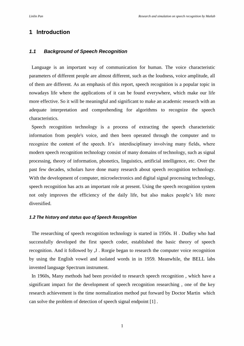
1 Introduction

1.1 Background of Speech Recognition

Language is an important way of communication for human. The voice characteristic

parameters of different people are almost different, such as the loudness, voice amplitude, all

of them are different. As an emphasis of this report, speech recognition is a popular topic in

nowadays life where the applications of it can be found everywhere, which make our life

more effective. So it will be meaningful and significant to make an academic research with an

adequate interpretation and comprehending for algorithms to recognize the speech

characteristics.

Speech recognition technology is a process of extracting the speech characteristic

information from people's voice, and then been operated through the computer and to

recognize the content of the speech. It’s interdisciplinary involving many fields, where

modern speech recognition technology consist of many domains of technology, such as signal

processing, theory of information, phonetics, linguistics, artificial intelligence, etc. Over the

past few decades, scholars have done many research about speech recognition technology.

With the development of computer, microelectronics and digital signal processing technology,

speech recognition has acts an important role at present. Using the speech recognition system

not only improves the efficiency of the daily life, but also makes people’s life more

diversified.

1.2 The history and status quo of Speech Recognition

The researching of speech recognition technology is started in 1950s. H . Dudley who had

successfully developed the first speech coder, established the basic theory of speech

recognition. And it followed by ,J . Rorgie began to research the computer voice recognition

by using the English vowel and isolated words in in 1959. Meanwhile, the BELL labs

invented language Spectrum instrument.

In 1960s, Many methods had been provided to research speech recognition , which have a

significant impact for the development of speech recognition researching , one of the key

research achievement is the time normalization method put forward by Doctor Martin which

can solve the problem of detection of speech signal endpoint [1] .


2

And in 1965, Doctor Tukey invented a famous algorithm, FFT (Fast Fourier Transform)

algorithm that can research the signal in the frequency domain, then In 1968, The most

important speech recognition technology, dynamic programming technology and linear

prediction analysis technology have been invented. [2]

There are many models didn’t adopted in the article, which are also significant for speech

recognition including: Hidden Markov Model (HMM), published by Doctor Baum in 70s that

the speech sequence can been constructed based on Markov chain. The HMM method can

well describe the time-varying and stationarity of speech signals, which can achieves a higher

modeling precision and become the starting of continuous speech recognition research.

In the mean time, vector quantization (VQ) theory was invented, and linear prediction

technology was developed more and more perfect. In 1980s, the artificial neural network

(ANN) technology has been applied in the field of speech recognition successfully. The

application of artificial neural network technology becomes a new way of researching voice

recognition, which has the advantage of non-linearity, robustness, fault tolerance and learning

characteristics. At the same time, the conjunctions speech recognition algorithms have been

proposed, which makes the speech recognition research start from micro to macro. [3]

In this period, the most famous researching achievement is the continuous speech

recognition system SPHINX, proposed by scholar Lee from Carnegie Mellon university of the

United States in 1988. In the decade of the 21st century, the experts have researched many

new methods of speech recognition in order to use it in the embedded devices. Although,

there are also many problems in the real applications, but the Speech recognition technology

is developing faster and faster. Recently, in the field of speech recognition, the direction of

researching has focused on the spoken dialogue system and the embedded speech

recognition system. Meantime, there are many projects of speech recognition, such as voice

recognition, robust speech recognition, speaker adaptation technology, large vocabulary

words recognition, speech recognition reliability evaluation algorithm and so on. The speaker

adaptation technology has achieved a big improvement in the fields of voice channel

normalization technology, maximum likelihood linear regression algorithm, bayesian adaptive

value algorithm etc.

Speech recognition technology based on HMM is now developed mature , more and more

people provided their own method based on it to get a better performance with various of

speech recognition algorithms. In this field, Doctor Wang from Tsinghua University have put

forward inhomogeneous improved hidden markov model of speech recognition. [4] In doctor

Wang's theory , the traditional HMM model has some problems in the speech recognition


3

application , and give a long distribution based inhomogeneous hidden markov model (DDB-

HMM) . Professor Zhao have put forward a hidden markov model by using even frame,

which can improve the robust performance in a noise environment. [4] With decades

optimization and evolution, speech recognition has developed with a quite mature extent that

widely spread to various of application.

1.3 Thesis Outline

The main goal in this thesis is to use the chosen models for training and processing the

signal, and select appropriate algorithms to analyze the computed data thus to simulate the

speech recognition procedure with different variables based on the researched theory. And

there are generally 4 sections composite of the report including:

Introduction section that describe the general background, history and status quo of Speech

recognition technology.

Theories on models of speech recognition technology contains signal pre-processing , which

describes a procedure to process signal with endpoint detection, pre-emphasis, framing and

windowing; And then it’s characteristic parameter extraction technology, author mainly used

Mel Frequency Cepstral coefficient extraction and related speech recognition algorithm in the

experiment. For analyzed the extracted parameter, Gaussian Mixture Model was utilized.

Then it will be the section detailed describing the process of the experiment based on the

Matlab. And the testing samples are taken by 3 pairs of words and numbers with different

variables to assume environmental difference, quantity of samples and syllable of words.

Those speech samples were then written into MATLAB program with MFCC characteristic

parameter extraction and GMM training model.

At last, it will be the discussion of the simulation result, and final conclusions about our

algorithm will be conducted. The experiment of this algorithm shows that the method in this

paper has relatively good performance. Simultaneously, author discussed the disadvantage of

the algorithm and some recommendation were also proposed aiming at deficiency in the

experiment.


4

1.4 Limitation in experiment

Several issues still exist in the practical application although GMM model has many

advantages,

1) .The problem of selection of GMM order

The system recognition rate will be low if the GMM order is too small, and it also generates

variety of problems such as increase the system computational complexity and the recognition

time if the order is too large. When the order is bigger than a certain special value, its

contribution to the performance of the system basic is negligible. In this case, it is very hard

to select a suitable order. An appropriate GMM order should be selected to balance the

performance and order, but it still may cause the experimental error of the accuracy.

2) .The length of training data

In most time, it is very difficult to obtain enough training data while the training data is

insufficient, the components of covariance matrix will be small. Those small values may

generate great influence on the performance of the system.

3) . The question of orthogonalization of GMM

The covariance matrix of gaussian mixture model is usually a full rank matrix which lead the

calculation work complicated. In practical application, the author will use the diagonal matrix

instead of the original covariance matrix to simplified computational complexity. But in fact,

each dimension of Covariance matrix is correlation and conditionality. One solution of this

problem is transforming the vector into the covariance matrix linearly, which can not only

simplified the calculation, but also not ignored the characteristic vector of each dimension .


5

2 Theory

The process of speech signal can be divided into the following several stages: firstly, the

language information produced in human's brain. Secondly, The human brain convert it into

language coding. And then express the language coding with different volume, pitch, timbre

and cycle. Once the last information coding completed, other people will hear the sound

generated by the speakers. Listeners could receive speaker's speech information, and extract

the parameter of speech and analysis the spectrum. And converting the spectrum signal into

excitation signal of auditory nerve by Neural sensor, then transform the signal to the brain

center by auditory nerve. At last, it’s been converted into language coding. This is main

process of speech generating and speech recognition in the physical phase. In this section,

theories will be surrounded with how signal can be simulated and recognized in scientific

method, they will explain the characteristics of speech signals, various pre-processing steps

involved in feature extraction, how characteristics of speech were extracted and how to

understand those characteristics when they are transformed to mathematical coefficient.

2.1 Signal sampling

A speech signal mainly contains two characteristics:

First, signal changes with the time where demonstrates short-time characteristics, which

indicates that signal is stable in a very short period of time. Second, spectrum energy of the

human’s speech signal normally centralized in frequency between 0-4000Hz. [5]

It is an analog signal when speak out from human, and it will convert to a digital signal

when input into computer, the conversion of this process introduce the most basic theory for

signal processing- signal sampling. It provides principles that the time domain speech analog

signal X(t) convert into the frequency domain discrete time signal X(n) while keeps

characteristics of the original signal in the same time. [5]And to fulfill discretization of the

sampling, another theory Nyquist theory is adopted. The theory requires sampling frequency

Fs must equal and larger than two times of the highest frequency for sampling and rebuilding

the signal, which can be represented as F≥2*Fmax , it offers a way to extract the enough

characteristics of the original analog signal in the condition of the least sampling frequency.in

the process of signal sampling. Due to inappropriate high sampling frequency lead to

sampling too much data （N=T/△t）with a certain length of signal (T), it will increase

unnecessary workload of computer and taken too much storage; On the contrary, the discrete


6

time signal won’t represent the characteristics of the original siganl if the sampling

frequency is too low and the sampling point are insufficient. [5]

So we always utilize about 8000Hz as the sampling frequency according to Nyquist Theory

that F≥2*Fmax

2.2 Signal Pre-processing

Voice signal samples into the recognizer to recognize the speech directly, because of the

non-stationary of the speech signal and high redundancy of the samples, thus it is very

important to pre-process the speech signal for eliminating redundant information and

extracting useful information. The speech signal pre-process step can improve the

performance of speech recognition and enhance recognition robustness .

Endpoint

checkpre-emphasis framing windows

Figure １pre-processing structure [6] [7]

It shows that the pre-processing module includes the module of endpoint checking, pre-

emphasis, framing, adding window. Endpoint checking can find the head and tail of useful

signal, pre-emphasis can reduce the signal dynamic range, framing can divide the speech data

into small chunks, Adding window can improve the frequency spectrum of the signal. [5]

2.2.1 Endpoint Detection

End point detection is one of a very significant technology in speech recognition and authors

used it as speech signal pre-treatment in the experiment. It can be defined as a technology to

detect the start and end point of the target signal so that the testing signal will be more

efficiently utilized for training and analyzing with a rather precise recognition result. [8] An

ideal end point detection contains the characteristics in reliability, accuracy, adaptability,

simplification, real-time processing and no need for noise pre-testing. [6] Generally, it

contains two methods in end point detection, one is based on entropy-spectral properties and

another is according to double threshold method. The one based on spectral entropy means

each frame signal is mainly divided into 16 sub-bands, and the selection will be those sub-

bands where distributed in between 250-4000Hz and energy does not exceed 90% of the total

in the frequency spectrum, then it will be the calculation of the energy after speech


7

enhancement and the signal-to-noise ratio of each sub-band. The evidence of the end-point

detection will be based on weighted calculation of whole spectral entropy with different SNR

adjustment. This method is effective for improving the detection rate in low SNR noisy

environment. And the second one, also called double threshold comparison method, it’s

normally used for single words detection by comparing the short-time average magnitude of

signal to short-time average threshold rate. The method is observed by the shape of average

magnitude, comprehensively judged by short-time average magnitude which is been settled as

a higher threshold T1 and lower threshold T2, in the mean while a lower threshold T3 for

short-time average threshold rate [6]

In practical experiment, end point detection will be a compiled program that system will

accurately test the start and end point so that to collect the valid data for decreasing

processing time and data for later use. After endpoint detection, the speech signal still

contains a large number of redundant information, which need us to extract the useful

characteristic parameters and remove the useless information. The model parameters, noise

model parameters and the adaptive filter parameter are calculated by the corresponding signal

segment. [8] Generally speaking, author will check the endpoint of speech voice by average

energy or the product of average amplitude value and zero crossing rate with the following

equation . [6]

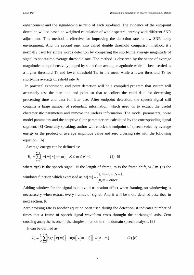
Average energy can be defined as:

1

2

0

,0 1N

n

m

E w m x n m m N

(1) [6]

where x(n) is the speech signal, N the length of frame, m is the frame shift, w ( m ) is the

windows function which expressed as 1, 0 ~ 1

0,

m Nw m

m other

Adding window for the signal is to avoid truncation effect when framing, so windowing is

necessacery when extract every frames of signal. And it will be more detailed described in

next section. [6]

Zero crossing rate is another equation been used during the detection, it indicates number of

times that a frame of speech signal waveform cross throught the horizongtal axis. Zero

crossing analysiss is one of the simplest method in time domain speech analysis. [9]

It can be defined as:

1

0

1sgn sgn 1

2

N

n

m

Z x m x m w n m

(2) [8]


8

The function here is to count the times that sign of signal x changes in the domain of 0 to N-1.

Here sgn[ ] is the sign function, which defined as sgn[𝑥] = {1, 𝑥 ≥ 0

−1，x ≤ 0 .Because of energy

of the devoiced sound is more concentrated in the high frequency section which makes its

zero crossing rate higher than the voiced sound, thus we can use zero crossing rate to

distinguish voiced and devoiced sound. [6]

Author made an example of double threshold shown in figure2 :

It manifests that the Double threshold detecting

endpoints of speech signal, the first figure is the

original signal and the second figure is the Zero

crossing rate while the third figure is the Energy.

And in the following technique can detect a speech

voice or not, if Zn > ratio(ration is a pre setting

Zero crossing rate) , then it’s a speech signal ,

namely , it’s been found the speech head . vice

versa, if Zn < ratio, then the speech signal is over,

which means speech tail will be found. The signal between head and tail is the useful signal

and thus the threshold in a big noise environment is adjustable. [8] [9]

2.2.2 Pre emphasis

The speech generated from the mouth will loss the information at high frequency, thus it

need the pre emphasis process in order to compensate the high frequency loss. Each frame

need to be emphasized by a high frequency filter. And for speech signal spectrum, the higher

the frequency is, the more serious the loss will be , where requires us do some operation for

the high frequency information, namely the pre emphasis. In the speech signal model, the pre

emphasis is a 1st order high pass filter. The speech will only remain the track section, it will

be very simple to analysis the speech parameter. [10]

The transform function of pre emphasis can be defined as:

1( ) 1H z z (3) [10]

According to the pre-emphasis function 1( ) 1H z z we got from the literatures, it can then

input the speech signal S(n) into the pre-emphasis module, thus we can got the signal and

transform it:

( )S z S z H z

0 0.2 0.4 0.6 0.8 1 1.2 1.4 1.6 1.8 2-1

0

1

Origin

al sig

nal

times

0 0.2 0.4 0.6 0.8 1 1.2 1.4 1.6 1.8 20

100

200

ZC

R

times

0 0.2 0.4 0.6 0.8 1 1.2 1.4 1.6 1.8 20

10

20

30

Energ

y

times

Figure ２Double threshold detecting endpoints of speech signal, [11]


9

11S z z

1S z S z

Parameter α is usually between 0 .94 and 0 .97 . [10]

Therefore, signal in time domain after pre emphasis can be defined as:

( ) ( ) ( 1)S n S n S n (4)

Based on the theory, the author can make the speech signal spectrum more flat and reduce the

signal dynamic range . Figure3 shows the simulation of pre emphasis.

Figure ３The pre emphasis of the original signal in time domain, [11]

And then do the FFT transform of Pre-emphasis speech signal as Figure 4 shows that after

Pre-emphasis, the high frequency part of the speech signal is enhanced obviously. Which

manifest the meaning of pre-emphasis process to enhance the high frequency section of

speech signal so that compensate the loss of high frequency for lip eradiation and inherent

decline of speech spectrum, and also eliminate impact of the lip eradiation. [12]

Figure ４The pre-emphasis of the original signal in frequency domain, [11]

2.2.3 Frame Blocking

The speech voice belongs to time-varying signal, which means the speech signal is a no-

linear signal with time changes. So we can’t use the linear time invariant analysis method to

observe the speech signal. In this case, the author cut the original signal into several small

0 0.2 0.4 0.6 0.8 1 1.2 1.4 1.6 1.8 2-1

-0.5

0

0.5

1

Origin

al

times

0 0.2 0.4 0.6 0.8 1 1.2 1.4 1.6 1.8 2-1

0

1

2

Pre

em

phasis

times

-1.5 -1 -0.5 0 0.5 1 1.5

x 104

0

100

200

300

400

500

600

700

frequency

mag

nitu

de

Original

-1.5 -1 -0.5 0 0.5 1 1.5

x 104

0

20

40

60

80

100

frequency

mag

nitu

de

Pre emphasis


10

pieces of continuous signal, because the speech signal has the characteristic parameters of

short time smooth. Typically, a frame of 20 - 30 ms could be considered for the short time

Time-Invariant property of speech signal. Framing can be classified as non-overlapping and

overlapping frames. Based on the characteristics of short-time smooth, the voice signal is in

the range of 20 - 30 ms is stable , which means the voice signal is stable in short time range,

[13] hence linear time invariant method can be used to analysis the speech signal then.

It is commonly believed that it should be contained 1 ~ 7 pitch in a speech frame. But in

most time, the pitch cycle of human is always different and changing . The pitch cycle of girl

is nearly 2ms, an old man is nearly 14ms. So it is very hard to select a sure value of N. The

range of N is always 100 ~ 200. if the sample frequency of speech is 10Khz, then the length

of each frame is about 10 ~ 20ms .

2.2.4 Adding Windows

The window function is a sequence with finite length, which used to select a desired frame

of the original signal and this process is a called windowing. Adding windows is a

continuation of short time speech signal processing, which means the speech signal multiplied

by a window function in time domain, simultaneously, it intercepted the signal part frequency

components. [14] And author made simple comparison with three types of window function

that most common to see as below including:

1) .Rectangular window:

1,0 1

0, 1

n Nw n

n N

(7) [14]

Rectangular windows function is a very simple window, which is replacing N values by

zeros, and the waveform will be suddenly turned on and off

2) .Hanning window:

2

0.5 0.5 cos ,0 11

0, 1

nn N

w n N

n N

(8) [14]

3) .Hamming window:

2

0.54 0.46 cos ,0 11

0, 1

nn N

w n N

n N

(9) [14]


11

The selection of different windows will determine the nature of the speech signal short-time

average energy. The shape of the window is different, but all of them are symmetric . And the

length of window will play a very important role in the filter. If the length of window is too

long, the pass band of filter will be narrow. Otherwise, if the length of window is too small ,

the pass band of filter will be wide, and the signal can be represented sufficiently equally

distributed. [12] [14]

Author made the example of three windows in time and frequency domain respectively below:

Figure ５Rectangular window, [11]

Figure ６Hanning window, [11]

Figure ７Hamming window, [11]

It’s can been observed from the figures above that all three windows have common

characteristics of low pass. The main lobe of Rectangular window is the smallest, while the

highest side lobe level and frequency spectrum leakage phenomenon is obvious. The main

lobe of hamming window is the widest, and it has the lowest side lobe level. The choice of the

window is critical for analysis of speech signal, utilizing rectangular window is easily loss the

details of the waveform, on the contrary, hamming window is more effective to decrease

frequency spectrum leakage with the smoother low pass effect. Therefore, Rectangular

window is more fit for processing signals in time domain and hamming window is more used

0 50 100 1500

0.2

0.4

0.6

0.8

1

n

x

Rectangular time domain(db)

0 0.2 0.4 0.6 0.8 1-100

-80

-60

-40

-20

0

w/pi

dB

Rectangular time frequency(db)

0 50 100 1500

0.2

0.4

0.6

0.8

1

n

x

Hanning time domain(db)

0 0.2 0.4 0.6 0.8 1-100

-80

-60

-40

-20

0

w/pi

dB

Hanning time frequency(db)

0 50 100 1500

0.2

0.4

0.6

0.8

1

n

x

hamming time domain(db)

0 0.2 0.4 0.6 0.8 1-100

-80

-60

-40

-20

0

w/pi

dB

hamming time frequency(db)


12

in frequency domain. [6] In the other hand, hamming window have relatively stable spectrum

for speech signal, and it helps to enhance the characteristics of the central section of signal,

which remains the better characteristics of original signal. [12] Besides, there’s another

purpose to use Hamming window for Gibbs phenomenon that relate to FFT that need to be

used later in calculating MFCC section, it’s a problem which caused by the truncation of

Fourier series or DFT of data with finite length with discontinuities at end points. It means

after FFT to the discrete periodic functions eg. rectangular pulses, and weight the data points.

The more points are taken, the peak of the waveform will be closer to the discrete points of

the original signals. When number of points are big enough, the value of the peak will be

approximate to a constant. Utilizing windows Hamming windows therefore is the good way to

force the end points to approximate to zero thus to ease the ripples of the Gibbs phenomenon.

[15]

So author prefer hamming window to process the signal in the experiment by the code

"hamming" function in Matlab.

w = hamming ( L ) ;

It returns an L point symmetric Hamming window in the column vector w. L should be a

positive integer. The coefficients of a Hamming window are computed from the following

equation .If the signal in a frame is denoted by s(n), n = 0,…N-1, then the signal will be

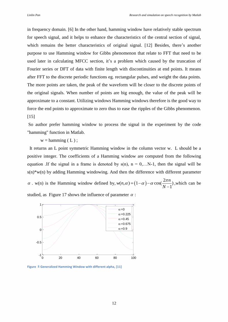
s(n)*w(n) by adding Hamming windowing. And then the difference with different parameter

. w(n) is the Hamming window defined by, 2

( , ) 1 cos( )1

nw n

N

,which can be

studied, as Figure 17 shows the influence of parameter :

Figure ８Generalized Hamming Window with different alpha, [11]

0 20 40 60 80 100-1

-0.5

0

0.5

1

=0

=0.225

=0.45

=0.675

=0.9


13

It shows a better observation when is between 0.45 to 0.675 and in the experiment I set the

value of 0.46 and use the hamming window as the filter, The simulation results is shown

in figure 18

Figure ９the result of Adding window, [11]

It can be observed that the signal will become smoother after the hamming window. As we

know, In signal processing theory, The window function is a mathematical function that is

zero-valued outside of some chosen interval. And as the results of pre process shown in the

theory explanation, the speech signal will become smoother and low dynamic range, which

manifest here we have get a relatively ideal signal to be processed. In summary, the hamming

windows are weighting functions applied to data to reduce the spectrum leakage associated

with finite observation intervals. It’s better to use the window to truncate the long signal

sequence into the short time sequence. In this way, the using of window in the pre-processing

phase will not only reduce the leakage of the frequency component, but also make spectrum

smoother.

2.3 The characteristic parameters of speech signal

Before the recognition of speech, characteristic parameters of the input speech signal is need

to be extracted. The purpose of characteristic parameters extraction is to analyze speech signal

processing and removes the redundant information which has nothing to do with speech

recognition and obtain the important information .Generally speaking, there are two kinds of

characteristic parameters, the first one is the characteristic parameters in time domain and the

second is in transform domain. The advantage of characteristic parameters in time domain is

simple calculation. However, it cannot be compressed and also not suitable for the

characterization of amplitude spectrum characteristics. [16]

0 0.005 0.01 0.015 0.02 0.025-0.4

-0.2

0

0.2

0.4

seconds

am

plit

ude

-1.5 -1 -0.5 0 0.5 1 1.5

x 104

0

2

4

6

8

frequency

magnitude

0 0.005 0.01 0.015 0.02 0.025-0.2

0

0.2

0.4

0.6

seconds

am

plit

ude

-1.5 -1 -0.5 0 0.5 1 1.5

x 104

0

2

4

6

frequency

magnitude


14

So far, the speech signal characteristic parameters are almost based on short-time spectrum

estimation, the author learnt 2 related parameters that can be used in Matlab including Linear

Predictive Coefficient, and the Mel frequency Cepstrum Coefficient in this research. The

method of Linear predictive analysis is one of the most important and widely used speech

analysis techniques. The importance of this method is grounded both in its ability to provide

accurate estimates of the speech parameters and in its relative speed of computation. The

method of Linear predictive analysis is based on the assumption that the speech can be

characterized by a predictor model, which looks at past values of the output alone; hence it is

an all pole model in the Z transform domain.

The method of Mel Frequency Cepstral Coefficients is also a powerful technique, which is

calculated based on the mel scale. Before calculating the MFCC coefficient, it is necessary

framing the whole speech signal into multi sub frames, the Hamming windows and Fast

Fourier transformation are computed for each frame. The power spectrum is segmented into a

number of critical bands by means of a filter-bank typically consists of overlapping triangular

filters which will adapt the frequency resolution to the properties of the human ear . The

discrete cosine transformation applied to the logarithm of the filter-bank outputs results in the

raw MFCC vector triangular filters. So the MFCC imitate the ear perception behavior and

give, good identification than LPC. [17]

2.3.1 MFCC

Mel Frequency Cepstral Coefficient proposed by Dr Davis, is the characteristic parameter

which widely used in speech recognition or speaker recognition. Before the Mel Frequency

Cepstral Coefficients, the researchers always use the Linear Prediction Coefficients or Linear

Prediction Cepstral Coefficients as the Characteristic parameters of speech signal. Mel

Frequency Cepstral Coefficients is the representation of short time power spectrum of a

speech signal, and it is calculated by DCT 1to convert into time domain, based on a linear

cosine transform of a log power spectrum on a nonlinear mel scale of frequency. Then the

result will be set of the acoustic vectors. [7]

MFCC are commonly used as Characteristic parameters in speech recognition algorithm. In

the theory of MFCC, the Critical Band is a very important concept which can solve problem

of frequency division, it is also an important indicator of Mel frequency. The purpose of

1 DCT: Abbreviated from discrete cosine transform, defined as a finite sequence of data points which establish a sum of cosine functions with different frequencies. [7]


15

introducing critical bandwidth is to describe the masking effect. When two similar or same

pitches voiced in the same time, human ear can’t distinguish the difference and only can

receive one pitch. The condition that two pitches can be received is that the weight difference

of two frequencies suppose two larger than certain bandwidth, and we called this as critical

bandwidth. [14] In critical bandwidth, if the sound pressure of a speech signal with noise is

constant, the loudness of speech signal with noise is constant then. But once the noise

bandwidth beyond the critical bandwidth, the loudness will change obviously. And its

expression defined as follows,

0.692

25 75 1.41000

cc

fBW

2 (32) [14]

The characteristics of the ear receiving process is thus been simulated by establishing the

critical bandwidth filter bank to achieving the recognition. The critical bandwidth filter bank

is a set of filters where center frequency of every filters in mel frequency domain are

distributed in linear and their bandwidth are always in the critical bandwidth range. [14] In

practical use, critical bandwidth will change with the changing of frequency, and is

proportional to the frequency growth. When the frequency is under 1000Hz, the Critical Band

is almost linear, approximately 100Hz, when the frequency is more then 1000Hz , the Critical

Band will growth exponently . Then it can divide the speech frequency into a series of

triangular filter series. [18] [19]

The Mel scale relates perceived frequency or pitch of a pure tone to its actual measured

frequency. Humans are much better at discerning small changes in pitch at low frequencies

than they are at high frequencies. Incorporating this scale makes our Characteristic parameters

match more closely what humans hear.

The formula for converting from normal frequency to Mel scale can be defined as:

( ) 1125 ln 1700

fM f

(33) [14]

Then we can get M-1(m) , the inverse function of above

/11251 700 1m

M m e (34) [14]

Then for implement and calculate MFCC:

Step1: Adding the hamming window to the input speech frame:

2 fc represent mel frequency.


16

( ) ( ) ( ),0 1l lx n x n w n n N (35) [6]

where

2

( ) 0.54 0.46cos ,0 11

nw n n N

N

(36) [14]

Step2: Do the calculation of FFT to get the signal in frequency domain.

Based on the equation 34, we can get the output of every filter thus to perform Si(k), the

Discrete Fourier Transform of the frames of the signal in short time,

2 /

1

( ) ( ) ( ) ,1N

j kn N

i i

n

S k s n h n e k K

(37) [14]

Where h(n) is an N sample long analysis window , K is the length of the DFT . The period

gram based power spectral estimate for the speech frame Si(k) is given by function:

21

( ) ( )i iP k S kN

(38) [14]

This is called the Periodogram estimation of the power spectrum, it helps to take the absolute

value of the complex fourier transform , and square the result .

The fast Fourier transform (FFT) is an algorithm which can calculate the discrete Fourier

transform more quickly than the DCT itself. The signal can be transformed from the time

domain to frequency domain, and vice versa. The most important advantage of the fast

Fourier transform is its calculation speed. Nowadays, the FFT is widely used in many

applications, such as signal process, science, communication and so on. The fast Fourier

transform were first proposed by Cooley and Tukey in 1965. And then, doctor Danielson-

Lanczos lemma have proposed the discrete Fourier transform, which can compute the fft by

discrete time domain. Normally, the length of data will be calculated by FFT is always a

power of two, when the length is not the power of two, we can add the points of zeros value

until the length is power of two. An efficient real Fourier transform algorithm or a fast

Hartley transform gives a further increase in speed by approximately a factor of two. [5]

The Fast Fourier transform algorithms can be divided into two classes, the first is

decimation in time, the second is decimation in frequency. The famous algorithm of Cooley

Tukey FFT, which first rearranges the input elements in bit-reversed order , then builds the

output transform . [5]

1 / 2 1 / 2 12 2 / 2 2 1 /2 /

2 2 1

0 0 0

N N Ni n k N i n k Nink N

n n n

n n n

a e a e a e

/ 2 1 / 2 12 / / 2 2 / / 22 /

0 0n n

N Nink N ink Neven ik N odd

n n

a e e a e

(39) [5]


17

Step3: Filter bank

To implement this filter bank, the window of speech data is transformed by using a Fourier

transform and taking the magnitude. The magnitude coefficients are then binned by

correlating them with each triangular filter. Here binning means that each FFT magnitude

coefficient is multiplied by the corresponding filter gain and the results accumulated. Thus,

each bin holds a weighted sum representing the spectral magnitude in that filter bank channel.

Fig. 10 illustrates the general form of this filter bank:

Figure １０filter bank starts at 0Hz and ends at 8000Hz, [11]

This figure shows a set of triangular filters that are used to compute a weighted sum of filter

spectral components so that the output of process approximates to a Mel scale. Each filter‘s

magnitude frequency response is triangular in shape and equal to unity at the centre frequency

and decrease linearly to zero at centre frequency of two adjacent filters. Normally the

triangular filters are spread over the whole frequency range from zero up to the Nyquist

frequency. However, band-limiting is often useful to reject unwanted frequencies or avoid

allocating filters to frequency regions in which there is no useful signal energy. The main

function of triangular band pass filters is smoothing the magnitude spectrum into to obtain the

envelop of the spectrum which can indicate the pitch of a speech signal is usually not

presented in MFCC.

This is a set of 20-40 (26 is standard ) triangular filters that the author apply to the

periodogram power spectral estimate from step 2. Our filter bank comes in the form of 26

vectors of length 257). Each vector is mostly zeros, but is non-zero for a certain section of the

spectrum. To calculate filter bank energies it need to multiply each filter bank with the power

spectrum, then add up the coefficients. Once this is performed there will left with 26 numbers

that give us an indication of how much energy was in each filter bank. [5]For a detailed

explanation of how to calculate the filter banks see below.


18

The main step of Computing the Mel filter bank：

Step1: Selecting a lower (300 ~ 600 Hz ) and upper ( 6000 ~ 10000 Hz )frequency .

Step2: Converting the upper and lower frequencies to Mels .

Step3: Computing the filter bank, It is assumed that there are M filters, The output of triangle

filter Y can be defined as:

1

1

1 1

11 1

, 1,2,.....,i i

i i

F F

i ii k k

k F k Fi i i i

k F F kY X X i M

F F F F

(40)

[14]

Where M is the number of filter , Xk is the energy of k th frequency point , Yi is the output

of i th filter , Fi is the centre frequency of i th filter .

Now the author create our filter banks. The first filter bank will start at the first point, reach

its peak at the second point , then return to zero at the 3rd point . The second filter bank will

start at the 2nd point, reach its max at the 3rd , then be zero at the 4th etc . A formula for

calculating these is as follows:

0, ( 1)

( 1), ( 1) ( )

( ) ( 1)( )

( 1), ( ) ( 1)

( 1) ( )

0, ( 1)

k f m

k f mf m k f m

f m f mH k

f m kf m k f m

f m f m

k f m

(41) [14]

where M is the number of filters the author want , and f is the list of M+2 Mel-spaced

frequencies . The centre frequency f(m) can be calculated by:

( 1) ( ) ( )

( ) ( )1

h ll

s

Mel f Mel fNf m Mel Mel f i

F M

(42) [14]

where fl is lower frequency, fh is the higher frequency . Fs is the sample frequency, Mel(-1)

the inverse function of Mel .

Step4: Although MFCC alone can be used as the characteristic parameters for speech

recognition, but here we can add up the log calculation to improve the performance in the

process, and it can be simply programmed by the following code in Matlab to calculate the

log of filter bank energies. So take the log of each of all the energies from step 3 and then we

can get the MFCC after FFT translation.

Step5: DCT, the abbreviation of discrete cosine transform, which can express a finite

sequence of data as a sum of cosine function value at different frequencies. Discrete cosine


19

transform is a very important technology in the applications of multimedia fields, such as the

lossy compression of jpeg and audio. The reason why DCT transform is calculated based on

the cosine function rather than sine functions is because of when calculate both of them, cos(-

X) = cos(X) and sin(-X)=-sin(X), which indicates cosine function will save half of the storage

cause it’s one step less compared with the sine function, and cosine function is more flexible

to get the value when it’s in between 180-360°by taking the inversely value of 0-180°,

while sine function can’t. Thus cosine functions are much more efficient than the sine

functions in compression, and the cosines functions can express a particular choice of

boundary conditions in differential equations. In particular, a DCT is a Fourier-related

transform similar to the discrete Fourier transform (DFT), but using only real numbers. There

are eight standard DCT variants, of which four are common. The most common variant of

discrete cosine transform is the type-II DCT, which is often called simply "the DCT". [5]The

formula can be defined as:

1

0

1cos , 0,..., 1

2

N

k n

n

X x n k k NN

(43) [5]

where N is the triangular band pass filters numbers, is the number of mel scale cepstral

coefficients. This transform is exactly equivalent to a DFT of real inputs of even symmetry

where the even-indexed elements are zero.

Step6: In order to express the dynamic Characteristic parameters of speech signal , the author

always add the 1-order cepstrum to the speech signal:

2

2

( ) ( ),1l l k

k

c kc P

(44) [5]

2.4 Recognition

2.4.1 GMM (Gaussian Mixture Model)

GMM, the abbreviation of Gaussian Mixture Model, which can be seen as a probability

density function. The method of GMM is widely used in many fields, such as recognition,

prediction, clustering analysis. The parameters of GMM are estimated from the training data

by Expectation-Maximization (EM) algorithm or Maximum A Posteriori (MAP) estimation.

Compared with many other model and method, the Gaussian Mixture Model has many

advantages, hence it is widely used in the speech recognition field. As a fact, the GMM can be


20

seen as a CHMM with only one state, but yet it can not be simply regarded as a hidden

markov model (HMM) due to GMM completely avoid the segmentation of the system state.

When compared with the HMM model, the GMM mode will make the researching of speech

recognition more simply, but the performance has no lossy. And the gaussian mixture model

which is calculating the characteristic parameters space distribution by the weight sum of

multi gaussian density function when compared with the VQ method, from this point of view,

the GMM has more accuracy and superiority. [20] It is very hard to match the process of

human's pronunciation organs, but we can simulate a model which express the process of

sound, and it can be implemented by building a probability model for speech processing,

while gaussian mixture model is the very probability model which can qualified the condition

.

The definition of gaussian mixture model

The formula of M order gaussian mixture model can be defined as:

( ) ( )M

t i i t

i l

P x p x

(52) [14]

where xt is a D dimension Speech Characteristic parameters vector, ( )i tp x is the element of

gaussian mixture model, namely the probability density function of each model. i is the

weight coefficient of ( )i tp x . M is the order of gaussian mixture model, namely the number of

probability density function. the author can know that:

1

1M

i

i

(53) [14]

1

1

22

1( ) exp

22

T

t i t iii t D

i

x u x up x

(54) [14]

Thus the element ( )i tp x of gaussian mixture model can be described the mean value and

covariance. [21]

EM algorithm is the abbreviation of expectation maximization, which is an iterative

method. The EM algorithm can search the maximum likelihood estimation of parameters in

statistical models. The EM algorithm can be divided into two steps, the first step is the

expectation (E) step, which can generate a function for the expectation of the log-likelihood.

The second step is the maximization (M) step, which can compute the parameters and

maximize the expected log-likelihood searched on the step E. In many research fields, the


21

Expectation maximization is the most popular technique, which is used to calculate the

parameters of a parametric mixture model distribution. It is an iterative algorithm with Three

steps: Initialization, the expectation step and the maximization step . [22]

Each class j of M clusters, which is constituted by a parameter vector ( θ ), composed by the

mean ( j ) and by the covariance matrix ( jP ). On the initial time, the implementation can

generate randomly the initial values of mean ( j ) and of covariance matrix ( jP ). The EM

algorithm aims to approximate the parameter vector (θ) of the real distribution.

Expectation step is responsible to estimate the probability of each element belong to each

cluster |j kP C x . Each element is composed by an attribute vector ( kx ). With initial guesses

for the parameters of our mixture model, The probability of hidden state i can be defined as

[20]:

,

1

| ,|

|

i t t i i

t t M

tm m t

m

PP x i i Pb xP i i x

P xP b x

(55) [22]

Maximization step is responsible to estimate the parameters of the probability distribution

of each class for the next step. First is computed the mean ( j ) of class j obtained through

the mean of all points in function of the relevance degree of each point.

The calculation of i i i :

1

1

1 1

( )1

' ( | , )1

( )

T

t Tt

i t tT Mt

t

t i

r i

P i i xT

r iT

(56) [22]

1 1

1 1

( ) | ,

( ) | ,

T T

t t t t t

t ti T T

t t t

t t

r i x P i i x x

r i P i i x

(57) [22]

2

1

1

| ,

| ,

T

t t t i

t

Ti

t t

t

P i i x x

P i i x

(58) [22]

The advantage of GMM is that the sample points after projection is not get a certain tags,

but also get the probability of each class that is an important information. The calculation of


22

GMM in each steps is very large and the solving method of GMM is based on EM algorithm,

where it is likely to fall into local extremum, which is related with the initial value. [21] [22]


23

2.5 Tools in the experiment.

The major tool to achieve the simulation experiment and analysis in this report is to utilize

Matlab where I use the version 2010. MATLAB is a numerical computing environment and

fourth-generation programming language which is Developed by MathWorks. MATLAB

allows matrix manipulations, plotting of functions and data, implementation of algorithms

from elementary functions like sum , sine , cosine , and complex arithmetic, to more

sophisticated functions like matrix inverse, matrix eigenvalues, Bessel functions, and fast

Fourier transforms, creation of user interfaces , and interfacing with programs written in other

languages , including C , C++ , Java , and Fortran .

And another toolbox which called VOICEBOX is used for speech processing, it consists of

MATLAB routines that are maintained by and mostly written by Mike Brookes [23]

The speech processing toolbox contains many speech process function, in this project, the

author has used the following functions.

frq2mel .m : Convert Hertz to mel scale;

mel2frq .m : Convert mel scale to Hertz;

rfft .m : FFT of real data;

rdct .m : DCT of real data;

enframe .m : Divide a speech signal into frames;

Lpc .m : Convert between alternative LPC representation;

kmeans .m : Vector quantisation, k-means algorithm;

melbankm .m : Mel filterbank transformation matrix;

melcepst .m : Mel cepstrum frontend for recogniser;

gaussmix .m : Fit a gaussian mixture model to data values;


24

3 Process and results

3.1 Process

3.1.1 Flow chart of the experiment

From the literature review, Pre-processing, MFCC Characteristic parameters extraction,

GMM recognition is the most important module in this the whole structure of algorithm. it

can be learnt that the new module of the speech recognition can be sort out into sequence of

pre-processing-MFCC-GMM implementation which gives relatively higher accuracy on

diverse conditions and in presence of noise, as well as for a wide variety of speech words and

hence this paper will be focusing on this particular area .

The whole algorithm flow chart can be described in figure 11 with the sequence of the

theory author introduced,

Speech signal

Pre processing

Train samples Test samples

Feature extraction Feature extraction

GMM

Check

recognition

Figure １１main flow of algorithm, [11]

The flow of the experiment will start with the recorded reference signal simples, which will

be first pre-process by the characteristic parameters extraction and then go through GMM

recognition and realized as the sound reference library, and then it will be the testing signal


25

simples that implemented by the same algorithms and routines where the output will be

extracted to compare with the reference therefore to achieving the recognition.

3.1.2 Speech recognition system evaluation criterion

After the signal processing and simulated recognition, the result requires a criteria to

represent and analysis. Normally for the isolated word recognition system, whole word

recognition rate to evaluate and identify accuracy will be defined as:

right

total

NR

N

(58)

where R is recognition rate, rightN is the number of right recognition words, totalN is the total

number of words .

For the continuous speech recognition system, sentence recognition rate can be achieved by

assessing the system recognition accuracy where quantity of the sentence recognition rate is

often affected by the number of sentence and the influence of language model information

utilization .

right word

word

total word

NR

N

(59)

wordR is the identification accuracy, right wordN is the number of right recognition words ,

total wordN is the total number of words .

In this project, the first method will be used in the analysis due to the focus in this project is

the recognition of isolated word recognition system and some simple words as samples like

“Yes and No”, ”on and off” will be utilized.


26

3.2 Result

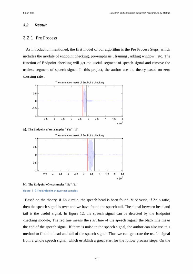
3.2.1 Pre Process

As introduction mentioned, the first model of our algorithm is the Pre Process Steps, which

includes the module of endpoint checking, pre-emphasis , framing , adding window , etc. The

function of Endpoint checking will get the useful segment of speech signal and remove the

useless segment of speech signal. In this project, the author use the theory based on zero

crossing rate .

a). The Endpoint of test samples "Yes" [11]

b). The Endpoint of test samples "No" [11]

Figure １２The Endpoint of two test samples

Based on the theory, if Zn > ratio, the speech head is been found. Vice versa, if Zn < ratio,

then the speech signal is over and we have found the speech tail. The signal between head and

tail is the useful signal. In figure 12, the speech signal can be detected by the Endpoint

checking module, The red line means the start line of the speech signal, the black line mean

the end of the speech signal. If there is noise in the speech signal, the author can also use this

method to find the head and tail of the speech signal. Thus we can generate the useful signal

from a whole speech signal, which establish a great start for the follow process steps. On the

0.5 1 1.5 2 2.5 3 3.5 4 4.5 5

x 104

-1

-0.5

0

0.5

1

The simulation result of EndPoint checking

0.5 1 1.5 2 2.5 3 3.5 4 4.5 5 5.5

x 104

-1

-0.5

0

0.5

1

The simulation result of EndPoint checking


27

other hand, if the speech signal is a continuous sequence, the signal can be divided into the

continuous sequence in some isolated words.

Pre emphasis is widely used in the field of telecommunications, digital speech recording and

so on. In a high speed digital transmission, the process of Pre emphasis is always used to

improve signal quality at the output of the system. In the process of signal transmission that

the signal may be distorted so that the pre emphasis is used to distort the transmitted signal to

correct for this distortion. In a whole speech process system, the Pre emphasis is the first part

of noise reduction technique, higher frequencies are boosted before they are transmitted or

recorded onto a storage medium.

In this project, the parameter of pre-emphasis function is 0 .95, which make 95% of any

one sample is presumed to originate from previous sample. Pre emphasis can be expressed as

the following formula:

1( ) 1 0.95H z z

(1)

( ) ( ) 0.95 ( 1)s n s n s n

(2)

In MATLAB , the code author has written is:

yPreEmp = filter ([1 , -0 .95] , 1 , y);

Then by using filter function directly it comes a filtered data sequence using a digital filter

where works for both real and complex inputs. The filter is a direct form II transposed

implementation of the standard difference equation and this make Pre-emphasis a filter .

Figure １３The signal after pre emphasis [11]

Figure above shows that the original speech signal becomes more stable after Pre-emphasis ,

and this conduct reducing the dynamic range which makes the signal become suitable for

processing .

0 500 1000 1500 2000 2500-1

-0.5

0

0.5

1

1.5

2

2.5

original

Pre emphasis


28

Figure １４The signal after pre emphasis, [11]

And the spectrum shows that the system can compensate the high-frequency part which was

suppressed during the sound production process by pre emphasis. And then it’s been the

framing part to sampling the signal and framing operation can convert the whole frame into N

short frame from short frame 1 to N, and it followed by the main code as follows:

Frame

Sub-Frame1 ……Sub-Frame2

overlapped

Sub-FrameN-1 Sub-FrameN

overlapped

Figure １５framing, [13]

Length of each frame is recorded 256 samples points as 22.8ms. The overlap of frame is 12

samples. Then, the speech signal can be analysis by Linear time invariant method.

As the theory introduced, the purpose of utilizing hamming windows is to ease the ripples

of the Gibbs phenomenon, which are the result of the Fourier series approximation, a series of

continuous functions, over the discontinuous desired magnitude response.

3.2.2 MFCC

Now computation of MFCC will be discussed step by step. The main stage for calculating the

MFCC coefficients is taking the log spectrum of the windowed waveform which will then be

smoothened out by triangular filters and then compute the DCT of the waveform to generate

the MFCC coefficients. In programming, experiment procedure for this part was followed by

the following steps based on the literature reviews,

-1 -0.5 0 0.5 1

x 104

0

10

20

30

40

50

60

70

80

frequency

magnitude

-1 -0.5 0 0.5 1

x 104

0

5

10

15

20

25

30

35

40

frequency

magnitude


29

Speech signal Short time energy Pre emphasis

Adding windowsFFTT filter bank

Log calculation DCT MFCC

Figure １６the extraction step of MFCC [7]

It’s total 9 steps of MFCC extraction where the first four steps are the signal pre-process

including signal input, short time energy, pre emphasis, adding windows as we mentioned

before. And the following five steps are the extraction process , including the FFT , filter bank

,Log , DCT and MFCC .

FFT , the abbreviation of the Fast Fourier Transform, is essentially transformed from the

discrete-time signal from time domain into its frequency domain. Algorithm is the Radix-2

FFT Algorithm where we can directly use the MATLAB code

y=fft(x,n);

Here, the "FFT" function is used to get the frequency domain signal. The following

spectrum are respectively represent time domain and frequency domain, where the spectrum

in frequency domain only display the right section from 0. So the frequency domain spectrum

are always about half of the length compared with the time domain spectrum. The word of

“YES” is disyllable, which means the total range of it will be longer that other monosyllable

words.

a). The frequency signal of speech word "Yes" [11]

b). The frequency signal of speech word "No" [11]

0 500 1000 1500 2000 2500-0.8

-0.6

-0.4

-0.2

0

0.2

0.4

0.6time domain

0 200 400 600 800 1000 1200 14000

0.2

0.4

0.6

0.8

1frequency domain

0 1000 2000 3000 4000 5000-0.4

-0.3

-0.2

-0.1

0

0.1

0.2

0.3time domain

0 500 1000 1500 2000 25000

0.2

0.4

0.6

0.8

1frequency domain


30

Figure １７The frequency signal after fft

a). The frequency signal of speech word "on" [11]

b). The frequency signal of speech word "off"

Figure １８The frequency signal after FFT [11]

After doing DFT and FFT transform, The signal will be changed from the discrete time

signals x(n) to the frequency domain signal X(ω) . The spectrum of the X(ω) is the whole

integral or the summation of the all frequency components. When talking about the speech

signal frequency for different words, each word has its frequency bandwidth, For examples,

Speech "Yes" has the frequency range between 200 and 400, while speech "No" has the

frequency range between 50 and 300, and speech "On" has the frequency range between 100

and 200 , speech "off" has the frequency range between 50 and 200, all of them are not just a

single frequency. And the max value of frequency spectrum is 1, where is the result of

normalization after FFT. The normalization can reduce the error when comparing the

spectrums, which is good for the speech recognition. On the other hand, the result of FFT

transform is always a complex value, which is not suitable for other operation, so here adopt

absolute values of the FFT and lead it to be a real value like the figure 20 and 21 shown. The

frequency analysis shows that that different timbre in speech signals corresponds to the

different energy frequency distribution.

It’s the filter bank followed by the normalization of the signal, I multiple the magnitude

frequency response by a set of 20 band pass filters to get the log energy of each triangular

band pass filter. As we know, the filters used are triangular band pass filter. The positions of

0 1000 2000 3000 4000-1

-0.5

0

0.5

1

1.5time domain

0 500 1000 1500 20000

0.2

0.4

0.6

0.8

1frequency domain

0 1000 2000 3000 4000-0.4

-0.3

-0.2

-0.1

0

0.1

0.2

0.3

0.4time domain

0 500 1000 1500 20000

0.2

0.4

0.6

0.8

1frequency domain


31

these filters are equally spaced along the Mel frequency, which is related to the linear

frequency. They are equally spaced along the mel scale which is defined by

10( ) 2595 log 1700

fMel f

As theory mentioned, the goal of computing the discrete cosine transform (DCT) of log filter-

bank is to get the uncorrelated MFCC. In this project, With our MFCC computation, the DCT

is applied to the output of 40 mel scale filters. The following value of the output of the filters.

-2.586 , -2.627 , -2.086 , -2.100 , -2.319 , -1.975 , -2.178 , -2.195 , -1.953 , -2.231 ,

-2.021 , -1.933 , -1.966 , -1.514 , -1.646 , -1.530 , -1.488 , -2.062 , -2.286 , -2.348 ,

-2.538 , -2.696 , -2.764 , -2.852 , -2.950 , -2.843 , -2.454 , -2.438 , -2.655 , -2.318 ,

-2.457 , -3.171 , -3.413 , -2.628 , -2.558 , -3.296 , -3.576 , -3.560 , -3.462 , -3.396 ;

Figure １９The results of discrete cosine transform [11]

Figure 20 is the waveform of the output of 40 mel scale filters, all the value of mel scale

filters is negative. Since the author has calculated the FFT, DCT which can transform the

frequency domain into a time like domain. Obtained Characteristic parameters are similar to

cepstrum, thus it is referred to the mel scale cepstral coefficients, or MFCC. MFCC can be

used as the Characteristic parameters for speech recognition. Compared with the MFCC

coefficient before DCT, The data size is compressed obviously, so the function of the DCT

transform is a compression step. Typically with MFCCs, you will take the DCT and then keep

only the first few coefficients, which is the same theory of DCT used in JPEG compression.

So, When you take the DCT, you will discard the higher coefficients, and only keeping the

parts that are more important for representing a smooth shape. The higher-order coefficients

that you discard are more noise-like and are not important to train. To sum up, DCT transform

can remove the higher-order coefficients and enhance the training performance.

And then it flows to the main steps of generating a set of MFCC coefficient, these are

obtained from a band-based frequency representation, and then with a discrete cosine

0 5 10 15 20 25 30 35 40-4

-3.5

-3

-2.5

-2

-1.5

-1


32

transform. The DCT is an efficient approximation for principal components analysis, and it

allows a compression, or reduction of dimensionality, of the data, thus to reduce some band

readings to a smaller set of MFCCs. A small number of Characteristic parameters end up

describing the spectrum. The MFCCs are commonly used as timbral descriptors.

a). The MFCC of "Yes" b). The MFCC of "No"

c). The MFCC of "ON" d). The MFCC of "OFF"

Figure ２０MFCC 3-D view plot (MFCC are result in sets of parameters without any unit) [11]

The value of MFCC is given in MFCC result of Appendix B.

MFCC is a very robust parameter for modelling the speech as it can be modelled as MFCC

kind of models the human auditory system and hence makes the reduction of the frame of a

speech into the MFCC coefficients a very useful transformation as now we have an even more

accurate transform to deal with for the recognition of the speakers. The other thing is that

MFCC is the tool that produces very high level of accuracy when used as a parameter model

for modelling the speech and hence for my study I have given focus in this area.

3.2.3 GMM

A Gaussian mixture model is a probabilistic model that assumes all the data points are

generated from a mixture of a finite number of Gaussian distributions with unknown

parameters. One can think of mixture models as generalizing k-means clustering to

incorporate information about the covariance structure of the data as well as the center of the

latent Gaussians.

0

5

10

15

0

2

4

6

8-60

-40

-20

0

20

0

5

10

15

0

5

10

15-40

-20

0

20

40

0

5

10

15

0

5

10

15-60

-40

-20

0

20

0

5

10

15

0

5

10

15-40

-30

-20

-10

0

10

20


33

The main steps of GMM is "ESTIMATION STEP" and "MAXIMIZATION STEP".

Expectation Maximisation (EM) is a well established maximum likelihood algorithm for

fitting a mixture model to a set of training data. It should be noted that EM requires an a priori

selection of model order, simultaneously, the number of M components to be incorporated

into the model. Often a suitable number may be selected by a user, roughly corresponding to

the number of distinct colors appearing in an object to be modelled. The problem of fully

automating this process, known as Automatic Model Order Selection, has been addressed in.

Now, the author will introduce the most important step:

·ESTIMATION STEP which suppose to represent the model, but not the assignment of

individual points,

[ lBM , lB ] = func_multi_gauss( X , mu , sigm , c );

LLH = mean( lB );

lgam_m = lBM - repmat ( lB , [ 1, M ] );

gam_m = exp ( lgam_m );

·MAXIMIZATION STEP that we can learn the assignment of individual points, but not the

model.

sgam_m = sum ( gam_m ) ;

new_c = mean ( gam_m ) ' ;

............................

new_sigm = max (new_sigm , min_sigm ) ;

After simulation, the author will get the new parameter of Gaussian mixture model, The

Results of Expectation Maximisation (EM) is given in GMM result of Appendix B.


34

3.3 Simulation and Analysis

3.3.1 Algorithm flow chart

We have introduced the designing of the speech recognition in the methodology chapter that

the final module is the recognition module and the system will output the speech content

based on MFCC extraction and GMM training, where the logic of the main flows is shown

below according to all steps introduced in previous chapter:

Speech signal

Pre process

Pre emphasis

framing

Hamming window

FFT

Mel filter bank

LOG

DCT

GMM parameter

Iteration GMM

LLR calculation

Whether

convergence

GMM train result

TEST

Train Test

Figure ２１flow of algorithm [11]

Generally Speaking, The function of each steps is:

1 ) . Step " Speech signal ": Recording some samples of English words, " Yes "," No "," On

"," Off ", from different person in different environment, In this project, the author will record

the signal both in a very quiet environment and the noisy environment. And also recording the

digital number from " 0 " to " 9 " in a quiet environment.

2 ) . Step " Train & Test ": Dividing the samples into training set and testing set. Training set

is a standard sample, and the testing set is the samples from different person in different

environment. The author will train the GMM model based on the training sample set and test

the system based on the testing set.

3 ) . Step " Pre process ": Doing the pre process of pre emphasis, framing, adding windows. In

this step, the author will program the matlab code to realize the function.


35

4 ) . Step " FFT ": Converting the signal in time domain into linear spectrum, and calculating

the square of the absolute value. In this step, the system will calculate the result in the

frequency domain.

5 ) . Step " Mel filter bank ": Calculating the Mel spectrum by Mel filter bank. The MFCC

coefficient will be the Characteristic parameters of the system.

6 ) . Step " Log ": Calculating the Log of Mel spectrum.

1

2

0

( ) ln ( ) ,0N

m

k

S m X k H k m M

.

7 ) . Step " DCT ": Getting the MFCC parameter by calculating DCT after LOG,

1

0

( 1/ 2)( ) ( ) cos ,0

M

M

n mc n S m m M

M

8 ) . Step " GMM ": Setting the initial parameter randomly, and Starting iterative calculation,

until meet the convergence conditions. the convergence condition is:

if

1

1

log | log |100

log |

t t

t

L X L X

L X

then the result is meeting the convergence

conditions.

9) . Step " TEST ": Using different samples to test the performance.

The algorithm can make every gaussian distribution of the GMM model as one kind, The

parameter of Mean is the position in Characteristic parameters space of different sample

Characteristic parameters, which is the most important parameter in GMM, The variance is

the density of data distribution, the weight is the number of data.

3.3.2 Simulation result Analysis

In this chapter, author simulated the designed systems and the only task of operator is to run

the program and record speech signals. Two sets of train speech signal and ten set of test

speech signal recorded. In the first experiments, speech signals will record from the three

different people both in quiet environment and noisy environment, and author has also

recorded a standard as the training samples. The content of first speech is "YES" and "NO" is

the pair of word different syllable, and the second one is "ON" and "OFF" with the similar

pronunciation. In the testing, the author will play "YES" and "NO" or "ON" and "OFF" 10

times respectively, in both quiet environment and noisy environment. In the second

experiments, number 0~9 from one person have been recorded. The goal of this experiment is

checking the performance of the algorithm in a real application. Author tested the number 10


36

times. The statistical simulation results of environment 1 and environment 2 will be put in

tables and will also be plotted and been discussed in next chapter.

And the following result are 3 groups of simulation where tested in the quiet lab room in

Arhus University by 3 different people with the content of speech is " Yes " and " No " with

different pronunciation basis and each of the group have taken 10 times testing samples

respectively to ensure the validity and accuracy of the experiment;

The speech signal from People 1.

Figure ２２3mean errors for the train signals with test signals, people 1 [11]

Here the definitions of error is 1 2( ( ) ( ))Err abs mean MFCC mean MFCC , Table 1 shows

the result of this test:

Table 1indicates the results for train signals “Yes” and “No” as the information given at the test Results, people 1 [11]

times error Final output Times error Final output

1 0. 0018 Yes 11 2. 2490 No

2 0. 0032 Yes 12 2. 2508 No

3 0. 0028 Yes 13 2. 2483 No

4 0. 0081 Yes 14 2. 2461 No

5 0. 0017 Yes 15 2. 2496 No

6 0. 0043 Yes 16 2. 2250 No

7 0. 0003 Yes 17 2. 2508 No

8 0. 0082 Yes 18 2. 2532 No

9 0. 0002 Yes 19 2. 2510 No

10 0. 0009 Yes 20 2. 2496 No

3 Right figure means in total 20 times simulating result, the input for 1-10th times are recognized as “NO” cause the algorithm calculate that the value of redline “No” is bigger than the blueline “YES”. Similarly, 11-20th times are recognized as “YES”. And figure behind for other simulating result has same meaning to observe the recognition result precisely.

0 5 10 15 200

0.002

0.004

0.006

0.008

0.01

0.012

0.014

times

Mean e

rror

Yes

No

0 2 4 6 8 10 12 14 16 18 200

0.5

1

1.5

2

2.5

times

Mean e

rror

Yes

No


37

Total successful probability(Yes) 100% Total successful probability(NO) 100%

The speech signal from People 2

Figure ２３mean errors for the train signals with test signals, people 2 [11]

Table 2the results for train signals “Yes” and “No” as the information given at the test Results, people 2 [11]


1 0. 0011 Yes 11 1. 6819 No

2 0. 0036 Yes 12 1. 6833 No

3 0. 0038 Yes 13 1. 6834 No

4 0. 0062 Yes 14 1. 6794 No

5 0. 0054 Yes 15 1. 6812 No

6 0. 0065 Yes 16 1. 6853 No

7 0. 0043 Yes 17 1. 6849 No

8 0. 0026 Yes 18 1. 6856 No

9 0. 0100 Yes 19 1. 6836 No

10 0. 0047 Yes 20 1. 6846 No


The speech signal from People3.

Figure ２４mean errors for the train signals with test signals, people 3 [11]

0 2 4 6 8 10 12 14 16 18 200

0.005

0.01

0.015

0.02

times

Mean e

rror

Yes

No

0 2 4 6 8 10 12 14 16 18 200

0.5

1

1.5

2

times

Mean e

rror

Yes

No

0 2 4 6 8 10 12 14 16 18 200

0.002

0.004

0.006

0.008

0.01

0.012

0.014

times

Mean e

rror

Yes

No

0 2 4 6 8 10 12 14 16 18 200

0.2

0.4

0.6

0.8

1

1.2

1.4

times

Mean e

rror

Yes

No


38

Table 3mean errors for the train signals with test signals, people 3 [11]


1 0. 0006 Yes 11 1. 2252 No

2 0. 0005 Yes 12 1. 2249 No

3 0. 0101 Yes 13 1. 2219 No

4 0. 0002 Yes 14 1. 2197 No

5 0. 0091 Yes 15 1. 2257 No

6 0. 0104 Yes 16 1. 2224 No

7 0. 0000 Yes 17 1. 2225 No

8 0. 0032 Yes 18 1. 2279 No

9 0. 0042 Yes 19 1. 2261 No

10 0. 0042 Yes 20 1. 2240 No


We can observe from three groups of testing of the word “Yes” and “No” reveals the

excellent with all 3 testing has 100 successful probability to recognition.

And then, the simulation goes other round of test with 3 groups of testing in the quiet lab

room in Arhus University by 3 different people with the content of speech is " On " and "

Off " in same pronunciation, and each of the group have taken 10 times testing samples

respectively to ensure the validity and accuracy of the experiment;


Figure ２５, mean errors for the train signals with test signals , people 1 [11]

Table 4the results for train signals “On” and “Off” as the information given at the test Results, people 1 [11]


1 0. 0078 On 11 2. 1320 Off

0 2 4 6 8 10 12 14 16 18 200

0.005

0.01

0.015

0.02

0.025

times

Mean e

rror

ON

OFF

0 2 4 6 8 10 12 14 16 18 200

0.5

1

1.5

2

2.5

times

Mean e

rror

ON

OFF


39

2 0. 0037 On 12 2. 1362 Off

3 0. 0062 On 13 2. 1280 Off

4 0. 0042 On 14 2. 1392 Off

5 0. 0087 On 15 2. 1364 Off

6 0. 0115 On 16 2. 1286 Off

7 0. 0066 On 17 2. 1258 Off

8 0. 0082 On 18 2. 1296 Off

9 0. 0117 On 19 2. 1417 Off

10 0. 0049 On 20 2. 1340 Off

Total successful probability(On) 100% Total successful probability(Off) 100%


Figure ２６mean errors for the train signals with test signals,people 2 [11]

Table 5results for train signals “On” and “Off” as the information given at the test Results, people 2 [11]


1 0. 0239 On 11 2. 5630 Off

2 0. 0191 On 12 2. 5694 Off

3 0. 0261 On 13 2. 5639 Off

4 0. 0184 On 14 2. 5718 Off

5 0. 0153 On 15 2. 5680 Off

6 0. 0304 On 16 2. 5605 Off

7 0. 0218 On 17 2. 5621 Off

8 0. 0164 On 18 2. 5660 Off

9 0. 0209 On 19 2. 5742 Off

10 0. 0210 On 20 2. 5670 Off


The speech signal is from People3.

0 2 4 6 8 10 12 14 16 18 200.005

0.01

0.015

0.02

0.025

0.03

0.035

times

Mean e

rror

ON

OFF

0 2 4 6 8 10 12 14 16 18 200

0.5

1

1.5

2

2.5

3

times

Mean e

rror

ON

OFF


40

Figure ２７mean errors for the train signals with test signals, people 3 [11]

Table 6the results for train signals “On” and “Off” as the information given at the test Results, people 3 [11]


1 0. 0135 On 11 3. 1598 Off

2 0. 0062 On 12 3. 1660 Off

3 0. 0158 On 13 3. 1613 Off

4 0. 0104 On 14 3. 1733 Off

5 0. 0096 On 15 3. 1652 Off

6 0. 0158 On 16 3. 1592 Off

7 0. 0149 On 17 3. 1597 Off

8 0. 0049 On 18 3. 1633 Off

9 0. 0132 On 19 3. 1715 Off

10 0. 0103 On 20 3. 1670 Off


The results of speech “on” and “off” in the quiet environment with similar pronunciation

shows that the performance is perfect and the total successful probability is 100%. And the

experiment proceed in the next step to test how the simulation could be outcome when the

environment is more close to the reality with different level of the noise, and the test will take

same indicator, with speech of “on” and “off”, “Yes” and “No” and each of the groups will

sampling 10 times, where the only variable changed is that we will add the noise with

different SNR level,

First is the output of the content of speech is " On " and " Off " , the author have added the

noise before recognition module. So the reference signal here is the overlapped sound with

clear speech and noise in different SNR in 9,7,5,3 and 1dB to analysis the performance in the

test, operation module is as follows,

0 2 4 6 8 10 12 14 16 18 200

0.005

0.01

0.015

0.02

0.025

times

Mean e

rror

ON

OFF

0 2 4 6 8 10 12 14 16 18 200

0.5

1

1.5

2

2.5

3

3.5

times

Mean e

rror

ON

OFF


41

Figure ２８Add noise flow chart [5]

Table 7the results for train signals “On” and “Off” with different noise [11]

Times SNR=9 SNR=7 SNR=5 SNR=3 SNR=1

1 off off Off off On

2 off off Off off Off

3 off off Off on On






9 off off Off on On












Performance 100% 100% 100% 90% 25%

The table indicates that SNR level can be adjusted to 5 and the system can still recognize the

right testing word “off” with 100% accuracy, but when the SNR is lower than that level the

trained signal appears error with match the reference signal and the performance begins to

weaken, and the performance is really poor that only matches 25% recognition probability

when SNR level is 1. The poor result when SNR equal 1 also reveal the limitation for the

Overlapped sound

Clear speech

Noise Speech recognition Result


42

algorithms I choose, it can be assumed here that when the noise in the certain degree, in

between 1dB-3dB in our case, this conjected recognition won’t work well anymore.

And it followed by the testing of “Yes and No” that added the noise with different level of

SNR 9,7,5,3,1dB to analysis the performance as table 8 shown,

Table 8the results for train signals “Yes” and “No” with different noise [11]

Times SNR=9 SNR=7 SNR=5 SNR=3 SNR=1

1 no No No no No

2 no No No yes Yes

3 no No No no No

4 no Yes Yes yes Yes

5 no Yes Yes yes Yes

6 no No No no No

7 no No No no Yes

8 no No No no No

9 no No No no No

10 no No No no No

11 no No No yes Yes

12 no No No yes Yes

13 no No No no No

14 no No No yes No

15 no No No no No

16 no No No no No

17 no No No no No

18 no No No no No

19 no No No yes Yes

20 no No No no No

Performance 100% 90% 90% 65% 65%

It can be observed that noise impact is different compared with word ”Yes and No” and ”On

and off”. When testing the word “No”, it describes that the performance will be decrease after

taken SNR 7 or below, and become weak when SNR is less than 3. The recognition of the

word “Yes and No” is relatively stable and gradually drop off as the noise level is stronger,

while the word “On and off” performs good when SNR is 5 or larger but will dramatically

drop the accuracy when SNR level is lower than 3 from 90% to 25%. In summary, the current

simulation system is more appropriate to use the word “On and Off” which is the


43

monosyllable when the recognition environment is relatively quiet and the noise is small, and

part for recognizing the disyllable or more complex words need to be implemented more

technique to improve but it will be more easier to recognize when the paring words with

different syllable in more noisy environment.

In the experimental stage, I also utilize the simulation of the speech of simple numbers from

“0” to “9” to verify and ensure the feasibility and validity of the simulation system, and the

test of numbers is also in the environment of the quite lab room with my own pronunciation,

In this test, I will analysis the performance of the MFCC-GMM simulation system in multi

testing samples from zero to nine, and the result is shown in below,

Table 9 the results for train signals “0” “9” as the information given at the test Results [11]

times 1 2 3 4 5 6 7 8 9 10 Accuracy

0 0 0 0 0 0 0 9 9 9 9 60 %

Error 0.6635 0.6579 0.6191 0.5880 0.5811 0.5677 0.5231 0.5058 0.5560 0.5099

1 1 1 1 1 1 1 1 1 1 1 100 %

Error 0.2341 0.3043 0.4127 0.4511 0.4685 0.5410 0.5531 0.6403 0.6563 0.7202

2 2 2 2 2 2 2 2 2 2 2 100 %

Error 0.1629 0.1274 0.0484 0.0798 0.0761 0.0833 0.0595 0.0333 0.0052 0.0646

3 3 3 3 3 3 3 3 3 3 3 100 %

Error 0.5211 0.4148 0.4232 0.3781 0.2464 0.3113 0.2751 0.2560 0.2091 0.2141

4 4 4 4 4 4 4 4 4 4 4 100 %

Error 0.2255 0.1856 0.1123 0.1985 0.0305 0.2245 0.0359 0.0539 0.0314 0.0779

5 5 5 5 5 5 5 5 5 5 5 100 %

Error 0.9158 1.1218 1.2795 1.4027 1.5248 1.5946 1.5572 1.6183 1.8048 1.8291

6 6 6 6 6 6 6 6 6 6 6 100 %

Error 0.1160 0.0996 0.1020 0.0844 0.0855 0.0455 0.0423 0.0380 0.0451 0.0387

7 7 7 7 7 7 7 7 7 7 7 100 %

Error 0.1741 0.0965 0.0268 0.0221 0.0973 0.1474 0.0917 0.2241 0.1639 0.2217

8 8 8 8 8 8 8 8 8 8 6 90 %

Error 0.1469 0.1641 0.1207 0.0899 0.1294 0.0615 0.0900 0.0904 0.0606 0.0464

9 9 9 9 9 9 9 9 9 9 9 100 %

Error 0.5794 0.5088 0.4672 0.4262 0.3911 0.3739 0.3021 0.3847 0.3620 0.3117

Total successful probability 95%

The simulation result of numbers from “0” to “9” manifest the system is very stable and

recognized in the quiet environment with similar result of testing of “Yes and No” ,”On and


44

Off”, we can told that system can be perfectly used on very simple monosyllable that they can

almost achieve with the 100% accuracy, but when the word becomes complex to pronounce ,

for example the word “zero” and word “ eight” which the system recognized with the output

“nine” and “six” in some times, the simulation system will have problem to recognizing and

accuracy will drop off even in the ideal environment. And another variable as this chapter

mentioned earlier that the noise level will have very significant impact with the recognition

accuracy, and the best scenario for use the system is that the SNR level of signal should be

higher that 5 at least and the word for recognition should be simple monosyllable to ensure

the efficient accuracy.


45

4 Discussion

In this project, author has recorded three different speech samples. The first set is " YES "

and " NO " from 3 person which has the different pronunciations while the second set is" ON

" and " OFF " from 3 person which has the same pronunciations, and the third set of numbers

from zero to nine is also been utilized for testing.

With a MATLAB code which achieved the GMM and MFCC algorithm in the experiment

where generated 7 tables to analyze. Table 1, 2 and table 3 are simulated based on the first

sample set for word “Yes and No”, where the algorithm works for the different isolated

words. The first sample set was recorded from three people and there are also 20 different

samples from each person which gathered the total of 60 samples. And the output figures of

each person’s speech in the left column indicates the error between the training sample and

testing samples is very small, it reveals the algorithm will have the better performance to

recognize the first word, while the right columns are the errors of different test samples in one

files, we still can discern the content of the speech quickly when the speech content is

changing. The simulation results show that the utilization of algorithm can reach almost

successful probability on 100% when two words with the different pronunciations without the

noise.

Table 4, 5 and 6 are simulated based on the Second sample set for testing word “ On and

Off” which also recorded from three people, and by taking 20 different samples from each

person respectively with 60 different samples of the total . And three output figures are

corresponding error between the trained signal and the reference signal, as we know, The

pronunciations of " ON " and " OFF " are almost the same, which make it very hard to

recognize by common methods. And the left column shows similarities as the experiment on

“Yes and No”, that the error between the training sample and testing samples is also quite

small, in this case it can be concluded that whether the words pair has similar pronunciations

or not have no influence on the algorithm. Meanwhile, the right column of the figure are the

errors of different test samples in one files, we can also discern the content of the speech

quickly when the speech content is changing and the result of it is also 100% success

probability .

And when accretion of the noise in the signal as the Table 7 and 8 shown, the performance

of the recognition will change with different SNR level, it’s can be observed that the

performance of the word pair with the similar pronunciation monosyllable like " ON " and "


46

OFF " will be so poor in large noise environment that the total successful probability is only

25% when SNR is equal to 1, but it behaves very stable when the SNR level equal or larger

than 5. And if the case is for the word pair that has obviously different pronunciations syllable

like " Yes " and " No ", the performance will be relatively stable in quite noise environment

and it still can kept 65% recognition when the SNR is terribly equal to 1 , and there’s slightly

difference here that the performance of “Yes and No” is not good as “On and Off” when SNR

is in between 5-7dB. In summary, the algorithm based on GMM and MFCC has good

performance both in the words pair with different syllable and in the words pair with similar

pronunciations in the silent environment, but algorithm will be greatly impacted by loud noise

when the words pair with similar pronunciations. In this case, the result suggest that the

testing signal should have the good quality as the basis of simulation, simultaneously, it will

be better use the pair of words that has distinctly pronunciation difference if the noise level is

relatively large.

Table 9 are simulated based on the third sample set for 10 numbers from “0” to “9”, where

are still isolated words that some of them have slight similar pronunciations with

monosyllable, while the others have different pronunciations in disyllable like “Zero, six and

eight”. Strictly, adoption of this multiple samples is to test and verify the accuracy of the

simulation in the quiet environment with more complex files that makes it difficult to

recognize. And compared with the 2 pairs words, it can be found that some errors happened in

the disyllable word that no as accurate as the experiment before with 10 times samples of each

words, based on our simulation results the average successful probability can also reach to

about 95%. This manifest that the system is still fit for the simple pair and word recognition

instead of complicated word, and the accuracy will decrease if the using more complex words

and language. And variables of noise is always surrounded in our environment no matter how

quiet the testing place is located, and it might be one critical fact to take count in when error

occurred.

According to the experimental result, it’s been found some disadvantage in my method.

When person who provide the trained signal and the person who provide the reference

signal is the same, the speech recognition algorithm can work well for distinguishing different

words. Vice versa, the system will not work well during the simulation while the training

speech and testing speech from different people or from the same people with different

intonation. So here should be research more techniques to generate more feature for different

people and different intonation is necessary in order to improve the system performance in the

future work.


47

And it happened in the experiment that when the environment noise is big enough,

especially the SNR smaller certain level, the performance will reduce quickly performs really

bad. As we concluded that the noise is the biggest variable that may drive the result of

simulation, so designing of a high performance filter to reduce the noise frequency and

improve the training process is considerable in future work for enhancing the system

performance,

From the aspect of the reality, a real speech recognition module should be available

embedded in the system with the related algorithm, thus it will requires a large size of train

database which will lead the memory and equipment cost to a big issue. Hence some

techniques like artificial intelligence is contemplable to reduce the database size in order to

get a common used algorithm in the complex environment in the future.


48

5 Conclusions

Generally speaking, feature extraction is the first step for speech recognition, In this paper,

the author has introduced many algorithms for feature extraction, and the Mel Frequency

Cepstrum Coefficient (MFCC) feature has been used for the speech recognition system. The

second step is training and GMM which used for speech recognition system.

Based on the discussions, the designed systems for speech recognition have a better

performance for different pronunciations and similar pronunciations word on both

monosyllable and disyllable, the total successful probability can reach 100% if the testing

word is simple enough and signal been recorded in a relatively ideal environment with very

low noise, and multi-speech signal also have very impressive simulation result with 95%

successful probability, when the system used in the reality, a large of training database should

be established due to the larger the database size is ,the better performance the algorithm is.

On the other hand, the speech signal from different people have no influence for the

performance of speech recognition system which is been proved by testing set “On and Off” ,

“Yes and No” in first phase. And the experiment implies that the performance will reduced

quickly if the variable noise is unstable and quite large.

Finally, the conclusion can be proposed that the system can work with both different

pronunciations and similar pronunciations word in the quiet environment, and the system will

also work well when the words' pair with the different pronunciations and syllable word in the

noise environment, and the process for similar syllable and pronunciation words recognition

should be improved in the loud noise. When the sets of words for recognized are larger, the

system will have deficiency on the disyllable or more complicated word.

Although the speech recognition technology has achieved many research achievements in

the past ten years, many applications has surrounded in people’s daily life and speech

recognition systems have been researched over several decades and have numerous

applications, they still cannot match the perfect performance of a human recognition system

and as well as not reliable sufficiently to be considered as a standalone security system. The

methods of speech recognition technology based on HMM model and characteristic

parameters catching based on MFCC coefficient is very difficult to recognize the natural

speech or the speech with big noise environment, generally there are four key problems

including 2 problems shown in my experiment and 2 thoughts that need to be resolved in the

future.


49

a) . The Speech recognition performance in a real world noisy scenario cannot provide a

high level of confidence. The adaptability of speech recognition system is poor, all the testing

speech samples are standard "reading voice", it is very hard to recognize the natural speech.

When there’s a little difference between the training voice and user's speech patterns, the

speech recognition system performance will be greatly reduced. Especially under high noise

environment, for example when we adjust the SNR from 3 to 1dB, the speech recognition

performance will reduce faster. Thus the influence of environment fact will be one variable

that been tested in our experiment that may affect the simulation result in this project.

b) .The theory of continuous speech recognition is not very mature, the search algorithm

efficiency is not high and the vocabulary is limited. The number of vocabulary the system can

identify is the most important indicators of the performance of speech recognition system, But

it becomes harder to select and build the model when vocabulary becomes bigger and bigger,

which we can see from the test for 10 groups of numbers, the system has problem to

recognize word “Zero” and output “Nine” instead which are two words that pronounce very

differently. And it’s also can be assumed here when the speech word is not in the vocabulary,

the output of the speech recognition system will be wrong. So the size of vocabulary will also

be a factor in the experimental stage.

c).When the speech recognition technology used in the embedded products, it must with a

bigger vocabulary database so that the product achieve a high performance. Therefore the

conflict between performance and recognition speed, memory consumption will limit the

embedded product performance and it maybe bottleneck to resolve the experiment .

d).Speech recognition is a technology which contains phonetics, linguistics, physiology and

psychology is a body comprehensive disciplines, how to put these knowledge into speech

recognition are also issues to conquer.


50

Bibliography

[1] Y. Yu och J. Shi, ”A Modified Endpoint Detection Method of Noisy Speech Based on Cepstral,”

Computer Engineering, p. vol 19, 2004.

[2] S. E. Bou-Ghazale och J. H. Hansen, ”A comparative study of traditional and newly proposed

features for recognition of speech under stress.,” IEEE Transactions on Speech and Audio

Processing , pp. vol 8(4):429-442, 2000.

[3] S. W. Fink och F. Kummert, ”Forward Masking for Increased Robustness in Automatic Speech

Recognition,” Proc. European Conf. on Speech Communication and Technology, pp. vol 1,615--

618, 2001.

[4] Z. Wang och X. Xiao, ”Duration-Distribution-Based HMM for Speech Recognition,” Front. Electr.

Electron. Eng. China, pp. vol I:26-30, 2006.

[5] J. G. Proakis och D. G. Manolakis , Digital Signal Processing , Principles , Algorithms ,and

Applications, Pearson Education inc, 2006.

[6] Y. Cai, ”Research on end point detection of speech signal,” Universit of Jiangnan, nr TN912.3

Master thesis, 2008.

[7] G. Vyas och B. Kumari, ”Speaker recognition system based on MFCC and DCT,” International

Journal of Engineering and Adavanced Technology, pp. Vol 2,Issue 5, June 2013.

[8] Y. Deng, X. Jing, H. Yang och Y. Yang, ”Research on Endpoint Detection of Speech,” Computer

Systems & Applications , p. vol 21(6), 2012.

[9] H. Shen, ”Study on Speech Endpoint Detection Method,” Science Technology and Engineering, p.

vol 15, 2008.

[10] H. Li, ”Variable bit rate vocoder linear prediction research Below 2 KBPS,” University of science

and technology of China, 2003.

[11] L. Pan, ”Research and simulation on speech recognition by Matlab,” Univeristy of Gävle, 2013.

[12] J. Zhang, ”Speech recognition speed up research based on MFCC,” Master thesis,Beijing

Chemical University, 2009.

[13] D. MANDALIA och P. GARETA, ”Speaker Recognition Using MFCC and Vector Quantization

Model,” Institute of Technology,Nirma University, 2011.

[14] Q. Xin och P. Wu, ”Research and Practice on Speaker Recognition Based on GMM,” Computer

and Digital Engineering, p. vol 37(6), 2009.


51

[15] C. Pan, ”Gibbs phenomenon suppression and optimal windowing for attenuation and Q

measurements,” Department of Geophysics,Stanford University, 1993.

[16] M. Bahoura och J. Rouat, ”A new approach for wavelet speech enhancement.,” INTERSPEECH,

pp. 1937-1940, 2001.

[17] M. E. Weddin, ”Speaker Identication for Hearing Instruments,” IMM, Denmarks Technical

University, 2005.

[18] F. Zheng, G. Zhang och Z. Song, ”Comparison of Different Implementations of MFCC,” J. Comput.

Sci. & Technol., p. Vol 16(6), Nov 2001.

[19] J. L. C. Loong, K. S. Subari, M. K. Abdullah, N. N. Ahmad och R. Besar, ”Comparison of MFCC and

Cepstral Coefficients as a Feature Set for PCG Biometric Systems,” World Academy of Science,

Engineering and Technology, p. vol 44, 2010.

[20] D. A. Reynolds, ”Robust text-independent speaker identification using Gaussian mixture speaker

models,” Speech and Audio Processing, IEEE Transactions on, p. vol 2 (1), June 2002.

[21] J. Lan, Gaussian Mixture Model Based System Identification and Control, University of Florida,

2006.

[22] G. Xuan, W. Zhang och P. Chai, ”EM algorithms of Gaussian mixture model and hidden Markov

model,” Image Processing, 2001. Proceedings. 2001 International Conference on , p. Vol 1, 2001.

[23] M. Brookes, ”VOICEBOX,” Department of Electrical & Electronic Engineering, Imperial

College,Exhibition Road, London SW7 2BT.


A1

Appendix A

A1.Signal Training

clc;

clear;

close all;

addpath 'func\'

addpath 'func\func_pregross\'

addpath 'Speech_Processing_Toolbox\'

Num_Gauss = 64;

[Speech_Train10,Fs,nbits] = wavread('Train_Samples\yes_no\yes.wav');

[Speech_Train20,Fs,nbits] = wavread('Train_Samples\yes_no\no.wav');

Index_use = func_cut(Speech_Train10,Fs,nbits);

Speech_Train1 = Speech_Train10(Index_use(1):Index_use(2));

Index_use = func_cut(Speech_Train20,Fs,nbits);

Speech_Train2 = Speech_Train20(Index_use(1):Index_use(2));

Speech_Train1 = filter([1, -0.95], 1, Speech_Train1);

Speech_Train2 = filter([1, -0.95], 1, Speech_Train2);

global Show_Wind;

Show_Wind = 0;

global Show_FFT;

Show_FFT = 0;

Train_features1=melcepst(Speech_Train1,Fs);

Train_features2=melcepst(Speech_Train2,Fs);

[mu_train1,sigma_train1,c_train1]=fun_GMM_EM(Train_features1',Num_Gauss);

[mu_train2,sigma_train2,c_train2]=fun_GMM_EM(Train_features2',Num_Gauss);

mu_train{1} = mu_train1;

mu_train{2} = mu_train2;

sigma_train{1} = sigma_train1;

sigma_train{2} = sigma_train2;

c_train{1} = c_train1;

c_train{2} = c_train2;


A2

save GMM_MFCC.mat mu_train sigma_train c_train

[RR,CC] = size(sigma_train1);

for i = 1:RR

for j = 1:8

fprintf('%2.6f',sigma_train1(i,j));

fprintf(' , ');

end

fprintf(' \n ');

end

A2.Signal Testing

clc;

clear;

close all;

addpath 'func\'

addpath 'func\func_pregross\'

addpath 'Speech_Processing_Toolbox\'

Num_Gauss=64;

[Speech_Test0,Fs,nbits]=wavread('Test_Samples\test5\yes_no\yes.wav');

Index_use = func_cut(Speech_Test0,Fs,nbits);

Speech_Test = Speech_Test0(Index_use(1):Index_use(2));

figure;

plot(Speech_Test0);

hold on;

Len = [-1.05:0.01:1.05];

plot(Index_use(1)*ones(length(Len),1),Len,'r','linewidth',2);

hold on;

plot(Index_use(2)*ones(length(Len),1),Len,'k','linewidth',2);

hold off

axis([1,length(Speech_Test0),-1.05,1.05]);

title('The simulation result of EndPoint checking');

figure;


A3

plot(Speech_Test+1.5,'b');

Speech_Test = filter([1, -0.95], 1, Speech_Test);

hold on

plot(Speech_Test,'r');

legend('original','Pre emphasis');

global Show_Wind;

Show_Wind = 1;

global Show_FFT;

Show_FFT = 1;

Test_features= melcepst(Speech_Test,Fs);

figure;

surf(Test_features);

load GMM_MFCC.mat

A=[0,0];

for i = 1:2

[lYM,lY]=func_multi_gauss(Test_features', mu_train{i},sigma_train{i},c_train{i});

A(i)=mean(lY);

end

[V,I] = max(A);

if I == 1

disp('The speech is: YES');

else

disp('The speech is: NO');

end

A3.fun_GMM_EM.m

function [mu,sigm,c]=fun_GMM_EM(X,M,iT,mu,sigm,c,Vm)

GRAPH = 1;

[L,T] = size(X); % data length

varL = var(X')'; % variance for each row data;

min_diff_LLH = 0.001; % convergence criteria

%DEFAULTS


A4

if nargin<3 iT=10; end

if nargin<4 mu=X(:,[fix((T-1).*rand(1,M))+1]); end

if nargin<5 sigm=repmat(varL./(M.^2),[1,M]); end

if nargin<6 c=ones(M,1)./M; end

if nargin<7 Vm=4; end

min_sigm=repmat(varL./(Vm.^2*M.^2),[1,M]);

% VARIABLES

lgam_m=zeros(T,M); % prob of each (X:,t) to belong to the kth mixture

lB=zeros(T,1); % log-likelihood

lBM=zeros(T,M); % log-likelihhod for separate mixtures

old_LLH=-9e99; % initial log-likelihood

mus = [];

sigms = [];

cs = [];

for iter=1:iT

%ESTIMATION STEP

[lBM,lB] = func_multi_gauss(X,mu,sigm,c);

LLH = mean(lB);

disp(sprintf('log-likelihood : %f',LLH));

lgam_m = lBM-repmat(lB,[1,M]); %logarithmic version

gam_m = exp(lgam_m); %linear version

%MAXIMIZATION STEP

sgam_m=sum(gam_m);

%gaussian weights

new_c=mean(gam_m)';

mu_numerator =

sum(permute(repmat(gam_m,[1,1,L]),[3,2,1]).*permute(repmat(X,[1,1,M]),[1,3,2]),3);

new_mu = mu_numerator./repmat(sgam_m,[L,1]);

%variances

sig_numerator=

sum(permute(repmat(gam_m,[1,1,L]),[3,2,1]).*permute(repmat(X.*X,[1,1,M]),[1,3,2]),3);

new_sigm = sig_numerator./repmat(sgam_m,[L,1])-new_mu.^2;

new_sigm = max(new_sigm,min_sigm);

if old_LLH>=LLH-min_diff_LLH


A5

break;

else

old_LLH = LLH;

mu = new_mu;

sigm = new_sigm;

c = new_c;

end

end

A4.func_multi_gauss.m

function [YM,Y]=func_multi_gauss(x,mus,sigm,c)

[L,T] = size(x);

M = size(c,1);

X = permute(repmat(x',[1,1,M]),[1,3,2]);

Sigm = permute(repmat(sigm,[1,1,T]),[3,2,1]);

Mu = permute(repmat(mus,[1,1,T]),[3,2,1]);

lY =-0.5.*dot(X-Mu,(X-Mu)./Sigm,3);

lcoi = log(2.*pi).*(L./2)+0.5.*sum(log(sigm),1);

lcoef = repmat(log(c')-lcoi,[T,1]);

YM = lcoef+lY;

Y = lsum(YM,2);

A5.lsum.m

function lz=lsum(X,DIM);

if nargin==1

DIM = 1;

end

s = size(X);

if DIM == 1

X=sort(X,1);

lz=X(end,:,:,:,:)+log(1+sum(exp(X(1:end-1,:,:,:,:)-repmat(X(end,:,:,:,:),[size(X,1)-


A6

1,1,1,1,1])),1));

else

X = permute(X,[ DIM, 1:DIM-1 , DIM+1:length(s)]);

X = sort(X,1);

lz = X(end,:,:,:,:)+log(1+sum(exp(X(1:end-1,:,:,:,:)-repmat(X(end,:,:,:,:),[size(X,1)-

1,1,1,1,1])),1));

lz = permute(lz,[2:DIM, 1, DIM+1:length(s)]);

end

A6.plotspec.m

function plotspec(x,Ts)

N=length(x); % length of the signal x

t=Ts*(1:N); % define a time vector

ssf=(-N/2:N/2-1)/(Ts*N); % frequency vector

fx=fft(x(1:N)); % do DFT/FFT

fxs=fftshift(fx); % shift it for plotting

subplot(2,1,1), plot(t,x) % plot the waveform

xlabel('seconds'); ylabel('amplitude') % label the axes

subplot(2,1,2), plot(ssf,abs(fxs)) % plot magnitude spectrum

xlabel('frequency'); ylabel('magnitude') % label the axes


B1

Appendix B

B1.MFCC result

The MFCC value of sample is in table 1 ~ table 4:

Table 3 The data of MFCC,"ON"

-35.07 , -44.56 , -22.71 , -19.85 , -7.46 , 8.86 , 6.03 , -4.16 , -9.17 , -0.57 , 3.21 , 0.12 ,

-37.64 , -41.67 , -22.18 , -20.96 , -3.64 , 3.10 , 5.84 , -4.26 , -9.69 , -1.57 , 0.56 , -2.67 ,

-39.59 , -40.08 , -22.37 , -20.39 , -4.12 , 4.79 , 3.42 , -4.48 , -7.82 , 1.29 , 0.67 , -2.45 ,

-44.75 , -42.58 , -24.17 , -23.30 , -1.24 , 5.01 , 2.80 , -8.27 , -3.98 , 2.15 , 1.09 , -1.94 ,

-47.04 , -36.47 , -18.49 , -17.27 , 5.57 , 12.72 , 6.30 , -7.38 , -1.48 , 2.50 , 1.28 , 0.91 ,

-45.12 , -36.11 , -15.64 , -17.27 , 4.40 , 13.25 , 8.58 , -7.69 , -4.95 , 0.26 , 0.48 , 3.35 ,

-41.00 , -35.72 , -16.89 , -23.18 , -1.09 , 12.95 , 7.52 , -6.91 , -7.20 , 0.20 , -1.91 , 2.23 ,

-35.52 , -35.28 , -17.37 , -18.52 , -2.17 , 14.83 , 6.56 , -7.24 , -7.68 , 0.28 , -2.02 , 1.09 ,

-34.85 , -35.81 , -22.54 , -19.80 , -5.92 , 12.93 , 6.60 , -9.23 , -7.60 , -0.12 , -0.54 , -1.52 ,

-26.07 , -34.74 , -21.59 , -18.78 , -5.68 , 8.78 , 7.90 , -8.21 , -4.53 , -3.27 , 0.75 , -0.23 ,

-25.74 , -33.88 , -24.08 , -21.06 , -3.68 , 8.91 , 7.52 , -5.72 , -6.88 , -0.06 , 2.20 , 2.97 ,

5.08 , -38.01 , -28.28 , -17.06 , -1.97 , 7.65 , 8.43 , 3.73 , -11.56 , 3.28 , -0.84 , 6.02 ,

Table 4 The data of MFCC,"OFF"

10.36 , -26.27 , -20.91 , -27.71 , -18.53 , -3.45 , 10.39 , 2.29 , -0.62 , -4.14 , 3.44 , 2.71 ,

-8.68 , -24.43 , -19.87 , -21.57 , -18.36 , -9.64 , 9.63 , 5.91 , -4.07 , -2.31 , -1.99 , -0.73 ,

-8.40 , -26.66 , -23.19 , -21.45 , -17.23 , -12.65 , 10.00 , 5.89 , -6.48 , -2.46 , -1.21 , -3.88 ,

-3.48 , -24.37 , -17.45 , -24.31 , -19.53 , -5.81 , 11.83 , 5.63 , -2.03 , -2.34 , -0.10 , 1.36 ,

6.32 , -26.31 , -19.76 , -32.87 , -17.80 , -6.87 , 6.98 , 5.51 , -4.58 , -2.70 , 1.33 , -3.73 ,

16.10 , -31.94 , -18.18 , -34.34 , -20.87 , -9.48 , 8.92 , 4.95 , -5.99 , -4.19 , 1.55 , -5.14 ,

11.25 , -27.41 , -16.68 , -30.75 , -23.21 , -11.28 , 11.53 , 6.10 , -5.04 , -3.10 , 0.33 , -3.10 ,

12.72 , -28.30 , -15.95 , -32.44 , -23.10 , -12.47 , 9.05 , 8.76 , -4.10 , -2.89 , -0.63 , -2.47 ,

13.58 , -24.50 , -17.46 , -29.57 , -22.70 , -13.74 , 10.72 , 7.85 , -5.01 , -2.64 , 1.76 , -0.80 ,

15.82 , -19.96 , -16.47 , -27.98 , -19.97 , -12.10 , 10.65 , 4.76 , -6.25 , -2.22 , 3.61 , 1.68 ,

16.84 , -7.46 , -16.01 , -24.52 , -15.57 , -12.94 , 11.73 , 6.62 , -8.14 , -1.28 , -0.66 , 2.56 ,

Table 2 The data of MFCC,"YES"

-15.10 , -33.59 , 2.28 , 12.35 , -21.33 , -25.52 , 4.04 , -6.68 , -13.41 , -4.00 , -1.56 , -

9.05 ,

-20.84 , -35.23 , -0.35 , 9.27 , -19.12 , -28.60 , 3.10 , -1.30 , -13.30 , -1.96 , 6.82 , -

9.31 ,

-17.66 , -48.30 , 0.26 , 3.13 , -16.61 , -28.96 , -1.03 , 5.58 , -13.36 , -0.15 , 8.11 , -

6.83 ,

-31.19 , -37.97 , -12.10 , 5.61 , -17.68 , -28.35 , 1.01 , 5.73 , -4.67 , 0.79 , 6.09 ,


B2

0.98 ,

-32.45 , -40.03 , -16.16 , 6.33 , -15.08 , -28.72 , 0.54 , 6.73 , -2.80 , 1.35 , 5.22 ,

0.04 ,

-20.13 , -49.97 , -14.80 , -0.10 , -8.24 , -27.04 , -2.44 , 13.29 , -5.29 , -0.22 , 2.51 , -

5.77 ,

-15.39 , -56.09 , -15.13 , -2.01 , -9.36 , -24.75 , -5.95 , 17.21 , -3.14 , 1.28 , 5.20 , -

6.00 ,

-18.34 , -49.51 , -20.28 , -4.37 , -11.58 , -21.18 , -0.27 , 14.95 , -1.16 , 7.26 , 2.93 , -

1.53 ,

Table 1 The data of MFCC,"NO"

0.33 , -28.67 , -37.69 , -1.99 , -7.80 , -5.92 , 3.09 , -15.80 , 5.79 , -2.05 , 0.86 , -3.61 ,

4.77 , -25.63 , -36.15 , -5.73 , -6.83 , -2.06 , 10.56 , -17.55 , 5.72 , 0.97 , 1.04 , -0.34 ,

5.13 , -25.58 , -39.78 , -12.56 , -10.19 , -4.44 , 10.18 , -16.79 , 3.58 , -4.22 , -0.30 , 1.46 ,

-4.31 , -25.92 , -24.38 , -22.39 , -9.38 , 2.48 , 4.11 , -1.42 , -4.38 , -3.83 , 2.82 , 2.51 ,

-9.65 , -28.04 , -23.92 , -27.36 , -14.95 , 1.25 , 2.55 , -1.30 , -6.15 , -7.09 , 2.07 , 0.81 ,

0.58 , -21.18 , -25.62 , -25.55 , -10.92 , -5.87 , 9.26 , -1.02 , -3.30 , -2.60 , 1.79 , 3.21 ,

2.77 , -20.10 , -24.92 , -26.90 , -12.44 , -7.39 , 10.05 , -0.31 , -3.38 , -2.66 , 1.44 , 3.56 ,

6.30 , -21.93 , -27.14 , -23.31 , -15.06 , -11.17 , 10.54 , 0.97 , -5.36 , -4.21 , 1.98 , 4.83 ,

11.90 , -24.19 , -28.84 , -19.34 , -16.07 , -18.74 , 17.01 , -3.86 , -7.50 , -0.02 , -2.03 , 5.28 ,

12.22 , -25.61 , -27.73 , -20.30 , -22.18 , -18.08 , 15.90 , -8.83 , -5.99 , -2.33 , -4.89 , 3.41 ,

14.51 , -20.76 , -24.23 , -18.04 , -19.02 , -13.05 , 15.90 , -5.96 , -3.62 , 1.68 , -3.14 , 5.27 ,

15.77 , -29.42 , -21.91 , -19.67 , -26.34 , -12.04 , 13.95 , -5.77 , -6.01 , -0.69 , -3.05 , 4.90 ,

13.30 , -31.28 , -22.56 , -20.10 , -28.26 , -12.60 , 14.43 , -4.53 , -6.59 , -3.00 , -4.25 , 4.93 ,

14.35 , -21.65 , -21.75 , -16.71 , -24.83 , -10.88 , 20.89 , -2.97 , -8.74 , -1.83 , 1.84 , 4.77 ,

5.23 -19.30 , -18.68 , -13.75 , -27.94 , -11.49 , 17.46 , -3.73 , -4.24 , -1.51 , 2.25 , 2.57 ,

B2.GMM result

The parameter of 'i is

0.015625 ,

0.015625 ,

............

0.031250 ,

0.031250 ,


B3

The parameter of i is :

-16.8625 , -17.6629 , -16.8625 , -20.8420 , -15.0972 , -31.1946 , -17.6629 , -

17.6629 ,

-52.8000 , -48.3020 , -52.8000 , -35.2325 , -33.5934 , -37.9716 , -48.3020 , -

48.3020 ,

-17.7025 , 0.2625 , -17.7025 , -0.3480 , 2.2799 , -12.0968 , 0.2625 , 0.2625 ,

-3.1888 , 3.1329 , -3.1888 , 9.2735 , 12.3539 , 5.6101 , 3.1329 , 3.1329 ,

-10.4739 , -16.6126 , -10.4739 , -19.1198 , -21.3347 , -17.6842 , -16.6126 , -

16.6126 ,

-22.9639 , -28.9601 , -22.9639 , -28.5964 , -25.5170 , -28.3512 , -28.9601 , -

28.9601 ,

-3.1071 , -1.0266 , -3.1071 , 3.0993 , 4.0357 , 1.0106 , -1.0266 , -

1.0266 ,

16.0803 , 5.5788 , 16.0803 , -1.3006 , -6.6809 , 5.7252 , 5.5788 , 5.5788 ,

-2.1509 , -13.3627 , -2.1509 , -13.3010 , -13.4150 , -4.6732 , -13.3627 , -

13.3627 ,

4.2685 , -0.1455 , 4.2685 , -1.9615 , -3.9980 , 0.7948 , -0.1455 , -0.1455 ,

4.0670 , 8.1091 , 4.0670 , 6.8187 , -1.5599 , 6.0897 , 8.1091 , 8.1091 ,

-3.7610 , -6.8311 , -3.7610 , -9.3142 , -9.0478 , 0.9843 , -6.8311 , -6.8311 ,

The parameter of i is :

0.000696 , 0.000696 , 0.000696 , 2.169289 , 0.000696 , 0.000696 , 0.000696 ,

0.000696 ,

0.001020 , 0.001020 , 0.001020 , 10.832914 , 0.001020 , 0.001020 ,

0.001020 , 0.001020 ,

0.001188 , 0.001188 , 0.001188 , 6.629924 , 0.001188 , 0.001188 , 0.001188 ,

0.001188 ,

0.000499 , 0.000499 , 0.000499 , 1.388701 , 0.000499 , 0.000499 , 0.000499 ,

0.000499 ,

0.000340 , 0.000340 , 0.000340 , 1.231727 , 0.000340 , 0.000340 , 0.000340 ,

0.000340 ,


B4

0.000112 , 0.000112 , 0.000112 , 3.195049 , 0.000112 , 0.000112 , 0.000112 ,

0.000112 ,

0.000152 , 0.000152 , 0.000152 , 8.061221 , 0.000152 , 0.000152 , 0.000152 ,

0.000152 ,

0.001017 , 0.001017 , 0.001017 , 1.278013 , 0.001017 , 0.001017 , 0.001017 ,

0.001017 ,

0.000428 , 0.000428 , 0.000428 , 0.984487 , 0.000428 , 0.000428 , 0.000428 ,

0.000428 ,

0.000162 , 0.000162 , 0.000162 , 8.946041 , 0.000162 , 0.000162 , 0.000162 ,

0.000162 ,

0.000142 , 0.000142 , 0.000142 , 1.286680 , 0.000142 , 0.000142 , 0.000142 ,

0.000142 ,

0.000245 , 0.000245 , 0.000245 , 4.999355 , 0.000245 , 0.000245 , 0.000245 ,

0.000245 ,


C1

Documents

Research and simulation on speech recognition by Matlab · Linlin Pan Research and simulation on speech recognition by Matlab i Acknowledgements I would like to express my gratitude