Comments on the resampling step in particle

filtering

Lennart Svensson

March 16, 2012

Particle filters (PFs) are known to degenerate over time [1], which means thatmost of the particles have negligible weights (≈ 0). Resampling is a techniqueused in all PFs to delete these particles and instead create multiple copies ofthe particles with larger weights (the number of copies of a particle shouldessentially be in proportion to its weight).

Suppose that we have a set of particles, x(1)k , . . . ,x

(N)k , and weights, w

(1)k , . . . , w

(N)k .

The traditional resampling method [1, 2] works like follows:

• Set x(i)k = x

(i)k for i = 1, . . . , N .

• For i = 1, . . . , N , generate j(i) such that

Pr{j(i) = r} = w(r)k . (1)

• For i = 1, . . . , N , set

x(i)k = x

(j(i))k (2)

w(i)k =

1

N. (3)

It is useful to note that a vector of j(i)-variables can be generated convenientlyin Matlab using the command line[∼, j] = histc(rand(N,1), [0 cumsum(w’)]);

and that the first part of the algorithm (x(i)k = x

(i)k ) is not needed in the imple-

mentation.Alternative algorithms to perform resampling are discussed and analysed

in [3]. One algorithm that compares favourably with the other algorithms issystematic sampling, which generates the j(i)-variables according to a differentscheme:

• Generate u ∼ unif[0, 1].

• For i = 1, . . . , N , find r such that (i−1+u)/N ∈[∑r−1

n=1 w(n)k ,

∑rn=1 w

(n)k

)and set j(i) = r.

1

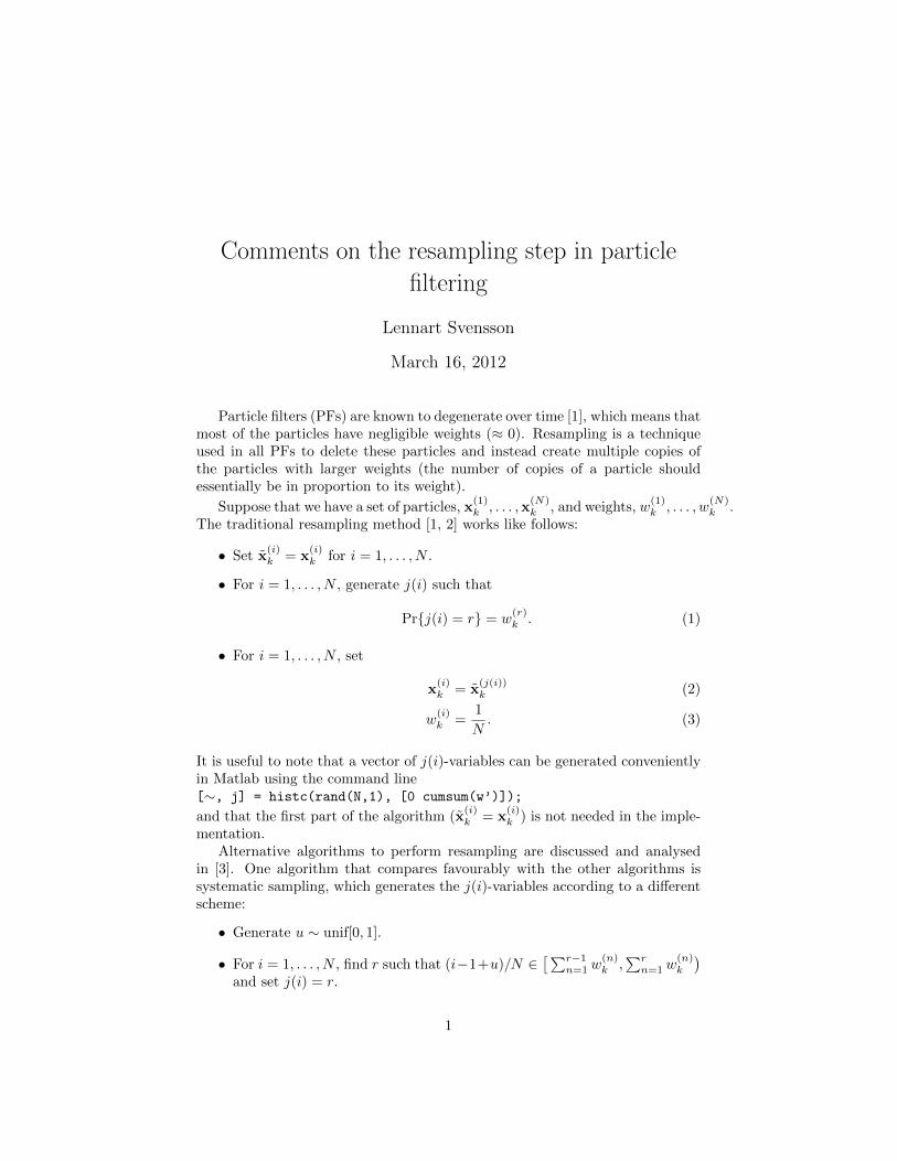
Though this may look more complicated it is actually a slightly faster algorithm,which can also be implemented conveniently in Matlab:[∼, j] = histc(rand(1)/N+0:1/N:(N-1)/N, [0 cumsum(w’)]);

However, since the complexity of both algorithms are O(N) (and really fast!),the benefits with systematic resampling are instead mainly a closer match be-tween the number of produced copies of a particle and its weight. Having saidthat, both algorithms work very well in practice and are asymptotically optimal,i.e., that the additional approximations imposed by the resampling step goes to0 as N →∞.

To understand why resampling inevitably leads to an approximation formost settings with small N , you may consider a simple example. Suppose

that you only have two particles (i.e., N = 2), with weights w(1)k = 0.2 and

w(2)k = 0.8. After resampling we will have two particles with weight 0.5 which

cannot represent the previous distribution. The best alternative may be tocreate two copies of the second particle though that means that (what used tobe) the first particle disappears in the resampling step.

References

[1] A. Doucet, S. Godsill, and C. Andrieu. On sequential monte carlo samplingmethods for bayesian filtering. Statistics and Computing, 10(3):197–208,2000.

[2] B. Ristic, S. Arulampalam, and N. Gordon. Beyond the Kalman filter :particle filters for tracking applications. Norwood, MA: Artech House, 2004.

[3] Jeroen D. Hol, Thomas B. Schon, and Fredrik Gustafsson. On resamplingalgorithms for particle filters. In Nonlinear Statistical Signal ProcessingWorkshop, Cambridge, United Kingdom, 2006.

2