Requirements Resources Bibliography - coastalsea.uk€¦ · 2.1 ASMITA OO software ... 2.3 Typical workflow to set-up new model ... concepts and methodology used in long-term morphological

ASMITA OO manual

Version 1.3, September 2016

i

Preface

The concept of an Aggregated Scale Morphological Interaction between Tidal basin and Adjacent

coast (ASMITA) was first proposed by Marcel Stive and co-workers at TU Delft. The first Matlab

version of ASMITA was developed by Tjerk Zitman at TU Delft. Work by Zheng Bing Wang and

colleagues also at TU Delft further developed the model and set out the basis of model

parameterisation. As part of the Estuaries Research Program Phase 2 (ERP2), funded by the

Environment Agency and Department for Environment, Food and Rural Affairs (part of project

FD2107) this research code was documented, tested and a manual prepared by Ian Townend and

Adrian Wright at ABPmer. Version 1.3 was released as Open Source software available from the

Estuary Guide web site (www.estuary-guide.net). Further developments were undertaken to add

additional elements and processes by Ian Townend, Jeremy Spearman, Kate Rossington and Michiel

Knappen at HR Wallingford. This manual details a new version that has an Object Oriented design

and was developed by Ian Townend at CoastalSEA in 2016.

Requirements

The code is written in MatlabTM and provided as Open Source code (issued under a GNU General

Public License). Routing within the model makes use of graph and directed graph functions which

were introduced in Matlab 2015b. There are however several versions of these functions available

from the Mathworks File Exchange if there is a need to use an earlier version of MatlabTM.

Resources

The zip file contains the following:

Matlab code and supporting files, sample models, and user manual.

Bibliography

Key papers setting out the theoretical background to the model include:

Stive, M.J.F., Capobianco, M., Wang, Z.B., Ruol, P., Buijsman, M.C., 1998. Morphodynamics of a

tidal lagoon and adjacent coast. In: J. Dronkers, M.B.A.M. Scheffers (Eds.). Physics of Estuaries and

Coastal Seas: 8th International Biennial Conference on Physics of Estuaries and Coastal Seas, 1996. A

A Balkema, pp. 397-407.

van Goor, M.A., Zitman, T.J., Wang, Z.B., Stive, M.J.F., 2003. Impact of sea-level rise on the

morphological equilibrium state of tidal inlets. Marine Geology, 202, 211-227.

Kragtwijk, N.G., Stive, M.J.F., Wang, Z.B., Zitman, T.J., 2004. Morphological response of tidal

basins to human interventions. Coastal Engineering, 51, 207-221.

Townend, I.H., Wang, Z.B., Stive, M.J.E., Zhou, Z., 2016a. Development and extension of an

aggregated scale model: Part 1 – Background to ASMITA. China Ocean Engineering, 30(4), 482-504.

Townend, I.H., Wang, Z.B., Stive, M.J.E., Zhou, Z., 2016b. Development and extension of an

aggregated scale model: Part 2 – Extensions to ASMITA. China Ocean Engineering, 30(5), 651-670.

Further sources of information are detailed in the References towards the end of the Manual.

http://www.estuary-guide.net/

ASMITA OO manual


ii

Contents

1 Introduction ..................................................................................................................................... 1

2 Getting Started ................................................................................................................................. 2

2.1 ASMITA OO software ............................................................................................................ 2

2.2 Opening ASMITA ................................................................................................................... 2

2.3 Typical workflow to set-up new model ................................................................................... 2

2.4 Parameter settings for sample models ..................................................................................... 5

3 Menus ............................................................................................................................................ 10

3.1 File ......................................................................................................................................... 10

3.2 Tools ...................................................................................................................................... 10

3.3 Project .................................................................................................................................... 11

3.4 Setup ...................................................................................................................................... 11

3.5 Run ........................................................................................................................................ 16

3.6 Plot ........................................................................................................................................ 16

4 Supporting Information for Model Setup ...................................................................................... 17

4.1 Model elements ..................................................................................................................... 17

4.2 Dispersion .............................................................................................................................. 19

4.3 Advection .............................................................................................................................. 20

4.4 Interventions .......................................................................................................................... 20

4.5 Saltmarsh ............................................................................................................................... 21

4.6 Storage ................................................................................................................................... 22

5 User functions................................................................................................................................ 22

5.1 AsmitaModel ......................................................................................................................... 22

5.2 UserPrismCoeffs ................................................................................................................... 22

5.3 UserSLRrate .......................................................................................................................... 23

5.4 UserUnitTesting .................................................................................................................... 23

6 Program Structure.......................................................................................................................... 23

7 Additional References ................................................................................................................... 24

Appendix A – Function call sequence in RunModel ............................................................................. 26

Appendix B – UML Class diagrams ..................................................................................................... 28

ASMITA OO manual


1

1 Introduction Aggregated Scale Morphological Interaction between a Tidal inlet and the Adjacent coast (ASMITA).

This manual has been written as a guide to using the Matlab ASMITA model and illustrates the

concepts and methodology used in long-term morphological modelling.

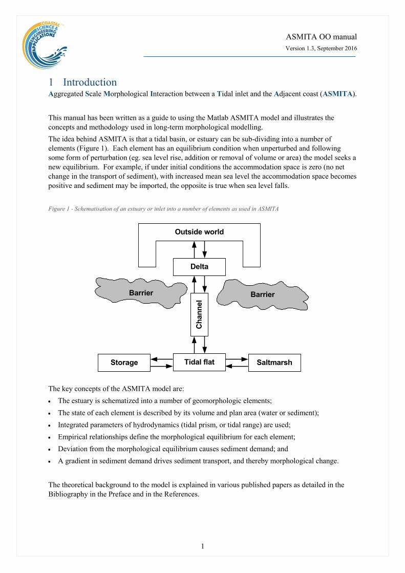
The idea behind ASMITA is that a tidal basin, or estuary can be sub-dividing into a number of

elements (Figure 1). Each element has an equilibrium condition when unperturbed and following

some form of perturbation (eg. sea level rise, addition or removal of volume or area) the model seeks a

new equilibrium. For example, if under initial conditions the accommodation space is zero (no net

change in the transport of sediment), with increased mean sea level the accommodation space becomes

positive and sediment may be imported, the opposite is true when sea level falls.

Figure 1 - Schematisation of an estuary or inlet into a number of elements as used in ASMITA

The key concepts of the ASMITA model are:

The estuary is schematized into a number of geomorphologic elements;

The state of each element is described by its volume and plan area (water or sediment);

Integrated parameters of hydrodynamics (tidal prism, or tidal range) are used;

Empirical relationships define the morphological equilibrium for each element;

Deviation from the morphological equilibrium causes sediment demand; and

A gradient in sediment demand drives sediment transport, and thereby morphological change.

The theoretical background to the model is explained in various published papers as detailed in the

Bibliography in the Preface and in the References.

Barrier Barrier

Delta

Ch

an

nel

Tidal flat

Outside world

Storage Saltmarsh

ASMITA OO manual


2

2 Getting Started

2.1 ASMITA OO software The ASMITA software has been written using the software language Matlab, version 2015/16. The

software utilises only core Matlab functions and does not use any toolboxes. Section 6 of this manual

provides details of the program structure, including the class diagram, function call and related

information that will be of use to those who wish to develop the software, or explore alternative model

parameterisations. To support this, a number of functions have been written as standalone (i.e. not

contained within the class code file) to allow the user to modify aspects of the model behaviour. These

are detailed in Section 5.

2.2 Opening ASMITA A graphical user interface (GUI) is used to set-up, run scenarios, plot results and export model output.

With the Matlab working directory (folder) pointing to the folder containing the ASMITA code, the

GUI is run from the command prompt by typing:

>> Asmita.Gui;

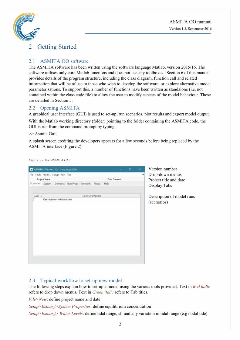
A splash screen crediting the developers appears for a few seconds before being replaced by the

ASMITA interface (Figure 2).

Figure 2 - The ASMITA GUI

Version number

Drop-down menus

Project title and date

Display Tabs

Description of model runs

(scenarios)

2.3 Typical workflow to set-up new model The following steps explain how to set-up a model using the various tools provided. Text in Red italic

refers to drop down menus. Text in Green italic refers to Tab titles.

File>New: define project name and date

Setup>Estuary>System Properties: define equilibrium concentration

Setup>Estuary> Water Levels: define tidal range, slr and any variation in tidal range (e.g nodal tide)

ASMITA OO manual


3

Setup>Element>Define Elements: specify how many elements of each type are needed

Setup>Element>Element Properties: define volume, area etc for each element

Setup>Run Parameters>Time Step: define time step and length of run

Setup>Run Parameters>Equilibrium Coefficients: select equilibrium prism coefficient set from list

(coefficients are defined in UserPrismCoeffs.m – see Section 5.2 for further details).

Setup>Estuary>Dispersion: define the horizontal exchange between elements. The direction from-to

working landwards from the most seaward element is important as this is used to calculate the tidal

prism in each reach.

River flow, Interventions, Littoral Drift, Saltmarsh, Tidal Pumping and various constraints can be

added as required. However, the above is the minimum required for the model to run.

To examine what has been set-up the Tabs provide a summary of what is currently defined. Note:

these only update when clicked on using a mouse and the values cannot be edited from the Tabs.

Scenarios: lists the cases that have been run with a case id and description.

System: tabulates the system properties and flags that have been set (display only).

Elements: tabulates the key properties of each element (display only).

Run Props: tabulates the key run conditions and equilibrium coefficients (display only).

Network: graphic of the element network showing the connectivity and horizontal exchanges between

all elements (m3/s).

Flows: graphic of the elements that have an advection (e.g. channels) showing the connectivity and the

flow rate (m3/s).

Response: summary of morphological response times based on system definition.

Help: an abridged version of this workflow guide.

Figure 3 – Tabs in Main GUI

ASMITA OO manual


4

Adding a river flow:

Setup>River: define channel element that river flows into, flow rate and sediment concentration

Setup>Estuary>Advection: define how the river flows through the model. Again this is specified as

from-to and the total flow into any element must equal the flow out.

Setup>Run Parameters>Conditions: check the flag for River flow offset, if you want the flow to be

accounted for in the initial condition.

Note: river flows can also be added and edited in the Advection definition table but this still requires

the concentration of any sediment load to defined using the Setup>River user interface.

Adding interventions:

Setup>Interventions: select element and define the years in which there is a change. Positive is an

increase in water volume or surface area.

Setup>Run Parameters>Conditions: check flag to include interventions. (Note that once interventions

have been defined, they can be included or omitted by using this flag).

To run the model:

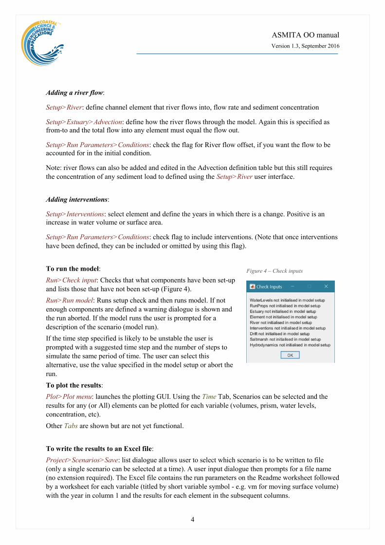
Run>Check input: Checks that what components have been set-up

and lists those that have not been set-up (Figure 4).

Run>Run model: Runs setup check and then runs model. If not

enough components are defined a warning dialogue is shown and

the run aborted. If the model runs the user is prompted for a

description of the scenario (model run).

If the time step specified is likely to be unstable the user is

prompted with a suggested time step and the number of steps to

simulate the same period of time. The user can select this

alternative, use the value specified in the model setup or abort the

run.

To plot the results:

Plot>Plot menu: launches the plotting GUI. Using the Time Tab, Scenarios can be selected and the

results for any (or All) elements can be plotted for each variable (volumes, prism, water levels,

concentration, etc).

Other Tabs are shown but are not yet functional.

To write the results to an Excel file:

Project>Scenarios>Save: list dialogue allows user to select which scenario is to be written to file

(only a single scenario can be selected at a time). A user input dialogue then prompts for a file name

(no extension required). The Excel file contains the run parameters on the Readme worksheet followed

by a worksheet for each variable (titled by short variable symbol - e.g. vm for moving surface volume)

with the year in column 1 and the results for each element in the subsequent columns.

Figure 4 – Check inputs

ASMITA OO manual


5

2.4 Parameter settings for sample models The zip file includes some sample models as *.mat files. The parameters needed to run the models are

saved in these files (along with any scenarios that have been run).

2.4.1 Humber Model (simple 3 element model: delta-channel-flat)

The settings used in the Humber3EM model are as follows:

Setup>Estuary>System Properties: Coarse Fraction Equilibrium Concentration = 0.72 kg/m3. Fine

fraction value is the same in this example (see Section 2.4.3 for details of how to introduce mixed

sediments).

Setup>Estuary> Water Levels>Tidal Range = 5.84 m (at mouth)

Setup>Estuary> Water Levels>LW/HW amplitude ratio = 1 if the tidal signal (or related cycles) is not

symmetric about mean tide level, this ratio allows an adjustment to be made (the default is 1).

Setup>Estuary> Water Levels>Mean Sea Level at t=0 = 0 m. Allows for any offset of MSL to the

local datum used for elevations.

Setup>Estuary> Water Levels>Rate of sea level rise = 0.0018 m/year

Setup>Estuary> Water Levels>Number of Cycles = 2

The next three fields can have multiple values to include the number of cycles specified

Setup>Estuary> Water Levels>Amplitude = 0.1 0.04 m

Setup>Estuary> Water Levels>Period = 18.6 180 years.

Setup>Estuary> Water Levels>Phase = 12.2 128 years. Defines the offset to give the correct timing

of each cycle in the Julian calendar.

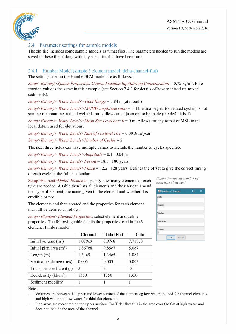
Setup>Element>Define Elements: specify how many elements of each

type are needed. A table then lists all elements and the user can amend

the Type of element, the name given to the element and whether it is

erodible or not.

The elements and then created and the properties for each element

must all be defined as follows:

Setup>Element>Element Properties: select element and define

properties. The following table details the properties used in the 3

element Humber model:

Channel Tidal Flat Delta

Initial volume (m3) 1.079e9 3.97e8 7.719e8

Initial plan area (m2) 1.867e8 9.85e7 5.0e7

Length (m) 1.34e5 1.34e5 1.0e4

Vertical exchange (m/s) 0.003 0.003 0.003

Transport coefficient (-) 2 2 -2

Bed density (kb/m3) 1350 1350 1350

Sediment mobility 1 1 1

Notes:

Volumes are between the upper and lower surface of the element eg low water and bed for channel elements

and high water and low water for tidal flat elements

Plan areas are measured on the upper surface. For Tidal flats this is the area over the flat at high water and

does not include the area of the channel.

Figure 5 – Specify number of

each type of element

ASMITA OO manual


6

Length is the along channel length of the element

Vertical exchange and Transport coefficient are determined as explained in Townend et al (2016). The

Transport coefficient for the Delta is negative because the equilibrium condition of this type of element is in

terms of sediment volume whereas the others are all in terms of water volume.

Bed density is a representative density for the bed in each element.

Sediment mobility is only used when tidal pumping is included to adjust the along channel concentrations.

Setup>Run Parameters>Time Step>Time Step = 0.5 (years)

Setup>Run Parameters>Time Step>Number of Time Steps = 640 (i.e. 320 years)

Setup>Run Parameters>Time Step>Output Interval = 2 (i.e. every other time step)

Setup>Run Parameters>Time Step>Start Year = 1703 (default is zero and only needed if doing a

historical hindcast. However, any Interventions must be defined relative to the same time frame)

Setup>Run Parameters>Equilibrium Coefficients: select ‘Default’

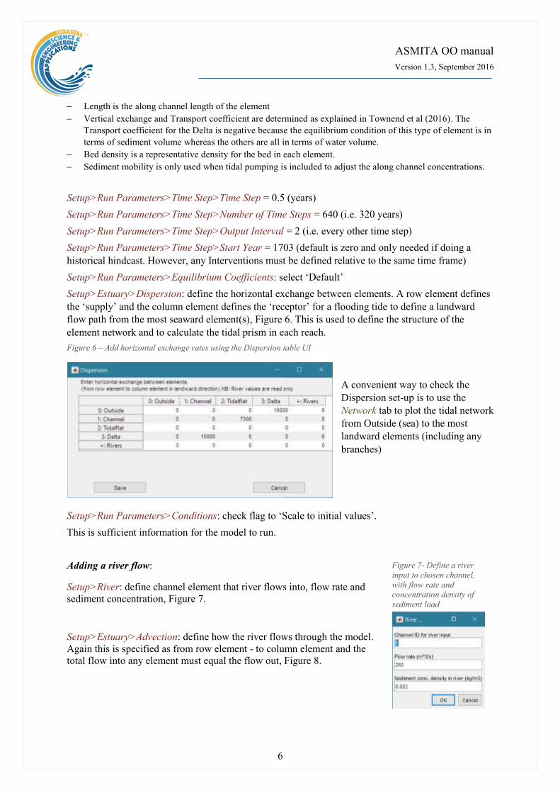
Setup>Estuary>Dispersion: define the horizontal exchange between elements. A row element defines

the ‘supply’ and the column element defines the ‘receptor’ for a flooding tide to define a landward

flow path from the most seaward element(s), Figure 6. This is used to define the structure of the

element network and to calculate the tidal prism in each reach.

Figure 6 – Add horizontal exchange rates using the Dispersion table UI

A convenient way to check the

Dispersion set-up is to use the

Network tab to plot the tidal network

from Outside (sea) to the most

landward elements (including any

branches)

Setup>Run Parameters>Conditions: check flag to ‘Scale to initial values’.

This is sufficient information for the model to run.

Adding a river flow:

Setup>River: define channel element that river flows into, flow rate and

sediment concentration, Figure 7.

Setup>Estuary>Advection: define how the river flows through the model.

Again this is specified as from row element - to column element and the

total flow into any element must equal the flow out, Figure 8.

Figure 7- Define a river

input to chosen channel,

with flow rate and

concentration density of

sediment load

ASMITA OO manual


7

Figure 8 – Add advection flow rates using the Advection Table UI

A convenient way to check the

Advection set-up is to use the Flow

tab to plot the flow network from

Source (river or rivers) to Outside

(sea).

Setup>Run Parameters>Conditions: check the flag for ‘River flow offset’, if you want the flow to be

accounted for in the initial condition.

Adding interventions:

Setup>Interventions: select element from list table and use

the table UI to define the years in which there is a change,

Figure 9Figure 9. Positive is an increase in water volume or

surface area.

Setup>Run Parameters>Conditions: check flag to include

interventions, Figure 10. (Note that once interventions have

been defined, they can be included or omitted from an

individual model by using this flag, but remain saved in the

model set-up).

Figure 10 – Conditions UI allows conditions and constraints to be included

or omitted from model run

Figure 9 - Define interventions by year, volume

change and plan area change. Use add row to

include additional changes

ASMITA OO manual


8

2.4.2 Venice model (multiple inlets and saltmarsh)

The steps to setup the model follows those outlined above. The main differences here are the addition

of multiple inlets which are defined using the Dispersion and Advection parameters and the inclusion

of saltmarsh. The following summarises the settings used in the Venice 9EM model and details the

additional steps to setup the model.

Setup>Estuary>System Properties: Coarse Fraction Equilibrium Concentration = 0.04 kg/m3.


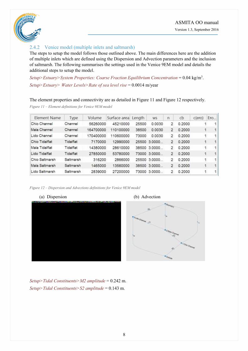
The element properties and connectivity are as detailed in Figure 11 and Figure 12 respectively.

Figure 11 – Element definitions for Venice 9EM model

Figure 12 – Dispersion and Advections definitions for Venice 9EM model

(a) Dispersion

(b) Advection

Setup>Tidal Constituents>M2 amplitude = 0.242 m.

Setup>Tidal Constituents>S2 amplitude = 0.143 m.

ASMITA OO manual


9

Setup>Saltmarsh>Species Parameters

The user interface to enter the saltmarsh parameters allows the user to

enter multiple species values with values separated by a space as

illustrated in Figure 13 (applies to minimum depth, maximum depth,

Maximum biomass and Species productivity). Further explanation of the

saltmarsh parameters is given in Section 4.5.

Note: edge erosion is only applicable when using variable surface areas

Not available in version 1.3

Setup>Run Parameters>Conditions: check the flag to ‘Include saltmarsh biomass’. If the flag is not

checked, the model treats the saltmarsh element like any other element and uses the prism based

relationship to define the equilibrium volumes (see Section 5.2).

Setup>Run Parameters>Equilibrium Coefficients: select ‘Venice’.

2.4.3 Amelander model (mixed sediments)

This model is used to explore the influence of introducing variable bed density and mixed (fine and

course sediments. The original model was detailed in van Goor et al. (2003). This model was revisited

to consider the influence of fine sediment in Wang et al. (2014) and extended to consider the

combined influence of mixed sediment and bed density in Townend et al. (2016b). The file provided

has the parameters setup for case (vi) in Table 2 of Townend et al. and the various cases listed in

Table 2 have already been run and saved in the model.

Setup>Estuary>System Properties: Coarse Fraction Equilibrium Concentration = 0.64 kg/m3.

Setup>Estuary>System Properties: Fine Fraction Equilibrium Concentration = 0.2 kg/m3.

The element properties and connectivity are as detailed in Figure 14. The dispersions are simply 300,

300, 10,000 as the exchanges from Outside to Delta, Delta to Channel and Channel to Tidalflat

respectively.

Figure 14- Element definitions for Amelander 3EM model

Figure 13 – Define saltmarsh

species and enhanced settling

parameters

ASMITA OO manual


10


Setup>Run Parameters>Equilibrium Coefficients: select ‘Amelander’.

2.4.4 Severn model (tidal pumping)

This model illustrates the inclusion of tidal pumping. The set up procedure is similar to that used for

the Humber (Section 2.4.1). The only addition is to set the condition to include tidal pumping. For this

this to be meaningful, the channel needs to be sub-divided into a number of elements (6 are used in

this case). The model also shows the use of multiple tidal flats linked to each channel reach (one for

each side of the estuary). This can be useful for illustrating change but the dynamics of the model are

the same if a single tidal flat is used for each reach (assuming the properties are the same for each pair

of flats). This model also allows the plotting of variations along the channel using the Distance and

XYZ tabs in the plot GUI, as illustrated in Figure 15.

Figure 15 – Plots from Severn model showing along channel variation at a point in time and as space-time surface

3 Menus

3.1 File File>New: clears any existing model (prompting to save if not already saved) and a popup dialog box

prompts for Project name and Date (default is current date).

File>Open: existing Asmita models are saved as *.mat files. User selects a model from dialog box.

File>Save: save a file that has already been saved.

File>Save as: save a file with a new or different name.

File>Exit: exit the program. The close window button has the same effect.

3.2 Tools Tools>Refresh: updates Scenarios tab.

Tools>Clear all>Model: deletes the current model.

Tools>Clear all>Figures: deletes all results plot figures (useful if a large number of plots have been

produced).

Tools>Clear all>Scenarios: deletes all scenarios listed on the Scenarios tab but does not affect the

model setup.

ASMITA OO manual


11

3.3 Project Project>Definition: edit the Project name and Date

Project>Scenarios>Edit: table listing of scenario descriptions allowing the user to edit individual

descriptions.

Project>Scenarios>Save: user selects the scenario to be saved from a list box of scenarios and the is

then prompted to name the file. The full details of the model setup and the results are written to an

Excel spreadsheet.

Project>Scenarios>Delete: user selects the scenario to be deleted from a list box of scenarios and

results are then deleted (model setup is not changed).

3.4 Setup The setup menu provides a series of menus to enable different components of the model to be defined.

Setup>Estuary>System Properties:

Define the concentration that is target or global equilibrium

concentration. These should be the same value if only a single

fraction is being considered.

The e-folding length is the rate of width convergence and is used if

tidal pumping is included

Wind speed and the elevation at which the wind is measured are used

in the 3D estuary form model to

account for internal wave action (not

implemented in version 1.3)

Setup>Estuary>Water Levels:

Tidal range and period are defined at the entrance to estuary, or inlet

The LW/HW amplitude ratio accounts for any difference in the

amplitude to low water and high water relative to the define mean sea

level1. Used to adjust influence of changes in tidal range.

The mean sea level at the start of the model run (allows for offsets from

zero datum).

Rate of sea level rise as a linear rate (positive or negative). See Section

5.3 for alternatives.

Number of cycles to be included that vary the tidal range as a function

of time. The number of entries for amplitude, period and phase have to

agree with the number of cycles specified. The phase defines a shift in

the cycle to align with the Julian calendar. This is only or relevance if

the model is being used to hindcast change and compare volume

changes with observed changes (e.g. Townend et al., 2007).

1 Option included because of observed bias (eg on Humber nodal tidal cycle has an amplitude of 0.23m with a

high water amplitude of ~0.14 and low water amplitude of ~0.08; i.e. ratio = 0.08/0.14 =0.57). The default value

is 1.

ASMITA OO manual


12

Setup>Estuary>Dispersion:

Define the horizontal exchange between

elements (m/s). Exchanges proceed from the

most seaward element(s) in a landwards

direction. Values are entered in the cell which

is from a row element going to a column

element (e.g. from row Delta to column

Channel). These are used to determine the

network connectivity and the resultant network

can be viewed on the Network tab. For detail

of how to estimate appropriate values for the

horizontal exchange see Wang et al. (2008) or

Townend et al. (2016a).

Setup>Rivers>River advection:

Define the advective flows through the channel

network (m3/s). For river flows, these are

defined from the River source to the Outside

(the open coast). Values are entered in the cell

which is from a row element going to a column

element (e.g. from Delta to Outside). There

should be a mass balance in and out of any

element and along the flow path(s) from

Source(s) to the Outside. This is checked when

the channel flow network is viewed on the

Flow tab.

The sediment concentrations associated with the river inputs are defined in Setup>Rivers>River

inputs. If a new river flow is added in the Advection table, a River object is added and the user is

prompted to use the Setup>Rivers>River inputs component to add the sediment concentration.

A river input with a sediment load that is not equal to the coarse grain equilibrium concentration will

act as a perturbation to the model (a forced change). To avoid this there is an option to include the

advective flows in the Setup>Run Parameters>Conditions: by setting the ‘River flow offset’ check

box. The details of this are explained in discussion on advective flows in Townend et al. (2016a).

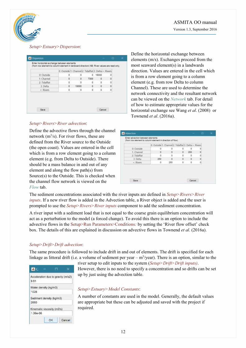
Setup>Drift>Drift advection:

The same procedure is followed to include drift in and out of elements. The drift is specified for each

linkage as littoral drift (i.e. a volume of sediment per year – m3/year). There is an option, similar to the

river setup to edit inputs to the system (Setup>Drift>Drift inputs).

However, there is no need to specify a concentration and so drifts can be set

up by just using the advection table.

Setup>Estuary>Model Constants:

A number of constants are used in the model. Generally, the default values

are appropriate but these can be adjusted and saved with the project if

required.

ASMITA OO manual


13

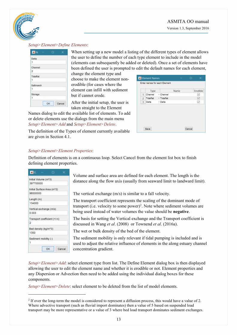
Setup>Element>Define Elements:

When setting up a new model a listing of the different types of element allows

the user to define the number of each type element to include in the model

(elements can subsequently be added or deleted). Once a set of elements have

been defined the user is prompted to edit the default names for each element,

change the element type and

choose to make the element non-

erodible (for cases where the

element can infill with sediment

but if cannot erode.

After the initial setup, the user is

taken straight to the Element

Names dialog to edit the available list of elements. To add

or delete elements use the dialogs from the main menu

Setup>Element>Add and Setup>Element>Delete.

The definition of the Types of element currently available

are given in Section 4.1.

Setup>Element>Element Properties:

Definition of elements is on a continuous loop. Select Cancel from the element list box to finish

defining element properties.

Volume and surface area are defined for each element. The length is the

distance along the flow axis (usually from seaward limit to landward limit).

The vertical exchange (m/s) is similar to a fall velocity.

The transport coefficient represents the scaling of the dominant mode of

transport (i.e. velocity to some power)2. Note where sediment volumes are

being used instead of water volumes the value should be negative.

The basis for setting the Vertical exchange and the Transport coefficient is

discussed in Wang et al. (2008) or Townend et al. (2016a).

The wet or bulk density of the bed of the element.

The sediment mobility is only relevant if tidal pumping is included and is

used to adjust the relative influence of elements in the along estuary channel

concentration gradient.

Setup>Element>Add: select element type from list. The Define Element dialog box is then displayed

allowing the user to edit the element name and whether it is erodible or not. Element properties and

any Dispersion or Advection then need to be added using the individual dialog boxes for these

components.

Setup>Element>Delete: select element to be deleted from the list of model elements.

2 If over the long-term the model is considered to represent a diffusion process, this would have a value of 2.

Where advective transport (such as fluvial import dominates) then a value of 5 based on suspended load

transport may be more representative or a value of 3 where bed load transport dominates sediment exchanges.

ASMITA OO manual


14

Setup>Saltmarsh>Species parameters:

Any number of saltmarsh species can be entered and a check is made to

ensure that the number of values entered for minimum depth, maximum

depth maximum biomass and species productivity is consistent with the

number of species specified.

Coefficients for biomass dependent enhanced settling rate

Minimum and maximum marsh edge erosion rates due to wave action.

These are only used when variable surface area is included. Not available

in version 1.3.

Setup>Saltmarsh>Equilibrium marsh depth:

This utility allows the user to explore the response of the marsh depth to the defined saltmarsh

parameters and to see how this response varies by adjusting the biomass production rates for each of

the species included. On selecting this option, a dialog box presents

the currently defined values of the biomass production rates and the

user has the option to change these. [This does not alter the values

saved in the model.] Three plots are then presented in a single figure.

These show the average

concentration the proportion of time

submerged for the intertidal flat as a

whole (top left) and the marsh

surface (bottom left). The plot to the

right then shows how the equilibrium

depth and the equilibrium production

of the marsh vary as a function of sea

level rise. The dashed lines highlight

the values for the rate of sea level

rise defined in the model. For further

discussion of the saltmarsh model

and the bio-morphological response,

see Townend et al. (2010).

ASMITA OO manual


15

Setup>Rivers>River inputs: This component can only be added once some channel elements have

been setup in the model. If no rivers are defined, the dialog box requires the Channel id number, along

with the flow rate and the concentration density of the rivers sediment

load. If one or more rivers have already been added, a list box prompts

the user to select from a list of channels with river inputs or to Add a

river.

To remove an input, use Setup>Rivers>Delete input and select the

source to be deleted from the list of channels with river inputs.

River flows can also be defined in the Setup>Rivers>River advection

table but it is still necessary to add the Sediment concentration using the

Setup>Rivers>River inputs dialog box.

Once Advection throughout the network has been defined the flow routes can be checked using the

Flow tab.

Setup>Littoral Drift: Littoral drift is much the same way as river flows, except that a mass balance is

not imposed. The source or inputs of drift can be defined as a drift rate (m3/year) using Setup>Littoral

Drift>Drift inputs. However, there is no need to assign a concentration to the drift. The flow through

the system is then defined using the advection table Setup>Littoral Drift>Drift advection, in the same

way as for river flows. Drift inputs can be removed using Setup>Littoral Drift>Delete input.

Setup>Tidal Constituents:

Selected tidal constituents may be needed for certain model components.

The model currently assumes a semi-diurnal tide and the M2 and S2

amplitudes are used to estimate the concentration over the marsh and the

submergence time if Saltmarshes are included in the model.

The M4 amplitude and phase are used to estimate the influence of the over-

tide in the tidal pumping component

Setup>Interventions>: select element from list of

elements and then use table to add interventions.

Selection of elements is in a continuous loop.

Select Cancel from the element list box to finish

adding interventions. Define the Year of the

intervention (this must be consistent with the

Start Year and duration of the model run defined

in Setup>Run Parameters>Time step). The

Volume and Surface Area are the changes in

water volume and element plan area respectively.

Use negative values to represent reductions (e.g.

due to a reclamation).

ASMITA OO manual


16

In order for the defined interventions to be included in the model run the Include Interventions

condition needs to be set. This allows runs to be made with and without the interventions, without the

need to redefine them each time.

Setup>Run Parameters>Conditions: check the flag to ‘Include Interventions’.

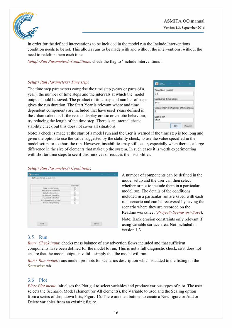
Setup>Run Parameters>Time step:

The time step parameters comprise the time step (years or parts of a

year), the number of time steps and the intervals at which the model

output should be saved. The product of time step and number of steps

gives the run duration. The Start Year is relevant where and time

dependent components are included that have used Years defined in

the Julian calendar. If the results display erratic or chaotic behaviour,

try reducing the length of the time step. There is an internal check

stability check but this does not cover all situations.

Note: a check is made at the start of a model run and the user is warned if the time step is too long and

given the option to use the value suggested by the stability check, to use the value specified in the

model setup, or to abort the run. However, instabilities may still occur, especially when there is a large

difference in the size of elements that make up the system. In such cases it is worth experimenting

with shorter time steps to see if this removes or reduces the instabilities.

Setup>Run Parameters>Conditions:

A number of components can be defined in the

model setup and the user can then select

whether or not to include them in a particular

model run. The details of the conditions

included in a particular run are saved with each

run scenario and can be recovered by saving the

scenario where they are recorded on the

Readme worksheet (Project>Scenarios>Save).

Note: Bank erosion constraints only relevant if

using variable surface area. Not included in

version 1.3

3.5 Run Run> Check input: checks mass balance of any advection flows included and that sufficient

components have been defined for the model to run. This is not a full diagnostic check, so it does not

ensure that the model output is valid – simply that the model will run.

Run> Run model: runs model, prompts for scenarios description which is added to the listing on the

Scenarios tab.

3.6 Plot Plot>Plot menu: initialises the Plot gui to select variables and produce various types of plot. The user

selects the Scenario, Model element (or All elements), the Variable to used and the Scaling option

from a series of drop down lists, Figure 16. There are then buttons to create a New figure or Add or

Delete variables from an existing figure.

ASMITA OO manual


17

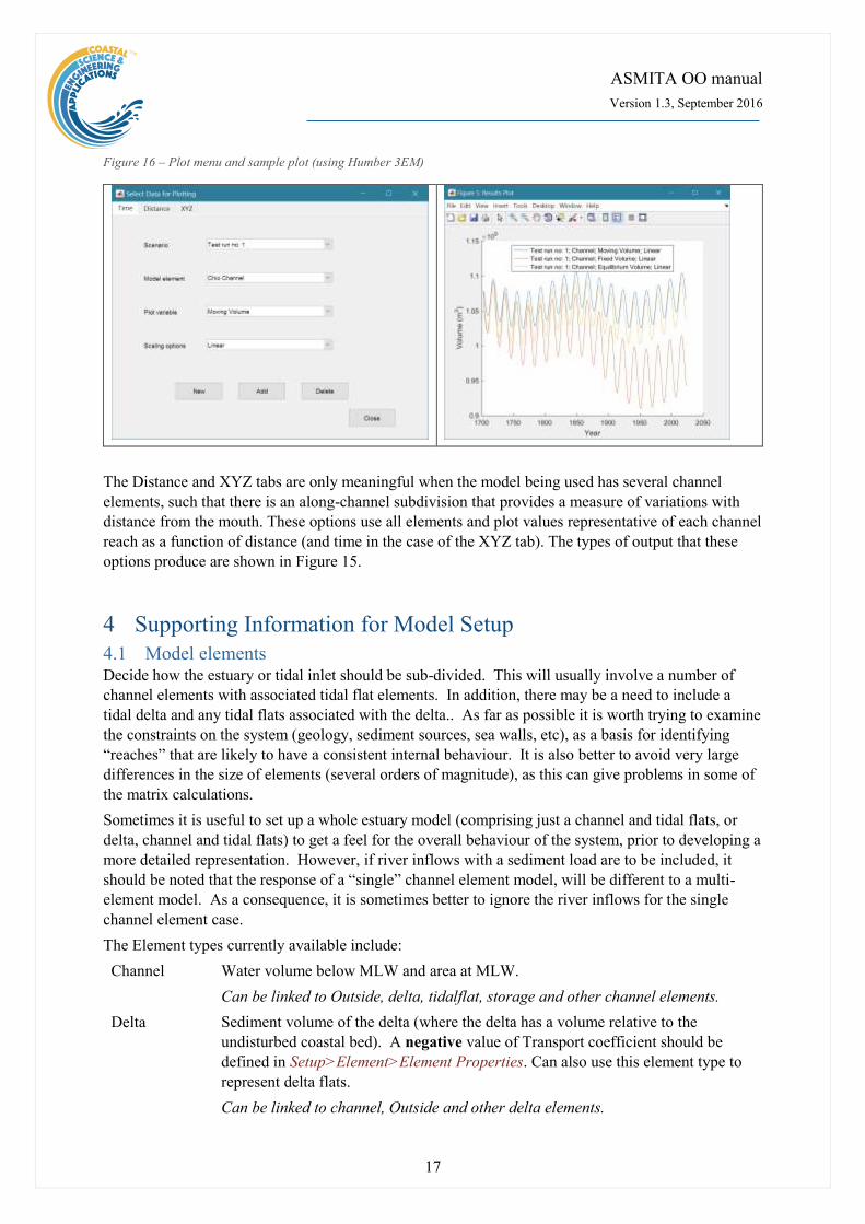
Figure 16 – Plot menu and sample plot (using Humber 3EM)

The Distance and XYZ tabs are only meaningful when the model being used has several channel

elements, such that there is an along-channel subdivision that provides a measure of variations with

distance from the mouth. These options use all elements and plot values representative of each channel

reach as a function of distance (and time in the case of the XYZ tab). The types of output that these

options produce are shown in Figure 15.

4 Supporting Information for Model Setup

4.1 Model elements Decide how the estuary or tidal inlet should be sub-divided. This will usually involve a number of

channel elements with associated tidal flat elements. In addition, there may be a need to include a

tidal delta and any tidal flats associated with the delta.. As far as possible it is worth trying to examine

the constraints on the system (geology, sediment sources, sea walls, etc), as a basis for identifying

“reaches” that are likely to have a consistent internal behaviour. It is also better to avoid very large

differences in the size of elements (several orders of magnitude), as this can give problems in some of

the matrix calculations.

Sometimes it is useful to set up a whole estuary model (comprising just a channel and tidal flats, or

delta, channel and tidal flats) to get a feel for the overall behaviour of the system, prior to developing a

more detailed representation. However, if river inflows with a sediment load are to be included, it

should be noted that the response of a “single” channel element model, will be different to a multi-

element model. As a consequence, it is sometimes better to ignore the river inflows for the single

channel element case.

The Element types currently available include:

Channel Water volume below MLW and area at MLW.

Can be linked to Outside, delta, tidalflat, storage and other channel elements.

Delta Sediment volume of the delta (where the delta has a volume relative to the

undisturbed coastal bed). A negative value of Transport coefficient should be

defined in Setup>Element>Element Properties. Can also use this element type to

represent delta flats.

Can be linked to channel, Outside and other delta elements.

ASMITA OO manual


18

Tidalflat Water volume between MLW and MHW over flats (i.e. not including the prism

over the channel) and area over flats. Flats on both sides of channel in a given

reach can be included in a single flat element. This element can also be defined as

a sediment volume by defining a negative value of Transport coefficient in

Setup>Element>Element Properties.

Can be linked to any element within the inlet or estuary.

Saltmarsh Water volume over the marsh and associated area. Saltmarsh on both sides of a

channel in a given reach can be included in a single saltmarsh element. Can also be

used to represent an upper tidal flat by not setting the Include Saltmarsh condition

in Setup>Run Parameters>Conditions.

Can be linked to any element within the inlet or estuary.

Storage Water volume and area of storage unit. Treated as locally independent of system

(not dependent on upstream prism) but contributing to downstream prism.

Can be linked to any element within the inlet or estuary but should not have any

‘upstream’ elements.

Using a suitable DGM the volumes and areas can be calculated in one of two ways:

(i) Define a horizontal plane at high and low water level and calculate the water volumes below

the plane and the surface areas on the planes.

(ii) Use the surfaces for high and low water derived from a hydraulic model in conjunction with a

DGM to calculate the water volumes below the surface and the surface areas at high and low water.

This added complexity is not needed for small or relatively short estuaries but can be important for

longer estuaries that are near resonant (Thames, Humber, Severn, etc).

It is also possible to define elements as sediment volumes rather than wet volumes. If this is preferred,

then the sediment transport coefficient, n, should be expressed as a negative value. This was the basis

for the original model development which used fixed surface areas (Kragtwijk et al., 2004; Stive et al.,

1998) and works for this form of configuration.

The bulk density of sediment relates to the density of the bed within the element. This is included to

take account of the consolidation of sediment that is deposited and is used in the code to adjust the

vertical rate of exchange. The default value of 1350kg.m-3 is typical for many UK estuaries.

The sediment transport coefficient reflects the nature of the transport process. For simple diffusion a

value of 2 can be adopted. Where bed or suspended transport dominate a value between 3 and 5 may

be more appropriate. As this model is considering long-term evolution it can be argued that the

process can be treated as essentially diffusive, suggesting a value of 2. Furthermore, it is the product

of n and cE that determines the morphological response time, so that using a set value may simply

result in a slightly different value of cE.

The vertical exchange (although not strictly a sediment fall velocity) should be based on the fall

velocity for the sediment type that characterises most of the element. There is an inter-dependence

between the fall velocity and the horizontal exchange which is explained further in the Section on

Dispersion.

ASMITA OO manual


19

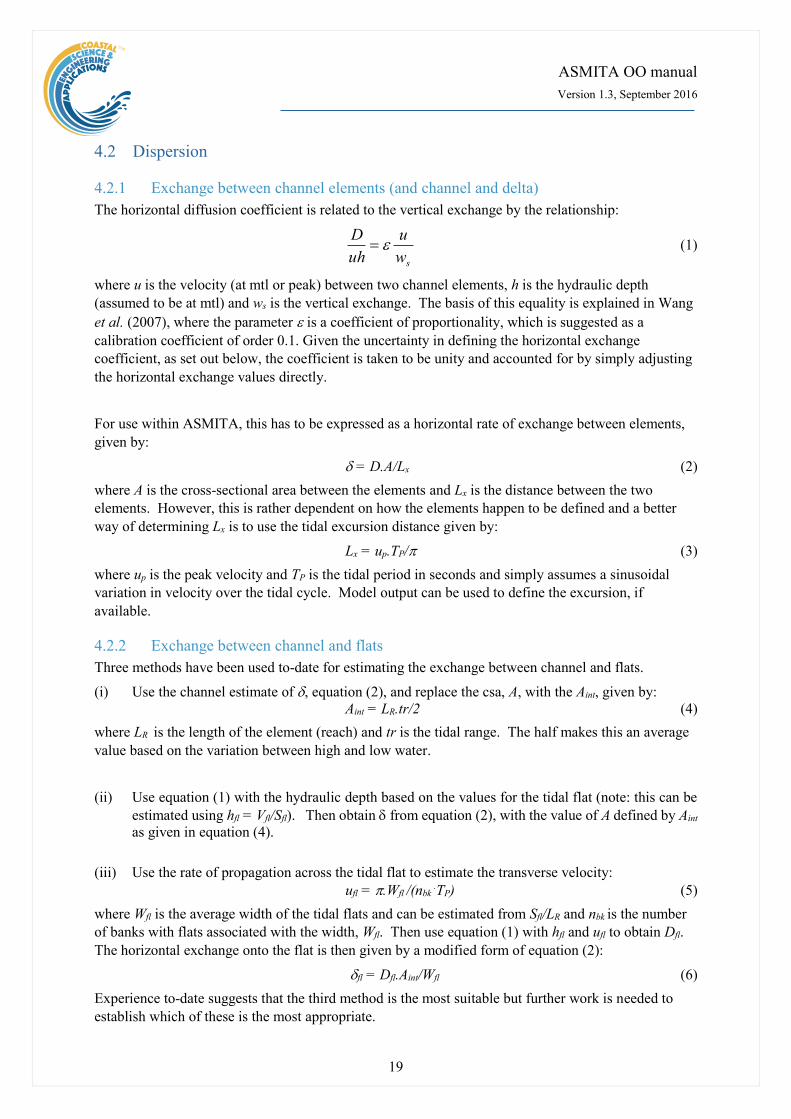
4.2 Dispersion

4.2.1 Exchange between channel elements (and channel and delta)

The horizontal diffusion coefficient is related to the vertical exchange by the relationship:

sw

u

uh

D (1)

where u is the velocity (at mtl or peak) between two channel elements, h is the hydraulic depth

(assumed to be at mtl) and ws is the vertical exchange. The basis of this equality is explained in Wang

et al. (2007), where the parameter is a coefficient of proportionality, which is suggested as a

calibration coefficient of order 0.1. Given the uncertainty in defining the horizontal exchange

coefficient, as set out below, the coefficient is taken to be unity and accounted for by simply adjusting

the horizontal exchange values directly.

For use within ASMITA, this has to be expressed as a horizontal rate of exchange between elements,

given by:

= D.A/Lx (2)

where A is the cross-sectional area between the elements and Lx is the distance between the two

elements. However, this is rather dependent on how the elements happen to be defined and a better

way of determining Lx is to use the tidal excursion distance given by:

Lx = up.TP/ (3)

where up is the peak velocity and TP is the tidal period in seconds and simply assumes a sinusoidal

variation in velocity over the tidal cycle. Model output can be used to define the excursion, if

available.

4.2.2 Exchange between channel and flats

Three methods have been used to-date for estimating the exchange between channel and flats.

(i) Use the channel estimate of , equation (2), and replace the csa, A, with the Aint, given by:

Aint = LR.tr/2 (4)

where LR is the length of the element (reach) and tr is the tidal range. The half makes this an average

value based on the variation between high and low water.

(ii) Use equation (1) with the hydraulic depth based on the values for the tidal flat (note: this can be

estimated using hfl = Vfl/Sfl). Then obtain from equation (2), with the value of A defined by Aint

as given in equation (4).

(iii) Use the rate of propagation across the tidal flat to estimate the transverse velocity:

ufl = .Wfl /(nbk .TP) (5)

where Wfl is the average width of the tidal flats and can be estimated from Sfl/LR and nbk is the number

of banks with flats associated with the width, Wfl. Then use equation (1) with hfl and ufl to obtain Dfl.

The horizontal exchange onto the flat is then given by a modified form of equation (2):

fl = Dfl.Aint/Wfl (6)

Experience to-date suggests that the third method is the most suitable but further work is needed to

establish which of these is the most appropriate.

ASMITA OO manual


20

4.3 Advection The model provides for advective flows through the system. Necessarily the flow in and out of an

element must sum to zero and the code checks for this. The use of this facility is typically to include

one or more river flows into the system. If a flow is introduced into the most upstream (landward)

channel element then this must be propagated through each of the downstream channel elements to the

open sea boundary. (For a single channel system, this means there should be the same flow in and out

of the channel element).

Each inflow to the system can however, have a different sediment load. This is specified as the

concentration imported by advection in Setup>River, expressed as a concentration density (kg.m-3)

and an estimate can usually be obtained from measured data of the riverine input.

It is important to recognise that the model is seeking to impose an equilibrium concentration over the

system as a whole, as the basis for volumetric equilibrium. This is why the option to take account of

the flow in the definition of the equilibrium condition can be included by checking the box in

Setup>Run Parameters>Conditions. (The basis of the flow adjustment to the equilibrium condition is

explained in (Townend et al., 2016a)). If this option is not checked the flow conditions are in effect a

perturbation to the system. The magnitude of this influence can be explored by setting all other

changes (forced changes, transgression, slr and tidal range) to zero and running the model with and

without this box checked. When the ‘River Flow offset’ option is selected the element volumes

should remain constant. When it is not selected the response will depend on the model configuration.

For a single (channel) element model a concentration associated with advective flow through the

element, that is less than cE , will give rise to net export from the system. This is because the

advective flow out of the element is removing sediment at the concentration of cE, whereas the inflow

is only replacing this at the lower rate. The converse is obviously the case when the concentration of

the inflow is larger, resulting in net import. It also follows that a value that is equal to cE is equivalent

to the no flow case.

For a multi-element definition of the channel, this is no longer the case, providing the dispersion

between channel elements varies, and there are two or more channel elements, the element connected

to the river inflow will adjust according to the exchange with the downstream element and this is

distinct from the exchange of the last element that is connected to the open sea environment. The

system can therefore co-adjust to take account of the different concentrations at the respective

boundaries.

4.4 Interventions Changes introduced by developments on an estuary can be represented as perturbations to the system

at a given time step, or over a defined time interval. This might be useful to represent a capital dredge

and the subsequent maintenance dredging as a series of volume changes in the relevant channel

elements. If the dredging impacts on the tidalflats then associated changes in the areas of the tidalflat

and channel elements may also need to be defined. Similarly, a reclamation could be defined as a loss

of volume and area (usually on the tidalflats).

N.B in version 1.3 such interventions are not constrained and so reclamations are not ‘fixed’ but act as

“soft” perturbations that may subsequently accrete or erode.

ASMITA OO manual


21

4.5 Saltmarsh Saltmarsh elements can be specified by defining the water volume over the marsh and its surface area

in a given reach. There is not a lot of available data with which to define the properties of saltmarsh

species (see HR Wallingford report IT.573 for a review of available data). The following table gives

some indicative parameter values based on species reported in the literature. Some information is

provided by Randerson (1979) as modelled peak biomass for a range of species and the zonation

information is gleaned from the work of Gray (1992). Lower and upper species bounds are given as

factors, , of the MHWN elevation (mODN) so that the depth is given D = a – .zMHWN, where a is the

tidal amplitude. Some data on species ranges in Venice Lagoon are presented by Silvestri et al. (2005)

as given in the columns headed (VL) below.

Species Min depth

factor,

Max depth

factor,

Min depth

(VL)

Max depth

(VL)

Max biomass

kg.m-2

Spartina 1.7 1.2 0.13 0.28 0.8

Puccinella 1.9 1.5 0.08 0.18 1.5

Halomione 1.9 1.55 0.03 0.13 1.7

Salicornia 1.8 1.4 0.18 0.38 0.2

Limonium - - 0.13 0.23 -

Sarcocornia - - 0.03 0.28 -

Sueada 1.8 1.4 - - 0.2

Aster 1.8 1.2 - - 0.6

For North Inlet delta in US, Morris et al. (2002) suggest values of qm = 0.00018 yr-1 and k in the range

1.5-2.4x10-2 m2kg-1yr-1 for short and tall forms of S. alterniflora respectively. Mudd et al. (2004)

suggest a value of kb = 1.68x10-4 yr-1 and Marani et al.(2007) use km = 2.4x10-3 m3kg-1s-1. Each of these

authors uses a slightly different representation of k hence the different dimensions. ASMITA OO uses

values with the same dimensions as Morris’ k and the range he cites can be used as initial estimates.

Using the parameter values given in Mudd et al. (2004), it is possible to derive estimates of and as

= 3.4x10-5 s-1 and = 0.5 using the tabulated values, and = 4.2x10-5 s-1 and = 0.56 using the

equation in Figure 3 of the paper.

For saltmarsh to be included as a bio-geomorphological element with biomass production the ‘Include

saltmarsh biomass’ box needs to be checked in Setup>Run Parameters>Conditions. If this is NOT

checked the saltmarsh is treated the same as other elements and the equilibrium volume is based on the

tidal prism relationship using the parameters specified for saltmarsh for the selected equilibrium

coefficient set. This is specified by selecting an equilibrium coefficient set in Setup>Run

Parameters>Equilibrium Coefficients (the coefficients are defined in UserPrismCoeffs.m).

The utility in Setup>Saltmarsh>Equilibrium marsh depth: (see Section 3.4) allows the influence of

the defined saltmarsh properties to be explored by varying species productivity. This can be a useful

diagnostic in helping to understand the role of the saltmarsh with the defined model setup.

ASMITA OO manual


22

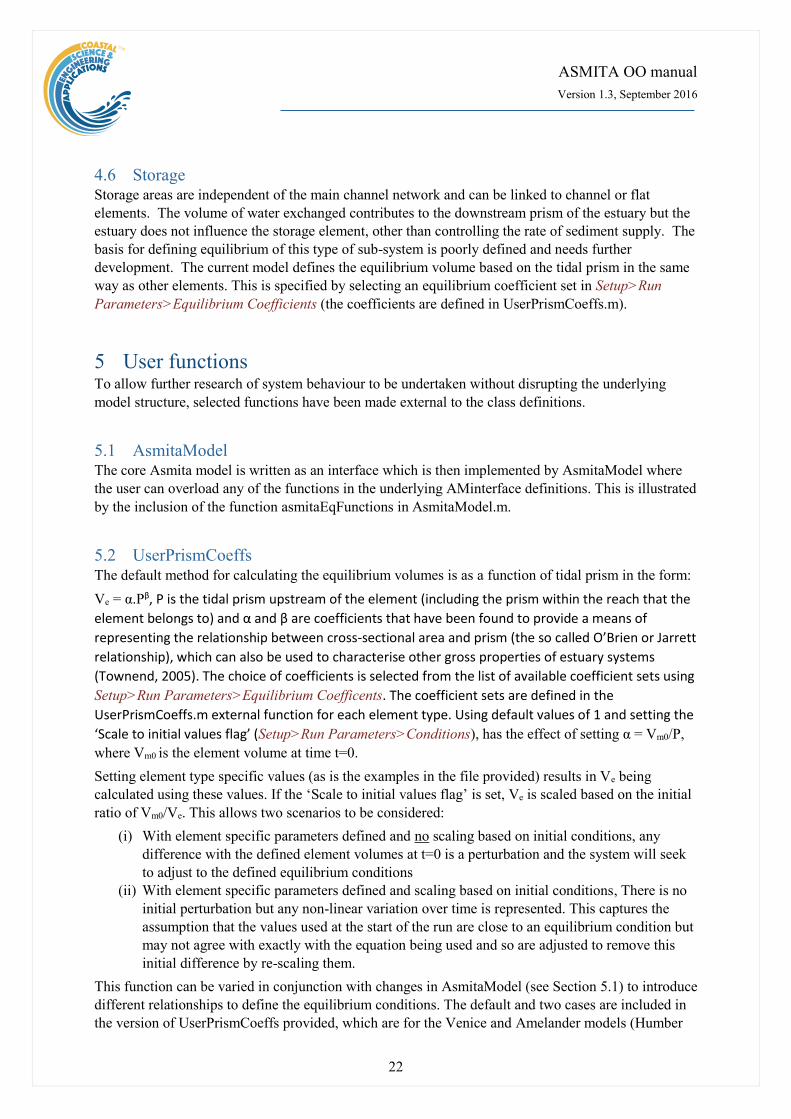
4.6 Storage Storage areas are independent of the main channel network and can be linked to channel or flat

elements. The volume of water exchanged contributes to the downstream prism of the estuary but the

estuary does not influence the storage element, other than controlling the rate of sediment supply. The

basis for defining equilibrium of this type of sub-system is poorly defined and needs further

development. The current model defines the equilibrium volume based on the tidal prism in the same

way as other elements. This is specified by selecting an equilibrium coefficient set in Setup>Run

Parameters>Equilibrium Coefficients (the coefficients are defined in UserPrismCoeffs.m).

5 User functions To allow further research of system behaviour to be undertaken without disrupting the underlying

model structure, selected functions have been made external to the class definitions.

5.1 AsmitaModel The core Asmita model is written as an interface which is then implemented by AsmitaModel where

the user can overload any of the functions in the underlying AMinterface definitions. This is illustrated

by the inclusion of the function asmitaEqFunctions in AsmitaModel.m.

5.2 UserPrismCoeffs The default method for calculating the equilibrium volumes is as a function of tidal prism in the form:

Ve = α.Pβ, P is the tidal prism upstream of the element (including the prism within the reach that the

element belongs to) and α and β are coefficients that have been found to provide a means of

representing the relationship between cross-sectional area and prism (the so called O’Brien or Jarrett

relationship), which can also be used to characterise other gross properties of estuary systems

(Townend, 2005). The choice of coefficients is selected from the list of available coefficient sets using

Setup>Run Parameters>Equilibrium Coefficents. The coefficient sets are defined in the

UserPrismCoeffs.m external function for each element type. Using default values of 1 and setting the

‘Scale to initial values flag’ (Setup>Run Parameters>Conditions), has the effect of setting α = Vm0/P,

where Vm0 is the element volume at time t=0.

Setting element type specific values (as is the examples in the file provided) results in Ve being

calculated using these values. If the ‘Scale to initial values flag’ is set, Ve is scaled based on the initial

ratio of Vm0/Ve. This allows two scenarios to be considered:

(i) With element specific parameters defined and no scaling based on initial conditions, any

difference with the defined element volumes at t=0 is a perturbation and the system will seek

to adjust to the defined equilibrium conditions

(ii) With element specific parameters defined and scaling based on initial conditions, There is no

initial perturbation but any non-linear variation over time is represented. This captures the

assumption that the values used at the start of the run are close to an equilibrium condition but

may not agree with exactly with the equation being used and so are adjusted to remove this

initial difference by re-scaling them.

This function can be varied in conjunction with changes in AsmitaModel (see Section 5.1) to introduce

different relationships to define the equilibrium conditions. The default and two cases are included in

the version of UserPrismCoeffs provided, which are for the Venice and Amelander models (Humber

ASMITA OO manual


23

uses the default settings in the example file provided). Note that in the Amelander model a constant

value is assigned to tidalflat equilibrium by setting alpha to this value and beta to zero.

5.3 UserSLRrate The rate of sea level rise is defined in Setup>Estuary> Water Levels and can be positive or negative.

The amount of sea level rise at time, t, is computed in UserSLRrate.m.

By defining a rate < -9 m/year, an alternative calculation is applied. In the example file this is a linear

rise of 1mm/year prior to 1900 and an exponential rate of increase thereafter that approximates IPCC

projections used in the UK (circa 2010). [Note: for this to work the Start Year (set in Setup>Run

Parameters>Time Step) must be prior to 1900.] However, this function can be replaced by any

function that returns the amount of sea level rise at model run time from t=0.

5.4 UserUnitTesting This function is for developers to test differences against existing cases when the code is modified. It

makes use of the class AsmitaTest and currently can run with one of three models: Humber 3EM.mat,

Venice 9EM.mat Severn 16EM.mat. The model setup files are supplied as read only and if unmodified

are compatible with the results files provided. These are named HumberTestData.mat,

VeniceTestData.mat, SevernTestData.mat(also all read only). To run a particular case simply run

UserUnitTesting from the command prompt and select a case from the list dialog box. All prompts

from Asmita OO are suppressed when run via this utility.

6 Program Structure The overall structure of the code is illustrated schematically in Figure 17. This is implemented through

a number of classes that handle the graphical user interface and program workflows and a number of

classes that represent parts of the system. The former comprises the following classes:

Figure 17 – High level schematic of program

structure

GUIinterface – basic functionality of model GUI

Asmita – implements GUIinterface for ASMITA

application

DataGUIinterface – basic functionality for Data selection

AsmitaPlots – implements DATAGUIinterface to plot

results

Project – details of setup and model runs (scenarios)

ConstantData – defines constants used in model

RunProps – defines run time properties (eg time step)

RunModel – handles the initialisation, running and posting

of model results

AMinterface – basic functionality of the Asmita model

AsmitaModel – implements AMinterface allowing

specific applications to overload function in the basic

implementation provided in the interface

Results – store model run results as scenarios and handle

saving scenarios to an excel file

ASMITA OO manual


24

The classes to define the inlet or estuary system, currently include the following:

Estuary – properties and methods for system as a whole such as dispersion and linkages

Reach – setup and provide access to properties for reaches (a channel element plus linked elements)

Element – setup and provide access to element properties

Advection – handles all types of advective flow, including rivers, drift and tidal pumping

Rivers – setup and provide access to river flow/sediment inputs

Drift – setup and provide access to littoral drift sediment inputs

Interventions – setup and provide access to imposed changes to system geometry (volume and area)

WaterLevels – setup and access to water level definitions, tidal properties and changes over time

Saltmarsh – setup and access to saltmarsh properties and functions to define behaviour

Hydraulics – not yet implemented.

The order in which functions are called during initialisation and runtime is important because of the

interdependence of parameters across the various classes. The call sequence is detailed in Appendix A

– Function call sequence in RunModel and the UML class diagrams are included in Appendix B –

UML Class diagrams.

7 Additional References Gray, A.J., 1992. Saltmarsh plant ecology: zonation and succession revisited. In: J.R.L. Allen, K. Pye

(Eds.), Saltmarshes: Morphodynamics, conservation and engineering significance. Cambridge

University Press, Cambridge, pp. 63-79.

Randerson, P.F., 1979. A simulation of saltmarsh development and plant ecology. In: B. Knights, A.J.

Phillips (Eds.), Estuarine and coastal land reclamation and water storage. Saxon House,

Farnborough, pp. 48-67.

Silvestri, S., Defina, A., Marani, M., 2005. Tidal regime, salinity and salt marsh plant zonation.

Estuarine, Coastal and Shelf Science, 62, 119-130.

Townend, I.H., 2005. An examination of empirical stability relationships for UK estuaries. Journal of

Coastal Research, 21(5), 1042-1053.

Townend, I.H., Rossington, S.K., Knaapen, M.A.F., Richardson, S., 2010. The dynamics of intertidal

mudflat and saltmarshes within estuaries. In: J. Mckee Smith (Ed.). Proceedings of the

International Conference on Coastal Engineering. Coastal Engineering Research Council, pp.

1-10.

Townend, I.H., Wang, Z.B., Rees, J.G., 2007. Millennial to annual volume changes in the Humber

Estuary. Proc.R.Soc.A, 463, 837-854.

Townend, I.H., Wang, Z.B., Stive, M.J.E., Zhou, Z., 2016a. Development and extension of an

aggregated scale model: Part 1 – Background to ASMITA. China Ocean Engineering, 30(4),

482-504.

Townend, I.H., Wang, Z.B., Stive, M.J.E., Zhou, Z., 2016b. Development and extension of an

aggregated scale model: Part 2 – Extensions to ASMITA. China Ocean Engineering, 30(5),

651-670.

van Goor, M.A., Zitman, T.J., Wang, Z.B., Stive, M.J.F., 2003. Impact of sea-level rise on the

morphological equilibrium state of tidal inlets. Marine Geology, 202, 211-227.

Wang, Z.B., de Vriend, H.J., Stive, M.J.F., Townend, I.H., 2007. On the parameter setting of semi-

empirical long-term morphological models for estuaries and tidal lagoons. In: C.M. Dohmen-

Janssen, S.J.M.H. Hulscher (Eds.). River, Coastal and Estuarine Morphodynamics. Taylor &

Francis, pp. 103-111.

ASMITA OO manual


25

Wang, Z.B., de Vriend, H.J., Stive, M.J.F., Townend, I.H., 2008. On the parameter setting of semi-

empirical long-term morphological models for estuaries and tidal lagoons. In: C.M. Dohmen-

Janssen, S.J.M.H. Hulscher (Eds.). River, Coastal and Estuarine Morphodynamics. Taylor &

Francis, pp. 103-111.

Wang, Z.B., Townend, I.H., Stive, M.J.E., 2014. Modelling of morphological response of tidal basins

to sea-level rise revisited, Proceedings of the 17th Physics of Estuaries and Coastal Seas

(PECS) conference, Porto de Galinhas, Pernambuco, Brazil.

ASMITA OO manual


26

Appendix A – Function call sequence in RunModel

The following table provides a listing of the calls made in RunModel and the dependency of the

functions called on other (sub) functions, along with a summary of the input and output parameters

using the model notation (see individual functions or class property definitions for full explanation of

variables).

ASMITA OO manual


27

ID Calls in RunModel.Run First Sub-function calls Further Sub-function calls Inputs Outputs Depends on

From initial model setup 0

A RunModel.CheckInput

B Project.Scenario

C

RunModel.InitialiseModel

1 Results.clearRunResults Cases.Year,RunData,EleData set to [] 0

2 AsmitaModel.setAsmitaModel calls getAsmitaModel and instantiates

AsmitaModel; initialises eqScaling=1

0

RunModel.initialiseModelParameters - this is also used to initialise various gui functions (eg Response)

3 Element.intialiseElements initial volumes and areas transient values of vm, sm, vf, sf and ws at

t=0 and transEleType

0

4 Element.setEqConcentration transEleType and Eq. Conc. assign cE to elements (allows for mixed

fractions)

0

5 WaterLevels.newWaterLevels water level properties at t=0 transient water level properties at t=0 0

6 Element.setEleWLchange dHWchange,dLWchange, EleType assign WL change based on element type 0, 6

7 Estuary.intialiseReachGraph D, dExt ReachGraph to define connectivity and

dispersion

0

8 Advection.initialiseRiverGraph

Advection.initialiseDriftGraph

Q, qIn, qOut flow graph for each type of advection 0

10 Reach.setReach (reachEleID) assign reach id to elements (for plotting) 0

11 Reach.setReachProps Moving volume and area, WLs HW/LW volume, area, prism, csa, uriv, 3,5

12 Advection.setTidalPumping RiverGraph, (qtp, qtpIn, qtpOut)

13 Advection.getTidalPumpingDischargeh, ws'', xi, avCSA, uriv, +props qtp, qtp0 for each reach 3,5,11

14 Interventions.getInterventions user defined changes in area and

volume for any given year

Unique years and array of change for each

element (dV and dS)

0

15 Saltmarsh.concOverMarsh EleType,cE,ws,S2,M2,zhw,zlw, MarshDepthConc 0

16 Saltmarsh.singleBioSettlingRate dmx,bmx,wsa,wsb,Bc,

(depth,aws1,aws2)

ws' 0

17 Saltmarsh.BiomassCoeffs dmn, dmx, bmx Bc 0

18 AsmitaModel.asmitaEqFunctions alpha, beta, EleType, Prism EqVolume, ve 3,11

19 Saltmarsh.EqDepths dmn,dmx,dslr,tr,cE,sm,vm,(ws') Deq' 3,6

20 Saltmarsh.BioSettlingRate ws, sm,vm,ve,bmx,wsa,wsb,(Bm) ws' 3

21 Saltmarsh.Biomass vm, sm, (Bc) Bm 3

22 Saltmarsh.Morris kbm, qm, dslr, (Bc) Deq 0

23 Saltmarsh.BiomassCoeffs dmn, dmx, bmx Bc 0

9 AsmitaModel.setDQmatrix cE, kCeI DQ and dqIn 7,8,12

45 Advection.getAdvection Flow uses advection graphs Q, qIn and qOut for each type of advection

24 AsmitaModel.setVertExch vm,vf,Vo,ve,cb,n,(ws'),(B),(dd) ws'' 9,19,40+41(using7&8)

20 Saltmarsh.BioSettlingRate ws, sm,vm,ve,bmx,wsa,wsb,(Bm) ws' 3

25 Element.setEleAdvOffsets Offset flags, n, B and dd eqCorV offset correction 40+41(using 7&8)

26 AsmitaModel.asmitaEqScalingCoeffs initial volumes, (EqVolume) eqScaling coefficient 3

18 AsmitaModel.asmitaEqFunctions alpha, beta, EleType, Prism EqVolume based on initial prism 3,11

19 Saltmarsh.EqDepths+subfunctions dmn,dmx,dslr,tr,cE,sm,vm,(ws') Deq' 3,6

27 Element.setEquilibrium eqScaling, eqAdvOffSet EqVolume, ve, corrected for any scaling 2, 12

18 AsmitaModel.asmitaEqFunctions alpha, beta, EleType, Prism EqVolume, ve 3,11

19 Saltmarsh.EqDepths+subfunctions dmn,dmx,dslr,tr,cE,sm,vm,(ws') Deq' 3,6

28 Element.setEleConcentration assign concentrations, conc, to elements 0

29 AsmitaModel.asmitaConcentrations vm, ve, sm, ws'', n, D, dExt, Q, cE,

qIn, kCeI

array of concentrations, conc 3,18,24

30 RunModel.CheckStability vm, D , Q, cnc, NumSteps,

TimeStep, outInt

Runsteps, delta, outInt 0, 5, 15

31 RunModel.PostTimeStep outInt

32 Results.setResults WLs and vm, vf, ve, cnc, dWL intialise Results if not already instantiated,

populate Year, RunData, EleData

3,6,11,18

RunModel.InitTimeStep

jt, delta, Time, DateTime iStep, Time, DateTime main

5 WaterLevels.newWaterLevels water level properties at t=t(i) transient water level properties at t=t(i) -

6 Element.setEleWLchange dHWchange,dLWchange, EleType assign WL change based on element type -

33 Interventions.setAnnualChange Year,dV,dS, vm,vf,sm,sf vm,vf,sm,sf -

34 Estuary.updateReachGraph for dynamic elements - not yet implemented

35 function to make adjustments

41 Advection.updateAdvectionGraphs for dynamic elements - not yet implemented

36 function to make adjustments

11 Reach.setReachProps Moving volume and area, WLs HW/LW volume, area and prism at t=t(i) 5,33,34,8

12 Advection.setTidalPumping RiverGraph, (qtp, qtpIn, qtpOut) 8

13 Advection.getTidalPumpingDischargeh, ws'', xi, avCSA, uriv, +props qtp, qtp0 for each reach 11+E-1

27 Element.setEquilibrium eqScaling, eqAdvOffSet EqVolume, ve, corrected for any scaling 11+E-1

18 AsmitaModel.asmitaEqFunctions alpha, beta, EleType, Prism EqVolume, ve 11+E-1

19 Saltmarsh.EqDepths+subfunctions dmn,dmx,dslr,tr,cE,sm,vm,(ws') 6+E-1

37 Element.setEqConcentration Not implemented: only needed if cE is varied during run

9 AsmitaModel.setDQmatrix cE, kCeI DQ and dqIn 34,41

45 Advection.getAdvection Flow uses advection graphs Q, qIn and qOut for each type of advection

24 AsmitaModel.setVertExch vm,vf,Vo,ve,cb,n,(ws'),(B),(dd) ws'' 9,E-1,40+41(using E-1)

20 Saltmarsh.BioSettlingRate ws, sm,vm,ve,bmx,wsa,wsb,(Bm) ws' E-1

RunModel.RunTimeStep

38 AsmitaModel.asmitaVolumeChange dwl, vm, vf, ve, sm, n , cb assign transient values of vm,vf,vb,conc to

elements

6,E-1

29 AsmitaModel.asmitaConcentrations vm, ve, sm, ws'', n, D, dExt, Q, cE,

qIn, kCeI

conc E-1,24

39 Saltmarsh.BioProduction kbm,(Bm)

21 Saltmarsh.Biomass vm, sm, (Bc) Bm E-1

23 Saltmarsh.BiomassCoeffs dmn, dmx, bmx Bc

40 AsmitaModel.BddMatrices sm,ws'',n,Q,cE,(DQ,dqIn) B and dd E-1

42 AsmitaModel.MassBalance delta, Time, dExt, cE, cb, cI, cnc, qIn,

qOut, Vo, vf, vm, vb, shw, dwl

dWLVolume, SedMbal, WatMbal E

RunModel.PostTimeStep

iStep, outInt D

32 Results.setResults WLs and vm, vf, ve, cnc, dWL intialise Results if not already instantiated,

populate Year, RunData, EleData

E

RunModel.PostResults

sedMbal, WatMbal message to user 42

43 Results.saveResults Year, RunData, EleData CaseData, CaseResults 32

ASMITA OO manual


28

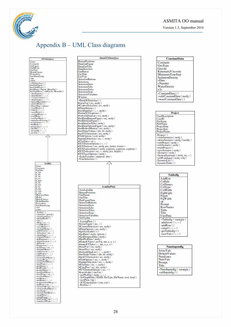
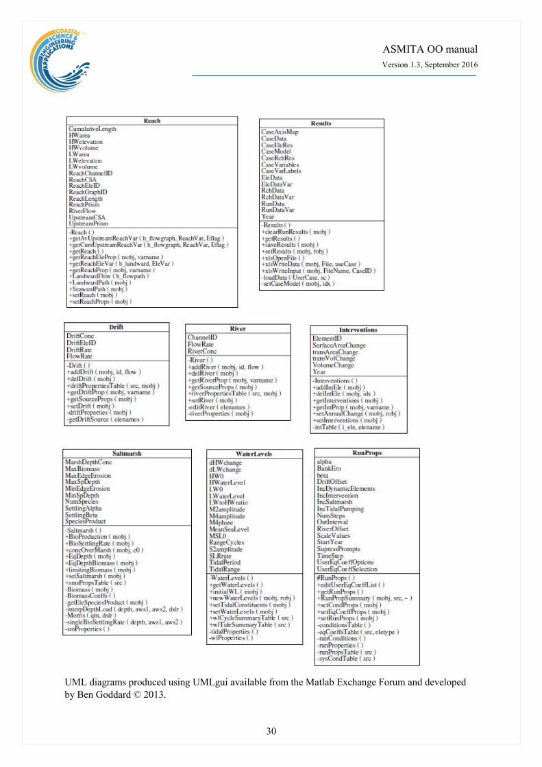
Appendix B – UML Class diagrams

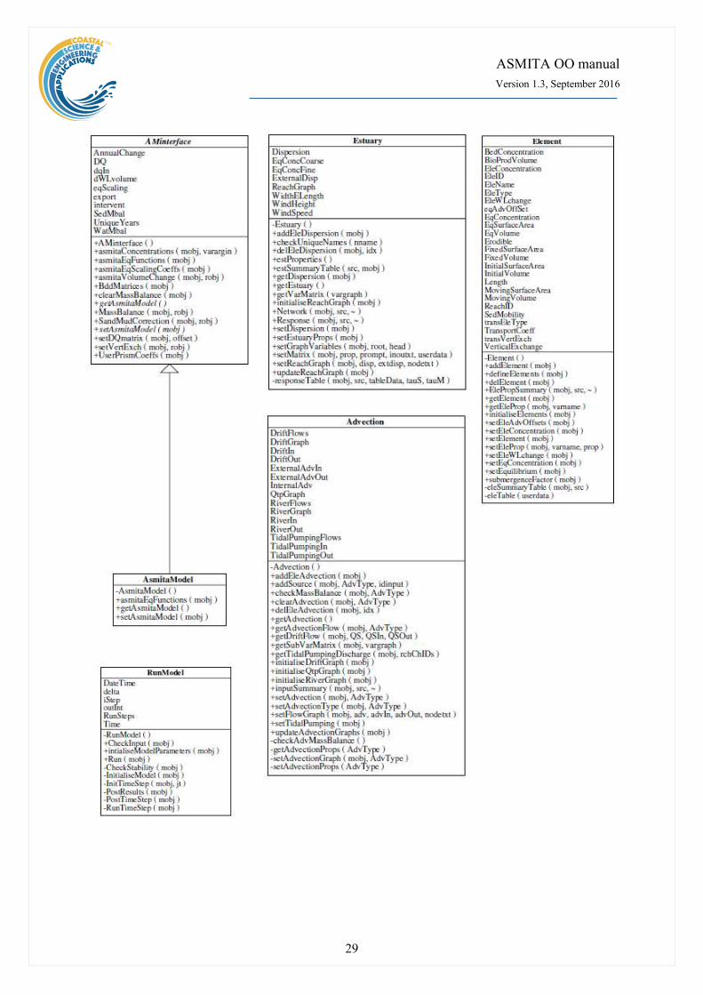
ASMITA OO manual


29

ASMITA OO manual


30

UML diagrams produced using UMLgui available from the Matlab Exchange Forum and developed

by Ben Goddard © 2013.

Documents

Requirements Resources Bibliography - coastalsea.uk€¦ · 2.1 ASMITA OO software ... 2.3 Typical workflow to set-up new model ... concepts and methodology used in long-term morphological