Embed Size (px)
Citation preview

REPUBLIC OF BOTSWANA
Department of Crop Production (DCP) Ministry of Agriculture
CONSULTANCY SERVICES FOR THE FEASIBILITY STUDY FOR THE ZAMBEZI
INTEGRATED AGRO-COMMERCIAL DEVELOPMENT PROJECT
CONCEPTUAL DESIGN REPORT – FINAL REPORT
REVISION
DESCRIPTION DATE YY mm DD BY APPROVED NOTES
FINAL VERSION 2014 December 19 CP/FA AG
AMENDED VERSION
(after comments) 2015 March 31 CP/FA AG
SGI Studio Galli Ingegneria S.p.A
in Joint Venture with
Metaferia Consulting Engineers PLC
MCE

Zambezi Integrated Agro-Commercial Development Project
SGI & MCE page i Final Report Rev. 01
TABLE OF CONTENTS
TABLE OF CONTENTS ....................................................................................................................... I
LIST OF ACRONYMS AND ABBREVIATIONS ........................................................................... XI
0 SUMMARY ................................................................................................................................... 13
1 INTRODUCTION ........................................................................................................................ 14
1.1 General issues ....................................................................................................................... 14
1.2 Land use and land cover ........................................................................................................ 14
1.3 Climate .................................................................................................................................. 15
1.4 Current state of irrigation ...................................................................................................... 15
1.5 Objectives of the study .......................................................................................................... 15
2 CLIMATE AND HYDROLOGY ................................................................................................ 16
2.1 General framework ............................................................................................................... 16
2.2 Data sources and type ........................................................................................................... 16
2.3 Data assessment for agronomic study ................................................................................... 16
2.4 Statistical analysis of rainfall ................................................................................................ 22
3 HYDROGEOLOGY ..................................................................................................................... 28
3.1 General hydrogeological framework..................................................................................... 28
3.2 Data gathering and previous study ........................................................................................ 30
3.3 Planning of field survey ........................................................................................................ 35
4 ONFARM IRRIGATION SYSTEM DESIGN ........................................................................... 38
4.1 Planning of irrigation system ................................................................................................ 38
4.1.1 Design criteria .......................................................................................................... 38
4.1.2 Land resource ........................................................................................................... 38
4.1.3 Water resource .......................................................................................................... 39
4.2 Options identification and assessment .................................................................................. 40
4.2.1 Alternatives of different pressurized irrigation system ............................................ 41
4.2.2 Selection of continuous over conventional sprinkler system ................................... 43
4.2.3 Centre pivot irrigation system .................................................................................. 43
4.2.4 Centre pivot with corner attachment and/or end guns .............................................. 45
4.2.5 Linear move sprinkler .............................................................................................. 45
4.2.6 Side role sprinkler .................................................................................................... 46
4.2.7 Big gun sprinkler ...................................................................................................... 47
4.2.8 Drip irrigation system ............................................................................................... 47
Zambezi Integrated Agro-Commercial Development Project
SGI & MCE page ii Final Report Rev. 01
4.2.9 Final selection of irrigation system .......................................................................... 48
4.3 Crop water requirements ....................................................................................................... 49
4.3.1 Reference crop evapotranspiration ........................................................................... 49
4.3.2 Effective rainfall ....................................................................................................... 50
4.3.3 Cropping pattern ....................................................................................................... 50
4.3.4 Net irrigation requirements...................................................................................... 51
4.3.5 Irrigation efficiency .................................................................................................. 51
4.3.6 Gross irrigation requirements .................................................................................. 52
4.3.7 Irrigation duty .......................................................................................................... 52
4.4 Sprinkler irrigation system design ........................................................................................ 53
4.4.1 Gross application depth ............................................................................................ 53
4.4.2 System capacity ........................................................................................................ 54
4.4.3 Irrigation scheduling ................................................................................................. 54
4.5 Drip irrigation system design ................................................................................................ 56
4.5.1 Water requirement for fruit trees .............................................................................. 56
4.5.2 General layout of fruit field ...................................................................................... 57
4.5.3 Basic design units (BDU) of a cluster ...................................................................... 58
4.5.4 Selection of drippers, type, spacing and discharge ................................................... 60
4.5.5 Design of laterals ...................................................................................................... 61
4.5.6 Design of manifolds ................................................................................................. 63
4.6 Maintenance of irrigation systems ........................................................................................ 64
4.6.1 Sprinkler ................................................................................................................... 65
4.6.2 Drip ........................................................................................................................... 66
4.6.3 Filters ........................................................................................................................ 66
4.6.4 Chemical Control Measures ..................................................................................... 67
4.6.5 Bacterial Slimes/Precipitates .................................................................................... 67
4.6.6 Algae and Aquatic Plants ......................................................................................... 68
4.6.7 Chemical Precipitation of Iron ................................................................................. 68
4.6.8 Chlorine precipitation ............................................................................................... 68
4.6.9 pH Control ................................................................................................................ 68
4.6.10 Iron Sulfide Precipitation ......................................................................................... 68
4.6.11 Precipitation of Calcium Salts .................................................................................. 69
4.7 References for irrigation system design ................................................................................ 70
5 ON DEMAND PRESSURIZED PIPED IRRIGATION SYSTEM .......................................... 71
5.1 Introduction ........................................................................................................................... 71
5.2 Identification of pipelines layout .......................................................................................... 72

Zambezi Integrated Agro-Commercial Development Project
SGI & MCE page iii Final Report Rev. 01
5.3 Design of pipeline network ................................................................................................... 75
5.3.1 General aspects and hydraulic criteria ...................................................................... 75
5.3.2 Pipe materials ........................................................................................................... 76
5.4 Implementation of COPAM model for hydraulic simulation ............................................... 78
5.4.1 Theoretical background ............................................................................................ 80
5.4.2 Geometry and input .................................................................................................. 81
5.4.3 Simulation results ..................................................................................................... 82
5.4.4 Pumping system and power requirements ................................................................ 86
6 DRAINAGE SYSTEM AND ROADS ......................................................................................... 92
6.1 Introduction ........................................................................................................................... 92
6.2 Identification of drain and road layout .................................................................................. 92
6.3 Estimation of storm water runoff .......................................................................................... 94
6.3.1 Identification of watersheds ..................................................................................... 94
6.3.2 Time of concentration .............................................................................................. 96
6.3.3 Spatial analysis of rainfall ........................................................................................ 98
6.3.4 Runoff peak and hydrograph .................................................................................. 100
6.4 Design of gravity drainage system ...................................................................................... 103
6.4.1 Design criteria ........................................................................................................ 103
6.4.2 Hydraulic dimensioning of primary and secondary drains ..................................... 105
6.5 Design of roads ................................................................................................................... 108
6.6 Storm water and sediment management ............................................................................. 111
6.6.1 Evaluation of soil losses ......................................................................................... 111
6.6.2 Sediment transport .................................................................................................. 113
6.6.3 Banks, sediment traps, detention and storm water ponds ....................................... 114
6.7 Drain maintenance .............................................................................................................. 121
7 COST ESTIMATION AND WORK PLAN ............................................................................. 122
8 FINAL CONSIDERATION ABOUT ZIACDP FEASIBILITY ............................................. 127
9 ANNEXES ................................................................................................................................... 128
9.1 Soil physical and chemical properties ................................................................................. 128
9.1.1 Soil parameters from profile pits on sandy soils .................................................... 128
9.1.2 Soil parameters from profile pits on loamy sand soils ........................................... 130
9.1.3 Soil parameters from profile pits on sandy loam soils ........................................... 130
9.1.4 Soil parameters from profile pits on sandy loam soils ........................................... 131
9.2 Calculation related to crop water requirement .................................................................... 132
9.2.1 Details of crop water requirement for sorghum as a supplementary irrigation ...... 132

Zambezi Integrated Agro-Commercial Development Project
SGI & MCE page iv Final Report Rev. 01
9.2.2 Details of crop water requirement for sunflower as a supplementary irrigation .... 133
9.2.3 Details of crop water requirement for beans as a supplementary irrigation ........... 133
9.2.4 Details of crop water requirement for maize as a supplementary irrigation ........... 134
9.2.5 Details of crop water requirement for wheat as a full-fledged irrigation ............... 134
9.2.6 Details of crop water requirement for soybean as a full-fledged irrigation ............ 135
9.2.7 Details of crop water requirement for alfalfa as a full-fledged annual irrigation ... 135
9.2.8 Details of crop water requirement for mango as a full-fledged annual irrigation .. 136
9.3 Flow chart of continuous move sprinkler system design .................................................... 137
9.4 Design table of drip irrigation system ................................................................................. 138

Zambezi Integrated Agro-Commercial Development Project
SGI & MCE page v Final Report Rev. 01
LIST OF DRAWINGS
All. 9.1 Irrigation Layout
All. 9.2 Drainage Layout
All. 9.3 Road Layout
All. 9.4 Drain Profile (1/2)
All. 9.5 Drain Profile (2/2)
All. 9.6 Drain Design
All. 9.7 Drain cross sections
All. 9.8 Detention and storm water ponds
All. 9.9 Typical cross section of primary road
All. 9.10 Typical cross section of secondary road
All. 9.11 Typical cross section of field road
All. 9.12 Pumping station
All. 9.13 Typical village layout
All. 9.14 Typical housing layout
All. 9.15 Plan type D house
All. 9.16 Workshop plan
All. 9.17 Office plan
All. 9.18 Store

Zambezi Integrated Agro-Commercial Development Project
SGI & MCE page vi Final Report Rev. 01
LIST OF FIGURES
Figure 1. Annual Rainfall at Pandamatenga (Police Station, 1962 – 2006, DMS) ................. 17
Figure 2. Average Monthly Rainfall at Pandamatenga (Police Station, 1962 – 2006,
DMS) ..................................................................................................................... 18
Figure 3. Average Daily Rainfall at Pandamatenga (Police Station, 1962 – 2006, DMS) ...... 18
Figure 4. Temperature at Pandamatenga (Meteorological Station, 1998 – 2012, DMS) ......... 19
Figure 5. Sunshine hours at Pandamatenga (Meteorological Station, 1998 – 2011, DMS) ..... 19
Figure 6. Relative humidity at Maun (Airport Station, NWMPR / Botswana National
Atlas) ..................................................................................................................... 20
Figure 7. Wind speed at Kasane (Airport Station, NWMPR and estimation) ......................... 21
Figure 8. Pan evaporation at Pandamatenga (Meteorological Station, 1997 – 2012,
DMS) ..................................................................................................................... 21
Figure 9. Maximum Daily Rainfall at Pandamatenga (Police Station, 1962 – 2006, DMS) ... 23
Figure 10 Intensity–duration–frequency relationship for storm event with duration more
than one hour ......................................................................................................... 26
Figure 11 Intensity–duration–frequency relationship for storm event with duration less
than one hour ......................................................................................................... 27
Figure 12. Map of Average depth of Groundwater (Department of Surveys and
Mapping, 2001) ..................................................................................................... 29
Figure 13. Map of Mean Annual Recharge (Doll and Fiedler, 2008) ..................................... 30
Figure 14. Layout of previous local geotechnical investigations (Consultant’s
elaboration, 2014) .................................................................................................. 31
Figure 15. Map of Hydrogeological Survey results (Consultant’s elaboration, 2014) ........... 33
Figure 16. Layout of realized borehole for hydrogeological survey (Consultant’s
elaboration, 2014) .................................................................................................. 36
Figure 17. Map of Absolute Water Level and Flow Direction (Consultant’s elaboration,
2014) 37
Figure 18 Schematic functioning of hand move sprinkler system ........................................... 42
Figure 19 Example of continuous type sprinkler irrigation system ......................................... 43
Figure 20 Example of alignment of center pivot ..................................................................... 44
Figure 21 Center pivot sprinkler working in the field ............................................................. 44
Figure 22 Example of center pivot with corner attachment ..................................................... 45
Figure 23 Linear move supplied to the linear move through a canal ....................................... 46
Figure 24 Side roll sprinkler system ........................................................................................ 46
Figure 25 Big gun sprinkler system ......................................................................................... 47
Figure 26 Layout of drip irrigation system showing the significance of reduced/wetted
area as compared to the total area ......................................................................... 48
Zambezi Integrated Agro-Commercial Development Project
SGI & MCE page vii Final Report Rev. 01
Figure 27 Typical layout of drip irrigation system .................................................................. 58
Figure 28 Basic Design Unit of a Cluster, for fruit .................................................................. 59
Figure 29 Basic Design of one plot .......................................................................................... 60
Figure 30. The already designed Chobe – Zambesi water transfer scheme (“Preliminary
Design Report on Utilization of the Water Resources of the Chobe/Zambezi
River” by WRC, 2013) .......................................................................................... 71
Figure 31. Layout of primary pipes and irrigation lots ............................................................ 72
Figure 32. Layout of secondary pipes and irrigation system (center pivot and drip) .............. 73
Figure 33. Proposed alignment of center pivots, secondary pipes and WTS ........................... 74
Figure 34. Proposed alignment of center pivots, secondary pipes and WTS (details) ............. 75
Figure 35. Key steps of an irrigation system development scheme (FAO, 2000) ................... 79
Figure 36. Synthetic flow chart of COPAM software (FAO, 2000) ........................................ 80
Figure 37. Supplied discharge along primary pipes for the study area .................................... 85
Figure 38. Diameter of primary pipes for the study area ......................................................... 86
Figure 39. Piezometry along primary pipes for the study area ............................................... 89
Figure 40. General layout of drainage system and access roads for existing farms
(“Consultancy Services for Construction Supervision of Road Network and
Drainage Systems for Pandamatenga Farms – Final Design” by DIWI in
2011)...................................................................................................................... 92
Figure 41. Layout of primary drains for the present design and drainage system of the
existing farms ........................................................................................................ 93
Figure 42. Main watersheds of drainage system ...................................................................... 94
Figure 43. Layout of primary and secondary drains for the present design and drainage
system of the existing farms .................................................................................. 95
Figure 44. Schematic layout of drainage system for fields towards the secondary drains ...... 96
Figure 45 ARF related to storm duration and catchment area (Technical Report NWS 24,
NOAA) .................................................................................................................. 98
Figure 46 ARF related to rainfall intensity and catchment area (Botswana Road Design
Manual) ................................................................................................................. 99
Figure 47 Triangular shaped hydrograph related to hydrograph peak reduction factor
included in Table 35 (Wanielista, Yousef “Stormwater Management”, 1993) ... 100
Figure 48 Typical cross section of drains .............................................................................. 106
Figure 48 Layout of primary drains and their code ............................................................... 106
Figure 49 Layout of roads ...................................................................................................... 109
Figure 50 Typical cross section of primary road ................................................................... 109
Figure 51 Typical cross section of secondary road ................................................................ 110
Figure 52 Typical cross section of field road ......................................................................... 110
Figure 53 Detail about the composition of primary and secondary road ............................... 110
Figure 54 Detail about the composition of field road ............................................................ 111

Zambezi Integrated Agro-Commercial Development Project
SGI & MCE page viii Final Report Rev. 01
Figure 55 Planimetric view and cross section of fields, drain and road to identify
designed banks .................................................................................................... 115
Figure 48 Outlet scheme of storm water from fields ............................................................. 115
Figure 48 Typical cross section of drain where field outlet is located ................................... 116
Figure 48 View of the drain slope where field outlet is located ............................................ 116
Figure 55 Cross section of designed banks ............................................................................ 117
Figure 56 Schematic functioning of sediment traps ............................................................... 117
Figure 57 Positioning of sediment traps along the primary drains ........................................ 118
Figure 58 Planimetric view and longitudinal along primary drain to identify designed
sediment traps ...................................................................................................... 119
Figure 59 Planimetric view of terminal portion of a primary drain and connection with
detention and storm water ponds ......................................................................... 120

Zambezi Integrated Agro-Commercial Development Project
SGI & MCE page ix Final Report Rev. 01
LIST OF TABLES
Table 1 Summary of meteorological parameters for agronomic study .................................... 22
Table 2 Statistical elaboration of maximum daily rainfall at Pandamatenga ........................... 24
Table 3 Parameters of Gumbel analysis for maximum daily rainfall Pandamatenga .............. 24
Table 4 Daily rainfall heights related to return time of storm event at Pandamatenga ............ 25
Table 5 Daily rainfall heights related to return time of storm event at Pandamatenga
(TAHAL, 2009) ..................................................................................................... 25
Table 6 Conversion factor for daily rainfall heights (NWMPR, 2006) ................................... 25
Table 7 Rainfall heights related to return time and duration of storm event at
Pandamatenga ........................................................................................................ 26
Table 8 Stratigraphic description regarding soils in borehole DH1 ................................... 32
Table 9 Stratigraphic description regarding soils in borehole DH2 ................................... 32
Table 10 Stratigraphic description regarding soils in borehole DH3 ................................... 32
Table 11 Stratigraphic description regarding soils in borehole DH4 ................................... 32
Table 12 Depth of Static Water Level upon completion of drilling and after several
days (TAHAL Group Hydrogeological Survey, 2008) ......................................... 34
Table 13 The thickness of the various beds from surface downward (TAHAL Group
Hydrogeological Survey, 2008) ............................................................................ 35
Table 14 Available values of Static Water Level and Absolute Water Level ...................... 36
Table 15 Classified area as per the textural analysis ............................................................... 39
Table 16 Average values of soil physical properties of the study area .................................... 39
Table 17 Input climate data to determine ETo using Penman method of FAO
CROPWAT computer model ................................................................................ 50
Table 18 Cropping patterns for wet and dry season ................................................................. 51
Table 19 Summary of design criteria used for design of centre pivot sprinkler package ........ 55
Table 20 Specifications of centre pivot sprinkler package ...................................................... 56
Table 21 Design parameters of drip irrigation ......................................................................... 58
Table 22 Factor F for multiple outlets ..................................................................................... 62
Table 23 Drip induction and possible problems ...................................................................... 69
Table 24 Comparison among materials for pressured water supply networks ....................... 77
Table 25 Hydraulic characteristic of pipe in relation with the number of fields that are
supplied ................................................................................................................. 83
Table 26 Geometrical and hydraulic characteristics of primary pipes supplying North
irrigation lot ........................................................................................................... 83
Table 27 Geometrical and hydraulic characteristics of primary pipes supplying Central
irrigation lot ........................................................................................................... 84
Table 28 Geometrical and hydraulic characteristics of primary pipes supplying South
irrigation lot ........................................................................................................... 85

Zambezi Integrated Agro-Commercial Development Project
SGI & MCE page x Final Report Rev. 01
Table 29 Head loss and piezometry for primary pipes supplying North irrigation lot ............ 87
Table 30 Head loss and piezometry for primary pipes supplying Central irrigation lot .......... 87
Table 31 Head loss and piezometry for primary pipes supplying South irrigation lot ............ 88
Table 32 Main characteristics of the 3 pumping system for the irrigation lots ........................ 89
Table 32 Plan of pumping system ............................................................................................ 90
Table 32 Cross section of pumping system ............................................................................. 91
Table 33 Time of concentration for watersheds drained by secondary channels .................... 97
Table 34 Time of concentration for watersheds drained by primary channels ....................... 98
Table 35 Hydrograph attenuation factor (Wanielista, Yousef “Stormwater Management”,
1993).................................................................................................................... 100
Table 36 Run-off coefficients for use in rational and modified rational methods
(“Hydrological and Hydraulic Guidelines, New Zeland”, 2012) ........................ 101
Table 37 Runoff hydrograph with 10 years return time for watersheds drained by
secondary drains .................................................................................................. 102
Table 38 Runoff hydrograph with 10 years return time for watersheds drained by
primary drains ..................................................................................................... 102
Table 39 Time return and minimum freeboard for bridge and culvert according to road
type (“Hydrological and Hydraulic Guidelines, New Zeland”, 2012) ................ 104
Table 40 Hydraulic dimensioning of secondary drains.......................................................... 107
Table 41 Cumulated discharges along the primary drains ..................................................... 107
Table 42 Hydraulic dimensioning of primary drains ............................................................. 108
Table 43 Values for parameter K to apply RUSLE method (US EPA, 1973) ...................... 112
Table 44 and Table 45 Values for parameter C and P to apply RUSLE method (US
EPA, 1973) .......................................................................................................... 112
Table 46 Sediment transport along secondary drains ............................................................ 113
Table 47 Sediment transport along primary drains ................................................................ 114
Table 48 Estimation of sediment deposition within the sediment traps ................................ 119
Table 49 Dimensioning or detention ponds ........................................................................... 120

Zambezi Integrated Agro-Commercial Development Project
SGI & MCE page xi Final Report Rev. 01
LIST OF ACRONYMS AND ABBREVIATIONS
ARF Areal Reduction Factor
a.s.l. above sea level
avg average
Consultant Consortium between SGI and MCE
COPAM Combined Optimization and Performance Analysis Model
CWR Crop Water Requirements
DEA Department of Environmental Affairs
DI Ductile iron
DMS Department of Meteorological Services
DEM Digital Elevation Model
dS/m deci-Siemens per meter
EC Electrical conductivity
ETo reference evapotranspiration
FAO Food and Agriculture Organization
GRP Glassfibre Reinforced Plastic
ha Hectare
HC Hydraulic conductivity
IDF Intensity–Duration–Frequency
IR Irrigation Requirements
m.a.s.l Meters above sea level
MCE Metaferia Consulting Engineers
MOA Ministry of Agriculture
NWMPR National Water Master Plan Review
NOAA National Oceanic and Atmospheric Administration
pH Hydrogen potential (measurement of solution acid or alkaline level)
POC Point of Connection
PVC Polyvinyl chloride
RUSLE Revised Universal Soil Loss Equation

Zambezi Integrated Agro-Commercial Development Project
SGI & MCE page xii Final Report Rev. 01
SFRM Several Flow Regimes Models
SGI Studio Galli Ingegneria SpA
Tc time of concentration
Tr Time Return
USLE Universal Soil Loss Equation
WTS Water Transfer Scheme
ZIACDP Zambezi Integrated Agro-Commercial Development Project

Zambezi Integrated Agro-Commercial Development Project
SGI & MCE page 13
Final Report Rev. 01
0 SUMMARY
This Conceptual Model Report is part of the feasibility study of the Zambezi Integrated Agro-
Commercial Development Project (ZIACDP) and has been prepared by the Consultant, Studio
Galli Ingegneria S.p.A. (SGI) and Metaferia Consulting Engineers PLC (MCE) after the
contract’s signature with the Ministry of Agriculture (MoA) of Botswana, in January 2014.
The inception phase has been completed by the middle of March carrying out desk
documentation review, kick-off meeting, field visit, data gathering and harmonization, then
planning of survey activities and deliverables.
By the 10th of July, the Field Investigation Report has been delivered with results of
topographical, geotechnical and soil survey. The current project phase envisages the redaction
of the present Conceptual Model Report but also of Agricultural Commercial Business Plan,
Financial model, ESIA and EMP. Next deliverables will be the Final Report and Bank
able Feasibility Study.
For what concerns the present project (general issues are given in paragraph 1), on the basis of
climate regime (paragraph 2), hydrogeology (paragraph 3), soil survey and land suitability
maps (see Field Investigation Report) and taking into account market and value added
opportunities, the agronomist has identified suitable crops for irrigated production and the
production technology required (see Agricultural Commercial Business Plan).
The type of irrigation system is determined according to both irrigation and hydraulic issues
(paragraph 4). Once the best alternative has been selected, the conceptual design for the water
distribution and irrigation system has been prepared (paragraph 5): this network is on demand
pressurized pipelines. Finally the project for access roads and storm water drainage system has
been carried out (paragraph 6).

Zambezi Integrated Agro-Commercial Development Project
SGI & MCE page 14
Final Report Rev. 01
1 INTRODUCTION
1.1 GENERAL ISSUES
An irrigation system is designed to use the available water as efficiently as possible by
minimizing the losses in conveyance, distribution and application. The irrigation system
consists of the following two sub-systems:
Agricultural sub-system comprising the cultivated fields with different types of crops,
farming system, and agricultural practices including the application of irrigation water
and land husbandry.
Engineering sub-system comprising various structures for storage and diversion of
water and pipe networks for water conveyance and distribution.
The ZIACD project has been identified to provide irrigation infrastructure to farmers and
entrepreneurs in a large area near the existing Pandamatenga Commercial Farms. To achieve
the above objective, the Ministry of Agriculture (MoA) that is in charge of the Project, intends
to divert water from the Chobe/Zambezi River for irrigation as well as for domestic use.
The selected area of about 45,000ha is located on the western part of the existing
Pandamatenga Commercial Farms at about 110 km South of Kazungulu, in the Northeast of
the country.
In line with the aim of improving the country’s food security and livelihood of the rural
population, diversify agriculture, contribution to the country’s GDP and creation of
employment opportunity through the strategy of development of irrigated agriculture, MoA
has initiated the development of large-scale irrigation through the investigation and
development of surface water potential of the country. Accordingly, ZIACD Irrigation Project
has been planned for implementation using high technology of pressurised irrigation system.
The present Feasibility Study focused on data collection, analysis and preliminary design. The
conceptual design of the project is finalized based on the outputs of the feasibility study. The
feasibility and conceptual design reports address different sectoral components required for
the scheme development and include climate and hydrology, topography, soils, agronomy,
livestock, socio-economy, agricultural marketing, value chain, hydraulics and irrigation
engineering and economic and financial analysis.
1.2 LAND USE AND LAND COVER
With the exception of the forest and wild life reserve areas, there are no defined land use
activities in the project area. However, adjacent to the project area, there is an established
commercial farms, Pandamatenga Commercial Farms, that grow sorghum, beans, sunflower
and other crops during the rainy period of October/November to February/March. The total
area of these farms is about 25,000 ha.
The project area is predominately characterized by bushy/shrub grassland covers but the
intensity varies from place to place. In areas where mopane (Coloophosepermum mopane)
with scattered big trees like mukuse and moshweshew exist, the area can be described as
dense shrub land.
Mukuse and moshweshew are trees with evergreen characteristic that never dry as other
vegetations do. Mopane is one of the most typical tree and shrub species found broadly in the
project area. It often occurs in silty-sandy soils but it also grows on a large variety of soils
ranging from sandy to clayey textures.
Zambezi Integrated Agro-Commercial Development Project
SGI & MCE page 15
Final Report Rev. 01
1.3 CLIMATE
The climate in the project area is semi-arid characterized by summer rainfalls. Maximum
temperatures range between 26°C and 34oC and are experienced between October to July.
Minimum temperatures range between 11°C to 20°C occurring between November and July.
Rainfall is highly variable and the annual average is about 538 mm. Most of the rain falls
between October and April, with December, January and February being the peak months.
The whole year can be subdivided into four seasons including:
Dry winter season (May to August);
Rainy summer season (November to March);
Spring (September to October);
Autumn (April to May)
The soil climate of the area is characterized by aquatic moisture and isohypertermic
temperature regimes (SMSS, 1987 technical monograph No.6). An aquatic moisture regime
occurs in poorly drained parts of the lacustrine areas (Soil Mapping and Advisory Services,
Gaborone, 1990).
1.4 CURRENT STATE OF IRRIGATION
Presently, irrigation’s contribution to overall agricultural production in the country is
insignificant. Nevertheless, there is a need to expand production to feed the population and to
ensure food security. Raising livestock has long been one of the most important agricultural
activities in Botswana. Sheep and goats are said to adapt to the drought condition of the
country better than cattle do. Cattle are mostly raised for beef. Dairy and the likes are very
limited.
1.5 OBJECTIVES OF THE STUDY
As outlined in the terms of reference (ToR) for the ZIACD Project, the primary objective of
the planned intervention is to “establish a viable commercial agricultural development, which
will improve Botswana’s food security, diversify agriculture, meaningfully contribute to the
country’s GDP and create direct employment for over 4,000 people. It is also anticipated that
the project will create opportunities for Batswana to be involved directly and indirectly as
entrepreneurs, therefore increasing the impact of the investment for the country.”
Therefore, the principal objective of the infrastructure component of the project is to select the
most suitable option - taking into account the criterion of viability and suitability for local
conditions - and prepare a corresponding conceptual design and implementation plan. This
implies to:
Carry out an overall final feasibility study and develop bankable business plan;
Analyze and recommend the best financing options for the project;
Make recommendations to the size and type of agricultural operations; and
Conceptual design of the agricultural project utilizing all the available water, which
would be delivered to a regulating reservoir at site.

Zambezi Integrated Agro-Commercial Development Project
SGI & MCE page 16
Final Report Rev. 01
2 CLIMATE AND HYDROLOGY
2.1 GENERAL FRAMEWORK
Geographical location of Botswana and its physiography determine a climate that is arid to
semi-arid. In fact, the country lies between Latitudes 18° S and 27° S and Longitudes 20° E
and 29° E, besides it is completely landlocked.
The country is largely flat and surrounded by higher plateaus of Zambia to the north,
Zimbabwe to the northeast, South Africa to the southeast and south and Namibia to the west,
giving it a ‘saucer-like’ physiography. As a result of this, there are no prominent barriers to
the flow of moist air and orographic influences on the formation of clouds and precipitation
are virtually non-existent.
Briefly the major climatic controls that determine Botswana’s water resources are the rainfall,
temperature and evaporation. Over 90% of the rainfall occurs in the summer months and,
sometimes, 70% to 90% of the annual total rainfall may occur in only one month. Rainfall
tends to occur in wet spells lasting several days at a time: these periods are interspersed with
lengthy dry spells. Storm rainfall intensities are usually high but the duration of the storms are
short. Rainfall incidence is highly variable both spatially and temporally.
Generally there are high day-time temperatures and high evaporation rates throughout the
year. Potential evapotranspiration rates exceed the rainfall total at all times of the year except
when extremely heavy storms occur.
2.2 DATA SOURCES AND TYPE
Most of the meteorological measurements has been found in the “National Water Master Plan
Review” (NWMPR), Volume 3 “Surface Water Resources”, redacted by Department of Water
Affairs (DWA) of Ministry Of Minerals, Energy & Water Resources (March 2006). This data
are mainly provided by Department of Meteorological Services (DMS) and already included
in the Botswana National Atlas (2003).
The DMS provides data from several stations spread all over the country and generally
maintained at schools, police stations and other similar institutions. Often length of time series
varies considerably and some stations began recording in the 1920s, even if DMS indicates as
reliable data covering the period 1971 - 2000.
Further meteorological information from DMS has been gathered during the present project to
get an almost comprehensive dataset for hydrological study of Pandamatenga site. In
particular, these measurements are available at 2 sites in Pandamatenga: the Police
Meteorological Station (Latitude S 18°33’, Longitude E 25°38’), that is operating since 1961,
and Pandamatenga Meteorological Station (Latitude 18°32’, Longitude 25°39’), that is
working in the last 15 years.
In some cases needed data are not available at the abovementioned stations therefore
hydrological analysis has taken into account measurement recorded somewhere else, as fully
described and justified in the next paragraphs.
2.3 DATA ASSESSMENT FOR AGRONOMIC STUDY
The meteorological data, that has been necessary to gather for the present study, consists of:
daily rainfall, mean daily maximum and minimum temperature, relative humidity, sunshine
hours, mean monthly wind speeds at 2 m and 10 m and mean monthly pan evaporation.
The time series of daily rainfall data measured at Pandamatenga Police Station is quite long
(from 1961 to 2007) and almost complete, in fact there are 39 entire years and 3 years with

Zambezi Integrated Agro-Commercial Development Project
SGI & MCE page 17
Final Report Rev. 01
more than 10 month of recording. These 42 years have been considered in the following
numerical elaborations.
The annual rainfall within the study area is around 550 mm ranging in the last 40 years from at
least 300 mm to around 800 mm in wet years (Figure 1). On average monthly precipitation is
almost null from May to September, then the rainfall progressively increases to the maximum
value of 136 mm in January; finally mean monthly precipitation decreases with almost the
same previous growing trend (Figure 2). There are about 220 rainy days that are distributed
according to the graph quoted in Figure 3.
Figure 1. Annual Rainfall at Pandamatenga (Police Station, 1962 – 2006, DMS)

Zambezi Integrated Agro-Commercial Development Project
SGI & MCE page 18
Final Report Rev. 01
Figure 2. Average Monthly Rainfall at Pandamatenga (Police Station, 1962 – 2006, DMS)
Figure 3. Average Daily Rainfall at Pandamatenga (Police Station, 1962 – 2006, DMS)
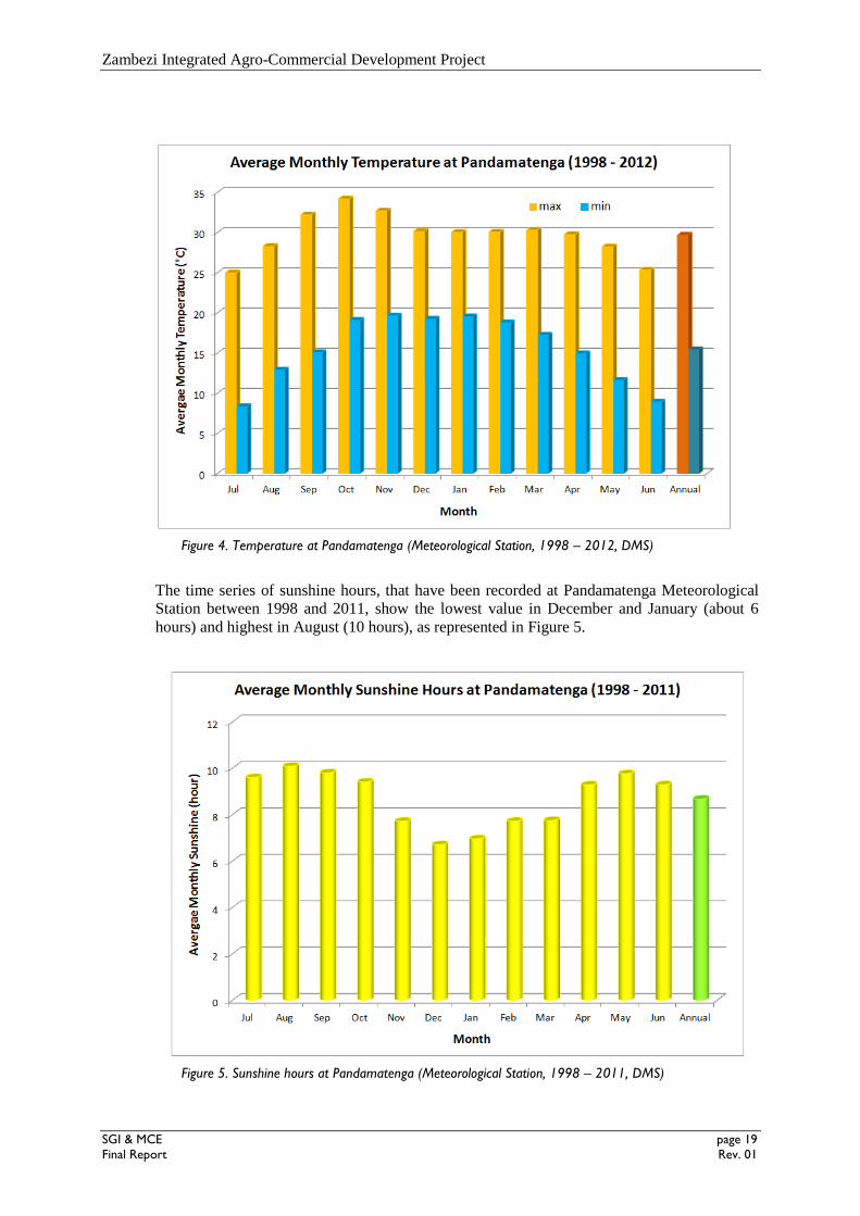
The mean annual temperature in the study area is 22.6 °C according to the measurements at
Pandamatenga Meteorological Station. Maximum monthly temperature is in October with
more than 34 °C while the lower values are in June and July (about 25 °C). The monthly
average of minimum temperature is about 8 °C in July and it reaches 19 °C between October
and February (Figure 4).
Zambezi Integrated Agro-Commercial Development Project
SGI & MCE page 19
Final Report Rev. 01
Figure 4. Temperature at Pandamatenga (Meteorological Station, 1998 – 2012, DMS)
The time series of sunshine hours, that have been recorded at Pandamatenga Meteorological
Station between 1998 and 2011, show the lowest value in December and January (about 6
hours) and highest in August (10 hours), as represented in Figure 5.
Figure 5. Sunshine hours at Pandamatenga (Meteorological Station, 1998 – 2011, DMS)

Zambezi Integrated Agro-Commercial Development Project
SGI & MCE page 20
Final Report Rev. 01
For what concerns relative humidity and wind speed, data are not available in Pandamatenga
therefore the analysis has made reference to the closest station and verifying that the general
meteorological condition can reliably be the same of the study area. These figures and the
evaluation of hydrological analogy have been based upon what is redacted within the
NWMPR.
In case of relative humidity, there are not relevant differences among the stations in the
northern part of Botswana (Maun, Kasane, Shakawe): in fact, the NWMPR includes these
station within an unique region when statistical process for estimating missing climatic data
needs to be applied (for instance, multiple regression of rainfall data).
For the present study data recorded at Maun has been taken into account (Figure 6). The same
monthly trend is shown for measurement at 8 am and 2 pm: during the morning the parameter
ranges from 40% in September to 77% in February, while in the afternoon values vary from
20% to 45%.
Figure 6. Relative humidity at Maun (Airport Station, NWMPR / Botswana National Atlas)
Even information about the wind speed are not available at Pandamatenga therefore the
measurement at Kasane Airport are taken into account: this because, as already mentioned,
Kasane belongs to the same statistical cluster of the study area and it is the closest site.
However, in Kasane the velocity is recorded only at 10 m from the ground thus the
relationship between wind speed at 10 and 2 m has been analyzed for all other stations
(Gaborone, Mahalapye, Francistown, Maun, Shakawe, Ghanzi, Tshane, Tsabong). From this it
comes out that the ratio between velocities at two different height is constantly around 63 –
64%: thus on the basis of this the wind speed at 2 m in Kasane has been estimated.
As it can been noted in Figure 7, wind speed is minimum in January (1.3 m/s at 10 m, 0.8 at 2
m) and reaches the highest value in September (respectively 2.5 and 1.6).

Zambezi Integrated Agro-Commercial Development Project
SGI & MCE page 21
Final Report Rev. 01
Figure 7. Wind speed at Kasane (Airport Station, NWMPR and estimation)
In Pandamatenga evaporation from pan has been recorder daily since 1997 and the resulting
monthly average are shown on Figure 8: measured evaporation ranges between 125 and 170
mm from December to July, then gets higher value having its maximum in October (about 300
mm). The annual cumulative value is about 2,150 mm.
Figure 8. Pan evaporation at Pandamatenga (Meteorological Station, 1997 – 2012, DMS)
Zambezi Integrated Agro-Commercial Development Project
SGI & MCE page 22
Final Report Rev. 01
The following table summarizes the mean monthly values of meteorological parameters that
have been taken into account for agronomic study. Annual values are calculated as monthly
average except for precipitation and evaporation, where cumulate amount has been computed.
Parameter Jan Feb Mar Apr May Jun Jul Aug Sep Oct Nov Dec Annual
Rainfall
(mm) 136 112 65 21 1.0 0.8 0.0 0.0 1.5 23 65 114 539
Temperature
max (°C) 30.0 30.1 30.3 29.8 28.2 25.3 25.0 28.3 32.2 34.2 32.7 30.2 29.7
Temperature
min (°C) 19.5 18.8 17.2 14.9 11.6 8.9 8.3 12.9 15.1 19.1 19.6 19.2 15.4
Temperature
avg (°C) 24.8 24.4 23.8 22.3 19.9 17.1 16.7 20.6 23.6 26.6 26.2 24.7 22.6
Sunshine
(hour) 7.0 7.7 7.7 9.3 9.8 9.3 9.6 10.1 9.8 9.4 7.7 6.7 8.7
Relative
humidity
(%) at 8 am
75 77 75 69 64 64 62 52 40 43 57 68 -
Relative
humidity
(%) at 2 pm
46 45 42 39 29 29 26 21 20 22 32 42 -
Wind speed
(m/s) at 10 m 1.3 1.5 1.5 1.6 2.1 2.1 2.1 2.3 2.5 2.3 1.6 1.5 -
Wind speed
(m/s) at 2 m 0.8 1.0 1.0 1.0 1.4 1.3 1.3 1.5 1.6 1.5 1.0 1.0 -
Pan
evaporation
(mm)
169 151 157 149 144 125 141 191 256 294 217 164 2,157
Table 1 Summary of meteorological parameters for agronomic study
2.4 STATISTICAL ANALYSIS OF RAINFALL
The time series of daily rainfall data measured at Pandamatenga Police Station has been
considered to identify the maximum height for each year (42 years with complete data
between 1962 and 2006). From Figure 9 it can be noted the lower values are around 40 mm;
maximum daily precipitation is less than 60 mm for about 50% of the years, while is more
than 80 mm for a quarter of considered years.

Zambezi Integrated Agro-Commercial Development Project
SGI & MCE page 23
Final Report Rev. 01
Figure 9. Maximum Daily Rainfall at Pandamatenga (Police Station, 1962 – 2006, DMS)
The Gumbel distribution is used to evaluate the statistical distribution of the maximum yearly
values of daily rainfall in order to identify the intensity–duration–frequency (IDF) curves. The
42 values (N = 42) of maximum daily rainfall are listed in descending order thus their
statistical probability can be assessed:
Max Daily
Rainfall (mm) N
Time
Return (Tr)
Exceeding
probability (Ep)
Not exceeding
probability (NEp)
Reduced
variate (Y)
160.0 1 43.0 0.023 0.977 3.749
119.0 2 21.5 0.047 0.953 3.044
114.0 3 14.3 0.070 0.930 2.627
95.0 4 10.8 0.093 0.907 2.326
92.0 5 8.6 0.116 0.884 2.091
92.0 6 7.2 0.140 0.860 1.895
92.0 7 6.1 0.163 0.837 1.728
88.5 8 5.4 0.186 0.814 1.581
84.0 9 4.8 0.209 0.791 1.449
83.5 10 4.3 0.233 0.767 1.329
77.5 11 3.9 0.256 0.744 1.219
76.2 12 3.6 0.279 0.721 1.117
75.0 13 3.3 0.302 0.698 1.022
75.0 14 3.1 0.326 0.674 0.932
72.0 15 2.9 0.349 0.651 0.846
71.0 16 2.7 0.372 0.628 0.765
Zambezi Integrated Agro-Commercial Development Project
SGI & MCE page 24
Final Report Rev. 01
Max Daily
Rainfall (mm) N
Time
Return (Tr)
Exceeding
probability (Ep)
Not exceeding
probability (NEp)
Reduced
variate (Y)
70.4 17 2.5 0.395 0.605 0.687
70.0 18 2.4 0.419 0.581 0.612
70.0 19 2.3 0.442 0.558 0.539
70.0 20 2.2 0.465 0.535 0.469
67.0 21 2.05 0.488 0.512 0.400
66.7 22 1.95 0.512 0.488 0.333
66.2 23 1.87 0.535 0.465 0.267
62.0 24 1.79 0.558 0.442 0.202
58.0 25 1.72 0.581 0.419 0.138
53.0 26 1.65 0.605 0.395 0.075
52.0 27 1.59 0.628 0.372 0.011
50.0 28 1.54 0.651 0.349 -0.052
48.0 29 1.48 0.674 0.326 -0.115
47.0 30 1.43 0.698 0.302 -0.179
47.0 31 1.39 0.721 0.279 -0.244
46.5 32 1.34 0.744 0.256 -0.310
46.0 33 1.30 0.767 0.233 -0.377
43.2 34 1.26 0.791 0.209 -0.447
42.0 35 1.23 0.814 0.186 -0.520
41.8 36 1.19 0.837 0.163 -0.596
41.3 37 1.16 0.860 0.140 -0.678
40.5 38 1.13 0.884 0.116 -0.766
40.0 39 1.10 0.907 0.093 -0.865
37.0 40 1.08 0.930 0.070 -0.979
37.0 41 1.05 0.953 0.047 -1.121
36.0 42 1.02 0.977 0.023 -1.325
Table 2 Statistical elaboration of maximum daily rainfall at Pandamatenga
Then statistical elaboration consists in calculating the following parameters that lead to find
relationship between precipitation heights (h) and return time of storm event:
Xm : mean value of maximum daily rainfall;
Sx : standard deviation of maximum daily rainfall;
Yn : mean value of reduced variate;
Sn : standard deviation of reduced variate;
Gumbel parameters
Xm Sx Yn Sn α ∂
67.0 25.7 0.54 1.16 22.2 54.9
Table 3 Parameters of Gumbel analysis for maximum daily rainfall Pandamatenga

Zambezi Integrated Agro-Commercial Development Project
SGI & MCE page 25
Final Report Rev. 01
Tr (years) 2 5 10 25 50 100
h (mm) 63 88 105 126 142 157
Table 4 Daily rainfall heights related to return time of storm event at Pandamatenga
Being the time series composed of 42 years, rainfall heights with return time of 50 years or
more are not reliable as the others. The resulting values are in line with what has been already
redacted in the previous study related to the Zambezi Integrated Agro-Commercial
Development Project (“Interim Hydrological Report” prepared by TAHAL in 2009) or rather
they are slightly higher, that can be considerate as a conservative output.
Statistical
Analysis
Return time (years)
2 5 10 20 50 100
LN2 59 80.8 95.2 109.1 127.1 140.7
LP3 58.5 80.6 95.8 110.8 131 146.7
Chow 56.7 79.7 94.9 118 157.9 187.9
EVI 59.2 81.6 96.4 110.6 129 142.7
GEV 58.2 80.5 96.3 112.1 133.7 150.9
Table 5 Daily rainfall heights related to return time of storm event at Pandamatenga (TAHAL, 2009)
Measurements of rainfall with duration lower than a day are not available, therefore the
relationship between precipitation heights and return time has been conducted making
reference to the methodological approach proposed in NWMPR (Volume 3). Within this
document it has been redacted values of conversion factor (Table 6) that allow to transform
daily rainfall to shorter storm event (Table 7).
Duration 24h 12h 6h 4h 2h 1h
Ratio with daily rainfall 1.00 0.97 0.90 0.80 0.60 0.40
Duration 1h 45m 30m 15m 10m 5m
Ratio with daily rainfall 0.40 0.36 0.30 0.20 0.14 0.08
Table 6 Conversion factor for daily rainfall heights (NWMPR, 2006)
Rainfall height (mm)
Storm
duration
Return time (years)
2 5 10 25 50 100
24 hours 63 88 105 126 142 157
12 hours 61 86 102 122 137 152
6 hours 57 79 94 113 127 141
4 hours 50 71 84 101 113 126
Zambezi Integrated Agro-Commercial Development Project
SGI & MCE page 26
Final Report Rev. 01
Rainfall height (mm)
Storm
duration
Return time (years)
2 5 10 25 50 100
2 hours 38 53 63 76 85 94
1 hour 25 35 42 50 57 63
45 minutes 23 32 38 45 51 57
30 minutes 19 26 31 38 42 47
15 minutes 13 18 21 25 28 31
10 minutes 9 12 15 18 20 22
5 minutes 5 7 8 10 11 13
Table 7 Rainfall heights related to return time and duration of storm event at Pandamatenga
Figure 10 Intensity–duration–frequency relationship for storm event with duration more than one hour

Zambezi Integrated Agro-Commercial Development Project
SGI & MCE page 27
Final Report Rev. 01
Figure 11 Intensity–duration–frequency relationship for storm event with duration less than one hour
Using the above described relationship, the related storm runoff will be determined and the
drainage system will be designed (paragraph 6).
Zambezi Integrated Agro-Commercial Development Project
SGI & MCE page 28
Final Report Rev. 01
3 HYDROGEOLOGY
3.1 GENERAL HYDROGEOLOGICAL FRAMEWORK
The geology and climate, past and present, are important factors that influence the
groundwater resources of Botswana (Dep. of Surveys and Mapping, 2001). Groundwater in
Botswana is limited, both in quantity and quality and is unevenly distributed over the country.
Groundwater collects in aquifers and is abstracted through well fields.
Only a small part of the groundwater resources can be economically abstracted due to high
abstraction costs, low yields, poor water quality and remoteness of aquifers in relation to
consumers centres (SMEC et al, 1991, Masedi et al, 1999). The estimated mean annual
recharge is 2.7 mm being zero in western Botswana to 100 mm in the north.
The extractable volume of groundwater in Botswana is estimated to be about 100.000 Mm3
(Khupe, 1994). But only 1% of this amount is rechargeable by rainfall because of the semi-
arid climate characterised by low rainfall amount and high rates of evaporation as well as the
nature of geology of aquifers (Ayoade, 2001).
According to Ayoade (2001) four types of aquifers are found in Botswana:
a) Fractured aquifers, which cover 27% of the country, are found in the crystalline
bedrocks of the Archaen Basement in the east and in the Karoo Basalt. These have
low yields with the median yield ranging between 2 and 10 ma per hour.
b) Fractured porous aquifers, which cover 37% of the country, are found in Ntane and
Ecca sandstones as well as in arkoses in the Karoo Formation. These aquifers have the
highest yields.
c) Porous aquifers, which cover 35% of Botswana, occur in sand rivers, alluvium and the
Kalahari beds (presumable aquifers existing in the zone of “Chobe Irrigation Area”).
These are usually high yielding and have a median yield ranging between 10 and 300
m3 per hour.
d) Karstified aquifers occur in the dolomite areas in southwestern parts of Botswana as
well as in other areas in Lobatse, Ramotswa and Kanye. Karstified aquifers account
for only 1% of the land area of Botswana. These aquifers have a median yield of 4-20
m3 per hour.
Groundwater is located at great depth except in a few areas receiving regular floods or with
permanent water bodies. The depth varies over the country from less than 40 m in the north
and east (where is located the Chobe Irrigation Area) to well over 60 m in the drier central
and south-western parts. The borehole technology has opened up very deep groundwater
deposits.
Over a large part of Botswana, borehole yields are poor to fair with average yields being less
than 4 m3 per hour. In only a few areas are the average borehole yields in excess of 8 m
3 per
hour.
In eastern and northern Botswana where is located the “Chobe Irrigation Area”, recharge
should increase to between 20 and 100 mm/yr, depending on local geology and
geomorphology.
Zambezi Integrated Agro-Commercial Development Project
SGI & MCE page 29
Final Report Rev. 01
Figure 12. Map of Average depth of Groundwater (Department of Surveys and Mapping, 2001)
Information on groundwater recharge is of fundamental interest for any hydrogeological
study, usually displayed as a layer for assigning aquifer productivity, or as an inset map.
Recharge is a complex process governed by a number of controlling factors as that are highly
variable in space and time as rainfall, evapotranspiration and unsaturated zone.
However, Döll & Fiedler (2008) have developed an algorithm to estimate the diffuse
groundwater recharge at the global scale, with a spatial resolution of 0.5°. This algorithm has
been adopted to create a recharge layer for the African Hydrogeology Map and for the World
Hydrogeological Map.
In Figure 13, it appears the recharge layer of the Hydrogeological map designed for the
Southern African Development Community (SADC Project – Final Report March 2010). In
the zone of Chobe Irrigation Area, the Groundwater potential is classified as: “High, but
variable (occasional or no recharge)”.

Zambezi Integrated Agro-Commercial Development Project
SGI & MCE page 30
Final Report Rev. 01
Figure 13. Map of Mean Annual Recharge (Doll and Fiedler, 2008)
3.2 DATA GATHERING AND PREVIOUS STUDY
For the local geological and hydrogeological characterization of Irrigation Area, the
Consultant analyzed even the results of previous local studies, as the surveys and shallow pits
already performed for “Geotechnical Investigation for the Preliminary Design on the
utilization of the water resource of the Chobe/Zambezi river” redacted by Geotechnics
International Botswana in June 2013, concerning the track of pipeline transfer in the
Pandamatenga area for a total length of about 67 km.
This study was consisted of n° 4 boreholes drilled up to 15 m. u.g.l. (DH1, DH2, DH3 and
DH4 as represented in Figure 14).

Zambezi Integrated Agro-Commercial Development Project
SGI & MCE page 31
Final Report Rev. 01
Figure 14. Layout of previous local geotechnical investigations (Consultant’s elaboration, 2014)

Zambezi Integrated Agro-Commercial Development Project
SGI & MCE page 32
Final Report Rev. 01
Depth (m) Lithotype Average SPT
(0.0 ÷ 3.0) m. Black, Stiff, Intact Clay 25
(3.0 ÷ 4.5) m. Completely weathered, highly fractured, soft Basalt 28
(4.5 ÷ 7.3) m. Highly weathered, highly fractured, soft Basalt 62
(7.3 ÷ 11.0) m. Highly to moderately weathered, medium fractured,
soft to moderately strong, Basalt
(11.0 ÷ 15.0) m. Moderately weathered, medium fractured,
moderately strong, Basalt
Depth of water Water table encountered at depth of 8.3 m.
Table 8 Stratigraphic description regarding soils in borehole DH1
Depth (m) Lithotype Average SPT
(0.0 ÷ 2.0) m. Sandy Clay
(2.0 ÷ 10.0) m. Very dense, slightly cemented silty sand
with traces of calcrete gravel 38
(10.0 ÷ 15.0) m. Very dense, slightly cemented silt sand 25 refusal
Depth of water No water table encountered
Table 9 Stratigraphic description regarding soils in borehole DH2
Depth (m) Lithotype Average SPT
(0.0 ÷ 10.5) m. Medium dense to very dense silty sand 42
(10.5 ÷ 12.0) m. Highly weathered, highly fractured,
soft basalt
(12.5 ÷ 15.0) m. Moderately weathered, medium fractured,
moderately strong, basalt 50
(12.0 ÷ 15.0) m. Moderately weathered, medium fractured
Depth of water No water table encountered
Table 10 Stratigraphic description regarding soils in borehole DH3
Depth (m) Lithotype Average SPT
(0.0 ÷ 1.5) m. Silty Sand, aeolian
(1.5 ÷ 12.0) m. Medium dense to very dense Silty Sand
with traces of calcrete gravel 48
(12.0 ÷ 15.0) m. Very dense, Sandy Calcrete
Depth of water No water table encountered
Table 11 Stratigraphic description regarding soils in borehole DH4
For a better hydrogeological framework of the study area, were examined the considerations
of the Hydrogeological Survey about “Zambezi Integrated Agro-Commercial Development
Project”, where n° 25 exploration boreholes (BH) were drilled in the area that is located
midway between Kasane and Pandamatenga, about 30 km to the north of “Chobe Irrigation
Area” (see figure below).

Zambezi Integrated Agro-Commercial Development Project
SGI & MCE page 33
Final Report Rev. 01
Figure 15. Map of Hydrogeological Survey results (Consultant’s elaboration, 2014)
The depth of the boreholes varied from 14 m to 37 m under ground level, furthermore it is
realized the execution of water quality laboratory analysis, calculation of groundwater regime,
absolute water level and flow direction with indication of the possible exploitable aquifers.
The general results can be summarized in the following tables.
Zambezi Integrated Agro-Commercial Development Project
SGI & MCE page 34
Final Report Rev. 01
Table 12 Depth of Static Water Level upon completion of drilling and after several days (TAHAL
Group Hydrogeological Survey, 2008)

Zambezi Integrated Agro-Commercial Development Project
SGI & MCE page 35
Final Report Rev. 01
Table 13 The thickness of the various beds from surface downward (TAHAL Group Hydrogeological
Survey, 2008)
It can be observed how the depth of groundwater varies between 10 m and 20 m below ground
level, the flow direction is from east to towards west vice versa the depth of groundwater
level.
3.3 PLANNING OF FIELD SURVEY
In the zone of Chobe Irrigation Area, the area looks flat with a slight slope from NE to SW,
the location of boreholes has been established choosing them among the ground control point
(where ground level will better defined) and taking into account the general trend of water
table or rather having 3 points that allows estimating the gradient of water table.
The following image shows the location of the borehole that were realized.

Zambezi Integrated Agro-Commercial Development Project
SGI & MCE page 36
Final Report Rev. 01
Figure 16. Layout of realized borehole for hydrogeological survey (Consultant’s elaboration, 2014)
Thus this investigation was accomplished with n. 3 borehole reaching 40 m under the ground
level. The resulting depth of groundwater within the “Chobe Irrigation Area” varies between
31.10 m in BH-1 and 36.67 m in BH-3 below surface, while in BH-2 the depth is certainly
greater than 40.00 m, because at less depth the hole is resulted dry.
At North of irrigation area, in the borehole DH1 the useful measured depth was 8.30 m below
ground level, (in the boreholes DH2, DH3 and DH4 no water table was encountered to a
depth of 15 metros under ground level).
The depth of the static water level, the elevation of the reference points and the absolute water
level are presented in the next table.
Borehole No.
Date of Survey
Depth of S.W.L. (u.g.l.)
- m -
Elevation of Ground (a.s.l.)
- m -
Absolute Water Level (a.s.l.)
- m -
BH-1 June 2014 31.10 1079 1047.90
BH-2 June 2014 > 40.00 1058 < 1018
BH-3 June 2014 36.67 1065 1028.23
DH-1 June 2013 8.30 1075 1066.70
Table 14 Available values of Static Water Level and Absolute Water Level

Zambezi Integrated Agro-Commercial Development Project
SGI & MCE page 37
Final Report Rev. 01
So, with the available data that are measured in the same autumn period (June 2013 and June
2014), it can be concluded that the flow direction is from north-east towards south-west (see
also next figure). Because the water table is so deep, it is reliable that agricultural practises
would not cause such a raising to make in contact between surface and groundwater thus
avoiding any risk of contamination by fertilizers.
Figure 17. Map of Absolute Water Level and Flow Direction (Consultant’s elaboration, 2014)

Zambezi Integrated Agro-Commercial Development Project
SGI & MCE page 38
Final Report Rev. 01
4 ONFARM IRRIGATION SYSTEM DESIGN
4.1 PLANNING OF IRRIGATION SYSTEM
The step-by-step procedure taken in planning and design of irrigation system are inventory of
available resources and operating conditions, topographic map of the area, water supply –
source availability and dependability, climatic condition, power source, crop selection and
water supply level.
As it was mentioned in the TOR, the key focus of the infrastructure component activities was
the planning of water use for irrigation considering the potable water demand as a subsequent
step. In addition, it was already noted in the TOR that pressurized irrigation systems could be
considered very advantageous for this project.
Based on this and taking several selection criteria, centre pivot sprinkler system was selected
for sandy clay loam, sandy loam and loamy sand soils and drip irrigation system for sandy
soils (details in paragraph 4.2). The planning and design of these two systems were performed
for the water distribution and irrigation system considering the technical feasibility, economic
viability, social acceptance and environmental sustainability.
The design of irrigation system was carried out on-demand based of irrigation requirements.
Then, the network layout was designed to give inputs on most efficient ways of connecting all
the users.
4.1.1 Design criteria
In principle, the first step in the preliminary design phase was the collection of basic farm
data. These are topographic map showing the proposed irrigated area, with contour lines,
farm and field boundaries and water source or sources, power points- such as electricity lines
in relation to water source and area to be irrigated, roads and other relevant general features
including obstacles.
Moreover, data on water resources (quantity and quality) over time, the climate of the area and
its influence on the water requirements of the selected crops, the soil characteristics and their
suitability to the crops and irrigation system proposed, the types of crops intended to be
grown and their adaptability to both the climate and the area were collected.
The next step was analyzing the farm data in order to determine the following preliminary
design parameters: peak and total irrigation water requirements, infiltration rate of soils to be
irrigated, maximum net depth of water application per irrigation, irrigation frequency and
cycle, gross depth of water application and preliminary system capacity.
4.1.2 Land resource
As per the results of the soils analysis and based on the field investigation and laboratory
results, seven land units have been classified as shown in the following table.
The soil physical and chemical properties used for selection of pressurized irrigation system
and design of centre pivot and drip irrigation system are shown in Table 16 and paragraph 9.1.

Zambezi Integrated Agro-Commercial Development Project
SGI & MCE page 39
Final Report Rev. 01
Mapping
Unit Soil/Land Unit Description
Area
ha %
ZA1/1
1
Flat almost flat, very deep, moderately well drained, very
dark gray to gray color, sandy clay loam, developed on
lacustrine 0-1.5% slopes: Soil HypereutricVertisols
(Vreuh)
5,512 12.13
ZA1/2
2
Flat, moderately deep, well drained, Very dark gray -
Dark grayish brown color, sandy loam texture,
developed on lacustrine, 0-1% slopes: soils
HypocalcicVertisols (VRccw)
6,656 14.56
ZA2/3
3
Flat almost flat, very deep , somewhat excessively
drained, dark reddish brown to light brownish gray
color, loamy sand texture, developed on sandveld, slopes
0-1.5%, Soils: HypoferalicArenosols (ARflw )
1,903 4.19
ZA2/4
4
Flat almost flat, very deep, excessively drained, dark
grayish brown to yellowish brown color, developed on
sandveld, deposit, sand texture, slope o-2% soils:
21,300 47.0
ZA5
Flat almost flat, very deep, excessively drained, dark
grayish brown to yellowish brown color, developed on
sandveld, deposit, sand texture, slope o-2% soils:
10,000 22
ZA6 Settlement 10.8 0.02
ZA7 Quarry Site 4.65 0.01
Table 15 Classified area as per the textural analysis
Soil type Infiltration (cm/hr) HC (m/day) AW (mm/m)
Sandy Clay loam 2.9 2.7 97.2
Sandy Loam 4.73 2.54 85.11
Loamy Sand 10.9 6.37 76.85
Sand 26.57 19.11 61.92
Table 16 Average values of soil physical properties of the study area
4.1.3 Water resource
As per the TOR, total water extraction is estimated at 495 million cubic meters per year. The
National Water Authority will use about 150 million cubic meters, with the remaining 345
million cubic meters, being used for the proposed agricultural project. The irrigation water
would be pumped from a reservoir with a design capacity of 2.0 million m³.
As underlined in the National Master Plan for Arable Agriculture and Dairy Development
(NAMPAADD), “since water is a scarce resource in Botswana, farmers will be encouraged to
use water efficient technologies for irrigation.” In light of this, the Client perceives
minimizing water losses in the conveyance, distribution and application as an important
consideration for the present project.
Hence, taking into account the latest trends in the irrigation sector as well as indications
provided by the ToR, the development of a pressurized irrigation system for the project area
has been considered. Moreover, it was given that the design discharge from the pump station
to reservoir R2 at Pandamatenga is 23,300 l/s.

Zambezi Integrated Agro-Commercial Development Project
SGI & MCE page 40
Final Report Rev. 01
4.2 OPTIONS IDENTIFICATION AND ASSESSMENT
The principal objectives of this component of the project are:
Assess different alternatives for the development of a water distribution / irrigation
system in the area,
select the most suitable option - taking into account the criterion:
− viability
− suitability for local conditions
prepare a corresponding conceptual design and implementation plan.
Irrigation technologies depend on specific chemical, biological and physical conditions of
water and soil as well as types of cultivated crops. These, together with the objective of an
efficient use of available resources and irrigation system productivity (attained by optimizing
investment and operation and maintenance cost), imply setting a number of determinant
parameters that guide the assessment of alternatives for the irrigation and water distribution
systems development.
Recognizing the pressurized irrigation system suggested by MoA and as per the given TOR
and technical proposal, the following two methods of pressurized irrigation systems were
selected and evaluated.
Sprinkler irrigation system
Drip/trickle irrigation
Sprinkler irrigation system has the following advantages:
Uniform distribution of water
Accurate measurement of the applied water, rendering high water use efficiency
Eliminates excessive losses from deep percolation, surface runoff and conveyance
losses
Land with irregular topography can be irrigated by sprinklers without much leveling
and land preparation
Can be used on soils with low water holding capacity
Can be used on sloping lands
Does not require field channels and thus more areas become available for crop
production
Possibilities of fertigation and chemigation
can be used for almost all crops and on most soils
Feasibility of frequent, small water amount applications for germination, cooling,
frost protection, etc.
The closed water delivery system prevents contamination of the irrigation water.
Some disadvantage of the sprinkler irrigation system, which will be corrected through design
and management, are as follows:
High initial investment
Energy cost is usually high as water is pumped under pressure.
Design, planning and operation of sprinkler system require good technical expertise.
Sensitivity to wind conditions
Water losses by evaporation from soil surface and plant canopy, if wetted.
Induction of leaf diseases in over-head application.
Hazard of salt accumulation on wetted foliage in overhead application.
Leaf burns and washout of pesticides from the foliage in overhead application.
Interference of irrigation with various farm activities like tillage, spraying, harvest,
etc.

Zambezi Integrated Agro-Commercial Development Project
SGI & MCE page 41
Final Report Rev. 01
For what concerns adaptability, some of the conditions, which favours sprinkler irrigation, are
as follows.
Shallow soils the topography of which prevents proper levelling for surface irrigation
methods
Land having steep slopes and easily erodible soils.
Irrigation stream too small to distribute water efficiently by surface irrigation.
Undulating land too costly too level sufficiently for good surface irrigation.
Soils with low water holding capacities and shallow rooted crops, which require
frequent irrigation.
Automation and mechanization are practical.
Higher application efficiency can be achieved by properly designed and operated
systems.
Good clean supply of water, free of suspended sediments, is required to avoid
problems of sprinkler nozzle blockage and spoiling the crop by coating it with
sediment.
In the options assessment process, the following decision making parameters were used:
available water sources,
soils and topography,
climate and crop,
capital and labour,
energy,
social aspects and policies,
socio-economic aspects,
health aspects and
environmental aspects.
4.2.1 Alternatives of different pressurized irrigation system
Primarily there are two major classifications of sprinkler irrigation systems. These are
Conventional systems (periodic move & Solid set) and Continuous sprinkler machines.
Different irrigation systems are further classified in the following manner.
Zambezi Integrated Agro-Commercial Development Project
SGI & MCE page 42
Final Report Rev. 01
Hand move sprinkler system
Figure 18 Schematic functioning of hand move sprinkler system

Zambezi Integrated Agro-Commercial Development Project
SGI & MCE page 43
Final Report Rev. 01
Figure 19 Example of continuous type sprinkler irrigation system
4.2.2 Selection of continuous over conventional sprinkler system
Comparing the conventional sprinkler method with that of the continuous system, the
following parameters were envisaged.
Continuous system is labour-saving as compared to high labour costs to move the
conventional set
Easily automated, fertigation and chemigation is possible- applies chemicals and
fertilizers inexpensively, accurately and at any stage of the crop growth.
Largeness of the command area leads to the use of continuous type of sprinkler
system
Periodic move systems apply water for a set time while stationary before moving to
the next position but, the continuous move system apply water while in motion
Continuous move system is highly efficient and environmentally sound giving less
run-off and disposal of water to down stream
Efficient water usage—minimizes deep percolation loss and evaporation through
timely and precise applications.
Uniform coverage—irrigates uniformly throughout the entire field
4.2.3 Centre pivot irrigation system
Self-propelled sprinkler system rotates around the pivot point and has the lowest labour
requirements of the systems considered. The water source for this system, a well or buried
pipeline, is located at the centre of the field and delivers water to the pivot arm.
The rotation of the pivot arm results in the pattern of circular irrigated areas. In the case of
centre pivot irrigation without corner system, π/4 = 79% of the square area is irrigated
applying irrigation water in circles (vs. squares), as presented in the following figures.
Zambezi Integrated Agro-Commercial Development Project
SGI & MCE page 44
Final Report Rev. 01
Figure 20 Example of alignment of center pivot
Figure 21 Center pivot sprinkler working in the field
Sprinkler nearest the pivot point may discharge only a fine spray; constant radial velocity but
variable tangential speeds (fastest at periphery). The water application amount is controlled by
the speed of rotation.
Centre pivots are adaptable for any height crop and are particularly suited to lighter soils.
They are generally not recommended for heavy soils with low infiltration rates. Computerized
control panels allow the operator to specify speed changes at any place in the field, reverse the
pivot, turn on auxiliary pumps at a specified time and use many other features.
The low per hectare cost of large centre pivot systems, the limited labour requirements and the
low energy requirements of pivot systems using spray nozzles are the main reasons for the
popularity of these systems. Centre pivot systems equipped with nozzles and drop pipes,
placing the nozzles just above the crop canopy, are very useful under windy conditions.

Zambezi Integrated Agro-Commercial Development Project
SGI & MCE page 45
Final Report Rev. 01
4.2.4 Centre pivot with corner attachment and/or end guns
Corner attachment systems that allow irrigation of most of the corner areas missed by a
conventional centre pivot system are available. Depending on the method of corner irrigation,
pivot systems with corner attachments will irrigate additional area of quarter section.
However, in the case of centre pivot with corner attachment and /or end guns, generally the
corner span alone costs about half as much as the rest of the pivot, thereby increasing the
capital cost per hectare. It is because of this reason, we planned to take centre pivot without
corner or end gun (Figure 22).
Figure 22 Example of center pivot with corner attachment
4.2.5 Linear move sprinkler
The linear move (sometimes called a lateral move) irrigation system is built the same way as a
center pivot; that is, with moving towers and spans of pipe connecting the towers. The main
difference is that all the towers move at the same speed and in the same direction.
Water is pumped into one of the ends or into the centre. Water can be supplied to the linear
move through a canal or by dragging a supply hose that is connected either to a main line or
by connecting and disconnecting from hydrants as the linear moves down the field. Field must
be rectangular.
Typically gives high application uniformity. Usually fed by open ditch with moving pump,
requiring very small (or zero slope) in that direction. It can also be fed by dragging a flexible
hose, or by automated arms that move sequentially along risers in a mainline.
It does not have problem of variable tangential speeds as with centre pivot. However, due to
the lateral movement, powering a linear with electricity is difficult. Usually, a diesel motor
with a generator is mounted on the main drive tower and supplies the power needed to operate
the irrigation system.
It requires the source of water to be available all along one edge of the field. Water supply
system is more complex for a linear-move system than a centre pivot because the distribution
system delivers water along the entire length of one side of the field instead of only at the
center (Figure 23).

Zambezi Integrated Agro-Commercial Development Project
SGI & MCE page 46
Final Report Rev. 01
Figure 23 Linear move supplied to the linear move through a canal
4.2.6 Side role sprinkler
The side roll (sometimes called a wheel roll) system, consists of a lateral, usually a quarter
mile long, mounted on wheels with the pipe acting as an axle. Side roll systems also are
adapted only to short crops; have medium labour requirements, moderate initial investment,
medium operating pressure and generally rectangular field requirements irrigating limited
area.
The side roll is better adapted to heavy textured soils than other continuous moving system.
This type of system essentially evolved out of a labor shortage to move the hand-move lines.
An entire length of side- roll line is moved by a small derive motor installed in the center of
the line.
In general, since, the soils of the project area are not heavy textured soil and the area is very
large; side roll sprinkler type is not selected (Figure 24).
Figure 24 Side roll sprinkler system

Zambezi Integrated Agro-Commercial Development Project
SGI & MCE page 47
Final Report Rev. 01
4.2.7 Big gun sprinkler
Gun traveller sprinkler is a high capacity sprinkler fed with water through a flexible hose;
mounted on self-propelled chassis and travels along a straight line while watering. It has a
single large diameter nozzle, which sprays large volumes of water reaching in a circular
pattern. Long flexible hose with high head loss may reel up the hose or be pulled by a cable on
a trailer.
The travelling big gun system uses a large-capacity nozzle and high pressure to throw water
out over the crop as it is pulled through an alley in the field. It is particularly adaptable to
various crop heights, variable travel speeds, odd-shaped fields and rough terrain. The big gun
requires a moderate initial investment, more labour and higher operating pressures than centre
pivots and linear moves (Figure 25).
Figure 25 Big gun sprinkler system
4.2.8 Drip irrigation system
Drip irrigation system is the method of watering at the plant location frequently with volume
of water approaching the consumptive use (CU). The spacing of emitters is much less than
that of sprinklers and the pipe distribution network is working under low pressure.
In drip irrigation system, not all areas are irrigated and hence, the area irrigated is only
accounted for. Moreover, Emitter spacing is not a function of wind in the case of drip
irrigation system. It is used on almost any type of soil including Clay soil, marginal/infertile
soil and stony soils.
In drip irrigation, system evaporative component is reduced as only limited area of the soil is
wetted and the limited wetted area results in reduced weed growth. It gives accurate water
distribution resulted in high water application efficiency.
The slow rate of water application improves the penetration of water into problematic soils,
keeping the root zone with a high water potential. It is water saving technology with less
energy and operating cost (Figure 26).

Zambezi Integrated Agro-Commercial Development Project
SGI & MCE page 48
Final Report Rev. 01
Figure 26 Layout of drip irrigation system showing the significance of reduced/wetted area as compared to
the total area
4.2.9 Final selection of irrigation system
Out of the above five alternative continuous sprinkler irrigation systems, the center pivot has
been selected according the following justifications:
1. Since centre pivot is fully / semi automated system with computerized control panels,
it is labour saving system.
2. Centre pivot sprinkler system is suitable for light soils with high intake rates, hence
the soils of the study area fulfil this requirement
3. The water source for this system, whether a well or buried pipeline, is located at the
centre of the field and delivers water to the pivot arm.
4. The cost of the moving centre pivot laterals depends on its length. Long laterals are
cheaper (per unit area).
5. The pivot arm is rotated by hydraulic or electric derive motors connected to the
wheels at the intermittent towers. Hence, linear move type requires continuous move
electricity power, open channel or long hoses to supply water along the lateral, it is
rejected to use
6. Linear move requires the source of water to be available all along one edge of the
field.
7. Water supply system is more complex for a linear-move system than a centre pivot
because the distribution system delivers water along the entire length of one side of
the field instead of only at the centre.
8. Gun type system irrigates small plot areas by pulling with additional labour, but the
study area is very large which could not be suitable for gun type system.
9. Side roll type of sprinkler is suitable for heavy clay soils and covers small area
coverage, hence no clay soil is available and the study area is very large, it is rejected
10. Drip irrigation may be another alternative for fruit crops in a sand soils and is adapted
Therefore, based on the above justifications, the planning and design work of irrigation for the
study area was done with centre pivot continuous irrigation system for those identified
suitable soils, sandy clay loam, sandy loam and loamy sand. In addition to this, Drip irrigation
system was evolved for perennial fruit crop, i.e. mango on sandy soils.

Zambezi Integrated Agro-Commercial Development Project
SGI & MCE page 49
Final Report Rev. 01
4.3 CROP WATER REQUIREMENTS
Crop water requirements (CWR) encompass the total amount of water used in
evapotranspiration. Irrigation requirements (IR) refer to the water that must be supplied
through the irrigation system to ensure that the crop receives its full crop water requirements.
The four procedural steps involved in the calculation of crop water and irrigation water
requirements are:
Calculation of reference evapotranspiration (ETo) based on meteorological parameters
collected from the near-by meteorological stations.
Crop coefficients for three annual crops, Maize, Wheat, and Soybeans and two
perennial crops, Alfalfa and fruit crop (Mango) for full-fledged irrigation during the
dry season and also during the wet season, three annual crops (Sorghum, sunflower
and beans) for supplementary irrigation.
Determination of monthly crop water requirements (ETc) depending upon the
cropping patterns and local conditions.
Determination of Irrigation water requirements/demand using calculated effective
rainfall of the area
The crop water requirement and irrigation water demand for all selected crops have been
estimated using 80% dependable rainfall on a monthly basis and the FAO’s CROPWAT
computer model (FAO, 1996).
4.3.1 Reference crop evapotranspiration
The estimation of crop water requirement normally needs the analysis of climatic data and
agronomic practice of the proposed project area. The reference crop evapotranspiration (ETo),
that is analyzed using the modified Penman Method, gives the effect of climate on crop water
requirement. The monthly climate data of the study area collected from the following sources.
Parameter: Rainfall
Source: Department of Meteorological Services
Parameter: Temperature (Max and Min)
Source: Department of Meteorological Services
Station: Pandamatenga Met. Stn.
Years: 1998 - 2012
Parameter: Relative humidity (at 8 am and 2 pm)
Source: National Water Master Plan - Volume 3
Station: Maun Airport
Years: 1965 - 1998 (approx)
Parameter: Wind speed (at 10 and 2 m)
Source: National Water Master Plan - Volume 3
Station: Kasane Airport
Years: 1982 - 2000 (approx)
Parameter: Monthly Temperature (Max and Min)
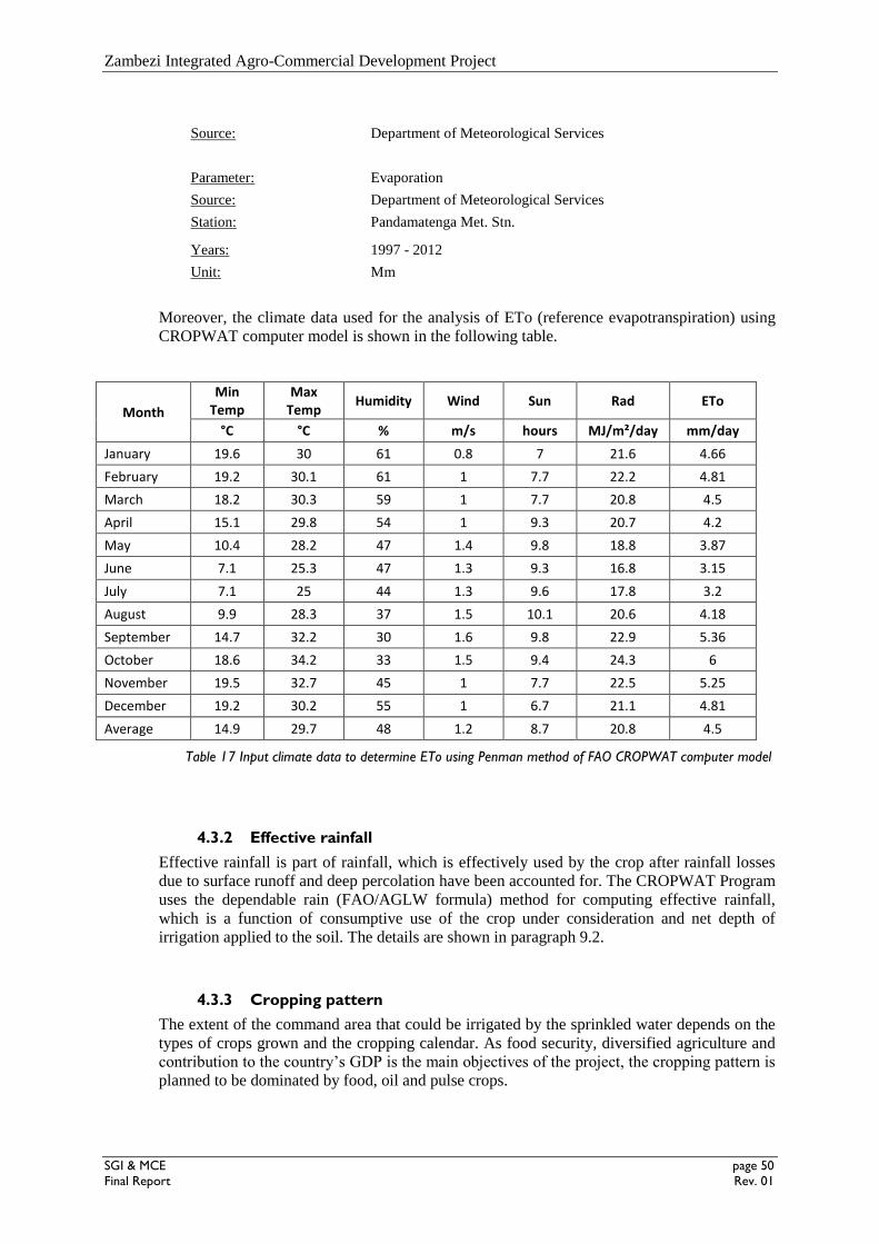
Zambezi Integrated Agro-Commercial Development Project
SGI & MCE page 50
Final Report Rev. 01
Source: Department of Meteorological Services
Parameter: Evaporation
Source: Department of Meteorological Services
Station: Pandamatenga Met. Stn.
Years: 1997 - 2012
Unit: Mm
Moreover, the climate data used for the analysis of ETo (reference evapotranspiration) using
CROPWAT computer model is shown in the following table.
Month
Min Temp
Max Temp
Humidity Wind Sun Rad ETo
°C °C % m/s hours MJ/m²/day mm/day
January 19.6 30 61 0.8 7 21.6 4.66
February 19.2 30.1 61 1 7.7 22.2 4.81
March 18.2 30.3 59 1 7.7 20.8 4.5
April 15.1 29.8 54 1 9.3 20.7 4.2
May 10.4 28.2 47 1.4 9.8 18.8 3.87
June 7.1 25.3 47 1.3 9.3 16.8 3.15
July 7.1 25 44 1.3 9.6 17.8 3.2
August 9.9 28.3 37 1.5 10.1 20.6 4.18
September 14.7 32.2 30 1.6 9.8 22.9 5.36
October 18.6 34.2 33 1.5 9.4 24.3 6
November 19.5 32.7 45 1 7.7 22.5 5.25
December 19.2 30.2 55 1 6.7 21.1 4.81
Average 14.9 29.7 48 1.2 8.7 20.8 4.5
Table 17 Input climate data to determine ETo using Penman method of FAO CROPWAT computer model
4.3.2 Effective rainfall
Effective rainfall is part of rainfall, which is effectively used by the crop after rainfall losses
due to surface runoff and deep percolation have been accounted for. The CROPWAT Program
uses the dependable rain (FAO/AGLW formula) method for computing effective rainfall,
which is a function of consumptive use of the crop under consideration and net depth of
irrigation applied to the soil. The details are shown in paragraph 9.2.
4.3.3 Cropping pattern
The extent of the command area that could be irrigated by the sprinkled water depends on the
types of crops grown and the cropping calendar. As food security, diversified agriculture and
contribution to the country’s GDP is the main objectives of the project, the cropping pattern is
planned to be dominated by food, oil and pulse crops.

Zambezi Integrated Agro-Commercial Development Project
SGI & MCE page 51
Final Report Rev. 01
However, for sustainability and profitability of the project, the crop mix is also considering
high value crops including fruit and forage crops. Besides, it must be noted that:
the pattern is based on farmers’ current practices;
the total suitable area identified by the soils study and latter adjusted by the irrigation
engineers is 15,000 ha (both for rain-fed & irrigated crops);
the choice of irrigated crops is based on food and cash value mix.
The cropping pattern developed by the agronomist is shown in following table.
Crop Type Wet Season
(Nov-Mar)
% of area coverage
Dry season (May- Sep)
% of area coverage
Remarks
Grain crops Sorghum 45* Maize Wheat
40* 30*
Oilseed Sunflower 25* Soybeans 20*
Pulses Beans 20*
Fruit trees Citrus, Mango 40** Mango 40** Grows all
year round
Forage Alfalfa 10* Alfalfa 10* Grows all
year round
* Area based on suitability
** Area included on improved management basis (40% of 25,000 ha)
Table 18 Cropping patterns for wet and dry season
Moreover, the cropping patterns for both wet season (Sorghum 6, 750 ha, Sunflower, 3,750 ha
and Beans, 3,000 ha) and dry season (Maize, 6,000 ha, Wheat, 4,500 ha, Soybean 3,000 ha,
Alfalfa 1, 5000 ha and Fruit, Mango 10,000 ha) along with crop water demand are presented
in paragraph 9.2.
4.3.4 Net irrigation requirements
The net irrigation water requirement is determined based on the crop water requirement and
effective rainfall. The scheme water requirements are computed as aggregate of the crop water
requirement. The irrigation schedules for each crop are computed based on the type of soils
and the crop growth stage.
A detailed methodology, calculations, analysis and summary of the crop and irrigation water
demand is given in agronomy report of this study. The details of the net irrigation for both
supplementary and full-fledged irrigated crops are given in paragraph 9.2.
4.3.5 Irrigation efficiency
The amount of water stored in the root zone is estimated as the net irrigation dose. However,
during the irrigation process, considerable water loss occurs through seepage, deep
percolation, etc. The amount lost depends on the efficiency of the system.
Irrigation efficiency is the efficiency of the total process of irrigation from the source of the
water to the point where the water becomes available in the root zone of the plant. To account

Zambezi Integrated Agro-Commercial Development Project
SGI & MCE page 52
Final Report Rev. 01
for losses of water incurred from the sprinkler and drip systems, an efficiency factor should be
included when calculating the gross irrigation requirements. Hence, 80% application
efficiency was taken for designing sprinkler and 90% for drip irrigation system in the project
area.
4.3.6 Gross irrigation requirements
The gross irrigation requirement is computed by dividing the net irrigation requirement by the
respective irrigation efficiency for both centre pivot and drip irrigation systems. Moreover,
gross irrigation requirement for all crops under study is shown in paragraph 9.2.
4.3.7 Irrigation duty
The peak requirement in terms of duty in litres/sec/ha was calculated to determine the
command area and system capacity of the conveyance and distribution systems based on the
estimated monthly gross irrigation demand. Details of irrigation duty calculations are given in
agronomy report.
The irrigation water duty was determined from the peak irrigation duty of the peak months of
four crops in the case of sprinkler irrigation. Then based on the weighted average area method,
the irrigation duty was calculated as 0.71 l/s/ha. This is based on 24 hours irrigation duty of
the system. This does not mean that the system is working for 24 hours. However, operation
time is 22 hrs in the case of centre pivot sprinkler irrigation system.
The procedure on how the peak irrigation duty for centre pivot irrigation system was
determined using weighted average area method is as follows:
Selected crops for center pivot with thir respective area are: Maize (6,000 ha) , Wheat ( 4,500
ha), Soybean ( 3,000 ha) and Alfalafa ( 1,500 ha).. The respective peak irrigation duty during
the peak months are , 0.71 l/s/ha on September, 0.62 l/s/ha August, 0.82 l/s/ha September and
0.77 l/s/ha October.. The weighted average area irrigation duty is calculated as:
Taking the weighted average area irrigation duty of 0.71 l/s/ha, the gross irrigation depth was
determined as
The net irrigation depth was calculated as
Where,

Zambezi Integrated Agro-Commercial Development Project
SGI & MCE page 53
Final Report Rev. 01
0.116 = conversion factor from l/s/ha to mm/day
dgross = net irrigation depth, mm/day
dnet = net irrigation depth, mm/day
Details are given on Paragraph 9.2.
Moreover, irrigation duty for drip irrigation system was determined as 0.64 l/s/ha on 24 hrs
basis from the peak month of October for Mango crop. However, the operation time for drip
irrigation system is designed as 21 hrs. The detail calculation procedure is shown on
agriculture report and Paragraph 9.2.
4.4 SPRINKLER IRRIGATION SYSTEM DESIGN
The main field factors to be considered when designing centre pivot irrigation systems are: the
seasonal and peak water use rate of the cropped area; soil infiltration and moisture holding
characteristics; crop characteristics and their water-versus-yield relationship; anticipated
effective rainfall; field topography and boundaries; water supply quality and quantity;
equipment and operating costs; and various other economic parameters.
4.4.1 Gross application depth
The net application depth for center pivot irrigation system was determined from the peak
irrigation duty of the peak months of four crops during dry season and three crops for wet
season supplementary irrigation in the case of sprinkler irrigation. Then based on the weighted
average area method, the net irrigation requirement was calculated as 4.88 mm/day.
Before calculating the gross irrigation requirement, the need of Leaching ration, LR has been
evaluated using the standard equation
(equation 1)
where:
LR = Leaching ratio
ECw = Electrical conductivity of irrigation water (dS/m) Zambezi river
ECe = Estimated electrical conductivity of the average saturation extract of the soil
root zone profile for an appropriate yield reduction (dS/m)
Taking the average values of ECe = 0.53 dS/m and ECw of 0.09 dS/m on equation 1:
i.e. 0.9 dS/m / ( 5 X 0.53 – 0.09) = 0.035
Hence, the calculated leaching ratio comes 0.035 i.e < 0.1, this indicates that the rainfall and
applied water is sufficient to leach out and there is no need of additional water for leaching
purposes.
Taking the leaching requirement LR ≤ 0.1, the gross application depth was determined using
equation 2:
(equation 2)
where:
LR = Leaching requirement ratio (decimal)
Kf = frequency factor (Keller and Bliesner, 1990) to adjust standard crop water-use
values for high frequency irrigation (decimal). Kf was taken as irrigation frequency

Zambezi Integrated Agro-Commercial Development Project
SGI & MCE page 54
Final Report Rev. 01
factor of one, taking the small grains under peak season with in the maximum
irrigation interval of 4 days
Ud = the peak-use ET rate of the crop, mm/day. This is the net crop water requirement
of 4.88 mm/day
EPa = 80 % of application efficiency
The resulting gross application depth (d’) is 6.11 mm/day.
4.4.2 System capacity
The total system capacity under for centre pivot without corner attachment and /or end guns
are determined using equation 3:
(equation 3)
where:
Qs = total system discharge capacity (l/s)
K1 = (3,600 s/hr) / π = 1,146
T = Average daily operating time (hrs /day), 22 hrs/day
L = irrigated radius in circle when no end-gun or corner system is not available (m),
454 m
d' = average daily gross depth of water application required during peak water-use
period (mm), 6.11 mm /day.
4.4.3 Irrigation scheduling
According to Keller and Bliesner, 1990, scheduling could be based on infiltration rate and soil
moisture holding capacity. In the study area, the soil is coarse textured with high infiltration
rate and low soil moisture holding capacity.
Under centre pivot irrigation, the soil-water deficit various by ± dn around the average deficit,
when dn is small, the cycle time is normally 1 < Tc < 4 days. Moreover, Keller and Bliesner,
1990 recommended that for coarse textured soils with water holding capacity less than 120
mm/m, most of the Wa is readily available, so, MADa = 30%. The net depth of water is
calculated with equation 4:
(equation 4)
where:
dx = Maximum net depth of water to be applied per irrigation, mm

Zambezi Integrated Agro-Commercial Development Project
SGI & MCE page 55
Final Report Rev. 01
MAD = % management allowed deficit,
Wa = Available water holding capacity of the soil, mm/m
Z = Effective root zone depth, mm
Using equation 4, net depth of water application per irrigation was determined from the soil
parameters , given that MAD = 30%, average water holding capacity of the three soil types
(Sandy clay loam, Sandy loam and loamy sand) in the project area, Wa = 86. 39 mm/m,
average effective root depth of four crops, Z = 0.8 m, dn = 20.73 mm
Irrigation interval is the time that should elapse between the beginnings of two successive
irrigations. Hence, irrigation interval is determined with equation 5:
(equation 5)
Where,
f’ = irrigation interval or frequency, days
dn = net depth of water application per irrigation, to meet consumptive use
requirement
Ud = conventionally computed daily crop water requirement, or use rate, during the
peak use month, 4.88 mm/day
Determining the irrigation interval with equation 5, using dn = 20.73 mm and Ud = 4.88
mm/day, f’ = 4 days, which is in the range of maximum irrigation frequency given by Keller
and Bliesner (1990).
Net irrigation demand (mm/day) 4.88
Efficiency (%) 80
Gross demand (mm/day) 6.11
Actual fraction of irrigation time (0.9) 0.9
Area (ha) 65
Discharge for one center pivot unit (l/s) 50
Discharge Q, ( m3/ h ) 180
Radius of the center pivot unit , m 454
Diameter of spray 8m
Table 19 Summary of design criteria used for design of centre pivot sprinkler package

Zambezi Integrated Agro-Commercial Development Project
SGI & MCE page 56
Final Report Rev. 01
Center pivot sprinkler Specifications
Area of center pivot 65 ha
Diameter of pivot 908
Span 54.53 m
Overhang 13.41 m
Net irrigation requirement 4.88 mm/day
Gross irrigation Requirement 6.1 mm/day
Discharge at the pivot inlet 50 l/s
Pressure inlet available at connection with pivot 45 m / 4.5 bar
Pumping hour design 22 hr
Type Of Wheels Tubeless Tire two wheel
Sprinkler Spacing 2.2 m
Total area is 15,000 ha
Table 20 Specifications of centre pivot sprinkler package
4.5 DRIP IRRIGATION SYSTEM DESIGN
This section of the design report deals with Type plot A and B, for drip irrigation development
system of fruit. This typical design of commercial pressurized irrigation system model plot B
irrigation site is located in Chobe District, Botswana.
4.5.1 Water requirement for fruit trees
The determination of water requirements for wide spaced tree crops like fruits are different
from vegetable crops especially when it is irrigated with drippers. It is calculated litter per day
per plan using equation 6:
(equation 6)
Where
The crop area (m²) = row to row spacing (m) x plant to plant spacing (m). As per the
information from Agronomist, the respective spacing between row and fruit tree are
taken as 10 m x 8 m and is being implemented in the centre used for design of the
dripper system.
ETo= Potential Evapotranspiration of the location. As calculated considering effective
rainfall, a maximum of 5.85 mm/day on October is estimated for the fruit trees.
Kc= Crop coefficient, as shown in the crop calendar (paragraph 9.2.8) a maximum of
0.85 is estimated for mango trees in the month of October.

Zambezi Integrated Agro-Commercial Development Project
SGI & MCE page 57
Final Report Rev. 01
In equation 6, ETo*Kc represent ETc, Etc - Eff. Rain fall= Net irrigation. So our net
irrigation is 4.97 mm/day, representative ETo will be 4.97/0.85= 5.85mm/day
Wetted area is the area which is shaded due to its canopy cover when the sun is
overhead, which depends upon the stage of growth of plant. Hence, G.Gupta 2002,
stated that wetted area under drip irrigation system ranges from 20% for Pomegranate
to 50% for other fruit trees like mango. So for the project area ,48% is recommended
for design purposes.
E = application efficiency, for the project area, 90% is recommended for drip
irrigation
Therefore, water requirement = (10m x 8m x 5.85 mm/day x 0.85 x 0.48) / 0.9 = 212
litter/day/plant, Hence, 212 litter / day / plant was used to design the drip system for mango
fruit trees.
4.5.2 General layout of fruit field
The general lay out of the drip network comprises the topography of irrigable area with its
appropriate scale and carefully planned irrigation water supply system. Besides, the design of
layout system includes application pipe arrangements (distribution system), number of plots,
required valves and operation schedule (Figure 27). The field layout boundaries have been laid
out to suit the prevailing soil, the location of the Point of Connection (POC) to the secondary
pipe and topographical condition.
There are about 10,544 ha gross area for Mango production. One field is a square setup having
908m x 908m size having 82.45 ha. This was done to fit the drip alignment with that of centre
pivot square field. Since the topography of the project, the field shape and size is almost
uniform, design of one typical field with six plots is considered for the evaluation and cost
estimate of the system.
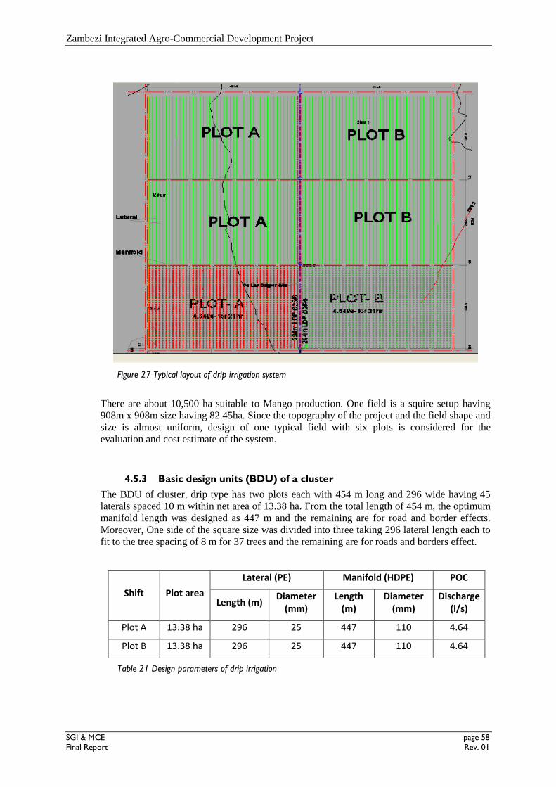
Zambezi Integrated Agro-Commercial Development Project
SGI & MCE page 58
Final Report Rev. 01
Figure 27 Typical layout of drip irrigation system
There are about 10,500 ha suitable to Mango production. One field is a squire setup having
908m x 908m size having 82.45ha. Since the topography of the project and the field shape and
size is almost uniform, design of one typical field with six plots is considered for the
evaluation and cost estimate of the system.
4.5.3 Basic design units (BDU) of a cluster
The BDU of cluster, drip type has two plots each with 454 m long and 296 wide having 45
laterals spaced 10 m within net area of 13.38 ha. From the total length of 454 m, the optimum
manifold length was designed as 447 m and the remaining are for road and border effects.
Moreover, One side of the square size was divided into three taking 296 lateral length each to
fit to the tree spacing of 8 m for 37 trees and the remaining are for roads and borders effect.
Shift Plot area
Lateral (PE) Manifold (HDPE) POC
Length (m) Diameter
(mm) Length
(m) Diameter
(mm) Discharge
(l/s)
Plot A 13.38 ha 296 25 447 110 4.64
Plot B 13.38 ha 296 25 447 110 4.64
Table 21 Design parameters of drip irrigation

Zambezi Integrated Agro-Commercial Development Project
SGI & MCE page 59
Final Report Rev. 01
As a sample, Basic Design Unit of a cluster selected two plots under one valve having filter,
pressure regulator, fertilizer injector and other fittings. These two plots will be operated by the
same operating unit and will be supplied each 4.64 l/s water parallel at time making the total
discharge at operating unit point of connection as .28 l/s. As the design of shifts is one, within
21hr three operation units having six plots each will be irrigated plot (Figure 28 and Figure
29).
Figure 28 Basic Design Unit of a Cluster, for fruit

Zambezi Integrated Agro-Commercial Development Project
SGI & MCE page 60
Final Report Rev. 01
Figure 29 Basic Design of one plot
4.5.4 Selection of drippers, type, spacing and discharge
For fruit trees, dripper type of on line dripper with smooth outlet of pressure compensating
type is selected because of attaining the discharge uniformity within the plot of the project
unit.
The discharge of an emitter is generally expressed by the power curve equation:
(equation 7)
where:
H = average emitter pressure head, (m)
q = average emitter discharge (1/hr)
x and k = coefficients that characterize a specific emitter.
Usually these are obtained or calculated from the manufactures catalogue or test results. The
expected uniformity of application shall be more than 90%. In this specific study, discharge is
taken from the manufacturers’ catalogue. Assuming that:
Plant tree is Mango tree, with recommended tree spacing of 10m by 8m;
One lateral per tree raw;
Selected dripper type is On-line dripper;
Drippers each apply 2 l/hr at minimum recommended operating pressure of 1 to 1.5
bar; (discharge pressure relationship from manufacturer’s standard )
Soil is sandy;
Dividing the determined crop water requirement of 212 litter/ day / plant to that of 21 hrs/day
irrigation times, 10 litres / hr discharge is to be applied for one plant. Hence, to meet the 10
lit/hr discharge requirement of one plant, 5 drippers are required with a dripper discharge of 2
l/hr.
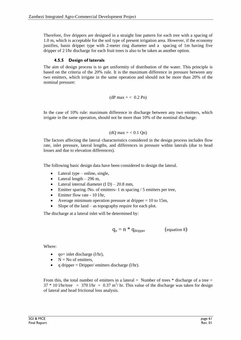
Zambezi Integrated Agro-Commercial Development Project
SGI & MCE page 61
Final Report Rev. 01
Therefore, five drippers are designed in a straight line pattern for each tree with a spacing of
1.0 m, which is acceptable for the soil type of present irrigation area. However, if the economy
justifies, basin dripper type with 2-meter ring diameter and a spacing of 1m having five
dripper of 2 l/hr discharge for each fruit trees is also to be taken as another option.
4.5.5 Design of laterals
The aim of design process is to get uniformity of distribution of the water. This principle is
based on the criteria of the 20% rule. It is the maximum difference in pressure between any
two emitters, which irrigate in the same operation and should not be more than 20% of the
nominal pressure:
(dP max = < 0.2 Pn)
In the case of 10% rule: maximum difference in discharge between any two emitters, which
irrigate in the same operation, should not be more than 10% of the nominal discharge:
(dQ max = < 0.1 Qn)
The factors affecting the lateral characteristics considered in the design process includes flow
rate, inlet pressure, lateral lengths, and differences in pressure within laterals (due to head
losses and due to elevation differences).
The following basic design data have been considered to design the lateral.
Lateral type – online, single,
Lateral length – 296 m,
Lateral internal diameter (I D) – 20.8 mm,
Emitter sparing /No. of emitters- 1 m spacing / 5 emitters per tree,
Emitter flow rate - 10 l/hr,
Average minimum operation pressure at dripper = 10 to 15m,
Slope of the land – as topography require for each plot.
The discharge at a lateral inlet will be determined by:
qo = n * qdripper (equation 8)
Where:
qo= inlet discharge (l/hr),
N = No of emitters,
q dripper = Dripper/ emitters discharge (l/hr).
From this, the total number of emitters in a lateral = Number of trees * discharge of a tree =
37 * 10 l/hr/tree = 370 l/hr = 0.37 m3/ hr. This value of the discharge was taken for design
of lateral and head frictional loss analysis.
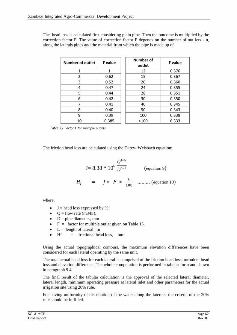
Zambezi Integrated Agro-Commercial Development Project
SGI & MCE page 62
Final Report Rev. 01
The head loss is calculated first considering plain pipe. Then the outcome is multiplied by the
correction factor F. The value of correction factor F depends on the number of out lets - n,
along the laterals pipes and the material from which the pipe is made up of.
Number of outlet F value
Number of outlet
F value
1 1 12 0.376
2 0.62 15 0.367
3 0.52 20 0.360
4 0.47 24 0.355
5 0.44 28 0.351
6 0.42 30 0.350
7 0.41 40 0.345
8 0.40 50 0.343
9 0.39 100 0.338
10 0.385 >100 0.333
Table 22 Factor F for multiple outlets
The friction head loss are calculated using the Darcy- Weisbach equation:
J= 8.38 * 106
75.4
75.1
D
Q
(equation 9)
......... (equation 10)
where:
J = head loss expressed by %;
Q = flow rate (m3/hr);
D = pipe diameter., mm
F = factor for multiple outlet given on Table 15.
L = length of lateral , m
Hf = frictional head loss, mm
Using the actual topographical contours, the maximum elevation differences have been
considered for each lateral operating by the same unit.
The total actual head loss for each lateral is comprised of the friction head loss, turbulent head
loss and elevation difference. The whole computation is performed in tabular form and shown
in paragraph 9.4.
The final result of the tabular calculation is the approval of the selected lateral diameter,
lateral length, minimum operating pressure at lateral inlet and other parameters for the actual
irrigation site using 20% rule.
For having uniformity of distribution of the water along the laterals, the criteria of the 20%
rule should be fulfilled.

Zambezi Integrated Agro-Commercial Development Project
SGI & MCE page 63
Final Report Rev. 01
In the present irrigation field case, the maximum pressure variation between two drippers in
the same plot area should be less than 20% of the nominal pressure at the outlet of the
operation unit.
In the lateral designs as shown in paragraph 9.4, computed and checked the fulfilment of the
20% rule, for all used lateral diameters and lengths.
During computation of each plot and lateral pressure variations, all the actual maximum
topography differences in each plots and entire the laterals and manifolds, head losses are
considered. The lateral inlet pressure was determined with equation 11.
........... (equation 11)
Where,
Hi = Lateral inlet pressure, m
Ho = Average operating pressure of dripper, nominal pressure, manufacturer’s
specifications, m
Hf = frictional head loss in the lateral, m
ΔZ = change in elevation in the lateral alignment, m
4.5.6 Design of manifolds
The discharge in each manifold is determined by:
qm= (qa * N) Nr........... (equation 12)
where:
qm = discharge in each manifold (l/hr)
qa = average emitter discharge (l/hr) =2
N = No. of dripper/ emitters in a lateral =185
Nr = No. of laterals in a manifold = 45
Using equation 12, the discharge on manifold = 2 X 185 X 45 = 16650 l/hr = 16.65 m3/hr
and this value was used to analyse the pressure and discharge in the manifold.
The frictional head loss in the inlet of the manifold was determined using equation 9 and
equation 10 and inlet pressure at the manifold is using equation 13.
........... (equation 13)
Where,
Hm = Manifold inlet pressure ,m
Hi = = Lateral inlet pressure, m
Hf = frictional head loss in the manifold, m
ΔZ = change in elevation in manifold alignment, m
The full analysis and results are presented in paragraph 9.4.
Two main requirements on manifold diameter determination are the following.

Zambezi Integrated Agro-Commercial Development Project
SGI & MCE page 64
Final Report Rev. 01
First of all, the manifold diameter should be economical. As discussed in the determination of
the delivery pipe diameter, the most precise method for determination of the economical
diameter is detail computation of the total cost of the pipe at different diameter sizes and select
diameter with the least total cost.
Here the total cost of different diameter pipes shall include cost of pipe (conduit) for the whole
length, cost of energy, which represent the head losses in the pipe diameter under
consideration, other installation, operation, and maintenance costs.
A second issue is that manifold should be quite enough strong against water hammer pressure,
which may occur due to sudden closure or sudden opening of valves (mainly at the manifold
inlet valve). For this reason, the velocity shall be limited bellow 1.5 to 2.0 m/sec.
The manifold diameter was determined by:
............... (equation 14)
where:
Qm = discharge in each manifold (l/hr)
V = Recommended velocity (m/sec)
D = Manifold internal diameter
Considering both requirements, the detail analysis of economical diameters, for the manifolds
pipes, at each plot is performed in paragraph 9.4.
4.6 MAINTENANCE OF IRRIGATION SYSTEMS
The purpose of an irrigation scheme is to achieve a higher crop production level through
appropriate management and planning of water distribution practices. This can be achieved
through better and organized project management practices.
Good operation of any irrigation system includes matching the irrigation duration with the rate
of application and the intake rate of the soil to maximize the fraction of water stored in the
root zone. If a field is under-irrigated, all the infiltrated water could be stored in the root zone,
giving apparently high irrigation efficiency even though the water distribution uniformity
across the field may be poor.
Conversely, an over-irrigated field will have low irrigation efficiency even if the irrigation
appears to be uniform, because of the deep percolation. Thus, knowledge of the soil moisture
content prior to irrigation is essential to maintaining high application efficiency while
providing sufficient water for optimum crop growth.
Proper maintenance involves anticipating the need for repairs and replacement of worn-out
mechanical parts and damaged or broken pipes. Spare parts of commonly needed items should
be kept on hand for emergencies. Periodic inspection of supply pipes, mechanical equipment
(such as pumps, nozzles, emitters and filters) and distribution systems should be made
throughout the irrigation season.
It is important to perform preventative maintenance in the fall, winter, and/or early spring in
order to be ready for the next irrigation season. An audit or evaluation of the irrigation system
is recommended if the system is not as efficient as it should be. An audit determines the depth
of water being applied and distribution uniformity. If a pump is used, it is tested to determine
fuel or energy use efficiency.

Zambezi Integrated Agro-Commercial Development Project
SGI & MCE page 65
Final Report Rev. 01
4.6.1 Sprinkler
Regular maintenance of sprinkler equipment will reduce repair costs, help the system last
longer, and keep irrigation efficiency at design levels. Each manufacturer provides guidelines
and manuals for equipment operation and maintenance. Such information is the preferred
source and should be referenced when performing irrigation equipment repair and
maintenance.
Sprinkler systems should be inspected and any necessary repairs completed prior to the start of
the irrigation season. All irrigation systems should receive special attention at the end of each
irrigation season. During the fall, while water is still available for operation, it is advisable to
run the sprinkler system and look for problems. This will allow to plan for any needed
maintenance well in advance of the next irrigation season. Check all nozzles for plugging,
mismatched sizes, breakage, corrosion or other damage caused by wear and tear. Couplers and
connections should be checked for leaks and repairs/replacements should be completed as
soon as possible.
If a sprinkler system has been properly prepared for winter storage, spring maintenance is
much easier. Often local irrigation supply companies provide a fall or winter tune-up service
at a reasonable cost. If the field is used for pasture, careful attention should be given to
protecting the irrigation system from livestock damage.
Sprinkler package selection is a major topic when making the original purchase of the center
pivot, but it is just the first decision related to managing the center pivot year-in, year-out. To
be effective, the
Sprinklers must continue to run properly which means that when wear and tear causes the
sprinkler to malfunction, repair or replacement is necessary. Once installed, it is more
important to ensure that each sprinkler continues to operate as it was designed.
Field topography and pumping plant performance can have major impacts on the performance
of a sprinkler package. Sprinklers may be damaged by a myriad of issues at any time after the
original installation. Failures to replace damaged sprinklers or remove materials that may plug
nozzle openings allow the water application to be affected in a negative manner for extended
periods. Keeping good records on pumping plant performance and performing a simple
sprinkler system check on a regular basis will help ensure that the system is operating
efficiently.
The design sprinkler flow rate out of each sprinkler orifice is based on the water pressure
supplied to the sprinkler inlet. Overall, the discharge delivered by a sprinkler also depends on
the system capacity, the distance from the pivot point to a specific sprinkler, and the spacing
between sprinklers at that location on the lateral. The goal of the sprinkler package selection
or design process is select nozzles that would apply water with over 90% application
uniformity.
The nozzle diameter has a big influence on the discharge from the nozzle since the discharge
depends on the square of the nozzle diameter. Depending on the construction material of the
nozzle and the quality of water being pumped, the nozzle opening could change. If the nozzle
opening increases due to wear, the actual flow rate may be vastly different than the original
design.
What are the problems associated with center pivot sprinkler operation?
The most obvious answer to this question is that over time various parts of the sprinkler can
become worn-out to the point where it no longer distributes water over the same wetted area in
a uniform manner. However, in some cases the original installation can be the issue.
It is always good to conduct the inspection just before sunrise and sunset as the angle of light
from the sun makes it easier to identify water application problems. Each sprinkler should be
Zambezi Integrated Agro-Commercial Development Project
SGI & MCE page 66
Final Report Rev. 01
operating and look very similar to the sprinkler next to it. If not, the regulator or nozzle
opening could be partially plugged.
Each of the issues described above could have been identified by a simple three-part
inspection, which is best done in the spring before the crop canopy is present:
1. Verify that the correct flow rate and operating pressure supplies the system,
2. Compare the sprinklers sizes installed to the sprinkler design printout,
3. Verify that the sprinkler is not cracked or broken and that the deflection pads are not
worn excessively.
Why is water application uniformity important?
The original sprinkler package design will normally have water application uniformity above
90% when operated under no wind conditions. Reduced water application uniformity means
that some areas of the field are not receiving the correct amount of water.
If any of the issues discussed above are present the non uniformity can occur each time water
is applied and the accumulative impact is that grain or forage yield can be less than expected.
Often times small problems that affect only a few sprinklers may not be noticeable in yield
maps while others can easily be seen from the air.
4.6.2 Drip
Flush the system at the beginning of the growing season and check to be sure the emitters are
not clogged. Do this by opening the ends of the tube and running clean water through the
system, starting with the lines closest to the supply source. Once the tubes have all been
checked and sealed again, check for flow from each emitter. Regular flushing of the system
throughout the season may be necessary depending on the cleanliness of the water supply and
filtering system. This will help remove larger mineral and organic matter particles that can
clog emitters. To keep the small openings in low-flow systems from becoming clogged, the
water source must be properly filtered. The cleanliness of the irrigation water will determine
how often the filters should be checked and cleaned. If continual clogging is a problem, it may
be necessary to select finer screens or use a sand filter or chemically treat the water.
4.6.3 Filters
Check the filters regularly and frequently until the best cleaning schedule for the system can
be determined. The frequency of cleaning the filters may be greater in the spring when more
debris is in the water. Back flushing, or removing the filters and washing them out backwards
is the most common way to clean most filters. Replace the filters when they get holes or
openings too large to filter out damaging or clogging particles. Organic matter slipping past
the filter or algae growing in pipes or fittings may cause serious system problems, especially
when the source is a secondary water system. Opening the end of the system and flushing will
help remove organic matter. If algae growth is a problem, chlorine can be used to kill the
algae. Applying a concentration of 10 to 20 ppm of chlorine for 30 to 60 minutes should solve
most algae problems. After the algae have been killed, it will need to be flushed as described
above.
Both screen and sand media filters in a drip irrigation system should be checked during or
after each operating period and cleaned if necessary. A clogged screen or grooved-disk filter
can be cleaned with a stiff bristle brush or by soaking in water. A sand media filter should be

Zambezi Integrated Agro-Commercial Development Project
SGI & MCE page 67
Final Report Rev. 01
back flushed when pressure gauges located at the inlet and outlet sides indicate a five psi
difference. Check drip irrigation lines for excessive leaking, and look for large wet areas in the
planting area indicating a leaking tube or defective emitter. It is also a good practice to flush
sub-mains and laterals periodically to remove sediments that could clog emitters. Systems can
be designed with automatic back flushing devices and automatic end line flushing devices, but
still require manual checks.
4.6.4 Chemical Control Measures
Unfortunately, filtration alone is not always adequate to solve all water quality problems.
Chemicals are necessary to control algae, iron and sulfur bacteria, and disease organisms.
Chemicals can cause some materials to settle out or precipitate out of the water while causing
other materials to maintain solubility or stay dissolved in the water. Chlorine is a primary
chemical used to kill microbial activity, to decompose organic materials, and to oxidize
soluble minerals, which causes them to precipitate out of solution. Acid treatments are used to
lower the water pH to either maintain solubility or to dissolve manganese, iron, and calcium
precipitates that clog emitters or orifices. Potassium permanganate also is used to oxidize iron
under some conditions. It is recommended to place the filtration system after the chemical
treatment to remove any particles formed. Chemigation protection and injection equipment
requirements vary with toxicity class of the injected chemicals.
4.6.5 Bacterial Slimes/Precipitates
Bacteria can grow in the absence of light within the system or in a contaminated reservoir.
The bacteria can live on iron or sulfur and produce a mass of slime that quickly clogs emitters
and filters. This slime can also act as an adhesive to bind other solids together to cause
clogging. They also can cause soluble iron and sulfur to precipitate out of the water.
Bacteria cause iron precipitation by oxidizing soluble ferrous oxide to form insoluble ferric
oxide. Iron concentrations as low as 0.1 ppm can be troublesome, whereas levels of 0.4 ppm
can be severe. The iron precipitate forms as a red filamentous sludge, which can attach to PVC
and polyethylene tubing and completely block emitters.
Sulfur in amounts over 0.1 ppm of total sulfides can be troublesome in irrigation water.
Bacteria that live on sulfur can produce white stringy masses of slime, which can completely
block the emitting devices. Interactions of soluble iron and sulfur can lead to a chemical
reaction forming insoluble iron sulfide. Stainless steel filter screens used in high sulfide water
can cause iron sulfide precipitation. Chlorination is the usual treatment to kill bacteria or
inhibit their activity. A continuous residual rate of 1 to 2 ppm of free available chlorine at the
distant end of the irrigation system or an intermittent rate of 10 to 20 ppm for 30 to 60 per
treatment cycle should be effective. The initial injection rate may need to be higher to achieve
the desired residual level in the system. Treatment cycles may be required at the end of each
irrigation cycle for severe water sources or after every 10-20 hours of irrigation for cleaner
water sources.
Sometimes, reservoirs are contaminated with bacteria and shock chlorination is necessary to
reduce or solve the problem. This is done by injecting chlorine at a rate of 200 to 500 ppm into
the reservoir. The volume of water to be treated must be estimated from the diameter and
depth of the reservoir.

Zambezi Integrated Agro-Commercial Development Project
SGI & MCE page 68
Final Report Rev. 01
4.6.6 Algae and Aquatic Plants
Algae and aquatic plants in surface waters can be great nuisances’ because they reproduce
rapidly during summertime blooms. They have a tendency to become entangled in screen
meshes and clog the surface of sand media filters, resulting in frequent filter back flushing.
Algae can be controlled in surface waters by adding copper sulfate or other chemicals in an
approved manner. Green algae can grow only in the presence of light, so they do not cause a
problem in buried pipelines or black polyethylene. However, algae can grow in the white PVC
pipe or fittings used to assemble aboveground pipelines and then be washed into laterals and
emitters to cause clogging. Chlorine is used to kill algae within the irrigation system. A
chlorine concentration of 10 to 20 ppm for between 30 and 60 minutes is suggested. It is
advisable to work section-by-section through the pipeline and flush the dead algae out of the
pipes immediately after treatment, to prevent emitters clogging. If significant emitter clogging
occurs, a higher concentration may be needed to decompose the organic matter in the emitter.
4.6.7 Chemical Precipitation of Iron
Water with over 0.1 ppm of iron is quite likely to cause a problem in irrigation systems. The
problem can be solved by either removing the iron from the water or by retaining the iron in
solution.
4.6.8 Chlorine precipitation
Free chlorine will instantly oxidize ferrous iron to ferric iron and take it out of solution as a
solid. The iron concentration must be determined, and chlorine must be injected at a rate of 1
ppm for each 0.7 ppm of iron. Some additional chlorine may be needed for other
contaminants, such as iron bacteria and bacterial slime. Complete mixing of the chlorine and
water is necessary and can be accomplished by creating turbulence in the system before the
filter. A sand media filter is the most appropriate choice and should be backwashed frequently,
preferably automatically.
If manganese is present in the water source, caution must be exercised, because oxidation of
manganese by chlorine occurs at a much lower rate. Care must be taken to precipitate the
manganese before the filter, or clogging problems could occur.
4.6.9 pH Control
Iron is more soluble at lower pH values. Acid can be continuously injected to keep the pH low
in the irrigation system or can be used periodically to dissolve iron deposits. To dissolve the
iron, the pH must be reduced to approximately 2.0 or less for a period of 30 to 60 minutes.
The system must be flushed to remove the iron after treatment.
Iron precipitation can be caused by raising the pH. A solution to increase the pH can be
prepared by mixing 3 pounds of soda ash (58 percent light grade) with 4 gallons of water. This
neutralizing solution can be injected into the water system and can be mixed with chlorine
solutions.
4.6.10 Iron Sulfide Precipitation
Sulfur-bearing minerals are common in most sedimentary rocks. A soluble form of sulfate is
carried by water. Sulfates are difficult to precipitate and generally remain in solution. Sulfate
can be used as a food source by bacteria, which produces hydrogen sulfide gas as a by-

Zambezi Integrated Agro-Commercial Development Project
SGI & MCE page 69
Final Report Rev. 01
product. If sufficient iron is present under moderate reducing conditions, iron sulfides can be
precipitated, and a sand media filter is suggested to remove the precipitate.
4.6.11 Precipitation of Calcium Salts
Calcium salts, particularly calcium carbonates, precipitate out as a white film or plating in the
system. The salts are soluble at low pH. Acid can be used to maintain a pH of 4.0 or lower for
30 to 60 minutes which dissolves calcium deposits to clean emitters and pipelines.
Hydrochloric (muriatic) acid is recommended for treating calcium blockages although sulfuric
and phosphoric acid can also be used. Temperature, pH, and calcium concentration are all
factors influencing calcium solubility, so conditions can vary throughout the irrigation system.
Water sources differ in the amount of hardness and/or pH requiring different amounts of acid
to lower the pH.
The most common acid that growers will find available is muriatic acid (20% hydrochloric
acid) at hardware and farm supply stores. Make sure that you flush and clean the injector after
acid application since the acid may be corrosive to internal parts. Allow the acid treated water
to remain in the pipe lines for 30 minute to 1 hour, and then flush with water. Use extreme
care in handling acids and always add acid to water.
In general, the maintenance of drip system centers on identification of the factors, which can
lead to reduction of the performance of drip system and procedures to mitigate these negative
impacts. Factors that can slow or stop flow through the drip system include; suspended
material, chemical precipitation, biological growth, root intrusion, soil ingestion and crimping
of the drip line. To ensure maximum system life reduces or eliminates the impact of the
negative factors (Table 1). This may require water treatment and a systematic program for
regular maintenance. In this section, we outline the various potential issues that can adversely
affect the drip system and offer procedures to mitigate the potential damage.
Indication Possible problem
Gradual decrease in flow rate Dripper plugging Possible pump wear
(check pressure)
Sudden decrease in flow rate Stuck control valve Water supply failure
Gradual increase in flow rate Incremental damage to dripper line by pests
Sudden increase in flow rate Broken lateral, manifold, secondary or
primary lines Pressure regulator failure
Large pressure drop across filters Debris buildup in filters Inadequate flushing
of filters
Gradual pressure decrease at filter
inlet
Pump wear or water supply problems
Sudden pressure decrease at filter
outlet
Broken lateral, manifold, secondary or
primary pipe line Pressure regulator or
water supply failure
Gradual pressure increase at filter
outlet
Dripper plugging
Sudden pressure increase at filter
outlet
Stuck control valve , Other flow restrictions
Sudden pressure decrease at manifold Damaged or broken lateral
Table 23 Drip induction and possible problems

Zambezi Integrated Agro-Commercial Development Project
SGI & MCE page 70
Final Report Rev. 01
4.7 REFERENCES FOR IRRIGATION SYSTEM DESIGN
Jack Keller and Ron D. Bliesner, 1990Sprinkle and Trickle Irrigation. An avi Book. Published by Van Nostrand Reinhold, New York
FAO (1998). Crop evapotranspiration: guidelines for computing crop water requirements, FAO Irrigation and Drainage Publications No 56, Rome.
G.Gupta, 2002. Drip Irrigation design and operation
TAHAL (2000), National Master Plan for Agricultural Development, Final Report
Vol I, Main Report,
Mid-Term Review of National Development Plan (NPD) 10, Ministry of Finance
and Development Planning, 2013
.

Zambezi Integrated Agro-Commercial Development Project
SGI & MCE page 71
Final Report Rev. 01
5 ON DEMAND PRESSURIZED PIPED IRRIGATION SYSTEM
5.1 INTRODUCTION
The present feasibility study for an irrigation project in Pandamatenga takes into account what
has been already designed in the “Preliminary Design Report on Utilization of the Water
Resources of the Chobe/Zambezi River” redacted by WRC in November 2013.
In this document the water transfer scheme (WTS), shown in Figure 30, has been described:
after the water withdrawal from Chobe River a series of pumping stations, reservoirs and
pipes are aligned for about 580 km in order to join the Botswana's North-South Carrier (NSC),
that supply drinking water to Gaborone. In particular, this project foresees:
abstraction of 495 million m3 of water per annum from the Chobe/Zambezi River
System at Kazungula in the Chobe District, Botswana;
requirement for about 345 million m3 of water per annum for agricultural purposes,
mainly for the present ZIACD project;
future water deficit in urban centres to be at least 100 million m3
per annum;
conveyance of 150 million m3 from the Pandamatenga Reservoir through inter alia
Nata, Francistown and Tonota to be discharged into the existing North - South Carrier
Water Project at Break Pressure Tank (BPT1) located at Moralane area near Selebi –
Phikwe.
Figure 30. The already designed Chobe – Zambesi water transfer scheme (“Preliminary Design Report on
Utilization of the Water Resources of the Chobe/Zambezi River” by WRC, 2013)
The present irrigation project, according to the above figure, takes water from reservoir R2,
that has capacity of 2.0 Mm³ and is supplied by a pipeline with diameter 2.7 m and design
discharge of about 23.3 m³/s.
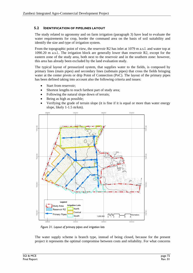
Zambezi Integrated Agro-Commercial Development Project
SGI & MCE page 72
Final Report Rev. 01
5.2 IDENTIFICATION OF PIPELINES LAYOUT
The study related to agronomy and on farm irrigation (paragraph 3) have lead to evaluate the
water requirements for crop, border the command area on the basis of soil suitability and
identify the size and type of irrigation system.
From the topographic point of view, the reservoir R2 has inlet at 1079 m a.s.l. and water top at
1090.20 m a.s.l.. The irrigation block are generally lower than reservoir R2, except for the
eastern zone of the study area, both next to the reservoir and in the southern zone: however,
this area has already been excluded by the land evaluation study.
The typical layout of pressurized system, that supplies water to the fields, is composed by
primary lines (main pipes) and secondary lines (submain pipes) that cross the fields bringing
water at the center pivots or drip Point of Connection (PoC). The layout of the primary pipes
has been defined taking into account also the following criteria and issues:
Start from reservoir;
Shortest lengths to reach farthest part of study area;
Following the natural slope down of terrain;
Being as high as possible;
Verifying the grade of terrain slope (it is fine if it is equal or more than water energy
slope, likely 1-1.5 m/km).
Figure 31. Layout of primary pipes and irrigation lots
The water supply scheme is branch type, instead of being closed, because for the present
project it represents the optimal compromise between costs and reliability. For what concerns

Zambezi Integrated Agro-Commercial Development Project
SGI & MCE page 73
Final Report Rev. 01
economic matter there are many facts that lead to money savings, while in terms of system
efficiency the main issue is that the agronomic study has envisaged an irrigation cycle of 4
days. This means that crops are watered during a day then there are 3 days of interval for the
next watering: during this period any local failure, that might occur, would be solved without
interfering with agricultural practises.
About costs, first of all, the branch type allows to reduce the length of the pipes to the lowest
value and also the required dimensions of the pipes are the smallest: this because each filed is
reached by only one primary system and there is no terminal portion of a pipeline system that
need to work also as an intermediate part of another one.
If this latter condition is considered, the loop pipeline could be designed either with a large
diameter, causing high cost of installation, or with small size, increasing energy expense and
requiring more powerful pumping system: this because head losses would be higher. Then
loop system need a larger number of cut-off valves.
The implementation of a closed network for the present irrigation system would need about 30
km of further pipes, beyond the 85 km that are currently envisaged. This would increase of a
third the present estimation of cost for primary pipes included in paragraph 5.3.2.
Finally, it has to be noted that the closed system is typical of the potable water supply where
consumers have to be constantly served even terms of water quantity but also for what
concerns pressure level. In case of agriculture, thanks to 4 days irrigation frequency and not
having the constrain of a continuous service, these limitations are not so strict.
Figure 32. Layout of secondary pipes and irrigation system (center pivot and drip)

Zambezi Integrated Agro-Commercial Development Project
SGI & MCE page 74
Final Report Rev. 01
The water transfer scheme, described in paragraph 5.1, would cross the irrigation area
interfering with infrastructures (irrigated fields, pipes, drains and roads) that are design with
the present project that is at feasibility level. Modification to the proposed layout in order to
avoid partially or totally interferences would neither affect the concept of the design, nor cause
significant variation in dimensioning and cost.
However, if the alignment is required, some fields would be reduced in extension and some
secondary pipe would be moved, but it would be worth to evaluate some minor changes even
for the track of WTS. Next figures represented the proposed alignment of center pivots,
secondary pipes and WTS.
Figure 33. Proposed alignment of center pivots, secondary pipes and WTS

Zambezi Integrated Agro-Commercial Development Project
SGI & MCE page 75
Final Report Rev. 01
Figure 34. Proposed alignment of center pivots, secondary pipes and WTS (details)
5.3 DESIGN OF PIPELINE NETWORK
5.3.1 General aspects and hydraulic criteria
There are several advantages in using pipelines for conveyance in water distribution projects
as well as for distribution on farm. A pressure pipeline system:
facilitates the use of flexible schedules because of the capacity to transmit pressure;
is an automated system for transmitting and carrying out precise instructions;
reduces considerably evaporation and seepage losses;
can be laid with straight alignments and go up and down hills because it do not have
to follow contours;
can convey water to higher elevation with the use of pumps and lifting plants;
reduces considerably required right-of way width in comparison with canals.
The selection of the type of pipe, diameters and materials must be done with great care in
order to insure that the initial installation is technically and economically acceptable and not
limiting for the future. This also because it is very difficult to make changes once pipelines
have been installed.
Besides, wrong type of pipe can cause an increase of the construction costs (transportation and
installation), a reduction of the system’s life, higher annual maintenance and power costs. The
diameter is a function of hydraulic issues, like flow rate and friction losses, that then affect
energy cost therefore the design is also the sizing of most economic pipe diameters.

Zambezi Integrated Agro-Commercial Development Project
SGI & MCE page 76
Final Report Rev. 01
Once that water requirements related to crops and pressure issue of irrigation system are set,
the design activities proceeds with the definition of the characteristics of a pipe that essentially
includes:
the material the pipe is made of;
the nominal diameter, which is the one considered for hydraulic calculation;
Hydraulically the material characterizes friction phenomenon through the roughness
coefficient, while the diameter determines the flow velocity: both of them are then related to
the head losses along the water supply system. These issue are described in the following
paragraphs (5.3.2 and 5.4).
5.3.2 Pipe materials
The selection of pipe materials consists in evaluating the characteristic of conveyed fluid and
soil where the pipe is supposed to be laid, but also the working conditions or rather the
external loads, such as seismicity, working pressure, transient conditions.
Other particular local conditions might be included in this analysis (for instance impervious or
densely inhabited areas), however it can be summarized that the water pipes should be
analyzed in term of:
mechanical resistance to internal and external loads;
resistance of physical, biological and chemical nature of conveyed water and soil;
flow resistance (smoothness) that must be the lowest possible;
ease and safety of installation;
comprehensive optimal cost, considering not only materials and installation but also
maintenance and duration.
A rough preliminary evaluation leads to identify small and medium diameters (less than 2000
mm) for the present irrigation system that is characterized by low pressure. In this field of
application, in general, pipes can be made of metallic, plastic or composites materials.
Anchoring
It is important to consider the possibility of leakage due to the soil movement and the
consequent joint disassembly due to soil settling as well as the effects of the internal pressure
that generate longitudinal forces on the pipeline. These forces have to be countered with
anchor blocks at vertices, branch offs, reductions and in the majority of cases where the
pipeline is tested hydraulically. The need to anchor the pipeline is reduced or does not exist
with the steel pipes since the continuity afforded by the welded joint makes them resistant to
the longitudinal forces.
Corrosion resistance
Metallic pipes are subject to corrosion both chemical in the ground and from the transported
fluid and also due to galvanic corrosion as opposed to GRP that is impervious to corrosion.
Corrosion control in steel pipes is made possible with internal and external coatings on the
pipes in the factory and during installation as well as during the life of the pipeline with
cathodic protection on the external surface. Cathodic protection requires continuous
monitoring and in certain areas is even subject to theft.
Resistance to Ageing
The only relevant analysis of the material behaviour is comparing the possible decay of their
characteristics with time and with working pressure . For water mains the analysis can be
restricted to pressure investigations as the temperature generally remains constant at around
20° C.

Zambezi Integrated Agro-Commercial Development Project
SGI & MCE page 77
Final Report Rev. 01
The behaviour of metallic materials and GRP are not influenced by the constant application of
the pressure forces. Plastic materials display a thermoplastic behaviour, while GRP is
designed with higher safety factors to account for ageing, but they are affected by pressure
surges that can cause vacuum in the pipeline if it is not protected from it.
Hydraulic characteristics
Steel pipes by virtue of modern manufacturing methods have considerably smooth surfaces.
The steel pipes with resin coating have an internal smoothness similar to that of GRP, at least
when new. Steel pipes with cement mortar lining have an absolute roughness greater than the
GRP pipes and this is important in as much as higher head losses: this has to be accounted for
at the design stage. GRP has a polished internal surface and therefore a very low absolute
roughness with benefits deriving from better flow, lower sedimentation and incrustation on the
internal surface.
Installation
Steel pipes are supplied in random lengths of around 10 m depending on the diameter that
determines the weight and therefore the weight limit of the site machinery. The progress is
hindered by the welding process and therefore (apart from the high investment in welding
equipment ) also the continuity of the internal and of the external protection must be restored.
Progress is 36 m/day in average.
GRP is lighter to install, does not require any protection, fittings are prefabricated and
installed without slowing down the installation, heavy equipment and service roads are not
required and with light equipment progress can be in the order of 120 m/day.
In the following table there is a comparison among the mentioned materials considering the
main issues related to a pressurized water supply system. It must be noted that given
judgments (for instance, lowest) are exclusively relative to the materials that are taken into
account, not in absolute.
MATERIAL &
PARAMETERS Steel
Polyvinyl
chloride
(PVC)
Glassfibre
Reinforced
Plastic (GRP)
Available sizes * any not for mains any
Laying & jointing
time &
experience
required
easy & fast easy & fast
Roughness low low lowest
Pressure resistance highest low low
Corrosion resistance prone ° resistant resistant
Maintenance periodical periodical not needed
Durability low lowest high
Basic cost costliest low lowest
Transport cost high low lowest
* Available sizes within the range needed for the present project
° Steel is prone to corrosion: mortar lining and cathodic protection are required
Table 24 Comparison among materials for pressured water supply networks
The most frequent method used to decide among various acceptable product alternatives is an
installed cost comparison. The results of such a restricted focus determination may be
misleading since, the installed cost evaluation ignores many other costs which may occur

Zambezi Integrated Agro-Commercial Development Project
SGI & MCE page 78
Final Report Rev. 01
during the lifetime of the pipelines. A reliable comparison must also consider the costs
incurred (or avoided) throughout the design life of the irrigation system.
The sum of all costs is called the Life Cycle Cost. This total cost of any item includes costs
experienced over the study period to:
purchase the item
install it
operate it
maintain & repair it
replace it (if necessary)
The pipe made by Glassfibre Reinforced Plastic (GRP) has the lowest life cost because they:
are durable and corrosion resistant
do not produce rust or scale suitable for potable water
are low in weight (¼ the weight of ductile iron and 1/10 th weight of concrete pipe)
require no cathodic protection
require no internal or external coatings
have flow efficiencies that allow down sizing
have a design life of 50 years
have zero maintenance costs
exhibit low internal friction, resulting into low operating (pumping) costs
show constant hydraulic characteristics over time
are suitable for high service pressures and temperatures
have easy and reliable jointing mechanisms
are suitable for underground and above ground applications
For all above, the Glassfibre Reinforced Plastic (GRP) might be suggested as the preferable
material for pipes for the current project.
5.4 IMPLEMENTATION OF COPAM MODEL FOR HYDRAULIC SIMULATION
The development process of an irrigation system follows a systematic chronological
sequence comprising the design, construction and management. Instead of seeing this as a
“one-way” process, it is important to think about it as an integrated process composed of
interrelated phases. The picture below presents key steps of an irrigation scheme development,
highlighting the parameters used in options identification and assessment.
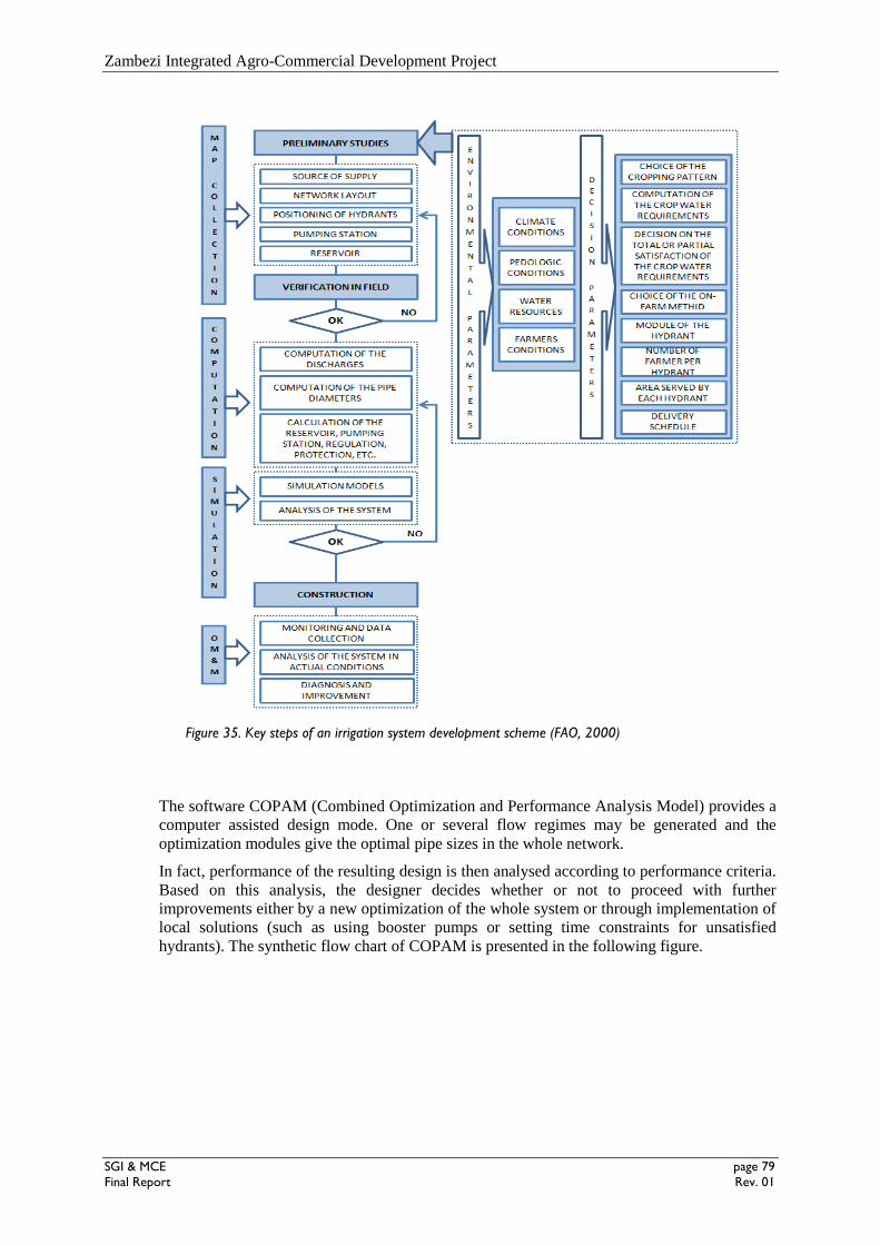
Zambezi Integrated Agro-Commercial Development Project
SGI & MCE page 79
Final Report Rev. 01
Figure 35. Key steps of an irrigation system development scheme (FAO, 2000)
The software COPAM (Combined Optimization and Performance Analysis Model) provides a
computer assisted design mode. One or several flow regimes may be generated and the
optimization modules give the optimal pipe sizes in the whole network.
In fact, performance of the resulting design is then analysed according to performance criteria.
Based on this analysis, the designer decides whether or not to proceed with further
improvements either by a new optimization of the whole system or through implementation of
local solutions (such as using booster pumps or setting time constraints for unsatisfied
hydrants). The synthetic flow chart of COPAM is presented in the following figure.

Zambezi Integrated Agro-Commercial Development Project
SGI & MCE page 80
Final Report Rev. 01
Figure 36. Synthetic flow chart of COPAM software (FAO, 2000)
5.4.1 Theoretical background
The discharges flowing into the network strongly vary over time depending on the cropping
pattern, meteorological conditions, on-farm irrigation efficiency and farmers' behaviour.
Because of this complexity, empirical methods give only general indications, while the
COPAM software implements statistical models aim to compute a single distribution of one or
more design flows for each pipe section of the network,
COPAM deals explicitly with calculation of pressurized irrigation systems capacity for on
demand operation thanks to a module that implements what has been studied by Clément
(1966). In particular, the “first Clément model” is based on a probabilistic approach where,
within a population of R hydrants, the number of hydrants being open simultaneously is
considered to follow a binomial distribution.
This model, although based on a theory, were extensively used for designing sprinkler
irrigation systems in France, Italy, Morocco and Tunisia. In fact, a probabilistic approach for
computing the discharges into the sections of an on-demand collective network has been
widely adopted because it is not reasonable to calculate the irrigation network by adding the
discharges delivered at all the hydrants simultaneously.
Considering hydrants with a different discharge, the total discharge downstream a generic
section k is given by:
2/12))1(()( jjj
j
jjj
j
j dPPRPqUdPRQ ;
R: number of hydrants downstream reach j;
P: probability of the hydrants downstream reach j to be open;
qs: specific continuous discharge (l/s/ha);
A: irrigated area (ha);
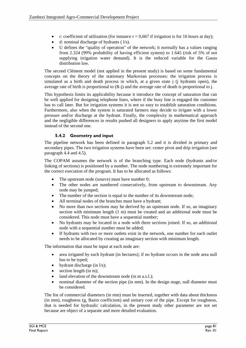
Zambezi Integrated Agro-Commercial Development Project
SGI & MCE page 81
Final Report Rev. 01
r: coefficient of utilization (for instance r = 0,667 if irrigation is for 16 hours at day);
d: nominal discharge of hydrants ( l/s).
U defines the "quality of operation" of the network; it normally has a values ranging
from 2.324 (99% probability of having efficient system) to 1.645 (risk of 5% of not
supplying irrigation water demand). It is the reduced variable for the Gauss
distribution law.
The second Clément model (not applied in the present study) is based on some fundamental
concepts on the theory of the stationary Markovian processes: the irrigation process is
simulated as a birth and death process in which, at a given state j (j hydrants open), the
average rate of birth is proportional to (R-j) and the average rate of death is proportional to j.
This hypothesis limits its applicability because it introduce the concept of saturation that can
be well applied for designing telephone lines, where if the busy line is engaged the customer
has to call later. But for irrigation systems it is not so easy to establish saturation conditions.
Furthermore, also when the system is saturated farmers may decide to irrigate with a lower
pressure and/or discharge at the hydrant. Finally, the complexity in mathematical approach
and the negligible differences in results pushed all designers to apply anytime the first model
instead of the second one.
5.4.2 Geometry and input
The pipeline network has been defined in paragraph 5.2 and it is divided in primary and
secondary pipes. The two irrigation systems have been set: center pivot and drip irrigation (see
paragraph 4.4 and 4.5).
The COPAM assumes the network is of the branching type. Each node (hydrants and/or
linking of sections) is positioned by a number. The node numbering is extremely important for
the correct execution of the program. It has to be allocated as follows:
The upstream node (source) must have number 0;
The other nodes are numbered consecutively, from upstream to downstream. Any
node may be jumped;
The number of the section is equal to the number of its downstream node;
All terminal nodes of the branches must have a hydrant;
No more than two sections may be derived by an upstream node. If so, an imaginary
section with minimum length (1 m) must be created and an additional node must be
considered. This node must have a sequential number;
No hydrants may be located in a node with three sections joined. If so, an additional
node with a sequential number must be added;
If hydrants with two or more outlets exist in the network, one number for each outlet
needs to be allocated by creating an imaginary section with minimum length.
The information that must be input at each node are:
area irrigated by each hydrant (in hectares); if no hydrant occurs in the node area null
has to be typed;
hydrant discharge (in l/s);
section length (in m);
land elevation of the downstream node (in m a.s.l.);
nominal diameter of the section pipe (in mm). In the design stage, null diameter must
be considered.
The list of commercial diameters (in mm) must be inserted, together with data about thickness
(in mm), roughness (g, Bazin coefficient) and unitary cost of the pipe. Except for roughness,
that is needed for hydraulic calculation, in the present study other parameter are not set
because are object of a separate and more detailed evaluation.

Zambezi Integrated Agro-Commercial Development Project
SGI & MCE page 82
Final Report Rev. 01
5.4.3 Simulation results
The program “Clément” allow the computation of the discharges flowing into the network
through the first and the second Clément models. In the present case the first one is selected,
and additional parameters have to be typed:
specific continuous discharge (in l/s/ha): this is according to the values included in
paragraph 4.4
minimum number of terminal open hydrants (5 is the chosen value)
percentage of uncultivated land (in %): in the present case this parameter is null;
Clément use coefficient (r) = 0.9167 because functioning is 22 hours a day;
Clément operation quality, U(Pq) = 1.654, that means 5% of failure.
On the basis of these assumptions, the simulation has given the following results: Table 25
indicates hydraulic characteristic of pipe in relation to the number of fields that are supplied,
while Table 26, Table 27 and Table 28 show the dimensioning in terms of diameter and head
losses along the primary pipes supplying the 3 irrigation lots.
Number of
supplied fields A (ha) Q (l/s) DN (mm) J (m/Km) V (m/s)
1 65 54 350 1.27 0.56
2 130 106 400 2.38 0.84
3 194 157 450 2.80 0.99
4 259 208 500 2.80 1.06
5 324 259 550 2.61 1.09
6 389 310 600 2.35 1.09
7 453 360 650 2.08 1.09
8 518 411 650 2.70 1.24
9 583 461 700 2.30 1.20
10 648 512 700 2.83 1.33
11 712 562 750 2.36 1.27
12 777 613 750 2.80 1.39
13 842 663 800 2.33 1.32
14 907 714 800 2.70 1.42
15 971 764 850 2.24 1.35
16 1,036 815 850 2.54 1.44
17 1,101 865 850 2.87 1.52
18 1,166 915 900 2.37 1.44
19 1,230 966 900 2.63 1.52
20 1,295 1,016 900 2.91 1.60
30 1,943 1,519 1,100 2.23 1.60
40 2,590 2,021 1,200 2.49 1.79
50 3,238 2,523 1,300 2.53 1.90
60 3,885 3,025 1,400 2.45 1.96
70 4,533 3,526 1,500 2.30 2.00
80 5,180 4,027 1,600 2.13 2.00
90 5,828 4,528 1,700 1.95 1.99
Zambezi Integrated Agro-Commercial Development Project
SGI & MCE page 83
Final Report Rev. 01
Number of
supplied fields A (ha) Q (l/s) DN (mm) J (m/Km) V (m/s)
100 6,475 5,029 1,800 1.77 1.98
110 7,123 5,530 1,900 1.60 1.95
120 7,770 6,030 2,000 1.45 1.92
130 8,418 6,531 2,100 1.31 1.89
140 9,065 7,031 2,200 1.19 1.85
150 9,713 7,532 2,200 1.36 1.98
Table 25 Hydraulic characteristic of pipe in relation with the number of fields that are supplied
Lot Reach Sub
Reach L (m) Field n° A (ha) Q (l/s)
DN
(mm) J (m/Km) V (m/s)
North
Reservoir R2 & Pumping Station
A 1 8345 112 7252 5630 1900 1.66 1.99
B
2 451 100 6475 5029 1800 1.77 1.98
3 915 93 6022 4678 1800 1.53 1.84
4 914 86 5569 4328 1700 1.78 1.91
5 914 79 5115 3977 1600 2.08 1.98
6 914 72 4662 3626 1600 1.73 1.80
7 914 64 4144 3225 1500 1.93 1.83
8 917 56 3626 2824 1400 2.13 1.83
9 914 48 3108 2423 1300 2.33 1.83
10 914 40 2590 2021 1200 2.49 1.79
11 911 32 2072 1620 1100 2.54 1.70
12 916 24 1554 1217 1000 2.39 1.55
13 914 16 1036 815 850 2.54 1.44
14 914 8 518 411 650 2.70 1.24
C 15 467 12 777 613 750 2.80 1.39
16 913 6 389 310 600 2.35 1.09
Table 26 Geometrical and hydraulic characteristics of primary pipes supplying North irrigation lot
Lot Reach Sub
Reach L (m) Field n° A (ha) Q (l/s)
DN
(mm) J (m/Km) V (m/s)
Central
Reservoir R2 & Pumping Station
A
1 541 142 9195 7131 2200 1.22 1.88
2 911 142 9195 7131 2200 1.22 1.88
3 915 137 8871 6881 2100 1.46 1.99
4 908 132 8547 6631 2100 1.35 1.91
5 902 124 8029 6231 2000 1.55 1.98
6 922 116 7511 5830 2000 1.36 1.86
7 923 108 6993 5430 1900 1.55 1.91
8 910 100 6475 5029 1800 1.77 1.98
9 444 93 6022 4678 1800 1.53 1.84

Zambezi Integrated Agro-Commercial Development Project
SGI & MCE page 84
Final Report Rev. 01
Lot Reach Sub
Reach L (m) Field n° A (ha) Q (l/s)
DN
(mm) J (m/Km) V (m/s)
B
10 4526 72 4662 3626 1600 1.73 1.80
11 915 63 4079 3175 1500 1.87 1.80
12 911 54 3497 2724 1300 2.95 2.05
13 913 48 3108 2423 1300 2.33 1.83
14 915 42 2720 2122 1200 2.74 1.88
15 914 36 2331 1820 1200 2.02 1.61
16 915 30 1943 1519 1100 2.23 1.60
17 914 24 1554 1217 1000 2.39 1.55
18 914 20 1295 1016 900 2.91 1.60
19 917 16 1036 815 850 2.54 1.44
20 915 12 777 613 750 2.80 1.39
21 889 7 453 360 650 2.08 1.09
22 937 2 130 106 400 2.38 0.84
C
23 452 15 971 764 850 2.24 1.35
24 917 14 907 714 800 2.70 1.42
25 915 12 777 613 750 2.80 1.39
26 917 9 583 461 700 2.30 1.20
27 914 5 324 259 550 2.61 1.09
Table 27 Geometrical and hydraulic characteristics of primary pipes supplying Central irrigation lot
Lot Reach Sub
Reach L (m) Field n° A (ha) Q (l/s)
DN
(mm) J (m/Km) V (m/s)
South
Reservoir R2 & Pumping Station
A
1 2638 145 9389 7282 2200 1.27 1.92
2 2838 45 2914 2272 1300 2.05 1.71
3 3967 8 518 411 650 2.70 1.24
4 814 7 453 360 650 2.08 1.09
5 816 4 259 208 500 2.80 1.06
B
6 540 100 6475 5029 1800 1.77 1.98
7 908 96 6216 4829 1800 1.63 1.90
8 914 93 6022 4678 1800 1.53 1.84
9 920 90 5828 4528 1700 1.95 1.99
10 911 88 5698 4428 1700 1.86 1.95
11 1523 87 5633 4378 1700 1.82 1.93
12 914 79 5115 3977 1600 2.08 1.98
13 914 71 4597 3576 1600 1.68 1.78
14 914 63 4079 3175 1500 1.87 1.80
15 914 55 3561 2774 1400 2.06 1.80
16 914 47 3043 2373 1300 2.24 1.79
17 914 39 2525 1971 1200 2.36 1.74
18 914 31 2007 1569 1100 2.38 1.65
19 914 23 1489 1167 1000 2.19 1.49
20 914 15 971 764 850 2.24 1.35
21 914 7 453 360 650 2.08 1.09
C 22 536 37 2396 1871 1200 2.13 1.65

Zambezi Integrated Agro-Commercial Development Project
SGI & MCE page 85
Final Report Rev. 01
Lot Reach Sub
Reach L (m) Field n° A (ha) Q (l/s)
DN
(mm) J (m/Km) V (m/s)
23 916 36 2331 1820 1200 2.02 1.61
24 1883 35 2266 1770 1100 3.03 1.86
25 914 30 1943 1519 1100 2.23 1.60
26 914 25 1619 1268 1000 2.59 1.61
27 914 20 1295 1016 900 2.91 1.60
28 914 15 971 764 850 2.24 1.35
29 914 10 648 512 700 2.83 1.33
30 914 6 389 310 600 2.35 1.09
31 914 3 194 157 450 2.80 0.99
32 914 1 65 54 350 1.27 0.56
Table 28 Geometrical and hydraulic characteristics of primary pipes supplying South irrigation lot
Figure 37. Supplied discharge along primary pipes for the study area

Zambezi Integrated Agro-Commercial Development Project
SGI & MCE page 86
Final Report Rev. 01
Figure 38. Diameter of primary pipes for the study area
5.4.4 Pumping system and power requirements
On the basis of simulation conducted with hydraulic model the head losses and the related
piezometry profile has been defined for each of the 3 irrigation system. Tables below indicate
the results of these computation.
Lot Reach Sub
Reach
Ground
Elevation
(m s.m.m.)
Piezometry
(m s.m.m.)
Pressure
Head (m)
Cumulated
Head Loss
(m)
North
Reservoir R2
& Pumping
Station
1081.00 1141 60 79
A 1 1070.06 1129 59 65
B
2 1069.91 1128 58 64
3 1069.17 1127 57 63
4 1068.00 1125 57 61
5 1068.00 1123 55 59
6 1067.99 1121 53 57
7 1067.86 1120 52 56
8 1067.39 1118 50 54

Zambezi Integrated Agro-Commercial Development Project
SGI & MCE page 87
Final Report Rev. 01
Lot Reach Sub
Reach
Ground
Elevation
(m s.m.m.)
Piezometry
(m s.m.m.)
Pressure
Head (m)
Cumulated
Head Loss
(m)
9 1066.16 1116 49 52
10 1065.62 1113 48 49
11 1065.02 1111 46 47
12 1064.03 1109 45 45
13 1063.43 1106 43 42
14 1062.55 1104 41 40
C 15 1070.06 1113 43 42
16 1070.94 1111 40 40
* Data are referred to the downstream node of indicated sub reach
Table 29 Head loss and piezometry for primary pipes supplying North irrigation lot
Lot Reach Sub
Reach
Ground
Elevation
(m s.m.m.)
Piezometry
(m s.m.m.)
Pressure
Head (m)
Cumulated
Head Loss
(m)
Central
Reservoir R2
& Pumping
Station
1081.00 1129 48 85
A
1 1080.39 1129 48 85
2 1078.81 1127 49 83
3 1076.15 1126 50 82
4 1073.03 1125 52 81
5 1070.19 1124 53 80
6 1067.31 1122 55 78
7 1065.54 1121 55 77
8 1063.41 1119 56 75
9 1062.51 1119 56 75
B
10 1059.44 1111 51 67
11 1057.85 1109 51 65
12 1056.00 1106 50 62
13 1055.06 1104 49 60
14 1054.00 1102 48 58
15 1052.81 1100 47 56
16 1052.00 1098 46 54
17 1050.00 1096 46 52
18 1049.00 1093 44 49
19 1047.52 1091 43 47
20 1046.44 1088 42 44
21 1045.49 1086 41 42
22 1044.00 1084 40 40
C
23 1062.70 1114 51 50
24 1063.01 1111 48 47
25 1064.00 1108 44 44
26 1064.00 1106 42 42
27 1064.00 1104 40 40
* Data are referred to the downstream node of indicated sub reach
Table 30 Head loss and piezometry for primary pipes supplying Central irrigation lot

Zambezi Integrated Agro-Commercial Development Project
SGI & MCE page 88
Final Report Rev. 01
Lot Reach Sub
Reach
Ground
Elevation
(m s.m.m.)
Piezometry
(m s.m.m.)
Pressure
Head (m)
Cumulated
Head Loss
(m)
South
Reservoir R2
& Pumping
Station
1081.00 1131 50 75
A
1 1078.85 1127 49 72
2 1071.15 1122 50 66
3 1066.00 1107 41 44
4 1064.00 1106 42 42
5 1063.41 1103 40 40
B
6 1078.00 1117 39 68
7 1075.63 1115 40 67
8 1074.18 1114 40 66
9 1072.71 1112 39 64
10 1070.37 1110 40 62
11 1066.84 1107 41 59
12 1065.92 1106 40 57
13 1063.36 1104 41 56
14 1061.36 1102 41 54
15 1059.00 1100 41 52
16 1058.45 1098 40 50
17 1056.29 1096 40 48
18 1054.55 1094 40 46
19 1053.00 1092 39 44
20 1050.56 1090 39 42
21 1048.13 1088 40 40
C
22 1071.00 1120 49 65
23 1070.63 1119 48 63
24 1068.83 1113 44 58
25 1067.30 1111 44 56
26 1066.86 1109 42 53
27 1063.35 1106 42 50
28 1061.00 1104 43 48
29 1060.45 1101 41 46
30 1059.00 1099 40 44
31 1056.45 1097 40 41
32 1055.35 1095 40 40
Table 31 Head loss and piezometry for primary pipes supplying South irrigation lot
It must be underlined that along the secondary pipe, serving generally about 5 fields, the head
losses are about 10 m, while at the centre pivot at least 30 m of residual pressure must be
guarantee, when the scenario with maximum water requirement is simulated. For this reason,
in the previous table, each of the 3 irrigation system has a final sub reach where the
“cumulated head loss” is 40 m (10 m plus 30 m ) or rather the “pressure head” is 40 m.

Zambezi Integrated Agro-Commercial Development Project
SGI & MCE page 89
Final Report Rev. 01
Figure 39. Piezometry along primary pipes for the study area
From this hydraulic computation, considering the reservoir has a bottom at 1081 m s.m.m., the
North, Central and South lots need a pumping system with the following characteristics.
Lot Discharge
(l/s) Head (m)
North 5630 60
Central 7131 48
South 7282 50
Table 32 Main characteristics of the 3 pumping system for the irrigation lots
According to the mentioned characteristics of pumping station, the power requirement is about
12,5 MW, while the annual energy consumption is around 64 million kWh/y.

Zambezi Integrated Agro-Commercial Development Project
SGI & MCE page 90
Final Report Rev. 01
Table 33 Plan of pumping system

Zambezi Integrated Agro-Commercial Development Project
SGI & MCE page 91
Final Report Rev. 01
Table 34 Cross section of pumping system

Zambezi Integrated Agro-Commercial Development Project
SGI & MCE page 92
Final Report Rev. 01
6 DRAINAGE SYSTEM AND ROADS
6.1 INTRODUCTION
The presence of irrigation agricultural practise (paragraph 3) and water supply network
(paragraph 5) leads to realize access roads and a drainage systems in order to collect storm
water falling within the fields and discharge it outside the study area, preventing that
infrastructures would be flooded.
The design of this drainage system starts from statistical analysis of rainfall included in
paragraph 2.4 and is based upon the estimation of storm water runoff (paragraph 6.3), but it
takes also into account what has been already envisaged for the neighbouring rainfed farms
(“Consultancy Services for Construction Supervision of Road Network and Drainage Systems
for Pandamatenga Farms – Final Design” by DIWI, October 2011).
In fact, according to this project there are several drains discharging water into the present
study area for an overall amount of about 170 m³/s for storm event with a return time of 10
years.
Figure 40. General layout of drainage system and access roads for existing farms (“Consultancy Services
for Construction Supervision of Road Network and Drainage Systems for Pandamatenga Farms – Final
Design” by DIWI in 2011)
6.2 IDENTIFICATION OF DRAIN AND ROAD LAYOUT
The layout of the water supply system for irrigation has been already described in paragraph
5.2: this pipeline network take also into account as well as the topography of the study area,
trying to follow the natural drainage paths.

Zambezi Integrated Agro-Commercial Development Project
SGI & MCE page 93
Final Report Rev. 01
This is obviously also the main criteria to set up the layout to collect and discharge storm
water that falls within the study area. The roads must simply guarantee access to each fields.
Besides, the drainage system has to intercept the runoff from adjacent zones and convey it to
the study area: naturally (northern border, see Figure 42) or artificially (drains for the existing
Pandamatenga farms, see Figure 40).
As for the pressurized pipeline network, also the storm water system is composed of primary
and secondary channels: these latter collect water directly from fields and discharge it into the
primary channels that generally are along the main natural drainage paths. Methodological
approach and numerical elaboration to dimension this channelization are given in paragraph
6.3 and 6.4.
Figure 41. Layout of primary drains for the present design and drainage system of the existing farms
The drainage system has to guarantee the safety of roads, especially at their intersection, but it
also must minimize risk related to sediment transport and wildlife. For these reasons, some
considerations for drain management are given in paragraph 6.6.
Zambezi Integrated Agro-Commercial Development Project
SGI & MCE page 94
Final Report Rev. 01
6.3 ESTIMATION OF STORM WATER RUNOFF
6.3.1 Identification of watersheds
The calculation of runoff starts from delineation and characterization of the watersheds that
are within the study area: first of all, these zones must be identified according to the drain and
road layout (paragraph 6.2), then they can be geometrically described.
For the primary drainage system the following image defines the watersheds whose
geometrical characteristics are extracted from the Digital Elevation Model (DEM) that has
been implemented during the present feasibility study, combining information from acquired
high resolution stereo pair images (with 50 cm of pixel dimension) and results of ad hoc
topographic field survey (more details in the Field Investigation Report).
Figure 42. Main watersheds of drainage system
As mentioned earlier, the secondary channels collect water directly from field therefore the
evaluation of their watershed takes into account the number of fields that they drain.
According to the definition of irrigation system, each field is a square with sides of 908 m thus
the total extension is 82.4 ha.

Zambezi Integrated Agro-Commercial Development Project
SGI & MCE page 95
Final Report Rev. 01
Figure 43. Layout of primary and secondary drains for the present design and drainage system of the
existing farms
The following image indicates the schematic draining system for fields: according to the
irrigation layout, the secondary channel might drain from 1 to maximum 5 fields.
The geometrical characteristics of watersheds related to primary and secondary drains are
summarized in Table 35 and Table 36.

Zambezi Integrated Agro-Commercial Development Project
SGI & MCE page 96
Final Report Rev. 01
Figure 44. Schematic layout of drainage system for fields towards the secondary drains
6.3.2 Time of concentration
The catchments are finally characterized from the hydrological point of view by the time of
concentration (tc) that measures the response of a watershed to a rain event. Generally the
procedures used to estimate tc depend upon few watershed characteristics. To accurately
determine tc for a watershed, the hydraulics of each part (overland and channel) of the flow
path can be distinguished. In some cases the two flow path can be taken into account in the
same formula or the computation can be done separately.
This parameter can be estimated with several formulas that are generally valid for a certain
extension of catchment. The formula from Aronica – Paltrinieri (1954) is applied when the
watersheds are smaller than 170 km² and it is derived from Giandotti’s formula (1934).
5.0
0
5.0
)(8.0
5.14
hh
LAt
m
c
(Giandotti, 1934)
5.0
0 )(8.0
5.11
hh
LAMdt
m
c
(Aronica e Paltrinieri, 1954)

Zambezi Integrated Agro-Commercial Development Project
SGI & MCE page 97
Final Report Rev. 01
Symbols included in formulas mean:
tc = time of concentration (hour);
A = basin area (km²);
L = flow path (km);
hm = sub-basin average elevation (m a.s.l.);
h0 = sub-basin lowest elevation (m a.s.l.);
M = coefficient related to vegetation coverage (ranging from 0.667 if bared to 0.167
when permanent grass);
d = coefficient related to soil permeability (ranging from 1.27 if semi impervious to
0.69 when high permeable).
The chosen values for coefficient M and d are respectively 0.2 (partially cultivated area) and
0.9 (moderately permeable soil). The geometrical characteristics of watersheds and the related
time of concentration are summarized in the following tables.
As regards the secondary channel, the watersheds have been related to the number of drained
fields as represented in Figure 44. On average drainage slope of fields (i) is about 1 m/km,
minimum elevation is factitiously set equal 0 and mean and maximum elevation is calculated
considering the diagonal length of field.
The following table indicates the concentration time in case of channels that drain from 1 to 5
fields. Calculation of concentration time for primary drain is referenced to basin drawn in
Figure 42.
Drained
fields
Area
(km²) L (km) H*min (m) H*avg (m) H*max (m) i (m/m) Tc (h)
1 0.82 1.3 0 0.6 1.3 0.0010 9
2 1.65 2.0 0 1.0 2.0 0.0010 11
3 2.47 2.9 0 1.4 2.9 0.0010 12
4 3.30 3.7 0 1.9 3.7 0.0010 13
5 4.12 4.6 0 2.3 4.6 0.0010 13
Table 35 Time of concentration for watersheds drained by secondary channels
Basin Area
(km²) L (km)
Hmin
(m a.s.l.)
Havg
(m a.s.l.)
Hmax
(m a.s.l.) i (m/m) Tc (h)
North 98 20.0 1062 1071 1080 0.0009 31
B1 58 18.1 1061 1067 1072 0.0006 33
B2 45 13.8 1061 1066 1070 0.0007 30
B3 4 2.1 1070 1073 1075 0.0024 9
A1 33 7.7 1064 1072 1080 0.0021 16
A2 17 5.7 1066 1073 1080 0.0025 13
A3 12 2.5 1061 1063 1064 0.0012 20
A4 9 3.6 1069 1073 1076 0.0020 13
C1 46 12.8 1043 1052 1060 0.0013 21
C2 45 12.8 1043 1052 1060 0.0013 21
D1 39 10.1 1048 1057 1066 0.0018 18
Zambezi Integrated Agro-Commercial Development Project
SGI & MCE page 98
Final Report Rev. 01
Basin Area
(km²) L (km)
Hmin
(m a.s.l.)
Havg
(m a.s.l.)
Hmax
(m a.s.l.) i (m/m) Tc (h)
D2 34 10.1 1048 1057 1066 0.0018 17
E1 3 2.2 1068 1070 1071 0.0014 12
E2 34 8.9 1055 1062 1068 0.0015 19
F1 24 9.3 1080 1088 1095 0.0016 16
F2 35 9.3 1080 1088 1095 0.0016 18
Table 36 Time of concentration for watersheds drained by primary channels
6.3.3 Spatial analysis of rainfall
After having statistically analyzed the frequency of rainfall (paragraph 2.4), it is necessary to
evaluate their spatial variability. In fact, the reduction of the precipitation depth from a design
storm for a punctual to an effective (mean) depth over the entire watershed is essential in order
to not overestimate the volume of precipitation and to fit the design of hydraulic structures as
correct as possible.
Generically, this evaluation has been conducted introducing a parameter: the Areal Reduction
Factor (ARF) is defined as the ratio between the average areal depth of precipitation and the
average point depth. It ranges from 0 to 1 and is a function of storm characteristics (intensity
and duration), as well as basin characteristics (size, shape and geographic location).
The National Weather Service of the National Oceanic and Atmospheric Administration
(NOAA) has suggested a relationship to estimate the reduction of punctual rainfall (Figure 45)
according the extension of the catchment and the duration of storm event (Technical Report
NWS 24, “A Methodology for Point-to-Area Rainfall Frequency Ratios”).
This type of relationship has been also included in the Botswana Road Design Manual,
provided by Department of Roads , with reference to the intensity of precipitation (Figure 46):
this means taking into account also the time of return of storm event.
Figure 45 ARF related to storm duration and catchment area (Technical Report NWS 24, NOAA)
Zambezi Integrated Agro-Commercial Development Project
SGI & MCE page 99
Final Report Rev. 01
Figure 46 ARF related to rainfall intensity and catchment area (Botswana Road Design Manual)
The extension of the watershed included within study area is generally smaller than 50 km²,
the critical storm durations (time of concentration) are often longer than 12 hours and the
intensity of rainfall is lower than 10 mm/h, therefore the ARF is always close to 1.
However, in the present analysis the formulation proposed by U.S. Geological Survey has
been adopted:
)0386.01.1exp()1.1exp(1 25.025.0 AddARF
d = duration of storm event (hour);
A = basin area (km²).
The resulting ARF for each watersheds are been quoted in Table 39 and Table 40.
Zambezi Integrated Agro-Commercial Development Project
SGI & MCE page 100
Final Report Rev. 01
6.3.4 Runoff peak and hydrograph
The runoff is the result of the movement of rainfall excess over the watershed surface to its
outlet. This calculation is generally done applying a deterministic hydrological model that
allow the runoff generation to be evaluated: the precipitation event is first described in terms
of total volume, time and area of distribution. Losses, consisting of interception and
infiltration, are simulated and subtracted from the precipitation, resulting in direct runoff or
rainfall excess. Direct runoff is transformed into a direct runoff hydrograph usually by unit
hydrograph methods.
The runoff hydrograph is expression of a flow rate at a certain point of drainage network over
time: synthetic hydrographs are predictions based on watershed characteristics and assumed
rainfall intensities: the shape of a runoff hydrograph can be specified by the time to peak flow
and time for recession flow.
Among the procedures that are proposed in the technical literature to calculate the hydrograph
runoff, the Soil Conservation Service (U.S. Department of Agriculture, 1986) specifies a
triangular shape obtained using the so called rational formula (Wanielista, 1990). According to
this method, hydrograph time base (tb) and peak discharge (Qp) might be calculated as:
KCiAQp ; ppb xttt
where:
K = peak attenuation factor (see Table 37);
C = runoff coefficient;
I = average intensity of rainfall;
A = watershed area;
tp = time to peak, associated to time of concentration (see paragraph 6.3.2);
x = (1291/K) - 1 , if A is measured in square miles.
Table 37 Hydrograph attenuation factor (Wanielista, Yousef “Stormwater Management”, 1993)
Figure 47 Triangular shaped hydrograph related to hydrograph peak reduction factor included in Table 37
(Wanielista, Yousef “Stormwater Management”, 1993)

Zambezi Integrated Agro-Commercial Development Project
SGI & MCE page 101
Final Report Rev. 01
Table 38 Run-off coefficients for use in rational and modified rational methods (“Hydrological and
Hydraulic Guidelines, New Zeland”, 2012)
According to the data included in the previous tables and figure, the present study has adopted
conservatively 0.4 as runoff coefficient (cultivated soil), while the chosen peak attenuation
factor is the typical SCS (K = 484, x = 1,67): this is because the rational method (K = 645, x =
1) would probably overestimates the peak discharge.
The following tables include calculation related to SCS hydrograph runoff (Wanielista, 1990)
for secondary and primary drains on the basis of watersheds identified in Table 35 and Table
36. The storm event that has been considered has a return time of 10 years.

Zambezi Integrated Agro-Commercial Development Project
SGI & MCE page 102
Final Report Rev. 01
Drained
fields
Area
(km²) tc (h) tb (h)
Rainfall
intensity
(mm/h)
ARF Q (m³/s) u
(m³/s/km²) V (Mm³)
1 0.82 9.3 60.5 10.2 1.00 1.0 1.26 0.03
2 1.6 10.9 70.6 8.7 1.00 1.8 1.08 0.06
3 2.5 11.8 76.6 8.0 1.00 2.5 0.99 0.09
4 3.3 12.5 81.3 7.5 1.00 3.1 0.93 0.12
5 4.1 13.1 85.3 7.2 1.00 3.7 0.89 0.16
Table 39 Runoff hydrograph with 10 years return time for watersheds drained by secondary drains
Basin Area
(km²) tc (h) tb (h)
Rainfall
intensity
(mm/h)
ARF Q (m³/s) u
(m³/s/km²) V (Mm³)
North 98 31 200 3.4 0.97 40 0.41 4.0
B1 58 33 211 3.2 0.98 23 0.39 2.4
B2 45 30 194 3.5 0.99 19 0.43 1.9
B3 4 9 60 11.1 1.00 5 1.37 0.1
A1 33 16 107 6.2 0.98 25 0.76 1.3
A2 17 13 83 8.0 0.99 17 0.98 0.7
A3 12 20 127 5.4 1.00 8 0.66 0.5
A4 9 13 82 8.0 1.00 9 0.99 0.4
C1 46 21 137 5.0 0.99 28 0.61 1.9
C2 45 21 136 5.0 0.99 27 0.61 1.8
D1 39 18 117 5.8 0.99 28 0.72 1.6
D2 34 17 111 6.1 0.99 25 0.75 1.4
E1 3 12 75 8.8 1.00 4 1.09 0.1
E2 34 19 125 5.4 0.99 23 0.67 1.4
F1 24 16 106 6.2 0.99 18 0.76 1.0
F2 35 18 120 5.7 0.99 25 0.70 1.5
Total 537 - - - - - - 22
Table 40 Runoff hydrograph with 10 years return time for watersheds drained by primary drains
As mentioned in paragraph 6.1, there are some existing channels discharging water towards
the present study area; in particular some of them would interferes with the irrigation fields:
those are listed in the following table.
Because for these existing drains only the peak discharges are known, the storm water volume
is roughly estimated taking into account the ratio between volume (V) and peak discharge (Q)
that has been found for watershed within the study area (Table 43). On average this value is
about 20 hours.

Zambezi Integrated Agro-Commercial Development Project
SGI & MCE page 103
Final Report Rev. 01
Existing
drain code Q (m³/s) V (Mm³)
PD11 16.8 1.2
PD12 15.9 1.1
PD13 26.4 1.9
PD19 43.3 3.1
PD20 23.3 1.7
Total 126 9
As above indicated, the overall storm water volume for a 10-years event is about 31 Mm³ from
which 18 Mm³ are generated within the study area, 4 Mm³ from the outside northern basin and
9 Mm³ are brought by drains collecting water in neighbouring existing farms.
6.4 DESIGN OF GRAVITY DRAINAGE SYSTEM
The channels are designed to collect storm water falling within the fields and drain it outside
the study area. This system will allow agricultural practise and related infrastructure -
including roads and their intersection with channels (bridge and culvert), which are a critical
issue from a hydraulic point of view - to be preserved from floods. representing the most.
6.4.1 Design criteria
The dimensioning of the drainage system must make reference to different issues that are
analyzed within the present paragraph.
Time of return and freeboard.
First of all, the design must consider the probability of having a storm event that exceeds the
capacity of the drainage system and, therefore, causes floods within the study area. Obviously
the higher the chosen time of return, the greater will be the cost of realization.
The selection of this frequency of failure consists in a sort of risk assessment that is generally
related to the importance of the infrastructure to be protected. Typically national and
international standards suggest and/or prescribe certain return time but also, in some cases,
also the safety margin to be considered.
In fact, the freeboard between the water level (during the design storm event) and the top of
bank drain is normally governed by considerations about the channel itself (size, velocity,
etc...) but also about the risk of flood (importance of the surrounding property, structures,
etc...). Return period and freeboards that might adopted according to the traffic volume and
type of roads are indicated in the following table.
Road type Bridge standard Culvert standard
Major road
Passage of the 100-year return
period flood with minimum
clearance of 0.6 m normally
but with up to 1.2 m where
large trees can be transported
in the river.
− Passage of the 100-year return
period flood by heading up to a
maximum 0.5 m below road and
adjacent house floor levels, and
− Passage of the 10-year flood
without heading up.
Zambezi Integrated Agro-Commercial Development Project
SGI & MCE page 104
Final Report Rev. 01
Road type Bridge standard Culvert standard
Rural road
Passage of the 50-year return
period flood with a minimum
clearance of 0.6 m
− Passage of the 50-year return
period flood by overtopping the
embankment to a maximum
depth of 0.2 m, and
− Passage of the two year return
period flood with no heading up
Remote road
Passage of the 20-year return
period flood with a minimum
clearance of 0.3 m.
− Passage of the 20-year return
flood with 0.3 m freeboard, and
− Passage of the two year return
period flood with no heading up.
Access tracks
Passage of the 10-year return
period flood with a minimum
clearance of 0.3 m.
− Passage of the 10-year return
period flood by heading up to a
maximum 0.3 m below road
level.
Table 41 Time return and minimum freeboard for bridge and culvert according to road type
(“Hydrological and Hydraulic Guidelines, New Zeland”, 2012)
For the present project it has been adopted to make reference to flood event with 10-year
return and guarantee at least 50 cm as freeboard: this safety margin is also to prevent potential
reduction of geometrical cross section of the channel because of sediment deposition.
Material.
Fields survey and analogous experiences, as the agricultural zone next to the study area,
suggest to design unlined canal for the drainage network. This is mainly because eventual
seepage losses are not affecting the functioning of irrigation system, while concrete structures
would be costly for both construction and maintenance.
Therefore open channel will be excavated and shaped to the required cross section in natural
earth or filled without special treatment of the wetted surface. Compaction of bank or fill
material for the purpose of stabilization is not considered as a lining operation.
Geometry of cross section.
The trapezoidal cross section can be adopted for the primary and infield drains, primarily
because it is the simplest way to construct.
As flow is a function of cross sectional area the less the drain depth the greater the drain width
will need to be. The cross section selected for a canal should be such as to carry the design
storm discharge.
The ratio of bottom width to depth usually ranges from 2 : 1 for small channels to 6 : 1 for the
bigger drain, the side slopes of a canal depend upon the stability of the material in which it is
constructed. Inside slopes of 2 : 1 (horizontal to vertical) are practically standard for earth
canals under ordinary conditions.

Zambezi Integrated Agro-Commercial Development Project
SGI & MCE page 105
Final Report Rev. 01
Longitudinal slope and flow velocities.
The slope of the primary and infield drains is chosen according to the natural ground slopes
but also operation and maintenance problems should be considered in the selection of canal
cross-section characteristics.
This issue is mainly related to suggested values of flow velocity. In unlined canals, the
velocity should be such as to prevent erosion of the canal bottom (maximum allowable) or
deposition of soil that might be transported with water flow over fields (minimum allowable).
When the velocity of the flow is such that there is no silting or scouring action in the canal
bed, then that velocity is known as critical velocity. Generally the critical velocity depends on
the nature of the soil formation in which the water flows. Values of flow velocity that are
commonly suggested are from 0.3 to 0.6 m/s for sandy soil, 0.6 - 0.9 m/s for black cotton soil
and 0.9 to 1.15 m/s for firm clay and loom.
For what concerns the capacity of moving sediment downstream along the channels, the
evaluation can be done considering the formulation proposed by Shields that relates flow
dynamics to mean diameter of sediment (see paragraph 6.6.2).
6.4.2 Hydraulic dimensioning of primary and secondary drains
On the basis of all above mentioned criteria and the storm discharges resulting from
hydrological analysis (Table 39 and Table 40), the drainage system has been hydraulically
designed according to Manning’s formula, that allows to calculate flow capacity of channels
once that their geometrical and roughness characteristics are fixed:
AiRn
AVQ H 2/13/21
where:
Q = flowing discharge;
V = water velocity;
A = area of the cross section;
n = roughness coefficient (Manning’s number);
i = longitudinal slope;
RH = hydraulic radius, ratio between area and wetted perimeter.
Roughness is related to the material and condition of channel bottom and slopes: drain are
excavated, thus earth made, generally straight and with uniform cross section. According to
Chow, V. T. (Open Channel Hydraulics, 1959) value of Manning’s coefficient might be 0.022
if clean surface and 0.027 when short grass grows along the channel: for design purpose it has
been chosen the mean between the mentioned values (0.025).
The longitudinal slope is chosen according to the natural topography of the terrain where the
channel have been tracked. For what concerns the secondary drains, it has been considered
they have a common longitudinal slope of 0.5 m/km.
The cross section of drain is trapezoidal with inside slope 2 : 1. The dimensioning of each
drain consists in finding the bottom width and water depth for which resulting flow capacity is
equal, of even higher, than the related storm discharge.
Zambezi Integrated Agro-Commercial Development Project
SGI & MCE page 106
Final Report Rev. 01
Figure 48 Typical cross section of drains
The followings tables quote results of hydraulic calculation for secondary drain (Table 42) and
primary drains (Table 44). These latter channel have been designed considering cumulated
discharges included in Table 43: in this table the parameter “Qext” indicates flow generated in
the existing Pandamatenga farming area and then discharged towards the present study area
Figure 49 Layout of primary drains and their code
Zambezi Integrated Agro-Commercial Development Project
SGI & MCE page 107
Final Report Rev. 01
Hydrology Hydraulics
Drained
fields A (ha) Q (m³/s) i (m/m) b (m) d (m) V (m/s) Q (m³/s)
1 0.8 1.0 0.00050 2.5 0.60 0.51 1.1
2 1.6 1.8 0.00050 3.0 0.70 0.56 1.9
3 2.5 2.5 0.00050 4.0 0.75 0.61 2.5
4 3.3 3.1 0.00050 5.0 0.75 0.62 3.0
5 4.1 3.7 0.00050 6.0 0.75 0.64 3.6
Table 42 Hydraulic dimensioning of secondary drains
Drain
code
Reach
code
Qext
(m³/s) Basin A (km²) Q (m³/s) Atot (km)
Qtot
(m³/s)
D1
A 0 F1/2 12 9 12 9
B 16 - 0 0 12 25
C1 - C4 0 B2 45 19 45 44
D2
A 0 B3 3.7 5.0 4 5
B 17 - 0 0 4 22
C1 - C4 0 B1 58 23 62 45
D3
A 0 A1/2+A2/3 22 18 22 18
B 0 A1/2 17 13 17 13
C 0 A2/3 5.8 5.7 6 6
D1 - D4 0 C2/2+D1 62 42 62 78
D4 A 0 A3/2 6.1 4.0 6.1 4.0
B1 - B4 0 C1+(C2/2) 68 41 74 46
D5
A 0 A2/3 5.8 5.7 5.8 5.7
B 0 A4/2 4.7 4.7 4.7 4.7
C1 - C2 0 D2 34 25 44 36
D6 - 0 - 98 40 98 40
D7 A 0 A4/2 4.7 4.7 4.7 4.7
B 0 E2/2 17 11 22 16
D8
A 26 F2/2 18 12 18 39
B 23 E1/2 1.6 1.8 19 64
C 0 E1/2 1.6 1.8 1.6 1.8
D 43 E2/2 17 11 56 77
D9 A 0 A3/2 6.1 4.0 6.1 4.0
B 0 - 0.0 0.0 68 49
Table 43 Cumulated discharges along the primary drains

Zambezi Integrated Agro-Commercial Development Project
SGI & MCE page 108
Final Report Rev. 01
Drain
code
Reach
code i (m/km) b (m) d (m) V (m/s) Q (m³/s)
D1
A 1.70 3 1.25 1.42 10
B 1.70 5 1.75 1.82 27
C1 - C4 1.10 9 2.00 1.70 44
D2
A 0.70 3 1.25 0.91 6.3
B 0.70 7 1.75 1.22 22
C1 - C4 0.70 12 2.00 1.40 45
D3
A 3.20 5 1.25 2.09 20
B 0.34 8 1.50 0.80 13
C 1.76 3 1.00 1.28 6.4
D1 - D4 1.67 11 2.25 2.29 80
D4 A 1.00 3 1.00 0.97 4.8
B1 - B4 1.40 9 2.00 1.92 50
D5
A 1.97 3 1.00 1.36 6.8
B 0.37 6 1.00 0.64 5.1
C1 - C2 1.90 7 1.75 2.01 37
D6 - 0.31 14 2.25 1.01 42
D7 A 1.00 6 0.75 0.90 5.1
B 1.40 5 1.50 1.52 18
D8
A 1.66 9 1.75 1.94 42
B 1.80 11 2.00 2.23 67
C 1.42 3 0.75 0.99 3.3
D 1.37 12 2.25 2.09 78
D9 A 1.00 3 1.00 0.97 4.8
B 2.00 11 2.00 1.66 49.8
Table 44 Hydraulic dimensioning of primary drains
In case of intersection between channel and road, the flow is conveyed by one or more
concrete box culverts that has the overall width of incoming channel.
6.5 DESIGN OF ROADS
For what concerns the road system, three different types have been identified. The following
figures show their layout, their typical cross section and detail about their composition.

Zambezi Integrated Agro-Commercial Development Project
SGI & MCE page 109
Final Report Rev. 01
Figure 50 Layout of roads
Figure 51 Typical cross section of primary road

Zambezi Integrated Agro-Commercial Development Project
SGI & MCE page 110
Final Report Rev. 01
Figure 52 Typical cross section of secondary road
Figure 53 Typical cross section of field road
Figure 54 Detail about the composition of primary and secondary road
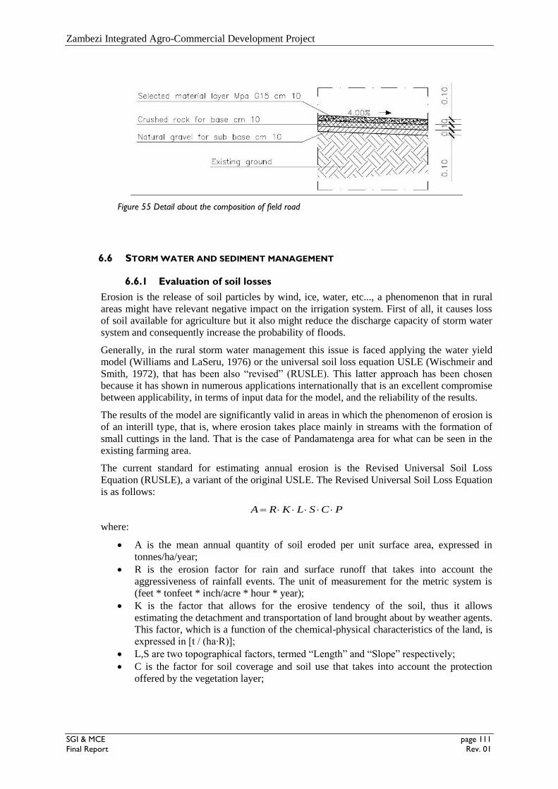
Zambezi Integrated Agro-Commercial Development Project
SGI & MCE page 111
Final Report Rev. 01
Figure 55 Detail about the composition of field road
6.6 STORM WATER AND SEDIMENT MANAGEMENT
6.6.1 Evaluation of soil losses
Erosion is the release of soil particles by wind, ice, water, etc..., a phenomenon that in rural
areas might have relevant negative impact on the irrigation system. First of all, it causes loss
of soil available for agriculture but it also might reduce the discharge capacity of storm water
system and consequently increase the probability of floods.
Generally, in the rural storm water management this issue is faced applying the water yield
model (Williams and LaSeru, 1976) or the universal soil loss equation USLE (Wischmeir and
Smith, 1972), that has been also “revised” (RUSLE). This latter approach has been chosen
because it has shown in numerous applications internationally that is an excellent compromise
between applicability, in terms of input data for the model, and the reliability of the results.
The results of the model are significantly valid in areas in which the phenomenon of erosion is
of an interill type, that is, where erosion takes place mainly in streams with the formation of
small cuttings in the land. That is the case of Pandamatenga area for what can be seen in the
existing farming area.
The current standard for estimating annual erosion is the Revised Universal Soil Loss
Equation (RUSLE), a variant of the original USLE. The Revised Universal Soil Loss Equation
is as follows:
PCSLKRA
where:
A is the mean annual quantity of soil eroded per unit surface area, expressed in
tonnes/ha/year;
R is the erosion factor for rain and surface runoff that takes into account the
aggressiveness of rainfall events. The unit of measurement for the metric system is
(feet * tonfeet * inch/acre * hour * year);
K is the factor that allows for the erosive tendency of the soil, thus it allows
estimating the detachment and transportation of land brought about by weather agents.
This factor, which is a function of the chemical-physical characteristics of the land, is
expressed in [t / (ha∙R)];
L,S are two topographical factors, termed “Length” and “Slope” respectively;
C is the factor for soil coverage and soil use that takes into account the protection
offered by the vegetation layer;

Zambezi Integrated Agro-Commercial Development Project
SGI & MCE page 112
Final Report Rev. 01
P is the conservation factor for anti-erosion practices and expresses the influence on
the soil loss of the particular arrangement of the cultivation and territorial arrangement
works carried out (not considerate in the model).
The parameter R might be calculated as:
PR 562.012.8
where P is the annual rainfall (539 mm in Pandamatenga).
The parameters L and S are estimated according to the following formula:
57415.6
43.030430
6.72
2 xxLS
m
in which:
λ is the field length in feet (2960 feet = 900 m);
m = 0.3 if field slope is less than 3% (this is on average in the study area);
x = SINƟ, where Ɵ is the slope angle (0.115° = 0.002 m/m on average).
The assigned values for parameter K, C and P are respectively 0.3, 0.08 and 0.5 on the basis of
information proposed by US EPA and included in the following tables.
Table 45 Values for parameter K to apply RUSLE method (US EPA, 1973)
Table 46 and Table 47 Values for parameter C and P to apply RUSLE method (US EPA, 1973)
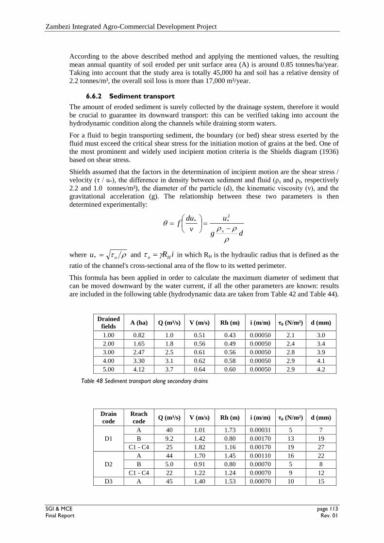
Zambezi Integrated Agro-Commercial Development Project
SGI & MCE page 113
Final Report Rev. 01
According to the above described method and applying the mentioned values, the resulting
mean annual quantity of soil eroded per unit surface area (A) is around 0.85 tonnes/ha/year.
Taking into account that the study area is totally 45,000 ha and soil has a relative density of
2.2 tonnes/m³, the overall soil loss is more than 17,000 m³/year.
6.6.2 Sediment transport
The amount of eroded sediment is surely collected by the drainage system, therefore it would
be crucial to guarantee its downward transport: this can be verified taking into account the
hydrodynamic condition along the channels while draining storm waters.
For a fluid to begin transporting sediment, the boundary (or bed) shear stress exerted by the
fluid must exceed the critical shear stress for the initiation motion of grains at the bed. One of
the most prominent and widely used incipient motion criteria is the Shields diagram (1936)
based on shear stress.
Shields assumed that the factors in the determination of incipient motion are the shear stress /
velocity (τ / u*), the difference in density between sediment and fluid (ρs and ρf, respectively
2.2 and 1.0 tonnes/m³), the diameter of the particle (d), the kinematic viscosity (ν), and the
gravitational acceleration (g). The relationship between these two parameters is then
determined experimentally:
dg
u
v
duf
s
2
**
where ou * and iRHo in which RH is the hydraulic radius that is defined as the
ratio of the channel's cross-sectional area of the flow to its wetted perimeter.
This formula has been applied in order to calculate the maximum diameter of sediment that
can be moved downward by the water current, if all the other parameters are known: results
are included in the following table (hydrodynamic data are taken from Table 42 and Table 44).
Drained
fields A (ha) Q (m³/s) V (m/s) Rh (m) i (m/m) τ0 (N/m²) d (mm)
1.00 0.82 1.0 0.51 0.43 0.00050 2.1 3.0
2.00 1.65 1.8 0.56 0.49 0.00050 2.4 3.4
3.00 2.47 2.5 0.61 0.56 0.00050 2.8 3.9
4.00 3.30 3.1 0.62 0.58 0.00050 2.9 4.1
5.00 4.12 3.7 0.64 0.60 0.00050 2.9 4.2
Table 48 Sediment transport along secondary drains
Drain
code
Reach
code Q (m³/s) V (m/s) Rh (m) i (m/m) τ0 (N/m²) d (mm)
D1
A 40 1.01 1.73 0.00031 5 7
B 9.2 1.42 0.80 0.00170 13 19
C1 - C4 25 1.82 1.16 0.00170 19 27
D2
A 44 1.70 1.45 0.00110 16 22
B 5.0 0.91 0.80 0.00070 5 8
C1 - C4 22 1.22 1.24 0.00070 9 12
D3 A 45 1.40 1.53 0.00070 10 15
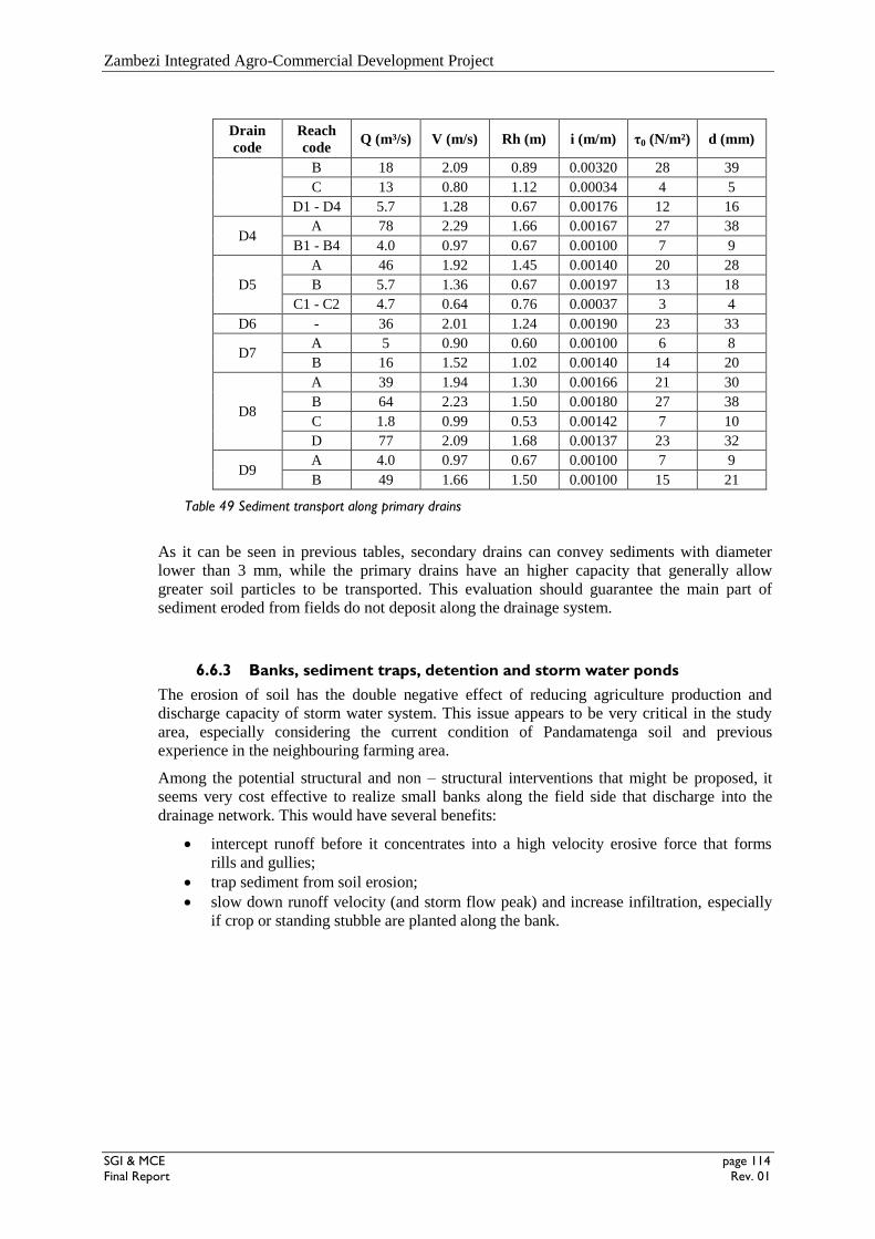
Zambezi Integrated Agro-Commercial Development Project
SGI & MCE page 114
Final Report Rev. 01
Drain
code
Reach
code Q (m³/s) V (m/s) Rh (m) i (m/m) τ0 (N/m²) d (mm)
B 18 2.09 0.89 0.00320 28 39
C 13 0.80 1.12 0.00034 4 5
D1 - D4 5.7 1.28 0.67 0.00176 12 16
D4 A 78 2.29 1.66 0.00167 27 38
B1 - B4 4.0 0.97 0.67 0.00100 7 9
D5
A 46 1.92 1.45 0.00140 20 28
B 5.7 1.36 0.67 0.00197 13 18
C1 - C2 4.7 0.64 0.76 0.00037 3 4
D6 - 36 2.01 1.24 0.00190 23 33
D7 A 5 0.90 0.60 0.00100 6 8
B 16 1.52 1.02 0.00140 14 20
D8
A 39 1.94 1.30 0.00166 21 30
B 64 2.23 1.50 0.00180 27 38
C 1.8 0.99 0.53 0.00142 7 10
D 77 2.09 1.68 0.00137 23 32
D9 A 4.0 0.97 0.67 0.00100 7 9
B 49 1.66 1.50 0.00100 15 21
Table 49 Sediment transport along primary drains
As it can be seen in previous tables, secondary drains can convey sediments with diameter
lower than 3 mm, while the primary drains have an higher capacity that generally allow
greater soil particles to be transported. This evaluation should guarantee the main part of
sediment eroded from fields do not deposit along the drainage system.
6.6.3 Banks, sediment traps, detention and storm water ponds
The erosion of soil has the double negative effect of reducing agriculture production and
discharge capacity of storm water system. This issue appears to be very critical in the study
area, especially considering the current condition of Pandamatenga soil and previous
experience in the neighbouring farming area.
Among the potential structural and non – structural interventions that might be proposed, it
seems very cost effective to realize small banks along the field side that discharge into the
drainage network. This would have several benefits:
intercept runoff before it concentrates into a high velocity erosive force that forms
rills and gullies;
trap sediment from soil erosion;
slow down runoff velocity (and storm flow peak) and increase infiltration, especially
if crop or standing stubble are planted along the bank.

Zambezi Integrated Agro-Commercial Development Project
SGI & MCE page 115
Final Report Rev. 01
Figure 56 Planimetric view and cross section of fields, drain and road to identify designed banks
This bank could be 50 cm high and it can be interrupted exclusively at the end and in the
middle of each fields (or rather every 450 m) for about 20 m.
Figure 57 Outlet scheme of storm water from fields

Zambezi Integrated Agro-Commercial Development Project
SGI & MCE page 116
Final Report Rev. 01
These openings would guarantee that the water flow collected along the banks can be totally
and continuously discharged into the secondary drains. In fact, these openings work
hydraulically like weirs thus their dimensioning makes reference to the following equation:
gHLHcQ q 2
where:
Q = flow discharged over the weir (m³/s);
cq = discharge coefficient, generally supposed equal to 0,385 when broad crested;
L = weir length (m);
H = water depth over the weir (m).
For each fields (about 900 m long) the peak discharge for the 10-years storm event is about
1.1 m³/s thus each of these openings, being every 450 m, should be allow about half of this
discharge (0.55 m³/s). According to the mentioned formula, this flow is discharged when
water depth less than 7 cm is constantly over a weir 20 m long. Runoff collect within an entire
field (1.1 m³/s) would be drained with 10 cm as water depth.
In order to prevent erosion and scour when the water flow pass beyond the openings, the drain
slope and its bottom are stabilised and protected by gabion mattresses.
Figure 58 Typical cross section of drain where field outlet is located
Figure 59 View of the drain slope where field outlet is located
When the storm water accumulates behind the banks, the irrigation fields would be then
flooded for a length that is proportional to water depth and terrain flatness. In order to avoid
such situations, the final portion of fields (a strip parallel to the bank 2.5 m wide) is properly
shaped as shown in the following picture. Therefore, before having the irrigated area flooded,

Zambezi Integrated Agro-Commercial Development Project
SGI & MCE page 117
Final Report Rev. 01
the water depth should be higher than 50 cm that means a discharge over the weir of about 12
m³/s: this peak flow for a single fields has an huge return time (100-years rainfall events is
50% higher than the 10-years, as quoted in Table 7).
Figure 60 Cross section of designed banks
Besides, along the drainage network some sediment traps can be implemented: these
structures allow for collection of sediment at single locations and reduction of downstream
maintenance requirements.
Deposition happens when the capacity of sediment transport (the shear stress that moves
sediment particles, see paragraph 6.6.2) decreases therefore the ability to effectively capture
sediment is influenced by hydrodynamic conditions (flow velocity) and type of sediment
particles (mainly size of particles). Thus the kinetic energy in the water column reduces
creating a net-depositional area. According to the already mentioned Manning’s formula (see
paragraph 6.4.2) this effect can be obtained increasing the cross section that is available for
the water flow and/or reducing the longitudinal slope.
Figure 61 Schematic functioning of sediment traps
The proposal is to create sediment trap with null longitudinal slope and bottom that is 1 m
deeper than the incoming channel; at the end of the trap the sediment would be further
hindered by a small barrage that realize a sort of weir 50 cm high over the bottom of the
channel. This type of structures should be easy to reach and to empty by machinery thus they
might be localized at the intersection between channel and roads.
Along the primary drains 26 sediments traps have been envisaged (Figure 62). They are about
25 m long and large as much as the channel where they are located. On average they can be

Zambezi Integrated Agro-Commercial Development Project
SGI & MCE page 118
Final Report Rev. 01
considered full with sediment when the deposition depth is about 1.5 m because their bottom 1
m of lower than the channel and at the end there is a barrage of about 50 cm (Figure 63).
For instance, along the drain D1 4 sediments traps are envisaged: the first one is within the
reach B where the bottom channel is 5 m wide, therefore if deposition height is 1.5 m and trap
length is 25, the sediment volume would be 5 x 1.5 x 25 = 188 m³. The subsequent reach C of
drain D1 has a bottom of 9 m thus 3 traps can accumulate 3 x 9 x 1.5 x 25 = 1,013 m³.
According to these assumptions the overall amount of sediment would be almost 9,000 m³
(see Table 50) that is about half of the annual soil erosion (see calculation in paragraph 6.6.1).
Figure 62 Positioning of sediment traps along the primary drains

Zambezi Integrated Agro-Commercial Development Project
SGI & MCE page 119
Final Report Rev. 01
Figure 63 Planimetric view and longitudinal along primary drain to identify designed sediment traps
Drain
code
Reach
code
Drain
bottom (m) Vtrap (m³) Vtot (m³)
D1
A 0 0 0
B 1 188 188
C1 - C4 3 338 1013
D2
A 0 0 0
B 1 263 263
C1 - C4 2 450 900
D3
A 1 188 188
B 1 300 300
C 0 0 0
D1 - D4 3 413 1238
D4 A 1 113 113
B1 - B4 2 338 675
D5
A 0 0 0
B 0 0 0
C1 - C2 3 263 788
D6 - 3 525 1575
D7 A 0 0 0
B 2 188 375
D8
A 1 338 338
B 1 413 413
C 0 0 0
D 1 450 450
D9 A 0 0 0
B 0 0 0
Total - - 8,817
Table 50 Estimation of sediment deposition within the sediment traps

Zambezi Integrated Agro-Commercial Development Project
SGI & MCE page 120
Final Report Rev. 01
Finally, another system has been implemented in order to collect sediments determined by soil
losses along the fields: at the end of each primary drain a detention pond has been designed.
This structure would receive water and sediment since the beginning of storm event, then its
volume would be filled up and its entrance should be closed.
Figure 64 Planimetric view of terminal portion of a primary drain and connection with detention and storm
water ponds
Their dimensioning can be roughly done considering the water volume (Vw) that would be
produced during the first half an hour of the storm event. With reference to peak discharges
(for about 12 hours) included in Table 43, the side length of square detention ponds is
calculated considering about 2 m as height. The resulting overall volume would be more than
7,000 m³.
Drain
code Q (m³/s) Vw (m³) Lpond (m)
D1 1.7 752 19
D3 1.9 834 20
D4 3.3 1,469 27
D5 1.9 853 21
D6 1.5 671 18
D7 0.7 302 12
D8 3.2 1,443 27
D9 2.0 914 21
Total - 7,238 -
Table 51 Dimensioning or detention ponds

Zambezi Integrated Agro-Commercial Development Project
SGI & MCE page 121
Final Report Rev. 01
In this way the sediment, but also water with higher content of fertilizers, would be
accumulated for deposition: at a later time sediments could be collected, analyzed, treated (if
needed) and reuse.
This would minimized also the discharge of fertilizers in the natural environment. However, in
order to control water drained from fields and replace natural ponds within the study area,
some storm water ponds have been envisaged downstream the detention ponds.
The suggested volume of this structure could be about 20,000 m³ thus, being at the end of the
8 primary drains, their overall volume would be 160,000 m³. This water amount is far from the
storm water volume estimated in paragraph 6.3.4 (124 Mm³) because its accumulation would
be high costly and probably not necessary. They would reasonable be filled for each rainy
event occurring in the study area and generating some runoff.
These structures are mainly a proposal to compensate the natural water ponds that are
currently within the study area and would be substitute by the irrigation fields. Rough
estimation on the basis on satellite imagery and topographic survey has lead to delimitate an
overall extension for existing water pans of about 0.9 km². If it is assumed they have about 30
cm of water depth on average, their total volume is 270,000 Mm³, thus the proposed storm
water ponds would recover the 60% of them.
6.7 DRAIN MAINTENANCE
A long-term drainage maintenance plan shall be implemented to ensure that the storm water
management system functions as designed. This is mainly to avoid, or at least to minimize,
reduction in discharge capacity of channels and, consequently, increase the risk of floods and
damages to agricultural practise.
This plan is intended to cover all drainage structures that are represented by primary and
secondary drains, but also by sediment traps, detention ponds and storm water ponds. These
latter infrastructures, as already explained in paragraph 6.6, have been envisaged exactly to
facilitate the maintenance of the drainage system.
The storm water management system protects and enhances the storm water runoff water
quality through the removal of sediment and pollutants, and source control significantly
reduces the amount of pollutants entering the system. This is particularly important because
within the drained area there will be use of fertilized and because the natural environment is
particularly sensitive.
The MoA possesses the primary responsibility for overseeing and implementing the
maintenance plan and designating a person who will be responsible. This responsible and
maintenance staff will conduct the maintenance program and they will ensure that inspections
and record keeping are timely and accurate and that cleaning and maintenance are performed
at least on a bi-annual basis.
A Log Forms is typically compile including the date and the amount of the last significant
storm event in excess of a certain rainfall depth in a 24-hour period (10 mm could be the
threshold), physical conditions of channel bottom and slope (erosion), depth of sediment,
evidence of overtopping of the field banks or debris blockage at the culverts.
Records of maintenance will be kept on file at the responsable’s office and copies of
maintenance log sheets indicating all work and inspections will be available upon request. All
storm water management structures will be inspected two times per year, before the beginning
of rainy season (November) and a month after the first heavy rain (January), as site conditions
warrant.

Zambezi Integrated Agro-Commercial Development Project
SGI & MCE page 122
Final Report Rev. 01
7 COST ESTIMATION AND WORK PLAN
For the drafting of the bill of quantity, unit prices used for previous projects done in other
African countries have been used as reference and, in some cases, surveys have been carried
out.
The prices are in Pula, local currency in Botswana. The exchange rate to Euro (at the moment
of the document drafting) is: 1 euro = 11.569 Pula. The total amount for the works is
2,298,581,477.14 Pula (equivalent to 198,684,542.93 euro).
The document is divided in chapters that correspond to complete works and chapters contains
specific articles about each work. Here below the description of the chapters.
General Provision
This chapter is related to the general and temporary works paid to the Company. Particularly
the temporary fence of the area (accommodation, offices, laboratories available for the
Construction Supervision) and the temporary signposting of the construction site.
Land grading
The chapter pertains to the first operation of cleaning the area from vegetation and the second
operation of set up of the superficial layout of the ground.
Main Drains
This chapter pertains to the operation of leveling the ground according to the elevations
defined in the project with the related earthworks and backfill.
Then the main channels will be carried out with the geometric characteristics planned in the
specific relations. The section of the channel will be trapezoidal with bank slope of 2/1. Part of
the earthworks will need the use of the hydraulic hammer due the presence of rocks.
Secondary Drains
This chapter pertains to the operation of leveling the ground according to the elevations
defined in the project with the related earthworks
Then the main channels will be implemented with the geometric characteristics planned in the
specific relations. The section of the channel will be trapezoidal with bank slope of 2/1. Part of
the earthworks will need the use of the hydraulic hammer do the presence of rocks.
Drain Crossing
In case drains cross the roads, cast-in-place reinforced concrete culverts will be used. For
concrete Class C40 will be used as well as reinforced steel bars.
Sediment Trip
Lower areas will be placed along the channels to block sediments. Part of the earthworks will
need the use of the hydraulic hammer. A concrete weir will be placed.

Zambezi Integrated Agro-Commercial Development Project
SGI & MCE page 123
Final Report Rev. 01
Primary irrigation pipe
For the primary irrigation network, cast in place concrete slab will be done and FRB
FIBERGLASS PIPE with different diameter will be used, surrounding them with sand and
arid material. Network development is 89 km.
Secondary irrigation pipe
Also in this case FRB FIBERGLASS PIPE will be used. Network development is 325 km.
Detention pond
The detentions pond will be carried out with earthwork and rock excavation. An adequate
metal gate will be put in place with connected structures in reinforced concrete.
Stormwater pond
The detentions pond will be implemented with earthwork and rock excavation. An adequate
metal gate will be put in place with connected structures in reinforced concrete.
Primary e secondary roads
Primary roads will have carriageway of 6 m (3 m for each lane) with two shoulders of 1.5 m.
Total 9 m
Tertiary roads will have carriageway of 5 m (2.5 m for each lane) with two shoulders of 1 m.
Total 7 m
The road package will be done with starting from the lower layers
- Natural gravel for sub base cm 20
- Crushed rock for base cm 20
- Selected material layer G15 Mpa cm 15
- Total cm 55
On the basis of designed longitudinal profile, excavation and backfill will be defined. In case
of excavation it has been envisaged a certain percentage in rock, while for backfill excavation
material will be used after being compressed according to a layer of about 50 cm.
Along the road small retaining walls will be probably carried out. An exiguous quantity of
gabions and pavements have been considered. Adequate signals will be positioned. It has to be
underlined that a top layer with material G15 Mpa will be finally realized. It is also envisaged
lateral channel to collect water drained along the road.

Zambezi Integrated Agro-Commercial Development Project
SGI & MCE page 124
Final Report Rev. 01
Field roads
Tertiary roads will have a carriageway of 4 m (2 m for each lane):
The road package will be done with starting from the lower layers
o Natural gravel for sub base cm 10
o Crushed rock for base cm 10
o Selected material layer G15 Mpa cm 10
o Total cm 30
Main Pumping station
The pumping station will be realized with reinforced concrete with pups that will lift the
design discharge. 9 pumps (7 main pumps + 2 secondary pumps), Q = 3 m3/s and H = 50 m
have been envisaged. Total of 12.5 MW.
The work will be completed with mechanical components, pipes, valves, wiring, switchboard
and civil works. A transform plant will be built upstream the pumping station.
Electrified fence
An electrified fence 3 m high of galvanized metal that leans to reinforced concrete plinth will
be realized. It will be equipped with low voltage cables (24 Volt) each meter along the height
to avoid intrusions.
Transportation
4 million cubic meter of earth are foreseen will be displaced and used on the site or moved to
another placed suggested by the Administration within the next 20 km. The first meter of
earthwork will be reused for the new embankment.
Center pivot sprinkler
The cost for center pivot irrigation system contains mainly the total cost of the unit. There are
275 center pivot units designed for the net irrigation command area of 15,000 ha. Moreover,
the cost for 275 three phase generators are also include
Drip irrigation system
The cost for drip irrigation contains for the lateral and manifold pipes with diameter of 25 mm
and 110 mm respectively for 10,000 ha. Beside this, the cost for auxiliary components like
measurement devices, water control valves, fertilizer applicators and all other fittings
Typical Farmstead infrastructure
This infrastructure is composed by:
• Project housing & services;
• Satellite village
• Office facilities

Zambezi Integrated Agro-Commercial Development Project
SGI & MCE page 125
Final Report Rev. 01
• Mechanical facilities, workshop
• Storage facilities
Here below a brief description of the mentioned infrastructures is given, while graphical
representation of them can be found in the drawings attached to the present report.
Project Housing and Services
The typical housing and services designed at this stage of the feasibility study of this project is
a service quarter, which contains living quarter (bedroom), dining room, kitchen, shower,
toilet.
Satellite village
The general planning criteria adopted for the village’s establishment are as follows:
• Villages should be located to minimize travel distances to work area;
• Villages should be located on non-irrigable land, as much as possible, and where possible in
a well drained land;
• Villages should be located away from irrigation infrastructures and open drains where
possible to be free from the effects of water born diseases.
Hence, the typical design of these villages contains living quarter (bedroom), dining room,
kitchen, shower, toilet.
Office facilities
The typical office complex designed at this stage of the feasibility study of this project
contains office, conference room, archives, store, toilet, casher room.
Mechanical facilities (workshop)
The typical farm workshop was designed for mechanical maintenance of farm machineries
and others. This workshop contains office, welding bay, inspection pits, oil and lubricant
store, sinks, toilet, hand washbasin.
Storage facilities
Typical design of on-farm storage facility was done for this project as one of the farmsteads.
The storehouse is mainly for the purpose of storing farm input and produces. It contains office
for the staff and the storehouses.

Zambezi Integrated Agro-Commercial Development Project
SGI & MCE page 126
Final Report Rev. 01
A first hypothesis of project work plan showing the work breakdown phasing is reported in
the following table.

Zambezi Integrated Agro-Commercial Development Project
SGI & MCE page 127
Final Report Rev. 01
8 FINAL CONSIDERATION ABOUT ZIACDP FEASIBILITY
As per the ToR, pressurized irrigation system has been considered for the project area. For this
depending on the soil type, both sprinkler and drip irrigation systems have been selected.
Due to several reasons listed in the document, continuous sprinkler irrigation system was
taken for design as compared to the conventional sprinkler system. Out of several continuous
sprinkler systems, for the same reason, centre pivot sprinkler has been selected and designed
on sandy clay loam, sand loam and loamy sand soils at 17,814 ha net and 15,000 cropped area.
For sandy soils of the project area, drip irrigation system has been designed at 10,554 net area
and 10,000 ha cropped area. Moreover, 15,000 ha has been allotted for both three wet
(Sorghum, Sunflower and Beans) and four dry season crops (Maize, Wheat, Soybean and
Alfalfa).
From this, the monthly water demand for both wet and dry season as supplementary and full-
fledge irrigation supply ranges from 10.43 Mm³ to 42.08 Mm³ during December and
September respectively.
In general, the investigation of the current feasibility study shows that the project area can be
used for pressurized irrigation development, bearing in mind that application of some of the
correction measures recommended are implemented in order to improve the production of
crops and sustainability of soil fertility.
Therefore, it could be concluded that pressurized irrigation system is technically feasible for
Zambezi Integrated Agro-Commercial Development Project.

Zambezi Integrated Agro-Commercial Development Project
SGI & MCE page 128
Final Report Rev. 01
9 ANNEXES
9.1 SOIL PHYSICAL AND CHEMICAL PROPERTIES
Within the following tables:
Infiltration is the Basic Infiltration Rate;
HC is Hydraulic conductivity;
AWC is Available Water holding Capacity.
9.1.1 Soil parameters from profile pits on sandy soils
Code East North pH (0-30) Infiltration
(cm/hr) HC(m/day)
AWC (mm/m)
P2 344150 7928820 5.3
P3 341540 7928290 5.7
p4 340140 7928380 5.7
p6 342523 7929808 6.6 45.4 34.4
P7 348384 7929442 6.2
P8 350980 7929718 5.9 22.9 23.3
P10 347362 7927467 5.0 60.4
P11 342950 7927734 5.2 33.2 10.5
P12 337415 7931960 6.5
P13 339744 7929600 5.7
P14 336975 7929870 4.9
P15 336758 7927885 6.0 60.6
P16 335609 7928377 5.5 27.9 23
P18 330000 7932435 6.2 20.2 21.9 69.2
P20 325891 7929286 5.8 19.9 13.2
P21 328402 7928377 5.3 34.7 13.2
P22 335609 7931558 5.9 30.6 12.2
P23 334630 7930000 4.7 16.7 24.1 68.5
P25 330935 7930115 5.6
P26 330341 7928232 6.1
P30 337412 7932737 5.5
P32 336749 7933991 6.8
P33 337135 7937400 6.0
P34 335947 7937307 5.0
P35 334715 7936804 5.1
P36 332505 7937300 6.0
P37 331238 7937250 6.8
P39 326189 7937300 6.2
P41 320663 7937550 5.8 22.7 31 60.8
P44 325807 7935560 5.5
P45 328950 7936138 7.2 19.1 9.1

Zambezi Integrated Agro-Commercial Development Project
SGI & MCE page 129
Final Report Rev. 01
Code East North pH (0-30) Infiltration
(cm/hr) HC(m/day)
AWC (mm/m)
P48 330325 7935000 5.7
P50 319908 7932450 5.3 14.2 6.8
P51 327000 7932450 6.1 11.6 6.8
P52 332600 7935975 6.1 19.1 16.2
P54 327918 7940245 5.6 19.1 6.1
P57 322834 7941726 5.5
P58 322571 7939555 5.5
P59 325463 7939199 6.5 56.0
P60 332777 7938719 5.0 32.7 11.5
P62 328385 7942750 4.69 65.7
P67 330938 7940853 6.2
P68 334633 7940220 5.4
P69 332020 7942400 6.5
P70 335344 7938364 6.2
P71 337960 7947950 5.58 32.8 23.6
P73 334554 7947276 5.71
P77 331138 7947500 5.1
P78 334138 7942900 5.5
P80 324000 7945000 5.5
P81 327000 79475000 32.5 10.7
P82 333238 7944049 5.07
P83 336650 7943963 22.5 21
P84 337707 7946197 5.9
P85 338113 7948313 5.0
P86 339000 7949613 5.4
P87 336650 7949288 6.5
P89 333000 7948313 5.1
P90 329900 7948800 5.9
P91 328138 7948475 5.8 57.7
P92 325788 7948475 5.9 29.8 37.9
P93 330000 7950000 6.4
P94 338804 7939225 6.4 26.8 25.1
P95 341324 7940304 5.3 58.4
P99 345440 7937628 4.9
P100 342898 7937763 5.3 50.2 38.9
P101 341212 7938482 5.1
P102 339771 7936795 5.3
Average 5.71 26.57 19.11 61.92

Zambezi Integrated Agro-Commercial Development Project
SGI & MCE page 130
Final Report Rev. 01
9.1.2 Soil parameters from profile pits on loamy sand soils
Code East North pH (0-30) Infiltration
(cm/hr) HC(m/day)
AWC (mm/m)
P1 352335 7927848 5.0 0.8 2.3
P17 334225 7932160 5.5 1.4 0.7 60.3
P38 330474 7936847 7.7
P40 324963 7937209 6.0
P46 333000 7933963 6.1
P49 323997 7934071 6.3 19.9 18.9 87.5
P53 331950 7934288 5.8 11.7 8.8
P55 326165 7941910
8.5 8.8
P56 324277 7942783
13.7 9.8
P61 329295 7937650 5.9 2.5 1.2 59.8
P74 335400 7945803 5.96 15.4 1.3 98.2
P88 334950 7948475 5.4 6.8 1.6 68.0
P96 342696 7939652 5.0
P97 345755 7939405 5.5
87.2
P98 346767 7938437 5.1 28.3 10.3
Average 5.78 10.9 6.37 76.85
9.1.3 Soil parameters from profile pits on sandy loam soils
Code East North pH (0-30) Infiltration
(cm/hr) HC(m/day)
AWC (mm/m)
P5 338440 7928235 7.4 2.4 2.4
P9 338225 7931438 7.6 6 2.4 78.5
P19 325304 7931558 7.1 4.6 1.7
P24 328250 7930400 6.0
P27 333029 7927590 6.4
P28 332490 7932403 7.8
P31 336250 7932800 6.1 4.2 2.3 81.4
P42 335076 7933700 7.6 5.8 4.2 92.5
P43 335180 7934816
4.8 3.4
P75 328131 7945051 6.43
P79 327661 7943422 6.1 5.3 1.4 88.1
Average 6.93 4.73 2.54 85.11

Zambezi Integrated Agro-Commercial Development Project
SGI & MCE page 131
Final Report Rev. 01
9.1.4 Soil parameters from profile pits on sandy loam soils
Code East North pH (0-30) Infiltration
(cm/hr) HC(m/day)
AWC (mm/m)
P47 328985 7933649 6.8 6.1 3.7
P63 334633 7941348
3.3 1.7
P64 337218 7938859
2.4 3.1
P65 336313 7942780 6.5 3.7 2.3
P72 336513 7947900 5.75 1 1.8
P76 331625 7945000 6.0 0.6 3.3 97.2
Average 6.3 2.9 2.7 97.2

Zambezi Integrated Agro-Commercial Development Project
SGI & MCE page 132
Final Design Report Rev. 01
9.2 CALCULATION RELATED TO CROP WATER REQUIREMENT
9.2.1 Details of crop water requirement for sorghum as a supplementary irrigation
Crop-SORGHUM Area 6,750 P Date Nov. 15
Jan Feb Mar Apr May Jun Jul Aug Sep Oct Nov Dec
Crop Factor(Kc) 0.91 0.93 0.56 0.15 0.64
ETo (mm) 144.46 134.68 139.5 157.5 149.11
ETc (mm) 131.88 125.84 78.75 23.63 94.76
Mean Monthly Rainfall (mm) 136.00 112 65 21 1 0.8 0 0 1.5 23 65 114
Effective Rainfall (ER) (mm) 83.80 64.60 29.00 2.60 0.00 0.00 0.00 0.00 0.00 3.80 29.00 66.20
Net Irrigation Requirement
(mm) 48.08 61.24 49.75 0.00 0.00 28.56
Field Irrigation Requirement
(mm) 60.10 76.54 62.19 0.00 77.00 0.00 35.70
Field Irrigation Requirement
(mm/day) 1.94 2.73 2.49 0.00 1.15
Crop Water Needs(l/s/ha) 0.22 0.32 0.29 0.00 0.13
Flow (l/s) 1517.9 2140.5 1947.71 0.00 901.62
Mm^3 4.07 5.18 4.21 0.00 2.41

Zambezi Integrated Agro-Commercial Development Project
SGI & MCE page 133
Final Design Report Rev. 01
9.2.2 Details of crop water requirement for sunflower as a supplementary irrigation
Crop-SUNFLOWER Area 3,750 P Date Dec. 1
Jan Feb Mar Apr May Jun Jul Aug Sep Oct Nov Dec
Crop Factor(Kc) 0.76 1.05 0.86 0.19 0.38
ETo (mm) 144.46 134.68 139.5 126 149.11
ETc (mm) 109.28 141.41 119.7 23.52 56.28
Mean Monthly Rainfall (mm) 136.00 112 65 21 1 0.8 0 0 1.5 23 65 114
Effective Rainfall (ER) (mm) 83.80 64.60 29.00 2.60 o 0.00 0.00 0.00 0.00 3.80 29.00 66.20
Net Irrigation Requirement
(mm) 25.48 76.81 90.70 0.00 0.00
Field Irrigation Requirement
(mm) 31.85 96.02 113.38 0.00 0.00
Field Irrigation Requirement
(mm/day) 1.03 3.43 4.05 0.00 0.00
Crop Water Needs(l/s/ha) 0.12 0.40 0.47 0.00 0.00
Flow (l/s) 446.87 1491.70 1761.36 0.00
Mm^3 1.20 3.61 4.72 0.00 0.00
9.2.3 Details of crop water requirement for beans as a supplementary irrigation
Crop-BEANS Area 3,000 P Date Dec. 15
Jan Feb Mar Apr May Jun Jul Aug Sep Oct Nov Dec
Crop Factor(Kc) 0.65 1.01 0.84 0.09 0.15
ETo (mm) 144.46 134.68 139.5 126 149.11
ETc (mm) 93.67 136.3635 117.675 10.92 23.088
Mean Monthly Rainfall (mm) 136.00 112 65 21 1 0.8 0 0 1.5 23 65 114
Effective Rainfall (ER) (mm) 83.80 64.60 29.00 2.60 0.00 0.00 0.00 0.00 0.00 3.80 29.00 66.20
Net Irrigation Requirement
(mm) 9.87 71.76 88.68 0.00 0.00
Field Irrigation Requirement
(mm) 12.33 89.70 110.84 0.00 0.00
Field Irrigation Requirement
(mm/day) 0.40 3.20 3.58 0.00
Crop Water Needs(l/s/ha) 0.05 0.37 0.41 0.00
Flow (l/s) 138.44 1114.90 1244.31
Mm^3 0.37 2.70 3.33 0.00
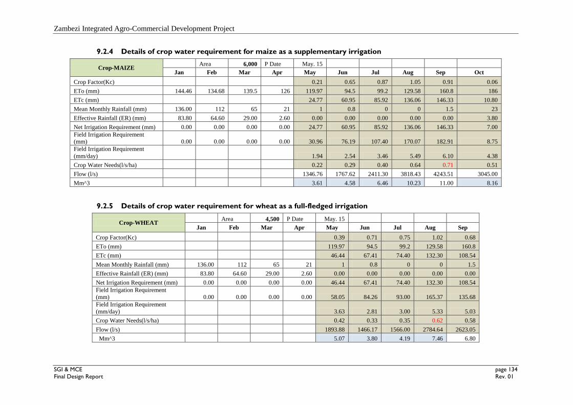
Zambezi Integrated Agro-Commercial Development Project
SGI & MCE page 134
Final Design Report Rev. 01
9.2.4 Details of crop water requirement for maize as a supplementary irrigation
Crop-MAIZE Area 6,000 P Date May. 15
Jan Feb Mar Apr May Jun Jul Aug Sep Oct
Crop Factor(Kc) 0.21 0.65 0.87 1.05 0.91 0.06
ETo (mm) 144.46 134.68 139.5 126 119.97 94.5 99.2 129.58 160.8 186
ETc (mm) 24.77 60.95 85.92 136.06 146.33 10.80
Mean Monthly Rainfall (mm) 136.00 112 65 21 1 0.8 0 0 1.5 23
Effective Rainfall (ER) (mm) 83.80 64.60 29.00 2.60 0.00 0.00 0.00 0.00 0.00 3.80
Net Irrigation Requirement (mm) 0.00 0.00 0.00 0.00 24.77 60.95 85.92 136.06 146.33 7.00
Field Irrigation Requirement
(mm) 0.00 0.00 0.00 0.00 30.96 76.19 107.40 170.07 182.91 8.75
Field Irrigation Requirement
(mm/day) 1.94 2.54 3.46 5.49 6.10 4.38
Crop Water Needs(l/s/ha) 0.22 0.29 0.40 0.64 0.71 0.51
Flow (l/s) 1346.76 1767.62 2411.30 3818.43 4243.51 3045.00
Mm^3 3.61 4.58 6.46 10.23 11.00 8.16
9.2.5 Details of crop water requirement for wheat as a full-fledged irrigation
Crop-WHEAT Area 4,500 P Date May. 15
Jan Feb Mar Apr May Jun Jul Aug Sep
Crop Factor(Kc) 0.39 0.71 0.75 1.02 0.68
ETo (mm) 119.97 94.5 99.2 129.58 160.8
ETc (mm) 46.44 67.41 74.40 132.30 108.54
Mean Monthly Rainfall (mm) 136.00 112 65 21 1 0.8 0 0 1.5
Effective Rainfall (ER) (mm) 83.80 64.60 29.00 2.60 0.00 0.00 0.00 0.00 0.00
Net Irrigation Requirement (mm) 0.00 0.00 0.00 0.00 46.44 67.41 74.40 132.30 108.54
Field Irrigation Requirement
(mm) 0.00 0.00 0.00 0.00 58.05 84.26 93.00 165.37 135.68
Field Irrigation Requirement
(mm/day) 3.63 2.81 3.00 5.33 5.03
Crop Water Needs(l/s/ha) 0.42 0.33 0.35 0.62 0.58
Flow (l/s) 1893.88 1466.17 1566.00 2784.64 2623.05
Mm^3 5.07 3.80 4.19 7.46 6.80

Zambezi Integrated Agro-Commercial Development Project
SGI & MCE page 135
Final Design Report Rev. 01
9.2.6 Details of crop water requirement for soybean as a full-fledged irrigation
Crop-SOYBEAN Area 3,000 P Date Jun. 15
Jan Feb Mar Apr May Jun Jul Aug Sep Oct
Crop Factor(Kc) 0.18 0.69 1.01 1.05 0.71
ETo (mm) 47.25 99.2 129.58 160.8 168
ETc (mm) 8.27 68.00 131.04 168.84 118.68
Mean Monthly Rainfall (mm) 136.00 112 65 21 1 0.8 0 0 1.5 23
Effective Rainfall (ER) (mm) 83.80 64.60 29.00 2.60 0.00 0.00 0.00 0.00 0.00 3.80
Net Irrigation Requirement (mm) 0.00 0.00 0.00 0.00 0.00 8.27 68.00 131.04 168.84 114.88
Field Irrigation Requirement
(mm) 0.00 0.00 0.00 0.00 0.00 10.34 85.00 163.80 211.05 143.60
Field Irrigation Requirement
(mm/day) 0.69 2.74 5.28 7.04 5.13
Crop Water Needs(l/s/ha) 0.08 0.32 0.61 0.82 0.59
Flow (l/s) 239.79 954.19 1838.83 2448.18 1784.80
Mm^3 0.62 2.56 4.93 6.35 4.78
9.2.7 Details of crop water requirement for alfalfa as a full-fledged annual irrigation
Crop-ALFALFA Area 1,500 P Date Jan. 1
Jan Feb Mar Apr May Jun Jul Aug Sep Oct Nov Dec
Crop Factor(Kc) 0.9 0.9 0.9 0.9 0.9 0.9 0.9 0.9 0.9 0.9 0.9 0.9
ETo (mm) 144.46 134.68 139.5 126 119.97 94.5 99.2 129.58 160.8 186 157.5 149.11
ETc (mm) 130.01 121.21 125.55 113.40 107.97 85.05 89.28 116.62 144.72 167.40 141.75 134.20
Mean Monthly Rainfall (mm) 136.00 112 65 21 1 0.8 0 0 1.5 23 65 114
Effective Rainfall (ER) (mm) 83.80 64.60 29.00 2.60 0.00 0.00 0.00 0.00 0.00 3.80 29.00 66.20
Net Irrigation Requirement (mm) 46.21 56.61 96.55 110.80 107.97 85.05 89.28 116.62 144.72 163.60 112.75 68.00
Field Irrigation Requirement (mm) 57.77 70.77 120.69 138.50 134.97 106.31 111.60 145.78 180.90 204.50 140.94 85.00
Field Irrigation Requirement
(mm/day) 1.86 2.53 3.89 4.62 4.35 3.54 3.60 4.70 6.03 6.60 4.70 2.74
Crop Water Needs(l/s/ha) 0.22 0.29 0.45 0.54 0.51 0.41 0.42 0.55 0.70 0.77 0.54 0.32
Flow (l/s) 324.24 439.75 677.41 803.30 757.55 616.61 626.40 818.24 1049.22 1147.84 817.44 477.09
Mm^3 0.87 1.06 1.81 2.08 2.03 1.60 1.68 2.19 2.72 3.07 2.12 1.28
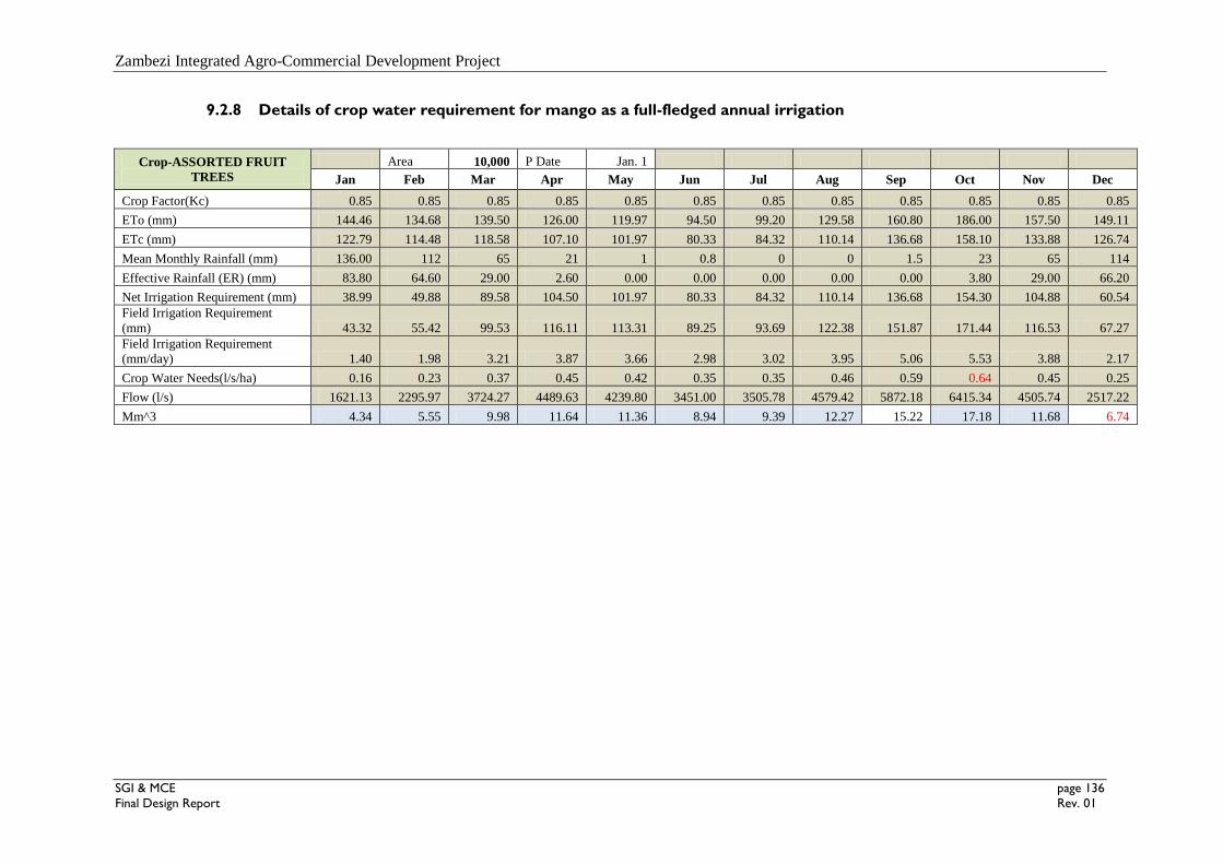
Zambezi Integrated Agro-Commercial Development Project
SGI & MCE page 136
Final Design Report Rev. 01
9.2.8 Details of crop water requirement for mango as a full-fledged annual irrigation
Crop-ASSORTED FRUIT
TREES
Area 10,000 P Date Jan. 1
Jan Feb Mar Apr May Jun Jul Aug Sep Oct Nov Dec
Crop Factor(Kc) 0.85 0.85 0.85 0.85 0.85 0.85 0.85 0.85 0.85 0.85 0.85 0.85
ETo (mm) 144.46 134.68 139.50 126.00 119.97 94.50 99.20 129.58 160.80 186.00 157.50 149.11
ETc (mm) 122.79 114.48 118.58 107.10 101.97 80.33 84.32 110.14 136.68 158.10 133.88 126.74
Mean Monthly Rainfall (mm) 136.00 112 65 21 1 0.8 0 0 1.5 23 65 114
Effective Rainfall (ER) (mm) 83.80 64.60 29.00 2.60 0.00 0.00 0.00 0.00 0.00 3.80 29.00 66.20
Net Irrigation Requirement (mm) 38.99 49.88 89.58 104.50 101.97 80.33 84.32 110.14 136.68 154.30 104.88 60.54
Field Irrigation Requirement
(mm) 43.32 55.42 99.53 116.11 113.31 89.25 93.69 122.38 151.87 171.44 116.53 67.27
Field Irrigation Requirement
(mm/day) 1.40 1.98 3.21 3.87 3.66 2.98 3.02 3.95 5.06 5.53 3.88 2.17
Crop Water Needs(l/s/ha) 0.16 0.23 0.37 0.45 0.42 0.35 0.35 0.46 0.59 0.64 0.45 0.25
Flow (l/s) 1621.13 2295.97 3724.27 4489.63 4239.80 3451.00 3505.78 4579.42 5872.18 6415.34 4505.74 2517.22
Mm^3 4.34 5.55 9.98 11.64 11.36 8.94 9.39 12.27 15.22 17.18 11.68 6.74

Zambezi Integrated Agro-Commercial Development Project
SGI & MCE page 137
Conceptual Design Report Rev. 01
9.3 FLOW CHART OF CONTINUOUS MOVE SPRINKLER SYSTEM DESIGN
Basic Farm Data
`
i) Preliminary design Factors
ii) Final Design Steps
Soils Crops
Map of design Area Water Quantity and Quality
Water intake rate
Irrigation Interval
Amount per Application
Peak water use Root zone depth Depletion Water Holding Capacity
Application rate
Determination of pipe Sizes
Minimum Allowable Flow Rate
Sprinkler
Selection
System Capacity
Flow Chart: Design of Continuous-Move sprinkler system
Selection of other components- Fittings
Draw Map of Design
Make list of Materials
Operation instructions
Total Dynamic Head
Selection of pump and power
Units
Towpath spacing Irrigation Interval Re-adjusted Travel Speed

Zambezi Integrated Agro-Commercial Development Project
SGI & MCE page 138
Final Design Report Rev. 01
9.4 DESIGN TABLE OF DRIP IRRIGATION SYSTEM
DU Type L50/E2
This will work on max. manifold Elevation difference + or - 1.5 m
Pipe Size Determination
2
1. Lateral
Flow
rate,Ql(m3/h
)
External
dia,
Do(mm)
Internal
dia,Di(m
m)
Hydraul
ic
gradient,
J (0/00)
Length,l
(m) F
Head
loss,hf(m
)
Average
Horizontal
slope (crop
direction) in
all BDU's, z
(%)
Average
operating H
of dripper -
nominal
s(
m)
Hi (lateral
inlet H),(m)
Hd(H at
the closed
end of the
lateral),(m
)
i -
Hd
(differenc
e b/n first
and last
dripper),(
m)
0.37 25 20.8 0.81 292 .37 0.87 0.05 15 0.15 15.73 14.71 1.02
Check for 20% rule, ∆h= 1.02 Ok!
Check for 50% of 20% , ∆h= 1.02 Ok!
For practical limits shall be less than 50% of allowable pressure
difference
2. Manifold
Flow
rate,Qm(m3/
h)
External
dia,Do(m
m)
Internal
dia,Di(m
m)
Hydraul
ic
gradient
(0/00)
Length ,
l
(m)
F
Head
loss,hf(m
)
Average
vertical slope
in all BDU’s,
z (%)
Hi (lateral
inlet H),(m)
Hm
(manifold
inlet H)
Hd(H of
last
dripper),(
m)
m -
Hd
(differenc
e b/n
manifold
inlet and
last
dripper),(
m)
16.685 110 105.6 0.28 447.00 0.37 0.46 0.20 15.73 0.89 16.52 14.71 1.81

Zambezi Integrated Agro-Commercial Development Project
SGI & MCE page 139
Final Design Report Rev. 01
3. Down ward riser pipe(connect to manifold)
Flow rate,
Q
(m3/h)
External
dia, Do
(mm)
Internal
dia, Di
(mm)
Hydraulic
gradient
(0/00)
Length
(m) F
Head
loss, hf
(m)
Average
Horizontal
slope along
the connecter
pipe, z (%)
Hm (manifold
inlet H)
Hc
(connector
pipe inlet
H)
Hd (H of last
dripper),
(m)
c -Hd
(difference
b/n
connector
pipe inlet
and last
dripper),
(m)
16.685 110 105.6 0.28 1.50
1
.
0
0 0.00 0 16.52
0
0 16.02 14.71 1.32
4. Upward riser
4.1 Head loss
Flow rate,
Q (m3/h)
External
dia, Do
(mm)
Internal
dia,
Di(mm)
Hydraulic
gradient,
J (0/00)
Length, l
(m) F
Head
loss, h
f(m)
Average
vertical
slope, z (%)
Hc (connector
pipe inlet H)
Hr(riser
pipe
inlet H)
33.37 110 105.6 0.95 1.80
1
.
0
0 0.02 0 16.02 1.80 16.94

Zambezi Integrated Agro-Commercial Development Project
SGI & MCE page 140 Final Design Report Rev. 01
4.2. Operating head pressure
* Loss in the field head control-valve (m) 5
** Riser pipe Hr(m) 16.94
Summed to 21.94