LA-6943-HHistory

C3●

I

.

(NC-14 REPORT COLLECTION UC-32

REPR(XXKYrKW Issued: May 1978

CX)PY

Computing at LASL in the 1940s and 1950s

Roger B. LazarusEdward A. Voorhees

Mark B. WellsW. Jack Worlton

h:10s alamosscientific laboratory

of the University of CaliforniaLOS ALAMOS, NEW MEXICO 87545

An Affirmative Action/Equal Opportunity Employer

UNITED STATES

DEPARTMENT OF ENERGY

CONTRACT W-7405 -ENG. 36

. - “. --*

Prin!cd in the United St.Ites of Amcrkm. AviMJIc fmrnNational Tc.hnical Inbrnatlu” SmvICe

US. 13cpartment of CummcrccS285 Pu,! Royal R(,.dSprin$licld. VA 22161

Micru81idw s 3.OO

0014325 4.00 126.150 7,25 15 I-275 10.75 376400 13,00 501-525 15.25026.0S0 4.50 1s!.17s 8.00 276.3 (IO 1I ,00 401-42S 13.25 S26.5S0 15.SO051.075 $.25 176.200 9.00 3(21.325 11,7S 426450 14,00076-100 6.00

SS1+7S 16.M20!.225 9,25 326.3S0 12.00 45147s 14.s0

101-12s 6.3oS76400 16.50

226.2S0 9.5n 3s1.375 I 2s0 476.500 15.00 601.IJP --1

1. Add S2.S0 for each additmnal 10 I2.Pw mcremenl from WI pages up.

Thm report was pmparrd u an account O( work spo”somdby the U“tled States Gc.vmnnm”t. Netther the Umted SUtesnot the United Slates Department 01 Energy. nor anv of theiremployees. nor any of thetr contract.”. subcc.nltactc.m. ortheir employees. makes anY warranty, ●xDces$ or implied. orassumes any Ieml Iiabibty or responsibility lot the .ccuracy.COlnplete”ess. 0. usefulness 01 any I“fom. ti. n. app.,.tus.pr.duct. or Pcocess disclosed. or rrprewnts that iu use wouldnot infringe Privately owned rlchls.

PREFACE

Each year the National Computer Conference devotes a session, known asPioneer Day, to recognizing a pioneer contributor to the computing profession.

The 1977 National Computer Conference was held in Dallas, Texas on June 13-16, 1977, and the hosts of the conference honored the Los Alamos ScientificLaboratory at the associated Pioneer Day. Since digital computation at LASLhas always been a multifaceted and rapidly changing activity, the record of itshistory is somewhat fragmentary. Thus the 1977 Pioneer Day gave us the oppor-tunity to survey and record the first 20 years of digital computation at LASL.Four talks were presented:

I. “Hardware” by W. Jack Worlton,

II. “Software and Operations” by Edward A. Voorhees,IH. “MANIAC” by Mark B. Wells, andIV. “Contributions to Mathematics” by Roger B. Lazarus.

The contents of this report were developed from those talks. Each of them sur-veys its subject for the 1940s and 1950s. Together, they reveal a continuous ad-vance of computing technology from desk calculators to modern electronic com-puters. They also reveal the correlations between various phases of digital com-

~=ptitation, for example between punched-card equipment and fixed-point elec-

~m ! ‘t.ronic computers.

~~g During this period, LASL personnel made at least two outstanding contribu-=~ O ,. tions to digital computation. First was the construction of the MANIAC I com-:~bd~ 0) puter under the direction of Nicholas Metropolis. The MANIAC system, that is<=====~ hardware and software, accounted for numerous innovative contributions. The;=8$- L. system attracted a user community of distinguished scientists who still;= ~9~$, enthusiastically describe its capabilities. The second development was an overt

policy of the Atomic Energy Commission to encourage commercial production of

E~: - digital computers. Bengt Carlson of LASL played a key role in carrying out thispolicy, which required close collaboration between LASL staff and vendor per-sonnel, in both hardware and software development. Again, as you read thesefour papers, you see the beginnings of the present multibillion-dollar computerindustry.

The Computer Sciences and Services Division of LASL thanks the NationalComputer Conference for recognizing LASL as a Pioneer contributor to the com-puting profession. The men and women who were at Los Alamos during the1940s and 1950s are proud of this recognition, and those of us who have subse-quently joined the Laboratory see in it a high level of excellence to be main-tained. We also thank J. B. Harvill, of Southern Methodist University, for hiscollaboration and assistance with arranging the 1977 Pioneer day.

B. L. Buzbee

...111

ADP

ALGAE

ASC

CDC

COLASL

CPC

CPU

Dual

EDSAC

EDVAC

ENIAC

ERDA

FLOCO

IAS

lBM

1/0

IVY

automatic

ABBREVIATIONS

data processing

AND DEFINITIONS

a LASL-developed control language for programming

Advanced Scientific Computer (TI)

Control Data Corporation

a LASL-developed programming language and compiler (STRETCH) based onALGAE and the use of natural algebraic notation

Card-Programmed Calculator (IBM)

central processing unit

a LASL-developed floating-point compiler for the IBM 701

electronic

electronic

electronic

discrete sequential automatic computer

discrete variable automatic computer

numerical integrator and calculator

Energy Research and Development Administration

a LASL-developed load-and-go compiler for the IBM 704

institute for Advanced Study

International Business Machines Corporation

inputloutput

a LASL-developed load-and-go compiler for the IBM 7090 and IBM 7030

JOHNNI.AC John’s (von Neumann) integrator and automatic computer

LASL Los Alamos Scientific Laboratory

Madcap a LASL-developed natural language compiler for the MANIAC

MANIAC mathematical and numerical integrator and computer

iv

MCP Master Control Program, a LASL-IBM designed operating system for the IBM7030

MQ Multiplier-Quotient, a register used in performing multiplications and divisions

OCR optical character recognition

PCAM punched-card accounting machine

SAP SHARE Assembly Program for the IBM 704

SEAC Standards eastern automatic computer

SHACO a LASL-developed floating-point interpreter for the IBM 701

SHARE an IBM-sponsored users group

SLAM a LASL-developed operating system for the IBM 704

SSEC Selective Sequence Electronic Calculator

STRAP STRETCH Assembly Program

STRETCH IBM 7030, jointly designed by IBM and LASL

TI Texas Instruments Company

UNIVAC trademark of Sperry Rand Corporation

COMPUTING AT LASL IN THE 1940s AND 1950s

by

Roger B. Lazarus, Edward A. Voorhees,Mark B. Wells, and W. Jack Worlton

ABSTRACT

This report was developed from four talks presented at the Pioneer Day

session of the 1977 National Computer Conference. These talks surveyed thedevelopment of electronic computing at the Los Alamos ScientificLaboratory during the 1940s and 1950s.

IHARDWARE

by

W. Jack Worlton

A. INTRODUCTION

1. Los Alamos: Physical Site

Project Y of the Manhattan Engineer District wasestablished at Los Alamos, New Mexico, in 1943 todesign and build the first atomic bomb. Los Alamosoccupies the eastern slopes of a volcanic “caldera,”that is, the collapsed crater of an extinct volcanothat was active some 1 to 10 million years ago. Dur-ing its active period the volcano emitted about 50cubic miles of volcanic ash, which has since har-dened and been eroded to form the canyons andmesas on which the Laboratory is built.

Before its use for Project Y, this site was used for aboys’ school, and those buildings were part of the

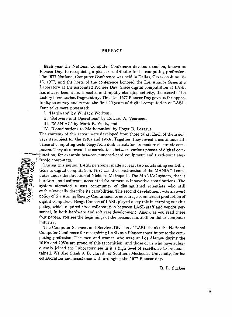
early residential and laboratory facilities. Old “TechArea 1,” where the early computers were housed,was built next to the pond, as shown in Fig. I-1. Theearly IBM accounting machines were housed in EBuilding, and the MANIAC was built in P Building.Since that time the computing center has beenmoved to South Mesa.

2. Computers in 1943

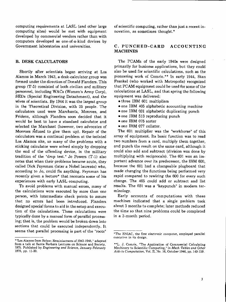
In 1943 computer technology was in an extremelyprimitive state compared to the rapidly growingneeds of nuclear research and development. Theanalog computers in use included the slide rule andthe differential analyzer. The slide rule was the ubi-quitous personal calculating device, and LASL

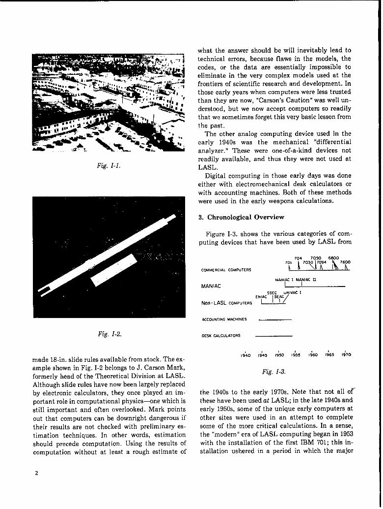
Fig. I-1.

Fig. I-2.

made 18-in. slide rules available from stock. The ex-ample shown in Fig. I-2 belongs to J. Carson Mark,formerly head of the Theoretical Division at LASL.Although slide rules have now been largely replacedby electronic calculators, they once played an im-portant role in computational physics-one which isstill important and often overlooked. Mark points

out that computers can be downright dangerous iftheir results are not checked with preliminary es-timation techniques. In other words, estimationshould precede computation. Using the results ofcomputation without at least a rough estimate of

what the answer should be will inevitably lead totechnical errors, because flaws in the models, thecodes, or the data are essentially impossible toeliminate in the very complex models used at thefrontiers of scientific research and development. Inthose early years when computers were less trustedthan they are now, “Carson’s Caution” was well un-derstood, but we now accept computers so readilythat we sometimes forget this very basic lesson fromthe past.

The other analog computing device used in theearly 1940s was the mechanical “differentialanalyzer. ” These were one-of-a-kind devices notreadily available, and thus they were not used atLASL.

Digital computing in those early days was doneeither with electromechanical desk calculators orwith accounting machines. Both of these methodswere used in the early weapons calculations.

3. Chronological Overview

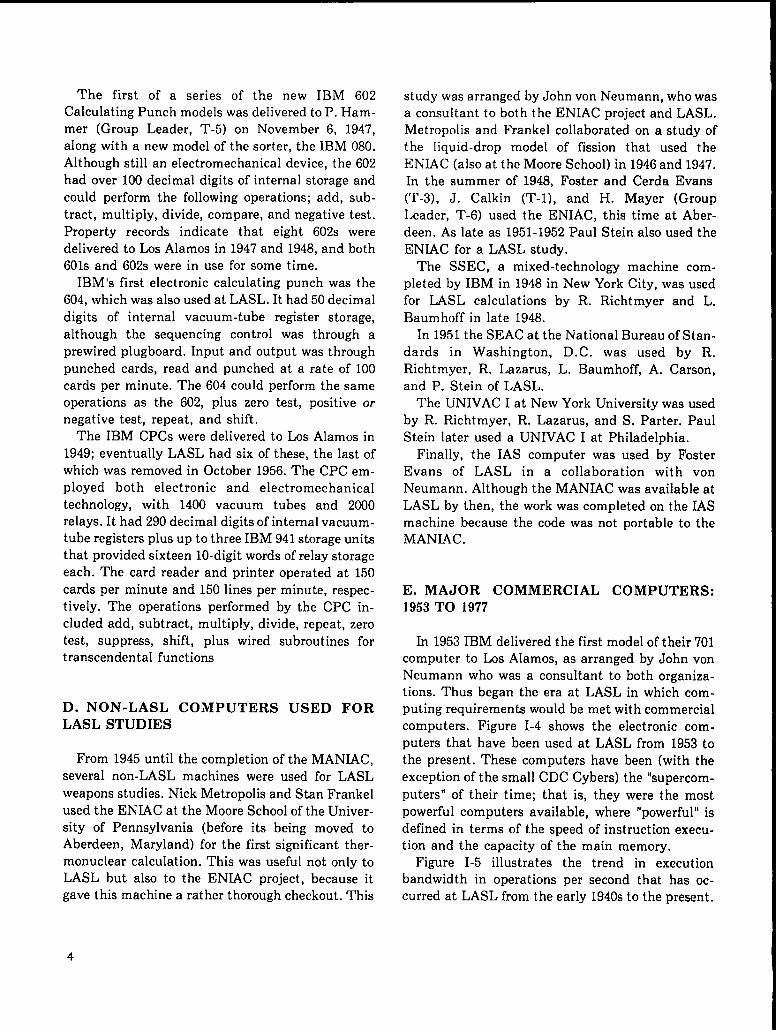
Figure I-3. shows the various categories of com-puting devices that have been used by LASL from

COMMERCIAL COMPUTERS

704 7090 6S00

‘i’ k 703N7T h ‘T

MANIAC I MANIAC U

MANIAC IISSEC uNIVAC I

Non-LASL COMPUTERS

EN\AC \SE~/

ACCOUNTING MACHINES

OESK CALCULATORS

I9:0 I9’45 IJ50 Isk I9s0 1:65 1;70

Fig. I-3.

the 1940s to the early 1970s. Note that not all orthese have been used at LASL; in the late 1940s andearly 1950s, some of the unique early computers at

other sites were used in an attempt to completesome of the more critical calculations. In a sense,the “modern” era of LASL computing began in 1953with the installation of the first IBM 701; this in-stallation ushered in a period in which the major

2

computing requirements at LASL (and other largecomputing sites) would be met with equipmentdeveloped by commercial vendors rather than withcomputers developed as one-of-a-kind devices byGovernment laboratories and universities.

B. DESK

ShortlyAlamos in .

CALCULATORS

after scientists began arriving at LosMarch 1943, a desk-calculator group was

formed under the direction of Donald Flanders. Thisgroup (T-5) consisted of both civilian and militarypersonnel, including WACS (Women’s Army Corp),SEDS (Special Engineering Detachment), and thewives of scientists. By 1944 it was the largest groupin the Theoretical Division, with 25 people. Thecalculators used were Marchants, Monroes, andFridens, although Flanders soon decided that itwould be best to have a standard calculator andselected the Marchant (however, two advocates ofMonroes &fused to give them up). Repair of thecalculators was a continual problem at the isolatedLos Alamos site, so many of the problems with asticking calculator were solved simply by droppingthe end of the offending device, in the militarytradition of the “drop test. ” Jo Powers (T-1) alsonotes that when their problems became acute, theycalled Dick Feynman (later a Nobel laureate) who,according to Jo, could fix anything. Feynman hasrecently given a lecture* that recounts some of hisexperiences with early LASL computing.

To avoid problems with manual errors, many ofthe calculations were executed by more than one

person, with intermediate check points to assurethat no errors had been introduced. Flandersdesigned specia! forms to aid in the setup and execu-tion of the calculations. These calculations weretypically done by a manual form of parallel process-ing; that is, the problem would be broken down intosections that could be executed independently. Itseems that parallel processing is part of the “roots”

—————.*“LosAlamosfromBelow:Reminiscencesof 1943-1945,”adaptedfroma talk at SantaBarbaraLectureson Scienceand Society,1975.Publishedby Engineering and Science, January-February1976,pp. 11-30.

of scientific computing, rather than just a recent in-novation, as sometimes thought. *

C. PUNCHED-CARD ACCOUNTINGIMACHINES

The PCAMS of the early 1940s were designedprimarily for business applications, but they couldalso be used for scientific calculations, such as thepioneering work of Comrie. ** In early 1944, StanFrankel (who worked with Metropolis) recognizedthat PCAM equipment could be used for some of thecalculations at LASL, and that spring the followingequipment was delivered:

● three IBM 601 multipliers● one IBM 405 alphabetic accounting machine● one IBM 031 alphabetic duplicating punch● one IBM 513 reproducing punch● one lBM 075 sorter● one IBM 077 collator.The 601 multiplier was the “workhorse” of this

array of equipment. Its basic function was to readtwo numbers from a card, multiply them together,and punch the result on the same card, although itcould also add and subtract (division was done bymultiplying with reciprocals). The 601 was an im-portant advance over its predecessor, the IBM 600,because the 601 had a changeable plugboard thatmade changing the functions being performed veryrapid compared to rewiring the 600 for every suchchange. The 405 could add or subtract and listresults. The 031 was a “keypunch” in modern ter-minology.

Early accounts of computations with thesemachines indicated that a single problem tookabout 3 months to complete; later methods reducedthe time so that nine problems could be completedin a 3-month period.

—— ———*The ENIAC,the first electroniccomputer,employedparallelexecutionin its design.

**L. J. Comrie, “The Application of CommercialCalculatingMachineryto ScientificComputing,” inMath Tables and OtherAids to Computation, Vol. II,No. 16,October1946,pp. 149-159.

The first of a series of the new IBM 602Calculating Punch models was delivered to P. Ham-mer (Group Leader, T-5) on November 6, 1947,along with a new model of the sorter, the IBM 080.Although still an electromechanical device, the 602had over 100 decimal digits of internal storage and

could perform the following operations; add, sub-tract, multiply, divide, compare, and negative test.Property records indicate that eight 602s weredelivered to Los Alamos in 1947 and 1948, and both601s and 602s were in use for some time.

IBM’s first elect ronic calculating punch was the604, which was also used at LASL. It had 50 decimal

digits of internal vacuum-tube register storage,although the sequencing control was through aprewired plugboard. Input and output was throughpunched cards, read and punched at a rate of 100cards per minute. The 604 could perform the sameoperations as the 602, plus zero test, positive or

negative test, repeat, and shift.The IBM CPCS were delivered to Los Alamos in

1949; eventually LASL had six of these, the last ofwhich was removed in October 1956. The CPC em-ployed both electronic and electromechanicaltechnology, with 1400 vacuum tubes and 2000relays. It had 290 decimal digits of internal vacuum-tube registers plus up to three IBM 941 storage unitsthat provided sixteen 10-digit words of relay storageeach. The card reader and printer operated at 150cards per minute and 150 lines per minute, respec-tively. The operations performed by the CPC in-cluded add, subtract, multiply, divide, repeat, zerotest, suppress, shift, plus wired subroutines fortranscendental functions

D. NON-LASL COMPUTERS USED FORLASL STUDIES

From 1945 until the completion of the MANIAC,several non-LASL machines were used for LASLweapons studies. Nick Metropolis and Stan Frankelused the ENIAC at the Moore School of the Univer-sity of Pennsylvania (before its being moved toAberdeen, Maryland) for the first significant ther-monuclear calculation. This was useful not only toLASL hut also to the ENIAC project, because itgave this machine a rather thorough checkout. This

study was arranged by John von Neumann, who wasa consultant to both the ENIAC project and LASL.Metropolis and Frankel collaborated on a study ofthe liquid-drop model of fission that used theENIAC (also at the Moore School) in 1946 and 1947.

In the summer of 1948, Foster and Cerda Evans(T-3), J. Calkin (T-l), and H. Mayer (GroupLeader, T-6) used the ENIAC, this time at Aber-

deen. As late as 1951-1952 Paul Stein also used theENIAC for a LASL study.

The SSEC, a mixed-technology machine com-pleted by IBM in 1948 in New York City, was usedfor LASL calculations by R. Richt myer and L.Baumhoff in late 1948.

In 1951 the SEAC at the National Bureau of Stan-dards in Washington, D.C. was used by R.Richtmyer, R. Lazarus, L. Baumhoff, A. Carson,and P. Stein of LASL.

The UNIVAC I at New York University was usedby R. Richtmyer, R. Lazarus, and S. Parter. PaulStein later used a UNIVAC I at Philadelphia.

Finally, the IAS computer was used by FosterEvans of LASL in a collaboration with vonNeumann. Although the MANIAC was available atLASL by then, the work was completed on the IASmachine because the code was not portable to theMANIAC.

E. MAJOR COMMERCIAL COMPUTERS:1953 TO 1977

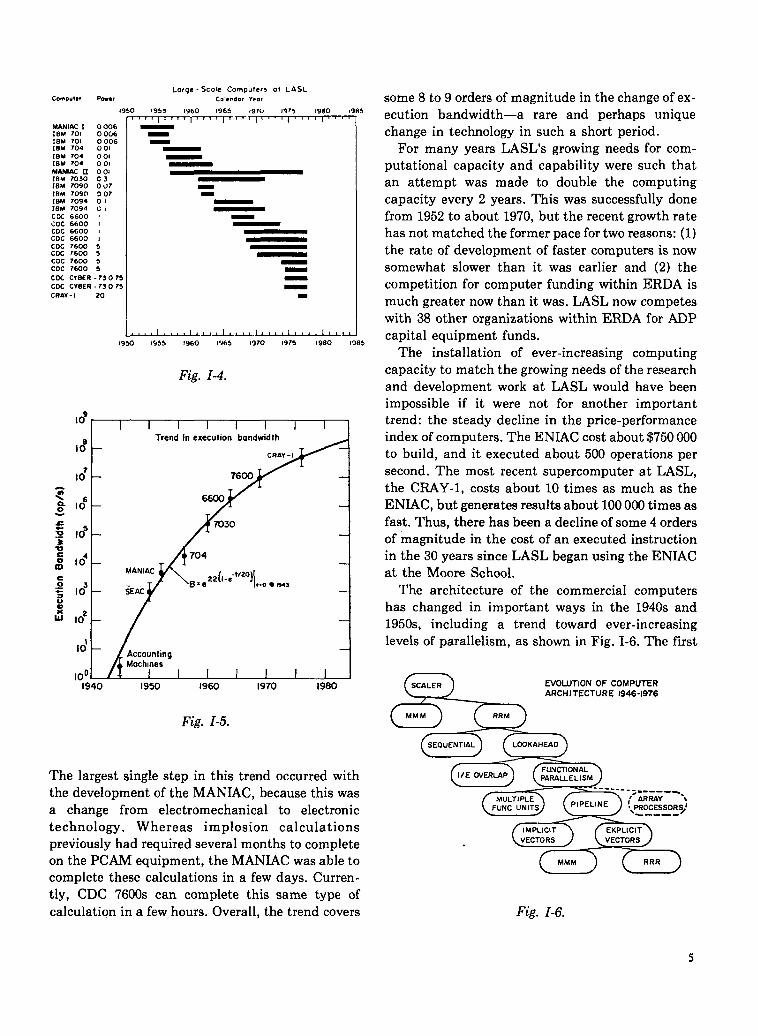
In 1953 IBM delivered the first model of their 701computer to Los Alamos, as arranged by John vonNeumann who was a consultant to both organiza-tions. Thus began the era at LASL in which com-puting requirements would be met with commercialcomputers. Figure I-4 shows the electronic com-puters that have been used at LASL from 1953 tothe present. These computers have been (with theexception of the small CDC Cybers) the “supercom-

puters” of their time; that is, they were the mostpowerful computers available, where “powerful” isdefined in terms of the speed of instruction execu-tion and the capacity of the main memory.

Figure I-5 illustrates the trend in executionbandwidth in operations per second that has oc-curred at LASL from the early 1940s to the present.

4

Ccmout.r P.m.,

19

MANIAC I 0006[EM 701 0 OC1618M 701 0006IBM 704 001IBM 704 00110M 704 001MANIAC n 004IBM 7030 03IBM 7090 007IBM 709n 90718M 7094 0 1IBM 7094 c ICCC 6600 ICDC. 6600 ICOC 6600 ICOC 6600 1COC 7600 5COC 7600 5COC 7600 5Coc 7600 5

COC CT8ER -73075COC CY8ER - ?3 O 75CRAV-I .?0

LOfq@ - Scale Computers at LASLCole”’do. Ye..

) 1957 !960 1965 1970 ,9?3 1980

~-~-

--

-

———-

-

ALLLuLL.A_LL.~1..L19X3 1555 1960 1965 1970 1975 1980 1985

Fig. I-4.

I I I I I I I ITrend In execution bandwidth

CRAV-I

7600

m

MANIAC

;EAC

AccountingMochines

100 I I I I I I1940 19s0 1960 1970 198C

Fig. I-5.

The largest single step in this trend occurred withthe development of the MANIAC, because this wasa change from electromechanical to electronictechnology. Whereas implosion calculationspreviously had required several months to completeon the PCAM equipment, the MANIAC was able tocomplete these calculations in a few days. Curren-tly, CDC 7600s can complete this same type of

calculation in a few hours. Overall, the trend covers

some 8 to 9 orders of magnitude in the change of ex-ecution bandwidth—a rare and perhaps uniquechange in technology in such a short period.

For many years LASL’S growing needs for com-putational capacity and capability were such thatan attempt was made to double the computingcapacity every 2 years. This was successfully donefrom 1952 to about 1970, but the recent growth ratehas not matched the former pace for two reasons: (1)the rate of development of faster computers is nowsomewhat slower than it was earlier and (2) thecompetition for computer funding within ERDA ismuch greater now than it was. LASL now competeswith 38 other organizations within ERDA for ADPcapital equipment funds.

The installation of ever-increasing computingcapacity to match the growing needs of the researchand development work at LASL would have beenimpossible if it were not for another importanttrend: the steady decline in the price-performanceindex of computers. The ENIAC cost about $750000to build, and it executed about 500 operations persecond. The most recent supercomputer at LASL,the CRAY-1, costs about 10 times as much as theENIAC, but generates results about 100000 times asfast. Thus, there has been a decline of some 4 ordersof magnitude in the cost of an executed instructionin the 30 years since LASL began using the ENIACat the Moore School.

The architecture of the commercial computershas changed in important ways in the 1940s and1950s, including a trend toward ever-increasinglevels of parallelism, as shown in Fig. I-6. The fiist

e!-)

--------..___~.,*’ARRAY \I\PROCESSORS,l

---—-~ ~

IMPuCIT EXPLICIT

Fig. I-6.

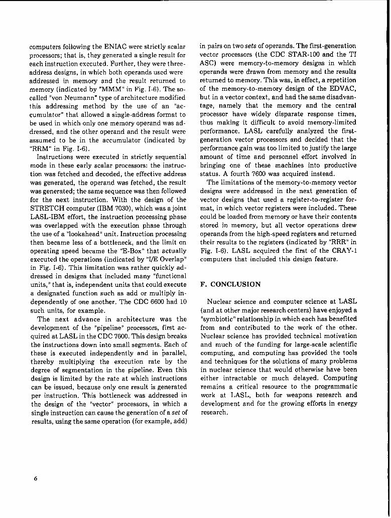
computers following the ENI.AC were strictly scalarprocessors; that is, they generated a single result foreach instruction executed. Further, they were three-address designs, in which both operands used wereaddressed in memory and the result returned tomemory (indicated by “MMM” in Fig. I-6). The so-called “von Neumann” type of architecture modifiedthis addressing met hod by the use of an “ac-cumulator” that allowed a single-address format tobe used in which only one memory operand was ad-dressed, and the other operand and the result wereassumed to be in the accumulator (indicated by“RRM” in Fig. I-6).

Instructions were executed in strictly sequentialmode in these early scalar processors: the instruc-tion was fetched and decoded, the effective addresswas generated, the operand was fetched, the resultwas generated; the same sequence was then followedfor the next instruction. With the design of theSTRETCH computer (IBM 7030), which was a jointLASL-IBM effort, the instruction processing phasewas overlapped with the execution phase throughthe use of a “lookahead” unit. Instruction processingthen became less of a bottleneck, and the limit onoperating speed became the “E-Box” that actuallyexecuted the operations (indicated by “VIZ Overlap”in Fig. I-6). This limitation was rather quickly ad-dressed in designs that included many “functionalunits, ” that is, independent units that could executea designated function such as add or multiply in-dependently of one another. The CDC 6600 had 10such units, for example.

The next advance in architecture was thedevelopment of the “pipeline” processors, first ac-quired at LASL in the CDC 7600. This design breaksthe instructions down into small segments. Each ofthese is executed independently and in ~arallel,thereby multiplying the execution rate by thedegree of segmentation in the pipeline. Even thisdesign is limited by the rate at which instructionscan be issued, because only one result is generatedper instruction. This bottleneck was addressed inthe design of the “vector” processors, in which a

single instruction can cause the generation of a set ofresults, using the same operation (for example, add)

in pairs on two sets of operands. The first-generationvector processors (the CDC STAR-1OO and the TIASC) were memory-to-memory designs in whichoperands were drawn from memory and the resultsreturned to memory. This was, in effect, a repetitionof the memory-to-memory design of the EDVAC,but in a vector context, and had the same disadvan-tage, namely that the memory and the centralprocessor have widely disparate response times,thus making it difficult to avoid memory-limitedperformance. LASL carefully analyzed the first-generation vector processors and decided that theperformance gain was too limited to justify the largeamount of time and personnel effort involved inbringing one of these machines into productivestatus. A fourth 7600 was acquired instead.

The limitations of the memory-to-memory vectordesigns were addressed in the next generation ofvector designs that used a register-to-register for-mat, in which vector registers were included. Thesecould be loaded from memory or have their contentsstored in memory, but all vector operations drewoperands from the high-speed registers and returnedtheir results to the registers (indicated by “RRR” inFig. I-6). LASL acquired the first of the CRAY-1computers that included this design feature.

F. CONCLUSION

Nuclear science and computer science at LASL

(and at other major research centers) have enjoyed a“symbiotic” relationship in which each has benefitedfrom and contributed to the work of the other.Nuclear science has provided technical motivationand much of the funding for large-scale scientificcomputing, and computing has provided the toolsand techniques for the solutions of many problemsin nuclear science that would otherwise have beeneither intractable or much delayed. Computingremains a critical resource to the programmaticwork at LASL, both for weapons research anddevelopment and for the growing efforts in energyresearch.

6

11SOFTWARE AND OPERATIONS

by

Edward A.

A. INTRODUCTION

A more descriptive title would be “Software withNotes on Programming and Operations, ” becauseduring the 1940s and 1950s, the coder (today called aProgrammer or Systems Analyst) was usually theoperator as well. Scientists normally programmedtheir own applications codes and on occasion mightalso code utility programs such as a card loadingroutine. They primarily used longhand, or machinelanguage, in the larger codes to minimize runningtime. They were not afraid of “getting their handsdirty” and would do almost any related task to ac-complish the primary work of math, physics, or anyother field in which they were engaged. Some of thishistory was not well documented, “and many of theold write-ups are not dated. Some details thereforecould be slightly in error. I hope to convey a feelingfor how computing was done in the “good old days”as well as to provide some information on thehardware and software available then.*

Hand computing was performed in the 1940sthrough the mid-1950s. At its peak there wereperhaps 20 to 30 people using Marchant and Fridendesk calculators. Mathematicians and physicistswould partition the functions to be calculated intosmall calculational steps. These, functions generallyrequired many iterations and/or the varying of the

parameter values. In many respects this constitutedprogramming by the scientists for a “computer” thatconsisted of one or more humans doing thecalculating, following a set of step-by-step “instruc-tions. ”

The computing machines at LASL in the 1940sand 1950s fell into four groups. From 1949 to 1956,LASL used IBM CPCS; from 1953 through 1956,IBM 701s were also installed. These were allreplaced almost overnight in 1956 by three 704s,—_————*I will discussLASL’Seffort primarily,and referencesto IBMusuallywillbe to indicatea joint effortor to maintaina frameofhistoricalreference.

Voorhees

which remained until 1961. The IBM STRETCHcomputer arrived in 1961, but there was a period

before that of about 5 years during which LASL diddevelopment work on both the hardware andsoftware in cooperation with IBM.

B. CARD-PROGRAMMED CALCULATORERA

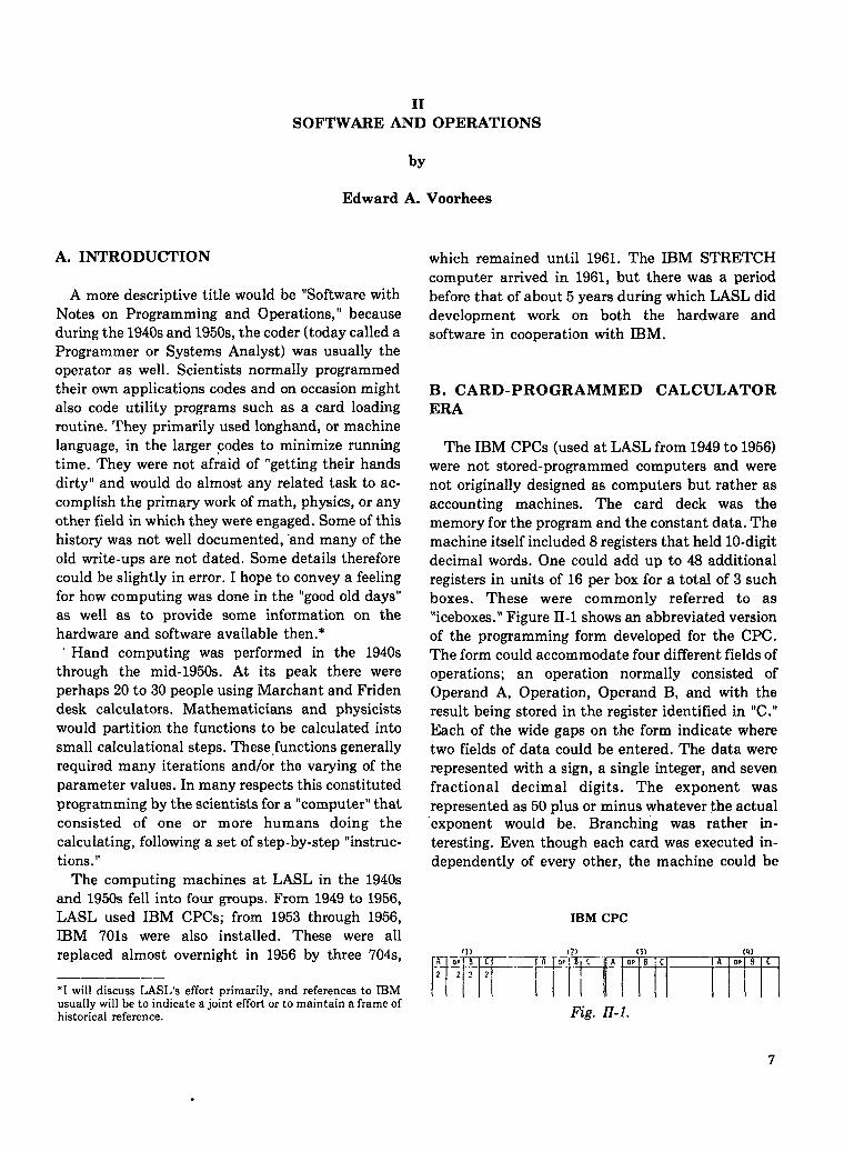
The IBM CPCS (used at LASL from 1949 to 1956)were not stored-programmed computers and werenot originally designed as computers but rather asaccounting machines. The card deck was thememory for the program and the constant data. Themachine itself included 8 registers that held 10-digitdecimal words. One could add up to 48 additionalregisters in units of 16 per box for a total of 3 suchboxes. These were commonly referred to as“iceboxes.” Figure II-1 shows an abbreviated versionof the programming form developed for the CPC.The form could accommodate four different fields ofoperations; an operation normally consisted ofOperand A, Operation, Operand B, and with theresult being stored in the register identified in “C.”Each of the wide gaps on the form indicate wheretwo fields of data could be entered. The data wererepresented with a sign, a single integer, and sevenfractional decimal digits. The exponent wasrepresented as 50 plus or minus whatever the actual“exponent would be. Branching was rather in-teresting. Even though each card was executed in-dependently of every other, the machine could be

IBM CPC

<1) {2) (n (4)

l-TTl-F7TlTii’”0’‘Ic A0’‘cFig. ZZ-1.

.

programmed to remember which of the four fields ofoperations it was following at any given time.Therefore, if the program had a branch (either un-conditional or conditional) among the instructionsin field 1, the machine could begin to execute itsnext instruction from any one of the other threefields. In this way you could branch between fieldsand follow a different sequence of instructions.

The design and use of the wired board “created” ageneral purpose floating-decimal computer from anaccounting machine. The F Control Panels wereLASL’S most advanced wired boards and had manyof the elements of “macrocoding.”

Figure II-2 shows some of the operations thatcould be performed from a single card using the F

Control Panels. Note that in these cases there aretwo operands and one result with a third operand,X, coming from another field of the form. Usually,

CPC SINGLE-CARD OPERATION EXAMPLES

A+ B+X+C

Bit)( -c

A

(A+ B)*X+C

xAuB

+C

Fig. II-2.

these operations could be executed in one card cy-cle. Some of them would take longer than one cycle,so the programmer would have to put a blank cardin the deck to give the machine enough time to ex-ecute that instruction before proceeding to the nextone.

Figure II-3 shows some of the functions that wereavailable on the CPC. The functions here and theoperations in Fig. II-2 resemble modern-day sub-routines, but they were subprograms wired on the

board. Some of them were fairly complex, and oftenblank cards were again necessary to provide enoughtime for the CPC to execute the function.

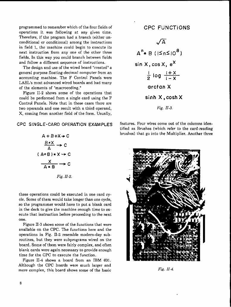
Figure II-4 shows a board from an IBM 601.Although the CPC boards were much larger andmore complex, this board shows some of the basic

CPC FUNCTIONS

n

A“* B (/<nSJ08)

sin X, COSX) ex

features.tified asbrushes)

~ log ++

arctan X

sinh X ,cosh X

Fig. II-3.

Four wires come out of the columns iden-Brushes (which refer to the card-readingthat go into the Multiplier. Another three

Fig. II-4.

8

wires go into the Multiplicand, and the Product isrouted to the Card Punch. There were a total of six

CPCS at LASL; the last one did not leave until latein 1956, well after the three 701s had already depar-ted and three 704s had been installed.

The operator would stand in front of the machine,recycle the cards for hours, perhaps change to alter-nate decks of cards, watch the listing, and often“react.” In other words, over 25 years ago we alreadyhad “interactive computing.”

C. IBM 701 ERA

The IBM 701 originally was announced as the“Defense Calculator. ” LASL was the recipient of the

serial number 1 machine, which arrived in April1953 and remained until the fall of 1956. A second701 calculator, as it was later called, came inFebruary 1954. The machine was fixed binary. Allnumbers were assumed to be less than one; that is,the binary point was on the extreme left of the num-ber. The electrostatic storage (which was not tooreliable) could hold 2046 36-bit full words or 409616-bit half-words. It was possible later to double thesize of that memory, which LASL did indeed do. In-structions were all half-words; data could also be inhalf-word format. Instructions were single addresswith no indexing. There was no parallel 1/0. Thesystem consisted of one card reader, one printer, onememory drum storage unit, two tape drives (whichoften did not work), and one card punch (theprimary device for machine-readable output).

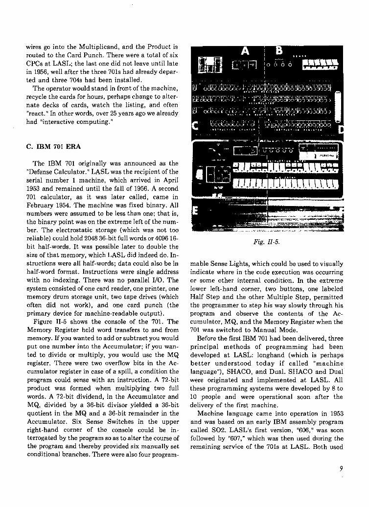
Figure II-5 shows the console of the 701. TheMemory Register held word transfers to and frommemory. If you wanted to add or subtract you wouldput one number into the Accumulator; if you wan-ted to divide or multiply, you would use the MQregister. There were two overflow bits in the Ac-cumulator register in case of a spill, a condition theprogram could sense with an instruction. A 72-bitproduct was formed when multiplying two fullwords. A 72-bit dividend, in the Accumulator andMQ, divided by a 36-bit divisor yielded a 36-bitquotient in the MQ and a 36-bit remainder in theAccumulator. Six Sense Switches in the upperright-hand corner of the console could be in-terrogated by the program so as to alter the course ofthe program and thereby provided six manually setconditional branches. There were also four program-

Fig. II-5.

mable Sense Lights, which could be used to visuallyindicate where in the code execution was occurringor some other internal condition. In the extremelower left-hand corner, two buttons, one labeledHalf Step and the other Multiple Step, permittedthe programmer to step his way slowly through hisprogram and observe the contents of the Ac-cumulator, MQ, and the Memory Register when the701 was switched to Manual Mode.

Before the first IBM 701 had been delivered, threeprincipal methods of programming had beendeveloped at LASL: longhand (which is perhapsbetter understood today if called “machinelanguage”), SHACO, and Dual. SHACO and Dualwere originated and implemented at LASL. Allthese programming systems were developed by 8 to10 people and were operational soon after thedelivery of the first machine,

Machine language came into operation in 1953and was based on an early IBM assembly programcalled S02. LASL’S first version, “606,” was soonfollowed by “607,” which was then used during theremaining service of the 701s at LASL. Both used

9

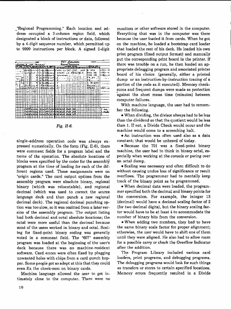
_“Regional Programming.” Each location and ad-dress occupied a 3-column region field, whichdesignated a block of instructions or data, followedby a 4-digit sequence number, which permitted upto 9999 instructions per block. A signed 2-digit

w_—- can’. 70 f edd;% ,,W. _—

Fig. II-6.

single-address operation code was always ex-pressed numerically. On the form (Fig. II-6), therewere comment fields for a program label and thename of the operation. The absolute locations ofblocks were specified by the coder for the assembl~program at the time of loading for each of the dif-ferent regions used. These assignments were on

“origin cards.” The card output options from theassembly program were absolute binary, regionalbinary (which was relocatable), and regionaldecimal (which was used to correct the sourcelanguage deck and then punch a new regionaldecimal deck). The regional decimal punching op-tion was too slow, so it was omitted from a later ver-sion of the assembly program. The output listinghad both decimal and octal absolute locations; theoctal were more useful than the decimal becausemost of the users worked in binary and octal. Scal-ing for fixed-point binary coding was generallynoted in a comment field. The “607” assemblyprogram was loaded at the beginning of the user’sdeck because there was no machine-residentsoftware. Card errors were often fixed by pluggingunwanted holes with chips from a card punch hop-per. Some people got so adept at this that they couldeven fix the check-sum on binary cards.

Machine language allowed the user to get in-timately close to the computer. There were no

monitors or other software stored in the computer.Everything that was in the computer was therebecause the user loaded it from cards. When he goton the machine, he loaded a bootstrap card loaderthat loaded the rest of his deck. He loaded his ownprint program (fixed output format) and manually

put the corresponding print board in the printer. Ifthere was trouble on a run, he then loaded an ap-propriate debugging program and associated printerboard of his choice (generally, either a printeddump or an instruction-by-instruction tracing of aportion of the Fode as it executed). Memory check-~ums and frequent dumps were made as protectionagainst the short mean time (minutes) betweencomputer failures.

With machine language, the user had to remem-ber the following.

● When dividing, the divisor always had to be less

than the dividend so that the quotient would be lessthan 1. If not, a Divide Check would occur and themachine would come to a screeching halt.

● An instruction was often used also as a dataconstant; that would be unheard of today.

● Because the 701 was a fixed-point binarymachine, the user had to think in binary octal, es-pecially when working at the console or poring overan octal dump.

. Scaling was necessary and often difficult to dowithout causing undue loss of significance or resultoverflows. The programmer had to mentally keeptrack of the binary point as he programmed.

● When decimal data were loaded, the program-mer specified both the decimal and binary points for

the conversion. For example, the integer 13(decimal) would have a decimal scaling factor of 2(for two decimal digits), but the binary scaling fac-tor would have to be at least 4 to accommodate thenumber of binary bits from the conversion.

. When adding two numbers, they had to havethe same binary scale factor for proper alignment;otherwise, the user would have to shift one of themuntil they were aligned. He also had to allow roomfor a possible carry or check the Overflow Indicatorafter the addition.

The Program Library included various cardloaders, print programs, and debugging programs.The debugging programs would look for such thingsas transfers or stores to certain specified locations.

Memory errors frequently resulted in a Divide

10

Check and a machine stop, Occasionally, instruc-tion sequence control would be lost, and a jumpwould occur to some part of memory where it shouldnot be. In this case, when the machine stopped youhad no idea how control got to that location.

LASL Group T-1, which ran the computer opera-tion, began issuing materials and offering program-ming classes in 1953. At that time there were about80 users outside of T-1. By August, LASL wasalready operating 24 hours per day. Six 701s hadbeen delivered nationwide by then, and there wasenough interest among users to hold a program-exchange meeting at Douglass Aircraft (SantaMonica). This meeting was the forerunner of theSHARE organization formed in 1955 of which LASLwas a charter member.

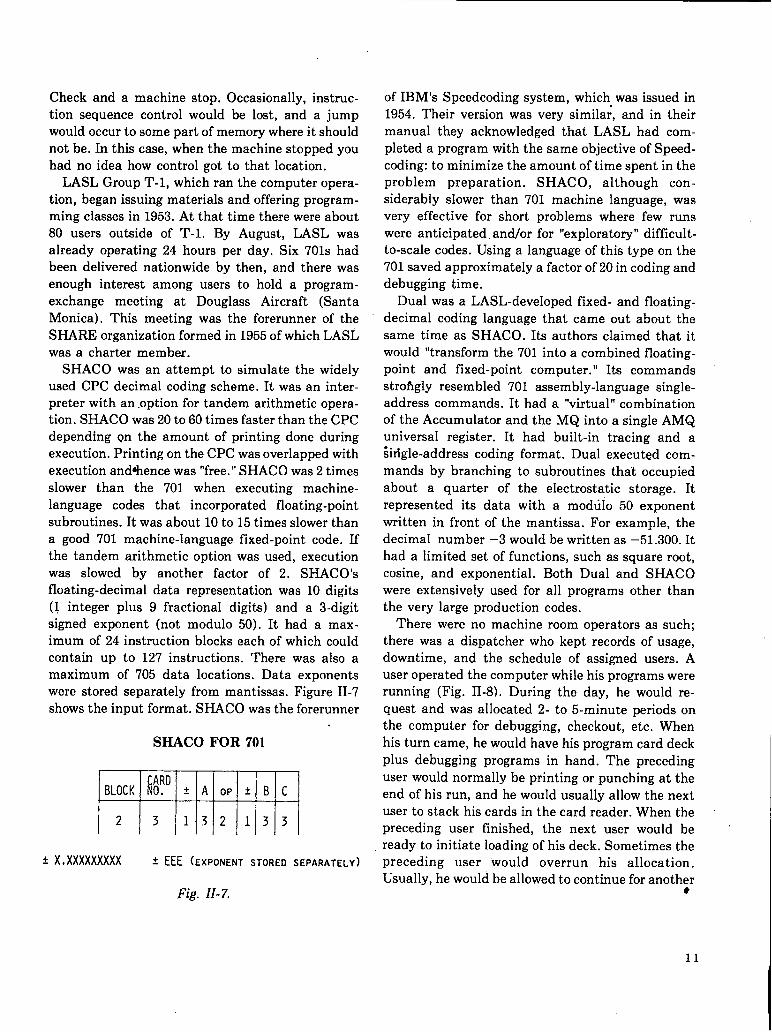
SHACO was an attempt to simulate the widelyused CPC decimal coding scheme. It was an inter-preter with an option for tandem arithmetic opera-tion. SHACO was 20 to 60 times faster than the CPCdepending on the amount of printing done duringexecution. Printing on the CPC was overlapped withexecution and~hence was “free.” SHACO was 2 timesslower than the 701 when executing machine-language codes that incorporated floating-pointsubroutines. It was about 10 to 15 times slower thana good 701 machine-language fixed-point code. Ifthe tandem arithmetic option was used, executionwas slowed by another factor of 2. SHACO’Sfloating-decimal data representation was 10 digits(1 integer plus 9 fractional digits) and a 3-digitsigned exponent (not modulo 50). It had a max-imum of 24 instruction blocks each of which couldcontain up to 127 instructions. There was also amaximum of 705 data locations. Data exponentswere stored separately from mantissas. Figure II-7shows the input format. SHACO was the forerunner

SHACO FOR 701

mL x , Xxxxxxxxx * EEE (EXPONENT STORED SEPARATELY)

Fig. II-7.

of IBM’s Speedcoding system, which was issued in1954. Their version was very simila~, and in theirmanual they acknowledged that LASL had com-pleted a program with the same objective of Speed-coding: to minimize the amount of time spent in theproblem preparation. SHACO, although con-siderably slower than 701 machine language, wasvery effective for short problems where few runswere anticipated, and/or for “exploratory” difficult-to-scale codes. Using a language of this type on the701 saved approximately a factor of 20 in coding anddebugging time.

Dual was a LASL-developed fixed- and floating-decimal coding language that came out about thesame time as SHACO. Its authors claimed that itwould “transform the 701 into a combined floating-point and fixed-point computer. ” Its commandsstrofigly resembled 701 assembly-language single-address commands. It had a “virtual” combinationof the Accumulator and the MQ into a single AMQuniversal register. It had built-in tracing and a;irigle-address coding format. Dual executed com-mands by branching to subroutines that occupiedabout a quarter of the electrostatic storage. Itrepresented its data with a modulo 50 exponentwritten in front of the mantissa. For example, thedecimal number –3 would be written as –51.300. Ithad a limited set of functions, such as square root,cosine, and exponential. Both Dual and SHACOwere extensively used for all programs other thanthe very large production codes.

There were no machine room operators as such;there was a dispatcher who kept records of usage,downtime, and the schedule of assigned users. Auser operated the computer while his programs wererunning (Fig. II-8). During the day, he would re-

quest and was allocated 2- to 5-minute periods onthe computer for debugging, checkout, etc. Whenhis turn came, he would have his program card deck

plus debugging programs in hand. The precedinguser would normally be printing or punching at theend of his run, and he would usually allow the nextuser to stack his cards in the card reader. When thepreceding user finished, the next user would beready to initiate loading of his deck. Sometimes thepreceding user would overrun his allocation.Usually, he would be allowed to continue for anoth~r

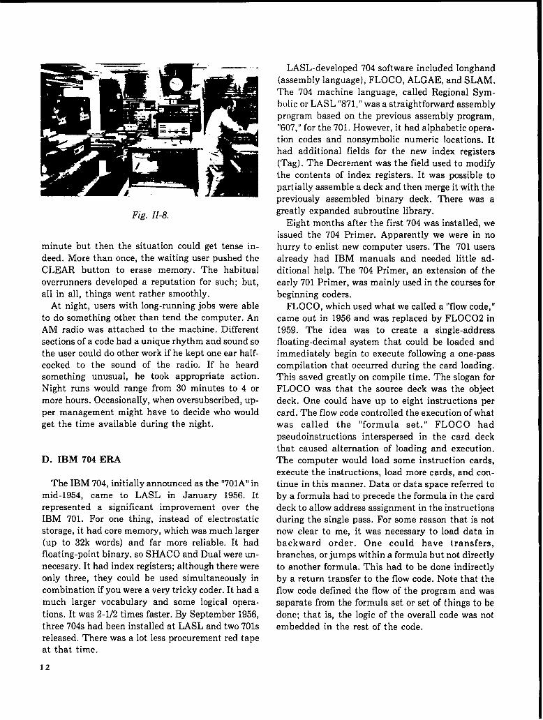
Fig. II-8.

minute but then the situation could get tense in-deed. More than once, thewait.ing user pushed theCLEAR button to erase memory. The habitualoverrunners developed a reputation for such; but,all in all, things went rather smoothly.

At night, users with long-running jobs were ableto do something other than tend the computer. AnAM radio was attached to the machine. Differentsections of a code had a unique rhythm and sound sothe user could do other work if he kept one ear half-cocked to the sound of the radio. If he heardsomething unusual, he took appropriate action.Night runs would range from 30 minutes to 4 ormore hours. Occasionally, when oversubscribed, up-per management might have to decide who wouldget the time available during the night.

D. IBM 704 ERA

The IBM 704, initially announced as the “701A” inmid-1954, came to LASL in January 1956. Itrepresented a significant improvement over theIBM 701. For one thing, instead of electrostaticstorage, it had core memory, which was much larger(up to 32k words) and far more reliable. It hadfloating-point binary, so SHACO and Dual were un-necessary. It had index registers; although there wereonly three, they could be used simultaneously incombination if you were a very tricky coder. It had amuch larger vocabulary and some logical opera-

tions. It was 2-1/2 times faster. By September 1956,three 704s had been installed at LASL and two 701sreleased. There was a lot less procurement red tapeat that time.

12

LASL-developed 704 software included longhand(assembly language), FLOCO, ALGAE, and SLAM.The 704 machine language, called Regional Sym-bolic or LASL “871,” was a straightforward assemblyprogram based on the previous assembly program,“607,” for the 701. However, it had alphabetic opera-tion codes and nonsymbolic numeric locations. Ithad additional fields for the new index registers(Tag). The Decrement was the field used to modifythe contents of index registers. It was possible topartially assemble a deck and then merge it with thepreviously assembled binary deck. There was agreatly expanded subroutine library.

Eight months after the first 704 was installed, weissued the 704 Primer. Apparently we were in nohurry to enlist new computer users. The 701 usersalready had IBM manuals and needed little ad-ditional help. The 704 Primer, an extension of theearly 701 Primer, was mainly used in the courses forbeginning coders.

FLOCO, which used what we called a “flow code, ”came out in 1956 and was replaced by FLOC02 in1959. The idea was to create a single-addressfloating-decimal system that could be loaded andimmediately begin to execute following a one-passcompilation that occurred during the card loading.This saved greatly on compile time. The slogan forFLOCO was that the source deck was the objectdeck. One could have up to eight instructions percard. The flow code controlled the execution of whatwas called the “formula set. ” FLOCO had

pseudoinstructions interspersed in the card deckthat caused alternation of loading and execution.The computer would load some instruction cards,execute the instructions, load more cards, and con-tinue in this manner. Data or data space referred toby a formula had to precede the formula in the carddeck to allow address assignment in the instructionsduring the single pass. For some reason that is notnow clear to me, it was necessary to load data inbackward order. One could have transfers,branches, or jumps within a formula but not directlyto another formula. This had to be done indirectlyby a return transfer to the flow code. Note that theflow code defined the flow of the program and was

separate from the formula set or set of things to bedone; that is, the logic of the overall code was notembedded in the rest of the code.

!In 1958, the ALGAE language was implemented

at LASL for the 704. It was a preprocessor to FOR-

TRAN (which was first issued by IBM in 1957). Thelanguage contained a control structure that resem-

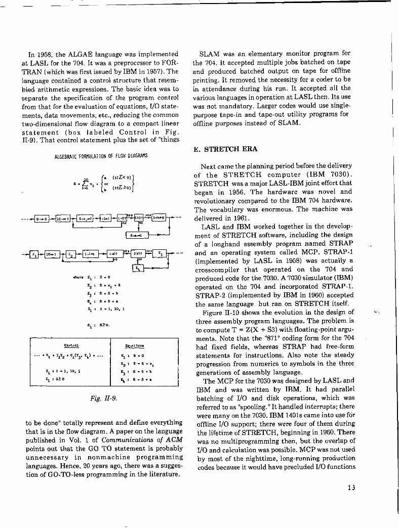
bled arithmetic expressions. The basic idea was toseparate the specification of the program controlfrom that for the evaluation of equations, 1/0 state-ments, data movements, etc., reducing the commontwo-dimensional flow diagram to a compact linearstatement (box labeled Control in Fig.II-9). That control statement plus the set of “things

SLAM was an elementary monitor program forthe 704. It accepted multiple jobs batched on tapeand produced batched output on tape for offline

printing. It removed the necessity for a coder to bein attendance during his run. It accepted all thevarious languages in operation at LASL then. Its usewas not mandatory. Larger codes would use single-purpose tape-in and tape-out utility programs foroffline purposes instead of SLAM.

E. STRETCH ERAALGEBRAICFOFUWAT10N OF FLON DlAWINS

o-s lC- 1 S.X -s---

I

.

where \: S-O

E2: S.xi+s

5 : S-S. b

% : S. S+*

\ti . 1, 10, 1

Control ?a!M?!E.. . +rl ● x1t2+ C1(E3,z,) + . . . ~: s-o

C2! S.s+xi

1111 -1,10,1 E3!S-S+b

c1 1s20 ~1 s-s+,

Fig. 11-9.

to be done” totally represent and defiie everythingthat is in the flow diagram. A paper on the languagepublished in Vol. 1 of Communications of ACM

points out that the GO TO statement is probablyunnecessary in nonmachine programminglanguages. Hence, 20 years ago, there was a sugges-tion of GO-TO-less programming in the literature.

Next came the planning period before the delivery

of the STRETCH computer (IBM 7030).STRETCH was a major LASL-IBM joint effort thatbegan in 1956. The hardware was novel andrevolutionary compared to the IBM 704 hardware.The vocabulary was enormous. The machine wasdelivered in 1961.

LASL and lBM worked together in the develop-ment of STRETCH software, including the design

of a longhand assembly program named STRAPand an operating system called MCP. STRAP-1(implemented by LASL in 1958) was actually acrosscompiler that operated on the 704 andproduced code for the 7030. A 7030 simulator (IBM)operated on the 704 and incorporated STRAP-1.STRAP-2 (irnplernented by IBM in 1960) acceptedthe same language but ran on STRETCH itself.

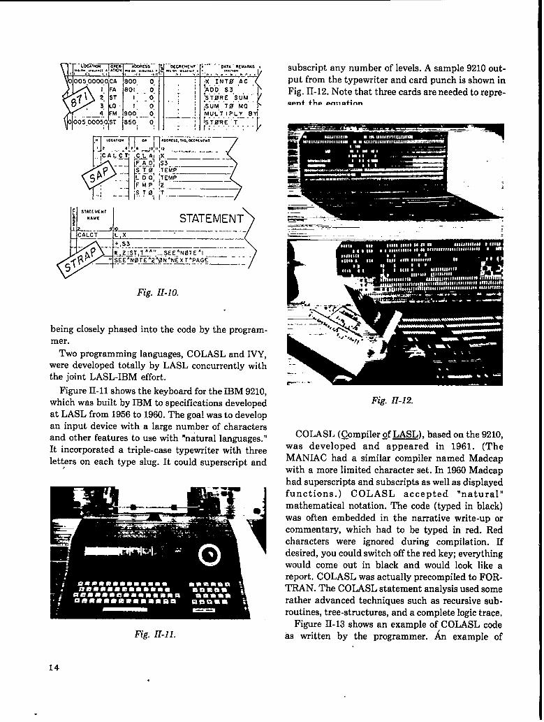
Figure II-10 shows the evolution in the design of =-three assembly program languages. The problem isto compute T = Z(X + S3) with floating-point argu-ments. Note that the “871” coding form for the 704had fixed fields, whereas STRAP had free-formstatements for instructions. Also note the steadyprogression from numerics to symbols in the threegenerations of assembly language.

The MCP for the 7030 was designed by LASL andIBM and was written by IBM. It had parallelbatching of 1/0 and disk operations, which wasreferred to as “spooling.” It handled interrupts; therewere many on the 7030. IBM 1401s came into use foroffline I/O support; there were four of them during

the lifetime of STRETCH, beginning in 1960. Therewas no multiprogramming then, but the overlap of

I/O and calculation was possible. MCP was not usedby most of the nighttime, long-running productioncodes because it would have precluded 1/0 functions

13 I

yjijJ’-~ml’ ~me.. ,,.,,.,, . Anw ,,..0 ,, O”, W, , ,,’0. .G.MM , , 0 ,,.,! .0..

1:C/,

F+J ::1.,, . !—..—. ——

-;-— is‘gi tT- --— /

Fig. II-10.

being closely phased into the code by the program-mer.

Two programming languages, COLASL and IVY,were developed totally by LASL concurrently withthe joint LASL-IBM effort.

Figure II-II shows the keyboard for the IBM 9210,which was built by IBM to specifications developedat LASL from 1956 to 1960. The goal was to developan input device with a large number of charactersand other features to use with “natural languages. ”It incorporated a triple-case typewriter with threeletters on each type slug. It could superscript and,

Fig. II-11,

subscript any number of levels. A sample 9210 out-put from the typewriter and card punch is shown inFig. II-12. Note that three cards are needed to repre-wmt tho aallaticnm

,- _——.—— —=. .-.-. ,.,— ;

Fig. ZI-12.

COLASL (Qompiler of LASL), based on the 9210,was developed and appeared in 1961. (TheMANIAC had a similar compiler named Madcapwith a more limited character set. In 1960 Madcaphad superscripts and subscripts as well as displayedfunctions. ) COLASL accepted “natural”mathematical notation. The code (typed in black)

was often embedded in the narrative write-up orcommentary, which had to be typed in red. Redcharacters were ignored during compilation. Ifdesired, you could switch off the red key; everythingwould come out in black and would look like areport. COLASL was actually precompiled to FOR-TRAN. The COLASL statement analysis used somerather advanced techniques such as recursive sub-routines, tree-structures, and a complete logic trace,

Figure II-13 shows an example of, COLASL codeas written by the programmer. An example of

14.

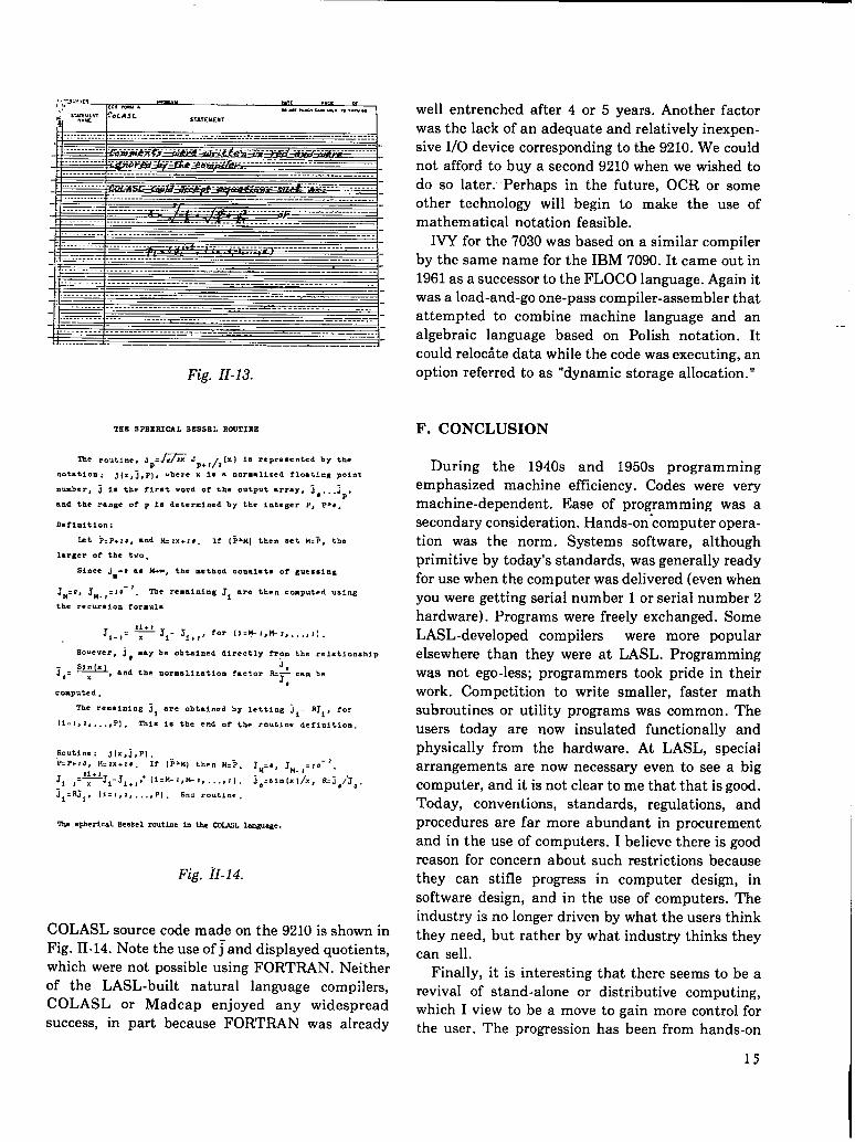
Fig. II-13.

lW8 SPIII!RICAL BSSSBL llOUTIXll

~e routine, .tp.~ Jp+,/,(x) i. represented by the

nOta*lOn: J fx, ~, PI, where x 1* u nOr=allz=d f10atin8 pOint

number, j is the first word of the output array, j, . . . .P’

end the ran~e of p is determirmd by the integer P, P*#.

Definition:

Let P, P+, o, and I& ,x+,,. If (=>M) then set k~, the

larger of the two.

Since Jm-o as U-W, the method connistn of Iwessing

JM.O, J“.,.l a-’. The remr.lning .Ti are then computed using

the recursion formula

Ji-l= *Ti- J,+,, for [i. M- I,t4-z, . . .. I].

Hov-=r, ~, may be obtained directly from the relationship

3~o- Sln(xlx

, and the wc.rnallzation factor R=l can beJo

computed .

Tbe remaining ji are obtal”ed by letting ji: RJi, for

(1.1, 2,. ... P]. TM. is the ●nd of the routim definition

Routi..: J(x, ~.pl.?= P+ IO, t4,2x+ 1*. If (;WI then k;. rM. *, JM. ,=1 O-’.

r 1- I .~rl-~i+ , ,“ (l= M- I>~Z>. ... II. j@= Sfn(X )/X, R=j,/’Jo.

Ji=RIf, li=I)Z, . . ..pl. End routine .

The S@Iericd. Seskel mtIne in the COLAsLLmgu=e.

Fig. II-14.

COLASL source code made on the 9210 is shown inFig. II-14. Note the use of ~and displayed quotients,which were not possible using FORTRAN. Neitherof the LASL-built natural language compilers,COLASL or Madcap enjoyed any widespreadsuccess, in part because FORTRAN was already

well entrenched after 4 or 5 years. Another factorwas the lack of an adequate and relatively inexpen-sive 1/0 device corresponding to the 9210. We couldnot afford to buy a second 9210 when we wished todo so later. Perhaps in the future, OCR or someother technology will begin to make the use ofmathematical notation feasible.

IVY for the 7030 was based on a similar compilerby the same name for the IBM 7090. It came out in1961 as a successor to the FLOCO language. Again itwas a load-and-go one-pass compiler-assembler thatattempted to combine machine language and analgebraic language based on Polish notation. Itcould relocate data while the code was executing, anoption referred to as “dynamic storage allocation. ”

F. CONCLUSION

During the 1940s and 1950s programmingemphasized machine efficiency. Codes were verymachine-dependent. Ease of programming was asecondary consideration. Hands-on.computer opera-tion was the norm. Systems software, althoughprimitive by today’s standards, was generally readyfor use when the computer was delivered (even whenyou were getting serial number 1 or serial number 2hardware). Programs were freely exchanged. SomeLASL-developed compilers were more popularelsewhere than they were at LASL. Programmingwas not ego-less; programmers took pride in theirwork. Competition to write smaller, faster mathsubroutines or utility programs was common. Theusers today are now insulated functionally andphysically from the hardware. At LASL, specialarrangements are now necessary even to see a bigcomputer, and it is not clear to me that that is good.Today, conventions, standards, regulations, andprocedures are far more abundant in procurementand in the use of computers. I believe there is goodreason for concern about such restrictions becausethey can stifle progress in computer design, insoftware design, and in the use of computers. Theindustry is no longer driven by what the users thinkthey need, but rather by what industry thinks theycan sell.

Finally, it is interesting that there seems to be arevival of stand-alone or distributive computing,which I view to be a move to gain more control forthe user. The progression has been from hands-on

15

computing with optilhization of hardware utiliza - The trend now seems headed back toward increasedtion to batch (no hands-on) to timesharing (pseudo interest in efficient hardware utilization.hands-on with no concern for hardware efficiency).

IIIMANIAC

by

Mark B. Wells

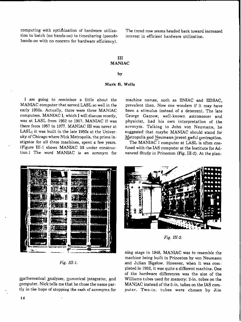
I am going to reminisce a little about theMANIAC computer that served LASL so well in theearly 1950s. Actually, there were three MANIACcomputers. MANIAC I, which I will discuss mostly,was at LASL from 1952 to 1957. MANIAC II wasthere from 1957 to 1977. MANIAC III was never atLASL; it was built in the late 1950s at the Univer-sity of Chicago where Nick Metropolis, the prime in-stigator for all three machines, spent a few years.

(Figure III- 1 shows MANIAC I.11under construc-tion. ) The word MANIAC is an acronym for

machine names, such as ENIAC and EDSAC,

prevalent then. Now one wonders if it may havebeen a stimulus instead of a deterrent. The lateGeorge Gamow, well-known astronomer andphysicist, had his own interpretation of theacronym. Talking to John von Neumann, hesuggested that maybe MANIAC should stand for

Metropolis gnd ~eumann &vent ~wful gontrapt ion.The MANIAC I computer at LASL is often con-

fused with the I&S computer at the Institute for Ad-vanced Study in Princeton (Fig. HI-2). At the plan-

Fig. III-1.

~athematical Analyzer, ~umerical @tegrator, ~nd

Somputer. Nick tells me that he chose the name par-

. . tly in the hope of stopping the rash of acronyms for

16

Fig. III-2.

ning stage in 1948, MANIAC was to resemble themachine being built in Princeton by von Neumannand Julian Bigelow. However, when it was com-pleted in 1952, it was quite a different machine. Oneof the hardware differences was the size of theWilliams tubes used for memory: 2-in, tubes on the

MANIAC instead of the 5-in. tubes on the IAS com-puter. Two-in. tubes were chosen by Jim

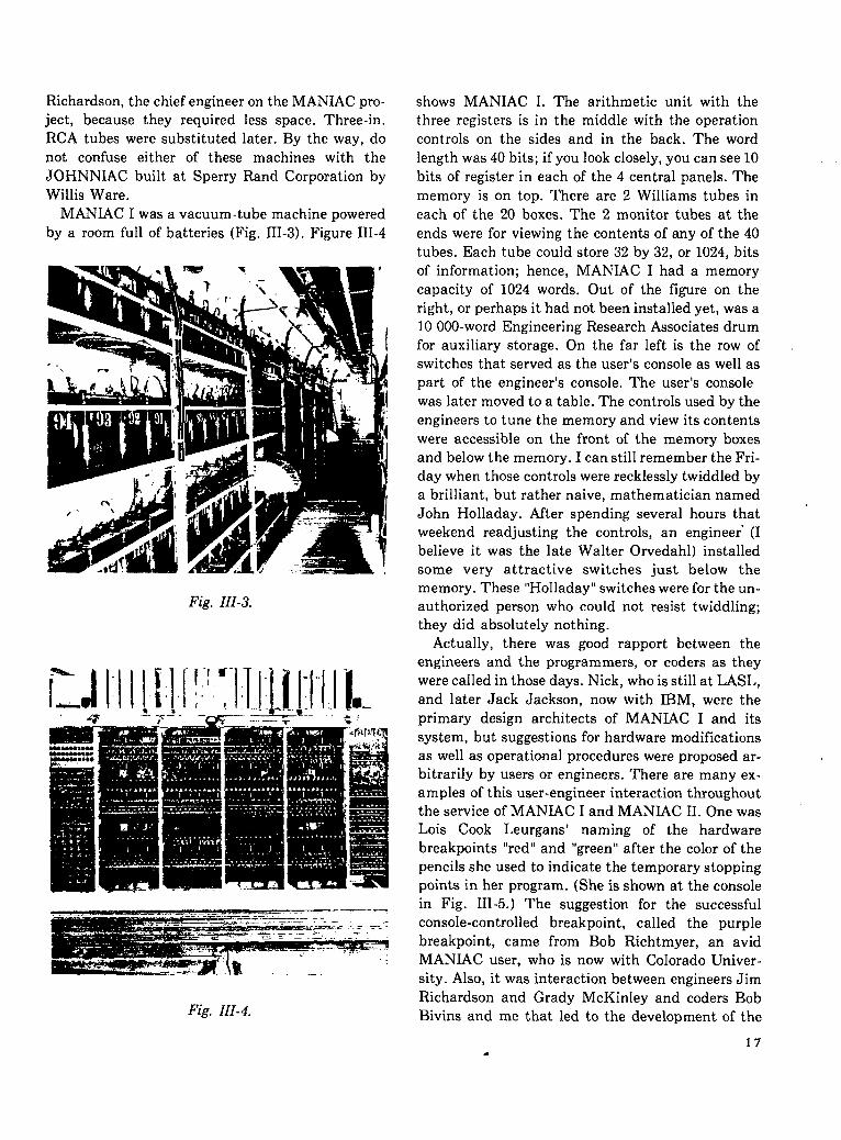
Richardson, the chief engineer on the MANIAC pro-ject, because they required less space, Three-in.RCA tubes were substituted later. By the way, donot confuse either of these machines with theJOHNNIAC built at Sperry Rand Corporation byWillis Ware.

MANIAC I was a vacuum-tube machine poweredby a room full of batteries (Fig. III-3). Figure III-4

Fig. III-3.

..-

~= -,—-—.—. =.’ ..-

Fig. III-4.

shows MANIAC I. The arithmetic unit with thethree registers is in the middle with the operationcontrols on the sides and in the back. The wordlength was 40 bits; if you look closely, you can see 10

bits of register in each of the 4 central panels. Thememory is on top. There are 2 Williams tubes ineach of the 20 boxes. The 2 monitor tubes at theends were for viewing the contents of any of the 40tubes. Each tube could store 32 by 32, or 1024, bitsof information; hence, MANIAC I had a memorycapacity of 1024 words. Out of the figure on theright, or perhaps it had not been installed yet, was a10 000-word Engineering Research Associates drumfor auxiliary storage. On the far left is the row ofswitches that served as the user’s console as well aspart of the engineer’s console. The user’s consolewas later moved to a table. The controls used by theengineers to tune the memory and view its contentswere accessible on the front of the memory boxesand below the memory. I can still remember the Fri-day when those controls were recklessly twiddled bya brilliant, but rather naive, mathematician namedJohn Holladay. After spending several hours that “weekend readjusting the controls, an engineer” (Ibelieve it was the late Walter Orvedahl) installedsome very attractive switches just below thememory. These “Holladay” switches were for the un-authorized person who could not resist twiddling;they did absolutely nothing.

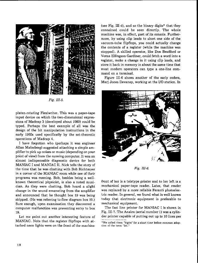
Actually, there was good rapport between theengineers and the programmers, or coders as theywere called in those days. Nick, who is still at LASL,and later Jack Jackson, now with IBM, were theprimary design architects of MANIAC I and itssystem, but suggestions for hardware modificationsas well as operational procedures were proposed ar-bitrarily by users or engineers. There are many ex-amples of this user-engineer interaction throughoutthe service of MANIAC I and MANIAC II. One wasLois Cook Leurgans’ naming of the hardwarebreakpoints “red” and “green” after the color of thepencils she used to indicate the temporary stoppingpoints in her program. (She is shown at the consolein Fig. III-5. ) The suggestion for the successfulconsole-controlled breakpoint, called the purplebreakpoint, came from Bob Richtmyer, an avidMANIAC user, who is now with Colorado Univer-sity. Also, it was interaction between engineers JimRichardson and Grady McKinley and coders BobBivins and me that led to the development of the

17.

platen-rotating Flexiwriter. This was a paper-tapeinput device on which the two-dimensional expres-sions of Madcap 3 (developed about 1960) could betyped. Perhaps the best example of all was thedesign of the bit manipulation instructions in theearly 1960s used specifically by the set-theoreticoperations of Madcap 4.

I have forgotten who (perhaps it was engineerAllan Malmberg) suggested attaching a simple am-plifier to pick up noises or music (depending on your

point of view) from the running computer. It was analmost indispensable diagnostic device for bothMANIAC I and MANIAC II. Nick tells the story ofthe time that he was chatting with Bob Richtmyerin a corner of the MANIAC room while one of theirprograms was running. Bob, besides being a well-known theoretical physicist, is also a noted musi-cian. As they were chatting, Bob heard a slightchange in the sound emanating from the amplifierand announced that he thought box 19 was beingskipped. (He was referring to flow diagram box 19.)Sure enough, upon examination they discovered acomputer malfunction was preventing entry to box19.

Let me point out another interesting feature ofMANIAC. Note that the register flipflops with at-

tached neon lights were on the front of the machine

(see Fig. III-4), and so the binary digits* that theycontained could be seen directly. The wholemachine was, in effect, part of its console. Further-more, by using clip leads to short one side of thevacuum-tube flipflops, you could actually changethe contents of a register (while the machine wasstopped). A skilled operator, like Don Bradford orVerna Ellingson Gardiner, could fetch a word into aregister, make a change in it using clip leads, andstore it back in memory in about the same time thatmost modern operators can type a one-line com-mand on a terminal.

Figure III-6 shows another of the early coders,Marj Jones Devaney, working at the I/O station. In

Fig. III-5.

Fig. III-6.

front of her is a teletype printer and to her left is amechanical paper-tape reader. Later, that readerwas replaced by a more reliable Feranti photoelec-

tric reader. In general, we found what is well knowntoday that electronic equipment is preferable tomechanical equipment.

The fast line printer for MANIAC I is shown inFig. III-7. The Analex (serial number 1) was a cylin-der printer capable of putting out up to 10 lines per—————___‘\Ve called t hem “bigits”for a shorttime beforecommonadop-tion of the term “bit.”

18

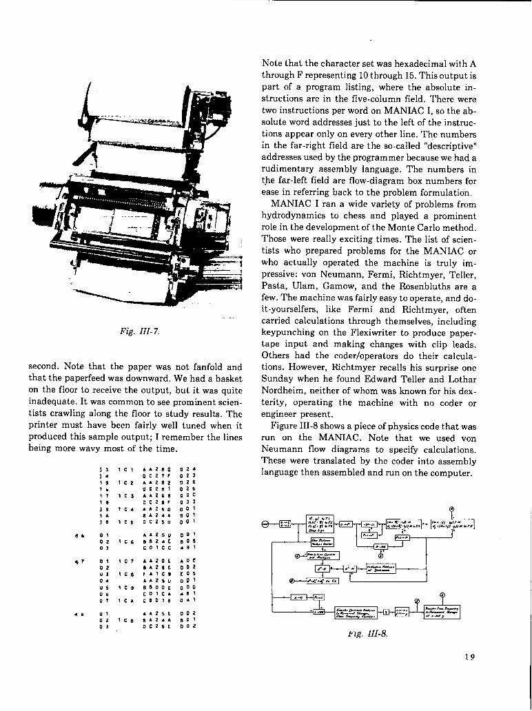
Fig. III- 7.

second. Note that the paper was not fanfold andthat the paperfeed was downward. We had a basketon the floor to receive the output, but it was quiteinadequate. It was common to see prominent scien-tists crawling along the floor to study results. Theprinter must have been fairly well tuned when itproduced this sample output; I remember the linesbeing more wavy most of the time.

46

+7

4U

J5 ICI A4213Q 024]4 Dcz?r 02s

15 !C2 &A28z 026!b 0C2B1 025

17 1C3 AA2C8 f)oc

1s ocz~r 033

J9 1C4 AA 250 ~’al

1A 0A 24A Bgl

JO 1C5 0C25U op\

01 AA25Q 00!

02 1C6 B1324f. 005

03 Colcc 491

01 lCT AA20t Aoc

02 OA25f 002

us Ice ?AICW CDS

04 AA2SU ~g!

us 1C9 .9800C 000

U6 cOt CA 481

07 lCA CS 018 041

U1 AA 25& 002

02 ICB fiA 24A sot

03 Ocz%f 002

Note that the character set was hexadecimal with Athrough F representing 10 through 15. This output ispart of a program listing, where the absolute in-structions are in the five-column field. There weretwo instructions per word on MANIAC I, so the ab-solute word addresses just to the left of the instruc-tions appear only on every other line. The numbersin the far-right field are the so-called “descriptive”addresses used by the programmer because we had arudimentary assembly language. The numbers inthe far-left field are flow-diagram box numbers forease in referring back to the problem formulation.

MANIAC I ran a wide variety of problems fromhydrodynamics to chess and played a prominentrole in the development of the Monte Carlo method.Those were really exciting times. The list of scien-tists who prepared problems for the MANIAC orwho actually operated the machine is truly im-pressive: von Neumann, Fermi, Richtmyer, Teller,Pasta, Ulam, Gamow, and the Rosenbluths are afew. The machine was fairly easy to operate, and do-it-yourselfers, like Fermi and Richtmyer, oftencarried calculations through themselves, includingkeypunching on the Flexiwriter to produce paper-tape input and making changes with clip leads.Others had the coder/operators do their calcula-tions. However, Rlchtmyer recalls his surprise oneSunday when he found Edward Teller and LotharNordheim, neither of whom was known for his dex-terity, operating the machine with no coder orengineer present.

Figure HI-8 shows a piece of physics code that wasrun on the MANIAC. Note that we used vonNeumann flow diagrams to speci~ calculations.These were translated by the coder into assemblylanguage then assembled and run on the computer.

k’lg. 111-8.

19 I

We believe that the first “performance measure-ment” was done on MANIAC I. Using an inter-pretive approach, Gene Herbst (now with IBM),Nick, and I were able to get a dynamic count of theinstructions used in various calculations. Table HI-I

TABLE III-I

ANALYSIS OF THE CODE FOR A PROBLEM IN

HYDRODYNAMICS

AAABAC~:

AFBABBBC;s

KCBccCDCECFDADBDcDDDEDFEAEBECEDEE

K

F:FD

E

Totals

Vccabdary StaticSymbol Count

7c.

11s1

P;p:f

Count

13.s0.60.00.00.00.08.0

;:0.00.00.32.94.2

;:0.00.08.00.213.64.2240.s0.010.29.0

k;1.63.23.60.00.02.40.2

‘(%W34W309060

27:2149

000

33:9364477700

249:

41:11s476312

322:2430

d;

llti1003

00

8!

28333

Percentageof Dynamic

Count,—

12.31.00.00.00.00.19.67.s0.00.00.00.01.13.3

$:0.00.08.80.214.64.02.60.00.011.38.50.1

H3.83.70.00.00.00.2

Time

314.927.80.00.00.03.6

247.0193.40.00.00.00.316.646.820.134.60.00.0

2S92.983.0149.71197.8106.80.80.0

209.6100.3

Sk:6.4&s.oS3,00.00.00.06.1

Yxi

PercentageO( Time

5.40.40.00.00.00.04.23.30.00.00.00.00.20.80.30.60.00.04s.11.44.320.81.80.00.03.6

:;0.90.11.s1.40.00.00.00.1

shows the results for a hydrodynamics calculation.The very high percentage of time (45.1%) used bythe multiply instruction (DA) was noted for input tothe design of MANIAC II.

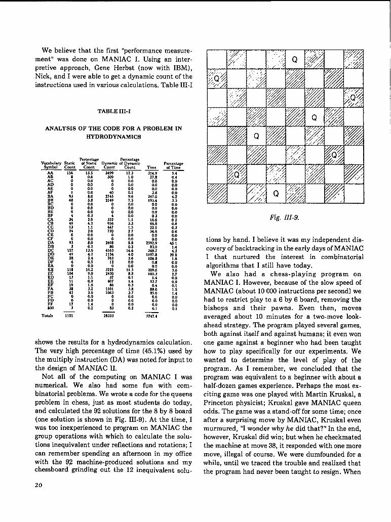
Not all of the computing on MANIAC I wasnumerical. We also had some fun with com-binatorial problems. We wrote a code for the queensproblem in chess, just as most students do today,and calculated the 92 solutions for the 8 by 8 board(one solution is shown in Fig. II-I-9). At the time, Iwas too inexperienced to program on MANIAC thegroup operations with which to calculate the solu-tions inequivalent under reflections and rotations; Ican remember spending an afternoon in my officewith the 92 machine-produced solutions and mychessboard grinding out the 12 inequivalent SOIU-

20

Fig. III-9.

tions by hand. I believe it was my independent dis-covery of backtracking in the early days of MANIACI that nurtured the interest in combinatorialalgorithms that I still have today.

We also had a chess-playing program onMANIAC I. However, because of the slow speed ofMANIAC (about 10000 instructions per second) wehad to restrict play to a 6 by 6 board, removing thebishops and their pawns. Even then, movesaveraged about 10 minutes for a two-move look-ahead strategy. The program played several games,both against itself and against humans; it even wonone game against a beginner who had been taughthow to play specifically for our experiments. Wewanted to determine the level of play of theprogram. As I remember, we concluded that theprogram was equivalent to a beginner with about ahalf-dozen games experience. Perhaps the most ex-citing game was one played with Martin Kruskal, aPrinceton physicist; Kruskal gave MANIAC queenodds. The game was a stand-off for some time; onceafter a surprising move by MANIAC, Kruskal evenmurmured, “I wonder why he did that?” In the end,however, Kruskal did win; but when he checkmatedthe machine at move 38, it responded with one moremove, illegal of course. We were dumbfounded for awhile, until we traced the trouble and realized thatthe program had never been taught to resign. When

I

confronted with no moves, it got stuck in a tightloop. As some of you may recall, tight loops were of-ten hard on electrostatic memories. In this case, thetight loop actually changed the program, creatingan exit from the loop, whereupon the program foundthe illegal move. You might call that a “learning”program.

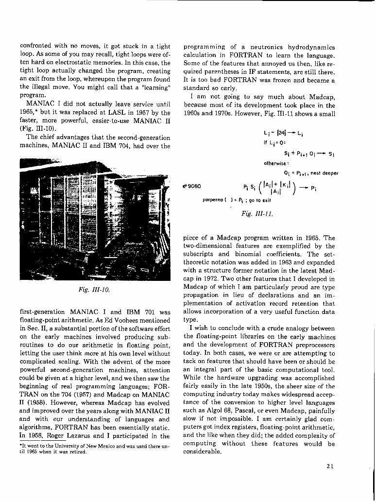
MANIAC I did not actually leave service until1965, * but it was replaced at LASL in 1957 by thefaster, more powerful, easier-to-use MANIAC II(Fig. III-10).

The chief advantages that the second-generationmachines, MANIAC II and IBM 704, had over the

Fig. III-10.

first-generation MANIAC I and IBM 701 wasfloating-point arithmetic. As Ed Voohees mentionedin “Sec. II, a substantial portion of the software efforton the early machines involved producing sub-routines to do our arithmetic in floating point,letting the user think more at his own level withoutcomplicated scaling. With the advent of the morepowerful second-generation machines, attentioncould be given at a higher level, and we then saw thebeginning of real programming languages; FOR-TRAN on the 704 (1957) and Madcap on MANIACII (1958). However, whereas Madcap has evolvedand improved over the years along with MANIAC IIand with our understanding of languages andalgorithms, FORTRAN has been essentially static.In 1958, Roger Lazarus and I participated in the——_*Itwentto theUniversityof NewMexicoandwasusedthereun-til 1965 whenit wasretired.

programming of a neutronics hydrodynamicscalculation in FORTRAN to learn the language.Some of the features that annoyed us then, like re-quired parentheses in IF statements, are still there.It is too bad FORTRAN was frozen and became astandard so early.

I am not going to say much about Madcap,because most of its development took place in the1960s and 1970s. However, Fig. III-II shows a small

Li - (24]~Li

if Li=O:

Si+Pi+l Qi~ Si

otherwise:

Qi = Pi+f , nest deeper

pi Si lAi~~i~Kil

( )

- pi

porperno ( ) = P, ; go to exil

Fig. III-1 1.

piece of a Madcap program written in 1965. Thetwo-dimensional features are exemplified by thesubscripts and binomial coefficients. The set-theoretic notation was added in 1963 and expandedwith a structure former notation in the latest Mad-cap in 1972. Two other features that I developed inMadcap of which I am particularly proud are typepropagation in lieu of declarations and an im-plementation of activation record retention thatallows incorporation of a very useful function datatype.

I wish to conclude with a crude analogy betweenthe floating-point libraries on the early machines

and the development of FORTRAN preprocessorstoday. In both cases, we were or are attempting totack on features that should have been or should bean integral part of the basic computational tool.While the hardware upgrading was accomplishedfairly easily in the late 1950s, the sheer size of thecomputing industry today makes widespread accep-tance of the conversion to higher level languagessuch as Algol 68, Pascal, or even Madcap, painfullyslow if not impossible. I am certainly glad com-puters got index registers, floating-point arithmetic,and the like when they did; the added complexity ofcomputing without these features would beconsiderable.

21

IvCONTRIBUTIONS TO MATHEMATICS

by

Roger B. Lazarus

First, I want to talk about a particular area ofphysics that I was involved in personally: the es-timating of the energy release of nuclear devices.Then, I will just mention, for the record and for thefun of reminiscence, some of the early problems thatI remember that were done in the early 1950s. Mostof them, but not all, were done on the MANL4C I.Finally I want to close with some speculativeremarks entitled, “Why Was It More Fun?”

The whole Los Alamos Project was started withthe “estimate” that if the fission reaction releasedboth energy and extra neutrons, then a chain reac-tion could be brought into existence that would givean explosion. And that is what it was all about.

In the 1940s during the war, and in the 1950s, themain challenging calculational problems were thoseof shock hydrodynamics and neutron transport.There was also radiation transport as a problem,and generally, that is easier than the neutrontransport.

The hydrodynamics problems are described byhyperbolic nonlinear partial differential equationsin space and time. It is the nature of those equationsthat discontinuities in the dependent variables can

come about spontaneously, so that thestraightforward replacing of partial differentialequations with partial difference equations can runinto trouble because the derivatives can become in-finite.

1 was not really quite sure of who did what first. Ifound in the preface of the 1957 edition ofRichtmyer’s book Difference Methods for Initial-

Value Problems, * the following sentence. “Finite-difference methods for solving partial differentialequations were discussed in 1928 in the celebratedpaper of Courant, Friedrichs, and Lewy but were

put to use in practical problems only about fifteen

———————.‘Kobert D. Rlchtmyer, .Di//ererzce Methods for Initial-ValuePrublcms, (IntersciencePublishers,Divisionof .John\$riley&Sons, 1957).

years later under the stimulus of wartimetechnology and with the aid of the first automaticcomputers ....” Well, the rest of the paragraph talksabout the LASL part of the whole thing.

The accounting machines that Jack Worltonshowed you, which were used primarily for shockhydrodynamics, were used only for the smooth partof the flow. The accounting machines would run asfar as they could, and when it was necessary to dothe shock fitting-to apply the jump conditionsacross the shock—that was done by hand. It wasthat hangup that led to the invention by Richtmyerand von Neumann of a thing called pseudo viscouspressure, which is an extra term added to the dif-ference equations that will smear out the shock overa few zones, the number of zones being essentiallyindependent of the shock speed and material. It willdo this in such a way as to preserve the importantquantities: shock strength and speed. That inven-tion was made specifically for a calculation done onthe SSEC. That was in the late 1940s. That methodof smearing is still in use.

There was a two-space dimensional R-Z cylin-drical geometry hydrodynamics code run on theENIAC, and I imagine it was the first two-

dimensional hydrodynamics done anywhere. Butusually, in the 1940s and the 1950s, one worked witha single space variable, either spherical symmetry orthe symmetry of an infinite cylinder. There are inhydrodynamic calculations both numerical in-stabilities and physical instabilities. Physical in-stabilities, such as mixing and picking up waveswhen one substance slides across another, are sup-pressed by the assumption of symmetry. This led to

a very deep part of the early computing problems.When I came to LASL in early 1951, my first

assignment was to do a yield calculation on a CPCfor a pure fission bomb. That machine was so simpleand so incapable, in modern terms, that at least onthe Model-1 CPC, it was not really possible to do

22

partial differential equations at all. Simplifyingassumptions were made, essentially parameterizingthe shape of everything, so that one could solve or-dinary differential equations. But that same year, inthe summer of 1951, my second job was to help witha code that had been written for SEAC for a thou-sand words of memory. It was really quite a substan-tial calculation that directly integrated the finitedifference approximations to the partial differentialequations. So there was quite a contrast, of which Ido not remember being particularly conscious. Thefocus was on the application—what approximationswere reasonable, what you needed to do, and thenyou looked around to see if you could do it.

The neutron transport part of things is describedby a linear integro-differential equation in which therate of change of the number of neutrons at a givenplace, direction, speed, and so on, depends on thescattering of all the neutrons at that point and goingin all directions. There was quite a range of dif-ficulty for that problem. The easiest case I can thinkof was to find a steady-state solution for a system ofspherical symmetry with a homogeneous scattererand within the diffusion limit, which is to say shortmean free path. That really is a very simpleproblem, The hardest, perhaps, would be somethingwhere there was no spatial symmetry, where thescatterers were in motion, where the mean free pathwas long compared to the dimensions, and, as an ex-tra difficulty, perhaps there were only a fewneutrons involved so that you had a discrete func-

tion.A problem geared to this latter class was most dif-

ficult and was what led to what is perhaps the most,or at least one of the most, far-reaching LASL in-ventions, namely, the Monte Carlo method. In fact,one of the most important early problems was thatof initiation probability—given a slightly super-critical assembly and one neutron, what is theprobability that that neutron, before being absorbedor escaping or having all its daughters escape, willlead to an explosive chain reaction? You candescribe Monte Carlo easily in that tranport con-text, which is where it is perhaps most obviously ap-plicable, but Monte Carlo grew in conjunction withthe growth of probability theory itself. Now it is ex-tremely widespread and used far from transportproblems where you are actually tracking things.

The first method that I used, on the CPC code forthe neutron transport problem, was called Serber-

Wilson. I assume it was invented in part by Serberand in part by Wilson. It had a lot of hyperbolicfunctions, and exponential integrals that were allentangled with the hyperbolic functions; and oneused those marvelous WPA (Work Project Ad-ministration) tables, which were perhaps the onlygood result of the Depression of the 1930s. The CPC,at least the Model-2 CPC, also had those functions.It had an electronic 604, or whatever it was, thatwould give you those. But the terms and expressionscontaining these functions were not physical expres-sions, and they were very difficult to scale. So whenI moved from the CPC to MANIAC I, carrying overSerber-Wilson, I found myself building essentiallyfloating-point software—automatic scalingsoftware. It was very annoying. Luckily, this wasreplaced by the family of methods Bengt Carlsoncame up with in the early 1950s and which are still,at least generically, the primary method of choicefor neutron transport. The dependent variables were

the currents themselves, the neutrons per squarecentimeter per second for certain energies, and theywere easy to scale. It was a tremendous blessing forfixed point. It also happened to be a fundamentallysuperior method in the long run.

From the CPC to the IBM STRETCH computer,there was approximately a factor of 104 increase inspeed and in memory size. The factor in run time fora typical yield calculation was 10”. Beginning on theCPC, at the end on STRETCH, and in fact today onCRAY-1, the really difficult problems take about 15hours and the easy ones take half an hour. Anotherthing that has not changed, besides the run time, isthe agreement between calculation and experiment,by an appropriate measure. At least, one can ob-serve that tests of nuclear devices still seem to benecessary. The answer to that paradox is, of course,the increase in complexity of the things we are try-ing to do. When we say 10% agreement, we do notmean between the same measures and quantities. Itmight be between some spectrum now, and it wasbetween some single number then.

I would like to wrap up this part on estimatingyields by particularly stressing the word estimating,

the difference that is suggested by the connotationof estimating uersus calculating. It seems to me thatwe were more conscious then that we were es-timating something. I remember quite early think-ing in terms of what I called the fudge function,which was simply a function over a parameter space

23

whose value is the ratio of the truth to what Icalculated. I saw my job, which was to predict theenergy release of some proposed design, as being aproblem in interpolation or extrapolation on thefudge function. I was calculating the yield for agiven design, but that is not the number I wouldpredict. I would interpolate or extrapolate on all theparameters I could think of and get the fudge func-tion value, 1.32 or whatever, and multiply theanswer by that. The trouble, of course, is the un-known dimensionality of the parameter space,which is to say knowing which of the probably in-finite number of things that were actually changedwere relevant. There were certainly times when onethought that the phase of the moon was the relevantparameter that would explain the mystery.

The physics that we added as time passed and ascomputers grew in capability was added, in general,where this fudge function was ill-behaved orperhaps where we only had a single point. To say wehad only a single point is equivalent to saying thatwe were starting into a new dimension, wheresomething was to be varied for the first time. Thenwe could clearly not interpolate, nor could we ex-trapolate. We could either assume it did not matter,which in some cases was patently absurd, or wewould have to add to the physics. But, all the timewe were conscious of the fact that we could not addall the physics. If we got a correct answer, it had toimply that the errors had cancelled precisely. Therewas no possibility that we would calculate all theprocesses correctly. The process of adding physicswas one usually of replacing what I always dis-tinguished as fudge ~actors (which are usually thingscalled the effective such and such, or the netequivalent so and so) with the relevant equation.For example, in the early days, we did not keep scat-tering cross sections as a function of energy. We keptthe one number that was the cross section averagedover the fission spectrum or whatever approximate

energy spectrum we expected.Then, with all these fudge factors, of which we

had really quite a few, there was a process of tuningthe code to give an attractive fudge function,ideally, one which would be unity over all themeasured points, but in any case, something thatyou felt comfortable with. That was part of the job:to tune the code. I remember that just before the 704came we had a 701 code that was really nicely tuned.

When we moved to the 704, we threw away all those

scale factors, all those powers of 2, with great joybecause they were really hard to keep track of. Ofcourse, the code on the 704 did not repeat, so westarted debugging. We went on and on until we werereally sure we had checked all the logic, and then wediscovered that one of our fudge factors that wethought was in there with a 2+2 scale factor was inthere with a 2-2. Given the pressure of time, the bestwe could do was change the fudge factor by 16 andswallow our pride. If we had put the correct fudgefactor into the 704 code, we would have loused upour fudge function. It stayed that way, as I remem-ber, until the test moratorium in the late 1950s.Then we finally had time to retwiddle.

Let me now switch to just giving a list and a fewcomments on some of the early MANIAC Iproblems. MANIAC I was a 1024-word machinewhen it was born—two instructions per word. Laterit got a drum. One of the first problems, besides theyield calculation that was my bread and butter, wassomething called Quintet, which was a five-dimensional integral for scattering corrections in ex-perimental physics. I remember it took approx-imately a second to get the integrand. It seemed likean easy problem until you really took some nominalnumber of points (I think a half a dozen when wefirst started) and took the fifth power; then sud-denly it was large. That is where I learned aboutGaussian quadrature. There were, of course, no in-dex registers then; a quintuple DO-loop involvedbringing out your instruction and adding the num-ber or subtracting the number from your addressand storing it back. Well, that was minor as aproblem.

A more important problem was the Fermi, Pasta,Ulam nonlinear oscillator investigation that led towhat is now still quite a live field, called solitontheory. There was the first Monte Carlo equation ofstate that was, I think invented by Marshall andArianna Rosenbluth (well, it is possible that Tellermade the original suggestion), where you tried tocalculate the actual equation of state of the materialby stochastic processes on sample molecules. Therewas what I assume was the first stellar evolutioncalculation, done by Art Carson and GeorgeGamow. There was, I think, the first chess; it wasnot strictly chess; it was 6 by 6 chess, It was aslightly reduced board. But it was quite important

24

as being, I think, the first or at. least a very earlyclass of computing that led to what is now called ar-tificial intelligence.

There was a code worked on by Verna Gardinerwith Gamow for trying to discover the code for DNAselection of amino acids, or whatever that is, whichof course was not successful. Other things were virialcoefficients, nuclear scattering problems, andSchrodinger equation integrations. Intranuclearcascades were another Monte Carlo thing; in a

heavy nucleus one actually tried to count theproduction of cascades of pions within the nucleus.

I noticed when the title was mentioned, it said

“mathematics.” I really have thought physics was

what LASL was about. But if I was really supposedto talk on math, I had better mention at least a cou-

ple of examples. There was a calculation of groupcharacters on MANIAC 1, done by Paul Stein andothers. There was perhaps the beginning of what a

lot of people now think of as experimentalmathematics, where you try things and explore us-ing the computer, trying to form conjectures or get

some new insight. It was believed, as I suppose it isby most mathematicians today, that ideas are not

worth anything until you prove something, but at

least there was an important role computers couldplay at the experimental level. One that I was in-volved with, an idea of Stan Ulam’s, was in the areaof pseudo prime numbers: integers that have not thedefining properties of prime numbers but have theirsame probability distribution within the set of allintegers. It was discovered that many of the proper-ties of primes apparently are due to their distribu-tion only, not to their unique defining property.There were also some cell multiplication studies;Ulam also was involved with that.

In parallel with all these problems (probablyevery one I mentioned was coded in absolute), therewas the business of subroutines and assemblyroutines. I do not really know who started what, orwhat credit LASL can take and get away with it, butit was just sort of common sense. You got tired ofcoding the sine function over and over again, so youborrowed somebody ’s. I remember personally beingquite negative about subroutines. It seemed to meoutrageous to lose control of where your numberswere in memory. That may be partly because of the1951 SEAC experience, which was the first thing Ihad todo with a really modern computer. I was han-

ded a code, all written, that required 1023 words. Iwas told we were going to take this in August andput it on the SEAC (which actually had a 1024-wordmemory) and “would you please make sure that it iscorrect. ” That seemed a reasonable thing at thetime. It was right there. Every bit was put down thatthe machine could see. So I worked for a couple ofmonths and I found three coding errors. As it turnedout, those were the only three coding errors therewere. Unfortunately, I made a mistake fixing thethree errors, so there was still a coding error when wegot to Washington. Again unfortunately, I neededtwo more words to fix those three errors, and that

came to 1025. Luckily that was a four-addressmachine—A, OP, B, C, and GO TO D—so youhad a free branch on every instruction. You couldput everything in where you wanted except forarrays, so I just picked a constant, decoded it, andarranged addresses so that some instruction had thenumerical value and off we went.

Maybe that story leads naturally into the topic,

“Why Was It More Fun?” I have six things listedhere, of which the first is “Maybe it was not morefun. ” There is selective recollection; there is thenostalgic fallacy. It is hard to judge. When the ses-sion started, it struck me as particularly appropriatethat they were doing that jackhammer work outsidebecause it was true that that was the feeling I got ofworking conditions around the computer, especiallyat New York University with UNIVAC I in 1953,with the air full of dust. But it was fun, and whatcould it have been? It could be that there were nooperating systems. There was more a feeling of managainst the elements; that you were searching forthe maximal exploitation of a set of hardware. It wasjust you and it. Perhaps it was that we had, I think,at least for these big problems, a deeper un-derstanding of a simpler calculation than we havetoday. Today I think we have a shallower un-derstanding of more complex calculations. Perhapsit was that there was no subdivision of labor. Atleast if you read some of the Marxists, they will tellyou most everything is less fun now because of sub-division of labor. People do not grasp the whole ofwhat they are doing. We certainly did then, becausewe did everything ourselves. Perhaps it was becausethere was no management or at least the manage-ment was invisible. In those days, at least accordingto my selective recollection, the scientist did

25

science, instead of management. Lastly, and with respect to the hardware and with respect to theperhaps more seriously, I will echo the point that I physics. We were so far from putting it all in. It wasthink Ed Voorhees made. There was more prior so new that we were not trapped into this confusionanalysis and estimating of what you were doing, es- between estimating and calculating. We did notpecially in the fixed-point computer era. There was think we were getting the answer to the originalmore checking; and there was more skepticism, both physics problem.

I

26 * U.S. GOVERNMENT PRINTING 0FFICE:1978–777-8S6 / S40