Representations for the Drazin inverses of 2 × 2 block matrices

Applied Mathematics and Computation 217 (2010) 2833–2842

Contents lists available at ScienceDirect

Applied Mathematics and Computation

journal homepage: www.elsevier .com/ locate/amc

Representations for the Drazin inverses of 2 � 2 block matrices q

Li Guo a,b, Xiankun Du a,*

a School of Mathematics, Jilin University, Changchun 130012, Chinab School of Mathematics, Beihua University, Jilin 132013, China

a r t i c l e i n f o

Keywords:Block matrixDrazin inverseIndex

0096-3003/$ - see front matter � 2010 Elsevier Incdoi:10.1016/j.amc.2010.08.019

q This work was supported by ‘‘211 Project” of Jil* Corresponding author.

E-mail addresses: [email protected] (L. Guo

a b s t r a c t

Let M denote a 2 � 2 block complex matrix A BC D

� �, where A and D are square matrices,

not necessarily with the same orders. In this paper explicit representations for the Drazininverse of M are presented under the condition that BDiC = 0 for i = 0,1, . . . ,n � 1, where n isthe order of D.

� 2010 Elsevier Inc. All rights reserved.

1. Introduction

For a square matrix A 2 Cn�n, the Drazin inverse of A is a matrix AD 2 Cn�n satisfying

AAD ¼ ADA; ADAAD ¼ AD; Akþ1AD ¼ Ak

for some nonnegative integer k. It is well-known that AD always exists and is unique. If Ak+1AD = Ak for some nonnegative inte-ger k, then so does for all nonnegative integer l P k, and the smallest nonnegative integer such that the equation holds isequal to ind(A), the index of A, which is defined to be the smallest nonnegative integer such that rank (Ak+1) = rank (Ak).We adopt the convention that A0 = In, the identity matrix of order n, even if A = 0, and the index of the zero matrix is definedto be 1. We write Ap = I � AAD. For more details we refer the reader to [1,4].

The Drazin inverse is first studied by Drazin [23] in associative rings and semigroups. The Drazin inverse of complexmatrices and its applications are very important in various applied mathematical fields like singular differential equations,singular difference equations, Markov chains, iterative methods and so on [4,5,24,31,35,37].

The study on representations for the Drazin inverse of block matrices essentially originated from finding the generalexpressions for the solutions to singular systems of differential equations [3–5], and then stimulated by a problem formu-

lated by Campbell [5]: establish an explicit representation for the Drazin inverse of 2 � 2 block matrices M ¼ A BC D

� �in

terms of the blocks of the partition, where the blocks A and D are assumed to be square matrices. For a deeper discussionof applications of the Drazin inverse of a 2 � 2 block matrix, we refer the reader to [4,37]. Until now, there has been no ex-plicit formula for the Drazin inverse of general 2 � 2 block matrices. Meyer and Rose [32], and independently Hartwig andShoaf [26], first gave the formulas for block triangular matrices, and since then many less restrictive assumptions are con-sidered [2,7,9,11–14,20,22,25,26,29,32–34,36], for example,

(1) BC = 0, BD = 0 and DC = 0 (see [20]);(2) BC = 0, DC = 0 (or BD = 0) and D is nilpotent (see [25]);

. All rights reserved.

in University.

), [email protected] (X. Du).

http://dx.doi.org/10.1016/j.amc.2010.08.019

mailto:[email protected]

mailto:[email protected]

http://dx.doi.org/10.1016/j.amc.2010.08.019

http://www.sciencedirect.com/science/journal/00963003

http://www.elsevier.com/locate/amc

2834 L. Guo, X. Du / Applied Mathematics and Computation 217 (2010) 2833–2842

(3) BC = 0 and DC = 0 (see [14]);(4) BC = 0, BDC = 0 and BD2 = 0 (see [22]);(5) BDpC = 0, BDDD = 0 and DDpC = 0 (see [22]).

Related topics are to find representations for the Drazin inverse and the generalized Drazin inverse of the sum of twomatrices [6,27,28,34] and operator matrices on Banach spaces [8,10,15–19,21].

It is clear that the condition in (4) above implies that BDiC = 0 for any nonnegative integer i, by which our work is moti-vated. Though this condition looks like a restrictive one, it is really weaker than many ones in the literature, especially thosein (1)–(5) and [16] which considers the generalized Drazin inverses, as shown in Examples 4.1 and 4.2, respectively.

In this paper, explicit expressions for the Drazin inverse of the 2 � 2 block matrix M are provided under the condition thatBDiC = 0 for i = 0,1, . . . ,n � 1, where n is the order of D, from which many results are unified and many formulas can be de-rived, especially those in [14,20,22,25].

For notational convenience, we define a sum to be 0, whenever its lower limit is bigger than its upper limit.

2. Preliminary

Lemma 2.1. For D 2 Cn�n and matrices B, C of appropriate orders, if BDiC = 0 for i = 0,1, . . . ,n � 1, then BDkC = 0 and B(DD)kC = 0for any nonnegative integer k.

Proof. Let f(k) = kn � a1kn�1�� an be the characteristic polynomial of D. By the Cayley–Hamilton theorem, f(D) = 0.

Thus

Dn ¼ a1Dn�1 þ � � � þ anI;

from which an induction on k yields BDkC = 0 for any nonnegative integer k. Since DD is expressible as a polynomial of D (see[1]), we have B(DD)kC = 0 for any nonnegative integer k. h

For simplicity of notation, we adopt the notation Ak(e) = (Ak + eI)�1 for any positive integer k, where e is a sufficiently smallpositive real number such that (Ak + eI)�1 exists.

Lemma 2.2 [30]. For A 2 Cn�n, the following statements are equivalent:(1) indðAÞ ¼ k;(2) k is the smallest nonnegative integer for which the limit lime?0ekA(e) exists.

Furthermore, for every nonnegative integer p, if p P ind (A) then

AD ¼ lime!0

Apþ1ðeÞAp:

Since all the limits in this paper are taken as e ? 0, we shall simply write ‘‘lim” instead of ‘‘lime?0”.

3. Main results

Let M denote a 2 � 2 block complex matrix A BC D

� �satisfying the following conditions:

A 2 Cm�m; D 2 Cn�n and BDiC ¼ 0; for i ¼ 0;1; . . . ;n� 1: ð3:1Þ

Then for any nonnegative integer k, a calculation yields

Mk ¼ Ak Bk

Ck Dk þ Nk

!; ð3:2Þ

where

Bkþ1 ¼ BkDþ AkB ¼ ABk þ BDk;

Ckþ1 ¼ CkAþ DkC ¼ DCk þ CAk;

Nkþ1 ¼ CkBþ NkD ¼ DNk þ CBk:

L. Guo, X. Du / Applied Mathematics and Computation 217 (2010) 2833–2842 2835

Then

Bk ¼Xk�1

i¼0

AiBDk�i�1;

Ck ¼Xk�1

i¼0

DiCAk�i�1; ð3:3Þ

Nk ¼X

iþlþj¼k�2

DiCAlBDj;

where i, j and l are all nonnegative integers. It is easy to verify that for any nonnegative integer i

BkDiCk ¼ 0; BkDiNk ¼ 0; NkDiCk ¼ 0; NkDiNk ¼ 0: ð3:4Þ

Lemma 3.1. Let M ¼ A BC D

� �, which satisfies the condition (3.1) . Then for any nonnegative integer k !

MkðeÞ ¼ AkðeÞ �AkðeÞBkDkðeÞ�DkðeÞCkAkðeÞ DkðeÞ � Dk

; ð3:5Þ

where Dk = Dk(e)(Nk � CkAk(e)Bk)Dk(e).

Proof. Denote by R the right-hand side of (3.5). Observe that BkDk(e)Ck = 0, BkDk(e)Nk = 0, DkCk = 0 and DkNk = 0 by Lemma 2.1and (3.4). Then a routine calculation yields R(Mk + e I) = I, whence Mk(e) = R. h

The following lemma is of independent interest.


� �, which satisfies the condition (3.1) . Then

indðAÞ 6 indðMÞ 6 indðAÞ þ 2indðDÞ:

Proof. By Lemma 3.1,

MðeÞ ¼AðeÞ �AðeÞBDðeÞ

�DðeÞCAðeÞ DðeÞ þ DðeÞCAðeÞBDðeÞ

� �:

For every nonnegative integer k,

ekMðeÞ ¼ ekAðeÞ �ekAðeÞBDðeÞ�ekDðeÞCAðeÞ ek DðeÞ þ DðeÞCAðeÞBDðeÞð Þ

!:

To prove the first inequality, take k = ind(M). Then by Lemma 2.2, limekM(e) exists, whence limekA(e) exists, and so ind(A) 6ind(M).

To prove the second inequality, let ind(A) = r, ind(D) = s and take k = r + 2s. Then from Lemma 2.2, the limits limekA(e) andlimekD(e) exist. Since

lim ekAðeÞBDðeÞ ¼ lim erAðeÞð ÞB e2sDðeÞ� �

;

lim ekDðeÞCAðeÞ ¼ lim e2sDðeÞ� �

C erAðeÞð Þ

and

lim ek DðeÞ þ DðeÞCAðeÞBDðeÞð Þ ¼ lim ekDðeÞ þ lim esDðeÞð ÞC erAðeÞð ÞB esDðeÞð Þ;

each exists, we see that limekM(e) exists. By Lemma 2.2, ind(M) 6 r + 2s. h

Remark 3.3. In Lemma 3.2 it is possible that ind(M) = ind(A) + 2 ind(D) or ind(M) < ind(D) as shown in Examples 4.3 and 4.4.


� �, which satisfies the condition (3.1) . Then MD has the following form !

MD ¼ AD b

c DD þ d;

where b, c and d are matrices such that


bc ¼ BDic ¼ bDiC ¼ 0; dc ¼ dDiC ¼ 0; bd ¼ BDid ¼ 0; d2 ¼ 0 ð3:6Þ

for any nonnegative integer i.


Mkþ1ðeÞ ¼ Akþ1ðeÞ �Akþ1ðeÞBkþ1Dkþ1ðeÞ�Dkþ1ðeÞCkþ1Akþ1ðeÞ Dkþ1ðeÞ � Dkþ1

!;

where Dk+1 = Dk+1(e)(Nk+1 � Ck+1Ak+1(e)Bk+1)Dk+1(e). We compute

Mkþ1ðeÞMk ¼ Akþ1ðeÞAk U

W Dkþ1ðeÞDk þK

!;

where

U ¼ Akþ1ðeÞBk � Akþ1ðeÞBkþ1Dkþ1ðeÞDk;

W ¼ �Dkþ1ðeÞCkþ1Akþ1ðeÞAk þ Dkþ1ðeÞCk;

K ¼ �Dkþ1ðeÞCkþ1Akþ1ðeÞBk þ Dkþ1ðeÞNk

� Dkþ1ðeÞðNkþ1 � Ckþ1Akþ1ðeÞBkþ1ÞDkþ1ðeÞDk:

Let ind(A) = r and ind(D) = s. Take k = r + 2s. Then k P ind(M) by Lemma 3.2. Hence, from Lemma 2.2,

MD ¼ limðMkþ1 þ eIÞ�1Mk ¼ limAkþ1ðeÞAk U

W Dkþ1ðeÞDk þK

!¼ AD lim U

lim W DD þ lim K

!:

Since MD exists and is unique, the limits limU, limW and limK exist, and let their values be b, c and d, respectively. Then

MD ¼ AD b

c DD þ d

!:

By Lemma 2.1 and the representations of U, W and K, we get (3.6). h

We are now in the position to prove our main results.

Theorem 3.5. Let M ¼ A BC D

� �, which satisfies the condition (3.1) , and let ind(A) = r, ind(D) = s and k P max{ind(M), ind(D)}.

ThenD

!
MD ¼ A X
Y DD þ Z;

where

X ¼Xs�1

i¼0

ðADÞiþ2BDiDp þ ApXr�1

i¼0

AiBðDDÞiþ2 � ADBDD;

Y ¼Xr�1

i¼0

ðDDÞiþ2CAiAp þ DpXs�1

i¼0

DiCðADÞiþ2 � DDCAD;

Z ¼ YAX þX

iþlþj¼k�2

ðDDÞkþ1�iCAlBDjDp þ DpDiCAlBðDDÞkþ1�j� �

�Xk�1

i¼0

ðDDÞiþ2CAiðAX þ BDDÞ þ ðYAþ DDCÞAiBðDDÞiþ2� �

:


MD ¼ AD b

c DD þ d

!;

where b, c and d satisfy the condition (3.6). Because MD exists and is unique, it is sufficient to prove b = X,c = Y and d = Z. Sincek P ind(M), the matrix MD is the unique one satisfying

MMD ¼ MDM;MDMMD ¼ MD;Mkþ1MD ¼ Mk:


Since Bc = bC = 0, Bd = 0 and dC = 0 by (3.6), we have

MMD ¼ AAD Abþ BDD

CAD þ Dc Cbþ DDD þ Dd

!;

MDM ¼ ADA ADBþ bD

cAþ DDC cBþ DDDþ dD

!:

Thus MMD = MDM is equivalent to

Abþ BDD ¼ ADBþ bD; ð3:7ÞCAD þ Dc ¼ cAþ DDC; ð3:8ÞCbþ Dd ¼ cBþ dD: ð3:9Þ

Since bc = 0, bd = 0, dc = 0 and d2 = 0 by (3.6), we have

ðMDÞ2 ¼ ðADÞ2 ADbþ bDD

cAD þ DDc cbþ ðDDÞ2 þ DDdþ dDD

!;

Since Bc = BDDc = 0, Bd = BDDd = 0 and d2 = 0 by (3.6), we have

MðMDÞ2 ¼ AD AADbþ AbDD þ BðDDÞ2

CðADÞ2 þ DcAD þ DDDc DD þ C

!;

where C = CADb + CbDD + Dcb + DDDd + DdDD. Thus MD = M(MD)2 is equivalent to

b ¼ AADbþ AbDD þ BðDDÞ2; ð3:10Þc ¼ CðADÞ2 þ DcAD þ DDDc; ð3:11Þd ¼ CADbþ CbDD þ Dcbþ DDDdþ DdDD: ð3:12Þ

Noting that Bkc = 0, Bkd = 0, Nkc = 0 and Nkd = 0, we see that

Mkþ1MD ¼ Akþ1AD Akþ1bþ Bkþ1DD

Ckþ1AD þ Dkþ1c Dkþ1DD þ Ckþ1bþ Nkþ1DD þ Dkþ1d

!:

By Lemma 3.2, k P ind(A) and by assumption, k P ind(D). Thus Mk+1MD = Mk is equivalent to

Bk ¼ Akþ1bþ Bkþ1DD; ð3:13ÞCk ¼ Ckþ1AD þ Dkþ1c; ð3:14ÞNk ¼ Ckþ1bþ Nkþ1DD þ Dkþ1d: ð3:15Þ

Similarly, noting that bCk = 0, bNk = 0, dCk = 0 and dNk = 0, we see that MDMk+1 = Mk is equivalent to

Bk ¼ ADBkþ1 þ bDkþ1; ð3:16ÞCk ¼ cAkþ1 þ DDCkþ1; ð3:17ÞNk ¼ cBkþ1 þ DDNkþ1 þ dDkþ1: ð3:18Þ

Since Bk+1 = BkD + AkB, the Eq. (3.13) gives Ak+1b = BkDp � AkBDD, whence

AADb ¼ ðADÞkþ1BkDp � ADBDD: ð3:19Þ

Since Bk+1 = ABk + BDk, the Eq. (3.16) gives bDk+1 = ApBk � ADBDk, whence

bDDD ¼ ApBkðDDÞkþ1 � ADBDD:

From (3.7) and the last equation, we deduce that

AbDD ¼ bDDD þ ADBDD � BðDDÞ2 ¼ ApBkðDDÞkþ1 � BðDDÞ2:

Substituting (3.19) and the last equation into (3.10), we have

b ¼ ðADÞkþ1BkDp þ ApBkðDDÞkþ1 � ADBDD:


It follows from (3.3) that

b ¼Xk�1

i¼0

ðADÞiþ2BDiDp þ ApXk�1

i¼0

AiBðDDÞiþ2 � ADBDD:

Since k P max{ind(M),ind(D)} P ind(A), we have

b ¼Xs�1

i¼0

ðADÞiþ2BDiDp þ ApXr�1

i¼0

AiBðDDÞiþ2 � ADBDD ¼ X:

Similarly, by (3.8), (3.11), (3.14), (3.17) and (3.3), we get

c ¼ ðDDÞkþ1CkAp þ DpCkðADÞkþ1 � DDCAD ¼Xr�1

i¼0


i¼0

DiCðADÞiþ2 � DDCAD ¼ Y :

Moreover, from (3.9), we obtain

DdDD ¼ dDDD þ ðcB� CbÞDD: ð3:20Þ

By (3.15),

DDDd ¼ ðDDÞkþ1ðNk � Ckþ1b� Nkþ1DDÞ:

Since Ck+1 = CkA + DkC and Nk+1 = CkB + NkD, it follows that

DDDd ¼ ðDDÞkþ1ðNk � CkAb� DkCb� NkDDD � CkBDDÞ ¼ ðDDÞkþ1NkDp � ðDDÞkþ1CkðAbþ BDDÞ � DDCb: ð3:21Þ

Similarly, from (3.18) and the fact that Bk+1 = ABk + BDk and Nk+1 = DNk + CBk, we obtain

dDDD ¼ ðNk � cBkþ1 � DDNkþ1ÞðDDÞkþ1 ¼ DpNkðDDÞkþ1 � ðcAþ DDCÞBkðDDÞkþ1 � cBDD: ð3:22Þ

Substituting (3.20) into (3.12), we have

d ¼ CADbþ CbDD þ Dcbþ DDDdþ dDDD þ ðcB� CbÞDD ¼ CADbþ Dcbþ cBDD þ DDDdþ dDDD:

By (3.21) and (3.22),

d ¼ CADbþ Dcb� DDCbþ ðDDÞkþ1NkDp þ DpNkðDDÞkþ1 � ðDDÞkþ1CkðAbþ BDDÞ � ðcAþ DDCÞBkðDDÞkþ1: ð3:23Þ

By (3.8),

CADbþ Dcb� DDCb ¼ cAb ¼ YAX:

Now substituting the last equation and (3.3) into (3.23), we get d = Z. h

Theorem 3.5 has the following dual version.

Theorem 3.6. Let M ¼ A BC D

� �with A 2 Cm�m and D 2 Cn�n, and let ind(A) = r, ind(D) = s and k P max{ind(M), ind(A)}. If

CAiB ¼ 0; for i ¼ 0;1; . . . ;m� 1;

then

MD ¼ AD þ Z0 X

Y DD

!;

where X and Y are as in Theorem 3.5 and

Z0 ¼ XDY þX

iþlþj¼k�2

ðADÞkþ1�iBDlCAjAp þ ApAiBDlCðADÞkþ1�j� �

�Xk�1

i¼0

ðADÞiþ2BDiðDY þ CADÞ þ ðXDþ ADBÞDiCðADÞiþ2� �

:

Proof. Let P ¼ 0 In

Im 0

� �. Then

M ¼ PD CB A

� �P�1:


Since CAiB = 0 for i = 0,1, . . . ,m � 1, Theorem 3.5 gives

D C

B A

� �D

¼ DD Y

X AD þ Z0

!;

where X and Y are as in Theorem 3.5 and Z0 is as in the statement of Theorem 3.6. Hence we have

MD ¼ PD C

B A

� �D

P�1 ¼ AD þ Z0 XY DD

!;

which completes the proof. h

From Theorem 3.5 we can easily deduce some results in [14,22] and of course some results in [20,25] by simplifying theexpressions of X, Y and Z.

Corollary 3.7 [14]. Let M ¼ A BC D

� �where A and D are square matrices with ind(A) = r and ind(D) = s. If BC = 0 and DC = 0,

then

MD ¼ AD X

CðADÞ2 DD þ CADX þ CXDD

!;

where X is as in Theorem 3.5.

Proof. It is sufficient to simplify Y and Z in Theorem 3.5 to the form given here under the assumption that BC = 0 and DC = 0.Clearly Y = C(AD)2. Taking k = r + 2s + 2, we have

Z ¼ CADX þ CXk�2

i¼0

AiBðDDÞiþ3 � CXk�1

i¼0

ADAiBðDDÞiþ2 ¼ CADX þ CApXk�2

i¼0

AiBðDDÞiþ3 � CADBðDDÞ2 ¼ CADX þ CXDD: �


� �where A and D are square matrices with ind(A) = r and ind(D) = s. If BC = 0, BDC = 0 and

BD2 = 0, then

MD ¼ AD ðADÞ3ðABþ BDÞY DD þ Z1

!;

where Y is as in Theorem 3.5 and

Z1 ¼ ðDDÞ3CBþXr�1

i¼0


i¼0

DiCðADÞiþ4 �X2

i¼0

ðDDÞiþ1CðADÞ3�i

!ðABþ BDÞ:

Proof. By Theorem 3.5 it is sufficient to prove that X = (AD)3(AB + BD) and Z = Z1. It is clear that

X ¼ ðADÞ2ðBDp þ ADBDDpÞ ¼ ðADÞ3ðABþ BDÞ:

It remains to prove Z = Z1. Taking k = r + 2s + 3, we have

Z ¼ YðADÞ2ðABþ BDÞ þXk�2

i¼0

ðDDÞiþ3CAiBþXk�3

i¼0

ðDDÞiþ4CAiBD�Xk�1

i¼0

ðDDÞiþ2CAiðADÞ2ðABþ BDÞ: ð3:24Þ

Furthermore,

YðADÞ2 ¼ DpXs�1

i¼0

DiCðADÞiþ4 � DDCðADÞ3;

Xk�2

i¼0

ðDDÞiþ3CAiBþXk�3

i¼0

ðDDÞiþ4CAiBD ¼ ðDDÞ3CBþXk�3

i¼0

ðDDÞiþ4CAiðABþ BDÞ: ð3:25Þ


Substituting (3.25) into (3.24), we have

Z ¼ ðDDÞ3CBþ DpXs�1

i¼0

DiCðADÞiþ4 þXk�3

i¼0

ðDDÞiþ4CAi �Xk�1

i¼0

ðDDÞiþ2CAiðADÞ2 � DDCðADÞ3 !

ðABþ BDÞ

¼ ðDDÞ3CBþ DpXs�1

i¼0

DiCðADÞiþ4 þXr�1

i¼0

ðDDÞiþ4CAiAp � DDCðADÞ3 � ðDDÞ2CðADÞ2 � ðDDÞ3CAD

!ðABþ BDÞ ¼ Z1: �


� �where A and D are square matrices with ind(A) = r and ind(D) = s. If BDpC = 0, BDDD = 0

and DDpC = 0, then

MD ¼AD Ps�1

i¼0ðADÞiþ2BDi

U0 DD þPs�1

i¼0Uiþ1BDi

0BBB@

1CCCA;

where for any nonnegative integer i,

Ui ¼Xr�1

j¼0

ðDDÞiþjþ2CAjAp þ DpCðADÞiþ2 �Xi

j¼0

ðDDÞjþ1CðADÞi�jþ1:

Proof. Since BDDD = 0, we have BDD = 0 and BDDDC = 0. Hence BDpC = 0 implies BC = 0, and DDpC = 0 implies DC = DDD2C.Thus BDiC = BDDDi+1C = 0 for any nonnegative integer i, that is, the condition in Theorem 3.5 is satisfied. Now it is clear thatX ¼

Ps�1i¼0 ðA

DÞiþ2BDi and Y = U0. We only need to prove that Z ¼Ps�1

i¼0 Uiþ1BDi. Take k = r + 2s + 2. Then by Theorem 3.5

Z ¼X

iþlþj¼k�2

ðDDÞkþ1�iCAlBDj þ Y �Xk�1

i¼0

ðDDÞiþ2CAi

!Xs�1

i¼0

ðADÞiþ1BDi

¼Xs�1

i¼0

Xk�2�i

j¼0

ðDDÞiþjþ3CAj

!BDi þ

Xs�1

i¼0

DpCðADÞiþ3 � DDCðADÞiþ2 �Xk�1

j¼0

ðDDÞjþ2CAjðADÞiþ1

!BDi:

Thus we only need to show that

Uiþ1 ¼Xk�2�i

j¼0

ðDDÞiþjþ3CAj þ DpCðADÞiþ3 � DDCðADÞiþ2 �Xk�1

j¼0

ðDDÞjþ2CAjðADÞiþ1:

Let us denote by W the right-hand side expression of the last equation. Then

W ¼Xr�1

j¼0

ðDDÞiþjþ3CAjAp þXk�2�i

j¼0

ðDDÞiþjþ3CAjþ1AD þ DpCðADÞiþ3 � DDCðADÞiþ2 �Xi

j¼0

ðDDÞjþ2CAjðADÞiþ1

�Xk�2�i

j¼0

ðDDÞiþjþ3CAjþ1AD ¼Xr�1

j¼0

ðDDÞiþjþ3CAjAp þ DpCðADÞiþ3 �Xiþ1

j¼0

ðDDÞjþ1CðADÞi�jþ2 ¼ Uiþ1: �

4. Examples

The following example gives a 2 � 2 block matrix M which does not satisfy the conditions given in (1)–(5) listed in Section1 but satisfies that in Theorem 3.5.

Example 4.1. Let M ¼ A BC D

� �, where A ¼ 1 �1

0 0

� �,

B ¼2 2 2�2 �2 �2

� �; C ¼

1 10 0�1 �1

0B@

1CA; D ¼

0 1 �10 1 00 �1 1

0B@

1CA:

Since DC – 0, BD2 – 0 and BDD – 0, the matrix M does not satisfy the conditions (1)–(5) given in Section 1. On the other hand,we can check that BDiC = 0 for i = 0,1,2,3. By Theorem 3.5, we obtain


MD ¼

1 �1 4 �6 40 0 0 �2 0�1 3 �12 11 �130 0 0 1 01 �3 12 �11 13

0BBBBBB@

1CCCCCCA:

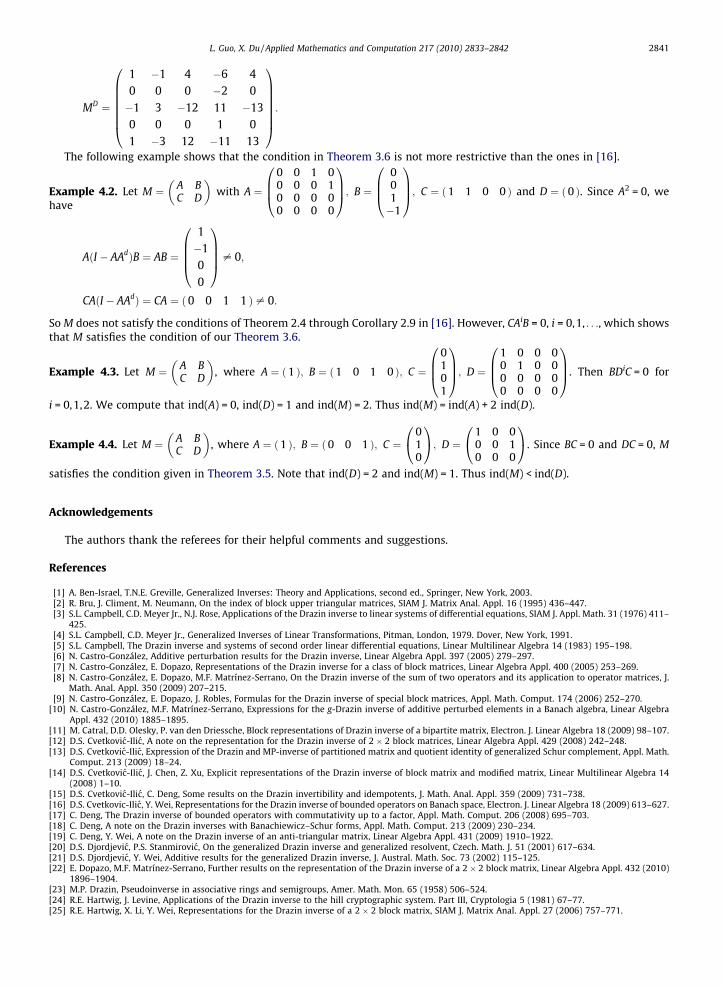
The following example shows that the condition in Theorem 3.6 is not more restrictive than the ones in [16].


� �with A ¼

0 0 1 00 0 0 10 0 0 00 0 0 0

0BB@

1CCA; B ¼

001�1

0BB@

1CCA; C ¼ 1 1 0 0ð Þ and D ¼ ð0 Þ. Since A2 = 0, we

have

AðI � AAdÞB ¼ AB ¼

1�100

0BBB@

1CCCA– 0;

CAðI � AAdÞ ¼ CA ¼ 0 0 1 1ð Þ – 0:

So M does not satisfy the conditions of Theorem 2.4 through Corollary 2.9 in [16]. However, CAiB = 0, i = 0,1, . . ., which showsthat M satisfies the condition of our Theorem 3.6.


� �, where A ¼ ð1 Þ; B ¼ ð1 0 1 0 Þ; C ¼

0101

0BB@

1CCA; D ¼

1 0 0 00 1 0 00 0 0 00 0 0 0

0BB@

1CCA. Then BDiC = 0 for

i = 0,1,2. We compute that ind(A) = 0, ind(D) = 1 and ind(M) = 2. Thus ind(M) = ind(A) + 2 ind(D).


� �, where A ¼ ð1 Þ; B ¼ ð0 0 1 Þ; C ¼

010

0@

1A; D ¼

1 0 00 0 10 0 0

0@

1A. Since BC = 0 and DC = 0, M

satisfies the condition given in Theorem 3.5. Note that ind(D) = 2 and ind(M) = 1. Thus ind(M) < ind(D).

Acknowledgements

The authors thank the referees for their helpful comments and suggestions.

References

[1] A. Ben-Israel, T.N.E. Greville, Generalized Inverses: Theory and Applications, second ed., Springer, New York, 2003.[2] R. Bru, J. Climent, M. Neumann, On the index of block upper triangular matrices, SIAM J. Matrix Anal. Appl. 16 (1995) 436–447.[3] S.L. Campbell, C.D. Meyer Jr., N.J. Rose, Applications of the Drazin inverse to linear systems of differential equations, SIAM J. Appl. Math. 31 (1976) 411–

425.[4] S.L. Campbell, C.D. Meyer Jr., Generalized Inverses of Linear Transformations, Pitman, London, 1979. Dover, New York, 1991.[5] S.L. Campbell, The Drazin inverse and systems of second order linear differential equations, Linear Multilinear Algebra 14 (1983) 195–198.[6] N. Castro-González, Additive perturbation results for the Drazin inverse, Linear Algebra Appl. 397 (2005) 279–297.[7] N. Castro-González, E. Dopazo, Representations of the Drazin inverse for a class of block matrices, Linear Algebra Appl. 400 (2005) 253–269.[8] N. Castro-González, E. Dopazo, M.F. Matrínez-Serrano, On the Drazin inverse of the sum of two operators and its application to operator matrices, J.

Math. Anal. Appl. 350 (2009) 207–215.[9] N. Castro-González, E. Dopazo, J. Robles, Formulas for the Drazin inverse of special block matrices, Appl. Math. Comput. 174 (2006) 252–270.

[10] N. Castro-González, M.F. Matrínez-Serrano, Expressions for the g-Drazin inverse of additive perturbed elements in a Banach algebra, Linear AlgebraAppl. 432 (2010) 1885–1895.

[11] M. Catral, D.D. Olesky, P. van den Driessche, Block representations of Drazin inverse of a bipartite matrix, Electron. J. Linear Algebra 18 (2009) 98–107.[12] D.S. Cvetkovic-Ilic, A note on the representation for the Drazin inverse of 2 � 2 block matrices, Linear Algebra Appl. 429 (2008) 242–248.[13] D.S. Cvetkovic-Ilic, Expression of the Drazin and MP-inverse of partitioned matrix and quotient identity of generalized Schur complement, Appl. Math.

Comput. 213 (2009) 18–24.[14] D.S. Cvetkovic-Ilic, J. Chen, Z. Xu, Explicit representations of the Drazin inverse of block matrix and modified matrix, Linear Multilinear Algebra 14

(2008) 1–10.[15] D.S. Cvetkovic-Ilic, C. Deng, Some results on the Drazin invertibility and idempotents, J. Math. Anal. Appl. 359 (2009) 731–738.[16] D.S. Cvetkovic-Ilic, Y. Wei, Representations for the Drazin inverse of bounded operators on Banach space, Electron. J. Linear Algebra 18 (2009) 613–627.[17] C. Deng, The Drazin inverse of bounded operators with commutativity up to a factor, Appl. Math. Comput. 206 (2008) 695–703.[18] C. Deng, A note on the Drazin inverses with Banachiewicz–Schur forms, Appl. Math. Comput. 213 (2009) 230–234.[19] C. Deng, Y. Wei, A note on the Drazin inverse of an anti-triangular matrix, Linear Algebra Appl. 431 (2009) 1910–1922.[20] D.S. Djordjevic, P.S. Stanmirovic, On the generalized Drazin inverse and generalized resolvent, Czech. Math. J. 51 (2001) 617–634.[21] D.S. Djordjevic, Y. Wei, Additive results for the generalized Drazin inverse, J. Austral. Math. Soc. 73 (2002) 115–125.[22] E. Dopazo, M.F. Matrínez-Serrano, Further results on the representation of the Drazin inverse of a 2 � 2 block matrix, Linear Algebra Appl. 432 (2010)

1896–1904.[23] M.P. Drazin, Pseudoinverse in associative rings and semigroups, Amer. Math. Mon. 65 (1958) 506–524.[24] R.E. Hartwig, J. Levine, Applications of the Drazin inverse to the hill cryptographic system. Part III, Cryptologia 5 (1981) 67–77.[25] R.E. Hartwig, X. Li, Y. Wei, Representations for the Drazin inverse of a 2 � 2 block matrix, SIAM J. Matrix Anal. Appl. 27 (2006) 757–771.


[26] R.E. Hartwig, J.M. Shoaf, Group inverses and Drazin inverses of bidiagonal and triangular Toeplitz matrices, J. Austral. Math. Soc. 24 (1977) 10–34.[27] R.E. Hartwig, G. Wang, Y. Wei, Some additive results on Drazin inverse, Linear Algebra Appl. 322 (2001) 207–217.[28] X. Li, Y. Wei, An expression of the Drazin inverse of a perturbed matrix, Appl. Math. Comput. 153 (2004) 187–198.[29] X. Li, Y. Wei, A note on the representations for the Drazin inverse of 2 � 2 block matrices, Linear Algebra Appl. 423 (2007) 332–338.[30] C.D. Meyer, Jr., Limits and the index of a square matrix, SIAM J. Appl. Math. 26 (1974) 469–478.[31] C.D. Meyer Jr., The condition number of a finite Markov chains and perturbation bounds for the limiting probabilities, SIMA J. Algebraic Discrete

Methods 1 (1980) 273–283.[32] C.D. Meyer Jr., N.J. Rose, The index and the Drazin inverse of block triangular matrices, SIAM J. Appl. Math. 33 (1977) 1–7.[33] M.F. Matrínez-Serrano, N. Castro-González, On the Drazin inverse of block matrices and generalized Schur complement, Appl. Math. Comput. 215

(2009) 2733–2740.[34] P. Patrício, R.E. Hartwig, Some additive results on Drazin inverses, Appl. Math. Comput. 215 (2009) 530–538.[35] B. Simeon, C. Fuhrer, P. Rentrop, The Drazin inverse in multibody system dynamics, Numer. Math. 64 (1993) 521–536.[36] Y. Wei, Expressions for the Drazin inverse of a 2 � 2 block matrix, Linear Algebra Appl. 45 (1998) 131–146.[37] N. Zhang, Y. Wei, Solving EP singular linear systems, Int. J. Comput. Math. 81 (2004) 1395–1405.

Documents

Representations for the Drazin inverses of 2 × 2 block matrices