Representation of Spatial Orientation by the Intrinsic ...sereno/170/readings/39-HeadDirModel.pdfThe Journal of Neuroscience, March 15, 1996, 16(6):2112-2126 Representation of Spatial

The Journal of Neuroscience, March 15, 1996, 16(6):2112-2126

Representation of Spatial Orientation by the Intrinsic Dynamics of the Head-Direction Cell Ensemble: A Theory

Kechen Zhang

Department of Cognitive Science, University of California at San Diego, La Jolla, California 92093-05 15

The head-direction (HD) cells found in the limbic system in freely moving rats represent the instantaneous head direction of the animal in the horizontal plane regardless of the location of the animal. The internal direction represented by these cells uses both self-motion information for inet-tially based updating and familiar visual landmarks for calibration. Here, a model of the dynamics of the HD cell ensemble is presented. The stability of a localized static activity profile in the network and a dynamic shift mechanism are explained naturally by synaptic weight distribution components with even and odd symmetry, respectively. Under symmetric weights or symmetric reciprocal connections, a stable activity profile close to the known directional tuning curves will emerge. By adding a slight asymmetry to the weights, the activity profile will shift continuously without

disturbances to its shape, and the shift speed can be controlled accurately by the strength of the odd-weight component. The generic formulation of the shift mechanism is determined uniquely within the current theoretical framework. The attractor dynamics of the system ensures modality-independence of the internal representation and facilitates the correction for cumulative error by the putative local-view detectors. The model offers a specific one-dimensional example of a computational mechanism in which a truly world-centered representation can be derived from observer-centered sensory inputs by integrating self-motion information.

Key words: head-direction cell; spatial orientation; attractor dynamics; dynamic shift mechanism; velocity integration; anterior thalamus; postsubiculum

1 BACKGROUND The head-direction (HD) cells found in the brains of freely moving rats have remarkable properties. They signal the instantaneous head direction of the animal in the horizontal plane regardless of the location of the animal in the environment (Ranck, 1985; Taube et al., 1990a). The system is striking in that its frame of reference is perfectly world-centered so that it can serve practically as a neural compass or gyroscope. The internal representation of head direction maintained by these cells is updated continually according to the head movement of the animal, even in total darkness (McNaughton et al., 1991; Mizu- mori and Williams, 1993). On the other hand, the system has a more “cognitive” aspect: It can use familiar landmarks to reset or calibrate the internal direction (Taube et al., 1990b; McNaughton et al., 1993; Goodridge and Taube, 1995; Taubc and Burton, 1995).

From a theoretical point of view, the HD system is very interesting. It provides compelling neurobiological evidence for stable attractor dynamics; at the same time, it forces consideration of the challenging problem of how to shift a stable activity profile (cf. Pouget and Scjnowski, 1995). The system is particularly appealing because it is intrinsically one-dimensional, and its operation is smooth and thus potentially subject to continuous analytical treat- ment. Finally, the properties of HD cells have clear parallels with

Received Sept. 7, IWS; rcviscd Dee. It;, 19%; acccptcd Dee. 20, 19%.

This research ww supported hy the McDonnell-Pew Center for Cognitive Ncuro- science at SW Diego and N;ttion:d Institutes of Health Grant MH47035 to M. I. Sercno. I cspcci;~lly thank M. 1. Scrcno and D. Zipscr for help snd support during the development of the model, .I. S. T;luhc for providing the data used in Figure 2, and

M. 1. Serene for wluablc comments xnd corrections on an carlicr version of the manuscript.

Corrcspondencc should hc addrcased to Kcchen Zhang, Dcpwtment of Cognitive

Science, University of Glifornia at San Diego, La Jolla, CA ‘)2(1X3-05 IS.

Copyright 0 19% Society for Ncurox%xx 0270-h474/Wl621 12.lS$OS.OO/O

the phenomena of human spatial perception, and they are beginning to provide a firm biological foundation for human experiences of spatial orientation (cf. Howard and Templeton, 1966; Gallistel, 1990).

Two major computational problems must be solved by the HD system. First, because the “sense of direction” reflects abstract qualities about spatial relationships, its neural representation must not depend on the modality of the sensory inputs. The biological system probably solves this problem by using sclf- sustaining activities in an attractor network. Second, as a truly world-centered representation, the “sense of direction” must be derived from primary sensory signals that arc all ccntcrcd to the body of the animal. This means that the overall reprcscntation is inherently dynamic and relies crucially on an updating mechanism that can compensate precisely for self-motion.

Several thcorctical models related to the HD cells have been proposed. Their dynamic shift mechanisms have various fcaturcs, including, in broad terms, the conjunction of the current head direction and movement information (McNaughton et al., 1991, 1995; Skaggs et al., 1995) the anticipatory activities in the thalamus (Blair, in press), and the rotation of sinusoidal arrays (Touretzky et al., 1993). Although the model here is consistent with the existing idea about the integration of both static and movement information, it stresses the central role of the intrinsic dynamics of the HD cell ensemble, in the same spirit as the model independently proposed by Skaggs et al. (1995). The present model has several new features. It has an explicit, analytical formulation of the dynamics of the HD cell continuum, and it unifies the descriptions of both the static behaviors and the dynamic shift mechanism in terms of the symmetry of the synaptic weight distribution. In the static case, the shape of the tuning curves is treated quantitatively as an emergent property of the network. In the dynamic case, the continuous shift mechanism,

the formulation of which can be determined uniquely, has accurate control over both the speed and the shape of traveling activity profile.

The theory has been reported in abstract form (Zhang, 1995).

2 BASIC PROPERTIES OF HD CELLS

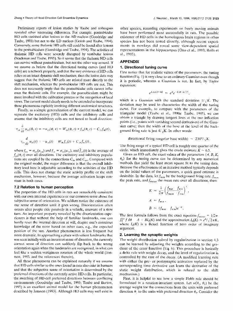
2.1 General descriptions HD cells were first found in the postsubiculum (also called dorsal presubiculum) in freely moving rats (Ranck, 1985). These cells have been studied systematically in several regions in rat brain, including the postsubiculum (Taube et al., 199Oa,b), the anterodorsal (AD) and lateral dorsal (LD) nuclei in the limbic thalamus (Mizumori and Williams, 1993; Blair and Sharp, 1995; Taube, 1995), and the posterior cingulate cortices (Chen et al., 1994a,b); in addition, there have been reports of a small number of HD cells in the striatum (Wiener, 1993; Mizumori and Cooper, 1995). See Figure 1 for a schematic summary.

Directional tuning A typical HD cell fires rapidly only when the head of the animal is pointing in a particular preferred direction in the horizontal plane, regardless of the location of the animal (Taube et al., 19YOa). As long as the animal is not disoriented, the preferred direction of an HD cell is the same everywhere, even if the animal is moved to different surroundings. The preferred directions of different cells seem to scatter uniformly. In contrast to the situation in many neocortical areas, HD cells with similar preferred directions do not cluster, and no obvious topographic neural organization has been found (Taube et al., 1YYOa; Taube, 1995; Sharp, in press).

Use of landmarks The preferred directions of HD cells arc based on the relative position of the animal with respect to the familiar stable landmarks. The rotation of a sole salient visual cue in a controlled environment would lead to an almost equal rotation of the prc- ferred directions of all HD cells (Taube et al., 1990b). A long- lasting association between the internal direction and a new environment can be established within minutes; when the internal direction is later in conflict with the familiar landmarks, the landmarks will dominate (Goodridge and Tdube, 1995; Taube and Burton, 1995).

Inertia& based updating Despite the strong control exerted by visual landmarks, the directional firings of HD cells persist in total darkness, presumably by integrating self-motion information (McNaughton et al., 1991; Mizumori and Williams, 1993). Understandably, the preferred

Zhang + Theory of Head-Direction Cell Ensemble Dynamics J. Neurosci., March 15. 1996, 16(6):2112-2126 2113

. anterodorsal nucleus

(AD): 60% La] . lateral dorsal nucleus

(LD): 60% Lb]

Figure I. A Papez-like circuit connects the major anatomical structures where HD cells have been found, with the highest percentages in the thalamus and the postsuh- iculum. References: [a] Tauhe (199.5), [b] Mizumori and Williams (1993), [c] cube et al. (1990a), [d] Tauhe (1993), [e] Sharp and Green (1994), [,f] Chen et al.

. subiculum: 0% le) (1994a). Many references to the anatomy can he found in Vogt and Gabriel (1993).

of the system

directions may drift during prolonged recordings (Mizumori and Williams, 1993).

Rigid frame

in darkness

The preferred directions of different HD cells are coupled tightly with one another so that the system can only bc rotated rigidly as a whole. That is, the rotation angles for the prcferrcd directions of different HD cells arc always the same, whether the rotation is caused by landmark rotation or disorientation of the animal (Taube et al., 1YYOb). The HD cells arc also rigidly coupled with the hippocampal place cells (Knierim et al., 1995).

Behavioral significance

The working hypothesis is that the internal direction represented by the HD cells corresponds to the internal “sense of direction” of the animal. The general manner in which the HD cells handle conflicting vestibular and the local-view information (Markus et al., 1990; McNaughton et al., 1993; Blair and Sharp, in press) is consistent with the behavioral results of spatial navigation (Mit- telstaedt and Mittelstaedt, 1980). After landmark rotation, both the choices of the animal in a behavioral task and the preferred directions of the HD cells rotated equally (Dudchenko and Taube, 1994). Finally, lesions to the postsubiculum (Taube et al., 1992) or inactivation of the LD nucleus (Mizumori et al., 1994) impaired the performances of the animal in spatial tasks.

Other properties of HD cells, including the anticipatory activities in the thalamus (section 5.3) and the effects of restraint and lesion stud& (section 7.l), will be discussed later.

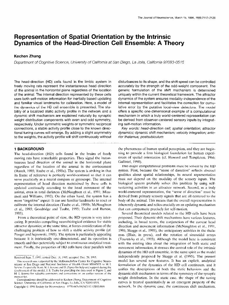
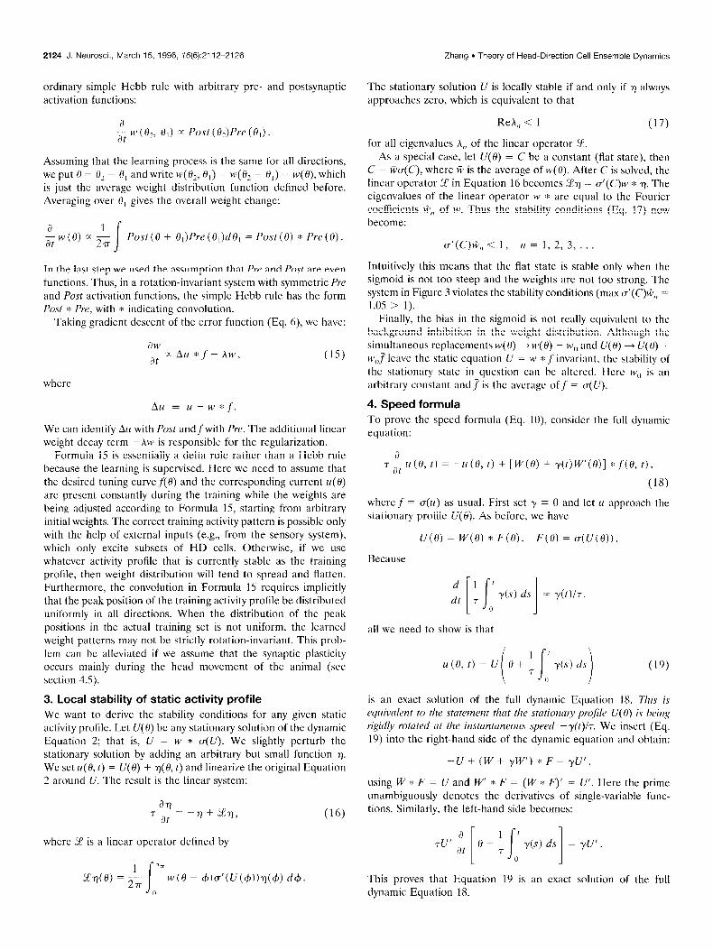
2.2 Directional tuning curve WC seek an analytical description for typical directional tuning cuwes of the HD cells in the postsubiculum and anterior thalamus, which have been studied extcnsivcly by Taubc and colleagues (Taube et al., 199Oa; Taube, 1995). A tuning curve plots the firing rate f as a function of the head direction 8, and it has a stereotyped triangular or Gaussian-like shape that can be fitted by the function:

f = A + Be~“O\~~~-fh) (1)

where 8,) is the preferred direction, and A, B, and K are all positive parameters (Fig. 2). Roughly speaking, K determines the sharp- ness of the tuning, whereas A and BeK are the background and the peak firing rates, respectively. The function (Eq. 1) is related to the so-called circular normal distribution (Johnson and Kotz, 1970). See Appendix 1 for more detailed discussion of the tuning curve.

At any given time, the most active HD cells are the ones with preferred directions close to the current head direction. The

2114 J. Neurosci., March 15, 1996, 76(6):2112-2126 Zhang l Theory of Head-Direction Cell Ensemble Dynamics

A Anterior Thalamus B Postsubiculum

-180’ -900 00 900 180’

80

60

0 -180’ -900 00 900 180’

Figure 2. A typical HD cell has stereotyped directional tuning curve. Its firing rate reaches maximum when the head direction fl is aligned with the preferred direction 0,). Data points and fitting curves are shown in both Cartesian and polar coordinates. A, An anterior thalamic HD cell with medium peak rate. Data from Figure 4B in Taubc (1995). Parameters: K = 8.08, A = 2.53 Hz, and BeK = 34.8 Hz. B, A postsubicular HD cell with high ueak rate. Data from Figure 3C in Taube ct al. (lY%aj. Parameters: K = 5.2’): A = 1.72 Hz, and BeK = 94.8 Hz. (Digital data courtesy of J. S. Tauhc.)

Head Direction 8 - 80 Head Direction 0 - 80

spread of activities among the whole population of HD cells as a function of the preferred direction (i.e., same head direction, different cells) is basically cquivalcnt to the directional tuning curve (i.e., same cell, diferent head directions). This is rigorously true only as a statistical statement. Let the head direction 0 be fixed. The average firing ratef(O,,) for the subpopulation of HD cells with the same preferred direction O,, is the weighted sum f(O,,) = C,p (a)fa( IO,, - 01) , where 01 = {A, B, K} is the set of parameters for characterizing the tuning curves,p(ol) is the probability density of (Y in the whole HD cell population, and the tuning function f&O, - 01) is the same asf in Equation 1.

3 BASIC DYNAMIC MODEL We consider a continuous formulation of the dynamics of the HD cell population. The model is concerned only with the average behaviors. For the time being, we do not distinguish HD cells in different anatomical regions. The average firing rate of all the HD cells with the same preferred direction 0 is described by a single scalar function f = f(0, t), which is also a function of time t. Similarly, u = ~(0, t) is the average net inputs or “synaptic currents” received by these units. They are assumed to be related by a sigmoid function:

f = CT(u).

The model is essentially one-dimensional with ring topology, and the distribution of the preferred directions is treated as continuous and uniform. It is important to note that the ring here is defined by the preferred directions, which are ultimately determined by the connections between the cells instead of by their physical positions in the brain; in fact, there are good theoretical reasons why proximity of physical positions does not imply the similarity of preferred directions (section 4.5).

The time evolution of the system has “standard” simplified continuous dynamics (Amari, 1972; Sejnowski, 1977; Hopfield, 1984) governed by the equation:

a11

T -it =-u+w*f, (2)

where the convolution is dcfincd by:

w(0, t) * f(0, t) = :, I

277 WC0 - $3 r)f(4, t) d$.

0

The convolution is involved because the system is assumed to be rotation-invariant; that is, the average synaptic weight w between two units with the preferred directions 0, and O2 should depend only on the difference 0, - Oz. We use the synaptic weight distribution function ~(0, t) to describe the average strength of the synaptic weights between two units with preferred directions dif- fering by the angle 0, with 0 > 0 indicating projections to counterclockwise neighbors and 0 < 0, to clockwise neighbors.

Parameter 7 is a time constant. We chose T = 10 msec in all simulations presented here. The behaviors of the system are not affected by the exact value of T, because the sole effect of changing T is equivalent to a change of the time scale.

It must be emphasized that in this system the reciprocal connections between two units arc not always equal. This implies that the projections from a given unit to its clockwise and counterclockwise neighbors can be different, or equivalently, the system in general is not reflection-invariant. In terms of the synaptic weight distribution function ~(0, t), this means that:

w(-0, t) # w(0, t).

The system is different from a Hopfield network, in which the existence of point attractors is guaranteed by the symmetry of the reciprocal connections (Cohen and Grossberg, 1983; Hopfield, 1984). In general, an arbitrary ~(0, t) can always be decomposed uniquely into even (“symmetric”) and odd (“antisymmetric”) components:

WC& t) = W,“,“(O> f) + w,,,,(O, t), (3)

with w,,,,(- 0, 4 = w,,,,(@ t> and wodd(- 0, 4 = -w,,dO, 4. The decomposition has a special meaning here. We assume that

W even is constant, whereas w Odd is modified rapidly during a head turn. When w,,‘,~, = 0, all the weights in the network are symmetric, and the system always settles into some static attractor state. This case corresponds to the self-sustaining HD cell firings in the absence

Zhang . Theory of Head-DIrectIon Cell Ensemble Dynamics J. Neurosci., March 15, 1996, 16(6):2112-2126 2115

Population of 360’ y Population of HD Cells HD Cells

of movements. When PV,,~~ # 0, a continuous shift of the activity spot will occur, which corresponds to the case of head turn. In this model, the ultimate effect of motion signals such as the vestibular input is to induce a small nonzcro odd component of the weight distribution. In a realistic neural circuit, the asymmetry could be implemented in a number of different ways (section 5.2).

Finally, we emphasize the close relationship between the continuous model and the more familiar form of neural n&work models with discrete units. Numerical simulation shows that as long as there are more than -50 units, the smooth behaviors of the corresponding discrete model are virtually independent of the exact number of units; that is, the continuous model starts to provide an adequate description of the dynamics. Therefore, in the following sections we do not explicitly consider the size of the network, except in section 4.5 on the effects of noisy weights, where the actual network size becomes relevant.

4 STATIONARY SELF-SUSTAINING ACTIVITIES

4.1 Origin of directional tuning We consider the behavior of the model system in the absence of any external input. In this case, the synaptic weight distribution is symmetric (i.e., reciprocal connections are equal) with local excitation and longer-range inhibition.

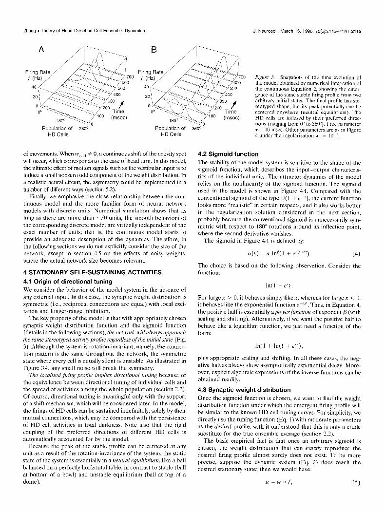
The key property of the model is that with appropriately chosen synaptic weight distribution function and the sigmoid function (details in the following sections), the network will always approach the same stereotyped activity profile regardless of the initial state (Fig. 3). Although the system is rotation-invariant, namely, the connection pattern is the same throughout the network, the symmetric state where every cell is equally silent is unstable. As illustrated in Figure 3A, any small noise will break the symmetry.

The localized firing profile implies directional tuning because of the equivalence between directional tuning of individual cells and the spread of activities among the whole population (section 2.2). Of course, directional tuning is meaningful only with the support of a shift mechanism, which will be considered later. In the model, the firings of HD cells can be sustained indefinitely, solely by their mutual connections, which may be compared with the persistence of HD cell activities in total darkness. Note also that the rigid coupling of the preferred directions of different HD cells is automatically accounted for by the model.

Because the peak of the stable profile can be centered at any unit as a result of the rotation-invariance of the system, the static state of the system is essentially in a neutral equilibrium, like a ball balanced on a perfectly horizontal table, in contrast to stable (ball at bottom of a bowl) and unstable equilibrium (ball at top of a dome).

Figure 3. Snapshots of the time evolution of the model obtained by numerical integration of the continuous Equation 2, showing the emergence of the same stable firing profile from two arbitrary initial states. The final profile has stereotyped shape, but its peak potentially can be centered anywhere (neutral equilibrium). The HD cells are indexed by their preferred direc-

360’ tions (ranging from 0” to 360”). Free parameter Q- = 10 msec. Other parameters arc as in Figure 4 under the regularization A,, = 10 ‘.

4.2 Sigmoid function

The stability of the model system is sensitive to the shape of the sigmoid function, which describes the input-output characteristics of the individual units. The attractor dynamics of the model relies on the nonlinearity of the sigmoid function. The sigmoid used in the model is shown in Figure 4A. Compared with the conventional sigmoid of the type I/( I + e ‘). the current function looks more “realistic” in certain respects, and it also works better in the rcgularization solution considered in the next section, probably because the conventional sigmoid is unnecessarily symmetric with respect to 180” rotations around its infection point, where the second derivative vanishes.

The sigmoid in Figure 4A is defined by:

(T(X) = a lnP( 1 + e’J@+c)). (4)

The choice is based on the following observation. Consider the function:

ln( 1 + er) .

For large x > 0, it behaves simply like X, whereas for large x < 0, it behaves like the exponential function e-l”‘. Thus, in Equation 4, the positive half is essentially apowerfunction of exponent /3 (with scaling and shifting). Alternatively, if we want the positive half to behave like a logarithm function, we just need a function of the form:

In(l + ln(1 + e’)),

plus appropriate scaling and shifting. In all these cases, the negative halves always show asymptotically exponential decay. More- over, explicit algebraic expressions of the inverse functions can be obtained readily.

4.3 Synaptic weight distribution Once the sigmoid function is chosen, we want to find the weight distribution function under which the emergent firing profile will be similar to the known HD cell tuning curves. For simplicity, we directly use the tuning function (Eq. 1) with moderate parameters as the desired profile, with it understood that this is only a crude substitute for the true ensemble average (section 2.2).

The basic empirical fact is that once an arbitrary sigmoid is chosen, the weight distribution that can exactly reproduce the desired firing profile almost surely does not exist. To be more precise, suppose the dynamic system (Eq. 2) does reach the desired stationary state; then we would have:

u=w*f, (5)

2116 J. Neurosci., March 15, 1996, 16(6):2112-2126 Zhang . Theory of Head-Direction Cell Ensemble Dynamics

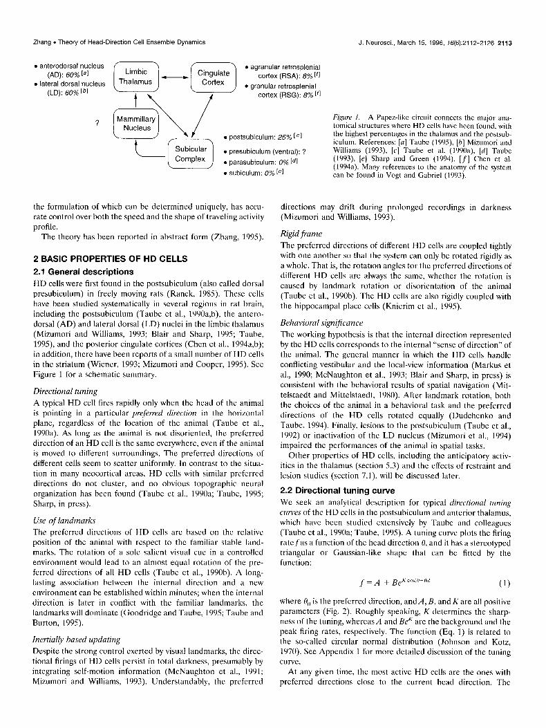
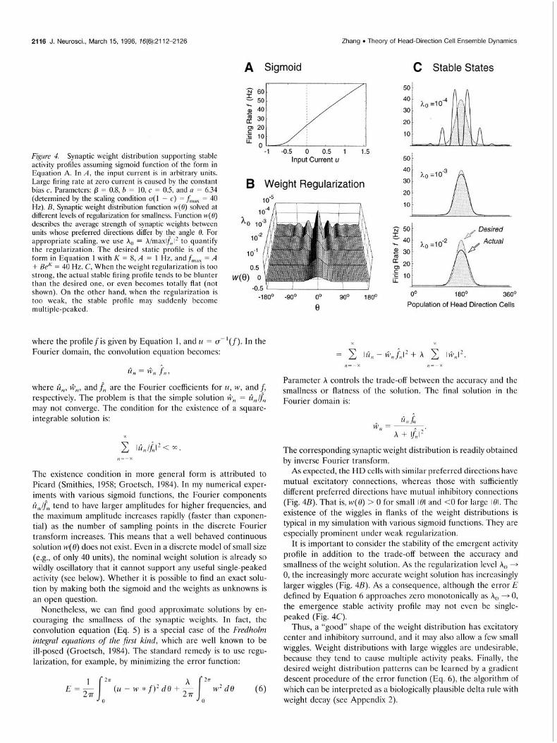
Figure 4. Synaptic weight distribution supporting stable activity profiles assuming sigmoid function of the form in Equation A. In A, the input current is in arbitrary units. Large firing rate at zero current is caused by the constant bias c. Paramctcrs: p = O.&O = 10, c = 0.5, and a = 6.34 (determined by the scaling condition ~(1 - c) = f,,,, = 40 Hz). B, Synaptic weight distribution function w(0) solved at different levels of regularization for smallness. Function IV(~) describes the average strength of synaptic weights between units whose preferred directions differ by the angle 0. For appropriate scaling, we use h, = h/maxlQ,,l’ to quantify the regularization. The desired static profile is of the form in Equation 1 with K = 8, A = 1 Hz, andf,,,, = A + BeK = 40 Hz. C, When the weight regularization is too strong, the actual stable firing profile tends to be blunter than the desired one, or even becomes totally flat (not shown). On the other hand, when the regularization is too weak, the stable profile may suddenly become multiple-peaked.

A Sigmoid

-1 -0.5 0 0.5 1 1.5 input Current u

B Weight Regularization 1O‘5

1o-4 I ’

-1800 -900 00 900 180’

0

where the profilefis given by Equation 1, and II = a-‘(f). In the Fourier domain, the convolution equation becomes:

11 !I ̂ = I$,, j,,>

where ir,,, )$,1, and i, are the Fourier coefficients for II, IV, and f, respectively. The problem is that the simple solution +,? = ti,,/‘, may not converge. The condition for the existence of a square- integrable solution is:

The existence condition in more general form is attributed to Picard (Smithies, 1958; Groetsch, 1984). In my numerical experiments with various sigmoid functions, the Fourier components ti,/f” tend to have larger amplitudes for higher frequencies, and the maximum amplitude increases rapidly (faster than exponential) as the number of sampling points in the discrete Fourier transform increases. This means that a well behaved continuous solution w(0) does not exist. Even in a discrete model of small size (e.g., of only 40 units), the nominal weight solution is already so wildly oscillatory that it cannot support any useful single-peaked activity (see below). Whether it is possible to find an exact solution by making both the sigmoid and the weights as unknowns is an open question.

Nonetheless, we can find good approximate solutions by en- couraging the smallness of the synaptic weights. In fact, the convolution equation (Eq. 5) is a special case of the Fredholm integral equations of the first kind, which are well known to be ill-posed (Groetsch, 1984). The standard remedy is to use regularization, for example, by minimizing the error function:

277 (u - w *f):do+& ‘k2de

I (6)

0

C Stable States

00 1800 360’

Population of Head Direction Cells

,,=-’ , , = - ,

Parameter A controls the trade-off between the accuracy and the smallness or flatness of the solution. The final solution in the Fourier domain is:

The corresponding synaptic weight distribution is readily obtained by inverse Fourier transform.

As expected, the HD cells with similar preferred directions have mutual -excitatory connections, whereas those with sufficientlv different preferred directions have mutual inhibitory connections (Fig. 4B). That is, w(0) > 0 for small 101 and <O for large 101. The existence of the wiggles in flanks of the weight distributions is typical in my simulation with various sigmoid functions. They are especially prominent under weak regularization.

It is important to consider the stability of the emergent activity profile in addition to the trade-off between the accuracy and smallness of the weight solution. As the regularization level h, + 0, the increasingly more accurate weight solution has increasinglv larger wiggles (Fig. 4B). As a consequence, although the error”E defined by Equation 6 approaches zero monotonically as h, + 0, the emergence stable activity profile may not even be single- peaked (Fig. 4C).

Thus, a “good” shape of the weight distribution has excitatory center and inhibitory surround, and it may also allow a few small wiggles. Weight distributions with large wiggles are undesirable, because they tend to cause multiple activity peaks. Finally, the desired weight distribution patterns can be learned by a gradient descent procedure of the error function (Eq. 6), the algorithm of which can be interpreted as a biologically plausible delta rule with weight decay (see Appendix 2).

Zhang . Theory of Head-Direction Cell Ensemble Dynamics

A Effects of Noisy Weights B Drift Speed

‘;;‘ N= 32.~ = 0.06 g 40

$J 30 2 20 Initial F 10 States .- it

0 00 iSO’= 3600

$4 40

al 30 Final 2 20 States 0 ‘0 .F 0

Time (set)

C Scaling

&=o.l

b:l::l-!!:.

& = 0.01

30 50 100 200 300

Network Size N

E 00 1800 360’


4.4 Stability of self-sustaining activities As shown in Appendix 3, the local stability of an arbitrary stationary activity profile can be determined by examining the linearized dynamic equation. As a special case, we can show that the symmetry breaking in Figure 3A is inevitable, because the stability conditions for the flat state are violated. If the parameter c (bias in the sigmoid function) is sufficiently reduced (e.g., setting c = 0 in the same example), however, both the single-peaked state and the

flat state can become locally stable. The stability of the flat state might be controlled actively in

the biological system. For example, by simply increasing the overall inhibition level and stabilizing the low-activity flat state, the whole system can effectively be shut down, which might be useful for preventing undesirable Hebbian learning induced by prolonged activation of a fixed group of HD cells, for example, during sleep.

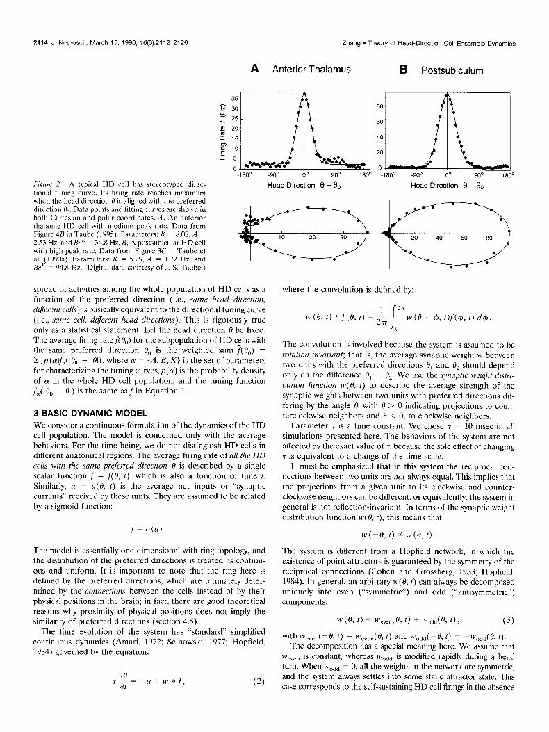
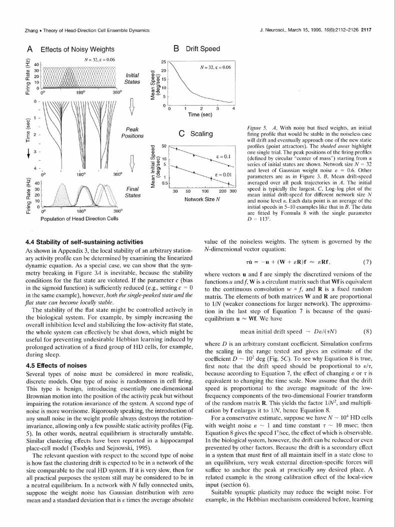
4.5 Effects of noises Several types of noise must be considered in more realistic, discrete models. One type of noise is randomness in cell firing. This type is benign, introducing essentially one-dimensional Brownian motion into the position of the activity peak but without impairing the rotation-invariance of the system. A second type of noise is more worrisome. Rigorously speaking, the introduction of any small noise in the weight profile always destroys the rotation- invariance, allowing only a few possible static activity profiles (Fig. 5). In other words, neutral equilibrium is structurally unstable. Similar clustering effects have been reported in a hippocampal place-cell model (Tsodyks and Sejnowski, 1995).

The relevant question with respect to the second type of noise is how fast the clustering drift is expected to be in a network of the size comparable to the real HD system. If it is very slow, then for all practical purposes the system still may be considered to be in a neutral equilibrium. In a network with N fully connected units, suppose the weight noise has Gaussian distribution with zero mean and a standard deviation that is E times the average absolute

J. Neurosci., March 15, 1996, 16(6):2112-2126 2117

F@re 5. A, With noisy but fised weights, an initial firing profile that would be stable in the noiseless case will drift and eventually approach one of the new static profiles (point attractors). The shaded areas highlight one single trial. The peak positions of the firing profiles (defined by circular “center of mass”) starting from a series of initial states are shown. Nehvork size N = 32 and level of Gaussian weight noise E = 0.6. Other parameters are as in Figure 3. B, Mean drift-speed averaged over all peak trajectories in A. The initial speed is typically the largest. C, Log-log plot of the mean initial drift-speed for different network size N and noise level E. Each data point is an average of the initial speeds in 5-10 examples like that in B. The data are fitted by Formula 8 with the single parameter D = 113”.

value of the noiseless weights. The sytsem is governed by the N-dimensional vector equation:

ni = -u + (W + &R)f = &Rf, (7)

where vectors u and f are simply the discretized versions of the functions II and f, W is a circulant matrix such that Wf is equivalent to the continuous convolution tv * f, and R is a fixed random matrix. The elements of both matrices W and R are proportional to l/N (weaker connections for larger network). The approximation in the last step of Equation 7 is because of the quasi- equilibrium II - Wf. We have

mean initial drift speed - DE/(TN) (8)

where D is an arbitrary constant coefficient. Simulation confirms the scaling in the range tested and gives an estimate of the coefficient D - 10’ deg (Fig. SC). To see why Equation 8 is true, first note that the drift speed should be proportional to ~/r,

because according to Equation 7, the effect of changing E or T is equivalent to changing the time scale. Now assume that the drift speed is proportional to the average magnitude of the low- frequency components of the two-dimensional Fourier transform of the random matrix R. This yields the factor 1/N2, and multipli- cation by f enlarges it to l/N, hence Equation 8.

For a conservative estimate, suppose we have N - 10” HD cells with weight noise E - 1 and time constant 7 - 10 msec; then Equation 8 gives the speed l”/sec, the effect of which is observable. In the biological system, however, the drift can be reduced or even prevented by other factors. Because the drift is a secondary effect in a system that must first of all maintain itself in a state close to an equilibrium, very weak external direction-specific forces will suffice to anchor the peak at practically any desired place. A related example is the strong calibration effect of the local-view input (section 6).

Suitable synaptic plasticity may reduce the weight noise. For example, in the Hebbian mechanisms considered before, learning


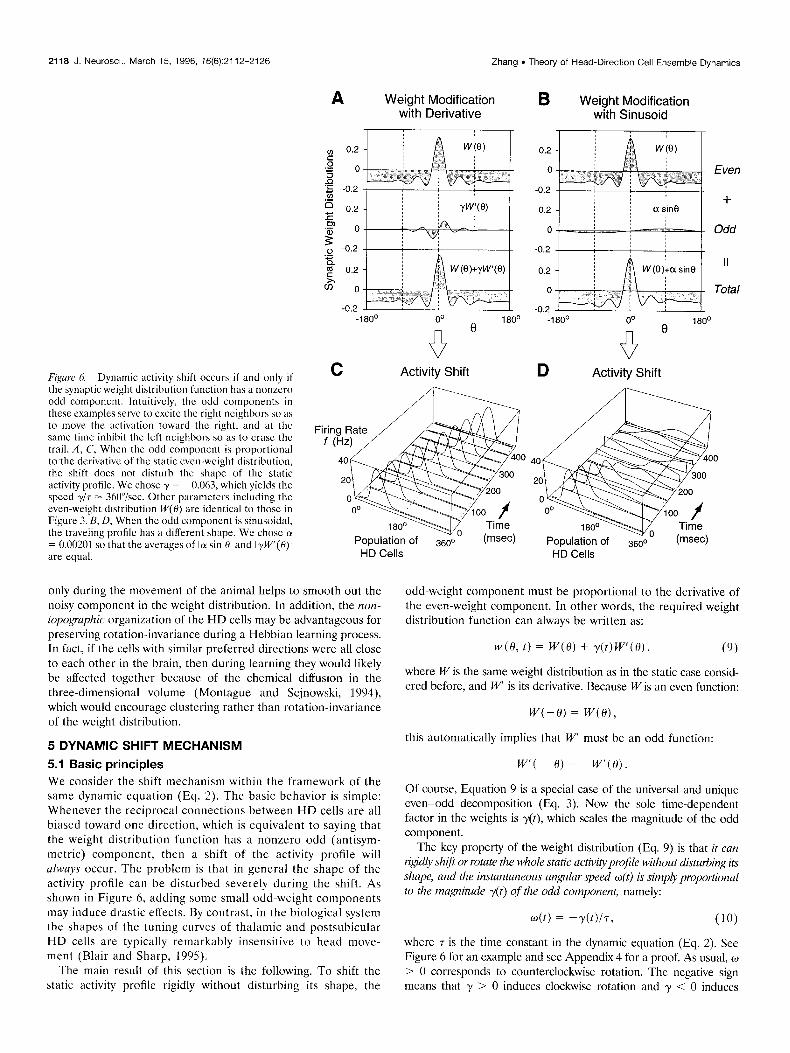
Figure 6. Dynamic activity shift occurs if and only il

A Weight Modification with Derivative

2 0.2

.o 3 0 0 Even 9 z -0.2 -0.2 +

; asine

B Weight Modification with Sinusoid

C Activity Shift the synaptic weight distribution function has a nonzero odd component. Intuitively, the odd components in these examples serve to cxcitc the right neighbors so as to move the activation toward the right, and at the same time inhibit the left neighbors so as to crasc the trail. A, C, When the odd component is proportional to the derivative of the static cvcn-weight distribution, the shift does not disturb the shape of the static activity profile. We chose y = -0.063, which yields the speed $7 = 3hO”isec. Other parameters including the even-weight distribution W(H) are identical to those in Figure 3. B, D, When the odd component is sinusoidal, the traveling profile has a different shape. We chose 01 = 0.00201 so that the averages of Ia sin 01 and I$V’(0)l are equal.

Odd

-1800 00 0

180'

0

HD Cells

only during the movement of the animal helps to smooth out the noisy component in the weight distribution. In addition, the PZOPZ- topographic organization of the HD cells may be advantageous for preserving rotation-invariance during a Hebbian learning process. In fact, if the cells with similar preferred directions were all close to each other in the brain, then during learning they would likely be affected together because of the chemical diffusion in the three-dimensional volume (Montague and Sejnowski, 3 994), which would encourage clustering rather than rotation-invariance of the weight distribution.

5 DYNAMIC SHIFT MECHANISM

5.1 Basic principles We consider the shift mechanism within the framework of the same dynamic equation (Eq. 2). The basic behavior is simple: Whenever the reciprocal connections between HD cells are all biased toward one direction, which is equivalent to saying that the weight distribution function has a nonzero odd (antisymmetric) component, then a shift of the activity profile will always occur. The problem is that in general the shape of the activity profile can be disturbed severely during the shift. As shown in Figure 6, adding some small odd-weight components may induce drastic effects. By contrast, in the biological system the shapes of the tuning curves of thalamic and postsubicular HD cells are typically remarkably insensitive to head movement (Blair and Sharp, 199.5).

The main result of this section is the following. To shift the static activity profile rigidly without disturbing its shape, the

18

Population of HD Cells

360'

Time (msec)

odd-weight component must be proportional to the derivative of the even-weight component. In other words, the required weight distribution function can always be written as:

w(@, t) = w(e) + y(t)W’(fQ, (9)

where W is the same weight distribution as in the static case considered before, and w’ is its derivative. Because W is an even function:

W(-0) = W(O),

this automatically implies that W’ must be an odd function:

W’( - 0) = -W’(O).

Of course, Equation 9 is a special case of the universal and unique even-odd decomposition (Eq. 3). Now the sole time-dependent factor in the weights is y(t), which scales the magnitude of the odd component.

The key property of the weight distribution (Eq. 9) is that it can rigidly shif or rotate the whole static activityprofile without disturbing its shape, and the instantaneous angular speed o(t) is simply proportional to the magnitude y(t) of the odd component, namely:

o(t) = -y(t)/7, (10)

where 7 is the time constant in the dynamic equation (Eq. 2). See Figure 6 for an example and see Appendix 4 for a proof. As usual, w > 0 corresponds to counterclockwise rotation. The negative sign means that y > 0 induces clockwise rotation and y < 0 induces

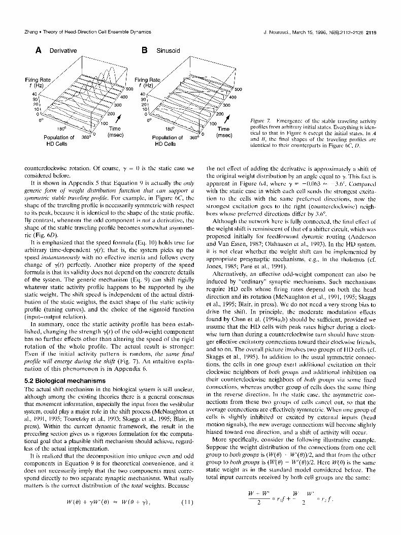
Zhang . Theory of Head-Direction Cell Ensemble Dynamics J. Neurosci., March 15, 1996, 76(6):2112-2126 2119

A Derivative B Sinusoid

Hb Cells Hb Cells

counterclockwise rotation. Of course, y = 0 is the static case we considered before.

It is shown in Appendix 5 that Equation 9 is actually the OY+ generic form of weight distribution function that cun .support (I symmetric stuhle truveling profile. For cxamplc, in Figure hC, the shape of the traveling profile is necessarily symmetric with respect to its peak, bccausc it is identical to the shape of the static profile. By contrast, whenever the odd component is not a dcrivativc, the shape of the stable traveling profile becomes somewhat asymmetric (Fig. hD).

It is emphasized that the speed formula (Eq. 10) holds true for arbitrary time-dcpendcnt r(t); that is, the system picks up the speed instuntaneously with no effective inertia and follows every change of y(t) perfectly. Another nice property of the speed formula is that its validity does not depend on the concrete details of the system. The generic mechanism (Eq. 9) can shift rigidly whatever static activity profile happens to be supported by the static weight. The shift speed is independent of the actual distribution of the static weights, the exact shape of the static activity profile (tuning curves), and the choice of the sigmoid function (input-output relation).

In summary, once the static activity profile has been established, changing the strength y(t) of the odd-weight component has no further effects other than altering the speed of the rigid rotation of the whole profile. The actual result is stronger: Even if the initial activity pattern is random, the same final profile will emerge during the shift (Fig. 7). An intuitive expla- nation of this phcnomcnon is in Appendix 6.

5.2 Biological mechanisms The actual shift mechanism in the biological system is still unclear, although among the existing thcorics there is a general consensus that movement information, especially the input from the vestibular system, could play a major role in the shift process (McNaughton et al., 1991, 199.5; Touretzky et al., 1993; Skaggs et al., 1995; Blair, in press). Within the current dynamic framework, the result in the preceding section gives us a rigorous formulation for the computational goal that a plausible shift mechanism should achieve, regardless of the actual implementation.

It is realized that the decomposition into unique even and odd components in Equation 9 is for theoretical convenience, and it does not necessarily imply that the two components must corre- spond directly to two separate synaptic mechanisms. What really matters is the correct distribution of the total weights. Because

W(0) + yW’(0) = W(0 + y), (11)

Firi f

F@r-e 7. Emcrgcnce of the stable travcliq activity profiles from arbitrary initial states. Everything is identical to that in Figure 6 except the initial states. In A and B, the final shapes of the travelin!: profiles are identical to their c&tcrparts in Figul-c%i’, D.

the net effect of adding the derivative is approximately a shift of the original weight distribution by an angle equal to y. This fact is apparent in Figure (,A, whcrc y = -0.063 = -3.0”. Compared with the stalic cast in which each ccl1 sends the strongest cxcita- tion to the cells with the same prcfcrrcd directions, now the strongest excitation goes to the right (countcrclockwisc) ncigh- bors whose prcfcrrcd directions ditfcr by 3.6”.

Although the network hcrc is fully conncctcd. the final ctt’cct of the weight shift is reminiscent of that of a shifter circuit, which was proposed initially for feedforward dynamic routing (Anderson and Van Essen, 1987; Olshauscn ct al., 1993). In the HD system, it is not clear whether the weight shift can be implemented by appropriate presynaptic mechanisms, e.g., in the thalamus (cf. Jones, 1985; Par6 et al., 1991).

Alternatively, an effective odd-weight component can also be induced by “ordinary” synaptic mechanisms. Such mechanisms require HD cells whose firing rates depend on both the head direction and its rotation (McNaughton et al., 1991, 1995; Skaggs et al., 1995; Blair, in press). We do not need a very strong bias to drive the shift. In principle, the moderate modulation effects found by Chen et al. (1994a,b) should be sufficient, provided we assume that the HD cells with peak rates higher during a clockwise turn than during a counterclockwise turn should have stronger effective excitatory connections toward their clockwise friends, and so on. The overall picture involves two groups of HD cells (cf. Skaggs et al., 1995). In addition to the usual symmetric connections, the cells in one group cxcrt additional excitation on their clockwise neighbors of both groups and additional inhibition on

their counterclockwise neighbors of both grq~,s via some fixed connections, whereas another group of cells does the same thing in the reverse direction. In the static cast, the asymmetric con-

nections from these two groups of cells cancel out, so that the average connections are effectively symmetric. When one group of cells is slightly inhibited or excited by external inputs (head motion signals), the new average connections will become slightly biased toward one direction, and a shift of activity will occur.

More specifically, consider the following illustrative example. Suppose the weight distribution of the connections from one cell group to both groups is (w(0) + l+“(0))/2, and that from the other group to both groups is (w(0) - w’(0))/2. Here W(H) is the same static weight as in the standard model considered before. The total input currents received by both cell groups arc the same:


The trick is that now the firing rates of the two groups are modulated separately by the coefficients rl and r,. In the static case, r, = r2 = 1; that is, the hvo groups have equal firing rates, and the total input simply equals W *J This means that the overall effective weight distribution of the hvo groups is just W (symmetric) if the head does not move. During head movement, we suppose the firing rate of one group is slightly increased, whereas that of the other is slightly decreased, say, r1 = 1 + y and r, = 1 - y, then the total input becomes (W + yw’) *t In other words, the average effective weight distribution becomes W + yw’, which is precisely what is needed for the shift mechanism.

In short, although now the system consists of two groups of cells, its average behaviors during dynamic shift are identical to the standard model considered in the preceding section. Notice that only a small percentage of firing-rate modulation will be sufficient to move the activity lump at realistic turning speeds. So far the modulation of firing rates has been formulated simply as multiplicative coefficients. If the modulation is formulated as additive terms (by adding external current injection), the average behaviors of the system are no longer identical to the standard model. Simulation shows that the shapes of the traveling profiles will become slanted, especially at high speeds, with a tendency for the peak to bend in the direction opposite to the traveling direction.

In general, all we need for the activity shift is to induce some weak anisotropy in the effective connections, presumably by vestibular inputs. Although many mechanisms are possible, the final net effect must be close to Equation 9. In addition, Hebbian-type plasticity might serve to ensure the structural stability of the system (cf. Appendix 2). For fine-tuning of the shift speed, the system also needs teaching signals obtained from sources other than the vestibular input itself, perhaps including the direct retinal projections to the AD nucleus (Itaya et al., 1986).

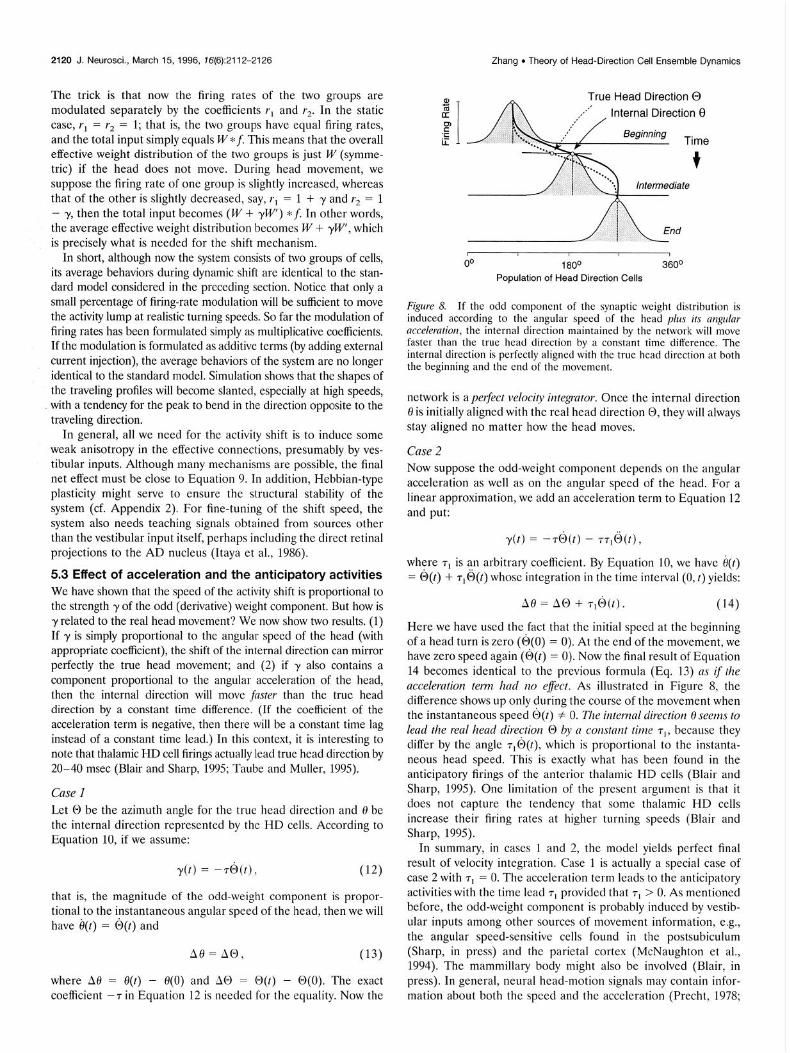
5.3 Effect of acceleration and the anticipatory activities We have shown that the speed of the activity shift is proportional to the strength y of the odd (derivative) weight component. But how is y related to the real head movement? We now show two results. (1) If y is simply proportional to the angular speed of the head (with appropriate coefficient), the shift of the internal direction can mirror perfectly the true head movement; and (2) if -y also contains a component proportional to the angular acceleration of the head, then the internal direction will move faster than the true head direction by a constant time difference. (If the coefficient of the acceleration term is negative, then there will be a constant time lag instead of a constant time lead.) In this context, it is interesting to note that thalamic HD cell firings actually lead true head direction by 20-40 msec (Blair and Sharp, 1995; Taube and Muller, 1995).

Case 1 Let 0 be the azimuth angle for the true head direction and 0 be the internal direction represented by the HD cells. According to Equation 10, if we assume:

y(t) = -76(t), (12)

that is, the magnitude of the odd-weight component is proportional to the instantaneous angular speed of the head, then we will have e(t) = b(t) and

118 = A@, (13)

where A6’ = 19(t) - 0(O) and A@ = O(t) - O(0). The exact coefficient -T in Equation 12 is needed for the equality. Now the

True Head Direction 0 Internal Direction 8

I I

00 1 80° 360”


Figtire 8. If the odd component of the synaptic weight distribution is induced according to the angular speed of the head plus its mgular acceleration, the internal direction maintained by the network will move faster than the true head direction by a constant time difference. The internal direction is perfectly aligned with the true head direction at both the beginning and the end of the movement.

nehvork is a perfect velocity integrator. Once the internal direction 8 is initially aligned with the real head direction 0, they will always stay aligned no matter how the head moves.

Case 2

Now suppose the odd-weight component depends on the angular acceleration as well as on the angular speed of the head. For a linear approximation, we add an acceleration term to Equation 12 and put:

y(t) = -76(t) - 77,0(t),

where T, is an arbitrary coefficient. By Equation 10, we have e(t) = o(t) + T,@(t) whose integration in the time interval (0, t) yields:

be = A0 + T&t). (14)

Here we have used the,fact that the initial speed at the beginning of a head turn is zero (O(0) = 0). At the end of the movement, we have zero speed again (6(t) = 0). Now the final result of Equation 14 becomes identical to the previous formula (Eq. 13) 11s if the acceleration term hod no @ect. As illustrated in Figure 8, the difference shows up only during the course of the movement when the instantaneous speed 6(t) # 0. The internal direction 8 seems to

lead the real head direction 0 by a constant time r,, because they differ by the angle -r,@(t), which is proportional to the instantaneous head speed. This is exactly what has been found in the anticipatory firings of the anterior thalamic HD cells (Blair and Sharp, 1995). One limitation of the present argument is that it does not capture the tendency that some thalamic HD cells increase their firing rates at higher turning speeds (Blair and Sharp, 1995).

In summary, in cases 1 and 2, the model yields perfect final result of velocity integration. Case 1 is actually a special case of case 2 with T, = 0. The acceleration term leads to the anticipatory activities with the time lead T, provided that TV > 0. As mentioned before, the odd-weight component is probably induced by vestibular inputs among other sources of movement information, e.g., the angular speed-sensitive cells found in the postsubiculum (Sharp, in press) and the parietal cortex (McNaughton et al., 1994). The mammillary body might also be involved (Blair, in press). In general, neural head-motion signals may contain information about both the speed and the acceleration (Precht, 1978;


f (Hz):

t = 0 msec t = 400 msec t = 800 msec

1.25 mlsec

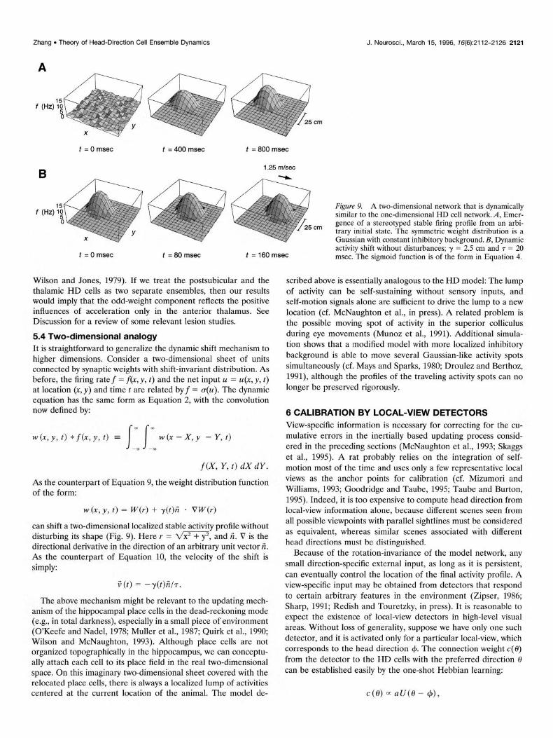
f (Hz): Figure 9. A two-dimensional network that is dynamically similar to the one-dimensional HD cell network. A, Emer- gence of a stereotyped stable firing profile from an arbitrary initial state. The symmetric weight distribution is a Gaussian with constant inhibitory background. B, Dynamic

t = 0 msec t = 80 msec t = 160msec activity shift without disturbances; y = 2.5 cm and r = 20 msec. The sigmoid function is of the form in Equation 4.

Wilson and Jones, 1979). If we treat the postsubicular and the scribed above is essentially analogous to the HD model: The lump thalamic HD cells as two separate ensembles, then our results of activity can be self-sustaining without sensory inputs, and would imply that the odd-weight component reflects the positive self-motion signals alone are sufficient to drive the lump to a new influences of acceleration only in the anterior thalamus. See location (cf. McNaughton et al., in press). A related problem is Discussion for a review of some relevant lesion studies. the possible moving spot of activity in the superior colliculus

5.4 Two-dimensional analogy during eye movements (Munoz et al., 1991). Additional simula-

It is straightforward to generalize the dynamic shift mechanism to tion shows that a modified model with more localized inhibitory

higher dimensions. Consider a two-dimensional sheet of units background is able to move several Gaussian-like activity spots

connected by synaptic weights with shift-invariant distribution. As simultaneously (cf. Mays and Sparks, 1980; Droulez and Berthoz,

before, the firing rate f = f(x, y, t) and the net input u = U(X, y, t) 1991), although the profiles of the traveling activity spots can no

at location (x, y) and time t are related by f = 4(u). The dynamic longer be preserved rigorously.

equation has the same form as Equation 2, with the convolution now defined by: 6 CALIBRATION BY LOCAL-VIEW DETECTORS

m m

\I

View-specific information is necessary for correcting for the cu-

w k y, t) * f CG y, t) = w(x-x,y -Y,t) mulative errors in the inertially based updating process consid- -m -cc ered in the preceding sections (McNaughton et al., 1993; Skaggs

et al., 1995). A rat probably relies on the integration of self- f (X, Y, t) fix dY. motion most of the time and uses only a few representative local

As the counterpart of Equation 9, the weight distribution function views as the anchor points for calibration (cf. Mizumori and

of the form: Williams, 1993; Goodridge and Taube, 1995; Taube and Burton, 1995). Indeed, it is too expensive to compute head direction from

w (x, y, t) = W(r) + y(t)2 - VW(r) local-view information alone, because different scenes seen from

can shift a two-dimensional localized stable activity profile without all possible viewpoints with parallel sightlines must be considered

disturbing its shape (Fig. 9). Here I = w, and 2. V is the as equivalent, whereas similar scenes associated with different

directional derivative in the direction of an arbitrary unit vector 2. head directions must be distinguished.

As the counterpart of Equation 10, the velocity of the shift is Because of the rotation-invariance of the model network, any

simply: small direction-specific external input, as long as it is persistent, can eventually control the location of the final activity profile. A

i; (t) = -y(t)jl/7. view-specific input may be obtained from detectors that respond

The above mechanism might be relevant to the updating mech- to certain arbitrary features in the environment (Zipser, 1986;

anism of the hippocampal place cells in the dead-reckoning mode Sharp, 1991; Redish and Touretzky, in press). It is reasonable to

(e.g., in total darkness), especially in a small piece of environment expect the existence of local-view detectors in high-level visual

(O’Keefe and Nadel, 1978; Muller et al., 1987; Quirk et al., 1990; areas. Without loss of generality, suppose we have only one such

Wilson and McNaughton, 1993). Although place cells are not detector, and it is activated only for a particular local-view, which

organized topographically in the hippocampus, we can conceptu- corresponds to the head direction 4. The connection weight c(0)

ally attach each cell to its place field in the real two-dimensional from the detector to the HD cells with the preferred direction 0

space. On this imaginary two-dimensional sheet covered with the can be established easily by the one-shot Hebbian learning: relocated place cells, there is always a localized lump of activities centered at the current location of the animal. The model de- c(O) lx uU(B - 4),


A B From HD Celf.s

C

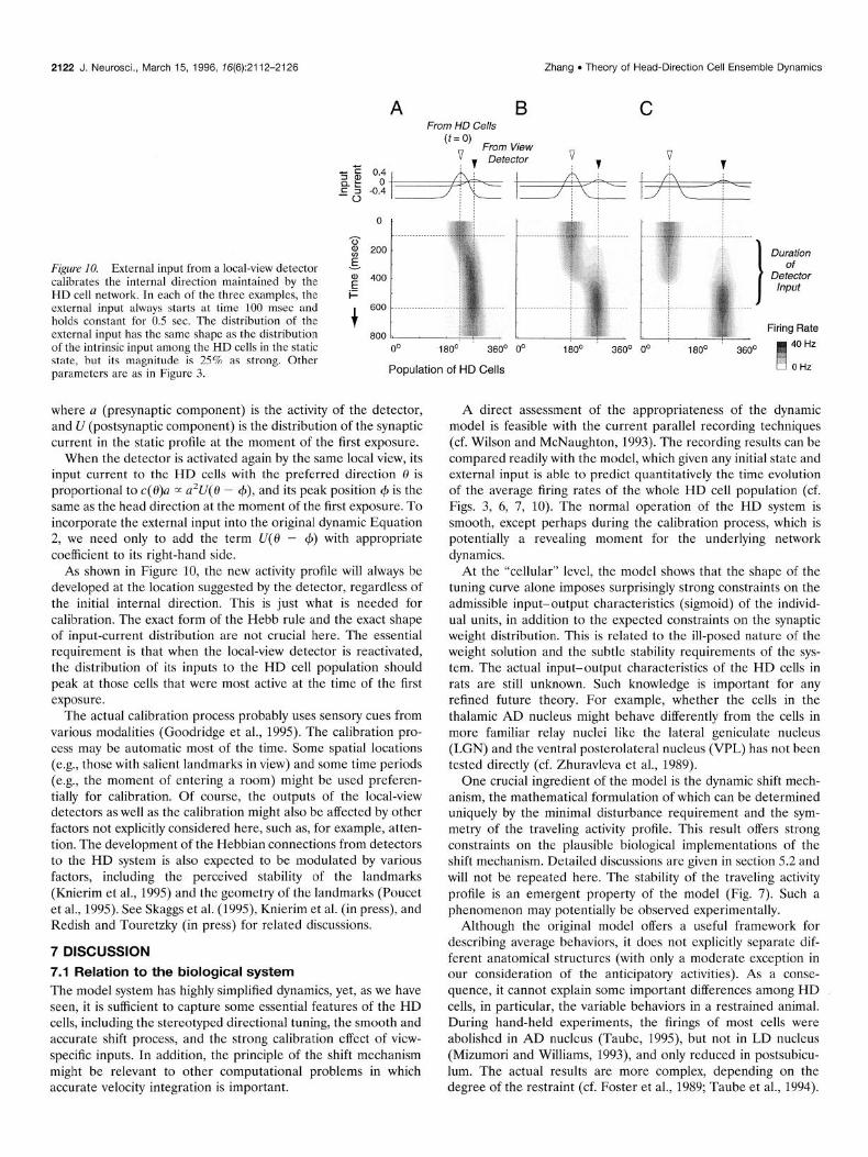
Figure 10. External input from a local-view detector calibrates the internal direction maintained by the HD cell network. In each of the three examples, the external input always starts at time 100 msec and holds constant for 0.5 sec. The distribution of the external input has the same shape as the distribution of the intrinsic input among the HD cells in the static state, but its magnitude is 25% as strong. Other parameters are as in Figure 3.

600

where a (presynaptic component) is the activity of the detector, and U (postsynaptic component) is the distribution of the synaptic current in the static profile at the moment of the first exposure.

When the detector is activated again by the same local view, its input current to the HD cells with the preferred direction 8 is proportional to c( @)a m a’U( 0 - +), and its peak position (p is the same as the head direction at the moment of the first exposure. To incorporate the external input into the original dynamic Equation 2, we need only to add the term U(0 - 4) with appropriate coefficient to its right-hand side.

As shown in Figure 10, the new activity profile will always be developed at the location suggested by the detector, regardless of the initial internal direction. This is just what is needed for calibration. The exact form of the Hebb rule and the exact shape of input-current distribution are not crucial here. The essential requirement is that when the local-view detector is reactivated, the distribution of its inputs to the HD cell population should peak at those cells that were most active at the time of the first exposure.

The actual calibration process probably uses sensory cues from various modalities (Goodridge et al., 1995). The calibration process may be automatic most of the time. Some spatial locations (e.g., those with salient landmarks in view) and some time periods (e.g., the moment of entering a room) might be used preferen- tially for calibration. Of course, the outputs of the local-view detectors as well as the calibration might also be affected by other factors not explicitly considered here, such as, for example, attention. The development of the Hebbian connections from detectors to the HD system is also expected to be modulated by various factors, including the perceived stability of the landmarks (Knierim et al., 1995) and the geometry of the landmarks (Poucet et al., 1995). See Skaggs et al. (1995), Knierim et al. (in press), and Redish and Touretzky (in press) for related discussions.

7 DISCUSSION 7.1 Relation to the biological system The model system has highly simplified dynamics, yet, as we have seen, it is sufficient to capture some essential features of the HD cells, including the stereotyped directional tuning, the smooth and accurate shift process, and the strong calibration cffcct of vicw- specific inputs. In addition, the principle of the shift mechanism might be relevant to other computational problems in which accurate velocity integration is important.

of Detector Input

Firing Rate

40 Hz

Population of HD Cells 0 Hz

A direct assessment of the appropriateness of the dynamic model is feasible with the current parallel recording techniques (cf. Wilson and McNaughton, 1993). The recording results can be compared readily with the model, which given any initial state and external input is able to predict quantitatively the time evolution of the average firing rates of the whole HD cell population (cf. Figs. 3, 6, 7, 10). The normal operation of the HD system is smooth, except perhaps during the calibration process, which is potentially a revealing moment for the underlying network dynamics.

At the “cellular” level, the model shows that the shape of the tuning curve alone imposes surprisingly strong constraints on the admissible input-output characteristics (sigmoid) of the individual units, in addition to the expected constraints on the synaptic weight distribution. This is related to the ill-posed nature of the weight solution and the subtle stability requirements of the system. The actual input-output characteristics of the HD cells in rats are still unknown. Such knowledge is important for any refined future theory. For example, whether the cells in the thalamic AD nucleus might behave differently from the cells in more familiar relay nuclei like the lateral geniculate nucleus (LGN) and the ventral posterolateral nucleus (VPL) has not been tested directly (cf. Zhuravleva et al., 1989).

One crucial ingredient of the model is the dynamic shift mechanism, the mathematical formulation of which can be determined uniquely by the minimal disturbance requirement and the symmetry of the traveling activity profile. This result offers strong constraints on the plausible biological implementations of the shift mechanism. Detailed discussions are given in section 5.2 and will not be repeated here. The stability of the traveling activity profile is an emergent property of the model (Fig. 7). Such a phenomenon may potentially be observed experimentally.

Although the original model offers a useful framework for describing average behaviors, it does not explicitly separate different anatomical structures (with only a moderate exception in our consideration of the anticipatory activities). As a consequence, it cannot explain some important differences among HD cells, in particular, the variable behaviors in a restrained animal. During hand-held experiments, the firings of most cells were abolished in AD nucleus (Taube, 1995), but not in LD nucleus (Mizumori and Williams, 1993), and only reduced in postsubiculum. The actual results are more complex, depending on the degree of the restraint (cf. Foster et al., 1989; Taube et al., 1994).


Preliminary reports of lesion studies by Taube and colleagues revealed other interesting differences. For example, postsubicular HD cells vanished after lesions to the AD nucleus (Goodridge and Taube, 1993) but not to the LD nucleus (Golob and Taube, 1994). Conversely, some thalamic HD cells still could be found after lesions to the postsubiculum (Goodridge and Taube, 1994). The activities of thalamic HD cells were severely disrupted by vestibular lesions (Stackman and Taube, 1995). So it seems that the thalamic HD cells can survive without postsubiculum, but not the other way around. If we assume as before that the directional tuning curves (and HD cells) are a network property, and that the very existence of HD cells relies on an intact dynamic shift mechanism, then the lesion data may suggest that the thalamic HD cells are related more directly to the shift mechanism, whereas the postsubicular HD cells are not. This does not necessarily imply that the postsubicular cells cannot influence the thalamic cells. For example, the postsubiculum might be more involved with the calibration process or the recognition of local views. The current model clearly needs to be extended to incorporate those phenomena explicitly involving different anatomical structures.

Finally, as a simple generalization of the current model, WC can separate the excitatory (HD) cells and the inhibitory cells and assume that the inhibitory cells are not tuned to head direction:

where f,, = v,..(u,,) and f,,, = pin(uin), andf,,(t) is the average of f,,(0, t) over all directions. The excitatory and inhibitory popula- tions are coupled by the connections Ci, and C,,. Compared with the original model, the major difference is that the overall inhibitory level here is adjustable according to the activities of the HD cells. This does not change the static activity profile or the shift mechanism, however, because the average activation keeps constant in both cases.

7.2 Relation to human perception The properties of the HD cells in rats are remarkably consistent with our own internal experiences or our common sense about the subjective sense of orientation. We seldom notice the existence of our sense of direction until it goes wrong. Disorientation often occurs after people ride passively in a vehicle, unaware of a slow turn. An important property revealed by the disorientation experiences is that without the help of familiar landmarks, one can hardly reset the internal direction at will, despite one’s conscious knowledge of the error based on other cues, e.g., the expected position of the sun. Another phenomenon is less frequent but more dramatic. In approaching a place with salient landmarks that was seen initially with an incorrect sense of direction, the currently correct sense of direction can suddenly flip back to the wrong orientation again when the landmarks are recognized, in what can feel like a sudden vertiginous rotation of the whole world (Jon- sson, 1993, and the references therein).

All these phenomena can be explained naturally if we assume that HD cells similar to the ones found in rats also exist in humans and that the subjective sense of orientation is determined by the preferred directions of the currently active HD cells. In particular, the switching of HD-cell preferred directions between conflicting environments (Goodridge and Taube, 1995; Taube and Burton, 1995) is an excellent animal model for the human phenomenon described by Jonsson (1993). Although HD cells may well exist in

other species, recording experiments on freely moving animals have been performed most successfully in rats. The possible existence of HD cells in the homologous brain regions in other species has not been tested directly, although recent experiments in monkeys did reveal some view-dependent spatial representations in the hippocampus (Ono et al., 1993; Rolls et al., 1995).

APPENDIX

1. Directional tuning curve First notice that for realistic values of the parameters, the tuning function (Eq. 1) is very close to an ordinary Gaussian even though it is periodic, whereas a Gaussian is not. In fact, by Taylor expansion:

which is a Gaussian with the standard deviation l/, K. The deviation may be used to characterize the width of the tuning curve. For example, to compare with the paramctcrs of the triangular model (Taube et al., 199Oa; Taube, 19%). WC: can obtain a triangle by drawing tangent lines at the two inflection points (ic., points with vanishing second derivatives) of the Gaus-

sian curve; then the width of the base at the lcvcl of the background firing rate is just 41 JK. In other words:

directional firing range(or base width) - 230”/ ,{K.

The firing range of a typical HD cell is roughly one quarter of the circle, which immediately gives the crude estimate K - 6.5.

Given an HD cell, the exact values of the parameters {A, B, K, 0,~) for the tuning curve can be determined by any numerical methods that yield the least mean square fit to the tuning data. Because the effectiveness of an iterative method typically depends on the initial values of the parameters, a quick good estimate is desirable. In the data, let fmin be the background firing rate, f,,, the peak rate, and f,,,,,, the mean rate over all directions, then:

The first formula follows from the exact equationf,,,,;,,, = 112~ S$m f d0 = A + B&,(K) and the approximation I,,(K) = 8/ \%kK, where I,,(K) is a Bessel function of zero order of imaginary argument.

2. Learning the synaptic weights The weight distribution solved by regularization in section 4.3 can be learned by adjusting the weights according to the gradient of the error function (Eq. 6). This procedure is basically a delta rule with weight decay, and the level of regularization is controlled by the rate of the decay. (A modified learning rule with either the pre- or postsynaptic activation replaced by the corresponding time derivative can learn the derivative of the static weight distribution, which is related to the shift mechanism.)

First, it is helpful to see how a simple Hebb rule should be formulated in a rotation-invariant system. Let w(H,, 0,) be the average weight for the connections from the units with preferred direction 0, to the units with preferred direction &. Consider the


ordinary simple H&b rule with arbitrary pre- and postsynaptic activation functions:

Assuming that the learning process is the same for all directions, we put H = iY2 - 0, and write w(&, 0,) = ~(0~ - 0,) = w(0), which is just the average weight distribution function defined before. Averaging over 0, gives the overall weight change:

$(B)“& I Post (0 + BJPre (OJdO, = Post (0) * Pre (f3).

In the last step we used the assumption that Pre and Post are even functions. Thus, in a rotation-invariant system with symmetric Pre and Post activation functions, the simple Hebb rule has the form Post * Pre, with *: indicating convolution.

Taking gradient descent of the error function (Eq. h), we have:

iJt 7: Au *f - hw, (15)

where

We can identify Au with Post andfwith Pre. The additional linear weight decay term -Aw is responsible for the regularization.

Formula 15 is essentially a delta rule rather than a Hebb rule because the learning is supervised. Here we need to assume that the desired tuning curvef(fI) and the corresponding current ~(0) are present constantly during the training while the weights are being adjusted according to Formula 15, starting from arbitrary initial weights. The correct training activity pattern is possible only with the help of external inputs (e.g., from the sensory system), which only excite subsets of HD cells. Otherwise, if we use whatever activity profile that is currently stable as the training profile, then weight distribution will tend to spread and flatten. Furthermore, the convolution in Formula 15 requires implicitly that the peak position of the training activity profile be distributed uniformly in all directions. When the distribution of the peak positions in the actual training set is not uniform, the learned weight patterns may not be strictly rotation-invariant. This problem can be alleviated if we assume that the synaptic plasticity occurs mainly during the head movement of the animal (set section 4.5).

3. Local stability of static activity profile We want to derive the stability conditions for any given static activity profile. Let U(H) bc any stationary solution of the dynamic Equation 2; that is, U = w * o(U). We slightly perturb the stationary solution by adding an arbitrary but small function 9. We set u( 0, t) = U( 0) + q( 8, t) and linearize the original Equation 2 around U. The result is the linear system:

where 2 is a linear operator defined by

The stationary solution U is locally stable if and only if q always approaches zero, which is equivalent to that

Reh,, < 1 (17)

for all eigenvalues A,, of the linear operator Y’. As a special case, let U(0) = C be a constant (flat state), then

C = WV(C), where W is the average of w( 0). After C is solved, the linear operator 2 in Equation 16 becomes 2~ = cr’(C)w * q. The eigenvalues of the linear operator w * are equal to the Fourier coefficients I+,, of w. Thus the stability conditions (Eq. 17) now become:

a’(C)bc,, < 1) n = 1, 2, 3, . . .

Intuitively this means that the flat state is stable only when the sigmoid is not too steep and the weights are not too strong. The system in Figure 3 violates the stability conditions (max w’(C)~,, = 1.05 > 1).

Finally, the bias in the sigmoid is not really equivalent to the background inhibition in the weight distribution. Although the simultaneous replacements w( 0) - w( 0) + w,, and U( fI) - U( 0) + w,,f leave the static equation U = w * f invariant, the stability of the stationary state in question can bc altcrcd. Hcrc w,, is an arbitrary constant and ,T is the avcragc of .f’ = CT(U).

4. Speed formula To prove the speed formula (Eq. IO), consider the full dynamic equation:

T;u(o: t) = -u(0, t) + [W(0) + y(t)W’(fl)] *f(B, t),

(18) where f = a(u) as usual. First set y = 0 and let 14 approach the stationary profile U(0). As before, we have

U(0) = W(0) *F(0), F(0) = a(U(0)).

Because

= y(t)/7, all we need to show is that

is an exact solution of the full dynamic Equation 18. Tlk is qGalent to the statement that the stationnly pwfik U(H) is heirlg rigidly rotated at the instantwwous speed - y(t)/r. We insert (Eq. 19) into the right-hand side of the dynamic equation and obtain:

-U+(W+ yW’)“F= yU’,

using W * F = U and w’ * F = (W * F)’ = U’. Here the prime unambiguously denotes the derivatives of single-variable functions. Similarly, the left-hand side becomes:

;U’++;j,;~(s)ds] =yU’

This proves that Equation 19 is an exact solution of the full dynamic Equation 18.


5. Symmetry of traveling profile and uniqueness of the shift mechanism

The symmetry of the traveling profile implies that during the dynamic shift, the weight distribution function must be of the unique form in Equation 9. To see this, we start with the constant weight distribution:

and suppose ~(0, t) = U(0 - w t) is a symmetric stable traveling profile; that is, U(-0) = U(0). On substituting ~(0, t) with U(0 - w t) in the original dynamic Equation 2 and then putting t = 0, we have:

U(0) + rU’(N = [w,“,,,(~) + ~,,‘Id(~)l * f(N:

wheref’ = (r(U) as usual, and y = -WT. Because the even or odd components on both sides of the equation should be equal, we obtain U = w,,,,, *:J’and yU’ = w ,,‘, <I *$ Comparison of the latter with derivative of the former (U’ = w:,,,, :i:,f’) leads to:

W ,,<,<, * f = yw :,,,, 4: 1’.

In general, WC can assume thatf’has broad Fourier spectrum; that is, none of its Fourier cocficicnts is exactly zero. This implies that W odd = yw:,,,,, hcncc Equation 9.

6. Discrete time approximation: iteration method Because

u(0,r+7) = u(H,t)+T:):u(H,t),

the continuous dynamical equation

7 ,“, u(0, t) = -u(@t) + W(0) * cr(u(0, t))

can be approximated by the iteration

u(H,t+7) = W(0) * cT(ll(H, t)).

So, starting from the initial state ~,~(8), the successive iteration

uk+,(H) = W(H) * a(uk(0)), k = 0, 1, 2, . . . (20)

generates a sequence

which can bc considered roughly as the snapshots of the solution of the continuous equation at the time instants 0, 7, 27, 3~, . . . , etc. If the iteration converges to a fixed point 11~ + U, then U is also an exuct stationary solution of the original continuous equation.

The iteration method gives us a simple intcrprctation of the shift mechanism. In Equation 20, replace W(0) by lY(0 + y). Then the same iteration will now yield:

UdN, u,(O + Y), 40 + 271, udfl + 3Y). . , (22)

because of the property of the convolution. Note that the time evolution processes of the two sequences (21 and 22) arc identical, except for the successively larger rotations, and the speed of the rotation is clearly $7. This rotation is related to the continuous shift mechanism (Eq. 9) by the approximation W(H + y) = w(0) + yW(0).

The equivalence of the two sequences (21 and 22) also explains

why the time course of the emergence of a stable travehg profile

(Fig. 7A) looks so similar to its counterpart of a static profile (Fig. 3A), except for the successive shifts. In fact, now the stability of the static profile implies the stability of the final traveling profile

and vice versa. One problem of the iteration method is that it

sometimes approaches a stable oscillation between two flat states,

a phenomenon that has no counterpart in the continuous system, regardless of the value of 7.

REFERENCES Amari SI (1972) Characteristics of random nets of analog neuron-like

elements. IEEE Trans Svs Man Cvbern 2:643-657. Anderson CH, Van Esscn’ DC (19i7) Shifter circuits: a computational

strategy for dynamic aspects of visual processing. Proc Nat1 Acad Sci USA 84:6297-6301.

Blair HT (lYY6) A thalamocortical circuit for computing directional heading in the rat. In: Advances in Neural Information Processing Systems 8 (Touretzky DS, Mozer MC, Hassclmo ME, cds). Cambridge. Massachusetts: MIT, in press.

Blair HT, Sharp FE (1995) Anticipatory head-dircclion cells in anlcriol thalumu~ cvidcncc for iI th;ll;lmocortical circuit that intcgratcs angulm head velocity to compute head direction. J Ncurosci lS:6260-6270.

Blair HT, Sharp PE (lYY6) Visual rind vcstibular inllucnccs on hcaJ- direction cells in the anterior thalamus of the rat. Bchav Ncurosci. in pl-““s.

Chcn LL, Lin LH, Green EJ, Barnes CA, McNaughton BL (I99-la) Head-dircc~ion cells in the rat posterior cortex. 1. Anatomical distribution and behavioral modulation. Exp Brain Rcs lOl:8-23.

Chcn LL, Lin LH, Barnes CA, McNaughton BL (1994b) Head-direction cells in the rat posterior cortex. II. Visual and idcothctic information to the directional firing. Exp Brain Rcs lOl:24-34.

Cohen MA, Grossberg S (1983) Ahsolutc stability of global pattern for- mation and parallel memory storage by compctilivc neural networks. IEEE Trans Sys Man Cybcrn 13:815-826.

Droulez J, Berthoz A (19Yl) A neural network model of scnsoritopic maps with predictive short-term memory propertics. Proc Natl Acad Sci USA 88:9653-9657.

Dudchenko P, Taube JS (1994) Correlation between head-direction cell activity and spatial behavior in a radial-arm maze. Sot Ncurosci Abstr 20:804.

Foster TC, Castro CA, McNaughton BL (1989) Spatial selectivity of rat hippocampal neurons: dependence on preparedness for movement. Science 244:1580-1582.

Gallistcl CR (1990) The organization of learning. Cambridge, Mass&u- setts: MIT.

Golob EJ, Taube JS (1994) Head direction cells rccordcd l’rom the postsubiculum in animals with lesions of the lateral dorsal thalamic nucleus. Sot Neurosci Abstr 20:X05.

Goodridgc JP, Taube JS ( 1993) Lesions of the anterior thalamic nucleus disrupt head direction cell firing in the dorsal prcsubiculum. Sot Ncu- rosci Abstr lY:7Y6.

Goodridge JP, Taubc JS (1994) The cl&t of Icsions of the postsubiculum on head direction cell tiring in the anterior thalamic nuclei. Sot Neurosci Abstr 20:805.

Goodridgc JP, Taubc JS (lY95) Prcfcrcntial USC of landmark nnviga- tional system by head direction cells in rats. Bchav Ncurosci 109:49-61.

Goodridge JP, Worboys KA, Dudchcnko P, Taube JS (1995) The rc- sponsc of head direction cells to non-visual cuts. Sot Neurosci Abstr 21:945.

Groetsch CW (1984) The theory of Tikhonov rcgularization for Fred- holm equations of the first kind. Boston: Pitman.

Hopfield JJ (1984) Neurons with graded response have collective computational properties like those of two-state neurons. Proc Nat1 Acad Sci USA 81:3088-3092.

Howard IP, Templeton WB (1966) Human spatial orientation. London: Wiley.

ltaya SK, Hoescn GWV, Benevento LA (1986) Direct retinal pathways to the limbic thalamus of the monkey. Exp Brain Rcs 61:607-613.

Johnson NL, Kotz S (1970) Continuous univariatc distributions, Vol 2. New York: Wiley.

Jones EG (1985) The thalnmus. New York: Plenum.


Jonsson L (1993) A simple model of our spatial system. In: Orientation and navigation: birds, humans and other animals. Oxford: The 1993 Confercncc of the Royal Institute of Navigation.

Knierim JJ, Kudrimoti HS, McNaughton BL (1995) Place cells, head direction cells, and the learning of landmark stability. J Neurosci 15:164X-1659.

Knierim JJ, Kudrimoti I-IS, Skaggs WE, McNaughton BL (1996) The interaction between vestibular cues and visual landmark learning in spatial navigation. In: Perception, memory, and emotion (Ono T, Mc- Naughton B, Molotchnikoff S, Rolls E, Nishijo H, eds), in press.

Markus EJ, McNaughton BL, Barnes CA, Green JC, Meltzer J (1990) Head direction cells in the dorsal presubiculum integrate both visual

.and angular velocity information. Sot Neurosci Abstr 16:441. Mays LE, Sparks DL (1980) Dissociation of visual and saccade-related

responses in superior colliculus neurons. J Neurophysiol 43:207-232. McNaughton BL, Chen LL, Markus EJ (1991) “Dead reckoning”, land-

mark learning, and the sense of direction: a neurophysiological and computational hypothesis. J Cognit Neurosci 3:190-202.

McNaughton BL, Markus EJ, Wilson MA, Knierim JJ (1993) Familiar landmarks can correct for cumulative error in the inertially based dead-reckoning system. Sot Neurosci Abstr 19:795.

McNaughton BL, Mizumori SJY, Barnes CA, Leonard BJ, Marguis M, Green EJ (1994) Cortical representation of motion during unre- strained spatial navigation in the rat. Ccrcb Cortex 4:27-39.

McNaughton BL, Knicrim JJ, Wilson MA (1995) Vector encoding and the vestibular foundations of spatial cognition: neurophysiological and computational mechanisms. In: The cognitive ncuroscicnccs (Gazza-

niga MS, ed), pp 585-595. Cambridge, Massachusetts: MIT. McNaughton BL, Barnes CA, Gerrard JL, Gothard K, Jung MW, Knierim

JJ, Kudrimoti H, Qin Y, Skaggs WE, Sustcr M, Weaver KL (1996) Deciphering the hippocampal polyglot: the hippocalnpus as a path integrating system. J Exp Biol, in press.

Mittelstaedt M-L, Mittelstaedt H (1980) Homing by path integration in a mammal. Naturwisscnschaftcn 67:566-567.

Mizumori SJY, Cooper BG (1995) Spatial representations of dorsal cau- date neurons of freely-behaving rats. Sot Neurosci Abstr 21:1929.

Mizumori SJY, Williams JD (1993) Directionally selective mnemonic properties of neurons in the lateral dorsal nucleus of the thalamus of rats. J Neurosci 13:4015-4028.

Mizumori SJY, Miya DY, Ward KE (1994) R eversible inactivation of the lateral dorsal thalamus disrupts hippocampal place representation and impairs spatial learning. Brain Res k44:16’8-174. .

Montague PR. Seinowski TJ (1994) The oredictive brain: temooral coin- cidence and temporal order in

, synaptic learning mechanisms. Learn

Memory 1:1-33. Muller RU, Kubic JL, Ranck Jr JB (1987) Spatial firing patterns of

hippocampal complex-spike cells in a fixed environment. J Neurosci 7:1935-1950.

Munoz DP, Pelisson D, Guitton D (1991) Movement of neural activity on the superior colliculus motor map during gaze shifts. Science 251:1358-1360.

O’Kccfe JM, Nadel L (1978) The hippocampus as a cognitive map. New York: Clarendon.

Olshausen BA, Anderson CH, Van Essen DC (1993) A neurobiological model of visual attention and invariant pattern recognition based on dynamic routing of information. J Neurosci 13:4700-4719.

Ono T, Nakamura K, Nishijo H, Eifuku S (1993) Monkey hippocampal neurons related to spatial and nonspatial functions. J Neurophysiol 70:1516-1529.

Pare D, Dossi RC, Stcriadc M (1991) Three types of inhibitory postsynaptic potentials generated by interneurons in the anterior thalamic complex of cat. J Ncurophysiol 66:1190-1204.

Poucet B, Cressant A, Muller RU (1995) The positional firing of place cells is controlled more strongly by cards on the wall than by 3-dimensional objects inside the arena. Sot Ncurosci Abstr 21:946.

Pouget A, Sejnowski TJ (1995) Dynamic remapping. In: The handbook of brain theory and neural networks (Arbib MA, ed), pp 335-338. Cambridge, Massachusetts: MIT.

Precht. W (1078) Neuronal operations in the vestibular system. Berlin: Springer.

Quirk GJ, Muller RU, Kubie JL (1990) The firing of hippocampal place cells in the dark depends on the rat’s recent experience. J Neurosci 10:2008-2017.

Ranck Jr JB (1985) Head-direction cells in the deep cell layer of dorsal presubiculum in freely moving rats. In: Electrical activity of the ar- chicortex, (Buzsaki G, Vanderwolf CH. eds). DD 217-220. Budaoest: AkadCmiai‘Kiado.

,, . .

Redish AD, Touretzky DS (1996) Modeling interactions of the rat’s place and head direction systems. In: Advances in neural information processing systems 8 (Touretzky DS, Mozer MC, Hasselmo ME, eds). Cambridge, Massachusetts: MIT, in press.

Rolls ET, Robertson RG, Georges-Francois P (1995) The representation of space in the primate hippocampus. Sot Neurosci Abstr 21:1494.

Sejnowski TJ (1977) Storing covariance with nonlinearly interacting neurons. J Math Biol 4:303-321.

Sharp PE (1991) Computer simulation of hippocampal place cells. Psy- chobiology 19:103-l 15.

Sharp PE (1996) Multiple spatial/behavioral correlates for cells in the rat postsubiculum: multiple regression analysis and comparison to other hippocampal areas. Cereb Cortex, in press.

Sharp PE, Green C (1994) Spatial correlates of firing patterns of single cells in the subiculum of the freely moving rat. J Neurosci 14:2339-2356.

Skaggs WE, Knierim JJ, Kudrimoti HS, McNaughton BL (1995) A model of the neural basis of the rat’s sense of direction. In: Advances in neural information processing systems 7 (Tcsauro G, Tourctzky DS. Lccn TK, eds), pp 173-180. Cambridge, Massachusetts: MIT.

Smith& F (1958) Integral equations. Cambridge: Cambridge UP. Stackman RW, Taube JS (1995) Influence of vcstibular system lesions

upon anterior thalamic head-direction ccl1 activity. Sot Ncurosc Abstt 21:94S.

Taubc JS (1003) Place cells rccordcd from the parasubiculum in frccly- moving animals. Sot Ncurosci Abstr IO:796

Taube JS (1995) Head direction cells rccordcd in the anterior thalamic nuclei of freely moving rats. J Ncurosci 15:70-X6.

Taube JS, Burton HL (1995) Head direction cell activity monitored in a

novel environment and during a cue conflict situation. J Neurophysiol 74:1953-1971.

Taube JS, Muller RU (1995) Head direction cell activity in the anterior thalamic nuclei, but not the postsubiculum, predicts the animal’s future directional heading. Sot Neurosci Abstr 21:946.

Taube JS, Muller RU, Ranck Jr JB (1990a) Head-direction cells re- corded from the postsubiculum in freely moving rats. I. Description and quantitative analvsis. J Neurosci 10:420-435.

Taube JS, Muller -RU, Ranck Jr JB (1990b) Head-direction cells re- corded from the postsubiculum in freely moving rats. II. Effects of environmental manipulations. J Neurosci 10:436-447.

Taube JS, Kesslak JP, Cotman CW (1992) Lesions of the rat postsubiculum impair performance on spatial tasks. Behav Neural Biol 57:131-143.

Taube JS, Wolk DA, Dudchenko P (1994) The effects of restraint on head direction cell activity. Sot Neurosci Abstr 20:805.

Touretzky DS, Redish AD, Wan HS (1993) Neural representation of space using sinusoidal arrays. Neural Comput 5:X69-884.

Tsodyks M, Sejnowski TJ (1095) Associative memory aind hippocampal place cells. Int J Neural Sys 6(suppl):81-86.

Vogt BA, Gabriel M (1993) Neurobiology of cingulate cortex and limbic thalamus: a comprehensive handbook. Boston: Birkhauscr.

Wiener SI (1993) Spatial and behavioral correlates of striatal neurons in rats performing a self-initiated navigation task. J Neurosci 13:3802-38 17.

Wilson MA, McNaughton BL (1993) Dynamics of the hippocampal ensemble code for space. Science 261:1055-1058. (Corrections in Vol. 264: 16.)

Wilson VJ, Jones GM (1979) Mammalian vestibular physiology. New York: Plenum.

Zhang, K-C (1995) Dynamical representation of spatial orientation: a model of head direction cells. In: Proceedings of the 2nd Joint Sympo- sium on Neural Computation, pp 24-25. University of California, San Diego, and California Institute of Technology.

Zhuravleva ZN, Pakhotin PI, Vinogradova OS (1989) Some unusual characteristics of the nucleus anterodorsali thalami: neurophysiological and ultrastructural investigation. J Hirnforschung 30:619-635.

Zipser, D (1986) Biologically plausible models of place recognition and goal location. In: Parallel distributed processing: explorations in the microstructure of cognition, Vol 2 (McClelland JL, Rumelhart DE, eds), pp 432-470. Cambridge, Massachusetts: MIT.

Documents

Representation of Spatial Orientation by the Intrinsic ...sereno/170/readings/39-HeadDirModel.pdfThe Journal of Neuroscience, March 15, 1996, 16(6):2112-2126 Representation of Spatial