Representation of Hydrodynamic Model Results through

ERDC/CHL CETN-IV-27September 2000

1

Representation of Hydrodynamic ModelResults through Graphical Displays

by Mark S. Gosselin, R. Bruce Taylor, and Kenneth R. Craig

PURPOSE: The Coastal Engineering Technical Note (CETN) described herein containsinformation and procedures for displaying hydrodynamic modeling results within the Surface-water Modeling System (SMS) platform. Such visualization facilitates the interpretation of largeamounts of complex output generated by the models, as well as assist the engineer incommunicating modeling results to laymen, planners, and others who lack expertise.

BACKGROUND: With the increasing application of numerical modeling methods bypracticing professionals, attention has shifted to enhancing the capabilities for displaying modeloutput. Methods developed by the Diagnostic Modeling System (DMS) (Kraus 2000) that aid ininterpreting physical flow features and coupling of hydrodynamics with sediment transportreceive special emphasis in this CETN. Traditional visualization techniques are reviewed,followed by more modern products that have proved their utility in support of engineeringprojects.

Traditional output formats for displaying hydraulic model results were mostly limited to blackand white flow vector plots and time-histories of water-surface elevation, current, or flow ratedischarge at selected locations of interest. Figures 1 through 3 show examples of these types ofoutput. Although helpful, they do not provide adequate insight on the flow or sedimentmovement. Flow vector plots (Figure 1), although depicting representative flow patterns of theentire system, are qualitative and heuristic. They leave the engineer with no direct means ofdistinguishing problematic flow conditions from acceptable conditions. Similarly, time-historyplots, although specific and quantitative, convey no relationship between data depicted at onelocation to the overall behavior of the system. Recent attention to graphical display of modelresults has addressed these shortcomings.

With the advancement of computer technology and graphics capabilities, more varied andcreative ways for displaying model output have begun to appear. Figures 4 through 6 showexamples, all of which represent significant improvements in diagnostic output formats. InFigure 4, overlaying the velocity vectors on a false color background of the modeled bathymetryenhances the traditional flow vector plot. This output format gives the user insight into the broadflow properties of the system and how they are controlled by bathymetry, a significant diagnosticrelationship. Figure 5 displays quantitative velocity information in a format significantlydifferent than the traditional time-history plots shown in Figures 2 and 3. Here, values ofvelocity, computed at each mesh element, generate isovels or contours of equal velocity. Bydisplaying various parameters (e.g., bathymetry, velocity) together, the user can understand theextent of specific thresholds of strong and weak currents and the relationships of these areas toshoreline orientation, structures, and bathymetry.


2

Figure 1. A traditional black and white velocity vector plot thatprovides a qualitative picture of the entire system, but not specific

causal relationships between flows and bathymetry

Figure 2. A traditional discharge time-history plot that provides point-specific,quantitative information, but fails at providing a picture of the flow conditions overthe entire domain (Volumetric flow rate is in cubic feet per second. To convert to

cubic meters per second, multiply by 0.3048)

-30,000

-20,000

-10,000

0

10,000

20,000

30,000

0 5 10 15 20 25 30 35 40

Time (hrs)

Vol

umet

ric

Flow

Rat

e (c

fs)

Q(bridge)

Q(south)

Time (hr)


3

Figure 3. A traditional elevation time-history plot that provides point-specific,quantitative information, but does not give a picture of the flow conditions

over the entire domain1

Figure 4. A false-color bathymetry filled contour plot with velocity vector overlay plot (units in ft) thatillustrates causal relationships between velocity and bathymetry

1 All elevations (el) cited herein are in feet referenced to the National Geodetic Vertical Datum(NGVD) (To convert feet to meters, multiply by 0.3048).

0

2

4

6

8

10

12

0 5 10 15 20 25 30 35 40

Time (hours)

Ele

vatio

n (f

t-N

GV

D29

)

Time (hr)

Ele

vatio

n (f

t-N

GV

D29

)

elevation

-82

-74

-66

-58

-50

-42

-34

-26

-18

-10

-2

6

14


4

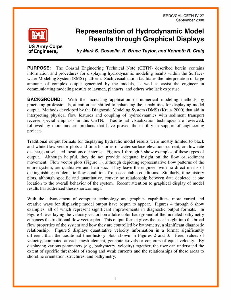
Figure 5. An isovel-filled contour plot with velocity vector overlay (units in ft/s) that provides quantitativeinformation over the entire area of interest (Velocity is in feet per second. To convert to meters per

second, multiply by 0.3048)

Finally, in Figure 6, the logic behind Figure 5 extends one step further. In this figure, contours ofchange in velocity are shown with increased velocities in red and decreased velocities in blue.These types of formats are particularly helpful for the evaluation of proposed or expectedchanges in bathymetry, channel alignment, or structural modifications. To generate this type ofplot, the hydrodynamic model must be run twice — once for baseline conditions and once for thechanged conditions under consideration. Computed velocity values for each model simulationare then overlaid to create a single new output file representing the change in velocity at eachelement. These data are then displayed, as in the contours shown in Figure 6. The color contoursreadily highlight those areas which may become prone to erosion (red) and deposition (blue)should the condition change. This CETN provides guidelines for creating plots fromhydrodynamic output, such as Figures 4 through 6, that improve the transfer of flow information,enable an improved level of understanding about the model results, and provide insight intosediment transport without having to run a time-dependent sediment transport model.

Although this CETN functions together with the DMS as a guide for identifying areas ofpersistent shoaling through graphical interpretation, the methods described herein are applicablefor displaying hydrodynamic output of any kind, including those obtained from physical models.This CETN first reviews the platform (SMS) (Brigham Young University 1999) for creating thetypes of plot presented in Figures 4 through 6, and then discusses presentation of the directhydrodynamic output. Finally, the discussion ends with methods to manipulate the output togain further insight into the flow physics and sediment transport.

velocity mag 1 : 18.500

0.14

0.70

1.26

1.82

2.38

2.94

3.50

4.06

4.62

5.18

5.74

6.30

6.86

ERDC/CHL CETN-IV-27 Revised March 2011

5

SURFACEWATER MODELING SYSTEM (SMS) FUNCTIONALITY: The SMS was

developed by the Engineering Computer Graphics Laboratory at Brigham Young University (BYU)

under sponsorship by the U.S. Army Corps of Engineers and the U.S. Federal Highway

Administration (FHWA). The SMS is a pre- and post-processor for numerous hydrodynamic

modeling programs including ADCIRC, FESWMS, RMA2, RMA4, and WSPRO. It is a pre- and

post-processor for surface-water modeling and analysis (BYU 1999). Further information about the

SMS can be located at the following address: http://chl.erdc.usace.mil/sms. This CETN discusses

only the recent (Version 7) postprocessing capability of SMS to produce an array of contour and

velocity vector plots from hydrodynamic model results. In addition, the SMS Data Calculator feature

is discussed for creating data sets that aid in discerning flow and sediment transport behavior.

The SMS contains the capability for creating contour plots of scalar data on a finite-element mesh.

Three different types of contours are available, including normal linear contours, color fill between

contours, and cubic spline contours. The user controls the number of contours, the contouring

interval, minimum and maximum contour values, labeling options, bolding contours, and the color

scale. SMS also can produce vector plots from vector data on a finite element mesh. The user

controls the arrowhead style and size, vector length, vector placement and density, and color. The

user can also vary the vector length and vector color proportionately with the velocity magnitude.

http://chl.wes.army.mil/software/sms/


6

In addition to its plot-making abilities, the SMS can construct vector data sets from scalar data,and vice versa. Also, the data calculator allows the user to manipulate multiple scalar data setswith several simple operations to form new scalar data sets. A subsequent section presents anexample of such a manipulation.

PRESENTATION OF OUTPUT: Default output from two-dimensional, depth-averaged,hydrodynamic models includes water-surface elevation and velocities — velocity magnitude as ascalar data set and speed and direction as a vector data set. In addition, model input contains abathymetry data set. The drawing of causal relationships between the bathymetry and the speedand direction is the key to understanding simulation results. Discussion will concentrate on thecreating model output plots that better illustrate these casual relationships and increaseunderstanding of the acting processes. For all subsequent figures, the example plots were createdfrom a simulation of the flow at East Pass, FL, during spring ebb tide.

A standard vector plot with an outline of the shoreline is shown in Figure 1. As shown inFigure 7, vector plots are greatly enhanced when overlaid on a false color bathymetry plot. Thecontour range is set at the limits of the bathymetry bounded by the plot rather than the entiremesh to show greater detail. In addition, the number of contours has been increased from thedefault number of 10 to 40 to show even more contrast. The legend on the left hand side hasbeen expanded from the default length, as shown in Figures 4 through 6, to span the entire heightof the plot. This expansion facilitates contour identification in working with a greater number ofcontours. The vector overlay plot includes setting the vector length proportional to the vectormagnitude. From this plot, the influence and control exerted by the local water depths arereadily seen. For example, the velocities decrease following the vertical expansion over the ebbshoal. Also, the velocities north of the spur jetty show a marked decrease, indicating that thespur functions in its capacity to deflect high velocity flows away from the shoreline north of theeast jetty. Beyond these observations, distinguishing the flow behavior in the channel is difficultgiven that the eye cannot discern the small differences in the vector lengths as water moves fromnorth to south. Another difficulty associated with this plot is discerning the flow patterns in areasof small finite elements (e.g., between the jetties). To address this difficulty, SMS contains thecapability to create a grid of vectors at a user defined spacing rather than attach the vectors toeach node. Figure 8 illustrates this capability. From this figure, one can readily discern the flowpatterns between the jetties as opposed to Figure 7 where no patterns are discernable. Thistechnique must be applied judiciously, however. Too large a grid spacing may not resolve theflow features that the modeler was trying to capture with the small elements in the first place.


7

Figure 7. Velocity vector plot overlaid on contours of bathymetry (units in ft) (Tomultiply by 0.3048)

Figure 8. Gridded velocity vector plot overlaid on contours of bathymetry (units imeters, multiply by 0.3048)

elevation

-40.0

-38.0

-36.0

-34.0

-32.0

-30.0

-28.0

-26.0

-24.0

-22.0

-20.0

-18.0

-16.0

-14.0

-12.0

-10.0

-8.0

-6.0

-4.0

-2.0

0.0

Elevation (ft)

-75.0-72.0-69.0-66.0-63.0-60.0-57.0-54.0-51.0-48.0-45.0-42.0-39.0-36.0-33.0-30.0-27.0-24.0-21.0-18.0-15.0-12.0-9.0-6.0-3.00.0

N

convert feet to meters,

n ft

Spur Jetty

N

) (To convert feet to


8

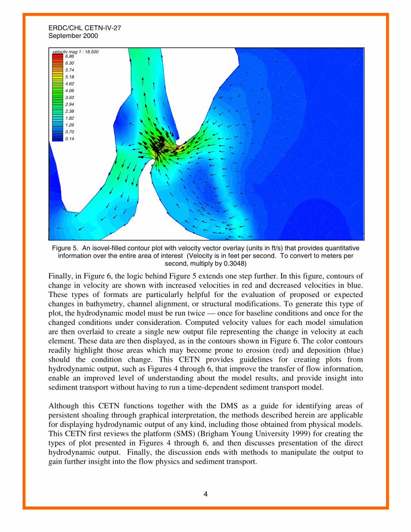
To better comprehend the velocity variation within the channel, Figure 9 illustrates a vector plotoverlaid on a contour plot of velocity magnitude. The contour plot shows many of the sametechniques discussed with the previous figure. The contour plot employs the psychologicalassociation of the cooler (blue) colors with inactivity (lower velocities) and hot colors (red) withactivity (higher velocities) by reversing the default color scale. The vector lengths were rescaled,compared to Figure 7, to display the underlying color contours. Also, the lowest magnitudevectors were set to a finite length to show behavior in regions of low velocity. Finally, thevectors were set to white to provide contrast with the darker contours.

Figure 9. Velocity vector plot overlaid on contours of velocity magnitude (units in ft/s)meters, multiply by 0.3048)

Figure 9 gives much more insight into the velocity variation in the channFigure 7. Apparent from the figure, a region of acceleration occurs at thechannel just south of the constriction. Next, flow decelerates as it enters the Before exiting, the flow accelerates again, but only on the west side of the notable feature displayed is the entrainment into the ebb jet that extends aloneither side. This feature could only be resolved by setting a minimum vector le

Figure 9, however, has lost the capability for distinguishing the cause-and-between the flow and the bathymetry. Figure 10 reintroduces this capabdisplays a gray scale contour plot of bathymetry overlaid with a velocity vectolength and color are proportional to the velocity magnitude. The velocity employs the same variation as the contours in Figure 9. Notably, the eye is diregions of interest in red. By this graphical means, the relationship bet

velocity mag 1 : 301.500

0.00

0.21

0.42

0.63

0.84

1.05

1.26

1.47

1.68

1.89

2.10

2.31

2.52

2.74

2.95

3.16

3.37

3.58

3.79

4.00

4.21

N

(To convert feet to

el as compared to north end of thewidening channel.channel. Anotherg the shoreline onngth.

effect relationshipility. The figurer plot. The vectorvector color scalerectly drawn to theween the velocity


9

magnitude and the bathymetry becomes apparent. For example, the acceleration following thenorthernmost constriction is due to a broad shoal located on the west side of the channel. Also,the acceleration located on the west side of the channel before the flow exits is attributed to theshallow water on the west side and the deep channel on the east. Figure 10 combines thedetailed magnitude information contained in Figure 9 with the bathymetry information containedin Figure 7.

Figure 10. Color velocity vector plot overlaid on contours of gray scale bathymetryconvert feet to meters, multiply by 0.3048)

MANIPULATION OF OUTPUT: Often, hydrodynamic simulations are perfengineered modifications or to evaluate shoaling or scouring trends in a parsection discusses aids that can be developed for arriving at conclusions aboucreating plots from the manipulation of the default model output.

Comparison Plots

Comparison plots allow the modeler to detect differences in solutions from twthereby evaluate the consequences of project alternatives. To illustrate thiconditions are compared with alternative spur jetty configurations; servconditions, the spur is oriented perpendicular to the eastern shore (see Figurspur is oriented parallel to the shoreline for the alternative configuration. As sthrough 10, the spur deflects the flow towards the center of the inlet; however, has formed at its tip. The alternative, shown in Figure 11, reorients the spur tflow obstruction to reduce tip scour and still protect the shoreline.

elevation

-40.0

-38.0

-36.0

-34.0

-32.0

-30.0

-28.0

-26.0

-24.0

-22.0

-20.0

-18.0

-16.0

-14.0

-12.0

-10.0

-8.0

-6.0

-4.0

-2.0

0.0

N

(units in ft) (To

ormed to evaluateticular area. Thist these actions by

o simulations ands capability, flowing as the basee 7), whereas thehown in Figures 7a large scour holeo present less of a


Figure 11. Velocity veft/s) to evaluate pro

Figure 11 shows theprevious alternatives.a plot of velocity vbaseline condition anoutput was convertedcondition mesh. Finaalternative velocity mdata set. The contovelocity associated wset was created by fiThese scalar data sealternative mesh. Thcomponents. Next, twx- and y-velocity comset was constructed baseline vector from change.

The contours revealappears to reduce thHowever, a marked

Magnitude Difference

-0.80

-0.74

-0.67

-0.61

-0.54

-0.48

-0.42

-0.35

-0.29

-0.22

-0.16

-0.10

-0.03

0.03

0.10

0.16

0.22

0.29

0.35

0.42

0.48

0.54

0.61

0.67

0.74

0.80

N

10

ctor difference plot overlaid on contours of velocity magnitude difference (units inposed reorientation of the spur jetty (To convert feet per second to meters per

second, multiply by 0.3048)

effectiveness of the alternative during the same flow conditions shown in The plot contains contours of velocity magnitude difference overlaid withector difference. The plot was constructed by first running the existingd the proposed alternative condition. To create the contours, the baseline to scatterpoint data. This data set was then interpolated onto the alternativelly, the baseline velocity magnitude scalar data set was subtracted from theagnitude data set via the SMS data calculator to create a velocity-differenceurs show this velocity difference. Positive values indicate increases inith the alternative, and negative values indicate decreases. The vector data

rst deconstructing the baseline vector data set into its x- and y-components.ts were then converted into scatterpoint data and interpolated onto thee alternative vector data set was also deconstructed into its x- and y-o scalar data sets of the difference between the alternative and the baselineponents were created via the SMS data calculator. Finally, a vector data

from the two difference data sets. The result is the subtraction of thethe alternative vector. The vector length is proportional to the magnitude of

areas of increase and decrease in velocity magnitude. The alternativee velocity magnitude near the shoreline (indicated by the blue contours).increase occurs in the velocity just west of the east jetty (indicated by red


11

contours). The vector plot shows the direction of the increase or decrease. For example, in theregion of velocity magnitude increase just west of the spur, the vectors show the increasedirected at the point where the spur meets the east jetty. An increase implies that this alternativemay experience an increase in foundation scour in this area — an unintended consequence of thisengineering alternative. Clearly, plots of this type can help identify consequences, both positiveand negative, caused by modifying existing configurations.

Sediment Transport

Often, hydrodynamic simulations are performed to gain insight into scour and depositionpatterns for a particular area. Rather than run a sediment transport model driven by thehydrodynamic model output, innovative manipulation of hydrodynamic model output canprovide this insight without having to operate a sediment transport model. Primarily, shear stressat the bed drives sediment transport. With velocity computed at peak ebb/flood as input, shearstresses can be estimated in the following manner: assuming the Manning formula applies locally(a reasonable assumption in working with the time scales of tidal flow which is quasi-steadystate), the Manning formula, in American customary units, is given by

2/13/2

n

486.1SRV = (1)

where V is the depth-averaged velocity, n is Manning’s n, R is the hydraulic radius (assumed tobe the local water depth), and S is the slope of the energy grade line. By momentumconservation, for steady state flows, the following equation applies

gRSρ=τ (2)

where τ is the shear stress at the bed, ρ is the mass density, g is gravity, R is the hydraulic radius,and S is the slope of the energy grade line. Combining Equations 1 and 2 and eliminating theslope of the energy grade line yields

3/12

2

n

486.1R

gV

= ρτ . (3)

In regions of uniform Manning’s n, creating plots of shear stress is possible within SMS.Entering Equation 3 in the data calculator yields a scalar data set that SMS can plot (Figure 12).To create vectors of shear stress, one must first assume that the shear stress acts in the directionof the velocity. Next, the velocity vector data set is deconstructed into scalar data sets of velocitydirection and magnitude. Finally, the shear stress vector data set is constructed by combining theshear stress magnitude scalar data set and the velocity direction scalar data set. The vectors inFigure 12 are proportional to the shear stress magnitude.


12

Figure 12. Contours of shear stress overlaid with shear stress vectors (units in

Figure 12 clearly shows the regions of increased shear stress (in red) and thus inctransport. The combination of high velocity and shallow water over the west intechannel at both the north and south end and over the ebb shoal cause large sheabed.

Calculating the sediment transport directly via a total load function produces aassessment of sediment transport. Figure 13 shows contours of sediment transcalculated with the Ackers-White (1973) total load formula. To perform thvelocities computed by the hydrodynamic model were written to an ASCII file. transport was calculated by the following equation:

mp

s

A

AFC

u

V

d

D

Vd

Q

−

= 1

*

35

where Qs is the time mean sediment transport rate of the sediment, d is the localfriction velocity, and D35 is the sediment diameter for which 35 percent ocomprising the bed is finer by weight. The variables p, m, F and A are functionssediment parameters as defined subsequently. The parameter F is given by the eq

Shear Stress

0.0000

0.0032

0.0064

0.0096

0.0128

0.0160

0.0192

0.0224

0.0256

0.0288

0.0320

0.0352

0.0384

0.0416

0.0448

0.0480

0.0512

0.0544

0.0576

0.0608

0.0640

0.0672

0.0704

0.0736

0.0768

0.0800

N

lbs/ft2)

reased sedimentrior shoal in ther stresses at the

more rigorousport magnitudee calculations,

Next, sediment

(4)

depth, u* is thef the sediment of the flow anduation


13

( )[ ] 2/135

*

1

35

110ln46.2

gDs

u

D

d

VF

p

p

−

=

−

(5)

where s is the sediment specific gravity. In addition, if

( ) 35

3/1

2* 1 Dg

sD

ν−= (6)

where ν is the kinematic viscosity, then for D* > 60

025.0

5.1

17.0

0

1 ====

C

m

A

p

(7)

and for 1<D* ≤ 60

[ ]13.8)(ln434.0ln86.2exp

34.166.9

14.023.0

ln243.01

2**1

*

*

*

−−=

+=

+=

−=

DDC

Dm

DA

Dp

(8)

This scalar data set is then read back into SMS to create the contour plot seen in Figure 13.Notably, entering a simpler total load sediment transport formula into the data calculator willcreate the similar data set.


14

Figure 13. Contours of sediment transport overlaid with sediment transport vectorsconvert cubic feet per second to cubic meters per second, multiply by 0.0

The vector data set is constructed in the same manner as the shear stress veone must assume that sediment transport acts in the same direction as the velocity vector data set is reduced into velocity-magnitude and velocity-direcFinally, the velocity direction and sediment transport magnitude scalar data sconstruct the sediment transport vector data set.

Figure 13 makes apparent regions of considerable sediment transport (in rehighlights the same regions as in previous plots –at the north and south extrover the western shoal and over the outer bar of the ebb shoal. In interpretingplots, one must read the gradients of sediment transport in the direction of sinfer bed elevation change. For example, as water flows from regionstransport to regions of strong sediment transport, scouring of the bed occustrong sediment transport because more sediment leaves the area downstreaupstream. Conversely, as water flows from regions of strong sediment traweak sediment transport, deposition occurs in the region of weak sedimenmore sediment enters the area from upstream than leaves downstream. Fromregion over the ebb shoal bar should experience erosion because the sedimenincreases in the flow direction. South of this point, an area of deposition shthe sediment-transport gradient decreases in the flow direction. The net etranslation of the ebb shoal bar.

Sediment Transport (ft^3/s/ft)

0.00000

0.00040

0.00080

0.00120

0.00160

0.00200

0.00240

0.00280

0.00320

0.00360

0.00400

0.00440

0.00480

0.00520

0.00560

0.00600

N

(units in ft3/s/ft) (To2831685)

ctor data set. First,velocity. Next, thetion scalar data sets.ets are combined to

d). Again, the plotemes of the channel sediment transport

ediment transport to of weak sedimentrs in the region ofm than enters from

nsport to regions oft transport because the figure, the redt-transport gradientould occur becauseffect is an offshore

ERDC/CHL CETN-IV-27 Revised March 2011

CONCLUSIONS: This CETN has presented several methods for improving the diagnostic

capabilities of plots created from hydrodynamic output with the SMS platform. These

visualization methods included techniques for viewing the default output as well as methods for

manipulating the output to gain insight into modification of flow through engineered

modifications and into the sediment transport driven by the flow.

ADDITIONAL INFORMATION: Questions about this CETN can be addressed to Dr. Mark S.

Gosselin (904-731-7040, fax 904-731-9847, e-mail: [email protected]).

This CETN should be cited as follows:

Gosselin, M.S., Taylor, R.B., and Craig, K.R. (2000). “Maximizing understanding

of model results through graphical displays,” ERDC/CHL CETN-IV-27, U.S. Army

Engineer Research and Development Center, Vicksburg, MS,

http://chl.erdc.usace.army.mil/chetn

REFERENCES Ackers, P., and White, W. R. (1973). “Sediment transport: new approach and analysis.” Proceedings

A.S.C.E. Journal of Hydraulics Division, 99(HY11), 2041-2060.

Brigham Young University. (1999). Surface-Water Modeling System reference manual, version 6.0.

Brigham Young University, Environmental Modeling Research Laboratory. Provo, UT.

Kraus, N. C. (2000) “Introduction to the Diagnostic Modeling System (DMS),” ERDC/CHL CETN-IV-

28, U.S. Army Engineer Research and Development Center, Vicksburg, MS,

http://chl.erdc.usace.army.mil/chetn

mailto:[email protected]

http://chl.wes.army.mil/library/publications/cetn/

http://bigfoot.wes.army.mil/cetn.index.html

http://bigfoot.wes.army.mil/cetn.index.html

http://chl.wes.army.mil/library/publications/cetn/

Documents

Representation of Hydrodynamic Model Results through