Report · Web viewCDMA 1x and EVDO for wireless fixed access. It is assumed that services provided over coaxial cables will be provided in the modeled network using fiber cables and

BU–LRIC methodology Fixed network

Version 30-09-2015

BU–LRIC methodologyFixed network

Table of contents1. Introduction..............................................................................................................32. Legal background.....................................................................................................43. Main principles.........................................................................................................64. Flow of BU-LRIC model...........................................................................................105. Network technology...............................................................................................136. Network structure and elements............................................................................16

6.1 Fixed network structure....................................................................................166.2 Fixed network elements....................................................................................18

7. Scope of calculated services..................................................................................218. Dimensioning of the network..................................................................................22

8.1 Calculating network demand............................................................................228.1.1 Conversion of circuit switched traffic into packet data traffic........................228.1.2 Calculating traffic demand on network elements..........................................24

8.2 Active network equipment dimensioning approach..........................................248.2.1 Base and extension units concept.................................................................248.2.2 Vocabulary of formulas.................................................................................27

8.3 Dimensioning of Access Nodes.........................................................................278.3.1 Calculation of average throughput of Access Node network elements..........288.3.2 Calculation of number of ports in Access Nodes...........................................308.3.3 Determination of unit types (chassis) of network elements in Access Node..31

8.4 Dimensioning the Radio Access Network..........................................................358.4.1 Base Stations dimensioning..........................................................................358.4.2 Base Station Controller dimensioning...........................................................38

8.5 Dimensioning the Ethernet distribution network...............................................398.5.1 Dimensioning of Ethernet switches main units..............................................398.5.2 Calculation of expansion cards of Ethernet switch........................................428.5.3 Calculation of amount of 1GE and 10GE ports..............................................44

8.6 Dimensioning the IP/MPLS core network...........................................................468.6.1 Calculation of number of ports of IP router...................................................468.6.2 Calculation of IC ports of MGW......................................................................508.6.3 Determination of MGW main units................................................................518.6.4 Calculation of expansion cards of MGWs.......................................................518.6.5 Determination of main unit types of IP router...............................................538.6.6 Calculation of IP router expansion cards.......................................................548.6.7 Home Location Register and Centralized User Database (CUDB)..................55

8.7 Dimensioning of the transmission network passive elements...........................558.7.1 Dimensioning the fiber cables.......................................................................558.7.2 Dimensioning the ducts................................................................................568.7.3 Algorithm of the passive network length calculation.....................................57

8.8 Other network elements...................................................................................628.8.1 IMS – IP multimedia subsystem.....................................................................628.8.2 Billing system................................................................................................64

9. Network valuation..................................................................................................669.1 Cost annualization............................................................................................669.2 Mark-ups...........................................................................................................69

10. Services costs calculation.......................................................................................7110.1 Pure LRIC and LRIC approach............................................................................7110.2 LRIC+ approach................................................................................................72

2


1. IntroductionThe objectives of this document are to present the theoretical background, scope and the principles of the BU-LRIC modelling. Document consists of three parts. Firs one presets theoretical background of BU-LRIC modelling, in specific:

► requirements set out in the recommendation of the European Commission,

► concept of the BU-LRIC modelling, including main principles and main steps of calculation.

Second part presents methodology and detailed assumptions related to BU-LRIC model for fixed operator, in particular:

► technology and topology of the network;► scope of calculated services;► network dimensioning principles;► CAPEX and OPEX cost calculation principles.

3


2. Legal background The interconnect charges have to provide fair economic information for the new entrants to the telecommunication market, who are about to decide, whether to build their own network, or to use the existing telecom infrastructure of the national incumbent. To provide information for correct economic decisions, interconnection charges set by the national incumbents – owners of existing telecom infrastructure – should:

► be based on current cost values,

► include only costs associated with interconnection service,

► not include those costs of the public operator, which are result of inefficient network utilization.

To meet the above-mentioned requirements the GNCC will elaborate a tool for the calculation of cost-based interconnection prices of the mobile and fixed networks based on the bottom-up long-run incremental costs methodology (hereinafter, BU-LRIC). The interconnection price control and methodology of price calculation is maintained by the following regulations:

► European Commission recommendation 2009/396/EC (hereinafter, Recommendation);

► European Union Electronic Communications Regulation System (directives);

► Law on Electronic Communications of the Republic of Georgia;

► Market analysis conducted by the GNCC;

► Executive orders and decisions of the Director of the GNCC.

The model will be built in order to comply with requirements set out in the Recommendation regarding price regulation of call termination prices on mobile and fixed networks, in particular the following:

► it must model the costs of an efficient service provider;

► it must be based on current costs;

► it must be a forward looking BU-LRIC model;

► It must comply with the requirements of "technological efficiency", hence the modeled network should be NGN based and take into account 2G and 3G technology mix;

4


► it may contain an amortization schedule. Recommended approach is economic depreciation; however other depreciation methods like straight-line depreciation, annuities and tiled annuities can be used.

► it must only take into account the incremental costs of call termination in determining the per item cost. The incremental costs of voice termination services should be calculated last in the order of services. Therefore in the first step the model should determine all the incurred costs related to all services expect voice termination and in the second step determine the costs related only to the voice termination services. The termination cost should include only traffic-related costs which are caused by the network capacity increase. Therefore only those costs, that would not arise if the service provider would cease to provide termination services to other service providers, can be allocated to termination services. Non-traffic related costs are irrelevant.

5


3. Main principlesDeveloping bottom-up LRIC model is a difficult process, requiring a multi-disciplinary approach across a number of diverse ranges of tasks and requires understanding of number of concepts. This section will outline the concepts behind the cost estimates used throughout the document.

Long run

Long run methodology assumes sufficiently long term of cost analysis, in which all costs may be variable in respect of volume changes of provided services – so the costs can be saved when the operator finishes providing the service.

Forward-looking

Forward looking methodology requires revaluation of costs based on historic values to future values as well as requires cost base adjustments in order to eliminate inefficient utilization of infrastructure. Further on the forward looking cost will be referred as current cost. Forward-looking costs are the costs incurred today building a network which has to face future demand for services and take into account the forecasted assets price change.

Depreciation method

According to the Recommendation there are four depreciation methods which can be implemented in the model:

► Straight-line depreciationThe straight-line method allows calculating separately the cost of depreciation and cost of capital. The cost of depreciation is derived by dividing Gross Replacement Cost by its useful life.

► AnnuitiesThe annualized cost calculated with annuity method considers both: cost of depreciation and cost of capital related to fixed asset. The cost calculation is based on Gross Replacement Cost (GRC) of fixed asset.

► Tiled annuitiesThe annualized cost calculated with tilted annuity method considers both: cost of depreciation and cost of capital related to fixed asset. The cost calculation is based on Gross Replacement Cost (GRC) of fixed asset. This method derives the cost that reflects the change in current price of fixed asset during financial year. Therefore, in conditions of rising/falling assets prices, capital maintenance cost is lower/higher than current depreciation.

6


► Economic depreciationEconomic depreciation method takes into account ongoing character of operator investments and change of prices of telecommunication assets. This method seeks to set the optimal profile of cost recovery over time and presents the change in economic assets value during year. Economic depreciation requires implementation of separate robust model which allow calculate network value for period of about 40 years.

Incremental costs of wholesale services

There are tree common approaches to calculate incremental cost of services:

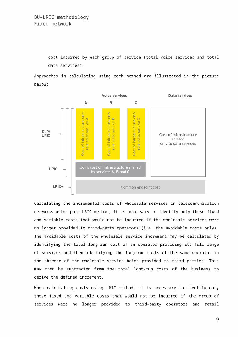
► Pure LRIC method – includes only costs related to network components used in the provision of the particular service (e.g. call termination).

► LRIC method – includes only costs related to network components used in the provision of the particular group of services, which allows some shared cost of the group of services to become incremental as well. The group of service could be defined as voice services or data services.

► LRIC+ method – includes costs described in LRIC+ method description plus common and joint cost. The common and joint cost related to each group of service (total voice services and total data services) are calculated separately for each Network Component using an equally-proportional mark-up (EPMU) mechanism based on the level of incremental cost incurred by each group of service (total voice services and total data services).

Approaches in calculating using each method are illustrated in the picture below:

7


Calculating the incremental costs of wholesale services in telecommunication networks using pure LRIC method, it is necessary to identify only those fixed and variable costs that would not be incurred if the wholesale services were no longer provided to third-party operators (i.e. the avoidable costs only). The avoidable costs of the wholesale service increment may be calculated by identifying the total long-run cost of an operator providing its full range of services and then identifying the long-run costs of the same operator in the absence of the wholesale service being provided to third parties. This may then be subtracted from the total long-run costs of the business to derive the defined increment.

When calculating costs using LRIC method, it is necessary to identify only those fixed and variable costs that would not be incurred if the group of services were no longer provided to third-party operators and retail subscribers (i.e. the avoidable costs only). The avoidable costs of the group of services increment may be calculated by identifying the total long-run cost of an operator providing its full range of services and then identifying the long-run costs of the same operator in the absence of the group of services being provided to third parties retail subscribers. This may then be subtracted from the total long-run costs of the business to derive the defined increment.

When calculating costs using LRIC+ additional mark-ups are added on the primarily estimated increments to cover costs of all shared and common elements and activities which are necessary for the provision of all services.

Cost of capital

8


The required return on investment in the network and other related assets are defined as the cost of capital. The cost of capital should allow the investors to get a return on network assets and other related assets on a same level as from comparable alternative investments. The cost of capital will be calculated taking into account the weighted average cost of capital (WACC) set by GNCC.

Scorched earth versus scorched node

One of the key decisions to be made with bottom-up modeling is whether to adopt a “scorched earth” or a “scorched node” assumption. The scorched earth approach assumes that optimally-sized network devices would be placed at locations optimal to the overall network design. It assumes that the network is redesigned on a greenfield site. The scorched earth approach assumes that optimally-sized network devices would be placed at the locations of the current nodes of operators.

Bottom-up

A bottom-up approach involves the development of engineering-economic models which are used to calculate the costs of network elements which would be used by an efficient operator in providing telecommunication services. Bottom-up models perform the following tasks:

Dimensioning and revaluation of the network.

Estimate network costs.

Estimate non-network costs.

Estimate operating maintenance and supporting costs.

Estimate services costs.

9


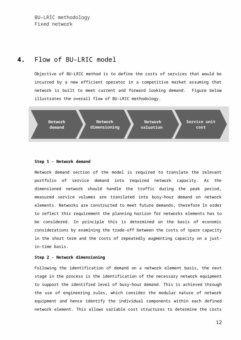
4. Flow of BU-LRIC modelObjective of BU-LRIC method is to define the costs of services that would be incurred by a new efficient operator in a competitive market assuming that network is built to meet current and forward looking demand. Figure below illustrates the overall flow of BU-LRIC methodology.

Step 1 - Network demand

Network demand section of the model is required to translate the relevant portfolio of service demand into required network capacity. As the dimensioned network should handle the traffic during the peak period, measured service volumes are translated into busy-hour demand on network elements. Networks are constructed to meet future demands, therefore In order to reflect this requirement the planning horizon for networks elements has to be considered. In principle this is determined on the basis of economic considerations by examining the trade-off between the costs of spare capacity in the short term and the costs of repeatedly augmenting capacity on a just-in-time basis.

Step 2 - Network dimensioning

Following the identification of demand on a network element basis, the next stage in the process is the identification of the necessary network equipment to support the identified level of busy-hour demand. This is achieved through the use of engineering rules, which consider the modular nature of network equipment and hence identify the individual components within each defined network element. This allows variable cost structures to determine the costs on an element-by-element basis.

Step 3 - Network valuation

After all the necessary network equipment it valuated and its cost are attributed to Homogenous Cost Categories (HCC) are derived. HCC is a set of costs, which have the same driver, the same cost volume relationship (CVR) pattern and the same rate of technology change. Network equipment identified during network dimensioning is

10

Network valuation

Service unit cost

Network dimensioni

ngNetwork demand


revalued at Gross Replacement Cost (GRC). The revaluation is done by multiplying the number of network equipment physical units by current prices of the equipment.

GRC is the basis to calculate the annual cost for each HCC which includes both:

► Annualized capital costs (CAPEX);► Annual operating expenses (OPEX).

CAPEX costs consist of cost of capital and depreciation. OPEX costs consist of salaries (including social insurance), material and costs of external services (outsourcing, transportation, security, utilities, etc).

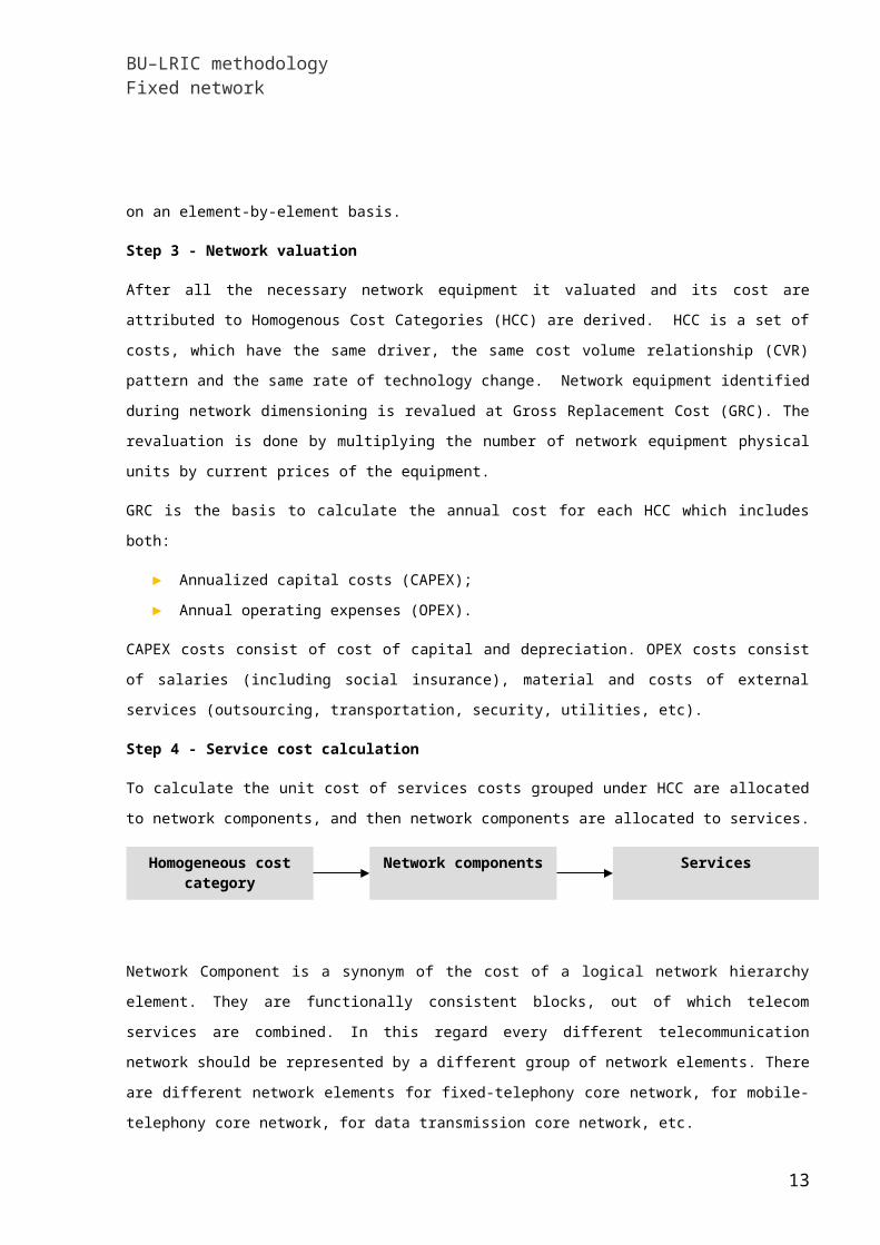
Step 4 - Service cost calculation

To calculate the unit cost of services costs grouped under HCC are allocated to network components, and then network components are allocated to services.

Network Component is a synonym of the cost of a logical network hierarchy element. They are functionally consistent blocks, out of which telecom services are combined. In this regard every different telecommunication network should be represented by a different group of network elements. There are different network elements for fixed-telephony core network, for mobile-telephony core network, for data transmission core network, etc.

All telecommunication networks represent a kind of hierarchy. Such network hierarchy consists of nodes (i.e.: in fixed-telephony core network nodes are switches) and paths between them (i.e.: transmission links in fixed-telephony core network). Such hierarchical view enables analysis of traffic flows going through specific logical network elements. Besides nodes and transmission links there is a number of supplementary network elements that represent service centers or other specialized devices (e.g. number portability, pre-selection etc.).

Due to the hierarchical structure of nodes and transmission links, different network components are defined for different hierarchical levels – either nodes or transmission links.

From the perspective of cost calculation of interconnection services only network elements representing fixed-telephony core network and mobile network are of interest. It means that all network elements representing other networks can be grouped together into one.

11

ServicesNetwork components

Homogeneous cost category


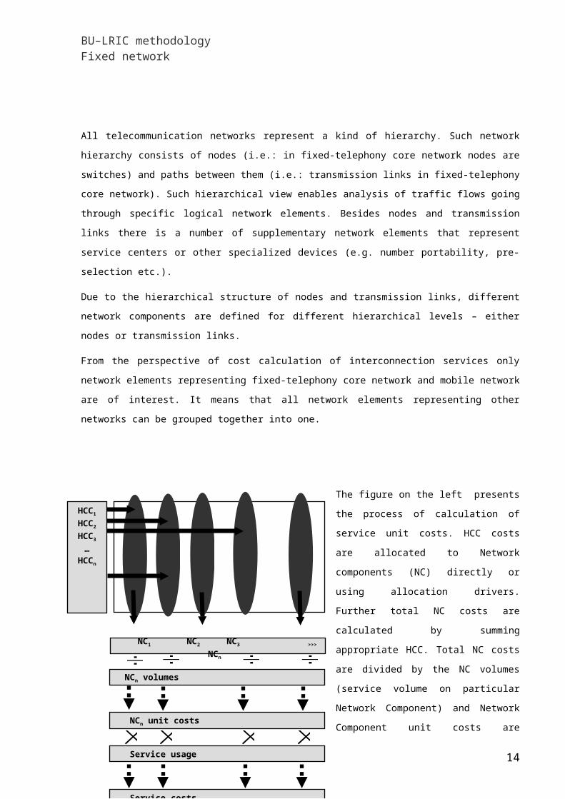
The figure on the left presents the process of calculation of service unit costs. HCC costs are allocated to Network components (NC) directly or using allocation drivers. Further total NC costs are calculated by summing appropriate HCC. Total NC costs are divided by the NC volumes (service volume on particular Network Component) and Network Component unit costs are calculated. Finally Network Component unit costs are multiplied by routing factor to calculate the service unit costs.

12

Service costs

Service usage

NCn unit costs

NCn volumes

NC1 NC2 NC3 >>>

HCC1HCC2HCC3

…HCCn


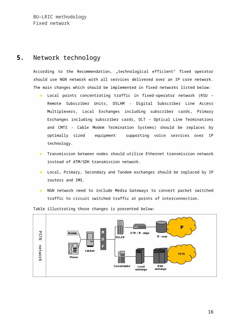
5. Network technologyAccording to the Recommendation, „technological efficient" fixed operator should use NGN network with all services delivered over an IP core network. The main changes which should be implemented in fixed networks listed below:

► Local points concentrating traffic in fixed-operator network (RSU – Remote Subscriber Units, DSLAM - Digital Subscriber Line Access Multiplexers, Local Exchanges including subscriber cards, Primary Exchanges including subscriber cards, OLT – Optical Line Terminations and CMTS - Cable Modem Termination Systems) should be replaces by optimally sized equipment supporting voice services over IP technology.

► Transmission between nodes should utilize Ethernet transmission network instead of ATM/SDH transmission network.

► Local, Primary, Secondary and Tandem exchanges should be replaced by IP routers and IMS.

► NGN network need to include Media Gateways to convert packet switched traffic to circuit switched traffic at points of interconnection.

Table illustrating those changes is presented below:

PSTN network architecture

MDF

IP

PSTNCabinet

ATM / IP - edgeDSLAM IP - core

Concentrator Local exchange

Inter exchange

Modem

Phone

13


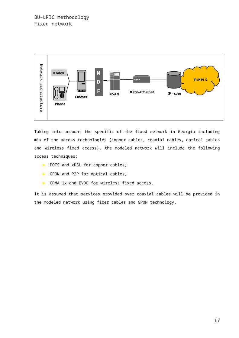
Network architecture according to EU

IP/MPLS

CabinetMetro-EthernetMSAN IP - core

MDF

Modem

Phone

Taking into account the specific of the fixed network in Georgia including mix of the access technologies (copper cables, coaxial cables, optical cables and wireless fixed access), the modeled network will include the following access techniques:

► POTS and xDSL for copper cables;► GPON and P2P for optical cables;► CDMA 1x and EVDO for wireless fixed access.

It is assumed that services provided over coaxial cables will be provided in the modeled network using fiber cables and GPON technology.

14


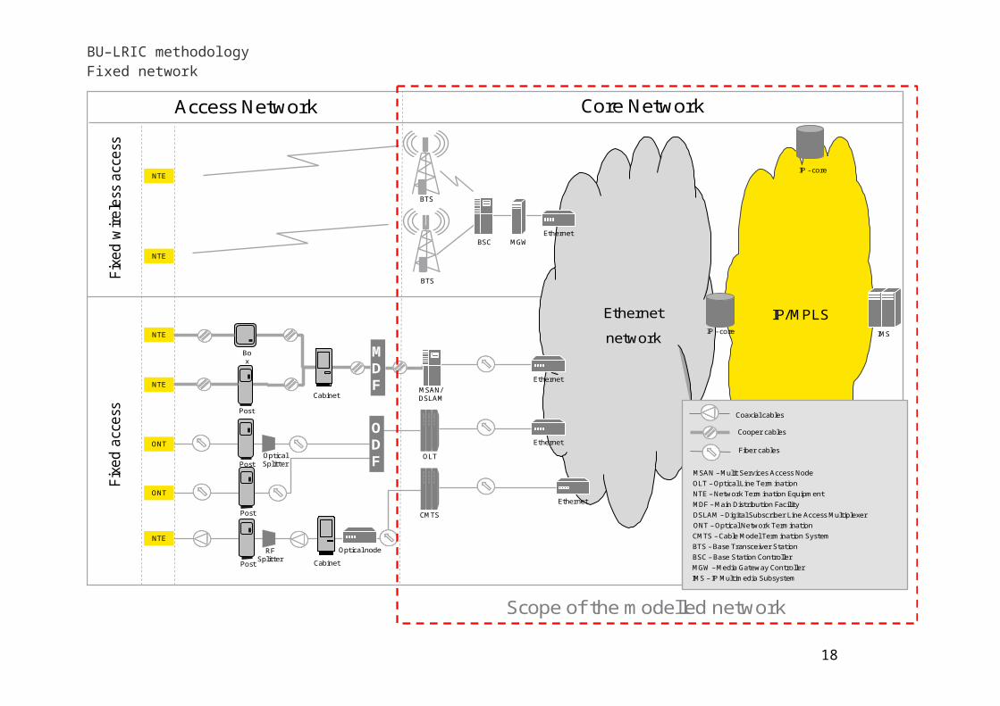
Ethernetnetwork

Ethernet

IP - core

MDF

Cabinet

Box

Post

NTE

NTE

ONT

MSAN/ DSLAM

NTE

OLT

ODF

CMTS

OpticalSplitterPost

RFSplitter Cabinet

Optical nodePost

MSAN – Mulit Services Access Node OLT – Optical Line TerminationNTE – Network Termination EquipmentMDF – Main Distribution FacilityDSLAM – Digital Subscriber Line Access Multiplexer

Cooper cables

Fiber cables

CMTS –Cable Model Termination System

Coaxial cables

ONT – Optical Network Termination

BSC

BTS

Ethernet

MGW

Ethernet

NTE

Ethernet

IP - core

IP/MPLS

NTE

ONT

Post

BTS

IMS

Access Network Core NetworkFix

ed w

ireles

s acc

ess

Fixed

acce

ss

BTS –Base Transceiver Station BSC – Base Station Controller MGW– Media Gateway Controller IMS – IP Multimedia Subsystem

Scope of the modelled network

15


6. Network structure and elements

6.1 Fixed network structure Core PSTN core switching network consist of separated switches and related equipment that ensures appearance and termination of temporary links among end points of the network. Switching network elements can be grouped into these categories:

► Remote Subscriber Unit (RSU)► Local Exchange;

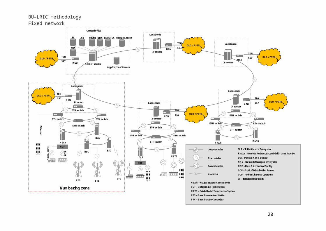
The local level of PSTN core network, which concentrates subscribes traffic, is formed by Remote Subscriber Units and Local Exchange. Geographical area which is usually served by one Local Exchange is called Numbering Zone.The main differences in PSTN and NGN network structure are:

► NGN network utilizes Multi Service Access Nodes to concentrate subscriber traffic, instead of Remote Subscriber Unit and Local Exchanges

► NGN network utilizes IP routers and IMS to transit and switch the traffic, instead of Exchanges.

The NGN network structure is presented on the schemas below.

16


Local node

Local node

Local node

IP router

OLO/ PSTNTDMSS7

ETH switch

IP router

ETH switch

ETH switch ETH switch

ODF

OLO/ PSTNTDMSS7

IMS

Central office

Billing NMS

OLO/ PSTN TDMSS7 IP router

OLO/ PSTNTDMSS7

ETH switch

ETH switch


MSANMSAN

OLO/ PSTNTDMSS7

ETH switch

IP router

ETH switch


MSANMDF

Ethernet

ISDN

PSTN/ xDSL

OLO/ PSTN TDMSS7

IN

DNS

MSAN– Mulit Services Access NodeOLT– Optical Line TerminationCMTS – Cable Model Termination SystemBTS – Base Transceiver Station BSC – Base Station Controller

Cooper cables

Fiber cables

IMS– IP Multimedia Subsystem Radius -Remote Authentication Dial In User ServiceDNS -Domain Name ServerNMS – Network Management SystemMDF – Main Distribution FacilityODF– Optical Distribution FrameOLO- Other Licensed Operator IN – Intelligent Network

HLR/HSS Radius Server

Applications Servers

Local node

Local node

MGW

MGW

MGW Core IP router

MGW

MGW

BSC

BTS BTSBTS

BSC

OLT CMTS

MGW

IP router MGW

Numbering zone

Coaxial cables

Radiolink

17

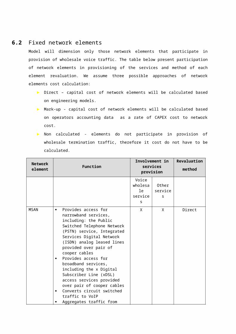
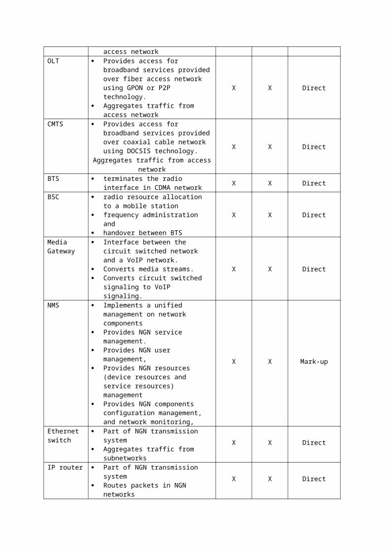
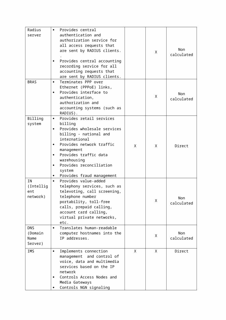
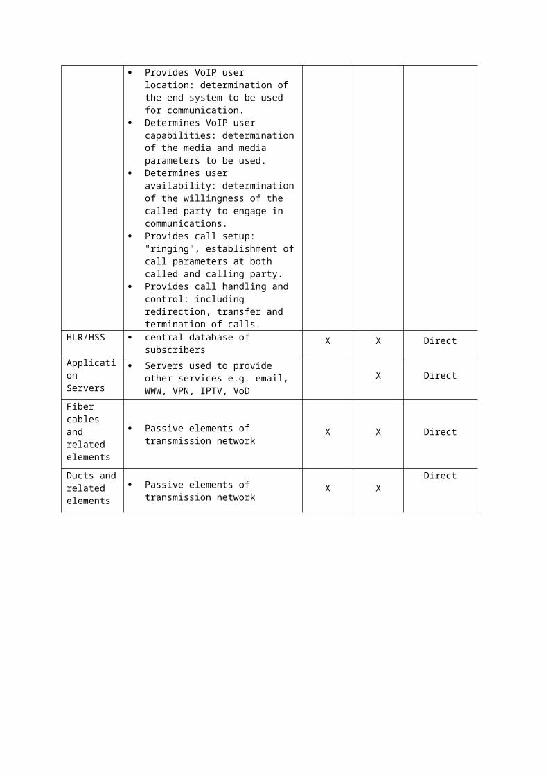
6.2 Fixed network elementsModel will dimension only those network elements that participate in provision of wholesale voice traffic. The table below present participation of network elements in provisioning of the services and method of each element revaluation. We assume three possible approaches of network elements cost calculation:

► Direct – capital cost of network elements will be calculated based on engineering models.

► Mark-up - capital cost of network elements will be calculated based on operators accounting data as a rate of CAPEX cost to network cost.

► Non calculated - elements do not participate in provision of wholesale termination traffic, therefore it cost do not have to be calculated.

Network element Function

Involvement in services provision

Revaluation method

Voice wholesal

e services

Other services

MSAN Provides access for narrowband services, including: the Public Switched Telephone Network (PSTN) service, Integrated Services Digital Network (ISDN) analog leased lines provided over pair of cooper cables

Provides access for broadband services, including the x Digital Subscriber Line (xDSL) access services provided over pair of cooper cables

Converts circuit switched traffic to VoIP

Aggregates traffic from access network

X X Direct

OLT Provides access for broadband services provided over fiber access network using GPON or P2P technology.

Aggregates traffic from access network

X X Direct

CMTS Provides access for broadband services provided over coaxial cable network using DOCSIS technology.Aggregates traffic from access

network

X X Direct

BTS terminates the radio interface in CDMA network X X Direct

BSC radio resource allocation to a X X Direct

mobile station frequency administration and handover between BTS

Media Gateway

Interface between the circuit switched network and a VoIP network.

Converts media streams. Converts circuit switched

signaling to VoIP signaling.

X X Direct

NMS Implements a unified management on network components

Provides NGN service management.

Provides NGN user management,

Provides NGN resources (device resources and service resources) management

Provides NGN components configuration management, and network monitoring,

X X Mark-up

Ethernet switch

Part of NGN transmission system Aggregates traffic from

subnetworksX X Direct

IP router Part of NGN transmission system Routes packets in NGN networks

X X DirectRadius server

Provides central authentication and authorization service for all access requests that are sent by RADIUS clients. .

Provides central accounting recording service for all accounting requests that are sent by RADIUS clients.

X Non calculated

BRAS Terminates PPP over Ethernet (PPPoE) links,

Provides interface to authentication, authorization and accounting systems (such as RADIUS).

X Non calculated

Billing system

Provides retail services billing Provides wholesale services

billing - national and international

Provides network traffic management

Provides traffic data warehousing

Provides reconciliation system Provides fraud management

X X Direct

IN (Intelligent network)

Provides value-added telephony services, such as televoting, call screening, telephone number portability, toll-free calls, prepaid calling, account card calling, virtual private networks, etc.

X Non calculated

DNS (Domain Name Server)

Translates human-readable computer hostnames into the IP addresses. X Non

calculated

IMS Implements connection management and control of voice, data and multimedia services based on the IP network

Controls Access Nodes and Media Gateways

Controls NGN signaling Provides VoIP user location:

determination of the end system to be used for communication.

Determines VoIP user capabilities: determination of the media and media parameters to be used.

Determines user availability: determination of the willingness of the called party to engage in communications.

Provides call setup: "ringing", establishment of call parameters at both called and calling party.

Provides call handling and control: including redirection, transfer and termination of calls.

X X Direct

HLR/HSS central database of subscribers X X DirectApplication Servers

Servers used to provide other services e.g. email, WWW, VPN, IPTV, VoD

X Direct

Fiber cables and related elements

Passive elements of transmission network

X X Direct

Ducts and related elements

Passive elements of transmission network

X XDirect

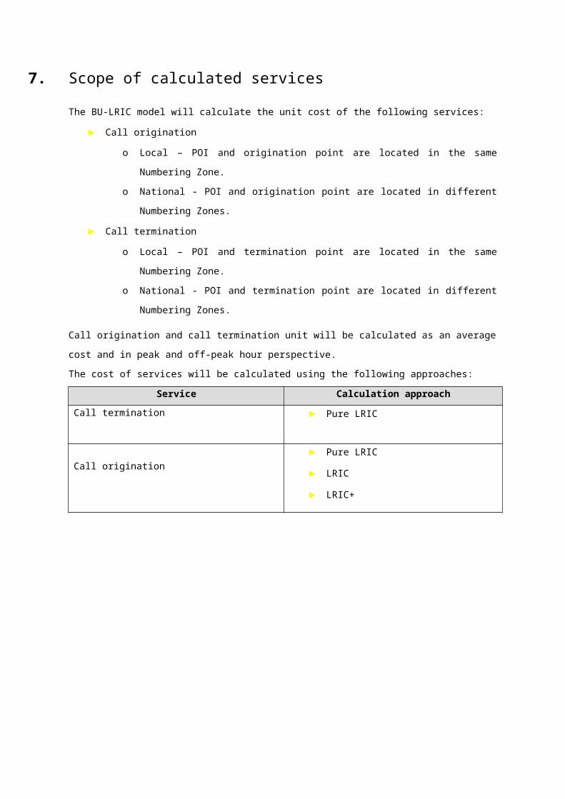
7. Scope of calculated servicesThe BU-LRIC model will calculate the unit cost of the following services:

► Call originationo Local – POI and origination point are located in the same Numbering Zone.o National - POI and origination point are located in different Numbering

Zones.► Call termination

o Local – POI and termination point are located in the same Numbering Zone.

o National - POI and termination point are located in different Numbering Zones.

Call origination and call termination unit will be calculated as an average cost and in peak and off-peak hour perspective.The cost of services will be calculated using the following approaches:

Service Calculation approachCall termination ► Pure LRIC

Call origination► Pure LRIC► LRIC► LRIC+

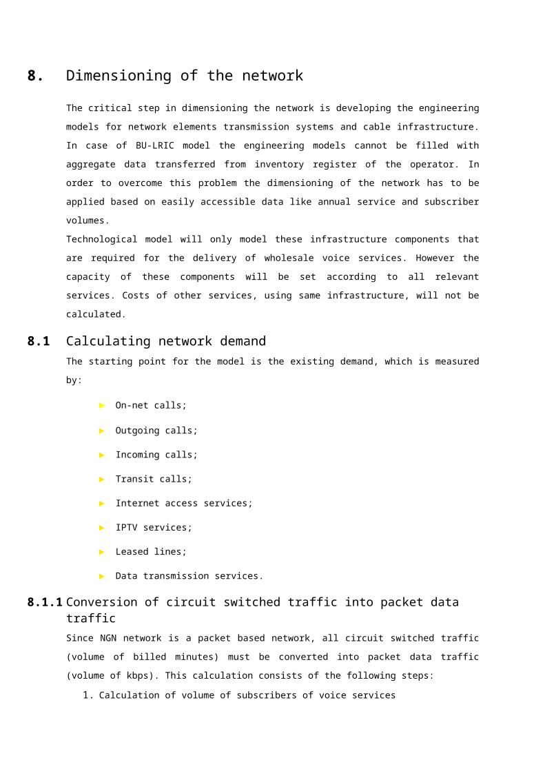
8. Dimensioning of the network The critical step in dimensioning the network is developing the engineering models for network elements transmission systems and cable infrastructure. In case of BU-LRIC model the engineering models cannot be filled with aggregate data transferred from inventory register of the operator. In order to overcome this problem the dimensioning of the network has to be applied based on easily accessible data like annual service and subscriber volumes.Technological model will only model these infrastructure components that are required for the delivery of wholesale voice services. However the capacity of these components will be set according to all relevant services. Costs of other services, using same infrastructure, will not be calculated.

8.1 Calculating network demandThe starting point for the model is the existing demand, which is measured by:

► On-net calls;

► Outgoing calls;

► Incoming calls;

► Transit calls;

► Internet access services;

► IPTV services;

► Leased lines;

► Data transmission services.

8.1.1 Conversion of circuit switched traffic into packet data trafficSince NGN network is a packet based network, all circuit switched traffic (volume of billed minutes) must be converted into packet data traffic (volume of kbps). This calculation consists of the following steps:

1. Calculation of volume of subscribers of voice services

Based on the engineering model of Access Nodes (MSAN, OLT, BTS), the number of subscribers of voice services will be calculated.

2. Calculation of BHT (Busy Hour Traffic) per subscriber

Based on busy hour traffic demand on Access Nodes and the volume of subscribers of voice services from the first step, the volume of BHmE (Busy Hour mili Erlangs) per subscriber will be calculated.

3. Calculation of volume of BHE (Busy Hour Erlangs) for each Access Node

For each Access Node the volume of BHE will be calculated. This will be done by multiplying the volume subscribers of voice services by volume of BHmE (Busy Hour mili Erlangs) per subscriber. The volume of BHE determines how many VoIP channels are required to handle the voice traffic in the busy hour.

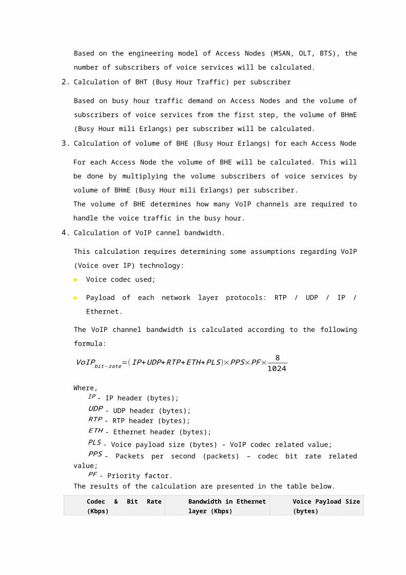
4. Calculation of VoIP cannel bandwidth.

This calculation requires determining some assumptions regarding VoIP (Voice over IP) technology:► Voice codec used;

► Payload of each network layer protocols: RTP / UDP / IP / Ethernet.

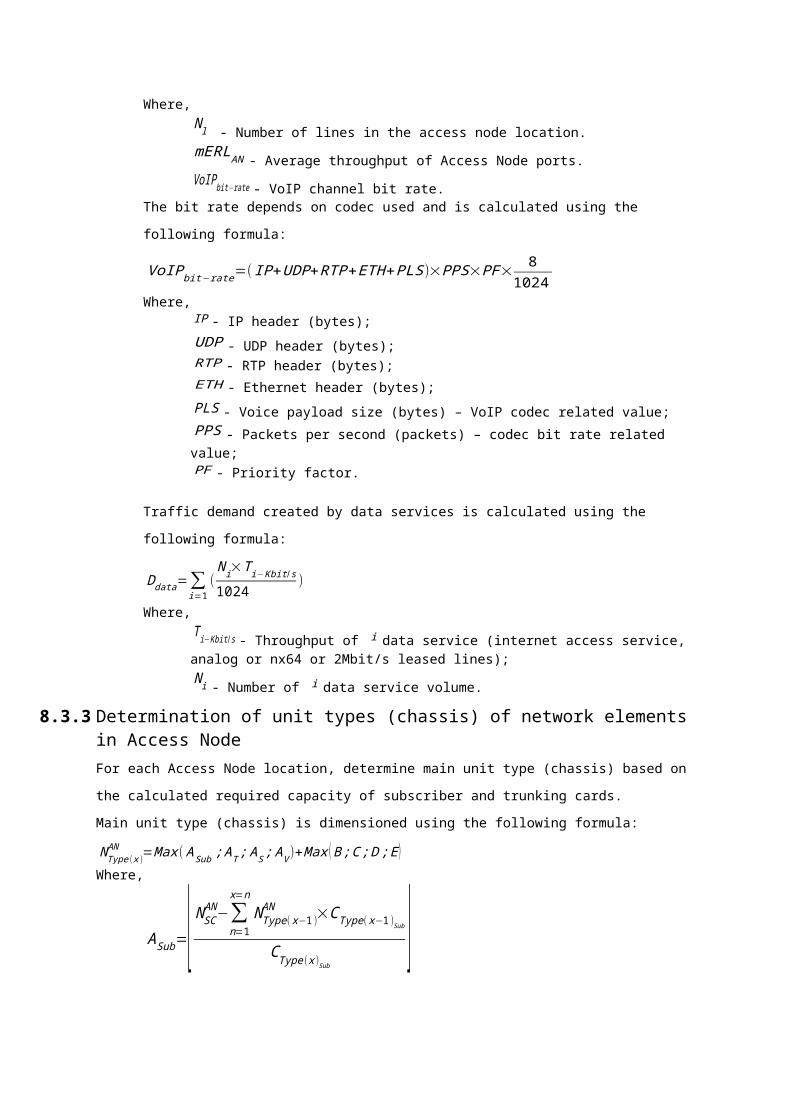
The VoIP channel bandwidth is calculated according to the following formula:

VoIPbit−rate=( IP+UDP+RTP+ETH+PLS )×PPS×PF× 81024

Where,IP - IP header (bytes);UDP - UDP header (bytes);RTP - RTP header (bytes);ETH - Ethernet header (bytes);PLS - Voice payload size (bytes) – VoIP codec related value;PPS - Packets per second (packets) – codec bit rate related value;PF - Priority factor.

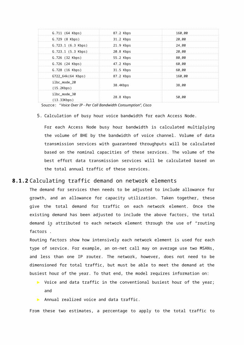
The results of the calculation are presented in the table below.Codec & Bit Rate (Kbps)

Bandwidth in Ethernet layer (Kbps)

Voice Payload Size (bytes)

G.711 (64 Kbps) 87.2 Kbps 160,00G.729 (8 Kbps) 31.2 Kbps 20,00G.723.1 (6.3 Kbps) 21.9 Kbps 24,00G.723.1 (5.3 Kbps) 20.8 Kbps 20,00G.726 (32 Kbps) 55.2 Kbps 80,00G.726 (24 Kbps) 47.2 Kbps 60,00G.728 (16 Kbps) 31.5 Kbps 60,00G722_64k(64 Kbps) 87.2 Kbps 160,00ilbc_mode_20 (15.2Kbps) 38.4Kbps 38,00ilbc_mode_30 (13.33Kbps) 28.8 Kbps 50,00

Source: “Voice Over IP - Per Call Bandwidth Consumption”, Cisco

5. Calculation of busy hour voice bandwidth for each Access Node.

For each Access Node busy hour bandwidth is calculated multiplying the volume of BHE by the bandwidth of voice channel. Volume of data transmission services with guaranteed throughputs will be calculated based on the nominal capacities of these services. The volume of the best effort data transmission services will be

calculated based on the total annual traffic of these services.

8.1.2 Calculating traffic demand on network elementsThe demand for services then needs to be adjusted to include allowance for growth, and an allowance for capacity utilization. Taken together, these give the total demand for traffic on each network element. Once the existing demand has been adjusted to include the above factors, the total demand is attributed to each network element through the use of “routing factors”.Routing factors show how intensively each network element is used for each type of service. For example, an on-net call may on average use two MSANs, and less than one IP router. The network, however, does not need to be dimensioned for total traffic, but must be able to meet the demand at the busiest hour of the year. To that end, the model requires information on:

► Voice and data traffic in the conventional busiest hour of the year; and► Annual realized voice and data traffic.

From these two estimates, a percentage to apply to the total traffic to estimate the dimensioned busy hour can be derived.

8.2 Active network equipment dimensioning approach 8.2.1 Base and extension units concept

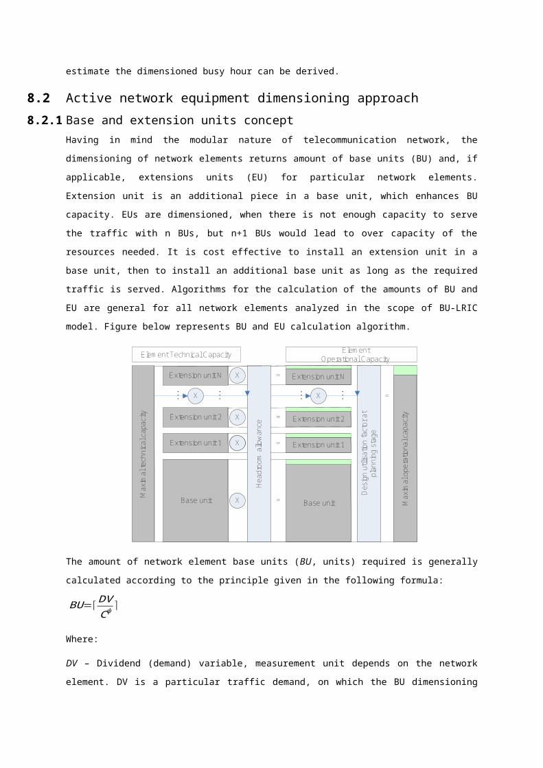
Having in mind the modular nature of telecommunication network, the dimensioning of network elements returns amount of base units (BU) and, if applicable, extensions units (EU) for particular network elements. Extension unit is an additional piece in a base unit, which enhances BU capacity. EUs are dimensioned, when there is not enough capacity to serve the traffic with n BUs, but n+1 BUs would lead to over capacity of the resources needed. It is cost effective to install an extension unit in a base unit, then to install an additional base unit as long as the required traffic is served. Algorithms for the calculation of the amounts of BU and EU are general for all network elements analyzed in the scope of BU-LRIC model. Figure below represents BU and EU calculation algorithm.

Base unit

Extension unit 1

Extension unit 2

Extension unit N

...

ElementOperational CapacityElement Technical Capacity

Extension unit 1

Extension unit 2

Extension unit N

...

Max

imal

tech

nica

l cap

acity

Base unit

=

=

=

= Max

imal

ope

ratio

nal c

apac

ity

Des

ign

utili

satio

n fa

ctor

at

plan

ning

sta

ge

Hea

droo

m a

llow

ance

X

X

XX

X

X ... ... X =

The amount of network element base units (BU, units) required is generally calculated according to the principle given in the following formula:

BU=⌈ DVCψ

⌉

Where:

DV – Dividend (demand) variable, measurement unit depends on the network element. DV is a particular traffic demand, on which the BU dimensioning depends directly.

Cψ – Maximal operational capacity of network element, measurement unit is the same as for DV.

Operational capacity of a base unit or extension unit shows what traffic volumes it can maintain.

The amount of network element extension units (EU, units) required, if applicable, is generally calculated according to the principle given in the following formula:

EU=⌈BU×(Cψ−CBU

ο )CES

ο ⌉

Where:

Cψ – Maximal operational capacity of a network element, measurement unit is the same as for DV.

BU – Base unit, units;

CBUο

– Base unit operational capacity, measurement unit depends on the network element;

CESο

– Extension step (additional extension unit to BU) operational capacity,

measurement unit depends on the network element.

Maximal operational capacity (Cψ, BHCA, subscribers, etc.) for a particular network element is calculated according to the principle given in the following formula:

Cψ=C τ×OA

BU and EU operational capacity (C iο, BHCA, subscribers, etc.) are calculated according to

the principle given in the following formula by applying capacity values respectively.C i

ο=Ci×OAi

Where:

C τ – Maximal technical capacity (including possible extension), measurement unit

depends on the element. Cτshows maximal technical theoretical capacity of a network

element in composition of BU and EU.

Ci – Base unit or extension unit capacity, measurement unit depends on the element. Ci

defines technical parameter of BU or EU capacity.

i – Specifies BU or EU.

OA – Operational allowance, %.

Operational allowance (OA, %) shows both design and future planning utilization of a network equipment, expressed in percents. OA is calculated according to the principle given in the following formula:OA=HA× f U

Where:

HA – Headroom allowance, %. HA shows what part of BU or EU capacity is reserved for future traffic growth.

fU – Design utilization factor at a planning stage, %. It is equipment (vendor designated) maximum utilization parameter. This utilization parameter ensures that the equipment in the network is not overloaded by any transient spikes in demand as well as represents the redundancy factor. Operational allowance and capacity calculations depend on the headroom allowance figure (HA, %). Headroom allowance is calculated according to the principle given in the following formula:

HA= 1r SDG

Where:

rSDG – Service demand growth ratio.

rSDG determines the level of under-utilization in the network, as a function of equipment planning periods and expected demand. Planning period shows the time it takes to make all the necessary preparations to bring new equipment online. This period can be from weeks to years. Consequently, traffic volumes by groups (demand aggregates given below) are planned according to the service demand growth.

The service demand growth ratio is calculated for each one of the following demand aggregates:

► Total subscribers number;

► CCS traffic, which comprises of voice, circuit data and converted to minute equivalent video traffic;

► Air interface traffic, which comprises of converted to minute equivalent SMS, MMS and packet data traffic. Packet data traffic in this case means GSM, UMTS and LTE traffic sum of up-link or down-link traffic subject to greater value.

A particular demand growth ratio is assigned to a particular network element’s equipment.

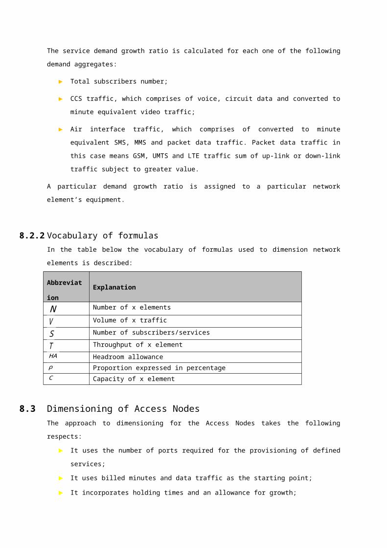
8.2.2 Vocabulary of formulasIn the table below the vocabulary of formulas used to dimension network elements is described:

Abbreviation

Explanation

N Number of x elements

V Volume of x traffic

S Number of subscribers/services

T Throughput of x elementHA Headroom allowanceρ Proportion expressed in percentageC Capacity of x element

8.3 Dimensioning of Access NodesThe approach to dimensioning for the Access Nodes takes the following respects:

► It uses the number of ports required for the provisioning of defined services;► It uses billed minutes and data traffic as the starting point;► It incorporates holding times and an allowance for growth;

► It uses routing factors to determine the intensity with which each network element is used;

► It dimensions the network to meet the busy hour demand; ► It then adjusts this capacity to allow for flows between nodes and to provide

resilience.

Dimensioning of the Access Nodes will be performed according to the scorched node approach. Scorched earth approach is not used in dimensioning Access Network in order not to affect the market of wholesale access services currently provided at access node locations. Assumptions of Scorched Node approach are as follows:

► For each Access Node location collect geographical data (address, coordinates) – scorched node approach, which will not affect wholesale access services;

► For each Access Node location collect volume of connected services. Specifically: o voice services provided over cooper access network, optical access

network, coaxial access network, wireless access network, ISDN BRA services, ISDN PRA services.

o Internet access services provided over cooper access network, optical access network using GPON or P2P architecture, coaxial access network and wireless access network.

o TDM leased lines, ATM/Ethernet data transmission services.► It is assumed that leased lines will be provided based on SDSL/HDSL technology;► It is assumed that high speed TDM leased lines will be provided based on Ethernet

technology;► ATM data transmission services will be provided based on Ethernet technology;► MSANs will be dimensioned where support of subscribers connected to the

network over POTS, ISDN and xDSL technologies is necessary;► Access Ethernet Switches will be dimensioned where support of subscribers

connected to the network over Point to Point technology is necessary;► Optical Line Terminals will be dimensioned where support of subscribers

connected to the network over GPON or coaxial cables technology is necessary.► CDMA base stations will be dimensioned where support of subscribers connected

to the network over CDMA technology is necessary.

After the information is collected and the stated assumption takes place, dimensioning the number of required equipment in Access Nodes is calculated in these steps:

1) Calculation of the average throughput per port utilized by subscribers of voice services and the average throughput per port utilized by the subscribers of data services for each network component;

2) Calculation of number of subscriber and trunking ports needed at each Access Node location, using the calculated throughputs to estimate the demand of traffic through the mentioned ports;

3) Determination of network element’s main unit type (chassis) for each Access Node location depending on the number of subscriber and trunking cards needed at each Access Node location;

8.3.1 Calculation of average throughput of Access Node network elementsAverage throughput per ports utilized by the subscribers of voice services based on network demand calculation is calculated using the following formula:

mERLNC=V r⋅rBHT / AVG⋅RFNC

N l+NGPON /P2P⋅1000365⋅24⋅60

Where,mERLNC - Average throughput per port for each network component (NC);V r - Total realized services volume;rBHT / AVG - Busy Hour to Average Hour traffic ratio. This factor shows the proportion of busy and average traffic;RFNC - Average utilization of network component.N l - Volume of equivalent voice linesNGPON /P2P - Number of GPON and Point to Point voice subscribers.

The volume of equivalent voice lines is calculated using the following formula:N l=mPOTS×N POTS+mIBRA×N BRA+mIPRA×N PRA

Where,N l - Number of equivalent voice lines;N POTS - Number of voice lines;N BRA - Number of ISDN-BRA lines;N PRA - Number of ISDN-PRA lines;mPOTS=1 - Equivalent voice channels – POTS;mBRA=2 - Equivalent voice channels - ISDN-BRA;mPRA=30 - Equivalent voice channels - ISDN-PRA.

The average utilization of network component is calculated using the following formula:

RFNC=

V tw

V r

Where,V tw - Total weighted voice service volume on network component;V r - Total realized voice service volume;RFNC - Average utilization of network component.

The total weighted service volumes for each network component are calculated using the following formula:

V tw=∑i

n

V i×RFi

Where,V tw - Total weighted voice services volume on network component;

V i- Service volume of i -voice service;

RF - Routing factor of i voice service defined for particular network component.i - Voice service;n - Number of voice services.

The average throughput per ports utilized by subscribers of data services based on average throughputs and overbooking factors is calculated using the following formula:

T X−Kbit/ s=V x×PF x

S x⋅10242

Where,T X−Kbit/ s - Average data throughput per port;V x - Data service Busy Hour traffic;Sx - Total amount ofx services;PF x - Priority factor forx service;

8.3.2 Calculation of number of ports in Access NodesFor each Access Node location the number of services y (POTS, xDSL, GPON, P2P, coaxial) is calculated using the following formula:

NY −ports=

V ly×S y

V y

Where,NY −ports - Number ofy services;V ly - Volume of y services at l access node location;S y - Total amount of y users/subscribers;

V y - Total amount of y services provided at access nodes.

For each Access Node location the calculation of trunking ports (GE, 10 GE) based on the required capacity and technical assumptions (ring structure, redundancy) is done using the following formulas:For OLT and Access Ethernet Switches:

N t− ports=⌈D voice−fiber+Ddata−fiber+DIPTV

1024×HA⌉×2

Where,Dvoice− fiber - Demand from voice services provided over fiber in Mbit/s. It is calculated by multiplying the traffic generated by voice services in Erlangs provided over GPON, P2P and DOCSIS technologies in Access

Node location by VoIPbit−rate VoIP channel bit rate;Ddata−fiber - Demand from data services provided over fiber in Mbit/s. HA - Headroom allowance;D IPTV - Demand from IPTV services provided over fiber in Mbit/s.

Demand from IPTV services is calculated using the following formula:

D IPTV=N IPTV−ports×T VOD−Kbit / s+min ( N IPTV −ports×T IPTV−Kbit /s ; N channels×Tchannel )Where,

N IPTV− ports - Number of IPTV services present at Access Node location;T IPTV−Kbit /s - Average throughput of IPTV service; T VOD−Kbit /s - Average throughput of VOD service;Nchannels - Maximal amount of channels provided to the subscribers;T channel - Average throughput required to show one channel via IPTV.

For MSAN:

N MSAN−t−ports=⌈Dvoice+Ddata

1024×HA⌉×2

Where,N MSAN−t−ports - Number of trunking ports;HA - Headroom allowance;Dvoice - Demand from voice services in Mbit/s;Ddata - Demand from data services in Mbit/s;

Traffic demand created by voice services is calculated using the following formula:

Dvoice=N l×mERLAN×VoIPbit−rate×1

1000×1024Where,

N l - Number of lines in the access node location.mERLAN - Average throughput of Access Node ports. VoIPbit−rate - VoIP channel bit rate.

The bit rate depends on codec used and is calculated using the following formula:

VoIPbit−rate=( IP+UDP+RTP+ETH+PLS )×PPS×PF× 81024

Where,IP - IP header (bytes);UDP - UDP header (bytes);RTP - RTP header (bytes);ETH - Ethernet header (bytes);PLS - Voice payload size (bytes) – VoIP codec related value;PPS - Packets per second (packets) – codec bit rate related value;PF - Priority factor.

Traffic demand created by data services is calculated using the following formula:

Ddata=∑i=1

(N i×T i−Kbit /s

1024)

Where,T i−Kbit / s - Throughput of i data service (internet access service, analog or nx64 or 2Mbit/s leased lines);N i - Number of i data service volume.

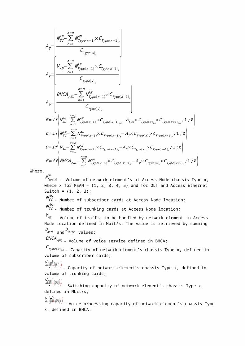
8.3.3 Determination of unit types (chassis) of network elements in Access NodeFor each Access Node location, determine main unit type (chassis) based on the calculated required capacity of subscriber and trunking cards. Main unit type (chassis) is dimensioned using the following formula:NType ( x )

AN =Max ( A Sub ; AT ; AS ; AV )+Max ( B ;C ; D; E )Where,

ASub=⌊ N SCAN−∑

n=1

x=n

NType ( x−1 )AN ×CType (x−1)Sub

CType ( x )Sub

⌋AT=⌊ N TC

AN−∑n=1

x=n

N Type( x−1)AN ×CType ( x−1)T

CType ( x )T⌋

AS=⌊ V AN−∑n=1

x=n

N Type( x−1)AN ×CType ( x−1)S

CType (x )S

⌋AV =⌊ BHCA ANL−∑

n=1

x=n

NType ( x−1)AN ×CType (x−1)V

CType ( x )V⌋

B=if (N SCAN−∑

n=1

x=n

NType (x−1 )AN ×CType (x−1)Sub

−ASub×CType (x )Sub>CType (x+1)Sub

;1;0)C=if (NTC

AN−∑n=1

x=n

N Type (x−1)AN ×CType( x−1)T

−AT×CType ( x )T>CType (x+1 )T

;1; 0)D=if (V AN−∑

n=1

x=n

NType (x−1 )AN ×CType (x−1 )S

−A S×CType (x )S>CType (x+1)S

;1 ;0)E=if (BHCA ANL−∑

n=1

x=n

NType ( x−1)AN ×CType (x−1 )V

−AV×CType( x )V>CType ( x+1 )V

;1 ;0)Where,

NType (x )AN

- Volume of network element’s at Access Node chassis Type x, where x for MSAN = {1, 2, 3, 4, 5} and for OLT and Access Ethernet Switch = {1, 2, 3}; N SC

AN- Number of subscriber cards at Access Node location;

NTCAN

- Number of trunking cards at Access Node location;V AN - Volume of traffic to be handled by network element in Access Node location defined in Mbit/s. The value is retrieved by summing Ddata andDvoice values;BHCAANL - Volume of voice service defined in BHCA;CType( x )Sub - Capacity of network element’s chassis Type x, defined in volume of subscriber cards;

Calignl ¿ Type (x )T ¿¿¿- Capacity of network element’s chassis Type x, defined in volume of trunking cards;

Calignl ¿Type ( x )S ¿ ¿¿- Switching capacity of network element’s chassis Type x, defined in Mbit/s;

Calignl ¿ Type (x )V ¿¿¿- Voice processing capacity of network element’s chassis Type x, defined in BHCA.

For OLT and Access Ethernet Switches, the main unit types are estimated without

including the AS ; AV ; D ; Eparts of the formula.

Calculation of the required subscriber cards per Access Node location is done using the following formulas:

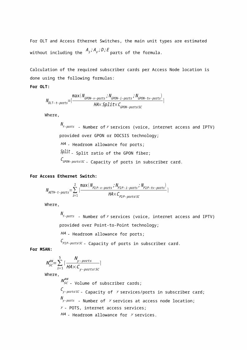
For OLT:

NOLT −t−ports=⌈max(N GPON−v− ports ; NGPON−i−ports ; NGPON−tv−ports )

HA×Split×CGPON−ports /SC⌉

Where,NY −ports - Number ofy services (voice, internet access and IPTV) provided over GPON or DOCSIS technology;HA - Headroom allowance for ports;Split - Split ratio of the GPON fiber;CGPON− ports /SC - Capacity of ports in subscriber card.

For Access Ethernet Switch:

N AETH−t− ports=∑i=1

2

⌈max( NP2P−v−ports ;N P2P−i−ports ; N P2P−tv− ports)

HA×C P2P− ports /SC⌉

Where,NY −ports - Number ofy services (voice, internet access and IPTV) provided over Point-to-Point technology;HA - Headroom allowance for ports;CP2P−ports /SC - Capacity of ports in subscriber card.

For MSAN:

N SCAN=∑

i=1

5

⌈N y−ports

HA×C y−ports /SC⌉

Where,N SC

AN- Volume of subscriber cards;

C y−ports / SC - Capacity of y services/ports in subscriber card;N y−ports - Number of y services at access node location;y - POTS, internet access services;HA - Headroom allowance for y services.

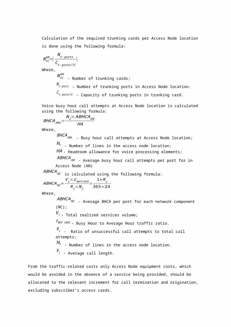
Calculation of the required trunking cards per Access Node location is done using the following formula:

NTCAN=⌈

N t−ports

C t−ports/TC⌉

Where,NTC

AN - Number of trunking cards;

N t−ports - Number of trunking ports in Access Node location.C t−ports/TC - Capacity of trunking ports in trunking card.

Voice busy hour call attempts at Access Node location is calculated using the following formula:

BHCAANL=N l×ABHCA AN

HAWhere,

BHCAANL - Busy hour call attempts at Access Node location;lN - Number of lines in the access node location;

HA - Headroom allowance for voice processing elements;ABHCAAN - Average busy hour call attempts per port for in Access Node (AN)

ABHCANC is calculated using the following formula:

ABHCANC=V r×rBHT / AVG

Rl×N l×1+Rr

365×24Where,

ABHCANC - Average BHCA per port for each network component (NC);rV - Total realized services volume;

AVGBHTr / - Busy Hour to Average Hour traffic ratio.Rr - Ratio of unsuccessful call attempts to total call attempts;

lN - Number of lines in the access node location. Rl - Average call length.

From the traffic-related costs only Access Node equipment costs, which would be avoided in the absence of a service being provided, should be allocated to the relevant increment for call termination and origination, excluding subscriber’s access cards.

8.4 Dimensioning the Radio Access Network8.4.1 Base Stations dimensioning

CDMA macrocell range and sector capacity are calculated separately for different area types. In CDMA system the cell range is dependent on current traffic, the footprint of CDMA cell is dynamically expanding and contradicts according to the number of users. This feature of CDMA is called “cell breathing”. Implemented algorithm calculates optimal CDMA cell range with regard to the cell required capacity (demand). This calculation is performed in four steps:

1) Required CDMA network capacity by cell types

In this step the required CDMA network capacity for uplink and downlink channel is calculated based on voice and data traffic demand. The CDMA network capacity is calculated separately for different area type.

2) Traffic BH density per 1km2

In this step traffic BH density per 1km2 is calculated based on the required CDMA network capacity and required coverage of CDMA network. The CDMA traffic BH density per 1 km2

is calculated separately for uplink and downlink channel for each area type.

3) Downlink and uplink calculation

In this section implemented algorithm finds the relationship (function) between cell area and cell capacity, separately for uplink and downlink channel and different area type. To find relationship (function) formula algorithm uses two function extremes:

1) x: Maximal cell range assuming minimal capacity consumptiony: Minimal site capacity volume (single data channel)

2) x: Maximal cell range assuming full capacity consumptiony: Maximal site capacity volume

Then according to traffic BH density per 1 km2 and found relationship (function) formula, the optimal cell area and sector capacity is calculated separately for different area type.

4) Total

In this last step the optimal CDMA macrocell range and sector capacity is calculated separately for uplink and downlink channel and different area type.

The values presenting:

1) x: Maximal cell range assuming minimal capacity consumptiony: Minimal site capacity volume (single data channel)

2) x: Maximal cell range assuming full capacity consumptiony: Maximal site capacity volume

will be gathered from operators and verified based on link budget calculation.

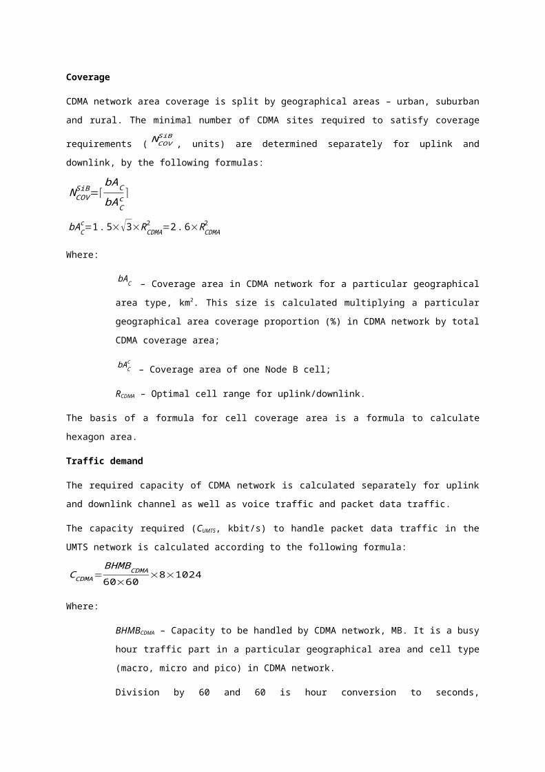
Coverage

CDMA network area coverage is split by geographical areas – urban, suburban and rural.

The minimal number of CDMA sites required to satisfy coverage requirements (NCOVSiB

, units) are determined separately for uplink and downlink, by the following formulas:

NCOVSiB =⌈

bAC

bACc ⌉

bACc =1. 5×√3×RCDMA

2 =2 .6×RCDMA2

Where:

bAC – Coverage area in CDMA network for a particular geographical area type, km2. This size is calculated multiplying a particular geographical area coverage proportion (%) in CDMA network by total CDMA coverage area;

bACc

– Coverage area of one Node B cell;

RCDMA – Optimal cell range for uplink/downlink.

The basis of a formula for cell coverage area is a formula to calculate hexagon area.

Traffic demand

The required capacity of CDMA network is calculated separately for uplink and downlink channel as well as voice traffic and packet data traffic.

The capacity required (CUMTS, kbit/s) to handle packet data traffic in the UMTS network is calculated according to the following formula:

CCDMA=BHMBCDMA

60×60×8×1024

Where:

BHMBCDMA – Capacity to be handled by CDMA network, MB. It is a busy hour traffic part in a particular geographical area and cell type (macro, micro and pico) in CDMA network.

Division by 60 and 60 is hour conversion to seconds, multiplication by 8 is a bytes conversion to bits and multiplication by 1024 is megabyte conversion to kilobytes.

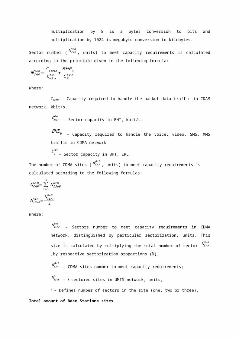
Sector number (NCAPSeB

, units) to meet capacity requirements is calculated according to the principle given in the following formula:

NCAPSeB =

CCDMA

CminSe +

BHEV

CVErl

Where:

CCDMA – Capacity required to handle the packet data traffic in CDAM network, kbit/s.

CminSe

– Sector capacity in BHT, kbit/s.

BHEV – Capacity required to handle the voice, video, SMS, MMS traffic in CDMA network

CVErl

- Sector capacity in BHT, ERL.

The number of CDMA sites (NCAPSiB

, units) to meet capacity requirements is calculated according to the following formulas:

NCAPSiB =∑

i=1

3

N iSeBSiB

N iSeBSiB =

N iCAPSeB

i

Where:

N iCAPSeB

– Sectors number to meet capacity requirements in CDMA network, distinguished by particular sectorization, units. This size is calculated by

multiplying the total number of sector NCAPSeB

,by respective sectorization proportions (%);

NCAPSiB

– CDMA sites number to meet capacity requirements;

N iSeBSi

– i sectored sites in UMTS network, units;

i – Defines number of sectors in the site (one, two or three).

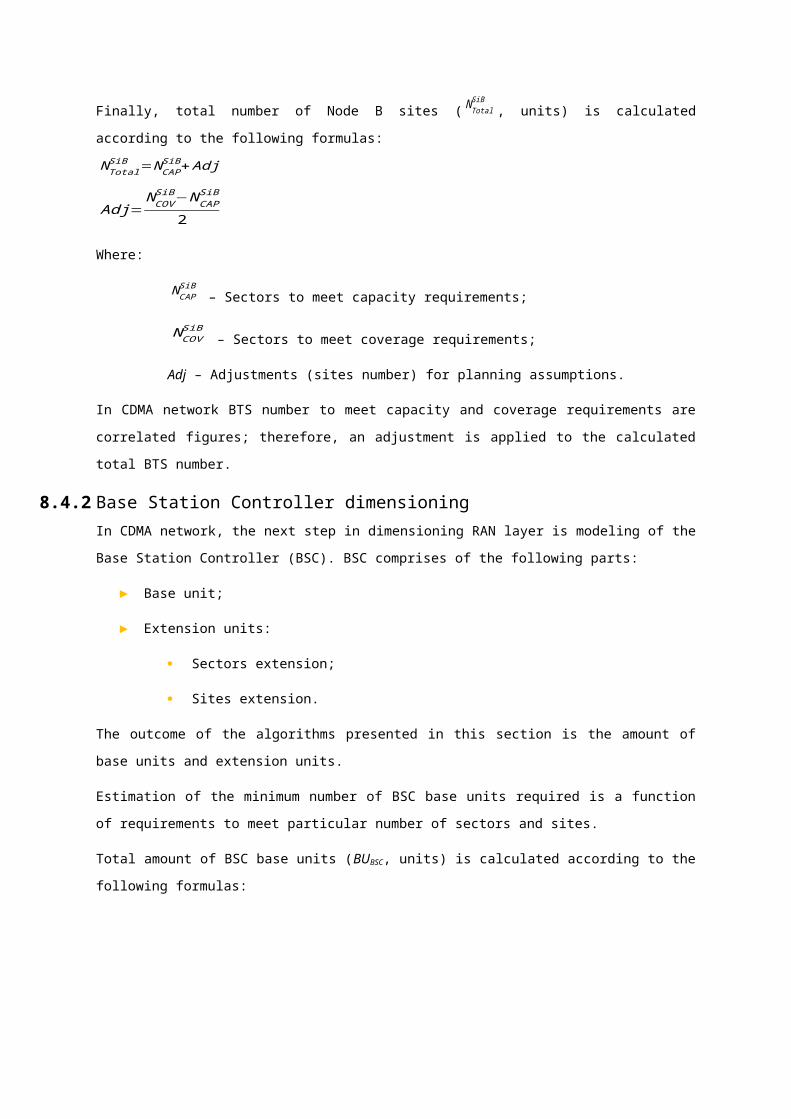
Total amount of Base Stations sites

Finally, total number of Node B sites (NTotalSiB

, units) is calculated according to the following formulas:NTotal

SiB =NCAPSiB +Adj

Adj=NCOV

SiB −N CAPSiB

2

Where:

NCAPSiB

– Sectors to meet capacity requirements;

NCOVSiB

– Sectors to meet coverage requirements;

Adj – Adjustments (sites number) for planning assumptions.

In CDMA network BTS number to meet capacity and coverage requirements are correlated figures; therefore, an adjustment is applied to the calculated total BTS number.

8.4.2 Base Station Controller dimensioningIn CDMA network, the next step in dimensioning RAN layer is modeling of the Base Station Controller (BSC). BSC comprises of the following parts:

► Base unit;

► Extension units:

Sectors extension;

Sites extension.

The outcome of the algorithms presented in this section is the amount of base units and extension units.

Estimation of the minimum number of BSC base units required is a function of requirements to meet particular number of sectors and sites.

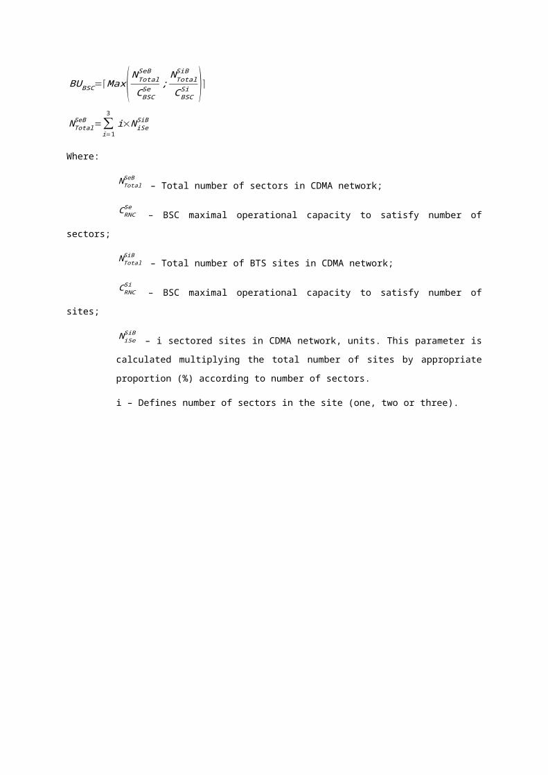
Total amount of BSC base units (BUBSC, units) is calculated according to the following formulas:

BU BSC=⌈Max ( NTotalSeB

CBSCSe ;

NTotalSiB

CBSCSi )⌉

NTotalSeB =∑

i=1

3

i×N iSeSiB

Where:

NTotalSeB

– Total number of sectors in CDMA network;

CRNCSe

– BSC maximal operational capacity to satisfy number of sectors;

NTotalSiB

– Total number of BTS sites in CDMA network;

CRNCSi

– BSC maximal operational capacity to satisfy number of sites;

N iSeSiB

– i sectored sites in CDMA network, units. This parameter is calculated multiplying the total number of sites by appropriate proportion (%) according

to number of sectors.

i – Defines number of sectors in the site (one, two or three).

8.5 Dimensioning the Ethernet distribution networkThe Ethernet distribution network covers the part of transmission network between Access Nodes and IP/MPLS layer.The approach we take to dimension the transmission network is similar to that taken for the Access Nodes in the following respects:

► It uses billed minutes and data traffic as the starting point;

► It incorporates holding times and an allowance for growth;

► It uses routing factors to determine the intensity with which each network element is used;

► It dimensions the network for the same busy hour as the Access Node’s network;

► It then adjusts this capacity to allow for flows between nodes and to provide resilience.

Dimensioning of the Ethernet distribution network is done in the following steps:► Access Node’s is equipped with Ethernet interfaces for backhaul purposes;

► Access Nodes are connected with Ethernet rings to Ethernet switch.

► Volume and capacity of Ethernet rings will be calculated based on the traffic volume generated by Access Nodes;

► Ethernet switch main unit (chassis) and expansion cards (GE, 10GE) volume will be calculated based on rings volume and capacity.

Dimensioning of Ethernet distribution network is calculated in these steps:1. For each Ethernet switch determine the main unit (chassis) type;2. For each Ethernet switch calculate the volume of expansion cards (GE, 10 GE,

switching cards).

8.5.1 Dimensioning of Ethernet switches main unitsThe main unit (chassis) type of Ethernet switch is determined based on the required capacity. It is assumed that there are 3 Types of chassis use in the network:Dimensioning of Ethernet Switches chassis Type 3 : NType−3ETH

=A+Max ( B ;C )

Where,

A=MAX (⌊ NT

CType 3ETHT

⌋; ⌊ N S

CType3ETH S

⌋)B=if ( NT−A⋅CType3ETHT

>CType 2ETH T

;1 ;0)C=if ( NS−A⋅CType 3ETH S

>CType2ETH S

;1 ;0)

Where,

NType−3ETH - Number of Ethernet Switch chassis Type 3;NT - Sum of Type 1, Type 2, Type 3 and Type 4 trunking cards with 1/10 GE interfaces;N S - Sum of switching cards;

Calignl ¿ Type3ETH T¿¿¿- Capacity of Ethernet Switch chassis Type 3, defined in volume of

1/10 GE cards;

Calignl ¿ Type2ETH T¿ ¿¿- Capacity of Ethernet Switch chassis Type 2, defined in volume of

1/10 GE cards;

Calignl ¿ Type3ETH S¿¿ ¿- Capacity of Ethernet Switch chassis Type 3, defined in volume of

switching cards;

Calignl ¿ Type2ETH S¿¿¿ - Capacity of Ethernet Switch chassis Type 2, defined in volume of

switching cards.

Dimensioning of Ethernet Switches chassis Type 2 : NType−2ETH

=A+MAX ( B;C )

Where,

A=MAX (⌊ NT−N Type−3ETH×CType3ETH T

CType 2ETH T

⌋;⌊ NS−NType−3ETH×CType3ETH S

CType2ETH S

⌋)B=if ( NT−Type3ETH⋅CType3ETH T

−A⋅CType2ETH T

>CType1ETHT

;1;0)C=if ( NS−Type3ETH⋅CType3ETH S

−A⋅CType 2ETH S

>CType1ETH S

;1 ;0)

Where,NType−2ETH - Number of Ethernet Switch chassis Type 2;



1/10 GE cards;


1/10 GE cards;

Calignl ¿ Type1ETHT¿ ¿¿- Capacity of Ethernet Switch chassis Type 1, defined in volume of 1/10

GE cards;


switching cards;


switching cards;


switching cards.

Dimensioning of Ethernet Switches chassis Type 1:

NType−1ETH=MAX (0 ; A ;B )

Where,

A=⌈N T−NType−3ETH

×CType3ETH T

−N Type−2ETH×CType2ETH T

CType1ETHT

⌉

B=⌈N S−NType−3ETH

×CType 3ETHS

−NType−2ETH×CType 2ETH S

CType1ETH S

⌉

Where,NType−1ETH - Number of Ethernet Switch chassis Type 1;NType−3ETH - Number of Ethernet Switch chassis Type 3;



1/10 GE cards;


1/10 GE cards;

Calignl ¿ Type1ETHT¿ ¿¿- Capacity of Ethernet Switch chassis Type 1, defined in volume of 1/10

GE cards;


switching cards;


switching cards;

Calignl ¿ Type1ETH S¿¿¿- Capacity of Ethernet Switch chassis Type 1, defined in volume of

switching cards.

8.5.2 Calculation of expansion cards of Ethernet switchCalculation of volume of expansion cards (GE, 10 GE, switching cards) for each Ethernet switch is based on the volume of traffic and the required amount of 1-10GE ports.Dimensioning of Ethernet Switches Switching cards:

N S=⌈V Tr

HA×CSCETH ⌉

Where,

CSCETH

- Capacity of Ethernet switching card in Gbit/s;V Tr - Total volume of traffic passing Ethernet switching network. Total traffic consists of traffic generated by Access Nodes, high speed leased lines, data traffic outgoing to POI, traffic forwarded to IP/MPLS network layer;

HA - Headroom allowance for Ethernet switch switching cards.

Dimensioning of Ethernet Switches Type 2 1GE cards:

NType−2ETH−1GE=⌊ 1GEEdgeETH

CType21GE ⌋+if (1GEEdgeETH−⌊ 1GE EdgeETH

CType 21GE ⌋×CType21GE>CType11GE ;1;0)Where,

NType−2ETH−1GE

- Number of Type 2 1GE cards;CType11GE - Capacity of Type 1 1GE cards, defined in 1GE interfaces;CType21GE - Capacity of Type 2 1GE cards, defined in 1GE interfaces;

1GEEdgeETH - Required volume of 1GE ports;

Dimensioning of Ethernet Switches Type 1 1GE cards :

NType−1ETH−1GE=⌈

1GE EdgeETH−NType−2ETH−1GE×CType21GE

CType11GE⌉

Where,

NType−1ETH−1GE

- Number of Type 1 1GE cards;

NType−2ETH−1GE

- Number of Type 2 1GE cards;CType11GE - Capacity of Type 1 1GE cards;CType21GE - Capacity of Type 2 1GE cards, defined in 1GE interfaces;

1GEEdgeETH - Required volume of 1GE ports.

Dimensioning of Ethernet Switches Type 4 10GE car d:

NType−4ETH−10GE=⌊10GEEdgeETH

CType 410GE ⌋+if (10GEEdgeETH−⌊10GEEdgeETH

CType 410GE ⌋×CType410GE>CType310GE ;1 ;0) Where,

NType−4ETH−10GE


10GEEdgeETH - Required volume of 10GE ports.

Dimensioning of Ethernet Switches Type 3 10GE cards :

NType−3ETH−10GE=⌈

10GEEdgeETH−N Type−4ETH −10GE×CType410GE

CType 310GE⌉

Where,

NType−3ETH−10GE


NType−4ETH−10GE

- Number of Type 4 10GE cards;CType310GE - Capacity of Type 3 10GE cards, defined in 10GE interfaces;

CType410GE - Capacity of Type 4 10GE cards, defined in 10GE interfaces;

10GEEdgeETH - Required volume of 10GE ports;

8.5.3 Calculation of amount of 1GE and 10GE portsThe amount of 1GE and 10GE ports is calculated in a few steps described below. Calculation of amount of 1GE portsCalculation of 1GE ports for each Ethernet location is done using the following formula:

1GEEdgeETH=⌈N LL−services

ETH + NPOIETH+N AN

ETH+N LEETH

HA⌉

Where,

N LL−servicesETH

- Number of GE ports required by the leased line and data transmission services provided by Ethernet network.Error: Reference source not found

N POIETH

- Number of GE ports required by the POI services provided by Ethernet network.

N ANETH

- Number of GE ports required by Ethernet network to connect ANs.

N LEETH

- Number of GE ports required at Ethernet network to transfer traffic to upper layer IP/MPLS network.

The number of GE ports required at Ethernet switching network to connect to IP router switches is calculated:

N LEETH=⌈

V AN−ETH

T ringbackhaul

⌉

Where,T ringbackhaul - Backhaul ring’s throughput (1 Gbit/s);V AN−ETH - Volume of traffic outgoing from all AN connected to the LN in Gbit/s. This traffic consists of voice, internet access and leased lines services, with routing factors applied, provided at AN.

The amount of GE ports required for leased line services provided from Ethernet switching network is calculated:

N LL−servicesETH =⌈(V STM−ll service

+V Txservice )×RFNC ⌉

Where,V STM−llservice - Volume of SMT-LL services provided in LN area;V Txservice - Volume of data transmission services provided in LN area;

RFNC - Average utilization of network component.

The amount required by the POI services provided from Ethernet switching network is calculated:

N POIETH=⌈V wholesale×ρETH

POI ⌉

Where,

ρETHPOI

- Proportion of total POI bandwidth outgoing at Ethernet switching networks;V wholesale - Volume of internet access services to wholesale subscribers;

The number of GE ports required at Ethernet switching network to connect ANs is calculated:

N ANETH=N ring−AN×2

Where,N ring−AN - Number of rings connecting ANs.

The number of rings connecting AN is calculated using the following formula:

N ring−AN=min(⌈N AN

N AN−ring⌉ ;max AN )

Where,N AN - Number of ANs connected to the LN location;N AN−ring - Maximal number of ANs connected to a ring at Local Node area.max AN - Predefined maximal number of ANs connected to a ring at Local Node area

The maximal number of ANs connected to a ring at Local Zone is calculated using the following formula:

N AN−ring=⌊ T ringbackhaul−T IPTV

(V AN−ETH / N AN ) ⌋Where,

T ringbackhaul - Backhaul ring’s throughput (1 Gbit/);HA - Headroom allowance for backhaul ring;N AN - Number of MSANs/OLT/AETH connected to the LN location;

V AN−ETH - Volume of traffic outgoing from all AN connected to the LN in Gbit/s. This traffic consists of voice, internet access and leased lines services, with routing factors applied, provided at AN in Local Zone minus traffic outgoing at POI in LN area.

Calculation of amount of 10GE portsThe number of 10GE ports required at Ethernet switching network is using same alghoritms as described in paragraph above, taking into account volumes of 10 GE ports.

8.6 Dimensioning the IP/MPLS core networkIP/MPLS node can be calculated in as-is state (scorched node) or optimize state (scorched earth). In as-is state (scorched node) IP routers will replace Exchanges at the existing locations. In optimized state (scorched earth) IP routers will be located in the main cities where POI is provided. However, the following calculation formulas apply in dimensioning using both approaches – scorched earth and node. In order to dimension Local nodes, the following assumptions have to be taken:

► Locate IP routers in the main cities of Numbering Zones.► Assign aggregation Ethernet Switches to Numbering Zones.

After an assumption takes place, dimensioning the number of the required IP routers is calculated in these steps:

1) Calculation of required number of ports for each IP router.

2) Calculation of volume of IC traffic for each IP router and MGW, based on services traffic volume and routing factors.

3) Determination of main unit (chassis) types of each MGWs based on the number and required capacity IC ports.

4) Calculation of number of expansion cards (E1, STM-1, GE) for each MGW.

5) Determination of main unit (chassis) types for each Core IP router based on the number of ports and the required capacity.

6) Calculation of number of expansion cards (GE, 10 GE, routing expansion, management) for each Core IP router.

8.6.1 Calculation of number of ports of IP routerThere are two types of ports in IP routers: 10GE short range and 10GE long range. Therefore, the total amount of required ports is the sum of 10GE ports for LN location. It is calculated using the following formula:

10GELN=N10GESR−LN+N10GE

LR−LN

Where,

10GELN - Total required number of 10GE ports in IP router at LN location;

N10GELR−LN

- Number of long range 10GE ports in LN location;

N10GESR−LN

- Number of short range 10GE ports in LN location;Calculation of 10GE short range portsThe number of required of 10GE short range ports in LN location is calculated using the following formula:

N10GESR−LN=⌈

GELN− peering+GEmgw−LN+GECES

HA⌉

Where,GE LN− peering - Number of GE interfaces used in LN for transferring data to peering points;GEmgw−LN - Number of GE interfaces required for MGW for IC traffic handling;HA - Headroom allowance of IP router trunking cards;GECES - Number of GE interfaces present at Ethernet switching network connected to LN location.

Number of GE interfaces used for data transfer to peering points is calculated using the following formula:

GELN−peering=⌈∑ (V STM−LL+V ATM )×RFNC ⌉+⌈∑ V WIA×RFNC ⌉

Where,RFNC - Average utilization of the appropriate network component;V STM−LL - Volume of traffic from high speed leased lines in Gbit/s; V WIA - Volume of services at LN location;V ATM - Volume of traffic from data transmission services in Gbit/s;

Volumes of traffic of the mentioned services are calculated using the following formula:

V STM−LL / ATM=V Tx−service×T x−Kbit /s

10242

Where,T x−Kbit /s - Average throughput per port of appropriate data service in Kbit/s; V Tx− service - Volume of services (STM-LL or ATM) provided at LN location.

The services volume is calculated using the following formula:

V Tx− service=round (V Tx− sercice input

V Tx−serviceinput−total×∑ ( Sservice−total )−V Tx−serviceinput−total; 0)+V Tx−serviceinput

Where,

V Tx− sercice .input - Volume of services (STM-LL or ATM) provided at LN location (input data);V Tx− sercice .input−total - Total volume of services (STM-LL or ATM) provided at LN location (input data);Sservice−total - Total amount of service (STM-LL or ATM) subscribers (input data).

Volumes of V Tx− sercice .input , V Tx− sercice .input−total and Sservice−total will be gathered via questionnaire from the operator.

Volume of Wholesale Internet Access services traffic outgoing the network (V WIA ) is calculated using the following formula:

V WIA=( ρ IA−to−service×T x−Kbit / s×N IA )×ρPOI−IP

10242

Where,ρ IA−to−service - Proportion of internet access services to wholesale subscribers;T x−Kbit /s - Average throughput per port of appropriate data service;N IA - Number of Internet Access services present at LN location;ρPOI−IP - Proportion of POI traffic outgoing at IP routers level.

The number of short range GE interfaces required for Ethernet switch connected to LN location is calculated using the following formula:

GECES=⌈V ETH− IP

HA×10⌉

Where,V ETH−IP - Traffic incoming from Ethernet switching layer to Local Nodes. This traffic is calculated by summing the volume of traffic incoming into Ethernet Switches minus the volume of traffic which is outgoing from the Ethernet switch layer;HA - Headroom allowance of Ethernet switches trunking cards.

Calculation of 10GE long range ports:The number of required of 10GE long range ports in LN location is calculated using the following formula:

N10GELR−LN=⌈

10GELN−LN

HA⌉×2

Where,HA - Headroom allowance of IP router trunking cards;10GELN −LN - Number of 10GE ports required in LN location to handle traffic generated by voice and data services.

The number of required 10GE ports in LN location to transfer data between Local Nodes

is calculated using the following formula:

10GELN −LN=⌈V LN−LN voice

+V LN−LN data

10 ⌉

Where,V LN−LN voice - Volume of traffic generated by voice services and traveling through LN;V LN−LN data - Volume of traffic generated by data services and traveling through LN;

Traffic generated by voice services is calculated using the following formula:

V LN−LN voice=∑ ( N l+NGPON /P2P )×VoIPbit−rate×mERLLN

1000×10242

Where,N l - Number of equivalent voice lines;NGPON /P2P - Number of GPON and Point to Point voice subscribers;VoIPbit−rate - VoIP channel bit rate;mERLLN - Average throughput per port for appropriate network component (NC). In this case for LN-LN network component.

Traffic generated by data services in Gbit/s going from LN location to other LN location (V LN−LN data ) is calculated by the following formula:V LN−LN data

=(∑ (V LL (64 ))+∑(V STM−LL))×RFNC+∑ (V IA )×RFNC+V IPTV

Where,RFNC - Average utilization of appropriate network component. See formula Error: Reference source not found;

V LL(64 ) - Volume of traffic from leased lines (analog, 2mb and nx64 leased lines) present at LN location. V STM−LL - Volumes of traffic of data services in Gbit/s present at LN location.V IPTV - Volume of traffic of IPTV services, estimated by converting the average throughput of IPTV services into Gbit/s;V IA - Volume of Internet Access services traffic in Gbit/s present at LN location;

Volume of Internet Access services traffic (V IA ) is calculated using the following formula:

V IA=∑ V residential+V bu sin ess+V wholesale

Where,

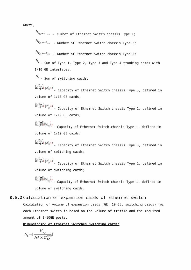
V residential - Volume of traffic generated by internet access services for residents;V bu sin ess - Volume of traffic generated by internet access services for businesses;V wholesale - Volume of traffic generated by internet access services for wholesale.

These internet access service volumes are calculated using the following formula:V int ernet access

=ρ xDsl−to−service×T x−Kbit /s×N IA

Where,V int ernet access - Volume of traffic generated by internet access services for residents, businesses or wholesale;ρxDsl−to− service - Proportion of Internet Access services provided for appropriate user (resident, business, wholesale);T x−Kbit /s - Average throughput per port of appropriate data service. N IA - Number of Internet Access services at LN location.

The volume of traffic aggregated from leased lines is calculated using the following formula:V LL(64 )=∑ (V ana log+V nx 64+V 2mb )Where,

V i - Volume of traffic coming from i lines (analog, nx64 or 2mb). See formula Error: Reference source not found.

This volume is calculated using the following formula:

V i=N i×T i−Kbit / s

10242

Where,T i−Kbit / s - Average throughput per port of appropriate data service;N i - Number of leased i lines (analog, nx64 or 2mb) present at LN location.

The number of leased lines present at LN location is calculated using the following formula:

N i=if ((SLL− S−∑ N i−pre lim )≥Rank ;1 ;0 )+N i−pre lim

Where,SLL−S - Total amount of leased lines service provided by the operator (input parameter);Rank - Rank of the N l lines present at LN location with leased lines services;N i−pre lim - Preliminary amount of leased lines service present at LN location.

Amounts of leased lines will be gathered from operator via questionnaireThe preliminary amount of leased lines at LN location is calculated using the following

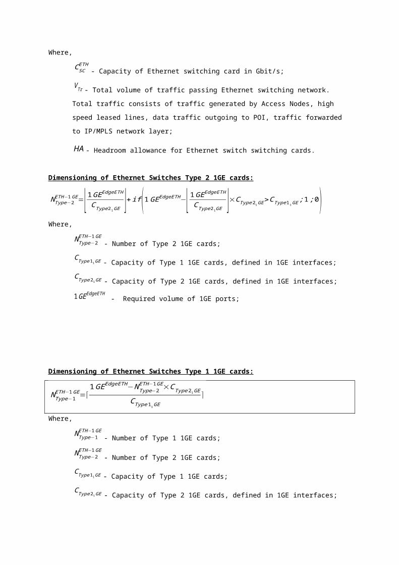
formula:

N i−pre lim=N l

∑ N l

×Si

Where,Si - Volume of leased line services in the selected year;N l - Number of leased line services present at LN location with leased lines services.

8.6.2 Calculation of IC ports of MGWFor each MGW calculate the required number of IC ports.The number of GE interfaces is calculated using the following formula:

GELN−MGW=MAX (minLN−MGW ;⌈ERLLN−POI×VoIPbit−rate

10242⌉ )

Where,GELN−MGW - Number of GE interfaces required for MGW for IC traffic handling;min LN−POI - Minimal number of LN-MGW interfaces, it is assumed that at least one GE interface is required between LN and MGW.ERLLN−POI - Traffic from LN to POI in erlangs.VoIPbit−rate - VoIP channel bit rate. See formula.

8.6.3 Determination of MGW main units

For each MGW the main unit (chassis) type based on IC ports number and the required capacity is determined. Chassis type and amount is determined using the following formula:

N MGW=⌈∑i=1

5

( N type−xMGW )

CCSC⌉

Where,N MGW - Number of MGW chassis;CCSC - Slot capacity of MGW chassis;

N type− xMGW

- Number of x type cards;x - Type of expansion card for MGW chassis, one of five types;

8.6.4 Calculation of expansion cards of MGWsFor each MGW calculate volume of expansion cards (E1, STM-1, GE). There are 5 types of

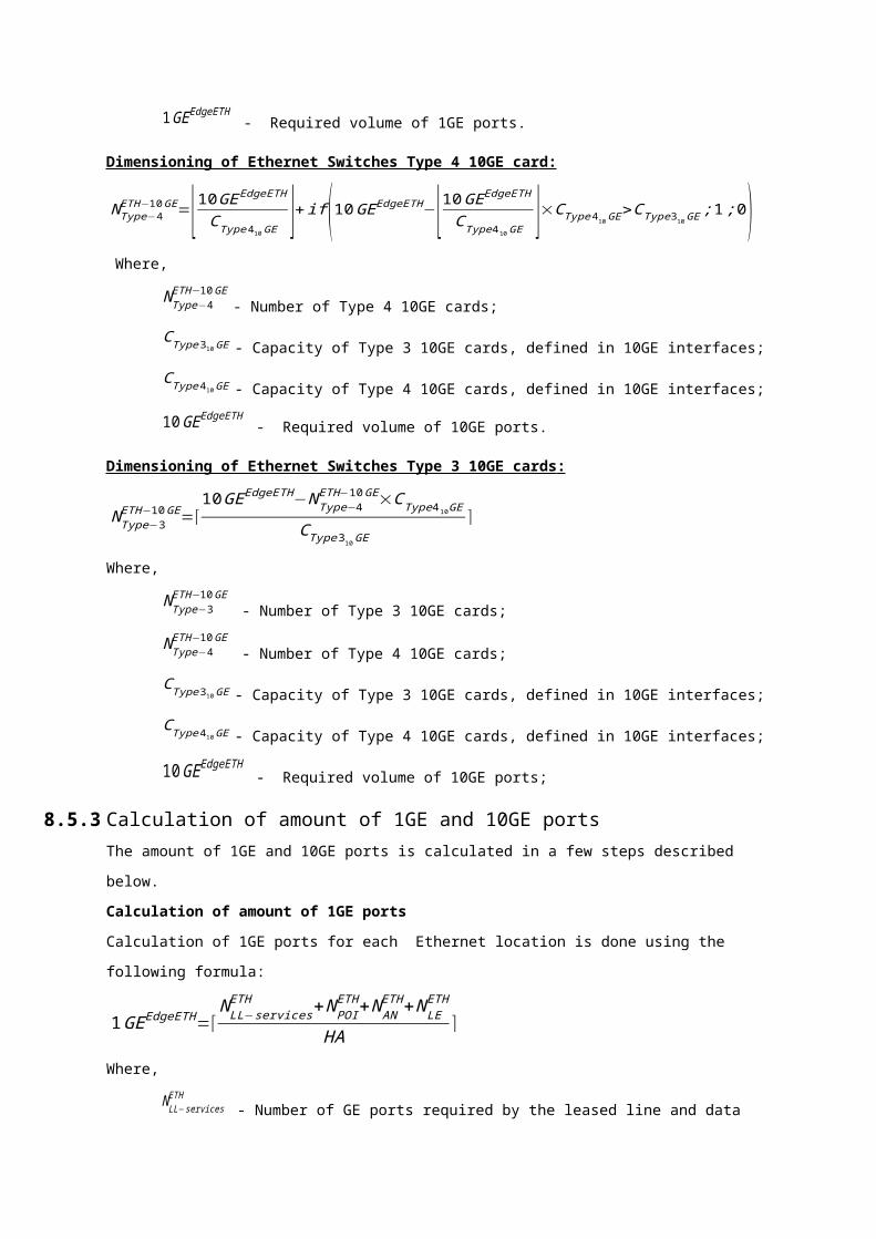
trunking/expansion cards which support different interfaces and voice processing card. Below formulas for dimensioning of each Type of cards are provided. Dimensioning of MGW expansion cards Type 1:

NType1MGW=max (

E1MGW−POI× ρE1−POI

HA−NType2

MGW×CType 2

CType 1;0 )

Where,

NType1MGW

- Number of Type 1 MGW trunking cards;HA - Headroom allowance for MGW trunking cards; CType1 - Capacity of Type 1 trunking card measured in E1 interfaces; CType2 - Capacity of Type 2 trunking card measured in E1 interfaces;ρE1−POI - Proportion of E1 interfaces joining MGW and POI;E1MGW−POI - Number of E1 interfaces connecting MGW and POI. This element is calculated in formula Error: Reference source not found;NType2

MGW - Number of Type 2 MGW trunking cards.

The number of E1 interfaces (E1MGW−POI ) is calculated using the following formula:

E1MGW−POI=ERLLN−MGW

C2mbit−linkWhere,

C2mbit−link - Capacity of 2Mbit/s link in Erlangs;ERLLN−MGW - Traffic in erlangs between LN and MGW.

This traffic is calculated using the following formula:

ERLNC=( N l−NC+NGPON /P2P)×mERLNC

1000Where,

ERLNC - Volume of traffic in ERL between appropriate network components;N l−NC - Number of MSAN equivalent voice lines aggregated by LN;NGPON /P2P - Number of GPON and Point to Point voice lines aggregated by LN ;mERLNC - Average throughput of the appropriate network component.

Dimensioning of MGW expansion cards Type 2:

NType2MGW=A+if (

E1MGW−POI×ρE1−POI

HA−A×CType2>CType1 ;1)

Where,

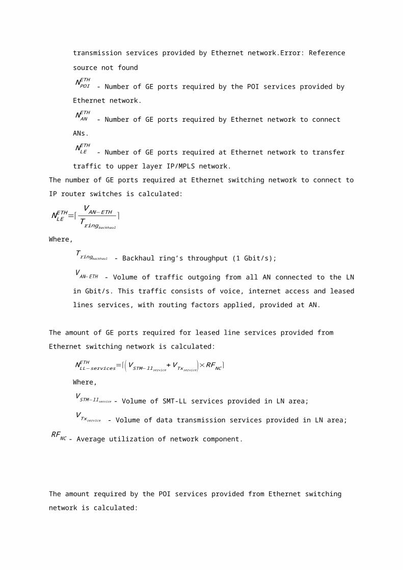
A=⌊ E1MGW−POI× ρE1−POI

HA×C Type2 ⌋ ;E1MGW−POI - Number of E1 interfaces connecting MGW and POI;ρE1−POI - Proportion of E1 interfaces joining MGW and POI;CType1 - Capacity of Type 1 trunking card measured in E1 interfaces;CType2 - Capacity of Type 2 trunking card measured in E1 interfaces;HA - Headroom allowance for MGW trunking cards;


NType3MGW=⌈

E1MGW−POI×ρSTM 1−POI

HA×CType3×CPOI−STM 1⌉

Where,NType3

MGW - Number of Type 3 MGW trunking cards, rounded up to the nearest

integer;E1MGW−POI - Number of E1 interfaces connecting MGW and POI;ρSTM 1−POI - Proportion of STM-1 interface joining MGW and POI;HA - Headroom allowance for media gateway trunking cards;CType3 - Capacity of Type 3 trunking card measured in STM-1 interfaces;CPOI−STM 1 - Capacity of SMT-1 interfaces in POI measured in E1 interfaces.


NType 4MGW=⌈

E1MGW−POI×ρSTM 4−POI

HA×CType4×C POI−STM 4⌉

Where,NType 4

MGW - Number of Type 4 MGW trunking cards;

E1MGW−POI - Number of E1 interfaces connecting MGW and POI;ρSTM 4−POI - Proportion of STM-4 interface joining MGW and POI;HA - Headroom allowance for media gateway trunking cards;CType4 - Capacity of Type 4 trunking card measured in STM-4 interfaces;CPOI−STM 4 - Capacity of SMT-4 interfaces in POI measured in E1 interfaces.

Dimensioning of MGW expansion cards to support GE interfaces:

NGEMGW=⌈

GELN−MGW

CGE−card⌉

Where,NGE

MGW - Number of GE MGW trunking cards in MGW;

CGE−card - Capacity of GE trunking card measured in GE interfaces;GETN−MGW - Number of GE interfaces connecting MGW with LN, rounded up to integer.

Dimensioning of MGW voice processing cards:

NVPMGW=⌈

ERLNC

HA×CVP⌉

Where,CVP - Capacity of voice processing card to handle erlangs;ERLNC - Volume of traffic in ERL between appropriate network components;HA - Headroom allowance for MGW switching cards.

8.6.5 Determination of main unit types of IP routerFor each IP router the main unit (chassis) type based on the number of ports and the required capacity is determined. The amount of each chassis is calculated using the following formula:NType−2 IP

=A+Max (B ;C )

Where,

A=MAX (⌊ NT

CType 2IP T

⌋;⌊ N S

CType2IPS

⌋)B=if ( NT−A⋅CType2 IPT

>CType1IPT

;1 ;0)C=if ( NS−A⋅CType 2IP S

>CType1 IPS

;1 ;0)

Where,

NType−2 IP - Number of IP router chassis Type 2;NT - Sum of Type 1 and Type 2 trunking cards with 10 GE interfaces;N S - Sum of switching cards;

Calignl ¿ Type2 IPT¿¿¿ - Capacity of IP router chassis Type 2, defined in volume of 10 GE

cards;

Calignl¿ Type1 IPT¿¿¿- Capacity of IP router chassis Type 1, defined in volume of 10 GE cards;

Calignl ¿ Type2IPS¿¿¿- Capacity of IP router chassis Type 2, defined in volume of switching

cards;

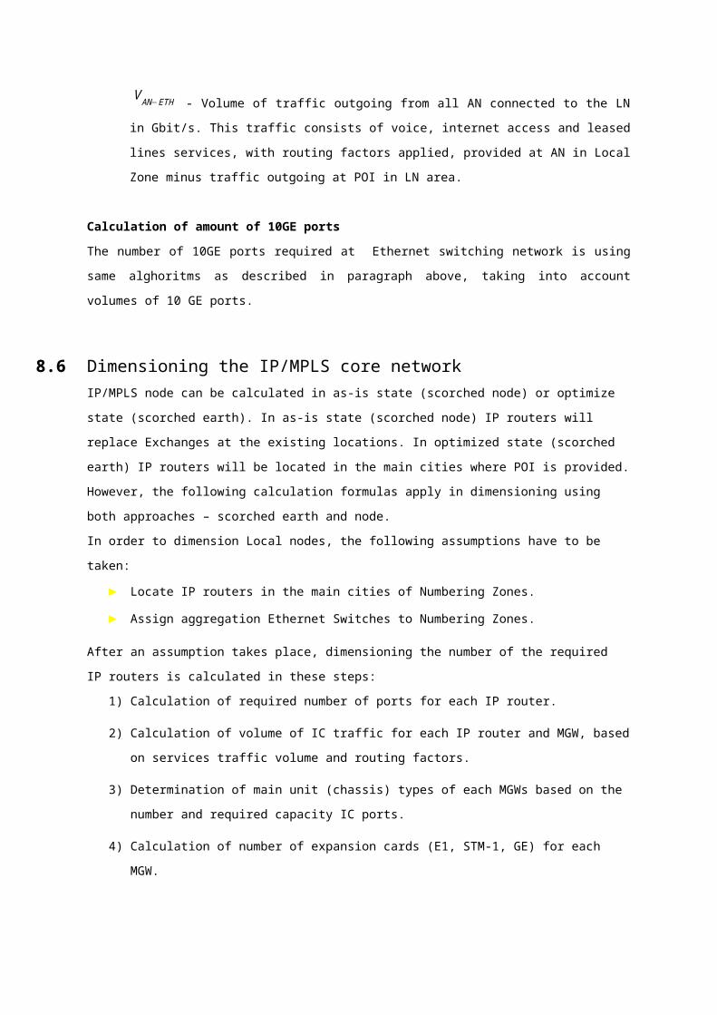
Calignl¿ Type1 IPS¿¿¿- Capacity of IP router chassis Type 1, defined in volume of switching

cards.

8.6.6 Calculation of IP router expansion cards It is assumed that there is on type of switching card and two types of trucking cards.

Dimensioning of IP routers Switching cards:

N S=⌈V Tr

HA×CSCIP ⌉

Where,

CSCIP

- Capacity of core IP routes switching card in Gbit/s;V Tr - Sum of all the traffic going through the IP router in Local Node location in Gbit/s divided by headroom allowance (HA). It consists of traffic outgoing to MGW and peering points as well as voice and data traffic between LNs;

HA - Headroom allowance for IP routes switching cards.

Dimensioning of core IP router Type 2 10GE card:

NType−2IP−10GE=⌊10GEIP

CType210GE ⌋+ if (10GE IP−⌊10GE IP

CType210GE ⌋×CType 210GE>CType110GE ;1; 0) Where,

NType−2IP−10GE


10GEIP - Required volume of 10GE ports;

Dimensioning of core IP router Type 1 10GE cards:

NType−1IP−10GE=⌈

10GEIP−NType−2IP−10GE×CType210GE

CType 110GE⌉

Where,

NType−1IP−10GE


NType−2IP−10GE

- Number of Type 2 10GE cards. See formula Error: Reference source notfound;CType110GE - Capacity of Type 1 10GE cards, defined in 10GE interfaces;

CType210GE - Capacity of Type 2 10GE cards, defined in 10GE interfaces;

10GEIP - Required volume of 10GE ports. See formula Error: Reference source

not found.

8.6.7 Home Location Register and Centralized User Database (CUDB)The Home location register (HLR) and Centralized User Database (CUDB) comprises two parts:

► Base unit;► Extension units.

The number of HLR and CUDB main and extension units is calculated based on the volume of CDMA subscribers.

8.7 Dimensioning of the transmission network passive elements8.7.1 Dimensioning the fiber cables

Dimensioning of the fiber cables requires to calculate the length of the fiber cables in each defined level of the transmission network (local and transit). Fiber cables length will be obtained from the operator (as is state) and verified based on the geographical coordinates of network nodes and logical topology of the network (optimized state). For fiber cable costs the fixed (e.g. cost of laying) and variable part (e.g. cost of fiber cable) would be established based on the economical data on individual network elements gathered from operators.

From the traffic-related costs only the variable part of the fiber cable cost which would be avoided in the absence of a service being provided should be allocated to the relevant increment proportionally to the traffic volume.

Fiber cables CVR – Cost Volume Relationship

The cost of fiber cables will be driven by the required throughput of cable section. To simplify the model, a linear relationship between the fiber cables cost and the fiber cables throughput is assumed. To find the relationship, two boundary points are defined:

1) Minimal network cost – cost of fiber network dimensioned to fulfill only topology requirements, traffic volume is not taken into account. The minimal fiber network cost may consist of: fiber cables (with the minimal number of fibers)) cost, joints cost and installing cost.

2) Nominal network cost – cost of fiber network dimensioned to fulfill the topology and traffic requirements. The nominal fiber network cost may consist of: fiber cables (with the nominal number of fibers)) cost, joints cost and installing costs (these statistics are to be provided by the operator).

The graph presenting CRV of fiber cables is presented below.

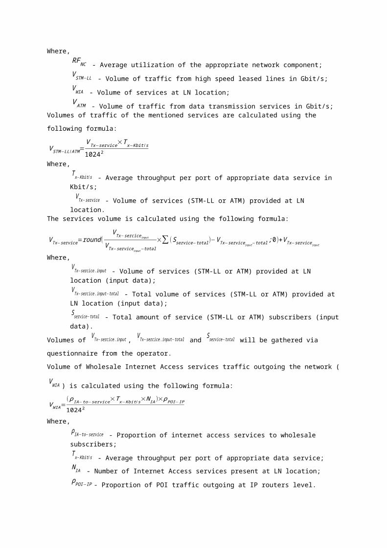
Minimal network

Nominal network

Fiber cable cost

Troughtput

Incremental costdriven by troughtput

Therefore the costs of fiber cables in the operating network would be the difference between the two scenarios listed above.

8.7.2 Dimensioning the ductsDucts length will be obtained from the Operator (as is state) and verified based on the geographical coordinates of network nodes and the logical topology of the network (optimized state). For duct costs the fixed (e.g. cost of digging, surface reconstruction) and variable part (e.g. cost of ducts) would be established based on the economical data on individual network elements gathered from operators. From the traffic-related costs only the variable part of ducts cost, which would be avoided in the absence of a service being provided, should be allocated to the relevant increment proportionally to the fiber cable incremental cost.

Ducts CVR – Cost Volume Relationship (rural)

The cost of ducts in rural genotypes will be driven by the cost of fiber cables. The CVR function defined for fiber cables would be used, however, two boundary points for ducts cost must be defined:

1) Minimal network cost – cost of ducts dimensioned to fulfill only topology requirements, traffic volume is not taken into account. The minimal ducts cost may consist of: trench cost, ground reconstruction cost and other earth work cost.

2) Nominal network cost - cost of ducts dimensioned to fulfill topology and traffic requirements. The nominal ducts cost may consist of: primary duct cost (nominal number of bores in rural) manholes cost, ground reconstruction cost and other earth works cost (these statistics are to be provided by the operator).

Ducts CVR – Cost Volume Relationship (urban)

Cost of ducts in an urban geotype will be driven by the cost of fiber cables. The CVR function defined for fiber cables would be used, however, two boundary points for ducts cost must be defined:

1) Minimal network cost – cost of ducts dimensioned to fulfill only topology requirements, traffic volume is not taken into account. The minimal ducts cost may consist of: trench cost, ground reconstruction cost and other earth work cost.

2) Nominal network cost - cost of ducts dimensioned to fulfill topology and traffic requirements. The maximal ducts cost may consist of: primary duct cost (nominal number of bores in urban) manholes cost, ground reconstruction cost and other earth works cost (these statistics are to be provided by the operator). The graph presenting CRV of ducts is presented below.

Minimal network

Nominal network

Duct cost

Fiber cost

Incremental costdriven by f iber CVR

8.7.3 Algorithm of the passive network length calculation.Algorithm of the fiber network length calculation can be divided into following steps:

► Aggregation of Access Nodes in cities► Division of cities in Numbering Zones into groups ► Optimization of ring networks in groups► Optimization of network at regional and national levels.► Calculation of road distances for all connections

Above steps are presented on the scheme below:

Aggregation of points in cities

Division of cities inthe Numbering

Zones into groups

• Preparation of an unique list of cities

• Counting of Subscriber Access Points and calculation of the coordinates representing each city

• Calculation of the length of network within city

Optimization ofring networks in

groups

Optimization of network atregional and national levels

• Calculation of the number of groups in each Numbering Zone

• Classification of cities into groups in each Numbering Zone with centroid based algorithm

• Definition of “connectors” – points that connect each group within the Numbering Zone

• Optimal design of ring networks in groups (in each Numbering Zone) with an algorithm that solves the travelling salesmen problem.

• Inclusion of the nearest points representing the Numbering Zones into predefined transit network

• Connecting remaining points representing the Numbering Zones into adjusted transit network

Aggregation of points within the boundaries of cities

In the first stage of the optimization process, a list of unique locations (cities) is created on the basis of the list of the Access Nodes. For each city the number of the Access Nodes is assigned, as well as the coordinates that will represent city and length of the network within the city – between aggregated Access Nodes.

In case the infrastructure operators provide sufficient data, the length of each city’s network will be calculated using the following algorithms:

► for cities having 2 and 3 Access Nodes – Access Nodes are connected directly;

► for cities having more than 3 Access Nodes - Access Nodes are connected using algorithm

that solves the travelling salesmen problem (described in point no 3).

Division of cities in the Numbering Zones into groups

For each Numbering Zone, all cities that represent Access Nodes, will be divided into groups, in which they will be connected into optimal ring networks.

The algorithm of the division into groups is based on the centers of gravity (centroids) method. At the beginning for each group a random point is chosen. This points are called centers of gravity.

In each iteration, each city is assigned to the nearest center of gravity. Then for each center of gravity is calculated a point with average coordinate of points assigned to specified center of gravity. Such points become new centers of gravity in next iteration. The algorithm is repeated until the stable solution is acquired – when the coordinates of centers of gravity do not change in following iterations.

Selection of random points – Assigning of cities to the

initial centers of gravity nearest centers of gravity

Calculation of new centers of gravity

Reclassification of cities with new centers of gravity

Next, in case the cities are divided into two or three groups, from each group there is chosen a city, that will be potentially a “connector” between the networks (groups) in the boundary of a Numbering Zone. If there are only two groups, then the algorithm chooses two nearest points from both groups and adds a point from the second group to the list of points in the first group. In case there are three groups, the algorithm will chose from each pair of groups a pair of nearest points.

Group 1

Group 2

d23

d12

d13

2a

1b

1a

3a

2b

d12

d23 d13

Group 3

1b

1a 2a

2b

3a 3b

The pair of points with the longest distance between them will be rejected, while two points from the remaining two pairs will be included as the connectors of the networks, according with the following rules:

d12=max {d12 , d13 , d23 }→add point 3a¿ group1∧add point2b¿ group3

d13=max {d12 , d13 , d23 }→add point2a¿ group1∧add point2b¿ group3

d23=max {d12 , d13 , d23 }→add point2a ¿ group1∧add point1b¿ group3

Optimization of ring networks for groups of cities within the Numbering Zones.

In each Numbering Zone, for each group of cities the ring network will be optimized. Implemented algorithm is based on the method developed by Durbin and Willshaw1.

This method uses an “elastic net”, that is strung initially as a ring within a boundary of analyzed area and in each iteration it adjusts to the distribution of cities. The network consists of points, which number is a multiplicity of the number of cities.

Initial shape of the elastic net

First iteration

1 Durbin R., Willshaw D., „An Analogue Approach to the Travelling Salesman Problem Using an Elastic Net Approach”, Nature, 326, 6114, pp 689-691, 1987.

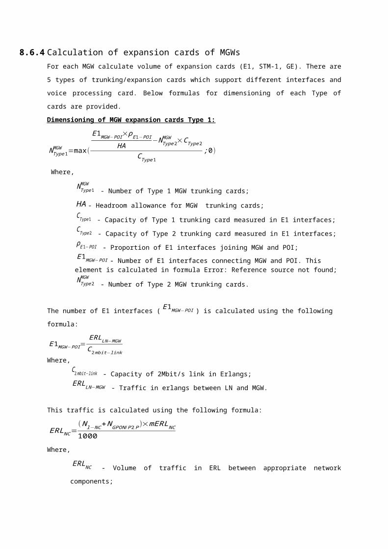
In each iteration a city is chosen randomly. For selected city the nearest point in the elastic net is chosen and “moved closer” towards the city. Also the adjacent points of the nearest point are moved towards selected city.

Iterative algorithm is repeated until the stable solution is found.

Iteration No. 10 Iteration No. 50 Iteration No. 100

Iteration No. 1000 Iteration No. 2430 (final)

In each iteration cities are selected randomly, hence it is possible to obtain suboptimal solution. Concerning mentioned above condition, whole algorithm is repeated multiple

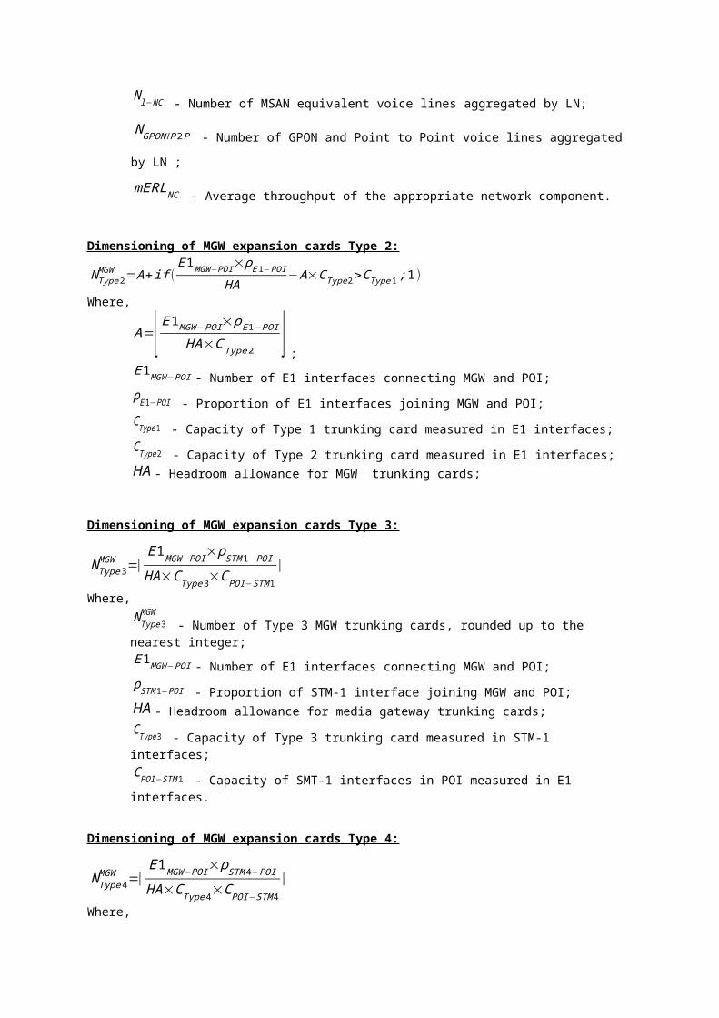
times in order to choose the best possible solution from the group of obtained results.

Optimal design of network at national and level

At the national level, initially the network is strung manually between Local Nodes. The network consists of two independent loops.

For each link between two nodes in the initial network is made a selection of points representing the numbering zones, that lie in the proximity of the links. Such points are included in the initial network.

In case of the other points representing the numbering zones, for each of them two links are made. First is stung between such point and the nearest point in the network. Second link is established between selected point and the nearest point in the network (but not to the point to which it is already connected by the first link) or the nearest point that was not initially connected. Then the doubled connections are deleted in order to create a list of unique links. In the iterative process, for each link is counted it’s length and number of links for each of connected node. In each iteration one link with more than two links connected to each of the nodes and the maximum length is deleted. The iterative process is repeated until there remains the minimum number of links.

Calculation of road distances for all connections.

For each connections dimensioned in point 1, 3, and 4 the algorithm calculates road distance.

8.8 Other network elements 8.8.1 IMS – IP multimedia subsystem

Dimensioning of IMS – IP multimedia sub-system, is done using the following steps: For the whole network calculate the volume of BHCA. The total BHCA for the network is calculated using the following formula:

BHCA=

V r⋅rBHT / AVG

365×24×Rl×(1+Rr )

HAWhere,

BHCA - Total busy hour call attempts in the network;rV - Total realized services volume;

AVGBHTr / - Busy Hour to Average Hour traffic ratio. Rr - Ratio of unsuccessful call attempts to total call attempts;Rl - Average call length;HA - Headroom allowance for IMS voice processing elements.

For the whole network calculate the volume of BHE. Total volume of Busy hour erlangs is

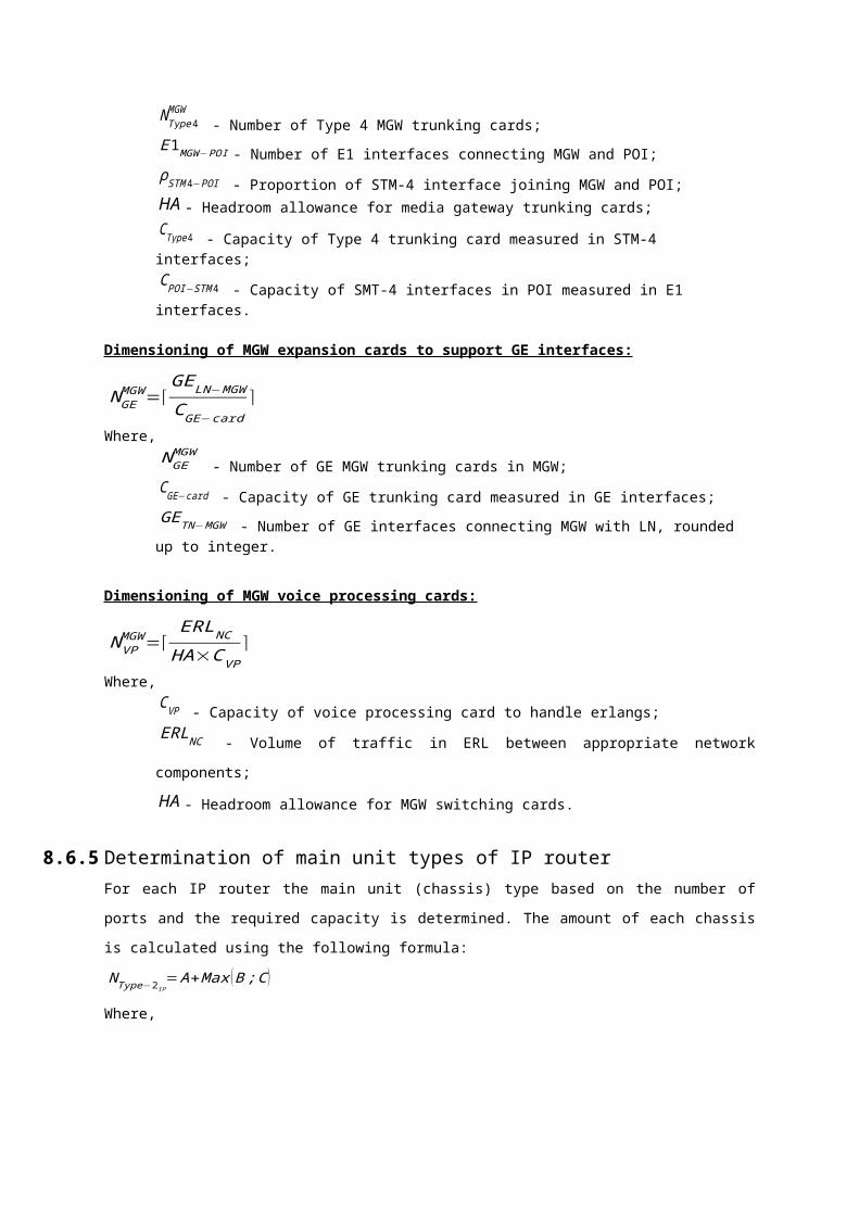
calculated using the following formula:

BHEIMS=mERLAN×N l−total

1000×HAWhere,

BHE IMS - Busy hour erlangs;mERLAN - Average throughput per port in Access Node;N l−total - Total amount of voice lines in Access Node network;HA - Headroom allowance for IMS voice processing elements.

For the whole network calculate the number of voice services. The following formula is used to calculate the total amount of voice services:

Stotal=N l−total

HAWhere,

Stotal - Total amount of voice services in the network;

totallN - Total amount of voice lines in Access Node network. It is calculated by summing all of the voice lines in the Access Node network;HA - Headroom allowance for IMS subscriber serving elements.

The volume of IMS extension cards (TDM processing, VoIP processing) are calculated according to the following algorithm:The number of required IMS Type 1, 2, 3, 4, 5, 6 cards is calculated using the following formula:

NType−xIMS =max ( ⌈

V z

Cx−capacity⌉;2 )

Where,Cx−capacity -Typex IMS service card handling capacity;V z - Total network volumez handled byx type of component;

z - Total network volume of BHE orBHCA orStotal ;x - IMS service card Type: 1 or 2 or 3 or 4 or 5 or 6.

The number of required HSS service cards is calculated using the following formula:

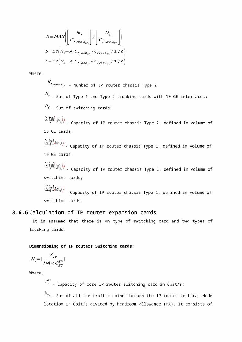
NType−1/2HSS =MAX (⌈

S total

Cx−capacity⌉;2 )

Where,Stotal - Total amount of voice subscribers in the network;C x−capacity - Typex HSS service card handling capacity;x - Type of the service card. There are two types in total.

8.8.2 Billing systemThe model will dimension only the network elements that participate in the provision of wholesale termination, origination and transit services; therefore, only the wholesale related part of the billing system will be dimensioned.Wholesale billing system encompasses the infrastructure from traffic data collection to invoicing and payment monitoring in particular hardware and software required for: ► Collecting and processing wholesale billing records;

► Warehousing of wholesale traffic data;

► Invoicing of wholesale customers.

The billing system is dimensioned using the following steps: Calculate the number of servers to support the required CDR. Calculations is done using the following formula:

N IC=⌈N IC−exp

C IC−M .capacity⌉

Where,

N IC- Number of billing system main units;

C IC−M .capacity - Billing system main unit’s slot capacity;N IC−exp - Number of IC system’s expansion cards.

The required amount of expansion cards is calculated using the following formula:

N IC−exp=⌈ CDRHA×C IC−Exp .capacity

⌉

Where,C IC−Exp .capacity - Expansion unit’s handling of BHE capacity;HA - Headroom allowance for IC hardware and software;

CDR - Call detail records to be handled by the billing system. This amount is estimated by summing the amount of interconnection traffic multiplied by its CDR statistics.

9. Network valuation

9.1 Cost annualizationAll fixed line network elements identified during network dimensioning are revalued at Gross Replacement Cost (GRC). On the basis of GRC value, its annual CAPEX cost is being further calculated. In BU-LRIC model there are four alternative methods that are used to calculate annual CAPEX costs:

► Straight-line method;

► Annuity method;

► Tilted Annuity method;

► Economic depreciation method.

Algorithms to calculate annual CAPEX cost (depreciation and ROI) using straight-line, annuity, tilted annuity and economic depreciation methods are described in the following sections. Straight-line methodThe annual CAPEX costs under the straight-line method are calculated according to the following formula:C=CD−HG+ROI

Where:

►

CD=GRCl

- current depreciation (l – useful life of an asset (data will be gathered from Operators); GRC –gross replacement cost of an asset);

►

HG=NBVGBV

GRC×index, holding gain (loss);

►

ROI= NBVGBV

GRC×WACC - cost of capital;

► Index - price index change (data will be gathered from Operators);

► NBV – net book value;

► GBV – gross book value;

► WACC - weighted average cost of capital.

Annuity methodThe annual CAPEX costs under the annuity method are calculated according to the following formula:

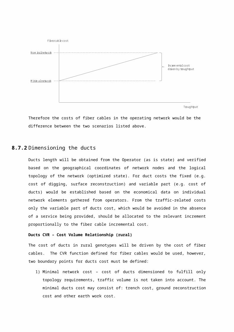
C=GRC (WACC )

1−( 11+WACC )

l

Tilted annuity methodThe annual CAPEX costs under tilted annuity method are calculated according to the following formula:

C=GRC (WACC−index )

1−( 1+index1+WACC )

l

Economic depreciation methodThe economic depreciation algorithm involves a cash-flow analysis to answer the question: what time-series of prices consistent with the trends in the underlying costs of production (e.g. utilization of the network, price change of asset elements) yield the expected net present value equal to zero (i.e. normal profit).Economic depreciation requires forecasting the key variables:

► Cost of capital;

► Changes in the price of Modern Equivalent Asset;

► Changes in operating cost over time;

► Utilization profile.

► The impact of key variables on depreciation is as follows:

► The lower the cost of capital, the lower the cost of investment that needs to be recovered in any year;

► The grater the future MEA price reductions, the more depreciation needs to be front-loaded;

► The deprecation should be brought forward, according to the increase of operating cost of an asset.

Economic depreciation is a method to calculate annual costs based on a forecasted revenue distribution during the useful asset lifetime. This is the main reason why this method is favored in theory. However, in the current BU-LRIC model the use of economic depreciation is excluded from modeling scope due to some reasons. Firstly, results from this method are highly dependable on various forecast assumptions. Forecasted revenue, cost of capital, changes in the price of Modern Equivalent Asset, changes in operating cost over time, utilization profile are essential for calculations, though having in mind the

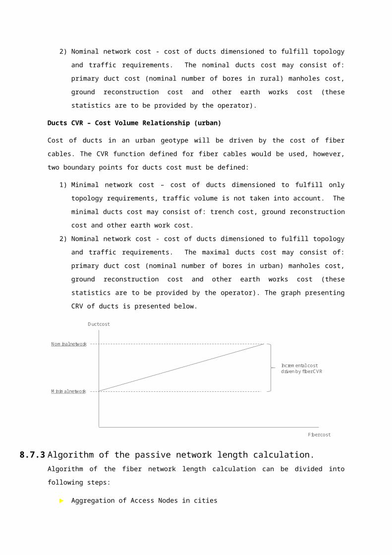
dynamic nature of the electronic communications market, forecasts may be subjective. Secondly, using alternative cost annualization methods, such as straight-line, annuity or tilted annuity, enables to reach comparable results.

The tilted annuity method will be used as the main method to calculate annual CAPEX costs due to simplicity and a fact that it generates a depreciation profile similar to that of economic depreciation – method recommended by Recommendation. It is worth mentioning that the model will have a possibility to calculate annual CAPEX using straight line, annuity and tilted annuity methods.

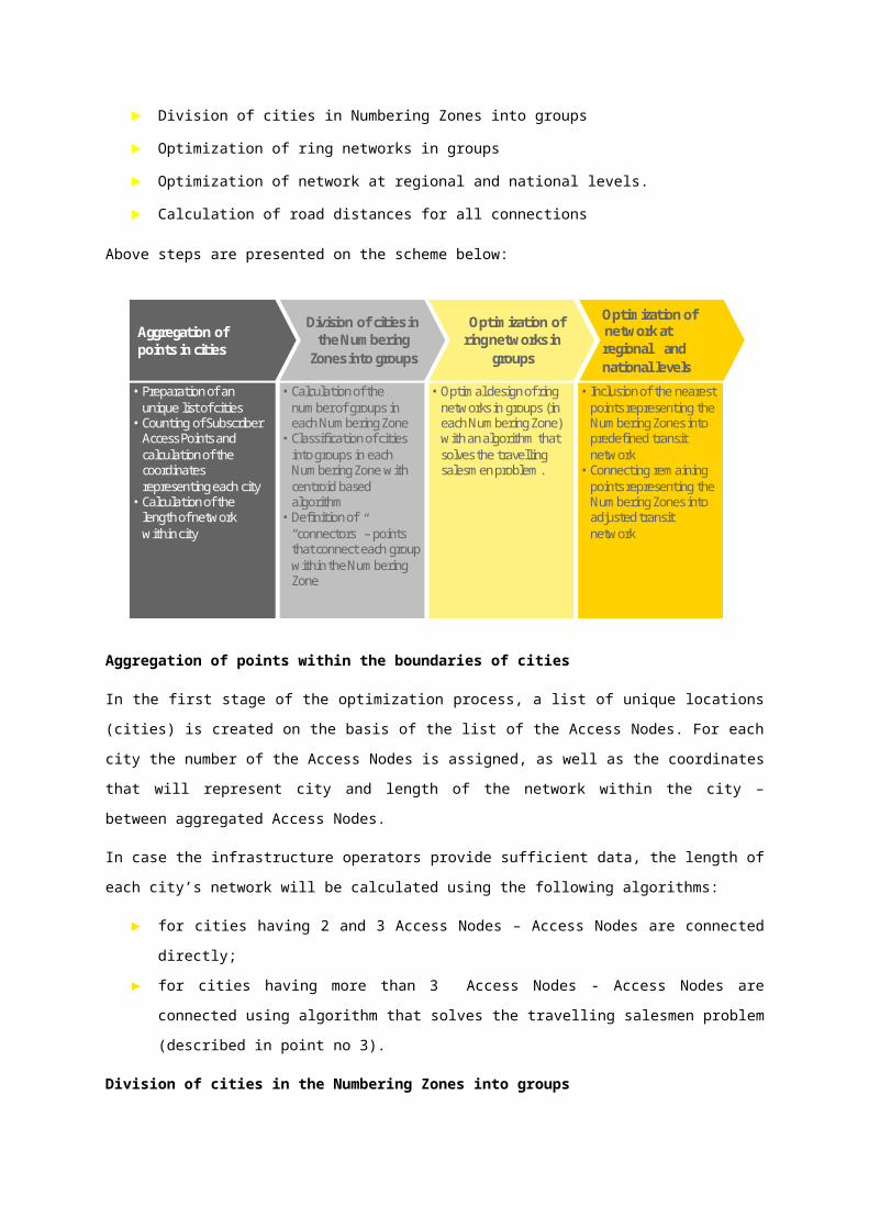
9.2 Mark-upsBU-LRIC models operational, NMS, administration and support costs as mark-ups of the network costs. In particular the following cost categories will be covered in the model as a cost rates:Operational cost categories

► Network operation, maintenance and planning expenses - operational costs of planning, management, on—site visits, inspections, configuration and maintenance works, for particular network elements:

► Access nodes

► Core network

► Fiber cables and ducts

► Operational cost of general administration, finance, human resources, information technology management and other administration and support activities (salaries, materials, services).

Capital cost categories► Network management system - general

► Network management system – dedicated to network elements

► Access node

► Core network

► Fiber cables and ducts

► Capital costs of general administration, finance, human resources, information technology management and other administration and support activities (buildings, vehicles, computers, etc.)

The above cost categories will be covered by calculating:► Mark-ups on network capital cost, or

► Mark-ups on network operational cost.

Markups on network capital cost would be calculated for the following cost categories:

► Network operation, maintenance and planning expenses (operational cost)

► Network management system – general (capital cost)

► Network management system – dedicated to network elements (capital cost)

Markups on network operational cost, previously allocated on corresponding network elements, would be calculated for the following cost categories:

► Capital costs of general administration, finance, human resources, information technology management and other administration and support activities.

► Operational cost of general administration, finance, human resources, information technology management and other administration and support activities.

The scheme below present mechanism of calculating cost which are based on cost rates.

Operational costNetwork operation, maintenance and planning expenses

Network GRC

NMS costNetwork management system - general

Network management system – dedicated to network elements

Operational costNetwork sites rental fees, Energy costs

Capital costLand and Buildings - Network Sites, Power plants

Rate of operational costs to network capital cost

Rate of operational cost to network operational

Rate of network management system cost to

network capital cost

Rate of capital cost to network operational cost

The mark-ups value will be calculated based on the financial data of operators.

10. Services costs calculation

10.1 Pure LRIC and LRIC approachThe avoidable costs of service (e.g. call termination) or group of services (e.g. voice calls) increment may be calculated by identifying the total long-run cost of an operator providing its full range of services and then identifying the long-run costs of the same operator in the absence of the service or group of services being provided to third parties and subscribers. This may then be subtracted from the total long-run costs of the business to derive the defined increment. The diagram below illustrates methodology of incremental cost calculation.

The incremental cost is calculated as follows:

U=NC (2 )−NC (1 )

V (2 )−V (1 )Where,

U – incremental costNC(1) – cost of network planned to utilize demand for V(1) service volume NC(2) – cost of network planned to utilize demand for V(2) service volumeNC(2) – NC(1) – incremental cost of network (avoidable cost)V(2) – total service volumeV(1) – total service volume less service or group of services volume V(2) –V(1) – service or group of services volume

10.2 LRIC+ approachWhen calculating costs using LRIC+ additional mark-ups are added on the primarily estimated increments to cover costs of all shared and common elements and activities which are necessary for the provision of all services. After establishing the incremental costs of Network Components (NC), the common and join cost (CJC) are allocated to the Network Components (NC) using equally-proportional mark-up (EPMU) mechanism based on the level of incremental cost incurred by each Network Component. Total Network Components costs are divided by service volumes and Network Component unit costs are calculated. And finally Network Component unit costs are multiplied by routing factor and service costs are calculated.

Documents

Report · Web viewCDMA 1x and EVDO for wireless fixed access. It is assumed that services provided over coaxial cables will be provided in the modeled network using fiber cables and