Embed Size (px)
Citation preview

SANDIA REPORT SAND2003-1887 Unlimited Release Printed June 2003
of
I
Y'S 85000.
ma National laboratories

lssued by Sandia National Laboratories, operated for the United States Department of Energy by Sandia Corporation.
NOTICE: This report was prepared as an account of work sponsored by an agency of the United States Government. Neither the United States Government, nor any agency thereof, nor any of their employees, nor any of their contractors, subcontractors, or their employees, make any warranty, express or implied, or assume any legal liability or responsibility for the accuracy, completeness, or usefulness of any information, apparatus, product, or process disclosed, or represent that its use would not infringe privately owned rights. Reference herein to any specific commercial product, process, or service by trade name, trademark, manufacturer, or otherwise, does not necessarily constitute or imply its endorsement, recommendation, or favoring by the United States Government, any agency thereof, or any of their contractors or subcontractors. The views and opinions expressed herein do not necessarily state or reflect those of the United States Government, any agency thereof, or any of their contractors.
Printed in the United States of America. This report has been reproduced directly from the best available copy.
Available to DOE and DOE contractors from U.S. Department of Energy Office of Scientific and Technical Information P.O. Box 62 Oak Ridge, TN 37831
Telephone: (865)576-8401 Facsimile: (865)576-5728 E-Mail reaorts(iiladonis.osti. eov Online ordering: httD://www.doe.eovibridee
Available to the public *om US. Department of Commerce National Technical Information Service 5285 Port Royal Rd Springfjeld, VA 22161
Telephone: (800)553-6847 Facsimile: (703)605-6900 E-Mail: orders(iilntis.fedworld. POV Online order: ht to : /~ .n t i s . eov~e lo /ordmnethods .as~?~o~7-4~~onl ine

SAND2003-1887 Unlimited Release Printed June, 2003
Projection of the Cost-Effectiveness of PIMs for
Particle Transport Codes Thomas W. Christopher Independent Consultant
1140 Portland Place #205 Boulder, Colorado 80304
Sandia Contract 301 17
Abstract
PIM (Processor in Memory) architectures are being proposed for future supercom- puters, because they reduce the problems that SMP MMPs have with latency. How- ever, they do not meet the SMP MPP balance factors. Being relatively processor rich and memory starved, it is unclear whether an ASCI application could run on them, either as-is or with recoding. The KBA (Koch-Baker-Alcouffe) algorithm (Koch, 1992) for particle transport (radiation transport) is shown not to fit on PIMs as written. When redesigned with a 3-D allocation of cells to PIMs, the resulting algorithm is projected to execute an order of magnitude faster and more cost-effectively than the KBA algorithm, albeit with high initial hardware costs.
Projecting Algorithm Performance 3

4 Projecting Algorithm Performance

Contents
Contents Acronyms and Abbreviations
Introduction
PIMS: What and Why?
Essentials of Particle Transport Algorithms
Fitting the applications on PlMs
Speculating about 3-D decompositions
Block allocation of cells to PlMs
Row-major allocation of cells to PlMs
Rod allocation of cells to PlMs
Overall cell update time
Fault Recovery
2D Decompositions on PlMs
Comparing to SMP Clusters
Conclusions
Further work
Formulae
References
7 9
9 14 22 24 33 40 43 49 50 52 57 63
64 66 70
Projecting Algorithm Performance 5

INTENTIONALLY LEFT BLANK
6 Projecting Algorithm Performance

Acronyms and Abbreviations
Acronyms and Abbreviations
KBA
MPP MPU PIM
Koch-Baker- Alcouffe algorithm for radiation transpodparticle transport, (Koch, 1992)
massively parallel processor micro-processing unit, microprocessor processor in memory or processing in memory chip
SMP shared-memory or symmetric multiprocessor SWEEP3D a benchmark implementation of the KBA algorithm
Projecting Algorithm Performance 7

INTENTIONALLY LEFT BLANK
8 Projecting Algorithm Perfbrmance

introduction
Introduction PIM (Processor in Memory) architectures are being proposed for future supercom- puters. They offer many more processors than conventional SMP clusters and MPP designs in the same number of chips. This allows their proponents to quote much higher FLOPS ratings, but they appear to have some limitations that may make them unusable. Here we evaluate whether PIMs have the potential of being signifi- cantly more cost-effective than conventional designs for running an important application: particle transport.
PIMS: What and Why?
I . What are PIMs?
PIMs are “Processor In Memory” or “Processing in Memory” architectures. They combine processors and memories on the same chip.
2. Why should we even be considering new designs? Don ’r the current microprocessor-based designs work well enough?
They work well enough for now, but they will have problems reaching the Peta- flops range. Due to the number of pins per chip growing much more slowly than the number of transistors on a chip, the bandwidth to external memory is not growing at anywhere near the rate of processing power on the chip. With the increase in clock speed, given the fNed speed of light, external memory latency as a multiple of chip clock cycles is growing. More processor chip space (currently about 60%) is being devoted to cache and speculative execution.
Little’s Law from queueing theory has an application here: concurrency = latency x FLOPS
With latency at one nanosecond, a petaflops system requires 1,000,000 processors. At $100 per micro-processor, that’s already $100,000,000 ($100M) for a system, even before memory chips, boards, wiring, and peripherals.
Projecting Algorithm Performance 9

3. And PIMs would overcome theseproblems?
PIMs can be packed more tightly than collections of separate processors and mem- ories, allowing a larger computer to be housed in the same space. That is already an improvement, even before considering the problem of latency. With memory avail- able directly on the chip, the latencies are a much smaller problem, allowing more of the chip space to be devoted to processors and memory. There is no need to devote 60% or more of the MPU circuitry to hiding latency.
PIMs allow a huge number of processors, several hundred, to be placed on a chip. Suppose there are 100 processors on a PIM. If conventional microprocessors are replaced with PIMS, there is a potential 100-fold increase in processing speed for the same number of chips. It is unlikely these processors can all be kept busy full time, but even then (other things being equal) as long as they are even 1% utilized, they are at least as good as micro processors.
Of course, other things might not be equal. If the PIMs cost say $300 per chip and micro-processors cost $100, then the processors on an SRAM PIM would need to be kept 3% utilized to maintain the same cost per FLOPS. DRAM PIMs might be I / 3 to 112 the speed of SRAM, so they would need to be kept 6% to 10% utilized.
Consider another approach to PIMs. Suppose we combine precisely one processor with memory on a chip. If we start with a conventional system containing P proces- sors and M memories on a board, what would happen if we replaced each processor and memory chip with one of these single-processor PIM? Let A be the chip area in cm’, L be the number of logic gates per cm2, and D be the DRAM bits per cm’. Given the estimate of 3,0OO,OOO logic gates in a RISC processor, the fraction,f, of a chip available to memory after allocating space to a processor is:
A . L - 3x10⁶ f = A . L
which leaves space for f x A x D bits of memory per chip.
The discrete MPU system has P processors and M memories containing M x A x D bits. Assuming the same chip area for both processor and memory chips, the PIM system has P+M processors and ( P + M) x f x A x D bits of memory, The PIM sys- tem will not only have more processors, but it will have more memory as long as M < If/( 1 - f ) ) P . Currently the cross-over point appears to be somewhere in the 15- 25 memory-chips-per-processor range. More than that, the space removed from
10 Projecting Algorithm Performance

PIMS: What and Why?
DRAMs for processors will be more than the space on the MPU chips reallocated to memory.
Admittedly, this is a crude estimate, since the chip area for processors is not neces- sarily the same as for DRAM, and PIMs with only one processor per chip are not being proposed. Still, it does indicate the possibility of replacing conventional sys- tems with PIM-based systems with no loss of either processors or memory. It must also be confessed that DRAM technology processors will have maybe one half the clock rate of conventional MPUs and three times the latency. At two to three DRAMs per MPU, the aggregate instruction rate will still go up.
4. Can we make the possibility of a PIM-based application more concrete?
The Blue GeneKyclops system being designed by IBM has the preliminary design specifications outlined in Table 1 on page 1 1 . We will estimate the performance of particle transport on it later in this paper.
TABLE 1. Blue Genelcydops parameters
parameter value Processor Each composed of:
2 thread units, 1 floating point unit,
64 Kbytes of memory Number of 100 proposed, processors a 10x10 grid
Thread unit 64 bit 64 64-bit register file
Load latency, local S U M : 3 cycles Cycle time 500-600 M H z Floating point unit 64x64-> 128 integer multiply
starts one double precision multiply-add every clock cycle or one
4 cvcle latency
Projecting Algorithm Pe6ormance 11

TABLE 1. Blue GeneKyclops parameters ~
parameter value Local SRAM 64K bytes per processor
part for local use (with contiguous address range) part contributed to interleaved chip-global address space, inter- leaved in 64 byte chunks 6.4 Mbyte per PIM chip [inferred from bytes per processor and processors per chip] 32 K bytes, 8-way associative 16 instructions per clock cycle (aligned to nearest boundary of 4) Latency: 1 cycle for directory, 1 cycle for SRAM number of processors sharing cache not yet decided each processor may issue one remote load per clock cycle or one remote store per two clock cycles Remote loads and stores may be to the “private” SRAM of another processor or to the global, 64byte interleaved address space 2 DIMM modules per PIM chip 1 Gbyte RDRR DRAM
4Gbytes per second bandwidth using block transfers
Icache
On-chip communication
Off-chip DRAM
Off-chip 6 outgoing channels communication 6 incoming channels
each channel with 20 differential pair, 2Gbits/sec/pair, 48 Gbytes per second aggregate bandwidth 4 Gbytes per second per channel chip has an integrated router Latency is not specified
22 x 22 x 22, 1Ok node machine Petaflop machine
Standard size 1.92 micron2, approximately 520K standard cells per mm2. SRAM bit size 1.6 cellshit ECC overhead 12 bits ECC for each 64 bits of memory
12 Projecting Algorithm Performance

PIMS: What and Why?
TABLE 1. Blue GenelCyclops parameters
parameter value Processor area 2 mm2 for 2 thread units and floating point unit I ICachearea 2.2 mm2 shared among 5 processors (= 10 thread units) I
.22 mm2 ICache per thread unit.
.44 mm2 ICache per processor.
5. Don Y PIMs have some problems?
A major problem is that with the massive number of processors proposed for each chip, there is much less memoIy per processor than in conventional computer nodes. There are serious questions about whether a program and data would fit on a PIM chip. A PIM may need external memory, and if that is the case, there are ques- tions about whether there would be sufficient bandwidth to the external memory to keep the processors busy. In any case, it is likely the algorithms would have to be recoded to fit on a PIM design, and that is only worth doing if the PIM offers signif- icantly improved performance.
6. So, how can we evaluate whether PIMs offer ‘Signijkantly improved performance? ”
Remember, we only need a few percentage points utilization to come out ahead, so it may not be difficult to make a case for PIMs. It does require considering how specific applications can be fitted to the chips and how they could be expected to perform. Probably the best way to make a case is to take applications that account for a significant fraction of the current compute load, estimate their performance and cost-effectiveness on PIMs, and compare them to their performance on more conventional SMPs.
Particle transport, or radiation transport, reputedly accounts for 50% to 80% of the machine time at the DOE national labs (Mathis, 2000).
Projecting Algorithm Performance 13

Essentials of Particle Transport Algorithms
7. What is ‘>article transport? ”
“Particle transport,” or “radiation transport,” analyzes the flux of ph ns andor other particles through a space. It can be used for analyzing fires, explosions, and nuclear reactions without having to run experiments.
8. How do particle transport codes work?
S, algorithms solve Boltzmann transport equation over a grid-here we are most interested in a structured grid. Although there are infinitely many points in space, infinitely many angles, and infinitely many energy levels, we divide up space into a finite mesh of cells and envision particles flowing through the cells along a finite number of beams (see Figure 1 on page 14) that cross at fixed angles. The particles flowing along these beams occupy fvted energy levels.
FIGURE 1. Angles for beams ot’energy flowing through a cell.
The analysis computes how the flux of particles and such things as the temperature in the cell will change over time. The algorithm iteratively solves equations for the
14 Projecting Algorithm Petj4ormance

Essentials of Particle Transport Algorithms
state of the cell each time-step from its state and the states of neighboring cells at the previous time step and from the flux from and to the outside. Based on the material in the cell and its temperature, some particles flowing through it are scat- tered, some are absorbed, some pass through unaltered.
’
The equation can be solved using wavefronts. The equations for each angle can be formulated as a lower triangular matrix, but it is easier to think of the solution as a wave sweeping from one comer of the space to the opposite comer. For each angle leaving the upper front left comer and pointing into the grid (see Figure 2 on page 1 9 , the equations can be solved in the cells as they are visited by a wave spreading out from that corner, across the space, and to the opposite comer (Figure 3 on page 16). The angles that can be solved in a wave going in the same direction are considered to be in the “same octant.”
0 0
0 0
0
FIGURE 2. Angles in one octant.
The formulas for each angle, energy level, and particle species leaving one comer are calculated separately. What results is a sweep of a series of angle/energy/parti- cle waves pipelined together leaving one comer and flowing to the opposite as shown in Figure 4 on page 16. Each iteration involves passing a sweep from each comer to the opposite comer, eight sweeps in total, and there are several iterations for each time step until the solution converges. At each cell, the local part of the equation is solved given the solutions for the neighboring cells that have already just been computed during the sweep. Only a single floating point number needs to
Projecting Algorithm Pe$ormance 15

/ FIGURE 3. Wavefront leaving one corner.
be sent from one cell to each down stream neighbor for each angle/energy/particle wave.
FIGURE 4. Multiple wavefronts sweeping from one corner.
16 Projecting Algorithm Performance

Essentials of Particle Transport Algorithms
In theory, each cell can be given to a processor, but before PIMs, processors were nowhere near abundant enough to allocate to individual cells. Moreover, where pro- cessors are a scarce resource, it is important to utilize them efficiently. The cells in front of and behind the wave are not being updated. If contiguous blocks of cells are assigned to processors, the processors for the cells in front and behind will not be executing. There are a number of techniques for increasing the utilization of pro- cessors, the fraction of processors that are busy at any one time. (Utilization is not the main goal, of course. A single processor would have 100% utilization, but a huge, unusable time to solution.)
9. So, what are the techniques for improving utilization?
The wider the sweep of waves compared to the number of processors, the larger fraction of the processors that are kept busy. A block of cells can be assigned to the same processor so that processor will be kept busy handling all of them. Indeed, the conventional way to solve the equations, the KBA (Koch, 1992) (Baker, 1997) algo- rithm, uses a two-dimensional array of processors of size P, x P,, . Let the dimen-
sions of the mesh of cells be X, Y and Z, and let K, = and K,, = [:I. (Where rx1 is the smallest integer greater than or equal to x, LxJ is the largest inte- ger less than or equal to x.) The 3-D space of cells is placed on the 2-dimensional
array of processors so that the cell at position (x, y, z) is on processor
Figure 5 on page 18 shows processing in the KBA algorithm where the front-left processor is working on its third element(s) while its orthogonal neighbors are working on their second elements and the three processors adjacent to them are working on their first. When viewed from the top, the KBA wave front may appear as shown in Figure 6 on page 19. Actually, the width of the sweep is often longer than the number of diagonals of processors in the 2D mesh, so for a significant frac- tion of the time, all processors are busy. Increasing the width is the fact that after passing waves for all angles and energy levels for the top corner, all the angles and energies from the bottom comer are passed, doubling the width of the sweep.
([:.*[$p .
To increase the efficiency still further, a comer can start its sweep just after the sweep from the preceding neighboring comer has passed by, as shown in Figure 7 on page 20. Here the sweep from A to C has just passed by comer B, allowing it to begin its sweep. After the sweep from B to D passes by comer C, it can begin its sweep'.
~~~
Projecting Algorithm Performance 17

FIGURE 5. Wavefront in KBA algorithm.
The sweeps work well on distributed memory machines, especially meshes. Values can be sent in messages to neighboring cells which can be in neighboring proces- sors. With message passing, some more factors come in. The overhead for starting a message transmission may be large enough that it is better to send a block of val- ues. Thus a processor will not send a single angle-energy level value to a neighbor- ing cell as soon as it has been computed, but will wait until it has computed updates for several angles and pass the values for those angles together in a message. More- over, the processor can update one or more planes of cells before sending a mes- sage, updating a block of K, x K,, x K cells, where K is set to optimize the grain size; i.e. the computation to communication ratio.
1. Strangely, the SWEEP3D benchmark program passes the source of the sweeps from A to B to D to C, losing some overlap.
18 Pmjecting Algorithm Performance

Essentials of Particle Transport Algorithms
FIGURE 6. KBA (2D decomposition) wavefront.
10. How long does it take to run? Are there models of the performance ofparticle transport code?
There are several. The ASCI benchmark code, SWEEP3D, which uses a two- dimensional array of processors, is the code usually analyzed. The documentation that comes with SWEEP3D includes an analysis of the number of steps of computa- tion, ignoring the communication costs. It calculates the time required to send waves from each comer of the solid to the opposite comer.
where mmo is the number of angles processed at a time (the number per octant
divided by a blocking factor), kb is the number of planes processed at the same
time (what we called K above), n .. and n . are what we were calling K, and K,, . The formula starts with the number of steps a wave of width 2m,,kb from comer A
per P eJ
Projecting Algorithm Pe$ormance 19

FIGURE 7. One sweep beginning as the previous passes by.
(Figure 7 on page 20) takes to pass comer B, 2m,,kb + (n - I ) , followed by the
time it takes for the subsequent wave from corner B to pass through the entire grid, 2mmok6 + (n,,, - 1 ) + (npeJ - 1) . It then doubles that to account for the next waves
starting from D and C. Each step is multiplied by the number of cells updated by a processor, (n x n ).
Pel
Pel Pel
Hoisie, Lubeck, and Wasserman of LANL (Hoisie, 2000b) provide an analysis that accounts for communication costs, but in their paper, they only consider a wave passing from one comer of the mesh of processors to the other. The time required for a wave to pass through the 2D array is
= f""P +
where
20 ~ ~
Pmjecting Algorithm Performance

Essentials of Particle Transport Algorithms
Ymp is the time the wave spends in computation, and f o m m the time it spends in communication. These can be added because the message passing uses MPI block- ing, point-to-point communication; there is no overlap of computation with com- munication. Nsweep is the width of the wave, taking into account the number of angles, No, energy levels, Ne, number of species of particles, N,, two sources (front and back comer), and blocking KangrPs angles together in a message. Similarly, Tcpu accounts for all the time spent updating a block of cells in a processor; and
Tmsg , all the time spent sending a message.
Sundaram-Stukel and Vernon provide another model for SWEEP3D that delves into the implementation of MPI-Send and MPI-Recv on the IBM SP/2 (Sundaram- Stukel 1999). We will not examine it here.
These models have been shown to accurately match actual running times for the codes.
11. Are there other ways to solve the problem?
A group at Sandia (Plimpton 2000) studied solving the problem on irregular meshes. The difficulties can be seen when the order in which cells are to be pro- cessed is expressed as a directed graph. These problems and their solutions include
1. Each angle potentially requires a different ordering of cells, a different directed graph. Eight sweeps no longer suffice. They let all angle sweeps proceed in par- allel.
2. The possibility of cycles in the directed graph of cells for an angle requires that the cycle be broken. They use old information at some points in the iteration.
Projecting Algorithm Performance 21

3. If the mesh continues to deform, the system is required to reorder the cells in each sweep. This reordering needs to be done in parallel to prevent it from being the bottle neck.
4. Some paths through the cells are longer than others. They schedule cell updates along the critical paths before those along paths that are not critical.
Since particlehadiation transport is such an important problem, there are many other solution methods as well. In the empirical study of ASCI applications (Vetter 2002), four of the 8 applications involve particle transport. SWEEP3D is the algo- rithm studied here. SPHOT is a 2-D photon transport code, which does a Monte Carlo simulation of the flow of photons. IRS is the “implicit radiation solver” that uses a “flux-limited diffusion approximation using an implicit matrix solution.” UMT “solves the first-order form of the steady-state Boltzmann transport equation” for 3-D photon transport on unstructured meshes.
Fitting the applications on PIMs
12. So what about PIMs? Will the codes run as well on PIMs?
As written, they may not run at all on current PIMs. A significant question is whether the PIMs have external memory. If they do, they can run the codes as writ- ten, albeit not with the processor utilization we might hope for. The problem with the KBA decomposition is that each node must hold one or more entire columns of cells, all the cells along the Z dimension, K, x K,, x Z per node. The block will be too large to fit on the PIM. It may be possible to “swap in” (“pre-fetch”) planes of cells be processed, but memory bandwidth is likely to become a bottleneck long before the number of processors on a PIM will.
Since without external memory, an entire column of cells would not fit on a current PIM, we would need to resort to a 3D decomposition to have any chance of running particle transport applications. Even there, external memory is an advantage, maybe a necessity. It depends on the storage required to hold the cells plus any code and extra tables.
22 Projecting Algorithm Performance

~~ ~ ~~
Fitting the applications on PlMs
I
13. How much storage is required?
Since many of these applications are classified, it is difficult to be sure. We can esti- mate that a cell needs to hold at least 2 . No . N e . N , floating point numbers, where the 2 allows us to keep both the old and new values.
14. How many angles, energies, and species ofparticles?
There are estimates’ of a few hundred angles, two to a few dozen energies, and one, or maybe two, species of particles (photons, neutrons). Still, we might easily need tens of thousands of floating point numbers per cell. With say 200 angles and 50 energies, we need 20,000 floats, or 160,000 bytes of storage.
A larger estimate comes from Mathis et al. (Mathis 2000): “ ... a trilinear discontin- uous finite-element spatial discretization requires 8 unknowns per hexahedral cell, a standard SI6 discrete-ordinate angular discretization has 288 unknowns, and a typical calculation might require 50 energy groups ... 115,200 unknowns per cell per particle per time step.” At eight bytes per float, that is 92 1,600 bytes, nearly a megabyte per cell.
At the other extreme, the SWEEP3D benchmark reported on the average 132 bytes per cell. (The MB per partition were reported to a tenth of a megabyte, so the calcu- lation is not precise. We averaged the reported sizes for 2Ox20~2,20x20~3 ,... 2 0 ~ 2 0 x 3 0 meshes to get this figure.)
I S . How much code and table space is required?
There is an estimate of 30 megabytes for each. For tables, the number of elements is m x r x g x s where rn is the number of materials, t is the number of temperatures, g is the number of energy levels, and s is the number of particle species. We will con- sider space in more detail later in the report.
16. How much memory is available on a PIM? How many cells wouldfit?
This asks about two unknowns. We don’t know for sure how much space is required for cells. As for PIMs, many do not exist yet. The memory available will
2. Steve Plimpton, Sandia Labs, personal communication.
Projecting Algorithm Pe$ormance 23

vary with the design and the generation of technology. The Blue GeneICyclops from IBM is proposed to have 100 processors each with 64KB of memory on a chip, although it is possible the number of processors may be changed downward before first silicon. That would give 6.4 MB of memory per chip. With the Mathis estimate, we could only hold six cells per PIM. At 160,000 bytes, we could hold 40. Of course, at the 132 bytes per cell reported by SWEEP3D, we could hold 48,000 cells, way more than enough for a 2D decomposition, but that’s not very likely to be realistic.
17. How many cells wouldjit on future PIMs?
Erik DeBenedictis has proposed a PIM design for the year 2010 that has 16 CPUs per PIM, 8 GB internal RAM, and 100 GB DIMM RAM. With Mathis’s estimate of 92 1,600 bytes per cell, 8680 cells would fit onchip on a PIM, 542 cells per proces- sor. We could fit a 2 x 2 x 120 per processor with some space to spare. That might work for current problems, but the problems we wish to run in 20 10 may strain the PIM memory.
Speculating about 3-D decompositions
18. How would a 3 0 decomposition work?
Skeleton code for the 3D decomposition is shown in Code 1 on page 25. There are several differences from a 2D decomposition. First, the 3D decomposition on PIMs would have many more processors available, so there is potential for much higher speed. On the other hand, the number of planes from one comer to the opposite is larger than in the 2D case, so for the same width of sweep, there will be more pro- cessors ahead of and behind a sweep, leading to lower utilization. Besides, the 3D sweeps passing through a processor, containing the angles from only one comer of the rectangular solid, will be 1/(2 xz ) as long as the 2D. In the 2D case, the sweeps contain data from every cell along the Z dimension and for the sweeps start- ing from both the front and the back comers.
We can adapt Hoisie’s, Lubeck’s, and Wasserman’s formulae (Hoisie 2000a 2000b) (Kerbyson 2002) to model the 3D case. We need to modifL the model to describe all eight waves traversing the rectangular grid, rather than just one. Consider Figure 8
24 Projecting Algorithm Peflormance

Speculating about 3-D decompositions
for each direction: for each angle, energy, particle species:
read; read; read
update cell
write; write; write
CODE 1. Skeleton cell algorithm in 3D decomposition
on page 25. Suppose the first sweep of waves start from comer A, and then just when the sweep has passed by, the second sweep begins from corner B, and so on through C, D, E, F, G, and H.
B C
F E FIGURE 8. Source corners for 3D decomposition.
The number of steps (diagonal planes) a wave will traverse from one comer of a 2D X x Y space to the opposite is X+ Y-1, whereas the distance across a 3D X x Y x Z space is X+Y+Z-2. The reason for the constants can be seen by considering the wave moving along the edges of the rectangle or rectangular solid. The edge of the wave traverses every cell on one dimension, then along the next, and then along the next (if any). This adds all the dimensions together, but the last cell along one
Projecting Algorithm Performance 25

dimension is the first along the next, so the constants subtract out the number of cells counted twice. If each dimension is D, we have
2Dplanes = 2 x D - 1 3Dplanes = 3 x D - 2
Let W be the width of the wave based on the number of angles, energies, and parti- cle species, and Nsweep be the actual width of a wave. Ignoring the blocking fac- tors used in real programs, in the 3D decomposition, they are equal, Nsweep3d = W. In the 2-D decomposition, the wave width will be NsweepZd = 2 x D x W , because it not only contains the angles, energies, etc. leaving two comers but also values passed for each cell along the Z column.
The number of cell computations it will take for a wave to pass entirely across the grid is (X+ Y-I +Nsweep2d-l) for the 2-D decomposition and (X+ Y+Z- Z+Nsweep3d-l) for the 3-D. Assuming each of the eight comers in tum is the source of a wave, this responsibility being handed off from one comer to an adja- cent comer as the last element in the wave passes, the time it takes for all waves to complete (for a D x D x D grid) is
2DcompSteps = 4 x ( 2 x D X W)+ 5 x D - 5 3DcompSteps = 8 x W + l o x D - 10
Here we are considering the length of the critical path to be strictly the number of cell updates; we are not considering the cost of the message passing. The 2D com- putation steps are greater than or equal to the 3D for positive dimension and wave width. With a basic wave width (W) of 120, representing 6 angles per octant and 20 energy groups, and a 256 x 256 x 256 grid of cells, the 2D decomposition requires 247,035 successive cell compute times, whereas the 3D decomposition requires 35 10, 1.4% as many. This is a 70 to 1 ratio of 2D steps to 3D steps. Note that there are the same number of cells to update in both cases: the overall amount of work is the same. The difference is that the 2D algorithm must update cells one at a time
that the 3D algorithm can update in parallel. If there are enough processors (2562 in
the 2D case and 2563 in the 3D) and if the cell updates were the only consideration, this would mean that an application that processed a 2563 grid in eight months with a 2D decomposition would finish in three and a half days with a 3D.
26 Projecting Algorithm Performance

Speculating about 3-D decompositions
19. What ifthe dimensions are not the same?
Then we get
ymp = ( 4 . X + 4 . Y + 2 . Z + 8 . Nsweep- 10) x TCelI
See Figure 8 on page 25. Z is the vertical dimension. The factors 4 and 2 give the number of times the wave passes across the corresponding dimension. The 8 counts the number of source comers. The wave from one comer is appended to the wave from the preceding comer, accumulating eight delays waiting for waves to pass.
20. Certainly the time to solution looks good, but how efficient are the solutions? Is the PIMsystem cost effective? How expensive would the PIM array be?
We need to separate the questions here. First, how efficient are the solutions? The PIM solution using a 3D decomposition definitely has a lower utilization than the more conventional, 2D, MPP solution. The utilization of processors is the average number of processors busy divided by the total number of processors.
4 x ( 2 x D x W ) x D 2 /D2 = 8 x D x W 8 x D x W + 5 X D - 5 ZDutilization = ~ X ~ X D X W + 5 X D - 5
8 x W x D 3 3 = 8 x W 8~ W + I O X D - 10 3Dutilization =
8 X W + 10XD- 10
For the 2563 grid of cells and angles times energy levels giving a wave 120 cells wide, the 2D decomposition gives a processor utilization of 99.48% and the 3D decomposition gives a utilization of 27.35%. Remember, though, that PIMs do not even need double-digit processor utilization to be superior.
As a first approach to answering whether the PIMI3D decomposition is ‘$cost effec- tive,’’ let’s let “cost” be the amount of system resources held multiplied by length of time they are held. This reflects the two facts that (1) the more expensive the hard- ware, the less cost-effective the solution is, but (2) the less time required, the more cost-effective. We are ultimately interested in the cost of the hardware and the time to solution, but since that is difficult to estimate for systems that have not been pro- posed yet, we can estimate in terms of other, more neutral, things.
Projecting Algorithm Performance 27

21. What ifwe just count the number ofprocessors as the cost?
If we just use a processor count, PIMs do not look good. In the 2D case, the critical
path times the number of processors, 247035 x 2562, is 1 . 6 ~ 1 0 ' ~ . In the 3D case,
3510 x 2563 = 5 . 9 ~ 1 0 ' ~ .
22. What ifwe count memory?
If we count memory, it comes out just the opposite: we are comparing
247035 x 2563 (cell updates times number of cells) in the 2D case to 3510 x 2563 in the 3D, which has the same ratio as the run times, 70 to 1.
Combining the two, we can compute and compare the silicon area required for pro- cessors and memories in each solution. Figure 9 on page 29 graphs the amount of silicon area times cell compute times for the two solutions for the technologies pro- jected over the next several years (ITRS, 2001). We are assuming 3,000,000 tran- sistors per RISC processor core and 1,000,000 bytes of DRAM memory per cell.The knee occurs where the ITRS projections change from yearly to every three years.
23. What about a dollar cost? We can identify two components:
1. The cost of the hardware for the time it is being held. 2. The cost of waiting for the answer.
For the cost of the hardware being held, we can use
runTime x fractionOjMachine x -E&- + operutioncost Lifetime 1 For the cost of waiting for an answer, we can use just a linear cost per day, although a quadratic formula might make more sense.
As an alternative to multiplying the cost the fraction of the machine used by the run time, we could take the cost for the minimum number of chips required to solve the problem. We would still need to estimate a lifetime and a cost of operation, but the fraction of machine is now 100%.
28 Projecting Algorithm Peflormance

i
~- ~ ~
Speculating about 3-D decompositions
Comparing 2 6 3 4 area x tlme
l.oOE+ll 7-I- 1
l.Oc€*09
l.OOE+Ca
8 1.0C€+07 = 6 m 1.06*06
::
FIGURE 9. Silicon area times time, 3D vs. 2D
2 24. Even 256 for the 2 0 case is too manyprocessors. Be realistic
Figure 10 on page 30 gives the resource requirements for one cycle, i.e. sweeps in all eight directions, for 50 x 50 x 50 up to 260 x 260 x 260 arrays of cells. As the dimension grows larger, the 3D decomposition becomes more cost effective. The cost is the area of silicon being held and the time it is held. The two components, area and time, are shown separately in Figure 11 on page 30 and Figure 12 on page 3 1 respectively.
Of course, this is considering only the number of cell compute times required, not the communication times.
25. What are realistic cell compute times?
Measuring SWEEP3D gave an average of 3 10.6 machine cycles per cell update on a machine with a 256K cache and 304.4 cycles on a machine with a 5 12K cache.
-____
Projecting Algorithm Performance 29

FIGURE 10. Resource reauirements: mace x grind times
-- I /
FIGURE 11. Space required, cm2
These were 1.55psec on a 200MHz PC and 0.38psec on an 800MHz machine, respectively. In any case, the code is not compute intensive.
30 Projecting Algorithm Perjonnance

Speculating about 3-D decompositions
I
FIGURE 12. Run time as number of cell grind times
26. What about the communication time?
Recall Hoisie’s et al. equation (Hoisie, 2000a 2000b) for the running time of one sweep across a 2D decomposition of particle transport as the sum of two compo- nents shown in Equation 2 on page 20. We need to modify the equations both for 3- dimensional meshes and for eight successive waves.
For an D x D x D mesh, the components become approximately those shown in Equation 3 on page 3 1.
We say approximately because the formula for fomm was calculated in part from a simulation. The 3( 1OD - 10) + 6(8NsWeep- I ) is the value expected from a simple
adaptation of Hoisie’s formula. The “-4” is the most common difference observed between simulations and the adapted formula; it varies with the order in which val- ues are read from and written to neighboring cells. (We have found it to be as low as -6 .)
Projecting Algorithm Performance 31

As can be seen, both f o m p and f o m m are linear in D, but fomm has a larger con-
stant factor. Whether fomm will grow to dominate the run time as D grows larger depends on whether Tmsg > T c p , / 3 .
It should be pointed out that Hoisie’s formula is based on synchronous communica- tion. This assumption is not necessarily correct if the particle transport algorithms are recoded from 2D to 3D decomposition. Buffered communication should work without blocking as long as there are enough buffers. If the latency is L, the mini- mum time a message can be considered to be in the system is 2 . L , which counts both the message itself and an acknowledgement that the message has been con- sumed and therefore the buffer is free. If one message arrives every Tcpu seconds, by Little’s Law we will need at least 2 L / T c p , buffers.
Simulation shows what we would expect: When we only consider message latency, asynchronous, buffered messages increase the run time of the eight sweeps only by the number of message passing steps, i.e. by ( IOD - IO) x Tmrg for an D x D x D mesh. By “only ... message latency,” we exclude the costs of calling message pass- ing routines and the costs of contention. Since the costs of calling the routines can be added to Tcpu and bounds on the contention can be added to latency, asynchro- nous message passing allows us to use
as an approximation for the run time of a set of eight sweeps. If the dimensions, X, Y, and Z, are not equal, the formula is
T = (4 .X+ 4 . Y+ 2 .Z+ 8Nsweep - IO) x Tcpu + (EQ 5) ( 4 . X + 4 . Y + 2 . Z - IO) x Tmsg
assuming that Z is the vertical dimension pictured in Figure 8 on page 25.
The basic run time will be
32 Projecting Algorithm Performance

Block allocation of cells to PlMs
where Ntimesteps is the number of time steps the application is solving over and Nits is the number of iterations per time step. It ignores the time required for fault recov- ery, which we will take up later.
We have been using “Tcp,,” here to be consistent with the Hoisie, et al., analysis. Later we will use Tceii to represent the cell update time, and Tbloc. to mean what they mean by Tcpu, the update time for a K, x K,, x K block of cells. We will, alas somewhat confusingly, use Tcpu for the processor time to update one cell, as distinct from memory fetch time and communication time.
27. It appears that on-chip memory is a serious constraint. Is it?
If the cells require a megabyte apiece, it appears that we can get only six on a BG/C PIM. If we are going to allocate a perfect cube of cells on a PIM, we can allocate only one cell per PIM, since even z3 won’t fit. We can, though, allocate a full six cells to a PIM by any of several allocation schemes. This would limit us to a maxi- mum 6% processor utilization (6 out of the 100 on the chip). At 160,000 bytes per cell, a chip could hold 40 cells and still not come near to running out of processors. Remember, with PIMs, processors are not a scarce resource; even using only one processor per PIM matches an MPU chip.
28. But what ifmore cellsfit on a PIM than it has processors? With the BG/C, we have 187 thread units we can allocate to running cells, reserving one for communication in each direction and one for pre-fetching table elements from memory. We could allocate one thread per cell, albeit sharing floating point units. If we need more than that, the processors can be shared among the cells. With N cells and Npmc processors, each cell would get NprOC/N of the processor cycles.
Block allocation of cells __
to PlMs
29. How would cells be allocated to PIMs?
Let’s just assume that cells are contained solely in the PIM’s on-chip memory, so we can allocate to a PIM only as many cells as will fit. The intuitive way to allocate
Projecting Algorithm Performance 33

cells is to put rectangular solid blocks on PIMs, much as the KBA algorithm works. For 3D allocation, however, we try to get close to cubic blocks.
If N cells will fit on a PIM, we want to allocate an N, x Ny x N, block3 to a PIM such that
N,. Ny, N, = 3fi N , . N ; N , S N
We prefer that N,, N, N, all be about the cube root of N to get the best surface to area ratio and reduce communication costs.
30. What will the communication costs be? There will be three messages leaving the cell going to three neighboring PIMs. They can be overlapped with the next step of computation. If each outgoing mes- sage leaves on a different link, the time required to get the three messages away is
max(Tlarency + N, . N . h, Tlarency f N, . N . &, Tlalencv + Ny . N . s,,,) Bcomm Bcomm Bcomm
where TIarency is the latency of message transmission, Smsg is the size of a value
being transmitted from a single cell to a neighbor, and comm is the communications bandwidth.
Current node allocation strategies for 3D mesh computers do not guarantee to allo- cate a 3D sub array of PIMs to a program that requests it. Indeed, some current node allocators only allow specification of the total number of nodes needed, so it is possible that all communications from one PIM to neighboring PIMs will be sent through one link. In that case, it requires
smsg 3 . Tilrrrncy + (N, . Ny + N, . N, +Ny. N z l .
Bcomm
to send off the values to neighboring PIMs. This is a limit on the speed at which a block on a PIM can be processed.
3. At this point, we start using N, in place ofK,, etc.
34 Projecting Algorithm Performance

Block allocation of cells to PlMs
31. What are reasonable values for T,,,?
In a table of MPI latencies in Parallel Programming with MPI (Pacheco, 1997), the median latency was about 2000 arithmetic instructions. Latency was also about the time to transmit 700 double precision floating point numbers, or if the numbers occupy eight bytes, about 5600 bytes.
Latency is not specified for the BGIC. The bandwidth is 4GBIsec. which would give a 1 . 4 p latency. From a 500 MHz clock rate, we get 4ps latency. Or we could use 20ps, a figure from the ASCI Red in message-coprocessor mode4.
32. Won P the size of code and tables make memory bandwidth a bottleneck?
The code is probably divided into smallish sections for different kinds of cell con- tents. The section appropriate for a cell may be loaded into PIM caches and run from there without thrashing.
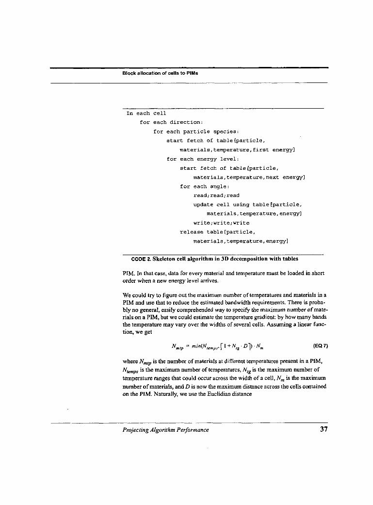
The tables will probably be indexed by particle species, material, temperature, and energy level and give information on particle absorption and scattering. For a time step, the temperature and material will remain constant at a cell, but the waves in each direction will bring values for each particle species and energy level along each angle along that direction. The flow of data into and out of a cell is pictured in Figure 13 on page 36. We can organize the waves to minimize the table fetches from off-chip memory as shown in Code 2 on page 37. We put the loops to handle particle species and energy levels outside the loop for angles. Once we have loaded the table data, we use it for several angles. The streams of data flowing into a cell are shown in Figure 14 on page 36. It is approximately the same for an entire PIM.
The code is written to start prefetches of table data needed next and to release data when it is no longer needed. The underlying assumption is that the table fetches are managed by a software component (e.g. a storage proxy object) that can fetch table elements concurrently with program execution, keep track of how long they are in use, and discard them when they are no longer needed. This fetch-and-release mechanism allows the adjacent cells in a PIM to share the costs of fetching data from the table: they are more likely to have the same temperature and materials than cells far apart, so they are likely to need the same table elements. This is a case where allocating approximately cubic clusters of cells to a PIM is better than just using, for example, row-major order. Not only will their off-chip communications
4. Ron Brightwell, Sandia, personal communication.
Projecting Algorithm Performance 35

FIGURE 13. Data flow into and out of a cell.
Angle A
0 Table (0" 0
FIGURE 14. Flow of data and table elements into a cell.
costs be smaller because of their smaller surface to volume ratio, but with a smaller average distance between the cells, they will be processing fewer different energy levels at the same time and are more likely to contain the same materials at the same temperature. Since the table is indexed by energy levels, materials, and tem- peratures, fewer different table elements should be needed.
It is a problem, though, to estimate the number of table elements that will be loaded. The worst case is that every material is present at every temperature in the
36 Projecting Algorithm Perjbrmance
Block allocation of cells to PlMs
In each cell for each direction:
for each particle species: start fetch of tablerparticle,
materials,temperature,first energy]
for each energy level:
start fetch of tablelparticle, materials,temperature,next energy]
for each angle: read; read;read
update cell using tablerparticle, materials,temperature,energyl
write;write;write
release table [particle,
materials,temperature,energyl
CODE 2. Skeleton cell algorithm in 3D decomposition with tables
PIM. In that case, data for every material and temperature must be loaded in short order when a new energy level amves.
We could try to figure out the maximum number of temperatures and materials in a PIM and use that to reduce the estimated bandwidth requirements. There is proba- bly no general, easily comprehended way to specify the maximum number of mate- rials on a PIM, but we could estimate the temperature gradient: by how many bands the temperature may vary over the widths of several cells. Assuming a linear func- tion, we get
where Nmrp is the number of materials at different temperatures present in a PIM, Nremps is the maximum number of temperatures, Nrg is the maximum number of temperature ranges that could occur across the width of a cell, N , is the maximum number of materials, and D is now the maximum distance across the cells contained on the PIM. Naturally, we use the Euclidian distance
Projecting Algorithm Perjiormance 37

So the time required to load the table elements per cell update is
where S, is the size of a table element, Nu is the number of angles, and Bmem is the memory bandwidth. During every Nu cell updates, we will need to load N m l p . St,
bytes of table space.
33. So, what is the time to process a cell? Cells in a PIM can be processed in parallel. The communications run in parallel with the next cell updates. The table elements can be prefetched in parallel with other processing. A cell cannot be processed faster than any of these parallel opera- tions, so Tcel,, the time to update a cell is
where Tcpu is now the processor time to update a cell. Assuming there is one pro-
cessor assigned to each cell, this will be(cellcycles)/(MIfS x IO6) where cellcycles is the number of processor instruction cycles required to update a cell and MIPS is the number of millions of instructions per second the processor executes.
34. What ifwe send blocks of angles in the same message, as in the KBA algorithm ?
If we pack KUngla values together in a message, then the messages will be longer, but the latencies will only have to be paid once every Kungla steps. This changes the contribution of communication to cell update time to
38 Projecting Algorithm Peflormance

Block allocation of cells to PlMs
35. What if more cells will f i t than there are processors? If there are more cells on a PIM than it has processors, we can share the processors among them taking
cellcycles
M I P S . 10 . m i n ( l , N,,,,,/N) 6
Or, we can just limit the number of cells to the number of processors so as not to slow the processing rate. Or we can allocate as many cells to a PIM as will fit and which do not increase the processing time. This assumes that the communications time or the table access time is the bottle neck. More cells on a PIM will reduce the overall size of machine required to run the program, and as we will see later, that is a significant factor.
36. Aren Y we wasting space trying to have nearly cubic blocks? We do lose some potential cells when we try to allocate rectangular solid blocks. Figure 15 on page 40 shows the number of cells that fit and the communications width for one through 100 cells per PIM. We chose N,, Ny and N, such that
m a x t ~ 3 ~ j - 1, i )sN,s rm1 N x S N y < [ p x l + 1
In Figure 5 on page 0, the x axis indicates the number of cells there is space for on the PIM. The-thick line indicates the number that actually would be placed on the PIM using block allocation. The thin line near the thick one indicates the com- munications width, the number of communications across the three faces to down- stream PIMs. The overlapping thin lines along the bottom show the values of N,, Nv and N,.
Pmjecting Algorithm Performance 39

150
100
50
0
Block allocation
1 9 17 25 33 41 49 57 65 73 81 89 97 Number of cells
- NX Ny NZ - NxA2+NyA2+NzA2 -N
FIGURE 15. Number of cells per block and communication width, block allocation.
Row-major allocation of cells to PlMs
37. What about putting.lully as many cells on a PIM as will fit?
The easiest way to allocate cells is row major order, just like the elements of a mul- tidimensional array. The PlMs are listed in whatever order one wants. The cells are listed along rows in the Z dimension, each successive row after the previous, a plane at a time. If each PIM can hold N cells, then N cells at a time are taken from the cell list and placed in the next PIM in the PIM list. For an Xx Y x 2 array of cells, the number of PIMs required is r ( X x Yx Z ) / N 1 .
40 Projecting Algorithm Performance

Row-major allocation of cells to PlMs
38. What would the communication requirements be with row-major allocation?
If all N cells in a PIM are in the same row, each will have two neighbors on the same PIM, except for the first and the last, but each cell will have four neighbors off-PIM. For any particular sweep, a cell will send messages to only three neigh- bors.
There are a number of cases to consider when analyzing PIM to PIM communica- tion. Firstly, if N evenly divides 2, the N cells in one PIM will communicate with N cells in two other PIMs and the one cell at the end will send a value to the next PIM along the row. Three messages will be sent containing 2 N + 1 values among them.
Secondly, if N does not divide 2, the cells in one PIM may not align with cells in other PIMs. Moreover, some PIMs will contain cells at the end of one row and the beginning of another. Consider the simple case of N cells on a PIM being contigu- ous cells in one row. Since the cells may not be aligned with the cells in other PIMs, the neighboring cells in one direction may be in two different PIMs, so there may be up to five messages sent. In the case that a PIM contains cells from two different rows, each of those blocks of cells may have neighbors in two different PIMs in each direction, giving nine messages that must be sent. There is also a risk that the system might deadlock.
39. How might the system deadlock? Suppose a PIM contains parts of two rows, the end of one and the beginning of
another. On some sweeps, the cells in one of these parts will be down stream of the cells in the other. The cells in one part of the PIM may be waiting for messages to be sent from the cells in the other part of the PIM to intermediary PIMs, but these messages may not be sent until messages from the intermediary PIMs have been received. The easiest way to avoid problems is to separate the cells in the two rows into separately synchronized groups and schedule them separately.
40. How would these messages be spread over the PIM links?
Worst case, all the incoming software links or all the outgoing could be assigned to the same PIM link, so that would give
( 2 . N + 1)xbytesPerMsg
bytes traversing the link every time the cells update their contents. Even if the algo- rithm doesn’t send or receive all values over the same hardware link, we still expect
Projecting Algorithm Performance 41

most PIMs to send or receive at least N x bytesPerMsg bytes over one particular link each Tcpu time.
But latency is the main problem. There will be as many latencies as there are mes- sages that must be sent, at least three and as many as nine.
41. Couldn’t we just align all the rows and keep the number of messages at three? Certainly. That is equivalent to the block allocation with Nx=Ny= 1. If N divides Z, there will be no space wasted; otherwise, space for N, . N y . ( r Z / N ] . N - Z) cells will be wasted.
42. Can weput Kangles values for each cell-cell link together in a message?
Yes, with the usual womes about deadlock if the rows are not aligned.
43. What about the time required to fetch table elements from memory? The maximum number of materials at different temperatures in a PIM is
where Nmrp is the number of materials at different temperatures present in a PIM, Ntemps is the maximum number of temperatures, Nrg is the maximum number of temperature ranges that could occur across the width of a cell, N, is the maximum number of materials, and N is the number of cells assigned to the PIM. The number 2 in the formula comes from the fact that the cells contained in the PIM may form parts of two rows.
The time to load table elements per cell update is given in Equation 9 on page 38.
42 Projecting Algorithm Performance

Rod allocation of cells to PlMs
Rod allocation of cells to PIMs
44. Are there any other allocation orders that have lower communication requirements yet still pack more tightly than block allocation?
Suppose we list the cells not in row-major order, but in the order given by a space- filling curve. Cells near to each other along all dimensions will be near each other in the linear order. When we allocate them to PIMs, they should find more than two of their neighbors in the same PIM, bringing the number of off-chip software links closer to those we would get by allocating cubes or rectangular solid blocks to PIMs. If the PIMs are also listed in order along a space-filling curve, the communi- cating PIMs will be closer together, cutting down the number of hardware links the messages must traverse. The dangers are that:
I. this will increase the number of neighboring PIMs and hence the number of messages sent and the sum of the latencies, and
2. this will create cycles in the message flow among PIMs, requiring separate scheduling of cells or blocks of cells within PIMs, as with row-major allocation.
45. What about approximately cubic blocks, but packed?
We can allocate the cells in blocks that are close to cube-sized. Suppose we have an X x Y x Z array of cells and that Ncells fit on a PIM. Choose N, and N,, such that
Partition the X x Y plane on an rX/N,1 x rX/N,,1 grid, giving “rods” along the Z
dimension. This is similar to the 2D partitioning in the KBA algorithm, except that the rod is not assigned to a single processor, but rather to a column of PIMs.
Projecting Algorithm Performance 43

44 Projecting Algorithm Performance
We allocate cell[x,y,z] to PIM[rx,ryrj where
i, = (x)mod(N,)
iy = (y)mod(Ny)
In essence, we take all the cells in a rod, put them into a linear order, and allocate them to PIMs in that order. We put cell[x,y,z/ at index
(2. N, . Ny + i, . Ny f iy)mod(N)
within PIM[rx,ryrj.
The number of PIMs required for this allocation is
46. Can we have a picture of what the blocks look like? Figure 16 on page 45 shows a block. It has a main body that is a rectangular solid and it extends onto parts of planes above and below.
47. Could there be cycles in this? Would t h b require separate scheduling of sub- block? Yes. There can be cycles that pass back and forth among PIMs. Consider the dia- gram in Figure 17 on page 45. The left side shows a top view of a plane containing part of a lower block and part of an upper block. The wave is flowing in from the upper block into the lower block and in a southeasterly direction along the plane. The right side shows the communication pattern. We are assuming that both the upper and lower blocks have a “main body” consisting of at least one full plane of cells. The main body of the upper block passes values to all the cells in regions L 1, L2, and L3 of the lower block, but the upper block must wait for values to be passed from LI before it can update the cells it has in regions U1, U2, and U3. Sim-

Rod allocation of cells to PlMs
NY
A
FIGURE 16. Block allocated to PIM in rod.
. \4 wave
a I
L1
- - L2
'. Main body of upper
\
FIGURE 17. Communication cycles.
ilarly, L3 must wait on a value to be passed from U1, and U3 must wait for values from L3. There are two communications flowing up-stream, marked a and c. A sin- gle value is passed in a down stream communication, b, from U1 to L3 (although b can be combined with the values U 1 is passing to the main body of the lower block. Each of these blocks can be scheduled separately and can communicate separately. It is also possible for L1 and L2 to be combined into one block, or L2 and L3; also, U1 and U2 may be combined, or U2 and U3, but the blocks connected by a cycle that passes between PIMs cannot be combined. L1 must be scheduled separately from L3, U1 from U3, the main body of the upper block from all of U1, U2, and U3, and all of L1, L2, and L3 separately from the main body of the lower block.
Projecting Algorithm Performance 45

For some other flow directions, there will not be cycles. Suppose the flow was from upper to lower and in a southwesterly direction. All the flow would be from upper into lower blocks.
48. What would the communication bandwidth requirements be for the rod allocation ?
The number of cells exposed along the side of a PIM, i.e. the number of cells adja- cent to cells in a neighboring PIM, will vary. Figure 16 on page 45 gives a sketch of a block allocated to a PIM. The bottom and top, in this figure, contain partial planes, which means that the rest of the plane is contained in the next PIM.
The maximum exposure (maximum number of communicating cells) along a YZ plane is
N y . N, + min(N,,, (N)mod(N, . N,))
where
Notice that Nz is the height of the block of planes full of cells. The actual block may occupy portions of two other planes.
The maximum exposure along a XZ plane is
The maximum exposure along an XY plane depends on the direction the wave is flowing and on the precise number of values on the partial planes. The greatest number of values are exposed when the partial plane has more than N,, values, but not a multiple of N, Consider the partial planes shown in Figure 18 on page 47. We already considered the number of messages and values that need to be communi- cated when the wave is flowing from above to below (U to L) in a south-easterly direction. In counting the number of latencies and number of values sent, we count a block as a lower block on one side, and an upper block on the other, so the num- ber of messages and the number of values that must be sent are all those that must be sent in both directions in looking at one plane.
46 Projecting Algorithm Performance

Rod allocation of cells to PlMs
wave <
2 e
FIGURE 18. Four wave directions through a partial plane.
TABLE 2. Latencies and number of values sent, rod composition.
Wave Direction Latencies Number of values sent
N, x Ny + N, + 1
N x x N y + N y + l
N,x Ny + Ny + 1
N x x N y + N,,+ I
SE 5
NE 3
sw 1
3 N W
Table 2 on page 47 gives the number of latencies and the number of values sent by waves travelling from the upper to the lower blocks along each direction. (Lower to upper would give us the same values, albeit in different directions.) The only differ- ence among the directions is the number of messages that must be sent and hence the number of latencies. In all cases, the number of values that must be sent are N, x Ny + Ny + 1 . The N, x N,, counts the neighboring cells below those on the bot-
tom (i.e. straight down stream). The Ny + 1 counts those beside them. As men- tioned, it is possible to determine more precise, smaller values for these exposures for some relationships of N, N', and N,, for example, when the rod allocation is the same as a block allocation (i.e. when N = N, x N , x N z ) , but since we are interested
Projecting Algorithm Pejbrmance 47

in a bound, we will use five latencies and N , x Ny + Ny + 1 values. Even then, the five latencies can only be achieved with some difficult coding.
49. So what is the communication time for the rod decomposition?
There are several ways we could handle the communications:
I. handle each cell's communications with its neighbors separately, 2. try to batch all the communications from a separately-scheduled block going to
a specific PIM and send them once per update of local cells, 3. stream the data going to a specific PIM much like TCPAP.
Option (1) is too expensive. Option (3) is difficult to analyze, since we would not know the number of messages actually to be sent. We will assume option (2), that all the data passed by a separately scheduled block to a particular neighbor each update cycle are passed in a single message.
Assuming all the communications use the same link, the maximum time required by the bandwidth to get all the bytes in or out is
Assuming as a worst case that all communications have to go in or out one link. The time it takes a message to reach another PIM might be as much as,
since all the communications may be using the same link. An XZ or YZ "face" of exposed cells may be destined to two different PIMs, which accounts for four mes- sages, and the XY faces may need five messages.
48 Projecting Algorithm Performance

Overall cell update time
For simplification, we will make two other assumptions:
1. Kangles will be one; otherwise the program would encounter significantly longer delays around the cycles.
2. Message passing will not run in parallel with cell processing, since the cycles impose blocking and delay. The sum of TcPu and T,,,, is a bound on cell.
50. What is the time required to access DRAM memoiy?
For rod allocation we use Equation 7 on page 37 and Equation 9 on page 38, but we replace Equation 8 on page 38 with
D = [ , / $ + A $ + ( N , + 2 ) 2 ]
Overall cell update time
51. What will the overall cell update time, Tcell, be with the various 3 0 decomposition? The cells in a PIM cannot be updated faster than the communication system can deliver the next values in the streams. While the time to update a cell in block decomposition is
and the lower bound on the cell update time with TOW major order decomposition is
Projecting Algorithm Performance 49

the time to update a cell in rod decomposition is
52. Now that we have the elements, what will be the runtime of a 3 0 decomposition on BGK? We will consider that in the section “Comparing to SMP Clusters” on page 57.
Fault Recovery
53. These applications run for months. There 5 a good chance at least one node will fail during that time. What about check-pointing and recovering from component failure?
The basic idea of check pointing and recovery is that every so often, after a “quan- tum” of work, the state of the cells is saved creating a “snapshot” of the system at that time. When a component fails, the a new component is allocated, the cells are restored from their previous state, and the computation is restarted from there. (This is called “memoization” in other programming contexts.)
The run time is now increased by two components. First, the program spends time creating snapshots. The more often they are made, the slower the program will run. Secondly, when a failure occurs, the state of the computation must be restored from a snapshot and the computation run from there, repeating some computations that have already been performed. The larger the quantum between snapshots, the more time that must be spent repeating computations. The formula for run time now becomes:
T = runtime + timeSavingSnapshots + timeRecoveringFromFailures
To fill in this formula, let
50 Projecting Algorithm Performance

Fault Recovery
T be the overall computation time including taking snapshots and recovering from failures R be the basic run time including neither snapshots nor error recovery
Q be the work “quantum,” the time between snapshots
S be the time to take a snapshot for later recovery, also assumed to be the time to restore and restart the computation after a failure
f be the failure rate, 1 / M T B F , the reciprocal of the mean time between failures, and U be the average time to roll back and recompute after a failure.
The formula for run time becomes
where
(EQ I O )
(EQ 11)
The f. T is the number of failures expected over the duration of the run. The defini- tion of U, the recovery time, is based on the cost of restoring the state of the compu- tation. U is the sum of
1. the time to restore data from a snapshot, assumed to be the same as the time to take a snapshot, since the data merely moves the other direction, although this ignores the costs of allocating a new PIM, and
2. half the time between completing two successive snapshots. If a failure occurs anytime before a quantum is done and the following snapshot is completed, the quantum and snapshot have to be restarted. The expected recomputation time is one half of that period.
The definition of U is not perfect. It does not give a discount for a failure occurring while restoring the state at the beginning of a previous recovery. That would lose only an expected S / 2 , but the probability two failures so close together is low enough that it doesn’t seem worth making U more precis‘e. Nevertheless, we do use
Projecting Algorithm Performance 51

f. T rather than f. (R + LR/Q J . S) to count the probability that a failure might occur sometime during the recovery from a previous failure. This gives
The formula warns that if we use too large a quantum, so that S + (Q + S)/2 approaches the mean time between failure, /. (S+ (Q + S)/2) will approach one, and the run time will grow exponentially.
54. How long will it take to save a snapshot?
If we keep cells totally within a PIM’s on-chip memory, we do not need to resort to disk storage. There is more than enough attached DRAM memory for snapshots. Let’s suppose a PIM saves a snapshot to it’s own DRAM and to the DRAM of some other PIM. We have
S = 2 . N . Scel/Bmem + 2 . N . Scell/Bcomm (EQ 12)
With 6.4MB of PIM memory to save and both memory and communication band- width of 4GB/s, moving the bytes will take at most (6.4/4000) x 4 or 0.0064 sec- onds. The factor 4 counts: (a) one for storing in local DRAM, (b) one for sending to another PIM, and (c) two for receiving from another PIM and storing in local mem- ory. The receiving and storing operations in (3) can be overlapped, reducing the overall factor to closer to three. Counting the software cost, it is still under a sec- ond.
2D Decompositions on PIMs
55. What ifPIMs are not numerous enough to keep the entire array of cells on PIM chips?
The lack of PIMs would be analogous to the lack of processors that motivated the 2D decomposition. We should consider how that could be adapted to PIMs.
52 Projecting Algorithm Pegormance

- ~~~~ ~
2D Decompositions on PlMs
. 1
56. So, how would a KBA-like 2 0 decomposition run on PIMs such as BG/C?
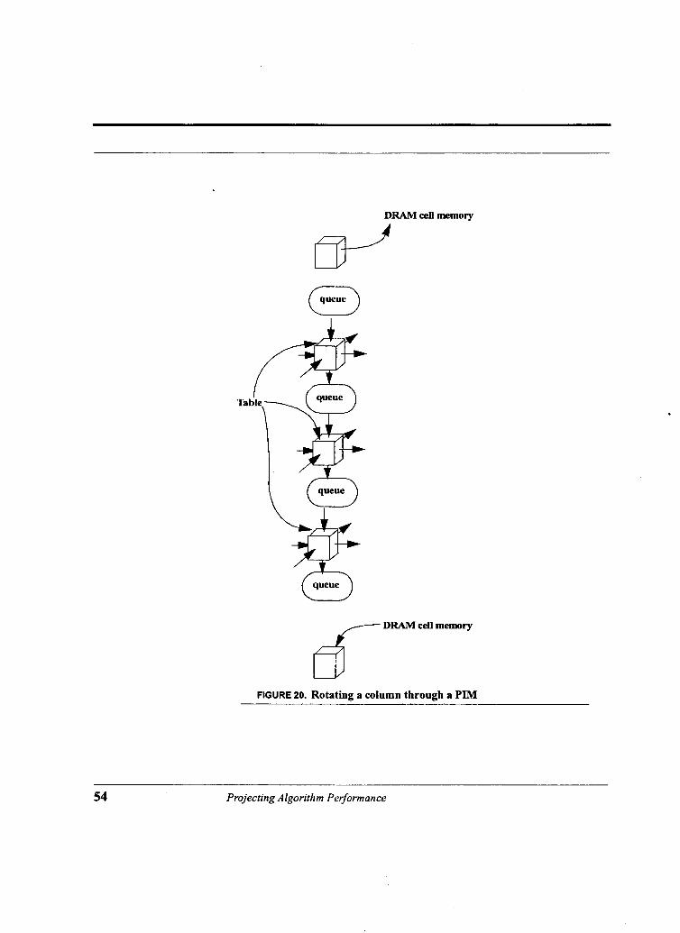
Suppose the X x Y x Z array of cells is placed on a X x Y array of PIMs. The Z cells assigned to a PIM can be kept in DRAM and swapped in and out as necessary. The general data flow for a cell will be that shown in Figure 19 on page 53: Conceptu- ally, the cell goes through a cycle, loading its local cell data from DRAM, loading absorption and scattering data from the table in DRAM as needed, reading and writing values from and to neighboring cells, and finaIly writing its local cell data back into DRAM. Since the data in cell storage can be expected to be much larger than the data being passed among cells, memory bandwidth can be expected to be the main bottleneck in this decomposition. The major effort must be to process as many particle species, angles, and energy levels as possible while the cell’s storage is in the PIM.
4 I -
7 DRAM cell storage
FIGURE 19. Data flow into and out of a cell, 2D on a PIM.
An approach is shown in Figure 20 on page 54. A contiguous segment of a column of cells occupies the PIM at any time. If the PIM can hold N,, cells, at most N,,,, - 1 will be active: The PIM will be loading the next cell down the column and storing the one furthest back.
While it is on the PIM, a cell will read and process all the data for one wave direc- tion, i.e. for all particle species, angles, and energy levels. It will read and write the data being passed in the X and Y dimensions from and to neighboring PIMs. The data along the Z dimension it will read and write from and to on-PIM queues. The most down-stream cell on a PIM will be writing its output to a queue that the next cell loaded will read when it becomes active.
Projecting Algorithm Performance 53
DRAM cell memory
queue c>
queue U
FIGURE 20. Rotating a column through a PIM
54 Projecting Algorithm Performance

rl
f
2D Decompositions on PlMs
57. It appears that the loading and storing of cells would be a huge expense. Is that the bottleneck?
Actually, the data in a cell is proportional to the width of a wave. It has array ele- ments for each angle, energy level, and species of particle. It may require several times as many floating point values for each, but still, it can be viewed as a separate stream flowing into and out of the cell of the same length as the others, but with perhaps a different bandwidth.
A problem, though, is that this swapping stream does not flow in parallel to the other streams, but must flow entirely in before the other streams start and entirely out after they have passed through. The practical effect is that there are fewer pro- cessors updating cells. The memory of at least one will be occupied by a cell that is being stored or a cell that is being loaded. We can model this by setting N, the num- ber of cells per PIM, to
where Scel, is the number of bytes in a cell and Nmap is the number of cells being concurrently loaded or stored.
58. What are the "otherdata " referred to?
There needs to be space for the queues of values being passed along the column. They will contain a total of W values, where W = N, . N e . N, is the number of angles times the number of energy levels times the number of particle species.
The space for the cached table elements is more of a question-several cells that share the same temperature and materials can share the same table elements. We will need
'prbl = Nmip Ns 'te
Projecting Algorithm Performance 55

bytes, where NmIp is defined in Equation 7 on page 37 (but with D=N) and SI, is the size of a table element. If there is an upper bound, N,, on the number of temper- atures over a range of Nconsecutive cells, then we can use that giving:
59. What about fault recovery on a 2D decomposition?
If the DRAM attached to a PIM has space for three columns of cells, we can save snapshots to PIM memory. The formula for S, the time to save the data (see Equa- tion 10 on page 51 and Equation l l on page 51) becomes
S =
where Z is the number of cells along the dimension assigned to the PIM, Sce,l is the number of bytes per cell. The factor 3 counts one for loading a copy of the column which will be both stored locally and transmitted, one for storing it, and one for storing the copy of the column received. The factor 2 counts the cost of sending the column and receiving another. (In practice, the factor may be one, since the trans- mission and reception may use different links. On the other hand, we are not count- ing contention on the links, which could make it worse than two.) For the BG/C, we get
S = 5 . Z . SCel1/(4x1O9)
since both the memory and communication bandwidths are 4 ~ 1 0 ~ .
56 Projecting Algorithm Performance

Comparing to SMP Clusters
60. So what do we expect the run-time on B G K to be with a 2D decomposition?
We would expect it to run more poorly than the 3D row major decomposition. It needs to swap cells into and out of on-PIM storage, which makes the 2D decompo- sition almost certain to be DRAM memory bandwidth bound.
61. Is the 2 0 decomposition worth considering? It may be when we consider applications that are too large to fit in on-chip PIM memory of our machine.
Comparing to SMP Clusters
62. How well do the PIA4 algorithms compare to the SMP clusters? We compared the rod and row-major 3D PIM algorithms to two versions of the KBA algorithm, differing only in whether it was using blocking message passing (TrRpt2dKBA) or non-blocking (TrRpt2dSMP). The problem parameters are shown in Table 3 on page 57. The PIM-specific parameters were taken from the
TABLE 3. Parameters for problem
value 256
256
256
100
12 1
2
20
12
64
100
8
Name X Y Z Na Ne Ns Kangles Ntemps Nits Ntimesteps Nm Smsg
Meaning Dimensions of space
Number of angles per octant Number of energy levels Number of particle species Blocking factor, groups of angles Number of temperature ranges Number of iterations to convergence Number of time steps Max number of materials Size of a datum in a message, in bytes
Pmjecting Algorithm Pe$ormance 57

TABLE 3. Parameters for problem
value Name Meaning 8 Ste Size of a table element, in bytes 16 scv Cell size per angle*energy*species 64 sco Cell size overhead 1 N$ Temperature gradient, how many temperature ranges per
cell width Blue GeneKyclops as presented in Table 1 on page 1 1. We assumed that a cell update took 3 10 cell cycles as taken from a run of SWEEP3D on a PC. (It is proba- bly too high, since the PC result included cache misses, but the PIM algorithm will be running in on-chip memory.)
We use two different algorithm designs for SMP clusters. We use the Hoisie, et al., formulas one of them. For the other, we modify the formulas to assume non-block- ing message passing.
Both use the cell update time for calculating the block update time. The preferred mode of comparison is to feed in actual cell-update figures for the cluster. There is, however, an option to allow the spreadsheet to estimate the performance of an SMP cluster for the problem from processor speed, memory and communication band- width, message-passing latency, etc. This calculation makes the assumption that the cells and table elements are too large to remain in cache memory and hence will have to be reloaded each time through the block of cells being updated. Although comparison with published results indicate that the calculation does not yield utterly preposterous results, nonetheless it should be viewed with suspicion.
The SMP-specific parameters are shown in Table 4 on page 58 and the parameters specific to mapping the algorithm onto the SMP in Table 5 on page 59 By omitting TcpuSMP, we allow the spreadsheet to calculate a block-update time. .
TABLE 4. SMP-specific parameters
value Name Meaning 6.66EM8 Bcomm Communications bandwidth for S W , bytes per sec. 6.66E+08 Bmem Memory bandwidth per processor, bytes per sec. 2.1 OE-05 Tlatency Latency of a message, secs 3.33EM2 MIPS Single Processor: Millions of instructions per second 3.20E+10 Nmem Number of bytes of memory on the SMP
58 Projecting Algorithm Performance

r
. Comparing to SMP Clusters
i
-5
TABLE 4. SMP-specific parameters
16 Nprocs Number of processors per S M P
4096 NmachinePUnits Number of SMPs in representative system
TABLE 5. Mapping-specific SMP parameters.
value Name Meaning (omitted) TcpuSMP Compute time for a cell update. Define TcpuSMP
only to suppress calculation from cellcycles and memory bandwidth. Leave TcpuSMP blank to compute a time bound from cellcycles and mem- ory accesses.
310 cellcycles Number of processor instructions per cell update, not counting data fetches from DRAM.
1 Cache miss rate (needs to be modified for specific problem sizes)
4 Kx Blocking along X axis, Kx x Ky x Z per process
CacheMiss
4 KY 4 K
Blocking along Y axis Blocking along Z
4 PXSMP Processes in X direction per SMP 4 Pysm Processes in Y direction per SMP
TABLE 6. Assumed chip costs and parameters for a representative system.
value Meaning $150.00 costDIMM $300.00 costMPU $300.00 costRouter $500.00 costPIM 500 MB/DIMM 5 Years lifetime of chips
TABLE 7. PIM-specific parameters
Meaning 4.00Ei-09 Bcomm Communications bandwidth, Bytes per sec., one link 4.00E+09 Bmem Memory bandwidth, Bytes per sec. 2.1 OE-05 Tlatency Latency of a message
Projecting Algorithm Performance 59

TABLE 7. PIM-specific parameters
5.00E+02 MIPS Processor: Millions of instructions per second 6.4OEi-06 Nmem Number of bytes of memory on the PIM 1.OOE+O3 MBDRAM Number of megabytes of DRAMRIM 100 Nprocs Number of processors per PIM 262144 NmachinePUnits Number of PIMs in machine
We compared costs of the chips in the minimal machines that could solve the prob- lem. The chip prices we assumed are shown in Table 6 on page 59. This gave the relative costs of the minimal machines to solve the problems (consistent with the parameters) shown in Figure 2 1 on page 60.
.. .. swmm W,an*rwq pIUl3am PIw%rmwqw W m d i
FIGURE 21. Cost of chips in minimal system to solve the problem
The time to solution for the four algorithms are shown in Figure 22 on page 61. The PIM solutions run much faster. When we evaluated the cost-effectiveness of the solutions, we got the costs shown in Figure 23 on page 61.
We then changed the number of angles per octant from 100 to 6 which gave the times to solution shown in Figure 24 on page 62 and the costs shown in Figure 25 on page 62.
60 Projecting Algorithm Performance
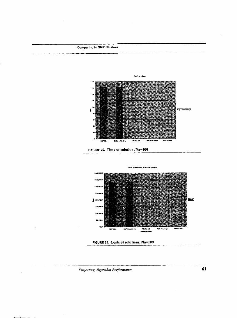
c
.b
Comparing to SMP Clusters
FIGURE 22. Time to solution, Na=100
FIGURE 23. Costs of solutions, Na=100
Projecting Algorithm Performance 61

c
c suPIxB* SLPlnabbanp FlUMad PWN3d.- R W b l D c k
FIGURE 24. Time to solution, Na=6
FIGURE 25. Solution costs, Na=6
62 Projecting Algorithm Performance

Conclusions
There can be two reasons for the change in ratios of cost-effectiveness. First, as shown in Figure 14 on page 36, the PIMs can pre-fetch table elements, but with fewer angles coming in, there is less time to fetch table elements before needing them, so the memory bandwidth for table loads can become the bottleneck. Another explanation is that with more angles, the cell size is larger and the cost of loading all the cells into cache in the SMPs is larger. This means we should carefully check our analysis of SMP solutions to be sure that our assumptions about cache behavior are realistic. We would not want these comparisons to be just an artifact of our assumptions.
Conclusions
63. What have we learned from this work? Particle transport codes can be expected to run as cost-effectively on PIMs as on MPPs and SMP clusters, and potentially vastly more cost-effectively; however, the hardware costs of such systems may be much higher. The PIM-based solutions owe their cost-effectiveness to their greater speed, which they achieve by applying many more processors to the problem. Holding on to the more-expensive hardware for a shorter time can result in improved cost-effectiveness.
The PIM/3D solutions can count on concurrency and the predictability of data accesses to prefetch table elements. This has several consequences:
Latency is reduced or removed relative to demand-paging. The concurrency of PIMs reduces the cell update time to the maximum of pro- cessing, communications, and table-fetch times. (That is, the row-major and block decompositions do.)
If the PIM is communications bound, it is saturating a link. If a link is saturated, other communications across the link add directly to the PIM's processing time. The ability to saturate links makes node allocation and placement more important.
64. What can we say about the strengths and weaknesses of PIMs?
The major advantages of PIMs are the abundance of processors and the low latency to on-chip memory. Unfortunately, the on-chip memory is small and the per-proces-
Projecting Algorithm Performance 63

sor bandwidth of off-chip memory is low. Algorithms that need large tables or code will have difficulty fitting into PIMs.
With radiation transport, we can predict the data needed and pre fetch data from the DRAMS. Since abundant concurrency is available, data can be fetched in parallel with processing. The cost of fetching table elements from DRAM is not added to the time for cell update, but simply forms a lower bound for it.
The concurrency available on PIMs is a major advantage. As long as there are no more cells on a PIM than the number of processors, they can all be updated simulta- neously, along with the communications and memory fetches.
65. Is node allocation really a serious problem? In our spreadsheets we had to assume, worst case, that all communications were routed through the same link, since node allocation would not guarantee that the different neighbors would be accessible via different links.
If node allocation would guarantee virtual links to separate neighbors would go through separate hardware links, then with the exception of rod allocation, the per- formance would be that shown in Figure 26 on page 65. There is a noticeable, albeit not huge difference on performance, and this does not consider the effects of local- ity on latency and effective bandwidth. Since rod allocation passes more messages per cycle than there are links, we had to distribute them in a reasonable fashion.
.
PIM algorithms that use block and row-major allocation are perhaps more suscepti- ble to defects in node allocation than SMP algorithms, since the concurrency on PIMs means that when they are communications bound, they are saturating a link. Any other communications on that link will add time directly to the run-time of the algorithm. PIM-based systems will make schedulers and their node allocators even more important than they are in SMP clusters.
Further work
66. What more needs to be investigated? We need to answer questions such as
64 Projecting Algorithm Performance

Further work
FIGURE 26. Ratios, N a 4 , routing through separate links
What is a good balance between memory and processors on a PIM? What is a good balance between communication bandwidth and DRAM memory band- width? We need to convert the analyses from spreadsheet-based to functions or objects in a programming language to allow programs to search for balance fac- tors. We need to make our analyses, spreadsheets and code available to other researchers, particularly PIM designers. What about wafer-scale integration? The regularity and redundancy of PIMs would allow flawed memory to be masked out, perhaps flawed processors as well. How well could wafer scale integration PIMs run radiation transport? What are the best balance factors? How can radiation transport algorithms to handle larger mesh sizes than can be contained in the PIMs. The PIM 2D allocation is one possibility, but we need to consider the 3D versions as well. How well would other PIM designs work? We’need to explore especially those that have a different balance of parameters. How should nodes be allocated on large meshes of PIMs? There is a good
chance that links are going to be saturated. We need to compare node allocation strategies using queueing theory and our simulation systems to both search for a sound allocation strategy.
Projecting Algorithm Performance 65
What parameters should we be using in our modeling? There is a huge parame- ter space. We need to be refining our models. How well would other algorithms run on PIMs? We need to analyze other important algorithms. What are the software implications of PIMs? Clearly they are not compatible with direct addressing of large address spaces. They place a high premium on concurrency, but at lower than the process-level, and maybe higher than the thread level.
Formulae The formulae for the performance that 3-D allocations share are shown in Box 1 on page 67. The formulae for block allocation are shown in Box 2 on page 68, row- major allocation in Box 3 on page 68, and rod allocation in Box 4 on page 69.
The OverallTime includes checkpointing the program and recovering, as was dis- cussed in the section “Fault Recovery” on page SO.. The checkpoint snapshots are taken every Ksnapsh0& timesteps. R is the run time without snapshots or recovery. T
is the time for one iteration. The formulae for Pomp and POmm were derived over a number of pages, particularly in “Speculating about 3-D decompositions” on page 24.. Tclbl is the time required at access the DRAM table of data on the behav- ior of materials. The time is the time per single cell update. Although the formula is the same for all the allocation strategies, it depends on Nmp, the maximum number of materials at different temperatures per PIM, which differs for the different allo- cations.
Revisions December 15,2002: Added block decomposition. Made a number of small fixes in formulas and phrasing. March 27,2003: Revised rod decomposition to explain the effects of cycles more clearly and precisely.
66 Projecting Algorithm Performance

Revisions
BOX 1.3D PIM Formulae
OverallTime = R + LR/QJ. S 1 _-. ' ( S + ( Q + W 2 )
TMTBF
R = Ntimesteps X 'timestep
'timestep = Nits' T
Q = Ksnapshors ' Ttimestep
Projecting Algorithm Performance 67

Box 2. Block allocation
worst case:
best case:
Box 3. Row major allocation
worst case: Tccomm - - 9 . Tlalency/Kangles + (2 . N + 1 ) . ( Bcomm
best case: Tccomm = 3 . Tlalency/Kangles + ( 2 . N + 1 ) . (‘smsk‘ Kanglerq camm
(EQ 13)
68 Projecting Algorithm Performance

Revisions
BOX 4. Rod allocation
' x =
'Y =
i, = (x)mod(N,)
iy = (y)mod(Ny)
cell[x,y.z] is placed at index
(z . N, . N y + i, . N , 1 . + i,)mod(N)
within PIM[r,, r,, rJ
Projecting Algorithm Performance 69

References Amato, Nancy M., Ping An, 2000, “Task Scheduling and Parallel Mesh Sweeps in Transport Computations,” Texas A&M University, Department of Computer Sci- ence, Technical Report 00-009.
Baker, Randal S., and Raymond E. Alcouffe, 1997, “Parallel 3-D SN Performance For DantsydMPI on the Cray T3D” Proceedings of the Joint InternationaZ Confer- ence on Mathematical Methods and Supercomputing for Nuclear Applications, Vol- ume 1, Saratoga Springs, NY, October 5-9, American Nuclear Society, Inc.
Baker, Randal S., 1999, Parallel SN Methods for Orthogonal Grids, 16th Interna- tional Conference on Transport Theory, Georgia Institute of Technology.
Hoisie, Adolfy, Olaf Lubeck, Harvey Wasserman, Fabrizio Petrini, Hank Alme, 2000a, “A General Predictive Performance Model for Wavefront Algorithms on Clusters of SMPs,” proceedings of the 2000 International Conference on Parallel Processing (ICPP 2000), IEEE Computer Society.
Hoisie, Adolfy, Olaf Lubeck, and Harvey Wasserman, 2000b, “Performance and Scalability Analysis of Teraflop-Scale Parallel Architectures Using Multidimen- sional Wavefront Applications,” The International Journal of High Performance Computing Applications, Sage Science Press, Volume 14, Number 4.
International Technology Roadmap for Semiconductors: 200 1 Edition. http://pub- lic .i trs .net/Files/200 1 ITRS/Home .htm
Kerbyson, Darren, Adolfy Hoisie, and Harvey Wasserman, 2002, “A Comparison Between the Earth Simulator and Alpha Server Systems Using Predictive Applica- tion Performance Models,” 16 Oct. 2002, LA-UR-02-5222.
Koch, K. R., R. S. Baker, and R. E. Alcouffe, 1992, “Solution of the first-order form of the 3-D discrete ordinates equation on a massively parallel processor,” Transactions of the American Nuclear Society, 65( 108): 198- 199.
Mathis, Mark M., Nancy M. Amato, and Melvin L. Adams, 2000, “A General Per- formance Model for Parallel Sweeps on Orthogonal Grids for Particle Transport Calculations,” 14th ACM International Conference on Supercomputing (ICS’OO), Santa Fe, New Mexico.
70 Projecting Algorithm Performance
i
c-

References
Plimpton, Steve, Bruce Hendrickson, Shawn Burns, Will McLendon 111,2000, “Parallel Algorithms for Radiation Transport on Unstructured Grids,” Proc. sc’oo, IEEE, 0-7803-9802-5/2000.
Vikram Adve, Flowchart & Pipelines for SWEEP 3D, 2002, www.cs.rice.edu/ -adve/sweep3D/.
Sundaram-Stukel, David, Mary K. Vernon, 1999, “Predictive Analysis of a Wave- front Application Using LogGP,” Proceedings of the seventh ACM SIGPLAN sym- posium on Principles and practice of parallel programming, ACM Press, also published in ACMSIGPUNNotices Volume 34, Issue 8 (August 1999).
Vetter, Jeffrey S., Andy Yoo, 2002, “An Empirical Performance Evaluation of Scal- able Scientific Applications,” Proc. SC 2002, IEEE, 0-7695-1 524-X/02.
Projecting Algorithm Performance 71

INTENTIONALLY LEFT BLANK
72 Projecting Algorithm Performance

DISTRIBUTION:
t
1 1 1 1 1 1 1 1 1 1 1 1 1 1 1 1
1 1 1 1 1 1 1 1 1 1 1 1 1 1 1 1 1 1 1 1 1 1 1 1 1 1
73
9019 9012 9012 901 1 9915 9019 9012 9217 0824 0847 0824 0835 0833 0834 0555 0821
0835 0826 0893 1183 0835 0834 0847 1135 0826 0825 0557 0836 0847 0836 0847 0321 0318 0847 03 10 1110 1111 0310 1110 1110 0847 0822
1 MS 9037 J. C. Berry, 8945 S. C. Carpenter, 8945 J. A. Friesen, 8963 S. C. Gray, 8949 B. V. Hess, 8941 M. L. Koszykowski, 8961 B. A. Maxwell, 8945 P. E. Nielan, 8964 S. W. Thomas, 8962 A. C. Ratzel, 91 10 H. S. Morgan, 9120 J. L. Moya, 9130 J. M. McGlaun, 9140 B. J. Hunter, 91 03 M. R. Prarie, 9 1 12 M. S. Garrett, 9122 L. A. Gritzo, 9 132
E. A. Boucheron, 9141 S. N. Kempka, 91 13 J. Pott, 9123 M. W. Pilch, 9133 K. F. Alvin, 9142 J. E. Johannes, 91 14 J. M. Redmond, 9124 S. R. Heffelfinger, 9134 J. D. Zepper, 9143 B. Hassan, 91 15 T. J. Baca, 9125 E. S. Hertel, Jr., 91 16 R. A. May, 9126 R. 0. Griffith, 91 17 J. Jung, 9127 P. R. Graham, 9208 J. E. Nelson, 9209 S. A. Mitchell, 921 1 M. D. Rintoul, 9212 D. E. Womble, 92 14 B. A. Hendrickson, 9215 R. W. Leland, 9220 N. D. Pundit, 9223 D. W. Doerfler, 9224 T. D. Blacker, 9226 P. Heermann, 9227
1 MS 0318 P. Yarrington, 9230 1 1 1 1 1 1 1 1 1 1 1 1 1 1 1 1
1 1 1
1
2
1
0819 0820 03 16 0316 0813 080 1 0806 0822 0807 0805 0812 0813 0812 0809 0806 1110
R. M. Summers, 9231 P. F. Chavez, 9232 S. S. Dosanjh, 9233 J. B. Aidun, 9235 R. M. Cahoon, 931 1 F. W. Mason, 9320 C. Jones, 9322 C . Pavlakos, 9326 J. P. Noe, 9328 W.D. Swartz, 9329 M. R. Sjulin, 9330 A. Maese, 9333 M. J. Benson, 9334 G. E. Connor, 9335 L. Stans, 9336 R. B. Brightwell, 9224
1 1 10 R. E. Riesen, 9223 11 10 K. D. Underwood, 9223 1 110 E. P. DeBenedictis, 9223
90 18 Central Technical Files, 8940-2
0899 Technical Library, 49 16
0612, Review & Approval Desk, 4912, for DOE/OSTI


![A High-Speed 64-Bit Binary Comparator€¦ · A high-speed 64-bit binary comparator 39 | Page III. EXISTING 64-BIT BINARY COMPARATOR DESIGN 64-bit comparator in reference [8], [9],](https://img.pdfslide.us/doc/110x75/5eac1a458d19873e777698b4/a-high-speed-64-bit-binary-comparator-a-high-speed-64-bit-binary-comparator-39-.jpg)