Embed Size (px)
Citation preview

1
Report on Operation of China’s Iron Ore Spot Market
(2017)
In 2017, the iron and steel industry in China was the most characterized by the high
profits at the steel mills and the sustained effect of the production restriction policies
for environmental protection. Since 2017, the steel mills have turned from losses to
profits in production, and remained at the high profit level of about RMB 1,000 per
tonne of steel for a long time. The steel mills are active in production, strongly boosting
the upstream and downstream products on the ferrous industry chain. In addition, the
frequently released and strictly implemented policies for environmental protection,
production restriction, and transportation restriction and so on have had a major impact
on the coal, coke, steel and ore industries.
I. The iron ore prices showed two rounds of up-and-down movements with
fierce fluctuations.
In 2017, the spot prices of iron ore fluctuated significantly. De-capacity and policies
for environmental protection led to tight supply of steel, the profits per tonne of steel
continued to be at high levels, and the steel mills were active in production, resulting in
the shortage of high-grade ore for some time, which bolstered the prices of the upstream
raw materials in the period; However, the total supply of iron ore was always relatively
sufficient with the total inventory at ports remaining at a high level, and starting in the
third quarter of the year, the policies for environmental protection, production

2
restriction and so on saw the enforcement continuously strengthened, causing the steel
mills to carry out overhauls intensively or suspend production with the demand for raw
materials reduced.
(I) The prices of iron ore were highly volatile.
At the end of November, the spot price of iron ore was RMB 531 / tonne, a decrease
of 17.03% from the beginning of the year. Although the price did not record great
changes on the whole, it experienced two rounds of “ups and downs” in the year. The
annual price swing1 was as high as 62.22%, and the annualized daily volatility stood
at 31.27%, with both lower than last year.
Chart 1: Spot Price Trend of Iron Ore
1 swing = (the highest price – the lowest price) / the lowest price
Vehicle-board Price of Newman Fines at Qingdao Port

3
Table 1: Swing and Annualized Daily Volatility of Iron Ore Spot Price
Year Swing of Spot Price Daily Volatility of
Spot Price
2014 89.58% 14.78%
2015 71.67% 20.62%
2016 112.5% 42.96%
Jan to Nov, 2017 62.22% 31.27%
(II) Steel prices have a one-way guiding effect on the changes of the iron ore
prices.
Generally speaking, in the year the supply of iron ore was relatively sufficient. The
main factor affecting the iron ore prices was the demand of the downstream steel
production. With the policy for capacity reduction gradually implemented and the
enforcement strengthened, in May 85% of the planned reduction in crude steel for the
year was completed with the production capacity of the crude steel cut by 42.39 million
tonnes, resulting in a significant impact on the steel production capacity and thus
serving as the dominant factor affecting the upstream and downstream price
fluctuations on the entire steel industry chain.
With the confidence interval at 95%, from January to November 2017, the spot price
of rebar had a one-way guiding effect on the price of iron ore, with the effect growing
stronger.
Table 2: Rebar Spot Price Having a One-way Guiding Effect on Iron Ore Spot Price
Table 3: Guiding Relationship between Spot Prices of Rebar and Iron Ore from 2014
to 2017
Year Null Hypothesis F-statistic Prob Conclusion
2014 Rebar does not Granger cause iron ore 6.49087 0.0018 Rebar and iron ore guide each
other. Iron ore does not Granger cause rebar 5.75081 0.0036
2015 Rebar does not Granger cause iron ore 3.02912 0.0502
Rebar guides iron ore. Iron ore does not Granger cause rebar 0.85077 0.4284
2016 Rebar does not Granger cause iron ore 101.067 1.E-32 Rebar and iron ore guide each
other. Iron ore does not Granger cause rebar 3.43570 0.0338
20172 Rebar does not Granger cause iron ore 57.7561 9.E-21 Rebar guides iron ore.
2 The 2017 data are for the period ending on November 21, 2017.

4
Iron ore does not Granger cause rebar 0.30681 0.7361
(III) Ratio of the prices of rebar to iron ore was at a high level continuously.
According to the historical data, the reasonable range of price ratios for rebar and
iron ore is around 5.5. However, with the supply-side reform deepened in the year, the
rebar prices rose sharply, and the ore prices followed the uptrend but with modest gains.
As a result, the ratio of the prices of rebar to iron ore continued to expand starting in
February of the year, and the ratio of the spot prices of rebar to iron ore hit the record
high of more than 8.0 in late June. Subsequently, although the ore prices stopped falling
and picked up with the ratio restored to some extent in August, the steel prices
continued to rise sharply soon afterwards, with the iron ore prices recording fewer gains
or even some losses, causing the ratio of the spot prices of rebar to iron ore to reach the
new high of 9.32 in early December and leading to the high pressure for the iron ore
prices to catch up with the increases in the future.

5
Chart 2: Price Ratios of Rebar to Iron Ore
II. Operation of Iron Ore Spot Market
(I) The iron ore reported sufficient supply with the inventory at a high level
continuously.
1. The total supply of iron ore increased, with the concentration almost at the same
level as the previous year. According to the estimates of some organization3, in 2017
the total global iron ore supply would increase by 5.85% over the previous year to reach
2.083 billion tonnes. Australia was still the largest supplier of iron ore, with the supply
expected to amount to 900 million tonnes, accounting for 43.24% of the world's total.
The supply concentration for Australia and Brazil was 63.66%, which was basically
unchanged from the last year.
Table 4: Iron Ore Supplies of Different Countries in 2017 (Unit: million tonnes)
Country 2016 2017E Variation
1 Australia 852.6 900.8 48.2
2 Brazil 400.3 432 31.7
3 China 245 270 25
3 Report of Mysteel on Iron Ore Operation in the First Half of 2017
Price: Rebar: HRB400 20mm: Shanghai Vehicle-board Price: Qingdao Port: Australian: Newman
Fines: 62.5% Ratio of Spot Prices of Rebar to Iron Ore
Source of Data: Wind Information
RMB / tonne
RMB / wmt
RMB / tonne
RMB / wmt

6
4 Russia 84 84.3 0.3
5 Canada 71.9 73.6 1.7
6 South Africa 55.6 59.4 3.8
7 Ukraine 42.5 42.3 -0.2
8 India 37.3 40.1 2.8
9 Sweden 26.5 24 -2.5
10 Chile 16.8 16.4 -0.4
Sum 1968 2083.1 115.1
2. The inventories at the ports continued to be at a high level, and structural
shortages of high and low grades of ore caused prices of iron ore to go up in a short
period of time. Starting in the beginning of the year, the iron ore inventories at ports
were at a historically high level, with an average annual inventory of 135 million tonnes,
an increase of 29.64% over the previous year. Although the inventories were at a
relatively high level, the steel mills saw their demands for iron ore of high and low
grades changing with their varying enthusiasm for production. Therefore, different
grades of iron ore might meet with short supply, thus affecting the prices of different
grades of iron ore.
Chart 3: Iron Ore Inventories at Ports
(II) The monopoly of the four major mines was firm, with the space for cost
reduction limited and the output growth slowing down.
1. With the strategic expansion underway, the oligopoly status of the four major
mines was firm. Since 2010 the four major mines have adopted the strategy of low-cost
expansion to further snatch market shares, and the high-cost iron mines including those
数据来源:Wind资讯
国内铁矿石港口库存量
15-04-30 15-07-31 15-10-31 16-01-31 16-04-30 16-07-31 16-10-31 17-01-31 17-04-30 17-07-31 17-10-3115-04-30
8100 8100
9000 9000
9900 9900
10800 10800
11700 11700
12600 12600
13500 13500
14400 14400
万吨 万吨万吨 万吨10,000 tonnes
Iron Ore Inventories at Ports in China
Source of Data: Wind Information
10,000 tonnes

7
in China and the overseas non-mainstream mines have gradually withdrawn from the
market, with the output of the four major mines accounting for 56.8% of the world's
total. The oligopoly pattern has been further consolidated and it is expected that the
ratio would remain at this level in 2017.
Chart 4: Global Supply of Iron Ore
Chart 5: Ratio of Outputs of Four Major Mines to the World
2. The shrinking space for cost reduction at the four major mines bolstered the iron
ore prices. At the current prices, the four major mines had a small profit margin: the
FMG, which mainly produces low-grade iron ore, had a gross profit margin of US$ 11.4
/ tonne; among the three major mines producing high-grade iron ore, the gross profit
margin of Vale was also only US$ 16.6 / tonne. With the costs reduced and efficiency
increases continuously, the costs at the four major mines have been low, and there is
limited room for cost reductions in the future.
0
5
10
15
20
2009 2010 2011 2012 2013 2014 2015 2016 2017
全球产量(亿吨) 四大矿产量(亿吨)
56.8%
56.7%
0%
10%
20%
30%
40%
50%
60%
-1.5
0.0
1.5
3.0
2009 2010 2011 2012 2013 2014 2015 2016 2017
全球产量变化(亿吨) 四大矿产量变化(亿吨)
四大矿产量占比(右轴)
Global Output (100 million tonnes) Output of Four Major Mines (100 million tonnes)
Change of Global Output (100
million tonnes) Change of Output at Four Major Mines
(100 million tonnes) Proportion of Four Major Mines (Right Axis)
8
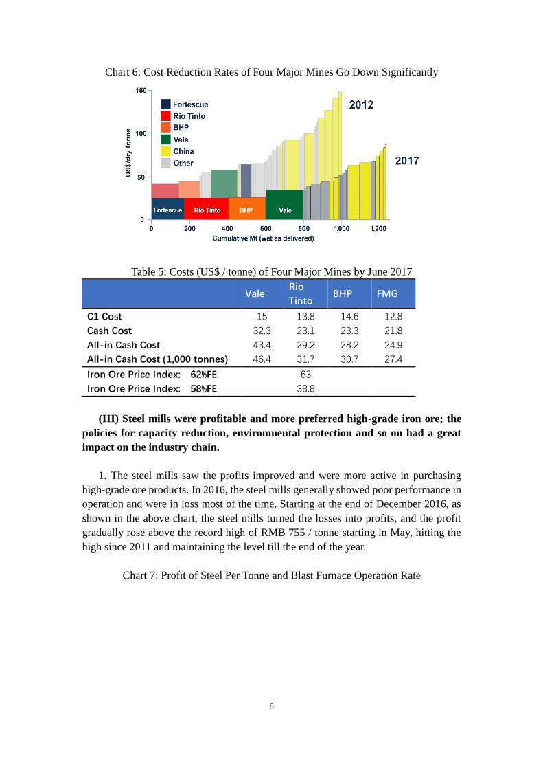
Chart 6: Cost Reduction Rates of Four Major Mines Go Down Significantly
Table 5: Costs (US$ / tonne) of Four Major Mines by June 2017
Vale Rio
Tinto BHP FMG
C1 Cost 15 13.8 14.6 12.8
Cash Cost 32.3 23.1 23.3 21.8
All-in Cash Cost 43.4 29.2 28.2 24.9
All-in Cash Cost (1,000 tonnes) 46.4 31.7 30.7 27.4
Iron Ore Price Index: 62%FE 63
Iron Ore Price Index: 58%FE 38.8
(III) Steel mills were profitable and more preferred high-grade iron ore; the
policies for capacity reduction, environmental protection and so on had a great
impact on the industry chain.
1. The steel mills saw the profits improved and were more active in purchasing
high-grade ore products. In 2016, the steel mills generally showed poor performance in
operation and were in loss most of the time. Starting at the end of December 2016, as
shown in the above chart, the steel mills turned the losses into profits, and the profit
gradually rose above the record high of RMB 755 / tonne starting in May, hitting the
high since 2011 and maintaining the level till the end of the year.
Chart 7: Profit of Steel Per Tonne and Blast Furnace Operation Rate

9
As shown in the above chart, in the year, the steel mills turned the losses into profits,
which continued to be at a high level, and the operation rate kept rising to more than
77%. The steel mills actively procured high-grade ore to increase the rate of tapping
iron, resulting in a structural shortage of high-grade ore. The price difference of high
and low-grade ore (61.5% PB and 58% Yandi) once widened to more than RMB 100 /
wmt. The average price difference of high and low grades of ore stood at US$ 28.8 /
tonne, a year-on-year increase of 108%.
Chart 8: Price Difference between High and Low-grade Iron Ore
2. The policy for dealing with the substandard steel caused the steel scrap to replace
the iron ore to some extent. In 2017, with the enforcement of banning the “substandard
steel” and “intermediate frequency furnaces” and other industrial policies and the
数据来源:Wind资讯
吨钢利润 高炉开工率:全国
17-01-31 17-03-31 17-05-31 17-07-3117-08-31 17-10-3117-01-31
200 200
400 400
600 600
800 800
1000 1000
1200 1200
1400 1400
元/吨 元/吨元/吨 元/吨
64 64
66 66
68 68
70 70
72 72
74 74
76 76
78 78% %% %
051015202530354045
0102030405060708090
100
高低品味价差(右轴) 62%Fe 58%Fe
RMB / tonne RMB / tonne
Profit of Steel per tonne Blast Furnace Operation Rate: Nationwide
Source of Data: Wind Information
Price Difference of High and Low-grade
Ore (Right Axis)

10
strictest policies for environmental protection, the substandard steel was almost
eliminated with the production by the intermediate frequency furnaces basically
suspended, and the steel scrap for raw material was in great surplus by the end of June.
In the first half of the year, the steel scrap prices dropped sharply, thereby reducing the
production cost for electric arc furnaces. The advantage of electric arc furnaces in cost
began to appear, and many converters also started to increase the adoption of scrap steel.
As a result, some demand for iron ore was replaced by steel scrap, putting some
downward pressure on iron ore prices.
Chart 9: Price Trends of Steel, Steel Scrap and Iron Ore
According to the statistics of the Steel Scrap Association, from January to
September in the year, the total consumption of iron and steel scrap was 101.23 million
tonnes, an increase of 36.53 million tonnes or 56.5% year on year. The increase in the
use of steel scrap caused the trends of the iron ore prices and the prices at the steel mills
to differ over a period of time. In May of the year, the prices of steel scrap fell to the
year low, the steel prices went up due to the short supply and the iron ore prices declined
under pressure.
III. Expectation of Market Developments and Changes in the Future
(I) Demand: Demands for real estate and infrastructure construction will slow
down, with the demand of home appliances and vehicles under pressure.
1. The property investment has showed resilience, but it will still be suppressed by
sales decline in the long run. From January to October 2017, the year-on-year growth
RMB / tonne
RMB / tonne
RMB / tonne
Price Including Tax: Steel Scrap
Shanghai
Rebar: HRB400 20mm: Shanghai Vehicle-board Price of Newman Fines: Qingdao Port
(Right Axis)
Source of Data: Wind Information

11
rates of the area for commercial housing sales, the area for land acquisition, the area for
new constructions and the cumulative investment in real estate development were
8.20%, 12.90%, 5.60% and 7.80% respectively. Currently, the property investment
supported by the purchase of land has showed strong resilience. However, if the land
acquisition and price factors were deducted, the year's growth of investment in real
estate development would be negative on a year-on-year basis. Against the backdrop of
“housing for living instead of speculation”, the relatively tight tone of the policy for
real estate will not be changed in the next year, and the demand for real estate will
continue to be depressed by sales decline.
Chart 10 Investment in Real Estate (with Land Purchase Price Factor Deducted) from
2014 to September 2017
2. The investment and financing platforms and PPP will be tightened, and the
growth of the infrastructure construction will slow down. From January to October, the
accumulative total investment in infrastructure construction increased by 15.85%, a
decrease of 0.03 percentage point from the figure for the first 9 months in the year,
showing stable growth in general. The growth rate is estimated at 14.5% in 2018, lower
than that in 2017.
Chart 11: Investment in Infrastructure Construction (with Price Factor Deducted)
from 2014 to September 2017
-10%
-5%
0%
5%
10%
15%
0
5,000
10,000
15,000
20,000
25,000
30,000
2014-0
3
2014-0
6
2014-0
9
2014-1
2
2015-0
3
2015-0
6
2015-0
9
2015-1
2
2016-0
3
2016-0
6
2016-0
9
2016-1
2
2017-0
3
2017-0
6
2017-0
9
房地产开发投资:单季(亿)
房地产开发投资:季同比
Investment in Real Estate Development: Single Quarter (RMB 100 million)
Investment in Real Estate Development: Quarterly Year-on-Year

12
3. The demand of vehicles and home appliances was under pressure. The
automobile purchase tax concession led to a high sales base in 2016. The growth in
sales showed the sluggish sign in 2017, and with the tax concession expiring at the end
of the year, the sales volume is expected to increase by 4% in 2018. As the cycle of the
home appliances industry follows the real estate industry cycle, the home appliances
industry will face pressure in production and sales with the real estate industry to be
suppressed by the long-term decline in sales.
Chart 12: Auto Sales from 2014 to October 2017
Chart 13: Accumulative Production of Home Appliances from 2014 to October 2017
0
10,000
20,000
30,000
40,000
50,000
60,000
0%
5%
10%
15%
20%
25%
30%
2014-0
3
2014-0
6
2014-0
9
2014-1
2
201
5-0
3
2015-0
6
2015-0
9
2015-1
2
2016-0
3
2016-0
6
2016-0
9
201
6-1
2
2017-0
3
2017-0
6
2017-0
9
基建投资:单季(亿) 基建投资:季同比
0%
2%
4%
6%
8%
10%
12%
14%
16%
0
500
1000
1500
2000
2500
3000
2014 2015 2016 2017
汽车销量累计值(万辆) 汽车销量累计同比
Investment in Infrastructure Construction:
Single Quarter (RMB 100 million)
Investment in Infrastructure Construction:
Quarterly Year-on-Year
Accumulative Auto Sales (10,000 Vehicles) Accumulative Auto Sales Growth Year-on-Year
13
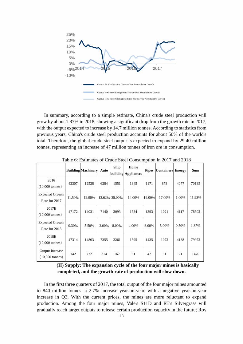
In summary, according to a simple estimate, China's crude steel production will
grow by about 1.87% in 2018, showing a significant drop from the growth rate in 2017,
with the output expected to increase by 14.7 million tonnes. According to statistics from
previous years, China's crude steel production accounts for about 50% of the world's
total. Therefore, the global crude steel output is expected to expand by 29.40 million
tonnes, representing an increase of 47 million tonnes of iron ore in consumption.
Table 6: Estimates of Crude Steel Consumption in 2017 and 2018
Building Machinery Auto Ship
building
Home
Appliances Pipes Containers Energy Sum
2016
(10,000 tonnes) 42307 12528 6284 1551 1345 1171 873 4077 70135
Expected Growth
Rate for 2017 11.50% 12.00% 13.62% 35.00% 14.00% 19.00% 17.00% 1.00% 11.93%
2017E
(10,000 tonnes) 47172 14031 7140 2093 1534 1393 1021 4117 78502
Expected Growth
Rate for 2018 0.30% 5.50% 3.00% 8.00% 4.00% 3.00% 5.00% 0.50% 1.87%
2018E
(10,000 tonnes) 47314 14803 7355 2261 1595 1435 1072 4138 79972
Output Increase
(10,000 tonnes) 142 772 214 167 61 42 51 21 1470
(II) Supply: The expansion cycle of the four major mines is basically
completed, and the growth rate of production will slow down.
In the first three quarters of 2017, the total output of the four major mines amounted
to 840 million tonnes, a 2.7% increase year-on-year, with a negative year-on-year
increase in Q3. With the current prices, the mines are more reluctant to expand
production. Among the four major mines, Vale's S11D and RT's Silvergrass will
gradually reach target outputs to release certain production capacity in the future; Roy
-10%
-5%
0%
5%
10%
15%
20%
25%
2014 2015 2016 2017
产量:空调:累计同比
返回目录产量:家用电冰箱:累计同比
产量:家用洗衣机:累计同比
Output: Air Conditioning: Year-on-Year Accumulative Growth
Output: Household Refrigerator: Year-on-Year Accumulative Growth
Output: Household Washing Machine: Year-on-Year Accumulative Growth

14
Hill has reached full capacity and there is room for growth in the first half of 2018.
There is basically no other new capacity addition. It is estimated that S11D will push
up production by 20 million tonnes in the next year, with the increases of 10 million
tonnes for Silvergrass and 8 million tonnes for Roy Hill, resulting in a total of 38 million
tonnes.
Table 7: 2017 Production and Long-term Capacity Plans of Four Major Mines (Unit:
million tonnes)
17Q1 16Q1 YoY 17Q2 16Q2 YoY 17Q3 16Q3 YoY 17
Q1-3
16
Q1-3 YoY
Long-term
Capacity
Plan
Vale 86.20 77.54 11.2% 91.85 86.82 5.8% 95.11 92.09 3.3% 273.16 256.46 6.5% 400.00
Rio
Tinto 81.56 84.02 -2.9% 84.37 85.27 -1.0% 90.37 88.14 2.5% 256.29 257.42 -0.4% 330.00
BHP 53.58 53.06 1.0% 60.14 55.63 8.1% 55.59 57.59 -3.5% 169.30 166.27 1.8% 252.00
FMG 44.70 43.40 3.0% 53.50 47.80 11.9% 45.70 49.50 -7.7% 143.90 140.70 2.3% 200.00
Total
of the
Four
266.03 258.02 3.1% 289.86 275.51 5.2% 286.76 287.32 -0.2% 842.65 820.85 2.7% 1182.00
(III) It is expected that the demand for crude steel will increase in 2018, and
the production expansion will be limited at the mines.
It is expected that in 2018, the apparent demand for crude steel in the world will
increase by 29.4 million tonnes, equivalent to 47 million tonnes of iron ore. The
expansion cycle of the four major mines has basically come to an end. In 2018, their
production will increase by about 38 million tonnes, with the demand gap at about 9
million tonnes.
Chart 14: Apparent Demand for Crude Steel in the World (Except China) (Unit:
10,000 tonnes / %)

15
-30%
-20%
-10%
0%
10%
20%
30%
0
10,000
20,000
30,000
40,000
50,000
60,000
70,000
80,000
90,000
100,000