Embed Size (px)
Citation preview

D4.15 Report on Numerical Methods for PTO Systems
Page 1 of 45
WP2: Marine Energy System Testing - Standardisation and Best Practice
Deliverable 4.15
Report on Numerical Methods for PTO Systems
Marine Renewables Infrastructure Network
Status: Final Version: 03 Date: 22-Jan-2014

2
ABOUT MARINET MARINET (Marine Renewables Infrastructure Network for emerging Energy Technologies) is an EC-funded network of research centres and organisations that are working together to accelerate the development of marine renewable energy - wave, tidal & offshore-wind. The initiative is funded through the EC's Seventh Framework Programme (FP7) and runs for four years until 2015. The network of 29 partners with 42 specialist marine research facilities is spread across 11 EU countries and 1 International Cooperation Partner Country (Brazil). MARINET offers periods of free-of-charge access to test facilities at a range of world-class research centres. Companies and research groups can avail of this Transnational Access (TA) to test devices at any scale in areas such as wave energy, tidal energy, offshore-wind energy and environmental data or to conduct tests on cross-cutting areas such as power take-off systems, grid integration, materials or moorings. In total, over 700 weeks of access is available to an estimated 300 projects and 800 external users, with at least four calls for access applications over the 4-year initiative. MARINET partners are also working to implement common standards for testing in order to streamline the development process, conducting research to improve testing capabilities across the network, providing training at various facilities in the network in order to enhance personnel expertise and organising industry networking events in order to facilitate partnerships and knowledge exchange. The initiativeconsists of five main Work Package focus areas: Management & Administration, Standardisation & Best Practice, Transnational Access & Networking, Research,and Training& Dissemination. The aimis to streamline the capabilities of test infrastructures in order to enhance their impact and accelerate the commercialisation of marine renewable energy. See www.fp7-marinet.eu for more details.
Partners
Ireland University College Cork, HMRC (UCC_HMRC)
Coordinator
Sustainable Energy Authority of Ireland (SEAI_OEDU)
Denmark Aalborg Universitet (AAU)
DanmarksTekniskeUniversitet (RISOE)
France EcoleCentrale de Nantes (ECN)
InstitutFrançais de Recherche Pour l'Exploitation de la Mer (IFREMER)
United Kingdom National Renewable Energy Centre Ltd. (NAREC)
The University of Exeter (UNEXE)
European Marine Energy Centre Ltd. (EMEC)
University of Strathclyde (UNI_STRATH)
The University of Edinburgh (UEDIN)
Queen’s University Belfast (QUB)
Plymouth University(PU)
Spain Ente Vasco de la Energía (EVE)
Tecnalia Research & Innovation Foundation
(TECNALIA)
Belgium 1-Tech (1_TECH)

3
Netherlands Stichting Tidal Testing Centre (TTC)
StichtingEnergieonderzoek Centrum Nederland (ECNeth)
Germany Fraunhofer-GesellschaftZurFoerderung Der AngewandtenForschung E.V (Fh_IWES)
Gottfried Wilhelm Leibniz Universität Hannover (LUH)
Universitaet Stuttgart (USTUTT)
Portugal Wave Energy Centre – Centro de Energia das Ondas (WavEC)
Italy UniversitàdegliStudidi Firenze (UNIFI-CRIACIV)
UniversitàdegliStudidi Firenze (UNIFI-PIN)
UniversitàdegliStudidellaTuscia (UNI_TUS)
ConsiglioNazionaledelleRicerche (CNR-INSEAN)
Brazil Instituto de PesquisasTecnológicas do Estado de São Paulo S.A. (IPT)
Norway SintefEnergi AS (SINTEF)
NorgesTeknisk-NaturvitenskapeligeUniversitet (NTNU)

0
DOCUMENT INFORMATION Title Report on Numerical Methods for PTO Systems
Distribution Work Package Partners
Document Reference MARINET-D4.15
Deliverable Leader
Sara Armstrong, Darren Mollaghan UCC-HMRC
Contributing Authors
[Type name or delete row] [Choose organisation] [Type name or delete row] [Choose organisation]
REVISION HISTORY Rev
. Date Description Prepared by
(Name & Org.) Approved By (Task/Work-
Package Leader)
Status (Draft/Final)
01 28/12/12 Draft prepared as index for WP4 guidance SA,DM HMRC n/a n/a
02 23/12/13 Draft Deliverable SA,DM, JR n/a n/a
03 1/04/14 Final SA,DM, JR
ACKNOWLEDGEMENT The work described in this publication has received support from the European Community - Research Infrastructure Action under the FP7 “Capacities” Specific Programme through grant agreement number 262552, MaRINET.
LEGAL DISCLAIMER The views expressed, and responsibility for the content of this publication, lie solely with the authors. The European Commission is not liable for any use that may be made of the information contained herein.This work may rely on data from sources external to the MARINET project Consortium. Members of the Consortium do not accept liability for loss or damage suffered by any third party as a result of errors or inaccuracies in such data. The information in this document is provided “as is” and no guarantee or warranty is given that the information is fit for any particular purpose. The user thereof uses the information at its sole risk and neither the European Commission nor any member of the MARINET Consortium is liable for any use that may be made of the information.

1
EXECUTIVE SUMMARY Numerical modelling is a very important part of the power take off (PTO) design process. It is a cost effective approach to evaluating the PTO capabilities of the ocean energy converter, under a range of different resource and operating conditions. With that in mind, the aim of this report is to provide an overview of various PTO numerical modelling approaches; from hydrodynamic models, pneumatic, hydraulic, hydro, and tidal PTOs, to generators. The emphasis is on describing the typical software used, background theory and equations that characterise these PTO devices. Aggregation is another important phenomenon to consider when modelling PTO systems. Ocean farm aggregation may be undertaken in two distinct areas; ocean energy device interaction and aggregation of a farm for Power System studies. The latter is the area of interest in this report; and the processes for time shifting the incident wave conditions in the ocean energy farm, and aggregating the electrical equipment and the PTO systems are described. Results are shown to demonstrate the effect on the accuracy of the power output of the farm, when the electrical components of the farm have been aggregated. Finally, this reports looks at validating PTO models using experimental data. This section details the theory and concepts of scaling, the procedure and factors to be considered when applying physical model test results to an electrical test rig, and limitations in validating PTO models with experimental testing.

2
NOMENCLATURE
Flux linkage of the stator d-axis windings due to the flux from the rotor magnets µ Dynamic viscosity A Added mass of the body in water B Radiation damping coefficient c: Damping coefficient C Hydrostatic stiffness coefficient Cp Power coefficient (which is a function of λ and β) D Characteristic dimension of the wave energy device FE Excitation force on the body FH Buoyancy force FL Load forces due to power take-off or constraints such as moorings FR Radiation force experienced by the body due to its own motion in the water Fr Froude's number g Acceleration due to gravity
H Effective pressure head of fluid across the system
id d-axis current iq q-axis current Jgen Generator inertia Jrot Turbine inertia k Stiffness coefficient l Characterising length (for fluid/solid interaction) Ld d-axis inductance Lq q-axis inductance m Mass of the body mupstream Index (number of turbines upstream)
n Number of turbines in a string
Phydr Mechanical power
Ptidal Mechanical power extracted from the tidal stream (W) Q Flow rate passing through the turbine
R Rotor radius (m) Re Reynold's number Rs Stator phase resistance Te Energy period U Fluid velocity Vd d-axis generator terminal voltage Vq q-axis generator terminal voltage vw Tidal velocity (m/s) X State variable representing motion in a given degree of freedom. β Pitch angle(°) η Hydraulic efficiency of the system
ηgear Gearbox ratio λ Model scale λTSR Rotor tip speed ratio

3
ν Kinematic viscosity ρ Density of the fluid
ρwater Water density (kg/m3) ωe Electrical rotating speed (equal to the number of pole pairs multiplied by mechanical speed of the
generator) ωtur Turbine speed
ABBREVIATIONS
CFD Computational fluid dynamics DFIG Double Fed Induction Generator FEM Finite Element Method LVRT Low Voltage Ride Through PCC Point of common coupling PE Power Electronics PMSG Permanent Magnet Synchronous Generator PTO Power Take Off SCIG Squirrel Cage Induction Generator SG Synchronous Generator W2W Wave to wire WEC Wave energy converter

4
CONTENTS
1 INTRODUCTION ..................................................................................................................................................... 6
2 MODELLING FOCUS AREAS .................................................................................................................................. 6
2.1 PTO MODELLING ............................................................................................................................................ 6 2.2 STRUCTURAL .................................................................................................................................................. 6 2.3 OPTIMISATION ................................................................................................................................................ 7 2.4 POWER SYSTEMS ............................................................................................................................................ 7 2.5 SOFTWARE PACKAGES FOR MODELLING .............................................................................................................. 8
3 NUMERICAL PTO MODELLING .............................................................................................................................. 8
3.1 WAVE-TO-WIRE ............................................................................................................................................. 8 3.1.1 Hydrodynamic Model Overview ............................................................................................................. 9 3.1.2 Pneumatic PTO ...................................................................................................................................... 11 3.1.3 Hydraulic PTO........................................................................................................................................ 13 3.1.4 Overtopping PTO .................................................................................................................................. 16 3.1.5 Generator .............................................................................................................................................. 18
3.2 TIDAL PTO ................................................................................................................................................... 21 3.2.1 Aerodynamic Model ............................................................................................................................. 22 3.2.2 Drive Train Model ................................................................................................................................. 23
3.3 POWER SYSTEMS DYNAMIC MODELS ................................................................................................................ 25
4 AGGREGATION MODELLING METHODS.............................................................................................................. 28
5 VALIDATING PTO MODELS WITH EXPERIMENTAL TESTS .................................................................................... 33
5.1 INTRODUCTION ............................................................................................................................................. 33 5.2 DATA SCALING .............................................................................................................................................. 33 5.2.1 Input test data is often from scaled tests ............................................................................................. 33 5.2.2 Test rigs are typically not at full scale ................................................................................................... 33 5.2.3 Principle of Similitude ........................................................................................................................... 34 5.2.4 Dimensionless numbers ........................................................................................................................ 34 5.2.5 Scaling for electrical testing for ocean energy devices ......................................................................... 36
5.2.5.1 Select the type of scaling .............................................................................................................................................. 37 5.2.5.2 Scale according to Power ranges .................................................................................................................................. 37 5.2.5.3 Check other parameters are within range .................................................................................................................... 37 5.2.5.4 Optional steps to increase ranges of test rig ................................................................................................................ 37
5.2.6 Summary guide to scaling for electrical test rigs .................................................................................. 38 5.3 LIMITATIONS IN VALIDATING PTO MODELS WITH EXPERIMENTAL TESTING ............................................................. 39
6 REFERENCES ........................................................................................................................................................ 40

5
TABLE OF FIGURES
Figure 1: Computer rendering of the 2 kW SeaUrchin finite element analysis .............................................................................. 7
Figure 2: "Wave to Wire" component blocks of an Oscillating Water Column [1] ........................................................................ 8
Figure 3 - Hydrodynamic Model simulation diagram ................................................................................................................... 10
Figure 4 - Oscillating Water Column [6] ....................................................................................................................................... 11
Figure 5 – Typical characteristic curves for a Well's turbine – (a) Pressure-Flow Coefficient [8] and (b) Efficiency-Flow Coefficient [9] ............................................................................................................................................................................... 12
Figure 6: Hydraulic PTO of wave energy converter [8] ................................................................................................................ 14
Figure 7 - Double Acting Hydraulic Cylinder ................................................................................................................................. 14
Figure 8: Hydraulic Motor types - Fixed displacement unidirectional flow (left); Fixed Displacement bidirectional flow (centre); Variable displacement unidirectional Flow (right) ....................................................................................................................... 15
Figure 9 - Hydraulic Accumulator ................................................................................................................................................. 15
Figure 10 - Overtopping schematic .............................................................................................................................................. 16
Figure 11: Structure of accompanying electrical set-up ............................................................................................................... 19
Figure 12: Example of (a) generator side control (b) grid side control ........................................................................................ 20
Figure 13: Equivalent circuit of PM generator on the dq-rotating frame .................................................................................... 20
Figure 14: Tidal block diagram ..................................................................................................................................................... 22
Figure 15: Sample tidal turbine Cp-lambda curve [13] ................................................................................................................ 23
Figure 16: Tidal turbine drive train [13] ....................................................................................................................................... 23
Figure 17: DIgSILENT PowerFactory Turbine shaft model ............................................................................................................ 24
Figure 18: Tidal power curve ........................................................................................................................................................ 24
Figure 19: PTO Overview depicted in DIgSILENT PowerFactory [15] ........................................................................................... 25
Figure 20: Ocean energy grid electrical system depicted in DIgSILENT PowerFactory ................................................................ 26
Figure 21: Control of electrical systems ....................................................................................................................................... 26
Figure 22: Example of grid side power electronics controllers .................................................................................................... 27
Figure 23: Generator output - Blue: real power, Green: Reactive power .................................................................................... 27
Figure 24: Blue: real power, Green: Reactive power at the point of common coupling during a fault ....................................... 28
Figure 25: Device Interaction [16] ................................................................................................................................................ 28
Figure 26: Schematic illustration of the spatial scattering of wave energy converters (WEC) .................................................... 30
Figure 27: Wave farm electrical drawing [17] .............................................................................................................................. 31
Figure 28: Single line diagram aggregating wave farm into equivalent model (DIgSILENT PowerFactory) ................................. 32
Figure 29: Three scale zones typically involved in electrical testing of ocean energy devices .................................................... 36
Figure 30: Important parameters to consider for electrical testing ............................................................................................. 37
Figure 31: Scaling – with virtual gear box .................................................................................................................................... 38

6
1 INTRODUCTION Numerical modelling refers to the process of using mathematical models to simulate physical processes in a
system. Numerical modelling is an important part of the power take-off (PTO) design process, especially in cases
where physical tank tests are unfeasible. It is a cost effective approach to evaluating the power take off
capabilities of the ocean energy converter with different control parameters, and is a valuable tool in ascertaining
whether a PTO system needs any further remedial design work, or to check whether the power output of the PTO
system will be grid compliant. Deployment of large scale arrays of ocean energy devices will only occur when
project developers have sufficient confidence in the technology. Therefore, validated methods are required for
modelling and predicting the ocean energy capture of the devices.
2 MODELLING FOCUS AREAS In engineering, there are a number of different areas where numerical modelling can be utilised. Different
methodologies are used depending on the type of study being performed, which in turn leads to different
software requirements. This section gives an overview of some of the different modelling focus areas.
2.1 PTO MODELLING PTO modelling generally refers to the time-domain modelling of the power flow through the various stages of an
ocean energy device. Such models can be used for performance assessment, energy production studies, or ‘what-
if’ scenarios. A full ‘wave-to-wire’ model would require a detailed model of the entire power train from wave
elevation input to electrical power output; which would involve modelling the hydrodynamic system, the power
take-off components, the electrical system and the control system. For many studies, a fully descriptive model is
not required and simplifications can be made. For instance, if the device’s hydrodynamics are of interest, then a
highly descriptive model of the electrical system would clearly be unnecessary.
The model developer should determine (1) which aspect of the device they are interested in modelling and (2) the
appropriate modelling methodology for the study.
2.2 STRUCTURAL
Structural modelling refers to modelling the structural integrity of a device. Structural integrity is the reliability
and safe design of all of the device’s components. This includes internal/external structural loads, mooring loads
and dynamic loads of shafts/bearings for example. A Finite Element Method (FEM) or Boundary Element Method
(BEM) numerical solver would typically be used for such analyses. These methods can be used to find the stresses
and strains in a component which in turn can be used to determine information such as peak loads, wear, and
potential failure points. This information can be used to determine the component’s operating limits and also
estimate the component’s lifetime.

7
Figure 1: Computer rendering of the 2 kW Sea Urchin finite element analysis
2.3 OPTIMISATION
Optimisation is an important aspect of any design phase. It is quite a broad term applicable to many aspects of a design, such determining the optimal size of an OWC chamber or finding the optimal operating point for a control system to maximize power output or efficiency. Optimisation from a modelling perspective is quite different from the other forms of modelling mentioned in this section. Optimisation modelling typically tends to involve formulating a design problem in a form which mathematical optimization algorithms can be utilized. Such algorithms typically involve an iterative approach to find a ‘best value’ of a parameter or function.
2.4 POWER SYSTEMS Ocean energy devices are characterised by intermittent power generation, where the power being exported to the grid varies rapidly over short time scales. This presents a unique challenge for grid connection as the integration of such systems affects the stability and operation of the grid. Modelling PTO systems in power systems simulation tools enables the user to certify that the connections, ratings and operation of the proposed ocean energy system are within the grid code requirements under varying operating and resource conditions. Power systems are implemented using time-domain mathematical models, solved using differential equations. Typically used power system simulation tools include DIgSILENT Power Factory, PSS/E, and PSCAD among others. These power system tools use a modular approach to model the different components of the PTO system, such as storage options, therefore the user may investigate the effect of varying components in order to investigate the power output, and facilitate smoothing of the output power. The outputs from these models depend on the system and control parameters, and conditions at the grid connection point. The focus of these simulation tools output is the real and reactive power at the point of common coupling.

8
2.5 SOFTWARE PACKAGES FOR MODELLING
There are many different software solutions available to model the various aspects of the PTO system that were outlined in sections 2.1 to 2.4. A summary of these are given in Table1; this list is not exhaustive, but attempts to highlight the different formats of available software from linear boundary element method (BEM) solvers, to computational fluid dynamics (CFD) approaches, and time domain analysis tools for moorings and power systems.
Table 1: Sample of Software Packages Available for PTO Modelling
3 NUMERICAL PTO MODELLING This section gives an overview of some of the methods used in modelling wave and tidal energy devices.
3.1 WAVE-TO-WIRE A "wave to wire" model is a numerical model which solves a set of differential equations in the time domain. These models are used to evaluate the behaviour of the ocean energy device; the forces acting on it, the loading and stresses, and the electrical power output from a given set of input wave or tidal resource conditions. The component blocks for an OWC system are shown in Figure 2.
Figure 2: "Wave to Wire" component blocks of an Oscillating Water Column [1]
Modelling Focus
Mat
lab
/
Sim
ulin
k
WA
MIT
An
sys
Orc
aFle
x
Pro
teu
sDS
Flo
w S
cien
ce
Flo
w -
3D
DIg
SILE
NT
Po
wer
Fact
ory
Gar
rad
Has
san
Wav
eFar
me
r
Gar
rad
Has
san
W
avD
yn
PTO Modelling
Structural
Optimisation
Control
Power Systems
Aggregation

9
3.1.1 Hydrodynamic Model Overview The dynamics of the majority of wave energy devices (over-toppers being the exception) can be described by considering the device to be an oscillating body, which is subjected to a number of time varying forces which can accelerate or decelerate its oscillations. The forces acting on the oscillating body can be summed to give an overall equation describing the motion of the device [2]: (1)
where: m Mass of the body X State variable representing motion in a given degree of freedom.
Excitation force on the body Radiation force experienced by the body due to its own motion in the water Buoyancy force
fL(t): Load forces due to power take-off or constraints such as moorings The radiation force, (t), is composed of two components, one in phase with the body acceleration and the other in phase with the body velocity [3]. Thus,
(2)
A and B are frequency dependant coefficients known as the added mass and damping coefficients respectively. The hydrostatic force, FH(t), is the buoyancy force on the body: (3)
Where C is the hydrostatic coefficient (or buoyancy coefficient), which is equal to ρgSw. ρ is the fluid density; g is acceleration due to gravity; and Sw is the wetted surface area. Equation 1 can then be expressed in the following form:
(4)
A, B, C and Fexc can all be determined using hydrodynamic solvers such as WAMIT. Hydrodynamic modelling can be performed in either the frequency domain or time domain. Frequency domain analysis is typically used for hydrodynamic optimisation and assumes the system is linear and the excitation is sinusoidal. If the system is linear and the excitation is sinusoidal, then equation 4 can be rewritten as:
(5)

10
This leads to an expression for the amplitude of motion for a linear system in regular waves:
(6)
However, this expression does not consider non-linear loads or real sea-states. Time domain modelling is required to account for the non-linear effects such as PTO forces, mooring forces, and control algorithms. We define:
(7)
Where A(∞) is a constant corresponding to the added mass at infinity. Substituting this into equation 4 and applying an inverse Fourier transform, an expression for the time-domain hydrodynamic model can be found:
(8)
The component, , is an impulse response function related to the radiation damping. Solving this integral term can be computationally demanding so system identification techniques are often used to determine an approximate solution for this term. There are a number of techniques used to find an approximate model for the radiation force, such as the use of MATLAB’s ‘invfreqs’ function [4]; and the Prony method [5]. Using these techniques, a state-space model of the radiation force can be developed, bypassing the need to solve the integral term in equation 8. A simulation diagram for the hydrodynamic model is shown in Figure 3.
x'' x'
Fhyd
Frad
x' = Ax+Bu
y = Cx+Du
Radiation Force
State-Space Model
1
s
Integrator1
1
s
Integrator
k
Hydrodynamic Stiffness
Constant
1/(m+a_inf)
Gain
2
Fpto
1
Fexc
x
Fexc
Fpto
Figure 3: Hydrodynamic Model simulation diagram

11
3.1.2 Pneumatic PTO The oscillating water column is a wave energy device type which implements a pneumatic power take-off system. The principle of operation is shown in Figure 4. Water enters an air chamber through an inlet at the bottom; the water level oscillates up and down creating a bidirectional air flow through a turbine duct. Power can then be extracted using a bidirectional air turbine.
Figure 4: Oscillating Water Column [6]
There are many different methodologies for modelling OWCs, with varying degrees of complexities. A number of simplifications are often made to reduce the computational effort. The approach taken in this section utilises a more experiment-based method of modelling, where turbine characteristic curves and pneumatic power input are used to simulate the power take-off system. Pneumatic power in an OWC can be determined by wave tank-testing the OWC at model scale. The turbine characteristic curves can be determined by lab-testing or numerical codes. Turbine Characterisation Turbines for OWCs are typically characterised using non-dimensional parameters. The following expressions denote the most commonly used parameters for turbine characterisation [7]:
(9)
(10)
(11)
are known as the pressure, flow and power coefficients respectively. Where p is air pressure; is the density of air; N is the rotational speed of the turbine; D is the turbine diameter; Q is the air flow rate; AA is the annular area of the turbine rotor (i.e. duct area minus hub area); and Pt is the turbine power.

12
Turbine efficiency, , can be determined using the non-dimensional coefficients:
(12)
These coefficients can be used to plot characteristic curves for the turbine; where , and
(a)
(b)
Figure 5 – Typical characteristic curves for a Well's turbine – (a) Pressure-Flow Coefficient [8] and (b) Efficiency-Flow Coefficient [9]
Defining the applied turbine damping as:
(13)
The methodology for the turbine damping used in this section follows that of [9].Now rearranging equations 9 and 10, andsubstituting into equation 13, we get:
(14)
As can be seen in Figure 5 (a), the relationship between and can be approximated as being linear, therefore
the term is constant.
Using equation 13, the flow can be determined from pneumatic power in the chamber using the following relationship:
(25)
(16)

13
The flow coefficient can now be determined using equations 14 and 16. The turbine efficiency can then be calculated using the relationship (such as the example in Figure 5 (b)). Turbine power is then calculated as:
(17)
Turbine shaft torque is:
(18)
Turbine speed can be found by solving the differential equation:
(19)
Where is the generator torque; is the rotor inertia; and is the rotor speed.
3.1.3 Hydraulic PTO
Hydraulic PTO systems are utilised in many ocean energy devices due to their ability to transmit large forces at relatively low speeds. Power is transmitted by the flow of pressurised hydraulic fluid throughout a circuit. Hydraulic fluid is typically based on mineral oil but water can also be used. A hydraulic system typically consists of tube sections that are connected with rams. The rams pump the hydraulic fluid, converting the body motion of the wave energy device into hydraulic and mechanical energy. The hydraulic system also contains high pressure and low pressure accumulators which are capable of storing energy over a few wave periods. This minimises pulsations, resulting in a smoother flow. The pressure difference across the hydraulic motor causes the hydraulic fluid to flow from the high-pressure to the low-pressure accumulator, and this motion is used to drive the rotary electrical generator. The main components in a hydraulic system are:
Actuator – Uses the motion of a buoy (in a point absorber type device) or pontoon (in an attenuator type
device) to generate hydraulic pressure and flow. Typically, a linear piston ram is used for this purpose.
Motor – Converts the pressure and flow of the fluid into mechanical torque and speed which drives a
generator
Valves – Directional & relief valves used to control the flow of hydraulic fluid throughout the hydraulic
circuit
Accumulator – Pressurised storage reservoir held under pressure by a compressed gas or a spring.
Accumulators are used to smooth power fluctuations in a circuit, and for energy storage purposes.

14
Figure 6: Hydraulic PTO of wave energy converter [8]
Hydraulic Cylinder In a wave energy device, a hydraulic cylinder is typically used to convert the force and motion of a float into pressure and flow of a hydraulic fluid, effectively acting as a pump for the hydraulic PTO. The diagram below shows a double-acting cylinder. During the extension stroke, the piston moves downwards, hydraulic fluid enters through the top port and exits through the bottom port. Conversely, during the retraction stroke, the piston moves upwards, hydraulic fluid enters through the bottom port and exits through the top port.
Figure 7: Double Acting Hydraulic Cylinder
A force, Fpto is applied by the float. The piston then moves a distance X. The pressure, P, in the cylinder is then:
(20)
Where A is the area over which the force is being applied; in the extension stroke, A is the area of the piston head, Ap; in the retraction stroke, A is the piston head area minus the area of the piston rod, Ar (i.e. A= Ap – Ar). The flow, Q, from the piston is related to the velocity of the piston motion: Q = AV
(21)
Where V is the velocity of the piston (=dx/dt), and A is the area over which the force is being applied.
X
Fpto

15
Hydraulic Motor There are many types of hydraulic motors. They all operate on the same basic principle – a pressure differential across the motor facilitates hydraulic fluid flow through the motor. This hydraulic flow then produces the rotating motion of the motor shaft.
Figure 8: Hydraulic Motor types - Fixed displacement unidirectional flow (left); Fixed Displacement bidirectional flow (centre); Variable displacement unidirectional Flow (right)
The shaft torque produced by the motor is proportional to the pressure drop across the motor:
(22)
Where T is shaft torque; is the hydraulic pressure drop across the motor; and D is the motor displacement. Motor displacement is the volume of fluid required to produce one revolution of the motor shaft, typically units are given in cubic centimetres per revolution (cm3/rev or cc/rev). The motor shaft speed is proportional to the fluid flow rate:
(23)
Where is the shaft speed; Q is the hydraulic flow rate; and D is the motor displacement. Accumulator A hydraulic accumulator is a type of energy storage device used primarily to smooth out pressure pulsations in a hydraulic circuit. An accumulator contains hydraulic fluid which is held under pressure by an external source such as a compressed gas, a weight, or a spring. The compressed gas accumulator is most commonly used in wave energy applications due to its ability to handle relatively high pressure ratios.
Figure 9: Hydraulic Accumulator

16
When pressure in a hydraulic circuit increases, hydraulic fluid enters the accumulator and compresses the gas. The process is assumed to be isentropic (no change in entropy), thus the following equation can be used to relate the pressure and volume of the gas in its ‘before and after’ states.
(24)
Compressed gas accumulators are pre-charged before use in a hydraulic system. This pre-charge pressure will vary depending on the system, but a general rule of thumb would be that the pre-charge pressure should be 0.8 times the minimum pressure in the system. The volume at this pre-charge pressure can also be easily determined, thus we can rearrange equation 24to give a relationship between pressure and volume of the pressurised gas.
(25)
Where is the heat capacity ratio for the gas. Nitrogen is typically used in this application, which has a heat capacity ratio of 1.4.
3.1.4 Overtopping PTO
Overtopping devices are fundamentally different to other forms of wave energy devices; in that they do not rely on an oscillating motion of two or more bodies. Incoming waves run up the overtopping ramp and spill into a reservoir. From here, the energy conversion process is essentially the same as hydropower plant – water from the reservoir flows through a low-head turbine, which is connected to a generator.
Figure 10: Overtopping schematic
Overtopping has been an area of interest for many years in the coastal engineering sector. However, the focus is slightly different in the ocean energy sector; breakwaters and sea-walls have been designed to minimise overtopping, whereas maximising overtopping is often the goal in overtopping wave energy devices. Modelling overtopping flow can be quite difficult and computationally demanding, due to the highly non-linear flow. Therefore, a statistical approach based on empirical data is often used to model overtopping flow. The following method outlines the approach taken by the WaveDragon [10] and SSG Wave Energy Converter to model overtopping flow [11].
(26)

17
where
= wave overtopping flow = flow through the turbine
= flow in reservoir = overflow from reservoir
Calculating Qin The overtopping flow, , is calculated on a discrete wave-to-wave basis. First, the probability that overtopping will occur is determined
(27)
is the probability that overtopping occurs in the given event. Hs is the significant wave height (m); Rc is the relative crest freeboard (m); and c is a constant whose value determines the spread of the overtopping (a value of 1.21 has been used in some overtopping studies). If overtopping occurs, the volume of overtopped water from the wave, V, follows a Weibull distribution with shape factor 0.75, scaled to fit the average overtopping volumes
(28)
Where
= mean wave period
= average overtopping flow (calculated from an overtopping formula or from model data) Combining the above equations and rearranging gives:
(29)
To calculate a time-series for Qin the following steps are taken: 1. Calculate Pov according to equation 27.
2. Generate a random number p between 0 and 1.
3. If p > Pov then:
a) generate a new random number (probability of overtopped volume)
b) Calculate:
Else
End

18
Determining Qturb The flow of water through the turbine can be found using the turbine’s characteristic data. Turbine flow and efficiency is related to the head height in the reservoir. So once the head height is known, Qturb can be found using a look-up table in the model.
3.1.5 Generator
The transformation from mechanical to electrical energy of the PTO device is carried out by a generator. The electrical PTO components are now receiving more attention as increasing numbers of ocean energy devices are approaching commercialisation readiness. Knowledge of the typical operating conditions and careful design of the electrical PTO system is necessary to ensure that the system performs well in terms of energy yield, efficiency and reliability. This in turn will reduce maintenance and repair costs.
Design considerations to be taken into account include the mechanical PTO type, the allowance of variable speed or operation at low speed, gearbox options, potential for overloading, and performance during faults, such as low voltage ride through (LVRT). The rated speed and power can be determined from time series simulations.
Generally, hydraulic pump based devices such as the Pelamis, and overtopping devices, such as the WaveDragon, use a fixed speed generator, as there is inherent energy storage in these technologies. Wave energy converters, such as point absorbers, typically use linear generators. Other types of ocean energy devices, such as oscillating water columns, are better suited to variable speed devices. Allowing variable speed maximises the PTO efficiency, and ensures that swell or extreme wave conditions do not cause extreme loading on the generator shaft, which may lead to increased component failures.
There are many types of generators such as synchronous generators (fixed speed) (SG), permanent magnet (PMSG), field wound synchronous generators, squirrel cage induction generator (SCIG), and doubly fed induction generators (DFIG). A summary of advantages and disadvantages for each of the generator types is given in Table 2[12]. Directly coupled refers to the absence of additional power electronic (PE) equipment.
Table 2: Advantages and disadvantages of available generator technologies for use in ocean energy
Generator Type Advantages Disadvantages
Brushed SG Low cost and maintenance(if directly coupled)
High efficiency
The pulsating waves cause the system to operate outside the rated load current, requiring brushes to be changed twice a year. Limited speed variability (if directly coupled), therefore transfers full variations in the generator output are transferred to the electrical grid.
SG LVRT capability(with PE) Speed control
PMSG LVRT capability (with PE) Speed control
Most susceptible to corrosion using current magnet materials
19
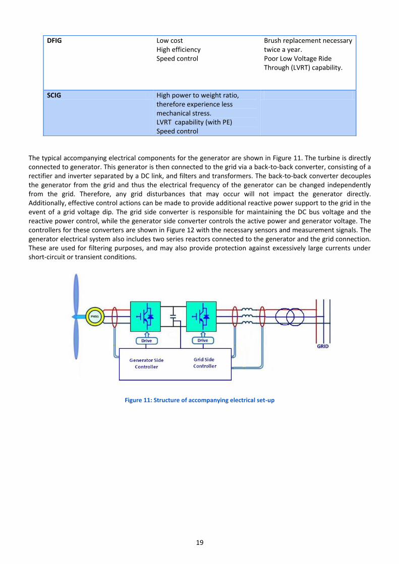
The typical accompanying electrical components for the generator are shown in Figure 11. The turbine is directly connected to generator. This generator is then connected to the grid via a back-to-back converter, consisting of a rectifier and inverter separated by a DC link, and filters and transformers. The back-to-back converter decouples the generator from the grid and thus the electrical frequency of the generator can be changed independently from the grid. Therefore, any grid disturbances that may occur will not impact the generator directly. Additionally, effective control actions can be made to provide additional reactive power support to the grid in the event of a grid voltage dip. The grid side converter is responsible for maintaining the DC bus voltage and the reactive power control, while the generator side converter controls the active power and generator voltage. The controllers for these converters are shown in Figure 12 with the necessary sensors and measurement signals. The generator electrical system also includes two series reactors connected to the generator and the grid connection. These are used for filtering purposes, and may also provide protection against excessively large currents under short-circuit or transient conditions.
Figure 11: Structure of accompanying electrical set-up
DFIG Low cost High efficiency Speed control
Brush replacement necessary twice a year. Poor Low Voltage Ride Through (LVRT) capability.
SCIG High power to weight ratio, therefore experience less mechanical stress. LVRT capability (with PE) Speed control

20
(a) (b)
Figure 12: Example of (a) generator side control (b) grid side control
The equivalent circuit model of a permanent magnet generator is shown in Figure 13. The generator voltage and currents have been transformed into d (direct) and q (quadrature) axis using the Park transformation.
Figure 13: Equivalent circuit of PM generator on the dq-rotating frame
The equation for the electromagnetic torque, Tem, in the permanent magnet generator is:
(30)

21
Flux linkage of the stator d-axis windings due to the flux from the rotor magnets
iq: q-axis current The terminal voltages of the generator in the d-q reference frame are given by (31) and (32)
(31)
(32)
Rs: Stator phase resistance id: d-axis current Ld: d-axis inductance Lq: q-axis inductance ωe(t): Electrical rotating speed (equal to the number of pole pairs multiplied by mechanical speed of the
generator)
3.2 TIDAL PTO
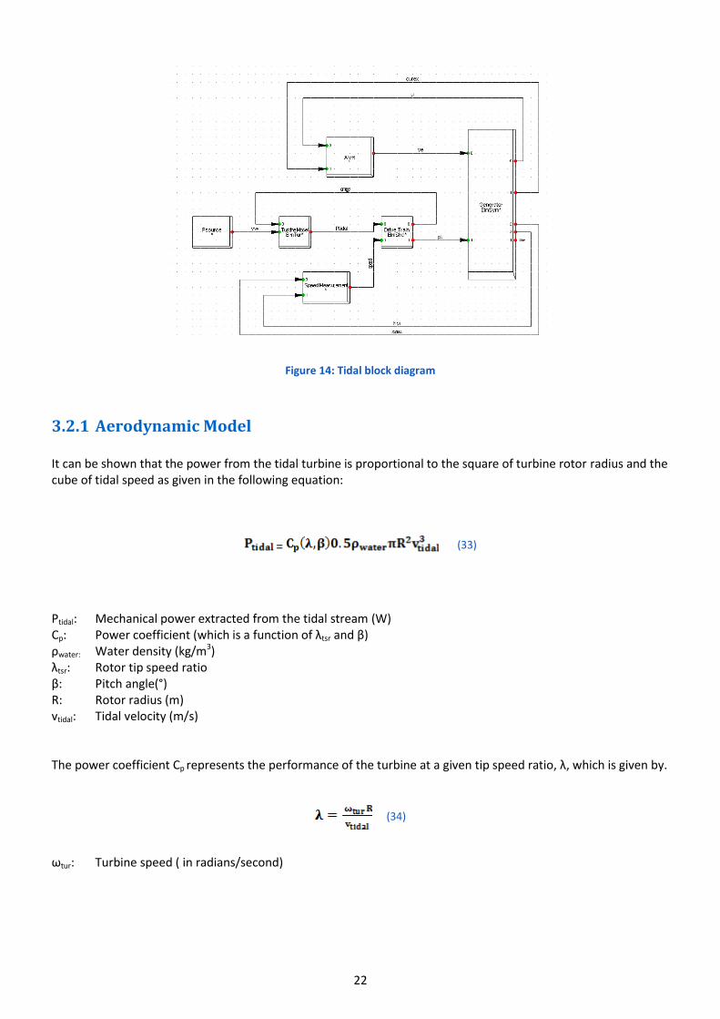
The operation of tidal turbines is synonymous to that of a wind turbine, but operating within a different fluid. Tidal energy has many benefits such as the fact that tidal currents are predictable, resulting in less grid integration issues. Seawater is over 800 times denser than air, therefore tidal power produces a greater energy density than wind for a given turbine rotor swept area. Several tidal PTO types exist such as Horizontal Axis Turbines, Vertical Axis Turbines, Oscillating Hydrofoils, Enclosed Tips (Ducted), Helical Screw, Tidal Kites, among others. Figure 14 illustrates the tidal turbine model as implemented in DIgSILENT PowerFactory. The model consists of the following component models; Psource model (input time series file of tidal current velocities), aerodynamic model, drive train model, generator with automatic voltage regulation (AVR), which maintains the terminal voltage of the generator, and a speed measurement sensor for the generator. The aerodynamic model and the derive train model are now described in more detail.
22
Figure 14: Tidal block diagram
3.2.1 Aerodynamic Model It can be shown that the power from the tidal turbine is proportional to the square of turbine rotor radius and the cube of tidal speed as given in the following equation:
(33)
Ptidal: Mechanical power extracted from the tidal stream (W) Cp: Power coefficient (which is a function of λtsr and β) ρwater: Water density (kg/m3) λtsr: Rotor tip speed ratio β: Pitch angle(°) R: Rotor radius (m) vtidal: Tidal velocity (m/s) The power coefficient Cp represents the performance of the turbine at a given tip speed ratio, λ, which is given by.
(34)
ωtur: Turbine speed ( in radians/second)

23
It can be seen from the sample Cp – λ tidal characteristic curve (Figure 15), there is an optimum operation point which occurs for a single value of tip-speed-ratio.
Figure 15: Sample tidal turbine Cp-lambda curve [13]
3.2.2 Drive Train Model The shaft model (Figure 16) [14] is a two mass model, with a large mass corresponding to the rotor inertia, Jrot, and a small mass corresponding to the generator inertia, Jgen. The shaft model, as implemented in DIgSILENT PowerFactory, is shown in Figure 17. The drive train converts the aerodynamic torque of the rotor onto the low speed shaft, Tshaft.
Figure 16: Tidal turbine drive train [14]
k: Stiffness coefficient c: Damping coefficient ηgear: Gearbox ratio

24
Figure 17: DIgSILENT PowerFactory Turbine shaft model
Similarly to wind turbines, the representative tidal turbine shown in Figure 18 contains three separate regions. Region I is below the cut-in speed, where the tidal current velocity is too low to turn the rotors and the turbine is unable to extract any power. In region II, the power extracted is proportional to the incident power on the rotor swept area. Region III is above the rated speed value, and the power extracted is controlled to be constant.
Figure 18: Tidal power curve

25
3.3 POWER SYSTEMS DYNAMIC MODELS As previously mentioned in Section 2.4, power systems simulation tools play an imperative role in ensuring that the grid integration of ocean energy devices does not negatively impact on the transmission grid stability and security, during both normal and faulted conditions. Furthermore, new grid code requirements are emerging, making the provision of dynamic power system simulation models mandatory for grid connection of renewable energy systems greater than 5MW. The provision of power system dynamic models allows the TSO to investigate how the installation of new renewable energy systems will interact with the grid, and what, if any, remedial design work needs to be carried out in order to maintain grid stability. There are numerous software packages available to investigate whether the ocean energy system satisfies grid code requirements; DIgSILENT PowerFactory, PSS/E, PSCAD, GE PSLF, SimPowerSystems, among others.
In the following section, DIgSILENT PowerFactory is used as an example case to demonstrate the methodology for creating a power systems dynamic model for an ocean energy device.
The power systems dynamic model consists of four main layers:
Overall PTO model:
The typical energy conversion processes of an ocean energy system are described in the Overall PTO model as shown in figure 18. This model is comprised of the wave source data input data, the Primary Power Capture model, and Prime Mover Unit. The wave source data consists of a time series of wave elevation height data or tidal speed. The Primary Power Capture process describes the means through which the ocean energy device interacts with the energy source, transferring energy from the waves or tidal currents to a medium which can be captured by the Prime Mover Unit, which converts the pneumatic power to the turbine’s mechanical power using the turbine’s performance characteristics. The Overall PTO model is then linked to the electrical network via the single line diagram.
Figure 18: PTO Overview depicted in DIgSILENT PowerFactory [15]
(PPC: Primary power capture, PMU: Pneumatic)

26
The single line diagram (shown in Figure 20), is a simplified way of representing a three phase power system. This layer shows an overview of the electrical components of the ocean energy system, which includes a generator, back to back to back converter (two PWM converters), dc capacitor, dc chopper, and two transformers. It also incorporates two series reactors connected to the generator and the grid connection bus. These are used for filtering purposes, and to provide protection against excessively large currents under short-circuit or transient conditions. Power system simulation tools typically contain libraries containing standardised schematics of these electrical components.
Figure 20: Ocean energy grid electrical system depicted in DIgSILENT PowerFactory
Electrical System Control This model contains the overall control of the electrical system (Figure 21). The measurement blocks are linked to specific components in the single line diagram in order to measure the generator speed, voltage, real and reactive power, grid voltage, and dc voltage. These measurements are then sent to PWM converter controllers, and are compared to the reference signals of power, reactive power or voltage, as appropriate, to determine the values of direct and quadrature currents to be sent to the PWM converters. In this simulation example, the generator side PWM converter is responsible for the DC bus voltage and the reactive power control, while the generator side converter controls the active power and generator voltage.
Figure 21: Control of electrical systems
27
Power Electronics Controllers Figure 22shows a more detailed look at the grid side PWM converter controller, which controls the grid reactive power and the DC bus voltage using proportional-integral (PI) controllers.
Figure 22: Example of grid side power electronics controllers
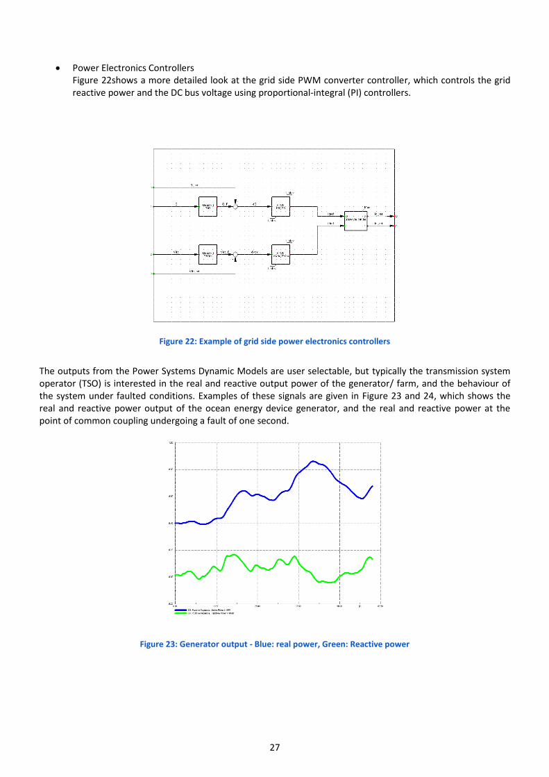
The outputs from the Power Systems Dynamic Models are user selectable, but typically the transmission system operator (TSO) is interested in the real and reactive output power of the generator/ farm, and the behaviour of the system under faulted conditions. Examples of these signals are given in Figure 23 and 24, which shows the real and reactive power output of the ocean energy device generator, and the real and reactive power at the point of common coupling undergoing a fault of one second.
Figure 23: Generator output - Blue: real power, Green: Reactive power

28
Figure 24: Blue: real power, Green: Reactive power at the point of common coupling during a fault
4 AGGREGATION MODELLING METHODS The approach to ocean farm aggregation may be undertaken in two distinct areas; ocean energy device interaction and aggregation of a farm for Power System studies. Ocean energy device interaction focuses on the system hydrodynamics and the interactions between the ocean energy devices. Any moving body in waves generates a diffracted/radiated wave which propagates in all directions around the body (Figure 25), known as the Park effect. Depending on the wave farm layout, areas of constructive and destructive wave interference will occur which will increase or decrease the power output from individual devices. Additionally, the spacing between devices can result in beneficial power smoothing in the farm power output quality if devices are spaced apart appropriately. This is due to individual waves reaching the devices at different times, introducing a time delay between the power outputs of the individual devices.
Figure 25: Device Interaction [16]

29
BEM-based numerical codes such as WAMIT, ANSYS Aqwa, Aquaplus are used to examine the hydrodynamic effects of device interaction. However, these studies are limited to arrays of 5 to 10 devices due to memory and CPU requirements. It is thought that for small arrays of less than ten devices of 10 to 20 meters typical dimension, and separating distance of 100 to 200 meters, the park effect may be neglected. For larger arrays of more than ten devices, the Park's effect becomes more prevalent, and the number of rows (devices perpendicular to the incident wave direction) in the ocean energy farm should be kept low, with as much distance between the devices as possible [16].
For aggregation models for Power System studies, the focus is different; these models focus on determining the
power output of an entire farm. The following section will focus on modelling an ocean energy farm from a PTO
and power systems perspective. The high level of accuracy usually demanded for hydrodynamic studies is not
required in power systems studies. Additionally, a detailed model of each individual device would be too
computationally intensive, and complex, therefore aggregating the ocean energy array into a smaller number of
models is desirable.
The wind industry can often serve as a useful source of knowledge for the wave energy. Wind farm are often
modelled by equivalent models, without significantly compromising the accuracy of the simulation results. In its
simplest from, a wind farm may be represented by a single equivalent model, where the wind turbines are
characterised by very small speed ranges from cut-in to rated power [17]. Therefore, the power of the aggregated
generator may be simply multiplied by the number of wind turbines. The small difference in wind speeds mean
that the mechanical components, gearboxes etc of the drive train may also be aggregated. This one equivalent
model is generally more suited to synchronous generators with stiff shaft systems. If irregular wind conditions
occur over the farm area, this will not be reflected in the model outputs.
In wind farms where the wind speed varies, the farm may be divided into several groups of turbines. The
groupings depend on the turbine characteristics, the wind profile and the distribution of the layout of the farm.
For each group of wind turbines the wind speed is considered uniform, and it is assumed that all the turbines are
exposed to the same turbulence level. It is not necessary that every group of wind turbines is composed of the
same number of wind turbines; it depends on the amount of turbines with the same characteristics. The drive
trains in each group may also be aggregated.
Similarly, for wave farms, the wave energy converters (WEC) will be grouped together in rows receiving the same
incident wave conditions (assuming the devices separating distances are large enough). Aggregating a wave farm
involves two separate steps:
Time shifting of the incident wave conditions so that the wave energy converters within the farm are modelled with the appropriate resource time series
Aggregation of the electrical equipment and the PTO systems, depending on directionality of the input wave conditions.
A method for time shifting the incident wave conditions is given in [18]. An array of six wave energy converters is shown in Figure 26, where one device is chosen as the reference device. A random time delay is applied to each of the other devices in order to represent the effect of device aggregation on the power output of the farm. Each time delay ΔTtotal consists of a constant time delay ΔT corresponding to a constant inter-WEC distance D, to which a variable time delay ΔTiis subtracted. This latter time delay is intended to introduce a certain degree of randomness in the spatial scattering of the devices with the farm, and correspond to a variable distance ΔDi.

30
Figure 26: Schematic illustration of the spatial scattering of wave energy converters (WEC)
Time delays are calculated based on typical value of the average wave group speed vg, estimated from the energy period Te of a given sea-state [19]:
(35)
Te is used instead of other common parameters; the peak period, Tp, or the zero-crossing period, Tz, as it represents the energy propagation speed between two WECs more accurately. This approach provides a reasonable estimation for the typical speed of any wave group during a given sea-state. The time delay ΔTtotal was calculated as:
(36)
ΔTtotal: Time delay ΔT: Constant time delay
ΔTi: Variable time delay
and (37)
D: Distance between wave energy converters (m) νg: Wave group speed

31
Different wave directions can be simulated by the assignment of time delays. In Figure 27, for simulating the wave direction of Case B, all generators belonging to the same feeder would have the same time delay, and therefore these WECs may be aggregated together. Whereas for Case A, all generators belonging to the same feeder will have a different time delay, and may need to be modelled separately. The aggregation effect between different device clusters or farms (spaced by few kilometres) can also be modelled using the same method and applying an additional time delay Δtcluster.
Figure 19: Wave farm electrical drawing [18]
As mentioned earlier, the distribution network in the ocean energy farm should also be should be aggregated,
ensuring that the resulting impedance of the aggregated cables should be equivalent to the original impedance.
As an example, Case B will be used as an example of aggregating the electrical system. Firstly, the equivalent
resistance, Requiv, reactance, Xequiv, and susceptance, Bequiv, of each feeder should be found using the following
equations. The subsea shore cables may be left as is.
(38)
(39)
(40)
mupstream: Index (number of turbines upstream)
n: Number of turbines in a string

32
Aggregation of the electrical equipment should also be carried out: o Generators: The number of parallel generators in each row should be changed, which increases the active
power of the model. In the given example, this is n = 5.
o Transformers: Increase the power rating by "n" times.
o Series Reactors: Increase the power rating by "n" times and carry out one of the following options:
o Multiply the copper losses by "n", or
o The values of resistance and reactance should be divided by "n".
o PWM Converters, grid measurement devices, reactive power compensation ratings:Increase the power
rating by "n" times
An example of the effect of aggregating a wave farm on the accuracy of the load flow results for the power
system is shown in Table 3. In this example, a wave farm is aggregated from 20 generators to 4 generators
(Figure 28). Evidently, the accuracy of the generator real power and the injected current are not affected by the
aggregation procedure. However, there is a slight difference in the values of the reactive power, which may be
due to slight inaccuracies in summing the susceptance of the feeder cables.
Table 3: Effects of aggregation on Power System studies accuracy
Physical Parameter Full Ocean Energy FarmFactor Aggregated Farm
Number of Generators 20 4
Generator Power 39.99MW 39.99MW
Reactive Power (MVar) 18.97 MVar 18.92 MVar
Injected Current (kA) 0.38kA 0.38kA
Figure 28: Single line diagram aggregating wave farm into equivalent model (DIgSILENT PowerFactory)

33
Aggregation of the PTO equipment is also necessary. In most power systems simulation models, many of the
signals are in per unit format; the parameters in the component do not need to be changed as they operate in per
unit with respect to the new scaled-up power rating reference. Therefore minimal steps are used to aggregate the
PTO system. For example, generator control laws, such as power – speed reference control laws, should be
upscaled.
5 VALIDATING PTO MODELS WITH EXPERIMENTAL TESTS
5.1 INTRODUCTION
Experimental tank testing of scaled prototype ocean energy converters is a key phase in the progression of ocean energy research. It allows the performance and characteristics of designs to be investigated in a controlled environment, and verifies that the designs operate as theoretically predicted. Many other characteristics may be investigated using tank testing, such as the pitch, heave and surge motion, loading on the device, and survivability.
Validating PTO models with experimental tests is an important task to confirm the validity of the scaled tests, so future testing and progression to full scale models can be performed with greater confidence. Given the limited availability of large and deepwater basins, experimental tests are typically carried out at scales from 1/50 to 1/10. The appropriate selection of the model scale is considered under both economic and technical constraints, which must take into account the size and depth of the wave tank, and the wave generating capabilities. These experimental results must be adjusted in order to demonstrate the performance of the full scale device. Additionally, scaling of the devices results in some inaccuracies when modelling various components of the PTO system. These aspects will be examined in the following sections.
5.2 DATA SCALING This section describes the theory and concepts of scaling when applied to electrical test rigs. Scaling concepts must be understood in order to correctly translate the input data to the scale of the test rig and to translate the output data back to the full scale of the prototype being examined.
5.2.1 Input test data is often from scaled tests Despite advances in numerical device hydrodynamic models and wider available of increased computational power, the building of physical scaled models persists. These models are tested both in wave basins and at sea. Even at sea, scaled models are typically built before moving to full-scale prototypes. The high risk and high costs associated with full scale sea trials do not allow for iterative at sea-design. All these physical tests of scaled models produce data sets which are then used in the electrical test rig environment.
5.2.2 Test rigs are typically not at full scale There is a growing appreciation of the impact of coupling between the mechanical and electrical systems in ocean energy devices. As a result more electrical test rigs are being built specifically to test these devices by both academic centres and industrial companies. These rigs are often connected at distribution level voltages and are

34
built at scaled power levels. Even the more costly megawatt test rigs may not exactly mirror the inertia, stiffness or other subtleties of a full scale prototype. In summary, scaled input data from wave basins or from scaled sea-trials need to be suitably adjusted to the scale of electrical test rigs. The results gathered from the electrical testing then need be adjusted a second time to yield the results expected from a full scale prototype. Before describing the correct steps to scale the data, some background theory is presented on (i) similitude and (ii) dimensionless numbers.
5.2.3 Principle of Similitude Similitude describes how well a model represents real-life conditions. Similitude is considered under three headings;geometric, kinetic and dynamic similitude, i.e. shape, force and movement. Geometric similitude is achieved if a fixed ration relates every length of the model to the corresponding length of the full-scale prototype. Kinetic similitude requires that the fluids or air moving around and through the model move in the same way they move around and through the full scale prototype. Finally, dynamic similitude is the similitude of forces. The forces applied to and the model must be scaled versions of those applied to the full-scale model. A model is said to have perfect similitude if it meets the three requirements of geometric, kinetic and dynamic similitude. It is not always possible to achieve this with models; certain forces are not easily scaled. For example, scaling gravity is tricky and requires significant effort and expensive test equipment, e.g. centrifugal in Grenoble.
5.2.4 Dimensionless numbers Several fields of engineering rely heavily on dimensionless numbers, none more so than fluid dynamics. Since physical laws are homogenous ( i.e. they do not depend on the choice of basic units) the law is valid in any system of dimensions. When considering scaled models this principle is vital. In scaled tests, dimensionless numbers ensure the force ratios are similar. If the dimensionless number calculation, as in equation 41, of both the model and the prototype are equal the force ratio is equal.
(41) For perfect similitude all forces ratios have to be equal. In any model there are many forces at work including
inertial forces,
gravitational forces,
viscous forces,
elastic forces,
pressure forces, and many more.
Achieving similitude simultaneous of all these forces is extremely difficult without the scale being very close to unity. Therefore model builders need to determine the important dominant forces and attempt to keep those scaled in the correct ratio. Several force ratios have proven to be of interest and of specific use in different engineering problems, so much so that they have been given the names of the men who instigated their use.

35
Table 4:
Ratio of Inertia …
Definition of Dimensionless number
Name of Dimensionless number
Named after
… and Gravity
Froude Number William Froude
(1810-1879)
… and Viscosity
Reynolds Number Osbourn Reynolds
(1842–1912)
… and Elasticity
Mach Number Ernst Mach (1838-1916)
… and Drag
Keulegan–Carpenter Number
Garbis H. Keulegan and Lloyd H. Carpenter
… and Surface Tension
Weber Number Moritz Weber (1871–1951)
Surface waves in the ocean are gravity driven. The strong dependency on gravity, g, can be seen in the equations in Table 5 describing the surface motion of a sea. Therefore, in many ocean energy device models the ratio of inertial force to gravitational force is the most important force ratio of interest. Therefore, models of devices that engage with ocean waves are built according to Froude scaling rules.
Table 5:
Shallow Water Intermediate Water Deep Water
Wave
Property
Wave Length λ
Dispersion
Relation
Celerity c
Table 6 shows the scaling factors for a selection of physical parameters required to have a valid Froude scaled model. These relationships easily derived from when the Froude number of the model and the Froude number of the prototype are kept constant. Similar tables of parameters can be calculated for different scaling methods e.g. Reynolds or Mach.

36
Table 6: Froude Scaling Rules for a selection of physical parameters
Physical Parameter Multiplication Factor
Length λ
Time
Structural Mass λ3
Inertia λ5
Force λ3
Torque λ4
Linear Velocity
Angular Velocity
Linear Acceleration 1
Angular Acceleration
Pressure λ
Power λ 3.5
5.2.5 Scaling for electrical testing for ocean energy devices In the previous section the theory behind scaled testing has been presented. The following section will describe how this theory is applied to electrical testing of ocean energy devices. As described in 5.2.1 and 5.2.2 above, the source data for the laboratory test is often not full scale data and the test equipment is also not a full scale. Therefore, there are often three scales to be considered when carrying out electrical testing; source data scale, full scale and electrical test rig scale. These are represented graphically in Figure 29.
Figure 29: Three scale zones typically involved in electrical testing of ocean energy devices

37
The scale of the source data, ,is known and fixed, however there is a degree of freedom in selecting a suitable test rig scale , . The same device model could be tested at different scales on the electrical test rig,
e.g. 1/20th scale for normal operation but 1/40th for high power wave conditions. The user must select a suitable test rig scale value to suit the test rig being used. As well as scaling the power, other parameters need to be considered. The following sections outline an approach to fitting scaled test data to electrical test rigs.
5.2.5.1 Select the type of scaling
As discussed in section 5.2.4, the method of scaling must be carefully selected to correctly represent the dominant forces of the device under test.
5.2.5.2 Scale according to Power ranges
The power range of the full scale device and that of test rig will largely determine the test rig scale, .The peak
mechanical power at the test rig must be within the power range of test equipment. This is usually the first step at determining a suitable scale for the experiment.
5.2.5.3 Check other parameters are within range
Once a first guess at a suitable scale has been determined, other parameters need to be checked to ensure they are within the physical limits of the test rig. All electrical test rigs have limited speed, torque, inertia and power ranges (Figure 30). The inertia of the test rig may be fixed or adjustable to discrete levels of inertia using a gear-box and flywheel combination. Given these physical limitations, certain devices may not fit every electrical test rig. If the experiment values for speed, torque, power and inertia are within range testing can begin. Otherwise some simple options may prove useful.
Figure 30: Important parameters to consider for electrical testing
5.2.5.4 Optional steps to increase ranges of test rig
Two options are presented below to help ‘fit’ the experiment to the electrical test rig being used. o Virtual Gear Box o Virtual Inertia

38
Virtual Gear Box If the speed and torque parameters do not fit, then a virtual gear box can be added. The scaled model running on the system controller e.g. Programmable Logic Controller (PLC) can operate at a different speed and torque to that of the electrical test rig. Note the gear-ratio squared relationship for inertia shown in Figure 31.
Figure 31: Scaling – with virtual gear box
Virtual Inertia This method expands the range of model inertia values that can be tested on a given electrical test rig. An additional inertia is added the virtual device model that is controlling the motor.
5.2.6 Summary guide to scaling for electrical test rigs 1. Determine dominant forces 2. Select scaling rule (e.g. Froude) 3. Determine power range of Full scale 4. First guess at test rig scale based on power scaling 5. Examine other parameters based on this scale. (e.g. speed, torque, inertia) 6. If all parameters are within range begin testing 7. Otherwise, the following options may help ‘fit’ the full scale data to the test rig limitations
7.1. Adjust the first guess test rig scale 7.2. Add a virtual gear box 7.3. Add virtual inertia to the model

39
5.3 LIMITATIONS IN VALIDATING PTO MODELS WITH EXPERIMENTAL TESTING While the previous section dealt with validating electrical PTO systems, this section examines some factors to consider when validating other PTO systems. There are a number of challenges that exist when attempting to validate numerical PTO models with experimental tank testing, and therefore should be bore in mind when examining results. There are a number of challenges that exist, including:
Successfully replicating the PTO systems in small scale devices, therefore leading to discrepancies when comparing to the PTO numerical models
Correctly analysing the measurements results
Understanding the inaccuracies from measurement sensing equipment The scale factor for a model is usually chosen as an optimisation between cost and technical accuracy. Most available test tanks cannot produce the period or wave height required; therefore tests are performed at scales that are less than ideal, resulting in scaling effects in the PTO systems. Scale effects occur due to non-identical force ratios which arise between a scaled model and its full scale model and result in deviations in behaviour [20]. Generally, the larger the scale ratio of the model, λ, the more the incorrect modelled force ratios deviate from the full scale ratios and larger scale effects occur. Additionally, the compressibility of the air water mixture can be different in model and full scale device and therefore causing potential scale effects. Generally, the PTO system is not scaled in small scale devices, but instead damping is introduced, such as orifice plates or pneumatic cylinders, which is easier to quantify. In cases where the PTO system is scaled, the scaling effects may result in misleading measured quantities. For example:
Turbines exhibit lower efficiencies due to fixed friction losses at smaller scale [10]
Hydraulic cylinders are not easily replicated at small scale, and show increased sticking friction
In overtopping devices, the surface tension and the compressibility in the buoyancy compartment are not scaled correctly with Froude scaling [10]
Research Centre Ocean
The reliability and quality of the measurement data should be taken into consideration, and insurances made that the sensors are suitably calibrated. Analysis of the measurements test results should also be carried out with care. Standard mathematical approaches may be used to investigate data, and some recommendations for analysing these results are given in [21].

40
6 REFERENCES [1] MRTN-CT-2004-50166 , Wavetrain Research Training Network Towards Competitive Ocean Wave Energy RTN Deliverable 21: System Identification: Pilot Plant Simulation Models [2] D. O’ Sullivan, D. Mollaghan, A. Blavette and R. Alcorn (2010). “Dynamic characteristics of wave
and tidal energy converters & a recommended structure for development of a generic model for grid connection”, a report prepared by HMRC-UCC for the OES-IA Annex III. [Online], Available: www.iea-oceans.org.
[3] J. Cruz, ed. Ocean Wave Energy: Current Status and Future Perspectives; Springer,2008. [4] A.P. McCabe, A time-varying parameter model of a body oscillating in pitch, Applied Ocean
Research, Volume 28, Issue 6, December 2006, Pages 359-370 [5] Josset, C., A. Babarit, and A. H. Clément. "A wave-to-wire model of the SEAREV wave energy
converter." Proceedings of the Institution of Mechanical Engineers, Part M: Journal of Engineering for the Maritime Environment 221.2 (2007): 81-93.
[6] A. F. de O. Falcão, "Wave energy utilization: A review of the technologies", Renewable and
Sustainable Energy Reviews, Volume 14, Issue 3, April 2010, page 899 [7] Curran, R., T. J. T. Whittaker, and T. P. Stewart. "Aerodynamic conversion of ocean power from
wave to wire." Energy conversion and management 39.16 (1998): 1919-1929. [8] A. F. de O. Falcão, and R. J. A. Rodrigues. "Stochastic modelling of OWC wave power plant performance." Applied Ocean Research 24.2 (2002): 59-71. [9] D.P. Cashman, et al. "Modelling and analysis of an offshore oscillating water column wave energy
converter." Proceedings of 8th European Wave and Tidal Energy Conference. 2009. [10] Tedd, James, and Jens Peter Kofoed. "Measurements of overtopping flow time series on the
Wave Dragon, wave energy converter." Renewable Energy 34.3 (2009): 711-717.
[11] Meinert, P; User manual for SSG power simulation 2; Hydraulics and Coastal Engineering, 1603-
9874, 44 (June 2006) Department of Civil Engineering, Aalborg University [12] D. O'Sullivan, A. W. Lewis. "Generator Selection and Comparative Performance in Offshore
Oscillating Water Column Ocean Wave Energy Converters." Energy Conversion, IEEE Transactions on 26.2 (2011): 603-614.
[13] Chul-Hee Jo, Jun-Ho Lee, Yu-Ho Rho, Kang-Hee Lee, "Performance analysis of a HAT tidal current
turbine and wake flow characteristics", Renewable Energy, Available online 26 September 2013

41
[14] A. D. Hansen et al,” Dynamic modelling of wind farm grid interaction”, Wind Engineering, Vol. 26, no. 4, 2002
[15] D. Mollaghan, S. Armstrong, D. O’Sullivan, A. Blavette, R. Alcorn. "SEAGRID: A New Dynamic
Modelling Tool for Power System Analysis of Ocean Energy Devices", 4th International Conference on Ocean Energy 2012, 17th -19th October 2012.
[16] A. Babarit, “On the park effect in arrays of oscillating wave energy converters”, Renewable
Energy, Volume 58, October 2013, Pages 68-78. [17] J. Conroy, R. Watson. "Aggregate modelling of wind farms containing full-converter wind turbine
generators with permanent magnet synchronous machines: transient stability studies." Renewable Power Generation, IET 3, no. 1 (2009): 39-52.
[18] A. Blavette, M. Egan, D. O'Sullivan, T. Lewis, Dimensioning the equipment of a wave farm: energy storage and cables. In Proceedings of the EVER13 Conference, Monaco, 2013.
[19] J. Falnes, “Ocean Waves and Oscillating Systems: Linear Interactions Including Wave-Energy
Extraction”, Cambridge University Press, 2002.
[20] V. Heller, "Scale effects in physical hydraulic engineering models", Journal of Hydraulic Research, Vol. 49, Issue 3, 2011 [21] B. Holmes, “Tank Testing of Wave Energy Conversion Systems”, EMEC, 2009