REPORT OF THE 2009 ICCAT WORKING GROUP ON ... Collect. Vol. Sci. Pap. ICCAT, 65(5): 1851-1908 (2010) 1851 REPORT OF THE 2009 ICCAT WORKING GROUP ON STOCK ASSESSMENT METHODS (Madrid,

SCRS/2009/010 Collect. Vol. Sci. Pap. ICCAT, 65(5): 1851-1908 (2010)

1851

REPORT OF THE 2009 ICCAT WORKING GROUP ON STOCK ASSESSMENT METHODS

(Madrid, Spain - March 11-14, 2009)

SUMMARY

The Meeting was held in Madrid, Spain from March 11 to 14, 2009. The objectives of the meeting were to evaluate the merits of alternative CPUE standardization methods and make progress towards the completion of a CPUE Standardization Manual, to investigate the influence of life history characteristics, environmental variability and gear selectivity on Status Determination with respect to the Convention objectives and to address other methodological matters related to stock assessment quality control procedures.

RÉSUMÉ

La réunion a eu lieu à Madrid (Espagne) du 11 au 14 mars 2009. La réunion avait pour objectif d’évaluer les avantages de méthodes de standardisation alternatives de la CPUE, de réaliser des progrès en ce qui concerne la réalisation d’un Manuel de standardisation de la CPUE, de chercher à déterminer l’influence des caractéristiques du cycle vital, de la variabilité environnementale et de la sélectivité des engins sur la détermination de l’état par rapport aux objectifs de la Convention, et d’aborder d’autres questions méthodologiques relatives aux procédures de contrôle de la qualité des évaluations de stocks.

RESUMEN

La reunión se celebró en Madrid, España, del 11 al 14 de marzo de 2009. Sus objetivos eran evaluar los beneficios de métodos alternativos de estandarización de la CPUE y avanzar en la finalización del Manual de estandarización de la CPUE, investigar la influencia de las características del ciclo vital, la variabilidad medioambiental y la selectividad del arte en la determinación del estado de los stocks con respecto a los objetivos del Convenio y abordar otras cuestiones metodológicas relacionadas con los procedimientos de control de calidad de las evaluaciones de stock.

1. Opening, adoption of Agenda and meeting arrangements Mr. Driss Meski, ICCAT Executive Secretary, opened the meeting and welcomed participants. The meeting was chaired by Dr. Victor Restrepo. Dr. Restrepo welcomed the Working Group participants, reviewed the objectives of the meeting and proceeded to review the Agenda which was adopted with minor changes (Appendix 1). The List of Participants is attached as Appendix 2. The List of Documents presented at the meeting is attached as Appendix 3. The following participants served as Rapporteurs for various sections of the report:

Section Rapporteurs

1, 5, 7 P. Pallarés 2 V. Ortiz de Zárate and C. Minte-Vera 3 J. Neilson, M. Schirripa and E. Rodríquez-Marín 4 S. Cass-Calay, A. Di Natale and G. Scott 6 G. Scott

1852

2. Manual for CPUE standardization The Working Group Chair reminded the meeting participants that the outline of the ICCAT CPUE standardization manual has been available for some time (see Appendix 4 of Anon. 2008). However, the contents of the manual have not been drafted yet. In the ICCAT Manual available at the website, there is an introductory chapter on CPUE standardization to be used for ICCAT stock assessment. During the meeting, several documents about CPUE standardization which were prepared for a workshop in the United States (SouthEast Data, Assessment, and Review process, SEDAR, http://www.sefsc.noaa.gov/sedar/) were presented as information documents. The Group found that the content of these documents (attached as Appendix 4) was very interesting and that the same material could potentially be used for the ICCAT manual on CPUE standardization. These scientists and others who are interested in collaborating on this effort were encouraged to work towards the completion of a first draft of the manual in time for the 2009 SCRS meeting. 3. Review of methods to address species targeting and gear/species overlap during CPUE standardization The Group received three working papers that related to targeting in CPUE analyses. It should also be noted that recent reports of the Stock Assessment Working Group contain useful additional material relevant to this topic (Anon. 2001; Anon. 2004). Simulation Testing In SCRS/2009/028, the authors explored the effects of targeting, where fishing effort is directed towards one species as opposed to another, which can introduce bias into CPUE time series. In recognition of this fact, the ICCAT working group on assessment methods has recommended testing alternative standardization methods. Simulation techniques were shown to offer an objective and scientifically sound means to explore this problem. Data from simulations can subsequently be analyzed with any number of standardization methods to quantify the performance of each alternative. The authors presented a simple, two species-one gear approach that demonstrated a simple study design using simulated data. They then considered an arbitrary longline fleet catching yellowfin tuna and blue marlin whose distributions were assumed proportional to the annual average spatial distributions of catch per unit effort by month in the ICCAT longline data. The spatial distributions of otherwise arbitrary longline sets were input by year, month, latitude and longitude. Half of the simulations assumed no targeting, and the simulated effort was equally divided between areas of high yellowfin tuna and blue marlin catch rates. The other half of the simulations began with equal effort between the two species but targeted yellowfin tuna in the last half of the time series. The simulated population trajectories of the two species were either assumed to have no trend or to follow the trends estimated from the last assessments. Even with these relatively simple simulations, it was obvious that targeting substantially biased the CPUE time series. Such simulated data sets provide the opportunity to test alternative standardization methodologies to remove the biases introduced by species targeting. The simulation model employed, described as LLSIM at the end of this section, (a successor to the SEEPA program that is part of the ICCAT software library: http://www.iccat.int/en/AssessCatalog.htm) also provides for the evaluation of much more complicated problems. However, the authors proposed that studies progress from simple to more complex assumptions to minimize possible misinterpretation of results. The paper SCRS/2009/028 pointed out some cases when the CPUE standardization was not able to recover the true simulated trend, even given perfect information on when the shifting in target was occurring during the time series. One possible explanation is that the software used to standardize the CPUEs might treat unbalanced designs in a different fashion. The Working Group decided that further exploration on the effect of software on the standardization of CPUE should be performed during this meeting. For this exploration, the simulated data used was that on blue marlin (hereafter BUM) generated when population trajectories were assumed to follow the trend estimated in the last stock assessment and the shift into targeting yellowfin tuna occurred in 1975. The delta-lognormal approach was computed in SAS (Shono, 2001) and compared to the original R results. Both standardizations were biased and produced higher relative CPUE then the true relative biomass before 1975 and lower after 1975. Although there could be some differences between the source code used in the two analyses, the Group concluded that the choice of statistical software was probably not responsible for the problem of biased representation of the trend in CPUE. Another possible explanation for the bias was that the rareness of the blue marlin species was resulting in an empirical distribution of catch per set that could not be represented by a lognormal distribution even after the zeros are excluded (see Figure 4 lower panel in SCRS/2009/028). A more appropriate distribution to describe

1853

these data may be the Poisson distribution. Therefore the BUM data set was standardized using GLM procedure in R with the Poisson family. Two models were fit, with and without target as a factor explanatory variable. Similarly to the original models, both Poisson models had month and year as factors and latitude and longitude as continuous variables. The year effect estimates for both models differ only slightly between them and had the similar bias in trend that emerged when the delta-lognormal approach was used (Figure 1). The data might be more aggregated than expected by a Poisson distribution, and may be better described by other distributions. For future investigation of this issue, these data are available through the Secretariat. Also, a new data set should be produced with higher expected catches for blue marlin to explore whether the rareness of the species is the causing the bias. Dynamic Factor Analysis (DFA) In SCRS/2009/030, the author explored the usefulness of Dynamic Factor Analysis (DFA) to detect common patterns in the sets of CPUEs for Atlantic yellowfin (Thunnus albacores) and for eastern Atlantic skipjack (Katsuwonus pelamis), respectively. For yellowfin, the most appropriate model, in terms of AIC, identified two common trends. The 10 yellowfin CPUE series could be divided into three groups based on factor loadings. The grouping corresponds in part to the geographic location of the fisheries (i.e., the western Atlantic area for group 1 and the northeast tropical Atlantic region for group 2). The fact that the first group is constituted by CPUEs obtained from three different fishing gears (pole and line, purse seine and longline), operating at different depth levels, suggests that the regional trend reflects more a sub-population response to a local exploitation rate than to environmental conditions. In light of the present results, the CPUEs should be combined respectively into two regional indices before performing a unique combined index. For skipjack, results are less conclusive and further studies with explanatory factors are required to account for the fact that this species is seldom targeted by the tuna fisheries. The Group discussed the advantages and drawbacks of introducing increasing complexity into catch rate analyses. On the one hand, it was noted that more information and CPUE series is not always helpful, particularly when divergent and unexplained patterns are noted. On the other hand, it was pointed out that for spatially complex stocks, having discrete indicators of subpopulation exploitation rate can be very helpful, if sufficient data exist. The Group also commented that the reason that the skipjack results were less conclusive may be related to the impacts of FADs on catchability for this fishery. It was also noted that the various CPUE series could be targeting fish of different size. An empirical approach SCRS/2009/031 contained an examination of alternative methods to describe targeting in the Canadian pelagic longline fishery. Over the past decade, that fishery has evolved from a traditional swordfish fishery concentrated along the continental shelf edge to a more mixed fishery that targets swordfish and “other” tunas (albacore, bigeye and yellowfin). The spatial distribution of the fishery now also includes a higher proportion of trips made further offshore, in relatively warm Gulf Stream waters. A fishing trip is considered to be directed for swordfish if the total landed weight of swordfish exceeds that of tuna. Recent developments in the Canadian catch-effort database allow an examination of catch rates at the set level, thereby offering the potential for consideration of different target variables, such as bait type or sea surface temperature. The authors concluded that all three potential targeting variables (proportion of swordfish catch weight, SST, and bait) gave plausible and generally comparable results for swordfish-targeted trips. However, the alternate target variables did not explain more of the observed variation in catch rates than the model which incorporated the traditional method used for targeting. Additionally, while it is evident that set-specific differences can exist within fishing trips, the number of trips including multiple bait types is relatively small. Set level detail is available only for the portion of the catch rate series since 1994, and in order to utilize set details in the standardization the early part of the time series (1988-1993) would have to be omitted. The authors therefore recommended that the current practice of using the traditional method of swordfish targeting be retained in the Canadian CPUE for the upcoming stock assessment. The Group noted that including both bait and surface temperature together could be a useful approach, and could be investigated further.

1854

Longline fishery simulator (LLSIM) In addition to the three working papers described above, the Group received a presentation on a longline fishery simulator (LLSIM). The presentation noted that at the Assessment Methods Working Group Meeting in Shimizu, Japan in 2003 (Anon. 2004), the Working Group gave priority to use simulation to develop data sets for testing habitat standardization (HBS) versus GLM for standardizing CPUE for billfish caught on longlines. Initially the simulations were to use the same assumptions that were actually being used in the HBS for the Japanese longline data at the time. To accomplish this task, a longline data simulator (LLSIM) was developed. The first sets of simulated data from LLSIM were provided to the ICCAT Billfish species working group in preparation for its 2005 Data Preparatory Meeting in Natal, Brazil (Goodyear 2006a). The working group applied the available standardization methods to attempt to recover the “true” population trends from the simulated longline catch and effort data. None of the methods applied recovered the underlying true population trend. Subsequently, extensive analyses of the LLSIM code were performed as well as the inputs arising from the specifications adopted at the Shimizu meeting of the Methods Working Group. The results were presented at the September-October 2005 Madrid meeting of the ICCAT SCRS (Goodyear 2006b). The results implicated features of the Japanese data used in the simulations as major impediments to CPUE standardization in the simulated datasets. Currently, the code is dimensioned for six species with up to four behaviorally different sex/age groups each, and up to 50 gear types. The spatial dimensions reflect the Atlantic Ocean at a scale of 1 degree latitude and longitude with 64 depth layers from the surface to 640 m depth. The model is flexible in that it can be used to test a number of different problems related to longline CPUE standardizations. It is anticipated that it will be applied to develop data sets to test the statistical habitat standardization method (StatHBS) and various alternatives for including species composition of the catch as a method to account for targeting effects in the standardization of CPUE. The Group noted that as shown in SCRS/2009/028, LLSIM offers important capabilities for the investigations of catch rate standardizations, including targeting and gear/species overlap. To identify potential follow-up work from this meeting, the Group reviewed recent species stock assessments to identify priority problems involving catch rates and the impacts of targeting. Future works It was decided that the clustering methodology (Hazin et al. 2007a and Hazin et al. 2007b) used in the most recent swordfish assessment (Anon. 2007) would perhaps be a useful candidate. The group recognized a recommendation made during the review of that assessment:

Discussion of this approach resulted in a recommendation to investigate the method through simulation to permit evaluating the potential sources of bias in approach. Such simulations have been carried out for simpler methods which use catch of other species to index the degree of targeting (Anon. 2001). That set of simulations found that certain approaches using catch of other species could lead to serious bias in measures of relative abundance. The Group was concerned that the methods may have introduced a positive bias in the inferred relative abundance trend and believes that the pattern resulting may be an overly optimistic representation of the recent trend in southern Atlantic swordfish biomass.

Based on this recommendation the group set out to design a simulation study to test the veracity of the clustering methodology by evaluating (1) any potential biases inherent in this method, and (2) if any biases did exist how they would carry forward when including the clustering factor in the GLM standardization of the CPUE time series. The Group determined that a simulation employing six frequently encountered ICCAT species would be appropriate. Targeting would be simulated by assuming that fishers had accurate knowledge of the species geographic distribution and would change their target species by changing locations and directing more effort in those areas with known higher abundances. In an effort to begin with a simple design and to keep the results tenable, one gear configuration consistent over time would be used. The simulation results would be output such that the target species of each set would be known with certainty. While this feature needs yet to be implemented in the model, the author (Dr. Goodyear) assured the group that this could be done in a short time. Four simulations will be run, similar to those presented in SCRS/2009/028: (1) no trends in the simulated populations, (2) no targeting, (3) inconsistent trends in the population, (4) include targeting. The Group went on to discuss the various aspects of how targeting should be scheduled with regard to annual and/or monthly variation. This has yet to be worked out. The Group also agreed that the study should be conducted “blindly”, which is to say that the analysts should not be provided the true targeting information during their analysis. Furthermore, the data

1855

sets should have reasonable degree of similarity to the actual practices of the fleet being simulated, but not so close as to make the nature of the targeting an already known quantity. Species will likely be referred to with generic names so as not to bias any results. 4. Influence of life history characteristics, environmental variability and gear selectivity on Status

Determination with respect to the Convention objectives Document SCRS/2009/29 described a framework for examining the influence of life history characteristics and other sources of variability on stock status determinations with respect to ICCAT Convention (or other) objectives. The authors point out excursions below the expected BMSY can occur even in a fishery not undergoing overfishing (e.g. due to fluctuations in recruitment and other biological/environmental conditions). Therefore, it may be logical to define a “target” as a level that will accommodate natural variations of stock biomass without jeopardizing the health of the stock or the Convention objectives. If so, it may also be also useful to define a “limit” reference point less than the “target” benchmark, to use as a trigger for (accelerated) management actions. Under the current ICCAT convention fish stocks are managed with the objective of “maintaining the populations of these fishes at levels which will permit the maximum sustainable catch (MSY) for food and other purposes”. This language could be interpreted that FMSY is a “target” objective for each stock unit. Alternatively, more modern (than the ICCAT Convention) international instruments can be interpreted to mean MSY benchmarks should be treated as limit reference levels which should not be exceeded. This simulation framework demonstrated in SCRS/2009/029 allowed evaluation of possible biomass limits (Blim) in reference to whether the limit will likely trigger a (“false positive”) response (indicating that the stock is overfished when it is simply undergoing “normal” variability in recruitment) or whether the limit will fail to trigger a response (“false negative”) when the stock is being overfished and the limit is set too far away from the target to positively identify overfishing status. In the example given in the paper (loosely based on northern albacore) a notable result was the long recovery period required to rebuild SSB to a target level, even at relatively low levels of SSB depletion, making discrimination of overfishing effects from natural variation difficult unless the degree of overfishing (and subsequent depletion) is large. The Working Group discussed the difficulty in evaluation of the appropriate limits and targets without some policy guidance on the tolerable level of risk of either a false positive or false negative response. While it is possible to select a biomass limit below BMSY which offers low odds of ‘false positives’, this could be but at the expense of non-negligible odds of ‘false negatives’. While SCRS/2009/029 did not conduct a statistical ‘power analysis’, the simulation framework used makes it possible to do such work and the Working Group recommended this be pursued through simulation to provide additional information for use in policy setting. One advantage of setting a target biomass above BMSY is that such targets can be established at levels which simultaneously result in low odds of biomass excursions below BMSY and low odds of ‘false negatives’. One result of the analysis provided in SCRS/2009/029 was the variability in SSB relative to the expected level of SSBMSY was insensitive to the proxy F level used for MSY calculations and the selectivity pattern modeled. This result is similar to the finding in SCRS/1998/120. In view of this, the WG decided to examine the expected variability in SSBMSY in ICCAT stocks for which recent age-based assessments were available (see Appendix 5). In the cases of stocks for which age-structured assessments are not the primary basis for management advice (e.g. N SWO, BET, BUM, WHM, etc.), it was recommended that the use of simulation methods following those described in Goodyear (1999) be applied to compare with the computations made by the Working Group at the meeting. The Working Group also decided to examine the variability in fishable biomass based on the age-structured analyses used for N SWO, BET and YFT to approximate the expected range of variability resulting from a lumped biomass form of assessment. Table 1 and Figure 2 show the results of the calculations carried out by the Working Group. These demonstrate that the probability of falling below expected biomass ratios less than about 0.8 due to natural (modeled) variability is low while fishing at an FMSY (or proxy) level in most cases. On the other hand, the probability of falling below BMSY while fishing at .75FMSY (Table 2) is exceedingly low (<<1%), with the added benefit of a substantial gain (~40%) in SSB, but only a marginal loss (~2%) in equilibrium yield compared an MSY proxy for the examples examined here. The Working Group recommended that species groups apply similar methods to advise on a range of possible biomass limits and targets using an approach similar to this framework with each updated assessment. It would also be prudent for species groups to seek approaches to more fully characterize the overall uncertainty in assessments since these uncertainties likely have important impact on estimation of such targets and limits.

1856

5. Other matters

Conveying stock status information In the last years, the SCRS has introduced the “faces” plots as a method to convey the status of the ICCAT stocks. This graphic representation is considered a good method of conveying, especially to a non-scientific audience, complex situations such as what the state of the stock is. Nevertheless, the SCRS has used the more simple approach that is a three face design. With this method and other similar methods the user decides for him/herself which face is the most appropriate for the message they are trying to convey. If the possible outcomes are limited in number and defined by some type of objective function these plots are sufficient but if the outcomes are more complex these plots are not able to convey the overall picture. Document SCRS/2009/027 presented an attempt of producing a community of faces to convey an overall picture of the condition of all ICCAT stocks relative to one another. Based on the potential of the “faces” plots method to convey multidimensional data, the authors developed series of faces (corresponding to points in a k-dimensional space) whose features, such as length of nose and curvature of mouth, correspond to components of the point. Those faces are formed from the data themselves and as such the user does not choose the face but rather the face is created from the actual data that is being conveyed. In this particular case, the authors integrated a variety of stock-specific data sources into a single face plot for each of the ICCAT stocks under consideration. In this way, faces conveying happiness would represent data rich situations and/or stocks that are being fished near their estimated optimal levels. Conversely, faces conveying sadness would represent data poor situations and/or stocks that are currently estimated to be overfished or experiencing overfishing. Factors used to represent the various facial expressions included such things as current yield, F/FMSY, B/BMSY, assessment category, and amount of Task I data. The group recognized the limitation of the current approach to convey the complexity of the stock status and welcome the proposal of using a wider range of “faces”. The advantages and disadvantages of using simple and complex face plots were also discussed. Simple face plots can easily convey a simple message with little room for misinterpretation, but the user must choose the correct face. More complex faces are useful for conveying more complex messages but the interpretation is not as straight forward but the face is an emergent property of the data and thus less subjective. The Group also discussed the possibility of using this method or additional graphical designs, such as arrows, to add a time component to the stock status representing the current situation in relation to the previous ones. CPUE as a measure of abundance Under this item the Group also considered that some CPUE series might be misleading, due to the characteristics of the fishery itself. As an example, the purse-seine or bait boat CPUEs need to be evaluated on a fishery-by-fishery base. It was noted that some series might not be able to represent trends in abundance since effort is not adequately described because it is difficult to account for the complexity of the fishing operations, the fishing patterns or the biology of species. The Group also raised the point of reviewing the CPUEs were only target species are considered, moving towards CPUEs where all the species in the fishery are taken into account, since targeting is quite frequently difficult to define. Other issues Other issues tabled during the meeting but not discussed in depth are included as Appendix 6. 6. Recommendations One advantage of setting a target biomass above BMSY is that such targets can be established at levels which simultaneously result in low odds of biomass excursions below BMSY and low odds of ‘false negatives’, which is not the case if the limit is set below. While document SCRS/2009/029 did not conduct a statistical ‘power analysis’, the simulation framework used makes it possible to do such work. The Working Group recommended this be pursued through simulation to provide additional information for use in policy setting regarding limits and targets. Uncertainties in life history characteristics are very relevant to the types of analysis discussed in Section 4 and they should be considered in future evaluations. A better use and exploitation of the available scientific literature might help in recovering useful information that could promote more fully capturing range of uncertainty in stock status evaluations.

1857

Gear selectivity and targeting are important components influencing stock status evaluations. Appropriate methods to account for these effects are not fully developed, especially for cases wherein detailed information on gear, time/area/ and other features pertinent to the issue are unavailable. Methodological approaches using proxies such as proportion of different species in the catch have been implemented, but not rigorously tested. Testing of the different methods implemented should be conducted using simulated data sets such as available through the LLSIM model. In order to continue to address this, future work as outlined in Section 3 should be carried out. 7. Adoption of the report and closure The report was adopted during the meeting. The Chairman thanked the participants and the Secretariat for their hard work. The meeting was adjourned. References Anon. 2001, Report of the 2000 Meeting of the Working Group on Stock Assessment Methods. Collect. Vol.

Sci. Pap., ICCAT 52(5): 1569-1662. Anon. 2004, Report of the 2003 Meeting of the Working Group on Stock Assessment Methods. Collect. Vol.

Sci. Pap., ICCAT 56(1): 75-105 Anon. 2007, Report of the 2006 Atlantic Swordfish Stock Assessment Session. Collect. Vol. Sci. Pap., ICCAT

60(6): 1787-1896. Anon. 2008, Report of the 2007 Meeting of the Working Group on Stock Assessment Methods. Collect. Vol.

Sci. Pap., ICCAT 62(6): 1892-1972. Goodyear, C.P. 1999. The minimum stock size threshold for Atlantic blue marlin. Collect. Vol. Sci. Pap. ICCAT

49(1): 494-502. Goodyear, C.P. 2006a. Simulated Japanese longline CPUE for blue marlin and white marlin. Collect. Vol. Sci.

Pap. ICCAT 59(1): 211-223. Goodyear, C.P. 2006b. Performance diagnostics for the longline CPUE simulator. Collect. Vol. Sci. Pap. ICCAT

59(2): 615-626. Hazin, H.G., Hazin, F., Travassos, P., Carvalho, F.C. and Erzini, K. 2007a. Fishing strategy and target species of

the Brazilian tuna longline fishery, from 1978 to 2005, inferred from cluster analysis. Collect. Vol. Sci. Pap. ICCAT 60(6): 2019-2038.

Hazin, H.G., Hazin, F., Travassos, P., Carvalho, F.C. and Erzini, K. 2007b. Standardization of swordfish CPUE

series caught by Brazilian longliners in the Atlantic Ocean, by GLM, using the targeting strategy inferred by cluster analysis. Collect. Vol. Sci. Pap. ICCAT 60(6): 2039-2047.

Shono, H. 2001. Comparision of statistical models for CPUE standardisation by information criteria - Poisson

model vs. Log -normal model. IOTC Proceedings [IOTC Proc.]. Vol. 4, pp. 219-224. 2001.

1858

RAPPORT DE LA RÉUNION ICCAT DU GROUPE DE TRAVAIL SUR LES MÉTHODES D’ÉVALUATION DES STOCKS DE 2009

(Madrid, Espagne, 11-14 mars 2009) 1. Ouverture, adoption de l’ordre du jour et organisation des sessions M. Driss Meski, Secrétaire exécutif de l’ICCAT, a ouvert la réunion et a souhaité la bienvenue aux participants. La réunion a été présidée par Dr Victor Restrepo. Dr Restrepo a souhaité la bienvenue aux participants du Groupe de travail et a procédé à l’examen des objectifs de la réunion et de l’ordre du jour, lequel a été adopté avec des changements mineurs (Appendice 1). La Liste des participants est jointe en tant qu’Appendice 2. La Liste des documents présentés à la réunion est incluse à l’Appendice 3. Les participants suivants ont assumé la tâche de rapporteurs pour les diverses sections du rapport: Section Rapporteurs

1, 5, 7 P. Pallarés 2 V. Ortiz de Zárate et C. Minte-Vera 3 J. Neilson, M. Schirripa et E. Rodríquez-Marín 4 S. Cass-Calay, A. Di Natale et G. Scott 6 G. Scott 2. Manuel de standardisation de la CPUE Le Président du Groupe de travail a rappelé aux participants de la réunion qu’une ébauche du Manuel de l’ICCAT sur la standardisation de la CPUE était disponible depuis un certain temps (cf. Appendice 4 de Anon. 2008), mais que le contenu de ce Manuel n’avait pas encore été rédigé. Le Manuel de l’ICCAT, qui est disponible sur le site web, comporte un chapitre d’introduction à la standardisation de la CPUE à utiliser pour les évaluations des stocks de l’ICCAT. Au cours de la réunion, plusieurs documents relatifs à la standardisation de la CPUE, qui avaient été préparés pour un atelier tenu aux Etats-Unis (SouthEast Data, Assessment, and Review process, SEDAR, http://www.sefsc.noaa.gov/sedar/), ont été présentés en tant que documents d’information. Le Groupe a estimé que le contenu de ces documents (joints en tant qu’Appendice 4) était très intéressant et que ceux-ci pourraient éventuellement être utilisés pour le Manuel de l’ICCAT en ce qui concerne la standardisation de la CPUE. Les scientifiques et les autres personnes désirant se joindre à cet effort ont été encouragés à collaborer pour achever un premier projet du Manuel, à temps pour la Réunion du SCRS de 2009. 3. Examen des méthodes visant à aborder les changements de ciblage des espèces et le chevauchement

engin/espèce pendant la standardisation de la CPUE Le Groupe a reçu trois documents de travail concernant le ciblage dans les analyses de la CPUE. Il est à noter que les récents rapports du Groupe de travail sur les évaluations des stocks contiennent des informations complémentaires sur cette question (Anon. 2001; Anon. 2004). Test de simulation

Dans le document SCRS/2009/028, les auteurs étudiaient les effets du ciblage, lorsque l’effort de pêche était exercé sur une espèce plutôt que sur une autre, ce qui pouvait introduire des biais dans la série temporelle de CPUE. Compte tenu de cet élément, le Groupe de travail de l’ICCAT sur les méthodes d’évaluation a recommandé de tester d’autres méthodes de standardisation. Les techniques de simulation ont été présentées comme le moyen objectif, et robuste d’un point de vue scientifique, d’explorer ce problème. Les données des simulations peuvent ensuite être analysées avec plusieurs méthodes de standardisation pour quantifier les performances de chaque alternative. Les auteurs ont présenté une approche simple, deux espèces-un engin, pour

1859

une conception d’étude simple utilisant des données simulées. Ils ont ensuite considéré une flottille arbitraire utilisant la palangre et capturant l’albacore et le makaire bleu (dont les distributions étaient supposées proportionnelles aux distributions spatiales annuelles moyennes de la capture par unité d’effort, par mois, dans les données de la palangre de l’ICCAT). Les distributions spatiales des opérations arbitraires à la palangre ont été incluses par an, mois, latitude et longitude. La moitié des simulations ne postulait pas de ciblage et l’effort simulé était divisé de façon égale entre les zones qui enregistraient de forts taux de capture d’albacore et de makaire bleu. L’autre moitié des simulations commençait avec un effort égal entre les deux espèces mais ciblait l’albacore dans la dernière moitié de la série temporelle. Les trajectoires simulées de populations des deux espèces étaient supposées ne pas dégager de tendance ou suivre les tendances estimées dans les dernières évaluations. Même avec ces simulations relativement simples, il était évident que le ciblage apportait des biais considérables dans la série temporelle de CPUE. Ces jeux de données simulés permettent de tester des méthodologies de standardisation alternatives visant à supprimer les biais inclus par le ciblage des espèces. Le modèle de simulation employé, décrit comme LLSIM à la fin de cette section, (successeur du programme SEEPA qui fait partie du catalogue logiciel de l’ICCAT: http://www.iccat.int/en/AssessCatalog.htm), permet aussi de réaliser des évaluations de problèmes bien plus compliqués. Les auteurs ont cependant proposé de développer ces études, depuis des postulats simples jusqu’à des postulats plus complexes, pour réduire les interprétations erronées des résultats. Le document SCRS/2009/028 indiquait certains cas où la standardisation de la CPUE ne pouvait pas récupérer la vraie tendance simulée, même en disposant d’informations parfaites sur le moment où le changement de ciblage avait eu lieu au cours de la série temporelle. Ceci pourrait s’expliquer par le fait que le logiciel utilisé pour standardiser la CPUE pourrait traiter les conceptions non-équilibrées différemment. Le Groupe de travail a décidé qu’il convenait de réaliser une nouvelle exploration de l’effet du logiciel sur la standardisation de la CPUE pendant la réunion. A cet effet, les données simulées utilisées étaient celles du makaire bleu générées en postulant que les trajectoires de populations suivaient la tendance estimée dans la dernière évaluation du stock et que le changement de ciblage au profit de l’albacore s’était produit en 1975. L’approche delta-lognormale a été calculée dans SAS (Shono, 2001) et comparée aux résultats R d’origine. Les deux standardisations étaient biaisées et produisaient une CPUE relative plus élevée que la vraie biomasse relative avant 1975, et plus faible après 1975. Bien qu’il puisse exister des différences dans le code source utilisé dans les deux analyses, le Groupe a conclu que le choix d’un logiciel statistique n’était probablement pas lié au problème des biais dans la tendance de la CPUE. Une autre explication possible à ce biais était que la rareté de l’espèce de makaire bleu donnait lieu à une distribution empirique de la capture par opération qui ne pouvait pas être représentée par une distribution lognormale, même après l’exclusion de zéros (cf. la Figure 4, panneau inférieur, du SCRS/2009/028). La distribution de Poisson pourrait être une distribution plus adéquate pour décrire ces données. Le jeu de données du makaire bleu a donc été standardisé à l’aide d’une procédure de Modèle linéaire généralisé (GLM) dans R avec la famille de distributions de Poisson. Deux modèles ont été ajustés, avec et sans ciblage, en tant que variable explicative. Tout comme dans les modèles d’origine, dans les deux modèles de Poisson, le mois et l’année étaient les facteurs et la latitude et la longitude étaient les variables continues. Les estimations de l’effet de l’année n’étaient que légèrement différentes pour les deux modèles et elles comportaient aussi des biais similaires dans la tendance qui se dégageait en utilisant l’approche delta-lognormale (Figure 1). Les données pourraient être plus agrégées que prévu avec une distribution de Poisson et pourraient être mieux décrites par d’autres distributions. Ces données sont disponibles auprès du Secrétariat pour toute nouvelle recherche à ce titre. Un nouveau jeu de données devrait également être généré avec des prises prévues plus élevées pour le makaire bleu afin de déterminer si la rareté de cette espèce est à l’origine du biais. Analyse factorielle dynamique (DFA) Dans le document SCRS/2009/030, l’auteur explorait l’utilité de l’Analyse factorielle dynamique (DFA) pour détecter des schémas communs dans les jeux des CPUE pour l’albacore de l’Atlantique (Thunnus albacores) et le listao de l’Atlantique Est (Katsuwonus pelamis). Pour l’albacore, le modèle le plus approprié, en termes d’AIC, identifiait deux tendances communes. Les dix séries de CPUE de l’albacore pourraient être divisées en trois groupes, sur la base d’une saturation factorielle. Le regroupement correspond en partie à la localisation géographique des pêcheries (c’est-à-dire la zone de l’Atlantique ouest pour le groupe 1 et la région de l’Atlantique tropical nord-est pour le groupe 2). Le fait que le premier groupe soit composé de CPUE obtenues à partir de trois engins de pêche différents (canne et hameçon, senne et palangre), opérant à divers niveaux de profondeur, donne à penser que la tendance régionale reflète plus une réponse de la sous-population à un taux d’exploitation local qu’à des conditions environnementales. Au vu de ces résultats, les CPUE devraient être combinées en deux indices régionaux avant d’élaborer un indice unique combiné. Pour le listao, les résultats sont

1860

moins concluants et de nouvelles études comportant des facteurs explicatifs s’avèrent nécessaires pour tenir compte du fait que cette espèce est rarement ciblée par les pêcheries thonières. Le Groupe a discuté des avantages et des inconvénients d’inclure une plus grande complexité dans les analyses des taux de capture. Il a été fait observer que l’inclusion d’un plus grand nombre d’informations et de séries de CPUE n’était pas toujours utile, notamment en présence de schémas divergents et non-expliqués. Par ailleurs, il a été noté que pour les stocks complexes d’un point de vue spatial, il peut être très utile de disposer d’indicateurs hétérogènes sur le taux d’exploitation des sous-populations, si des données suffisantes existent. Le Groupe a également indiqué que la raison pour laquelle les résultats du listao étaient mois concluants pourrait être liée à l’impact des Dispositifs de concentration des poissons (DCP) sur la capturabilité de cette pêcherie. Il a aussi été noté que les diverses séries de CPUE pourraient cibler des poissons de différentes tailles. Approche empirique Le SCRS/2009/031 incluait un examen des autres méthodes visant à décrire le ciblage de la pêcherie palangrière pélagique canadienne. Cette pêcherie a évolué au cours de ces dix dernières années, passant d’une pêcherie traditionnelle ciblant l’espadon et concentrée le long du bord du plateau continental à une pêcherie plus mixte ciblant à la fois l’espadon et d’autres espèces de thonidés (germon, thon obèse et albacore). La répartition spatiale de cette pêcherie inclut actuellement une forte proportion de sorties en mer plus au large, dans les eaux relativement chaudes du Gulf Stream. Une sortie de pêche est considérée comme ciblant l’espadon si le poids total des débarquements d’espadon dépasse celui des thonidés. Les récents développements réalisés dans la base de données de capture et d’effort du Canada permettent un examen des taux de capture au niveau des opérations de pêche, offrant donc la possibilité de considérer diverses variables de ciblage, telles que le type d’appât ou la température de la mer en surface (SST). Les auteurs ont conclu que les trois variables de ciblage potentielles (proportion du poids de capture d’espadon, SST, et appât) donnaient des résultats plausibles, généralement comparables pour les sorties ciblant l’espadon. Néanmoins, la variabilité observée dans les taux de capture n’est pas plus explicitée avec les variables de ciblage alternatives qu’avec le modèle qui incluait la méthode traditionnelle utilisée pour le ciblage. En outre, alors qu’il est évident que des différences spécifiques aux opérations de pêche peuvent exister dans les sorties de pêche, le nombre de sorties incluant de multiples types d’appât est relativement faible. Le détail du niveau d’opération de pêche n’est disponible qu’à partir de 1994 dans la série de taux de capture ; pour pouvoir utiliser les détails des opérations de pêche dans la standardisation, la partie initiale de la série temporelle (1988-1993) devrait donc être omise. En conséquence, les auteurs ont recommandé de retenir la pratique courante consistant à utiliser la méthode traditionnelle du ciblage d’espadon dans la CPUE canadienne pour la prochaine évaluation du stock. Le Groupe a indiqué que l’inclusion conjointe de l’appât et de la température de surface pourrait être une approche utile et faire l’objet de nouvelles recherches. Simulateur des pêcheries palangrières (LLSIM) En plus des trois documents décrits ci-dessus, le Groupe a reçu une présentation sur un simulateur des pêcheries palangrières (LLSIM). Cette présentation notait qu’à la réunion du Groupe de travail de l’ICCAT sur les méthodes d’évaluation, tenue à Shimizu, au Japon en 2003 (Anon. 2004), le Groupe de travail avait donné la priorité à l’utilisation de simulation pour développer des jeux de données visant à tester les standardisations de l’habitat (HBS) par rapport au GLM aux fins de la standardisation de la CPUE des istiophoridés capturés à la palangre. Les simulations devaient utiliser les mêmes postulats que ceux réellement employés dans le HBS pour les données palangrières japonaises à ce moment-là. Un LLSIM a été mis au point à cette fin. Les premiers jeux de données simulés à partir du LLSIM ont été transmis au Groupe de travail sur les espèces d’istiophoridés de l’ICCAT en vue de la réunion préparatoire sur les données, tenue en 2005 à Natal, au Brésil (Goodyear 2006a). Le Groupe de travail a appliqué les méthodes de standardisation disponibles afin de tenter de récupérer les « véritables » tendances de la population, à partir des données simulées de capture et d’effort à la palangre. Aucune des méthodes appliquées ne récupérait la véritable tendance de la population sous-jacente. On a donc procédé à une profonde analyse du code LLSIM ainsi que des valeurs d’entrée provenant des spécifications adoptées à la réunion du Groupe de travail sur les méthodes d’évaluation de Shimizu. Les résultats ont été présentés à la Réunion du SCRS de septembre-octobre 2005 à Madrid (Goodyear 2006b). Les résultats suggéraient que certaines caractéristiques des données japonaises utilisées dans les simulations étaient les principaux obstacles à la standardisation de la CPUE dans les jeux de données simulés.

1861

A l’heure actuelle, le code est dimensionné pour six espèces pouvant comporter jusqu’à quatre groupes de sexe/âge avec différents comportements et jusqu’à 50 types d’engins de pêche. Les dimensions spatiales reflètent l’Océan Atlantique à une échelle de 1º de latitude et de longitude avec 64 couches de profondeur, depuis la surface jusqu’à 640 m de profondeur. Le modèle est souple en ce qu’il peut être utilisé pour tester différents problèmes associés aux standardisations de la CPUE palangrière. Il est prévu de l’appliquer pour développer des jeux de données visant à tester la méthode statistique de standardisation de l’habitat (StatHBS) et diverses alternatives pour l’inclusion de la composition spécifique de la capture afin de prendre en considération les effets du ciblage sur la standardisation de la CPUE. Le Groupe a noté que, comme démontré dans le SCRS/2009/028, le LLSIM a un grand potentiel pour les recherches sur la standardisation des taux de capture, notamment le ciblage et le chevauchement engin/espèce. En vue d’identifier des travaux de suivi éventuels au terme de cette réunion, le Groupe a examiné les récentes évaluations de stocks pour déterminer les problèmes prioritaires liés aux taux de capture et à l’impact du ciblage. Travaux futurs Il a été décidé que la méthodologie de groupement (Hazin et al. 2007a et Hazin et al. 2007b) utilisée dans la dernière évaluation du stock d’espadon (Anon. 2007) pourrait être une option utile. Le Groupe a rappelé une recommandation formulée lors de la révision de cette évaluation:

A l’issue des discussions sur cette approche, il a été recommandé de chercher à déterminer la méthode par le biais de la simulation permettant d’évaluer les sources potentielles de biais de l’approche. Ces simulations ont été réalisées pour des méthodes plus simples qui utilisent la capture d’autres espèces pour indexer le niveau de ciblage (SCRS/2000/021). On a découvert, avec ce jeu de simulations, que certaines approches qui utilisent la capture d’autres espèces peuvent donner lieu à d’importants biais dans les mesures de l’abondance relative. Le Groupe a exprimé sa préoccupation devant le fait que les méthodes pouvaient avoir introduit un biais positif dans la tendance de l’abondance relative et a signalé que le schéma résultant pourrait être une représentation trop optimiste de la tendance récente de la biomasse de l’espadon de l’Atlantique Sud.

Conformément à cette recommandation, le Groupe a décidé de développer une étude de simulation visant à tester la véracité de la méthodologie de groupement en évaluant : (1) tout biais potentiel inhérent à cette méthode et (2) si un biais existe, comment évoluerait-il en incluant le facteur groupement dans la standardisation GLM de la série temporelle de la CPUE. Le Groupe a déterminé qu’une simulation qui considère six espèces ICCAT souvent rencontrées serait appropriée. Le ciblage serait simulé en postulant que les pêcheurs avaient des connaissances précises sur la répartition géographique des espèces et qu’ils changeaient de ciblage en changeant de lieux de pêche et en dirigeant davantage l’effort de pêche sur les zones ayant de plus fortes abondances connues. Afin de commencer avec une conception simple et de maintenir des résultats valides, une configuration d’engin uniforme dans le temps serait utilisée. Les résultats de la simulation seraient calculés de telle sorte que l’espèce cible de chaque opération serait connue avec certitude. Alors que cette fonctionnalité doit encore être appliquée dans le modèle, l’auteur (Dr Goodyear) a garanti que cela pourrait être prochainement réalisé. Quatre simulations, similaires à celles présentées dans le SCRS/2009/028, seront exécutées: (1) aucune tendance des populations simulées, (2) aucun ciblage, (3) des tendances contradictoires des populations et (4) inclusion du ciblage. Le Groupe a discuté des diverses façons de programmer le ciblage par rapport aux changements annuels et/ou mensuels. Cette question doit encore être résolue. Le Groupe a également convenu que cette étude devrait être réalisée « à l’aveuglette », c’est-à-dire que les analystes ne devraient pas disposer de la véritable information de ciblage pendant les analyses. En outre, les jeux de données devraient avoir un degré de similitude raisonnable par rapport aux pratiques réelles de la flottille simulée, mais pas trop proche pour que la nature du ciblage ne soit pas une quantité déjà connue. Il est préférable que les espèces soient référencées par noms génériques pour ne pas rajouter de biais dans les résultats. 4. Influence des caractéristiques du cycle vital, de la variabilité environnementale et de la sélectivité des

engins sur la détermination de l’état par rapport aux objectifs de la Convention Le document SCRS/2009/029 décrivait un cadre pour étudier l’influence des caractéristiques du cycle vital et d’autres sources de variabilité sur la détermination de l’état des stocks par rapport aux objectifs de la Convention de l’ICCAT (ou à d’autres objectifs). Les auteurs signalaient que des digressions en dessous de la BPME prévue pouvaient se produire même dans une pêcherie ne faisant pas l’objet d’une surpêche (par exemple, en raison de fluctuations du recrutement et d’autres conditions biologiques/environnementales). Il pourrait donc être logique

1862

de définir une « cible » comme étant le niveau qui adapterait les variations naturelles de la biomasse du stock sans compromettre la santé du stock ou les objectifs de la Convention. Dans cette optique, il serait aussi utile de définir un point de référence « limite » inférieur au point de référence « cible », afin de l’utiliser en tant que mécanisme de déclenchement pour des mesures de gestion (accélérées). En vertu de la Convention actuelle de l’ICCAT, les stocks de poissons sont gérés aux fins du « maintien de ces populations à des niveaux permettant un rendement maximal soutenu à des fins alimentaires et autres ». Ce libellé pourrait être interprété comme FPME étant l’objectif « ciblé » pour chaque unité de stock. Par ailleurs, des instruments internationaux plus modernes (que la Convention de l’ICCAT) peuvent être interprétés comme indiquant que les points de référence de la PME devraient être considérés comme les niveaux de référence limites ne devant pas être dépassés. Ce cadre de simulation décrit dans le SCRS/2009/029 a permis d’évaluer les limites de biomasse possibles (Blim) pour déterminer si la limite pourrait déclencher une réponse (« faussement positive ») (indiquant que le stock est surpêché alors qu’il fait simplement l’objet d’une variabilité « normale » du recrutement) ou si la limite pourrait ne pas déclencher de réponse (« faussement négative ») alors que le stock est surpêché et que la limite est établie trop loin de la cible pour pouvoir identifier positivement un état de surpêche. Dans l’exemple proposé dans le document (quelque peu basé sur le germon du nord), un résultat notable était la longue période de rétablissement requise pour rétablir la SSB au niveau cible, même à des niveaux de raréfaction de la SSB relativement faibles, ce qui complique la différenciation entre les effets de la surpêche et des changements naturels, à moins que le degré de surpêche (et la raréfaction postérieure) ne soit élevé. Le Groupe de travail a discuté des difficultés rencontrées pour évaluer les limites et les cibles pertinentes sans disposer de directives sur le niveau tolérable de risque de réponse faussement positive ou faussement négative. Alors que l’on pourrait sélectionner une limite de biomasse inférieure à BPME, qui offrirait de faibles probabilités de réponses « faussement positives », ceci pourrait être réalisé au détriment de probabilités non-négligeables de réponses « faussement négatives ». Alors que le SCRS/2009/029 n’a pas réalisé d’« analyse de la puissance » statistique, le cadre de simulation utilisé permet de réaliser ces travaux et le Groupe de travail a recommandé de les poursuivre par le biais de simulations en vue de fournir des informations additionnelles à utiliser dans l’établissement de directives à ce titre. Un des avantages que présente l’établissement d’une biomasse cible au-dessus de BPME est que cette cible peut être établie à des niveaux qui engendrent simultanément de faibles probabilités de digressions de la biomasse en-dessous de BPME ainsi que de faibles probabilités de réponses « faussement négatives ». L’un des résultats des analyses réalisées dans le SCRS/2009/029 était que la variabilité de la SSB par rapport au niveau prévu de SSBPME n’était pas sensible au niveau de l’indice approchant de F utilisé pour les calculs de la PME ni au schéma de sélectivité modélisé. Ce résultat est similaire aux conclusions tirées dans le SCRS/1998/120. Compte tenu de ces éléments, le Groupe de travail a décidé d’examiner la variabilité prévue de SSBPME dans les stocks de l’ICCAT pour lesquels de récentes évaluations structurées par âge étaient disponibles (cf. Appendice 5). Dans le cas des stocks pour lesquels les évaluations structurées par âge ne sont pas la base principale aux fins de l’avis de gestion (à savoir, l’espadon du nord, le thon obèse, le makaire bleu, le makaire blanc etc.), il a été recommandé d’appliquer des méthodes de simulation conformes à celles décrites dans Goodyear (1999), afin de comparer les résultats avec les calculs effectués par le Groupe de travail à la réunion. Le Groupe de travail a également décidé d’étudier la variabilité de la biomasse exploitable, sur la base des analyses structurées par âge utilisées pour l’espadon du nord, le thon obèse et l’albacore, pour rapprocher la gamme prévue de variabilité qui résulterait de l’évaluation de la biomasse regroupée. Le Tableau 1 et la Figure 2 présentent les résultats des calculs réalisés par le Groupe de travail. Ces calculs démontraient que, dans la plupart des cas, la probabilité d’obtenir des valeurs prévues des ratios de biomasse inférieurs à 0,8, en raison de la variabilité naturelle (modélisée) est faible en pêchant à un niveau de FPME (ou un indice approchant). Par ailleurs, la probabilité de se situer en dessous de BPME en pêchant à 75FPME (Tableau 2) est extrêmement faible (<<1%), avec le bénéfice ajouté d’un gain substantiel (~40%) de la SSB, avec seulement des pertes marginales (~2%) de production en conditions d’équilibre par rapport à l’indice approchant de la PME pour les exemples étudiés ici. Le Groupe de travail a recommandé que les Groupes d’espèces appliquent des méthodes similaires pour formuler un avis sur la possible gamme des cibles et limites de biomasse, en utilisant une approche similaire à ce cadre pour chaque actualisalisation des évaluations. Il serait également judicieux que les Groupes d’espèces recherchent des approches visant à caractériser plus exhaustivement l’incertitude globale dans les évaluations car les incertitudes pourraient avoir un impact important sur l’estimation de ces cibles et limites.

1863

5. Autres questions Transmission de l’information sur l’état du stock Ces dernières années, le SCRS a introduit des graphiques à « visages » comme méthode de transmission de l’information sur l’état des stocks relevant de l’ICCAT. Cette représentation graphique est considérée comme une bonne méthode de transmission de l’information, notamment à l’attention d’un public qui n’est pas scientifique et pour des situations complexes, telles que l’état des stocks. Le SCRS a toutefois utilisé l’approche la plus simple qui consiste en un graphique à 3 visages. Avec cette méthode et avec des méthodes similaires, l’utilisateur décide par lui-même quel est le visage le plus approprié pour le message qu’il envisage de faire passer. Si les résultats possibles sont limités en nombre et sont définis par un certain type de fonction objectif, ces graphiques sont suffisants, mais si les résultats sont plus complexes ces graphiques ne peuvent pas représenter toute la situation. Le document SCRS/2009/027 tentait d’élaborer un ensemble de visages à même de représenter toute la situation de l’état des stocks relevant de l’ICCAT, les uns par rapport aux autres. En se basant sur le potentiel de la méthode des graphiques à « visages » à transmettre des données multidimensionnelles, les auteurs ont développé un ensemble de visages (correspondant à des points dans un espace k-dimensionnel) dont les caractéristiques, telles que la longueur du nez et la courbure de la bouche, correspondent aux composantes des points. Ces visages sont créés à partir des données en elles-mêmes, de telle sorte que l’utilisateur ne choisit pas le visage mais le visage est plutôt créé à partir des données réelles qui sont transmises. Dans ce cas particulier, les auteurs ont inclus plusieurs sources de données spécifiques aux stocks dans un seul graphique à visages pour chaque stock de l’ICCAT à l’étude. Ainsi, les visages communiquant la joie représenteraient des situations riches en données et/ou des stocks qui sont pêchés à un niveau proche des niveaux optimaux estimés. En revanche, les visages exprimant de la tristesse représenteraient des situations pauvres en données et/ou des stocks qui sont actuellement estimés être surpêchés ou faisant l’objet de surpêche. Les facteurs utilisés afin de représenter les diverses expressions faciales incluaient des éléments tels que la production actuelle, F/FPME, B/BPME, la catégorie de l’évaluation et le volume de données de la Tâche I. Le Groupe a reconnu que l’approche actuelle était limitée afin de transmettre la complexité de l’état du stock et il a accueilli favorablement la proposition visant à utiliser une gamme plus vaste de « visages ». Les avantages et les inconvénients de l’utilisation de graphiques à visages simples et complexes ont aussi été discutés. Les graphiques à visages simples peuvent facilement faire passer un message simple sans risque d’interprétation erronée, mais l’utilisateur doit choisir le visage correct. Les graphiques à visages plus complexes sont utiles pour transmettre des messages plus complexes mais l’interprétation n’est pas aussi directe ; néanmoins, le visage est une propriété émergente des données et donc moins subjective. Le Groupe a également discuté de la possibilité d’utiliser cette méthode ou des représentations graphiques additionnelles, telles que des flèches, pour rajouter une composante temporelle à l’état du stock représentant la situation actuelle par rapport aux situations précédentes. CPUE en tant que mesure de l’abondance Sous ce point de l’ordre du jour, le Groupe a également estimé que certaines séries de CPUE pourraient induire en erreur en raison des caractéristiques de la pêcherie en elle-même. A titre d’exemple, les CPUE des senneurs ou des canneurs doivent être évaluées pêcherie par pêcherie. Il a été fait observer que certaines séries pourraient ne pas pouvoir représenter les tendances de l’abondance, étant donné que l’effort n’est pas décrit de la façon pertinente car il est difficile de tenir compte de la complexité des opérations de pêche, des schémas de pêche ou de la biologie des espèces. Le Groupe a également soulevé la question de la révision des CPUE dans lesquelles seules les espèces ciblées sont considérées, en se penchant sur les CPUE dans lesquelles toutes les espèces de la pêcherie sont prises en considération, étant donné que le ciblage est souvent difficile à définir. Autres questions Les autres questions soulevées à la réunion, mais pas abordées dans leur totalité sont incluses à l’Appendice 6. 6. Recommandations Un des avantages que présente l’établissement d’une biomasse cible au-dessus de BPME est que cette cible peut être établie à des niveaux qui engendrent simultanément de faibles probabilités de digressions de la biomasse en-

1864

dessous de BPME ainsi que de faibles probabilités de réponses « faussement négatives », ce qui n’est pas le cas si la limite est établie en-dessous. Alors que le SCRS/2009/029 n’a pas réalisé d’« analyse de la puissance » statistique, le cadre de simulation utilisé permet de réaliser ces travaux et le Groupe de travail a recommandé de les poursuivre par le biais de simulations en vue de fournir des informations additionnelles à utiliser dans l’établissement de directives sur les limites et les cibles. Les incertitudes dans les caractéristiques du cycle vital sont fortement liées aux types d’analyses discutées à la Section 4 et elles devraient être prises en compte dans les futures évaluations. Une meilleure utilisation et exploitation des documents scientifiques disponibles pourrait permettre de récupérer des informations utiles, susceptibles d’encourager une représentation plus exhaustive de la gamme des incertitudes dans les évaluations de l’état des stocks. La sélectivité des engins et le ciblage sont des composantes importantes qui influencent les évaluations de l’état des stocks. Les méthodes adéquates tenant compte de ces impacts ne sont pas encore totalement développées, notamment dans les cas où l’information détaillée sur les engins, le moment/la zone et d’autres caractéristiques pertinentes sur cette question ne sont pas disponibles. Les approches méthodologiques utilisant des indices approchants, tels que la proportion des différentes espèces dans la capture, ont été appliquées mais pas rigoureusement testées. Il convient donc de tester les diverses méthodes appliquées en utilisant les jeux de données simulés, tels que ceux obtenus par le modèle LLSIM. Afin de poursuivre l’étude de cette question, les futurs travaux présentés à la Section 3 devraient être entrepris. 7. Adoption du rapport et clôture Le rapport a été adopté pendant la réunion. Le Président a remercié les participants et le Secrétariat pour tout le travail qu’ils avaient accompli. La réunion a été levée. Références

Anon. 2001, Report of the 2000 Meeting of the Working Group on Stock Assessment Methods. Collect. Vol. Sci. Pap., ICCAT 52(5): 1569-1662.

Anon. 2004, Report of the 2003 Meeting of the Working Group on Stock Assessment Methods. Collect. Vol.












1865

INFORME DE LA REUNIÓN DE 2009 DEL GRUPO DE TRABAJO ICCAT SOBRE MÉTODOS DE EVALUACIÓN DE STOCKS

(Madrid, España, 11 a 14 de marzo de 2009) 1. Apertura, adopción del orden del día y disposiciones para la reunión El Sr. Driss Meski, Secretario Ejecutivo de ICCAT, inauguró la reunión y dio la bienvenida a los participantes. La reunión estuvo presidida por el Dr. Víctor Restrepo. El Dr. Restrepo deseo la bienvenida a los participantes en el Grupo de trabajo, revisó los objetivos de la reunión y procedió a revisar el Orden del día, que se adoptó con pequeños cambios (Apéndice 1). La lista de participantes se incluye como Apéndice 2. La lista de documentos presentados a la reunión se adjunta como Apéndice 3. Los siguientes participantes ejercieron la función de relatores de las diferentes secciones del informe:

Sección Relatores

1, 5, 7 P. Pallarés 2 V. Ortiz de Zárate and C. Minte-Vera 3 J. Neilson, M. Schirripa y E. Rodríquez-Marín 4 S. Cass-Calay, A. Di Natale y G. Scott 6 G. Scott 2. Manual para la estandarización de la CPUE El Presidente del Grupo de trabajo recordó a los participantes en la reunión que desde hacía algún tiempo se disponía de un bosquejo de Manual de ICCAT para la estandarización de la CPUE (véase el Apéndice 4 de Anon 2008). Sin embargo, todavía no se han redactado los contenidos del manual. En el Manual de ICCAT, disponible en la página web, hay un capítulo preliminar sobre estandarización de la CPUE para su utilización en las evaluaciones de ICCAT de los stocks. Durante la reunión, se presentaron varios documentos sobre estandarización de la CPUE que se prepararon para unas Jornadas de trabajo en Estados Unidos. (Datos del Sudeste, Proceso de examen y revisión - SouthEast Data, Assessment, and Review Process, SEDAR, http://www.sefsc.noaa.gov/sedar/) a modo de documentos informativos. El Grupo concluyó que los contenidos de estos documentos (adjuntos como Apéndice 4) eran muy interesantes y que este mismo material podría utilizarse potencialmente en el manual de ICCAT para la estandarización de la CPUE. Se instó a estos científicos y otros científicos que pudiesen estar interesados en colaborar en este esfuerzo a que trabajasen para completar un primer borrador del manual a tiempo para la reunión del SCRS de 2009. 3. Examen de los métodos para abordar los cambios en las especies objetivo y el solapamiento de

artes/especies durante la estandarización de la CPUE El Grupo recibió tres documentos de trabajo relacionados con la estrategia de pesca (especie objetivo) en los análisis de CPUE. Cabe destacar también que los informes recientes de los Grupos de trabajo sobre evaluaciones de stock contenían material adicional útil relacionado con este tema. (Anon. 2001; Anon. 2004). Pruebas de simulación En el documento SCRS/2009/028, los autores exploraron los efectos de la estrategia de pesca, en la que el esfuerzo pesquero se dirige a una especie en vez de a otra, que puede introducir un sesgo en la serie temporal de CPUE. Reconociendo este hecho, el Grupo de trabajo de ICCAT sobre métodos de evaluación ha recomendado que se hagan pruebas con métodos de estandarización alternativos. Se mostraron técnicas de simulación para ofrecer medios objetivos y con una buena base científica para explorar este problema. Los datos de simulaciones pueden analizarse posteriormente con varios métodos de estandarización para cuantificar los resultados

1866

obtenidos en cada alternativa. Los autores presentaron un enfoque sencillo de dos especies-un arte para un diseño de estudio simple con datos simulados. A continuación consideraron una flota palangrera arbitraria que capturaba rabil y aguja azul, para la que se asumieron distribuciones proporcionales a las distribuciones espaciales medias anuales de la captura por unidad de esfuerzo por mes en los datos de palangre de ICCAT. Las distribuciones espaciales de los también arbitrarios lances de palangre se introdujeron por año, mes, latitud y longitud. Se asumió que la mitad de las simulaciones no tenían especies objetivo y el esfuerzo simulado se dividió también de forma equitativa entre zonas con elevadas tasas de captura de rabil y aguja azul. La otra mitad de las simulaciones comenzó con un esfuerzo igual para las dos especies, pero dirigido al rabil en la segunda mitad de la serie temporal. Para las trayectorias de población simuladas de ambas especies se asumió que no había tendencia o que se seguían las tendencias estimadas en las últimas evaluaciones. Incluso con estas simulaciones relativamente simples, resultó obvio que la estrategia de pesca sesga notablemente las series temporales de CPUE. Dichos grupos de datos simulados brindan la oportunidad de probar metodologías de estandarización alternativas con el fin de eliminar el sesgo introducido por la estrategia de pesca en cuanto a especie objetivo. El modelo de simulación utilizado, descrito como LLSIM al final de esta sección (un sucesor del programa SEEPA que forma parte del catálogo de programas informáticos de ICCAT http://www.iccat.int/en/AssessCatalog.htm) también sirve para realizar evaluaciones de problemas mucho más complicados. Sin embargo, los autores propusieron que los estudios vayan progresando desde supuestos simples hasta supuestos más complejos para minimizar las posibles interpretaciones erróneas de los resultados. En el documentó SCRS/2009/028 se indicaban algunos casos en los que la estandarización de la CPUE no puede recuperar la tendencia simulada real, incluso con información perfecta sobre el momento en que se produjo el cambio en la estrategia de pesca durante la serie temporal. Una posible explicación es que el programa utilizado para estandarizar las CPUE podría tratar diseños no equilibrados de un modo diferente. El Grupo de trabajo decidió que durante la reunión se debería seguir explorando el efecto del programa en la estandarización de la CPUE. Para esta exploración, los datos simulados utilizados fueron los datos de aguja azul (en lo sucesivo denominada BUM) generados partiendo del supuesto de que las trayectorias de la población siguen la tendencia estimada en la última evaluación de stock y que el cambio en la estrategia de pesca para dirigirse al rabil se produjo en 1975. El enfoque delta lognormal se computó en SAS (Shono, 2001) y se comparó con los resultados de R originales. Ambas estandarizaciones estaban sesgadas y producían CPUE relativas más elevadas que la biomasa relativa real antes de 1975 y más bajas después de 1975. Aunque pueden existir algunas diferencias en el código fuente utilizado en los dos análisis, el Grupo concluyó que la elección del programa estadístico probablemente no era la responsable del problema de la representación sesgada de la tendencia en la CPUE. Otra posible explicación del sesgo sería que la escasa presencia de aguja azul daría lugar a una distribución empírica de la captura por lance que no podría representarse en una distribución lognormal incluso tras haber excluido los ceros (véase el panel inferior de la Figura 4 en el documento SCRS/2009/028). Una distribución más apropiada para describir estos datos podría ser la distribución Poisson. Por tanto se estandarizaron los datos de BUM utilizando un procedimiento GLM en R con la familia de distribuciones Poisson. Se ajustaron dos modelos, con y sin estrategia de pesca como variable explicativa. Al igual que sucedía con los modelos originales, en los modelos Poisson se utilizaron mes y año como factores y latitud y longitud como variables continuas. Las estimaciones del efecto año para ambos modelos difieren sólo ligeramente entre ellas y presentan un sesgo similar en la tendencia obtenida al utilizar el enfoque delta lognormal (Figura 1). La distribución Poisson parece agregar los datos más de lo esperado, y parece que se puede obtener una mejor descripción de los datos con otras distribuciones. Estos datos están disponibles en la Secretaría para ulteriores investigaciones de esta cuestión. Asimismo, deberían producirse nuevos conjuntos de datos con capturas previstas más elevadas para la aguja azul para explorar si la escasa presencia de la especie es la causante del sesgo. Análisis factorial dinámico (DFA) En el documento SCRS/2009/030, el autor exploraba la utilidad del Análisis Factorial Dinámico (DFA) a la hora de detectar patrones comunes en los conjuntos de datos de CPUE para el rabil atlántico (Thunnus albacares) y para el listado del Atlántico oriental (Katsuwonus pelamis), respectivamente. Para el rabil, el modelo más apropiado en términos de AIC, identificaba dos tendencias comunes. Las diez series de CPUE de rabil podrían dividirse en tres grupos basándose en el peso de los factores. La agrupación se corresponde en parte con la localización geográfica de las pesquerías (a saber, zona del Atlántico occidental para el grupo 1 y región atlántica tropical nororiental para el grupo 2). El hecho de que el primer grupo esté compuesto por las CPUE obtenidas de tres artes de pesca diferentes (caña y liña, cerco y palangre) que operan a diferentes niveles de profundidad, sugiere que la tendencia regional refleja más una respuesta de subpoblación a una tasa de explotación local que a condiciones medioambientales. Considerando estos resultados, las CPUE deberían combinarse en dos índices regionales antes de proceder a obtener un índice combinado único. Para el rabil, los

1867

resultados son menos concluyentes y se requieren más estudios con factores explicativos para tener en cuenta el hecho de que esta especie es muy pocas veces la especie objetivo de las pesquerías de túnidos. El Grupo debatió las ventajas e inconvenientes de introducir una complejidad creciente en los análisis de tasas de captura. Por un lado, se indicó que la inserción de más información y series de CPUE no era siempre útil, sobre todo cuando se constataban patrones divergentes y no explicados. Por otro lado, se indicó que para stocks espacialmente complejos podría ser muy útil la inclusión de indicadores separados de tasas de explotación de subpoblaciones si se cuenta con datos suficientes. El Grupo también comentó que la razón por la cual los resultados para el listado eran menos concluyentes podría estar relacionada con el impacto de los dispositivos de concentración de peces (DCP) en la capturabilidad de esta pesquería. Se constató que varias series de CPUE podrían dirigirse a ejemplares de tallas diferentes. Enfoque empírico En el documento SCRS 2009/031 se incluía un examen de métodos alternativos para describir la estrategia de pesca en la pesquería palangrera pelágica canadiense. En la última década, dicha pesquería ha evolucionado desde una pesquería tradicional de pez espada concentrada en el extremo de la plataforma continental hacia una pesquería mixta que se dirige al pez espada y “otros” túnidos (atún blanco, patudo y rabil). Actualmente, la distribución de la pesquería incluye también una elevada proporción de mareas realizadas más en alta mar, en las aguas relativamente cálidas de la corriente del Golfo. Se considera que una marea de pesca se dirige al pez espada si el peso total desembarcado de pez espada supera al de los túnidos. Los recientes desarrollos en la base de datos canadiense de captura-esfuerzo permiten examinar las tasas de captura a nivel de lance, por lo que ofrece el potencial de considerar diferentes variables de estrategia de pesca, como tipo de cebo o temperatura de la superficie del mar. Los autores concluían que las tres variables potenciales de estrategia de pesca (proporción de peso de la captura de pez espada, SST y cebo) proporcionaban resultados plausibles y generalmente comparables para las mareas dirigidas al pez espada. Sin embargo las variables alternativas de estrategia de pesca no aportaban una explicación mejor de la variabilidad observada en las tasas de captura que el modelo que incorporaba el método tradicional utilizado para la estrategia de pesca. Además, aunque resulta evidente que pueden existir diferencias específicas de los lances dentro de las mareas de pesca, el número de mareas que incluyen tipos de cebo múltiples es relativamente bajo. La información detallada a nivel de lance sólo está disponible a partir de 1994 en las series de tasa de captura, y para utilizar detalles sobre lance en la estandarización se tendría que omitir la primera parte de la serie temporal (1988-1993). Por consiguiente, los autores recomendaron que se recurra a la práctica actual de utilizar el método tradicional de estrategia de pesca dirigida al pez espada para la CPUE canadiense en la próxima evaluación de stock. El Grupo constató que la inclusión conjunta del cebo y la temperatura de la superficie podría ser un enfoque útil, y debería seguir investigándose. Simulador de pesquería de palangre (LLSIM) Además de los tres documentos de trabajo descritos antes, el Grupo recibió una presentación de un simulador de pesquería de palangre (LLSIM). En la presentación se indicó que en la reunión del Grupo de trabajo sobre métodos de evaluación, celebrada en Shimizu, Japón, en 2003 (Anon. 2004), el Grupo de trabajo priorizó la utilización de simulaciones para desarrollar conjuntos de datos para probar las estandarizaciones de hábitat (HBS) frente al GLM para estandarizar la CPUE de marlines capturados con palangre. Inicialmente, las simulaciones tenían que utilizar los mismos supuestos que se estaban utilizando realmente en la HBS para los datos de palangre japoneses en ese momento. Para ello, se desarrolló un simulador de datos de palangre (LLSIM). Los primeros conjuntos de datos simulados con el LLSIM fueron facilitados al Grupo de especies sobre marlines de ICCAT con vistas a la preparación de su Reunión de preparación de datos de 2005, que se celebró en Natal, Brasil (Goodyear 2006a). El Grupo de trabajo aplicó los métodos de estandarización disponibles para intentar recuperar las tendencias de población “verdaderas” a partir de los datos de esfuerzo y captura de palangre simulados. Ninguno de los métodos aplicados recuperó la tendencia de población verdadera subyacente. Posteriormente se procedió a un amplio análisis del código LLSIM, así como de los valores de entrada resultantes de las especificaciones adoptadas en la reunión del Grupo de trabajo sobre métodos de Shimizu. Los resultados se presentaron a la reunión del SCRS de septiembre-octubre de 2005 en Madrid (Goodyear 2006b). Los resultados implicaban que las características de los datos japoneses utilizados en las simulaciones eran el primer impedimento para la estandarización de la CPUE en los conjuntos de datos simulados.

1868

Actualmente el código se ha dimensionado para seis especies con hasta cuatro grupos de edad/sexos con diferentes comportamientos y hasta 50 artes de pesca. Las dimensiones espaciales reflejan el océano Atlántico en una escala de 1 grado de latitud y longitud, con 64 capas de profundidad desde la superficie hasta 640 m de profundidad. El modelo es flexible en el sentido de que podría utilizare para probar un número de diferentes problemas relacionados con las estandarizaciones de la CPUE. Se anticipa que se aplicará al desarrollo de conjuntos de datos para probar el método estadístico de estandarización del hábitat (StatHBS) y varias alternativas para incluir la composición por especies de la captura como un método para tener en cuenta los efectos de la estrategia de pesca en la estandarización de la CPUE. El Grupo constató que, tal y como se mostraba en el documento SCRS/2009/028, el LLSIM ofrece importantes capacidades para las investigaciones relacionadas con las estandarizaciones de la tasa de captura, lo que incluye la estrategia de pesca y el solapamiento artes/especies. Para identificar el potencial trabajo de seguimiento de esta reunión, el Grupo examinó las recientes evaluaciones de stock para identificar problemas prioritarios relacionados con las tasas de captura y el impacto de la estrategia de pesca. Trabajo futuro Se decidió que la metodología de conglomerados (Hazin et al. 2007a and Hazin et al. 2007b) utilizada en la evaluación más reciente de pez espada (Anon. 2007) podría ser quizá una opción útil. El grupo reconoció una recomendación formulada durante la revisión de dicha evaluación:

La discusión de este enfoque dio lugar a que se recomendara investigar el método mediante simulación para poder evaluar las fuentes potenciales de sesgo del enfoque. Dichas simulaciones se han realizado para métodos más simples que utilizan la captura de otras especies para indexar el grado en el que la estrategia de pesca se dirige hacia la especie objetivo (Anon. 2001). Con este conjunto de simulaciones se halló que algunos enfoques que utilizan la captura de otras especies pueden dar lugar a importantes sesgos en las mediciones de abundancia relativa. El Grupo expresó su preocupación en cuanto a que los métodos podían haber introducido un sesgo positivo en la tendencia inferida de abundancia relativa y manifestó que creía que el patrón resultante podría ser una representación demasiado optimista de la tendencia reciente en la biomasa del pez espada del Atlántico sur.

Basándose en esta recomendación el Grupo propuso que se diseñase un estudio de simulación para probar la veracidad de la metodología de conglomerados evaluando (1) cualquier sesgo potencial inherente al método y, (2) de existir algún sesgo, cómo evolucionaría al incluir el factor conglomerados en la estandarización GLM de la serie temporal de CPUE. El Grupo determinó que una simulación que considere seis especies de ICCAT frecuentemente encontradas sería la apropiada. La estrategia de pesca se simularía asumiendo que los pescadores tienen un conocimiento preciso de la distribución geográfica de las especies y que cambiarían sus especies objetivo cambiando la localización y dirigiendo más esfuerzo a aquellas zonas en las que se sabe que hay mayor abundancia. Con la finalidad de comenzar con un diseño simple y de mantener unos resultados válidos, se utilizaría una configuración de arte uniforme en el tiempo. Los resultados de la simulación se calcularían asumiendo que se conocen con certeza las especies objetivo de cada lance. Aunque todavía tienen que implementarse estas características en el modelo, el autor (Dr. Goodyear) garantizó al Grupo que esto puede realizarse en poco tiempo. Se realizarían cuatro simulaciones, similares a las presentadas en el documento SCRS/2009/028: (1) sin tendencias en las poblaciones simuladas, (2) sin estrategia de pesca en cuanto a especie objetivo, (3) tendencias contradictorias en la población, (4) incluyendo la estrategia de pesca en cuanto a especie objetivo. El Grupo continuó debatiendo los diversos aspectos de cómo podría programarse la estrategia de pesca en relación con la variación anual y/o mensual. Esta cuestión tiene que resolverse todavía. El Grupo también convino en que el estudio debería realizarse “a ciegas”, es decir, los analistas no deberían contar con información verdadera sobre estrategias de pesca durante sus análisis. Además, los conjuntos de datos deberían tener un cierto grado de similitud con las prácticas reales de la flota simulada, pero no ser tan parecidos como para que la naturaleza de la estrategia de pesca se convierta en una cantidad ya conocida. Es preferible que se haga referencia a las especies con nombres genéricos, para no sesgar los resultados. 4. Influencia de las características del ciclo vital, la variabilidad medioambiental y la selectividad del

arte en la determinación del estado de los stocks respecto a los objetivos del Convenio En el documento SCRS/2009/029 se describía un marco para examinar la influencia de las características del ciclo vital y otras fuentes de variabilidad en las determinaciones del estado del stock con respecto a los

1869

objetivos del Convenio de ICCAT (u otros objetivos). Los autores indicaron que pueden producirse incursiones por debajo del BRMS prevista incluso en pesquerías que no han experimentado sobrepesca (por ejemplo, debido a fluctuaciones en el reclutamiento y a otras condiciones biológicas/medioambientales). Por tanto, podría ser lógico definir “objetivo” como un nivel que pueda dar cabida a variaciones naturales de la biomasa del stock sin suponer una amenaza para el buen estado del stock o para los objetivos del Convenio. En este caso, también podría ser útil definir un punto de referencia “límite” inferior al nivel de referencia “objetivo”, que podría utilizarse como un factor desencadenante para acciones de ordenación (aceleradas). Con arreglo al actual Convenio de ICCAT, los stocks de peces se ordenan con el objetivo de “mantener las poblaciones de estos peces en niveles que permitan la captura máxima sostenible (RMS) para alimentación y otros fines”. Este texto podría interpretarse como que el FRMS es el objetivo “meta” para cada unidad de stock. Como alternativa, los instrumentos internacionales más modernos (que el Convenio de ICCAT) pueden interpretarse en el sentido de que los niveles de referencia de RMS deben considerarse unos niveles de referencia límite que no deberían superarse. El marco de simulación expuesto en el documento SCRS/2009/029 permitía la evaluación de posibles límites de biomasa (Blim) en lo que concierne a si dicho límite desencadenaría una respuesta (“falso positivo”) (que indica que el stock está sobrepescado cuando simplemente está experimentando una variabilidad “normal” en el reclutamiento) o si el límite no lograría provocar una respuesta (“falso negativo”) cuando el stock está siendo objeto de sobrepesca y el límite se ha establecido demasiado lejos del objetivo como para poder identificar positivamente el estado de sobrepesca. En el ejemplo que se presenta en el documento (ligeramente basado en el atún blanco del Norte) un resultado destacable fue el largo periodo de recuperación requerido para la recuperación de la SSB hasta el nivel objetivo, incluso con niveles relativamente bajos de merma de SSB, resultando difícil discriminar los efectos de la sobrepesca de las variaciones naturales, a menos que el grado de sobrepesca (y la subsecuente merma) sea elevado. El Grupo de trabajo debatió la dificultad en la evaluación de límites y objetivos apropiados sin algunas directrices sobre el nivel tolerable de riesgo de una respuesta falsa positiva o de una respuesta falsa negativa. Aunque sería posible seleccionar un límite de biomasa por debajo de BRMS, que ofreciera pocas probabilidades de “falsos positivos”, esto podría realizarse, pero sólo a expensas de unas posibilidades nada despreciables de obtener “falsos negativos”. Aunque en el documento SCRS/2009/29 no se realizó un “análisis de potencia” estadística, el marco de simulación utilizado posibilita que se realice dicha tarea, y el Grupo de trabajo recomendó que se llevase a cabo mediante simulación para obtener información adicional con el fin de utilizarla para establecer directrices en este sentido. Una ventaja de establecer una biomasa objetivo por encima de BRMS es que dicho objetivo puede establecerse en niveles que generan al mismo tiempo pocas probabilidades de incursiones de la biomasa por debajo de la BRMS y pocas probabilidades de “falsos negativos”. Uno de los resultados del análisis presentado en el documento SCRS/2009/29 fue que la variabilidad de SSB en relación con el nivel previsto de SSBRMS no era sensible al nivel aproximado de F utilizado para los cálculos de RMS y al patrón de selectividad modelado. Este resultado es similar a las conclusiones del documento SCRS/1998/120. Considerando esto, el Grupo de trabajo decidió examinar la variabilidad prevista en SSBRMS en los stocks de ICCAT para los que se dispone de evaluaciones recientes basadas en la edad (Véase el Apéndice 5). Para los stocks para los que las evaluaciones estructuradas por edad no son la base principal para el asesoramiento de ordenación (por ejemplo, N SWO, BET, BUM, WHM, etc.), se recomendó que se aplicasen los métodos de simulación descritos en Goodyear (1999) para compararlos con los cómputos realizados por el Grupo de trabajo durante la reunión. El Grupo de trabajo decidió examinar también la variabilidad en la biomasa explotable basándose en los análisis estructurados por edad utilizados para N SWO, BET e YFT para obtener una aproximación de la gama prevista de variabilidad que resultaría de la evaluación de biomasa agregada. En la Tabla 1 y en la Figura 2 se muestran los resultados de los cálculos realizados por el Grupo de trabajo. Éstos demuestran que, en la mayoría de los casos, la probabilidad de obtener valores previstos de las ratios de biomasa menores de 0,8 debidos a la variabilidad natural (modelada) es baja mientras se pesque al nivel de FRMS (o una aproximación). Por otro lado, la posibilidad de situarse por debajo de la BRMS mientras se pesca a 0,75 FRMS (Tabla 2) es extremadamente baja (<<1%), con el beneficio añadido de ganancia sustancial (~40%) en la SSB, pero sólo pérdidas marginales (~2%) en el rendimiento en equilibrio, en comparación con una aproximación de RMS para los ejemplos examinados aquí. El Grupo de trabajo recomendó que los Grupos de especies apliquen métodos similares para asesorar sobre una posible gama de límites y objetivos de biomasa utilizando un enfoque similar a este marco en cada actualización de la evaluación. También sería prudente que los Grupos de especies busquen enfoques para caracterizar más plenamente la incertidumbre global en las evaluaciones, ya que es probable que estas incertidumbres tengan un impacto importante en las estimaciones de dichos objetivos y límites.

1870

5. Otros asuntos Transmisión de información sobre el estado de los stocks En los últimos años, el SCRS ha introducido los gráficos con “caras” como un método para expresar el estado de los stocks de ICCAT. Esta representación gráfica se considera un buen método de transmisión de información, especialmente para una audiencia no científica, de situaciones complejas, como, por ejemplo, cuál es el estado del stock. Sin embargo, el SCRS ha utilizado el enfoque más simple que consiste en un diseño con tres “caras”. Con este método y otros métodos similares, el usuario decide por sí mismo cuál es la “cara” más apropiada para el mensaje que se intenta transmitir. Si los posibles resultados son limitados en cuanto a su número y se definen mediante algún tipo de función objetivo estos gráficos son suficientes, pero cuando los resultados son más complejos, con estos gráficos no se puede transmitir una imagen global. En el documento SCRS/2009/027 se presentaba un intento de producir una colectividad de “caras” para transmitir una imagen global de la condición de todos los stocks de ICCAT, comparando unos con otros. Basándose en el potencial del método de gráficos de “caras” para transmitir datos pluridimensionales, los autores desarrollaron una serie de caras (correspondientes a puntos en el espacio dimensional K), cuyos rasgos, como longitud de la nariz y curvatura de la boca, se corresponden con componentes de los puntos. Estas caras se forman con los propios datos, y de este modo el usuario no elige la cara sino que ésta se crea a partir de los datos reales que está transmitiendo. Es este caso particular, los autores integraron una variedad de fuentes de datos específicos de los stocks en un solo gráfico de “caras” para cada uno de los stocks de ICCAT considerados. De este modo, las caras que expresan felicidad representarían situaciones de riqueza de datos y/o que los stocks están siendo explotados en nivel cercano a sus niveles óptimos estimados. Y, a la inversa, las caras que expresan tristeza representarían situaciones de escasez de datos y/o stocks que actualmente se estima que están sobrepescados o están siendo objeto de sobrepesca. Los factores utilizados para representar las diferentes expresiones faciales incluían elementos como rendimiento actual F/FRMS, B/BRMS, categoría de evaluación y cantidad de datos de Tarea I. El Grupo reconoció la limitación del enfoque actual para transmitir la complejidad del estado del stock, y acogió con satisfacción la propuesta de utilizar una gama más amplia de “caras”. También se debatieron las ventajas e inconvenientes de utilizar gráficos de caras simples y complejos. Los gráficos de caras simples pueden transmitir fácilmente un mensaje simple, dando poco lugar a interpretaciones erróneas, pero el usuario tiene que escoger la cara adecuada. Las caras más complejas son útiles para transmitir mensajes más complejos, pero, aunque la interpretación no es tan directa, la cara es una propiedad emergente de los datos y, por tanto, es menos subjetiva. El Grupo también debatió la posibilidad de utilizar este método o diseños gráficos adicionales, como flechas, para añadir un componente de tiempo al estado del stock representando la situación actual con respecto a situaciones anteriores. La CPUE como medida de abundancia Bajo este punto, el Grupo también consideró que algunas series de CPUE podrían resultar engañosas, debido a las características de la propia pesquería. A modo de ejemplo, se tienen que evaluar las CPUE de cerco y cebo vivo analizando cada pesquería por separado. Se constató que algunas series podrían no representar las tendencias en la abundancia, ya que el esfuerzo no se describe adecuadamente porque resulta difícil tener en cuenta la complejidad de las operaciones de pesca, los patrones de pesca o la biología de las especies. El Grupo también planteó la conveniencia de revisar las CPUE en los casos en los que sólo se consideran las especies objetivo, para pasar a CPUE en las que se tienen en cuenta todas las especies de la pesquería, ya que a menudo resulta difícil definir la estrategia de pesca (en lo que concierne a la especie objetivo). Otras cuestiones Durante la reunión se plantearon cuestiones que no se debatieron en profundidad y que se incluyen en el Apéndice 6. 6. Recomendaciones Una ventaja de establecer la biomasa objetivo por encima de BRMS es que dichos objetivos pueden establecerse en niveles que tienen como resultado al mismo tiempo escasas probabilidades de incursiones de la biomasa por debajo de BRMS y escasas probabilidades de “falsos negativos”, lo que no es así si el límite se establece por debajo. Aunque en el documento SCRS/2009/29 no se realizó un “análisis de potencia” estadística, el marco de simulación utilizado hace posible proceder a dicha tarea. El Grupo de trabajo recomendó que se realizara este

1871

análisis mediante simulación para proporcionar información adicional con vistas a su utilización en el establecimiento de directrices relacionadas con los límites y objetivos. Las incertidumbres en las características del ciclo vital son muy relevantes en los tipos de análisis debatidos en la Sección 4, y deberían considerarse en futuras evaluaciones. Una utilización y explotación mejor de la bibliografía científica podrían contribuir a la recuperación de información útil, lo que podría fomentar que se captase plenamente la gama de incertidumbres en las evaluaciones del estado del stock. La selectividad del arte y la estrategia de pesca son componentes importantes que influyen en las evaluaciones del estado del stock. No se han desarrollado plenamente métodos apropiados que tengan en cuenta estos efectos, sobre todo en los casos en los que no se dispone de información detallada sobre arte, periodo/zona y otras características pertinentes. Se han implementando enfoques metodológicos que utilizan aproximaciones como la proporción de diferentes especies en la captura, pero no se han probado de un modo riguroso. Deben realizarse pruebas exhaustivas de simulación de los diferentes métodos implementados utilizando conjuntos de datos simulados como los disponibles en el modelo de LLSIM, presentado a la reunión, que parece poder usar la mayoría de estas variables, al menos para los stocks para los que se dispone de información suficiente. Para continuar abordando esta cuestión, en el futuro deberían realizarse trabajos como los que se esbozan en la Sección 3. 7. Adopción del informe y clausura El informe fue adoptado durante la reunión. El Presidente expresó su agradecimiento a los participantes y a la Secretaría por el trabajo realizado. La reunión fue clausurada. Referencias Anon. 2001, Report of the 2000 Meeting of the Working Group on Stock Assessment Methods. Collect. Vol.

Sci. Pap., ICCAT 52(5): 1569-1662. Anon. 2004, Report of the 2003 Meeting of the Working Group on Stock Assessment Methods. Collect. Vol.












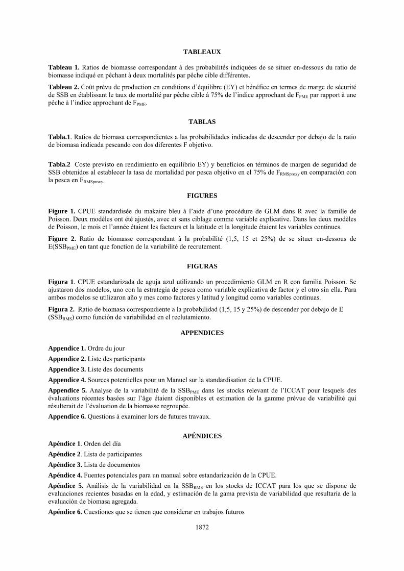
1872

TABLEAUX

Tableau 1. Ratios de biomasse correspondant à des probabilités indiquées de se situer en-dessous du ratio de biomasse indiqué en pêchant à deux mortalités par pêche cible différentes.

Tableau 2. Coût prévu de production en conditions d’équilibre (EY) et bénéfice en termes de marge de sécurité de SSB en établissant le taux de mortalité par pêche cible à 75% de l’indice approchant de FPME par rapport à une pêche à l’indice approchant de FPME.

TABLAS

Tabla.1. Ratios de biomasa correspondientes a las probabilidades indicadas de descender por debajo de la ratio de biomasa indicada pescando con dos diferentes F objetivo.

Tabla.2 Coste previsto en rendimiento en equilibrio EY) y beneficios en términos de margen de seguridad de SSB obtenidos al establecer la tasa de mortalidad por pesca objetivo en el 75% de FRMSproxy en comparación con la pesca en FRMSproxy.

FIGURES

Figure 1. CPUE standardisée du makaire bleu à l’aide d’une procédure de GLM dans R avec la famille de Poisson. Deux modèles ont été ajustés, avec et sans ciblage comme variable explicative. Dans les deux modèles de Poisson, le mois et l’année étaient les facteurs et la latitude et la longitude étaient les variables continues.

Figure 2. Ratio de biomasse correspondant à la probabilité (1,5, 15 et 25%) de se situer en-dessous de E(SSBPME) en tant que fonction de la variabilité de recrutement.

FIGURAS

Figura 1. CPUE estandarizada de aguja azul utilizando un procedimiento GLM en R con familia Poisson. Se ajustaron dos modelos, uno con la estrategia de pesca como variable explicativa de factor y el otro sin ella. Para ambos modelos se utilizaron año y mes como factores y latitud y longitud como variables continuas.

Figura 2. Ratio de biomasa correspondiente a la probabilidad (1,5, 15 y 25%) de descender por debajo de E (SSBRMS) como función de variabilidad en el reclutamiento.

APPENDICES

Appendice 1. Ordre du jour

Appendice 2. Liste des participants

Appendice 3. Liste des documents

Appendice 4. Sources potentielles pour un Manuel sur la standardisation de la CPUE.

Appendice 5. Analyse de la variabilité de la SSBPME dans les stocks relevant de l’ICCAT pour lesquels des évaluations récentes basées sur l’âge étaient disponibles et estimation de la gamme prévue de variabilité qui résulterait de l’évaluation de la biomasse regroupée.

Appendice 6. Questions à examiner lors de futures travaux.

APÉNDICES

Apéndice 1. Orden del día

Apéndice 2. Lista de participantes

Apéndice 3. Lista de documentos

Apéndice 4. Fuentes potenciales para un manual sobre estandarización de la CPUE.

Apéndice 5. Análisis de la variabilidad en la SSBRMS en los stocks de ICCAT para los que se dispone de evaluaciones recientes basadas en la edad, y estimación de la gama prevista de variabilidad que resultaría de la evaluación de biomasa agregada.

Apéndice 6. Cuestiones que se tienen que considerar en trabajos futuros

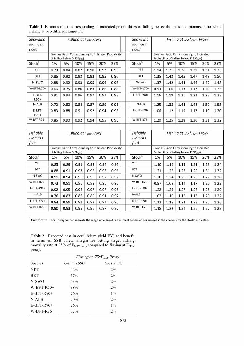
1873

1

Entries with –Rxx+ designations indicate the range of years of recruitment estimates considered in the analysis for the stocks indicated.

Table 2. Expected cost in equilibrium yield EY) and benefit in terms of SSB safety margin for setting target fishing mortality rate at 75% of FMSY proxy compared to fishing at FMSY proxy.

Fishing at .75*FMSY Proxy

Species Gain in SSB Loss in EY

YFT 42% 2%

BET 57% 2%

N-SWO 53% 2%

W-BFT-R70+ 38% 2%

E-BFT-R90+ 26% 1%

N-ALB 70% 2%

E-BFT-R70+ 26% 1%

W-BFT-R76+ 37% 2%

Table 1. Biomass ratios corresponding to indicated probabilities of falling below the indicated biomass ratio while fishing at two different target Fs.

Spawning Biomass (SSB)

Fishing at FMSY Proxy Spawning Biomass (SSB)


Biomass Ratio Corresponding to Indicated Probability of falling below E(SSBMSY)

Biomass Ratio Corresponding to Indicated Probability of falling below E(SSBMSY)

Stock1 1% 5% 10% 15% 20% 25% Stock1 1% 5% 10% 15% 20% 25%

YFT 0.79 0.84 0.87 0.90 0.92 0.93 YFT 1.14 1.21 1.26 1.29 1.31 1.33

BET 0.86 0.90 0.92 0.93 0.95 0.96 BET 1.35 1.42 1.45 1.47 1.49 1.50

N‐SWO 0.88 0.92 0.93 0.95 0.96 0.96 N‐SWO 1.37 1.42 1.44 1.46 1.47 1.48

W‐BFT‐R70+ 0.66 0.75 0.80 0.83 0.86 0.88 W‐BFT‐R70+ 0.93 1.06 1.13 1.17 1.20 1.23

E‐BFT‐R90+

0.91 0.94 0.96 0.97 0.97 0.98 E‐BFT‐R90+ 1.16 1.19 1.21 1.22 1.23 1.23

N‐ALB 0.72 0.80 0.84 0.87 0.89 0.91 N‐ALB 1.25 1.38 1.44 1.48 1.52 1.55

E‐BFT‐R70+

0.83 0.88 0.91 0.92 0.94 0.95 E‐BFT‐R70+ 1.06 1.12 1.15 1.17 1.19 1.20

W‐BFT‐R76+ 0.86 0.90 0.92 0.94 0.95 0.96 W‐BFT‐R76+ 1.20 1.25 1.28 1.30 1.31 1.32

Fishable Biomass (FB)

Fishing at FMSY Proxy Fishable Biomass (FB)


Biomass Ratio Corresponding to Indicated Probability of falling below E(FBMSY)

Biomass Ratio Corresponding to Indicated Probability of falling below E(FBMSY)

Stock1 1% 5% 10% 15% 20% 25% Stock1 1% 5% 10% 15% 20% 25%

YFT 0.85 0.89 0.91 0.93 0.94 0.95 YFT 1.10 1.16 1.19 1.21 1.23 1.24 BET 0.88 0.91 0.93 0.95 0.96 0.96 BET 1.21 1.25 1.28 1.29 1.31 1.32

N‐SWO 0.91 0.94 0.95 0.96 0.97 0.97 N‐SWO 1.20 1.24 1.25 1.26 1.27 1.28 W‐BFT‐R70+ 0.73 0.81 0.86 0.89 0.90 0.92 W‐BFT‐R70+ 0.97 1.08 1.14 1.17 1.20 1.22 E‐BFT‐R90+ 0.92 0.95 0.96 0.97 0.97 0.98 E‐BFT‐R90+ 1.22 1.25 1.27 1.28 1.28 1.29

N‐ALB 0.76 0.83 0.86 0.89 0.91 0.92 N‐ALB 1.02 1.10 1.15 1.18 1.20 1.22 E‐BFT‐R70+ 0.84 0.89 0.91 0.93 0.94 0.95 E‐BFT‐R70+ 1.12 1.18 1.21 1.23 1.25 1.26 W‐BFT‐R76+ 0.90 0.93 0.95 0.96 0.97 0.97 W‐BFT‐R76+ 1.18 1.22 1.24 1.26 1.27 1.28

1874

Figure 1. Standardized blue marlin CPUE using GLM procedure in R with the Poisson family. Two models were fit, with and without target as a factor explanatory variable. Both Poisson models had month and year as factors and latitude and longitude as continuous variables.

0.5

0.6

0.7

0.8

0.9

1.0

0.0 0.2 0.4 0.6 0.8 1.0

SS

B/S

SB

Fm

ax

recruitment CV

1%

0.50

0.60

0.70

0.80

0.90

1.00

0.00 0.20 0.40 0.60 0.80 1.00

SS

B/S

SB

Fm

ax

recruitment CV

5%

0.5

0.6

0.7

0.8

0.9

1.0

0.0 0.2 0.4 0.6 0.8 1.0

SS

B/S

SB

Fm

ax

recruitment CV

15%

0.5

0.6

0.7

0.8

0.9

1.0

0.0 0.2 0.4 0.6 0.8 1.0

SS

B/S

SB

Fm

ax

recruitment CV

25%

Figure 2. Biomass ratio corresponding to probability (1.5, 15 and 25%) of falling below E(SSBMSY) as a function of the recruitment variability.

1875

Appendix 1

AGENDA 1. Opening, adoption of the Agenda and meeting arrangements. 2. Manual for CPUE standardization 3. Review of methods to address species targeting and gear/species overlap during CPUE standardization 4. Influence of life history characteristics, environmental variability and gear selectivity on Status

Determination with respect to the Convention objectives 5. Other matters 6. Recommendations 7. Adoption of the report and closure

Appendix 2

LIST OF PARTICIPANTS

SCRS CHAIRMAN Scott, Gerald P. SCRS Chairman, NOAA Fisheries, Southeast Fisheries Science Center Sustainable Fisheries Division, 75 Virginia Beach Drive, Miami, Florida 33149 Tel: +1 305 361 4261, Fax: +1 305 361 4219, E-Mail: [email protected] CONTRACTING PARTIES BRAZIL Minte-Vera, Carolina V. Universidade Estadual de Maringá, Av. Colombo, nº 5790 - Bloco H90, Mirangá, PR Tel: +55 44 3261 4622, Fax: , E-Mail: [email protected] CANADA Neilson, John D. Head, Large Pelagics Projects, Population Ecology Section, St. Andrews Biological Station, Fisheries and Oceans, Canada, 531 Brandy Cove Road, St. Andrews, New Brunswick Tel: +1 506 529 4922, Fax: +1 506 529 5862, E-Mail: [email protected] EUROPEAN COMMUNITY Abascal Crespo, Francisco Javier Instituto Español de Oceanografía, Centro Oceanográfico de Canarias, Apdo. Correos 1373, 38005 Santa Cruz de Tenerife, Spain Tel: +34 922 549 400, Fax: +34 922 549 554, E-Mail: [email protected] De Bruyn, Paul AZTI - Tecnalia, Herrera Kaia Portualdea z/g, 20110 Pasaia, Gipuzkoa, Spain Tel: +34 943 004800, Fax: +34 943 004801, E-Mail: [email protected] Di Natale, Antonio Director-AQUASTUDIO, Via Trapani, nº 6, 98121, Messina, Sicilia, Italy Tel: +39 090 346 408, Fax: +39 090 364 560, E-Mail: [email protected] Gaertner, Daniel I.R.D. UR nº 109 Centre de Recherche Halieutique Méditerranéenne et Tropicale, , Avenue Jean Monnet - B.P. 171, 34203, Sète Cedex, France Tel: +33 4 99 57 32 31, Fax: +33 4 99 57 32 95, E-Mail: [email protected] Ortiz de Urbina, Jose Maria Instituto Español de Oceanografía, C.O de Málaga, , Apartado 285 - Puerto Pesquero s/n, 29640, Fuengirola, Málaga, Spain Tel: +34 952 47 1907, Fax: +34 952 463 808, E-Mail: [email protected]

1876

Ortiz de Zárate Vidal, Victoria Ministerio de Educación y Ciencia, Instituto Español de Oceanografía, Promontorio de San Martín s/n, 39012, Santander, Cantabria, Spain Tel: +34 942 29 10 60, Fax: +34 942 27 50 72, E-Mail: [email protected] Pereira, Joao Gil Universidade dos Açores, Departamento de Oceanografia e Pescas, 9900 Horta, Portugal Tel: +351 292 200 431, Fax: +351 292 200 411, E-Mail: [email protected] Rodríguez-Marín, Enrique Instituto Español de Oceanografía, C.O. de Santander, Promontorio de San Martín s/n, 39004 Santander, Cantabria, Spain Tel: +34 942 29 10 60, Fax: +34 942 27 50 72, E-Mail: [email protected] JAPAN Takeuchi, Yukio National Research Institute of Far Seas Fisheries, Fisheries Research Agency of Japan, Mathematical Bilogy Section- Pelagic Resource Division, 7-1, 5 Chome Orido, Shizuoka-Shi, Shimizu-ku Tel: +81 543 36 6039, Fax: +81 543 35 9642, E-Mail: [email protected] MOROCCO Idrissi, M'Hammed Chef, Centre Régional de l'INRH á Tanger, , B.P. 5268, 90000, Drabeb, Tanger Tel: +212 39 325 134, Fax: +212 39 325 139, E-Mail: [email protected];[email protected] TURKEY Karakulak, Saadet Faculty of Fisheries, Istanbul University, Ordu Cad. Nº 200, 34470, Laleli, Istanbul Tel: +90 212 455 5700/16418, Fax: +90 212 514 0379, E-Mail: [email protected] UNITED STATES Cass-Calay, Shannon NOAA Fisheries, Southeast Fisheries Center, Sustainable Fisheries Division, 75 Virginia Beach Drive, Miami, Florida 33149 Tel: +1 305 361 4231, Fax: +1 305 361 4562, E-Mail: [email protected] Goodyear, Phil 1214 North Lakeshore Drive, Niceville, Florida 32518 Tel: +1 850 897 2666, Fax: +1 850897 2666, E-Mail: [email protected] Schirripa, Michael NOAA Fisheries, Southeast Fisheries Science Center, 75 Virginia Beach Drive, Miami, Florida 33149 Tel: +1 305 361 4288, Fax: +1 305 361 4562, E-Mail: [email protected]

OBSERVERS Non-governmental Organizations Federacion of European Aquaculture Producers-FEAP Caruana, Saviour Tarxien Road, Ghaxaq, MALTA Tel: +356 2180 9460, Fax: +356 2180 9462, E-Mail:[email protected]

**********

ICCAT SECRETARIAT C/Corazón de María, 8 – 6º planta; 28002 Madrid, Spain

Tel: +3491 416 5600; Fax: +3491 415 2612; E-Mail: [email protected]

Restrepo, Víctor Pallarés, Pilar

1877

Appendix 3

LIST OF DOCUMENTS

SCRS/2009/027 Conveying the overall situation of the ICCAT stocks through the use of face plots. Schirripa,

M.J. and V. R. Restrepo SCRS/2009/028 CPUE standardizations of species targeting in longline fisheries: initial investigations of the

utility of simulated data for method verification. Schirripa, M.J. and C. P. Goodyear SCRS/2009/029 Evaluating the efficacy of minimum stock size thresholds in the presence of natural

variability and parameter uncertainty: an application to northern albacore tuna (Thunnus alalunga). Ortiz, M., S. L. Cass-Calay and G. P. Scott

SCRS/2009/030 Common trends model in catch per unit of effort for the tropical tunas. Gaertner, D. SCRS/2009/031 An exploration of targeting variables in the Canadian swordfish longline CPUE. Stacey D.

Paul and John D. Neilson

Appendix 4

INPUTS TO THE STANDARDIZATION OF CATCH AND EFFORT DATA FROM FISHERY-DEPENDENT SOURCES TO USE AS RELATIVE INDEX OF ABUNDANCE MANUAL

MODEL DIAGNOSTICS (Section provided by M. Ortiz)

The common practice of model fitting involves the selection of a model class appropriate to the data, fitting and results presentation. Comparisons between alternative models are normally related to “goodness” of fit to the data, and the selected model is commonly ‘the best fit’ according to some specific criteria, such as log likelihood, AIC or similar statistics. However, seldom there is a report of the model diagnostics and evaluation of “appropriateness” of the model implicit assumptions to the data structure. Selection of the model class is usually the first step and decisions should take into account the nature of the data and objective(s) of the analysis mainly. But, even after a “proper” selection of the class model, the data themselves may show inconsistencies in the fitting process. These inconsistencies can arise from: a) the data as whole show systematic departures of the model assumptions, and or b) that a subset of observations shows discrepancies from the rest of the data. Therefore model checking should be an integral part of the model fitting. Based on diagnostics the modeler will introduce a verification step in the process assuring that the selected model is the appropriate one given the data analyzed. McCullagh and Nelder (1989) classified the model checking techniques into two groups: a) informal, those that relay on subjective human decision to determine patterns or better, departure from expected patterns. And b) formal techniques that imply a wider model (where the “selected current model” is a subset) with higher number of parameters. In this case, the current model passes the check if it can demonstrate that the extra parameter(s) in the wider model did not improve the fitting of the data.

Model checking elements

Model checking was originally developed for classical linear models, then McCullagh and Nelder (1989) extended it to Generalized Linear Models (GLMs). Analysis of residuals are the primarily element for model checking, however other components in model checking include the fitted values, the linear predictors, the residual variance, the dispersion parameter and the elements of the projection (‘hat’) matrix. The classical residual definition; r = y – µ is often called “response residual” in GLMs (R, S-Plus, SAS) and is simply the difference between the observed value and the corresponding predicted by the model. Depending upon the GLM error model distribution, residuals are often transformed such its variance is constant and have a “normal like” behavior for model checking purposes, these residuals are called “standardized residuals” and include: i) the “Pearson residuals”, where response residuals are scaled by the estimated standard deviation of the

1882

EXAMPLE OF A REPORT CARD FOR EVALUATION OF ALTERNATIVE INDICES OF ABUNDANCE. FROM SEDAR-CPUE WORKSHOP MIAMI NOV-2008. (Provided by S. Cass-Calay)

DESCRIPTION OF THE DATA SOURCE

1. Fishery Independent Indices No

t A

pp

licab

le

Ab

sen

t

Inco

mp

lete

Co

mp

lete

Working Group Comments:

A. Describe the survey design (e.g. fixed sampling sites, random stratified sampling), location, seasons/months and years of sampling.

B. Describe sampling methodology (e.g. gear, vessel, soak time etc.)

C. Describe any changes in sampling methodology (e.g. gear, vessel, sample design etc.)

D. Describe the variables reported in the data set (e.g. location, time, temperature, catch, effort etc.).

E. What species or species assemblages are targeted by this survey (e.g. red snapper, reef fish, pelagic).

F. Describe the size/age range that the index applies to. Include supporting figures (e.g. size comp) if available.

2. Fishery Dependent Indices

A. Describe the data source and type of fishery (e.g. commercial handline, commercial longline, recreational hook and line etc.).

B. Describe any changes to reporting requirements, variables reported, etc.

C. Describe the variables reported in the data set (e.g. location, time, temperature, catch, effort etc.).

D Describe the size/age range that the index applies to. Include supporting figures (e.g. size comp) if available.

METHODS

1. Data Reduction and Exclusions

A. Describe any data exclusions (e.g. gears, fishing modes, sampling areas etc.). Report the number of records removed and justify removal.

B. Describe data reduction techniques (if any) used to address targeting (e.g. Stephens and MacCall, 2004; gear configuration, species assemblage etc).

C. Discuss procedures used to identify outliers. How many were identified? Were they excluded?

1883

2. Management Regulations (for FD Indices) No

t A

pp

licab

le

Ab

sen

t

Inco

mp

lete

Co

mp

lete


A. Provide (or cite) history of management regulations (e.g. bag limits, size limits, trip limits, closures etc.).

B. Describe the effects (if any) of management regulations on CPUE

C. Discuss methods used (if any) to minimize the effects of management measures on the CPUE series.

3. Describe Analysis Dataset (after exclusions and other treatments)

A. Provide tables and/or figures of number of observations by factors (including year, area, etc.) and interaction terms.

B. Include tables and/or figures of number of positive observations by factors and interaction terms.

C. Include tables and/or figures of the proportion positive observations by factors and interaction terms.

D. Include tables and/or figures of average (unstandardized) CPUE by factors and interaction terms.

E. Include annual maps of locations of survey sites (or fishing trips) and associated catch rates OR supply the raw data needed to construct these maps (Observation, Year, Latitude, Longitude (or statistical grid, area), Catch, Effort).

F. Describe the effort variable and the units. If more than one effort variable is present in the dataset, justify selection.

G. What are the units of catch (e.g. numbers or biomass, whole weight, gutted weight, kilograms, pounds).

4. Model Standardization

A. Describe model structure (e.g. delta-lognormal)

B. Describe construction of GLM components (e.g. forward selection from null etc.)

C. Describe inclusion criteria for factors and interactions terms.

D. Were YEAR*FACTOR interactions included in the model? If so, how (e.g. fixed effect, random effect)? Were random effects tested for significance using a likelihood ratio test?

E. Provide a table summarizing the construction of the GLM components.

F. Summarize model statistics of the mixed model formulation(s) (e.g. log likelihood, AIC, BIC etc.)

G. Report convergence statistics.

1884

MODEL DIAGNOSTICS Comment: Other model structures are possible and acceptable. Please provide appropriate diagnostics to the CPUE indices working group. 1. Binomial Component N

ot

A

pp

licab

le

Ab

sen

t

Inco

mp

lete

Co

mp

lete


A. Include plots of the chi-square residuals by factor.

B. Include plots of predicted and observed proportion of positive trips by year and factor (e.g. year*area)

C. Report overdispersion parameter and other fit statistics (e.g. chi-square / degrees of freedom).

2. Lognormal/Gamma Component

A. Include histogram of log(CPUE) or a histogram of the residuals of the model on CPUE. Overlay the expected distribution.

B. Include plots describing error distribution (e.g. Studentized residuals vs. linear predictor.

C. Include QQ-plot – (e.g. Student deviance residuals vs. theoretical quantiles), Overlay expected distribution.

D. Include diagnostic plot for variance function (e.g. square root of std residuals vs. fitted values). Overlay expected distribution.

E. Include diagnostic plot for link function (e.g. linear response variable vs. linear predictor). Overlay expected distribution.

F. Include plots of the residuals by factor

3. Poisson Component

A. Report overdispersion parameter and other fit statistics (e.g. chi-square / degrees of freedom).

B. Include plots describing error distribution (e.g. Studentized residuals vs. linear predictor.

C. Include QQ-plot – (e.g. Student deviance residuals vs. theoretical quantiles), Overlay expected distribution.



The feasibility of this diagnostic is still under review.

4. Zero-inflated model

A. Include ROC curve to quantify goodness of fit.

B. Include plots describing error distribution (e.g. Studentized residuals vs. linear predictor).

C. Include QQ-plot (e.g. Student dev. residuals vs. theoretical quantiles), Overlay expected distribution.

1885

MODEL DIAGNOSTIC (CONT.)

No

t A

pp

licab

le

Ab

sen

t

Inco

mp

lete

Co

mp

lete




IF MULTIPLE MODEL STRUCTURES WERE CONSIDERED:

(Note: this is always recommended but required when model diagnostics are poor.)

1. Plot of resulting indices and estimates of variance

2. Table of model statistics (e.g. AIC criteria)

Date Received

Workshop Recommendation

Revision Deadline Author and Rapporteur Signatures

First Submission

Revision

Justification of Working Group Recommendation

1886

REVIEW OF INDEX WEIGHTING SCHEMES FOR STOCK ASSESSMENTS. (Section provided by C. Porch) Stock assessment algorithms typically incorporate data on stock structure and mortality from a variety of sources including landings, length or age composition, and indices of relative abundance derived from fishery catches or fishery-independent surveys. Usually some data sets are less informative (more uncertain) than others and an important part of the stock assessment process is to determine how to take these differences into account. For example, one may wish to place greater emphasis on a large sample from the entire study population than on a small sample from a fraction of the study population. The challenge, of course, lies in objectively determining the degree to which each data source should be emphasized (weighted). At present, there is no universally accepted method for meeting this challenge, with the predictable result that the choice of weighting schemes often depends as much on who is participating in the assessment as it does on the types of data involved. As this has long been a contentious issue in many forums (Schnute and Hilborn 1993; ICCAT 1999), it is important for SEDAR participants to understand the strengths and weaknesses of the various weighting schemes before adopting one for a particular assessment. To that end, the chapter reviews the weighting schemes that have been developed specifically for indices of abundance and suggests criteria for selecting between those schemes during SEDAR data and assessment workshops. Measuring uncertainty Uncertainty can be thought of in terms of observation errors (degree to which the observed value of an index differs from its true value) and process errors (degree to which the true value of an index differs from that of the study population). Observation errors arise due to incomplete or nonrandom sampling and are typically a function of sample size. Process errors arise, for example, when the fraction of the study population that occupies the area sampled for the index varies through time. If these errors are effectively random over the study period, then one may consider them to be unbiased representations of the study population (although they may still be highly imprecise). In that case it is advantageous to have multiple indices representing the same quantity or, when possible, to combine several uncertain indices into one (see Conn’s chapter). Systematic observation or process errors, of course, can lead to bias. Known biases of a substantive nature should obviously be corrected during the index standardization process or else the index should be discarded. The relevant question here is what to do with indices that are suspected of some unknown bias. In many assessments the available data are too sparse to afford the luxury of simply discarding suspicious indices. For such cases, we maintain that unknown biases among multiple independent data sets may be regarded (hopefully) as canceling out on average and therefore may be treated as another degree of imprecision. It is therefore appropriate simply to deemphasize such data during the fitting process in some proportion to the degree to which bias is suspected (more on this later). Given these caveats, the next order of business is to select a common metric for measuring the uncertainty of each candidate index of abundance. Most modern stock assessment models are cast in a probabilistic framework, in which case the most natural measure of the uncertainty in an index is its variance. For example, consider two independent normally distributed indices X1 and X2 with the same expectation but different variances (

2 and 2). The probability of

observing two given values x1 and x2 is

(1)

22

22

21

21

2121 2

)(

2

)(exp

2

1),(

xx

xxp

The maximum likelihood estimator for is the value that maximizes equation 1, or equivalently, minimizes its negative logarithm:

(2) 22

22

21

21

2121 2

)(

2

)()2ln(),(ln

xx

xxp

The solution when 1 and 2 are known is easily obtained by simple calculus:

1887

(3)

22

21

22

221

1 11ˆ

xx

As can be seen, the influence of each index series on the final estimate of is directly proportional to the variance associated with that index. Some authors have adopted somewhat simpler notation where weight coefficients (w) are specified directly in the likelihood function, e.g.,

(4) 2

222

1121 )()(),(ln xwxwxxp In this example it is easy to see that the w’s are merely the reciprocals of the variances and that minimizing (4) or (2) will yield identical results as long as the variances (and w’s) are constant. In keeping with most statistical texts, we find the variance notation to be more intuitive, particularly when different error structures are mixed such that the relative values of the w coefficients are no longer comparable. Moreover, the weighting coefficient formulation is impractical when the values of the weights are to be estimated internally in the model. Review of index weighting schemes The weights applied to the indices of abundance used can have a profound effect on the outcome of an assessment. To illustrate this, consider the following simple model:

(5) tt

tt

GtNqx

GtNqx

,22,2

,11,1

)(

)(

where x1,t and x2,t are values of independent indices representing an underlying population that is growing linearly with time t from a known starting abundance (N). If the errors and are approximately normal-distributed with equal variances, then maximum likelihood estimates for q1, q2, and G may be obtained by minimizing

(6) 2

22,2

2

21,12

21 2

))((

2

))(()2ln(),(ln

GtNqxGtNqxxxp tt

t

Otherwise, the appropriate likelihood function for unequal variances is

(7) 22

22,2

21

21,1

2121 2

))((

2

))(()2ln(),(ln

GtNqxGtNqxxxp tt

t

In both (6) and (7) the over-arrow denotes the vector of time series observations for each index. It is easy to show that the estimates for q1, q2, and G obtained from the equal variance formulation (6) will be the same whether 2 is estimated or fixed to an arbitrary constant (which is the least squares solution). It is also generally true that the equal-variance (6) and bi-variance (7) estimators will perform similarly when applied to situations where the true variances of each index are the same (and the underlying model is correct). However, if the true variances are substantially different, the assumption of equal variances (application of 6) can lead to biased estimates. Figure 1a and Table 1 compare the results when the equal-variance (6) and bi-variance (7) estimators were applied to simulated indices generated according to (5) when the true values of

2 and 2 were set to 64 and 13,

respectively. The bi-variance estimator performed best, producing slightly better parameter estimates and a much lower value for the likelihood function. This would seem to confirm that there is some advantage to estimating separate variances for each index rather than assuming they are the same, however the experiment was predicated on having the correct underlying model. Consider now the same set of experiments when the indices of abundance were equally biased, but in opposite directions such that the annual rate of increase for index 1 is 0.2 and the annual rate for index 2 is 1.8 (compared to the true rate of 1.0). In that case the bi-variance estimator

1888

again produced a significantly lower likelihood function value than the equal-variance estimator (82.6 versus 96.6), and on that basis an investigator might be tempted to prefer it. However, closer inspection reveals that the bi-variance estimator produced this low likelihood value by severely down-weighting the less precise index 1 and focusing on the more precise index 2 (Figure 1b). As a result, the MLEs for q2 and

2 were very close to the true values and the predicted values for index 2 matched the observations very well, whereas the MLE for

2 was double the true value and the predicted values for index 1 did not match the observations at all. Hence, the estimate of the primary parameter of interest (G) was 1.8; matching the true slope of index 2, but much higher than the underlying population. In contrast, the equal variance estimator gave equal credence to the two biased indicators and essentially averaged them, in this case resulting in a much less biased estimate of G.

Table 1. Parameter estimates from the equal-variance and bi-variance estimators applied to data generated from model 5.

Unbiased indices Conflicting indices Parameter TRUE Equal-var. Bi-variance Equal-var. Bi-variance G 1 0.98 1.01 1.11 1.81 q1 2 2.04 1.99 0.57 0.37 q2 1 1.02 0.99 1.54 1 1

2 64 46 64 76 111 2

2 13 46 13 76 13

The above example above was contrived to make the points that (1) weighting matters and (2) the estimation of variances is inextricably linked to the assumption that the model underlying the estimator is correct. While one variance scheme may appear better on the basis of the values of the likelihood function or other metric, it may in fact exacerbate potential biases by favoring solutions which disregard indices that are difficult to reconcile with the model but nevertheless accurate. For this, and other reasons that will become apparent, there is no widely accepted protocol for choosing a weighting scheme. Therefore it behooves the analyst to be familiar with both the indices being used and with the strengths and weaknesses of the various weighting options. The remaining discussion presents six basic approaches to index weighting. Most of the weighting schemes developed to date are essentially special cases of these six categories. The implementation of each scheme depends, of course, on the type of error structure assumed. The normal and lognormal error structures seem to be the most common choices in the literature; the latter in particular because it places less weight on outliers and because the variance of many indices tends to increase with the mean. Other error structures (e.g., gamma, Poisson, negative binomial) have also been considered, but the basic principles are the same. For the sake of brevity, equations are shown only for the normal and lognormal cases. Equal Weighting.- The simplest weighting scheme is the so-called “equal weighting” option, where all observations are essentially assigned the same variance (i.e., all indices j in all years y) so that the likelihood function has the form:

(8)

normalx

normalx

L

xyj x

yjyj

yj

yjyj

logln2

)(ln

ln2

)(

ln,

2ln

2,,

,2

2,,

Note that is the expectation in the case of the normal distribution and the median in the case of the lognormal distribution. Also, the variance term in the normal case is on an arithmetic scale whereas in the lognormal case it is on a logarithmic scale (i.e., the variance of ln x ). Hence, the implications of equal weighting are somewhat different between the two error structures; constant variance in the normal case and constant coefficient of

variation (CV) in the lognormal case (recall 2ln x = ln(1+CV2) ). It is also important to note that in the case of a

normal distribution, the annual values for each index should be rescaled so that their means are similar (e.g., by dividing the original series by their respective means), otherwise series with larger absolute values will receive more weight in the fitting process than series with low values. In the lognormal case the scaling is implicit and the results will be the same whether the series is rescaled or not. In equal-weighting models where the uncertainty is limited to the indices of abundance (e.g., catch is assumed known without error), the estimates of will not depend on the value of the variance parameter (or whether it is estimated or not), but will depend on

1889

the choice between lognormal and normal errors. Simple maximum likelihood weighting.- A simple extension of the equal weighting procedure is to assume the variance parameter for a given index is constant from year to year, but may differ among indices:

(9)

lognormalx

normalx

L

jxyj jx

yjyj

jyj j

yjyj

,ln,

2,ln

2,,

,2

2,,

ln2

)(ln

ln2

)(

In this case the variance parameters may be fixed to some externally derived values (a special case of input variance weighting discussed below) or estimated internally in the model. Maximum likelihood estimates of the variances have been derived in three common ways. An early method was referred to as iterative re-weighting because it consisted of a two step process where the likelihood was minimized using fixed values for each variance parameter, after which the variances were recomputed using the standard MLEs.

(10)

normalxn

normalxn

yyjyjjx

yyjyjj

log)(ln1

)(1

2,,,ln

2,,

2

The new estimates of variance would be substituted back into the likelihood and the minimization procedure reinitiated until the estimates of variance converged (essentially an application of the EM algorithm). Subsequently, it was realized that the concentrated likelihood approach, whereby the formulas in (10) are directly substituted into (9), was more efficient and yielded the same results. Alternatively, equivalent MLEs may be obtained by use of the search algorithm (minimizing 9) in the same manner as for the other estimated parameters (Porch 2002). Note that annual variances cannot be estimated using these techniques because the number of index parameters would exceed the number of index data points. One potential pitfall of simple maximum likelihood weighting is that some index series may be severely down-weighted, as illustrated in the example. This is especially problematic if the assessment model is mis-specified and happens to match up (incorrectly) with some indices more than others. Simulations by Legault and Porch (2001) that were conditioned on data for Atlantic bluefin tuna (with various minor model mis-specifications) indicated no clear pattern in the bias or uncertainty of estimates between the equal weighting and maximum likelihood schemes. Input-variance weighting.- This common alternative to equal weighting simply involves specifying the variance parameters based on considerations external to the stock assessment model. For example, estimates of the variance of an index may be derived for each year during the standardization process (e.g., by application of a general linear model). To the extent that they are reasonable estimates of year to year changes in index uncertainty, incorporating such externally derived variances can lead to more accurate assessments (Maunder and Starr 2003).

(11)

normalx

normalx

L

yjxyj yjx

yjyj

yjyj yj

yjyj

logln2

)(ln

ln2

)(

,,ln,

2,,ln

2,,

,,

2,

2,,

Note that, in principle, it is possible to estimate the annual variance parameters for each index if the standardization procedure is conducted simultaneously with the stock assessment (Maunder 2001). In practice, however, the process is prohibitively time consuming. Some scientists have advocated developing input weights based entirely on expert opinion, arguing that issues such as spatial coverage and potential for bias outweigh consideration of observation error. For example, Suzuki

1890

(2001) presented a framework where indices for bluefin tuna would be graded (on a scale of 1 to 5) on each of three factors: spatial coverage, temporal coverage, and the likely importance of changes in the operational characteristics of the index over time that are not accounted for during the index standardization process. Each index would then be weighted in accordance with the sum of those three scores (i.e., the variances would be set equal to the reciprocal of those scores). Additional-variance weighting.- This alternative is based on the premise that the variance of an index may be decomposed into a component reflecting observation errors, such as might be obtained from the GLM standardization, and an additional component characterizing the uncertainty in the index as a reflection of the true abundance trends, as might occur when the proportion of the stock sampled by the index varies from year to year (Wade 1996, Punt et al. 1997, Geromont and Butterworth 2001). To the extent that these two error sources are independent, one might expect their variances to be additive:

(12)

normalx

normalx

L

jyjxyj jyjx

yjyj

jyjyj jyj

yjyj

log)ln()(

)(ln

2

1

)ln()(

)(

2

1

22,,ln

,22

,,ln

2,,

22,

,22

,

2,,

where j

2 is the additional variance term which may vary among indices and can be estimated by maximum likelihood methods analogous to those discussed in connection with simple maximum likelihood weighting (equations 9 and 10). This method mitigates the pitfalls of equal weighting (e.g., giving equal credence to observations based on little data) and simple maximum likelihood weighting (e.g., all of the weight going to a few series), but still depends on the relative consistency of each series with the underlying model structure. The approach would be undesirable if there were strong a priori reasons for weighting one series more highly than another and there was uncertainty about model structure. Multiplicative-variance weighting.- This approach is similar to the additional variance approach above except that the scaling parameter is multiplied by the year-specific input values rather than added to it: .

(13)

normalcc

x

normalcc

x

L

yjxjyj yjxj

yjyj

yjjyj yjj

yjyj

log)ln()(ln

2

1

)ln()(

2

1

2,,ln

,2

,,ln

2,,

2,

,2,

2,,

In many applications the year-specific variances are initially determined by GLM and then the multiplicative parameters cj are adjusted to account for expert judgments on key factors not accounted for in the GLM (see Quinn and Deriso 1999; Sullivan et al. 1999; 2002). In the most recent assessment of Atlantic and Gulf king mackerel, for example, the cj values were adjusted such that the average coefficient of variation (CV) attributed to each index was the same, but the relative year to year changes in CV from the GLM were preserved (Cass-Calay et al., 2008). The multiplicative-variance weighting approach is perhaps less intuitive than the additional variance approach in terms of distinguishing process and observation errors. It is useful, however, for cases where the available estimates of observation variance (j,y) are trusted as measures of relative precision from one year to the next, but not as measures of the uncertainty across indices. It is of course also possible to estimate the cj values analogous to the simple maximum likelihood method, subject to the same limitations (most notably that some indices may be severely down-weighted, particularly if the assessment model is mis-specified). Variance as a function of the mean.- This last approach is based on the premise that the variance of catch per unit effort (or survey counts) tends to be correlated with the mean.

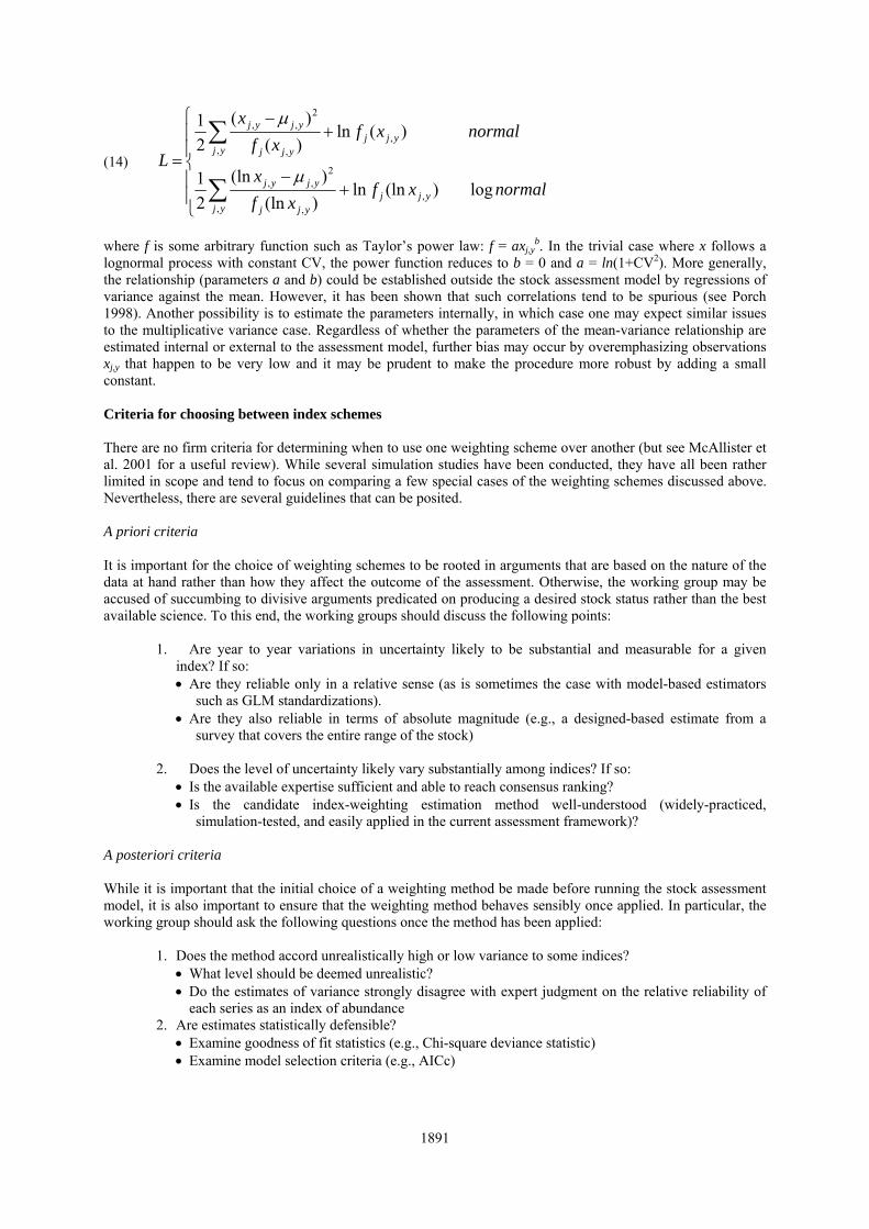
1891

(14)

normalxfxf

x

normalxfxf

x

L

yjjyj yjj

yjyj

yjjyj yjj

yjyj

log)(lnln)(ln

)(ln

2

1

)(ln)(

)(

2

1

,, ,

2,,

,, ,

2,,

where f is some arbitrary function such as Taylor’s power law: f = axj,y

b. In the trivial case where x follows a lognormal process with constant CV, the power function reduces to b = 0 and a = ln(1+CV2). More generally, the relationship (parameters a and b) could be established outside the stock assessment model by regressions of variance against the mean. However, it has been shown that such correlations tend to be spurious (see Porch 1998). Another possibility is to estimate the parameters internally, in which case one may expect similar issues to the multiplicative variance case. Regardless of whether the parameters of the mean-variance relationship are estimated internal or external to the assessment model, further bias may occur by overemphasizing observations xj,y that happen to be very low and it may be prudent to make the procedure more robust by adding a small constant. Criteria for choosing between index schemes There are no firm criteria for determining when to use one weighting scheme over another (but see McAllister et al. 2001 for a useful review). While several simulation studies have been conducted, they have all been rather limited in scope and tend to focus on comparing a few special cases of the weighting schemes discussed above. Nevertheless, there are several guidelines that can be posited.

A priori criteria

It is important for the choice of weighting schemes to be rooted in arguments that are based on the nature of the data at hand rather than how they affect the outcome of the assessment. Otherwise, the working group may be accused of succumbing to divisive arguments predicated on producing a desired stock status rather than the best available science. To this end, the working groups should discuss the following points:

1. Are year to year variations in uncertainty likely to be substantial and measurable for a given

index? If so: Are they reliable only in a relative sense (as is sometimes the case with model-based estimators

such as GLM standardizations). Are they also reliable in terms of absolute magnitude (e.g., a designed-based estimate from a

survey that covers the entire range of the stock) 2. Does the level of uncertainty likely vary substantially among indices? If so:

Is the available expertise sufficient and able to reach consensus ranking? Is the candidate index-weighting estimation method well-understood (widely-practiced,

simulation-tested, and easily applied in the current assessment framework)?

A posteriori criteria

While it is important that the initial choice of a weighting method be made before running the stock assessment model, it is also important to ensure that the weighting method behaves sensibly once applied. In particular, the working group should ask the following questions once the method has been applied:

1. Does the method accord unrealistically high or low variance to some indices? What level should be deemed unrealistic? Do the estimates of variance strongly disagree with expert judgment on the relative reliability of

each series as an index of abundance 2. Are estimates statistically defensible?

Examine goodness of fit statistics (e.g., Chi-square deviance statistic) Examine model selection criteria (e.g., AICc)

1892

A flow chart is offered in Figure 2 to help facilitate discussions relating to the above criteria. Of course in any given application there may be gray areas. Accordingly, the recommendations offered in the flow chart are intended to be viewed as guidance rather than hard and fast rules. Acknowledgments I thank Paul Conn, Joe O’hop and Michael Prager for their helpful suggestions.

References

Cass-Calay, S., Ortiz, M., and Restrepo, V.R. 2008, Notes on the weighting of indices for the king mackerel VPA. SEDAR 16-AW-09 in: SEDAR 16 South Atlantic and Gulf of Mexico King Mackerel.

Geromont, H.F. and Butterworth, D.S. 2001, Possible extensions to the ADAPT VPA model applied to western north Atlantic bluefin tuna, addressing in particular the need to account for "additional variance". Collect. Vol. Sci. Pap. ICCAT, 52(5): 1663-1705.

ICCAT. 1999, Collective Volume of Scientific Papers. XLIX (2).

Legault, C.M. and Porch, C.E. 2001, Comparisons of index weighting schemes for tuned virtual population analyses. Collect. Vol. Sci. Pap. ICCAT, 52(5): 1729-1738.

Maunder, M.N. 2001, A general framework for integrating the standardization of catch-per-unit-effort into stock assessment models. Can. J. Fish. Aquat. Sci. 58:795−803.

Maunder, M.N. and Starr, P.J. 2003, Fitting fisheries models to standardised CPUE abundance indices. Fisheries Research 63: 43-50.

McAllister, M., Babcock, E.A., and Pikitch, E.K. 2001, Evaluating the relative merits of alternative methods to weight different time series of abundance indices in stock assessment. Collect. Vol. Sci. Pap. ICCAT, 52(3): 1094-1115.

Parma, A.M. 2002, Bayesian approaches to the analysis of uncertainty in the stock assessment of Pacific halibut. In J. M. Berkson, L.L. Kline and D.J. Orth (eds.) Incorporating uncertainty into fishery models. American Fisheries Society Symposium 27: 113-133.

Porch, C. E. 1998. Some intrinsic limitations of sample variances in stock assessment models. Pages 385-398 in Funk, F., T.J. Quinn, J. Heifetz, J.N. Ianelli, J.E. Powers, J.F. Schweigert, P.J. Sullivan, and C.I. Zhang (ed.) Fishery Stock Assessment Models. Alaska, Sea Grant College Program Report No. AK-SG-98-011997. University of Alaska Fairbanks.

Porch, C.E. 2002, VPA-2BOX Version 3.0 User’s guide. National Marine Fisheries Service, Sustainable Fisheries Division Contribution SFD-01/02-175 (also published internationally on ICCAT web page)

Punt, A.E., J.G. Cooke, D.L. Borchers, and S. Strindberg. 1997, Estimating the extent of additional variance for Southern Hemishere minke whales from the results of the IWC/IDCR cruises. Rep. int. Whal. Comm. 47:431-434.

Quinn II, T.J. and Deriso, R.B. 1999, Quantitative fish dynamics. Oxford University Press. Oxford.

Schnute, J.T. and Hilborn, R. 1993, Analysis of contradictory data sources in fish stock assessments. Can. J. Fish. Aquat. Sci. 52: 2063-2077.

Sullivan, P.J., Parma, A.M., and Clark, W.G. 1999, The Pacific halibut stock assessment of 1997. International Pacific Halibut Commission Scientific Report 79, 84 pp.

Suzuki, Z. 2001, Comparisons Qualitative evaluation of CPUE series used for West Atlantic bluefin stock assessment. Collect. Vol. Sci. Pap. ICCAT, 52(3): 977-983.

Wade, P.R. 1996, Gray whale stock assessment. Document SC/48/AS8 presented to the June 1996 meeting of the IWC Scientific Committee meeting. 17pp.

1893

(a) two unbiased indices

0

2

4

6

8

10

12

0 2 4 6 8 10 12

obs 1

obs 2

1 sigma

2 sigmas

TRUE

(b) two conflicting indices

0

2

4

6

8

10

12

14

16

18

20

0 2 4 6 8 10 12

obs 1

obs 2

1 sigma

2 sigmas

TRUE

Figure 1. Predicted trends in population growth using the equal-variance (red) and bi-variance estimators (blue) compared to the true values (diamonds) and ‘observed’ values for index 1 (circles) and index 2 (triangles). The top and bottom panels refer to the cases when the ‘observed’ values are generated without bias (Fig. 1a) or generated with equal but opposite biases (Fig. 1b).

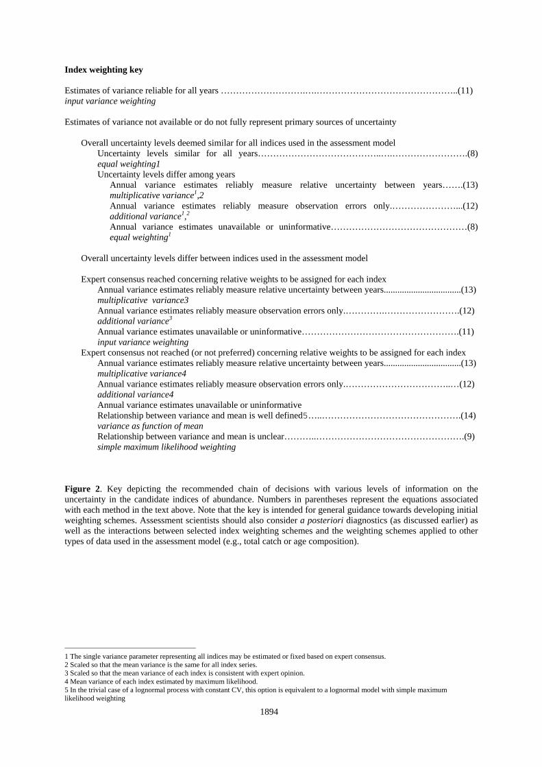
1894

Index weighting key Estimates of variance reliable for all years ……………………….….………………………………………..(11) input variance weighting Estimates of variance not available or do not fully represent primary sources of uncertainty

Overall uncertainty levels deemed similar for all indices used in the assessment model

Uncertainty levels similar for all years…………………………………..….…………………….(8) equal weighting1 Uncertainty levels differ among years

Annual variance estimates reliably measure relative uncertainty between years…….(13) multiplicative variance1,2 Annual variance estimates reliably measure observation errors only.…………………...(12) additional variance1,2

Annual variance estimates unavailable or uninformative………………………………………(8) equal weighting1

Overall uncertainty levels differ between indices used in the assessment model

Expert consensus reached concerning relative weights to be assigned for each index

Annual variance estimates reliably measure relative uncertainty between years..................................(13) multiplicative variance3 Annual variance estimates reliably measure observation errors only.………….…………………….(12) additional variance3

Annual variance estimates unavailable or uninformative…………………………………………….(11) input variance weighting

Expert consensus not reached (or not preferred) concerning relative weights to be assigned for each index Annual variance estimates reliably measure relative uncertainty between years..................................(13) multiplicative variance4 Annual variance estimates reliably measure observation errors only.……………………………..…(12) additional variance4 Annual variance estimates unavailable or uninformative Relationship between variance and mean is well defined5…..……………………………………….(14) variance as function of mean Relationship between variance and mean is unclear………..………………………………………….(9) simple maximum likelihood weighting

Figure 2. Key depicting the recommended chain of decisions with various levels of information on the uncertainty in the candidate indices of abundance. Numbers in parentheses represent the equations associated with each method in the text above. Note that the key is intended for general guidance towards developing initial weighting schemes. Assessment scientists should also consider a posteriori diagnostics (as discussed earlier) as well as the interactions between selected index weighting schemes and the weighting schemes applied to other types of data used in the assessment model (e.g., total catch or age composition).

1 The single variance parameter representing all indices may be estimated or fixed based on expert consensus. 2 Scaled so that the mean variance is the same for all index series. 3 Scaled so that the mean variance of each index is consistent with expert opinion. 4 Mean variance of each index estimated by maximum likelihood. 5 In the trivial case of a lognormal process with constant CV, this option is equivalent to a lognormal model with simple maximum likelihood weighting

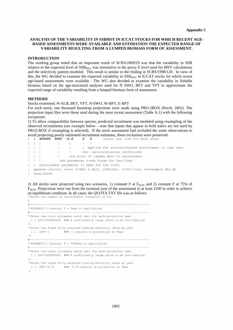
1895

Appendix 5

ANALYSIS OF THE VARIABILITY IN SSBMSY IN ICCAT STOCKS FOR WHICH RECENT AGE-BASED ASSESSMENTS WERE AVAILABLE AND ESTIMATION THE EXPECTED RANGE OF

VARIABILITY RESULTING FROM A LUMPED BIOMASS FORM OF ASSESSMENT. INTRODUCTION The working group noted that an important result of SCRS/2009/29 was that the variability in SSB relative to the expected level of SSBMSY was insensitive to the proxy F level used for MSY calculations and the selectivity pattern modeled. This result is similar to the finding in SCRS/1998/120. In view of this, the WG decided to examine the expected variability in SSBMSY in ICCAT stocks for which recent age-based assessments were available. The WG also decided to examine the variability in fishable biomass based on the age-structured analyses used for N SWO, BET and YFT to approximate the expected range of variability resulting from a lumped biomass form of assessment. METHODS Stocks examined: N-ALB, BET, YFT, N-SWO, W-BFT, E-BFT For each stock, one thousand bootstrap projections were made using PRO-2BOX (Porch, 2002). The projection input files were those used during the most recent assessment (Table A.1) with the following exceptions: 1) To allow comparability between species, predicted recruitment was modeled using resampling of the observed recruitments (see example below – note that inputs that appear in bold italics are not used by PRO2-BOX if resampling is selected). If the stock assessment had excluded the some observations to avoid projecting poorly estimated recruitment estimates, these exclusions were preserved. 1 6 400000 3500 -0.6 0 0 {enter one line for each area}

| | | | | | | | | | | | | epsilon for autocorrelated recruitment in last year | | | | | rho- autocorrelation coefficient | | | | std error of random devs in recruitment | | | ssb parameter (=ssb hinge for two-line) | | recruitment parameter (= rmax for two-line) | spawner-recruit curve (1=Bev & Holt, 2=Ricker, 3-5=2-line, 6=resample Obs R) | Zone/Stock

2) All stocks were projected using two scenarios, 1) constant F at FMAX and 2) constant F at 75% of FMAX. Projections were run from the terminal year of the assessment to at least 2100 in order to achieve an equilibrium condition. In all cases, the QUOTA.TXT file was as follows: **Enter the number of catch/effort scenarios to run 2

#------------------------------------------------------------------------- **SCENARIO 1 Constant F = Fmax to equilibrium

#------------------------------------------------------------------------- **Enter the total allowable catch (mt) for each projection year

1 1 200*1000000000 ### A sufficiently large catch to be non-limiting -1

**Enter the fixed fully-selected fishing mortality rates by year 1 1 200*-1 ### -1 results in projection at Fmax

-1 #-------------------------------------------------------------------------

**SCENARIO 2 Constant F = 75%Fmax to equilibrium #-------------------------------------------------------------------------

**Enter the total allowable catch (mt) for each projection year 1 1 200*1000000000 ### A sufficiently large catch to be non-limiting

-1 **Enter the fixed fully-selected fishing mortality rates by year

1 1 200*-0.75 ### -0.75 results in projection at Fmax -1

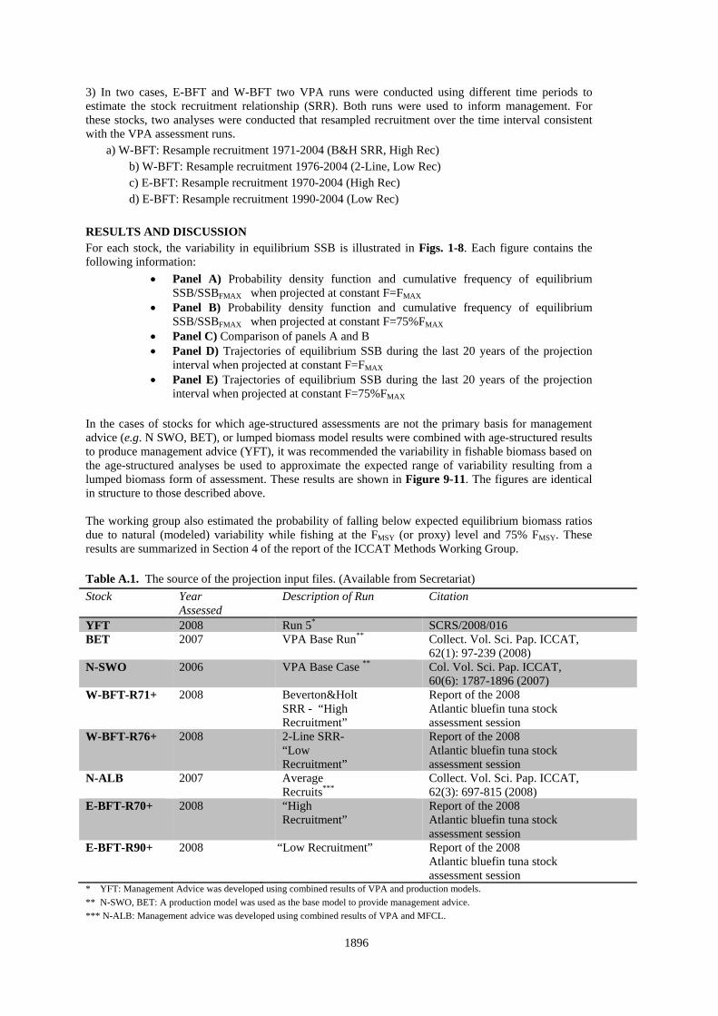
1896

3) In two cases, E-BFT and W-BFT two VPA runs were conducted using different time periods to estimate the stock recruitment relationship (SRR). Both runs were used to inform management. For these stocks, two analyses were conducted that resampled recruitment over the time interval consistent with the VPA assessment runs. a) W-BFT: Resample recruitment 1971-2004 (B&H SRR, High Rec)

b) W-BFT: Resample recruitment 1976-2004 (2-Line, Low Rec) c) E-BFT: Resample recruitment 1970-2004 (High Rec) d) E-BFT: Resample recruitment 1990-2004 (Low Rec)

RESULTS AND DISCUSSION For each stock, the variability in equilibrium SSB is illustrated in Figs. 1-8. Each figure contains the following information:

Panel A) Probability density function and cumulative frequency of equilibrium SSB/SSBFMAX when projected at constant F=FMAX

Panel B) Probability density function and cumulative frequency of equilibrium SSB/SSBFMAX when projected at constant F=75%FMAX

Panel C) Comparison of panels A and B Panel D) Trajectories of equilibrium SSB during the last 20 years of the projection

interval when projected at constant F=FMAX Panel E) Trajectories of equilibrium SSB during the last 20 years of the projection

interval when projected at constant F=75%FMAX

In the cases of stocks for which age-structured assessments are not the primary basis for management advice (e.g. N SWO, BET), or lumped biomass model results were combined with age-structured results to produce management advice (YFT), it was recommended the variability in fishable biomass based on the age-structured analyses be used to approximate the expected range of variability resulting from a lumped biomass form of assessment. These results are shown in Figure 9-11. The figures are identical in structure to those described above. The working group also estimated the probability of falling below expected equilibrium biomass ratios due to natural (modeled) variability while fishing at the FMSY (or proxy) level and 75% FMSY. These results are summarized in Section 4 of the report of the ICCAT Methods Working Group. Table A.1. The source of the projection input files. (Available from Secretariat)

Stock Year Assessed

Description of Run Citation

YFT 2008 Run 5* SCRS/2008/016 BET 2007 VPA Base Run** Collect. Vol. Sci. Pap. ICCAT,

62(1): 97-239 (2008) N-SWO 2006 VPA Base Case ** Col. Vol. Sci. Pap. ICCAT,

60(6): 1787-1896 (2007) W-BFT-R71+ 2008 Beverton&Holt

SRR - “High Recruitment”

Report of the 2008 Atlantic bluefin tuna stock assessment session

W-BFT-R76+ 2008 2-Line SRR- “Low Recruitment”


N-ALB 2007 Average Recruits***

Collect. Vol. Sci. Pap. ICCAT, 62(3): 697-815 (2008)

E-BFT-R70+ 2008 “High Recruitment”


E-BFT-R90+ 2008 “Low Recruitment” Report of the 2008 Atlantic bluefin tuna stock assessment session

* YFT: Management Advice was developed using combined results of VPA and production models.

** N-SWO, BET: A production model was used as the base model to provide management advice.

*** N-ALB: Management advice was developed using combined results of VPA and MFCL.

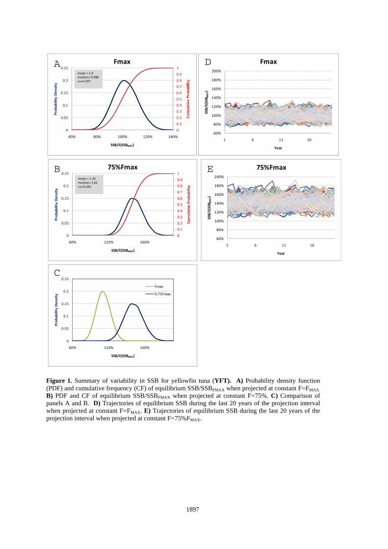
1897

Figure 1. Summary of variability in SSB for yellowfin tuna (YFT). A) Probability density function (PDF) and cumulative frequency (CF) of equilibrium SSB/SSBFMAX when projected at constant F=FMAX. B) PDF and CF of equilibrium SSB/SSBFMAX when projected at constant F=75%. C) Comparison of panels A and B. D) Trajectories of equilibrium SSB during the last 20 years of the projection interval when projected at constant F=FMAX. E) Trajectories of equilibrium SSB during the last 20 years of the projection interval when projected at constant F=75%FMAX.

0

0.1

0.2

0.3

0.4

0.5

0.6

0.7

0.8

0.9

1

0

0.05

0.1

0.15

0.2

0.25

60% 80% 100% 120% 140%

Cumulative

Probability

Probability Density

SSB/E(SSBMSY)

Fmax

mean = 1.0median= 0.998cv=0.097

60%

80%

100%

120%

140%

160%

180%

200%

1 6 11 16

SSB/E(SSB

MSY)

Year

Fmax

60%

80%

100%

120%

140%

160%

180%

200%

1 6 11 16

SSB/E(SSB

MSY)

Year

75%Fmax

0

0.1

0.2

0.3

0.4

0.5

0.6

0.7

0.8

0.9

1

0

0.05

0.1

0.15

0.2

0.25

60% 110% 160%

Cumulative

Probability

Probability Density

SSB/E(SSBMSY)

75%Fmax

mean = 1.42median= 1.42cv=0.091

0

0.05

0.1

0.15

0.2

0.25

60% 110% 160%

Probability Density

SSB/E(SSBMSY)

Fmax

0.75Fmax

A D

B

C

E

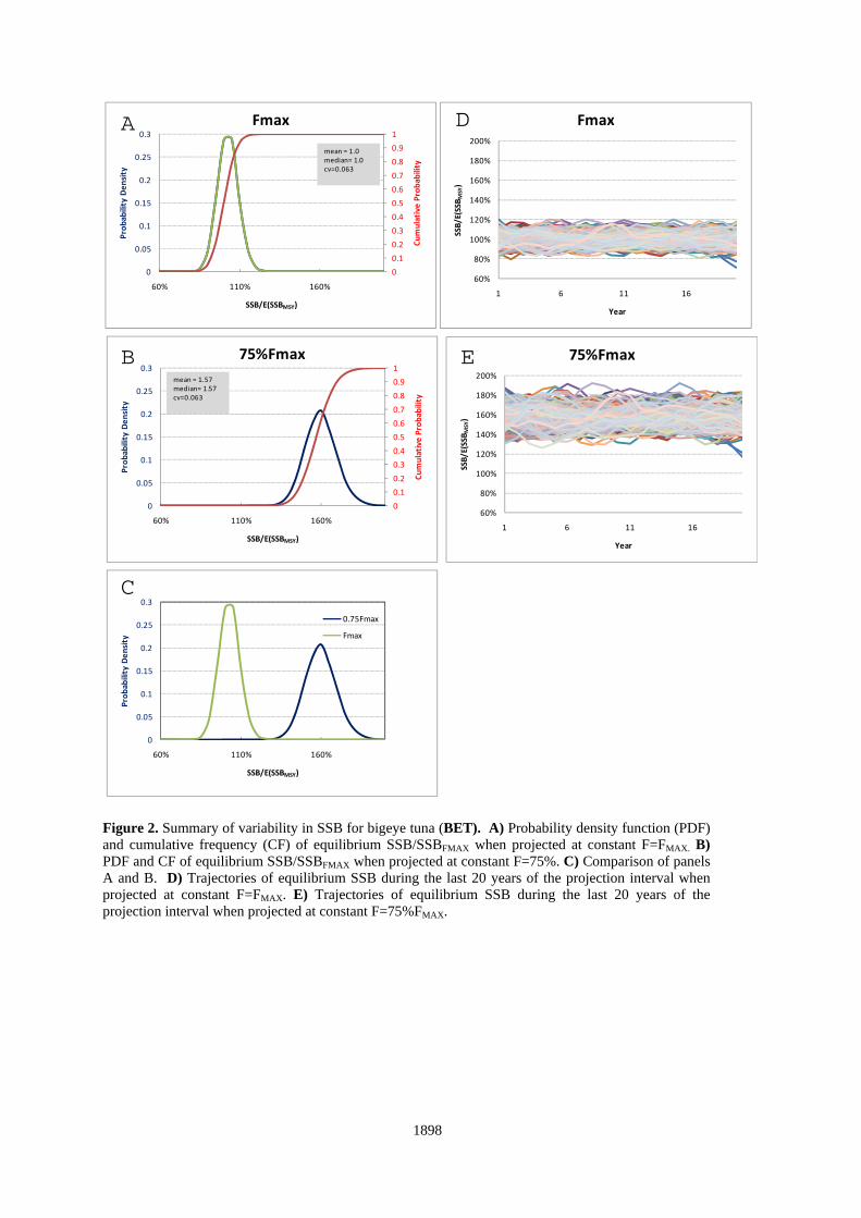
1898

Figure 2. Summary of variability in SSB for bigeye tuna (BET). A) Probability density function (PDF) and cumulative frequency (CF) of equilibrium SSB/SSBFMAX when projected at constant F=FMAX. B) PDF and CF of equilibrium SSB/SSBFMAX when projected at constant F=75%. C) Comparison of panels A and B. D) Trajectories of equilibrium SSB during the last 20 years of the projection interval when projected at constant F=FMAX. E) Trajectories of equilibrium SSB during the last 20 years of the projection interval when projected at constant F=75%FMAX.

0

0.1

0.2

0.3

0.4

0.5

0.6

0.7

0.8

0.9

1

0

0.05

0.1

0.15

0.2

0.25

0.3

60% 110% 160%

Cumulative

Probability

Probability Density

SSB/E(SSBMSY)

Fmax

mean = 1.0median= 1.0cv=0.063

60%

80%

100%

120%

140%

160%

180%

200%

1 6 11 16

SSB/E(SSB

MSY)

Year

Fmax

60%

80%

100%

120%

140%

160%

180%

200%

1 6 11 16

SSB/E(SSB

MSY)

Year

75%Fmax

0

0.1

0.2

0.3

0.4

0.5

0.6

0.7

0.8

0.9

1

0

0.05

0.1

0.15

0.2

0.25

0.3

60% 110% 160%

Cumulative

Probability

Probability Density

SSB/E(SSBMSY)

75%Fmax

mean = 1.57median= 1.57cv=0.063

0

0.05

0.1

0.15

0.2

0.25

0.3

60% 110% 160%

Probability Density

SSB/E(SSBMSY)

0.75Fmax

Fmax

A D

B

C

E

1899

Figure 3. Summary of variability in SSB for northern albacore tuna (N-ALB). A) Probability density function (PDF) and cumulative frequency (CF) of equilibrium SSB/SSBFMAX when projected at constant F=FMAX. B) PDF and CF of equilibrium SSB/SSBFMAX when projected at constant F=75%. C) Comparison of panels A and B. D) Trajectories of equilibrium SSB during the last 20 years of the projection interval when projected at constant F=FMAX. E) Trajectories of equilibrium SSB during the last 20 years of the projection interval when projected at constant F=75%FMAX.

0

0.1

0.2

0.3

0.4

0.5

0.6

0.7

0.8

0.9

1

0

0.05

0.1

0.15

0.2

0.25

60% 110% 160%

Cumulative

Probability

Probability Density

SSB/E(SSBMSY)

Fmax

mean = 1.0median= 0.986cv=0.138

60%

80%

100%

120%

140%

160%

180%

200%

220%

240%

1 6 11 16

SSB/E(SSB

MSY)

Year

Fmax

60%

80%

100%

120%

140%

160%

180%

200%

220%

240%

1 6 11 16

SSB/E(SSB

MSY)

Year

75%Fmax

0

0.1

0.2

0.3

0.4

0.5

0.6

0.7

0.8

0.9

1

0

0.05

0.1

0.15

0.2

0.25

60% 110% 160%

Cumulative

Probability

Probability Density

SSB/E(SSBMSY)

75%Fmax

mean = 1.70median= 1.68cv=0.130

0

0.05

0.1

0.15

0.2

0.25

60% 110% 160%

Probability Density

SSB/E(SSBMSY)

Fmax

0.75Fmax

A D

B

C

E

1900

Figure 4. Summary of variability in SSB for north Atlantic swordfish (N-SWO). A) Probability density function (PDF) and cumulative frequency (CF) of equilibrium SSB/SSBFMAX when projected at constant F=FMAX. B) PDF and CF of equilibrium SSB/SSBFMAX when projected at constant F=75%. C) Comparison of panels A and B. D) Trajectories of equilibrium SSB during the last 20 years of the projection interval when projected at constant F=FMAX. E) Trajectories of equilibrium SSB during the last 20 years of the projection interval when projected at constant F=75%FMAX.

0

0.1

0.2

0.3

0.4

0.5

0.6

0.7

0.8

0.9

1

0

0.05

0.1

0.15

0.2

0.25

0.3

0.35

60% 110% 160%

Cumulative

Probability

Probability Density

SSB/E(SSBMSY)

Fmax

mean = 1.0median= 0.999cv=0.052

60%

80%

100%

120%

140%

160%

180%

200%

1 6 11 16

SSB/E(SSB

MSY)

Year

Fmax

60%

80%

100%

120%

140%

160%

180%

200%

1 6 11 16

SSB/E(SSB

MSY)

Year

75%Fmax

0

0.1

0.2

0.3

0.4

0.5

0.6

0.7

0.8

0.9

1

0

0.05

0.1

0.15

0.2

0.25

0.3

0.35

60% 110% 160%

Cumulative

Probability

Probability Density

SSB/E(SSBMSY)

75%Fmax

mean = 1.53median= 1.53cv=0.046

0

0.05

0.1

0.15

0.2

0.25

0.3

0.35

60% 110% 160%

Probability Density

SSB/E(SSBMSY)

0.75Fmax

Fmax

A D

B

C

E

1901

Figure 5. Summary of variability in SSB for western bluefin tuna “2-Line/ Low Recruitment” model (W-BFT-R71+). A) Probability density function (PDF) and cumulative frequency (CF) of equilibrium SSB/SSBFMAX when projected at constant F=FMAX. B) PDF and CF of equilibrium SSB/SSBFMAX when projected at constant F=75%. C) Comparison of panels A and B. D) Trajectories of equilibrium SSB during the last 20 years of the projection interval when projected at constant F=FMAX. E) Trajectories of equilibrium SSB during the last 20 years of the projection interval when projected at constant F=75%FMAX.

0

0.1

0.2

0.3

0.4

0.5

0.6

0.7

0.8

0.9

1

0

0.05

0.1

0.15

0.2

0.25

0.3

0.35

60% 110% 160%

Cumulative

Probability

Probability Density

SSB/E(SSBMSY)

Fmax

mean = 1.0median= 0.998cv=0.062

60%

80%

100%

120%

140%

160%

180%

200%

1 6 11 16

SSB/E(SSB

MSY)

Year

Fmax

60%

80%

100%

120%

140%

160%

180%

200%

1 6 11 16

SSB/E(SSB

MSY)

Year

75%Fmax

0

0.1

0.2

0.3

0.4

0.5

0.6

0.7

0.8

0.9

1

0

0.05

0.1

0.15

0.2

0.25

0.3

0.35

60% 110% 160%

Cumulative

Probability

Probability Density

SSB/E(SSBMSY)

75%Fmax

mean = 1.37median= 1.37cv=0.055

0

0.05

0.1

0.15

0.2

0.25

0.3

0.35

60% 110% 160%

Probability Density

SSB/E(SSBMSY)

Fmax

0.75Fmax

A D

B

C

E

1902

Figure 6. Summary of variability in SSB for western bluefin tuna “Beverton&Holt/ High Recruitment” model (W-BFT-R76+). A) Probability density function (PDF) and cumulative frequency (CF) of equilibrium SSB/SSBFMAX when projected at constant F=FMAX. B) PDF and CF of equilibrium SSB/SSBFMAX when projected at constant F=75%. C) Comparison of panels A and B. D) Trajectories of equilibrium SSB during the last 20 years of the projection interval when projected at constant F=FMAX. E) Trajectories of equilibrium SSB during the last 20 years of the projection interval when projected at constant F=75%FMAX.

0

0.1

0.2

0.3

0.4

0.5

0.6

0.7

0.8

0.9

1

0

0.05

0.1

0.15

0.2

0.25

60% 110% 160%

Cumulative

Probability

Probability Density

SSB/E(SSBMSY)

Fmax

mean = 1.0median= 0.979cv=0.173

60%

80%

100%

120%

140%

160%

180%

200%

1 6 11 16

SSB/E(SSB

MSY)

Year

Fmax

60%

80%

100%

120%

140%

160%

180%

200%

1 6 11 16

SSB/E(SSB

MSY)

Year

75%Fmax

0

0.1

0.2

0.3

0.4

0.5

0.6

0.7

0.8

0.9

1

0

0.05

0.1

0.15

0.2

0.25

60% 110% 160%

Cumulative

Probability

Probability Density

SSB/E(SSBMSY)

75%Fmax

mean = 1.38median= 1.36cv=0.153

0

0.05

0.1

0.15

0.2

0.25

60% 110% 160%

Probability Density

SSB/E(SSBMSY)

Fmax

0.75Fmax

A D

B

C

E

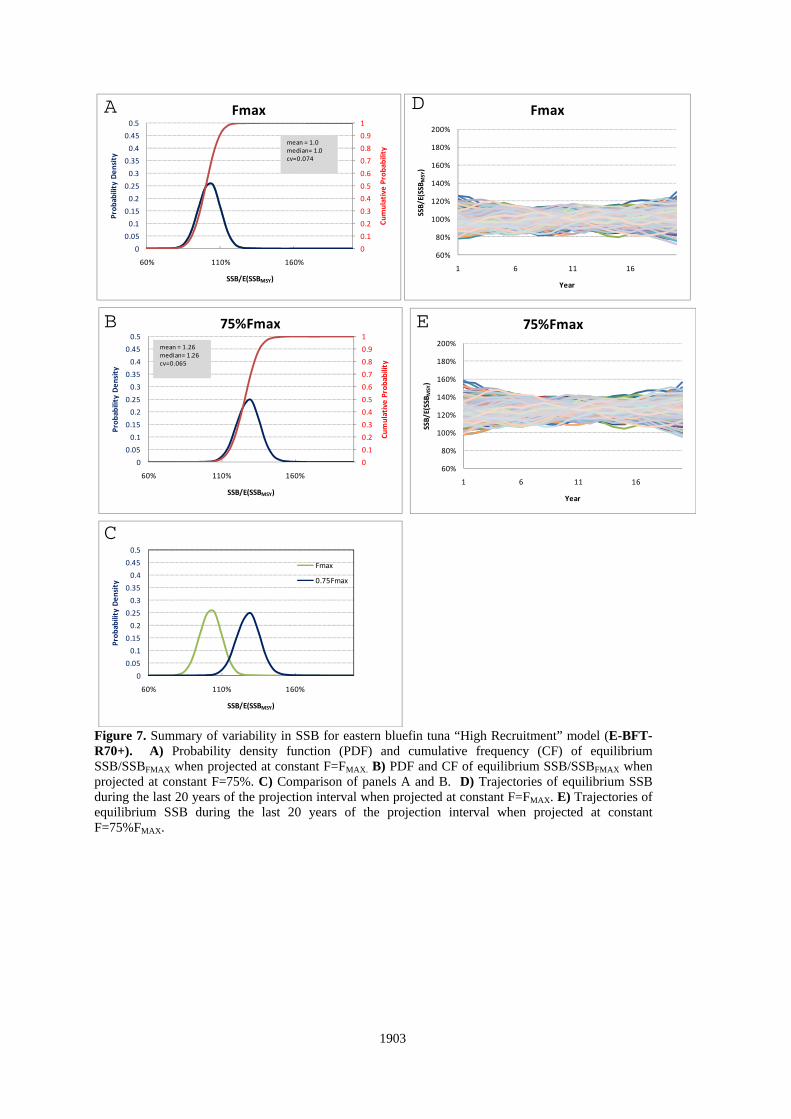
1903

Figure 7. Summary of variability in SSB for eastern bluefin tuna “High Recruitment” model (E-BFT-R70+). A) Probability density function (PDF) and cumulative frequency (CF) of equilibrium SSB/SSBFMAX when projected at constant F=FMAX. B) PDF and CF of equilibrium SSB/SSBFMAX when projected at constant F=75%. C) Comparison of panels A and B. D) Trajectories of equilibrium SSB during the last 20 years of the projection interval when projected at constant F=FMAX. E) Trajectories of equilibrium SSB during the last 20 years of the projection interval when projected at constant F=75%FMAX.

0

0.1

0.2

0.3

0.4

0.5

0.6

0.7

0.8

0.9

1

0

0.05

0.1

0.15

0.2

0.25

0.3

0.35

0.4

0.45

0.5

60% 110% 160%

Cumulative

Probability

Probability Density

SSB/E(SSBMSY)

Fmax


60%

80%

100%

120%

140%

160%

180%

200%

1 6 11 16

SSB/E(SSB

MSY)

Year

Fmax

60%

80%

100%

120%

140%

160%

180%

200%

1 6 11 16

SSB/E(SSB

MSY)

Year

75%Fmax

0

0.1

0.2

0.3

0.4

0.5

0.6

0.7

0.8

0.9

1

0

0.05

0.1

0.15

0.2

0.25

0.3

0.35

0.4

0.45

0.5

60% 110% 160%

Cumulative

Probability

Probability Density

SSB/E(SSBMSY)

75%Fmax

mean = 1.26median= 1.26cv=0.065

0

0.05

0.1

0.15

0.2

0.25

0.3

0.35

0.4

0.45

0.5

60% 110% 160%

Probability Density

SSB/E(SSBMSY)

Fmax

0.75Fmax

A D

B

C

E

1904

Figure 8. Summary of variability in SSB for eastern bluefin tuna “Low Recruitment” model (E-BFT-R90+). A) Probability density function (PDF) and cumulative frequency (CF) of equilibrium SSB/SSBFMAX when projected at constant F=FMAX. B) PDF and CF of equilibrium SSB/SSBFMAX when projected at constant F=75%. C) Comparison of panels A and B. D) Trajectories of equilibrium SSB during the last 20 years of the projection interval when projected at constant F=FMAX. E) Trajectories of equilibrium SSB during the last 20 years of the projection interval when projected at constant F=75%FMAX.

0

0.1

0.2

0.3

0.4

0.5

0.6

0.7

0.8

0.9

1

0

0.05

0.1

0.15

0.2

0.25

0.3

0.35

0.4

0.45

0.5

60% 110% 160%

Cumulative

Probability

Probability Density

SSB/E(SSBMSY)

Fmax


60%

80%

100%

120%

140%

160%

180%

200%

1 6 11 16

SSB/E(SSB

MSY)

Year

Fmax

60%

80%

100%

120%

140%

160%

180%

200%

1 6 11 16

SSB/E(SSB

MSY)

Year

75%Fmax

0

0.1

0.2

0.3

0.4

0.5

0.6

0.7

0.8

0.9

1

0

0.05

0.1

0.15

0.2

0.25

0.3

0.35

0.4

0.45

0.5

60% 110% 160%

Cumulative

Probability

Probability Density

SSB/E(SSBMSY)

75%Fmax

mean = 1.26median= 1.26cv=0.031

0

0.05

0.1

0.15

0.2

0.25

0.3

0.35

0.4

0.45

0.5

60% 110% 160%

Probability Density

SSB/E(SSBMSY)

Fmax

0.75Fmax

A D

B

C

E

1905

Figure 9. Summary of variability in fishable biomass (FB) for yellowfin tuna (YFT). A) Probability density function (PDF) and cumulative frequency (CF) of equilibrium FB/FBFMAX when projected at constant F=FMAX. B) PDF and CF of equilibrium FB/FBFMAX when projected at constant F=75%. C) Comparison of panels A and B. D) Trajectories of equilibrium FB during the last 20 years of the projection interval when projected at constant F=FMAX. E) Trajectories of equilibrium FB during the last 20 years of the projection interval when projected at constant F=75%FMAX.

0

0.1

0.2

0.3

0.4

0.5

0.6

0.7

0.8

0.9

1

0

0.05

0.1

0.15

0.2

0.25

0.3

0.35

60% 80% 100% 120% 140%

Cumulative

Probability

Probability Density

FB/E(FBMSY)

Fmax

mean = 1.0median= 0.998cv=0.067

60%

80%

100%

120%

140%

160%

180%

200%

1 6 11 16

FB/E(FBMSY)

Year

Fmax

60%

80%

100%

120%

140%

160%

180%

200%

1 6 11 16

FB/E(FBMSY)

Year

75%Fmax

0

0.1

0.2

0.3

0.4

0.5

0.6

0.7

0.8

0.9

1

0

0.05

0.1

0.15

0.2

0.25

60% 110% 160%

Cumulative

Probability

Probability Density

FB/E(FBMSY)

75%Fmax

mean = 1.30median= 1.30cv=0.068

0

0.05

0.1

0.15

0.2

0.25

0.3

0.35

60% 110% 160%

Probability Density

FB/E(FBMSY)

Fmax

0.75Fmax

A D

B

C

E

1906

Figure 10. Summary of variability in fishable biomass (FB) for bigeye tuna (BET). A) Probability density function (PDF) and cumulative frequency (CF) of equilibrium FB/FBFMAX when projected at constant F=FMAX. B) PDF and CF of equilibrium FB/FBFMAX when projected at constant F=75%. C) Comparison of panels A and B. D) Trajectories of equilibrium FB during the last 20 years of the projection interval when projected at constant F=FMAX. E) Trajectories of equilibrium FB during the last 20 years of the projection interval when projected at constant F=75%FMAX.

0

0.1

0.2

0.3

0.4

0.5

0.6

0.7

0.8

0.9

1

0

0.05

0.1

0.15

0.2

0.25

0.3

0.35

60% 80% 100% 120% 140%

Cumulative

Probability

Probability Density

FB/E(FBMSY)

Fmax


60%

80%

100%

120%

140%

160%

180%

200%

1 6 11 16

FB/E(FBMSY)

Year

Fmax

60%

80%

100%

120%

140%

160%

180%

200%

1 6 11 16

FB/E(FBMSY)

Year

75%Fmax

0

0.1

0.2

0.3

0.4

0.5

0.6

0.7

0.8

0.9

1

0

0.05

0.1

0.15

0.2

0.25

0.3

0.35

60% 110% 160%

Cumulative

Probability

Probability Density

FB/E(FBMSY)

75%Fmax

mean = 1.36median= 1.36cv=0.051

0

0.05

0.1

0.15

0.2

0.25

0.3

0.35

60% 110% 160%

Probability Density

FB/E(FBMSY)

Fmax

0.75Fmax

A D

B

C

E

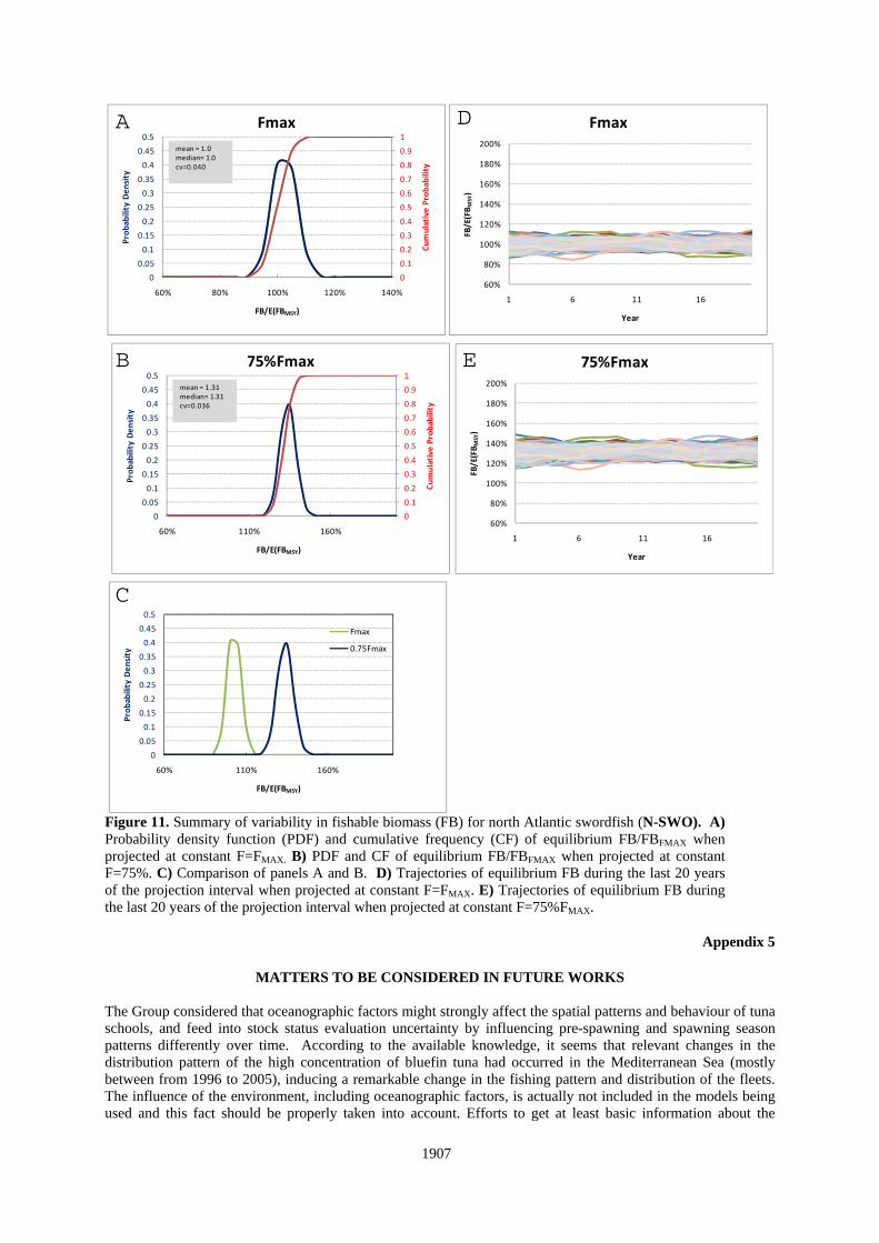
1907

Figure 11. Summary of variability in fishable biomass (FB) for north Atlantic swordfish (N-SWO). A) Probability density function (PDF) and cumulative frequency (CF) of equilibrium FB/FBFMAX when projected at constant F=FMAX. B) PDF and CF of equilibrium FB/FBFMAX when projected at constant F=75%. C) Comparison of panels A and B. D) Trajectories of equilibrium FB during the last 20 years of the projection interval when projected at constant F=FMAX. E) Trajectories of equilibrium FB during the last 20 years of the projection interval when projected at constant F=75%FMAX.

Appendix 5

MATTERS TO BE CONSIDERED IN FUTURE WORKS

The Group considered that oceanographic factors might strongly affect the spatial patterns and behaviour of tuna schools, and feed into stock status evaluation uncertainty by influencing pre-spawning and spawning season patterns differently over time. According to the available knowledge, it seems that relevant changes in the distribution pattern of the high concentration of bluefin tuna had occurred in the Mediterranean Sea (mostly between from 1996 to 2005), inducing a remarkable change in the fishing pattern and distribution of the fleets. The influence of the environment, including oceanographic factors, is actually not included in the models being used and this fact should be properly taken into account. Efforts to get at least basic information about the

0

0.1

0.2

0.3

0.4

0.5

0.6

0.7

0.8

0.9

1

0

0.05

0.1

0.15

0.2

0.25

0.3

0.35

0.4

0.45

0.5

60% 80% 100% 120% 140%

Cumulative

Probability

Probability Density

FB/E(FBMSY)

Fmax


60%

80%

100%

120%

140%

160%

180%

200%

1 6 11 16

FB/E(FBMSY)

Year

Fmax

60%

80%

100%

120%

140%

160%

180%

200%

1 6 11 16

FB/E(FBMSY)

Year

75%Fmax

0

0.1

0.2

0.3

0.4

0.5

0.6

0.7

0.8

0.9

1

0

0.05

0.1

0.15

0.2

0.25

0.3

0.35

0.4

0.45

0.5

60% 110% 160%

Cumulative

Probability

Probability Density

FB/E(FBMSY)

75%Fmax

mean = 1.31median= 1.31cv=0.036

0

0.05

0.1

0.15

0.2

0.25

0.3

0.35

0.4

0.45

0.5

60% 110% 160%

Probability Density

FB/E(FBMSY)

Fmax

0.75Fmax

A D

B

C

E

1908

environmentally related distribution variables may help to better quantify uncertainty in stock status evaluations for some species. The Group also considered that the use of the available information on the fleet spatial distribution and concentrations (VMS aggregated data by gear and time strata) is expected to add significant understanding of fishing strategies coincident with environmental changes and fish movements. Combining VMS with remotely sensed environmental information would also contribute to an improved understanding of fish and fishery dynamics. Methods to fully utilize VMS and auxiliary data for support of stock status evaluations should be a focus for future application in providing advice to the Commission on stock status and availability.