Embed Size (px)
Citation preview
October 1988 Denver Off ice
3epartment of the Interior of Reclamation
7-2090 (4-81) Bureau of Reclamation TECHNICAL REPORT STANDARD TITLE PAGE
Cone Penetration Testing
-
- 1
- 1
- 1
for Evaluating the ~ i ~ u e f i c t i o n Potential of Sands
I
R M l N G O R G A N I Z A T I O N C O D E
r ' I D- 1 542 r Lm-< -, . ' E ' j . ; -
7. AUTHOR^) 8 P E R F O R M I N G O R G A N I Z A T I O N R E P O R T NO.
Robert R. Carter REC-ERC-87-9
Same I
--
9 . P E R F O R M l k
Bureau of Denver 0' Denver, CO 80225
2 . SPONSORING A G E N C Y N A M E A N D ADDRESS
14. SPONSORING A G E N C Y C O D E
DlBR 5 . S U P P L E M E N T A R Y N O T E S
10. WORK U N I T NO.
1 1 . C O N T R A C T OR G R A N T NO.
13. T Y P E O F R E P O R T A N D P E R I O D C O V E R E D
Microfiche and hard copy available from the Denver office, Denver, Colorado
Editor:RC(c)/SA
6 . A B S T R A C T
The purpose of this report is to present the state of the art for the cone penetration test as an in situ tool for determining the dynamic response of sands during earthquake loading. Although a vast amount of literature has been published over the past 20 years on cone penetration testing, on the dynamic response of sands, and on their correlation, little agree- ment has been reached in any of these areas. Lack of a common ground has produced both progress and confusion.
This report presents not only the current methods of relating cone penetration test data to the dynamic response of sands, but also the current concepts and theories related to each of them. Based on the information presented in this review, the author draws conclusions on the appropriateness and value of established cone penetration resistance - earthquake loading response of sand relationships and on areas in which further research is needed to produce a complete and consistent method for producing such a relationship.
7. K E Y WORDS A N D D O C U M E N T A N A L Y S I S
3. D E S C R I P T O R S - - cone penetration test/ soil dynamics/ sands/ soil models/ liquefaction/ compressibility
c . C O S A T I F i e l d / G r o u p 08M COWRR: 0813 SR IM:
2 1 . N O . O F P A G E
60 2 2 . P R I C E
18. D I S T R I B U T I O N S T A T E M E N T
A v a i l a b l e from t h e N o t i o n a l T e c h n i c a l In fo rmat ion S e r v i c e , Opera t ions D i v i s i o n . 5285 Por t R o y a l Road. Spr ing f ie :d . V i r g i n i a 22161.
(Microfiche and hard copy available from NTIS)
1 9 . S E C U R I T Y C L A S S ( T H I S R E P O R T )
U N C L A S S I F I E D 2 0 . S E C U R I T Y CLASS
( T H I S PAGE)
U N C L A S S I F I E D
CONE PENETRATION TESTING FOR EVALUATING THE LIQUEFACTION POTENTIAL OF SANDS
bv
Robert R. Carter
May 1988
Geotechnical Services Branch Research and Laboratory. Services Division., Denver. Colorado
UNITED STATES DEPARTMENT OF THE INTERIOR * j BUREAU OF RECLAMATION
ACKNOWLEDGMENTS
This report was submitted to the Department of Civil, Environmental, and Architectural Engineering of theGraduate School of the University of Colorado in 1987, in partial fulfillment of the requirements for thedegree of Master of Science.
As the Nation's principal conservation agency, the Department of theInterior has responsibility for most of our nationally owned publiclands and natural resources. This includes fostering the wisest use ofour land and water resources, protecting our fish and wildlife, preserv-ing the environmental and cultural values of our national parks andhistorical places, and providing for the enjoyment of life through out-door recreation. The Department assesses our energy and mineralresources and works to assure that their development is in the bestinterests of all our people. The Department also has a major respon-sibility for American Indian reservation communities and for peoplewho live in Island Territories under U.S. Administration.
The information contained in th is report regarding commercial prod-ucts or firms may not be used for advertising or promotional purposesand is not to be construed as an endorsement of any product or firmby the Bureau of Reclamation.
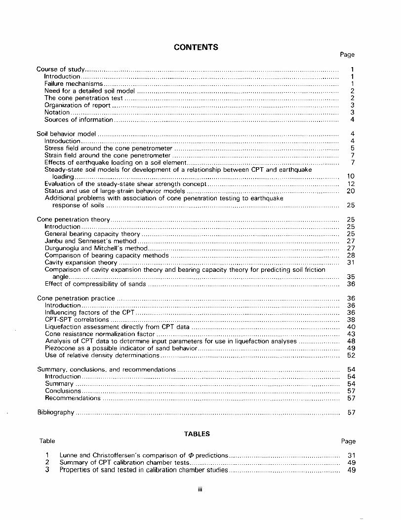
CONTENTS
Course of study ..Introduction ..,.......Failure mechanisms..................................................................................................................Need for a detailed soil model , , """""'" ..,.......
The cone penetration test ,.......Organization of report..............................................................................................................Notation ..,.......Sources of information.............................................................................................................
Soil behavior model ,..............................Introduction ,.......Stress field around the cone penetrometer................................................................................Strain field around the cone penetrometer.................................................................................Effects of earthquake loading on a soil element..........................................................................Steady-state soil models for development of a relationship between CPT and earthquake
loading """'"
Evaluation of the steady-state shear strength concept................................................................Status and use of large-strain behavior models ,.......Additional problems with association of cone penetration testing to earthquake
response of soils.................................................................................................................
Cone penetration theory...............................................................................................................Introduction ..,.......General bearing capacity theory................................................................................................Janbu and Senneset's method..................................................................................................Durgunoglu and Mitchell's method.............................................................................................Comparison of bearing capacity methods..................................................................................Cavity expansion theory...........................................................................................................Comparison of cavity expansion theory and bearing capacity theory for predicting soil friction
angle , ,.......
Effect of compressibility of sands.............................................................................................
Cone penetration practice............................................................................................................Introduction ..,.......Influencing factors of the CPT...................................................................................................CPT-SPT correlations...............................................................................................................Liquefaction assessment directly from CPT data ,.......Cone resistance normalization factor.........................................................................................Analysis of CPT data to determine input parameters for use in liquefaction analyses....................Piezocone as a possible indicator of sand behavior.....................................................................Use of relative density determinations.......................................................................................
Summary, conclusions, and recommendations...............................................................................Introduction ..,.......Summary . ..,.. ..
""". .
"""". , .. . . . , . . ,.. .....
Conclusions.. . , , . . . ,.. .....Recommendations ....
Bibliography ,.......
TABLESTable
123
Lunne and Christoffersen's comparison of cPpredictions......................................................Summary of CPT calibration chamber tests """ ...,........
Properties of sand tested in calibration chamber studies......................................................
III
Page
11122334
44577
101220
25
25252527272831
3536
363636384043484952
5454545757
57
Page
314949
Figure
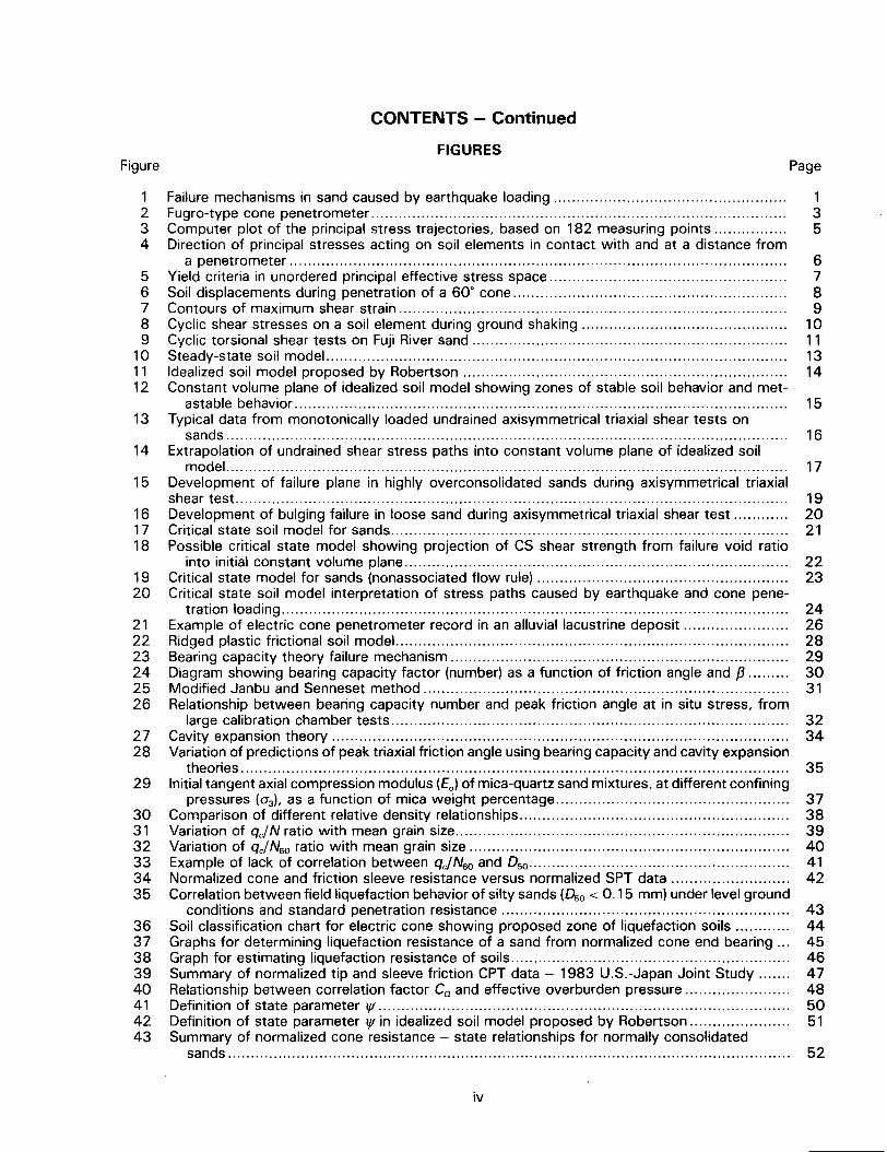
CONTENTS - Continued
FIGURES
1234
Failure mechanisms in sand caused by earthquake loading...................................................Fugro-type cone penetrometer...........................................................................................Computer plot of the principal stress trajectories, based on 182 measuring points................Direction of principal stresses acting on soil elements in contact with and at a distance from
a penetrometer.............................................................................................................Yield criteria in unordered principal effective stress space....................................................Soil displacements during penetration of a 60. cone............................................................Contours of maximum shear strain.....................................................................................Cyclic shear stresses on a soil element during ground shaking.............................................Cyclic torsional shear tests on Fuji River sand.....................................................................Steady-state soil model.....................................................................................................Idealized soil model proposed by Robertson.......................................................................Constant volume plane of idealized soil model showing zones of stable soil behavior and met-
astable behavior............................................................................................................Typical data from monotonically loaded undrained axisymmetrical triaxial shear tests on
sands ..Extrapolation of undrained shear stress paths into constant volume plane of idealized soil
model """""""""""""""""""""""""""....................
Development of failure plane in highly overconsolidated sands during axisymmetrical triaxialshear test.........................................................................................................................Development of bulging failure in loose sand during axisymmetrical triaxial shear test............Critical state soil model for sands.......................................................................................Possible critical state model showing projection of CS shear strength from failure void ratio
into initial constant volume plane....................................................................................Critical state model for sands (nonassociated flow rule) .......................................................Critical state soil model interpretation of stress paths caused by earthquake and cone pene-
tration loading...............................................................................................................Example of electric cone penetrometer record in an alluvial lacustrine deposit.......................Ridged plastic frictional soil model......................................................................................Bearing capacity theory failure mechanism..........................................................................Diagram showing bearing capacity factor (number) as a function of friction angle and {3.........Modified Janbu and Senneset method...
"""'"... ""'" ......
Relationship between bearing capacity number and peak friction angle at in situ stress, fromlarge calibration chamber tests.......................................................................................
Cavity expansion theory....................................................................................................Variation of predictions of peak triaxial friction angle using bearing capacity and cavity expansion
theories... . . . . . . .. . .. . . . . . . . . ."""
.. . . . . . . . . .. . ... . . . ... . . . . ... . . . ... . .'"
. ... . . . ... .Initial tangent axial compression modulus (Eo) of mica-quartz sand mixtures, at different confining
pressures (()3), as a function of mica weight percentage...................................................Comparison of different relative density relationships "'" "'" ......
Variation of qc/ N ratio with mean grain size.........................................................................Variation of qc/ Nso ratio with mean grain size......................................................................Example of lack of correlation between qc/ Nso and D50"'"''''''''''''''''''''''''''''''''''''''''''''''''''''Normalized cone and friction sleeve resistance versus normalized SPT data..........................Correlation between field liquefaction behavior of silty sands (D50 < 0.15 mm) under level ground
conditions and standard penetration resistance """ ... ... ...Soil classification chart for electric cone showing proposed zone of liquefaction soils............Graphs for determining liquefaction resistance of a sand from normalized cone end bearing...Graph for estimating liquefaction resistance of soils.............................................................Summary of normalized tip and sleeve friction CPT data - 1983 U.S.-Japan Joint Study.......Relationship between correlation factor Co and effective overburden pressure.......................Definition of state parameter 'If """'" """ "'" ......
Definition of state parameter 'If in idealized soil model proposed by Robertson......................Summary of normalized cone resistance - state relationships for normally consolidated
sands ..
56789
101112
13
14
15
161718
1920
212223242526
2728
29
303132333435
3637383940414243
iv
Page
135
6789
10111314
15
16
17
192021
2223
242628293031
3234
35
373839404142
4344454647485051
52
Figures
CONTENTS - Continued
444546
4748
Location of filter elements for measurement of pore pressure..............................................Conceptual pore pressure distribution in saturated soil during cone penetration.....................Piezocone data showing lack of response of pore pressure measurements to changing soil
types. .. ...... .. ...... ... ..."""
.. .... ..... ................. ... .. ............ ......Conceptual plots of pore pressure decay patterns measured behind the cone........................Examples of change in pore pressure measurements due to densification of sands and silts...
v
Page
5353
545556

COURSE OF STUDY
Introduction
Before the Niigata and Alaskan earthquakes of 1964,most geotechnical engineers had expressed littleconcern about the dynamic behavior of saturatedsand layers. Regardless of their density, sands weregenerally considered quite incompressible and stablefor foundation and construction uses. The only dis-advantages for the universal use of sands consideredwere the consequences of their high permeabilities:excessive seepage losses, high exit gradients (whichcould reach critical or flotation gradient levels), andthe possibility of adjoining fine-grained soils pipinginto the voids of the sand. Each of these problemswas concerned with the steady-state flow of waterthrough sand. Damage to many structures foundedon saturated sand beds and other physical signs ofloss of strength in sand layers during the two 1964earthquakes resulted in the formation of a new areaof geotechnical engineering. And new term, "lique-faction," was coined to describe the more visibleoutcomes of earthquake-related failures.
Failure Mechanisms
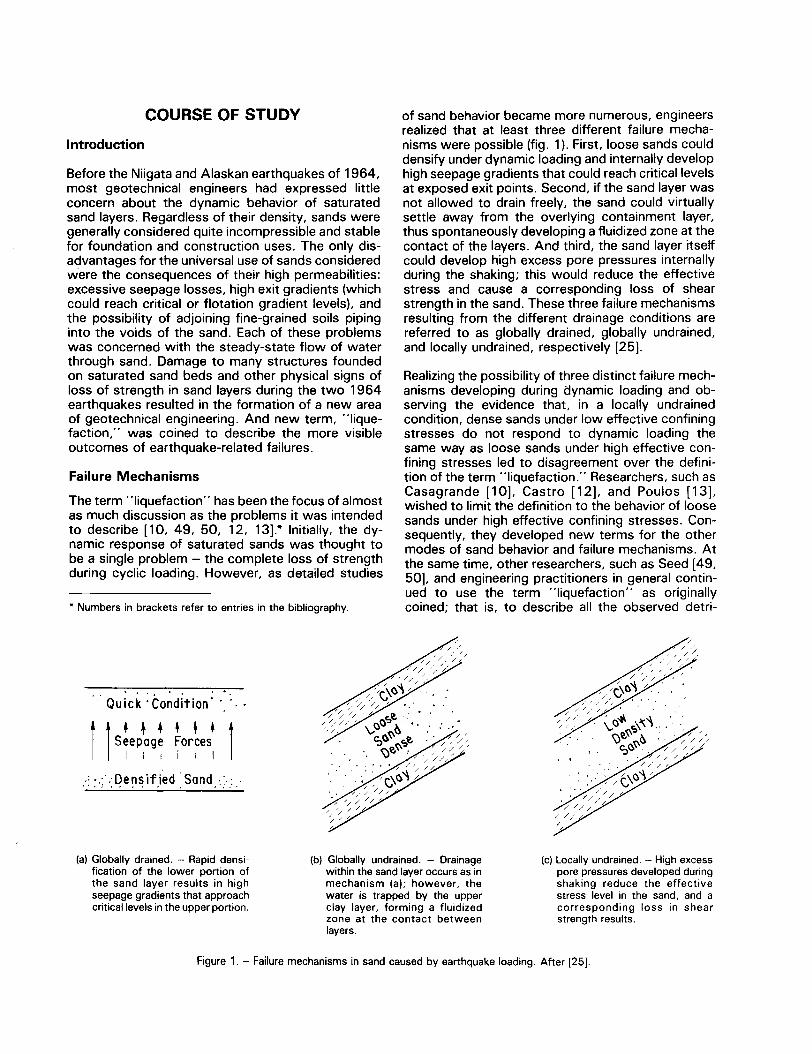
The term "liquefaction" has been the focus of almostas much discussion as the problems it was intendedto describe [10, 49, 50, 12, 13].* Initially, the dy-namic response of saturated sands was thought tobe a single problem - the complete loss of strengthduring cyclic loading. However, as detailed studies
. Numbers in brackets refer to entries in the bibliography.
of sand behavior became more numerous, engineersrealized that at least three different failure mecha-nisms were possible (fig. 1). First, loose sands coulddensify under dynamic loading and internally develophigh seepage gradients that could reach critical levelsat exposed exit points. Second, if the sand layer wasnot allowed to drain freely, the sand could virtuallysettle away from the overlying containment layer,thus spontaneously developing a fluidized zone at thecontact of the layers. And third, the sand layer itselfcould develop high excess pore pressures internallyduring the shaking; this would reduce the effectivestress and cause a corresponding loss of shearstrength in the sand. These three failure mechanismsresulting from the different drainage conditions arereferred to as globally drained, globally undrained,and locally undrained, respectively [25].
Realizing the possibility of three distinct failure mech-anisms developing during dynamic loading and ob-serving the evidence that, in a locally undrainedcondition, dense sands under low effective confiningstresses do not respond to dynamic loading thesame way as loose sands under high effective con-fining stresses led to disagreement over the defini-tion of the term "liquefaction." Researchers, such asCasagrande [1°], Castro [12], and Poulos [13],wished to limit the definition to the behavior of loosesands under high effective confining stresses. Con-sequently, they developed new terms for the othermodes of sand behavior and failure mechanisms. Atthe same time, other researchers, such as Seed [49,50], and engineering practitioners in general contin-ued to use the term "liquefaction" as originallycoined; that is, to describe all the observed detri-
. ,.
Quick 'Condition",'..
11s~ep+ag~ ~or~es. t
I I i I I I I
:: :-;'.:qe ~~if,ied :Sand, ::.-.: ..
(a) Globally drained. - Rapid densi-
fication of the lower portion ofthe sand layer results in highseepage gradients that approachcritical levels in the upper portion.
(b) Globally undrained. - Drainage
within the sand layer occurs as inmechanism (a); however, thewater is trapped by the upperclay layer, forming a fluidizedzone at the contact betweenlayers.
(c) Locally undrained. - High excesspore pressures developed duringshaking reduce the effectivestress level in the sand, and acorresponding loss in shearstrength results.
Figure 1. - Failure mechanisms in sand caused by earthquake loading. After [25].
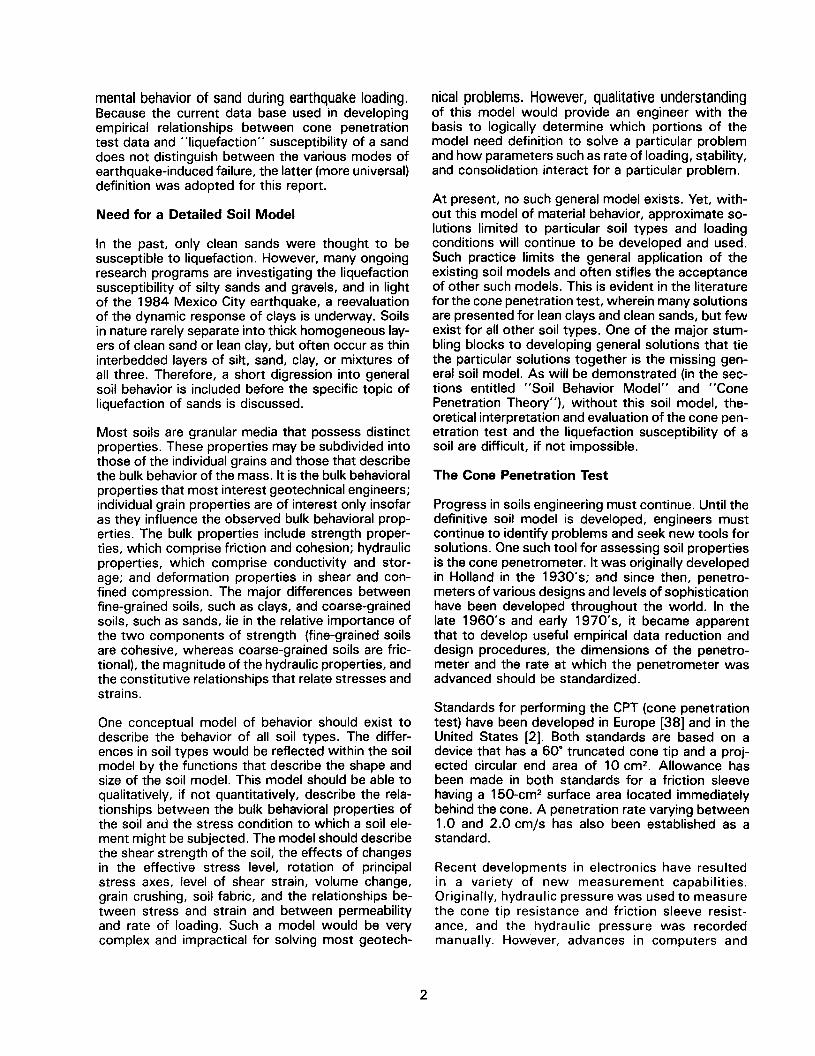
mental behavior of sand during earthquake loading.Because the current data base used in developingempirical relationships between cone penetrationtest data and "liquefaction" susceptibility of a sanddoes not distinguish between the various modes ofearthquake-induced failure, the latter (more universal)definition was adopted for this report.
Need for a Detailed Soil Model
In the past, only clean sands were thought to besusceptible to liquefaction. However, many ongoingresearch programs are investigating the liquefactionsusceptibility of silty sands and gravels, and in lightof the 1984 Mexico City earthquake, a reevaluationof the dynamic response of clays is underway. Soilsin nature rarely separate into thick homogeneous lay-ers of clean sand or lean clay, but often occur as thininterbedded layers of silt, sand, clay, or mixtures ofall three. Therefore, a short digression into generalsoil behavior is included before the specific topic ofliquefaction of sands is discussed.
Most soils are granular media that possess distinctproperties. These properties may be subdivided intothose of the individual grains and those that describethe bulk behavior of the mass. It is the bulk behavioralproperties that most interest geotechnical engineers;individual grain properties are of interest only insofaras they influence the observed bulk behavioral prop-erties. The bulk properties include strength proper-ties, which comprise friction and cohesion; hydraulicproperties, which comprise conductivity and stor-age; and deformation properties in shear and con-fined compression. The major differences betweenfine-grained soils, such as clays, and coarse-grainedsoils, such as sands, lie in the relative importance ofthe two components of strength (fine-grained soilsare cohesive, whereas coarse-grained soils are fric-tional). the magnitude of the hydraulic properties, andthe constitutive relationships that relate stresses andstrains.
One conceptual model of behavior should exist todescribe the behavior of all soil types. The differ-ences in soil types would be reflected within the soilmodel by the functions that describe the shape andsize of the soil model. This model should be able toqualitatively, if not quantitatively, describe the rela-tionships betwden the bulk behavioral properties ofthe soil and the stress condition to which a soil ele-ment might be subjected. The model should describethe shear strength of the soil, the effects of changesin the effective stress level, rotation of principalstress axes, level of shear strain, volume change,grain crushing, soil fabric, and the relationships be-tween stress and strain and between permeabilityand rate of loading. Such a model would be verycomplex and impractical for solving most geotech-
nical problems. However, qualitative understandingof this model would provide an engineer with thebasis to logically determine which portions of themodel need definition to solve a particular problemand how parameters such as rate of loading, stability,and consolidation interact for a particular problem.
At present, no such general model exists. Yet, with-out this model of material behavior, approximate so-lutions limited to particular soil types and loadingconditions will continue to be developed and used.Such practice limits the general application of theexisting soil models and often stifles the acceptanceof other such models. This is evident in the literaturefor the cone penetration test, wherein many solutionsare presented for lean clays and clean sands, but fewexist for all other soil types. One of the major stum-bling blocks to developing general solutions that tiethe particular solutions together is the missing gen-eral soil model. As will be demonstrated (in the sec-tions entitled "Soil Behavior Model" and "ConePenetration Theory"), without this soil model, the-oretical interpretation and evaluation of the cone pen-etration test and the liquefaction susceptibility of asoil are difficult, if not impossible.
The Cone Penetration Test
Progress in soils engineering must continue. Until thedefinitive soil model is developed, engineers mustcontinue to identify problems and seek new tools forsolutions. One such tool for assessing soil propertiesis the cone penetrometer. It was originally developedin Holland in the 1930' s; and since then, penetro-meters of various designs and levels of sophisticationhave been developed throughout the world. In thelate 1960's and early 1970's, it became apparentthat to develop useful empirical data reduction anddesign procedures, the dimensions of the penetro-meter and the rate at which the penetrometer wasadvanced should be standardized.
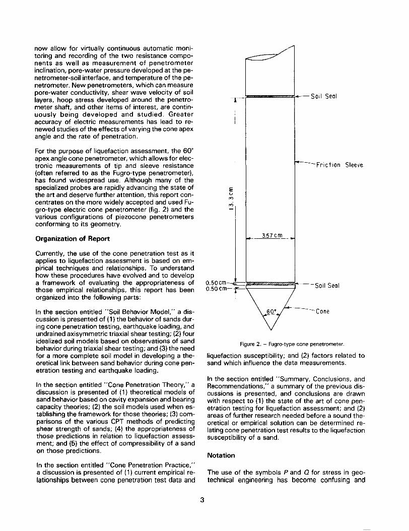
Standards for performing the CPT (cone penetrationtest) have been developed in Europe [38] and in theUnited States [2]. Both standards are based on adevice that has a 60. truncated cone tip and a proj-ected circular end area of 10 cm2. Allowance hasbeen made in both standards for a friction sleevehaving a 150-cm2 surface area located immediatelybehind the cone. A penetration rate varying between1.0 and 2.0 cm/s has also been established as astandard.
Recent developments in electronics have resultedin a variety of new measurement capabilities.Originally, hydraulic pressure was used to measurethe cone tip resistance and friction sleeve resist-ance, and the hydraulic pressure was recordedmanually. However, advances in computers and
2
now allow for virtually continuous automatic moni-toring and recording of the two resistance compo-nents as well as measurement of penetrometerinclination, pore-water pressure developed at the pe-netrometer-soil interface, and temperature of the pe-netrometer. New penetrometers, which can measurepore-water conductivity, shear wave velocity of soillayers, hoop stress developed around the penetro-meter shaft, and other items of interest, are contin-uously being developed and studied. Greateraccuracy of electric measurements has lead to re-newed studies of the effects of varying the cone apexangle and the rate of penetration.
For the purpose of liquefaction assessment, the 60.apex angle cone penetrometer, which allows for elec-tronic measurements of tip and sleeve resistance(often referred to as the Fugro-type penetrometer),has found widespread use. Although many of thespecialized probes are rapidly advancing the state ofthe art and deserve further attention, this report con-centrates on the more widely accepted and used Fu-gro-type electric cone penetrometer (fig. 2) and thevarious configurations of piezocone penetrometersconforming to its geometry.
Organization of Report
Currently, the use of the cone penetration test as itapplies to liquefaction assessment is based on em-pirical techniques and relationships. To understandhow these procedures have evolved and to developa framework of evaluating the appropriateness ofthose empirical relationships, this report has beenorganized into the following parts:
In the section entitled "Soil Behavior Model," a dis-cussion is presented of (1) the behavior of sands dur-ing cone penetration testing, earthquake loading, andundrained axisymmetric triaxial shear testing; (2) fouridealized soil models based on observations of sandbehavior during triaxial shear testing; and (3) the needfor a more complete soil model in developing a the-oreticallink between sand behavior during cone pen-etration testing and earthquake loading.
In the section entitled "Cone Penetration Theory," adiscussion is presented of (1) theoretical models ofsand behavior based on cavity expansion and bearingcapacity theories; (2) the soil models used when es-tablishing the framework for those theories; (3) com-parisons of the various CPT methods of predictingshear strength of sands; (4) the appropriateness ofthose predictions in relation to liquefaction assess-ment; and (5) the effect of compressibility of a sandon those predictions.
In the section entitled "Cone Penetration Practice,"a discussion is presented of (1) current empirical re-lationships between cone penetration test data and
5011 Seal
Fri etlan Sleeve
Eur<'>rri
3.57 em
0.50em---0.50 emT
-5011 Seal
-Cone
Figure 2. - Fugro-type cone penetrometer.
liquefaction susceptibility; and (2) factors related tosand which influence the data measurements.
In the section entitled "Summary, Conclusions, andRecommendations," a summary of the previous dis-cussions is presented, and conclusions are drawnwith respect to (1) the state of the art of cone pen-etration testing for liquefaction assessment; and (2)areas of further research needed before a sound the-oretical or empirical solution can be determined re-lating cone penetration test results to the liquefactionsusceptibility of a sand.
Notation
The use of the symbols P and Q for stress in geo-technical engineering has become confusing and
3
requires definition. In the United States, P' and Q aredefined by:
P' = 1/2 (a', + 0'3)
and
Q=1/2(o',-o'3)where:
0', = major principal effective stress, anda' 3 = minor principal effective stress.
However, in the United Kingdom and many otherparts of the world:
P' = 1/3 (a', + 0'2 + 0'3) (3)
and
Q = (a', - d 3)where:
0'2 = intermediate principal effectivestress.
To avoid confusion over the terms P' and Q, thisreport adopts the following notation:
1,'=1/3(0',+0'2+0'3) (5)
and
Tm= 1/2 (a', - a' 3)
Sources of Information
Most of the information used in this report originatesfrom the work of Sangrelet [45], Schmertmann [47],Robertson and Campanella [41], the Proceedingsofthe European Symposiums on Penetration Testing Iand /I [36, 37], ASCE (American Society of Civil En-gineers) Conferences on In Situ Testing (1975, 1976)[21], the conference on "Cone Penetration Testingand Experience" [14], the conference on Liquefactionof Soils During Earthquakes [25], Use of In Situ Testsin Geotechnical Engineering [59], and other publica-tions in the journal Geotechnique and in the Journalof Geotechnical Engineering of the Geotechnical En-gineering Division of ASCE.
SOIL BEHAVIOR MODEL
Introduction
This section contains a cursory review of the litera-ture related to (1) the stress and strain fields sur-rounding the cone penetrometer, (2) the dynamicresponse of a sand, (3) steady-state shear strengthinterpretation of large strain behavior of sands, and(4) interpretation of large strain axisymmetrical sheartests. These topics are covered to demonstrate thecomplexity of the problems associated with linkingthe behavior of sand in terms of a theoretical modelrepresenting its behavior during earthquake loadingto the loading conditions of and measurements ob-
(1)
tained from a cone penetrometer. The purpose of thisexercise is not to provide a conclusive relationshipbetween the loading conditions, but to present thestate of the art in understanding the similarities anddifferences between the loading conditions. Thissection should provide the reader with an apprecia-tion of the complexities involved with deriving a the-oretical relationship between earthquake loading andCPT loading and the associated problems of imple-menting that theory into an analysis of the behaviorof a soil.
(2)
Stress Field Around the Cone Penetrometer
(4)
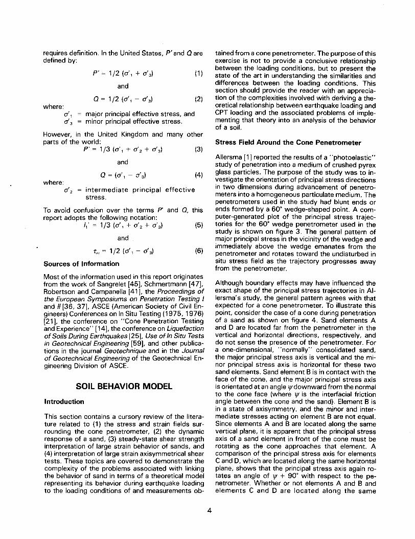
Allersma [1] reported the results of a "photoelastic"study of penetration into a medium of crushed pyrexglass particles. The purpose of the study was to in-vestigate the orientation of principal stress directionsin two dimensions during advancement of penetro-meters into a homogeneous particulate medium. Thepenetrometers used in the study had blunt ends orends formed by a 60. wedge-shaped point. A com-puter-generated plot of the principal stress trajec-tories for the 60. wedge penetrometer used in thestudy is shown on figure 3. The general pattern ofmajor principal stress in the vicinity of the wedge andimmediately above the wedge emanates from thepenetrometer and rotates toward the undisturbed insitu stress field as the trajectory progresses awayfrom the penetrometer.
(6)
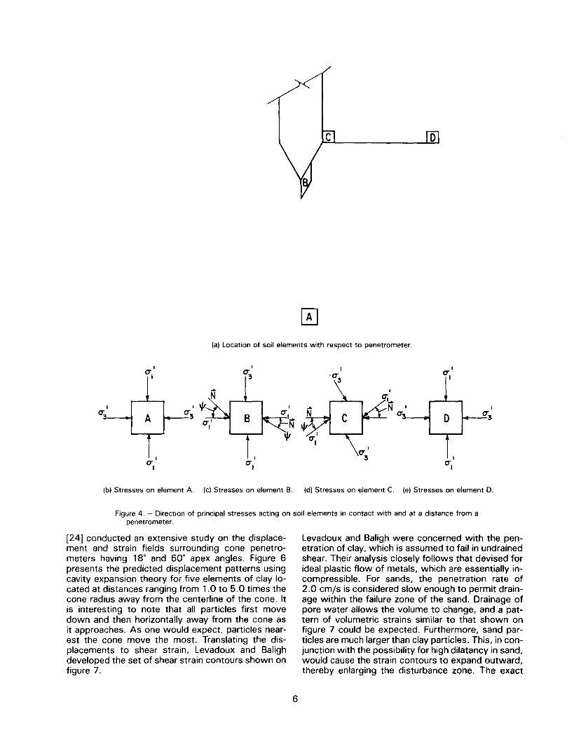
Although boundary effects may have influenced theexact shape of the principal stress trajectories in AI-lersma's study, the general pattern agrees with thatexpected for a cone penetrometer. To illustrate thispoint, consider the case of a cone during penetrationof a sand as shown on figure 4. Sand elements Aand D are located far from the penetrometer in thevertical and horizontal directions, respectively, anddo not sense the presence of the penetrometer. Fora one-dimensional, "normally" consolidated sand,the major principal stress axis is vertical and the mi-nor principal stress axis is horizontal for these twosand elements. Sand element B is in contact with theface of the cone, and the major principal stress axisis orientated at an angle Vldownward from the normalto the cone face (where VI is the interfacial frictionangle between the cone and the sand). Element B isin a state ofaxisymmetry, and the minor and inter-mediate stresses acting on element B are not equal.Since elements A and B are located along the samevertical plane, it is apparent that the principal stressaxis of a sand element in front of the cone must berotating as the cone approaches that element. Acomparison of the principal stress axis for elementsC and D, which are located along the same horizontalplane, shows that the principal stress axis again ro-tates an angle of VI + 90. with respect to the pe-netrometer. Whether or not elements A and Bandelements C and D are located along the same
4
, , , I
\ J..
,~\I
I \ J..I 1 .1
)0
x~)<:t
~'l:'i/'fi.J. "'f
.j.:Ji-
I.
'7
I I I
Xh'.H
y.
~
00~A/
x }£p 7".Y .J'...x: iI<xr,~Y¥X
. L-.J.-J
Figure 3. - Computer plot of the principal stress trajectories, based on 182 measuring points.From [1].
cipal stress trajectories depends on the stress levelinduced by the cone and the manner in which thesand surrounding the probe dissipates the stress field(i.e., it is entirely possible for a single stress trajec-tory beginning at the tip to terminate at the body ofthe penetrometer as shown on fig. 3).
Wroth [65] recognized the effect of the rotation ofthe principal stress axis on the behavior of soils andsuggested using the direct simple shear test insteadof the axisymmetrical triaxial compression shear test.He thought it more accurately modeled the stresspath to failure for the sand surrounding the cone pe-netrometer. This recommendation is based on theunderstanding that the simple shear test causes thestress path for a soil element to rotate from triaxialcompression at the beginning of a test to triaxial ex-tension at failure.
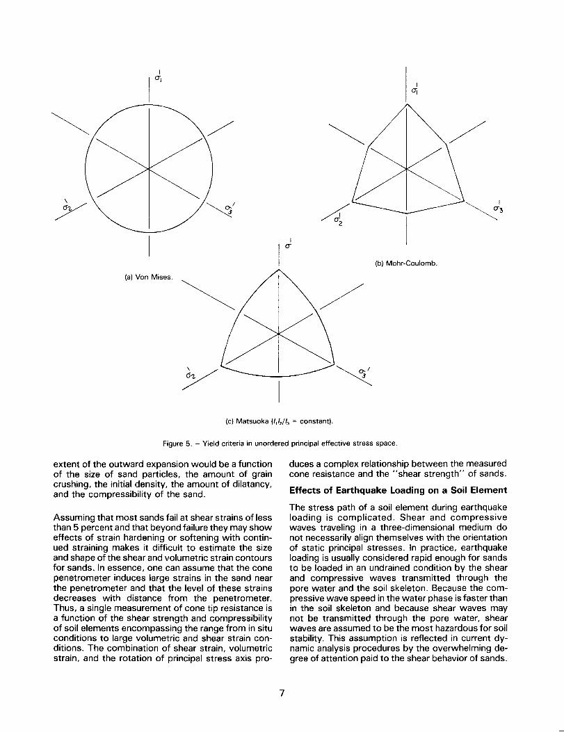
The importance of Wroth's recommendation can beillustrated with the aid of figure 5. If soils were tobehave according to the Von Mises yield criterion,the shear strength of the soil would be the same in
triaxial compression and triaxial extension. However,soils are usually assumed to behave according to theMohr-Coulomb criteria or more elaborate criteriasuch as the one devised by Matsuoka [28]. For bothof these yield criteria, the shear strength of the sandis less for any stress path to failure than it is for triaxialcompression, and the shear strength measured intriaxial extension forms the lower bound. Thus, se-lection of the shear strength from a test that causesthe soil to fail in triaxial extension would be a con-servative approach that would more accurately rep-resent the stress path to failure of a soil element nearthe penetrometer.
Strain Field Around the Cone Penetrometer
Little has been published about the displacement andstrain fields in sands surrounding the cone penetro-meter. To develop an understanding of the possibledisturbance effects of a penetrometer passingthrough a sand, a review of some of the work pub-lished on strain fields in clays surrounding the pe-netrometer must be performed. Levadoux and Baligh
5
,Oj~
N I I
B Ca:
D 0"3
0"'II
0",
I I0", 0"1
D
0(a) Location of soil elements with respect to penetrometer.
I0",
I
0"3
I
0"3 A
I
0"1
(b) Stresses on element A. (c) Stresses on element B.
I0"1
(d) Stresses on element C. (e) Stresses on element D.
Figure 4. - Direction of principal stresses acting on soil elements in contact with and at a distance from apenetrometer.
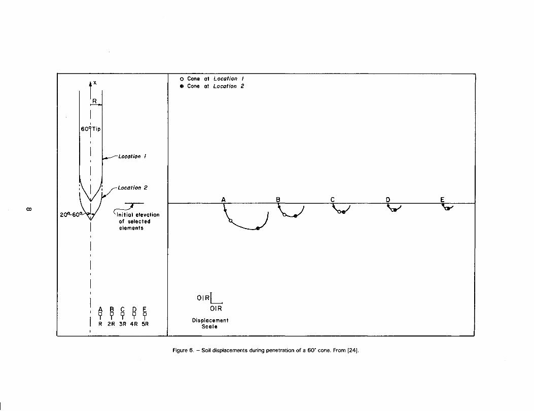
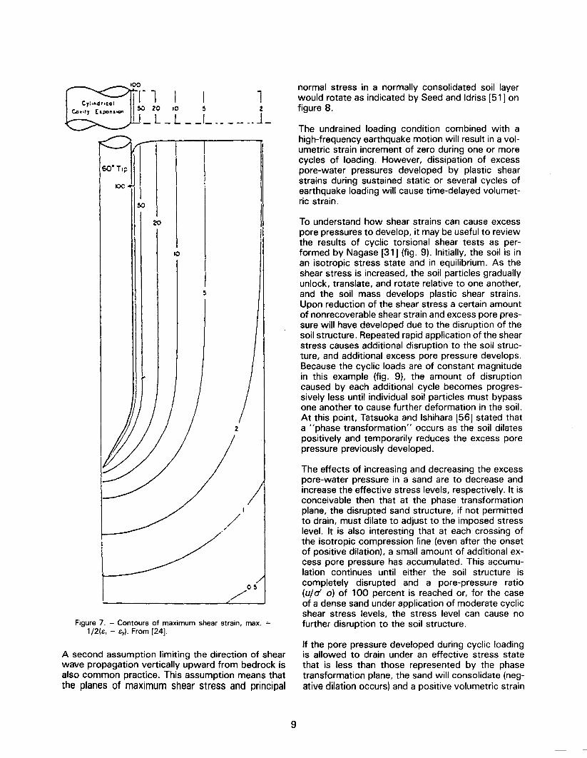
[24] conducted an extensive study on the displace-ment and strain fields surrounding cone penetro-meters having 18° and 60° apex angles. Figure 6presents the predicted displacement patterns usingcavity expansion theory for five elements of clay lo-cated at distances ranging from 1.0 to 5.0 times thecone radius away from the centerline of the cone. Itis interesting to note that all particles first movedown and then horizontally away from the cone asit approaches. As one would expect, particles near-est the cone move the most. Translating the dis-placements to shear strain, Levadoux and Balighdeveloped the set of shear strain contours shown onfigure 7.
Levadoux and Baligh were concerned with the pen-etration of clay, which is assumed to fail in undrainedshear. Their analysis closely follows that devised forideal plastic flow of metals, which are essentially in-compressible. For sands, the penetration rate of2.0 cmjs is considered slow enough to permit drain-age within the failure zone of the sand. Drainage ofpore water allows the volume to change, and a pat-tern of volumetric strains similar to that shown onfigure 7 could be expected. Furthermore, sand par-ticles are much larger than clay particles. This, in con-junction with the possibility for high dilatancy in sand,would cause the strain contours to expand outward,thereby enlarging the disturbance zone. The exact
6
I
I~
(-(Voo M;,,,
~
y
IOJ
/f'CT2
~3I
ICT
(b) Mohr-Coulomb.
~(c) Matsuoka (/,12/13 = constant).
Figure 5. - Yield criteria in unordered principal effective stress space.
extent of the outward expansion would be a functionof the size of sand particles, the amount of graincrushing, the initial density, the amount of dilatancy,and the compressibility of the sand.
Assuming that most sands fail at shear strains of lessthan 5 percent and that beyond failure they may showeffects of strain hardening or softening with contin-ued straining makes it difficult to estimate the sizeand shape of the shear and volumetric strain contoursfor sands. In essence, one can assume that the conepenetrometer induces large strains in the sand nearthe penetrometer and that the level of these strainsdecreases with distance from the penetrometer.Thus, a single measurement of cone tip resistance isa function of the shear strength and compressibilityof soil elements encompassing the range from in situconditions to large volumetric and shear strain con-ditions. The combination of shear strain, volumetricstrain, and the rotation of principal stress axis pro-
duces a complex relationship between the measuredcone resistance and the "shear strength" of sands.
Effects of Earthquake Loading on a Soil Element
The stress path of a soil element during earthquakeloading is complicated. Shear and compressivewaves traveling in a three-dimensional medium donot necessarily align themselves with the orientationof static principal stresses. In practice, earthquakeloading is usually considered rapid enough for sandsto be loaded in an undrained condition by the shearand compressive waves transmitted through thepore water and the soil skeleton. Because the com-pressive wave speed in the water phase is faster thanin the soil skeleton and because shear waves maynot be transmitted through the pore water, shearwaves are assumed to be the most hazardous for soilstability. This assumption is reflected in current dy-namic analysis procedures by the overwhelming de-gree of attention paid to the shear behavior of sands.
7
rR
I
I
6°1TiP
Location I
ex>
\~VLocation 2
200-600~ (Initi~ elevation
I
of selectedelements
ABC D E9 9 9 ? 9R 2R 3R 4R 5R
0 Cone at Location I. Cone at Location 2
OIRLOIR
DisplacementScale
E
Figure 6. - Soildisplacements during penetration of a 60. cone. From [24].
~
II
20
10
5
2
/
I
/"
05,,/
Figure 7. - Contours of maximum shear strain, max. =1/2(&, - Eo). From [24].
A second assumption limiting the direction of shearwave propagation vertically upward from bedrock isalso common practice. This assumption means thatthe planes of maximum shear stress and principal
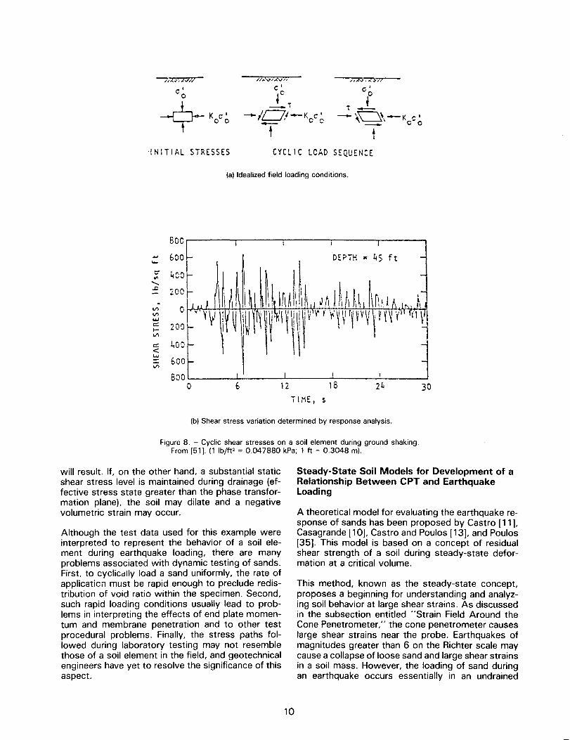
normal stress in a normally consolidated soil layerwould rotate as indicated by Seed and Idriss [51] onfigure 8.
The undrained loading condition combined with ahigh-frequency earthquake motion will result in a vol-umetric strain increment of zero during one or morecycles of loading. However, dissipation of excesspore-water pressures developed by plastic shearstrains during sustained static or several cycles ofearthquake loading will cause time-delayed volumet-ric strain.
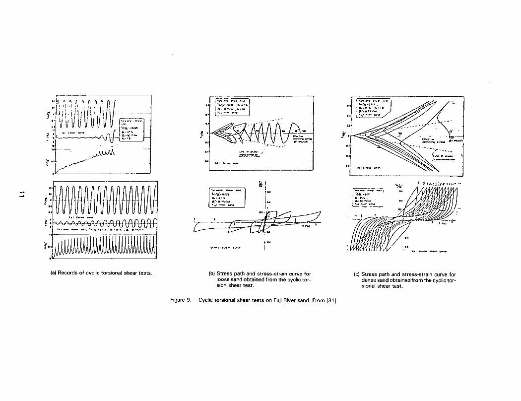
To understand how shear strains can cause excesspore pressures to develop, it may be useful to reviewthe results of cyclic torsional shear tests as per-formed by Nagase [31] (fig. 9). Initially, the soil is inan isotropic stress state and in equilibrium. As theshear stress is increased, the soil particles graduallyunlock, translate, and rotate relative to one another,and the soil mass develops plastic shear strains.Upon reduction of the shear stress a certain amountof nonrecoverable shear strain and excess pore pres-sure will have developed due to the disruption of thesoil structure. Repeated rapid application of the shearstress causes additional disruption to the soil struc-ture, and additional excess pore pressure develops.Because the cyclic loads are of constant magnitudein this example (fig. 9), the amount of disruptioncaused by each additional cycle becomes progres-sively less until individual soil particles must bypassone another to cause further deformation in the soil.At this point, Tatsuoka and Ishihara [56] stated thata "phase transformation" occurs as the soil dilatespositively and temporarily reduces the excess porepressure previously developed.
The effects of increasing and decreasing the excesspore-water pressure in a sand are to decrease andincrease the effective stress levels, respectively. It isconceivable then that at the phase transformationplane, the disrupted sand structure, if not permittedto drain, must dilate to adjust to the imposed stresslevel. It is also interesting that at each crossing ofthe isotropic compression line (even after the onsetof positive dilation), a small amount of additional ex-cess pore pressure has accumulated. This accumu-lation continues until either the soil structure iscompletely disrupted and a pore-pressure ratio(u/a' 0) of 100 percent is reached or, for the caseof a dense sand under application of moderate cyclicshear stress levels, the stress level can cause nofurther disruption to the soil structure.
If the pore pressure developed during cyclic loadingis allowed to drain under an effective stress statethat is less than those represented by the phasetransformation plane, the sand will consolidate (neg-ative dilation occurs) and a positive volumetric strain
9
800.., 600 DE?TH = ~S ft....
C"" 400VI........c 200
VI 0' .VI....,
~200to-VI
~~OO<....,
600=VI
800a (, 12 18 24 30
ilME, s
(b) Shear stress variation determined by response analysis.
0'0
-~KO'T- 00
//.,..v/~..,~,c't_T
-Jr-JI-K 0'fL...J; 0'"Tv
~~~
0'0. +,-
-'..~\.-K""\~\ c"'o
t
/,.i..-J.~"';"'/
INITIAL STRESSES CYCLIC LOAD SEQUENCE
(a) Idealized field loading conditions.
Figure 8. - Cyclic shear stresses on a soil element during ground shaking.From [51]. (1 Ib/ft> = 0.047880 kPa; 1 ft = 0.3048 m).
will result. If, on the other hand, a substantial staticshear stress level is maintained during drainage (ef-fective stress state greater than the phase transfor-mation plane), the soil may dilate and a negativevolumetric strain may occur.
Although the test data used for this example wereinterpreted to represent the behavior of a soil ele-ment during earthquake loading, there are manyproblems associated with dynamic testing of sands.First, to cyclically load a sand uniformly, the rate ofapplicaticil must be rapid enough to preclude redis-tribution of void ratio within the specimen. Second,such rapid loading conditions usually lead to prob-lems in interpreting the effects of end plate momen-tum and membrane penetration and to other testprocedural problems. Finally, the stress paths fol-lowed during laboratory testing may not resemblethose of a soil element in the field, and geotechnicalengineers have yet to resolve the significance of thisaspect.
Steady-State Soil Models for Development of aRelationship Between CPT and EarthquakeLoading
A theoretical model for evaluating the earthquake re-sponse of sands has been proposed by Castro [11],Casagrande [10], Castro and Poulos [13], and Poulos[35]. This model is based on a concept of residualshear strength of a soil during steady-state defor-mation at a critical volume.
This method, known as the steady-state concept,proposes a beginning for understanding and analyz-ing soil behavior at large shear strains. As discussedin the subsection entitled "Strain Field Around theCone Penetrometer," the cone penetrometer causeslarge shear strains near the probe. Earthquakes ofmagnitudes greater than 6 on the Richter scale maycause a collapse of loose sand and large shear strainsin a soil mass. However, the loading of sand duringan earthquake occurs essentially in an undrained
10
-"-"
r
r :t !\: r~
.i~i r
~
:~'
J\JV
'-. ----..
.'j' I, if II 'II
I
r::~~.. U II V V 1"/"".'"-': w'"
vV-I"''''~r~,~~-- -
~.:~
!~MWJM-~:. '''M~1VVtftf
(a) Records of cyclic torsional shear tests.
I ; ~. -. I., ."""4''''"
..,."I a.'.."""'..., ".t. I
... L:.::-- ~ J
.f
..
... L-"'~,.
~~~
.. .e,'"
~!I:'"
1 1.- ...,t./",', OlIO~.ct,
(1'.."\1'''''''..,,-......
.
~
to.I,
~~.-~-1- ,~J-
""-............-~o.I
(b) Stress path and stress-strain curve for
loose sand obtained from the cyclic tor-sion shear test.
Figure 9. - Cyclic torsional shear tests on Fuji River sand. From [31].
n. '~~ .-."" I.. 1./(1.'."" ..
D-.""" ...
~.o. (t '.tf u,/"",
... l '"'''--'''''
..1 .... !~.
~~ ..~ Ct"1-vaJi.,~
I:r (.)
''''U'...,..
(c) Stress path and stress-strain curve fordense sand obtained from the cyclic tor-sional shear test.
(constant volume) mode, whereas the cone penetro-meter loading in sands occurs in a drained mode. Toconceptually relate the two loading paths, a largestrain soil model is required.
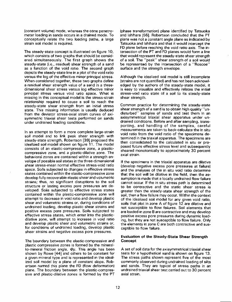
The steady-state concept is illustrated on figure 10,which consists of two graphs that should be consid-ered simultaneously. The first graph shows thesteady-state (i.e., residual) shear strength of a sandas a function of the void ratio. The second graphdepicts the steady-state line in a plot of the void ratioversus the log of the effective minor principal stress.When considered together, these two graphs definea residual shear strength value of a sand in a three-dimensional shear stress versus log effective minorprincipal stress versus void ratio space. What ismissing in this conceptual model is the stress-strainrelationship required to cause a soil to reach thesteady-state shear strength from an initial stressstate. This missing information is usually deducedfrom the deviator stress-axial strain curves of axi-symmetric triaxial shear tests performed on sandsunder undrained loading conditions.
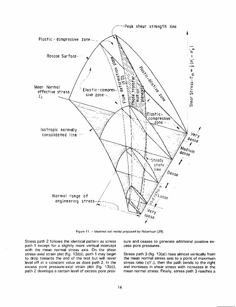
In an attempt to form a more complete large-strainsoil model and to link peak shear strength withsteady-state strength, Robertson [39] proposed theidealized soil model shown on figure 11. The modelconsists of an elastic-compressive zone, a plastic-compressive zone, and a plastic-dilative zone. Thebehavioral zones are contained within a strength en-velope of possible soil states inthe three-dimensionalshear stress-mean normal effective stress-void ratiospace. Soils subjected to changes in effective stressstates contained within the elastic-compressive zonedevelop fullyrecoverable elastic shear and volumetricstrains; thus, no significant disruptions to the soilstructure or lasting excess pore pressures are de-veloped. Soils subjected to effective stress statescontained within the plastic-compressive zone willattempt to decrease in void ratio and develop plasticshear and volumetric strains or, during conditions ofundrained loading, develop plastic shear strains andpositive excess pore pressures. Soils subjected toeffective stress states, which enter into the plastic-dilative zone, will attempt to increase in void ratioand develop plastic shear and volumetric strains or,for conditions of undrained loading, develop plasticshear strains and negative excess pore pressures.
The boundary between the elastic-compressive andplastic compressive zones is formed by the mineral-to-mineral friction angle, l1>J1..This angle has beenshown by Rowe [44] and others to be constant fora given mineral type and is represented in the ideal-ized soil model by a plane of constant slope. Rob-ertson named this plane the FD (flow deformation)plane. The boundary between the plastic-compres-sive and plastic-dilative zones is formed by the PT
(phase transformation) plane identified by Tatsuokaand Ishihara [56]. Robertson concluded that the PTplane was not a constant angle plane as indicated byTatsuoka and Ishihara and that it would intercept theFD plane before reaching the void ratio axis. The in-tersection of the PT and FD planes would form a linethat would represent the steady-state shear strengthof a soil. The "peak" shear strength of a soil wouldbe represented by the intersection of a "Roscoe"surface and the strength envelope.
Although the idealized soil model is still incomplete(strains are not quantified) and has not been acknowl-edged by the authors of the steady-state model, itis easy to visualize and effectively relates the initialstress-void ratio state of a soil to its steady-stateshear strength.
Common practice for determining the steady-stateshear strength of a sand is to obtain high quality "un-disturbed" samples of sands and test them in anaxisymmetrical triaxial shear apparatus under un-drained conditions. Before and after sampling, trans-porting, and handling of the samples, carefulmeasurements are taken to back-calculate the in situvoid ratio from the void ratio of the specimens de-termined in the triaxial apparatus. The specimens arethen consolidated to the calculated in situ or pro-posed future effective stress level and subsequentlysheared monotonically to approximately 30 percentaxial strain.
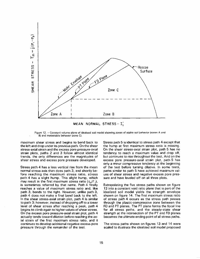
If the specimens in the triaxial apparatus are dilative(develop negative excess pore pressures at failure)and the analyses of the in situ void ratio determinethat the soil will be dilative in the field, then the as-sumption is made that a locally undrained flow failurecannot occur. If the in situ stress path is determinedto be contractive and the static shear stress isgreater than the steady-state shear strength of thesoil, then a flow failure may occur. Within the contextof the idealized soil model for any given void ratio,soils that plot in zone A of figure 12 are dilative andnot susceptible to flow failures. Soil elements thatare loaded in zone B are contractive and may developpositive excess pore pressures during dynamic load-ing, but they are not susceptible to flow failure. Onlythe elements in zone C are both contractive and sus-ceptible to flow failure.
Evaluation of the Steady-State Shear StrengthConcept
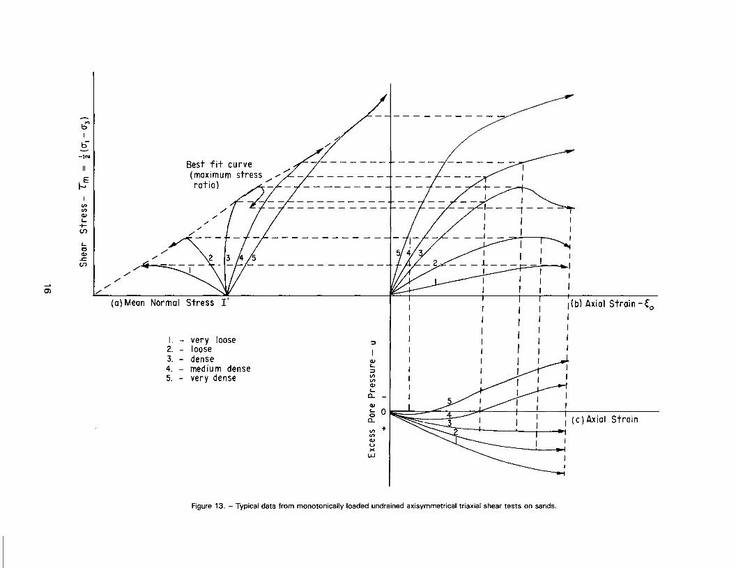
A set of soil data for the axisymmetrical triaxial sheartests for a hypothetical sand is shown on figure 13.The stress paths shown represent five of the mostcommonly observed during undrained loading of siltsand sands. They are typical of stress paths in anundrained triaxial shear test carried out to 30 percentaxial strain.
12
otI
bI0-
-INIIE
I-->
IenencuL+-(f)
L0CU
~(f)
- otI
b0'10
J
lineSteady - state
Void Ratio - e
~.5'1-
e()Q'')1',
$1-()1-
eIiI)
e
Void Ratio - e
Figure 10. - Steady-state soil modei.
Figure 13 shows that the stress paths for this hy-pothetical soil indicate a distinct pattern for each ofthe five placement void ratios when the soil is iso-tropically consolidated to the same mean normalstress. Path 1, which is at the highest void ratio, be-gins to generate positive pore pressures (fig. 13(c))at the slightest increment of shear stress and con-tinues to generate additional positive pore pressures
throughout the test. On the stress space plot, path 1moves immediately through lower levels of mean nor-mal stress with increases in the shear stress until apeak shear stress is reached. From the peak shearstress, path 1 will either begin to drop in both shearstress and mean normal stress until the test isterminated, or, as shown, path 1 will reach a peakshear stress and remain there to the end of the test.
13
Normal range ofengineering stress-
Peak shear strength line
Plastic - compressive zone----_-~,,
,-
Roscoe Surface-.
- '"IbI
b-
Mean Norma Ieffective stress1'2
-INIIE
I-->I
~In(1)
'-+-CfJ
'-0(1)
..s:::.,CfJ
Isotropic normallyconsolidated Iine-/
I. - ~~ Ve/'y
.
denseI
;'ediurnenseI
I
Figure 11. - Idealized soil model proposed by Robertson [39].
Stress path 2 follows the identical pattern as stresspath 1 except for a slightly more vertical interceptwith the mean normal stress axis. On the shearstress-axial strain plot (fig. 13(b)), path 1 may beginto drop towards the end of the test but will neverlevel off at a constant value as does path 2. In theexcess pore pressure-axial strain plot (fig. 13(c)),path 2 develops a certain level of excess pore pres-
sure and ceases to generate additional positive ex-cess pore pressures.
Stress path 3 (fig. 13(a)) rises almost vertically fromthe mean normal stress axis to a point of maximumstress ratio (Tfl',), then the path bends to the rightand increases in shear stress with increases in themean normal stress. Finally, stress path 3 reaches a
14
~I
b-IN
II
~I
Cf)Cf)Wa::t-Cf)
a::<tw:I:Cf) Zone C
------------------
Zone B
MEAN NORMALSTRESS- r;
Figure 12. - Constant volume plane of idealized soil model showing zones of stable soil behavior (zones A andB) and metastable behavior (zone C).
maximum shear stress and begins to bend back tothe left and drop under its previous path. On the shearstress-axial strain and the excess pore pressure-axialstrain plots, paths 2 and 3 follow almost identicaltrends, the only differences are the magnitudes ofshear stress and excess pore pressure developed.
Stress path 4 has a less vertical rise from the meannormal stress axis than does path 3, and shortly be-fore reaching the maximum stress ratio, stresspath 4 has a slight hump. This slight hump, whichmay result in the first maximum stress ratio (.mll' ,),is sometimes referred by that name. Path 4 finallyreaches a value of maximum stress ratio and, likepath 3, bends to the right. However, unlike path 3,path 4 does not make a final bend back to the left.In the shear stress-axial strain plot, path 4 is similarto path 3; however, instead of dropping off to a lowerlevel of shear stress after reaching a peak, path 4begins to climb again to higher values of shear stress.On the excess pore pressure-axial strain plot, path 4actually tends toward dilation before reaching the ax-ial strain of the first maximum stress ratio, and itcontinues to develop additional negative excess porepressure through the remainder of the test.
Stress path 5 is identical to stress path 4 except thatthe hump at first maximum stress ratio is missing.On the shear stress-axial strain plot, path 5 has notendency to reach a maximum value and drop off,but continues to rise throughout the test. And on theexcess pore pressure-axial strain plot, path 5 hasonly a minor compressive tendency at the beginningof the test before turning dilative. In some tests,paths similar to path 5 have achieved maximum val-ues of shear stress and negative excess pore pres-sure and have leveled off on all three plots.
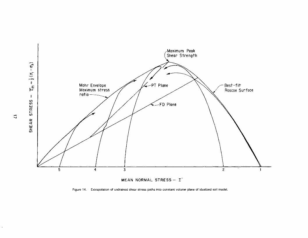
Extrapolating the five stress paths shown on figure13 into a constant void ratio plane that is part of theidealized soil model yields the strength envelopeshown on figure 14. The first maximum stress ratioof stress path 4 occurs as the stress path passesthrough the plastic-compressive zone between theFD and PT planes. The PT plane forms the focal linefor all stress paths, and the steady-state shearstrength at the intersection of the PT and FD planesbecomes the ultimate ending point of all stress paths.
The stress paths shown on figures 13 and 14 werescaled to illustrate the idealized soil model proposed
15
b'I
b--IN
~IfJ)fJ)c»I...
+-(f)
I...Cc»
.r:(f)
a>
(0) Mean Normal Stress I'
././
././
-----------
Best fit curve(maximum stress",./ratio) ./
./
'"
I. - very loose2. - loose3. - dense4. - medium dense5. - very dense
I,
IIIIII
,(b) Axial Strain -~o
III,
:J
c»I...::JfJ)fJ)c»I...a.. -c»2; 0a..
V'J +fJ)c»uxW
Figure 13. - Typical data from monotonically loaded undrained axisymmetrical triaxial shear tests on sands.
~I
b-
-INII
Mohr Envelope~Maximum stress
I ratio(/)(/)
wa:::I-(/)
-...Ja:::<[wI(/)
5 24 3
MEAN NORMAL STRESS - I'
Figure 14. - Extrapolation of undrained shear stress paths into constant volume plane of idealized soil model.
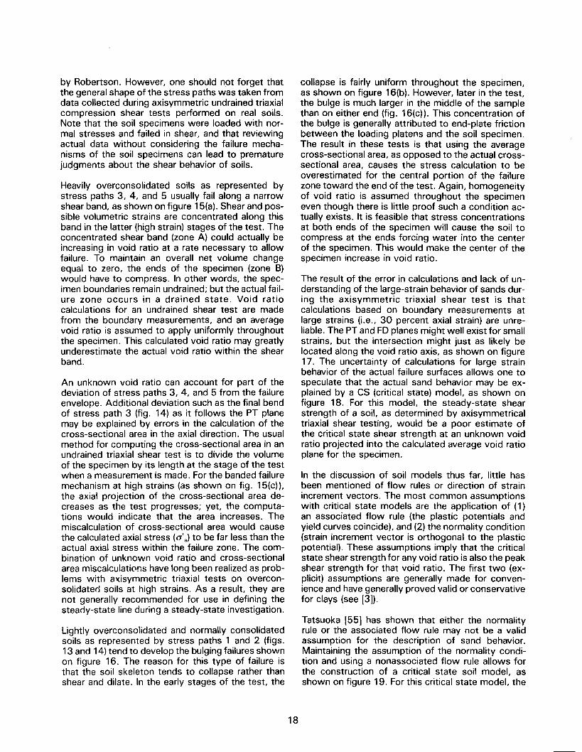
by Robertson. However, one should not forget thatthe general shape of the stress paths was taken fromdata collected during axisymmetric undrained triaxialcompression shear tests performed on real soils.Note that the soil specimens were loaded with nor-mal stresses and failed in shear, and that reviewingactual data without considering the failure mecha-nisms of the soil specimens can lead to prematurejudgments about the shear behavior of soils.
Heavily overconsolidated soils as represented bystress paths 3, 4, and 5 usually fail along a narrowshear band, as shown on figure 15(a). Shear and pos-sible volumetric strains are concentrated along thisband in the latter (high strain) stages of the test. Theconcentrated shear band (zone A) could actually beincreasing in void ratio at a rate necessary to allowfailure. To maintain an overall net volume changeequal to zero, the ends of the specimen (zone B)would have to compress. In other words, the spec-imen boundaries remain undrained; but the actual fail-ure zone occurs in a drained state. Void ratiocalculations for an undrained shear test are madefrom the boundary measurements, and an averagevoid ratio is assumed to apply uniformly throughoutthe specimen. This calculated void ratio may greatlyunderestimate the actual void ratio within the shearband.
An unknown void ratio can account for part of thedeviation of stress paths 3, 4, and 5 from the failureenvelope. Additional deviation such as the final bendof stress path 3 (fig. 14) as it follows the PT planemay be explained by errors in the calculation of thecross-sectional area in the axial direction. The usualmethod for computing the cross-sectional area in anundrained triaxial shear test is to divide the volumeof the specimen by its length at the stage of the testwhen a measurement is made. For the banded failuremechanism at high strains (as shown on fig. 15(c)),the axial projection of the cross-sectional area de-creases as the test progresses; yet, the computa-tions would indicate that the area increases. Themiscalculation of cross-sectional area would causethe calculated axial stress (da) to be far less than theactual axial stress within the failure zone. The com-bination of unknown void ratio and cross-sectionalarea miscalculations have long been realized as prob-lems with axisymmetric triaxial tests on overcon-solidated soils at high strains. As a result, they arenot generally recommended for use in defining thesteady-state line during a steady-state investigation.
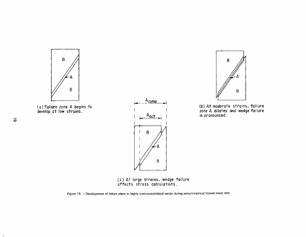
Lightly overconsolidated and normally consolidatedsoils as represented by stress paths 1 and 2 (figs.13 and 14) tend to develop the bulging failures shownon figure 16. The reason for this type of failure isthat the soil skeleton tends to collapse rather thanshear and dilate. In the early stages of the test, the
collapse is fairly uniform throughout the specimen,as shown on figure 16(b). However, later in the test,the bulge is much larger in the middle of the samplethan on either end (fig. 16(c)). This concentration ofthe bulge is generally attributed to end-plate frictionbetween the loading platens and the soil specimen.The result in these tests is that using the averagecross-sectional area, as opposed to the actual cross-sectional area, causes the stress calculation to beoverestimated for the central portion of the failurezone toward the end of the test. Again, homogeneityof void ratio is assumed throughout the specimeneven though there is little proof such a condition ac-tually exists. It is feasible that stress concentrationsat both ends of the specimen will cause the soil tocompress at the ends forcing water into the centerof the specimen. This would make the center of thespecimen increase in void ratio.
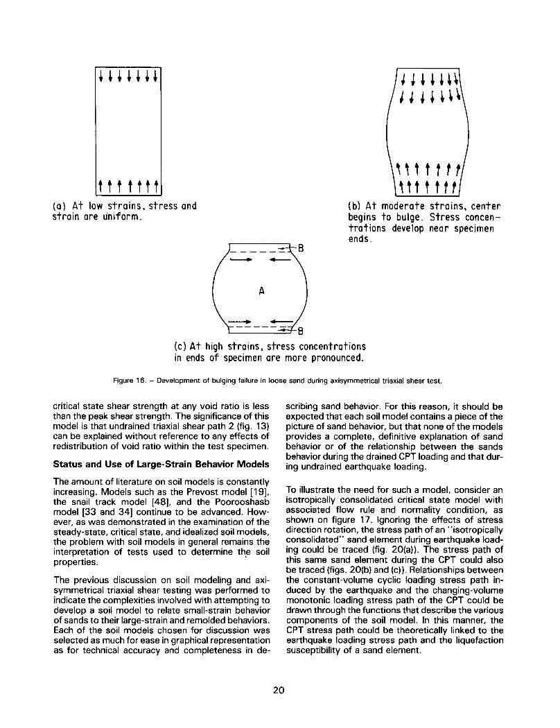
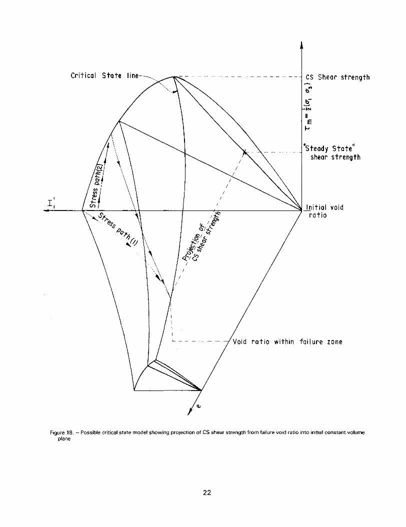
The result of the error in calculations and lack of un-derstanding of the large-strain behavior of sands dur-ing the axisymmetric triaxial shear test is thatcalculations based on boundary measurements atlarge strains (i.e., 30 percent axial strain) are unre-liable. The PT and FDplanes might well exist for smallstrains, but the intersection might just as likely belocated along the void ratio axis, as shown on figure17. The uncertainty of calculations for large strainbehavior of the actual failure surfaces allows one tospeculate that the actual sand behavior may be ex-plained by a CS (critical state) model, as shown onfigure 18. For this model, the steady-state shearstrength of a soil, as determined by axisymmetricaltriaxial shear testing, would be a poor estimate ofthe critical state shear strength at an unknown voidratio projected into the calculated average void ratioplane for the specimen.
In the discussion of soil models thus far, little hasbeen mentioned of flow rules or direction of strainincrement vectors. The most common assumptionswith critical state models are the application of (1)an associated flow rule (the plastic potentials andyield curves coincide), and (2) the normality condition(strain increment vector is orthogonal to the plasticpotential). These assumptions imply that the criticalstate shear strength for any void ratio is also the peakshear strength for that void ratio. The first two (ex-plicit) assumptions are generally made for conven-ience and have generally proved valid or conservativefor clays (see [3]).
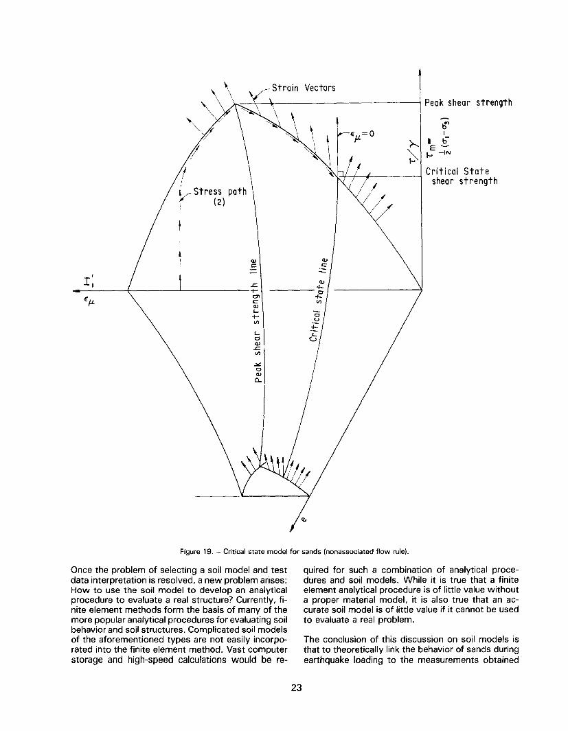
Tatsuoka [55] has shown that either the normalityrule or the associated flow rule may not be a validassumption for the description of sand behavior.Maintaining the assumption of the normality condi-tion and using a non associated flow rule allows forthe construction of a critical state soil model, asshown on figure 19. For this critical state model, the
18
B
B
I.. Acomp ..I( a) Failure zone A begins todevelop at low strains.
~ Aact---Ico
B
(c) At large strains. wedge failureaffects stress calculations.
B
B
(b) At moderate strains. fai lurezone A di lates and wedge fai lureis pronounced.
Figure 15. - Development of failure plane in highly overconsolidated sands during axisymmetrical triaxial shear test.
..+++++
ttttttt(a) At low strains, stress andstrain are uniform.
J.+.+.~JJ~.+~\
"'tttf"ttttt
(b) At moderate strains, centerbegins to bulge. Stress concen-trations develop near specimenends.
8(c) At high strains. stress concentrationsin ends of specimenore more pronounced.
Figure 16. - Development of bulging failure in loose sand during axisymmetrical triaxial shear test.
critical state shear strength at any void ratio is lessthan the peak shear strength. The significance of thismodel is that undrained triaxial shear path 2 (fig. 13)can be explained without reference to any effects ofredistribution of void ratio within the test specimen.
Status and Use of Large-Strain Behavior Models
The amount of literature on soil models is constantlyincreasing. Models such as the Prevost model [19],the snail track model [48], and the Poorooshasbmodel [33 and 34] continue to be advanced. How-ever, as was demonstrated in the examination of thesteady-state, critical state, and idealized soil models,the problem with soil models in general remains theinterpretation of tests used to determine th.e soilproperties.
The previous discussion on soil modeling and axi-symmetrical triaxial shear testing was performed toindicate the complexities involved with attempting todevelop a soil model to relate small-strain behaviorof sands to their large-strain and remolded behaviors.Each of the soil models chosen for discussion wasselected as much for ease in graphical representationas for technical accuracy and completeness in de-
scribing sand behavior. For this reason, it should beexpected that each soil model contains a piece of thepicture of sand behavior, but that none of the modelsprovides a complete, definitive explanation of sandbehavior or of the relationship between the sandsbehavior during the drained CPT loading and that dur-ing undrained earthquake loading.
To illustrate the need for such a model, consider anisotropically consolidated critical state model withassociated flow rule and normality condition, asshown on figure 17. Ignoring the effects of stressdirection rotation, the stress path of an "isotropicallyconsolidated" sand element during earthquake load-ing could be traced (fig. 20(a)). The stress path ofthis same sand element during the CPT could alsobe traced (figs. 20(b) and (c)). Relationships betweenthe constant-volume cyclic loading stress path in-duced by the earthquake and the changing-volumemonotonic loading stress path of the CPT could bedrawn through the functions that describe the variouscomponents of the soil model. In this manner, theCPT stress path could be theoretically linked to theearthquake loading stress path and the liquefactionsusceptibility of a sand element.
20
Mean NormalEffective Stress
I;
b'"I
b-
-IN
"Ef-J({)({)
wa:::f-({)
a:::ctw:I:({)
Flow Deformation Plane
Isotropic NormalConsolidationLine
cz,
/.0
-i::G?
.~....~
Figure 17. - Critical state soil model for sands.
21
I
II
Critical State line CS Shear strengthbrt'l
£-IN
IIE
I--
."Steady State
shear strength
Initial voidratio
Void ratio within fai I ure zone
Figure 18. - Possible critical state model showing projection of CS shear strength from failure void ratio into initial constant volumeplane.
22
Q) Q)
c c:-I
II .£:;+-
€fL0>CQ)
'-+-cJ)
'-0Q).£:;cJ)
~0Q)
a..
Strain Vectors
f
!~.-rStress pathr (2)
Peak shear strength
b'"I
'- II b-r-. E-~ -IN....
Critical Stateshear strength
Figure 19. - Critical state model for sands (nonassociated flow rule).
Once the problem of selecting a soil model and testdata interpretation is resolved, a new problem arises:How to use the soil model to develop an analyticalprocedure to evaluate a real structure? Currently, fi-nite element methods form the basis of many of themore popular analytical procedures for evaluating soilbehavior and soil structures. Complicated soil modelsof the aforementioned types are not easily incorpo-rated into the finite element method. Vast computerstorage and high-speed calculations would be re-
quired for such a combination of analytical proce-dures and soil models. While it is true that a finiteelement analytical procedure is of little value withouta proper material model, it is also true that an ac-curate soil model is of little value if it cannot be usedto evaluate a real problem.
The conclusion of this discussion on soil models isthat to theoretically link the behavior of sands duringearthquake loading to the measurements obtained
23
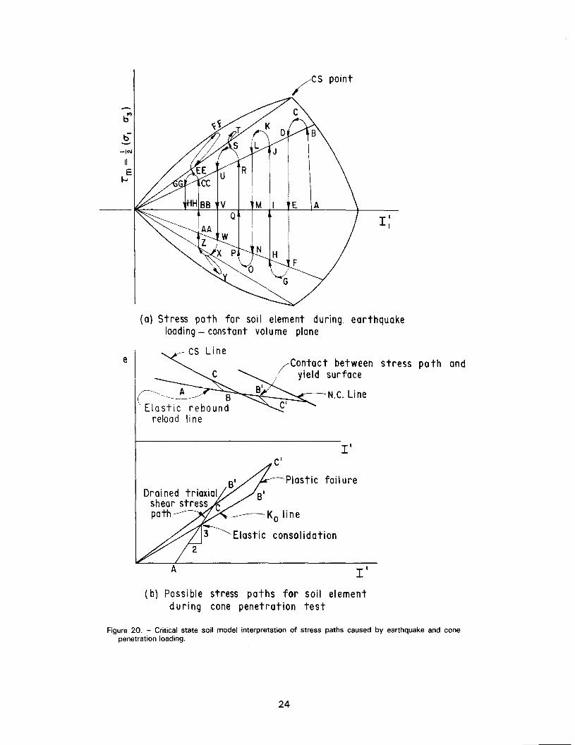
/CS point
b-
III
b'"
-INIIE
j...
(a) Stress path for soil element during, earthquakeloading - constant volume plane
e (Contact between stress path and
/ yield surface
-N.C. Line
II
Drai ned triaxialshear stress Cpath Ko line
~Elastic consolidation2
Plastic fail ure
II
(b) Possible stress paths for soil elementduring cone penetration test
Figure 20. - Critical state soil model interpretation of stress paths caused by earthquake and conepenetration loading.
24
during the cone penetration test requires a realisticsoil model. a procedure for obtaining the soil param-eters to describe the soil model, and a computer anal-ysis capable of implementing the soil model.Currently, an abundance of soil models exists, buttheir accuracy in relating the large-strain drained be-havior to the undrained behavior of a sand is ques-tionable. Finite element computer analysisprocedures are limited in their ability to handle. manyof the proposed soil models by the ne~esslty fo.rlarge-memory, high-speed computers. FIn~lIy, so~1tests to determine the properties that descnbe a sOilmodel are either nonexistent or are in research anddevelopment stages and not available to the entireengineering community. Thus, the primary nee.ds ~ora complete large-strain soil model are (1) qualitativeevaluation of the limitations of current analytical tech-niques; and (2) proper selection of soil parametersfor developing empirical relationships. The latterneed is demonstrated in the section entitled "ConePenetration Practice."
Additional Problems with Association of ConePenetration Testing to Earthquake Responseof Soils
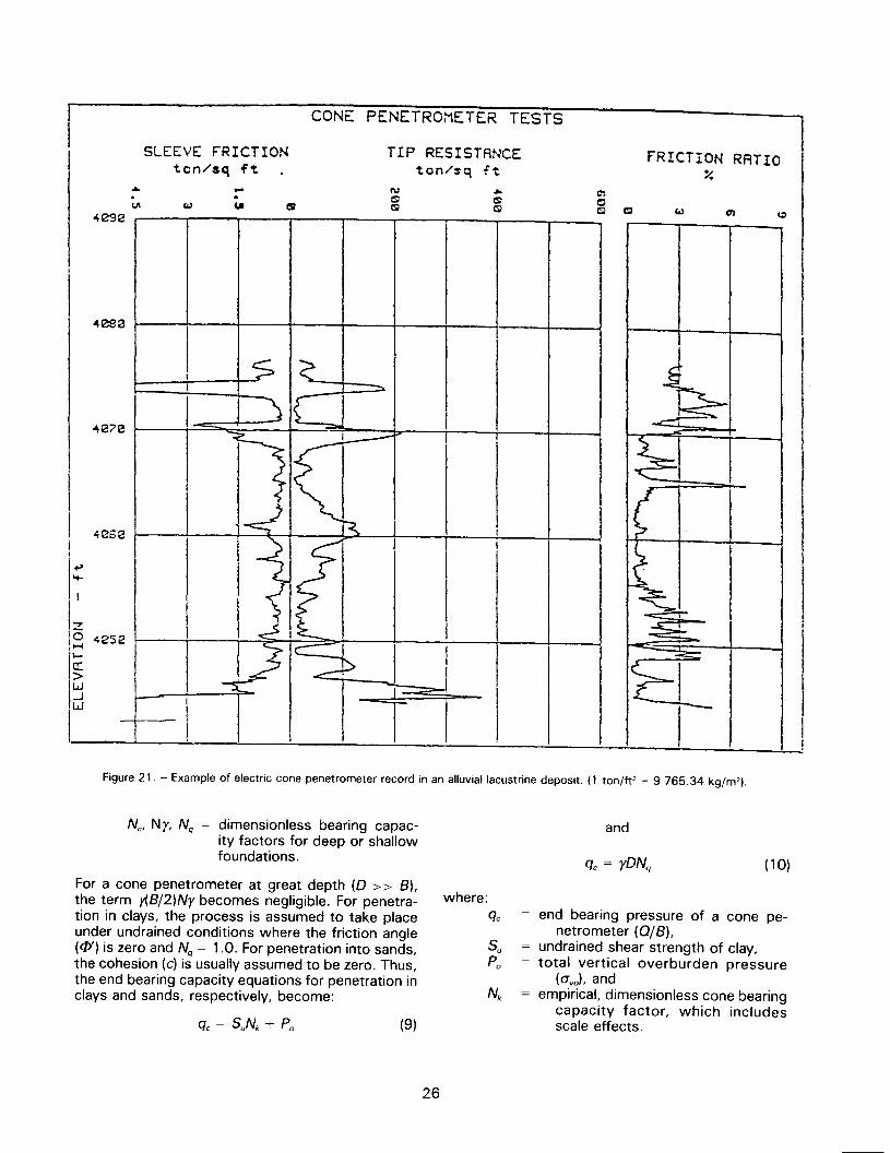
Additional problems associated with application of atheoretical relationship between CPT loading andearthquake loading of real soil deposits arise fromthe nature of these deposits. Seldom is a real ho-mogeneous clean sand deposit of several feet inthickness encountered. Cone penetration tests per-formed in areas of alluvial-lacustrine deposits aregenerally spiked with peaks and valleys, as .shownon figure 21. In deposits of gravel. sand, silt, andclay, continuous profiles from one sounding hole tothe next are difficult to correlate, and layers are sothin that assuming the full failure strength of a layeris developed during the CPT is highly misleading.Even for soils deposited in a deltaic environment, thinseasonal layering is evident. Guidelines related to thethickness of a layer required before full end bearingresistance is developed within that layer have beenproposed by Schmertmann [47], Robertson andCampanella [41], and others. A general rule of thumbof approximately 15 cone diameters (0.5 m) is oftenused. Thus, the use of theoretical models and ana-lytical procedures for interpretation of CPT data forreal soil deposits always requires some degree ofexperience and judgment on the part of the engineer.
In addition to the problems related to the layering ofreal soil deposits, the drainage condition of real soilsis seldom known during performance of the CPT. Theassumptions of drained failure for clean sands andundrained failure for clays during the CPT may bejustified, but questions remain on (1) the drainagecondition during CPT sounding insilty or clayey sandsand gravels, and (2) whether earthquake-related
structural problems are only limited to sands andgravels.
CONE PENETRATION THEORY
Introduction
Theoretical modeling and interpretation of CPT datahave developed primarily in terms of limit equilibriumand limitplasticity, and pragmatically in terms ?f gen-eral bearing capacity theory [17, 23] or cavity .ex-pansion theory [5, 60]. While some theoreticaladvancements have recently been proposed alongthe lines of strain path methods, which are based onideal plastic flow concepts [24], a significant amountof current research in this area has focused on claysnot generally susceptible to liquefaction during earth-quake loading. Therefore, this section concentrateson the limit equilibrium theories.
General Bearing Capacity Theory
The CPT was originally developed as a tool for piledesign. The cone penetrometer itself was .assumedto be a model pile; therefore, early analytical tech-niques for interpreting CPT data develope? from ~on-cepts used to analyze the bearing capacity of piles.Using equations of the same form to interprete n:'°deland prototype piles provided the added convemenceof lumping the effects of differences in ~nd beari~~,skin friction, and insertion rate into a single empln-cally derived scale effect parameter.
Pile load design is based on two components of re-sistance, skin friction (f) and end bearing (q). By as-suming uncoupled contributions from the twocomponents, the total pile load capacity (Q) may becalculated by superposition as:
Q = qAe + fAs (7)
where:AeAs
= end area of pile, and= side area of pile.
Buisman [8] and Terzaghi [57] proposed ~ generalequation for bearing capacity in the following form:
Q 8
£i=q = eNc + y (2) Ny + yDNq (8)
where:8 = base width or diameter,y = total unit weight of soil,0 = embedment depth,e = cohesion, or cohesive strength
of soil. and
25
I
CONt.. PENETROMETER TESTS
SLEEVE FRICTION TIP RESISTANCE FRICTION RATIOton/aq f't ton/$q ft %. - N . C). . ~~0UI
""... CSI ~Q
0Q
""~ege en I.:)
I
I
~ooe
"te?e~
I
I 4esei
I:j0 425 e'H
I~I~,W
Figure 21. - Example of electric cone penetrometer record in an alluvial lacustrine deposit. (1 ton/ft2= 9765.34 kg/m2).
Nc' Ny, Nq = dimensionless bearing capac-ity factors for deep or shallowfoundations.
and
qc = yONq (10)For a cone penetrometer at great depth (0 > > B).the term y(B/2)Ny becomes negligible. For penetra-tion in clays, the process is assumed to take placeunder undrained conditions where the friction angle(CP')is zero and Nq = 1.0. For penetration into sands,the cohesion (c) is usually assumed to be zero. Thus,the end bearing capacity equations for penetration inclays and sands, respectively, become:
where:qc
SuPo
= end bearing pressure of a cone pe-netrometer (O/B).
= undrained shear strength of clay,= total vertical overburden pressure
(avo).and= empirical, dimensionless cone bearing
capacity factor, which includesscale effects.
Nk
qc = SuNk + Po (9)
26
The skin friction component of pile capacity is oftenassumed to be proportional to the undrained shearstrength of a clay or the drained friction angle (<P')ofsands. The general forms of the equations that de-scribe skin adhesion and friction components of coneresistance for clay and sand, respectively, are:
Su = afs (11 )
and
<P' =(tan-1,8) fs
yB
(12)
where:a, ,8 = dimensionless cone correlation fac-
tors, andfs = cone friction sleeve measurement.
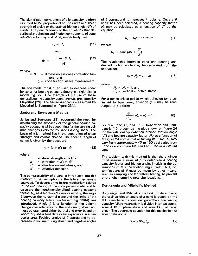
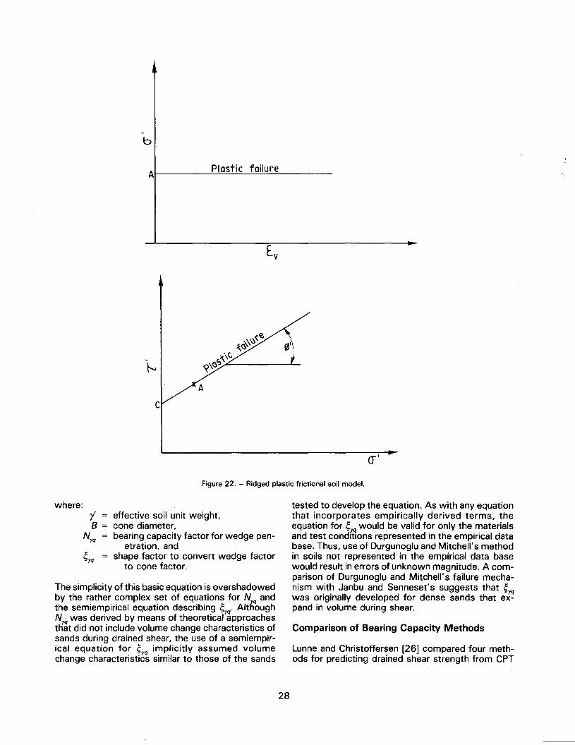
The soil model most often used to describe shearbehavior for bearing capacity theory is a rigid plasticmodel (fig. 22). One example of the use of thesegeneral bearing capacity equations was presented byMeyerhof [29]. The failure mechanism assumed byMeyerhof is illustrated on figure 23(a).
Janbu and Senneset's Method
Janbu and Senneset [23] recognized the need formaintaining the simplicity of the general bearing ca-pacity equations while accounting for the varying vol-ume changes exhibited by sands during shear. Thebasis of this method lies in the separation of shearstrength and volume change. The shear strength ofsands is given by the equation:
'Cf= (a + 0') tan <P' (13)
where:'Cfaa'c'
= shear strength at failure,= attraction = c' cot <P',
effective normal stress, and= effective cohesion.
The compressibility of a sand is introduced into thismethod in the description of the failure mechanismanalyzed. To describe the failure mechanism relatedto the end bearing of the cone penetrometer and tocalculate the nondimensionalized bearing capacityfactor, Nq,as a function of compressibility, the angle,8 between the horizontal plane and the limits of thebearing capacity failure mechanism (fig. 23(b)) wasintroduced. Angle ,8 is a function of the volumechange characteristics of the soil during shear andmust be estimated either by trial and error based onlaboratory shear test data or by experience in a par-ticular area. Positive angles of ,8 correspond to de-creases in volume during shear, and negative angles
of ,8 correspond to increases in volume. Once a ,8angle has been selected, a bearing capacity factorNq may be calculated as a function of <P' by theequation:
Nq = N,e (lr- 2 tHan <P') (14)
where:
<P'Nf = tan2 (45 + -)
2
The relationship between cone end bearing anddrained friction angle may be calculated from theexpression:
qc = Np(o'vo + a) (15)
where:Np = Nq - 1, and
o'vo = vertical effective stress.
For a cohesionless soil in which adhesion (a) is as-sumed to equal zero, equation (15) may be rear-ranged to the form:
qc-= N = N - 1, p q(j
vo
(16)
For ,8 = -15°, 0°, and +15°, Robertson and Cam-panella [40] presented the plot shown on figure 24for the relationship between drained friction angle(<P')and bearing capacity factor (Nq)as a function of,8. Figure 24 shows that assuming <P'= 42°, Nqmayvary from approximately 40 to 150 as ,8varies from+ 15° in a compressible sand to -15° in a dilatantsand.
The problem with this method is that the engineermust assume a value of ,8 to determine a bearingcapacity factor and friction angle. Implicit in the as-sumption of ,8 is the friction angle itself. Thus, de-terminations of ,8 must be made by other means,such as sampling and laboratory testing, to preventerrors when entering new site locations.
Durgunoglu and Mitchell's Method
Durgunoglu and Mitchell's method for determiningthe drained friction angle of a sand is based on thefailure mechanism shown on figure 23(c). The bearingcapacity failure mechanism is divided into two zones:zone AOC of plane shear and zone COE of radialshear. The governing equation for this mechanism ofshear behavior is:
- 'BNj:.q - Y rq~rq (17)
27
b
A Plastic failure
tv
h
.\.~~'G.Ii.~\\.
~\c,~\~C:,
0-'
where:
Figure 22. - Ridged plastic frictional soil model.
r' = effective soil unit weight,B = cone diameter,
Nyq = bearing capacity factor for wedge pen-etration, and
~yq = shape factor to convert wedge factorto cone factor.
The simplicity of this basic equation is overshadowedby the rather complex set of equations for N q andthe semiempiricalequation describing ~q' AlthoughNyqwas derived by means of theoreticalYapproachesthat did not include volume change characteristics ofsands during drained shear, the use of a semiempir-ical equation for ~yq implicitly assumed volumechange characteristics similar to those of the sands
tested to develop the equation. As with any equationthat incorporates empirically derived terms, theequation for ~rqwould be valid for only the materialsand test conditions represented in the empirical database. Thus, use of Durgunoglu and Mitchell's methodin soils not represented in the empirical data basewould result in errors of unknown magnitude. A com-parison of Durgunoglu and Mitchell's failure mecha-nism with Janbu and Senneset's suggests that ~was originally developed for dense sands that e~~pand in volume during shear.
Comparison of Bearing Capacity Methods
Lunne and Christoffersen [26] compared four meth-ods for predicting drained shear strength from CPT
28
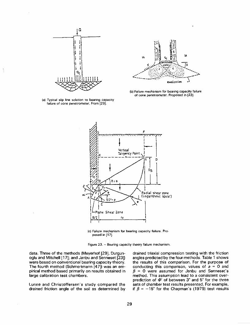
+a
,
1"1'1..,.1'"
.!"till Ii
,'
1
11' !1:
'os11.1
I', 1 ';q\ . 5
IA IWI. ~ ;\:11IA
)II.I:~"I~'II~:UI:\
<$ ~~;.,:~ ~
<~::~~~~;g&4:$gf;::>lc:ealiZQ t ion
(b) Failure mechanism for bearing capacity failure
of cone penetrometer. Proposed in [23].(a) Typical slip line solution to bearing capacity
failure of cone penetrometer. From [29].
F(";'~'
,
~
Redid! S~;;.~ z::>n~
~'(LogCirithmicS?1:41)
>J
(c) Failure mechanism for bearing capacity failure. Pro-posed in [17].
Figure 23. - Bearing capacity theory failure mechanism.
data. Three of the methods (Meyerhof [29], Durgun-oglu and Mitchell [17]; and Janbu and Senneset [23])were based on conventional bearing capacity theory.The fourth method (Schmertmann [47]) was an em-pirical method based primarily on results obtained inlarge calibration test chambers.
drained triaxial compression testing with the frictionangles predicted by the four methods. Table 1 showsthe results of this comparison. For the purpose ofconducting this comparison, values of a = 0 andf3 = 0 were assumed for Janbu and Senneset'smethod. This assumption lead to a consistent over-prediction of (/J' of between 3° and 5° for the threesets of chamber test results presented. For example,if f3 = -15° for the Chapman's (1979) test results
Lunne and Christoffersen's study compared thedrained friction angle of the soil as determined by
29
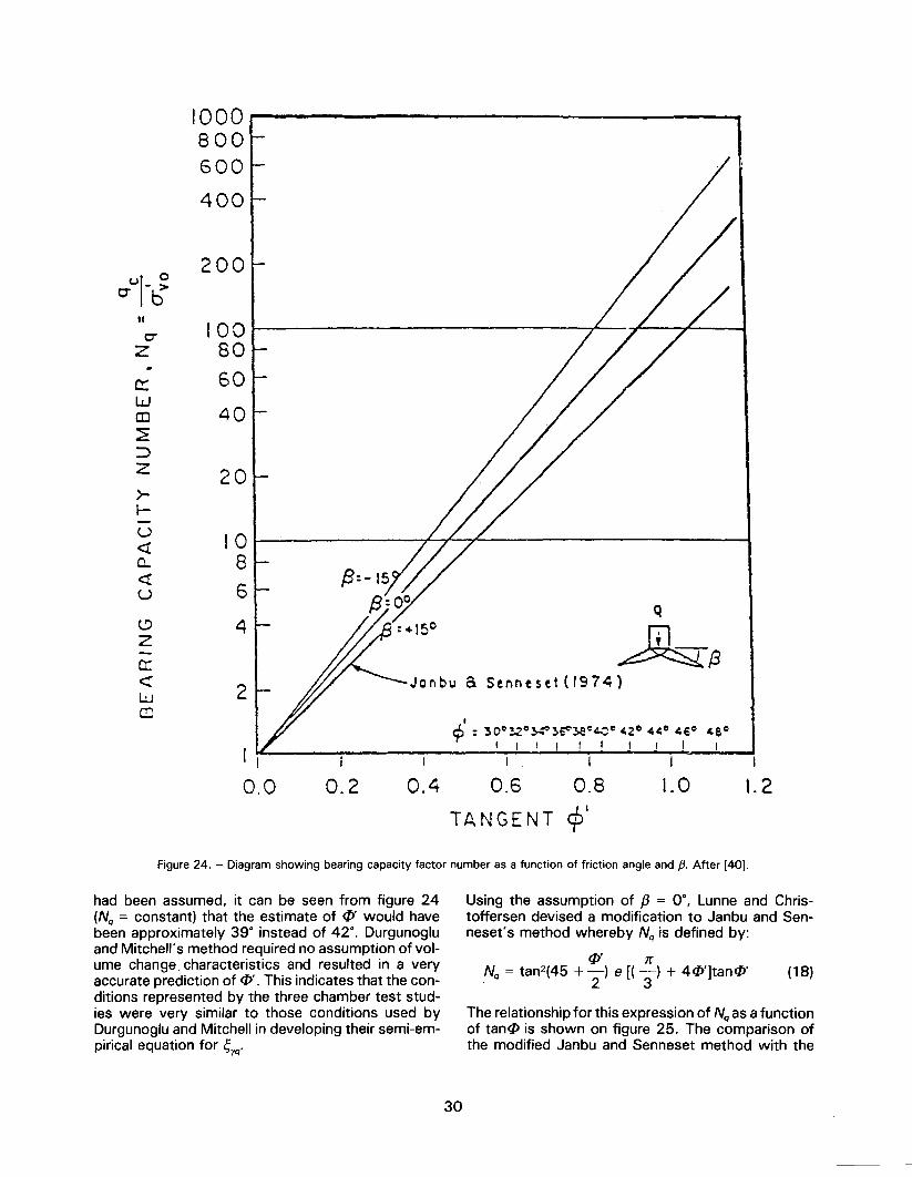
C7UI-~
II
0-Z
a:::wCD~::>z
>-I-U<!:Q..<!:u
t:>Zcr:<wCD
0.4 0.6 0.8
TANGENT cp'
1000800600
400
q
~tBSennese1 (l974)
I
c? : 300~o;}..-e~se->ec~O l,ZC l,l,° 46° 4SoI I I 1 I I ,! I
I I
1.0I
1.2
200
1008060
40
20
1086
4
2
! I
0.0 0.2
Figure 24. - Diagram showing bearing capacity factor number as a function of friction angle and p. After [40].
had been assumed, it can be seen from figure 24(Nq = constant) that the estimate of <P'would havebeen approximately 39° instead of 42°. Durgunogluand Mitchell's method required no assumption of vol-ume change. characteristics and resulted in a veryaccurate prediction of <P'.This indicates that the con-ditions represented by the three chamber test stud-ies were very similar to those conditions used byDurgunoglu and Mitchell in developing their semi-em-pirical equation for ~rq'
Using the assumption of f3 = 0°, Lunne and Chris-toffersen devised a modification to Janbu and Sen-neset's method whereby Nq is defined by:
<P' nNq = tan2(45 + -) e [( -) + 4<P']tan<P'
2 3(18)
The relationship for this expression of Nqas a functionof tan<P is shown on figure 25. The comparison ofthe modified Janbu and Senneset method with the
30
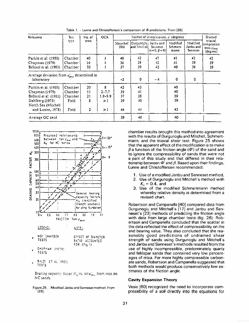
Rtfertnce Tc;: :':0. of OCR ~klhod o~ ir.:trp:~:3tion, .:' (deiTt~~) D:zintdty;:: Itsn triaxial
:-'k).trhor DurfunC'iJu i Ja::~u and \Iodjfi:d ~Iodi~ed ,om~rtnion1961 an~ ~li!d..:lJi Str.new Schrnen- Janbu and ItSU ";".l(z=O, C=O) mann Stnnt~CI (dc.:tt~)
hrkin et aI. (1980) Cha...b~r 40 1 40 42 ~i 41 42 42Cha;:>:nan (1979) Char.1bcr 16 1 36 39 ., ~1 39 39~-Bellotti cl a!. (1983) Ch2:..ber 30 1 37 39 J2 40 39 39,
A \'e~agc deviation (rom .;;.,.. de:erwined ir.
I I IlaboratOry -2 0 -4 0 0
Parkin et aI. (1980) Char:-.'t>er 20 8 42 43 40Chapman (1979) Chamber 11 2-7.7 39 41 40BelJoai et al. (1983) Cha;;: ber 21 1.9-9.9 37 38 39Dahlberg (1975) Fidd 8 >1 39 40 39NO!1~ Sea (Mitchell
I land Lunne. ]978) Field 2 >1 44 44 ! 42
Average OC sar.d 39 4()I I
40I I
Table 1. - Lunne and Christofferson's comparison of <Ppredictions. From [26J.
H\~O
e~o
600>00
~~
% ;CO
Prt~tH: rt!~~ior.shi~btt...ttn t~n~~..lnd,,~ fer HC ~I~:S
~: -IS.
:5200-~<...
£!. C
>- 100
S 6C
~ 60:5 SOc:> 1.0
g 3C<~ 20
IGfntr~l burir'9cl~Hity !ICtt~
;"'c (l:\c:ififC
i;.:-;:'\:tt s:::.:t.on J
,t:..- strl~ !:.-Gct.on
H0.. 05 H t,0~ . , CE 05
F;,I::i::N 1M~.;~..
l~GE"';): N~7: :
. N(il'CHt.~~£~iESTS
U'£Ci 0' DI:"~,ET£;(~;.710 /.::~:.!NTEuFC~ IF.;~)
C!i:";:>~.t." (Hi~~HSiS
6.:...0: n:..~ :';::iHS:S
B~2::::t '2pa::i:'.. :,::0: ?". '"S. :2;-.::~., fro:;,,; [:51s on
1"C sa~cs.'.
"..
Figure25. - Modified Janbu and Senneset method. From[26].
chamber results brought this method into agreementwith the results of Durgunoglu and Mitchell, Schmert-mann, and the triaxial shear test. Figure 25 showsthat the apparent effect of the modification is to make{3a function of the friction angle (cP') of the sand andto ignore the compressibility of sands that were nota part of this study and that differed in their rela-tionship between cP'and {3.Based upon their findings,Lunne and Christoffersen recommended:
1. Use of a modified Janbu and Senne set method,2. Use of Durgunoglu and Mitchell's method with
Ko = 0.4, and3. Use of the modified Schmertmann method
whereby relative density is determined from arevised chart,
Robertson and Campanella [40] compared data tromDurgunoglu and Mitchell's [17] and Janbu and Sen-neset's [23] methods of predicting the friction anglewith data from large chamber tests (fig. 26). Rob-ertson and Campanella concluded that the scatter inthe data reflected the effect of compressibility on theend bearing value. They also concluded that the rea-sonably good predictions of undrained shearstrength of sands using Durgunoglu and Mitchell'sand Janbu and Senneset's methods resulted from theuse of highly incompressible, predominately quartzand feldspar sands that contained very low percent-ages of mica, For more highly compressible carbon-ate sands, Robertson and Campanella suggested thatboth methods would produce conservatively low es-timates of the friction angle.
Cavity Expansion Theory
Vesic [60] recognized the need to incorporate com-pressibility of a soil directly into the equations for
31
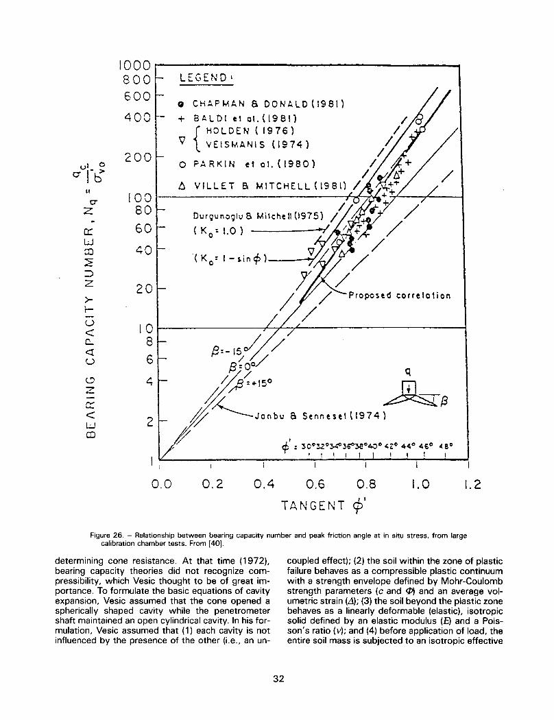
crUI-J
"C7
Z
cr:wOJ:2::>z
>-i-u<!c...
~u0Zc::<UCD
1000800600
400
200
10080
60
40
20
108
6
4
2
LEGENDI
0 CHAPMAN a DONALD(1981)+ BALDI et 01.(1981)
{HOLDEN (1976)
'V VEISMANIS (l974)
0 PARKIN et 01. (1980)
determining cone resistance. At that time (1972),bearing capacity theories did not recognize com-pressibility, which Vesic thought to be of great im-portance. To formulate the basic equations of cavityexpansion, Vesic assumed that the cone opened aspherically shaped cavity while the penetrometershaft maintained an open cylindrical cavity. In his for-mulation, Vesic assumed that (1) each cavity is notinfluenced by the presence of the other (i.e., an un-
I::. VILLET 8 MITCHELL (1981)
/DurQunOQlua Milche II(1975) /(Ko=I.O) ...; I
'(Ko:I-~in~)
/3:-15/ //3{00/
// jf3 =+150
//,y~JOnbU
(f/
I!
0.0 0.2 0.4
correlotion
q
~(3a SenneH1 (1974)
I
~ : ~O~3.2o> c~~c~o ,-,c 4~0 460 «80, I I I I I I 1 1 1
I I I
0.6 0.8 1.0 1.2
TANGENT cp'
Figure26. - Relationship between bearing capacity number and peak friction angle at in situ stress, from largecalibration chamber tests. From [40].
coupled effect); (2) the soil within the zone of plasticfailure behaves as a compressible plastic continuumwith a strength envelope defined by Mohr-Coulombstrength parameters (c and 4» and an average vol-umetric strain (.1); (3) the soil beyond the plastic zonebehaves as a linearly deformable (elastic), isotropicsolid defined by an elastic modulus (E) and a Pois-son's ratio (v); and (4) before application of load, theentire soil mass is subjected to an isotropic effective
32
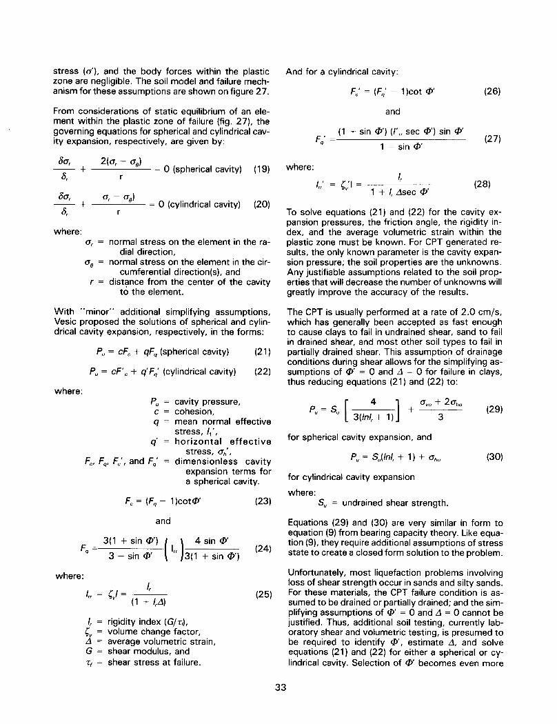
oa, 2(a, - ao)= 0 (sphericalcavity) (19)-+ (j,
(ja, a, - ao)= 0 (cylindrical cavity) (20)-+ (j, r
stress (0'), and the body forces within the plasticzone are negligible. The soil model and failure mech-anism for these assumptions are shown on figure 27.
From considerations of static equilibrium of an ele-ment within the plastic zone of failure (fig. 27), thegoverning equations for spherical and cylindrical cav-ity expansion, respectively, are given by:
where:a, = normal stress on the element in the ra-
dial direction,ao = normal stress on the element in the cir-
cumferential direction(s), andr = distance from the center of the cavity
to the element.
With "minor" additional simplifying assumptions,Vesic proposed the solutions of spherical and cylin-drical cavity expansion, respectively, in the forms:
Pu = cFe + qFq (spherical cavity)
Pu = cF' e + q' Fq' (cylindrical cavity)
(21 )
(22)
where:Pu = cavity pressure,c = cohesion,q = mean normal effective
stress, I,',q' = horizontal effective
stress, ah',Fe, Fq, Fe', and Fq' = dimensionless cavity
expansion terms fora spherical cavity.
Fe = (Fq - 1 )cotCP' (23)
and
3(1 + sin CP')
( )
4 Sin cPFq -
3 - sin CP' I" 3(1+'
sin ~')(24)
where:I,
'"= 'J =
(1 + 1,.1)(25)
"= rigidity index (G/7:,),
'v = volume change factor,.1 = average volumetric strain,G = shear modulus, and7:, = shear stress at failure.
And for a cylindrical cavity:
Fe' = (Fq' - 1 )cot cP' (26)
and
F' =(1 + sin cP') (I'" sec cP') sin cpo
q
1 - sin cPo(27)
where:I,
I' = "I =rr v1 + I, L\sec CP'
(28)
To solve equations (21) and (22) for the cavity ex-pansion pressures, the friction angle, the rigidity in-dex, and the average volumetric strain within theplastic zone must be known. For CPT generated re-sults, the only known parameter is the cavity expan-sion pressure; the soil properties are the unknowns.Any justifiable assumptions related to the soil prop-erties that will decrease the number of unknowns willgreatly improve the accuracy of the results.
The CPT is usually performed at a rate of 2.0 cm/s,which has generally been accepted as fast enoughto cause clays to fail in undrained shear, sand to failin drained shear, and most other soil types to fail inpartially drained shear. This assumption of drainageconditions during shear allows for the simplifying as-sumptions of CP' = 0 and .1 = 0 for failure in clays,thus reducing equations (21) and (22) to:
[4
] avo + 2ahoP=S +u u
3(1nl, + 1) 3(29)
for spherical cavity expansion, and
Pu = Sj/nl, + 1) + aho (30)
for cylindrical cavity expansion
where:Su = undrained shear strength.
Equations (29) and (30) are very similar in form toequation (9) from bearing capacity theory. Like equa-tion (9), they require additional assumptions of stressstate to create a closed form solution to the problem.
Unfortunately, most liquefaction problems involvingloss of shear strength occur in sands and silty sands.For these materials, the CPT failure condition is as-sumed to be drained or partially drained; and the sim-plifying assumptions of cPo= 0 and .1 = 0 cannot bejustified. Thus, additional soil testing, currently lab-oratory shear and volumetric testing, is presumed tobe required to identify cP', estimate .1, and solveequations (21) and (22) for either a spherical or cy-lindrical cavity. Selection of cpobecomes even more
33
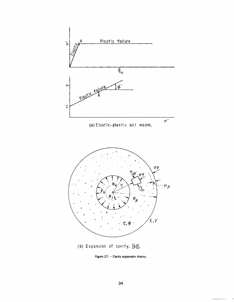
b
Cv
Plastic failure
.....
c
(a)Elastic-plastic soil model.
. ,
c.cp,
(b) Expansion of cavity. [§Q].
Figure 27. - Cavity expansion theory.
34
0-'
}-Lp
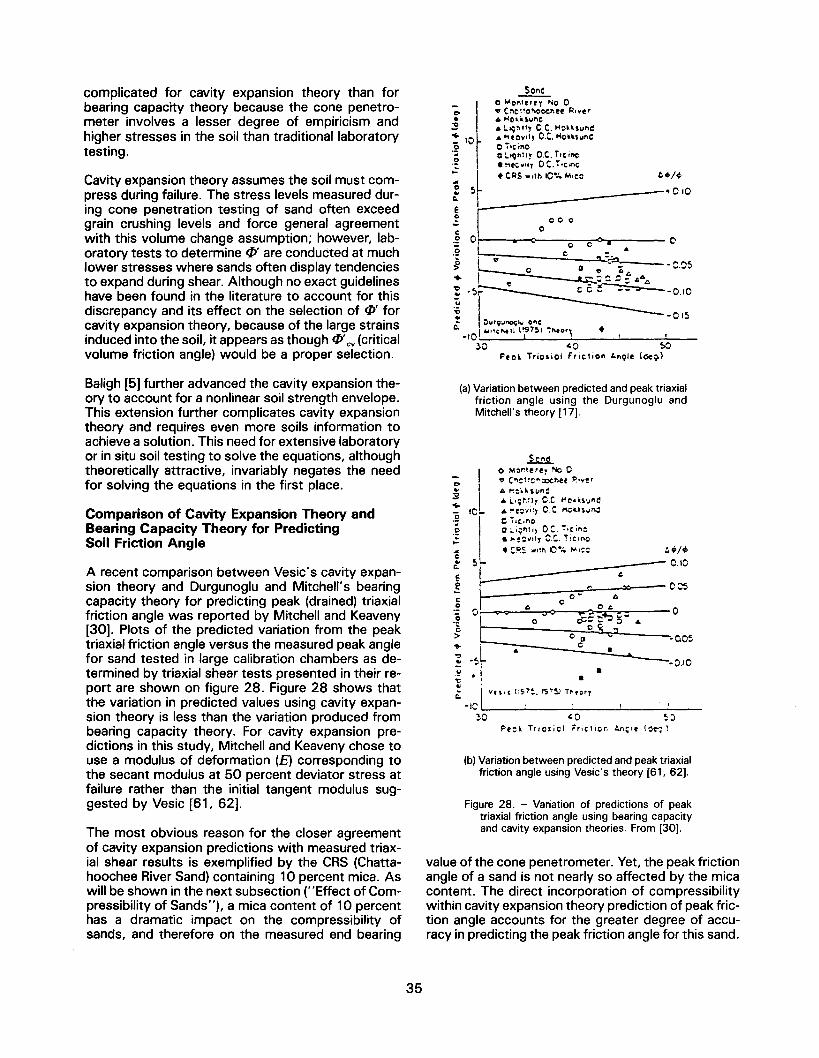
complicated for cavity expansion theory than forbearing capacity theory because the cone penetro-meter involves a lesser degree of empiricism andhigher stresses in the soil than traditional laboratorytesting.
Cavity expansion theory assumes the soil must com-press during failure. The stress levels measured dur-ing cone penetration testing of sand often exceedgrain crushing levels and force general agreementwith this volume change assumption; however, lab-oratory tests to determine CP'are conducted at muchlower stresses where sands often display tendenciesto expand during shear. Although no exact guidelineshave been found in the literature to account for thisdiscrepancy and its effect on the selection of cpoforcavity expansion theory, because of the large strainsinduced into the soil, it appears as though CP'cv (criticalvolume friction angle) would be a proper selection.
Baligh [5] further advanced the cavity expansion the-ory to account for a nonlinear soil strength envelope.This extension further complicates cavity expansiontheory and requires even more soils information toachieve a solution. This need for extensive laboratoryor in situ soil testing to solve the equations, althoughtheoretically attractive, invariably negates the needfor solving the equations in the first place.
Comparison of Cavity Expansion Theory andBearing Capacity Theory for PredictingSoil Friction Angle
A recent comparison between Vesic's cavity expan-sion theory and Durgunoglu and Mitchell's bearingcapacity theory for predicting peak (drained) triaxialfriction angle was reported by Mitchell and Keaveny[30]. Plots of the predicted variation from the peaktriaxial friction angle versus the measured peak anglefor sand tested in large calibration chambers as de-termined by triaxial shear tests presented in their re-port are shown on figure 28. Figure 28 shows thatthe variation in predicted values using cavity expan-sion theory is less than the variation produced frombearing capacity theory. For cavity expansion pre-dictions in this study, Mitchell and Keaveny chose touse a modulus of deformation (E) corresponding tothe secant modulus at 50 percent deviator stress atfailure rather than the initial tangent modulus sug-gested by Vesic [61, 62].
The most obvious reason for the closer agreementof cavity expansion predictions with measured triax-ial shear results is exemplified by the CRS (Chatta-hoochee River Sand) containing 10 percent mica. Aswill be shown in the next subsection ("Effect of Com-pressibility of Sands"), a mica content of 10 percenthas a dramatic impact on the compressibility ofsands, and therefore on the measured end bearing
~
f
C "'on'tlry PlIo 0.. C:'IO'~O"OOQlff R,vrr. ~o'.~~nC:
.
"'
~
~
~~:
'
10
6 "'Q:'Illy O.C. MC..sunC~ 6 "'tov.l) O.C.HO'.sunC
C'riCir\Oat'QMI)' O.C.Tlcinc.~KYI'J OC.T,t,no
~
+ CRS ..11> IC'~ M,CO t.~/~; ~
- .J -+010
i r /00.:.~~. '
~ L C O' - . OO~
I..
".~':':.:;=~.~
: '~
r
'" c c 0--- - --0.10
! -Ol~.. Ou'9..,~I"onec..'01 ""'t"OIi';7:>1~...o" +, .
~O ~ 0 ~Pto. Trio.iOI FriClion lonQlr (oe~)
(a) Variation between predicted and peak triaxialfriction angle using the Durgunoglu andMitchell's theory [17].
~
I
0 MO~'frfJ fib 0
0> v C"~1~:l'\o:xhee ~Iv:r
! ~ ,..~i.kSun~
... 6 ~,;~'IJ O.C Ho..s~nd
- 10:- .. !'Jt~"'I:) C.C. Mc...,,,,n~
~
l; ~:~~~~)0:. ~IC ;nc
~ . "",~~",IJO.~.:icino... . :~5 ...!th().~ ..,,'::t:.. ~
~ -~c'
~ .'u~ I 0 0
o~- C~;: .,,10""":":":1-...
.~ t 0 o=~~ -:>'5
6
; 'L
6
C~ :. -. o.o~
f .~, ~O)O~ .~ . ."'C.
v,\it ':$'~. 'S'.'~ T"'tC'J
-IC
:.~/"
=°,10005
0
~o '0 !;;)Pe:~ TriOJiCI rriC1ior. An~lt (~e--; ~
(b) Variation between predicted and peak triaxialfriction angle using Vesic's theory [61, 62].
Figure 28. - Variation of predictions of peaktriaxial friction angle using bearing capacityand cavityexpansiontheories. From [30].
value of the cone penetrometer. Yet, the peak frictionangle of a sand is not nearly so affected by the micacontent. The direct incorporation of compressibilitywithin cavity expansion theory prediction of peak fric-tion angle accounts for the greater degree of accu-racy in predicting the peak friction angle for this sand.
35
As suggested by Mitchell and Keaveny, accuratelypredicting peak friction angle is important when pre-dicting end bearing pile load capacity. For such pre-dictions, conservative estimates of friction angle forcompressible sands, as generally obtained from the-ories based on bearing capacity, will grossly under-estimate the end bearing capacity of the pile. Thiscomparison suggests that, when an accurate predic-tion of peak friction angle is required for computa-tional purposes, the cavity expansion theory, alongwith the necessity of sampling and additional labo-ratory testing, is justified.
The relationship between the drained friction angle,as determined by the CPT methods, and the un-drained steady-state friction angle (as previously de-scribed in the section "Soil Behavior Model") has notyet been explored. One of the primary aspects of acomplete soil model would be to develop this rela-tionship and thereby deduce the undrained peak andresidual shear strengths of a soil directly from CPTdata.
Effect of Compressibility of Sands
Compressibility of a sand has been mentioned in con-nection with both bearing capacity and cavity ex-pansion theories. It is generally recognized thatincreases in compressibility of a sand lower the endbearing tip resistance. For a clean quartz sand, theprimary causes for a change in compressibility relateto changes in relative density (Le., void ratio) andgrain crushing. For sands in situ, compressibility isalso a function of cementation, stress condition, min-eralogy, and many other factors. For example, Harriset al. [20] have shown that small changes in per-centages of mica, between 0 and 10 percent, canhave significant effects on the initial tangent modulusEo(fig. 29) as well as a secant modulus to 50 percentdeviator stress at failure.
Robertson and Campanella [40] prepared the graphon figure 30 to illustrate the effect of compressibilityon predictions of relative density. Summarized in thisdiagram are methods of predicting relative density(Dr)proposed by Schmertmann [46]; Baldi et al. [4];and Villet and Mitchell [63]. Note the relationshipsbetween curve 3 at Dr = 40 percent and curve 1 atDr = 40 percent and Dr = 80 percent. The dynamicbehavior of a sand at Dr = 80 percent is very differentfrom that at Dr = 40 percent; yet without knowingthe compressibility of the granular structures beingtested, estimates of relative density can easily varyby as much as :t 20 percent from the mean. Fromthe standpoint of mica content, this could mean thata change of only a few percentage points between0 and 10 percent could change the predicted behav-ior significantly.
CONE PENETRATION PRACTICE
Introduction
The lack of a good theoretical soil model and an ac-curate analytical technique to link CPT data to un-drained shear strength of potentially liquefiable soilshas led engineers to seek empirical relationships fordesign and analysis in earthquake prone areas. Bydeveloping empirical CPT models, engineers hope toseparate soils exhibiting stable or safe behavior fromthose that are unstable or potentially unsafe. TheCPT data are often used for locating and focusingattention on the specific zones of soil whose behavioris questionable. Once such a zone has been locatedand fully delineated by the CPT, other in situ tests,such as the standard penetration test or samplingand laboratory testing, verify the CPT results andprovide more detailed design information.
Although theory may not fully substantiate the CPT-soil empirical relationships, these relationshipsshould be based on a logical set of first-order, soil-test condition, influencing factors. If these factors arenot fully understood, the limitations on the validity ofthe empirical correlations are unknown. Thus, the va-lidity of empirical correlations developed in one lo-cation for one soil under one set of boundaryconditions is unknown for use in another locationwhere soil or boundary conditions are different.Therefore, a complete empirical relationship shouldpresent methods for evaluating the changes in theinfluencing factors as well as provide guidelines fordesign. For this reason, this section not only presentsthe CPT empirical relationships currently used for es-timating the liquefaction susceptibility of soils, butalso attempts to define the factors that may haveinfluenced the development of those relationships.
Influencing Factors of the CPT
The factors that influence measured CPT values maybe placed in three categories: first, factors resultingfrom penetrometer design and geometry; second,factors related to soil properties; and third, factorsrelated to the stress field in the soil caused by thepenetration of the tool. The latter is the soil-structureinteraction factor.
Robertson and Campanella [41] pointed out the ef-fects of machine tolerances on individual penetro-meter elements, the effects of temperature onelectronic components, and the effects of unequalsurface areas of cone tip and sleeve components.Levadoux and Baligh [24] investigated the effects ofchanging the cone apex angle for penetration in clays.Lunne et al. [27] presented further methods for eval-uating the effects of thermal shift, load cell range,and other factors related to penetrometer design.
36
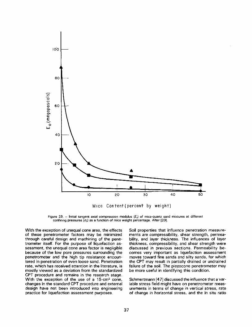
(i)
0uen
6000.00'>Q)
E
0W
40
10.0
80
20
10 20 30 40 50
Mica Content{percent by weight)
Figure 29. - Initial tangent axial compression modulus (Eo) of mica-quartz sand mixtures at differentconfining pressures (0"3)as a function of mica weight percentage. After [20].
With the exception of unequal cone area, the effectsof these penetrometer factors may be minimizedthrough careful design and machining of the pene-trometer itself. For the purpose of liquefaction as-sessment, the unequal cone area factor is negligiblebecause of the low pore pressures surrounding thepenetrometer and the high tip resistance encoun-tered in penetration of even loose sand. Penetrationrate, which has received attention in the literature, ismostly viewed as a deviation from the standardizedCPT procedure and remains in the research stage.With the exception of the use of a 15-cm2 cone,changes in the standard CPT procedure and externaldesign have not been introduced into engineeringpractice for liquefaction assessment purposes.
Soil properties that influence penetration measure-ments are compressibility, shear strength, permea-bility, and layer thickness. The influences of layerthickness, compressibility, and shear strength werediscussed in previous sections. Permeability be-comes very important as liquefaction assessmentmoves toward fine sands and silty sands, for whichthe CPT may result in partially drained or undrainedfailure of the soil. The piezocone penetrometer maybe more useful in identifying this condition.
Schmertmann [47] discussed the influence that a var-iable stress field might have on penetrometer meas-urements in terms of change in vertical stress, rateof change in horizontal stress, and the in situ ratio
37

0- >I::)
V)
\-0
.J:J
U)(f)
wc::I-en-.J<::uI-0::W>W>I-UWL:..lJ...W
CONE RESISTANCE, Qc' bars
0 200 300 400 500100a
2
3
4
5
Dr: 80%
CD SCHMERTMANN (1976) Hilton Mines Sond - HiQh Compressibility
(f) BALDI et ol.(1982) Ticino Send - MoGerate Compressibility
CID VILLET 8 MITCHELL (1981) Monterey Sand -Lo.. Compressibility
Figure 30. - Comparison of different relative density relationships. From [40].
of horizontal to effective vertical stresses (Ko).Thegeneral trend is for cone resistance to increase withan increase in mean normal effective stress. The rateof increase in tip resistance is not expected to belinear with changes in effective stress condition, justas soil properties such as compressibility and shearstrength are neither linearly related to nor constantwith changes in void ratio associated with changesin stress condition.
CPT-SPT Correlations
The SPT (standard penetration test) has been usedextensively for liquefaction assessment in the United
States, Japan, China, and other countries. To makeuse of this extensive SPT data base, many investi-gators have tried to develop relationships betweenCPT and SPT results. The early conversion attemptswere made to determine a constant for the ratio ofcone tip resistance to SPT blow count (qc/N). Rob-ertson et al. [43] noted that many of the differentqc/Nratios reported in the literature had some degreeof correlation with mean grain size (D50)of a sandand developed the chart shown on figure 31. Seedand De Alba [53] updated this curve with new dataand presented the graph shown on figure 32. How-ever, Farrar [18] found a great deal of scatter in thecorrelation with D50when applied to a variety of sitesin Japan, as shown on figure 33.
38
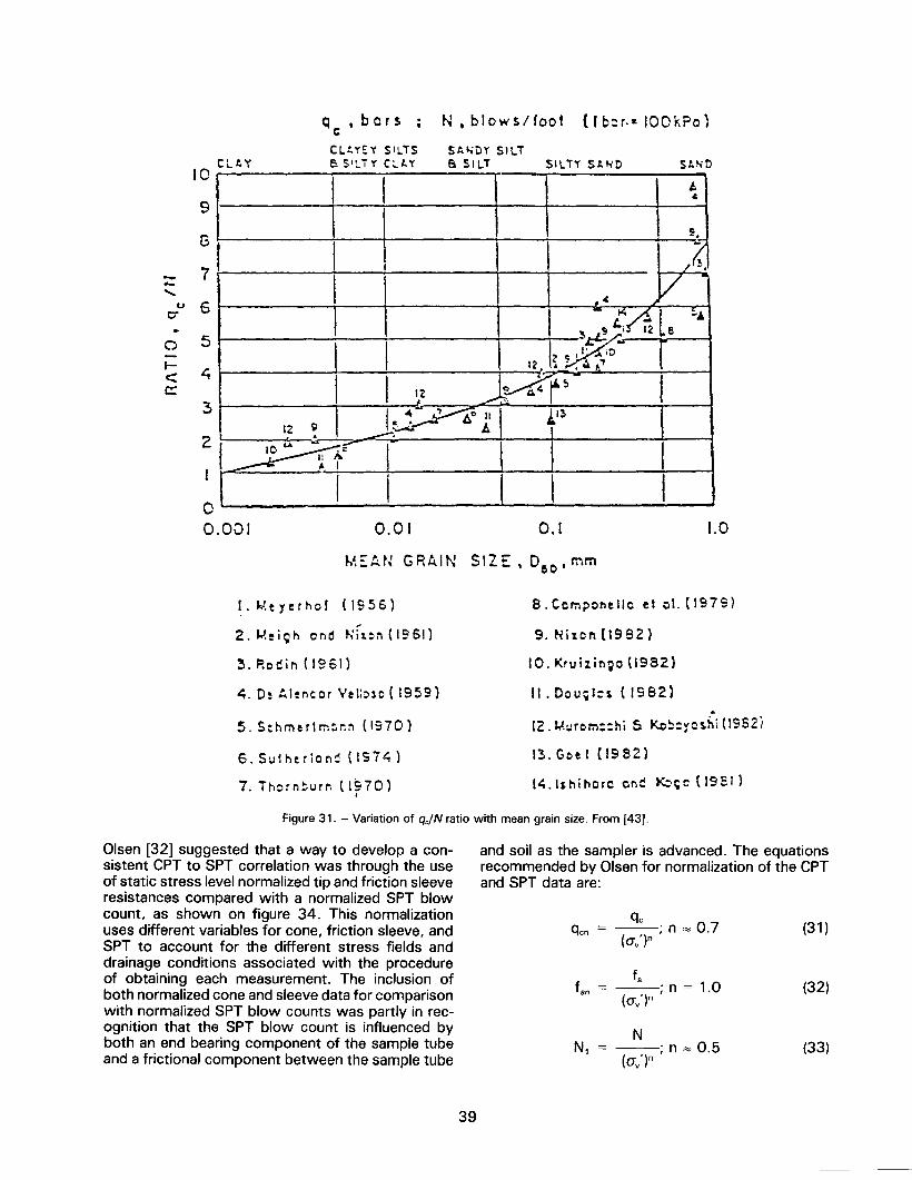
CLt.y10
9
q ,bars ic
CL:.yEY SILTSB SI!..TY CLt.y
N.blows/foot (I bop JOOkPo)
St.,,!)y SILTe. SILT SILTY SLt-ID SLND
t~
0
r-<C!:
5
4
...
81
- 7--.....
u 6C"
3
00.001
I
0.01 0.1 1.0
M :: to.N G RA INS 1Z E , D60 '
mm
I. W.eyerner (IS56)
2. J),ei~h end "";:'01'1(1961)
B.Componellc et 01. (1979)
9. Nixen{t992)
:3. Ro~in (1961)
~. De t..lencor Vel:::>se(1959)
10. Kru i I i n ~ e (J 9 B 2)
II. Dou;l:s (19B2)
5. S:hmerlm:.r:n (1970)
6.Sulherjon~ (1974)
.12 .lJ.urom::hi 5. Kr;~:rO\hi (1962i
7. inorr,~urn (1970)I
1:3. Goe I (198Z)
14.lshiherc ond ~~c (19EI)
Figure 31. - Variation of qjNratio with mean grain size. From [43].
Olsen [32] suggested that a way to develop a con-sistent CPT to SPT correlation was through the useof static stress level normalized tip and friction sleeveresistances compared with a normalized SPT blowcount, as shown on figure 34. This normalizationuses different variables for cone, friction sleeve, andSPT to account for the different stress fields anddrainage conditions associated with the procedureof obtaining each measurement. The inclusion ofboth normalized cone and sleeve data for comparisonwith normalized SPT blow counts was partly in rec-ognition that the SPT blow count is influenced byboth an end bearing component of the sample tubeand a frictional component between the sample tube
and soil as the sampler is advanced. The equationsrecommended by Olsen for normalization of the CPTand SPT data are:
qcqcn = -; n ~ 0.7
(av')n(31 )
fsfsn = -;n = 1.0
(av')n(32)
NN, = -;n~0.5
(av')n(33)
39
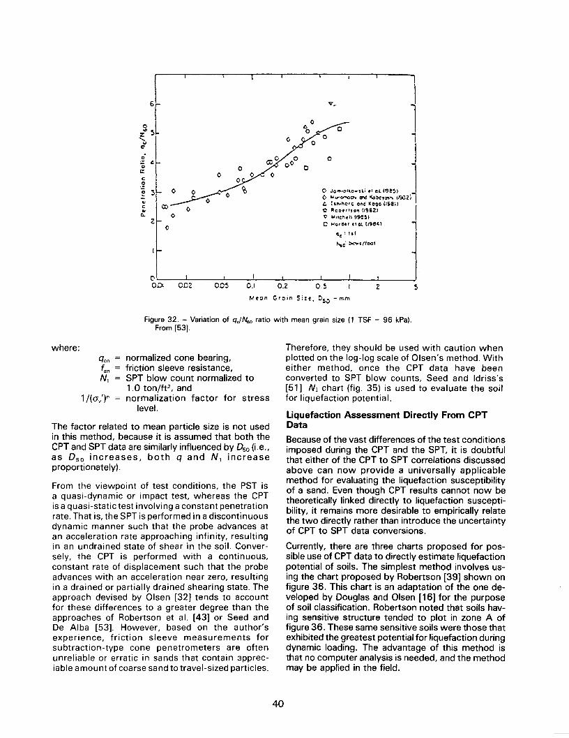
.I
%~J.......
'"co
c'.= .;c 0c::
0c:c
~3 0
..c: I:::> 0"co. 0
Z0
JI
I
0 ".,,, ,.. 0"""l
0""""""'''''
cr<:I(cx,,,,.. Ir,.:;,;1~ :,...ihc,c onc kCQC{IS!i),::. ReD"IIO" 1198"
I~ ""1thtll tr9!~)
0 Mo,dl'r tl 0:.. l198C\ '~c : tlf
","c' ~II/OO'
v.
c-0.01
I
0.1
Meon Groin Size. DSu -",.m
002 005
0
0.2 05 z 5
Figure 32. - Variation of qc!N6oratio with mean grain size (1 TSF = 96 kPa).From [53].
where:qcn = normalized cone bearing,fsn = friction sleeve resistance,N, = SPT blow count normalized to
1.0 ton/ft2, and1/(av')n = normalization factor for stress
level.
The factor related to mean particle size is not usedin this method, because it is assumed that both theCPTandSPTdata are similarlyinfluencedby 050 (i.e.,as 050 increases, both q and N, increaseproportionately) .
From the viewpoint of test conditions, the PST isa quasi-dynamic or impact test, whereas the CPTis a quasi-static test involving a constant penetrationrate. That is, the SPT is performed in a discontinuousdynamic manner such that the probe advances atan acceleration rate approaching infinity, resultingin an undrained state of shear in the soil. Conver-sely, the CPT is performed with a continuous,constant rate of displacement such that the probeadvances with an acceleration near zero, resultingin a drained or partially drained shearing state. Theapproach devised by Olsen [32] tends to accountfor these differences to a greater degree than theapproaches of Robertson et al. [43] or Seed andDe Alba [53]. However, based on the author'sexperience, friction sleeve measurements forsubtraction-type cone penetrometers are oftenunreliable or erratic in sands that contain apprec-iable amount of coarse sand to travel-sized particles.
Therefore, they should be used with caution whenplotted on the log-log scale of Olsen's method. Witheither method, once the CPT data have beenconverted to SPT blow counts, Seed and Idriss's[51] N1 chart (fig. 35) is used to evaluate the soilfor liquefaction potential.
Liquefaction Assessment Directly From CPTData
Because of the vast differences of the test conditionsimposed during the CPT and the SPT, it is doubtfulthat either of the CPT to SPT correlations discussedabove can now provide a universally applicablemethod for evaluating the liquefaction susceptibilityof a sand. Even though CPT results cannot now betheoretically linked directly to liquefaction suscepti-bility, it remains more desirable to empirically relatethe two directly rather than introduce the uncertaintyof CPT to SPT data conversions.
Currently,there are three charts proposed for pos-sible use of CPT data to directly estimate liquefactionpotential of soils. The simplest method involves us-ing the chart proposed by Robertson [39] shown onfigure 36. This chart is an adaptation of the one de-veloped by Douglas and Olsen [16] for the purposeof soil classification. Robertson noted that soils hav-ing sensitive structure tended to plot in zone A offigure 36. These same sensitive soils were those thatexhibited the greatest potential for liquefaction duringdynamic loading. The advantage of this method isthat no computer analysis is needed, and the methodmay be applied in the field.
40
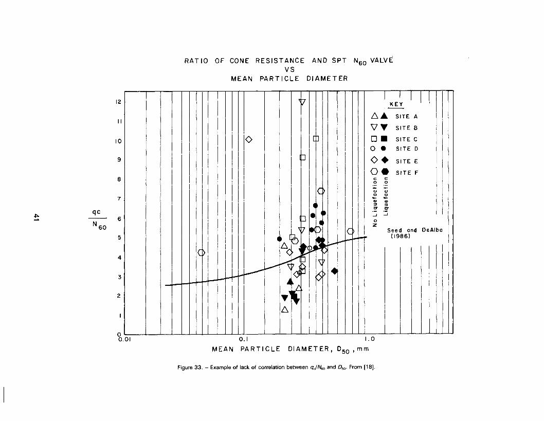
12
II
10
9
8
7
~qc..... - 6
N60
5
4
3
2
'] IKE~
11I
I.-6. SITE A
\1'" SITE B
0 leD I o. SITE CI 0 8 SITE 0I
] I
I
I o. SITE E
I
o. SITE FI I c: c:
0 0I
leT> - -u <.>
I
c c.... ....
4 I 41 41::J ::J
I .~.~I :J8 . ...J ...J
I
bI I c
I ~7~z I
Ie Seed and DeAlba
I4 ~.~j.....oi- ~- (1986)
I6(
....
Ie>I ..-1
~~f.)
~~1\f1
~(Il.--- ~~4i- ~~IbI~~I, I
I~I
6
I
RATIO OF CONE RESISTANCE AND SPT N60 VALVE
VS
MEAN PART I CLE DI AME T ER
00.01 0.1 I. 0
MEAN PARTICLE DIAMETER, D50' mm
Figure 33. - Example of lack of correlation between qc/N.o and 050. From [18].
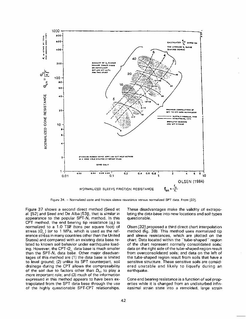
1000.- 600.::c. ~5000. c.. .. -=
: ~OO.~....-- c~.:200
Ul~C"~
100IIc 60U
C" 50
20
10
8
G
4
2
5I 4
40 ~'~~~,J /~~,<:-~~~~,~>:,,~ I 3
.v ,. Of''. "8ar. ~~:'~:~ %"'~~'~: /oc Jo-t'. 810&.10 ~'._:-."":..{.~ :-~...:;.?:.
::"". /OtfIIIO.."'UUD .~~~~~~"':':~'-":...:"'yc.T..~8" OAT" ~ ~~~':'~\x'
"'~'. .-:000 not
n"," 20 "'"~~:\,~~\;.\".--L ~~
;j~'!I":,/!.;x',,~'~~' ,1.~~40I, :~/.i)~,l,;~:1;,-,
.~:~~-~~.~::,~~.'
1/;,'/!r.
1.
'/I//Yf!':
m:"
,j'S'-4~'"'"'-.":,..',1.,1- 1,/1.;1..."
"-10 ~,'I.i.~/)~.'J.'/,.. ...~/ ''X'.i:; !,!!,:'~S,°'l: :00
~~\ // \;!~';(1~'I!':~:,,~~-.~ y
'" "Zi.', I
'::';""~~\':)o"..~-t " 1,//./.,""":.-"":"'v:..,~.' . - "',J' 10
5 /'''' ,'.:\.,~.,"V' ......./ ,~:-."j.".., ~
'",.
~., ~,,:,'$f", :.~ IS-",-. ", / ..,..~,~"..
.'//' ./:':"' \', u."~, ";"~.'",~ ..',,','r;,. "1' '. ',(
"'"-12
":;.;~::~.:.:'>(, \.":~~'~'~:
/ .'/1'./":" ,::,-.; \ ",~' '0, ,..., ., ...-
i \
" ";-'/ ;,;;..//;~, H
~J',:;'::~:::::~\~i/~~ '..i~'t~"t/t;
' ".:"...1:"'I
wt)Z<f0-CI)(.?wa:
.CI~
CAlCUL"'Tt:D k;' .""(.0 CHITw[ .&,,[a...o£ tt.. 'U.IiliQ(CIHAOUI ZONla.
40
wz0t)
0W~...J
<:::E
c:0z
Mr.tOva C'04l..'tUTtO«l Of'
"'YTO C.1 ..011 -callu.u.zc.DI
"Uf"ll'~a.."...-- aCtte.""""'",.,.8cI.#1,.A."'O ""..........( arT . ."UIC.
SAIitD ONL.Y
nUifCU,1iCI""'1. ""'"a "oPt ..c C-AT "«0 _''-''00
. .. .0.. ..~ C-U.TIO""'CI'TOI'......
1 I
0.010.02 0.0. O.Ot C.OI
0.10.2 0.4 0.6 0.8
14 6 8
10
OLSEN (1984)
fSO: ~~
2
NORMALIZED SLEEV~ FRICTION RESISTANCE
Figure 34. - Normalized cone and friction sleeve resistance versus normalized SPT data. From [32].
Figure 37 shows a second direct method (Seed etal. [52] and Seed and De Alba [53]), that is similar inappearance to the popular SPT-N, method. In thisCPT method, the end bearing tip resistance (qcl isnormalized to a 1.0 TSF (tons per square foot) ofstress (Qc ) (or to 1 MPa, which is used as the ref-erence stress in many countries other than the UnitedStates) and compared with an existing data base re-lated to known soil behavior under earthquake load-ing. However, the CPT-Qc data base is much smallerthan the SPT-N, data base. Other major disadvan-tages of this method are (1) the data base is limitedto level ground; (2) unlike its SPT counterpart, soildrainage during the CPT allows the compressibilityof the soil due to factors other than 050 to playamore important role; and (3) much of the informationexpressed in this method appears to have been ex-trapolated from the SPT data base through the useof the highly questionable SPT-CPT relationships.
These disadvantages make the validity of extrapo-lating the data base into new locations and soil typesquestionable.
Olsen [32] proposed a third direct chart interpolationmethod (fig. 38), This method uses normalized tipand sleeve resistances, which are plotted on thechart. Data located within the "tube-shaped" regionof the chart represent normally consolidated soils;data on the right side of the tube-shaped region resultfrom overconsolidated soils; and data on the left ofthe tube-shaped region result from soils that have asensitive structure, These sensitive soils are consid-ered unstable and likely to liquefy during anearthquake.
Cone end bearing resistance is a function of soil prop-erties while it is changed from an undisturbed infin-itesimal strain state into a remolded, large strain
42
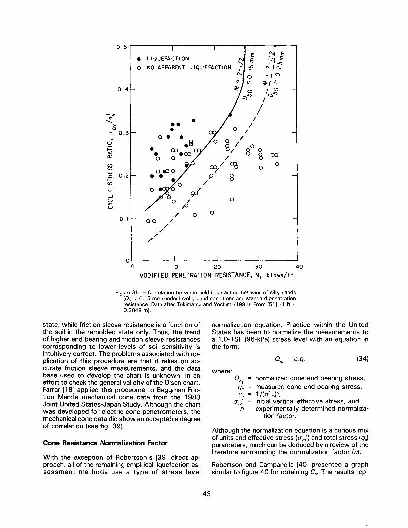
C\Jf E:::::-, E, II')
"/rv
III C
~/!I
I CQII')
/I
//
0/
I
0 I
8 I8
00
II 8 00
<:X7/ ao 00
/9 8
~0 6I
/ 0/
.//
/./
O. 5
. LIQUEFACTION ~ ~0 NO APPARENT LIQUEFACTION -; Jr)
r-..CV
0.4
- >0.......
>0... 0.3
...0 .-0
l-e:[a::
. .0
(f)(f)
~ 0.2I-(f)
U
-J~U
0.1 00
.
0
0
00 10 20 30 40
MODIFIED PENETRATION RESISTANCE. N1 t>lows/ff
Figure 35. - Correlation between field liquefaction behavior of silty sands(050 < 0.15 mm) under level ground conditions and standard penetrationresistance. Data after Tokimatsu and Yoshimi (1981). From [51]. (1 ft =0.3048 mI.
state; while friction sleeve resistance is a function ofthe soil in the remolded state only. Thus, the trendof higher end bearing and friction sleeve resistancescorresponding to lower levels of soil sensitivity isintuitively correct. The problems associated with ap-plication of this procedure are that it relies on ac-curate friction sleeve measurements, and the database used to develop the chart is unknown. In aneffort to check the general validity of the Olsen chart,Farrar [18] applied this procedure to Beggman Fric-tion Mantle mechanical cone data from the 1983Joint United States-Japan Study. Although the chartwas developed for electric cone penetrometers, themechanical cone data did show an acceptable degreeof correlation (see fig. 39).
Cone Resistance Normalization Factor
With the exception of Robertson's [39] direct ap-proach, all of the remaining empirical liquefaction as-sessment methods use a type of stress level
normalization equation. Practice within the UnitedStates has been to normalize the measurements toa 1.0-TSF (96-kPa) stress level with an equation inthe form:
Qc = cnqc1
(34)
where:Qc = normalized cone end bearing stress,
1qc = measured cone end bearing stress,Cn = 1j(a'vo)n,
avo' = initial vertical effective stress, andn = experimentally determined normaliza-
tion factor.
Although the normalization equation is a curious mixof units and effective stress (avo') and total stress (qJparameters, much can be deduced by a review of theliterature surrounding the normalization factor (n).
Robertson and Campanella [40] presented a graphsimi lar to figure 40 for obtaining Cn- The results rep-
43
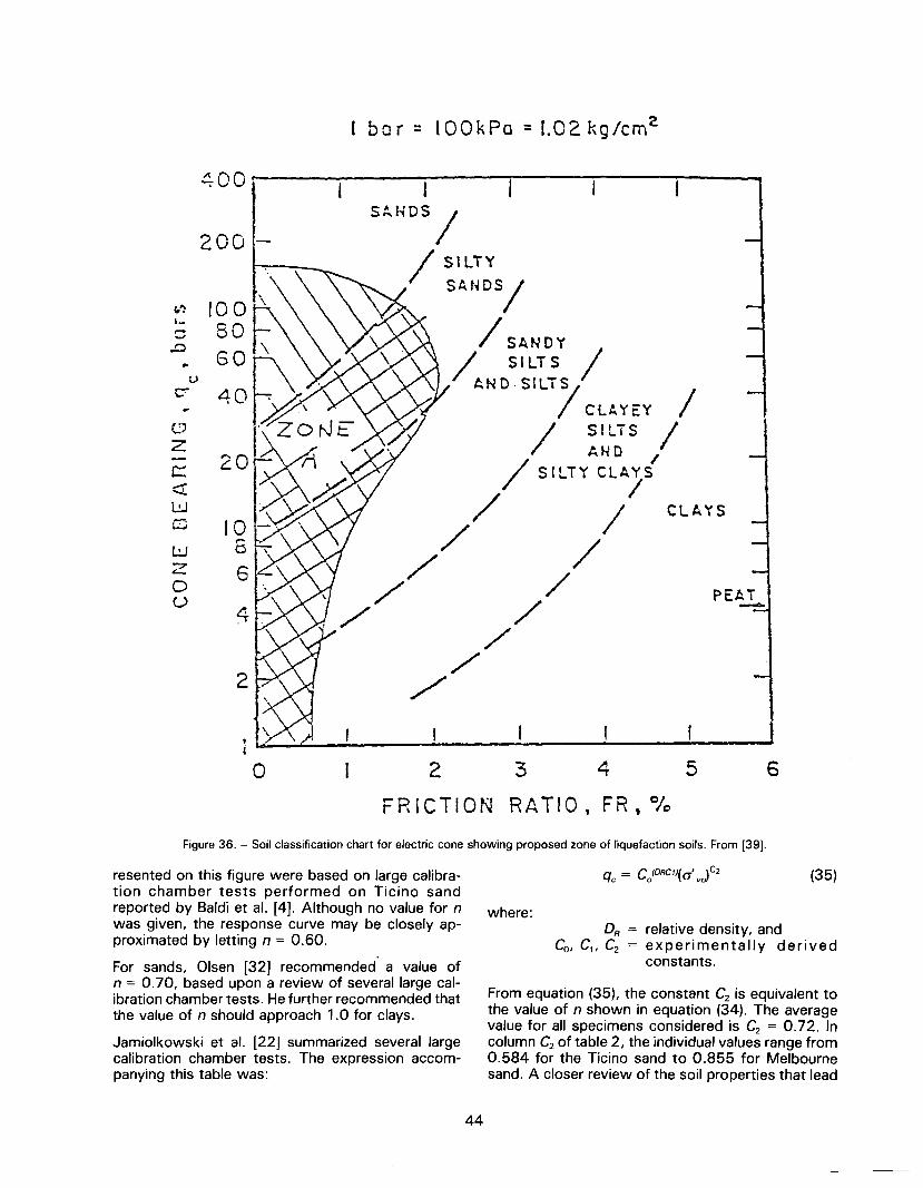
c.")1-,....--
..0
~~c::-
c..:'z-c::::::!WCJ
~z6
0()
4
( bar = 100kPa = 1.02 kg/cmz
ISAHDS
// SILTY
SANDS/
/ SANDY
/ SILTS /AND. S I LT
IS
/CLAYEY
/ SILTS /AND /
/ SILTY CLAYS
/ II
CLAYS
// /
/ //' /
//
/
400
200 -
2
0 2
FRICTION
I
3 4
RAT I0, FR t%
,
5 6
Figure 36. - Soil classification chart for electric cone showing proposed zone of liquefaction soils. From [39].
resented on this figure were based on large calibra-tion chamber tests performed on Ticino sandreported by Baldi et al. [4]. Although no value for nwas given, the response curve may be closely ap-proximated by letting n = 0.60.
For sands, Olsen [32] recommended a value ofn = 0.70, based upon a review of several large cal-ibration chamber tests. He further recommended thatthe value of n should approach 1.0 for clays.
Jamiolkowski et a!. [22] summarized several largecalibration chamber tests. The expression accom-panying this table was:
qc = C/DRC1)(a'vo)C2
where:
(35)
DR = relative density, andCo, C" C2 = experimentally derived
constants.
From equation (35), the constant C2 is equivalent tothe value of n shown in equation (34). The averagevalue for all specimens considered is C2 = 0.72. Incolumn C2of table 2, the individual values range from0.584 for the Ticino sand to 0.855 for Melbournesand. A closer review of the soil properties that lead
44
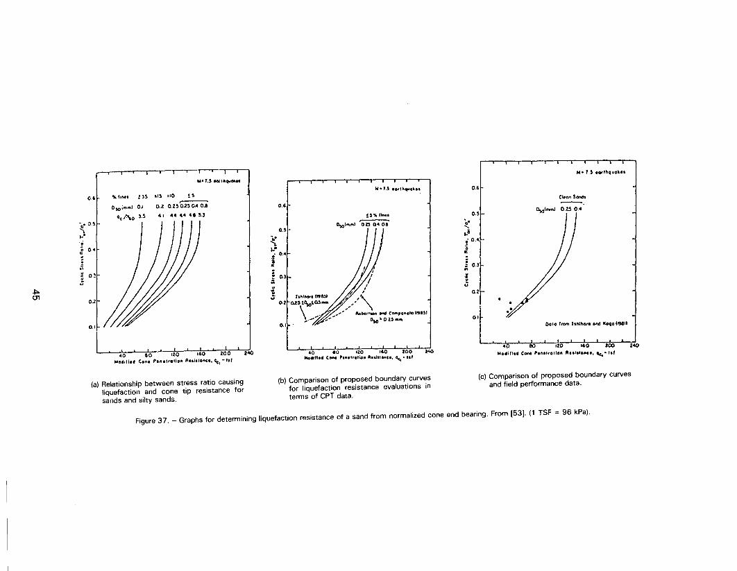
~01
w. 7.~Mel".,...
06 %. fl1\41 ! ]~ 1;1" :10 !. 5,----..
O~;",..I OJ 0.2 0.2~02~C"0.8
~c1\0 ).~ A. A.A"" 48 ~.)
'bO ~.~-...
...",tj
: a".",;;
! O!
0.2
0.'
<0 80 120 160 200WO..UI' Con. "."..,a,I." A..i.lot\u. c:.c.-h'
(a) Relationship between stress ratio causingliquefaction and cone tip resistance forsands and silty sands.
N- '.S lorlhq".h.
0.6
1S"," 11"-1
0.5
~...'. 0.4i.
b"....&...
! 0.<0.~ 0)..
~u
z<o
,.. 7,S .orlhQuo\"
0.6Cloon SoncII
-----O.~ ~IIIYI\) O~O.A
~I I
,I
. /,. I
hhi (t91U1 .~
\'0.2 02' !~("'fNft ':,..."
\ , , """"10ft C ,on" 51,'" D~~O.l"'"''
; Q),;;
..
'"..~...
D.'
2<0 <0 8<> '20 160 zeDMo""8411COAt , ".,&0..
",-',to"u. Ctc...
"'
02
(b) Comparison of proposed boundary curvesfor liquefaction resistance evaluations interms of CPT data.
01
0010 III""hlllhOlO 0,", 11040119811
< eo .20 160 200
MOdifl" Cone ",,",otlOft ".,ilfOftCI. tc... h'
240
(c) Comparison of proposed boundary curvesand field performance data.
Figure 37. - Graphs for determining liquefaction resistance of a sand from normalized cone end bearing. From [53]. (1 TSF =96 kPa).
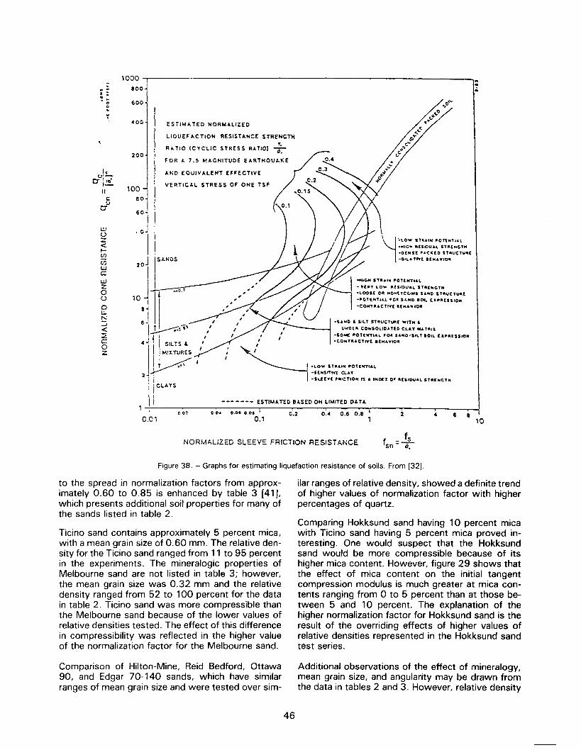
1000~~aoo. :0- ;; 600
~~~OO
ol~C"
I,,,.I-I!
c'-'C"
.'AwD A $oILT ST"UCT~t WITH &uloIet." COHSOLICATtD ClA." IUT"11.
I -SOME ~OT[NTI""L '0. $UIO'S'",' IOU. [1"'U5SIONI .c.Ofrl('''ACTrvt. 8bcAV,O"
~'
-L.OW1'''''''1i(
POTUf'TIAL
-5£H$"'\'( (:.AT"'SU(v( '1III1:nON,S .. '''DEI 0" "[SIDV"L ST"[NCT"
ESTIMJ.TED NORMALIZED
LIOUEFACTION RESISTANCE STRENGTHT.
RJ. TlO (CYCLIC STRESS RATIO)'7i:"
fOR I. 7.5 MAGNITUDE EARTHOUAKE200
100
eo
AND EOUIVJ.LENT EFFECTIVE
VERTICJ.L STRESS Of ONE TSF
L:JUZ<~C/)t;;L:Jc::WZ0U0L:.;N:J<~c:0z
601
.011
20JSJ.NOS
I
>0.l'
..0'
6 - I
I
J...+---;:="~I
~
1
'I' ISIL~: &
,/IMiXTURES
I
11 ~J;.-- .'\I
2
1
1
I
CLio.YS
1I. co:
0.01
..
!
~~lOw sT ,., POTt.nu..\."'-U(;'" "(SOU"'''' STtt[frljCTN-O[HSf '.&.CltE.O S'.UCTUIIIo(
-0'L4 TfVl I[M4W'01lt
rR ., OOT[IIT'AL.. ¥fllll" LO- ,,(S'::)U4I,L
S'''[NCT"-"'OOsIE.
°"~OH( fCCI...
''''HOSTAUCTu..r:
.'"CTt"""U.!,. FC.S""'O
.~ EIII'IUSSIO'C.CON'T"ACTIV[ 'f.M"~ .0.
EST1MJ.TED BJ.SED ON LIMITED DJ.TA
c.o< 0.00 0.00 C.2 O.~ 0.6 o:a I
0.1 , 2 4 6 810
NORMALIZED SLEEVE FRICTION RESISTANCE f - fssn-T
Figure 38. - Graphs for estimating liquefaction resistance of soils. From [32].
to the spread in normalization factors from approx-imately 0.60 to 0.85 is enhanced by table 3 [41 j,which presents additional soil properties for many ofthe sands listed in table 2.
Ticino sand contains approximately 5 percent mica,with a mean grain size of 0.60 mm. The relative den-sity for the Ticino sand ranged from 11 to 95 percentin the experiments. The mineralogic properties ofMelbourne sand are not listed in table 3; however,the mean grain size was 0.32 mm and the relativedensity ranged from 52 to 100 percent for the datain table 2. Ticino sand was more compressible thanthe Melbourne sand because of the lower values ofrelative densities tested. The effect of this differencein compressibility was reflected in the higher valueof the normalization factor for the Melbourne sand.
Comparison of Hilton-Mine, Reid Bedford, Ottawa90, and Edgar 70-140 sands, which have similarranges of mean grain size and were tested over sim-
ilar ranges of relative density, showed a definite trendof higher values of normalization factor with higherpercentages of quartz.
Comparing Hokksund sand having 10 percent micawith Ticino sand having 5 percent mica proved in-teresting. One would suspect that the Hokksundsand would be more compressible because of itshigher mica content. However, figure 29 shows thatthe effect of mica content on the initial tangentcompression modulus is much greater at mica con-tents ranging from 0 to 5 percent than at those be-tween 5 and 10 percent. The explanation of thehigher normalization factor for Hokksund sand is theresult of the overriding effects of higher values ofrelative densities represented in the Hokksund sandtest series.
Additional observations of the effect of mineralogy,mean grain size, and angularity may be drawn fromthe data in tables 2 and 3. However, relative density
46
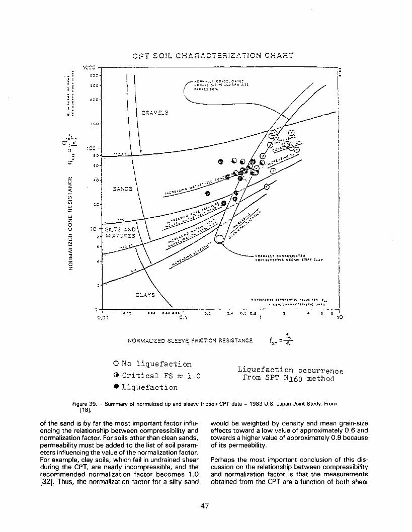
.or""'''',h..........
. !~~I :. ; .""-..,. , -:C.! .".
-~~
'.-.:.,,;'--:-... '.!-II :C:::
~~-.0
C~T S O!L C:-L~R:'CT=:;jZ~ TION C:-iAfiT
~.,
~? .~
r :~=~"t.~;;~~.~,:~.~,;:~(;,::( '...C.(!: J;t,-
~,.
(I
..-:-.,,=.~'..;..'"'\,.."---
',' iouz<
-,..0U
'"..e
~c, ,
:--I
<::E
C<:
"'C"IJ"I..;''!'' ::"'SC\,.I:"'~I;:)"'O..-S£"'S'~IV!. ",(:~.Jw IT:'" ::'.t."
,. "..."n", In IIT&\. ,. ".. ',.. 'IG~"c c.!,.c.',c ;"1."
. I=.:: 0.04 0.: I .:..;1
j
O~,C.: '.' C.$ :.2 2 4 a I
'00.01
NO;::;MAUZ:J SL~=v'~f:=:IC7:CN R:;SISTANC; f =~S~ fr.
ON a liquefaction
~ Critical FS ~ 1.0. Liquefaction
Liquefaction occurrencefrom SPT N160 method
Figure 39. - Summary of normalized tip and sleeve friction CPT data - 1983 U.S.-Japan Joint Study. From[18].
of the sand is by far the most important factor influ-encing the relationship between compressibility andnormalization factor. For soils other than clean sands,permeability must be added to the list of soil param-eters influencing the value of the normalization factor.For example, clay soils, which fail in undrained shearduring the CPT, are nearly incompressible, and therecommended normalization factor becomes 1.0[32], Thus, the normalization factor for a silty sand
would be weighted by density and mean grain-sizeeffects toward a low value of approximately 0.6 andtowards a higher value of approximately 0.9 becauseof its permeability.
Perhaps the most important conclusion of this dis-cussion on the relationship between compressibilityand normalization factor is that the measurementsobtained from the CPT are a function of both shear
47
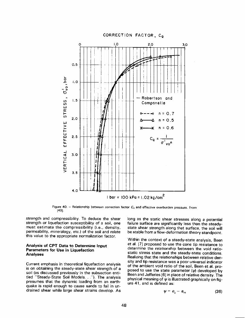
0.5
...C.0 1.0
0->b
(J) 1.5(J)
wa::.....(J)
2.0w>-r-uw 2.5lL.lL.W
-I<t 3.0u.....a::w> 3.5
~..I""--~""J...o.-""10'-I- - ~~,'-
~,I 1/
I~-Robertson and
--- Campanella
,()o--~ n = 0.7,tr----(). n = 0.5
I )( )( n = 0.6I,
ICQ = I
cr YOn,
I~rr,,
U
CORRECTION FACTORI CQ
0 1.0 3.02.0
4.02
I bar = 100 kPa = 1.02 kg/em
Figure 40. - Relationship between correction factor Co and effective overburden pressure. From[40].
strength and compressibility. To deduce the shearstrength or liquefaction susceptibility of a soil. onemust estimate the compressibility (i.e., density,permeability, mineralogy, etc.) of the soil and relatethis value to the appropriate normalization factor.
long as the static shear stresses along a potentialfailure surface are significantly less than the steady-state shear strength along that surface, the soil willbe stable from a flow-deformation theory standpoint.
Within the context of a steady-state analysis, Beenet al. [7] proposed to use the cone tip resistance todetermine the relationship between the void ratio-static stress state and the steady-state conditions.Realizing that the relationships between relative den-sity and tip resistance was a poor universal indicatorof the ambient void ratio of the soil. Been et al. pro-posed to use the state parameter (1jI) developed byBeen and Jefferies [6] in place of relative density. Thephysical meaning of If! is illustrated graphically on fig-ure 41, and is defined as:
Analysis of CPT Data to Determine InputParameters for Use in LiquefactionAnalyses
Current emphasis in theoretical liquefaction analysisis on obtaining the steady-state shear strength of asoil (as discussed previously in the subsection enti-tled "Steady-State Soil Models. . ."). The analysispresumes that the dynamic loading from an earth-quake is rapid enough to cause sands to fail in un-drained shear while large shear strains develop. As If! = e.. - ess (36)
48
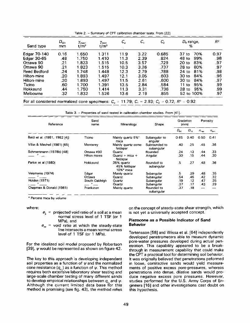
Table2. - Summary of CPT calibration chamber tests. From [22].
05°' Ymax' Yminl Co C, C2 DR range, R2Sand type mm t/m3 t/m3 %
Edgar 70-140 0.16 1.650 1.311 11.9 3.22 0.685 37 to 70% 0.97Edgar 30-65 .48 1.750 1.410 11.3 2.39 .824 48 to 99% .98Ottawa 90 .21 1.823 1.515 10.5 3.57 .729 20 to 83% .97Ottawa 90 .21 1.823 1.515 10.3 3.26 .737 28 to 80% .97Reed Bedford .24 1.748 1.448 12.3 2.79 .788 24 to 81% .98Hilton-mine .20 1.893 1.497 12.1 3.05 .603 30 to 84% .96Hilton-mine .20 1.893 1.497 11.5 2.61 .600 30 to 84% .97Ticino .60 1.700 1.391 13.5 2.84 .584 11 to 95% .99Hokksund .44 1.750 1.414 11.3 3.31 .736 28 to 95% .99Melbourne .32 1.832 1.526 13.6 2.19 .855 52 to 100% .97
For all considered normalized cone specimens: Co = 11.79; C, = 2.93; C2 = 0.72; R2 = 0.92
Sand Gradation PorosityReference name Mineralogy Shape (mm)
060 010 nmax nmin
Baldi et al. (1981. 1982 [4]) Ticino Mainly quartz 5%* Subangular to 0.65 0.40 0.50 0.41mica angular
Villet & Mitchell (1981) [65] Monterey Mainly quartz some Subrounded to .40 .25 .45 .36feldspar subangular
Schmertmann (1978b) [48] Ottawa #90 Quartz Rounded .24 .13 .44 .33.. Hilton mines Quartz + mica + Angular .30 .15 .44 .30- -
feldsparParkin et al (1980) Hokksund 35% quartz Rounded to .5 .27 .48 .36
45% feldspar subangular10%* mica
Veismanis (1974) Edgar Mainly quartz Subangular .5 .29 .48 .35.. Ottawa Quartz Subangular .54 .45 .42 .32- -
Holden (1971) South Oakleigh Quartz Subangular .19 .12 .47 .35.. .. Quartz Subangular .37 .17 .43 .29- - - -
Chapman & Donald (1981) Frankston Mainly quartz Rounded to .37 .18subangular
Table 3. - Properties of sand tested in calibration chamber studies. From [41].
* Percent mica by volume
where:e.. = projected void ratio of a soil at a mean
normal stress level of 1 TSF (or 1MPa), and
ess = void ratio at which the steady-stateline intersects a mean normal stresslevel of 1 TSF (or 1 MPa).
For the idealized soil model proposed by Robertson[39], IfIwould be represented as shown on figure 42.
The key to this approach is developing independentsoil properties as a function of IfI and the normalizedcone resistance (qc ) as a function of 1fI.This methodrequires both exter1sive laboratory shear testing andlarge-scale chamber testing of many different sandsto develop empirical relationships between qc and 1fI.Although the current limited data base fbr thismethod is promising (see fig. 43), the method relies
on the concept of steady-state shear strength, whichis not yet a universally accepted concept.
Piezocone as a Possible Indicator of SandBehavior
Tortensson [58] and Wissa et al. [64] independentlydeveloped penetrometers able to measure dynamicpore-water pressures developed during actual pen-etration. This capability appeared to be a break-through in measurement capability that could makethe CPT a practical tool for determining soil behavior.It was originally believed that penetrations peformedin loose, contractive sands would yield measure-ments of positive excess pore-pressures, whereaspenetrations into dense, dilative sands would pro-duce negative excess pore pressures. However,studies performed for the U.S. Army Corps of En-gineers [16] and other investigations cast doubt onthis hypothesis.
49
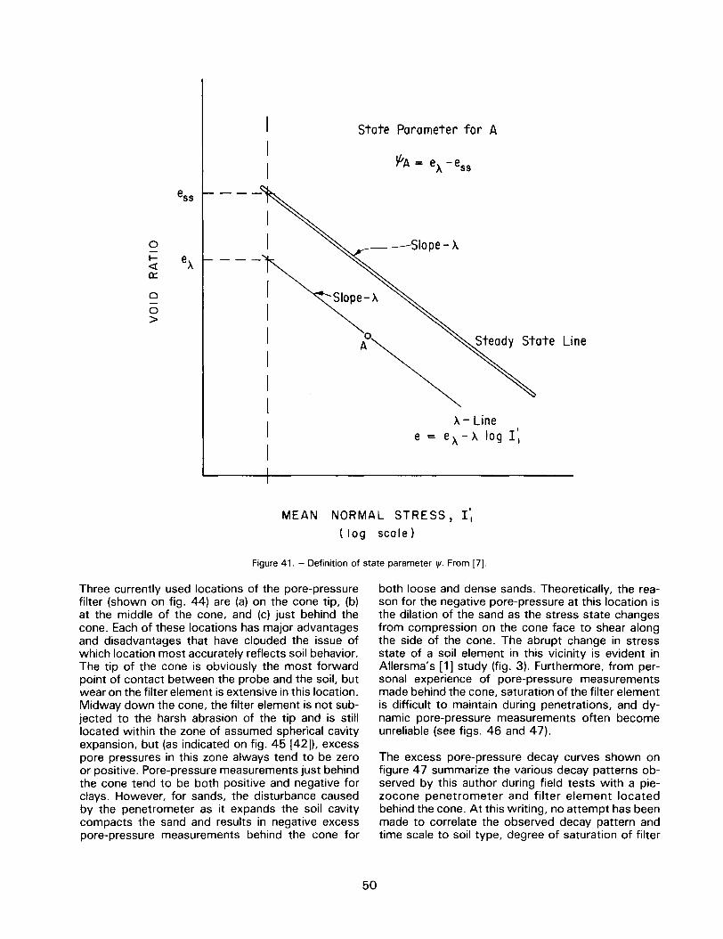
ess
0~<!:a::
eA ---
0
0>
State Parameter for A
'fA = eA -ess
Slope- A
A- Linee = eA-A log 1'1
MEAN NORMAL STRESS I 1'1(log scale)
Figure 41. - Definition of state parameter'll. From [7].
Three currently used locations of the pore-pressurefilter (shown on fig. 44) are (a) on the cone tip, (b)at the middle of the cone, and (c) just behind thecone. Each of these locations has major advantagesand disadvantages that have clouded the issue ofwhich location most accurately reflects soil behavior.The tip of the cone is obviously the most forwardpoint of contact between the probe and the soil. butwear on the filter element is extensive in this location.Midway down the cone, the filter element is not sub-jected to the harsh abrasion of the tip and is stilllocated within the zone of assumed spherical cavityexpansion, but (as indicated on fig. 45 [42]), excesspore pressures in this zone always tend to be zeroor positive. Pore-pressure measurements just behindthe cone tend to be both positive and negative forclays. However, for sands, the disturbance causedby the penetrometer as it expands the soil cavitycompacts the sand and results in negative excesspore-pressure measurements behind the cone for
both loose and dense sands. Theoretically, the rea-son for the negative pore-pressure at this location isthe dilation of the sand as the stress state changesfrom compression on the cone face to shear alongthe side of the cone. The abrupt change in stressstate of a soil element in this vicinity is evident inAllersma's [1] study (fig. 3). Furthermore, from per-sonal experience of pore-pressure measurementsmade behind the cone, saturation of the filter elementis difficult to maintain during penetrations, and dy-namic pore-pressure measurements ohen becomeunreliable (see figs. 46 and 47).
The excess pore-pressure decay curves shown onfigure 47 summarize the various decay patterns ob-served by this author during field tests with a pie-zocone penetrometer and filter element locatedbehind the cone. At this writing, no attempt has beenmade to correlate the observed decay pattern andtime scale to soil type, degree of saturation of filter
50
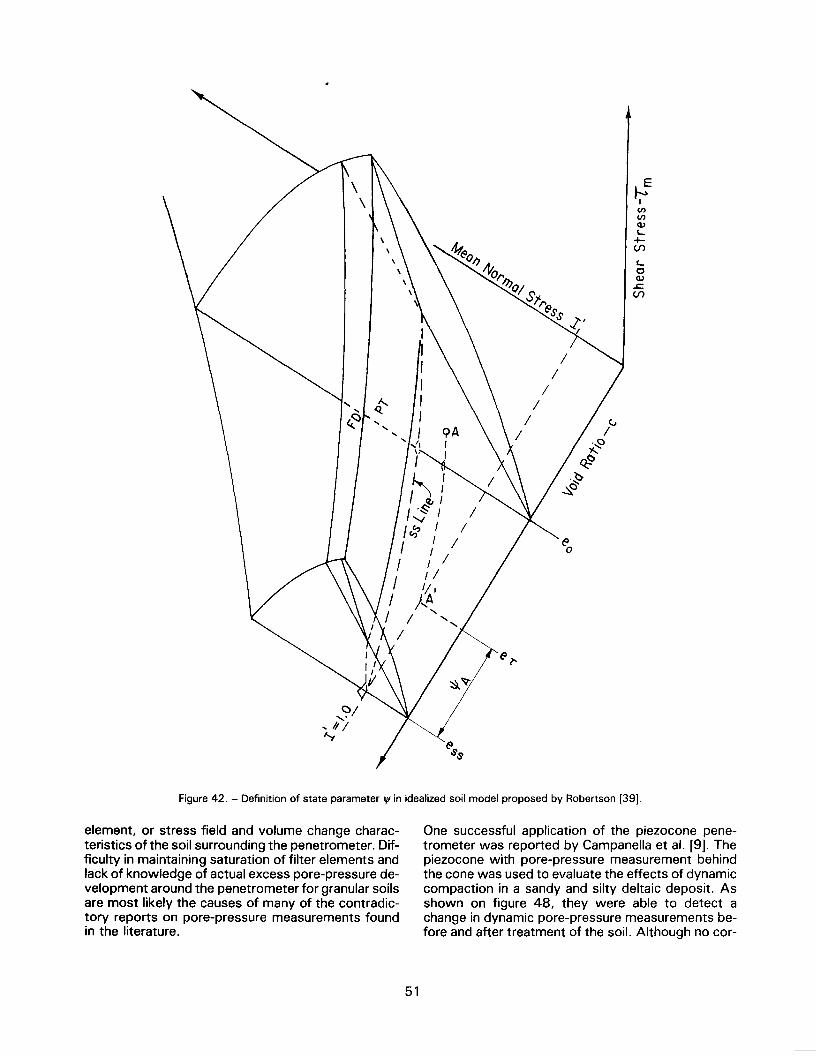
~EJVIVIQ)
l-+-(/)
I-0Q)
.s::.(/)
" <t'~~ v
/.C>~
~.~
~C>
Figure 42. - Definition of state parameter Ijf in idealized soil model proposed by Robertson [39].
element, or stress field and volume change charac-teristics of the soil surrounding the penetrometer. Dif-ficulty in maintaining saturation of filter elements andlack of knowledge of actual excess pore-pressure de-velopment around the penetrometer for granular soilsare most likely the causes of many of the contradic-tory reports on pore-pressure measurements foundin the literature.
One successful application of the piezocone pene-trometer was reported by Campanella et al. [9]. Thepiezocone with pore-pressure measurement behindthe cone was used to evaluate the effects of dynamiccompaction in a sandy and silty deltaic deposit. Asshown on figure 48, they were able to detect achange in dynamic pore-pressure measurements be-fore and after treatment of the soil. Although no cor-
51
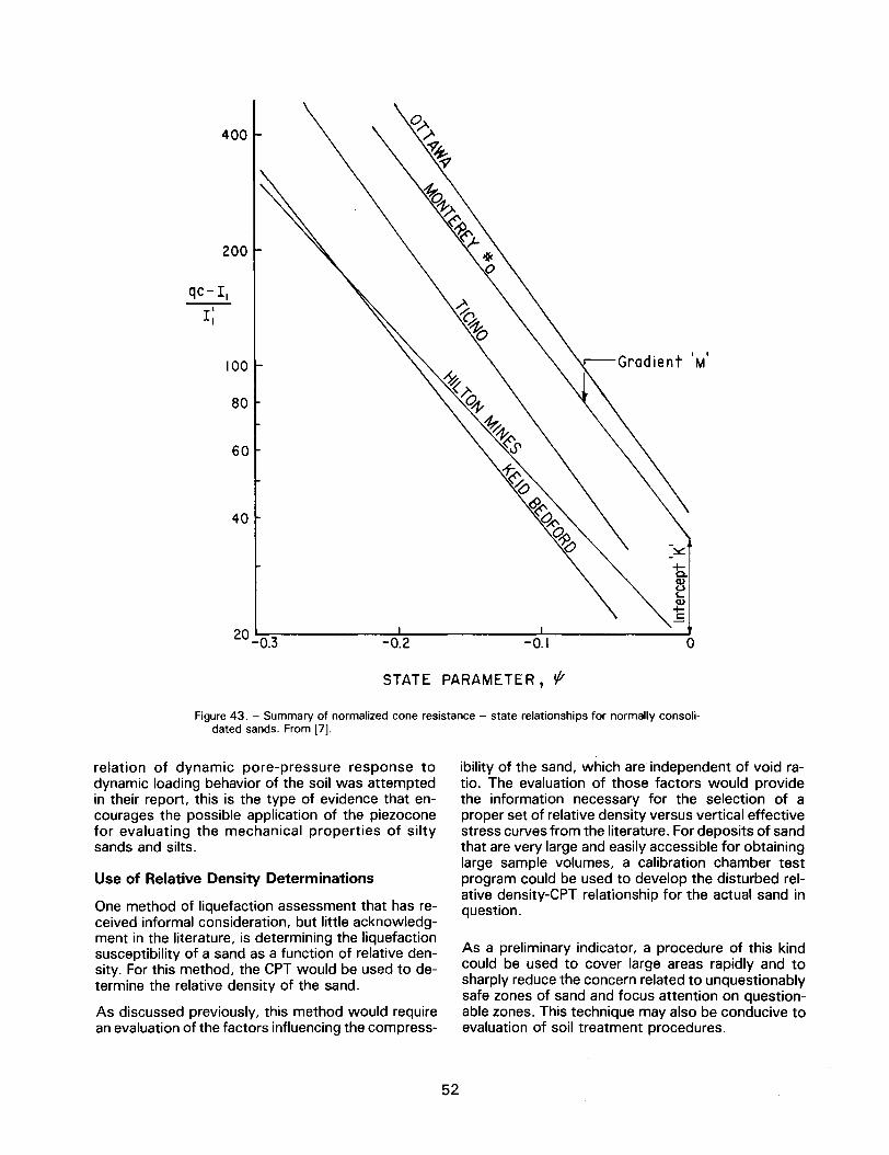
400
200
qC-II
III
100
80
60
40
20 -0.3 -0.2 -0.1 0
STATE PARAMETER, ~
Figure 43. - Summary of normalized cone resistance - state relationships for normally consoli-dated sands. From [7].
relation of dynamic pore-pressure response todynamic loading behavior of the soil was attemptedin their report, this is the type of evidence that en-courages the possible application of the piezoconefor evaluating the mechanical properties of siltysands and silts.
Use of Relative Density Determinations
One method of liquefaction assessment that has re-ceived informal consideration, but little acknowledg-ment in the literature, is determining the liquefactionsusceptibility of a sand as a function of relative den-sity. For this method, the CPT would be used to de-termine the relative density of the sand.
As discussed previously, this method would requirean evaluation of the factors influencing the compress-
ibility of the sand, which are independent of void ra-tio. The evaluation of those factors would providethe information necessary for the selection of aproper set of relative density versus vertical effectivestress curves from the literature. For deposits of sandthat are very large and easily accessible for obtaininglarge sample volumes, a calibration chamber testprogram could be used to develop the disturbed rel-ative density-CPT relationship for the actual sand inquestion.
As a preliminary indicator, a procedure of this kindcould be used to cover large areas rapidly and tosharply reduce the concern related to unquestionablysafe zones of sand and focus attention on question-able zones. This technique may also be conducive toevaluation of soil treatment procedures.
52

FilterElement
Filter Element
(c) Behind the cone element.(b) Face element(a) Ti p element.
Figure 44. - Location of filter elements for measurement of pore pressure.
. . . .' '. '.
Loose si I t(contractive)
Densesilt
(Dilative)
use,---
h:HOG~
FUGROf
Dense fine sand
1110
/',/
,/
/' Co.e. clay,;
/I
/I
/
?
vivoLoose fine sand
Figure 45. - Conceptual pore pressure distribution in saturated soil during cone penetration. From [42].
53
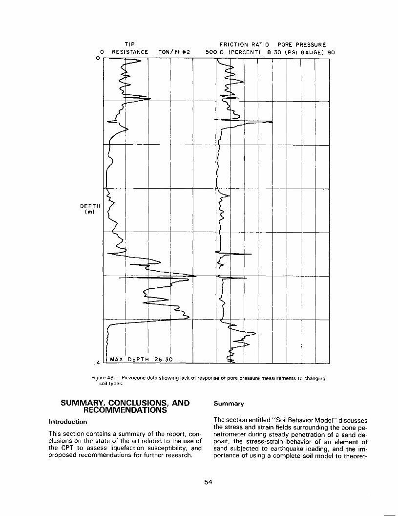
00
TIPRESISTANCE TON/ ft #2
FRICTION RATIO PORE PRESSURE500 D (PERCENT) 8-30 (PSI GAUGE) 90
DEPTH(m)
-f
14MAX DEPT H 26.30
Figure 46. - Piezocone data showing lack of response of pore pressure measurements to changingsoil types.
SUMMARY, CONCLUSIONS, ANDRECOMMENDATIONS
Summary
Introduction
This section contains a summary of the report, con-clusions on the state of the art related to the use ofthe CPT to assess liquefaction susceptibility, andproposed recommendations for further research.
The section entitled "Soil Behavior Model" discussesthe stress and strain fields surrounding the cone pe-netrometer during steady penetration of a sand de-posit, the stress-strain behavior of an element ofsand subjected to earthquake loading, and the im-portance of using a complete soil model to theoret-
54
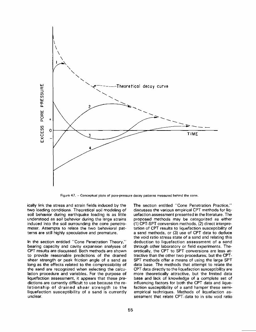
li.Ja:::::>CJ)CJ)li.Ja::Cl.
li.Ja::0Cl.
\\
\\
~"-
"-
"-.........
""~Theoretical"'- '-....
....................
..........
+
CJ)CJ)li.JUXli.J
0
decay curve
.................
-- -- ~ -- -- - -~----TIME
Figure 47. - Conceptual plots of pore-pressure decay patterns measured behind the cone.
ically link the stress and strain fields induced by thetwo loading conditions. Theoretical soil modeling ofsoil behavior during earthquake loading is as littleunderstood as soil behavior during the large strainsinduced into the soil surrounding the cone penetro-meter. Attempts to relate the two behavioral pat-terns are still highly speculative and premature.
In the section entitled "Cone Penetration Theory,"bearing capacity and cavity expansion analyses ofCPT results are discussed. Both methods are shownto provide reasonable predictions of the drainedshear strength or peak friction angle of a sand aslong as the effects related to the compressibility ofthe sand are recognized when selecting the calcu-lation procedure and variables. For the purpose ofliquefaction assessment, it appears that these pre-dictions are currently difficult to use because the re-lationship of drained shear strength to theliquefaction susceptibility of a sand is currentlyunclear.
The section entitled "Cone Penetration Practice,"discusses the various empirical CPT methods for liq-uefaction assessment presented in the literature. Theproposed methods may be categorized as either(1) CPT-SPT conversion methods, (2) direct interpre-tation of CPT results to liquefaction susceptibility ofa sand methods, or (3) use of CPT data to deducethe void ratio stress state of a sand and relating thisdeduction to liquefaction assessment of a sandthrough other laboratory or field experiments. The-oretically, the CPT to SPT conversions are less at-tractive than the other two procedures; but the CPT-SPT methods offer a means of using the large SPTdata base. The methods that attempt to relate theCPT data directly to the liquefaction susceptibility aremore theoretically attractive, but the limited database and lack of knowledge of a complete set ofinfluencing factors for both the CPT data and lique-faction susceptibility of a 'sand hamper these semi-empirical techniques. Mefhods of liquefaction as-sessment that relate CPT, data to in situ void ratio
55
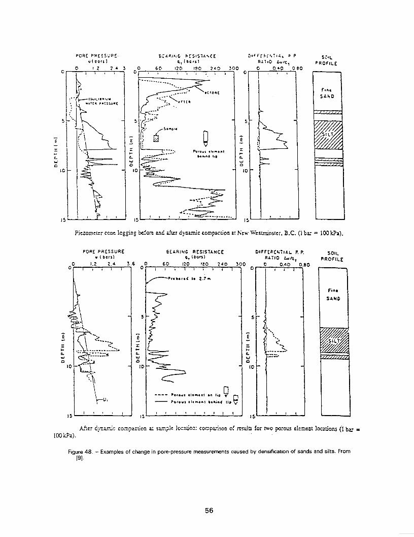
=
PORE P~E~~::?~,,( too" )
0 1.2 2.'" ~0~..
..
~..~{~,,,..,~..... i~ ."T(a. '~~~1U.C
,<J.J
(\\...\...
~
""c\
~~
~~~
10
I~
00
HL":",c; F<fStS1l."CE~,(~O..)
6e 120 I~O 2LO ~OO
=...Co.
""c10
0
~,~rc;.:..,,:.l...L ~ PFI~110 Lu'"0 OLO oeo
S,.!\.PRor'lE
r,,,.
S:''''D
Pj~zom:t::r CCD~Jegging ~fOR 2.!1d,,~r dYDamic compaction ,! J'.;~w W~stminst~., B.C. (1 bar = JOO kPa).
00
PORE PRESSUREu ( bO")
U 2'"~.6
E
=
Ui
I~
E
1t'00'
~
00
HARING RESISTANCEq,lt>or1)
60 120 !eO 2LOI
OtHER(liTIAL P. P.Rt..TIO t...IQT
~OO 0 O.LO 0.800 I
SOIl.P-ROFllE
56
E
I~
sr-
E-"" ",
~ ':;.\I.__n~,1--:=..
~ .
...............
';'~.~'" ""~ r-r [.;.'\.,.." ~ .
-:;'''...'''.'''~.;..:~~
~~o"'''~
~ Q
=...Co.\oJ0
10
I~
Fi".SAND
-
-
1
M:. dY1:2..mi: CO:TIp2.::tjODa: s::"'7l?k JO::uiOil: cornp::..-ison of r:suJrs for two porous d:c:nt lo z.uons (1 bzr =100kPc).
= P-orOll1 t~,"t
~. hI"" 'I~
Figure 48. - Examples of change in pore-pressure measurements caused by densification of sands and silts. From[9].
...Co.
""010
I:>.."
"''''''..I ,
5
E
=
"oro.., lit ,,' 0" tOpQ0
~o,.,,' el, ", ~.hi"4 Ii, V
I~
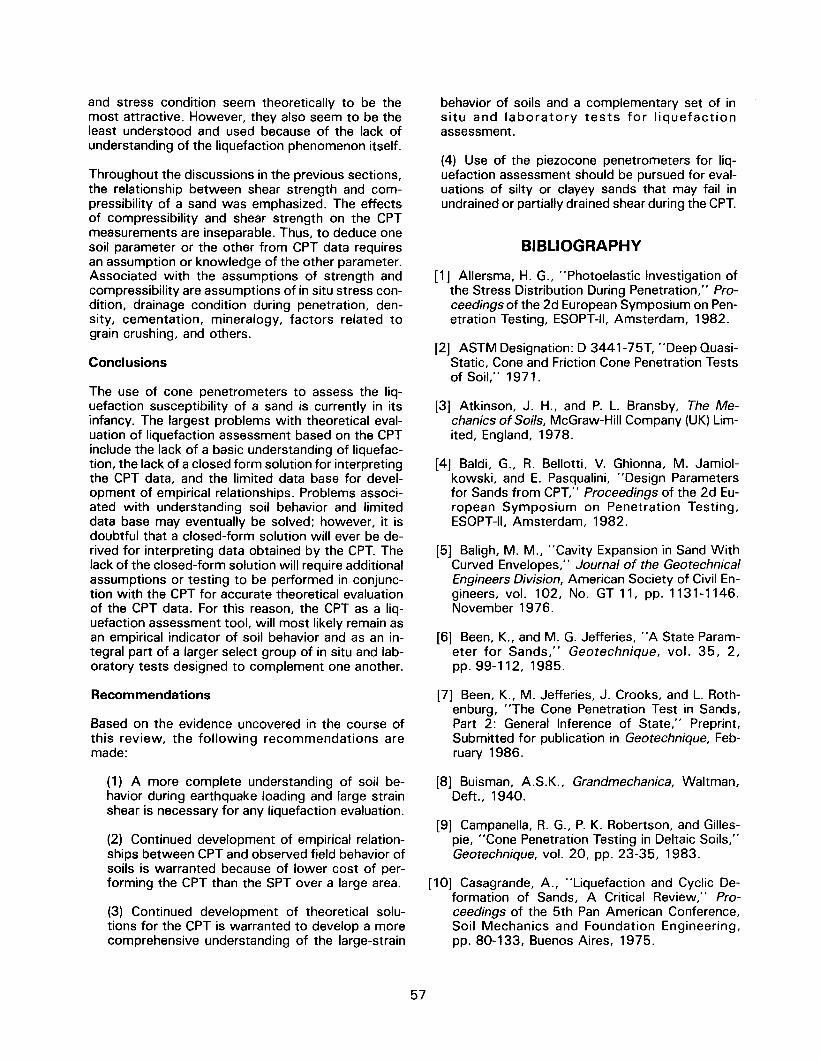
and stress condition seem theoretically to be themost attractive. However, they also seem to be theleast understood and used because of the lack ofunderstanding of the liquefaction phenomenon itself.
Throughout the discussions in the previous sections,the relationship between shear strength and com-pressibility of a sand was emphasized. The effectsof compressibility and shear strength on the CPTmeasurements are inseparable. Thus, to deduce onesoil parameter or the other from CPT data requiresan assumption or knowledge of the other parameter.Associated with the assumptions of strength andcompressibility are assumptions of in situ stress con-dition, drainage condition during penetration, den-sity, cementation, mineralogy, factors related tograin crushing, and others.
Conclusions
The use of cone penetrometers to assess the liq-uefaction susceptibility of a sand is currently in itsinfancy. The largest problems with theoretical eval-uation of liquefaction assessment based on the CPTinclude the lack of a basic understanding of liquefac-tion, the lack of a closed form solution for interpretingthe CPT data, and the limited data base for devel-opment of empirical relationships. Problems associ-ated with understanding soil behavior and limiteddata base may eventually be solved; however, it isdoubtful that a closed-form solution will ever be de-rived for interpreting data obtained by the CPT. Thelack of the closed-form solution will require additionalassumptions or testing to be performed in conjunc-tion with the CPT for accurate theoretical evaluationof the CPT data. For this reason, the CPT as a liq-uefaction assessment tool, will most likely remain asan empirical indicator of soil behavior and as an in-tegral part of a larger select group of in situ and lab-oratory tests designed to complement one another.
Recommendations
Based on the evidence uncovered in the course ofthis review, the following recommendations aremade:
(1) A more complete understanding of soil be-havior during earthquake loading and large strainshear is necessary for any liquefaction evaluation.
(2) Continued development of empirical relation-ships between CPT and observed field behavior ofsoils is warranted because of lower cost of per-forming the CPT than the SPT over a large area.
(3) Continued development of theoretical solu-tions for the CPT is warranted to develop a morecomprehensive understanding of the large-strain
behavior of soils and a complementary set of insitu and laboratory tests for liquefactionassessment.
(4) Use of the piezocone penetrometers for liq-uefaction assessment should be pursued for eval-uations of silty or clayey sands that may fail inundrained or partially drained shear during the CPT.
BIBLIOGRAPHY
[1] Allersma, H. G., "Photoelastic Investigation ofthe Stress Distribution During Penetration," Pro-ceedings of the 2d European Symposium on Pen-etration Testing, ESOPT-II, Amsterdam, 1982.
[2] ASTMDesignation: D 3441-75T, "Deep Quasi-Static, Cone and Friction Cone Penetration Testsof Soil:' 1971.
[3] Atkinson, J. H., and P. L. Bransby, The Me-chanics of Soils, McGraw-Hili Company (UK) lim-ited, England, 1978.
[4] Baldi, G., R. Bellotti, V. Ghionna, M. Jamiol-kowski, and E. Pasqualini, "Design Parametersfor Sands from CPT," Proceedings of the 2d Eu-ropean Symposium on Penetration Testing,ESOPT-II, Amsterdam, 1982.
[5] Baligh, M. M., "Cavity Expansion in Sand WithCurved Envelopes:' Journal of the GeotechnicalEngineers Division, American Society of Civil En-gineers, vol. 102, No. GT 11, pp.1131-1146.November 1976.
[6] Been, K., and M. G. Jefferies, "A State Param-eter for Sands," Geotechnique, vol. 35, 2,pp. 99-112, 1985.
[7] Been, K., M. Jefferies, J. Crooks, and L. Roth-enburg, "The Cone Penetration Test in Sands,Part 2: General Inference of State:' Preprint,Submitted for publication in Geotechnique, Feb-ruary 1986.
[8] Buisman, A.S.K., Grandmechanica, Waltman,Deft., 1940.
[9] Campanella, R. G., P. K. Robertson, and Gilles-pie, "Cone Penetration Testing in Deltaic Soils,"Geotechnique, vol. 20, pp. 23-35, 1983.
[10] Casagrande, A., "Liquefaction and Cyclic De-formation of Sands, A Critical Review:' Pro-ceedings of the 5th Pan American Conference,Soil Mechanics and Foundation Engineering,pp. 80-133, Buenos Aires, 1975.
57
[11] Castro, G., "Liquefaction of Sands," Ph.D. Dis-sertation, Division of Engineering and AppliedPhysics, Harvard University, 1969.
[12] Castro, G., "Liquefaction and Cyclic Mobility ofSaturated Sands," Journal of the GeotechnicalEngineering Division, American Society of CivilEngineers, vol. 101, No. GT6, pp. 551-569, June1975.
[13] Castro, G., and S. J. Poulos, "Factors AffectingLiquefaction and Cyclic Mobility," Journal of theGeotechnical Engineering Division, American So-ciety of Civil Engineers, vol. 106, No. GT6, pp.501-505, 1977.
[14] "Cone Penetration Testing and Experience,"Proceedings of a Session Sponsored by the Geo-technical Division, National Convention, Ameri-can Society of Civil Engineers, St. Louis, MO,October 1981.
[15] Cooper, S. S., and A. G. Franklin, "PQS ProbeSimultaneous Measurement of Penetration Re-sistance and Pore Pressure," Final Report GL-82-8, U.S. Army Corps of Engineers, WaterwaysExperiment Station, Vicksburg, MS, September1982.
[16] Douglas, B. J., and R. S. Olsen, "Soil Classifi-cation using Electric Cone Penetrometer," Sym-posium on Cone Penetration Testing andExperience, Geotechnical Engineering Division,ASCE, pp. 209-227, St. Louis, MO, 1981.
[17] Durgunoglu, H. T, and J. K. Mitchell, "StaticPenetration Resistance of Soils: I-Analysis," Pro-ceedings, Specialty Conference on In Situ Meas-urement of Soil Properties, American Society ofCivil Engineers, Raleigh, NC, 1975.
[18] Farrar, J. A., "Study of In Situ Testing for Eval-uation of Liquefaction Resistance and Occur-rence," Bureau of Reclamation, Special TechnicalReport, (in draft), 1986.
[19] Ferritto, J. M., and R. T Nakamoto, "A Sum-mary of the Prevost Effective Stress Soil Mode,"Technical Report R-913, Naval Civil EngineeringLaboratory, Port Hueneme, CA, October 1984.
[20] Harris, W. G., J. C. Parker, and L. W. Zelazny,"Effects of Mica Content on Engineering Prop-erties of Sand," Journal of Soil Science Societyof America, vol. 48, No.3, pp. 501-505, 1984.
[21] "In Situ Measurement of Soil Properties", Pro-ceedings of the Specialty Conference of Geo-technical Division, American Society of CivilEngineers, Raleigh, NC, June 1975.
[22] Jamiolkowski, M., G. Baldi, R. Bellotti, V.Ghionna, and E. Pasqualini, "Penetration Resist-ance and Liquefaction of Sands," Proceedings,11th International Conference on Soil Mechanicsand Foundation Engineering, vol. 4, pp. 1891-1896, 1985.
[23] Janbu, N., and K. Senneset, "Effective StressInterpretation of In Situ Static Penetration Tests,"Proceedings of the European Symposium on Pen-etration Testing:' Stockholm, Sweden, vol. 2.2,pp. 181-193, 1975.
[24] Levadoux, J. N., and M. M. Baligh, "Pore Pres-sures During Cone Penetration in Clays," Mas-sachusetts Institute of Technology, Departmentof Civil Engineering, publication No. R80-15, April1980.
[25] Liquefaction of Soils During Earthquakes, Re-port from the Committee on Earthquake Engi-neering, National Research Council, NationalAcademy Press, Washington, D.C., 1985.
[26] Lunne, T, and H. P. Christoffersen, "Interpre-tation of Cone Penetrometer Data for OffshoreSands," Norwegian Geotechnical Institute, Pub-lication No. 156, Olso, Norway, 1985.
[27] Lunne, T, T Eidsmoen, D. Gillespie, and J. D.Howland, "Laboratory and Field Evaluation ofCone Penetrometers:' Use of In Situ Tests inGeotechnical Engineering, Proceedings of In Situ'86, a Specialty Conference Sponsored by theGeotechnical Division of the American Society ofCivil Engineers, Geotechnical special publicationNo.6, pp. 714-729. Blacksburg, VA, 1986.
[28] Matsuoka, H., "Stress-Strain Relationships ofSands Based on the Mobilized Plane," SoilsFoundations, vol. 14, pp. 47-61,1974.
[29] Meyerhof, G. G. "The Ultimate Bearing Capac-ity of Wedge-Shaped Foundations," Proceedingsof the 5th International Conference of Soil Me-chanics and Foundation Engineering, vol. 2, pp.105-109, Paris, 1961.
[30] Mitchell, J. K., and J. M. Keaveny, "DeterminingSand Strength by Cone Penetrometer:' Use ofIn Situ Tests in Geotechnical Engineering, Pro-ceedings of In Situ '86, a Specialty ConferenceSponsored by the Geotechnical Division of theAmerican Society of Civil Engineers, Geotech-nical Special Publication No.6, pp. 823-839,Blacksburg, VA, 1986.
[31] Nagase, H., "Behavior of Sand in a Multidirec-tionallrregular Loading," Ph.D. Dissertation, De-partment of Civil Engineering, University ofTokyo, Japan, 1985.
58
[32] Olsen, R. S., "LiquefactionAnalysis Using theCone Penetrometer Test," Proceedings of the8th World Conference on Earthquake Engineer-ing, San Francisco, CA, July 1984.
[33] Poorooshasb, H. B., I. Holubec, and A. N. Sher-bourne, "Yield and Flow of Sand in TriaxialCompression," Canadian Geotechnical Journal,Part 1,3, pp. 179-190, 1966; Parts 2 and 3, 4,pp. 376-397, 1966/67.
[34] Poorooshasb, H. B., and S. Pietruszczak, "AGeneralized Flow Theory for Sand," Soils anFoundations, Japanese Society of Soil Mechan-ics and Foundation Engineering, vol. 26, No.2,1986.
[35] Poulos, S. J., "The Steady-State of Deforma-tion:' Journal of Geotechnical Engineering,American Society of CivilEngineers, vol. 107,5,pp. 553-562, pp. 1-15, June 1981.
[36] Proceedings of the European Symposium onPenetration Testing, ESOPT-I,Swedish Geotech-nical Society, Stockholm, Sweden, June 1974.
[37] Proceedings of the Second European Sympos-ium on Penetration Testing, ESOPT-II, Amster-dam, Holland, May 1982.
[38] "Report of the Subcommittee on Standardiza-tion of Penetration Testing in Europe", Interna-tional Society of Soil Mechanics and FoundationEngineering, Proceedings of the 9th InternationalConference on Soil Mechanics and FoundationEngineering, Tokyo, Japan, 1977.
[39] Robertson, P. K., "In Situ Testing of Soil WithEmphasis on Its Application to Liquefaction As-sessment:' Ph.D. Dissertation, Department ofCivilEngineering, University of British Columbia,Vancouver, Canada, 1983.
[40] Robertson, P. K., and R. G. Campanella, "Inter-pretation of Cone Penetration Tests - Part I(Sand)," Canadian Geotechnical Journal, vol. 20,No.4, 1983.
[41] Robertson, P. K., and R. G. Campanella, "Guide-lines for Use and Interpretation of the ElectronicCone Penetration Test," Soil Mechanics SeriesNo. 69, Department of Civil Engineering, Univer-sity of British Columbia, Vancouver, Canada, Jan-uary 1984.
[42] Robertson, P. K., R. G. Campanella, D. Gillespie,and J. Greig, "Use of Piezometer Cone Data,"Use of In Situ Tests in Geotechnical Engineering,a specialty conference sponsored by the Geo-
technical Division of the American Society of CivilEngineers, Geotechnical special publication No.6, pp. 1263-1280, Blacksburg, VA, 1986.
[43] Robertson, P. K., R. G. Campanella, and A.Wightman, "SPT-CPT Correlations," Soil Me-chanics Series No. 62, Department of Civil En-gineering, University of British Columbia,Vancouver, Canada, October 1982.
[44] Rowe, P. W., "The Stress-Dilatancy Relation forStatic Equilibriumof an Assembly of Particles inContact:' Proceedings, Royal Society, vol. 269,series A, pp. 500-527, 1962.
[45] Sanglerat, G., The Penetrometer and Soil Ex-ploration, Elsevier, 1972.
[46] Schmertmann, J. H., "Predicting the Qc!N Ra-tio:' Final Report 0-636, Engineering and Indus-trial Experiment Station, Department of CivilEngineering, University of Florida, Gainesville, FL,1976.
[47] Schmertmann, J. H., "Guidelines for Cone Pen-etration Test, Performance and Design:' FederalHighway Administration, Report FHWA-TS-78-209, Washington, D.C., July 1978.
[48] Scott, R. F., "Plasticity and Constitutive Rela-tions in Soil Mechanics," 19th Terzaghi Lecture,Journal of Geotechnical Engineering, AmericanSociety of Civil Engineers, vol. 111, No.5, pp.559-605, May 1985.
[49] Seed, H. B., "Some Aspects of Sand liquefac-tion Under Cyclic Loading," Proceedings, Con-ference on Behavior of Off-Shore Structures, theNorwegian Institute of Technology, Norway,1976.
[50] Seed, H. B., "Soil Liquefaction and Cyclic Mo-bility Evaluation for Level Ground During Earth-quakes:' Journal of the Geotechnical EngineeringDivision, American Society of Civil Engineers,vol. 105, No. GT2, pp. 201-255, February 1979.
[51] Seed, H. B., and I. M. Idriss, "Ground Motionsand Soil Liquefaction During Earthquakes," Earth-quake Engineering Research Institute, Mono-graph Series, Berkeley, CA, 1982.
[52] Seed, H. B., I. M. Idriss, and I. Arango, "Eval-uation of Liquefaction Potential Using Field Per-formance Data," Journal of GeotechnicalEngineering, American Society of Civil Engineers,vol. 109, No.3, pp. 458-482, March 1983.
59
[53] Seed, H. B., and P. De Alba, "Use of SPT andCPT Tests for Evaluating the Liquefaction Re-sistance of Sands," Use of In Situ Tests in Geo-technical Engineering, a Specialty ConferenceSponsored by the Geotechnical Division of theAmerican Society of CivilEngineers, Special Pub-lication No.6, pp. 281-302, Blacksburg, VA,1986.
[54] Shibata, T., H. Yukitomo, M. Miyoshi, "Lique-faction Process of Sand During Cyclic Loading,"Soils and Foundations, vol. 12, No.1, pp. 1-16,1972.
[55] Tatsuoka, F., "Shear Tests in a Triaxial Appa-ratus - A Fundamental Study of the Deformationof Sand," Ph.D. Dissertation, Tokyo University,Tokyo, Japan, 1972.
[56] Tatsuoka, F., and K. Ishihara, "Stress Path andDilatancy Performance of a Sand," Proceedings,8th International Conference on Soil Mechanicsand Foundation Engineering, vol. 1, pp. 419-424,Moscow, 1973.
[57] Terzaghi, K., Theoretical Soil Mechanics, J.Wiley and Sons, New York, NY, 1943.
[58] Tortensson, B. A., "Pore Pressure Sounding In-strument:' Discussion Session I. Proceedings,American Society of Civil Engineers Special Con-ference on In Situ Measurement of Soil Proper-ties, vol. II, pp. 48-54, Raleigh, NC, 1975.
[59] "Use of In Situ Tests in Geotechnical Engineer-ing", Proceedings of In Situ '86, a Specialty Con-ference Sponsored by the Geotechnical Divisionof the American Society of CivilEngineers, Geo-
technical Special Publication No.6, Blacksburg,VA, 1986.
[60] Vesic, A. S., "Expansion of Cavities in InfiniteSoil Masses," Journal of the Soil Mechanics andFoundationDivision, American Society of CivilEngineers, 98, SM3, pp. 265-290, 1972.
[61] Vesic, A. S., "Principles of Pile Design:' Lec-ture Series on Deep Foundations, Sponsored bythe Geotechnical Group, Boston Society of CivilEngineers Section, American Society of Civil En-gineers, in Cooperation with Massachusetts In-stitute of Technology, Cambridge, MA, 1975.
[62] Vesic, A. S., "Design of Pile Foundations:' Na-tional Cooperation Highway Research Program,Report No. 42, Transportation Research Board,Washington, D.C., 1977.
[63] Villet, W. C. B., and J. K. Mitchell (1981), "ConeResistance, Relative Density, and Friction An-gie:' Symposium on Cone Penetration Testingand Experience, Geotechnical Engineering Divi-sion, American Society of Civil Engineers, St.Louis, MO, October 1981.
[64] Wissa, A. E. Z., and R. T. Martin, and J. E.Garlanger, "The Piezometer Probe:' Proceed-ings, American Society of Civil Engineers Spe-cialty Conference in In Situ Measurement of SoilProperties, vol. I, pp. 536-545, Raleigh, NC,1975.
[65] Wroth, C. P.. "The Interpretation of In Situ SoilTests:' Geotechnique, vol. 34, No.4, pp. 449-489, 1984.
60 GPO 856--410
Mission of the Bureau of Reclamation
The Bureau of Reclamation of the U.S. Department of the Interior is responsible for ~e development and conservation of the Nation's water resources in the Western United States.
The Bureau's original purpose "to provide for the reclamation of arid and semiarid lands in the West" today covers a wide range of interre- la ted functions. These include providing municipal and industrial water supplies; hydroelectric power generation; irrigation water for agricul- ture; water quality improvement; flood control; river navigation; river regulation and control; fish and wildlife enhancement; outdoor recrea- tion; and research on water-rela ted design, construction, materials, atmospheric management, and wind and solar power.
Bureau programs most frequently are the result of close cooperation with the U.S. Congress, other Federal agencies, Stares, local govern- men ts, academic institutions, water-user organizations, and other concerned groups.
A free pamphlet is available from the Bureau entitled "Publications for Sale." I t describes some of the technical publications currently available, their cost, and how to order them. The pamphlet can be obtained upon request from the Bureau of Reclamation, Attn D-7923A. P 0 Box 25007, .Denver Federal Center, Denver CO 80225-0007.