Embed Size (px)
Citation preview

Report No. CCEER 14-04
NONLINEAR EVALUATION OF THE PROPOSED
SEISMIC DESIGN PROCEDURE FOR STEEL
BRIDGES WITH DUCTILE END CROSS FRAMES
Eric V. Monzon
Ahmad M. Itani
Michael A. Grubb
Center for Civil Engineering Earthquake Research
University of Nevada, Reno
July 2014


iii
Abstract
Neither the AASHTO LRFD Bridge Design Specifications nor the AASHTO Guide Specification for
LRFD Seismic Bridge Design provides a design procedure to achieve the desired seismic performance of
essentially elastic substructure and ductile superstructure. This Type 2 design strategy in the Guide
Specifications limits the inelastic activity to the superstructure of steel plate girder bridges. Due to the
lack of these specifications, bridge engineers have been reluctant of using this strategy which will only
limit the damage to the support cross frames in steel plate girder bridges. This controlled damage will
keep the substructure essentially elastic and thus limit its repair after a major earthquake.
This report presents a proposed ‘force-based’ design procedure that will achieve an essentially elastic
substructure and ductile superstructure. The reinforced concrete (R/C) substructure flexural resistance is
designed for the combined effect of seismic forces similar to conventional seismic design with a force
reduction factor equal to 1.5. Meanwhile, the shear resistance and the confinement requirements of the
substructure are determined in a way similar to the seismic design of conventional bridges. To achieve a
ductile superstructure, the horizontal resistance of the support cross frames is based on the lesser of the
pier nominal shear resistance and the elastic seismic cross forces obtained from the response spectrum
analysis, divided by a proposed response modification factor for ductile cross frames equal to 4. This will
ensure that support cross frames will act as a ‘fuse’ and will not subject the substructure to forces that
may cause nonlinear response in that direction. To achieve a ductile response of support cross frames, the
diagonal members, which are expected to undergo inelastic response, are detailed to have limits on width-
to-thickness and slenderness ratios. The other cross frame components and the shear resistance of the
substructure are then checked for a fully yielded and strain hardened support cross frame.
Three bridges were selected to illustrate the proposed design procedure for Type 2 design strategy. The
substructure of these bridges included single-column pier, two-column pier, and wall piers. Examples
showing the design of these bridges using conventional Type 1 design strategy with Critical and other
Operational Categories are also shown. Thus, a total of eight bridge design examples are shown in this
report. The proposed design strategy for Type 2 design showed an increase in the size of the substructure
when compared to ‘Other’ bridge operational category. However, it showed a decrease in the size of the
substructure when compared to ‘Critical’ bridge operational category. The seismic performance was
evaluated through nonlinear response history analysis using fourteen ground motions representing the
design and maximum considered earthquakes. The nonlinear seismic evaluation showed the Type 2
design strategy has indeed achieved an essentially elastic substructure and ductile superstructure as
intended to. It also showed that bridges with stiff substructure designed according to Type 1 strategy
have an inelastic activity in the superstructure. This will subject the connections and bearings to seismic
forces that they are not designed for, which may result in undesirable seismic performance. Thus utilizing
Type 2 design strategy for bridges with stiff substructure, i.e. pier wall, will offer great advantages by
limiting the lateral seismic forces and having a ‘fuse’ to dissipate the input energy. This will reduce the
seismic forces on the bearings and thus will lower the foundation cost.

iv
Acknowledgement
The work in this report was funded by American Iron and Steel Institute, AISI, contract CC-3070. Mr.
Dan Snyder was contract manager of which the authors sincerely appreciate his support and collaboration.
The authors appreciate the comments by a task group funded by AASHTO to support HSCOBS Technical
Committee on Seismic Design. The chair of this group is Dr. Lee Marsh. The authors wish to thank the
following individuals for their help and suggestions: Mr. Richard Pratt, Prof. Ian Buckle, Dr. Elmer Marx,
Dr. John Kulicki, Dr. Lian Duan, Mr. Greg Perfetti, Mr. Keith Fulton, and Dr. Gichuru Muchane.
Disclaimer
The materials set fourth here in are for general information only. They are not a substitute for competent
professional assistance. The opinions expressed in this report are those of the authors and do not
necessarily represents the views of the University of Nevada, Reno, the American Iron and Steel Institute
and the individuals who kindly provided the authors information and comments.

v
Table of Contents
Abstract ........................................................................................................................................................ iii
Acknowledgement ....................................................................................................................................... iv
Disclaimer .................................................................................................................................................... iv
Table of Contents .......................................................................................................................................... v
List of Tables ............................................................................................................................................... ix
List of Figures .............................................................................................................................................. xi
Chapter 1 Introduction ............................................................................................................................... 1
1.1 Background ................................................................................................................................... 1
1.2 Proposed AASHTO LRFD Bridge Design Specifications on Type 2 Design Strategy ................ 1
1.3 Seismic Design Examples ........................................................................................................... 16
1.3.1 Set I Bridges ........................................................................................................................ 16
1.3.2 Set II Bridges ...................................................................................................................... 17
1.3.3 Set III Bridges ..................................................................................................................... 18
1.4 Seismic Design Methodology ..................................................................................................... 19
1.5 Presentation of Design Examples ............................................................................................... 21
1.6 Analytical Model ........................................................................................................................ 21
1.6.1 Material Properties .............................................................................................................. 21
1.6.2 Superstructure ..................................................................................................................... 22
1.6.3 Cross Frames ....................................................................................................................... 24
1.6.4 Pier Caps and Columns ....................................................................................................... 24
1.6.5 Abutment Backfill Soil ....................................................................................................... 25
1.7 Design Loads .............................................................................................................................. 25
1.8 Seismic Evaluation of Design Examples .................................................................................... 29
1.8.1 Ground Motions .................................................................................................................. 29
1.8.2 Calculation of Column Yield Displacement ....................................................................... 33
1.8.3 Calculation of Superstructure Drift ..................................................................................... 36
Chapter 2 Bridge with Single-Column Piers Designed using Type 1 Strategy (Example I-1a) .............. 37
2.1 Bridge Description ...................................................................................................................... 37
2.2 Computational Model ................................................................................................................. 37
2.3 Analysis....................................................................................................................................... 38
2.3.1 Gravity Loads – DC and DW .............................................................................................. 38

vi
2.3.2 Earthquake Loads – EQ ...................................................................................................... 40
2.3.3 Design Loads ...................................................................................................................... 43
2.4 Design of Columns ..................................................................................................................... 44
2.5 Seismic Design of Cross-Frames ................................................................................................ 46
2.6 Cross-Frame Properties for Nonlinear Analysis ......................................................................... 49
2.7 Design Summary ......................................................................................................................... 51
2.8 Nonlinear Evaluation .................................................................................................................. 52
Chapter 3 Critical Bridge with Single-Column Piers Designed using Type 1 Strategy (Example I-1b) . 55
3.1 Bridge Description ...................................................................................................................... 55
3.2 Computational Model ................................................................................................................. 55
3.3 Analysis....................................................................................................................................... 56
3.3.1 Gravity Loads – DC and DW .............................................................................................. 56
3.3.2 Earthquake Loads – EQ ...................................................................................................... 58
3.3.3 Design Loads ...................................................................................................................... 61
3.4 Design of Columns ..................................................................................................................... 62
3.5 Seismic Design of Cross-Frames ................................................................................................ 64
3.6 Cross-Frame Properties for Nonlinear Analysis ......................................................................... 66
3.7 Design Summary ......................................................................................................................... 68
3.8 Nonlinear Evaluation .................................................................................................................. 69
Chapter 4 Bridge with Single-Column Piers Designed using Type 2 Strategy (Example I-2) ................ 72
4.1 Bridge Description ...................................................................................................................... 72
4.2 Computational Model ................................................................................................................. 72
4.3 Analysis....................................................................................................................................... 73
4.3.1 Gravity Loads – DC and DW .............................................................................................. 73
4.3.2 Earthquake Loads – EQ ...................................................................................................... 75
4.3.3 Design Loads ...................................................................................................................... 77
4.4 Design of Columns ..................................................................................................................... 78
4.5 Design of Ductile End Cross-Frames .......................................................................................... 81
4.6 Cross-Frame Properties for Nonlinear Analysis ......................................................................... 84
4.7 Design Summary ......................................................................................................................... 85
4.8 Nonlinear Evaluation .................................................................................................................. 86
Chapter 5 Bridge with Two-Column Piers Designed using Type 1 Strategy (Example II-1a) ............... 90
5.1 Bridge Description ...................................................................................................................... 90

vii
5.2 Computational Model ................................................................................................................. 90
5.3 Analysis....................................................................................................................................... 91
5.3.1 Gravity Loads – DC and DW .............................................................................................. 91
5.3.2 Earthquake Loads – EQ ...................................................................................................... 93
5.3.3 Design Loads ...................................................................................................................... 96
5.4 Design of Columns ..................................................................................................................... 97
5.5 Seismic Design of Cross-Frames .............................................................................................. 102
5.6 Cross-Frame Properties for Nonlinear Analysis ....................................................................... 104
5.7 Design Summary ....................................................................................................................... 105
5.8 Nonlinear Evaluation ................................................................................................................ 106
Chapter 6 Critical Bridge with Two-Column Piers Designed using Type 1 Strategy (Example II-1b) 109
6.1 Bridge Description .................................................................................................................... 109
6.2 Computational Model ............................................................................................................... 109
6.3 Analysis..................................................................................................................................... 110
6.3.1 Gravity Loads – DC and DW ............................................................................................ 110
6.3.2 Earthquake Loads – EQ .................................................................................................... 112
6.3.3 Design Loads .................................................................................................................... 115
6.4 Design of Columns ................................................................................................................... 116
6.5 Seismic Design of Cross-Frames .............................................................................................. 121
6.6 Cross-Frame Properties for Nonlinear Analysis ....................................................................... 123
6.7 Design Summary ....................................................................................................................... 125
6.8 Nonlinear Evaluation ................................................................................................................ 126
Chapter 7 Bridge with Two-Column Piers Designed using Type 2 Strategy (Example II-2) ............... 129
7.1 Bridge Description .................................................................................................................... 129
7.2 Computational Model ............................................................................................................... 129
7.3 Analysis..................................................................................................................................... 130
7.3.1 Gravity Loads – DC and DW ............................................................................................ 130
7.3.2 Earthquake Loads – EQ .................................................................................................... 132
7.3.3 Design Loads .................................................................................................................... 134
7.4 Design of Columns ................................................................................................................... 135
7.5 Design of Ductile Cross-Frames ............................................................................................... 140
7.6 Cross-Frame Properties for Nonlinear Analysis ....................................................................... 143
7.7 Design Summary ....................................................................................................................... 144

viii
7.8 Nonlinear Evaluation ................................................................................................................ 145
Chapter 8 Bridge with Wall Piers Design using Type 1 Strategy (Example III-1) ............................... 149
8.1 Bridge Description .................................................................................................................... 149
8.2 Computational Model ............................................................................................................... 149
8.3 Analysis..................................................................................................................................... 152
8.3.1 Gravity Loads – DC and DW ............................................................................................ 152
8.3.2 Earthquake Loads – EQ .................................................................................................... 152
8.3.3 Design Loads .................................................................................................................... 155
8.4 Design of Wall Pier ................................................................................................................... 156
8.5 Seismic Design of Cross-Frames .............................................................................................. 159
8.6 Cross-Frame Properties for Nonlinear Analysis ....................................................................... 161
8.7 Design Summary ....................................................................................................................... 162
8.8 Nonlinear Evaluation ................................................................................................................ 164
Chapter 9 Bridge with Wall Piers Designed using Type 2 Strategy (Example III-2) ............................ 167
9.1 Bridge Description .................................................................................................................... 167
9.2 Computational Model ............................................................................................................... 167
9.3 Analysis..................................................................................................................................... 170
9.3.1 Gravity Loads – DC and DW ............................................................................................ 170
9.3.2 Earthquake Loads – EQ .................................................................................................... 170
9.3.3 Design Loads .................................................................................................................... 173
9.4 Design of Wall Pier ................................................................................................................... 173
9.5 Design of Ductile Cross-Frames ............................................................................................... 177
9.6 Cross-Frame Properties for Nonlinear Analysis ....................................................................... 180
9.7 Design Summary ....................................................................................................................... 181
9.8 Nonlinear Evaluation ................................................................................................................ 182
Chapter 10 Summary of Design and Nonlinear Evaluation ................................................................ 186
10.1 Overview ................................................................................................................................... 186
10.2 Design Examples Summary ...................................................................................................... 186
10.3 Summary of Nonlinear Evaluations .......................................................................................... 188
10.3.1 Bridge with Single-Column Piers ..................................................................................... 188
10.3.2 Bridge with Two-Column Piers ........................................................................................ 189
10.3.3 Bridge with Wall Piers ...................................................................................................... 190
10.4 Concluding Remarks ................................................................................................................. 191

ix
References ................................................................................................................................................. 193
List of Tables
Table 1-1 Design examples ......................................................................................................................... 16
Table 1-2 Response modification factors .................................................................................................... 19
Table 1-3 Summary of nonlinear analyses runs .......................................................................................... 30
Table 2-1 Ex. I-1a superstructure equivalent concrete section properties .................................................. 37
Table 2-2 Modal periods and mass participation ........................................................................................ 41
Table 2-3 Column forces due to EQx .......................................................................................................... 42
Table 2-4 Column forces due to EQy .......................................................................................................... 42
Table 2-5 Combination of forces due to EQx and EQy ................................................................................ 43
Table 2-6 Design loads for columns ........................................................................................................... 43
Table 2-7 Design axial load and resultant moment ..................................................................................... 44
Table 3-1 Ex. I-1b superstructure equivalent concrete section properties .................................................. 55
Table 3-2 Modal periods and mass participation ........................................................................................ 59
Table 3-3 Column forces due to EQx .......................................................................................................... 60
Table 3-4 Column forces due to EQy .......................................................................................................... 60
Table 3-5 Combination of forces due to EQx and EQy ................................................................................ 61
Table 3-6 Design loads for columns ........................................................................................................... 61
Table 3-7 Design axial load and resultant moment ..................................................................................... 62
Table 4-1 Ex. I-2 superstructure equivalent concrete section properties .................................................... 72
Table 4-2 Modal periods and mass participation ........................................................................................ 76
Table 4-3 Column forces due to EQx .......................................................................................................... 77
Table 4-4 Column forces due to EQy .......................................................................................................... 77
Table 4-5 Design loads for columns ........................................................................................................... 77
Table 4-6 Design axial load and resultant moment ..................................................................................... 78
Table 5-1 Ex.II-1a superstructure section properties .................................................................................. 90
Table 5-2 Modal periods and mass participation ........................................................................................ 94
Table 5-3 Column forces due to EQx .......................................................................................................... 95
Table 5-4 Column forces due to EQy .......................................................................................................... 95
Table 5-5 Combination of forces due to EQx and EQy ................................................................................ 96
Table 5-6 Design loads for columns ........................................................................................................... 96
Table 5-7 Design axial load and resultant moment ..................................................................................... 97
Table 6-1 Ex.II-1b superstructure section properties ................................................................................ 109
Table 6-2 Modal periods and mass participation ...................................................................................... 113
Table 6-3 Column forces due to EQx ........................................................................................................ 114
Table 6-4 Column forces due to EQy ........................................................................................................ 114
Table 6-5 Combination of forces due to EQx and EQy .............................................................................. 115
Table 6-6 Design loads for columns ......................................................................................................... 115
Table 6-7 Design axial load and resultant moment ................................................................................... 116
Table 7-1 Ex.II-1 superstructure section properties .................................................................................. 129
Table 7-2 Modal periods and mass participation ...................................................................................... 133

x
Table 7-3 Column forces due to EQx ........................................................................................................ 134
Table 7-4 Column forces due to EQy ........................................................................................................ 134
Table 7-5 Design loads for columns ......................................................................................................... 134
Table 7-6 Design axial load and resultant moment ................................................................................... 135
Table 8-1 Ex.II-1 superstructure section properties .................................................................................. 149
Table 8-2 Modal periods and mass participation ...................................................................................... 153
Table 8-3 Column forces due to EQx ........................................................................................................ 154
Table 8-4 Column forces due to EQy ........................................................................................................ 154
Table 8-5 Combination of forces due to EQx and EQy .............................................................................. 155
Table 8-6 Design loads ............................................................................................................................. 155
Table 8-7 Design axial load and resultant moment ................................................................................... 156
Table 9-1 Ex.II-1 superstructure section properties .................................................................................. 167
Table 9-2 Modal periods and mass participation ...................................................................................... 171
Table 9-3 Column forces due to EQx ........................................................................................................ 172
Table 9-4 Column forces due to EQy ........................................................................................................ 172
Table 9-5 Design loads for wall pier ......................................................................................................... 173
Table 9-6 Design axial load and resultant moment ................................................................................... 173
Table 10-1 Summary of design ................................................................................................................. 187
Table 10-2 Summary of elastic seismic analysis ...................................................................................... 187
Table 10-3 Average column displacement ductility in bridges with single-column piers ........................ 188
Table 10-4 Average of total bearing force in the transverse direction ...................................................... 189
Table 10-5 Average column displacement ductility in bridges with two-column piers ........................... 190
Table 10-6 Average of total bearing force in the transverse direction ...................................................... 190
Table 10-7 Average of total bearing force in the transverse direction ...................................................... 191

xi
List of Figures
Figure 1-1 Plan view and cross-section of Set I bridges ............................................................................. 17
Figure 1-2 Plan view and cross-section of Set IIs and III bridges .............................................................. 18
Figure 1-3 Transformed sections used to calculate the equivalent section properties ................................ 26
Figure 1-4 Details of analytical model ........................................................................................................ 27
Figure 1-5 Force-displacement relationship of ductile cross-frames used for design evaluation ............... 28
Figure 1-6 Design spectrum ........................................................................................................................ 28
Figure 1-7. Comparison of design spectrum and geometric mean of spectra of selected records .............. 30
Figure 1-8 Response spectra of selected ground motions compared against design spectrum ................... 31
Figure 1-9 Response spectra of selected ground motions compared against MCE .................................... 32
Figure 1-10 Comparison of MCE spectrum and geometric mean of spectra of selected records ............... 33
Figure 1-11. Schematic diagram showing the column displacement .......................................................... 34
Figure 1-12. Forces in a single-column pier in the transverse direction. .................................................... 35
Figure 2-1 Elevation at piers of Ex. I-1a ..................................................................................................... 38
Figure 2-2 Analytical model of Ex. I-1a ..................................................................................................... 39
Figure 2-3 Abutment force-displacement ................................................................................................... 40
Figure 2-4 Column force-displacement plots from DE runs ....................................................................... 53
Figure 2-5 Column force-displacement plots from MCE runs ................................................................... 53
Figure 2-6 Summary of column Displacement ductility ............................................................................. 54
Figure 3-1 Elevation at piers of Ex. I-1b .................................................................................................... 56
Figure 3-2 Analytical model of Ex. I-1b ..................................................................................................... 57
Figure 3-3 Abutment force-displacement ................................................................................................... 58
Figure 3-4 Column force-displacement plots from DE runs ....................................................................... 70
Figure 3-5 Column force-displacement plots from MCE runs ................................................................... 70
Figure 3-6 Summary of column Displacement ductility ............................................................................. 71
Figure 4-1 Elevation at piers of Ex. I-2 ...................................................................................................... 73
Figure 4-2 Analytical model of Ex. I-2 ....................................................................................................... 74
Figure 4-3 Abutment force-displacement ................................................................................................... 75
Figure 4-4 Column force-displacement plots from DE runs ....................................................................... 87
Figure 4-5 Column force-displacement plots from MCE runs ................................................................... 87
Figure 4-6 Summary of column Displacement ductility ............................................................................. 88
Figure 4-7 Superstructure force-displacement in the transverse direction from DE runs ........................... 89
Figure 4-8 Superstructure force-displacement in the transverse direction from MCE runs ....................... 89
Figure 5-1 Elevation at pier of Ex. II-1a ..................................................................................................... 91
Figure 5-2 Analytical model of Ex. II-1a .................................................................................................... 92
Figure 5-3 Abutment force-displacement ................................................................................................... 93
Figure 5-4 Forces in a two-column pier ...................................................................................................... 99
Figure 5-5 Column force-displacement plots from DE runs ..................................................................... 107
Figure 5-6 Column force-displacement plots from MCE runs ................................................................. 107
Figure 5-7 Summary of column Displacement ductility ........................................................................... 108
Figure 6-1 Elevation at pier of Ex. II-1b ................................................................................................... 110
Figure 6-2 Analytical model of Ex. II-1b ................................................................................................. 111
Figure 6-3 Abutment force-displacement ................................................................................................. 112

xii
Figure 6-4 Forces in a two-column pier .................................................................................................... 118
Figure 6-5 Column force-displacement plots from DE runs ..................................................................... 127
Figure 6-6 Column force-displacement plots from MCE runs ................................................................. 127
Figure 6-7 Summary of column Displacement ductility ........................................................................... 128
Figure 7-1 Elevation at pier of Ex. II-2 ..................................................................................................... 130
Figure 7-2 Analytical model of Ex. II-2 ................................................................................................... 131
Figure 7-3 Abutment force-displacement ................................................................................................. 132
Figure 7-4 Forces in a two-column pier .................................................................................................... 136
Figure 7-5 Column force-displacement plots from DE runs ..................................................................... 146
Figure 7-6 Column force-displacement plots from MCE runs ................................................................. 146
Figure 7-7 Summary of column Displacement ductility ........................................................................... 147
Figure 7-8 Superstructure force-displacement in the transverse direction from DE runs ......................... 148
Figure 7-9 Superstructure force-displacement in the transverse direction from MCE runs ..................... 148
Figure 8-1 Elevation at pier of Ex. III-1 ................................................................................................... 150
Figure 8-2 Extruded view of analytical model of Ex. III-1 ....................................................................... 150
Figure 8-3 Analytical model of Ex. III-1 .................................................................................................. 151
Figure 8-4 Abutment force-displacement ................................................................................................. 153
Figure 8-5 Column force-displacement plots from DE runs ..................................................................... 165
Figure 8-6 Column force-displacement plots from MCE runs ................................................................. 165
Figure 8-7 Summary of column displacement ductility in the longitudinal direction .............................. 166
Figure 8-8 Summary of wall base shear in the transverse direction ......................................................... 166
Figure 9-1 Elevation at piers of Ex. III-2 .................................................................................................. 168
Figure 9-2 Extruded view of analytical model of Ex. III-2 ....................................................................... 168
Figure 9-3 Analytical model of Ex. III-2 .................................................................................................. 169
Figure 9-4 Abutment force-displacement ................................................................................................. 170
Figure 9-5 Column force-displacement plots from DE runs ..................................................................... 183
Figure 9-6 Column force-displacement plots from MCE runs ................................................................. 183
Figure 9-7 Summary of column displacement ductility in the longitudinal direction .............................. 184
Figure 9-8 Summary of wall base shear in the transverse direction ......................................................... 184
Figure 9-9 Superstructure force-displacement in the transverse direction from DE runs ......................... 185
Figure 9-10 Superstructure force-displacement in the transverse direction from MCE runs ................... 185
Figure 10-1 Summary of superstructure transverse displacement and drift ratios .................................... 189
Figure 10-2 Summary of superstructure transverse displacement and drift ratios .................................... 190
Figure 10-3 Summary of superstructure transverse displacement and drift ratios .................................... 191

1
Chapter 1 Introduction
1.1 Background
A ductile superstructure with an essentially elastic substructure may be used as an alternative to
conventional seismic design strategy of an elastic superstructure and a ductile substructure. The ductile
superstructure elements must be specially designed and detailed to undergo large cyclic deformation
without premature failure. The inelastic activity in these elements will dissipate seismic energy and will
limit the seismic forces transferred to the substructure. In this design strategy, special cross-frames are
provided at pier supports. The substructure in this case is designed to be essentially elastic in the
longitudinal and transverse directions of the bridge. Ideally, ductile superstructures have shown the most
effectiveness when used with stiff substructures. Flexible substructures will attract smaller seismic forces
and, thus, the pier cross-frames will be subjected to low seismic forces (Alfawakhiri and Bruneau, 2001;
Bahrami et al., 2010).
The special ductile pier cross-frames are designed with a response reduction factor, R, equal to 4.0. Thus,
the diagonal members of these cross frames will undergo nonlinear response and will limit the seismic
forces in that direction. Experimental investigations were conducted on diagonal members and
subassemblies to determine nonlinear response of single angles that will be able to withstand large cyclic
deformations without premature failure. These experiments also provided the physical data of the
overstrength factor for these diagonal members and their failure mode (Carden et al., 2006). Nonlinear
response history analyses conducted on 3D bridge models confirmed the seismic response of the proposed
seismic design procedure.
1.2 Proposed AASHTO LRFD Bridge Design Specifications on Type 2 Design Strategy
The following are the proposed language for Type 2 Design Strategy that may be included in the
AASHTO LRFD Bridge Design Specifications. The proposed language is ‘force-based’ in line with these
specifications.
6.16.4.5Ductile Superstructures
6.16.4.5.1General
For a ductile superstructure, special support cross-
frames, designed as specified in Article 6.16.4.5.2, shall be
provided at all supports. The substructure shall be designed
to be essentially elastic as specified in Article 4.6.2.8.2.
The seismic design forces for the diagonal members of
the special support cross-frames shall be taken as the
unreduced elastic seismic forces divided by a response
modification factor, R, which shall be taken equal to 4.0.
The superstructure drift, determined as the ratio of
the relative lateral displacement of the girder top and
bottom flanges to the total depth of the steel girder, shall
C6.16.4.5.1
A ductile superstructure with an essentially elastic
substructure may be used as an alternative to an elastic
superstructure in combination with a ductile
substructure. Ductile superstructures must be specially
designed and detailed to dissipate seismic energy. In
ductile superstructures, special support cross-frames are
to be provided at all supports and must be detailed and
designed to undergo significant inelastic activity and
dissipate the seismic input energy without premature
failure or strength degradation in order to limit the
seismic forces on the substructure. The substructure in

2
not exceed 4%. The drift shall be determined from the
results of an elastic analysis.
this case is designed to be essentially elastic as specified
in Article 4.6.2.8.2 and described in Article C6.16.4.1.
This strategy has been analytically and experimentally
validated using subassembly and shake table
experiments on steel I-girder bridges with no skew or
horizontal curvature.
Ideally ductile superstructures have shown the most
effectiveness when utilized in conjunction with stiff
substructures. Flexible substructures will attract smaller
seismic forces, and thus, the special support cross-frames
will also be subjected to smaller seismic forces and will
be less effective (Alfawakhiri and Bruneau, 2001).
Bridge dynamic analyses conducted according to the
provisions of Article 4.7.4 can provide insight on the
effectiveness of special support cross-frames
(Alfawakhiri and Bruneau, 2001; Bahrami et al., 2010;
and Itani et al., 2013).
The R factor of 4.0 specified for the design of the
special support cross-frame diagonal members in a
ductile superstructure is the result of nonlinear time
history analyses conducted on 3D bridge models
(Bahrami et al., 2010 and Itani et al., 2013). For these
nonlinear analyses, the deck and steel plate girders were
modeled with shell elements, while the cross-frames, cap
beams and columns were modeled with nonlinear frame
elements.
The drift, , of the superstructure is to be
determined from an elastic structural analysis without
the use of an R value.
6.16.4.5.2Special Support Cross-Frames
Special support cross-frames shall consist of top and
bottom chords and diagonal members. The diagonal
members shall be configured either in an X-type or an
inverted V-type configuration. Only single angles or
double angles with welded end connections shall be
permitted for use as members of special support cross-
frames.
In an X-type configuration, diagonal members shall be
connected where the members cross by welds. The welded
connection at that point shall have a nominal resistance
equal to at least 0.25 times the tensile resistance of the
diagonal member, Pt, determined as specified in Article
6.16.4.5.2c.
In both configurations, the top chord shall be designed
for an axial force taken as the horizontal component of the
tensile resistance of the diagonal member, Pt, determined
as specified in Article 6.16.4.5.2c.
In an inverted V-type configuration, the top chord and
the concrete deck at the location where the diagonals
intersect shall be designed to resist a vertical force, Vt,
taken equal to:
C6.16.4.5.2
Concentric support cross-frames are those in which
the centerlines of members intersect at a point to form a
truss system that resists lateral loads. Concentric
configurations that are permitted for special support
cross-frames in ductile superstructures are X-type and
inverted V-type configurations. The use of tension-only
bracing in any configuration is not permitted. V-type
configurations and solid diaphragms are also not
permitted. Members other than single-angle or double-
angle members are not currently permitted, as other
types of members have not yet been sufficiently studied
for potential use in special support cross-frames (AISC,
2010b and Bahrami et al., 2010).
The required resistance of the welded connection at
the point where diagonal members cross in X-type
configurations is intended to permit the unbraced length
for determining the compressive buckling resistance of
the member to be taken as half of the full length (Goel
and El-Tayem, 1986; Itani and Goel, 1991; Carden et al.,
2005a and 2005b, and Bahrami et al., 2010).
Inverted V-type configurations exhibit a special
problem that sets them apart from X-type configurations.

3
sin3.0 nctt PPV (6.16.4.5.2-1)
where:
= angle of inclination of the diagonal member with
respect to the horizontal (degrees)
Pnc = nominal compressive resistance of the diagonal
member determined as specified in Article
6.16.4.5.2c (kip)
Pt = tensile resistance of the diagonal member
determined as specified in Article 6.16.4.5.2c
(kip)
Members of special support cross-frames in either
configuration shall satisfy the applicable requirements
specified in Articles 6.16.4.5.2a through 6.16.4.5.2e. The
welded end connections of the special support cross-frame
members shall satisfy the requirements specified in Article
6.16.4.5.3.
Under lateral displacement after the compression
diagonal buckles, the top chord of the cross-frame and
the concrete deck will be subjected to a vertical
unbalanced force. This force will continue to increase
until the tension diagonal starts to yield. This unbalanced
force is equal to the vertical component of the difference
between the tensile resistance of the diagonal member
and the absolute value of 0.3Pnc. 0.3Pnc is taken as the
nominal post-buckling compressive resistance of the
member (Carden et al., 2006a). A similar overstrength
factor is applied in the design of the welded end
connections for special support cross-frame members in
Article 6.16.4.5.3, and in determining the transverse
seismic force on the piers/bents for the design of the
essentially elastic substructure in Article 4.6.2.8.2.
During a moderate to severe earthquake, special
support cross-frames and their end connections are
expected to undergo significant inelastic cyclic
deformations into the post-buckling range. As a result,
reversed cyclic rotations occur at plastic hinges in much
the same way as they do in beams. During severe
earthquakes, special support cross-frames are expected
to undergo 10 to 20 times the yield deformation. In
order to survive such large cyclic deformations without
premature failure, the elements of special support cross-
frames and their connections must be properly designed
(Zahrai and Bruneau, 1999a and 1999b; Zahrai and
Bruneau, 1998; Carden et al., 2006, and Bahrami et al.,
2010).
The requirements for the seismic design of special
support cross-frames are based on the seismic
requirements for Special Concentric Braced Frames
(SCBFs) given in AISC (2010b). These requirements are
mainly based on sections and member lengths that are
more suitable for building construction. However,
Carden et al. (2006) and Bahrami et al. (2010) tested
more typical sections and member lengths utilized in
bridge construction and verified that the AISC seismic
provisions for SCBFs can be used for the seismic design
of special support cross-frames. These studies, in
addition to other analytical and experimental
investigations conducted by numerous researchers, have
identified three key parameters that affect the ductility of
cross-frame members:
Width-to-thickness ratio;
Slenderness ratio; and
End conditions.
During earthquake motions, the cross-frame member
will be subjected to cyclic inelastic deformations. The
plot of the axial force versus the axial deformation of the
inelastic member is often termed a hysteresis loop. The
characterization of these loops is highly dependent on

4
the aforementioned parameters. Satisfaction of the
requirements related to these parameters specified in
Articles 6.16.4.5.2a through 6.16.4.5.2e will help to
ensure that the diagonal members of special support
cross-frames can undergo large inelastic cyclic
deformations without premature fracture and strength
degradation when subjected to the design seismic forces.
6.16.4.5.2aWidth-to-Thickness Ratio
Diagonal members of special support cross-frames
shall satisfy the following ratio:
yF
E3.0
t
b
(6.16.4.5.2a-1)
where:
b = full width of the outstanding leg of the angle (in.)
t = thickness of the outstanding leg of the angle (in.)
C6.16.4.5.2a
Traditionally, diagonal cross-frame members have
shown little or no ductility during a seismic event after
overall member buckling, which produces plastic hinges
at the mid-point of the member and at its two ends. At a
plastic hinge, local buckling can cause large strains,
leading to fracture at small deformations. It has been
found that diagonal cross-frame members with ultra-
compact elements are capable of achieving significantly
more ductility by forestalling local buckling (Astaneh-
Asl et al., 1985, Goel and El-Tayem, 1986). Therefore,
width-to-thickness ratios of outstanding legs of special
support cross-frame diagonal members are set herein to
not exceed the requirements for ultra-compact elements
taken from AISC (2010b) in order to minimize the
detrimental effect of local buckling and subsequent
fracture during repeated inelastic cycles.
6.16.4.5.2b Slenderness Ratio
Diagonal members of special support cross-frames
shall satisfy the following ratio:
yF
E0.4
r
K
(6.16.4.5.2b-1)
where:
K = effective length factor in the plane of buckling
determined as specified in Article 4.6.2.5
= unbraced length (in.). For members in an X-type
configuration, shall be taken as one-half the
length of the diagonal member.
r = radius of gyration about the axis normal to the
plane of buckling (in.)
C6.16.4.5.2b
The hysteresis loops for special support cross-
frames with diagonal members having different
slenderness ratios vary significantly. The area enclosed
by these loops is a measure of that component’s energy
dissipation capacity. Loop areas are greater for a stocky
member than for a slender member; hence, the
slenderness ratio of diagonal members in special support
cross-frames is limited accordingly herein to the
requirement for stocky members in SCBFs given in
AISC (2010b).
6.16.4.5.2c Tensile and Nominal Compressive
Resistance
The tensile resistance, Pt, of diagonal members of
C6.16.4.5.2c
The diagonal members of special support cross-

5
special support cross-frames shall be taken as:
nyyt PRP 2.1 (6.16.4.5.2c-1)
where:
Pny = nominal tensile resistance for yielding in the gross
section of the diagonal member determined as
specified in Article 6.8.2 (kip)
Ry = ratio of the expected yield strength to the
specified minimum yield strength of the diagonal
member determined as specified in Article 6.16.2
The nominal compressive resistance, Pnc, of diagonal
members of special support cross-frames shall be taken as:
nnc PP (6.16.4.5.2c-3)
where:
Pn = nominal compressive resistance of the diagonal
member determined as specified in Article 6.9.4.1
using an expected yield strength, RyFy (kip)
frames are designed and detailed to act as “fuses” during
seismic events to dissipate the input energy. These
members will experience large cyclic deformations
beyond their expected yield and compressive resistances.
The limitations on the width-to-thickness and
slenderness ratios specified in the preceding articles will
allow the diagonals of the special support cross-frames
to go through significant yielding and strain hardening
prior to fracture. The tensile resistance of diagonal
members of special support cross-frames, Pt, is to be
determined using an expected yield strength, RyFy
(AISC, 2010b). The resulting resistance is then
multiplied by a factor of 1.2 in Eq. 6.16.4.5.2c-1. This
factor is the upper bound of the ratio of Pt to the
expected nominal tensile resistance, RyPny, of the
diagonal members as determined experimentally by
Carden et al. (2006).
The nominal compressive resistance of diagonal
members of special support cross-frames, Pnc, is also to
be determined using an expected yield strength, RyFy,
according to Eq. 6.16.4.5.2c-3.

6
6.16.4.5.2dLateral Resistance
The lateral resistance, Vlat, of a special support cross-
frame in a single bay between two girders shall be taken as
the sum of the horizontal components of the tensile
resistance and the nominal post-buckling compressive
resistance of the diagonal members, or:
cos3.0 nctlat PPV (6.16.4.5.2d-1)
where:
= angle of inclination of the diagonal member with
respect to the horizontal (degrees)
Pnc = nominal compressive resistance of the diagonal
member determined as specified in Article
6.16.4.5.2c (kip)
Pt = tensile resistance of the diagonal member
determined as specified in Article 6.16.4.5.2c
(kip)
C6.16.4.5.2d
During seismic events, special support cross-frames
are expected to undergo large cyclic deformations. The
tension diagonal will yield and strain harden while the
compression diagonal will buckle. The dissipated energy
from this system depends on the ability of the tension
diagonal to undergo large deformations without
premature fracture. Furthermore, the compression
diagonal should also be able to withstand large
deformations without fracture due to local and global
buckling. Hence, the lateral resistance of a special
support cross-frame in a single bay is to be taken equal
to the sum of the horizontal components of the tensile
resistance and the nominal post-buckling compressive
resistance of the diagonal members. Carden et al.
(2006a) showed experimentally that for angle sections
satisfying the limiting width-to-thickness and
slenderness ratios specified in Articles 6.16.4.5.2a and
6.16.4.5.2b, respectively, the nominal post-buckling
compressive resistance of a diagonal member may be
taken equal to 0.3 times Pnc.
6.16.4.5.2eDouble-Angle Compression
Members
Double angles used as diagonal compression members
in special support cross-frames shall be interconnected by
welded stitches. The spacing of the stitches shall be such
that the slenderness ratio, /r, of the individual angle
elements between the stitches does not exceed 0.4 times
the governing slenderness ratio of the member. Where
buckling of the member about its critical buckling axis
does not cause shear in the stitches, the spacing of the
stitches shall be such that the slenderness ratio, /r, of the
individual angle elements between the stitches does not
exceed 0.75 times the governing slenderness ratio of the
member. The sum of the nominal shear resistances of the
stitches shall not be less than the nominal tensile resistance
of each individual angle element.
The spacing of the stitches shall be uniform. No less
than two stitches shall be used per member.
C6.16.4.5.2e
More stringent spacing and resistance requirements
are specified for stitches in double-angle diagonal
members used in special support cross-frames than for
conventional built-up members subject to compression
(Aslani and Goel, 1991). These requirements are
indented to restrict individual element buckling between
the stitch points and consequent premature fracture of
these members during a seismic event.

7
6.16.4.5.3End Connections of Special Support
Cross-Frame Members
End connections of special support cross-frame
members shall be welded to a gusset plate. The gusset
plate may be bolted or welded to the bearing stiffener. The
gusset plate and gusset plate connection shall be designed
to resist a vertical design shear acting in combination with
a moment taken equal to the vertical design shear times the
horizontal distance from the working point of the
connection to the centroid of the bolt group or weld
configuration. The vertical gusset-plate design shear, Vg,
shall be taken as:
sintg PV (6.16.4.5.3-1)
where:
= angle of inclination of the diagonal member with
respect to the horizontal (degrees)
Pt = tensile resistance of the diagonal member
determined as specified in Article 6.16.4.5.2c
(kip)
C.6.16.4.5.3
Due to the size of the gusset plate and its
attachment to the bearing stiffener in typical support
cross-frames, the diagonal members tend to buckle in the
plane of the gusset (Astaneh-Asl et al., 1985; Carden et
al., 2004, Bahrami et al., 2010). During a seismic event,
plastic hinges in special support cross-frames are
expected at the ends of the diagonal members next to the
gusset plate locations. It has been found experimentally
(Itani et al., 2004; Carden et al., 2004, Bahrami et al.,
2010) that bolted end connections of special support
cross-frame diagonal members may suffer premature
fracture at bolt-hole locations if the ratio of net to gross
area, An/Ag, of the member at the connection is less than
0.85. Therefore, the use of welded end connections is
conservatively required for special support cross-frame
members in order to ensure ductile behavior during a
seismic event.
The welded end connections of the diagonal
members of special support cross-frames are to be
designed for the tensile resistance, Pt, of the special
support cross-frame diagonal member.
The axial resistance of the end connections of special
support cross-frame diagonal members subject to tension
or compression, Pd, shall not be taken less than:
td PP (6.16.4.5.3-2)
where:
Pt = tensile resistance of the diagonal member
determined as specified in Article 6.16.4.5.2c
(kip)
The axial resistance of the end connections of special
support cross-frame top chord members subject to tension
or compression, Ptc, shall not be taken less than:
costtc PP (6.16.4.5.3-3)
where:
= angle of inclination of the diagonal member with
respect to the horizontal (degrees)
The specified axial resistance of the end connections
of special support cross-frame members ensures that the
connections are protected by capacity design; that is, it
ensures that the member is the weaker link.

8
The following are the proposed specifications on the affected sections in AASHTO LRFD Bridge Design
Specifications.
Item #1
In Section 6, add Article 6.16.4.5 as shown in Attachment A. (All remaining items below are contingent on
passage of Item #1.)
Item #2
Revise the 3rd
paragraph of Article 4.6.2.8.2 as follows:
The analysis and design of end diaphragms and cross-frames at supports shall consider the effect of the bearing
constraintshorizontal supports at an appropriate number of bearings. Slenderness and connection requirements of
bracing members that are part of the lateral force resisting system shall comply with satisfy the applicable provisions
specified for main member design along with any additional applicable provisions specified in Article 6.16.
Item #3
In Article 4.6.2.8.2, revise the 4th
paragraph as follows:
Members of diaphragms and cross-frames identified by the Designer as part of the load path carrying seismic
forces from the superstructure to the bearings shall be designed and detailed to remain elastic, based on the applicable
gross area criteria, under all design earthquakes, regardless of the type of bearings used. The applicable provisions for
the design of main members shall apply.
For a ductile superstructure with an essentially elastic substructure designed according to the provisions of
Article 6.16.4.5.1, the piers/bents shall be designed according to Article 3.10.9 and using the response modification
factors of table 3.10.7.1-1 of critical bridges. The lateral resistance of the substructure shall be check to the lateral
force, F, specified in Article 6.16.4.1
Item #4
In Article C4.6.2.8.2, revise the last two sentences as follows:
In the strategy taken herein the most common seismic design strategy, it is assumed that ductile plastic hinging in

9
the substructure is the primary source of energy dissipation. For rolled or fabricated composite straight steel I-
girder bridges with limited skews utilizing cross-frames at supports, an aAlternative design strategyies may be
considered if approved by the Owner as specified in Article 6.16.4.5, in which the diagonal members of all support
cross-frames are permitted to undergo controlled inelastic activity thereby dissipating the input seismic energy and
limiting the seismic forces on the substructure.
Item #5
In Article C4.6.2.8.3, delete the last sentence in the 2nd
paragraph as follows:
Although studies of cyclic load behavior of bracing systems have shown that with adequate details, bracing systems
can allow for ductile behavior, these design provisions require elastic behavior in end diaphragms (Astaneh-Asl and
Goel, 1984; Astaneh-Asl et al., 1985; Haroun and Sheperd, 1986; Goel and El-Tayem, 1986).
Item #6
In Article C4.6.2.8.3, delete the 3rd
paragraph as follows:
Because the end diaphragm is required to remain elastic as part of the identified load path, stressing of
intermediate cross-frames need not be considered.
Item #7
Add the following definitions to Article 6.2:
Ductile Superstructure−A rolled or fabricated straight steel I-girder bridge superstructure with limited skews and a
composite reinforced concrete deck designed and detailed to dissipate seismic energy through the provision of
special support cross-frames at all supports.
Special Support Cross-Frame−Support cross-frames in a ductile superstructure designed and detailed to undergo

10
significant inelastic activity and dissipate the input energy without premature failure or strength degradation during
a seismic event.
Perform any necessary modifications to the Notation in Article 6.3.
Item #8
Add the following paragraph to the end of Article 6.9.3:
Single-angle or double-angle diagonal members in special support cross-frames of ductile superstructures for
seismic design shall satisfy the slenderness requirement specified in Article 6.16.4.5.2b.
Item #9
Add the following paragraph to the end of Article 6.9.4.2.1:
Outstanding legs of single-angle or double-angle diagonal members in special support cross-frames of ductile
superstructures for seismic design shall satisfy the limiting width-to-thickness ratio specified in Article 6.16.4.5.2a.
Item #10
Revise the 1st sentence of Article C6.16.1 as follows:
These specifications are based on the recent work published by Itani et al. (2010), NCHRP (2002, 2006),
MCEER/ATC (2003), Caltrans (2006), AASHTO’s Guide Specifications for LRFD Seismic Bridge Design
(20092011) and AISC (2005 and 2005b2010 and 2010b).
Revise the last sentence in the 6th
paragraph of Article C6.16.1 as follows:

11
The designer may find information on this topic in AASHTO’s Guide Specifications for LRFD Seismic Bridge
Design (20092011) and MCEER/ATC (2003) to complement information available elsewhere in the literature.
In Article C6.16.2, change the reference to ″(AISC, 2005b)″ to ″(AISC, 2010b)″.
Item #11
Replace the first two paragraphs of Article 6.16.4.1 with the following:
Components of slab-on-steel girder bridges located in Seismic Zones 3 or 4, defined as specified in Article
3.10.6, shall be designed using one of the three types of response strategies specified in this Article. One of the
three types of response strategies should be considered for bridges located in Seismic Zone 2:
Type 1—Design an elastic superstructure with a ductile substructure according to the provisions of Article
6.16.4.4.
Type 2—Design a ductile superstructure with an essentially elastic substructure according to the
provisions of Article 6.16.4.5.1.
Type 3—Design an elastic superstructure and substructure with a fusing mechanism at the interface
between the superstructure and substructure according to the provisions of Article 6.16.4.4.
Structures designed using Strategy Type 2 shall be limited to straight steel I-girder bridges with a composite
reinforced concrete deck slab whose supports are normal or skewed not more than 10○ from normal.
The deck and shear connectors on bridges located in Seismic Zones 3 or 4 shall also satisfy the provisions of
Articles 6.16.4.2 and 6.16.4.3, respectively. If Strategy Type 2 is invoked for bridges in Seismic Zone 2, the
provisions of Articles 6.16.4.2 and 6.16.4.3 shall also be invoked for decks and shear connectors. If Strategy Types
1 or 3 are invoked for bridges in Seismic Zone 2, the provisions of Articles 6.16.4.2 and 6.16.4.3 should be
considered.
Item #12
Add the following paragraph after the first paragraph of Article C6.16.4.1:

12
Previous earthquakes have demonstrated that inelastic activity at support cross-frames in some steel I-girder
bridge superstructures has reduced the seismic demand on the substructure (Roberts, 1992; Astaneh-Asl and
Donikian, 1995). This phenomenon has been investigated both analytically and experimentally by several
researchers (Astaneh-Asl and Donikian, 1995; Itani and Reno, 1995; Itani and Rimal, 1996; Zahrai and Bruneau,
1998, 1999a and 1999b; Carden et al., 2005a and 2005b; Bahrami et al., 2010). Based on these investigations, it
was concluded that the provision of a ductile superstructure, in which the diagonal members of all support cross-
frames are permitted to undergo controlled inelastic activity, dissipates the input seismic energy limiting the
seismic forces on the substructure; thereby providing an acceptable alternative strategy for the seismic design of
rolled or fabricated composite straight steel I-girder bridges with limited skews and a composite reinforced concrete
deck utilizing cross-frames at supports. The substructure is to be designed as essentially elastic as specified in
Article 4.6.2.8.2; that is, the reinforced concrete piers/bents are to be capacity protected in the transverse direction
for the maximum expected transverse seismic force. In the longitudinal direction, the piers/bents are to be designed
for the unreduced axial forces and moments from the longitudinal elastic seismic analysis, with the moments
divided by the response modification factor equal to 1.5. All abutments are to be designed to remain elastic. The
strategy of designing a ductile superstructure in combination with an essentially elastic substructure has not yet
been implemented in practice as of this writing (2013). This strategy is not mandatory, but is instead provided
herein as an acceptable and effective alternative strategy to consider for the seismic design of such bridges located
in Seismic Zones 2, 3 or 4.
Item #13
Replace the last bullet item in Article 6.16.4.1 with the following two bullet items:
For structures in Seismic Zones 2, 3 or 4, designed using Strategy Type 2, the total lateral resistance of the
special support cross-frames at the support under consideration determined as follows:
latF nV (6.16.4.2-2)
where:
n = total number of bays in the cross-section
Vlat = lateral resistance of a special support cross-frame in a single bay determined from Eq. 6.16.4.5.2d-1
(kip)
For structures in Seismic Zones 2, 3 or 4 designed using Strategy Type 3, the expected lateral resistance of the
fusing mechanism multiplied by the applicable overstrength factor.

13
Item #14
Revise the second sentence of the last paragraph of Article C6.16.4.2 as follows:
In lieu of experimental test data, the overstrength ratio for shear key resistance may be obtained from the Guide
Specifications for LRFD Seismic Bridge Design (20092011).
Item #15
Add the following at the end of the second paragraph of Article 6.16.4.3:
In the case of a ductile superstructure, either no shear connectors, or at most one shear connector per row, shall be
provided on the girders at the supports.
Item #16
Add the following at the beginning of the third paragraph of Article 6.16.4.3:
Shear connectors on support cross-frames or diaphragms shall be placed within the center two-thirds of the top
chord of the cross-frame or top flange of the diaphragm.
Item #17
Add the following to the end of the second paragraph of Article C6.16.4.3:
Improved cyclic behavior can be achieved by instead placing the shear connectors along the central two-thirds of
the top chord of the support cross-frames. It was shown experimentally that this detail minimizes the axial forces on
the shear connectors thus improving their cyclic response.

14
Item #18
Add the following paragraph after the second paragraph of Article C6.16.4.3:
In order to reduce the moment transfer at the steel girder-deck joint in a ductile superstructure, it is
recommended that either no shear connectors, or at most one shear connector per row, be provided on the steel
girder at the supports. Thus, in the case of a ductile superstructure, all or most of the shear connectors should be
placed on the top chord of the special support cross-frames within the specified region.
Item #19
Revise the second paragraph of Article 6.16.4.4 as follows:
The lateral force, F, for the design of the support cross-frame members or support diaphragms shall be
determined as specified in Article 6.16.4.2 for structures designed using Strategy Types 1 or 23, as applicable.
Item #20
Perform the following modifications to the Reference List in Article 6.17:
Replace the current ″AISC(2005b)″ reference listing with the following:
AISC, 2010b, Seismic Provisions for Structural Steel Buildings, ANSI/AISC 341-10, American Institute of Steel
Construction, Chicago, IL.
Revise the current reference listing given below as follows:
Carden, L.P., F. Garcia-Alverez, A.M. Itani, and I.G. Buckle. 2006a. “Cyclic Behavior of Single Angles for Ductile
End Cross-Frames,” Engineering Journal. American Institute of Steel Construction, Chicago, IL, 2nd
Qtr., pp. 111-
125.
Item #21
In Article 14.6.5.3, revise the last sentence in the 3rd
paragraph as follows:
However, forces may be reduced in situations where the end-diaphragmssupport cross-frames in the

15
superstructure have been specifically designed and detailed for inelastic action, in accordance with generally
accepted the provisions for ductile end-diaphragms superstructures specified in Article 6.16.4.5.
BACKGROUND:
The proposed ductile superstructure seismic design strategy (Strategy Type 2) may only be utilized as an alternative
for straight steel I-girder bridges with limited skews and a composite reinforced concrete deck to allow controlled
inelastic response at all support cross-frames. These cross-frames are designed and detailed to undergo large cyclic
deformations without premature failure during large seismic events. The special support cross-frames are expected
to yield and dissipate the earthquake input energy and provide a yield mechanism in the superstructure under
transverse seismic loading. The substructure is to be designed as essentially elastic; that is, the reinforced concrete
piers/bents are designed with an R factor for critical bridges. In addition, the substructure is checked for the
maximum expected transverse seismic force in the end cross frames to ensure it is a capacity protected element.
ANTICIPATED EFFECT ON BRIDGES:
The anticipated benefit of utilizing the Type 2 seismic design strategy for select straight steel I-girder bridges is
limiting the damage to support cross-frames while keeping the reinforced concrete bents/piers essentially elastic
and the abutments elastic during large seismic events. It is anticipated that after design level earthquakes, the
bridge will be able to be reopened to traffic soon after replacing the cross-frames at the support locations.

16
1.3 Seismic Design Examples
Three sets of seismic design examples were developed to illustrate the use of ductile end cross-frames
(DECF) in steel I-girder bridges and compare the design results to the conventional seismic design. Sets I
and II have three design examples: (1) bridge under Other category designed based on Type 1 design
strategy, (2) bridge under Critical category designed based on Type 1 design strategy, and (3) bridge
designed based on Type 2 category. Set III bridges, which are bridges with wall piers, have two examples:
(1) bridge under Other category designed based on Type 1 strategy and (2) bridge designed based on
Type 2 category. Thus, a total of eight design examples are presented in this report. Thus, a total of six
design examples are presented in this report. Table 1-1 provides the description of these examples.
Table 1-1 Design examples
Set Pier Type Bridge
Category Superstructure Designation
I Single-column
Other Elastic Ex. I-1a
Critical Elastic Ex. I-1b
--- Inelastic Ex. I-2
II Two-column
Other Elastic Ex. II-1a
Critical Elastic Ex. II-1b
--- Inelastic Ex. II-2
III Wall Other Elastic Ex. III-1
--- Inelastic Ex. III-2
1.3.1 Set I Bridges
Set I bridges are straight, three-span, steel I-girder bridges with single-column piers. The spans are
continuous over the piers with span lengths of 105 ft, 152.5 ft, and 105 ft for a total length of 362.5 ft, as
shown in Figure 1-1a. The superstructure cross-section is assumed to be uniform throughout the bridge
length. It consists of three I-girders spaced 11.25 ft with overhang length of 3.75 ft, for a total width of 30
ft. The superstructure cross-section at supports is shown in Figure 1-1b. As can be seen in Figure 1-1b,
the top chord is connected to the deck through shear connectors. The girder top flange is connected to the
deck with one shear connector only to minimize the framing action between the reinforced concrete (R/C)
deck and steel girders. Thus, the deck transverse seismic forces are primarily transferred to the bearings
through the cross-frames. The total weight of the superstructure is 1,624 kips.
The piers are comprised of a tapered drop cap and a single R/C column. The column diameters are
different for Ex. I-1 and I-2, as discussed in each respective chapter. However, the column clear height is
20 ft in both examples. The depth and width of pier cap are also different in each example. The
connection between the cap and the steel girders is assumed to be pin connection.

17
The abutments are seat type with a 2.0-in. joint gap for thermal deformations. The backfill soil will be
engaged after the bridge seismic longitudinal displacement exceeds 2.0 in. The abutments are
unrestrained in the transverse direction.
Figure 1-1 Plan view and cross-section of Set I bridges
1.3.2 Set II Bridges
Set II bridges are straight, three-span, steel I-girder bridges with two-column piers. The spans are
continuous over the piers with span lengths of 110 ft, 150 ft, and 110 ft for a total length of 370 ft, as
shown in Figure 1-2a. The superstructure cross-section is assumed to be uniform throughout the bridge
length. It consists of six I-girders spaced 11 ft with overhang length of 5 ft, for a total width of 65 ft. The
superstructure cross-section at supports is shown in Figure 1-2b. As can be seen in Figure 1-1b, the top
chord is connected to the deck through shear connectors. The girder top flange is connected to the deck
with one shear connector similar to Set I bridges. The total weight of the superstructure is 3,428 kips.
(a) Plan view
(b) Cross-section at supports

18
The piers are drop cap with two R/C columns. The column diameters are different for Ex. II-1 and II-2, as
discussed in each respective chapter. However, the column clear height is 20 ft in both examples. The
depth and width of pier cap are also different in each example. The connection between the cap and the
steel girders is pin connection.
The abutments are seat type with a 2.0-in. joint gap for thermal deformations. The backfill soil will be
engaged after the bridge seismic longitudinal displacement exceeds 2.0 in. The abutments are
unrestrained in the transverse direction.
Figure 1-2 Plan view and cross-section of Set IIs and III bridges
1.3.3 Set III Bridges
Set III bridges are straight, three-span, steel I-girder bridges similar to Set II bridge superstructure except
the substructure is wall piers. The wall pier dimensions are the same in both Ex. III-1 and III-2. The total
height of wall is 25 ft. At the base of wall, the width is 40 ft and the thickness is 3 ft. The connection
between the cap and the steel girders is assumed to be pin connection.
(a) Plan view
(b) Cross-section at supports

19
The abutments are seat type with a 2.0-in. joint gap for thermal deformations. The backfill soil will be
engaged after the bridge seismic longitudinal displacement exceeds 2.0 in. The abutments are
unrestrained in the transverse direction.
1.4 Seismic Design Methodology
The seismic design is based on force-based methodology. Elastic multi-mode spectral method of analysis
is used to determine the column elastic forces and the design forces are determined by dividing these
forces by the response modification factors, R-factor, shown in Table 1-2.
Table 1-2 Response modification factors
Substructure Operational Category
Critical Essential Other
Wall-type piers – large dimension 1.5 1.5 2.0
Reinforced concrete pile bents
Vertical piles only
With batter piles
1.5
1.5
2.0
1.5
3.0
2.0
Single columns 1.5 2.0 3.0
Steel or composite steel and concrete pile bents
Vertical piles only
With batter piles
1.5
1.5
3.5
2.0
5.0
3.0
Multiple column bents 1.5 3.5 5.0
The steps for the seismic design of bridges using Type 1 design strategy (conventional) are:
1. Determine the effective moment of inertia of the columns using section analysis.
2. Determine the effective stiffness at the abutments. This stiffness is calculated by estimating the
longitudinal displacement. If the contribution of backfill soil is to be ignored, the abutments are
free in all horizontal directions.
3. Analyze the bridge for earthquake load in the longitudinal direction. Determine abutment
displacement and verify the longitudinal displacement assumed in the previous step. Continue to
next step if the displacements are close (i.e. within 5%), otherwise repeat Steps 2 and 3 until there
is convergence.
4. Analyze the bridge for earthquake load in the transverse direction.
5. Combine the earthquake forces according to 100%-30% orthogonal combination, and determine
the seismic design loads. An appropriate response modification factor, R, is used for the column
design moments.
6. Design the R/C columns. Compare the column size and its effective moment of inertia to that in
Step 1. If they are the same, continue to Step 7. Otherwise, repeat Steps 1 to 6 until there is
convergence on the properties of the columns.
7. Determine the pier plastic shear in the longitudinal and transverse directions.

20
8. Design the support cross-frames such that their horizontal resistance is equal to or larger than the
column plastic shear in the transverse direction.
For Type 2 design strategy, the force-based methodology is also used but the R-factor applied to the
substructure is equal to 1.5 regardless of substructure type as outlined in Table 1-2 for critical bridges.
The proposed steps for the seismic design of bridges using Type 2 design strategy (DECF) are:
1. Determine the effective moment of inertia of the columns using section analysis.
2. Determine the effective stiffness at the abutments. This stiffness is calculated by estimating the
longitudinal displacement. If the contribution of backfill soil is to be ignored, the abutments are
free in all horizontal directions.
3. Analyze the bridge for earthquake load in the longitudinal direction. Determine abutment
displacement and verify the longitudinal displacement assumed in the previous step. Continue to
next step if the displacements are close (i.e. within 5%), otherwise repeat Steps 2 and 3 until there
is convergence.
4. Analyze the bridge for earthquake load in the transverse direction
5. Combine the earthquake forces according to 100%-30% orthogonal combination, and determine
the seismic design loads. A response modification factor, R, of 1.5 is used for the column design
moments.
6. Design the R/C columns. Compare the column size and its effective moment of inertia to that in
Step 1. If they are the same, continue to Step 7. Otherwise, repeat Steps 1 to 6 until there is
convergence on the properties of the columns.
7. Determine the pier nominal shear resistance in the longitudinal and transverse directions.
8. Determine the lateral reinforcement based on the plastic hinging of substructure in the
longitudinal and transverse directions and minimum required confinement steel.
9. The seismic force for pier cross frames is based the on the lesser of: a) the pier nominal shear
resistance and b) the seismic forces obtained from the response spectrum analysis.
10. The design seismic force for pier cross frames is the seismic force of the pier cross frame
obtained in step 9 divided by a response modification factor equal to 4.
11. Design and detail the special diagonal member of the pier cross frames.
12. Determine the drift in the superstructure. The drift should be less than 4%. If the drift is more
than 4%, then the area of the diagonal members of pier cross-frames should be increased.
13. Determine the expected lateral resistance of the pier cross-frames based on the fully yielded and
strain hardened diagonal member. The nominal shear resistance of the substructure should be
greater that the cross-frame lateral resistance.

21
1.5 Presentation of Design Examples
Each design example shown in Table 1-1 is presented as a stand-alone example. Bridge analysis is an
iterative process, particularly when the contribution of abutment soil is considered. Design of components
such as columns and cross-frames also requires iteration. Only the results of the last iteration of both
analysis and design are presented. The presentation of each example is divided into the following
sections:
o Bridge description
o Computational model – the model used in the elastic and nonlinear analyses are presented.
o Analysis – the forces obtained from the elastic analysis are presented. The earthquake analysis is
presented in a two-column, step-by-step format. The left column shows the calculation procedure
following to the design methodology. The right column shows the calculations.
o Design of Columns – a two-column, step-by-step format presentation of the design of column.
o Design of Cross-frames – also a two-column, step-by-step format presentation of cross-frame
design.
o Cross-frame Properties for Nonlinear Analysis - also a two-column, step-by-step format showing
the calculation of expected cross-frame properties for use in nonlinear analysis.
o Performance Assessment – presents the results of nonlinear response history analysis of the
designed bridge. Ground motions representing the design and maximum considered earthquakes
are used in the analysis (see Section 1.8.1).
The notations referring to specifications are the following
o AASHTO Specifications – AASHTO LRFD Bridge Design Specifications (AASHTO 2012)
o Guide Specifications – AASHTO LRFD Guide Specifications for Seismic Design ( AASHTO
2012)
o Caltrans SDC – Seismic Design Criteria Version 1.6 of California Department of Transportation
(Caltrans 2010).
1.6 Analytical Model
The computer program SAP2000 (CSI 2012) was used for the seismic analysis. A typical analytical
model is shown in Figure 1-4. The global x-, y-, and z-axes correspond to longitudinal, transverse, and
vertical directions, respectively.
1.6.1 Material Properties
The specified concrete strength for the deck, column, and pier cap is 4,000 psi. The longitudinal and
transverse steel reinforcements are A706 Grade 60. The steel I-girders are composed of A709 Grade 50
plates. The cross-frames are A36 steel angles. These nominal material properties were used in the design
calculations.
For nonlinear analysis, the expected material properties were used. The unconfined concrete compressive
stress is 5,200 psi. The confined concrete properties were determined according to the final column
design based on Mander’s model. The expected yield and ultimate stress of A706 reinforcement steel is

22
68 ksi and 95 ksi, respectively, according to LRFD Seismic Guide Specifications. The expected yield
stress (RyFy) of A36 steel angles is equal to 54 ksi according to the specifications (AASHTO 2012).
The backfill soil properties were calculated based on the recommended values by Caltrans SDC. The soil
passive resistance is:
(
)
(1-1)
where Ae is the effective backwall area in ft2 and h is the backwall height in ft. The initial soil stiffness is:
(
)
(1-2)
where w is the backwall width in ft.
1.6.2 Superstructure
The superstructure was modeled as a 3D spine beam with equivalent section properties. In sections where
components are composed of nonhomogeneous material, the equivalent section properties are determined
by transforming the entire section into an equivalent homogeneous material such that ordinary flexure
theory applies. For a steel I-girder superstructure, the cross-section is transformed into either equivalent
steel or equivalent concrete. The equations for calculating the section properties shown below are based
equivalent steel material (Monzon et al. 2013a). The modular ratio, n, is:
(1-3)
where Es is the modulus of elasticity of steel and Ec is the modulus of elasticity of concrete. To account
for deck cracking, an effective Ec is used to calculated n. The effective Ec may be assumed to be 50% of
the gross Ec (Carden et al., 2005a), unless the degree of cracking in the R/C deck is known and a more
accurate estimate for Ec can be deduced. The transformed sections used to determine the equivalent
section properties are illustrated in Figure 1-3.
The equivalent area is calculated using the equation
∑ ∑
(1-4)
where Ag is the area of individual girder, Ad is the area of deck, bd is the total deck width, and td is the
thickness of the deck. The contribution of concrete haunch between the girder top flange and deck slab is
small and thus neglected.
For section moment of inertia Ix, the deck width is divided by the modular ratio and the equivalent section
is as shown in Figure 1-3b. It is the deck width that is modified because it is the dimension parallel to the
axis where the moment of inertia is calculated. The thickness is not modified to preserve the strain
distribution. Note that the equivalent area is not affected, and Equation (1-4) is still valid. The location of
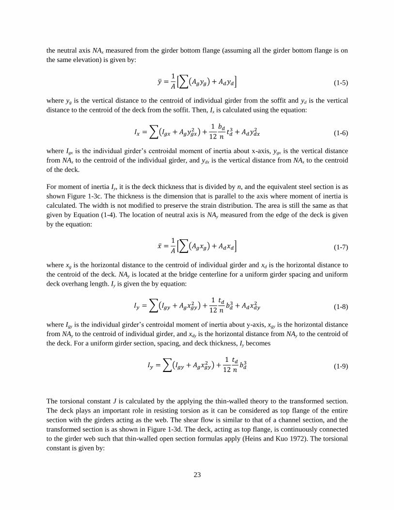
23
the neutral axis NAx measured from the girder bottom flange (assuming all the girder bottom flange is on
the same elevation) is given by:
[∑( ) ] (1-5)
where yg is the vertical distance to the centroid of individual girder from the soffit and yd is the vertical
distance to the centroid of the deck from the soffit. Then, Ix is calculated using the equation:
∑( )
(1-6)
where Igx is the individual girder’s centroidal moment of inertia about x-axis, ygx is the vertical distance
from NAx to the centroid of the individual girder, and ydx is the vertical distance from NAx to the centroid
of the deck.
For moment of inertia Iy, it is the deck thickness that is divided by n, and the equivalent steel section is as
shown Figure 1-3c. The thickness is the dimension that is parallel to the axis where moment of inertia is
calculated. The width is not modified to preserve the strain distribution. The area is still the same as that
given by Equation (1-4). The location of neutral axis is NAy measured from the edge of the deck is given
by the equation:
[∑( ) ] (1-7)
where xg is the horizontal distance to the centroid of individual girder and xd is the horizontal distance to
the centroid of the deck. NAy is located at the bridge centerline for a uniform girder spacing and uniform
deck overhang length. Iy is given the by equation:
∑( )
(1-8)
where Igy is the individual girder’s centroidal moment of inertia about y-axis, xgy is the horizontal distance
from NAy to the centroid of individual girder, and xdy is the horizontal distance from NAy to the centroid of
the deck. For a uniform girder section, spacing, and deck thickness, Iy becomes
∑( )
(1-9)
The torsional constant J is calculated by the applying the thin-walled theory to the transformed section.
The deck plays an important role in resisting torsion as it can be considered as top flange of the entire
section with the girders acting as the web. The shear flow is similar to that of a channel section, and the
transformed section is as shown in Figure 1-3d. The deck, acting as top flange, is continuously connected
to the girder web such that thin-walled open section formulas apply (Heins and Kuo 1972). The torsional
constant is given by:

24
∑
(
)
(1-10)
(1-11)
where h is the is the vertical distance between the center of bottom flange and center of deck as shown in
Figure 1-3d, tw is the web thickness, bbf is the width of the bottom flange, ttf is the thickness of the bottom
flange, Gs is the shear modulus of steel, and Gc is the shear modulus of concrete.
The spine beam is located at the center-of-gravity of the superstructure. It is then connected to rigid beam
elements using rigid links. These rigid beam elements are located at the center-of-gravity of the deck.
They are then connected to the top chords using rigid links, as shown in Figure 1-4b. This modeling is
due to the top chords being connected to the deck discussed in Sections 1.3.1 and 1.3.2 and shown in
Figure 1-1b and Figure 1-2b. The superstructure vertical and longitudinal forces are transferred to the
bearings through the link elements located along the girder lines above the bearings.
The mass from the dead load of superstructure and future wearing surface (see also Section 1.7) were
distributed to the nodes along the superstructure elements. The magnitude of mass assigned to each node
is proportional to the area tributary to that node.
1.6.3 Cross Frames
For elastic analysis, the cross-frames were modeled using beam elements. The effective axial stiffness of
the single angle members is reduced due to end connection eccentricities. In the model, this was achieved
by modifying the area of the cross frames. The effective area (Ae) is calculated as follows (AASHTO
2012):
(1-12)
where Ag is the gross area of the member, I is the section moment of inertia, and e is the eccentricity of
the connection plate relative to the member centroidal axis. However, the resistance of the member is still
calculated using the gross area.
For nonlinear analysis, the cross-frames were modeled using multi-linear plastic link elements. The force-
displacement relationship of these link elements is shown in Figure 1-5. This relationship is based on the
experiments conducted by Bahrami et al. (2010) and Carden et al. (2005). The expected material
properties were used to calculate the yield and buckling load capacities.
1.6.4 Pier Caps and Columns
The pier cap was modeled using beam elements assigned with gross-section properties. In Set I bridges,
these elements are non-prismatic sections to account for the tapered cap.
For elastic analysis, the R/C columns were modeled using beam elements with effective section
properties. These properties are determined through section analysis. For nonlinear analysis, fiber hinges

25
were assigned to the expected locations of plastic hinges. The material properties assigned to the elements
of these hinges were the expected material properties. Unconfined and confined concrete properties were
also used.
The pin connection between the girder and the pier cap was modeled using link elements. The
translational degrees of freedom of these elements were assigned with high stiffness. The rotational
degrees of freedom were unrestrained (i.e. zero stiffness)
1.6.5 Abutment Backfill Soil
At the abutments, in the longitudinal direction, the joint gap and backfill soil were modeled using a series
of gap link element and multi-linear plastic element, respectively. In the transverse direction, the
abutments were unrestrained.
For elastic analysis, the nonlinear properties of link elements were not used and were instead assigned
with equivalent effective stiffness. This effective stiffness is assigned to the element representing the soil
while the gap link element is assigned with high stiffness with no opening. For nonlinear analysis, the gap
element is assigned with an opening as specified in Section 1.3.
1.7 Design Loads
Only dead (DC), future wearing surface (DW), and earthquake (EQ) loads were considered in these
examples. The DC loads were from the weight of the components. For DW, a uniformly distributed area
load of 35 psf was used on the R/C deck. These loads were distributed to the nodes of the superstructure
elements. The magnitude of loads assigned to each node is proportional to its tributary area.
The bridge was assumed to be located in Los Angeles, California with latitude of 34.052 and longitude of
-118.244. The peak ground acceleration (PGA) is 0.671 g, short-period spectral acceleration (Ss) of 1.584
g, and long-period spectral acceleration (S1) of 0.534 g. The bridge was assumed to be founded on a Site
Class B soil thus all the site factors are equal 1.0. The horizontal response acceleration coefficients at 0.2-
second period (SDS) and at 1.0-second period (SD1) are 1.584 g and 0.534 g, respectively. The design
spectrum is shown in Figure 1-6.
The load combination used in the design calculations is Extreme Event I. The load factors are 1.25, 1.5,
and 1.0 for DC, DW, and EQ, respectively. The orthogonal combination of longitudinal and transverse EQ
loads was based on the 100%-30% combination prescribed in AASHTO Specifications.

26
Figure 1-3 Transformed sections used to calculate the equivalent section properties
bbf
bd/n
NAx
Girder
c.g.
ygx1
ydx
ygx2
NAy
td/n
Girder
c.g.
xgy1 xgy2
(a) Steel plate girder composite section
(b) Transformed section for calculation of Ix
(c) Transformed section for calculation of Iy
(d) Thin-walled open section for calculation of J
bbf
ttf
dw
tbf
btf
tw
h
bd
td
td
h
tw
tbf
bd
td/m

27
Figure 1-4 Details of analytical model
(a) 3D view of model
(b) Detail at piers
(c) Detail at abutments
Beam element located at
superstructure c.g.
Columns and pier cap = beam
element
Link element to
transfer superstructure
vertical and
longitudinal forces to
bearings
Cross-frames = beam
elements in elastic
analysis, multi-linear
plastic link elements in
nonlinear analysis.
x
z
y
Rigid beam element located at deck c.g.
Rigid links to connect rigid
beam element to top chord
Gap link element
Soil link element
Link element for
vertical support only
(i.e. free to translate
in any horizontal
direction)

28
Figure 1-5 Force-displacement relationship of ductile cross-frames used for design evaluation
Figure 1-6 Design spectrum
0
0.2
0.4
0.6
0.8
1
1.2
1.4
1.6
1.8
0 1 2 3 4
Acc
eler
atio
n (
g)
Period (sec)

29
1.8 Seismic Evaluation of Design Examples
The seismic performance of bridges designed according to Type 1 and 2 strategies were evaluated
through nonlinear response history analysis.
1.8.1 Ground Motions
The PEER Ground Motion Database (PEER 2013) was used to select historical ground motions that
closely match the design spectrum. The ground motions were selected based on the mean squared error
(MSE) of the difference between the design spectrum and spectral accelerations of records. The seven
ground motions with the lowest MSE were recorded from:
o 1979 Imperial Valley Earthquake at Calexico Fire Station (NGA #162)
o 1983 Coalinga Earthquake at Parkfield – Stone Corral Station (NGA #357)
o 1986 Chalfant Valley Earthquake at Convict Creek station (NGA #551)
o 2003 Big Bear City Earthquake at San Bernardino – Co Service Bldg Station (NGA #2137)
o 1999 Chi-chi Earthquake at CHY039 Station (NGA #2951)
o 1999 Chi-chi Earthquake at CHY088 Station (NGA #2982)
o 1999 Chi-chi Earthquake at TCU075 Station (NGA #3471)
The components of these records were resolved into fault normal (FN) and fault parallel (FP)
components. Table 1-3 shows the scale factors applied to each ground motion that minimizes the MSE
between the design spectrum and geometric mean of the spectra for these components. Figure 1-7 shows
the geometric mean of all spectra from selected records plotted against the design spectrum. The spectra
from the FN and FP components of each record, along with their geometric mean spectrum (GM), plotted
against the design spectrum are shown in Figure 1-8. The FP components were applied in the longitudinal
direction while the FN components were applied in the transverse direction.
These ground motions were also used to analyze the design examples for earthquake levels equivalent to
the Maximum Considered Earthquake (MCE). The MCE is defined by PGA of 0.873 g, Ss of 2.182 g, and
S1 of 0.733 g. Since the spectral accelerations given in AASHTO Specifications are based on design
earthquake, the MCE values were determined from ASCE 7-10 (ASCE 2010). Figure 1-9 shows the MCE
spectrum compared against the response spectra of selected ground motions. Figure 1-10 shows the GM
of the spectra of the seven records plotted against the MCE spectrum.
Seven analyses were performed for the design earthquake and seven analyses were performed for the
MCE earthquake. These analyses are summarized in Table 1-3.

30
Table 1-3 Summary of nonlinear analyses runs
EQ Level Designation Ground Motion
NGA #
Ground Motion Component
Scale Factor Longitudinal
Direction
Transverse
Direction
DE
DE1 162 FP FN 2.79
DE2 357 FP FN 6.14
DE3 551 FP FN 10.73
DE4 2137 FP FN 49.41
DE5 2951 FP FN 9.02
DE6 2982 FP FN 7.02
DE7 3471 FP FN 8.36
MCE
MCE1 162 FP FN 3.83
MCE2 357 FP FN 8.44
MCE3 551 FP FN 14.75
MCE4 2137 FP FN 67.91
MCE5 2951 FP FN 12.40
MCE6 2982 FP FN 9.65
MCE7 3471 FP FN 11.50
Figure 1-7. Comparison of design spectrum and geometric mean of spectra of selected records
0
0.2
0.4
0.6
0.8
1
1.2
1.4
1.6
1.8
2
2.2
2.4
0 0.2 0.4 0.6 0.8 1 1.2 1.4 1.6 1.8 2 2.2 2.4 2.6 2.8 3
Acc
ele
rati
on
(g)
Period (sec)
Design vs GM Spectra of 7 records
GM of 7 records
Design

31
Figure 1-8 Response spectra of selected ground motions compared against design spectrum
0
0.2
0.4
0.6
0.8
1
1.2
1.4
1.6
1.8
2
2.2
2.4
2.6
0 0.2 0.4 0.6 0.8 1 1.2 1.4 1.6 1.8 2
Acc
ele
rati
on
(g)
Period (sec)
Imperial Valley-06 1979 Calexico Fire Station
GM 162
FN 162
FP 162
Design
00.20.40.60.8
11.21.41.61.8
22.22.42.62.8
0 0.2 0.4 0.6 0.8 1 1.2 1.4 1.6 1.8 2
Acc
ele
rati
on
(g)
Period (sec)
Coalinga-01 1983 Parkfield - Stone Corral 3E
GM 357
FN 357
FP 357
Design
0
0.2
0.4
0.6
0.8
1
1.2
1.4
1.6
1.8
2
2.2
0 0.2 0.4 0.6 0.8 1 1.2 1.4 1.6 1.8 2
Acc
ele
rati
on
(g)
Period (sec)
Chalfant Valley-02 1986 Convict Creek
GM 551
FN 551
FP 551
Design
0
0.2
0.4
0.6
0.8
1
1.2
1.4
1.6
1.8
2
2.2
2.4
0 0.2 0.4 0.6 0.8 1 1.2 1.4 1.6 1.8 2
Acc
ele
rati
on
(g)
Period (sec)
Big Bear City 2003 San Bernardino - Co Service Bldg - Freefield
GM 2137
FN 2137
FP 2137
Design
0
0.2
0.4
0.6
0.8
1
1.2
1.4
1.6
1.8
2
2.2
2.4
0 0.2 0.4 0.6 0.8 1 1.2 1.4 1.6 1.8 2
Acc
ele
rati
on
(g)
Period (sec)
Chi-Chi- Taiwan-05 1999 CHY039
GM 2951
FN 2951
FP 2951
Design
0
0.2
0.4
0.6
0.8
1
1.2
1.4
1.6
1.8
2
2.2
2.4
2.6
0 0.2 0.4 0.6 0.8 1 1.2 1.4 1.6 1.8 2
Acc
ele
rati
on
(g)
Period (sec)
Chi-Chi- Taiwan-05 1999 CHY088
GM 2982
FN 2982
FP 2982
Design
00.20.40.60.8
11.21.41.61.8
22.22.42.62.8
33.23.4
0 0.2 0.4 0.6 0.8 1 1.2 1.4 1.6 1.8 2
Acc
ele
rati
on
(g)
Period (sec)
Chi-Chi- Taiwan-06 1999 TCU075
GM 3471
FN 3471
FP 3471
Design

32
Figure 1-9 Response spectra of selected ground motions compared against MCE
00.20.40.60.8
11.21.41.61.8
22.22.42.62.8
33.23.43.6
0 0.2 0.4 0.6 0.8 1 1.2 1.4 1.6 1.8 2
Acc
ele
rati
on
(g)
Period (sec)
Imperial Valley-06 1979 Calexico Fire Station
GM 162
FN 162
FP 162
Design
00.20.40.60.8
11.21.41.61.8
22.22.42.62.8
33.23.43.6
0 0.2 0.4 0.6 0.8 1 1.2 1.4 1.6 1.8 2
Acc
ele
rati
on
(g)
Period (sec)
Coalinga-01 1983 Parkfield - Stone Corral 3E
GM 357
FN 357
FP 357
Design
00.20.40.60.8
11.21.41.61.8
22.22.42.62.8
3
0 0.2 0.4 0.6 0.8 1 1.2 1.4 1.6 1.8 2
Acc
ele
rati
on
(g)
Period (sec)
Chalfant Valley-02 1986 Convict Creek
GM 551
FN 551
FP 551
Design
00.20.40.60.8
11.21.41.61.8
22.22.42.62.8
33.2
0 0.2 0.4 0.6 0.8 1 1.2 1.4 1.6 1.8 2
Acc
ele
rati
on
(g)
Period (sec)
Big Bear City 2003 San Bernardino - Co Service Bldg - Freefield
GM 2137
FN 2137
FP 2137
Design
00.20.40.60.8
11.21.41.61.8
22.22.42.62.8
33.23.4
0 0.2 0.4 0.6 0.8 1 1.2 1.4 1.6 1.8 2
Acc
ele
rati
on
(g)
Period (sec)
Chi-Chi- Taiwan-05 1999 CHY039
GM 2951
FN 2951
FP 2951
Design
00.20.40.60.8
11.21.41.61.8
22.22.42.62.8
33.23.43.6
0 0.2 0.4 0.6 0.8 1 1.2 1.4 1.6 1.8 2
Acc
ele
rati
on
(g)
Period (sec)
Chi-Chi- Taiwan-05 1999 CHY088
GM 2982
FN 2982
FP 2982
Design
00.20.40.60.8
11.21.41.61.8
22.22.42.62.8
33.23.43.63.8
44.24.44.6
0 0.2 0.4 0.6 0.8 1 1.2 1.4 1.6 1.8 2
Acc
ele
rati
on
(g)
Period (sec)
Chi-Chi- Taiwan-06 1999 TCU075
GM 3471
FN 3471
FP 3471
Design

33
Figure 1-10 Comparison of MCE spectrum and geometric mean of spectra of selected records
1.8.2 Calculation of Column Yield Displacement
The ductility demands shown in the nonlinear evaluation of design examples were calculated by dividing
the maximum column displacement by the yield displacement. The maximum column displacement was
obtained from nonlinear analysis. The yield displacement was calculated based on the procedure
discussed below.
1.8.2.1 Single-Column Pier
1.8.2.1.1 Longitudinal Yield Displacement
The longitudinal shear force that creates moment and lateral reaction at the base of the column is applied
to the bearings on top of the pier cap. Since this is at some distance from the top of the column, the
moment created by this shear force to the top of column must be considered in calculating the
displacement at the top of the column. Figure 1-11 shows the schematic diagram of column displacement
and force acting on top of the column. The displacement due to the lateral force P and the moment Pe is
given by the equation:
(1-13)
P is taken as the yield shear force in the column when calculating yield displacement,
0
0.2
0.4
0.6
0.8
1
1.2
1.4
1.6
1.8
2
2.2
2.4
0 0.2 0.4 0.6 0.8 1 1.2 1.4 1.6 1.8 2 2.2 2.4 2.6 2.8 3 3.2 3.4 3.6 3.8 4
Acc
ele
rati
on
(g)
Period (sec)
Design and MCE vs GM Spectra of 7 records
GM of 7 records
MCE Spectrum
Design Spectrum

34
Figure 1-11. Schematic diagram showing the column displacement
1.8.2.1.2 Transverse Direction
Most of the seismic forces are developed in the deck since it comprises more than 80% of the bridge
weight. This seismic force creates overturning in the superstructure which results in vertical reactions in
the bearings, as illustrated in Figure 1-12. These vertical reactions, in turn, create moment at the top of
pier cap. This moment must be added to the moment on top of the column which is created by the shear
force in the bearings. These set of forces is illustrated in Figure 1-12. Since the moment created by the
bearing forces is equal to the overturning moment created by the deck seismic force, the moment at the
top of pier cap is equal to Ph. Equation (1-13) is modified to include this moment in the calculation of
yield displacement:
( )
(1-14)
deck
Bearing
Pier cap
Column H
e
rigid
Δ1 Δ
2
θ
M = Pe
P
Δ1
Top of column
Δ2
θ
Top of bent cap

35
where e is the distance from the top of the column to the centerline of the bearing as shown in Figure
1-11, h is the distance from the centerline of the bearing to the center of gravity of deck. P is taken as the
column yield shear force when calculating the yield displacement.
Figure 1-12. Forces in a single-column pier in the transverse direction.
1.8.2.2 Two-Column Pier
Calculation of the yield displacement in the longitudinal direction is similar to that used in single-column
pier and given by Equation (1-13). In the transverse direction, the pier cap is assumed as rigid and the
displacement at the top of column is calculated using the equation:
(1-15)
where H is the clear height of the column, similar to that shown in Figure 1-11. P is taken as the yield
shear force when calculating the yield displacement. Note that this force is twice the shear force in each
column. This equation is based on double-curvature response in the transverse direction.
1.8.2.3 Wall Pier
The displacement is calculated at the top of the pier. In the longitudinal direction, from the base to top of
wall, is essentially a cantilever column. The displacement is given by:
Pi (-)
P
Po (+)
MT = (P
o - P
i)S
Girder Spacing, S Girder Spacing, S
M = Pe + Ph h

36
(1-16)
where H is the height measured from the base of the wall to the top of wall. In the transverse direction,
the displacement is negligible as it is the strong direction of pier. The displacement is therefore not
evaluated in this direction.
1.8.3 Calculation of Superstructure Drift
The design superstructure drift is calculated using the equation:
(1-17)
where Δlat is the lateral displacement of the superstructure calculated using Eqn. (1-18) and dw is the depth
of girder web. The superstructure lateral displacement is calculated based on the diagonal member
deformation using the equation:
(1-18)
where PEQY is the elastic force in the diagonal member of the cross-frame obtained from response
spectrum analysis in the transverse direction, L is the length, E is its modulus of elasticity, Ae is the
effective area calculated using Eqn. (1-12), and θ is the angle of inclination measured from the horizontal.
Since response spectrum analysis is used in the analysis, the superstructure displacement is not calculated
as the difference between the displacement of the node representing the top of the girder and the
displacement of the node representing the bottom of the girder. This is because the results obtained from
response spectrum analysis are the maximum response after modal combinations. The maximum
displacements in the nodes do not necessarily occur at the same time and, thus, may not be used to obtain
the relative displacement between the top and the bottom of the girder.

37
Chapter 2 Bridge with Single-Column Piers Designed using Type 1
Strategy (Example I-1a)
2.1 Bridge Description
The overall geometry of Ex. I-1a is described in Section 1.3.1. From the final design iteration, the
reinforced concrete (R/C) column diameter is 4 ft with longitudinal and transverse steel ratios of 1.0%.
The pier cap is 5 ft wide, and it is tapered with depth starting from 3 ft-4 in. at the ends to 4 ft at the
center. Figure 2-1 shows the elevation of Ex. I-1a at piers. The cross-frames are of X-type pattern with
diagonal members made of L8x8x5/8 single angles while the top and bottom chords are 2L4x4x1/2
double angles.
2.2 Computational Model
The computational model is shown in Figure 2-2. The equivalent concrete section properties of
superstructure are summarized in Table 2-1. Local axes of the superstructure are shown in Figure 2-1.
Deck cracking was accounted for in the calculation of these properties by using 50% of the gross concrete
modulus of elasticity (Ec).
For nonlinear response history analysis, the cross-frames were modeled with multi-linear plastic link
elements with force-deformation relationship shown in Figure 1-5 to account for inelasticity in case it
occurred. Calculation of expected force and deformations are shown in Section 2.6.
Table 2-1 Ex. I-1a superstructure equivalent concrete section properties
Area, A (in2) 6,028
Moment of inertia about horizontal axis, I2 (in4) 4,660,235
Moment of inertia about vertical axis, I3 (in4) 69,386,665
Torsional constant, J (in4) 102,071

38
Figure 2-1 Elevation at piers of Ex. I-1a
2.3 Analysis
2.3.1 Gravity Loads – DC and DW
The total DC load (i.e. total bridge dead load) is 1,848 kips and the total DW load is 378 kips. The
reactions at the base of column due to these loads are 763 kips and 152 kips, respectively. These loads
were used to calculate the effective section properties of the columns, as illustrated in Section 2.3.2 Steps
1 and 2.
2
3
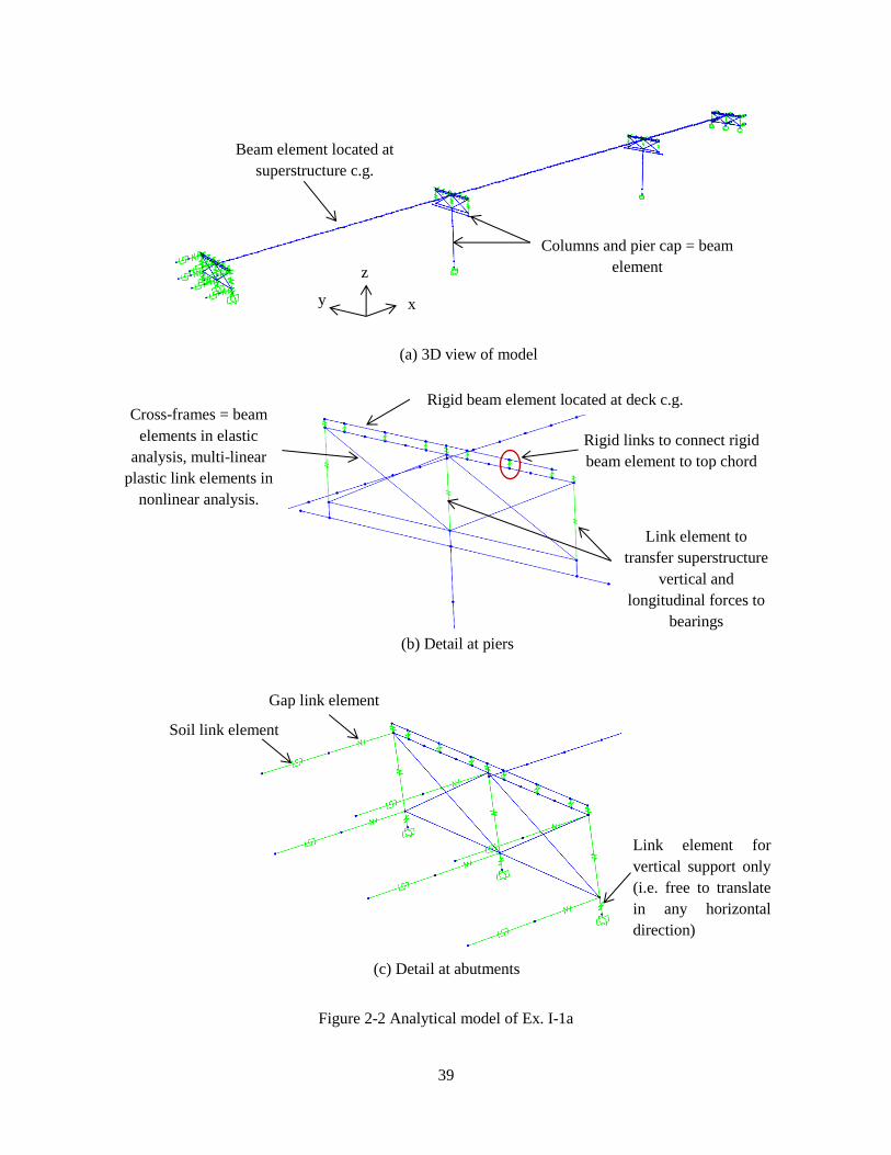
39
Figure 2-2 Analytical model of Ex. I-1a
(a) 3D view of model
(b) Detail at piers
(c) Detail at abutments
Beam element located at
superstructure c.g.
Columns and pier cap = beam
element
Link element to
transfer superstructure
vertical and
longitudinal forces to
bearings
x
z
y
Rigid beam element located at deck c.g.
Rigid links to connect rigid
beam element to top chord
Gap link element
Soil link element
Link element for
vertical support only
(i.e. free to translate
in any horizontal
direction)
Cross-frames = beam
elements in elastic
analysis, multi-linear
plastic link elements in
nonlinear analysis.

40
2.3.2 Earthquake Loads – EQ
Step 1: Calculate column axial loads due to
gravity loads, Pcol.
This will be used to determine the effective
moment of inertia, Ie, of columns.
( ) ( )
Step 2: Determine effective moment of inertia, Ie.
This is accomplished through section analysis of
the column. The required parameters are: column
diameter, longitudinal and transverse
reinforcements, axial load, and material properties
of concrete and steel reinforcement.
The calculated Ie is assigned to the beam elements
representing the column in the model.
The following are the column properties:
D = 4 ft
ρl = 1% (12 - #11)
ρs = 1% (#6 @ 4.0 in.)
f’c = 4 ksi
fy = 60 ksi
Pcol = 1,182 kips
From section analysis:
Ie/Ig = 0.38
Step 3: Estimate soil displacement, Δsoil, and
calculate the effective abutment stiffness, Ke.
The joint gap is included in the calculation of this
stiffness, as shown in the figure below.
Figure 2-3 Abutment force-displacement
The soil passive resistance, Pp, and initial soil
stiffness, Ki, are calculated based on the
recommended values in Caltrans SDC.
( ⁄ ) ( )
( ⁄ ) ( )
where Ae (ft2) is the effective backwall area, h (ft)
is the backwall height, and w is the backwall
Δsoil = 5.01 in.
( )( ⁄ )
( )( ⁄ )
Check Δsoil against Δgap + Δy to determine if the
soil is yielding.
Since this is smaller than Δsoil, the soil is yielding
and the effective stiffness is:

41
width.
Under EQ in longitudinal direction, only one
abutment is engaged in one direction. To account
for this in elastic analyses such as modal and
response spectrum analysis, half of Ke is applied to
both abutments.
This 1/2Ke is then distributed to the link elements
representing the soil. The gap link elements shown
in Figure 2-2c were assigned with high stiffness
with no opening during elastic analysis.
Since there are 6 soil springs at each abutment,
the effective stiffness assigned to each is:
( )
Step 4: Perform modal analysis and determine the
required number of modes needed for multimode
spectral analysis.
After the effective stiffnesses of the elements are
determined, modal analysis is performed to
determine the fundamental vibration periods and
the required number of modes needed in the
response spectrum analysis. The AASHTO
Specifications requires that the total number of
modes used should ensure participation of at least
90% of the total bridge mass.
Table 2-2 shows the result of modal analysis.
Although only the first 5 modes are shown in this
table, a total of 30 modes were used in the
response spectrum analysis with total mass
participation of 100% in both the longitudinal
and transverse directions.
The first mode with period of 2.82 sec is in-plane
deck rotation; the second with period of 2.23 sec
is the transverse translation mode; and the third
with period of 0.92 sec is the longitudinal
translation mode. The vertical vibration mode is
the fourth mode with period of 0.59 sec.
Table 2-2 Modal periods and mass participation
Mode Period Mass Participation
No Sec x-dir y-dir
1 2.82 0.000 0.000
2 2.23 0.000 0.963
3 0.92 0.983 0.000
4 0.59 0.000 0.000
5 0.52 0.000 0.001
Step 5: Perform response spectrum analysis in the
longitudinal direction (EQx), determine Δsoil, and
check against the initial value in Step 3.
The design spectrum is applied in the longitudinal
direction. Multimode spectral analysis is used and
the modal responses are combined using the
Complete Quadratic Combination (CQC).
From response spectrum analysis, Δsoil = 5.01 in.
Therefore, no further iteration is needed.

42
Step 6: Obtain the column forces due to EQx.
These forces will be combined with the forces due
to EQy to determine the design forces.
Table 2-3 Column forces due to EQx
Load P
(kip)
Mx
(k-ft)
My
(k-ft)
EQx 19 0 4,507
The seismic base shear of the bridge in the
longitudinal direction is 1,285 kips.
Step 7: Perform response spectrum analysis in the
transverse direction (EQy) and determine the
column forces.
Table 2-4 Column forces due to EQy
Load P
(kip)
Mx
(k-ft)
My
(k-ft)
EQy 0 7,591 0
The seismic base shear of the bridge in the
transverse direction is 524 kips.

43
2.3.3 Design Loads
The 100%-30% combination was used to combine the EQx and EQy forces. The results are shown in
Table 2-5.
Table 2-5 Combination of forces due to EQx and EQy
Load/Combination P
(kip)
Mx
(k-ft)
My
(k-ft)
EQx 19 0 4,507
EQy 0 7,591 0
EQ1: 1.0EQx + 0.3EQy 19 2,277 4,507
EQ2: 0.3EQx + 1.0EQy 6 7,591 1,352
The response modification factor, R, is then applied to EQ1 and EQ2 column moments. For bridge with
single-column piers, R for columns is equal to 3.0. The resulting forces are then combined with DC and
DW forces to determine the design forces. The load factors are based on Extreme Event I load
combination and the result is shown in Table 2-6.
Table 2-6 Design loads for columns
Load/Combination P
(kip)
Mx
(k-ft)
My
(k-ft)
DC 763 0 0
DW 152 0 0
EQ1/R 19 759 1,502
EQ2/R 6 2,530 451
LC1: 1.25DC + 1.5DW + 1.0EQ1/R 1,201 759 1,502
LC2: 1.25DC + 1.5DW + 1.0EQ2/R 1,188 2,530 451

44
2.4 Design of Columns
Step 1: Determine the design axial load and
resultant moment from Section 2.3.3.
Table 2-7 Design axial load and resultant
moment
Load
Combination
P
(kip)
Mres
(kip-ft)
LC1 1,201 1,683
LC2 1,188 2,570
Step 2: Develop the axial force-moment (P-M)
interaction curve and check if the design loads are
inside the P-M curve.
The AASHTO ϕ factors are used in the interaction
curve.
From the final iteration the column properties
are:
D = 4 ft
ρl = 1% (12 - #11)
ρs = 1% (#6 @ 4.0 in.)
f’c = 4 ksi
fy = 60 ksi
The design loads are within the boundaries of P-
M interaction curve as shown below. Thus, the
selected column size and reinforcement are
adequate.
0
1000
2000
3000
4000
5000
0 500 1000 1500 2000 2500 3000
ϕP
n (
kip
)
ϕMn (kip-ft)

45
Step 3: Determine the plastic shear resistance, Vp,
of the column.
This Vp will be used to design the column
transverse reinforcement and cross-frames. For
single-column piers, Vp is calculated using the
equation:
where Mn is the nominal moment and H is the
height from the base of the column to the
bearings. Mn is determined from interaction curve
based on the axial load, P, in the column. Note
that the ϕ factors are included in the values in the
interaction curve, thus these values are to be
divided by ϕ to get the nominal values. The 1.3
factor is to account for material overstrength.
Using the design axial loads in Table 2-7,
determine the nominal moment from interaction
curve.
for P = 1,201 kips, Mn = 2,977 kip-ft
for P = 1,188 kips Mn = 2,967 kips.
The larger nominal moment is 2,977 kip-ft thus it
will be used to calculate Vp.
( )
Step 4: Determine the column shear resistance and
compare against the plastic shear resistance.
The shear resistance can be calculated using the
Simplified Procedure described in AASHTO
Specifications Art. 5.8.3.4.1. For simplicity and to
be conservative, the contribution of concrete to the
shear resistance is not included in the calculations.
where:
Ash = area of one leg of transverse reinforcement;
fy is the yield stress of transverse reinforcement; s
is the spacing of transverse reinforcement; D is the
diameter of column; Dr is the diameter of the
circle passing through the centers of longitudinal
reinforcement.
The transverse reinforcement is #6 rebar spaced
at 4.0 in. on center. The longitudinal
reinforcement is #11 rebar. The concrete cover is
2.0 in.
( )
( )
( )( )
( )
The demand-resistance ratio is:

46
Step 5: Check the transverse reinforcement.
The volumetric ratio of transverse reinforcement
shall satisfy (AASHTO Specifications Art.
5.10.11.4.1d):
The spacing of transverse reinforcement shall
satisfy (AASHTO Specifications Art.
5.10.11.4.1e):
{
ρs = 1% (#6 @ 4.0 in.)
fy = 60 ksi
f’c = 4 ksi
(
)
{
2.5 Seismic Design of Cross-Frames
For Type 1 design strategy, the inelasticity is to be limited in the columns. The components along the
seismic load path such as cross-frames are designed and detailed to remain elastic.
Step 1: Determine the axial force in each of the
cross-frame diagonal members.
where Vp is the column plastic shear, N is the
number of panels, and θ is the angle of the
diagonal member measured from the horizontal.
Vp = 158 kips
N = 2 panels
θ = 26 degrees
( )( )
Step 2: Cross-frame member section properties
Note that the size of the cross-frames may be
governed by slenderness requirements.
Section: L8x8x5/8
Fy = 36 ksi
Ag = 9.61 in2
rx = 2.48 in.
ry = 2.48 in.
rz = 1.58 in.
L = 149.85 in.

47
Step 3: Calculate the tensile resistance
( )( )
Step 4: Calculate the compressive resistance
Under seismic loading, the cross-frames are
primary members in the transverse direction as
they transmit the deck seismic forces to the
bearings. The limiting slenderness ratio for
primary members is 120 (AASHTO Specifications
Art. 6.9.3).
Equal-leg single angle sections will be used as
diagonal members. The slenderness ratio is
calculated according to AASHTO Specifications
Art. 6.9.4.4.
o If l/rx < 80
(
)
o If l/rx > 80
(
)
where rx is the radius of gyration about the
geometric axis of the angle parallel to the
connected leg.
The compressive resistance is calculated
according to AASHTO Specifications Art. 6.9.2.1,
6.9.4.1.1, and 6.9.4.1.2
( )
The slender element reduction factor, Q, is equal
to 1.0 when:
√
l/rx = 149.85/2.48 = 60.42 < 80
(
)
( )
( )
( )
√
( )( )
[ ]( )

48
o If Pe/Po > 0.44
[ ( ⁄ )]
o If Pe/Po < 0.44
( )
Note that although the calculations shown here is
for equal-leg single angle sections for simplicity,
unequal leg single angles and double angles may
be also used as diagonal members of cross-frames.
The resistance of the selected section, L8x8x5/8,
is much larger than the demand. However, this
section was selected due to limit on slenderness
ratio.
Step 5: Calculate the minimum nominal shear
resistance of the cross-frames and check against
Vp of column.
( )
In this equation, only the nominal compressive
resistance, Pn, is used to determine the minimum
nominal shear resistance. Note that Pn is smaller
than the tensile resistance, Pr, which means
buckling would occur first in any of the diagonal
members before yielding is reached. Thus, VXF is
the minimum nominal shear force before
inelasticity starts to occur in the cross-frames.
Since this is Type 1 design strategy, Vp should be
less than VXF.
(
)
As can be seen above, the slenderness ratio is the
governing parameter in the design of elastic
support cross-frames.

49
2.6 Cross-Frame Properties for Nonlinear Analysis
It is not expected to have inelasticity in the cross-frames using Type I design strategy. However, the
expected force and displacement resistance of the cross-frames are calculated for use in the design
evaluation in case that inelasticity occurred in the analysis.
Step 1: Calculate the expected tensile yield and
displacement resistance.
The expected yield resistance is:
where Fye is the expected yield stress and is equal
to RyFy. For A36 steel sections, Ry = 1.5.
The effective axial stiffness is:
where E is the modulus of elasticity of steel which
is 29,000 ksi, Ae is the effective area calculated
using Eqn. (1-12), and L is the total length of the
diagonal member.
The expected yield displacement is then calculated
as:
L8x4x3/4
Fye = 1.5(36) = 54 ksi
Ag = 9.61 in2
Ix = 59.6 in4
e = 2.21 in. distance from connected leg of angle
to its c.g.
( )
( )
( )
( )

50
Step 2: Calculate the expected compressive
resistance and associated displacement.
The (Kl/r)eff and Pe is the same as that calculated
in Section 2.5 Step 4. The expected yield strength
is used to calculate Po.
The expected compressive resistance is then
calculated as:
o If Pe/Po > 0.44
[ ( ⁄ )]
o If Pe/Po < 0.44
The corresponding displacement is:
( )
( )
51
2.7 Design Summary
The total weight of Ex. I-1a is 1,848 kips. From modal and response spectrum analyses, the periods,
forces, and displacements are:
Parameter Longitudinal Direction Transverse Direction
Fundamental period, T (sec) 0.92 2.23
Base shear, Vb (kip) 1,285 524
Column displacement demand, Δcol (in) 4.60 8.26
Column shear demand, Vcol (in) 184 262
Deck displacement demand, Δdeck (in) 4.92 11.58
The column properties are:
Diameter, D 4 ft
Longitudinal reinforcement 12 - #11 (ρl = 1%)
Transverse reinforcement #6 @ 4.0 in. (ρs = 1%)
Effective moment of inertia, Ie 0.38Ig
Plastic shear resistance, Vp 158 kips
The cross-frame diagonal member section properties are:
Section L8x8x5/8 (A36)
Area, A 9.61 in2
Slenderness ratio, KL/r 117.32
Width-thickness ratio, b/t 12.8
Tensile resistance, ϕPr 329 kips
Compressive resistance, ϕPn 151 kips
Min. nominal shear resistance, VXF_min 603 kips
Expected tensile resistance, Pye 519 kips
Expected compression resistance, Pnc 175 kips

52
2.8 Nonlinear Evaluation
Example I-1a was analyzed using the ground motions described in Section 1.8.1. The ground motions
were scaled to represent the Design (DE) and MCE Earthquake levels. There were seven DE analyses and
seven MCE analyses for a total of fourteen analyses. Because of this, only the column force-displacement
plots from DE1, DE7, MCE1 and MCE7 are shown in Figure 2-4 and Figure 2-5 to represent the results.
However, the column ductility ratios for all runs are shown in Figure 2-6. Nonlinearity was not observed
in the support cross-frames.
The yield displacements were calculated according to Section 1.8.2. Since the expected material
properties were used in the nonlinear analyses, the yield displacements were also calculated using these
properties. The yield displacements are 2.02 in. and 2.15 in. in the longitudinal and transverse directions,
respectively.
In the longitudinal direction, the average ductility ratios were 1.5 from DE runs and 1.9 from MCE runs.
In the transverse direction, the respective ductility ratios were 2.4 and 3.1. The soil resistance at the
abutment reduced the column ductility demand in the longitudinal direction resulting in essentially elastic
response in this direction. The ductility demand in the longitudinal direction is also lower compared to
that in transverse direction because the minor component of the ground motions is applied in this
direction. The ductility demand in the transverse direction clearly indicates yielding of the column, and
the demand in this direction is higher because only the column resists the seismic forces and because the
major component of the ground motions is applied in this direction.
The negative stiffness observed in the hysteresis plots was not due to instability in the structure or
computational error in the analysis. Rather, it is attributed to the coupled biaxial response of the column.
This phenomenon was observed when the response is elastic and depends on the frequency content of the
input motion and period of the structure (Monzon et al. 2013b).
In the transverse direction, the average column base shear forces were 125 kips from DE runs and 135
kips from MCE runs. These forces are about the same because of column yielding. The respective average
of total bearing forces in the transverse direction were 126 kips and 128 kips. Thus, for this bridge, the
inertia force in the pier cap was small. The average of resultant shear forces at the base of the column
were 149 kips from DE runs and 159 kips from MCE runs. From Section 2.7, the plastic shear resistance
of the column is 158 kips.

53
Longitudinal Direction Transverse Direction
(a) DE1
(b) DE7
Figure 2-4 Column force-displacement plots from DE runs
Longitudinal Direction Transverse Direction
(a) MCE1
(b) MCE7
Figure 2-5 Column force-displacement plots from MCE runs
-150
-100
-50
0
50
100
150
-3 -2 -1 0 1 2 3
Shea
r Fo
rce
(ki
p)
Displacement (in)
-150
-100
-50
0
50
100
150
-6 -4 -2 0 2 4
Shea
r Fo
rce
(ki
p)
Displacement (in)
-150
-100
-50
0
50
100
150
-4 -2 0 2 4
Shea
r Fo
rce
(ki
p)
Displacement (in)
-150
-100
-50
0
50
100
150
-6 -4 -2 0 2 4 6
Shea
r Fo
rce
(ki
p)
Displacement (in)
-150
-100
-50
0
50
100
150
-4 -2 0 2 4 6
Shea
r Fo
rce
(ki
p)
Displacement (in)
-150
-100
-50
0
50
100
150
-6 -4 -2 0 2 4 6
Shea
r Fo
rce
(ki
p)
Displacement (in)
-150
-100
-50
0
50
100
150
-4 -2 0 2 4
Shea
r Fo
rce
(ki
p)
Displacement (in)
-150
-100
-50
0
50
100
150
-10 -5 0 5 10
Shea
r Fo
rce
(ki
p)
Displacement (in)

54
(a) ductility ratios in the longitudinal direction
(b) ductility ratios in the transverse direction
Figure 2-6 Summary of column Displacement ductility
0.0
0.5
1.0
1.5
2.0
2.5
3.0
3.5
Dis
pla
cem
en
t D
uct
ility
Ground Motion
Ex. I-1a Column Displacement Ductility: Longitudinal Dir.
0.0
0.5
1.0
1.5
2.0
2.5
3.0
3.5
4.0
4.5
Dis
pla
cem
en
t D
uct
ility
Ground Motion
Ex. I-1a Column Displacement Ductility: Transverse Dir.

55
Chapter 3 Critical Bridge with Single-Column Piers Designed using Type
1 Strategy (Example I-1b)
3.1 Bridge Description
The overall geometry of Ex. I-1b is described in Section 1.3.1. From the final design iteration, the
reinforced concrete (R/C) column diameter is 6.5 ft with longitudinal and transverse steel ratios of 2.4%
and 1.1%. The pier cap is 7 ft wide, and it is tapered with depth starting from 3 ft-4 in. at the ends to 5 ft
at the center. Figure 3-1 shows the elevation of Ex. I-1b at piers. The cross-frames are of X-type pattern
with diagonal members made of WT7x34 while the top and bottom chords are 2L4x4x1/2 double angles.
3.2 Computational Model
The computational model is shown in Figure 3-2. The equivalent concrete section properties of
superstructure are summarized in Table 3-1. Local axes of the superstructure are shown in Figure 3-1.
Deck cracking was accounted for in the calculation of these properties by using 54% of the gross concrete
modulus of elasticity (Ec).
For nonlinear response history analysis, the cross-frames were modeled with multi-linear plastic link
elements with force-deformation relationship shown in Figure 1-5 to account for inelasticity in case it
occurred. Calculation of expected force and deformations are shown in Section 3.6.
Table 3-1 Ex. I-1b superstructure equivalent concrete section properties
Area, A (in2) 6,028
Moment of inertia about horizontal axis, I2 (in4) 4,660,235
Moment of inertia about vertical axis, I3 (in4) 69,386,665
Torsional constant, J (in4) 102,071

56
Figure 3-1 Elevation at piers of Ex. I-1b
3.3 Analysis
3.3.1 Gravity Loads – DC and DW
The total DC load (i.e. total bridge dead load) is 2,076 kips and the total DW load is 378 kips. The
reactions at the base of column due to these loads are 876 kips and 152 kips, respectively. These loads
were used to calculate the effective section properties of the columns, as illustrated in Section 3.3.2 Steps
1 and 2.
2
3

57
Figure 3-2 Analytical model of Ex. I-1b
(a) 3D view of model
(b) Detail at piers
(c) Detail at abutments
Beam element located at
superstructure c.g.
Columns and pier cap = beam
element
Link element to
transfer superstructure
vertical and
longitudinal forces to
bearings
x
z
y
Rigid beam element located at deck c.g.
Rigid links to connect rigid
beam element to top chord
Gap link element
Soil link element
Link element for
vertical support only
(i.e. free to translate
in any horizontal
direction)
Cross-frames = beam
elements in elastic
analysis, multi-linear
plastic link elements in
nonlinear analysis.

58
3.3.2 Earthquake Loads – EQ
Step 1: Calculate column axial loads due to
gravity loads, Pcol.
This will be used to determine the effective
moment of inertia, Ie, of columns.
( ) ( )
Step 2: Determine effective moment of inertia, Ie.
This is accomplished through section analysis of
the column. The required parameters are: column
diameter, longitudinal and transverse
reinforcements, axial load, and material properties
of concrete and steel reinforcement.
The calculated Ie is assigned to the beam elements
representing the column in the model.
The following are the column properties:
D = 6.5 ft
ρl = 2.4% (72 - #11)
ρs = 1.1% (#8 @ 4.0 in.)
f’c = 4 ksi
fy = 60 ksi
Pcol = 1,323 kips
From section analysis:
Ie/Ig = 0.54
Step 3: Estimate soil displacement, Δsoil, and
calculate the effective abutment stiffness, Ke.
The joint gap is included in the calculation of this
stiffness, as shown in the figure below.
Figure 3-3 Abutment force-displacement
The soil passive resistance, Pp, and initial soil
stiffness, Ki, are calculated based on the
recommended values in Caltrans SDC.
( ⁄ ) ( )
( ⁄ ) ( )
where Ae (ft2) is the effective backwall area, h (ft)
is the backwall height, and w is the backwall
Δsoil = 2.8 in.
( )( ⁄ )
( )( ⁄ )
Check Δsoil against Δgap + Δy to determine if the
soil is yielding.
Since this is smaller than Δsoil, the soil is yielding
and the effective stiffness is:

59
width.
Under EQ in longitudinal direction, only one
abutment is engaged in one direction. To account
for this in elastic analyses such as modal and
response spectrum analysis, half of Ke is applied to
both abutments.
This 1/2Ke is then distributed to the link elements
representing the soil. The gap link elements shown
in Figure 3-2c were assigned with high stiffness
with no opening during elastic analysis.
Since there are 6 soil springs at each abutment,
the effective stiffness assigned to each is:
( )
Step 4: Perform modal analysis and determine the
required number of modes needed for multimode
spectral analysis.
After the effective stiffnesses of the elements are
determined, modal analysis is performed to
determine the fundamental vibration periods and
the required number of modes needed in the
response spectrum analysis. The AASHTO
Specifications requires that the total number of
modes used should ensure participation of at least
90% of the total bridge mass.
Table 3-2 shows the result of modal analysis.
Although only the first 5 modes are shown in this
table, a total of 30 modes were used in the
response spectrum analysis with total mass
participation of 100% in both the longitudinal
and transverse directions.
The first mode with period of 1.09 sec is in-plane
deck rotation; the second with period of 0.85 sec
is the transverse translation mode; and the fourth
with period of 0.49 sec is the longitudinal
translation mode. The vertical vibration mode is
the third mode with period of 0.58 sec.
Table 3-2 Modal periods and mass participation
Mode Period Mass Participation
No Sec x-dir y-dir
1 1.09 0.000 0.000
2 0.85 0.000 0.861
3 0.58 0.000 0.000
4 0.49 0.000 0.069
5 0.49 0.956 0.000
Step 5: Perform response spectrum analysis in the
longitudinal direction (EQx), determine Δsoil, and
check against the initial value in Step 3.
The design spectrum is applied in the longitudinal
direction. Multimode spectral analysis is used and
the modal responses are combined using the
Complete Quadratic Combination (CQC).
From response spectrum analysis, Δsoil = 2.78 in.
Therefore, no further iteration is needed.

60
Step 6: Obtain the column forces due to EQx.
These forces will be combined with the forces due
to EQy to determine the design forces.
Table 3-3 Column forces due to EQx
Load P
(kip)
Mx
(k-ft)
My
(k-ft)
EQx 27 0 21,817
The seismic base shear of the bridge in the
longitudinal direction is 2,780 kips.
Step 7: Perform response spectrum analysis in the
transverse direction (EQy) and determine the
column forces.
Table 3-4 Column forces due to EQy
Load P
(kip)
Mx
(k-ft)
My
(k-ft)
EQy 0 20,766 0
The seismic base shear of the bridge in the
transverse direction is 1,354 kips.

61
3.3.3 Design Loads
The 100%-30% combination was used to combine the EQx and EQy forces. The results are shown in
Table 3-5.
Table 3-5 Combination of forces due to EQx and EQy
Load/Combination P
(kip)
Mx
(k-ft)
My
(k-ft)
EQx 27 0 21,817
EQy 0 20,766 0
EQ1: 1.0EQx + 0.3EQy 27 6,230 21,817
EQ2: 0.3EQx + 1.0EQy 8 20,766 6,545
The response modification factor, R, is then applied to EQ1 and EQ2 column moments. For bridge with
single-column piers and under Critical category, R for columns is equal to 1.5. The resulting forces are
then combined with DC and DW forces to determine the design forces. The load factors are based on
Extreme Event I load combination and the result is shown in Table 3-6.
Table 3-6 Design loads for columns
Load/Combination P
(kip)
Mx
(k-ft)
My
(k-ft)
DC 876 0 0
DW 152 0 0
EQ1/R 27 4,153 14,545
EQ2/R 8 13,844 4,363
LC1: 1.25DC + 1.5DW + 1.0EQ1/R 1,350 4,153 14,545
LC2: 1.25DC + 1.5DW + 1.0EQ2/R 1,331 13,844 4,363

62
3.4 Design of Columns
Step 1: Determine the design axial load and
resultant moment from Section 3.3.3.
Table 3-7 Design axial load and resultant
moment
Load
Combination
P
(kip)
Mres
(kip-ft)
LC1 1,350 15,126
LC2 1,331 14,515
Step 2: Develop the axial force-moment (P-M)
interaction curve and check if the design loads are
inside the P-M curve.
The AASHTO ϕ factors are used in the interaction
curve.
From the final iteration the column properties
are:
D = 6.5 ft
ρl = 2.4% (72 - #11)
ρs = 1.1% (#8 @ 4.0 in.)
f’c = 4 ksi
fy = 60 ksi
The design loads are within the boundaries of P-
M interaction curve as shown below. Thus, the
selected column size and reinforcement are
adequate.
Step 3: Determine the plastic shear resistance, Vp,
of the column.
This Vp will be used to design the column
transverse reinforcement and cross-frames. For
single-column piers, Vp is calculated using the
equation:
where Mn is the nominal moment and H is the
Using the design axial loads in Table 3-7,
determine the nominal moment from interaction
curve.
for P = 1,350 kips, Mn = 18,287 kip-ft
for P = 1,331 kips Mn = 18,261 kips.
The larger nominal moment is 18,287 kip-ft thus
it will be used to calculate Vp.
0
2000
4000
6000
8000
10000
12000
14000
16000
0 3000 6000 9000 12000 15000 18000
ϕP
n (
kip
s)
ϕMn (kip-ft)

63
height from the base of the column to the
bearings. Mn is determined from interaction curve
based on the axial load, P, in the column. Note
that the ϕ factors are included in the values in the
interaction curve, thus these values are to be
divided by ϕ to get the nominal values. The 1.3
factor is to account for material overstrength.
( )
Step 4: Determine the column shear resistance and
compare against the plastic shear resistance.
The shear resistance can be calculated using the
Simplified Procedure described in AASHTO
Specifications Art. 5.8.3.4.1. For simplicity and to
be conservative, the contribution of concrete to the
shear resistance is not included in the calculations.
where:
Ash = area of one leg of transverse reinforcement;
fy is the yield stress of transverse reinforcement; s
is the spacing of transverse reinforcement; D is the
diameter of column; Dr is the diameter of the
circle passing through the centers of longitudinal
reinforcement.
The transverse reinforcement is #8 rebar spaced
at 4.0 in. on center. The longitudinal
reinforcement is #11 rebar. The concrete cover is
2.0 in.
( )
( )
( )( )
( )
The demand-resistance ratio is:
Step 5: Check the transverse reinforcement.
The volumetric ratio of transverse reinforcement
shall satisfy (AASHTO Specifications Art.
5.10.11.4.1d):
The spacing of transverse reinforcement shall
satisfy (AASHTO Specifications Art.
5.10.11.4.1e):
ρs = 1.1% (#8 @ 4.0 in.)
fy = 60 ksi
f’c = 4 ksi
(
)
{

64
{
3.5 Seismic Design of Cross-Frames
For Type 1 design strategy, the inelasticity is to be limited in the columns. The components along the
seismic load path such as cross-frames are designed and detailed to remain elastic.
Step 1: Determine the axial force in each of the
cross-frame diagonal members.
where Vp is the column plastic shear, N is the
number of panels, and θ is the angle of the
diagonal member measured from the horizontal.
Vp = 951 kips
N = 2 panels
θ = 26 degrees
( )( )
Step 2: Cross-frame member section properties
Note that the size of the cross-frames may be
governed by slenderness requirements.
Section: WT 7x34
Fy = 50 ksi
Ag = 10 in2
rx = 1.81 in.
Ix = 32.6 in4
e = 1.29 in.
L = 149.85 in.
Step 3: Calculate the tensile resistance
( )( )
Step 4: Calculate the compressive resistance
Under seismic loading, the cross-frames are
primary members in the transverse direction as
they transmit the deck seismic forces to the
bearings. The limiting slenderness ratio for
primary members is 120 (AASHTO Specifications
Art. 6.9.3).
The compressive resistance is calculated
according to AASHTO Specifications Art. 6.9.2.1,
Kl = 1.0(149.85) = 149.85
Kl/r = 149.85/1.81 = 82.79

65
6.9.4.1.1, and 6.9.4.1.2
(
)
The slender element reduction factor, Q, is equal
to 1.0 when:
for flanges:
√
for stem:
√
o If Pe/Po > 0.44
[ ( ⁄ )]
o If Pe/Po < 0.44
( )
( )
( )
√
√
Therefore, Q = 1.0
( )( )
[ ]( )
Step 5: Calculate the minimum nominal shear
resistance of the cross-frames and check against
Vp of column.
( )
In this equation, only the nominal compressive
resistance, Pn, is used to determine the minimum
nominal shear resistance. Note that Pn is smaller
than the tensile resistance, Pr, which means
buckling would occur first in any of the diagonal
members before yielding is reached. Thus, VXF is
the minimum nominal shear force before
inelasticity starts to occur in the cross-frames.
Since this is Type 1 design strategy, Vp should be
less than VXF.
(
)

66
3.6 Cross-Frame Properties for Nonlinear Analysis
It is not expected to have inelasticity in the cross-frames using Type I design strategy. However, the
expected force and displacement resistance of the cross-frames are calculated for use in the design
evaluation in case that inelasticity occurred in the analysis.
Step 1: Calculate the expected tensile yield and
displacement resistance.
The expected yield resistance is:
where Fye is the expected yield stress and is equal
to RyFy. For WT section with A992 Gr 50, Ry =
1.1.
The effective axial stiffness is:
where E is the modulus of elasticity of steel which
is 29,000 ksi, Ae is the effective area calculated
using Eqn. (1-12), and L is the total length of the
diagonal member.
The expected yield displacement is then calculated
as:
L8x4x3/4
Fye = 1.1(50) = 55 ksi
Ag = 10 in2
Ix = 32.6 in4
e = 1.29 in. distance from connected flange of
WT to its c.g.
( )
( )
( )
( )

67
Step 2: Calculate the expected compressive
resistance and associated displacement.
The Kl/r and Pe are the same as that calculated in
Section 3.5 Step 4. The expected yield strength is
used to calculate Po.
The expected compressive resistance is then
calculated as:
o If Pe/Po > 0.44
[ ( ⁄ )]
o If Pe/Po < 0.44
The corresponding displacement is:
( )
[ ]( )

68
3.7 Design Summary
The total weight of Ex. I-1b is 2,076 kips. From modal and response spectrum analyses, the periods,
forces, and displacements are:
Parameter Longitudinal Direction Transverse Direction
Fundamental period, T (sec) 0.49 0.58
Base shear, Vb (kip) 2,780 1,354
Column displacement demand, Δcol (in) 1.85 1.84
Column shear demand, Vcol (in) 853 677
Deck displacement demand, Δdeck (in) 2.8 3.2
The column properties are:
Diameter, D 6.5 ft
Longitudinal reinforcement 72 - #11 (ρl = 2.4%)
Transverse reinforcement #8 @ 4.0 in. (ρs = 1.1%)
Effective moment of inertia, Ie 0.54Ig
Plastic shear resistance, Vp 951 kips
The cross-frame diagonal member section properties are:
Section WT7x34
Area, A 10 in2
Tensile resistance, ϕPr 450 kips
Compressive resistance, ϕPn 303 kips
Min. nominal shear resistance, VXF_min 1,210 kips
Expected tensile resistance, Pye 550 kips
Expected compression resistance, Pnc 317 kips

69
3.8 Nonlinear Evaluation
Example I-1b was analyzed using the ground motions described in Section 1.8.1. The ground motions
were scaled to represent the Design (DE) and MCE Earthquake levels. There were seven DE analyses and
seven MCE analyses for a total of fourteen analyses. Because of this, only the column force-displacement
plots from DE1, DE7, MCE1 and MCE7 are shown in Figure 3-4 and Figure 3-5 to represent the results.
However, the column ductility ratios for all runs are shown in Figure 3-6. Nonlinearity was not observed
in the support cross-frames.
The yield displacements were calculated according to Section 1.8.2. Since the expected material
properties were used in the nonlinear analyses, the yield displacements were also calculated using these
properties. The yield displacements are 1.15 in. and 1.22 in. in the longitudinal and transverse directions,
respectively.
In the longitudinal direction, the average ductility ratios were 1.5 from DE runs and 1.8 from MCE runs.
In the transverse direction, the respective ductility ratios were 1.6 and 2.1. The ductility ratios are smaller
compared to those in Ex. I-1a because the columns in Ex. I-1b are designed for an R-factor of 1.5.
In the transverse direction, the average column base shear forces were 634 kips from DE runs and 705
kips from MCE runs. The respective average of total bearing forces in the transverse direction were 576
kips and 641 kips. Thus, for this bridge, the inertia force in the pier cap is about 10% of the column base
shear. The average of resultant shear forces at the base of the column were 819 kips from DE runs and
906 kips from MCE runs. From Section 3.7, the plastic shear resistance of the column is 951 kips.

70
Longitudinal Direction Transverse Direction
(a) DE1
(b) DE7
Figure 3-4 Column force-displacement plots from DE runs
Longitudinal Direction Transverse Direction
(a) MCE1
(b) MCE7
Figure 3-5 Column force-displacement plots from MCE runs
-800
-600
-400
-200
0
200
400
600
800
-2 -1 0 1 2
Shea
r Fo
rce
(ki
p)
Displacement (in)
-800
-600
-400
-200
0
200
400
600
-2 -1 0 1 2 3
Shea
r Fo
rce
(ki
p)
Displacement (in)
-800
-600
-400
-200
0
200
400
600
800
1000
-2 -1 0 1 2
Shea
r Fo
rce
(ki
p)
Displacement (in)
-800
-600
-400
-200
0
200
400
600
800
-3 -2 -1 0 1 2
Shea
r Fo
rce
(ki
p)
Displacement (in)
-800
-600
-400
-200
0
200
400
600
800
1000
-2 -1 0 1 2
Shea
r Fo
rce
(ki
p)
Displacement (in)
-800
-600
-400
-200
0
200
400
600
800
-2 -1 0 1 2 3
Shea
r Fo
rce
(ki
p)
Displacement (in)
-1000
-800
-600
-400
-200
0
200
400
600
800
1000
-3 -2 -1 0 1 2 3
Shea
r Fo
rce
(ki
p)
Displacement (in)
-1000
-800
-600
-400
-200
0
200
400
600
800
-3 -2 -1 0 1 2 3 4
Shea
r Fo
rce
(ki
p)
Displacement (in)

71
(a) ductility ratios in the longitudinal direction
(b) ductility ratios in the transverse direction
Figure 3-6 Summary of column Displacement ductility
0.0
0.5
1.0
1.5
2.0
2.5
Dis
pla
cem
en
t D
uct
ility
Ground Motion
Ex. I-1b Column Displacement Ductility: Longitudinal Dir.
0.0
0.5
1.0
1.5
2.0
2.5
3.0
Dis
pla
cem
en
t D
uct
ility
Ground Motion
Ex. I-1b Column Displacement Ductility: Transverse Dir.

72
Chapter 4 Bridge with Single-Column Piers Designed using Type 2
Strategy (Example I-2)
4.1 Bridge Description
The overall geometry of Ex. I-2 is described in Section 1.3.1. From the final design iteration, the
reinforced concrete (R/C) column diameter is 5 ft-6 in. with 2.5% longitudinal reinforcement and 1%
transverse reinforcement. The pier cap is 6 ft-6 in. wide, and it is tapered with depth starting from 3 ft-4
in. at the ends to 5 ft at the center. Figure 4-1 shows the elevation of at piers. The cross-frames are of X-
type pattern with diagonal members made of L3x3x3/8 single angles while the top and bottom chords are
2L2x2x1/4 double angles.
4.2 Computational Model
The computational model is shown in Figure 4-2. The equivalent concrete section properties of
superstructure are summarized in Table 4-1. Local axes of the superstructure are shown in Figure 4-1.
Deck cracking was accounted for in the calculation of these properties by using 50% of the gross concrete
modulus of elasticity (Ec).
For elastic analysis, only one of the diagonal members of the cross-frames is included in the model as
shown in Figure 4-2b. This is because the cross-frames are designed and detailed to yield and buckle
under the design earthquake. Under transverse loading, in each cross-frame panel, one diagonal is under
tension and the other is in compression. Consequently, the diagonal in compression would buckle and its
stiffness becomes essentially close to zero.
For nonlinear response history analysis, the cross-frames were modeled with multi-linear plastic link
elements with force-deformation relationship shown in Figure 1-5. The two cross-frame diagonal
members are modeled because buckling is accounted for in the definition of link force-deformation
relationship. Calculation of expected force and deformations are shown in Sections 4.5 and 4.6.
Table 4-1 Ex. I-2 superstructure equivalent concrete section properties
Area, A (in2) 6,028
Moment of inertia about horizontal axis, I2 (in4) 4,660,235
Moment of inertia about vertical axis, I3 (in4) 69,386,665
Torsional constant, J (in4) 102,071

73
Figure 4-1 Elevation at piers of Ex. I-2
4.3 Analysis
4.3.1 Gravity Loads – DC and DW
The total DC load (i.e. total bridge dead load) is 2,014 kips and the total DW load is 378 kips. The
reactions at the base of column due to these loads are 846 kips and 152 kips, respectively. These loads
were used to calculate the effective section properties of the columns, as illustrated in Section 4.3.2 Steps
1 and 2.
2
3

74
Figure 4-2 Analytical model of Ex. I-2
(a) 3D view of model
(b) Detail at piers
(c) Detail at abutments
Beam element located at
superstructure c.g.
Columns and pier cap = beam
element
Link element to
transfer
superstructure
vertical and
longitudinal forces
to bearings
x
z
y
Rigid beam element located at deck c.g.
Rigid links to connect rigid
beam element to top chord
Gap link element
Soil link element
Link element for
vertical support only
(i.e. free to translate
in any horizontal
direction)
Cross-frames = beam
elements in elastic
analysis, multi-linear
plastic link elements in
nonlinear analysis.

75
4.3.2 Earthquake Loads – EQ
Step 1: Calculate column axial loads due to
gravity loads, Pcol.
This will be used to determine the effective
moment of inertia, Ie, of columns.
( ) ( )
Step 2: Determine effective moment of inertia, Ie.
This is accomplished through section analysis of
the column. The required parameters are: column
diameter, longitudinal and transverse
reinforcements, axial load, and material properties
of concrete and steel reinforcement.
The calculated Ie is assigned to the beam elements
representing the column in the model.
The following are the column properties:
D = 5.5 ft
ρl = 2.5% (54 - #11)
ρs = 1% (#6 @ 3.0 in.)
f’c = 4 ksi
fy = 60 ksi
Pcol = 1,286 kips
From section analysis:
Ie/Ig = 0.56
Step 3: Estimate soil displacement, Δsoil, and
calculate the effective abutment stiffness, Ke.
The joint gap is included in the calculation of this
stiffness, as shown in the figure below.
Figure 4-3 Abutment force-displacement
The soil passive resistance, Pp, and initial soil
stiffness, Ki, are calculated based on the
recommended values in Caltrans SDC.
( ⁄ ) ( )
( ⁄ ) ( )
where Ae (ft2) is the effective backwall area, h (ft)
is the backwall height, and w is the backwall
Δsoil = 3.15 in.
( )( ⁄ )
( )( ⁄ )
Check Δsoil against Δgap + Δy to determine if the
soil is yielding.
Since this is smaller than Δsoil, the soil is yielding
and the effective stiffness is:

76
width.
Under EQ in longitudinal direction, only one
abutment is engaged in one direction. To account
for this in elastic analyses such as modal and
response spectrum analysis, half of Ke is applied to
both abutments.
This 1/2Ke is then distributed to the link elements
representing the soil. The gap link elements shown
in Figure 4-2c were assigned with high stiffness
with no opening during elastic analysis.
Since there are 6 soil springs at each abutment,
the effective stiffness assigned to each is:
( )
Step 4: Perform modal analysis and determine the
required number of modes needed for multimode
spectral analysis.
After the effective stiffnesses of the elements are
determined, modal analysis is performed to
determine the fundamental vibration periods and
the required number of modes needed in the
response spectrum analysis. The AASHTO
Specifications requires that the total number of
modes used should ensure participation of at least
90% of the total bridge mass.
Table 4-2 shows the result of modal analysis.
Although only the first 5 modes are shown in this
table, a total of 30 modes were used in the
response spectrum analysis with total mass
participation of 100% in both the longitudinal
and transverse directions.
The first mode with period of 1.58 sec is in-plane
deck rotation; the second with period of 1.22 sec
is the transverse translation mode; and the third
with period of 0.58 sec is the longitudinal
translation mode. The vertical vibration mode is
the fourth mode with period of 0.58 sec.
Table 4-2 Modal periods and mass participation
Mode Period Mass Participation
No Sec x-dir y-dir
1 1.58 0.000 0.000
2 1.22 0.000 0.921
3 0.58 0.969 0.000
4 0.58 0.000 0.000
5 0.51 0.000 0.013
Step 5: Perform response spectrum analysis in the
longitudinal direction (EQx), determine Δsoil, and
check against the initial value in Step 3.
The design spectrum is applied in the longitudinal
direction. Multimode spectral analysis is used and
the modal responses are combined using the
Complete Quadratic Combination (CQC).
From response spectrum analysis, Δsoil = 3.13 in.
This is within 5% of the assumed displacement in
Step 3, thus no further iteration is needed.

77
Step 6: Obtain the column forces due to EQx.
These forces will be used to design the columns.
Table 4-3 Column forces due to EQx
Load P
(kip)
Mx
(k-ft)
My
(k-ft)
EQx 21 0 13,039
The seismic base shear of the bridge in the
longitudinal direction is 2,150 kips.
Step 7: Obtain the column forces due to EQy. Table 4-4 Column forces due to EQy
Load P
(kip)
Mx
(k-ft)
My
(k-ft)
EQy 0 14,894 0
The seismic base shear of the bridge in the
longitudinal direction is 973 kips.
4.3.3 Design Loads
A proposed R factor of 1.5 is applied to moments from earthquake analysis. The forces based on Extreme
Event I load combination is shown below.
Table 4-5 Design loads for columns
Load/Combination P
(kip)
Mx
(k-ft)
My
(k-ft)
DC 846 0 0
DW 152 0 0
EQx 21 0 13,039
EQy 0 14,894 0
EQ1: 1.0EQx + 0.3EQy 21 4,468 13,039
EQ2: 0.3EQx + 1.0EQy 6 14,894 3,912
EQ1/R 21 2,979 8,693
EQ2/R 6 9,929 2,608
LC1: 1.25DC + 1.5DW + 1.0EQ1 1,307 2,979 8,693
LC1: 1.25DC + 1.5DW + 1.0EQ2 1,292 9,929 2,608

78
4.4 Design of Columns
Step 1: Determine the design axial load and
resultant moment from Section 4.3.3.
Table 4-6 Design axial load and resultant
moment
Load
Combination
P
(kip)
Mres
(kip-ft)
LC1 1,307 9,189
LC2 1,292 10,266
Step 2: Develop the axial force-moment (P-M)
interaction curve and check if the design loads are
inside the P-M curve.
The AASHTO ϕ factors are used in the interaction
curve.
From the final iteration the column properties
are:
D = 5.5 ft
ρl = 2.5% (54 - #11)
ρs = 1% (#6 @ 3.0 in.)
f’c = 4 ksi
fy = 60 ksi
The design loads are within the boundaries of P-
M interaction curve as shown below. Thus, the
selected column size and reinforcement are
adequate.
Step 3: Determine the plastic shear resistance, Vp,
of the column.
This Vp will be used to design the column
transverse reinforcement and cross-frames. For
single-column piers, Vp is calculated using the
equation:
Using the design axial loads in Table 4-6,
determine the nominal moment from interaction
curve.
for P = 1,307 kips, Mn = 11,734 kip-ft
for P = 1,292 kips, Mn = 11,720 kip-ft
This larger nominal moment of 11,734 kip-ft will
be used to calculate Vp.
0
2000
4000
6000
8000
10000
12000
0 2000 4000 6000 8000 10000 12000
ϕP
n (
kip
s)
ϕMn (kip-ft)

79
where Mn is the nominal moment and H is the
height from the base of the column to the
bearings. Mn is determined from interaction curve
based on the axial load, P, in the column. Note
that the ϕ factors are included in the values in the
interaction curve, thus these values are to be
divided by ϕ to get the nominal values. The 1.3
factor is to account for material overstrength.
( )
Step 4: Determine the column shear resistance and
compare against the plastic shear resistance.
The shear resistance can be calculated using the
Simplified Procedure described in AASHTO
Specifications Art. 5.8.3.4.1. For simplicity and to
be conservative, the contribution of concrete to the
shear resistance is not included in the calculations.
where:
Ash = area of one leg of transverse reinforcement;
fy is the yield stress of transverse reinforcement; s
is the spacing of transverse reinforcement; D is the
diameter of column; Dr is the diameter of the
circle passing through the centers of longitudinal
reinforcement.
The transverse reinforcement is #6 rebar spaced
at 3.0 in. on center. The longitudinal
reinforcement is #11 rebar. The concrete cover is
2.0 in.
( )
( )
( )( )
( )
The demand-resistance ratio is:
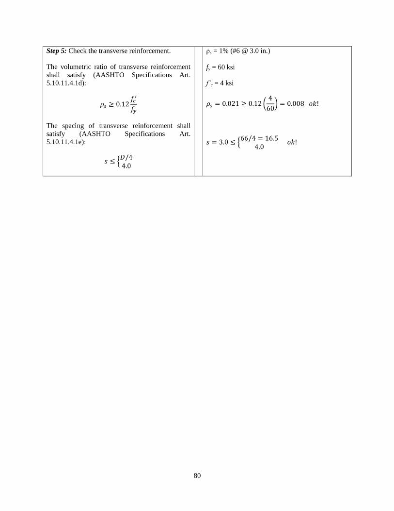
80
Step 5: Check the transverse reinforcement.
The volumetric ratio of transverse reinforcement
shall satisfy (AASHTO Specifications Art.
5.10.11.4.1d):
The spacing of transverse reinforcement shall
satisfy (AASHTO Specifications Art.
5.10.11.4.1e):
{
ρs = 1% (#6 @ 3.0 in.)
fy = 60 ksi
f’c = 4 ksi
(
)
{

81
4.5 Design of Ductile End Cross-Frames
In the proposed Type 2 seismic design, the cross-frames are designed such that their resistance is less than
the column nominal shear resistance in the transverse direction so the inelasticity will be limited to the
cross-frames in that direction.
Step 1: Determine cross-frame force based on
nominal shear resistance of the column.
The cross-frame shear force is equal to nominal
shear resistance of column in the transverse
direction.
where Vp is the column plastic shear resistance.
The corresponding cross-frame diagonal member
axial force with R factor applied is:
where N is the number of panels, θ is the angle of
the diagonal from the horizontal, and R is the
cross-frame modification factor and is equal to
4.0. In this equation, only one diagonal is assumed
resisting the shear force. This is because, in a
panel, one diagonal is in tension and the other one
is in compression. The compression diagonal is
expected to buckle in which case its post-buckling
resistance is considerably smaller, thus the
resistance is largely due to the yield resistance of
the diagonal in tension.
Vp = 600 kips
N = 2
θ = 26o
( )
Step 2: Determine the cross-frame force from
response spectrum analysis in the transverse
direction.
Step 3: The design cross-frame force is the
smaller of PXF1 or PXF2.
PXF = 62 kips
Step 4: Determine cross-frame size. A36 single angle

82
The required area is:
where Fy is the nominal yield stress of the cross-
frame. The nominal value is used since PXF was
calculated from nominal shear force.
Note that the size of the cross-frame may be
governed by the compactness and slenderness
requirements shown in Step 5.
Fy = 36 ksi
Use L3x3x3/8
Ag = 2.11 in2
rz = 0.581 in
I = 1.75 in4
x = 0.884 in. distance from connected leg of
angle to its c.g.
L = 149.85 in
Step 5: Check the compactness and slenderness
ratios.
The diagonal members of ductile cross-frames
shall satisfy (proposed AASHTO Specifications
Art. 6.16.4.5.2a):
√
The slenderness ratio shall satisfy (proposed
AASHTO Specifications Art. 6.16.4.5.2b):
√
where K is 0.85, l is taken as one-half of the
length of the diagonal member due to biased
buckling, r is the radius of gyration normal to the
plane of buckling and is equal to rz for single
angle members.
√
( )
√
Step 6: Calculate the expected yield resistance.
where Fye is the expected yield stress and is equal
to RyFy. For A36 steel sections, Ry = 1.5.
Fye = 1.5(36) = 54 ksi
( )( )
Step 7: Calculate the expected compressive

83
resistance.
The compressive resistance is calculated
according to AASHTO Specifications Art. 6.9.2.1,
6.9.4.1.1, and 6.9.4.1.2
(
)
o If Pe/Po > 0.44
[ ( ⁄ )]
o If Pe/Po < 0.44
( )
( ) ( )
( )
[ ( )]( )
Step 8: Calculate the maximum expected lateral
resistance of the cross-frames and compare against
the column nominal shear resistance.
The maximum lateral resistance is the maximum
of:
( )
where Pt = 1.2Pye is the tensile resistance of the
diagonal member. The 1.5 factor is to account for
the upper bound of tensile resistance. The 0.3Pnc is
the post-buckling resistance of the diagonal
member. Vlat1 typically governs particularly with
relatively slender diagonal members. Vlat2 may
govern in cases when the diagonal members are
short and stocky.
The cross-frame maximum lateral resistance is
compared against the column nominal shear
resistance to ensure elastic columns.
( )
[ ( )]
[ ( )]
Therefore, Vlat = 270 kips
Step 9: Determine the superstructure drift and
check against limit.
After the cross-frame designed, the superstructure
drift is determined. The superstructure lateral
displacement is calculated using the equation:
( )
( )

84
where, PEQY is the force in the cross-frame
diagonal member determined from response
spectrum analysis in the transverse direction and
Ae is the effective area calculated using Eqn.
(1-12).
The superstructure lateral drift should not exceed
4% (proposed AASHTO Specification Art.
6.16.4.5.1).
( )
( )
4.6 Cross-Frame Properties for Nonlinear Analysis
The expected force and displacement resistance of the cross-frames are calculated for use in the design
evaluation.
Step 1: Calculate the expected tensile yield
displacement.
The expected yield resistance is calculated in
Section 4.5 Step 6.
The effective axial stiffness is:
where E is the modulus of elasticity of steel which
is 29,000 ksi, Ae is the effective area calculated
using Eqn. (1-12), and L is the total length of the
diagonal member.
The expected yield displacement is then calculated
as:
L3x3x3/8
Pye = 113.94 kips
Ag = 2.11 in2
I = 1.75 in4
x = 0.884 in. distance from connected leg of
angle to its c.g.
( )
( )
( )
Step 2: Calculate the expected compressive
displacement.
The expected compressive resistance is calculated
in Section 4.5 Step 7.
Pnc = 44.11 kips

85
The corresponding displacement is:
4.7 Design Summary
The total weight of Ex. I-2 is 2,014 kips. From modal and response spectrum analyses, the periods, forces,
and displacements are:
Parameter Longitudinal Direction Transverse Direction
Fundamental period, T (sec) 0.58 1.22
Base shear, Vb (kip) 2,150 973
Column displacement demand, Δcol (in) 2.11 2.48
Column shear demand, Vcol (in) 522 487
Deck displacement demand, Δdeck (in) 3.18 5.78
The column properties are:
Diameter, D 5.5 ft
Longitudinal reinforcement 54 - #11 (ρl = 2.5%)
Transverse reinforcement #6 @ 3.0 in. (ρs = 1%)
Effective moment of inertia, Ie 0.56Ig
Plastic shear resistance, Vp 600 kips
The cross-frame diagonal member section properties are:
Section L3x3x3/8 (A36)
Area, Ag 2.11 in2
Slenderness ratio, KL/r 109.61
Width-thickness ratio, b/t 8.0
Expected tensile yield resistance, Pye 114 kips
Expected compressive resistance, Pnc 44 kips
Lateral resistance of cross-frames, Vlat 270 kips

86
4.8 Nonlinear Evaluation
Example I-2 was analyzed using the ground motions described in Section 1.8.1. The ground motions were
scaled to represent the Design (DE) and MCE Earthquake levels. There were seven DE runs and seven
MCE runs for a total of fourteen runs. Because of this, only the column force-displacement plots from
DE1, DE7, MCE1 and MCE7 are shown in Figure 4-4 and Figure 4-5 to represent the results. However,
the column ductility ratios for all runs are shown in Figure 4-6.
The yield displacements were calculated according to Section 1.8.2. Since the expected material
properties were used in the nonlinear analyses, the yield displacements were also calculated using these
properties. The yield displacements are 1.42 in. and 1.51 in. in the longitudinal and transverse directions,
respectively.
In the longitudinal direction, the average ductility ratios were 1.5 from DE runs and 1.8 from MCE runs.
In the transverse direction, the respective ductility ratios were 1.0 and 1.2. The longitudinal ductility
ratios are comparable to those from Ex. I-1b while the transverse ductility ratios are lower. The yielding
cross-frames limited the seismic forces transmitted to the column in the transverse.
Figure 4-7 and Figure 4-8 shows the superstructure force-displacement in the transverse direction under
DE1, DE7, MCE1, and MCE7. As shown, there was significant yielding in the support cross-frames. It
can be observed that the transverse shear force in the superstructure is about the same as the column
transverse base shear, with the superstructure shear force slightly less. The average of total bearing forces
in the transverse direction was 257 kips under DE and 274 kips under MCE. From Section 4.7, the lateral
resistance of the cross-frames is 270 kips. The total bearing force under MCE is slightly higher because of
strain hardening in the cross-frames. The average column base shear forces in the transverse directions
were 318 kips under DE and 354 kips under MCE. Thus, for this bridge, the inertia force in the pier cap is
about 20% of the base shear.
The average of resultant column base shear forces were 530 kips under DE and 582 kips under MCE.
From Section 4.7, the plastic shear resistance of the column is 600 kips. Thus, the column response is
essentially elastic.
The average lateral displacement of the superstructure under DE was 2.37 in. (3.6% drift). This is about
two times larger than the displacement calculated from the cross-frame design shown in Section 4.5 Step
9 (the displacement is 1.31 in. and the drift is 2%). This difference is attributed to the larger contribution
of the higher modes to the superstructure transverse response. Although the spectral acceleration of the
selected ground motions are close to the design spectrum at fundamental period in transverse direction
(1.22 sec as shown in Table 4-2), the ground motions have larger spectral accelerations at higher modes,
as can be observed in Figure 1-8.

87
Longitudinal Direction Transverse Direction
(a) DE1
(b) DE7
Figure 4-4 Column force-displacement plots from DE runs
Longitudinal Direction Transverse Direction
(a) MCE1
(b) MCE7
Figure 4-5 Column force-displacement plots from MCE runs
-500
-400
-300
-200
-100
0
100
200
300
400
500
-2 -1 0 1 2
Shea
r Fo
rce
(ki
p)
Displacement (in)
-300
-200
-100
0
100
200
300
400
-2 -1.5 -1 -0.5 0 0.5 1 1.5
Shea
r Fo
rce
(ki
p)
Displacement (in)
-600
-400
-200
0
200
400
600
-3 -2 -1 0 1 2 3
Shea
r Fo
rce
(ki
p)
Displacement (in)
-500
-400
-300
-200
-100
0
100
200
300
-2 -1 0 1 2
Shea
r Fo
rce
(ki
p)
Displacement (in)
-600
-400
-200
0
200
400
600
-3 -2 -1 0 1 2 3
Shea
r Fo
rce
(ki
p)
Displacement (in)
-300
-200
-100
0
100
200
300
400
-2 -1 0 1 2
Shea
r Fo
rce
(ki
p)
Displacement (in)
-600
-400
-200
0
200
400
600
800
-4 -3 -2 -1 0 1 2 3
Shea
r Fo
rce
(ki
p)
Displacement (in)
-400
-300
-200
-100
0
100
200
300
400
-2 -1 0 1 2
Shea
r Fo
rce
(ki
p)
Displacement (in)

88
(a) ductility ratios in the longitudinal direction
(b) ductility ratios in the transverse direction
Figure 4-6 Summary of column Displacement ductility
0.0
0.5
1.0
1.5
2.0
2.5D
isp
lace
me
nt
Du
ctili
ty
Ground Motion
Ex. I-2 Column Displacement Ductility: Longitudinal Dir.
0.0
0.2
0.4
0.6
0.8
1.0
1.2
1.4
1.6
1.8
Dis
pla
cem
en
t D
uct
ility
Ground Motion
Ex. I-2 Column Displacement Ductility: Transverse Dir.

89
(a) DE1 (b) DE7
Figure 4-7 Superstructure force-displacement in the transverse direction from DE runs
(a) MCE1 (b) MCE7
Figure 4-8 Superstructure force-displacement in the transverse direction from MCE runs
-300
-200
-100
0
100
200
300
-2.5 -2 -1.5 -1 -0.5 0 0.5
She
ar F
orc
e (
kip
)
Displacement (in)
-300
-200
-100
0
100
200
300
400
-2 -1 0 1 2 3 4 5
She
ar F
orc
e (
kip
)
Displacement (in)
-300
-200
-100
0
100
200
300
-4 -3 -2 -1 0 1
She
ar F
orc
e (
kip
)
Displacement (in)
-300
-200
-100
0
100
200
300
400
-4 -2 0 2 4 6 8
She
ar F
orc
e (
kip
)
Displacement (in)

90
Chapter 5 Bridge with Two-Column Piers Designed using Type 1
Strategy (Example II-1a)
5.1 Bridge Description
The overall geometry of Ex. II-1a is described in Section 1.3.2. From the final design iteration, the
reinforced concrete (R/C) column diameter is 4 ft with 1% longitudinal steel ratio and 1.4% transverse
steel ratio. The rectangular pier cap is 5 ft wide and 4 ft deep. The pier cap is 60 ft long and the center-to-
center distance between the columns is 40 ft. Figure 5-1 shows the elevation at piers. The cross-frames
are of X-type pattern with diagonal members made of L8x8x5/8 single angles while the top and bottom
chords are 2L4x4x1/2 double angles.
5.2 Computational Model
The computational model is shown in Figure 5-2. The equivalent concrete section properties of
superstructure are summarized in Table 5-1. Local axes of the superstructure are shown in Figure 5-1.
Deck cracking was accounted for in the calculation of these properties by using 50% of the gross concrete
modulus of elasticity (Ec).
For nonlinear response history analysis, the cross-frames were modeled with multi-linear plastic link
element with force-deformation relationship shown in Figure 1-5 to account for inelasticity in case it
occurred. Calculation of expected force and deformations are shown in Section 5.6.
Table 5-1 Ex.II-1a superstructure section properties
Area, A (in2) 16,195
Moment of inertia about horizontal axis, I2 (in4) 10,316,084
Moment of inertia about vertical axis, I3 (in4) 8.22 x 10
8
Torsional constant, J (in4) 285,124

91
Figure 5-1 Elevation at pier of Ex. II-1a
5.3 Analysis
5.3.1 Gravity Loads – DC and DW
The total DC load (i.e. total bridge dead load) is 3,933 kips and the total DW load is 844 kips. The
reactions at the base of each column due to these loads are 801 kips and 166 kips, respectively. These
loads were used to calculate the effective section properties of the columns, as illustrated in Section 5.3.2
Steps 1 and 2.
2
3

92
Figure 5-2 Analytical model of Ex. II-1a
(a) 3D view of model
(b) Detail at piers
(c) Detail at abutments
Beam element located at
superstructure c.g.
Columns and pier cap = beam
element
Link element to
transfer
superstructure
vertical and
longitudinal
forces to bearings
x
z
y
Rigid beam element
located at deck c.g.
Rigid links to connect rigid
beam element to top chord
Gap link element
Soil link element
Link element for
vertical support only
(i.e. free to translate
in any horizontal
direction)
Cross-frames = beam
elements in elastic
analysis, multi-linear
plastic link elements in
nonlinear analysis.

93
5.3.2 Earthquake Loads – EQ
Step 1: Calculate column axial loads due to
gravity loads, Pcol.
This will be used to determine the effective
moment of inertia, Ie, of columns.
( ) ( )
Step 2: Determine effective moment of inertia, Ie.
This is accomplished through section analysis of
the column. The required parameters are: column
diameter, longitudinal and transverse
reinforcements, axial load, and material properties
of concrete and steel reinforcement.
The calculated Ie is assigned to the beam elements
representing the column in the model.
The following are the column properties:
D = 4 ft
ρl = 1% (12 - #11)
ρs = 1.4% (#6 @ 3.0 in.)
f’c = 4 ksi
fy = 60 ksi
Pcol = 1,250 kips
From section analysis:
Ie/Ig = 0.38
Step 3: Estimate soil displacement, Δsoil, and
calculate the effective abutment stiffness, Ke.
The joint gap is included in the calculation of this
stiffness, as shown in the figure below.
Figure 5-3 Abutment force-displacement
The soil passive resistance, Pp, and initial soil
stiffness, Ki, are calculated based on the
recommended values in Caltrans SDC.
( ⁄ ) ( )
( ⁄ ) ( )
where Ae (ft2) is the effective backwall area, h (ft)
is the backwall height, and w is the backwall
Δsoil = 5.0 in.
( )( ⁄ )
( )( ⁄ )
Check Δsoil against Δgap + Δy to determine if the
soil is yielding.
Since this is smaller than Δsoil, the soil is yielding
and the effective stiffness is:

94
width.
Under EQ in longitudinal direction, only one
abutment is engaged in one direction. To account
for this in elastic analyses such as modal and
response spectrum analysis, half of Ke is applied to
both abutments.
This 1/2Ke is then distributed to the link elements
representing the soil. The gap link elements shown
in Figure 5-2c were assigned with high stiffness
with no opening during elastic analysis.
Since there are 12 soil springs at each abutment,
the effective stiffness assigned to each is:
( )
Step 4: Perform modal analysis and determine the
required number of modes needed for multimode
spectral analysis.
After the effective stiffnesses of the elements are
determined, modal analysis is performed to
determine the fundamental vibration periods and
the required number of modes needed in the
response spectrum analysis. The AASHTO
Specifications requires that the total number of
modes used should ensure participation of at least
90% of the total bridge mass.
Table 5-2 shows the result of modal analysis.
Although only the first 5 modes are shown in this
table, a total of 30 modes were used in the
response spectrum analysis with total mass
participation of 100% in both the longitudinal
and transverse directions.
The first mode with period of 0.94 sec is
longitudinal translation mode; the second with
period of 0.94 sec is in-plane deck rotation mode;
and the third with period of 0.68 sec is the
transverse translation mode. The vertical
vibration mode is the fourth mode with period of
0.34 sec.
Table 5-2 Modal periods and mass participation
Mode Period Mass Participation
No Sec x-dir y-dir
1 0.94 0.981 0.000
2 0.92 0.000 0.000
3 0.68 0.000 0.980
4 0.34 0.000 0.000
5 0.24 0.000 0.006
Step 5: Perform response spectrum analysis in the
longitudinal direction (EQx), determine Δsoil, and
check against the initial value in Step 3.
The design spectrum is applied in the longitudinal
direction. Multimode spectral analysis is used and
the modal responses are combined using the
Complete Quadratic Combination (CQC).
From response spectrum analysis, Δsoil = 5.05 in.
Therefore, no further iteration is needed.

95
Step 6: Obtain the column forces due to EQx.
These forces will be combined with the forces due
to EQy to determine the design forces.
Table 5-3 Column forces due to EQx
Load P
(kip)
Mx
(k-ft)
My
(k-ft)
EQx 17 0 5,317
The seismic base shear of the bridge in the
longitudinal direction is 2,676 kips.
Step 7: Perform response spectrum analysis in the
transverse direction (EQy) and determine the
column forces.
Table 5-4 Column forces due to EQy
Load P
(kip)
Mx
(k-ft)
My
(k-ft)
EQy 858 9,369 0
The seismic base shear of the bridge in the
transverse direction is 3,731 kips.

96
5.3.3 Design Loads
The 100%-30% combination was used to combine the EQx and EQy forces. The results are shown in
Table 5-5.
Table 5-5 Combination of forces due to EQx and EQy
Load/Combination P
(kip)
Mx
(k-ft)
My
(k-ft)
EQx 17 0 5,317
EQy 858 9,369 0
EQ1: 1.0EQx + 0.3EQy 274 2,811 5,317
EQ2: 0.3EQx + 1.0EQy 863 9,369 1,595
The response modification factor, R, is then applied to EQ1 and EQ2 moments. For bridge with multi-
column piers, R for columns is equal to 5.0. The resulting forces are then combined with DC and DW
forces to determine the design forces. The load factors are based on Extreme Event I load combination
and the result is shown in Table 5-6.
Table 5-6 Design loads for columns
Load/Combination P
(kip)
Mx
(k-ft)
My
(k-ft)
DC 801 0 0
DW 166 0 0
EQ1/R 274 562 1,063
EQ2/R 863 1,874 319
LC1: 1.25DC + 1.5DW + 1.0EQ1 1,524 562 1,063
LC2: 1.25DC + 1.5DW + 1.0EQ2 2,113 1,874 319

97
5.4 Design of Columns
Step 1: Determine the design axial load and
resultant moment from Section 5.3.3.
Table 5-7 Design axial load and resultant moment
Load
Combination
P
(kip)
Mres
(kip-ft)
LC1 1,524 1,202
LC2 2,113 1,901
Step 2: Develop the axial force-moment (P-M)
interaction curve and check if the design loads are
inside the P-M curve.
The AASHTO ϕ factors are used in the interaction
curve.
From the final iteration the column properties are:
D = 4 ft
ρl = 1% (12 - #11)
ρs = 1.4% (#6 @ 3.0 in.)
f’c = 4 ksi
fy = 60 ksi
The design loads are within the boundaries of P-
M interaction curve as shown below. Thus, the
selected column size and reinforcement are
adequate.
Step 3: Determine the plastic shear resistance, Fp,
of the piers in transverse direction
The plastic moment resistance, Mp, of column is a
function of its axial load. In multi-column pier,
due to frame action, there is variation in column
axial loads resulting in different plastic moment
capacities. Calculation of Fp is therefore an
iterative process. The calculation of Fp is outlined
0
1000
2000
3000
4000
5000
0 1000 2000 3000
ϕP
n (
kip
)
ϕMn (kip-ft)

98
in the procedure below.
Step 3.1: Start the calculation process by using the
column axial load, P, obtained from LC1.
The following procedure, up to Step 3.7, is
repeated to calculate Fp based on P from LC2. The
maximum Fp calculated from LC1 and LC2 will
be used to design the transverse reinforcement and
cross-frames
Step 3.2: Based on this P, determine Mn from the
interaction curve.
Step 3.3: Determine Mp and Vp.
where the 1.3 factor is to account for column
overstrength.
where H is the column clear height. This equation
is based on double-curvature behavior. This
behavior is typically assumed for a multi-column
pier because the cap beam is much stiffer than the
columns.
Step 3.4: Calculate Fp and ΔP.
The following equations are based on the free-
body diagram for a two-column pier shown in
Figure 5-4.
From Table 5-7, P = 1,524 kips.
Since this P was from response spectrum
analysis, both columns of the pier have the same
P.
By interpolating on the points of the interaction
curve, Mn = 3,197 kip-ft for P = 1,524 kips.
Mp = 1.3(3,197) = 4,156 kip-ft
Vp = 2(4,156)/20 = 416 kips

99
Figure 5-4 Forces in a two-column pier
( ) ( )
where L is the distance between the two columns.
Step 3.5: Update the axial load in the columns.
Where P1 is the updated axial load in left column
and Pp is updated axial load in right column.
Step 3.6: Update the Mn, Mp, and Vp in the
columns.
The new plastic moments and shears are
determined using P1 and P2.
Step 3.7: Calculate the new Fp and ΔP and
compare against that in Step 3.4.
Fp = 416 + 416 = 832 kips
( ) ( )
P1 = 1,524 – 208 = 1,315 kips
P2 = 1,524 + 208 = 1,731 kips
For P1 = 1,315 kips
Mn1 = 3,058 kip-ft from interaction curve
Mp1 = 1.3(3,058)= 3,975 kip-ft
Vp1 = 2(3,975)/20 = 398 kips
For P2 = 1,731 kips
Mn2 = 3,324 kip-ft from interaction curve
Mp2 = 1.3(3,324) = 4,321 kip-ft
Vp2 = 2(4,321)/20 = 432 kips
Fp = 398 + 432 = 830 kips
Fp
H
Vp1 Vp2Mp1 Mp1
ΔP ΔP

100
If Fp in this step is within 5% of that in Step 3.4,
further iteration is not necessary. Otherwise,
repeat Steps 3.4 to 3.7.
Step 3.8: Repeat Steps 3.1 to 3.7 using P from
LC2.
Step 3.9: Determine the maximum Fp and the
maximum column plastic shear resistance.
This is the maximum of the results from Steps 3.7
and 3.8. The results will be used to design the
column transverse reinforcement and cross-
frames.
( ) ( )
Since Fp and ΔP are within 5% of previous,
further iteration is not necessary.
The calculations were started using P = 2,113
kips from LC2 in Table 5-7. The results of the
last iteration are:
Mp1 = 4,410 kip-ft
Vp1 = 441 kips
Mp2 = 4,571 kip-ft
Vp = 457 kips
Fp = 868 kips
From the results of Steps 3.7 and 3.8:
Vp = 457 kips (maximum Vp per column)
Fp = 868 kips (maximum Fp for the pier)
Step 4: Determine the column shear resistance
and compare against the plastic shear resistance.
The shear resistance can be calculated using the
Simplified Procedure described in AASHTO
Specifications Art. 5.8.3.4.1. For simplicity and to
be conservative, the contribution of concrete to
the shear resistance is not included in the
calculations.
where:
The transverse reinforcement is #6 rebar spaced
at 3.0 in. on center. The longitudinal
reinforcement is #11 rebar. The concrete cover is
2.0 in.
( )
( )

101
Ash = area of one leg of transverse reinforcement;
fy is the yield stress of transverse reinforcement; s
is the spacing of transverse reinforcement; D is
the diameter of column; Dr is the diameter of the
circle passing through the centers of longitudinal
reinforcement.
( )( )
( )
The maximum Vp = 457 kips per column.
The demand-resistance ratio is:
Step 5: Check the transverse reinforcement.
The volumetric ratio of transverse reinforcement
shall satisfy (AASHTO Specifications Art.
5.10.11.4.1d):
The spacing of transverse reinforcement shall
satisfy (AASHTO Specifications Art.
5.10.11.4.1e):
{
ρs = 1.4% (#6 @ 3.0 in.)
fy = 60 ksi
f’c = 4 ksi
(
)
{

102
5.5 Seismic Design of Cross-Frames
For Type 1 design strategy, the inelasticity is to be limited in the columns. The components along the
seismic load path such as cross-frames are designed and detailed to remain elastic.
Step 1: Determine the axial force in each of the
cross-frame diagonal members.
where Fp is the pier plastic shear resistance, N is
the number of panels, and θ is the angle of the
diagonal member measured from the horizontal.
Fp = 868 kips
N = 5 panels
θ = 22 degrees
( )( )
Step 2: Cross-frame member section properties
Note that the size of the cross-frames may be
governed by slenderness requirements.
Section: L8x8x5/8
Fy = 36 ksi
Ag = 9.61 in2
rx = ry = 2.48 in.
L = 142.62 in.
Step 3: Calculate the tensile resistance
( )( )
Step 4: Calculate the compressive resistance
Under seismic loading, the cross-frames are
primary members in the transverse direction as
they transmit the deck seismic forces to the
bearings. The limiting slenderness ratio for
primary members is 120 (AASHTO Specifications
Art. 6.9.3).
Equal-leg single angle sections will be used as
diagonal members. The slenderness ratio is
calculated according to AASHTO Specifications
Art. 6.9.4.4.
o If l/rx < 80
(
)
o If l/rx > 80
l/rx = 142.62/2.48 = 57.51 < 80
(
)
( )

103
(
)
The compressive resistance is calculated
according to AASHTO Specifications Art. 6.9.2.1,
6.9.4.1.1, and 6.9.4.1.2
(
)
The slender element reduction factor, Q, is equal
to 1.0 when:
√
o If Pe/Po > 0.44
[ ( ⁄ )]
o If Pe/Po < 0.44
( )
Note that although the calculations shown here is
for single angle sections, unequal-leg single
angles and double angles may be also used as
diagonal members of cross-frames.
( )
( )
√
( )( )
[ ]( )
The resistance of the selected section, L8x8x5/8,
is much larger than the demand. However, this
section was selected due to limit on slenderness
ratio.
Step 5: Calculate the minimum nominal shear
resistance of the cross-frames and check against
Vp of column.
( )
In this equation, only the compression resistance,
Pn, is used to determine the minimum nominal
shear resistance. Note that Pn is smaller than the
tension resistance, Pr, which means buckling
would occur first in any of the diagonal members
before yielding is reached. Thus, VXF is the
minimum shear force before inelasticity starts to
occur in the cross-frames. Since this is Type 1
design – inelasticity is accommodated in the
columns only – Fp should be less thanVXF.
(
)
As can be seen above, the slenderness ratio is the
governing parameter in the design of elastic
support cross-frames.

104
5.6 Cross-Frame Properties for Nonlinear Analysis
The expected force and displacement resistance of the cross-frames are calculated for use in the design
evaluation.
Step 1: Calculate the expected tensile yield and
displacement resistance.
The expected yield resistance is:
where Fye is the expected yield stress and is equal
to RyFy. For A36 steel sections, Ry = 1.5.
The effective axial stiffness is:
where E is the modulus of elasticity of steel which
is 29,000 ksi, Ae is the effective area calculated
using Eqn. (1-12), and L is the total length of the
diagonal member.
The expected yield displacement is then calculated
as:
L8x8x5/8
Fye = 1.5(36) = 54 ksi
Ag = 9.61 in2
I = 59.6 in4
e = 2.21 in. distance from connected leg of angle
to its c.g.
( )
( )
( )
( )
Step 2: Calculate the expected compressive
resistance and associated displacement.
The (Kl/r)eff and Pe is the same as that calculated
in Section 5.5 Step 4. The expected yield strength
is used to calculate Po.
The expected compressive resistance is then
calculated as:
o If Pe/Po > 0.44
[ ( ⁄ )]
o If Pe/Po < 0.44
( )
( )

105
The corresponding displacement is:
5.7 Design Summary
The total weight of Ex. II-1a is 3,933 kips. From modal and response spectrum analyses, the periods,
forces, and displacements are:
Parameter Longitudinal Direction Transverse Direction
Fundamental period, T (sec) 0.94 0.68
Base shear, Vb (kip) 2,676 3,731
Column displacement demand, Δcol (in) 3.73 3.17
Column shear demand, Vcol (kip) 225 933
Pier base shear demand, Fb (kip) 450 1,866
Deck displacement demand, Δdeck (in) 5.06 3.37
The column properties are:
Diameter, D 4 ft
Longitudinal reinforcement 12 - #11 (ρl = 1%)
Transverse reinforcement #6 @ 3.0 in. (ρs = 1.4%)
Effective moment of inertia, Ie 0.38Ig
Column plastic shear resistance, Vp 457 kips
Pier plastic shear resistance, Fp 898 kips
The cross-frame diagonal member section properties are:
Section L8x8x5/8 (A36)
Area, A 9.61 in2
Slenderness ratio, KL/r 115.13
Width-thickness ratio, b/t 12.8
Tensile resistance, ϕPr 329 kips
Compressive resistance, ϕPn 155 kips
Min. nominal shear resistance, VXF_min 1,597 kips
Expected tensile yield resistance, Pye 519 kips
Expected compressive resistance, Pnc 182 kips

106
5.8 Nonlinear Evaluation
Example II-1a was analyzed using the ground motions described in Section 1.8.1. The ground motions
were scaled to represent the Design (DE) and MCE Earthquake levels. There were seven DE runs and
seven MCE runs for a total of fourteen runs. Because of this, only the column force-displacement plots
from DE1, DE7, MCE1 and MCE7 are shown in Figure 5-5 and Figure 5-6 to represent the results.
However, the column ductility ratios for all runs are shown in Figure 5-7. Nonlinearity was not observed
in the support cross-frames.
The yield displacements were calculated according to Section 1.8.2. Since the expected material
properties were used in the nonlinear analyses, the yield displacements were also calculated using these
properties. The yield displacements are 1.91 in. and 0.88 in. in the longitudinal and transverse directions,
respectively.
In the longitudinal direction, the average ductility ratios were 1.7 from DE runs and 2.3 from MCE runs.
In the transverse direction, the respective ductility ratios were 3.8 and 5.2. The smaller ductility in the
longitudinal direction is due to the contribution of abutment soil in the response. The column response in
this direction is single-curvature resulting in yield displacement that is about three times the yield
displacement in transverse direction. Thus, the ductility demand in the transverse direction is larger even
though the displacements in both directions are about the same. Yielding is also apparent in the hysteresis
loops in the transverse direction.
The average of total bearing forces in the transverse direction were 902 kips under DE and 1,010 kips
under MCE. These are smaller than the minimum nominal resistance of the cross-frames shown in
Section 5.7 thus the cross-frames were elastic. The average of pier base shear forces in the transverse
direction were 980 kips under DE and 1,091 kips under MCE. Thus, for this bridge, the inertia force in
the pier cap is about 8% of the pier base shear.

107
Longitudinal Direction Transverse Direction
(a) DE1
(b) DE7
Figure 5-5 Column force-displacement plots from DE runs
Longitudinal Direction Transverse Direction
(a) MCE1
(b) MCE7
Figure 5-6 Column force-displacement plots from MCE runs
-300
-200
-100
0
100
200
300
-3 -2 -1 0 1 2 3
Shea
r Fo
rce
, Fx
(kip
)
Displacement, Ux (in)
-1000
-800
-600
-400
-200
0
200
400
600
800
1000
-4 -2 0 2 4
She
ar F
orc
e, F
y (k
ip)
Displacement, Uy (in)
-400
-300
-200
-100
0
100
200
300
400
-4 -2 0 2 4
Shea
r Fo
rce
, Fx
(kip
)
Displacement, Ux (in)
-1500
-1000
-500
0
500
1000
1500
-4 -2 0 2 4Sh
ear
Fo
rce
, Fy
(kip
)
Displacement, Uy (in)
-400
-300
-200
-100
0
100
200
300
400
-4 -2 0 2 4 6
Shea
r Fo
rce
, Fx
(kip
)
Displacement, Ux (in)
-1000
-500
0
500
1000
1500
-6 -4 -2 0 2 4
She
ar F
orc
e, F
y (k
ip)
Displacement, Uy (in)
-400
-300
-200
-100
0
100
200
300
400
-6 -4 -2 0 2 4 6
Shea
r Fo
rce
, Fx
(kip
)
Displacement, Ux (in)
-1500
-1000
-500
0
500
1000
1500
-4 -2 0 2 4 6
She
ar F
orc
e, F
y (k
ip)
Displacement, Uy (in)

108
(a) ductility ratios in the longitudinal direction
(b) ductility ratios in the transverse direction
Figure 5-7 Summary of column Displacement ductility
0.0
0.5
1.0
1.5
2.0
2.5
3.0
3.5
Dis
pla
cem
en
t D
uct
ility
Ground Motion
Ex. II-1a Column Displ. Ductility: Longitudinal Dir.
0.0
1.0
2.0
3.0
4.0
5.0
6.0
7.0
8.0
Dis
pla
cem
en
t D
uct
ility
Ground Motion
Ex. II-1a Column Displ Ductility: Transverse Dir.
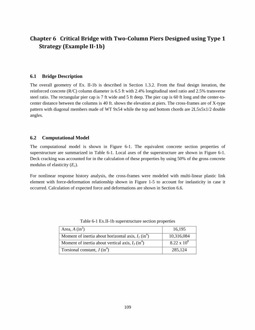
109
Chapter 6 Critical Bridge with Two-Column Piers Designed using Type 1
Strategy (Example II-1b)
6.1 Bridge Description
The overall geometry of Ex. II-1b is described in Section 1.3.2. From the final design iteration, the
reinforced concrete (R/C) column diameter is 6.5 ft with 2.4% longitudinal steel ratio and 2.5% transverse
steel ratio. The rectangular pier cap is 7 ft wide and 5 ft deep. The pier cap is 60 ft long and the center-to-
center distance between the columns is 40 ft. shows the elevation at piers. The cross-frames are of X-type
pattern with diagonal members made of WT 9x54 while the top and bottom chords are 2L5x5x1/2 double
angles.
6.2 Computational Model
The computational model is shown in Figure 6-1. The equivalent concrete section properties of
superstructure are summarized in Table 6-1. Local axes of the superstructure are shown in Figure 6-1.
Deck cracking was accounted for in the calculation of these properties by using 50% of the gross concrete
modulus of elasticity (Ec).
For nonlinear response history analysis, the cross-frames were modeled with multi-linear plastic link
element with force-deformation relationship shown in Figure 1-5 to account for inelasticity in case it
occurred. Calculation of expected force and deformations are shown in Section 6.6.
Table 6-1 Ex.II-1b superstructure section properties
Area, A (in2) 16,195
Moment of inertia about horizontal axis, I2 (in4) 10,316,084
Moment of inertia about vertical axis, I3 (in4) 8.22 x 10
8
Torsional constant, J (in4) 285,124

110
Figure 6-1 Elevation at pier of Ex. II-1b
6.3 Analysis
6.3.1 Gravity Loads – DC and DW
The total DC load (i.e. total bridge dead load) is 4,573 kips and the total DW load is 844 kips. The
reactions at the base of each column due to these loads are 959 kips and 166 kips, respectively. These
loads were used to calculate the effective section properties of the columns, as illustrated in Section 6.3.2
Steps 1 and 2.
2
3

111
Figure 6-2 Analytical model of Ex. II-1b
(a) 3D view of model
(b) Detail at piers
(c) Detail at abutments
Beam element located at
superstructure c.g.
Columns and pier cap = beam
element
Link element to
transfer
superstructure
vertical and
longitudinal
forces to bearings
x
z
y
Rigid beam element
located at deck c.g.
Rigid links to connect rigid
beam element to top chord
Gap link element
Soil link element
Link element for
vertical support only
(i.e. free to translate
in any horizontal
direction)
Cross-frames = beam
elements in elastic
analysis, multi-linear
plastic link elements in
nonlinear analysis.

112
6.3.2 Earthquake Loads – EQ
Step 1: Calculate column axial loads due to
gravity loads, Pcol.
This will be used to determine the effective
moment of inertia, Ie, of columns.
( ) ( )
Step 2: Determine effective moment of inertia, Ie.
This is accomplished through section analysis of
the column. The required parameters are: column
diameter, longitudinal and transverse
reinforcements, axial load, and material properties
of concrete and steel reinforcement.
The calculated Ie is assigned to the beam elements
representing the column in the model.
The following are the column properties:
D = 6.5 ft
ρl = 2.4% (72 - #11)
ρs = 2.5% (#8 @ 1.75 in.)
f’c = 4 ksi
fy = 60 ksi
Pcol = 1,448 kips
From section analysis:
Ie/Ig = 0.54
Step 3: Estimate soil displacement, Δsoil, and
calculate the effective abutment stiffness, Ke.
The joint gap is included in the calculation of this
stiffness, as shown in the figure below.
Figure 6-3 Abutment force-displacement
The soil passive resistance, Pp, and initial soil
stiffness, Ki, are calculated based on the
recommended values in Caltrans SDC.
( ⁄ ) ( )
( ⁄ ) ( )
where Ae (ft2) is the effective backwall area, h (ft)
is the backwall height, and w is the backwall
Δsoil = 3.0 in.
( )( ⁄ )
( )( ⁄ )
Check Δsoil against Δgap + Δy to determine if the
soil is yielding.
Since this is smaller than Δsoil, the soil is yielding
and the effective stiffness is:

113
width.
Under EQ in longitudinal direction, only one
abutment is engaged in one direction. To account
for this in elastic analyses such as modal and
response spectrum analysis, half of Ke is applied to
both abutments.
This 1/2Ke is then distributed to the link elements
representing the soil. The gap link elements shown
in Figure 5-2c were assigned with high stiffness
with no opening during elastic analysis.
Since there are 12 soil springs at each abutment,
the effective stiffness assigned to each is:
( )
Step 4: Perform modal analysis and determine the
required number of modes needed for multimode
spectral analysis.
After the effective stiffnesses of the elements are
determined, modal analysis is performed to
determine the fundamental vibration periods and
the required number of modes needed in the
response spectrum analysis. The AASHTO
Specifications requires that the total number of
modes used should ensure participation of at least
90% of the total bridge mass.
Table 6-2 shows the result of modal analysis.
Although only the first 5 modes are shown in this
table, a total of 30 modes were used in the
response spectrum analysis with total mass
participation of 100% in both the longitudinal
and transverse directions.
The second mode with period of 0.57 sec is
longitudinal translation mode; the third with
period of 0.45 sec is in-plane deck rotation mode;
and the fourth with period of 0.35 sec is the
transverse translation mode. The vertical
vibration mode is the first mode with period of
0.57 sec.
Table 6-2 Modal periods and mass participation
Mode Period Mass Participation
No Sec x-dir y-dir
1 0.57 0.000 0.000
2 0.51 0.955 0.000
3 0.45 0.000 0.000
4 0.35 0.000 0.774
5 0.34 0.002 0.000
Step 5: Perform response spectrum analysis in the
longitudinal direction (EQx), determine Δsoil, and
check against the initial value in Step 3.
The design spectrum is applied in the longitudinal
direction. Multimode spectral analysis is used and
the modal responses are combined using the
Complete Quadratic Combination (CQC).
From response spectrum analysis, Δsoil = 2.96 in.
Therefore, no further iteration is needed.

114
Step 6: Obtain the column forces due to EQx.
These forces will be combined with the forces due
to EQy to determine the design forces.
Table 6-3 Column forces due to EQx
Load P
(kip)
Mx
(k-ft)
My
(k-ft)
EQx 36 0 24,766
The seismic base shear of the bridge in the
longitudinal direction is 5,722 kips.
Step 7: Perform response spectrum analysis in the
transverse direction (EQy) and determine the
column forces.
Table 6-4 Column forces due to EQy
Load P
(kip)
Mx
(k-ft)
My
(k-ft)
EQy 1,580 17,777 0
The seismic base shear of the bridge in the
transverse direction is 6,681 kips.

115
6.3.3 Design Loads
The 100%-30% combination was used to combine the EQx and EQy forces. The results are shown in
Table 5-5.
Table 6-5 Combination of forces due to EQx and EQy
Load/Combination P
(kip)
Mx
(k-ft)
My
(k-ft)
EQx 36 0 24,766
EQy 1,580 17,777 0
EQ1: 1.0EQx + 0.3EQy 510 5,331 24,766
EQ2: 0.3EQx + 1.0EQy 1,591 17,777 7,430
The response modification factor, R, is then applied to EQ1 and EQ2 moments. For a critical bridge with
multi-column piers, R for columns is equal to 1.5. The resulting forces are then combined with DC and
DW forces to determine the design forces. The load factors are based on Extreme Event I load
combination and the result is shown in Table 6-6.
Table 6-6 Design loads for columns
Load/Combination P
(kip)
Mx
(k-ft)
My
(k-ft)
DC 959 0 0
DW 166 0 0
EQ1/R 510 3,554 16,511
EQ2/R 1,591 11,851 4,953
LC1: 1.25DC + 1.5DW + 1.0EQ1 1,959 3,554 16,511
LC2: 1.25DC + 1.5DW + 1.0EQ2 3,040 11,851 4,953

116
6.4 Design of Columns
Step 1: Determine the design axial load and
resultant moment from Section 5.3.3.
Table 6-7 Design axial load and resultant moment
Load
Combination
P
(kip)
Mres
(kip-ft)
LC1 1,959 16,889
LC2 3,040 12,844
Step 2: Develop the axial force-moment (P-M)
interaction curve and check if the design loads are
inside the P-M curve.
The AASHTO ϕ factors are used in the interaction
curve.
From the final iteration the column properties are:
D = 6.5 ft
ρl = 2.4% (72 - #11)
ρs = 2.5% (#8 @ 1.75 in.)
f’c = 4 ksi
fy = 60 ksi
The design loads are within the boundaries of P-
M interaction curve as shown below. Thus, the
selected column size and reinforcement are
adequate.
Step 3: Determine the plastic shear resistance, Fp,
of the piers in transverse direction
The plastic moment resistance, Mp, of column is a
function of its axial load. In multi-column pier,
due to frame action, there is variation in column
axial loads resulting in different plastic moment
capacities. Calculation of Fp is therefore an
iterative process. The calculation of Fp is outlined
in the procedure below.
0
2000
4000
6000
8000
10000
12000
14000
16000
0 5000 10000 15000 20000
ϕP
n (
kip
s)
ϕMn (kip-ft)

117
Step 3.1: Start the calculation process by using the
column axial load, P, obtained from LC1.
The following procedure, up to Step 3.7, is
repeated to calculate Fp based on P from LC2. The
maximum Fp calculated from LC1 and LC2 will
be used to design the transverse reinforcement and
cross-frames
Step 3.2: Based on this P, determine Mn from the
interaction curve.
Step 3.3: Determine Mp and Vp.
where the 1.3 factor is to account for column
overstrength.
where H is the column clear height. This equation
is based on double-curvature behavior. This
behavior is typically assumed for a multi-column
pier because the cap beam is much stiffer than the
columns.
Step 3.4: Calculate Fp and ΔP.
The following equations are based on the free-
body diagram for a two-column pier shown in
Figure 6-4.
From Table 6-7, P = 1,959 kips.
Since this P was from response spectrum
analysis, both columns of the pier have the same
P.
By interpolating on the points of the interaction
curve, Mn = 19,006 kip-ft for P = 1,959 kips.
Mp = 1.3(19,006) = 24,708 kip-ft
Vp = 2(24,708)/20 = 2,471 kips

118
Figure 6-4 Forces in a two-column pier
( ) ( )
where L is the distance between the two columns.
Step 3.5: Update the axial load in the columns.
Where P1 is the updated axial load in left column
and Pp is updated axial load in right column.
Step 3.6: Update the Mn, Mp, and Vp in the
columns.
The new plastic moments and shears are
determined using P1 and P2.
Step 3.7: Calculate the new Fp and ΔP and
compare against that in Step 3.4.
Fp = 2,471 + 2,471 = 4,942 kips
( ) ( )
P1 = 1,959 – 1,236 = 723 kips
P2 = 1,959 + 1,236 = 3,195 kips
For P1 = 723 kips
Mn1 = 17,341 kip-ft from interaction
curve
Mp1 = 1.3(17,341)=22,544 kip-ft
Vp1 = 2(22,544)/20 = 2,254 kips
For P2 = 3,195 kips
Mn2 = 19,477 kip-ft from interaction
curve
Mp2 = 1.3(19,477) = 25,320 kip-ft
Vp2 = 2(25,320)/20 = 2,532 kips
Fp = 2,254 + 2,532 = 4,786 kips
Fp
H
Vp1 Vp2Mp1 Mp1
ΔP ΔP

119
If Fp in this step is within 5% of that in Step 3.4,
further iteration is not necessary. Otherwise,
repeat Steps 3.4 to 3.7.
Step 3.8: Repeat Steps 3.1 to 3.7 using P from
LC2.
Step 3.9: Determine the maximum Fp and the
maximum column plastic shear resistance.
This is the maximum of the results from Steps 3.7
and 3.8. The results will be used to design the
column transverse reinforcement and cross-
frames.
( ) ( )
Since Fp and ΔP are within 5% of previous,
further iteration is not necessary.
The calculations were started using P = 3,040
kips from LC2 in Table 6-7. The results of the
last iteration are:
Mp1 = 24,518 kip-ft
Vp1 = 2,452 kips
Mp2 = 24,931 kip-ft
Vp2 = 2,493 kips
Fp = 4,945 kips
From the results of Steps 3.7 and 3.8:
Vp = 2,532 kips (maximum Vp per column)
Fp = 4,945 kips (maximum Fp for the pier)
Step 4: Determine the column shear resistance
and compare against the plastic shear resistance.
The shear resistance can be calculated using the
Simplified Procedure described in AASHTO
Specifications Art. 5.8.3.4.1. For simplicity and to
be conservative, the contribution of concrete to
the shear resistance is not included in the
calculations.
where:
The transverse reinforcement is #8 rebar spaced
at 1.75 in. on center. The longitudinal
reinforcement is #11 rebar. The concrete cover is
2.0 in.
( )
( )

120
Ash = area of one leg of transverse reinforcement;
fy is the yield stress of transverse reinforcement; s
is the spacing of transverse reinforcement; D is
the diameter of column; Dr is the diameter of the
circle passing through the centers of longitudinal
reinforcement.
( )( )
( )
The maximum Vp = 2,532 kips per column.
The demand-resistance ratio is:
Step 5: Check the transverse reinforcement.
The volumetric ratio of transverse reinforcement
shall satisfy (AASHTO Specifications Art.
5.10.11.4.1d):
The spacing of transverse reinforcement shall
satisfy (AASHTO Specifications Art.
5.10.11.4.1e):
{
ρs = 2.5% (#8 @ 1.75 in.)
fy = 60 ksi
f’c = 4 ksi
(
)
{

121
6.5 Seismic Design of Cross-Frames
For Type 1 design strategy, the inelasticity is to be limited in the columns. The components along the
seismic load path such as cross-frames are designed and detailed to remain elastic.
Step 1: Determine the axial force in each of the
cross-frame diagonal members.
where Fp is the pier plastic shear resistance, N is
the number of panels, and θ is the angle of the
diagonal member measured from the horizontal.
Fp = 4,945 kips
N = 5 panels
θ = 22 degrees
( )( )
Step 2: Cross-frame member section properties
Note that the size of the cross-frames may be
governed by slenderness requirements.
Section: WT9x65
Fy = 50 ksi
Ag = 19.2 in2
rx = 2.58 in.
Ix = 127 in.
e = 2.02 in.
L = 142.62 in.
Step 3: Calculate the tensile resistance
( )( )
Step 4: Calculate the compressive resistance
Under seismic loading, the cross-frames are
primary members in the transverse direction as
they transmit the deck seismic forces to the
bearings. The limiting slenderness ratio for
primary members is 120 (AASHTO Specifications
Art. 6.9.3).
The compressive resistance is calculated
according to AASHTO Specifications Art. 6.9.2.1,
6.9.4.1.1, and 6.9.4.1.2
( )
Kl = 1.0(142.62) = 142.62
Kl/r = 142.62/2.58 = 55.28 < 120
( )
( )

122
The slender element reduction factor, Q, is equal
to 1.0 when:
for flanges:
√
for stem:
√
o If Pe/Po > 0.44
[ ( ⁄ )]
o If Pe/Po < 0.44
( )
√
√
Therefore, Q = 1.0
( )( )
[ ]( )
Step 5: Calculate the minimum nominal shear
resistance of the cross-frames and check against
Vp of column.
( )
In this equation, only the compression resistance,
Pn, is used to determine the minimum nominal
shear resistance. Note that Pn is smaller than the
tension resistance, Pr, which means buckling
would occur first in any of the diagonal members
before yielding is reached. Thus, VXF is the
minimum shear force before inelasticity starts to
occur in the cross-frames. Since this is Type 1
design – inelasticity is accommodated in the
columns only – Vp should be less thanVXF.
(
)
As can be seen above, the slenderness ratio is the
governing parameter in the design of elastic
support cross-frames.

123
6.6 Cross-Frame Properties for Nonlinear Analysis
The expected force and displacement resistance of the cross-frames are calculated for use in the design
evaluation.
Step 1: Calculate the expected tensile yield and
displacement resistance.
The expected yield resistance is:
where Fye is the expected yield stress and is equal
to RyFy. For WT section with A992 Gr 50, Ry =
1.1.
The effective axial stiffness is:
where E is the modulus of elasticity of steel which
is 29,000 ksi, Ae is the effective area calculated
using Eqn. (1-12), and L is the total length of the
diagonal member.
The expected yield displacement is then calculated
as:
WT9x65
Fye = 1.1(50) = 55 ksi
Ag = 19.2 in2
Ix = 127 in4
e = 2.02 in. distance from connected flange of
WT to its c.g.
( )
( )
( )
( )

124
Step 2: Calculate the expected compressive
resistance and associated displacement.
The (Kl/r)eff and Pe is the same as that calculated
in Section 5.5 Step 4. The expected yield strength
is used to calculate Po.
The expected compressive resistance is then
calculated as:
o If Pe/Po > 0.44
[ ( ⁄ )]
o If Pe/Po < 0.44
The corresponding displacement is:
( )
[ ]( )

125
6.7 Design Summary
The total weight of Ex. II-1b is 4,573 kips. From modal and response spectrum analyses, the periods,
forces, and displacements are:
Parameter Longitudinal Direction Transverse Direction
Fundamental period, T (sec) 0.51 0.35
Base shear, Vb (kip) 5,722 6,681
Column displacement demand, Δcol (in) 2.0 0.9
Column shear demand, Vcol (kip) 989 1,670
Pier base shear demand, Fb (kip) 196 3,340
Deck displacement demand, Δdeck (in) 2.97 0.97
The column properties are:
Diameter, D 6.5 ft
Longitudinal reinforcement 72 - #11 (ρl = 2.4%)
Transverse reinforcement #8 @ 1.75 in. (ρs = 2.5%)
Effective moment of inertia, Ie 0.54Ig
Column plastic shear resistance, Vp 2,543 kips
Pier plastic shear resistance, Fp 4,945 kips
The cross-frame diagonal member section properties are:
Section WT9x65
Area, A 19.2 in2
Tensile resistance, ϕPr 912 kips
Compressive resistance, ϕPn 692 kips
Min. nominal shear resistance, VXF_min 7,129 kips
Expected tensile yield resistance, Pye 1,056 kips
Expected compressive resistance, Pnc 826 kips

126
6.8 Nonlinear Evaluation
Example II-1b was analyzed using the ground motions described in Section 1.8.1. The ground motions
were scaled to represent the Design (DE) and MCE Earthquake levels. There were seven DE runs and
seven MCE runs for a total of fourteen runs. Because of this, only the column force-displacement plots
from DE1, DE7, MCE1 and MCE7 are shown in Figure 6-5 and Figure 6-6 to represent the results.
However, the column ductility ratios for all runs are shown in Figure 6-7. Nonlinearity was not observed
in the support cross-frames.
The yield displacements were calculated according to Section 1.8.2. Since the expected material
properties were used in the nonlinear analyses, the yield displacements were also calculated using these
properties. The yield displacements are 1.17 in. and 0.53 in. in the longitudinal and transverse directions,
respectively.
In the longitudinal direction, the average ductility ratios were 1.6 from DE runs and 1.9 from MCE runs.
In the transverse direction, the respective ductility ratios were 2.0 and 2.9. The smaller ductility in the
longitudinal direction is due to the contribution of abutment soil in the response. The column response in
this direction is single-curvature resulting in yield displacement that is more than three times the yield
displacement in transverse direction. Thus, the ductility demand in the transverse direction is larger even
though the displacements in both directions are about the same. Yielding is apparent in the hysteresis
loops in the transverse direction, particularly at MCE.
The average of total bearing forces in the transverse direction were 3,372 kips under DE and 4,019 kips
under MCE. These are smaller than the minimum nominal resistance of the cross-frames shown in
Section 6.7 thus the cross-frames were elastic. The average of pier base shear forces in the transverse
direction were 3,826 kips under DE and 4,616 kips under MCE. Thus, for this bridge, the inertia force in
the pier cap is about 12% of the pier base shear.
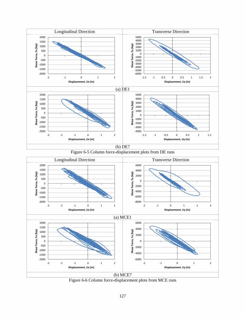
127
Longitudinal Direction Transverse Direction
(a) DE1
(b) DE7
Figure 6-5 Column force-displacement plots from DE runs
Longitudinal Direction Transverse Direction
(a) MCE1
(b) MCE7
Figure 6-6 Column force-displacement plots from MCE runs
-2000
-1500
-1000
-500
0
500
1000
1500
2000
-2 -1 0 1 2
Shea
r Fo
rce
, Fx
(kip
)
Displacement, Ux (in)
-6000-5000-4000-3000-2000-1000
010002000300040005000
-1.5 -1 -0.5 0 0.5 1 1.5 2
She
ar F
orc
e, F
y (k
ip)
Displacement, Uy (in)
-2000
-1500
-1000
-500
0
500
1000
1500
2000
-3 -2 -1 0 1 2
Shea
r Fo
rce
, Fx
(kip
)
Displacement, Ux (in)
-4000
-3000
-2000
-1000
0
1000
2000
3000
4000
5000
-1.5 -1 -0.5 0 0.5 1 1.5Sh
ear
Fo
rce
, Fy
(kip
)
Displacement, Uy (in)
-2000
-1500
-1000
-500
0
500
1000
1500
2000
-3 -2 -1 0 1 2
Shea
r Fo
rce
, Fx
(kip
)
Displacement, Ux (in)
-8000
-6000
-4000
-2000
0
2000
4000
6000
-2 -1 0 1 2 3
She
ar F
orc
e, F
y (k
ip)
Displacement, Uy (in)
-2000
-1500
-1000
-500
0
500
1000
1500
2000
-3 -2 -1 0 1 2
Shea
r Fo
rce
, Fx
(kip
)
Displacement, Ux (in)
-6000
-4000
-2000
0
2000
4000
6000
-2 -1 0 1 2
She
ar F
orc
e, F
y (k
ip)
Displacement, Uy (in)

128
(a) ductility ratios in the longitudinal direction
(b) ductility ratios in the transverse direction
Figure 6-7 Summary of column Displacement ductility
0.0
0.5
1.0
1.5
2.0
2.5
Dis
pla
cem
en
t D
uct
ility
Ground Motion
Ex. II-1b Column Displ. Ductility: Longitudinal Dir.
0.0
0.5
1.0
1.5
2.0
2.5
3.0
3.5
4.0
4.5
Dis
pla
cem
en
t D
uct
ility
Ground Motion
Ex. II-1b Column Displ Ductility: Transverse Dir.

129
Chapter 7 Bridge with Two-Column Piers Designed using Type 2
Strategy (Example II-2)
7.1 Bridge Description
The overall geometry of Ex. II-2 is described in Section 1.3.2. From the final design iteration, the
reinforced concrete (R/C) column diameter is 5 ft-6in. with 2.8% longitudinal steel ratio and 2.6%
transverse steel ratio. The rectangular pier cap is 6 ft-6in. wide and 5 ft-6 in. deep. The pier cap is 60 ft
long and the center-to-center distance between the columns is 40 ft. Figure 7-1 shows the elevation at
piers. The cross-frames are of X-type pattern with diagonal members made of L4x4x1/2 single angles
while the top and bottom chords are 2L2x2x1/4 double angles.
7.2 Computational Model
The computational model is shown in Figure 7-2. The equivalent concrete section properties of
superstructure are summarized in Table 7-1. Local axes of the superstructure are shown in Figure 7-1.
Deck cracking was accounted for in the calculation of these properties by using 50% of the gross concrete
modulus of elasticity (Ec).
For elastic analysis, only one of the diagonal members of the cross-frames is included in the model as
shown in Figure 7-2b. This is because the cross-frames are designed and detailed to yield and buckle
under the design earthquake. Under transverse loading, in each cross-frame panel, one diagonal is under
tension and the other is in compression. Consequently, the diagonal in compression would buckle and its
stiffness becomes essentially zero.
For nonlinear response history analysis, the cross-frames were modeled with multi-linear plastic link
elements with force-deformation relationship shown in Figure 1-5. The two cross-frame diagonal
members are modeled because buckling is accounted for in the definition of link force-deformation
relationship. Calculation of expected force and deformations are shown in Sections 7.5 and 7.6.
Table 7-1 Ex.II-1 superstructure section properties
Area, A (in2) 16,195
Moment of inertia about horizontal axis, I2 (in4) 10,316,084
Moment of inertia about vertical axis, I3 (in4) 8.22 x 10
8
Torsional constant, J (in4) 285,124

130
Figure 7-1 Elevation at pier of Ex. II-2
7.3 Analysis
7.3.1 Gravity Loads – DC and DW
The total DC load (i.e. total bridge dead load) is 3,933 kips and the total DW load is 844 kips. The
reactions at the base of each column due to these loads are 904 kips and 166 kips, respectively. These
loads were used to calculate the effective section properties of the columns, as illustrated in Section 7.3.2
Steps 1 and 2.
2
3

131
Figure 7-2 Analytical model of Ex. II-2
(a) 3D view of model
(b) Detail at piers
(c) Detail at abutments
Beam element located at
superstructure c.g.
Columns and pier cap = beam
element
Link element
to transfer
superstructure
vertical and
longitudinal
forces to
bearings
x
z
y
Rigid beam element
located at deck c.g.
Rigid links to connect rigid
beam element to top chord
Gap link element
Soil link element
Link element for
vertical support only
(i.e. free to translate
in any horizontal
direction)
Cross-frames = beam
elements in elastic analysis,
multi-linear plastic link
elements in nonlinear
analysis.

132
7.3.2 Earthquake Loads – EQ
Step 1: Calculate column axial loads due to
gravity loads, Pcol.
This will be used to determine the effective
moment of inertia, Ie, of columns.
( ) ( )
Step 2: Determine effective moment of inertia, Ie.
This is accomplished through section analysis of
the column. The required parameters are: column
diameter, longitudinal and transverse
reinforcements, axial load, and material properties
of concrete and steel reinforcement.
The calculated Ie is assigned to the beam elements
representing the column in the model.
The following are the column properties:
D = 5.5 ft
ρl = 2.8% (66 - #11)
ρs = 2.6% (#8 @ 2.0 in.)
f’c = 4 ksi
fy = 60 ksi
Pcol = 1,379 kips
From section analysis:
Ie/Ig = 0.57
Step 3: Estimate soil displacement, Δsoil, and
calculate the effective abutment stiffness, Ke.
The joint gap is included in the calculation of this
stiffness, as shown in the figure below.
Figure 7-3 Abutment force-displacement
The soil passive resistance, Pp, and initial soil
stiffness, Ki, are calculated based on the
recommended values in Caltrans SDC.
( ⁄ ) ( )
( ⁄ ) ( )
where Ae (ft2) is the effective backwall area, h (ft)
is the backwall height, and w is the backwall
Δsoil = 3.3 in.
( )( ⁄ )
( )( ⁄ )
Check Δsoil against Δgap + Δy to determine if the
soil is yielding.
Since this is smaller than Δsoil, the soil is yielding
and the effective stiffness is:

133
width.
Under EQ in longitudinal direction, only one
abutment is engaged in one direction. To account
for this in elastic analyses such as modal and
response spectrum analysis, half of Ke is applied to
both abutments.
This 1/2Ke is then distributed to the link elements
representing the soil. The gap link elements shown
in Figure 7-2c were assigned with high stiffness
with no opening during elastic analysis.
Since there are 12 soil springs at each abutment,
the effective stiffness assigned to each is:
( )
Step 4: Perform modal analysis and determine the
required number of modes needed for multimode
spectral analysis.
After the effective stiffnesses of the elements are
determined, modal analysis is performed to
determine the fundamental vibration periods and
the required number of modes needed in the
response spectrum analysis. The AASHTO
Specifications requires that the total number of
modes used should ensure participation of at least
90% of the total bridge mass.
Table 7-2 shows the result of modal analysis.
Although only the first 5 modes are shown in this
table, a total of 30 modes were used in the
response spectrum analysis with total mass
participation of 100% in both the longitudinal
and transverse directions.
The first mode with period of 0.64 sec is in-plane
deck rotation; the second with period of 0.61 sec
is the longitudinal translation mode; the third
with period of 0.57 sec is the vertical vibration
mode; and the fourth with period of 0.48 sec is
the longitudinal translation mode.
The vibration periods in this example are shorter
than those in Ex. II-1 because of larger columns.
Table 7-2 Modal periods and mass participation
Mode Period Mass Participation
No Sec x-dir y-dir
1 0.64 0.000 0.000
2 0.61 0.967 0.000
3 0.57 0.000 0.000
4 0.48 0.000 0.887
5 0.34 0.000 0.000
Step 5: Perform response spectrum analysis in the
longitudinal direction (EQx), determine Δsoil, and
check against the initial value in Step 3.
The design spectrum is applied in the longitudinal
direction. Multimode spectral analysis is used and
the modal responses are combined using the
Complete Quadratic Combination (CQC).
From response spectrum analysis, Δsoil = 3.26 in.
This is within 5% of the assumed displacement in
Step 3, thus no further iteration is needed.
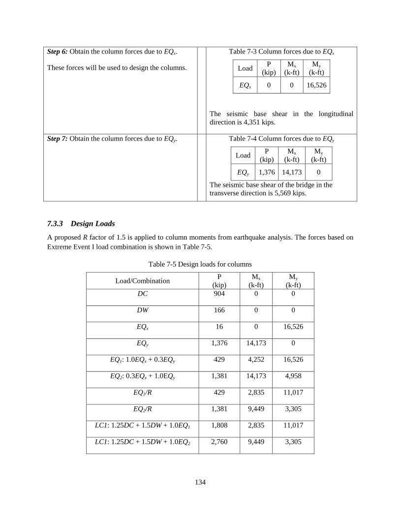
134
Step 6: Obtain the column forces due to EQx.
These forces will be used to design the columns.
Table 7-3 Column forces due to EQx
Load P
(kip)
Mx
(k-ft)
My
(k-ft)
EQx 0 0 16,526
The seismic base shear in the longitudinal
direction is 4,351 kips.
Step 7: Obtain the column forces due to EQy. Table 7-4 Column forces due to EQy
Load P
(kip)
Mx
(k-ft)
My
(k-ft)
EQy 1,376 14,173 0
The seismic base shear of the bridge in the
transverse direction is 5,569 kips.
7.3.3 Design Loads
A proposed R factor of 1.5 is applied to column moments from earthquake analysis. The forces based on
Extreme Event I load combination is shown in Table 7-5.
Table 7-5 Design loads for columns
Load/Combination P
(kip)
Mx
(k-ft)
My
(k-ft)
DC 904 0 0
DW 166 0 0
EQx 16 0 16,526
EQy 1,376 14,173 0
EQ1: 1.0EQx + 0.3EQy 429 4,252 16,526
EQ2: 0.3EQx + 1.0EQy 1,381 14,173 4,958
EQ1/R 429 2,835 11,017
EQ2/R 1,381 9,449 3,305
LC1: 1.25DC + 1.5DW + 1.0EQ1 1,808 2,835 11,017
LC1: 1.25DC + 1.5DW + 1.0EQ2 2,760 9,449 3,305

135
7.4 Design of Columns
Step 1: Determine the design axial load and
resultant moment from Section 7.3.3.
Table 7-6 Design axial load and resultant moment
Load
Combination
P
(kip)
Mres
(kip-ft)
LC1 1,808 11,376
LC2 2,760 10,010
Step 2: Develop the axial force-moment (P-M)
interaction curve and check if the design loads are
inside the P-M curve.
The AASHTO ϕ factors are used in the interaction
curve.
From the final iteration the column properties are:
D = 5.5 ft
ρl = 2.8% (61 - #11)
ρs = 2.6% (#8 @ 2.0 in.)
f’c = 4 ksi
fy = 60 ksi
The design loads are within the boundaries of P-
M interaction curve as shown below. Thus, the
selected column size and reinforcement are
adequate.
Step 3: Determine the plastic shear resistance, Fp,
of the piers in transverse direction
The plastic moment resistance, Mp, of column is a
function of its axial load. In multi-column pier,
due to frame action, there is variation in column
axial loads resulting in different plastic moment
capacities. Calculation of Fp is therefore an
iterative process. The calculation of Fp is outlined
in the procedure below.
0
2000
4000
6000
8000
10000
12000
0 2000 4000 6000 8000 10000 12000 14000
ϕP
n (
kip
s)
ϕMn (kip-ft)

136
Step 3.1: Start the calculation process by using the
column axial load, P, obtained from LC1.
Step 3.2: Based on this P, determine Mn from the
interaction curve.
Step 3.3: Determine Mp and Vp.
where the 1.3 factor is to account for column
overstrength.
where H is the column clear height. This equation
is based on double-curvature behavior. This
behavior is typically assumed for a multi-column
pier because the cap beam is much stiffer than the
columns.
Step 3.4: Calculate Fp and ΔP.
The following equations are based on the free-
body diagram for a two-column pier shown in
Figure 7-4.
Figure 7-4 Forces in a two-column pier
From Table 7-6, P = 1,808 kips.
Since this P was from response spectrum
analysis, both columns of the pier have the same
P.
By interpolating on the points of the interaction
curve, Mn = 12,751 kip-ft for P = 1,808 kips.
Mp = 1.3(12,751) = 16,576 kip-ft
Vp = 2(16,576)/20 = 1,658 kips
Fp
H
Vp1 Vp2Mp1 Mp1
ΔP ΔP

137
( ) ( )
where L is the distance between the two columns.
Step 3.5: Update the axial load in the columns.
Where P1 is the updated axial load in left column
and Pp is updated axial load in right column.
Step 3.6: Update the Mn, Mp, and Vp in the
columns.
The new plastic moments and shears are
determined using P1 and P2.
Step 3.7: Calculate the new Fp and ΔP and
compare against that in Step 3.4.
If Fp in this step is within 5% of that in Step 3.4,
further iteration is not necessary. Otherwise,
repeat Steps 3.4 to 3.7.
Step 3.8: Repeat Steps 3.1 to 3.7 using P from
LC2.
Fp = 1,658 + 1,658 = 3,316 kips
( ) ( )
P1 = 1,808 – 829 = 979 kips
P2 = 1,808 + 829 = 2,637 kips
For P1 = 979 kips
Mn1 = 12,366 kip-ft from interaction
curve
Mp1 = 1.3(12,366) = 16,076 kip-ft
Vp1 = 2(16,076)/20 = 1,608 kips
For P2 = 2,637 kips
Mn2 = 12,631 kip-ft from interaction
curve
Mp2 = 1.3(12,631) = 16,420 kip-ft
Vp2 = 2(17,268)/20 = 1,642 kips
Fp = 1,608 + 1,642 = 3,250 kips
( ) ( )
Since Fp and ΔP are within 5% of previous,
further iteration is not necessary.
The calculations were started using P = 2,760
kips from LC2 in Table 6-6. The results of the
last iteration are:
Mp1 = 16,567 kip-ft

138
Step 3.9: Determine the maximum Fp and the
maximum column plastic shear resistance.
This is the maximum of the results from Steps 3.7
and 3.8. The results will be used to design the
column transverse reinforcement and cross-
frames.
Vp1 = 1,657 kips
Mp2 = 15,876 kip-ft
Vp2 = 1,588 kips
Fp = 3,245 kips
From the results of Steps 3.7 and 3.8:
Vp = 1,657 kips (maximum Vp per column)
Fp = 3,250 kips (maximum Fp for the pier)
Step 4: Determine the column shear resistance
and compare against the plastic shear resistance.
The shear resistance can be calculated using the
Simplified Procedure described in AASHTO
Specifications Art. 5.8.3.4.1. For simplicity and to
be conservative, the contribution of concrete to
the shear resistance is not included in the
calculations.
where:
Ash = area of one leg of transverse reinforcement;
fy is the yield stress of transverse reinforcement; s
is the spacing of transverse reinforcement; D is
the diameter of column; Dr is the diameter of the
circle passing through the centers of longitudinal
reinforcement.
The transverse reinforcement is #8 rebar spaced
at 2.0 in. on center. The longitudinal
reinforcement is #11 rebar. The concrete cover is
2.0 in.
( )
( )
( )( )
( )
The maximum Vp = 1,657 kips per column.
The demand-resistance ratio is:

139
Step 5: Check the transverse reinforcement.
The volumetric ratio of transverse reinforcement
shall satisfy (AASHTO Specifications Art.
5.10.11.4.1d):
The spacing of transverse reinforcement shall
satisfy (AASHTO Specifications Art.
5.10.11.4.1e):
{
ρs = 2.6% (#8 @ 2.0 in.)
fy = 60 ksi
f’c = 4 ksi
(
)
{

140
7.5 Design of Ductile Cross-Frames
In the proposed Type 2 seismic design, the cross-frames are designed such that their resistance is less than
the column nominal shear resistance in the transverse direction so the inelasticity will be limited to the
cross-frames in that direction.
Step 1: Determine cross-frame force based on
nominal shear resistance of the pier.
The cross-frame shear force is equal to nominal
shear resistance of pier in the transverse direction.
where Fp is the pier plastic shear resistance.
The corresponding cross-frame diagonal member
axial force with R factor applied is:
where N is the number of panels, θ is the angle of
the diagonal from the horizontal, and R is the
cross-frame modification factor and is equal to
4.0. In this equation, only one diagonal is assumed
resisting the shear force. This is because, in a
panel, one diagonal is in tension and the other one
is in compression. The compression diagonal is
expected to buckle in which case its post-buckling
resistance is considerably smaller, thus the
resistance is largely due to the yield resistance of
the diagonal in tension.
Fp = 3,250 kips
N = 5
θ = 22o
( )
Step 2: Determine the cross-frame force from
response spectrum analysis in the transverse
direction.
Step 3: The design cross-frame force is the
smaller of PXF1 or PXF2.
PXF = 135 kips
Step 4: Determine cross-frame size.
The required area is:
A36 single angle
Fy = 36 ksi

141
where Fy is the nominal yield stress of the cross-
frame. The nominal value is used since PXF was
calculated from nominal shear force.
Note that the size of the cross-frame may be
governed by the compactness and slenderness
requirements shown in Step 5.
Use L4x4x1/2
Ag = 3.75 in2
rz = 0.776 in
I = 5.52 in4
x = 1.18 in. distance from connected leg of angle
to its c.g.
L = 142.62 in
Step 5: Check the compactness and slenderness
ratios.
The diagonal members of ductile cross-frames
shall satisfy (proposed AASHTO Specifications
Art. 6.16.4.5.2a):
√
The slenderness ratio shall satisfy (proposed
AASHTO Specifications Art. 6.16.4.5.2b):
√
where K is 0.85, l is taken as one-half of the
length of the diagonal member due to biased
buckling, r is the radius of gyration normal to the
plane of buckling and is equal to rz for single
angle members.
√
( )
√
Step 6: Calculate the expected yield resistance.
where Fye is the expected yield stress and is equal
to RyFy. For A36 steel sections, Ry = 1.5.
Fye = 1.5(36) = 54 ksi
( )( )
Step 7: Calculate the expected compressive
resistance.
The compressive resistance is calculated

142
according to AASHTO Specifications Art. 6.9.2.1,
6.9.4.1.1, and 6.9.4.1.2
(
)
o If Pe/Po > 0.44
[ ( ⁄ )]
o If Pe/Po < 0.44
( )
( ) ( )
( )
[ ( )]( )
Step 8: Calculate the maximum expected lateral
resistance of the cross-frames and compare against
the pier nominal shear resistance.
The maximum lateral resistance is the maximum
of:
( )
where Pt = 1.2Pye is the tensile resistance of the
diagonal member. The 1.5 factor is to account for
the upper bound of tensile resistance. The 0.3Pnc is
the post-buckling resistance of the diagonal
member. Vlat1 typically governs particularly with
relatively slender diagonal members. Vlat2 may
govern in cases when the diagonal members are
short and stocky.
The cross-frame maximum lateral resistance is
compared against the pier nominal shear
resistance to ensure elastic columns.
( )
[ ( )]
[ ( )]
Therefore, Vlat = 1,301 kips
Step 9: Determine the superstructure drift and
check against limit.
After the cross-frame designed, the superstructure
drift is determined. The superstructure lateral
displacement is calculated using the equation:
( )
( )

143
where, PEQY is the force in the cross-frame
diagonal member determined from response
spectrum analysis in the transverse direction and
Ae is the effective area calculated using Eqn.
(1-12).
The superstructure lateral drift should not exceed
4% (proposed AASHTO Specification Art.
6.16.4.5.1).
( )
( )
7.6 Cross-Frame Properties for Nonlinear Analysis
The expected force and displacement resistance of the cross-frames are calculated for use in the design
evaluation.
Step 1: Calculate the expected tensile yield
displacement.
The expected yield resistance is calculated in
Section 7.5 Step 6.
The effective axial stiffness is:
where E is the modulus of elasticity of steel which
is 29,000 ksi, Ae is the effective area calculated
using Eqn. (1-12), and L is the total length of the
diagonal member.
The expected yield displacement is then calculated
as:
L4x4x1/2
Pye = 202.5 kips
Ag = 3.75 in2
I = 5.52 in4
x = 1.18 in. distance from connected leg of angle
to its c.g.
( )
( )
( )
Step 2: Calculate the expected compressive
displacement.
The expected compressive resistance is calculated
in Section 7.5 Step 7.
Pnc = 125.10 kips

144
The corresponding displacement is:
7.7 Design Summary
The total weight of Ex. II-2 is 4,340 kips. From modal and response spectrum analyses, the periods,
forces, and displacements are:
Parameter Longitudinal Direction Transverse Direction
Fundamental period, T (sec) 0.61 0.48
Base shear, Vb (kip) 4,351 5,569
Column displacement demand, Δcol (in) 2.2 1.0
Column shear demand, Vcol (kip) 660 1,387
Pier base shear demand, Fb (kip) 1,320 2,774
Deck displacement demand, Δdeck (in) 3.35 2.25
The column properties are:
Diameter, D 5.5 ft
Longitudinal reinforcement 61 - #11 (ρl = 2.8%)
Transverse reinforcement #8 @ 2 in. (ρs = 2.6%)
Effective moment of inertia, Ie 0.57Ig
Column plastic shear resistance, Vp 1,657 kips
Pier plastic shear resistance, Fp 3,250 kips
The cross-frame diagonal member section properties are:
Section L4x4x1/2 (A36)
Area, Ag 3.75 in2
Slenderness ratio, KL/r 78.11
Width-thickness ratio, b/t 8.0
Expected tensile yield resistance, Pye 202.5 kips
Expected compressive resistance, Pnc 125.10 kips
Lateral resistance of cross-frames, Vlat 1,301 kips

145
7.8 Nonlinear Evaluation
Example II-2 was analyzed using the ground motions described in Section 1.8.1. The ground motions
were scaled to represent the Design (DE) and MCE Earthquake levels. There were seven DE runs and
seven MCE runs for a total of fourteen runs. Because of this, only the column force-displacement plots
from DE1, DE7, MCE1 and MCE7 are shown in Figure 7-5 and Figure 7-6 to represent the results.
However, the column ductility ratios for all runs are shown in Figure 7-7.
The yield displacements were calculated according to Section 1.8.2. Since the expected material
properties were used in the nonlinear analyses, the yield displacements were also calculated using these
properties. The yield displacements are 1.47 in. and 0.66 in. in the longitudinal and transverse directions,
respectively.
In the longitudinal direction, the average ductility ratios were 1.6 from DE runs and 1.9 from MCE runs.
In the transverse direction, the respective ductility ratios were 1.3 and 1.4. The longitudinal ductility
ratios are comparable to those from Ex. II-1b while the transverse ductility ratios are about half. The
yielding cross-frames limited the seismic forces transmitted to the column in the transverse direction
resulting in lower ductility ratios. The columns were elastic even at MCE.
Figure 7-8 and Figure 7-9 shows the superstructure force-displacement in the transverse direction under
DE1, DE7, MCE1, and MCE7. As shown, there was significant yielding in the support cross-frames. It
can be observed that the transverse shear force in the superstructure is about the same as the column
transverse base shear, with the superstructure shear force slightly less.
The average of total bearing forces in the transverse direction was 1,543 kips under DE and 1,554 kips
under MCE. This is larger than the cross-frame lateral resistance shown in Section 7.7 because the cross-
frames did not yield and buckle and at the same time which, in turn, is due to flexibility of the pier cap.
Note that the tensile and post-buckling resistances of the cross-frame were used in the calculation of
lateral resistance. The average column base shear forces in the transverse directions were 1,920 kips
under DE and 2,065 kips under MCE. These are below the pier plastic resistance of 3,250 kips shown in
Section 7.7. For this bridge, the inertia force in the pier cap is about 20% of the base shear.
The average lateral displacement of the superstructure under DE was 2.02 in. (3.7% drift). This is larger
than the displacement calculated from the cross-frame design shown in Section 7.5 Step 9 (the
displacement is 1.56 in. and the drift is 2.9%). This difference is attributed to the larger contribution of the
higher modes to the superstructure transverse response. Figure 1-8 shows that the selected ground
motions have higher spectral accelerations at short periods.

146
Longitudinal Direction Transverse Direction
(a) DE1
(b) DE7
Figure 7-5 Column force-displacement plots from DE runs
Longitudinal Direction Transverse Direction
(a) MCE1
(b) MCE7
Figure 7-6 Column force-displacement plots from MCE runs
-1500
-1000
-500
0
500
1000
1500
-3 -2 -1 0 1 2
Shea
r Fo
rce
, Fx
(kip
)
Displacement, Ux (in)
-2000
-1500
-1000
-500
0
500
1000
1500
2000
2500
-1 -0.5 0 0.5 1
She
ar F
orc
e, F
y (k
ip)
Displacement, Uy (in)
-1500
-1000
-500
0
500
1000
1500
-3 -2 -1 0 1 2 3
Shea
r Fo
rce
, Fx
(kip
)
Displacement, Ux (in)
-2000
-1500
-1000
-500
0
500
1000
1500
2000
-1 -0.5 0 0.5 1Sh
ear
Fo
rce
, Fy
(kip
)
Displacement, Uy (in)
-1500
-1000
-500
0
500
1000
1500
-3 -2 -1 0 1 2 3
Shea
r Fo
rce
, Fx
(kip
)
Displacement, Ux (in)
-2000
-1500
-1000
-500
0
500
1000
1500
2000
2500
-1 -0.5 0 0.5 1
She
ar F
orc
e, F
y (k
ip)
Displacement, Uy (in)
-1500
-1000
-500
0
500
1000
1500
-4 -3 -2 -1 0 1 2 3
Shea
r Fo
rce
, Fx
(kip
)
Displacement, Ux (in)
-2000
-1500
-1000
-500
0
500
1000
1500
2000
2500
-1 -0.5 0 0.5 1
She
ar F
orc
e, F
y (k
ip)
Displacement, Uy (in)

147
(a) ductility ratios in the longitudinal direction
(b) ductility ratios in the transverse direction
Figure 7-7 Summary of column Displacement ductility
0.0
0.5
1.0
1.5
2.0
2.5D
isp
lace
me
nt
Du
ctili
ty
Ground Motion
Ex. II-2 Column Displ. Ductility: Longitudinal Dir.
0.0
0.2
0.4
0.6
0.8
1.0
1.2
1.4
1.6
1.8
Dis
pla
cem
en
t D
uct
ility
Ground Motion
Ex. II-2 Column Displ Ductility: Transverse Dir.

148
(a) DE1 (b) DE7
Figure 7-8 Superstructure force-displacement in the transverse direction from DE runs
(a) MCE1 (b) MCE7
Figure 7-9 Superstructure force-displacement in the transverse direction from MCE runs
-2000
-1500
-1000
-500
0
500
1000
1500
2000
-2 -1 0 1 2 3 4
Tota
l Brg
Sh
ear
Forc
e, F
y (k
ip)
Girder Displacement (in)
-2000
-1500
-1000
-500
0
500
1000
1500
-2.5 -2 -1.5 -1 -0.5 0 0.5
Tota
l Brg
Sh
ear
Forc
e, F
y (k
ip)
Girder Displacement (in)
-2000
-1500
-1000
-500
0
500
1000
1500
2000
-4 -2 0 2 4
Tota
l Brg
Sh
ear
Forc
e, F
y (k
ip)
Girder Displacement (in)
-2000
-1500
-1000
-500
0
500
1000
1500
2000
-3 -2 -1 0 1 2 3
Tota
l Brg
Sh
ear
Forc
e, F
y (k
ip)
Girder Displacement (in)

149
Chapter 8 Bridge with Wall Piers Design using Type 1 Strategy
(Example III-1)
8.1 Bridge Description
The overall geometry of Ex. III-1 is described in Section 1.3.3. From the final design iteration, the
reinforced concrete (R/C) wall pier is 40 ft wide and 4 ft thick. The vertical and horizontal steel
reinforcement ratios are both 0.69% (#9 spaced at 6 in.). Figure 8-1 shows the elevation at piers. The
cross-frames are of X-type pattern with diagonal members made of L8x8x1 single angles while the top
and bottom chords are 2L4x4x1/2 double angles.
8.2 Computational Model
The extruded view of the computational model is shown in Figure 8-2 and details of the model are shown
in Figure 8-3. The equivalent concrete section properties of superstructure are summarized in Table 8-1.
Local axes of the superstructure are shown in Figure 8-1. Deck cracking was accounted for in the
calculation of these properties by using 50% of the gross concrete modulus of elasticity (Ec).
The wall pier was modeled as a vertical beam element as shown in Figure 8-3a. The top of wall is then
connected to a horizontal rigid beam element where the link elements representing the bearings are
connected as shown in Figure 8-3b. To ensure correct modeling of the boundary condition at the top of
the wall, the nodes of the horizontal beam element are assigned with rigid constraint such that there is no
relative deformation and rotation between them.
For nonlinear response history analysis, the cross-frames were modeled with multi-linear plastic link
element with force-deformation relationship shown in Figure 1-5 to account for inelasticity in case it
occurred. Calculation of expected force and deformations are shown in Section 8.6.
Table 8-1 Ex.II-1 superstructure section properties
Area, A (in2) 16,195
Moment of inertia about horizontal axis, I2 (in4) 10,316,084
Moment of inertia about vertical axis, I3 (in4) 8.22 x 10
8
Torsional constant, J (in4) 285,124

150
Figure 8-1 Elevation at pier of Ex. III-1
Figure 8-2 Extruded view of analytical model of Ex. III-1
2
3

151
Figure 8-3 Analytical model of Ex. III-1
(a) 3D view of model
(b) Detail at piers
(c) Detail at abutments
Beam element located at
superstructure c.g.
Walls and pier cap = beam
element
Link element to
transfer
superstructure
vertical and
longitudinal
forces to bearings
x
z y
Rigid beam element
located at deck c.g.
Rigid links to connect rigid
beam element to top chord
Gap link element
Soil link element
Link element for
vertical support only
(i.e. free to translate
in any horizontal
direction)
Cross-frames =
beam elements in
elastic analysis,
multi-linear plastic
link elements in
nonlinear analysis.
Rigid beam element
located at on top
ofwall Nodes along the top of wall are
assigned with rigid constraints

152
8.3 Analysis
8.3.1 Gravity Loads – DC and DW
The total DC load (i.e. total bridge dead load) is 4,704 kips and the total DW load is 844 kips. The
reactions at the base of wall due to these loads are 1,991 kips and 332 kips, respectively. These loads were
used to calculate the effective section properties, as illustrated in Section 8.3.2 Steps 1 and 2.
8.3.2 Earthquake Loads – EQ
Step 1: Calculate wall axial loads due to gravity
loads, Pcol.
This will be used to determine the effective
moment of inertia, Ie, of columns.
( ) ( )
Step 2: Determine effective moment of inertia, Ie.
This is accomplished through section analysis of
the wall. The required parameters are: wall
dimensions, longitudinal and transverse
reinforcements, axial load, and material properties
of concrete and steel reinforcement.
The calculated Ie is assigned to the beam elements
representing the wall pier in the model.
The following are the column properties:
w = 40 ft
t = 4 ft
ρv = 0.69% (#9 at 6 in. both face for a total of 158
- #9)
ρh = 0.69% (#9 @ 6 in.)
f’c = 4 ksi
fy = 60 ksi
Pcol = 2,787 kips
From section analysis:
Ie/Ig = 0.24
Step 3: Estimate soil displacement, Δsoil, and
calculate the effective abutment stiffness, Ke.
The joint gap is included in the calculation of this
stiffness, as shown in the figure below.
Δsoil = 3.75 in.
( )( ⁄ )
( )( ⁄ )
Check Δsoil against Δgap + Δy to determine if the
soil is yielding.

153
Figure 8-4 Abutment force-displacement
The soil passive resistance, Pp, and initial soil
stiffness, Ki, are calculated based on the
recommended values in Caltrans SDC.
( ⁄ ) ( )
( ⁄ ) ( )
where Ae (ft2) is the effective backwall area, h (ft)
is the backwall height, and w is the backwall
width.
Under EQ in longitudinal direction, only one
abutment is engaged in one direction. To account
for this in elastic analyses such as modal and
response spectrum analysis, half of Ke is applied to
both abutments.
This 1/2Ke is then distributed to the link elements
representing the soil. The gap link elements shown
in Figure 8-3c were assigned with high stiffness
with no opening during elastic analysis.
Since this is smaller than Δsoil, the soil is yielding
and the effective stiffness is:
Since there are 12 soil springs at each abutment,
the effective stiffness assigned to each is:
( )
Step 4: Perform modal analysis and determine the
required number of modes needed for multimode
spectral analysis.
After the effective stiffnesses of the elements are
determined, modal analysis is performed to
determine the fundamental vibration periods and
the required number of modes needed in the
response spectrum analysis. The AASHTO
Specifications requires that the total number of
modes used should ensure participation of at least
90% of the total bridge mass.
Table 8-2 shows the result of modal analysis.
Although only the first 7 modes are shown in this
table, a total of 30 modes were used in the
response spectrum analysis with total mass
participation of 100% in both the longitudinal
and transverse directions.
The first mode with period of 0.67 sec is
longitudinal translation mode; the second with
period of 0.57 sec is the vertical vibration mode;
the transverse translation modes are the fifth and
seventh modes with periods of 0.30 sec and 0.17
sec, respectively.
Table 8-2 Modal periods and mass participation
Mode Period Mass Participation
No Sec x-dir y-dir
1 0.67 0.900 0.000
2 0.57 0.000 0.000
3 0.35 0.000 0.000
4 0.34 0.000 0.000
5 0.30 0.000 0.420
6 0.29 0.000 0.000
7 0.17 0.000 0.390

154
Step 5: Perform response spectrum analysis in the
longitudinal direction (EQx), determine Δsoil, and
check against the initial value in Step 3.
The design spectrum is applied in the longitudinal
direction. Multimode spectral analysis is used and
the modal responses are combined using the
Complete Quadratic Combination (CQC).
From response spectrum analysis, Δsoil = 3.72 in.
This is within less than 5% of the assumed value,
thus, no further iteration is needed.
Step 6: Obtain the column forces due to EQx.
These forces will be combined with the forces due
to EQy to determine the design forces.
Table 8-3 Column forces due to EQx
Load P
(kip)
Mx
(k-ft)
My
(k-ft)
EQx 37 0 27,326
The seismic base shear of the bridge in the
longitudinal direction is 4,014 kips.
Step 7: Perform response spectrum analysis in the
transverse direction (EQy) and determine the
column forces.
Table 8-4 Column forces due to EQy
Load P
(kip)
Mx
(k-ft)
My
(k-ft)
EQy 0 75,952 0
The seismic base shear of the bridge in the
transverse direction is 5,095 kips.

155
8.3.3 Design Loads
The 100%-30% combination was used to combine the EQx and EQy forces. The results are shown in
Table 8-5.
Table 8-5 Combination of forces due to EQx and EQy
Load/Combination P
(kip)
Mx
(k-ft)
My
(k-ft)
EQx 37 0 27,326
EQy 0 75,952 0
EQ1: 1.0EQx + 0.3EQy 37 22,786 27,326
EQ2: 0.3EQx + 1.0EQy 11 75,952 8,198
The response modification factor, R, is then applied to EQ1 and EQ2 moments. The piers are designed as
wall in both directions thus R is equal to 2.0. The resulting forces are then combined with DC and DW
forces to determine the design forces. The load factors are based on Extreme Event I load combination
and the result is shown in Table 8-6.
Table 8-6 Design loads
Load/Combination P
(kip)
Fx
(kip)
Fy
(kip)
Mx
(k-ft)
My
(k-ft)
DC 1,991 0 0 0 0
DW 332 0 0 0 0
EQ1/R 37 568 382 11,393 13,663
EQ2/R 11 171 1,274 37,976 4,099
LC1: 1.25DC + 1.5DW + 1.0EQ1 3,024 568 382 11,393 13,663
LC2: 1.25DC + 1.5DW + 1.0EQ2 2,998 171 1,274 37,976 4,099
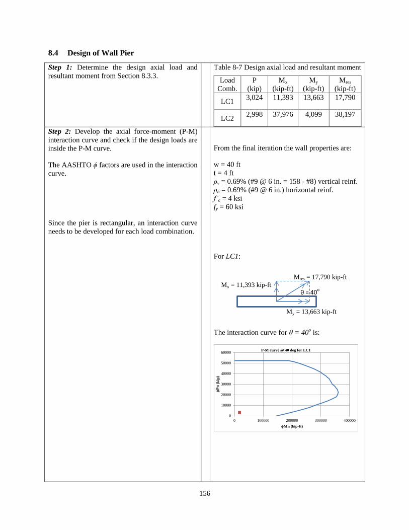
156
8.4 Design of Wall Pier
Step 1: Determine the design axial load and
resultant moment from Section 8.3.3.
Table 8-7 Design axial load and resultant moment
Load
Comb.
P
(kip)
Mx
(kip-ft)
My
(kip-ft)
Mres
(kip-ft)
LC1 3,024 11,393 13,663 17,790
LC2 2,998 37,976 4,099 38,197
Step 2: Develop the axial force-moment (P-M)
interaction curve and check if the design loads are
inside the P-M curve.
The AASHTO ϕ factors are used in the interaction
curve.
Since the pier is rectangular, an interaction curve
needs to be developed for each load combination.
From the final iteration the wall properties are:
w = 40 ft
t = 4 ft
ρv = 0.69% (#9 @ 6 in. = 158 - #8) vertical reinf.
ρh = 0.69% (#9 @ 6 in.) horizontal reinf.
f’c = 4 ksi
fy = 60 ksi
For LC1:
The interaction curve for θ = 40o is:
0
10000
20000
30000
40000
50000
60000
0 100000 200000 300000 400000
ϕP
n (
kip
)
ϕMn (kip-ft)
P-M curve @ 40 deg for LC1
Mx = 11,393 kip-ft
My = 13,663 kip-ft
θ = 40o
Mres = 17,790 kip-ft

157
Since the design of the wall section is governed
by the forces in the weak axis direction, the
capacity in this direction is also checked against
the forces due to earthquake in longitudinal
direction EQx.
For LC2:
The interaction curve for θ = 84o is:
For EQx:
P = 3,024
My = 13,663 kip-ft (R = 2)
The interaction curve for θ = 0o is:
Therefore, selected section and its reinforcement
are adequate.
Step 3: Determine shear resistance in the
transverse direction.
Transverse direction is the strong direction of the
wall.
ρh = 0.0069
b = 48 in.
d = 472 in.
0
10000
20000
30000
40000
50000
60000
0 50000 100000 150000 200000 250000 300000 350000ϕ
Pn
(k
ip)
ϕMn (kip-ft)
P-M curve @ 84 deg for LC2
0
10000
20000
30000
40000
50000
60000
0 10000 20000 30000 40000 50000
ϕP
n (
kip
)
ϕMn (kip-ft)
P-M curve @ 0 deg for EQx
Mx = 37,976 kip-ft
My = 4,099 kip-ft
θ = 84o
Mres = 38,197 kip-ft

158
The factored shear resistance, Vr, of the wall pier
is taken as the lesser of (AASHTO Specifications
Art. 5.10.11.4.2):
√ and
[ √ ]
where ρh is the horizontal steel reinforcement
ratio.
√ ( )( )
[ √ ( )]( )( )
Therefore, Vr = 11,011 kips
The maximum shear demand is 1,274 kips from
Table 8-6.
Step 5: Check the vertical and horizontal
reinforcements.
The minimum vertical and horizontal
reinforcement ratio shall satisfy (AASHTO
Specifications Art. 5.10.11.4.2):
The spacing of vertical and horizontal
reinforcement shall satisfy (AASHTO
Specifications Art. 5.10.11.4.2):

159
8.5 Seismic Design of Cross-Frames
Step 1: Determine the design cross-frame force.
Designing the cross-frames based on shear
resistance of wall pier may result in large
uneconomical section due to large shear resistance
of wall piers. Therefore, in this case, the diagonal
member design force is taken as the lesser of:
( )
and
where N is the number of cross-frame panels, θ is
the angle of the diagonal member measured from
the horizontal, and PEQY is the force in the
diagonal member from response spectrum analysis
in the transverse direction.
Vr = 11,011 kips
N = 5 panels
θ = 22 degrees
( )( )
From response spectrum analysis in the
transverse direction:
Therefore, the design axial load in the diagonal
member is:
Step 2: Cross-frame member section properties.
Note that the size of the cross-frames may be
governed by slenderness requirements.
Section: L8x8x1
Fy = 36 ksi
Ag = 15.0 in2
rx = ry = 2.43 in.
rz = 1.56 in.
L = 142.62 in.
Step 3: Calculate the tensile resistance
( )( )
Step 4: Calculate the compressive resistance
Under seismic loading, the cross-frames are
primary members in the transverse direction as
they transmit the deck seismic forces to the
bearings. The limiting slenderness ratio for
primary members is 120 (AASHTO Specifications
Art. 6.9.3).
Equal-leg single angle sections will be used as
diagonal members. The slenderness ratio is
calculated according to AASHTO Specifications
l/rx = 142.62/2.43 = 58.69 < 80
(
)
( )

160
Art. 6.9.4.4.
o If l/rx < 80
(
)
o If l/rx > 80
(
)
The compressive resistance is calculated
according to AASHTO Specifications Art. 6.9.2.1,
6.9.4.1.1, and 6.9.4.1.2
(
)
The slender element reduction factor, Q, is equal
to 1.0 when:
√
o If Pe/Po > 0.44
[ ( ⁄ )]
o If Pe/Po < 0.44
( )
Note that although the calculations shown here is
for single angle sections, double angles may be
also used as diagonal members of cross-frames
under Type 1 design strategy.
( )
( )
√
( )( )
[ ]( )
Step 5: Calculate the minimum nominal shear
resistance of the cross-frames
( )
In this equation, only the compression resistance,
Pn, is used to determine the minimum nominal
shear resistance. Note that Pn is smaller than the
(
)
This is less than the nominal shear resistance of
the wall pier:

161
tensile resistance, Pr, which means buckling
would occur first in any of the diagonal members
before yielding is reached. Thus, VXF is the
minimum shear force before inelasticity starts to
occur in the cross-frames.
Although this is Type 1 design strategy, VXF may
be less than shear resistance of the wall pier. As
noted in Step 1, in cases where the pier shear
resistance is very large, the cross-frames are
designed based on the response spectrum analysis.
This means that cross-frames may become
inelastic before shear resistance of pier is reached.
8.6 Cross-Frame Properties for Nonlinear Analysis
The expected force and displacement resistance of the cross-frames are calculated for use in the design
evaluation.
Step 1: Calculate the expected tensile yield and
displacement resistance.
The expected yield resistance is:
where Fye is the expected yield stress and is equal
to RyFy. For A36 steel sections, Ry = 1.5.
The effective axial stiffness is:
where E is the modulus of elasticity of steel which
is 29,000 ksi, Ae is the effective area calculated
using Eqn. (1-12), and L is the total length of the
diagonal member.
The expected yield displacement is then calculated
as:
L8x8x1
Fye = 1.5(36) = 54 ksi
Ag = 15.0 in2
I = 89.1 in4
x = 2.40 in. distance from connected leg of angle
to its c.g.
( )
( )
( )
( )

162
Step 2: Calculate the expected compressive
resistance and associated displacement.
The (Kl/r)eff and Pe is the same as that calculated
in Section 8.5 Step 4. The expected yield strength
is used to calculate Po.
The expected compressive resistance is then
calculated as:
o If Pe/Po > 0.44
[ ( ⁄ )]
o If Pe/Po < 0.44
The corresponding displacement is:
( )( )
( )
8.7 Design Summary
The total weight of Ex. III-1 is 4,383 kips. From modal and response spectrum analyses, the periods,
forces, and displacements are:
Parameter Longitudinal Direction Transverse Direction
Fundamental period, T (sec) 0.67 0.31
Base shear, Vb (kip) 4,014 5,151
Pier displacement, Δpier (in) 4.76 0.21
Pier Base Shear, Fb (kip) 1,136 2,576
Deck displacement, Δdeck (in) 3.74 0.61
The wall pier properties are:
Width, w 40 ft
Thickness, t 4 ft
Vertical reinforcement #9 @ 6 in. (total 158 - #8) (ρv = 0.69%)
Horizontal reinforcement #9 @ 6 in. (ρh = 0.69%)
Factored shear resistance, Vr 11,011 kips

163
The cross-frame diagonal member section properties are:
Section L8x8x1 (A36)
Area, A 15.0 in2
Slenderness ratio, KL/r 116.02
Width-thickness ratio, b/t 8.0
Tensile resistance, ϕPr 513 kips
Compressive resistance, ϕPn 239 kips
Min. nominal shear resistance, VXF_min 2,466 kips
Expected tensile yield resistance, Pye 810 kips
Expected compressive resistance, Pnc 280 kips

164
8.8 Nonlinear Evaluation
Example III-1 was analyzed using the ground motions described in Section 1.8.1. The ground motions
were scaled to represent the Design (DE) and MCE Earthquake levels. There were seven DE runs and
seven MCE runs for a total of fourteen runs. Because of this, only the column force-displacement plots
from DE1, DE7, MCE1 and MCE7 are shown in Figure 8-5 and Figure 8-6 to represent the results.
However, the column ductility ratios in the longitudinal direction for all runs are shown in Figure 8-7.
Only the results in longitudinal direction are shown here because the transverse displacements were small
and piers were elastic. The cross-frames remained elastic in all runs.
The yield displacements were calculated according to Section 1.8.2. Since the expected material
properties were used in the nonlinear analyses, the yield displacements were also calculated using these
properties. The yield displacement in the longitudinal direction is 2.07 in. The average ductility ratios
were 1.8 from DE runs and 2.5 from MCE runs.
The negative stiffness observed in the hysteresis plots was not due to instability in the structure or
computational error in the analysis. Rather, it is attributed to the coupled biaxial response of the column.
This phenomenon was observed when the response is elastic and depends on the frequency content of the
input motion and period of the structure (Monzon et al. 2013b).
Figure 8-8 shows the transverse base shear forces in the wall piers. The average base shear at DE runs
was 3,500 kips and at MCE it was 4,800 kips which were below the transverse shear resistance of the wall
pier shown in Section 8.7. The average of total bearing shear forces in the transverse direction were 3,207
kips under DE and 4,393 kips under MCE. These are below the expected lateral resistance of the cross-
frames which is equal to 4,896 kips, thus the cross-frame were elastic.

165
Longitudinal Direction Transverse Direction
(a) DE1
(b) DE7
Figure 8-5 Column force-displacement plots from DE runs
Longitudinal Direction Transverse Direction
(a) MCE1
(b) MCE7
Figure 8-6 Column force-displacement plots from MCE runs
-1500
-1000
-500
0
500
1000
1500
-4 -2 0 2 4 6
Shea
r Fo
rce
(ki
p)
Displacement (in)
-5000
-4000
-3000
-2000
-1000
0
1000
2000
3000
-0.2 -0.1 0 0.1 0.2 0.3
Shea
r Fo
rce
(ki
p)
Displacement (in)
-1000
-500
0
500
1000
1500
-4 -2 0 2 4
Shea
r Fo
rce
(ki
p)
Displacement (in)
-5000
-4000
-3000
-2000
-1000
0
1000
2000
3000
4000
5000
-0.3 -0.2 -0.1 0 0.1 0.2 0.3
Shea
r Fo
rce
(ki
p)
Displacement (in)
-1500
-1000
-500
0
500
1000
1500
-6 -4 -2 0 2 4 6
Shea
r Fo
rce
(ki
p)
Displacement (in)
-6000
-5000
-4000
-3000
-2000
-1000
0
1000
2000
3000
4000
5000
-0.3 -0.2 -0.1 0 0.1 0.2 0.3 0.4
Shea
r Fo
rce
(ki
p)
Displacement (in)
-1500
-1000
-500
0
500
1000
1500
-6 -4 -2 0 2 4 6
Shea
r Fo
rce
(ki
p)
Displacement (in)
-6000
-4000
-2000
0
2000
4000
6000
-0.4 -0.2 0 0.2 0.4
Shea
r Fo
rce
(ki
p)
Displacement (in)

166
Figure 8-7 Summary of column displacement ductility in the longitudinal direction
Figure 8-8 Summary of wall base shear in the transverse direction
0.0
0.5
1.0
1.5
2.0
2.5
3.0
3.5
4.0
Dis
pla
cem
en
t D
uct
ility
Ground Motion
Ex. III-1 Wall Displ. Ductility: Longitudinal Dir.
0
1000
2000
3000
4000
5000
6000
She
ar F
orc
e, F
y (k
ip)
Ground Motion
Wall Base Shear: Transverse Direction

167
Chapter 9 Bridge with Wall Piers Designed using Type 2 Strategy
(Example III-2)
9.1 Bridge Description
The overall geometry of Ex. III-2 is described in Section 1.3.3. From the final design iteration, the
reinforced concrete (R/C) wall pier is 40 ft wide and 4 ft thick. The vertical and horizontal steel
reinforcement ratios are both 0.69% (#9 spaced at 6 in.). Figure 9-1 shows the elevation at piers. The
cross-frames are of X-type pattern with diagonal members made of L4x4x3/4 single angles while the top
and bottom chords are 2L2x2x3/8 double angles
9.2 Computational Model
The extruded view of the computational model is shown in Figure 9-2 and details of the model are shown
in Figure 9-3. The equivalent concrete section properties of superstructure are summarized in Table 9-1.
Local axes of the superstructure are shown in Figure 9-1. Deck cracking was accounted for in the
calculation of these properties by using 50% of the gross concrete modulus of elasticity (Ec).
For elastic analysis, only one of the diagonal members of the cross-frames is included in the model as
shown in Figure 9-3b. This is because the cross-frames are designed and detailed to yield and buckle
under the design earthquake. Under transverse loading, in each cross-frame panel, one diagonal is under
tension and the other is in compression. Consequently, the diagonal in compression would buckle and its
stiffness becomes essentially close to zero.
For nonlinear response history analysis, the cross-frames were modeled with multi-linear plastic link
elements with force-deformation relationship shown in Figure 1-5. The two cross-frame diagonal
members are modeled because buckling is accounted for in the definition of link force-deformation
relationship. Calculation of expected force and deformations are shown in Sections 9.5 and 9.6.
Table 9-1 Ex.II-1 superstructure section properties
Area, A (in2) 16,195
Moment of inertia about horizontal axis, I2 (in4) 10,316,084
Moment of inertia about vertical axis, I3 (in4) 8.22 x 10
8
Torsional constant, J (in4) 285,124

168
Figure 9-1 Elevation at piers of Ex. III-2
Figure 9-2 Extruded view of analytical model of Ex. III-2
2
3

169
Figure 9-3 Analytical model of Ex. III-2
(a) 3D view of model
(b) Detail at piers
(c) Detail at abutments
Beam element located at
superstructure c.g.
Walls and pier cap = beam
element
Link element
to transfer
superstructure
vertical and
longitudinal
forces to
bearings
x
z y
Rigid beam element
located at deck c.g.
Rigid links to connect rigid
beam element to top chord
Gap link element
Soil link element
Link element for
vertical support only
(i.e. free to translate
in any horizontal
direction)
Cross-frames =
beam elements in
elastic analysis,
multi-linear plastic
link elements in
nonlinear analysis.
Rigid beam element
located at on top
ofwall Nodes along the top of wall are
assigned with rigid constraints
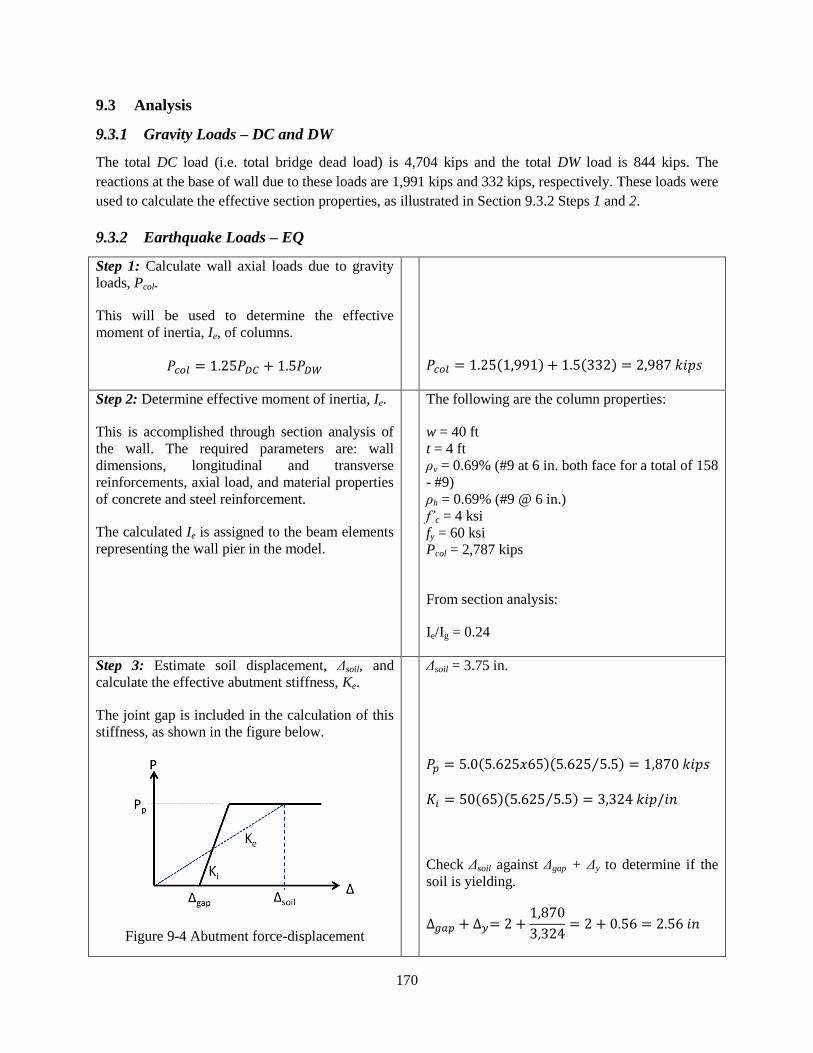
170
9.3 Analysis
9.3.1 Gravity Loads – DC and DW
The total DC load (i.e. total bridge dead load) is 4,704 kips and the total DW load is 844 kips. The
reactions at the base of wall due to these loads are 1,991 kips and 332 kips, respectively. These loads were
used to calculate the effective section properties, as illustrated in Section 9.3.2 Steps 1 and 2.
9.3.2 Earthquake Loads – EQ
Step 1: Calculate wall axial loads due to gravity
loads, Pcol.
This will be used to determine the effective
moment of inertia, Ie, of columns.
( ) ( )
Step 2: Determine effective moment of inertia, Ie.
This is accomplished through section analysis of
the wall. The required parameters are: wall
dimensions, longitudinal and transverse
reinforcements, axial load, and material properties
of concrete and steel reinforcement.
The calculated Ie is assigned to the beam elements
representing the wall pier in the model.
The following are the column properties:
w = 40 ft
t = 4 ft
ρv = 0.69% (#9 at 6 in. both face for a total of 158
- #9)
ρh = 0.69% (#9 @ 6 in.)
f’c = 4 ksi
fy = 60 ksi
Pcol = 2,787 kips
From section analysis:
Ie/Ig = 0.24
Step 3: Estimate soil displacement, Δsoil, and
calculate the effective abutment stiffness, Ke.
The joint gap is included in the calculation of this
stiffness, as shown in the figure below.
Figure 9-4 Abutment force-displacement
Δsoil = 3.75 in.
( )( ⁄ )
( )( ⁄ )
Check Δsoil against Δgap + Δy to determine if the
soil is yielding.

171
The soil passive resistance, Pp, and initial soil
stiffness, Ki, are calculated based on the
recommended values in Caltrans SDC.
( ⁄ ) ( )
( ⁄ ) ( )
where Ae (ft2) is the effective backwall area, h (ft)
is the backwall height, and w is the backwall
width.
Under EQ in longitudinal direction, only one
abutment is engaged in one direction. To account
for this in elastic analyses such as modal and
response spectrum analysis, half of Ke is applied to
both abutments.
This 1/2Ke is then distributed to the link elements
representing the soil. The gap link elements shown
in Figure 8-3c were assigned with high stiffness
with no opening during elastic analysis.
Since this is smaller than Δsoil, the soil is yielding
and the effective stiffness is:
Since there are 12 soil springs at each abutment,
the effective stiffness assigned to each is:
( )
Step 4: Perform modal analysis and determine the
required number of modes needed for multimode
spectral analysis.
After the effective stiffnesses of the elements are
determined, modal analysis is performed to
determine the fundamental vibration periods and
the required number of modes needed in the
response spectrum analysis. The AASHTO
Specifications requires that the total number of
modes used should ensure participation of at least
90% of the total bridge mass.
Table 9-2 shows the result of modal analysis.
Although only the first 5 modes are shown in this
table, a total of 30 modes were used in the
response spectrum analysis with total mass
participation of 100% in both the longitudinal
and transverse directions.
The first mode with period of 0.67 sec is
longitudinal translation mode; the second with
period of 0.57 sec is the vertical vibration mode;
the transverse translation mode is the fourth
mode with period of 0.39 sec. This transverse
mode is mainly due to deformation in the support
cross-frames. The third mode with a period of
0.52 sec is in-plane torsional mode.
Table 9-2 Modal periods and mass participation
Mode Period Mass Participation
No Sec x-dir y-dir
1 0.67 0.904 0.000
2 0.57 0.000 0.000
3 0.52 0.000 0.000
4 0.39 0.000 0.722
5 0.34 0.000 0.000

172
Step 5: Perform response spectrum analysis in the
longitudinal direction (EQx), determine Δsoil, and
check against the initial value in Step 3.
The design spectrum is applied in the longitudinal
direction. Multimode spectral analysis is used and
the modal responses are combined using the
Complete Quadratic Combination (CQC).
From response spectrum analysis, Δsoil = 3.72 in.
This is within less than 5% of the assumed value,
thus, no further iteration is needed.
Step 6: Obtain the column forces due to EQx.
These forces will be combined with the forces due
to EQy to determine the design forces.
Table 9-3 Column forces due to EQx
Load P
(kip)
Mx
(k-ft)
My
(k-ft)
EQx 37 0 27,326
The seismic base shear of the bridge in the
longitudinal direction is 4,014 kips.
Step 6: Obtain the column forces due to EQy.
Table 9-4 Column forces due to EQy
Load P
(kip)
Mx
(k-ft)
My
(k-ft)
EQy 0 86,468 0
The seismic base shear of the bridge in the
longitudinal direction is 5,771 kips.

173
9.3.3 Design Loads
A proposed R factor of 1.5 is applied to the moments from earthquake analysis. The forces based on
Extreme Event I load combination is shown in Table 9-5.
Table 9-5 Design loads for wall pier
Load/Combination P
(kip)
Mx
(k-ft)
My
(k-ft)
DC 1,991 0 0
DW 332 0 0
EQx 37 0 27,326
EQy 0 86,468 0
EQ1: 1.0EQx + 0.3EQy 37 25,940 27,326
EQ2: 0.3EQx + 1.0EQy 11 86,468 8,198
EQ1/R 37 17,293 18,217
EQ2/R 11 57,645 5,465
LC1: 1.25DC + 1.5DW + 1.0EQ1 3,024 17,293 18,217
LC1: 1.25DC + 1.5DW + 1.0EQ2 2,998 57,645 5,465
9.4 Design of Wall Pier
Step 1: Determine the design axial load and
resultant moment from Section 9.3.3.
Table 9-6 Design axial load and resultant moment
Load
Comb.
P
(kip)
Mx
(kip-ft)
My
(kip-ft)
LC1 3,024 17,293 18,217
LC2 2,998 57,645 5,465
Step 2: Develop the axial force-moment (P-M)
interaction curve and check if the design loads are
inside the P-M curve.
The AASHTO ϕ factors are used in the interaction
curve.
From the final iteration the wall properties are:
w = 40 ft
t = 4 ft
ρv = 0.69% (#9 @ 6 in. = 158 - #8) vertical reinf.
ρh = 0.69% (#9 @ 6 in.) horizontal reinf.
f’c = 4 ksi

174
Since the pier is rectangular, an interaction curve
needs to be developed for each load combination.
fy = 60 ksi
For LC1:
Note: the x- and y-axes are based on global axes.
The interaction curve for θ = 46o is:
For LC2:
The interaction curve for θ = 85o is:
0
10000
20000
30000
40000
50000
60000
0 50000 100000 150000 200000 250000 300000 350000
ϕP
n (
kip
)
ϕMn (kip-ft)
P-M curve @ 44 deg for LC1
0
10000
20000
30000
40000
50000
60000
0 50000 100000 150000 200000 250000 300000 350000
ϕP
n (
kip
)
ϕMn (kip-ft)
P-M curve @ 85 deg for LC1
Mx = 57,645 kip-ft
My = 5,465 kip-ft
θ = 85o
Mres = 57,903 kip-ft
Mx = 17,293 kip-ft
My = 18,217 kip-ft
θ = 44o
Mres = 25,118 kip-ft

175
Since the design of the wall section is governed
by the forces in the weak axis direction, the
capacity in this direction is also checked against
the forces due to earthquake in longitudinal
direction EQx.
For EQx:
P = 3,024
My = 18,217 kip-ft (R = 1.5)
The interaction curve for θ = 0o is:
Therefore, selected section and its reinforcement
are adequate.
Step 3: Determine shear resistance in the
transverse direction.
Transverse direction is the strong direction of the
wall.
The factored shear resistance, Vr, of the wall pier
is taken as the lesser of (AASHTO Specifications
Art. 5.10.11.4.2):
√ and
[ √ ]
where ρh is the horizontal steel reinforcement
ratio.
ρh = 0.0069
b = 48 in.
d = 472 in.
√ ( )( )
[ √ ( )]( )( )
Therefore, Vr = 11,011 kips
Step 5: Check the vertical and horizontal
reinforcements.
The minimum vertical and horizontal
reinforcement ratio shall satisfy (AASHTO
Specifications Art. 5.10.11.4.2):
The spacing of vertical and horizontal
0
10000
20000
30000
40000
50000
60000
0 10000 20000 30000 40000 50000
ϕP
n (
kip
)
ϕMn (kip-ft)
P-M curve @ 0 deg for EQx

176
reinforcement shall satisfy (AASHTO
Specifications Art. 5.10.11.4.2):

177
9.5 Design of Ductile Cross-Frames
Step 1: Determine cross-frame force based on
nominal shear resistance of the pier.
The cross-frame shear force is equal to nominal
shear resistance of pier in the transverse direction.
where Vr is the factored shear resistance of wall
pier.
The corresponding cross-frame diagonal member
axial force with R factor applied is:
where N is the number of panels, θ is the angle of
the diagonal from the horizontal, and R is the
cross-frame modification factor and is equal to
4.0. In this equation, only one diagonal is assumed
resisting the shear force. This is because, in a
panel, one diagonal is in tension and the other one
is in compression. The compression diagonal is
expected to buckle in which case its post-buckling
resistance is considerably smaller, thus the
resistance is largely due to the yield resistance of
the diagonal in tension.
Vr = 11,011 kips
N = 5
θ = 22o
( )
Step 2: Determine the cross-frame force from
response spectrum analysis in the transverse
direction.
Step 3: The design cross-frame force is the
smaller of PXF1 or PXF2.
In bridges with wall piers, it is expected that PXF2
would govern due to large shear resistance of
wall.
PXF = 152.43 kips
Step 4: Determine cross-frame size.
The required area is:
A36 single angle
Fy = 36 ksi

178
where Fy is the nominal yield stress of the cross-
frame. The nominal value is used since PXF was
calculated from nominal shear force.
Note that the size of the cross-frame may be
governed by the compactness and slenderness
requirements shown in Step 5.
Use L4x4x3/4
Ag = 5.44 in2
rz = 0.774 in
I = 7.62 in4
x = 1.27 in. distance from connected leg of angle
to its c.g.
L = 142.62 in
Step 5: Check the compactness and slenderness
ratios.
The diagonal members of ductile cross-frames
shall satisfy (proposed AASHTO Specifications
Art. 6.16.4.5.2a):
√
The slenderness ratio shall satisfy (proposed
AASHTO Specifications Art. 6.16.4.5.2b):
√
where K is 0.85, l is taken as one-half of the
length of the diagonal member due to biased
buckling, r is the radius of gyration normal to the
plane of buckling and is equal to rz for single
angle members.
√
( )
√
Step 6: Calculate the expected yield resistance.
where Fye is the expected yield stress and is equal
to RyFy. For A36 steel sections, Ry = 1.5.
Fye = 1.5(36) = 54 ksi
( )
Step 7: Calculate the expected compressive
resistance.
The compressive resistance is calculated

179
according to AASHTO Specifications Art. 6.9.2.1,
6.9.4.1.1, and 6.9.4.1.2
(
)
The slender element reduction factor, Q, is equal
to 1.0 when:
√
o If Pe/Po > 0.44
[ ( ⁄ )]
o If Pe/Po < 0.44
( )
( ) ( )
√
( )( )
[ ( )]( )
Step 8: Calculate the maximum expected lateral
resistance of the cross-frames and compare against
the pier nominal shear resistance.
The maximum lateral resistance is the maximum
of:
( )
where Pt = 1.2Pye is the tensile resistance of the
diagonal member. The 1.5 factor is to account for
the upper bound of tensile resistance. The 0.3Pnc is
the post-buckling resistance of the diagonal
member. Vlat1 typically governs particularly with
relatively slender diagonal members. Vlat2 may
govern in cases when the diagonal members are
short and stocky.
The cross-frame maximum lateral resistance is
compared against the pier nominal shear
resistance to ensure elastic response.
( )
[ ( )]( )
[ ( )]( )
Therefore, Vlat = 2,295 kips
Step 9: Determine the superstructure drift and
check against limit.

180
After the cross-frame designed, the superstructure
drift is determined. The superstructure lateral
displacement is calculated using the equation:
where, PEQY is the force in the cross-frame
diagonal member determined from response
spectrum analysis in the transverse direction and
Ae is the effective area calculated using Eqn.
(1-12).
The superstructure lateral drift should not exceed
4% (proposed AASHTO Specification Art.
6.16.4.5.1).
( )
( )
( )
( )
9.6 Cross-Frame Properties for Nonlinear Analysis
The expected force and displacement resistance of the cross-frames are calculated for use in the design
evaluation.
Step 1: Calculate the expected tensile yield
displacement.
The expected yield resistance is calculated in
Section 9.5 Step 6.
The effective axial stiffness is:
where E is the modulus of elasticity of steel which
is 29,000 ksi, Ae is the effective area calculated
using Eqn. (1-12), and L is the total length of the
diagonal member.
The expected yield displacement is then calculated
as:
L4x4x3/4
Pye = 293.76 kips
Ag = 5.44 in2
I = 7.62 in4
x = 1.27 in. distance from connected leg of angle
to its c.g.
( )
( )
( )
Step 2: Calculate the expected compressive
displacement.

181
The expected compressive resistance is calculated
in Section 9.5 Step 7.
The corresponding displacement is:
Pnc = 181.00 kips
9.7 Design Summary
The total weight of Ex. III-2 is 4,374 kips. From modal and response spectrum analyses, the periods,
forces, and displacements are:
Parameter Longitudinal Direction Transverse Direction
Fundamental period, T (sec) 0.67 0.39
Base shear, Vb (kip) 4,014 5,771
Pier displacement, Δpier (in) 3.57 0.15
Pier Base Shear, Fb (kip) 1,136 2,885
Deck displacement, Δdeck (in) 3.74 1.39
The wall pier properties are:
Width, w 40 ft
Thickness, t 4 ft
Vertical reinforcement #9 @ 6 in. (total 158 - #9) (ρv = 0.69%)
Horizontal reinforcement #9 @ 6 in. (ρh = 0.69%)
Factored shear resistance, Vr 11,011 kips
The cross-frame diagonal member section properties are:
Section L4x4x3/4 (A36)
Area, A 5.44 in2
Expected tensile yield resistance, Pye 294 kips
Expected compressive resistance, Pnc 181 kips
Maximum lateral resistance, Vlat 2,295 kips
182
9.8 Nonlinear Evaluation
Example III-2 was analyzed using the ground motions described in Section 1.8.1. The ground motions
were scaled to represent the Design (DE) and MCE Earthquake levels. There were seven DE runs and
seven MCE runs for a total of fourteen runs. Because of this, only the column force-displacement plots
from DE1, DE7, MCE1 and MCE7 are shown in Figure 9-5 and Figure 9-6 to represent the results.
However, the column ductility ratios in the longitudinal direction for all runs are shown in Figure 9-7.
Only the results in longitudinal direction are shown here because the transverse displacements were small
and piers were elastic.
The yield displacements were calculated according to Section 1.8.2. Since the expected material
properties were used in the nonlinear analyses, the yield displacements were also calculated using these
properties. The yield displacement in the longitudinal direction is 2.07 in. The average ductility ratios
were 1.8 from DE runs and 2.5 from MCE runs which are the same as those from Example III-1.
The negative stiffness observed in the hysteresis plots was not due to instability in the structure or
computational error in the analysis. Rather, it is attributed to the coupled biaxial response of the column.
This phenomenon was observed when the response is elastic and depends on the frequency content of the
input motion and period of the structure (Monzon et al. 2013b).
Figure 9-8 shows the transverse base shear forces in the wall piers. Both DE and MCE runs have an
average base shear of 2,700 kips. They were the same because the yielding cross-frames limited the
seismic force in the transverse direction. At DE, this base shear is 75% of the base shear from Example
III-1. At MCE, it is 57% of the base shear from Example III-1. The average of total bearing forces under
DE and MCE is both 2,224 kips which is about the same as the expected lateral resistance of the cross-
frames shown in Section 9.7.
Figure 9-9 and Figure 9-10 shows the superstructure force-displacement in the transverse direction under
DE1, DE7, MCE1, and MCE7. As shown, there was significant yielding in the support cross-frames. It
can be observed that the transverse shear force in the superstructure is about the same as the column
transverse base shear, with the superstructure shear force slightly less. The difference is attributed to the
inertia force in the wall pier.
The average lateral displacement of the superstructure under DE was 1.61 in. (3% drift). This is larger
than the displacement calculated from the cross-frame design shown in Section 9.5 Step 9 (the
displacement is 1.28 in. and the drift is 2.4%). This difference is attributed to the larger contribution of the
higher modes to the superstructure transverse response. Figure 1-8 shows that the selected ground
motions have higher spectral accelerations at short periods.

183
Longitudinal Direction Transverse Direction
(a) DE1
(b) DE7
Figure 9-5 Column force-displacement plots from DE runs
Longitudinal Direction Transverse Direction
(a) MCE1
(b) MCE7
Figure 9-6 Column force-displacement plots from MCE runs
-1500
-1000
-500
0
500
1000
1500
-4 -2 0 2 4 6
Shea
r Fo
rce
(ki
p)
Displacement (in)
-4000
-3000
-2000
-1000
0
1000
2000
3000
-0.2 -0.1 0 0.1 0.2
Shea
r Fo
rce
(ki
p)
Displacement (in)
-1000
-500
0
500
1000
1500
-4 -2 0 2 4
Shea
r Fo
rce
(ki
p)
Displacement (in)
-3000
-2000
-1000
0
1000
2000
3000
-0.2 -0.1 0 0.1 0.2
Shea
r Fo
rce
(ki
p)
Displacement (in)
-1500
-1000
-500
0
500
1000
1500
-6 -4 -2 0 2 4 6
Shea
r Fo
rce
(ki
p)
Displacement (in)
-4000
-3000
-2000
-1000
0
1000
2000
3000
-0.2 -0.1 0 0.1 0.2
Shea
r Fo
rce
(ki
p)
Displacement (in)
-1500
-1000
-500
0
500
1000
1500
-6 -4 -2 0 2 4 6
Shea
r Fo
rce
(ki
p)
Displacement (in)
-3000
-2000
-1000
0
1000
2000
3000
-0.2 -0.1 0 0.1 0.2
Shea
r Fo
rce
(ki
p)
Displacement (in)

184
Figure 9-7 Summary of column displacement ductility in the longitudinal direction
Figure 9-8 Summary of wall base shear in the transverse direction
0.0
0.5
1.0
1.5
2.0
2.5
3.0
3.5D
isp
lace
me
nt
Du
ctili
ty
Ground Motion
Ex. III-2 Wall Displ. Ductility: Longitudinal Dir.
0
500
1000
1500
2000
2500
3000
3500
She
ar F
orc
e, F
y (k
ip)
Ground Motion
Wall Base Shear: Transverse Direction

185
(a) DE1 (b) DE7
Figure 9-9 Superstructure force-displacement in the transverse direction from DE runs
(a) MCE1 (b) MCE7
Figure 9-10 Superstructure force-displacement in the transverse direction from MCE runs
-2500
-2000
-1500
-1000
-500
0
500
1000
1500
2000
2500
-1 0 1 2 3 4
Shea
r Fo
rce
(ki
p)
Displacement (in)
-2500
-2000
-1500
-1000
-500
0
500
1000
1500
2000
2500
-1.5 -1 -0.5 0 0.5 1 1.5
Shea
r Fo
rce
(ki
p)
Displacement (in)
-2500
-2000
-1500
-1000
-500
0
500
1000
1500
2000
2500
-2 -1 0 1 2 3 4
Shea
r Fo
rce
(ki
p)
Displacement (in)
-2500
-2000
-1500
-1000
-500
0
500
1000
1500
2000
2500
-3 -2 -1 0 1 2
Shea
r Fo
rce
(ki
p)
Displacement (in)

186
Chapter 10 Summary of Design and Nonlinear Evaluation
10.1 Overview
The DECF system is one of the several techniques that can be used to reduce ductility in the columns and
may be used to protect the columns from damage during an earthquake. One advantage of this system
over other forms of seismic protection is the smaller superstructure and substructure displacements.
However, the beneficial effect of DECF is diminished when: (a) the pier is designed flexible and (b) when
the pier has large ductility demand (i.e. large R factor) in the longitudinal direction. The DECF system
works effectively when it is more flexible than the pier below it. If the pier is more flexible, then it will
yield before the cross-frames undergo inelasticity. The benefit of the DECF is also diminished when the
piers are designed to have large ductility demand in the longitudinal direction. In such case, the bridge
response would be dominated by the longitudinal response and the columns would yield even though the
DECF system limits the transverse seismic forces transferred to the columns.
Experimental and analytical investigations showed that DECF reduces the force and displacement
demand in the transverse direction of the substructure. However, the DECF is ineffective in the
longitudinal direction for a straight bridge due to its location and orientation. The nonlinear analysis of
bridges designed using Type 2 strategy showed that the bridge response in one direction affects the total
response. For example, the reduction of force in the column in the transverse direction reduces the overall
(resultant) force in the column. This overall response is important particularly when minimal damage or
bridge serviceability is required after an earthquake.
The nonlinear analysis of the design examples showed that the bridge responded as intended indicating
the adequacy of the proposed design procedure for Type 2 strategy. There was minimal yielding in the
columns such that they are considered essentially elastic even under the MCE-level earthquakes.
10.2 Design Examples Summary
The design using Types 1 and 2 strategies are summarized in Table 10-1 and the bridge response from
elastic multimodal spectral analysis is summarized Table 10-2. For bridges with single and two-column
piers, two bridges were designed using the Type 1 strategy – a bridge under operational category of
‘Other’ and a bridge under ‘Critical’ category. The bridges in the former were designed based on R-factor
of 3.0 (for single-column pier) and 5.0 (for two-column pier) while in the latter the R-factors were both
1.5. The two categories were used to show which bridge category the DECF is more effective. A more
direct comparison between the responses of ‘Critical’ bridge with Type 1 strategy and bridge with Type 2
strategy can be made because the R-factor used in both is 1.5. For the bridge with wall piers, since the R-
factors are about the same – 2.0 for ‘Other’ category and 1.5 for ‘Critical’ – only one example was
designed with Type 1 strategy. The design using either category would result in the same design.

187
As shown in Table 10-1, Ex. I-1a and II-1a resulted in smaller column because of larger R-factor.
However, bridges with Type 2 strategy (Ex. I-2 and II-2) has smaller column than the ‘Critical’ bridges
with Type 1 strategy (Ex. I-1b and II-1b) even though both use the same R-factor of 1.5. The flexibility
provided by DECF to the superstructure in the transverse direction reduced the overall demand in the
column. On the other hand, the larger cross-frame size needed in Type 1 strategy increases the transverse
bridge stiffness which further increases the seismic force that resulted in larger column.
Table 10-1 Summary of design
Pier
Type
Example
No.
Oper.
Category
Design
Strategy Pier Size
Reinforcement Support Cross-
Frames Long. Trans.
Single-
column
I-1a Other Type 1 4 ft diameter 1% 1% L8x8x5/8
I-1b Critical Type 1 6.5 ft diameter 2.4% 1.1% WT7x34
I-2 --- Type 2 5.5 ft diameter 2.5% 1% L3x3x3/8
Two-
column
II-1a Other Type 1 4 ft diameter 1% 1.4% L8x8x5/8
II-1b Critical Type 1 6.5 ft diameter 2.4% 2.5% WT9x65
II-2 --- Type 2 5.5 ft diameter 2.8% 2.6% L4x4x1/2
Wall III-1 Other Type 1 40 ft wide, 4 ft thick 0.69% 0.69% L8x8x1
III-2 --- Type 2 40 ft wide, 4 ft thick 0.69% 0.69% L4x4x3/4
Table 10-2 Summary of elastic seismic analysis
Example
No.
Fundamental Period
(sec)
Bridge Base Shear
(kip)
Bridge Deck Displacement
(in)
Longitudinal Transverse Longitudinal Transverse Longitudinal Transverse
I-1a 0.92 2.23 1,285 524 4.92 11.58
I-1b 0.49 0.58 2,780 1,354 2.8 3.2
I-2 0.58 1.22 2,150 973 3.18 5.78
II-1a 0.94 0.68 2,676 3,731 5.06 3.37
II-1b 0.51 0.35 5,722 6,681 2.97 0.97
II-2 0.61 0.48 4,351 5,569 3.35 2.25
III-1 0.67 0.31 4,014 5,151 3.74 0.61
III-2 0.67 0.39 4,014 5,771 3.74 1.39

188
10.3 Summary of Nonlinear Evaluations
The displacement ductility ratios are primarily used to compare the seismic response of the design
examples. Even though they the pier have the same number of columns, each example is essentially a
different bridge thus it is not fair to directly compare response parameters such as column displacements.
The bearing forces are used to show the benefit of allowing the cross-frames to go nonlinear. But the
comparison can only be made between ‘Critical’ bridge with Type 1 strategy and bridge with Type 2
strategy because both use the same R-factor and the columns remained essentially elastic in most cases.
For the two examples with wall piers, the bearing forces are the only parameter used to compare the
response because both have the same wall size and the wall remained elastic. The superstructure response
is summarized using the maximum drift ratios.
10.3.1 Bridge with Single-Column Piers
It is shown in Table 10-3 that the column displacement ductility ratios in the longitudinal direction are
about the same. Even though the columns are of different sizes, the ductility demand in this direction is
limited by the soil response at the abutments.
In the transverse direction, Ex. I-1a has the largest ductility demand because of smaller column. Only the
column resist the seismic forces in this direction thus the response is dependent on the column flexibility
only. The ductility demand in Ex. I-1b is considerably low such that the column can be considered as
essentially elastic, but this is expected since the R-factor used in the design is equal to 1.50. However, the
ductility demand in Ex. I-2 is smaller compared to Ex. I-1b and is even about half at MCE. The DECF in
Ex. I-2 limited the transverse forces transferred to the column resulting in less ductility demand even
though its column is more flexible than Ex. I-1b. This is evident in Table 10-4 where it shown that the
total bearing force in Ex. I-2 is about half of that in Ex. I-1b. For Ex. I-1a the bearing forces at DE and
MCE are about the same because of column yielding. In this example, it was the column plastic shear
force that limited the bearing forces.
The superstructure transverse displacements and corresponding drift ratios for Ex. I-2 are shown in Figure
10-1. The average drifts were 3.6 % under DE and 6.4% under MCE. The corresponding ductility
demands in the cross-frames were 3.9 and 6.9.
Table 10-3 Average column displacement ductility in bridges with single-column piers
Example
Average Column Displacement Ductility
Design EQ MCE
Longitudinal Transverse Longitudinal Transverse
I-1a 1.5 2.4 1.9 3.1
I-1b 1.5 1.6 1.8 2.1
I-2 1.5 1.0 1.9 1.2

189
Table 10-4 Average of total bearing force in the transverse direction
Example Average ∑Vbrg_trans (kips)
Design EQ MCE
I-1a 126 128
I-1b 575 641
I-2 257 274
Figure 10-1 Summary of superstructure transverse displacement and drift ratios
10.3.2 Bridge with Two-Column Piers
The observations made in bridges with single-column pier are also true for bridges with two-column
piers. The longitudinal ductility demands are about the same for all bridges. The transverse ductility
demands in the column of bridge designed based on Type 2 strategy are about half of those in ‘Critical’
bridge designed based on Type 1 strategy. The total transverse bearing forces in Ex. II-2 are less than half
of those in Ex. II-1b.
The superstructure transverse displacements and corresponding drift ratios for Ex. I-2 are shown in Figure
10-2. The average drifts were 3.7 % under DE and 5.3% under MCE. The corresponding ductility
demands in the cross-frames were 3.6 and 5.1.
0.0
0.8
1.5
2.3
3.1
3.8
4.6
5.4
6.2
0
0.5
1
1.5
2
2.5
3
3.5
4
4.5
DE1 DE2 DE3 DE4 DE5 DE6 DE7
Dri
ft (
%)
Sup
ers
tru
ctu
re T
ran
s. D
isp
l. (
in)

190
Table 10-5 Average column displacement ductility in bridges with two-column piers
Example
Average Column Displacement Ductility
Design EQ MCE
Longitudinal Transverse Longitudinal Transverse
II-1a 1.7 3.8 2.3 5.2
II-1b 1.6 2.0 1.9 2.9
II-2 1.6 1.3 1.9 1.4
Table 10-6 Average of total bearing force in the transverse direction
Example Average ∑Vbrg_trans (kips)
Design EQ MCE
II-1a 902 1010
II-1b 3,372 4,018
II-2 1,534 1,554
Figure 10-2 Summary of superstructure transverse displacement and drift ratios
10.3.3 Bridge with Wall Piers
In the longitudinal direction, the pier ductility demands in Ex. III-1 and III-2 are the same because both
have the same pier size. In the transverse direction, the pier is stiff and has large shear capacity thus it
remained elastic. The only difference between the two examples is the magnitude of transverse bearing
0.0
0.9
1.9
2.8
3.7
4.6
5.6
0
0.5
1
1.5
2
2.5
3
3.5
DE1 DE2 DE3 DE4 DE5 DE6 DE7
Dri
ft (
%)
Sup
ers
tru
ctu
re T
ran
s. D
isp
l. (
in)

191
forces as shown in Table 10-7. In Ex. III-2, the bearing force was limited by the DECF and it was the
same for both DE and MCE.
The superstructure transverse displacements and corresponding drift ratios for Ex. I-2 are shown in Figure
10-3. The average drifts were 3.0 % under DE and 4.8% under MCE. The corresponding ductility
demands in the cross-frames were 2.6 and 4.2.
Table 10-7 Average of total bearing force in the transverse direction
Example Average ∑Vbrg_trans (kips)
Design EQ MCE
III-1 3,206 4,393
II-2 2,224 2,224
Figure 10-3 Summary of superstructure transverse displacement and drift ratios
10.4 Concluding Remarks
This report presents a proposed ‘force-based’ design procedure that will achieve an essentially elastic
substructure and ductile superstructure. The reinforced concrete (R/C) substructure flexural resistance is
designed for the combined effect of seismic forces similar to conventional seismic design with a force
reduction factor equal to 1.5. Meanwhile, the shear resistance and the confinement requirements of the
substructure are determined in a way similar to the seismic design of conventional bridges. To achieve a
ductile superstructure, the horizontal resistance of the support cross frames is based on the lesser of the
pier nominal shear resistance and the elastic seismic cross forces obtained from the response spectrum
analysis, divided by a proposed response modification factor for ductile cross frames equal to 4. This will
ensure that support cross frames will act as a ‘fuse’ and will not subject the substructure to forces that
0.0
0.9
1.9
2.8
3.7
4.6
5.6
0
0.5
1
1.5
2
2.5
3
3.5
DE1 DE2 DE3 DE4 DE5 DE6 DE7
Dri
ft (
%)
Sup
ers
tru
ctu
re T
ran
s. D
isp
l. (
in)

192
may cause nonlinear response in that direction. To achieve a ductile response of support cross frames, the
diagonal members, which are expected to undergo inelastic response, are detailed to have limits on width-
to-thickness and slenderness ratios. The other cross frame components and the shear resistance of the
substructure are then checked for a fully yielded and strain hardened support cross frame.
The nonlinear seismic evaluation of the design examples verified the seismic performance of bridge
design according to the proposed Type 2 bridges. The inelasticity was concentrated at the support cross
frames while the substructure remained elastic. Furthermore, this evaluation showed the substructure also
remained essentially elastic even for ground motions at the MCE level. The main advantages of utilizing
Type 2 design strategy can be realized in post-earthquake repair since the substructure will remain elastic
while only the nonlinear elements that need to be replaced is the end cross frames. This performance may
be also achieved by using Type 1 performance criteria with critical bridges, however, the size of the cross
frames that is required for this design will be substantially larger than the one obtained using type 2. This
will require larger cross frames, bearings, and foundation.
The nonlinear seismic analysis also showed that stiff substructure i.e. pier walls shows great advantages
of using this strategy. The ductile end cross frames provide a “fuse” for the seismic forces and thus limits
the force transfer to the pier wall and to its foundation. Furthermore, the seismic analysis of conventional
design of example III-1 showed that the superstructure experienced nonlinear activity and subjected to the
bearing to forces that are not designed for. The failure of these bearing may cause unseating of the
superstructure if adequate support length was not provided on the top of the pier wall.

193
References
AASHTO. 2012. AASHTO LRFD Bridge Design Specifications, American Association of State Highway
and Transportation Officials, Washington, D.C.
AASHTO. 2012. AASHTO Guide Specifications for LRFD Bridge Seismic Design, American Association
of State Highway and Transportation Officials, Washington, D.C.
ASCE. 2010. Minimum Design Loads for Buildings and Other Structures, American Society of Civil
Engineers, Reston, VA.
AISC. 2010a. Specifications for Structural Steel Buildings, American Institute of Steel Construction,
Chicago, IL.
AISC. 2010b. Seismic Provisions for Structural Steel Buildings, American Institute of Steel Construction,
Chicago, IL.
Alfawakhiri, F. and Bruneau, M. 2001. “Local versus Global Ductility Demands in Simple Bridges,”
Journal of Structural Engineering, 127(5), 554-560.
Astaneh-Asl, A., Goel, S.C. and Hanson, R.D., 1985, Cyclic Out-of-Plane Buckling of Double Angle
Bracing. Report UCB/CE-STEEL-94/01. Department of Civil Engineering, University of California at
Berkeley, Berkeley, CA.
Bahrami, H., Itani, A.M., and Buckle, I.G. 2010. Guidelines for the Seismic Design of Ductile End Cross-
Frames in Steel Girder Bridge Superstructures, CCEER Report No. 09-04, Center for Civil Engineering
Research, University of Nevada, Reno, NV.
Carden, L.P., Itani, A.M., and Buckle, I.G. 2005a. Seismic Load Path in Steel Girder Bridge
Superstructures, CCEER Report No. 05-03, Center for Civil Engineering Research, University of
Nevada, Reno, NV.
Carden, L.P., Itani, A.M., and Buckle, I.G. 2005b. Seismic Performance of Steel Girder Bridge
Superstructures with Ductile End Cross-Frames and Seismic Isolation, CCEER Report No. 05-04, Center
for Civil Engineering Research, University of Nevada, Reno, NV.
Carden, L.P., Garcia-Alvarez, F., Itani, A.M., and Buckle, I.G. 2006. “Cyclic Behavior of Single Angles
for Ductile End Cross-Frames,” AISC Engineering Journal, 2nd
Quarter, 2006, 111-125.
CSI. 2012. SAP2000, Computers and Structures, Inc., Berkeley, CA>
Goel, S.C. and El-Tayem, A. 1986. “Cyclic Load Behavior of Angle X-Bracing,” Journal of Structural
Engineering, 112(11), 2528-2539.

194
Itani, A.M. and Goel, S.C. 1991. Earthquake Resistant Design of Open Web Framing Systems, Research
Report No. UMCE 91-21, Department of Civil and Environmental Engineering, University of Michigan,
Ann Arbor, MI.
Itani, A.M., Bruneau, M., Carden, L., and Buckle, I.G. 2004. “Seismic Behavior Steel Girder Bridge
Superstructures,” Journal of Bridge Engineering, 1(8), 243-249.
Monzon, E.V., Itani, A.M., and Buckle, I.G. 2013a. Seismic Modeling and Analysis of Curved Steel Plate
Girder Bridges, CCEER Report No. 13-05, Center for Civil Engineering Research, University of Nevada,
Reno, NV.
Monzon, E.V., Itani, A.M., and Buckle, I.G. 2013b. Seismic Performance of Curved Steel Plate Girder
Bridges with Seismic Isolation, CCEER Report No. 13-06, Center for Civil Engineering Research,
University of Nevada, Reno, NV.
PEER. 2013. PEER Ground Motion Database, Pacific Earthquake Engineering Research Center,
Berkeley, CA.

195
LIST OF CCEER PUBLICATIONS
Report No. Publication
CCEER-84-1 Saiidi, M., and R. Lawver, “User's Manual for LZAK-C64, A Computer Program
to Implement the Q-Model on Commodore 64,” Civil Engineering Department,
Report No. CCEER-84-1, University of Nevada, Reno, January 1984.
CCEER-84-1 Douglas, B., Norris, G., Saiidi, M., Dodd, L., Richardson, J. and Reid, W.,
“Simple Bridge Models for Earthquakes and Test Data,” Civil Engineering
Department, Report No. CCEER-84-1 Reprint, University of Nevada, Reno,
January 1984.
CCEER-84-2 Douglas, B. and T. Iwasaki, “Proceedings of the First USA-Japan Bridge
Engineering Workshop,” held at the Public Works Research Institute, Tsukuba,
Japan, Civil Engineering Department, Report No. CCEER-84-2, University of
Nevada, Reno, April 1984.
CCEER-84-3 Saiidi, M., J. Hart, and B. Douglas, “Inelastic Static and Dynamic Analysis of
Short R/C Bridges Subjected to Lateral Loads,” Civil Engineering Department,
Report No. CCEER-84-3, University of Nevada, Reno, July 1984.
CCEER-84-4 Douglas, B., “A Proposed Plan for a National Bridge Engineering Laboratory,”
Civil Engineering Department, Report No. CCEER-84-4, University of Nevada,
Reno, December 1984.
CCEER-85-1 Norris, G. and P. Abdollaholiaee, “Laterally Loaded Pile Response: Studies with
the Strain Wedge Model,” Civil Engineering Department, Report No. CCEER-
85-1, University of Nevada, Reno, April 1985.
CCEER-86-1 Ghusn, G. and M. Saiidi, “A Simple Hysteretic Element for Biaxial Bending of
Reprint

196
R/C in NEABS-86,” Civil Engineering Department, Report No. CCEER-86-1,
University of Nevada, Reno, July 1986.
CCEER-86-2 Saiidi, M., R. Lawver, and J. Hart, “User's Manual of ISADAB and SIBA,
Computer Programs for Nonlinear Transverse Analysis of Highway Bridges
Subjected to Static and Dynamic Lateral Loads,” Civil Engineering Department,
Report No. CCEER-86-2, University of Nevada, Reno, September 1986.
CCEER-87-1 Siddharthan, R., “Dynamic Effective Stress Response of Surface and Embedded
Footings in Sand,” Civil Engineering Department, Report No. CCEER-86-2,
University of Nevada, Reno, June 1987.
CCEER-87-2 Norris, G. and R. Sack, “Lateral and Rotational Stiffness of Pile Groups for
Seismic Analysis of Highway Bridges,” Civil Engineering Department, Report
No. CCEER-87-2, University of Nevada, Reno, June 1987.
CCEER-88-1 Orie, J. and M. Saiidi, “A Preliminary Study of One-Way Reinforced Concrete
Pier Hinges Subjected to Shear and Flexure,” Civil Engineering Department,
Report No. CCEER-88-1, University of Nevada, Reno, January 1988.
CCEER-88-2 Orie, D., M. Saiidi, and B. Douglas, “A Micro-CAD System for Seismic Design
of Regular Highway Bridges,” Civil Engineering Department, Report No.
CCEER-88-2, University of Nevada, Reno, June 1988.
CCEER-88-3 Orie, D. and M. Saiidi, “User's Manual for Micro-SARB, a Microcomputer
Program for Seismic Analysis of Regular Highway Bridges,” Civil Engineering
Department, Report No. CCEER-88-3, University of Nevada, Reno, October
1988.
CCEER-89-1 Douglas, B., M. Saiidi, R. Hayes, and G. Holcomb, “A Comprehensive Study of
the Loads and Pressures Exerted on Wall Forms by the Placement of Concrete,”
Civil Engineering Department, Report No. CCEER-89-1, University of Nevada,
Reno, February 1989.

197
CCEER-89-2 Richardson, J. and B. Douglas, “Dynamic Response Analysis of the Dominion
Road Bridge Test Data,” Civil Engineering Department, Report No. CCEER-89-
2, University of Nevada, Reno, March 1989.
CCEER-89-2 Vrontinos, S., M. Saiidi, and B. Douglas, “A Simple Model to Predict the
Ultimate Response of R/C Beams with Concrete Overlays,” Civil Engineering
Department, Report NO. CCEER-89-2, University of Nevada, Reno, June 1989.
CCEER-89-3 Ebrahimpour, A. and P. Jagadish, “Statistical Modeling of Bridge Traffic Loads -
A Case Study,” Civil Engineering Department, Report No. CCEER-89-3,
University of Nevada, Reno, December 1989.
CCEER-89-4 Shields, J. and M. Saiidi, “Direct Field Measurement of Prestress Losses in Box
Girder Bridges,” Civil Engineering Department, Report No. CCEER-89-4,
University of Nevada, Reno, December 1989.
CCEER-90-1 Saiidi, M., E. Maragakis, G. Ghusn, Y. Jiang, and D. Schwartz, “Survey and
Evaluation of Nevada's Transportation Infrastructure, Task 7.2 - Highway
Bridges, Final Report,” Civil Engineering Department, Report No. CCEER 90-1,
University of Nevada, Reno, October 1990.
CCEER-90-2 Abdel-Ghaffar, S., E. Maragakis, and M. Saiidi, “Analysis of the Response of
Reinforced Concrete Structures During the Whittier Earthquake 1987,” Civil
Engineering Department, Report No. CCEER 90-2, University of Nevada, Reno,
October 1990.
CCEER-91-1 Saiidi, M., E. Hwang, E. Maragakis, and B. Douglas, “Dynamic Testing and the
Analysis of the Flamingo Road Interchange,” Civil Engineering Department,
Report No. CCEER-91-1, University of Nevada, Reno, February 1991.
CCEER-91-2 Norris, G., R. Siddharthan, Z. Zafir, S. Abdel-Ghaffar, and P. Gowda, “Soil-
Foundation-Structure Behavior at the Oakland Outer Harbor Wharf,” Civil

198
Engineering Department, Report No. CCEER-91-2, University of Nevada, Reno,
July 1991.
CCEER-91-3 Norris, G., “Seismic Lateral and Rotational Pile Foundation Stiffnesses at
Cypress,” Civil Engineering Department, Report No. CCEER-91-3, University of
Nevada, Reno, August 1991.
CCEER-91-4 O'Connor, D. and M. Saiidi, “A Study of Protective Overlays for Highway
Bridge Decks in Nevada, with Emphasis on Polyester-Styrene Polymer
Concrete,” Civil Engineering Department, Report No. CCEER-91-4, University
of Nevada, Reno, October 1991.
CCEER-91-5 O'Connor, D.N. and M. Saiidi, “Laboratory Studies of Polyester-Styrene Polymer
Concrete Engineering Properties,” Civil Engineering Department, Report No.
CCEER-91-5, University of Nevada, Reno, November 1991.
CCEER-92-1 Straw, D.L. and M. Saiidi, “Scale Model Testing of One-Way Reinforced
Concrete Pier Hinges Subject to Combined Axial Force, Shear and Flexure,”
edited by D.N. O'Connor, Civil Engineering Department, Report No. CCEER-
92-1, University of Nevada, Reno, March 1992.
CCEER-92-2 Wehbe, N., M. Saiidi, and F. Gordaninejad, “Basic Behavior of Composite
Sections Made of Concrete Slabs and Graphite Epoxy Beams,” Civil Engineering
Department, Report No. CCEER-92-2, University of Nevada, Reno, August
1992.
CCEER-92-3 Saiidi, M. and E. Hutchens, “A Study of Prestress Changes in A Post-Tensioned
Bridge During the First 30 Months,” Civil Engineering Department, Report No.
CCEER-92-3, University of Nevada, Reno, April 1992.
CCEER-92-4 Saiidi, M., B. Douglas, S. Feng, E. Hwang, and E. Maragakis, “Effects of Axial
Force on Frequency of Prestressed Concrete Bridges,” Civil Engineering
Department, Report No. CCEER-92-4, University of Nevada, Reno, August
1992.

199
CCEER-92-5 Siddharthan, R., and Z. Zafir, “Response of Layered Deposits to Traveling
Surface Pressure Waves,” Civil Engineering Department, Report No. CCEER-
92-5, University of Nevada, Reno, September 1992.
CCEER-92-6 Norris, G., and Z. Zafir, “Liquefaction and Residual Strength of Loose Sands
from Drained Triaxial Tests,” Civil Engineering Department, Report No.
CCEER-92-6, University of Nevada, Reno, September 1992.
CCEER-92-6-A Norris, G., Siddharthan, R., Zafir, Z. and Madhu, R. “Liquefaction and Residual
Strength of Sands from Drained Triaxial Tests,” Civil Engineering Department,
Report No. CCEER-92-6-A, University of Nevada, Reno, September 1992.
CCEER-92-7 Douglas, B., “Some Thoughts Regarding the Improvement of the University of
Nevada, Reno's National Academic Standing,” Civil Engineering Department,
Report No. CCEER-92-7, University of Nevada, Reno, September 1992.
CCEER-92-8 Saiidi, M., E. Maragakis, and S. Feng, “An Evaluation of the Current Caltrans
Seismic Restrainer Design Method,” Civil Engineering Department, Report No.
CCEER-92-8, University of Nevada, Reno, October 1992.
CCEER-92-9 O'Connor, D., M. Saiidi, and E. Maragakis, “Effect of Hinge Restrainers on the
Response of the Madrone Drive Undercrossing During the Loma Prieta
Earthquake,” Civil Engineering Department, Report No. CCEER-92-9,
University of Nevada, Reno, February 1993.
CCEER-92-10 O'Connor, D., and M. Saiidi, “Laboratory Studies of Polyester Concrete:
Compressive Strength at Elevated Temperatures and Following Temperature
Cycling, Bond Strength to Portland Cement Concrete, and Modulus of
Elasticity,” Civil Engineering Department, Report No. CCEER-92-10, University
of Nevada, Reno, February 1993.
CCEER-92-11 Wehbe, N., M. Saiidi, and D. O'Connor, “Economic Impact of Passage of Spent

200
Fuel Traffic on Two Bridges in Northeast Nevada,” Civil Engineering
Department, Report No. CCEER-92-11, University of Nevada, Reno, December
1992.
CCEER-93-1 Jiang, Y., and M. Saiidi, “Behavior, Design, and Retrofit of Reinforced Concrete
One-way Bridge Column Hinges,” edited by D. O'Connor, Civil Engineering
Department, Report No. CCEER-93-1, University of Nevada, Reno, March 1993.
CCEER-93-2 Abdel-Ghaffar, S., E. Maragakis, and M. Saiidi, “Evaluation of the Response of
the Aptos Creek Bridge During the 1989 Loma Prieta Earthquake,” Civil
Engineering Department, Report No. CCEER-93-2, University of Nevada, Reno,
June 1993.
CCEER-93-3 Sanders, D.H., B.M. Douglas, and T.L. Martin, “Seismic Retrofit Prioritization of
Nevada Bridges,” Civil Engineering Department, Report No. CCEER-93-3,
University of Nevada, Reno, July 1993.
CCEER-93-4 Abdel-Ghaffar, S., E. Maragakis, and M. Saiidi, “Performance of Hinge
Restrainers in the Huntington Avenue Overhead During the 1989 Loma Prieta
Earthquake,” Civil Engineering Department, Report No. CCEER-93-4,
University of Nevada, Reno, June 1993 (in final preparation).
CCEER-93-5 Maragakis, E., M. Saiidi, S. Feng, and L. Flournoy, “Effects of Hinge Restrainers
on the Response of the San Gregorio Bridge during the Loma Prieta Earthquake,”
(in final preparation) Civil Engineering Department, Report No. CCEER-93-5,
University of Nevada, Reno.
CCEER-93-6 Saiidi, M., E. Maragakis, S. Abdel-Ghaffar, S. Feng, and D. O'Connor,
“Response of Bridge Hinge Restrainers during Earthquakes -Field Performance,
Analysis, and Design,” Civil Engineering Department, Report No. CCEER-93-6,
University of Nevada, Reno, May 1993.
CCEER-93-7 Wehbe, N., Saiidi, M., Maragakis, E., and Sanders, D., “Adequacy of Three
Highway Structures in Southern Nevada for Spent Fuel Transportation,” Civil
Engineering Department, Report No. CCEER-93-7, University of Nevada, Reno,

201
August 1993.
CCEER-93-8 Roybal, J., Sanders, D.H., and Maragakis, E., “Vulnerability Assessment of
Masonry in the Reno-Carson City Urban Corridor,” Civil Engineering
Department, Report No. CCEER-93-8, University of Nevada, Reno, May 1993.
CCEER-93-9 Zafir, Z. and Siddharthan, R., “MOVLOAD: A Program to Determine the
Behavior of Nonlinear Horizontally Layered Medium Under Moving Load,”
Civil Engineering Department, Report No. CCEER-93-9, University of Nevada,
Reno, August 1993.
CCEER-93-10 O'Connor, D.N., Saiidi, M., and Maragakis, E.A., “A Study of Bridge Column
Seismic Damage Susceptibility at the Interstate 80/U.S. 395 Interchange in Reno,
Nevada,” Civil Engineering Department, Report No. CCEER-93-10, University
of Nevada, Reno, October 1993.
CCEER-94-1 Maragakis, E., B. Douglas, and E. Abdelwahed, “Preliminary Dynamic Analysis
of a Railroad Bridge,” Report CCEER-94-1, January 1994.
CCEER-94-2 Douglas, B.M., Maragakis, E.A., and Feng, S., “Stiffness Evaluation of Pile
Foundation of Cazenovia Creek Overpass,” Civil Engineering Department,
Report No. CCEER-94-2, University of Nevada, Reno, March 1994.
CCEER-94-3 Douglas, B.M., Maragakis, E.A., and Feng, S., “Summary of Pretest Analysis of
Cazenovia Creek Bridge,” Civil Engineering Department, Report No. CCEER-
94-3, University of Nevada, Reno, April 1994.
CCEER-94-4 Norris, G.M., Madhu, R., Valceschini, R., and Ashour, M., “Liquefaction and
Residual Strength of Loose Sands from Drained Triaxial Tests,” Report 2, Vol.
1&2, Civil Engineering Department, Report No. CCEER-94-4, University of
Nevada, Reno, August 1994.

202
CCEER-94-5 Saiidi, M., Hutchens, E., and Gardella, D., “Prestress Losses in a Post-Tensioned
R/C Box Girder Bridge in Southern Nevada,” Civil Engineering Department,
CCEER-94-5, University of Nevada, Reno, August 1994.
CCEER-95-1 Siddharthan, R., El-Gamal, M., and Maragakis, E.A., “Nonlinear Bridge
Abutment , Verification, and Design Curves,” Civil Engineering Department,
CCEER-95-1, University of Nevada, Reno, January 1995.
CCEER-95-2 Ashour, M. and Norris, G., “Liquefaction and Undrained Response Evaluation of
Sands from Drained Formulation,” Civil Engineering Department, Report No.
CCEER-95-2, University of Nevada, Reno, February 1995.
CCEER-95-3 Wehbe, N., Saiidi, M., Sanders, D. and Douglas, B., “Ductility of Rectangular
Reinforced Concrete Bridge Columns with Moderate Confinement,” Civil
Engineering Department, Report No. CCEER-95-3, University of Nevada, Reno,
July 1995.
CCEER-95-4 Martin, T.., Saiidi, M. and Sanders, D., “Seismic Retrofit of Column-Pier Cap
Connections in Bridges in Northern Nevada,” Civil Engineering Department,
Report No. CCEER-95-4, University of Nevada, Reno, August 1995.
CCEER-95-5 Darwish, I., Saiidi, M. and Sanders, D., “Experimental Study of Seismic
Susceptibility Column-Footing Connections in Bridges in Northern Nevada,”
Civil Engineering Department, Report No. CCEER-95-5, University of Nevada,
Reno, September 1995.
CCEER-95-6 Griffin, G., Saiidi, M. and Maragakis, E., “Nonlinear Seismic Response of
Isolated Bridges and Effects of Pier Ductility Demand,” Civil Engineering
Department, Report No. CCEER-95-6, University of Nevada, Reno, November
1995.
CCEER-95-7 Acharya, S.., Saiidi, M. and Sanders, D., “Seismic Retrofit of Bridge Footings
and Column-Footing Connections,” Civil Engineering Department, Report
No. CCEER-95-7, University of Nevada, Reno, November 1995.

203
CCEER-95-8 Maragakis, E., Douglas, B., and Sandirasegaram, U., “Full-Scale Field
Resonance Tests of a Railway Bridge,” A Report to the Association of American
Railroads, Civil Engineering Department, Report No. CCEER-95-8, University
of Nevada, Reno, December 1995.
CCEER-95-9 Douglas, B., Maragakis, E. and Feng, S., “System Identification Studies on
Cazenovia Creek Overpass,” Report for the National Center for Earthquake
Engineering Research, Civil Engineering Department, Report No. CCEER-95-9,
University of Nevada, Reno, October 1995.
CCEER-96-1 El-Gamal, M.E. and Siddharthan, R.V., “Programs to Computer Translational
Stiffness of Seat-Type Bridge Abutment,” Civil Engineering Department, Report
No. CCEER-96-1, University of Nevada, Reno, March 1996.
CCEER-96-2 Labia, Y., Saiidi, M. and Douglas, B., “Evaluation and Repair of Full-Scale
Prestressed Concrete Box Girders,” A Report to the National Science
Foundation, Research Grant CMS-9201908, Civil Engineering Department,
Report No. CCEER-96-2, University of Nevada, Reno, May 1996.
CCEER-96-3 Darwish, I., Saiidi, M. and Sanders, D., “Seismic Retrofit of R/C Oblong Tapered
Bridge Columns with Inadequate Bar Anchorage in Columns and Footings,” A
Report to the Nevada Department of Transportation, Civil Engineering
Department, Report No. CCEER-96-3, University of Nevada, Reno, May 1996.
CCEER-96-4 Ashour, M., Pilling, R., Norris, G. and Perez, H., “The Prediction of Lateral Load
Behavior of Single Piles and Pile Groups Using the Strain Wedge Model,” A
Report to the California Department of Transportation, Civil Engineering
Department, Report No. CCEER-96-4, University of Nevada, Reno, June 1996.
CCEER-97-1-A Rimal, P. and Itani, A. “Sensitivity Analysis of Fatigue Evaluations of Steel
Bridges,” Center for Earthquake Research, Department of Civil Engineering,
University of Nevada, Reno, Nevada Report No. CCEER-97-1-A, September,
1997.

204
CCEER-97-1-B Maragakis, E., Douglas, B., and Sandirasegaram, U. “Full-Scale Field Resonance
Tests of a Railway Bridge,” A Report to the Association of American Railroads,
Civil Engineering Department, University of Nevada, Reno, May, 1996.
CCEER-97-2 Wehbe, N., Saiidi, M., and D. Sanders, “Effect of Confinement and Flares on the
Seismic Performance of Reinforced Concrete Bridge Columns,” Civil
Engineering Department, Report No. CCEER-97-2, University of Nevada, Reno,
September 1997.
CCEER-97-3 Darwish, I., M. Saiidi, G. Norris, and E. Maragakis, “Determination of In-Situ
Footing Stiffness Using Full-Scale Dynamic Field Testing,” A Report to the
Nevada Department of Transportation, Structural Design Division, Carson City,
Nevada, Report No. CCEER-97-3, University of Nevada, Reno, October 1997.
CCEER-97-4-A Itani, A. “Cyclic Behavior of Richmond-San Rafael Tower Links,” Center for Civil
Engineering Earthquake Research, Department of Civil Engineering, University of
Nevada, Reno, Nevada, Report No. CCEER-97-4, August 1997.
CCEER-97-4-B Wehbe, N., and M. Saiidi, “User’s Manual for RCMC v. 1.2 : A Computer Program for
Moment-Curvature Analysis of Confined and Unconfined Reinforced Concrete
Sections,” Center for Civil Engineering Earthquake Research, Department of Civil
Engineering, University of Nevada, Reno, Nevada, Report No. CCEER-97-4, November,
1997.
CCEER-97-5 Isakovic, T., M. Saiidi, and A. Itani, “Influence of new Bridge Configurations on
Seismic Performance,” Department of Civil Engineering, University of Nevada,
Reno, Report No. CCEER-97-5, September, 1997.
CCEER-98-1 Itani, A., Vesco, T. and Dietrich, A., “Cyclic Behavior of “as Built” Laced
Members With End Gusset Plates on the San Francisco Bay Bridge,” Center for
Civil Engineering Earthquake Research, Department of Civil Engineering,
University of Nevada, Reno, Nevada Report No. CCEER-98-1, March, 1998.
CCEER-98-2 G. Norris and M. Ashour, “Liquefaction and Undrained Response Evaluation of

205
Sands from Drained Formulation,” Center for Civil Engineering Earthquake
Research, Department of Civil Engineering, University of Nevada, Reno,
Nevada, Report No. CCEER-98-2, May, 1998.
CCEER-98-3 Qingbin, Chen, B. M. Douglas, E. Maragakis, and I. G. Buckle, “Extraction of
Nonlinear Hysteretic Properties of Seismically Isolated Bridges from Quick-
Release Field Tests,” Center for Civil Engineering Earthquake Research,
Department of Civil Engineering, University of Nevada, Reno, Nevada, Report
No. CCEER-98-3, June, 1998.
CCEER-98-4 Maragakis, E., B. M. Douglas, and C. Qingbin, “Full-Scale Field Capacity Tests
of a Railway Bridge,” Center for Civil Engineering Earthquake Research,
Department of Civil Engineering, University of Nevada, Reno, Nevada, Report
No. CCEER-98-4, June, 1998.
CCEER-98-5 Itani, A., Douglas, B., and Woodgate, J., “Cyclic Behavior of Richmond-San
Rafael Retrofitted Tower Leg,” Center for Civil Engineering Earthquake
Research, Department of Civil Engineering, University of Nevada, Reno. Report
No. CCEER-98-5, June 1998
CCEER-98-6 Moore, R., Saiidi, M., and Itani, A., “Seismic Behavior of New Bridges with
Skew and Curvature,” Center for Civil Engineering Earthquake Research,
Department of Civil Engineering, University of Nevada, Reno. Report No.
CCEER-98-6, October, 1998.
CCEER-98-7 Itani, A and Dietrich, A, “Cyclic Behavior of Double Gusset Plate Connections,”
Center for Civil Engineering Earthquake Research, Department of Civil
Engineering, University of Nevada, Reno, Nevada, Report No. CCEER-98-5,
December, 1998.
CCEER-99-1 Caywood, C., M. Saiidi, and D. Sanders, “Seismic Retrofit of Flared Bridge
Columns with Steel Jackets,” Civil Engineering Department, University of
Nevada, Reno, Report No. CCEER-99-1, February 1999.

206
CCEER-99-2 Mangoba, N., M. Mayberry, and M. Saiidi, “Prestress Loss in Four Box Girder
Bridges in Northern Nevada,” Civil Engineering Department, University of
Nevada, Reno, Report No. CCEER-99-2, March 1999.
CCEER-99-3 Abo-Shadi, N., M. Saiidi, and D. Sanders, “Seismic Response of Bridge Pier
Walls in the Weak Direction,” Civil Engineering Department, University of
Nevada, Reno, Report No. CCEER-99-3, April 1999.
CCEER-99-4 Buzick, A., and M. Saiidi, “Shear Strength and Shear Fatigue Behavior of Full-
Scale Prestressed Concrete Box Girders,” Civil Engineering Department,
University of Nevada, Reno, Report No. CCEER-99-4, April 1999.
CCEER-99-5 Randall, M., M. Saiidi, E. Maragakis and T. Isakovic, “Restrainer Design
Procedures For Multi-Span Simply-Supported Bridges,” Civil Engineering
Department, University of Nevada, Reno, Report No. CCEER-99-5, April 1999.
CCEER-99-6 Wehbe, N. and M. Saiidi, “User's Manual for RCMC v. 1.2, A Computer
Program for Moment-Curvature Analysis of Confined and Unconfined
Reinforced Concrete Sections,” Civil Engineering Department, University of
Nevada, Reno, Report No. CCEER-99-6, May 1999.
CCEER-99-7 Burda, J. and A. Itani, “Studies of Seismic Behavior of Steel Base Plates,” Civil
Engineering Department, University of Nevada, Reno, Report No. CCEER-99-7,
May 1999.
CCEER-99-8 Ashour, M. and G. Norris, “Refinement of the Strain Wedge Model Program,”
Civil Engineering Department, University of Nevada, Reno, Report No. CCEER-
99-8, March 1999.
CCEER-99-9 Dietrich, A., and A. Itani, “Cyclic Behavior of Laced and Perforated Steel
Members on the San Francisco-Oakland Bay Bridge,” Civil Engineering
Department, University, Reno, Report No. CCEER-99-9, December 1999.
CCEER 99-10 Itani, A., A. Dietrich, “Cyclic Behavior of Built Up Steel Members and their

207
Connections,” Civil Engineering Department, University of Nevada, Reno,
Report No. CCEER-99-10, December 1999.
CCEER 99-10-A Itani, A., E. Maragakis and P. He, “Fatigue Behavior of Riveted Open
Deck Railroad Bridge Girders,” Civil Engineering Department, University of
Nevada, Reno, Report No. CCEER-99-10-A, August 1999.
CCEER 99-11 Itani, A., J. Woodgate, “Axial and Rotational Ductility of Built Up Structural
Steel Members,” Civil Engineering Department, University of Nevada, Reno,
Report No. CCEER-99-11, December 1999.
CCEER-99-12 Sgambelluri, M., Sanders, D.H., and Saiidi, M.S., “Behavior of One-Way
Reinforced Concrete Bridge Column Hinges in the Weak Direction,” Department
of Civil Engineering, University of Nevada, Reno, Report No. CCEER-99-12,
December 1999.
CCEER-99-13 Laplace, P., Sanders, D.H., Douglas, B, and Saiidi, M, “Shake Table Testing of
Flexure Dominated Reinforced Concrete Bridge Columns”, Department of Civil
Engineering, University of Nevada, Reno, Report No. CCEER-99-13, December
1999.
CCEER-99-14 Ahmad M. Itani, Jose A. Zepeda, and Elizabeth A. Ware “Cyclic Behavior of
Steel Moment Frame Connections for the Moscone Center Expansion,”
Department of Civil Engineering, University of Nevada, Reno, Report No.
CCEER-99-14, December 1999.
CCEER 00-1 Ashour, M., and Norris, G. “Undrained Lateral Pile and Pile Group Response in
Saturated Sand,” Civil Engineering Department, University of Nevada, Reno,
Report No. CCEER-00-1, May 1999. January 2000.
CCEER 00-2 Saiidi, M. and Wehbe, N., “A Comparison of Confinement Requirements in
Different Codes for Rectangular, Circular, and Double-Spiral RC Bridge

208
Columns,” Civil Engineering Department, University of Nevada, Reno, Report
No. CCEER-00-2, January 2000.
CCEER 00-3 McElhaney, B., M. Saiidi, and D. Sanders, “Shake Table Testing of Flared
Bridge Columns With Steel Jacket Retrofit,” Civil Engineering Department,
University of Nevada, Reno, Report No. CCEER-00-3, January 2000.
CCEER 00-4 Martinovic, F., M. Saiidi, D. Sanders, and F. Gordaninejad, “Dynamic Testing of
Non-Prismatic Reinforced Concrete Bridge Columns Retrofitted with FRP
Jackets,” Civil Engineering Department, University of Nevada, Reno, Report No.
CCEER-00-4, January 2000.
CCEER 00-5 Itani, A., and M. Saiidi, “Seismic Evaluation of Steel Joints for UCLA Center for
Health Science Westwood Replacement Hospital,” Civil Engineering
Department, University of Nevada, Reno, Report No. CCEER-00-5, February
2000.
CCEER 00-6 Will, J. and D. Sanders, “High Performance Concrete Using Nevada
Aggregates,” Civil Engineering Department, University of Nevada, Reno, Report
No. CCEER-00-6, May 2000.
CCEER 00-7 French, C., and M. Saiidi, “A Comparison of Static and Dynamic Performance of
Models of Flared Bridge Columns,” Civil Engineering Department, University of
Nevada, Reno, Report No. CCEER-00-7, October 2000.
CCEER 00-8 Itani, A., H. Sedarat, “Seismic Analysis of the AISI LRFD Design Example of Steel
Highway Bridges,” Civil Engineering Department, University of Nevada, Reno, Report
No. CCEER 00-08, November 2000.
CCEER 00-9 Moore, J., D. Sanders, and M. Saiidi, “Shake Table Testing of 1960’s Two Column Bent
with Hinges Bases,” Civil Engineering Department, University of Nevada, Reno, Report
No. CCEER 00-09, December 2000.
CCEER 00-10 Asthana, M., D. Sanders, and M. Saiidi, “One-Way Reinforced Concrete Bridge Column
Hinges in the Weak Direction,” Civil Engineering Department, University of Nevada,
Reno, Report No. CCEER 00-10, April 2001.
209
CCEER 01-1 Ah Sha, H., D. Sanders, M. Saiidi, “Early Age Shrinkage and Cracking of
Nevada Concrete Bridge Decks,” Civil Engineering Department, University of
Nevada, Reno, Report No. CCEER 01-01, May 2001.
CCEER 01-2 Ashour, M. and G. Norris, “Pile Group program for Full Material Modeling a
Progressive Failure,” Civil Engineering Department, University of Nevada,
Reno, Report No. CCEER 01-02, July 2001.
CCEER 01-3 Itani, A., C. Lanaud, and P. Dusicka, “Non-Linear Finite Element Analysis of
Built-Up Shear Links,” Civil Engineering Department, University of Nevada,
Reno, Report No. CCEER 01-03, July 2001.
CCEER 01-4 Saiidi, M., J. Mortensen, and F. Martinovic, “Analysis and Retrofit of Fixed
Flared Columns with Glass Fiber-Reinforced Plastic Jacketing,” Civil
Engineering Department, University of Nevada, Reno, Report No. CCEER 01-4,
August 2001
CCEER 01-5 Not Published
CCEER 01-6 Laplace, P., D. Sanders, and M. Saiidi, “Experimental Study and Analysis of Retrofitted
Flexure and Shear Dominated Circular Reinforced Concrete Bridge Columns Subjected
to Shake Table Excitation,” Civil Engineering Department, University of Nevada, Reno,
Report No. CCEER 01-6, June 2001.
CCEER 01-7 Reppi, F., and D. Sanders, “Removal and Replacement of Cast-in-Place, Post-tensioned,
Box Girder Bridge,” Civil Engineering Department, University of Nevada, Reno, Report
No. CCEER 01-7, December 2001.
CCEER 02-1 Pulido, C., M. Saiidi, D. Sanders, and A. Itani, “Seismic Performance and
Retrofitting of Reinforced Concrete Bridge Bents,” Civil Engineering
Department, University of Nevada, Reno, Report No. CCEER 02-1, January
2002.

210
CCEER 02-2 Yang, Q., M. Saiidi, H. Wang, and A. Itani, “Influence of Ground Motion
Incoherency on Earthquake Response of Multi-Support Structures,” Civil
Engineering Department, University of Nevada, Reno, Report No. CCEER 02-2,
May 2002.
CCEER 02-3 M. Saiidi, B. Gopalakrishnan, E. Reinhardt, and R. Siddharthan, “A Preliminary
Study of Shake Table Response of A Two-Column Bridge Bent on Flexible
Footings,”
Civil Engineering Department, University of Nevada, Reno, Report No. CCEER
02-03,
June 2002.
CCEER 02-4 Not Published
CCEER 02-5 Banghart, A., Sanders, D., Saiidi, M., “Evaluation of Concrete Mixes for Filling
the Steel Arches in the Galena Creek Bridge,” Civil Engineering Department,
University of Nevada, Reno, Report No. CCEER 02-05, June 2002.
CCEER 02-6 Dusicka, P., Itani, A., Buckle, I. G., “Cyclic Behavior of Shear Links and Tower
Shaft Assembly of San Francisco – Oakland Bay Bridge Tower,” Civil
Engineering Department, University of Nevada, Reno, Report No. CCEER 02-
06, July 2002.
CCEER 02-7 Mortensen, J., and M. Saiidi, “A Performance-Based Design Method for
Confinement in Circular Columns,” Civil Engineering Department, University of
Nevada, Reno, Report No. CCEER 02-07, November 2002.
CCEER 03-1 Wehbe, N., and M. Saiidi, “User’s manual for SPMC v. 1.0 : A Computer
Program for Moment-Curvature Analysis of Reinforced Concrete Sections with
Interlocking Spirals,” Center for Civil Engineering Earthquake Research,
Department of Civil Engineering, University of Nevada, Reno, Nevada, Report
No. CCEER-03-1, May, 2003.
CCEER 03-2 Wehbe, N., and M. Saiidi, “User’s manual for RCMC v. 2.0 : A Computer
Program for Moment-Curvature Analysis of Confined and Unconfined

211
Reinforced Concrete Sections,” Center for Civil Engineering Earthquake
Research, Department of Civil Engineering, University of Nevada, Reno,
Nevada, Report No. CCEER-03-2, June, 2003.
CCEER 03-3 Nada, H., D. Sanders, and M. Saiidi, “Seismic Performance of RC Bridge Frames
with Architectural-Flared Columns,” Civil Engineering Department, University
of Nevada, Reno, Report No. CCEER 03-3, January 2003.
CCEER 03-4 Reinhardt, E., M. Saiidi, and R. Siddharthan, “Seismic Performance of a CFRP/ Concrete
Bridge Bent on Flexible Footings,” Civil Engineering Department, University of Nevada,
Reno, Report No. CCEER 03-4, August 2003.
CCEER 03-5 Johnson, N., M. Saiidi, A. Itani, and S. Ladkany, “Seismic Retrofit of Octagonal
Columns with Pedestal and One-Way Hinge at the Base,” Center for Civil
Engineering Earthquake Research, Department of Civil Engineering, University
of Nevada, Reno, Nevada, and Report No. CCEER-03-5, August 2003.
CCEER 03-6 Mortensen, C., M. Saiidi, and S. Ladkany, “Creep and Shrinkage Losses in
Highly Variable Climates,” Center for Civil Engineering Earthquake Research,
Department of Civil Engineering, University of Nevada, Reno, Report No.
CCEER-03-6, September 2003.
CCEER 03- 7 Ayoub, C., M. Saiidi, and A. Itani, “A Study of Shape-Memory-Alloy-
Reinforced Beams and Cubes,” Center for Civil Engineering Earthquake
Research, Department of Civil Engineering, University of Nevada, Reno,
Nevada, Report No. CCEER-03-7, October 2003.
CCEER 03-8 Chandane, S., D. Sanders, and M. Saiidi, “Static and Dynamic Performance of
RC Bridge Bents with Architectural-Flared Columns,” Center for Civil
Engineering Earthquake Research, Department of Civil Engineering, University
of Nevada, Reno, Nevada, Report No. CCEER-03-8, November 2003.
CCEER 04-1 Olaegbe, C., and Saiidi, M., “Effect of Loading History on Shake Table
Performance of A Two-Column Bent with Infill Wall,” Center for Civil
Engineering Earthquake Research, Department of Civil Engineering, University
of Nevada, Reno, Nevada, Report No. CCEER-04-1, January 2004.
212
CCEER 04-2 Johnson, R., Maragakis, E., Saiidi, M., and DesRoches, R., “Experimental
Evaluation of Seismic Performance of SMA Bridge Restrainers,” Center for Civil
Engineering Earthquake Research, Department of Civil Engineering, University
of Nevada, Reno, Nevada, Report No. CCEER-04-2, February 2004.
CCEER 04-3 Moustafa, K., Sanders, D., and Saiidi, M., “Impact of Aspect Ratio on Two-
Column Bent Seismic Performance,” Center for Civil Engineering Earthquake
Research, Department of Civil Engineering, University of Nevada, Reno,
Nevada, Report No. CCEER-04-3, February 2004.
CCEER 04-4 Maragakis, E., Saiidi, M., Sanchez-Camargo, F., and Elfass, S., “Seismic
Performance of Bridge Restrainers At In-Span Hinges,” Center for Civil
Engineering Earthquake Research, Department of Civil Engineering, University
of Nevada, Reno, Nevada, Report No. CCEER-04-4, March 2004.
CCEER 04-5 Ashour, M., Norris, G. and Elfass, S., “Analysis of Laterally Loaded Long or
Intermediate Drilled Shafts of Small or Large Diameter in Layered Soil,” Center
for Civil Engineering Earthquake Research, Department of Civil Engineering,
University of Nevada, Reno, Nevada, Report No. CCEER-04-5, June 2004.
CCEER 04-6 Correal, J., Saiidi, M. and Sanders, D., “Seismic Performance of RC Bridge
Columns Reinforced with Two Interlocking Spirals,” Center for Civil
Engineering Earthquake Research, Department of Civil Engineering, University
of Nevada, Reno, Nevada, Report No. CCEER-04-6, August 2004.
CCEER 04-7 Dusicka, P., Itani, A. and Buckle, I., “Cyclic Response and Low Cycle Fatigue
Characteristics of Plate Steels,” Center for Civil Engineering Earthquake
Research, Department of Civil Engineering, University of Nevada, Reno,
Nevada, Report No. CCEER-04-7, November 2004.
CCEER 04-8 Dusicka, P., Itani, A. and Buckle, I., “Built-up Shear Links as Energy Dissipaters
for Seismic Protection of Bridges,” Center for Civil Engineering Earthquake
Research, Department of Civil Engineering, University of Nevada, Reno,
Nevada, Report No. CCEER-04-8, November 2004.
CCEER 04-9 Sureshkumar, K., Saiidi, S., Itani, A. and Ladkany, S., “Seismic Retrofit of Two-
Column Bents with Diamond Shape Columns,” Center for Civil Engineering
Earthquake Research, Department of Civil Engineering, University of Nevada,
Reno, Nevada, Report No. CCEER-04-9, November 2004.
CCEER 05-1 Wang, H. and Saiidi, S., “A Study of RC Columns with Shape Memory Alloy
and Engineered Cementitious Composites,” Center for Civil Engineering
Earthquake Research, Department of Civil Engineering, University of Nevada,
Reno, Nevada, Report No. CCEER-05-1, January 2005.

213
CCEER 05-2 Johnson, R., Saiidi, S. and Maragakis, E., “A Study of Fiber Reinforced Plastics
for Seismic Bridge Restrainers,” Center for Civil Engineering Earthquake
Research, Department of Civil Engineering, University of Nevada, Reno,
Nevada, Report No. CCEER-05-2, January 2005.
CCEER 05-3 Carden, L.P., Itani, A.M., Buckle, I.G, “Seismic Load Path in Steel Girder Bridge
Superstructures,” Center for Civil Engineering Earthquake Research, Department
of Civil Engineering, University of Nevada, Reno, Nevada, Report No. CCEER-
05-3, January 2005.
CCEER 05-4 Carden, L.P., Itani, A.M., Buckle, I.G, “Seismic Performance of Steel Girder
Bridge Superstructures with Ductile End Cross Frames and Seismic Isolation,”
Center for Civil Engineering Earthquake Research, Department of Civil
Engineering, University of Nevada, Reno, Nevada, Report No. CCEER-05-4,
January 2005.
CCEER 05-5 Goodwin, E., Maragakis, M., Itani, A. and Luo, S., “Experimental Evaluation of
the Seismic Performance of Hospital Piping Subassemblies,” Center for Civil
Engineering Earthquake Research, Department of Civil Engineering, University
of Nevada, Reno, Nevada, Report No. CCEER-05-5, February 2005.
CCEER 05-6 Zadeh M. S., Saiidi, S, Itani, A. and Ladkany, S., “Seismic Vulnerability
Evaluation and Retrofit Design of Las Vegas Downtown Viaduct,” Center for
Civil Engineering Earthquake Research, Department of Civil Engineering,
University of Nevada, Reno, Nevada, Report No. CCEER-05-6, February 2005.
CCEER 05-7 Phan, V., Saiidi, S. and Anderson, J., “Near Fault (Near Field) Ground Motion
Effects on Reinforced Concrete Bridge Columns,” Center for Civil Engineering
Earthquake Research, Department of Civil Engineering, University of Nevada,
Reno, Nevada, Report No. CCEER-05-7, August 2005.
CCEER 05-8 Carden, L., Itani, A. and Laplace, P., “Performance of Steel Props at the UNR
Fire Science Academy subjected to Repeated Fire,” Center for Civil Engineering

214
Earthquake Research, Department of Civil Engineering, University of Nevada,
Reno, Nevada, Report No. CCEER-05-8, August 2005.
CCEER 05-9 Yamashita, R. and Sanders, D., “Shake Table Testing and an Analytical Study of
Unbonded Prestressed Hollow Concrete Column Constructed with Precast
Segments,” Center for Civil Engineering Earthquake Research, Department of
Civil Engineering, University of Nevada, Reno, Nevada, Report No. CCEER-05-
9, August 2005.
CCEER 05-10 Not Published
CCEER 05-11 Carden, L., Itani., A., and Peckan, G., “Recommendations for the Design of
Beams and Posts in Bridge Falsework,” Center for Civil Engineering Earthquake
Research, Department of Civil Engineering, University of Nevada, Reno,
Nevada, Report No. CCEER-05-11, October 2005.
CCEER 06-01 Cheng, Z., Saiidi, M., and Sanders, D., “Development of a Seismic Design
Method for Reinforced Concrete Two-Way Bridge Column Hinges,” Center for
Civil Engineering Earthquake Research, Department of Civil Engineering,
University of Nevada, Reno, Nevada, Report No. CCEER-06-01, February 2006.
CCEER 06-02 Johnson, N., Saiidi, M., and Sanders, D., “Large-Scale Experimental and
Analytical Studies of a Two-Span Reinforced Concrete Bridge System,” Center
for Civil Engineering Earthquake Research, Department of Civil Engineering,
University of Nevada, Reno, Nevada, Report No. CCEER-06-02, March 2006.
CCEER 06-03 Saiidi, M., Ghasemi, H. and Tiras, A., “Seismic Design and Retrofit of Highway
Bridges,” Proceedings, Second US-Turkey Workshop, Center for Civil
Engineering Earthquake Research, Department of Civil Engineering, University
of Nevada, Reno, Nevada, Report No. CCEER-06-03, May 2006.
CCEER 07-01 O'Brien, M., Saiidi, M. and Sadrossadat-Zadeh, M., “A Study of Concrete Bridge
Columns Using Innovative Materials Subjected to Cyclic Loading,” Center for
Civil Engineering Earthquake Research, Department of Civil Engineering,
University of Nevada, Reno, Nevada, Report No. CCEER-07-01, January 2007.
CCEER 07-02 Sadrossadat-Zadeh, M. and Saiidi, M., “Effect of Strain rate on Stress-Strain
Properties and Yield Propagation in Steel Reinforcing Bars,” Center for Civil
Engineering Earthquake Research, Department of Civil Engineering, University
of Nevada, Reno, Nevada, Report No. CCEER-07-02, January 2007.
CCEER 07-03 Sadrossadat-Zadeh, M. and Saiidi, M., “Analytical Study of NEESR-SG 4-Span
Bridge Model Using OpenSees,” Center for Civil Engineering Earthquake
Research, Department of Civil Engineering, University of Nevada, Reno,
Nevada, Report No. CCEER-07-03, January 2007.

215
CCEER 07-04 Nelson, R., Saiidi, M. and Zadeh, S., “Experimental Evaluation of Performance
of Conventional Bridge Systems,” Center for Civil Engineering Earthquake
Research, Department of Civil Engineering, University of Nevada, Reno,
Nevada, Report No. CCEER-07-04, October 2007.
CCEER 07-05 Bahen, N. and Sanders, D., “Strut-and-Tie Modeling for Disturbed Regions in
Structural Concrete Members with Emphasis on Deep Beams,” Center for Civil
Engineering Earthquake Research, Department of Civil Engineering, University
of Nevada, Reno, Nevada, Report No. CCEER-07-05, December 2007.
CCEER 07-06 Choi, H., Saiidi, M. and Somerville, P., “Effects of Near-Fault Ground Motion
and Fault-Rupture on the Seismic Response of Reinforced Concrete Bridges,”
Center for Civil Engineering Earthquake Research, Department of Civil
Engineering, University of Nevada, Reno, Nevada, Report No. CCEER-07-06,
December 2007.
CCEER 07-07 Ashour M. and Norris, G., “Report and User Manual on Strain Wedge Model
Computer Program for Files and Large Diameter Shafts with LRFD Procedure,”
Center for Civil Engineering Earthquake Research, Department of Civil
Engineering, University of Nevada, Reno, Nevada, Report No. CCEER-07-07,
October 2007.
CCEER 08-01 Doyle, K. and Saiidi, M., “Seismic Response of Telescopic Pipe Pin
Connections,” Center for Civil Engineering Earthquake Research, Department of
Civil Engineering, University of Nevada, Reno, Nevada, Report No. CCEER-08-
01, February 2008.
CCEER 08-02 Taylor, M. and Sanders, D., “Seismic Time History Analysis and Instrumentation
of the Galena Creek Bridge,” Center for Civil Engineering Earthquake Research,
Department of Civil Engineering, University of Nevada, Reno, Nevada, Report
No. CCEER-08-02, April 2008.
CCEER 08-03 Abdel-Mohti, A. and Pekcan, G., “Seismic Response Assessment and
Recommendations for the Design of Skewed Post-Tensioned Concrete Box-
Girder Highway Bridges,” Center for Civil Engineering Earthquake Research,
Department of Civil and Environmental Engineering, University of Nevada,
Reno, Nevada, Report No. CCEER-08-03, September 2008.
CCEER 08-04 Saiidi, M., Ghasemi, H. and Hook, J., “Long Term Bridge Performance
Monitoring, Assessment & Management,” Proceedings, FHWA/NSF Workshop
on Future Directions,” Center for Civil Engineering Earthquake Research,
Department of Civil and Environmental Engineering, University of Nevada,
Reno, Nevada, Report No. CCEER 08-04, September 2008.
216
CCEER 09-01 Brown, A., and Saiidi, M., “Investigation of Near-Fault Ground Motion Effects
on Substandard Bridge Columns and Bents,” Center for Civil Engineering
Earthquake Research, Department of Civil and Environmental Engineering,
University of Nevada, Reno, Nevada, Report No. CCEER-09-01, July 2009.
CCEER 09-02 Linke, C., Pekcan, G., and Itani, A., “Detailing of Seismically Resilient Special
Truss Moment Frames,” Center for Civil Engineering Earthquake Research,
Department of Civil and Environmental Engineering, University of Nevada,
Reno, Nevada, Report No. CCEER-09-02, August 2009.
CCEER 09-03 Hillis, D., and Saiidi, M., “Design, Construction, and Nonlinear Dynamic
Analysis of Three Bridge Bents Used in a Bridge System Test,” Center for Civil
Engineering Earthquake Research, Department of Civil and Environmental
Engineering, University of Nevada, Reno, Nevada, Report No. CCEER-09-03,
August 2009.
CCEER 09-04 Bahrami, H., Itani, A., and Buckle, I., “Guidelines for the Seismic Design of
Ductile End Cross Frames in Steel Girder Bridge Superstructures,” Center for
Civil Engineering Earthquake Research, Department of Civil and Environmental
Engineering, University of Nevada, Reno, Nevada, Report No. CCEER-09-04,
September 2009.
CCEER 10-01 Zaghi, A. E., and Saiidi, M., “Seismic Design of Pipe-Pin Connections in
Concrete Bridges,” Center for Civil Engineering Earthquake Research,
Department of Civil and Environmental Engineering, University of Nevada,
Reno, Nevada, Report No. CCEER-10-01, January 2010.
CCEER 10-02 Pooranampillai, S., Elfass, S., and Norris, G., “Laboratory Study to Assess Load
Capacity Increase of Drilled Shafts through Post Grouting,” Center for Civil
Engineering Earthquake Research, Department of Civil and Environmental
Engineering, University of Nevada, Reno, Nevada, Report No. CCEER-10-02,
January 2010.
CCEER 10-03 Itani, A., Grubb, M., and Monzon, E, “Proposed Seismic Provisions and
Commentary for Steel Plate Girder Superstructures,” Center for Civil
Engineering Earthquake Research, Department of Civil and Environmental
Engineering, University of Nevada, Reno, Nevada, Report No. CCEER-10-03,
June 2010.

217
CCEER 10-04 Cruz-Noguez, C., Saiidi, M., “Experimental and Analytical Seismic Studies of a
Four-Span Bridge System with Innovative Materials,” Center for Civil
Engineering Earthquake Research, Department of Civil and Environmental
Engineering, University of Nevada, Reno, Nevada, Report No. CCEER-10-04,
September 2010.
CCEER 10-05 Vosooghi, A., Saiidi, M., “Post-Earthquake Evaluation and Emergency Repair of
Damaged RC Bridge Columns Using CFRP Materials,” Center for Civil Engineering
Earthquake Research, Department of Civil and Environmental Engineering, University of
Nevada, Reno, Nevada, Report No. CCEER-10-05, September 2010.
CCEER 10-06 Ayoub, M., Sanders, D., “Testing of Pile Extension Connections to Slab Bridges,” Center
for Civil Engineering Earthquake Research, Department of Civil and Environmental
Engineering, University of Nevada, Reno, Nevada, Report No. CCEER-10-06, October
2010.
CCEER 10-07 Builes-Mejia, J. C. and Itani, A., “Stability of Bridge Column Rebar Cages during
Construction,” Center for Civil Engineering Earthquake Research, Department of Civil
and Environmental Engineering, University of Nevada, Reno, Nevada, Report No.
CCEER-10-07, November 2010.
CCEER 10-08 Monzon, E.V., “Seismic Performance of Steel Plate Girder Bridges with Integral
Abutments,” Center for Civil Engineering Earthquake Research, Department of Civil and
Environmental Engineering, University of Nevada, Reno, Nevada, Report No. CCEER-
10-08, November 2010.
CCEER 11-01 Motaref, S., Saiidi, M., and Sanders, D., “Seismic Response of Precast Bridge Columns
with Energy Dissipating Joints,” Center for Civil Engineering Earthquake Research,
Department of Civil and Environmental Engineering, University of Nevada, Reno,
Nevada, Report No. CCEER-11-01, May 2011.
CCEER 11-02 Harrison, N. and Sanders, D., “Preliminary Seismic Analysis and Design of Reinforced
Concrete Bridge Columns for Curved Bridge Experiments,” Center for Civil Engineering
Earthquake Research, Department of Civil and Environmental Engineering, University of
Nevada, Reno, Nevada, Report No. CCEER-11-02, May 2011.
CCEER 11-03 Vallejera, J. and Sanders, D., “Instrumentation and Monitoring the Galena Creek
Bridge,” Center for Civil Engineering Earthquake Research, Department of Civil and
Environmental Engineering, University of Nevada, Reno, Nevada, Report No. CCEER-
11-03, September 2011.
CCEER 11-04 Levi, M., Sanders, D., and Buckle, I., “Seismic Response of Columns in Horizontally
Curved Bridges,” Center for Civil Engineering Earthquake Research, Department of Civil
and Environmental Engineering, University of Nevada, Reno, Nevada, Report No.
CCEER-11-04, December 2011.
CCEER 12-01 Saiidi, M., “NSF International Workshop on Bridges of the Future – Wide Spread
Implementation of Innovation,” Center for Civil Engineering Earthquake Research,

218
Department of Civil and Environmental Engineering, University of Nevada, Reno,
Nevada, Report No. CCEER-12-01, January 2012.
CCEER 12-02 Larkin, A.S., Sanders, D., and Saiidi, M., “Unbonded Prestressed Columns for
Earthquake Resistance,” Center for Civil Engineering Earthquake Research, Department
of Civil and Environmental Engineering, University of Nevada, Reno, Nevada, Report
No. CCEER-12-02, January 2012.
CCEER 12-03 Arias-Acosta, J. G., Sanders, D., “Seismic Performance of Circular and Interlocking
Spirals RC Bridge Columns under Bidirectional Shake Table Loading Part 1,” Center for
Civil Engineering Earthquake Research, Department of Civil and Environmental
Engineering, University of Nevada, Reno, Nevada, Report No. CCEER-12-03,
September 2012.
CCEER 12-04 Cukrov, M.E., Sanders, D., “Seismic Performance of Prestressed Pile-To-Bent Cap
Connections,” Center for Civil Engineering Earthquake Research, Department of Civil
and Environmental Engineering, University of Nevada, Reno, Nevada, Report No.
CCEER-12-04, September 2012.
CCEER 13-01 Carr, T. and Sanders, D., “Instrumentation and Dynamic Characterization of the Galena
Creek Bridge,” Center for Civil Engineering Earthquake Research, Department of Civil
and Environmental Engineering, University of Nevada, Reno, Nevada, Report No.
CCEER-13-01, January 2013.
CCEER 13-02 Vosooghi, A. and Buckle, I., “Evaluation of the Performance of a Conventional Four-
Span Bridge During Shake Table Tests,” Center for Civil Engineering Earthquake
Research, Department of Civil and Environmental Engineering, University of Nevada,
Reno, Nevada, Report No. CCEER-13-02, January 2013.
CCEER 13-03 Amirihormozaki, E. and Pekcan, G., “Analytical Fragility Curves for Horizontally
Curved Steel Girder Highway Bridges,” Center for Civil Engineering Earthquake
Research, Department of Civil and Environmental Engineering, University of Nevada,
Reno, Nevada, Report No. CCEER-13-03, February 2013.
CCEER 13-04 Almer, K. and Sanders, D., “Longitudinal Seismic Performance of Precast Bridge
Girders Integrally Connected to a Cast-in-Place Bentcap,” Center for Civil
Engineering Earthquake Research, Department of Civil and Environmental
Engineering, University of Nevada, Reno, Nevada, Report No. CCEER-13-04,
April 2013.
CCEER 13-05 Monzon, E.V., Itani, A.I., and Buckle, I.G., “Seismic Modeling and Analysis of Curved
Steel Plate Girder Bridges,” Center for Civil Engineering Earthquake Research,
Department of Civil and Environmental Engineering, University of Nevada, Reno,
Nevada, Report No. CCEER-13-05, April 2013.
CCEER 13-06 Monzon, E.V., Buckle, I.G., and Itani, A.I., “Seismic Performance of Curved Steel Plate
Girder Bridges with Seismic Isolation,” Center for Civil Engineering Earthquake
Research, Department of Civil and Environmental Engineering, University of Nevada,
Reno, Nevada, Report No. CCEER-13-06, April 2013.
CCEER 13-07 Monzon, E.V., Buckle, I.G., and Itani, A.I., “Seismic Response of Isolated
Bridge Superstructure to Incoherent Ground Motions,” Center for Civil

219
Engineering Earthquake Research, Department of Civil and Environmental
Engineering, University of Nevada, Reno, Nevada, Report No. CCEER-13-07,
April 2013.
CCEER 13-08 Haber, Z.B., Saiidi, M.S., and Sanders, D.H., “Precast Column-Footing
Connections for Accelerated Bridge Construction in Seismic Zones,” Center for
Civil Engineering Earthquake Research, Department of Civil and Environmental
Engineering, University of Nevada, Reno, Nevada, Report No. CCEER-13-08,
April 2013.
CCEER 13-09 Ryan, K.L., Coria, C.B., and Dao, N.D., “Large Scale Earthquake Simulation of a
Hybrid Lead Rubber Isolation System Designed under Nuclear Seismicity
Considerations,” Center for Civil Engineering Earthquake Research, Department
of Civil and Environmental Engineering, University of Nevada, Reno, Nevada,
Report No. CCEER-13-09, April 2013.
CCEER 13-10 Wibowo, H., Sanford, D.M., Buckle, I.G., and Sanders, D.H., “The Effect of
Live Load on the Seismic Response of Bridges,” Center for Civil Engineering
Earthquake Research, Department of Civil and Environmental Engineering,
University of Nevada, Reno, Nevada, Report No. CCEER-13-10, May 2013.
CCEER 13-11 Sanford, D.M., Wibowo, H., Buckle, I.G., and Sanders, D.H., “Preliminary
Experimental Study on the Effect of Live Load on the Seismic Response of
Highway Bridges,” Center for Civil Engineering Earthquake Research,
Department of Civil and Environmental Engineering, University of Nevada,
Reno, Nevada, Report No. CCEER-13-11, May 2013.
CCEER 13-12 Saad, A.S., Sanders, D.H., and Buckle, I.G., “Assessment of Foundation Rocking
Behavior in Reducing the Seismic Demand on Horizontally Curved Bridges,”
Center for Civil Engineering Earthquake Research, Department of Civil and
Environmental Engineering, University of Nevada, Reno, Nevada, Report No.
CCEER-13-12, June 2013.
CCEER 13-13 Ardakani, S.M.S. and Saiidi, M.S., “Design of Reinforced Concrete Bridge
Columns for Near-Fault Earthquakes,” Center for Civil Engineering Earthquake
Research, Department of Civil and Environmental Engineering, University of
Nevada, Reno, Nevada, Report No. CCEER-13-13, July 2013.
CCEER 13-14 Wei, C. and Buckle, I., “Seismic Analysis and Response of Highway Bridges
with Hybrid Isolation,” Center for Civil Engineering Earthquake Research,

220
Department of Civil and Environmental Engineering, University of Nevada,
Reno, Nevada, Report No. CCEER-13-14, August 2013.
CCEER 13-15 Wibowo, H., Buckle, I.G., and Sanders, D.H., “Experimental and Analytical
Investigations on the Effects of Live Load on the Seismic Performance of a
Highway Bridge,” Center for Civil Engineering Earthquake Research,
Department of Civil and Environmental Engineering, University of Nevada,
Reno, Nevada, Report No. CCEER-13-15, August 2013.
CCEER 13-16 Itani, A.M., Monzon, E.V., Grubb, M., and Amirihormozaki, E. “Seismic Design
and Nonlinear Evaluation of Steel I-Girder Bridges with Ductile End Cross-
Frames,” Center for Civil Engineering Earthquake Research, Department of Civil
and Environmental Engineering, University of Nevada, Reno, Nevada, Report
No. CCEER-13-16, September 2013.
CCEER 13-17 Kavianipour, F. and Saiidi, M.S., “Experimental and Analytical Seismic Studies
of a Four-span Bridge System with Composite Piers,” Center for Civil
Engineering Earthquake Research, Department of Civil and Environmental
Engineering, University of Nevada, Reno, Nevada, Report No. CCEER-13-17,
September 2013.
CCEER 13-18 Mohebbi, A., Ryan, K., and Sanders, D., “Seismic Response of a Highway
Bridge with Structural Fuses for Seismic Protection of Piers,” Center for Civil
Engineering Earthquake Research, Department of Civil and Environmental
Engineering, University of Nevada, Reno, Nevada, Report No. CCEER-13-18,
December 2013.
CCEER 13-19 Guzman Pujols, Jean C., Ryan, K.L., “Development of Generalized Fragility
Functions for Seismic Induced Content Disruption,” Center for Civil Engineering
Earthquake Research, Department of Civil and Environmental Engineering,
University of Nevada, Reno, Nevada, Report No. CCEER-13-19, December
2013.
CCEER 14-01 Salem, M. M. A., Pekcan, G., and Itani, A., “Seismic Response Control Of
Structures Using Semi-Active and Passive Variable Stiffness Devices,” Center
for Civil Engineering Earthquake Research, Department of Civil and
Environmental Engineering, University of Nevada, Reno, Nevada, Report No.
CCEER-14-01, May 2014.
CCEER 14-02 Saini, A. and Saiidi, M., “Performance-Based Probabilistic Damage Control
Approach for Seismic Design of Bridge Columns,” Center For Civil Engineering

221
Earthquake Research, Department Of Civil and Environmental Engineering,
University of Nevada, Reno, Nevada, Report No. CCEER-14-02, May 2014.
CCEER 14-03 Saini, A. and Saiidi, M., “Post Earthquake Damage Repair of Various Reinforced
Concrete Bridge Components,” Center For Civil Engineering Earthquake
Research, Department Of Civil and Environmental Engineering, University of
Nevada, Reno, Nevada, Report No. CCEER-14-03, May 2014.
CCEER 14-04 Monzon, E.V., Itani, A.M., and Grubb, M.A., “Nonlinear Evaluation of the
Proposed Seismic Design Procedure for Steel Bridges with Ductile End Cross
Frames,” Center For Civil Engineering Earthquake Research, Department Of
Civil and Environmental Engineering, University of Nevada, Reno, Nevada,
Report No. CCEER-14-04, July 2014.


![Ductile Iron Digest1]](https://img.pdfslide.us/doc/110x75/56d6c04d1a28ab301699d0b6/ductile-iron-digest1.jpg)