LESSONS FOR EU INTEGRATIONFROM US HISTORYJacob Funk Kirkegaard and Adam S. Posen, editors

Report to the European CommissionWashington, DCJanuary 2018

© 2018 Peterson Institute for International Economics. All rights reserved.

The Peterson Institute for International Economics is a private nonpartisan, nonprofit institution for rigorous, intellectually open, and indepth study and discussion of international economic policy. Its purpose is to identify and analyze important issues to make globalization beneficial and sustainable for the people of the United States and the world, and then to develop and communicate practical new approaches for dealing with them. Its work is funded by a highly diverse group of philanthropic foundations, private corporations, and interested individuals, as well as income on its capital fund. About 35 percent of the Institute’s resources in its latest fiscal year were provided by contributors from outside the United States. Funders are not given the right to final review of a publication prior to its release. A list of all financial supporters is posted at https://piie.com/sites/default/files/supporters.pdf.

Table of Contents  1  Realistic European Integration in Light of US Economic History       2                             

Jacob Funk Kirkegaard and Adam S. Posen      2  A More Perfect (Fiscal) Union: US Experience in Establishing a    16 

Continent‐Sized Fiscal Union and Its Key Elements Most Relevant  to the Euro Area  Jacob Funk Kirkegaard 

 3  Federalizing a Central Bank: A Comparative Study of the Early    108 

Years of the Federal Reserve and the European Central Bank  Jérémie Cohen‐Setton and Shahin Vallée                   

4  The Long Road to a US Banking Union: Lessons for Europe     143 Anna Gelpern and Nicolas Véron                                          

 5  The Synchronization of US Regional Business Cycles: Evidence   185 

from Retail Sales, 1919–62 Jérémie Cohen‐Setton and Egor Gornostay 

 

 

 

     

   

2  

1    Realistic European Integration in Light of US Economic History  Jacob Funk Kirkegaard and Adam S. Posen  Europe is at times referred to as the “Old World.” Yet, when it comes to continental‐scale economic governance and institution building it is the United States that has a much longer and broader historical track record. Appropriately, scholars contributing to the European policy discussion pre‐Maastricht, and in particular during the early implementation phase of the Economic and Monetary Union (EMU) during the 1990s,1 tried to draw lessons from the US experience for integration.  As the European Union and euro area contemplate how to reform and deepen EMU, following their financial crisis, we once again seek insight from historical examples—good and bad—offered by the long history of US economic integration.  The scope of this report, however, is broader than that of the pre‐1992 efforts, because the remit for European policymakers today is rightly broader than before EMU. Monetary unification cannot stand stably on its own without additional integration of banking and capital markets, and some fiscal policies. In this regard, our analysis complements the initiatives proposed by European leaders in mid‐2017.2   

It is not important whether the European Union is integrating more or less quickly than the United States did. Such abstract benchmarking misses all the important points about the nature and sequencing of integration as political processes. The many fundamental differences between the United States and the European Union prevent drawing too precise, let alone literal, a mapping from US economic development to Europe’s path forward today. The federal governing structure of the United States alone, established at the formation of the American republic in 1789 and successfully defended militarily during the Civil War from 1861 to 1865, is completely different from European interstate cooperation after 1957 (even though the recent regulatory integration of euro area banking occurred far faster than in the United States). One overall message of our analysis is that the European Union will remain a unique hybrid, part 

                                                            Jacob Funk Kirkegaard is senior fellow at the Peterson Institute for International Economics. Adam S. Posen is the president of the Peterson Institute for International Economics. 1 This literature includes, among many, Giovannini (1989), Eichengreen (1991a, 1991b), Bayoumi and Eichengreen (1992a, 1992b), Borner and Grubel (1992), Krugman (1993), Torres and Giavazzi (1993), Eichengreen, Rose, and Wyplosz (1996), and Frankel and Rose (1996). 2 The two most prominent initiatives in 2017 were (1) the European Commission’s Reflection Paper on the Deepening of Economic and Monetary Union, COM(2017) 291, May 21, 2017, https://ec.europa.eu/commission/sites/beta‐political/files/reflection‐paper‐emu_en.pdf; and (2) the set of proposals for new European integration at both the EU and euro area levels presented by French President Emmanuel Macron in his speech at Sorbonne University on September 26, 2017. The full text of the speech is available here: http://international.blogs.ouest‐france.fr/archive/2017/09/29/macron‐sorbonne‐verbatim‐europe‐18583.html. 

3  

state and part international organization, for decades as the product of the exceptional political and economic circumstances in Europe since the mid‐20th century.  

 What matters for European integration, as this report describes, is how the modern US 

national economic institutions formed gradually during the 19th and 20th centuries not only within the confines of a changing federal constitution but also often in response to the specific political events of the time. The report, therefore, focuses on the lessons for Europe from US political processes, as much as the economic ones, sequencing in institution building, and the emergence of long‐term national goals that helped shape today’s American state. Rather than pointing towards the current state of US continental integration as the guide for the European Union, we analyze the US responses throughout history to economic and political challenges and to numerous domestic political constraints—some not unlike what Europe faces today. We believe that EU leaders should draw lessons from these US responses for how, how far, and how fast their aspirations for EMU should progress.  

 Yet, it must be acknowledged that the United States solved most of its political and 

economic challenges through centralization and federal government institution building. This means that the American federal state today, with a large central government budget funded predominantly through direct income taxation of American residents and businesses and the federal government acting as the dominant rule maker in the country, has significant economic benefits. Nonetheless, as this report shows, US economic integration was not a rapid, linear, or teleological process. US economic, fiscal, monetary, and financial history reveals that prior institutional integration was noticeably reversed on several occasions—the United States is after all on its third central bank today—and witnessed prolonged periods of institutional sclerosis even in the face of dire economic circumstances, such as fragmented banking despite the recurrent financial panics of the late 19th century.  

 There is no automatic formula for advancing through crisis, as some Europeans assert, 

though crisis can provide opportunity. Parochial or provincial political interests repeatedly paralyzed or reoriented new federal government institutions. Lack of integration in the United States caused repeated acute economic disruptions throughout this period, as well as ongoing losses from inefficiency. Constraints on better, more uniform policies and markets are harmful—but not automatically corrected. In fact, the high visible costs were insufficient to create one‐way traffic towards greater economic integration. US history consequently displays ongoing and often stubbornly high economic and welfare costs of nonintegration across the continent, as financial market failures or regulatory missteps were allowed to persist, and the economic prospects of many Americans were impaired. In such periods, American leaders often had to lead public opinion and take significant risks by proposing and implementing centralizing federal institutions to get out of economically destabilizing situations that were nevertheless politically persistent. Understanding the specific historical contexts under which such political leadership was shown in the United States will provide important insights for today’s European leaders. 

 

4  

Thus, this report explores the principal economic tenets of a modern integrated state and how they developed in the United States: (1) formation of the US fiscal union, especially present day American fiscal institutions most relevant for Europe; (2) development of the Federal Reserve and its gain of the lender of last resort function; (3) evolution and policies leading to  a unified US banking system; and (4) shift from diverging regional to relatively synchronized national business cycles in the United States. This historical analysis supports a major lesson of the European financial crisis, in contrast to the forecasts of the US parallel literature of 25 years ago: Monetary integration alone will not drive overall economic convergence across a diverse continent. But being chastened about taking integration for granted, combined with a more nuanced political economy–based assessment of US history, does yield some practical guidance for EU policymakers’ next steps today.   Themes of US Economic Integration over the Long Run 

Institution Building Requires Repeated Attempts and Often Constitutional Revision: The American path towards a more perfect union has been long and required repeated rethinking and resubmission of proposals. The US Constitution itself has been updated, or amended, 27 

times. Toxic flaws regarding slavery, suffrage, and equal protection of laws were eventually addressed. In one case—alcohol prohibition in place from 1919 to 1933—even highly contentious constitutional changes were undone after just 14 years. In the same manner, for instance, the first two central banks in the United States were closed down, and the initial monetary policy architecture of today’s Federal Reserve required repeated and far‐reaching reform in the first two decades after its founding. The US experience hence suggests that European policymakers should expect to suffer some setbacks in integration efforts and be prepared to recurrently return to their proposals to improve the functioning of new European‐level institutions. It also means that over the long run, changes to the underlying treaty for today’s European Union will have to be contemplated. Economic integration cannot be limited forever to satisfy those who are averse to change. Excessive originalism with regard to the US Constitution still harms American government adaptation and even basic function.  Fiscal Integration Takes a Very Long Time: From the beginning the US federal government had the power to issue its own debt, but for the first more than 130 years of American history it did so sparingly and essentially only to finance the nation’s wars. Only by the 1930s did outstanding US federal government debt permanently exceed total state and local government debt. By then the shared national experiences of participation in World War I  and the Great Depression created the political foundation for large‐scale issuance of common federal government debt (World War II alone sealed the deal). Absent such existential crises, the asks for EU fiscal integration may go at least as slowly. But opportunistic expansions of fiscal capacity due to genuine external threats—like a common migration policy—would make sense for the European Union, too.    The Right Fiscal Sequencing Is to First Identify the Need and then to Find the Resources: The US federal government budget expanded gradually, but each expansion generally followed the same clear political sequence. Congress would identify a problem that required a nationally 

5  

consistent solution and would then proceed to find the necessary funding for it. Frequently, the federal government dedicated or earmarked particular revenue sources to solving specific preidentified problems. European policymakers who wish to increase the scope of the common EU or euro area budget should strive to follow a similar political sequencing. That means to first identify the policy problems best solved at the European level and then seek to provide the necessary potentially earmarked resources. As Europe gradually moves towards establishing a common fiscal capacity, the US experience implies that an incremental process be adopted based on providing the funding required to accomplish European governmental tasks collectively.  Large Centralized Fiscal Capacity Synchronizes Regional Business Cycles: The increasing synchronization of US business cycles across a diverse and continental‐sized economy occurred only after the dramatic increase in the federal government’s fiscal role in the 1930s New Deal (and subsequently World War II). Previously, a pattern of divergent regional booms and busts was the costly norm even as markets integrated over decades. The growth in the permanent federal budget during this period alleviated the effects of previously more economically adverse asymmetric economic shocks, but not just or even primarily through directed interregional transfers. Given the low likelihood for the foreseeable future of a similarly sized central budget capacity in the European Union or euro area, US history suggests that European policymakers ought instead to contemplate the creation of a specialized asymmetric shock absorption instrument for at least the euro area. The economic benefits are substantial, particularly for the operational effectiveness of monetary stabilization. Convergence is not endogenous to monetary union alone.  New Centralized Institutions Unite Opposition and Can be Vulnerable to Regulatory Arbitrage: The creation of new federal government institutions has at various times in the history of the United States had the political effect of creating, from otherwise divergent and uncollaborative groups, a broad unified political opposition against the symbolic issue of “more centralization/more Washington.” Such negative coalitions are often easier to maintain than those around specific positive proposals. European policymakers must therefore at all times be ready to confront a surprisingly vigorous political opposition to even small new integration measures, given status quo biases. This prospect leads to the potential creation of half‐built European institutions that may herald greater centralization but are also incomplete in their framework. These can prompt economic costs and underperformance by allowing arbitrage around their incomplete coverage or capabilities, making the new half institution vulnerable to ongoing political attacks. Such integrationist measures repeatedly sowed the seed of future political and economic crises in the United States; in the financial services sector, resulting regulatory arbitrage by US banks and other actors was particularly costly. In Europe, EMU itself, as originally designed in the Maastricht Treaty, is of course the most prominent example of a half‐built house that ultimately suffered a regionally driven crisis. This led to scapegoating for being too centralized, when the problem was that it was insufficiently so.  Only Complete Fiscal Support for the Lender of Last Resort Removed Redenomination Risk: During the early decades following the Federal Reserve System’s founding in 1913, negative 

6  

feedback (or doom) loops akin to those in the euro crisis materialized between regional banking sectors, state governments, and the nonfinancial private sector in the same region(s). Only after the comprehensive reforms initiated by President Franklin Roosevelt—including the potentially unlimited fiscal support for the Federal Reserve Board and regional Federal Reserve banks and the establishment of the Federal Deposit Insurance Corporation (FDIC) with a federal fiscal backstop—did interregional differentials in interest rate and risk perceptions end. US history thus implies that only similarly credible actions to support the European Central Bank (ECB) and banking supervisors will alleviate stubborn country‐specific redenomination risks inside the euro area.  Central Absorption of Government Responsibilities Often Occurs Following State‐Level Policy Failures: Important additions to US federal government responsibilities historically took place as partial state‐level services provision collapsed financially. Noticeable examples occurred during periods of economic stress, which generated concerns about social and economic insurance provision to individual Americans. Generally available old‐age pension provision through Social Security and unemployment benefits were introduced during the Great Depression, as similar programs existing in just a few states became unsustainable. And federal deposit insurance was similarly adopted in 1933, following the largest financial panic in a sequence of them, when a wave of failures spread among smaller state‐level insurance schemes. European policymakers have reacted in a similar and timely manner to state‐level failures in the euro area with the quick adoption of the centralized banking union and may be called upon to do so also in other policy areas. In this regard, they are well ahead of the pace of their historical counterparts in the United States.   Few Core Government Functions Are Exclusively State or Federal Responsibilities: Embodied in the US federal system is a separation of governing responsibilities between the state and federal levels of government. However, in practice, the federal government has only very few exclusive responsibilities, such as defense or foreign affairs. Many core social insurance and regulatory responsibilities are in practice carried out through state‐federal government partnerships both institutionally and financially. Judging by the US experience, European leaders seeking to expand the governing responsibilities at the European level should look to do so in ways complementary to, and in partnership with, existing member state institutions and responsibilities. Just like few states’ rights are exclusive in the United States, the principle of subsidiarity will rarely dictate that a governing task is the sole responsibility of a single level of government in Europe.  National Security Crises and Other External Pressures Are Important Integrationist Forces: Jean Monnet is famously credited for suggesting that the European Union would be forged from the group’s responses to its successive crises. The same is true for many of the core institutions of the American central government, but primarily these were security crises (economic crises, as noted, were usually insufficient to prompt greater integration on their own, despite their evident costs). The fiscal dominance of the federal level arose over time from the need to finance national wars, defense, and the New Deal to counter the Great Depression, including collapsing US state government finances. Instances of opportunistic 

7  

integration during crisis eras frequently required subsequent revisiting by lawmakers. US history, however, clearly shows how this path towards more integration was not inherently prone to longer‐term challenges to its legitimacy. The vast majority of American federal government institutions created in crisis periods have subsequently been maintained. European policymakers should therefore not regard it as fundamentally illegitimate or untenable politically to push European integration forward by “not wasting a crisis.”   Summary of the Lessons from US History in Four Policy Areas 

Fiscal Integration 

Jacob Kirkegaard’s essay addresses two main issues: one, the development of US fiscal institutions at the federal level, and two, the still incomplete capabilities of the present day US government. Part I describes how the American fiscal union gradually formed over three periods: first, from the adoption of the Constitution and founding of the United States in the 1790s to the outbreak of the Civil War in 1860; second, the turbulent consolidation of the US fiscal union from the struggles to finance the Civil War to the US entry into World War I in 1917; and third, the creation of the modern American fiscal union out of World War I, the Great Depression, and the New Deal.  Part II analyzes the key contemporary institutions in the US fiscal union relevant for the European Union, the historical processes that gave birth to them, and how they function as a part of the American economy today. The institutions studied include  

the US unemployment insurance system;  

earmarked revenue and trust fund budgeting;  

the federal Highway Trust Fund;  

US states’ rainy day funds;  

issuance of state and local government debt;  

US states’ balanced budget provisions; and  

competitively distributed federal government TIGER grants to US states.  In Kirkegaard’s historical analysis, the United States illustrates that fiscal unions in large continental‐sized and especially federal entities are not designed optimally. Any balance between centralized redistribution and regional autonomy can be deemed right only temporarily in any event. Economic changes and political shifts will require revision. Excessive focus by policy commentators on the early Hamiltonian moment in US history, which saw the creation of federal government debt instruments at the founding of the republic, is a temptation but a misleading trap. The fact is that it was only by the 1930s that the magnitude of federal government debt instruments substantially and permanently exceeded the total debt issued by US state and (especially) local governments. Often overlooked is the fact that it took more than 120 years for the US federal government’s nonwar expenditures to permanently exceed the share of the economy of today’s EU budget (less than one and a quarter percent of GDP). Only the New Deal, and particularly fiscal expansion during and after World War II (not 

8  

Hamilton), made the US federal government manifold larger an entity than today’s EU budget. Thus, Kirkegaard argues that US fiscal history should be a reminder to take the long view when trying to construct any continental‐sized fiscal union in Europe.   

US historical experiences highlight how crucial institutional innovations and additions to a fiscal union typically come about during times of crises, and noticeably when the United States contemplated how to finance wars. The formation of the US fiscal union could be captured just as easily by Jean Monnet’s aforementioned dictum about European integration being wrought in crisis responses. Being a project of peace therefore inherently puts the European Union at a disadvantage in terms of the pursuit of crises‐related expansion of a central fiscal capacity. Kirkegaard, however, also finds that war expenditures, while historically the most potent driver of the federal government budget, are not the only source. Policymakers grabbed other opportunities to overcome resistance to institutional and bureaucratic centralization and noticeably to central debt issuance. In specific instances, the incremental processes and even political personalities mattered, too.  

 Perhaps the most critical operational implication of Kirkegaard’s analysis is that political 

agreement on which projects new federal government expenditure should fund always preceded the political decision on which revenue tools to rely on to collect the required resources. In short, the sequence is policy proposals precede payment provision. US experiences emphasize how policymakers continuously must evaluate which challenges it makes sense to tackle at the central government level, and what is best left to (member) states to address. Just like US “states’ rights concerns” shifted over time, so too will the outcome of the functionally equivalent European subsidiarity principle. The ability to secure political acceptance from representatives of state and local entities of more federal government revenue collection repeatedly required tying intended individual expenditure items to earmarked tax revenues. Limiting central government discretion over how to spend new revenue has facilitated the growth of the US federal government’s budget. 

 Kirkegaard’s analysis of key contemporary US fiscal policy institutions reveals several 

further relevant issues. He demonstrates how the expanding use of earmarked so‐called trust fund revenue at both the state and federal government levels has helped expand the scope of government in the face of intense public aversion to new direct taxes. This has come at the cost of ongoing flexibility over how to spend the resources. For a European Union struggling to expand its overall budget commensurately with new tasks it is expected to undertake, earmarking new revenue to particular preidentified spending priorities is a promising political avenue. The federal government Highway Trust Fund is the most prominent American example of a broad public investment portfolio exclusively funded at the federal government level through earmarked revenue from gasoline taxes.  

 The US unemployment support program today remains a federal‐state collaborative 

benefit system, which allows for extensive differentiation in eligibility and rules among states. It relies on supplemental federal government financial support only in times of extraordinary economic crises, and in a nonautomatic manner requiring explicit Congressional approval of 

9  

new funding. These features of a continental‐sized US unemployment system should be encouraging for European policymakers contemplating the introduction of this type of benefit provision at the European level.  

 Lastly, Kirkegaard’s analyses of US state and local governments’ fiscal stabilizers, debt 

issuance, and budget control provisions highlight how resource‐rich US states’ rainy day funds account only for a minority share of overall fiscal state reserves. Federal tax benefits are important to ensure ongoing investor appetite for state and local government debt, though blunting the market disciplining of issuers. US states’ balanced budget provisions are often less legally potent and comprehensive than often assumed, and states’ true—and historically rising—reliance on the fiscal capacity of the US federal government is more pronounced than publicly acknowledged. The difficulties of finding a politically credible and legally enforceable control mechanism for EU member states’ debts and deficits under the Stability and Growth Pact since 1997 is hence unsurprising, when viewed through the lenses of US historical experience.  Lender of Last Resort Centralization  

Jeremie Cohen‐Setton and Shahin Vallee focus on the execution of central bank lender of last resort (LoLR) policies. In light of the flaws in the original Maastricht architecture exposed by the crisis and the recurring sizable costs of slow US centralization of financial supervision, they consider whether the sustainability of the euro requires greater centralization than that already achieved.   If the US experience is any guide, monetary union would show a material improvement in stability and performance from strengthening LoLR capacity at the central bank.  

The United States encountered many of the same challenges to its monetary architecture in the first 20 years of the Federal Reserve System that the euro area experienced in the last decade. Designed to deal only with fair‐weather conditions, the Federal Reserve Act (FRA) of 1913 did not prescribe how the Federal Reserve should respond to financial panics. The design was incomplete despite the Fed having been founded largely in response to the great damage done in the financial panics of 1907 and before. To the extent that the FRA provided guiding principles for LoLR, these mistakenly implied that central bank liquidity ought to be reduced rather than increased in times of stress. Crucially, the FRA did not specify explicitly whether and how the central fiscal authority would cover the losses incurred in bailouts by the 12 regional Federal Reserve Banks. Cohen‐Setton and Vallee argue that this ambiguity was not constructive. Instead, the incomplete US institution in the 1910s and 1920s reinforced regional doom loops between the real economy and the banking sector, much as it did recently in the euro area. 

 The authors document how, in the wake of the banking crisis that transmitted the Great 

Depression in the United States, the Federal Reserve was reformed to ensure that regional considerations would always be subordinated to national ones making LoLR decisions. This reform was a package composed of a reduction in the autonomy of regional Reserve Banks, 

10  

explicit financial backing of the federal government for LoLR activities, and the creation of the FDIC. The package not only reduced sources of regional conflicts but also clarified the steps and linkages from deposit insurance, to the resolution mechanism for failed banks, and ultimately to the liquidity backstop of the central bank. With this institutional centralization, the Fed became a full‐fledged LoLR, which prevented panics for seven decades and allowed the swift reversal of one in 2008. The authors argue that, if anything, such integration of central LoLR authority is more needed today in Europe than in the United States in the 1930s. All the same economic arguments, such as ending doom loops, apply to the Eurosystem as well. The ECB also has to operate in a political environment where the risks of redenomination or even euro exit are invoked rhetorically if not threatened. So the risks of ambiguity still remain higher. 

 Cohen‐Setton and Vallee also explore the tensions that arose between the monetary 

authority and the sovereign in the United States in the early 20th century, when, like the euro area today, the LoLR capacity was subject to an incomplete and evolving contract. The authors argue that the US federal government solved fiscal tensions between the central bank and its fiscal backstop more broadly by establishing active LoLR powers. In so doing, the US federal government asserted its own ultimate powers and generated political support for both the Fed and the government. This clarification diffused the political risks of regional fracturing of the US monetary union over local bank problems. This added to the perceived permanence of the United States as currency union by virtue of establishing the utility of a US government fiscal guarantee.  

 Cohen‐Setton and Vallee suggest that EMU requires a similar package deal that would 

create a more centralized LoLR capacity at the ECB and in so doing assert the existence of a real European sovereign capable of underwriting that LoLR. In the context of a diffuse sovereign political power, the best approximation would remain short of providing the completely guaranteed underwriting that the US federal government was able to deliver in New Deal reforms.  A small increment in fiscal authority centrally would nonetheless allow the Eurogroup to provide more certainty to the monetary and LoLR operations. The authors finally note that the creation of a euro area budget would go some way in providing the sort of fiscal underwriting that the ECB requires.  

 In this context, Jeromin Zettelmeyer recaps his recent proposals for the introduction of 

a euro area safe asset as a potential operational means to such a package.   

Achieving Complete Banking Union  

Anna Gelpern and Nicolas Véron examine the trajectory of integration of the US banking sector through the prism of degrees of banking union. They focus on the respective roles of individual US states and the federal government in shaping the structure and behavior of financial institutions, the interplay between federal and state banking policies, and the link to government finances. The history of US banking sector developments is analyzed over four periods: early US banking from the founding of the republic to the end of the Second Bank of the United States in 1836; the period from the resulting state‐level defaults in the 1840s to the 

11  

attempted centralizing reforms after the Civil War; institution building and centralization between the Civil War and the start of World War II; and the postwar development of a single national US banking market, which accelerated in the 1980s and 1990s.  

American history clearly does not suggest any inevitable institutional development path towards a stable and integrated banking sector. The authors find that the historical sequence of formative developments in the banking sector is strikingly different on the other side of the Atlantic. The United States retained a small, fragmented, and highly volatile banking sector well into the 20th century despite having established both a federal political union and central government debt issuance 125 years earlier. US political leaders twice failed to sustain a central bank in the 19th century after establishing one. The Federal Reserve System succeeded only in 1913, after more than 120 years. While essential central bank reforms and national deposit insurance followed in 1933, they were not enough to create political or economic support for a true US banking union. Restrictions on interstate bank expansion were lifted in 1994, in part to help banks compete internationally. Meanwhile, European economic integration started with a vision of a single market, subsequently complemented by a monetary union. Creation of a banking union commenced only after the 2010–12 crisis, when many European banks had self‐evidently outgrown their respective national governments’ financial ability to stand behind them. Europe, however, remains without a full fiscal and political union to backstop its financial sector in the face of strong concerns about mutualization even of deposit insurance.  

 Gelpern and Véron highlight the surprising difference in speed of continental banking 

integration on the two sides of the Atlantic. The path to a banking union in the sense currently attainable for the European Union was excruciatingly slow for the United States: It took more than two centuries to traverse. By comparison, the first phase of the banking union in Europe, from its initiation in mid‐2012 to the adoption of key legislation in 2013–14 and its implementation in 2014–16, has occurred at lightning speed. The authors show how the US political need to accommodate powerful financial, commercial, and regional constituencies at each turn left the federal banking project vulnerable to arbitrage and reversals throughout the 19th and early 20th centuries. New institutions, including the Federal Reserve and federal deposit insurance often required repeated proposal and adaptation, and even radical reconstruction at times, to correct unforeseen problems and account for market and political pressures and arbitrage. 

 Gelpern and Véron draw three further lessons for Europe’s financial integration union 

from their analysis of US banking history. Firstly, they caution that US banking sector history demonstrates that even powerful new centralized institutions can succumb to subsequent political opposition. Europe’s persistent high degree of political influence over its banks, through government ownership, electoral or partisan ties, and cooperative structures, would seem to aggravate the risk of reversals. The EU member states’ retention of decisive influence over regulatory decisions at the European level makes the risks still higher. In the United States, a similar pattern preceded the resurgence of state banks at the turn of the 20th century and finds echoes in the regional character of the 1980s savings and loan crisis. 

 

12  

Secondly, the lack of a European fiscal union, leaving essentially all fiscal capacity at the national level, provides considerable scope for policies of national financial repression—meaning directing household and corporate savings in the domestic banking system to national government objectives, either preferential financing of certain sectors and entities or of the national government budget itself. Banking nationalism, the promotion and/or protection of national champion banks by their home governments in their competition with other European peers, also becomes easier. While the EU Commission’s state aid control today can restrict some forms of banking nationalism, Europe still lacks effective tools for mitigating national financial repression.  

 The authors observe that the eventual US banking centralization required a combination 

of inducements offered at the federal level and constraints imposed at the state level. They therefore propose to address financial repression concerns through a combination of centralized industry‐funded deposit insurance with backing from the ESM and sovereign exposure limits. Banks would be subject to caps on their debt holdings to limit direct exposure to any single euro area national general government, especially their own. The banks would give up some political leverage for discretionary bailout at home but would benefit from increased risk sharing, with both the deposit insurance and resolution funds’ access to an open credit facility from the ESM. The ESM would be allowed to participate in precautionary recapitalizations of failing banks under the conditions set by the EU Bank Recovery and Resolution Directive (BRRD). The ESM would also be empowered to intervene in the sovereign debt markets when necessary to counter market volatility (“market‐making”) during the transition to full implementation of banks’ sovereign exposure limits. 

 Thirdly, market discipline should be enhanced to create appropriate incentives for 

European banks to avoid public risk. Whereas US banking centralization responded in the end to repeated panics and bank failures by enhancing the insufficient safety net, the European banking union project should in contrast dismantle excessive national safety nets for banks. These should be replaced with a more limited and uniform safety net at the European level. Gelpern and Véron suggest that this will require additional transparency in the European banking sector, including forcing all banks to adhere to uniform audit and accounting standards, the harmonization of still‐diverging national bank insolvency/bankruptcy laws, and the promotion of European capital markets‐based credit intermediation to compete with the still dominant banking sector. In US history, ironically, these private sector aspects were well established as uniform nationally long before banking integration, in another instance of mirror images across the Atlantic in this sector.  

 Synchronization of Regional Business Cycles into a National Cycle 

Jeremie Cohen‐Setton and Egor Gornostay investigate when and why regional business cycles became notably synchronized nationally in the United States. This is revealed to be another but overlooked reason to consider the 1930s and 1940s as a defining moment in the history of US economic convergence. It would be convenient to assume that a fiscal and monetary union providing interregional fiscal transfers, deposit insurance, and the increased social programs 

13  

would lead to synchronization. Yet, due to a lack of regional data the empirical literature on US regional cycles has so far been unable to establish the impact of these reforms on regional business cycles. By collecting and (re)constructing a monthly index of retail sales for the 12 US Federal Reserve districts from 1919 to 1962, the authors produce the first ever study of the evolution of regional business cycles before and after the major reforms associated with the New Deal and World War II.  

Cohen‐Setton and Gornostay show that synchronization of regional economic cycles increased substantially in the 1930s and remained high thereafter. Using data on regional industry structures, they find that the industrialization of what were still mainly agricultural regions in the 1920s fails to explain the increase in the synchronization of regional cycles. Similarly, while they find a relationship between migration across regions and differences in regional output trends, the relationship breaks at the business cycle frequency, which suggests that changes in market adjustment mechanisms do not explain the rise in regional synchronization. In other words, structural or endogenous factors arising out of the integrated national US market alone did not lead to business cycle synchronization.  

 Indeed, using time series evidence, Cohen‐Setton and Gornostay find a relationship 

between a level shift up in federal government expenditures and US cyclical synchronization. This coming in the 1930s, well after market integration, strongly suggests that the increase in fiscal transfers with the expansion of the federal government is what mattered. US national expenditures and taxes proved instrumental in dampening region‐specific shocks. This finding is of crucial relevance to European policymakers currently considering how to enhance the common currency area’s resilience against asymmetric economic shocks and persistent regional economic divergence.  *********  EC Grant ECFIN 004/A, which supported this work, has a wide substantive scope and Institute has drawn on the broad‐ranging economic, historical, and transatlantic expertise among its staff in the four essays of this report. For details on PIIE’s review processes, please see https://piie.com/about/transparency‐policy. All data underlying the analysis in the essays will soon be available on the Institute’s website. We are grateful to the Directorate General for Economics and Finance for their support, which respected the editorial independence of the Institute’s research. 

 The Peterson Institute for International Economics is a private nonpartisan, nonprofit 

institution for rigorous, intellectually open, and in‐depth study and discussion of international economic policy. Its purpose is to identify and analyze important issues to making globalization beneficial and sustainable for the people of the United States and the world, and then to develop and communicate practical new approaches for dealing with them. 

 The Institute’s work is funded by a highly diverse group of philanthropic foundations, 

private corporations, public institutions, and interested individuals, as well as by income on its 

14  

capital fund. About 35 percent of the Institute’s resources in our latest fiscal year were provided by contributors from outside the United States. A list of all our financial supporters for the preceding year is posted at http://piie.com/institute/supporters.pdf.  

 The Executive Committee of the Institute’s Board of Directors bears overall 

responsibility for the Institute’s direction, gives general guidance and approval to its research program, and evaluates its performance in pursuit of its mission. The Institute’s President is responsible for the identification of topics that are likely to become important over the medium term (one to three years) that should be addressed by Institute scholars. This rolling agenda is set in close consultation with the Institute’s research staff, Board of Directors, and other stakeholders. 

 The President makes the final decision to publish any individual Institute study, 

following independent internal and external review of the work. Interested readers may access the data and computations underlying the Institute publications for research and replication by searching titles at www.piie.com. 

 The Institute hopes that its research and other activities will contribute to building a 

stronger foundation for international economic policy around the world. We invite readers of these publications to let us know how they think we can best accomplish this objective. 

 ********  References  Bayoumi, Tamim, and Barry Eichengreen. 1992a. Shocking Aspects of European Monetary Unification. NBER Working Paper 3949. Cambridge, MA: National Bureau of Economic Research.  Bayoumi, Tamim, and Barry Eichengreen. 1992b. Is There a Conflict Between EC Enlargement and European Monetary Unification? NBER Working Paper 3950. Cambridge, MA: National Bureau of Economic Research.  Borner, Silvio, and Herbert Grubel, ed. 1992. The European Community after 1992: Perspectives from the Outside. Palgrave Macmillan.  Eichengreen, Barry. 1991a. Designing a Central Bank for Europe: A Cautionary Tale From the Early Years of the Federal Reserve System. NBER Working Paper 3840. Cambridge, MA: National Bureau of Economic Research.  Eichengreen, Barry. 1991b. Is Europe an Optimum Currency Area? NBER Working Paper 3579. Cambridge, MA: National Bureau of Economic Research.  Eichengreen, Barry, Andrew K. Rose, and Charles Wyplosz. 1996. Is There a Safe Passage to EMU? Evidence on Capital Controls and a Proposal. In The Microstructure of Foreign Exchange 

15  

Markets, ed. Jeffrey A. Frankel, Giampaolo Galli, and Alberto Giovannini. University of Chicago Press. Available at www.nber.org/chapters/c11369.pdf   Frankel, Jeffrey A., and Andrew K. Rose. 1996. The Endogeneity of the Optimum Currency Area Criteria. NBER Working Paper 5700. Cambridge, MA: National Bureau of Economic Research.  Giovannini, Alberto. 1989. How Do Fixed Exchange Rate Regimes Work? Evidence from the Gold Standard, Bretton Woods and the EMS. In Blueprints for Exchange Rate Management, ed. Marcus Miller, Barry Eichengreen, and Richard Portes. New York: Academic.  Krugman, Paul. 1993. Lessons of Massachusetts for EMU.  In Adjustment and Growth in the European Monetary Union, ed. Francisco Torres and Francesco Giavazzi. New York: Cambridge University Press.  Torres, Francisco, and Francesco Giavazzi, eds. 1993. Adjustment and Growth in the European Monetary Union. New York: Cambridge University Press.      

16  

2  A More Perfect (Fiscal) Union: US Experience in Establishing a Continent‐Sized Fiscal Union and Its Key Elements Most Relevant to the Euro Area  Jacob Funk Kirkegaard  1 Introduction 

As the vicissitudes of nations beget a perpetual tendency to the accumulation of debt, there ought to be a perpetual, anxious, and unceasing effort to reduce that which at any time exists, as fast as shall be practicable, consistently with integrity and good faith…[but I] disagree with the respectable individuals who, from a just aversion to an accumulation of public debt, are unwilling to concede to it any kind of utility.” 

                    —Alexander Hamilton3 

This paper consists of two main parts—the first is historical and the second focuses on present day institutions. Part I provides an overview of the most important US historical experiences and fiscal and monetary policy decisions and mechanisms that gradually formed today’s American fiscal union. The United States’ historical growth record has predictably led this fiscal union to be regarded as a substantively adequate, if not normatively desirable, complement to the US dollar monetary union and a crucial part of the foundation for America’s continued economic success and prosperity.  

Part I analyzes the historical formation of the US fiscal union in three sections. Section 2 describes the origin of the US fiscal union, from the adoption of the Constitution and founding of the United States in the 1790s to the outbreak of the Civil War in 1860. Section 3 covers the consolidation of the US fiscal union, from the struggles to finance the Civil War to the US entry into World War I in 1917. And section 4 describes how World War I, the Great Depression, and the New Deal led to the creation of the modern American fiscal union.  

Part II analyzes seven key contemporary institutions in the US fiscal union, the political and economic events that spawned their development, and how they function as a part of America’s fiscal union in the 21st century. The institutions studied include the US unemployment insurance system; earmarked revenue and trust fund budgeting; the federal Highway Trust Fund; US states’ rainy day funds; issuance of state and local government debt; US states’ balanced budget provisions; and competitively distributed federal government TIGER grants to states.4 

 

 

                                                            Jacob Funk Kirkegaard is senior fellow at the Peterson Institute for International Economics. 3 Hamilton, Report on the Subject of Manufactures, cited in Studenski and Krooss (1952, 55). 4 TIGER stands for Transportation Investment Generating Economic Recovery. 

17  

Part I  

Historical Formation of America’s Fiscal Union, 1790–1940 The remaining revenue on the consumption of foreign articles, is paid cheerfully by those who can afford to add foreign luxuries to domestic comforts, being collected on our seaboards and frontiers only, and incorporated with the transactions of our mercantile citizens, it may be the pleasure and pride of an American to ask, what farmer, what mechanic, what laborer, ever sees a tax‐gatherer of the United States? These contributions enable us to support the current expenses of the government, to fulfil contracts with foreign nations, to extinguish the native right of soil within our limits, to extend those limits, and to apply such a surplus to our public debts, as places at a short day their final redemption, and that redemption once effected, the revenue thereby liberated may, by a just repartition among the states, and a corresponding amendment of the constitution, be applied, in time of peace, to rivers, canals, roads, arts, manufactures, education, and other great objects within each state. 

          —Thomas Jefferson, Second Inaugural Address, March 4, 1805 

 

2 Founding of the United States and Its Embryonic Fiscal Union 

2.1 Earliest Period and Constitutional Guidance 

The origin of the US fiscal union and arguably financially sound American government itself lies in the famous Compromise of 1790 between the first US Secretary of the Treasury, Alexander Hamilton, and Thomas Jefferson and James Madison (Ellis 2000). In a political deal highlighting the importance for results‐oriented policymaking of the geographic location of government institutions, Hamilton secured support for the US federal government to consolidate all US states’ debts into the new federal government in return for agreeing to locate and finance the construction of the new federal government capital (District of Columbia) in two Southern slaveholding states (intended to be on the Potomac River in Maryland and Virginia5).  

In principle, the US federal government possessed from the beginning its own mutualized “safe asset” debt instrument, forming the bedrock of the emerging fiscally strong American central government. The benefit of the recent founding of the United States for the political feasibility of the Compromise of 1790 is evident, as individual states’ debts were not at the time the accumulated outcome of many years of differing sovereign‐state fiscal policies and government priorities. Rather, facilitating this consolidation on to the single federal government balance sheet was the political reality that almost all of the US states’ individual debts were incurred in the common struggle against Great Britain for US independence during the American Revolutionary War of 1775–83. A war that the preindependence Continental Congress had to finance largely through domestic debt issuance,6 as it had no powers to levy taxes and was of course fighting to protest centralized British (over)taxation. 

                                                            5 A 1791 change to the law prohibited the erection of US federal government buildings on the Virginia side of the District of Columbia, which fell gradually into economic decline. In 1846, following a long campaign to return the land to the Commonwealth of Virginia and a referendum among the population, the Virginia Retrocession saw the land transferred back to the state. 6 Towards the end of the Revolutionary War, as the new US federal government began to approach victory and hence improved creditworthiness, some foreign loans were taken among Great Britain’s European rivals in France, the Netherlands, and Spain. Other war financing was raised through direct requisitions made to the states. See Studenski and Krooss (1952, 30ff). 

18  

It is, however, a profound mistake to assume that America’s early “Hamiltonian moment” of establishing a common federalized government debt instrument heralded the creation of a fully‐fledged fiscal union. Instead, the present day fiscal union and the scale of the federal government in the United States emerged gradually, accelerating only after the US participation in World War I. Proponents of a quick introduction of Eurobonds among the euro area members will naturally wish to emphasize the early adoption of mutualized US federal government debt instruments in the successful American nation building process. But such a focus risks obscuring the importance of the incremental innovations in response to particular political events—noticeably major US national war efforts—throughout US history that created the fiscal union known today. In the euro area and European Union, where the political will is likely to enable only gradual additional fiscal integration, the incremental US fiscal innovations should be of most interest to European analysts and policymakers. 

In addition to the already mentioned fact that the consolidated state debts turned into federal government debt were overwhelmingly related to the US Revolutionary War effort, the writers of the US Constitution were under no illusions about the perilous world of the late 18th century and of how the ability of a government to borrow money is often imperative for its survival. War and the financing of it was a driving force for the US fiscal union right from the beginning.  

The US Constitution’s Article I, Section 8, Clause 2 grants Congress the power “to Borrow money on the credit of the United States.” Unlimited ability to borrow in wartime was generally accepted, but the extent of federal government borrowing in times of peace was among the most contested political issues in the early US republic.  

On the one hand, the federalist view, represented most forcefully by Alexander Hamilton, interpreted the constitutional borrowing clause expansively, deeming federal government debt instruments issued in a single common currency as stimulating economic growth and commerce and helping finance public investments in an expanding, but generally undercapitalized, agrarian society.7 Increased debts from the Hamiltonian federalist perspective would hence ultimately help government revenue collection through higher economic activity.  

In contrast, the Jeffersonian view saw balanced budgets and limited or no federal government peacetime debt as a natural reflection of people’ desire for limited government and an implicit support for states’ rights under the new federal government, as it would prevent the latter from growing too dominant. Early in US history the Jeffersonian view prevailed, as Thomas Jefferson as president from 1801 1809 rolled back many of Hamilton’s initiatives, and despite in principle unlimited borrowing power under the Constitution, peacetime federal government debts remained very low.8 As will become clear below, only major national war efforts, rather than the occasional economic contraction, added to the early federal government’s debt stock. 

The US Constitution’s Article I, Section 8, Clause 1 grants the federal government extensive powers of taxation, stating: 

                                                            7 Under this constitutional clause Alexander Hamilton chartered America’s first central bank, the First Bank of the United States, in 1791 and tasked it with managing federal government cash and debt instruments. Following an initial 20‐year charter, the First Bank of the United States was not recertified in 1811. 8 Jefferson’s Treasury Secretary Albert Gallatin is most closely associated with the early adoption of the balanced peacetime federal budget. See Studenski and Krooss (1952, 70ff). 

19  

The Congress shall have Power to lay and collect Taxes, Duties, Imposts and Excises, to pay the Debts and provide for the common Defence and general Welfare of the United States; but all Duties, Imposts and Excises shall be uniform throughout the United States. 

The precise definition of “general welfare” was in the early years of the Republic similar to the borrowing clause just discussed, subject to heated political discourse. Federalists viewed it as essentially encompassing whatever Congress desired it to be that was not local in nature, while Jeffersonians espoused the view that this phrase did not add any taxing powers to those already explicitly listed by the Constitution. 

The broad nature of federal taxing powers in the Constitution provided the foundation for eventual fiscal dominance over US states. The federal government had access to all types of taxation, whether or not already utilized by states and a monopoly on raising revenue through import tariffs. And states were prohibited from taxing interstate transactions, limiting their scope to collect sales and consumption taxes. Lastly, the Constitution’s so‐called Property Clause9 gave the federal government full control over public lands in the United States (even today roughly 10 percent of the US territory is owned by the federal government and managed by the Bureau of Land Management). In the early westward expansion of the United States, this control of a crucial national resource provided the federal government with additional de facto fiscal powers relative to states, as it increasingly explicitly sought to encourage homesteading and westward migration through large land grants to newly formed states. Moreover, outright federal government land sales to private investors, over time, became an important independent source of revenue for the federal government.  

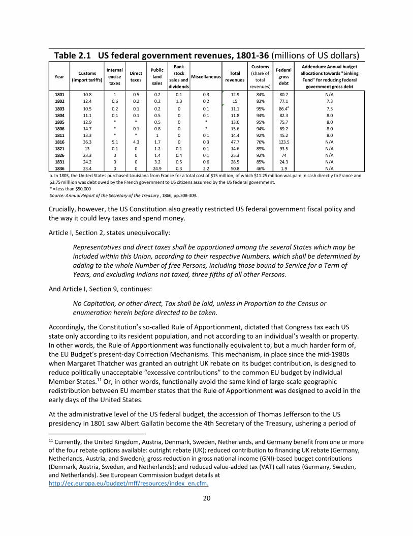
Import tariffs—which had the political benefits of mostly affecting the more affluent consumers as well as protecting domestic industry from overseas competition—were by far the most dominant source of federal revenue in the early US republic. In many fiscal years, they accounted for over 90 percent of all revenues (table 2.1). While initially tariff levels were related to the need for revenues for the “sinking fund”10 to pay down war‐related federal government debts, over time differing regional political coalitions in Congress pushed the average US tariff levels up to shield various domestic industries from foreign competition. This culminated in the 1828 Tariffs of Abominations at an average level of 41 percent across dutiable articles, before protection levels were gradually reduced starting in 1833 (Studenski and Krooss 1952, 98f). 

Rapidly rising tariff revenue and booming income from federal land sales saw federal government surpluses accumulate and allowed the Andrew Jackson administration to completely retire the outstanding gross federal government debt by 1834 (table 2.1).  

                                                            9 Article IV, Section 3, Clause 2.  10 The federal government “sinking fund” for debts saw a predetermined level of revenue set aside ahead of all other expenditure items and earmarked towards paying down the federal debt. In years of federal government surpluses, this guaranteed a reduction in gross outstanding debts, while in overall deficit years total outstanding debts might not decrease. 

20  

 

Crucially, however, the US Constitution also greatly restricted US federal government fiscal policy and the way it could levy taxes and spend money.  

Article I, Section 2, states unequivocally: 

Representatives and direct taxes shall be apportioned among the several States which may be included within this Union, according to their respective Numbers, which shall be determined by adding to the whole Number of free Persons, including those bound to Service for a Term of Years, and excluding Indians not taxed, three fifths of all other Persons. 

And Article I, Section 9, continues: 

No Capitation, or other direct, Tax shall be laid, unless in Proportion to the Census or enumeration herein before directed to be taken. 

Accordingly, the Constitution’s so‐called Rule of Apportionment, dictated that Congress tax each US state only according to its resident population, and not according to an individual’s wealth or property. In other words, the Rule of Apportionment was functionally equivalent to, but a much harder form of, the EU Budget’s present‐day Correction Mechanisms. This mechanism, in place since the mid‐1980s when Margaret Thatcher was granted an outright UK rebate on its budget contribution, is designed to reduce politically unacceptable “excessive contributions” to the common EU budget by individual Member States.11 Or, in other words, functionally avoid the same kind of large‐scale geographic redistribution between EU member states that the Rule of Apportionment was designed to avoid in the early days of the United States. 

At the administrative level of the US federal budget, the accession of Thomas Jefferson to the US presidency in 1801 saw Albert Gallatin become the 4th Secretary of the Treasury, ushering a period of 

                                                            11 Currently, the United Kingdom, Austria, Denmark, Sweden, Netherlands, and Germany benefit from one or more of the four rebate options available: outright rebate (UK); reduced contribution to financing UK rebate (Germany, Netherlands, Austria, and Sweden); gross reduction in gross national income (GNI)‐based budget contributions (Denmark, Austria, Sweden, and Netherlands); and reduced value‐added tax (VAT) call rates (Germany, Sweden, and Netherlands). See European Commission budget details at http://ec.europa.eu/budget/mff/resources/index_en.cfm.  

YearCustoms 

(import tariffs)

Internal 

excise 

taxes

Direct 

taxes

Public 

land 

sales

Bank 

stock 

sales and 

dividends

MiscellaneousTotal 

revenues

Customs 

(share of 

total 

revenues)

Federal 

gross 

debt

Addendum: Annual budget 

allocations towards "Sinking 

Fund" for reducing federal 

government gross debt

1801 10.8 1 0.5 0.2 0.1 0.3 12.9 84% 80.7 N/A

1802 12.4 0.6 0.2 0.2 1.3 0.2 15 83% 77.1 7.3

1803 10.5 0.2 0.1 0.2 0 0.1 11.1 95% 86.4a

7.3

1804 11.1 0.1 0.1 0.5 0 0.1 11.8 94% 82.3 8.0

1805 12.9 * * 0.5 0 * 13.6 95% 75.7 8.0

1806 14.7 * 0.1 0.8 0 * 15.6 94% 69.2 8.0

1811 13.3 * * 1 0 0.1 14.4 92% 45.2 8.0

1816 36.3 5.1 4.3 1.7 0 0.3 47.7 76% 123.5 N/A

1821 13 0.1 0 1.2 0.1 0.1 14.6 89% 93.5 N/A

1826 23.3 0 0 1.4 0.4 0.1 25.3 92% 74 N/A

1831 24.2 0 0 3.2 0.5 0.6 28.5 85% 24.3 N/A

1836 23.4 0 0 24.9 0.3 2.2 50.8 46% 1.9 N/A

* = less than $50,000

Source: Annual Report of the Secretary of the Treasury , 1866, pp.308‐309.

Table 2.1   US federal government revenues, 1801‐36 (millions of US dollars)

a. In 1803, the United States purchased Louisiana from France for a total cost of $15 million, of which $11.25 million was paid in cash directly to France and 

$3.75 milllion was debt owed by the French government to US citizens assumed by the US federal government.

21  

rising congressional control over US Treasury operations, following the rapid and necessarily opportunistic early expansion under Hamilton (Powell 1939, 177ff). 

As a former congressional critic of Hamilton’s policies to secure a strong and independent US Treasury, Gallatin helped reassert direct congressional control over the federal government budget. He replaced Hamilton’s preference for lump‐sum appropriations (providing the Secretary of the Treasury with wide discretion on where money was ultimately spent) with a system of specific appropriations with detailed congressional designation of where and towards what ends federal funds were spent, and explicitly forbade the transfer of funds to any subject other than the one originally appropriated by Congress, even within the government department. Annual State of the Government Finances reports had to be submitted to Congress from 1800 onwards, and Gallatin implemented that the legislative branch kept full control of the federal government’s ability to borrow by having Congress specify the terms and amounts of each bond or loan. Gallatin’s reforms, which put Congress firmly in charge of the entire federal government budget process of appropriations, revenue collection, and debt lasted well into the 20th century and was not materially reformed until World War I. 

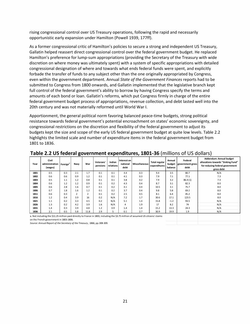
Apportionment, the general political norm favoring balanced peace‐time budgets, strong political resistance towards federal government’s potential encroachment on states’ economic sovereignty, and congressional restrictions on the discretion and flexibility of the federal government to adjust its budgets kept the size and scope of the early US federal government budget at quite low levels. Table 2.2 highlights the limited scale and number of expenditure items in the federal government budget from 1801 to 1836. 

 

 

   

Year

Civil 

administration 

(wages)Foreign

a Navy WarVeterans' 

pensions

Indian 

relations

Interest on 

national 

debt

MiscellaneousTotal regular 

expenditures

Annual 

budget 

balance

Federal 

government gross 

debt

Addendum: Annual budget 

allocations towards "Sinking Fund" 

for reducing federal government 

gross debt

1801 0.5 0.3 2.1 1.7 0.1 0.1 4.4 0.3 9.4 3.5 80.7 N/A

1802 0.6 0.6 0.9 1.2 0.1 0.1 4.1 0.3 7.9 7.1 77.1 7.3

1803 0.5 1.1 1.2 0.8 0.1 0.1 3.8 0.2 7.9 3.2 86.4 (1) 7.3

1804 0.6 1.2 1.2 0.9 0.1 0.2 4.3 0.4 8.7 3.1 82.3 8.0

1805 0.6 2.8 1.6 0.7 0.1 0.2 4.1 0.4 10.5 3.1 75.7 8.0

1806 0.7 1.8 1.6 1.2 0.1 0.2 3.7 0.4 9.8 5.8 69.2 8.0

1811 0.6 0.3 2 2 0.1 0.2 2.5 0.5 8.1 6.4 45.2 8.0

1816 1.2 0.4 3.9 16 0.2 N/A 7.2 1.7 30.6 17.1 123.5 8.0

1821 1.1 0.2 3.3 4.5 0.2 N/A 5.1 1.4 15.8 ‐1.2 93.5 N/A

1826 1.3 0.2 4.2 3.9 1.6 N/A 4 1.9 17 8.2 74 N/A

1831 1.4 0.3 3.9 4.8 1.2 0.9 1.4 1.4 15.2 13.3 24.3 N/A

1836 2.1 0.5 5.8 11.8 2.9 5 0.1 2.7 30.9 19.9 1.9 N/A

Source: Annual Report of the Secretary of the Treasury , 1866, pp.308‐309.

a. Not including the $11.25 million paid directly to France in 1803, including the $3.75 million of assumed US citizens' claims 

on the French government in 1803‐1806.

Table 2.2 US federal government expenditures, 1801‐36 (millions of US dollars)

22  

2.2 Federal Surpluses and State Defaults in the First Half of the 19th Century 

In response to rising surpluses beginning in the late 1820s, political pressures gradually built for the federal government to expand funding of so‐called internal improvements, e.g., domestic infrastructure.12 A debate reminiscent of the original dispute over the role of US federal debt between Hamilton and Jefferson, however, greatly affected congressional thinking and federal policy. Adherents of the Hamiltonian tradition felt the federal government, under the Constitution’s “general welfare clause,” ought to play a leading role in contributing to national welfare and enhancing economic opportunities through internal improvements. Jeffersonians, on the other hand, feared that a proactive federal government increasingly responsible for national infrastructure improvements would become all‐powerful and states’ autonomy would be undermined. Instead the states ought to take the lead in providing better public infrastructure, while the federal government would only be constitutionally permitted to do so in the newly organized Western territories not yet fully incorporated into the federal structure through statehood. President Andrew Jackson (1829–37) belonged to the latter school of thought and repeatedly vetoed large‐scale federal government sponsored infrastructure projects, though still oversaw a sizable increase in federal government spending on internal improvements in the West.13 

Federal government surpluses, however, continued to build in the early 1830s and led to several attempts at disposing of it. President Jackson’s Treasury Secretary Levi Woodbury proposed in 1835 the first US federal government “rainy day fund” to accumulate and carefully invest surpluses “as a provident fund to be ready to meet any contingencies attending the great reduction contemplated in our revenues hereafter.”14 Congress ignored the proposal and instead listened to pleas from the increasingly indebted US states to distribute federal surpluses among them. In 1836 Congress proceeded to distribute all federal surpluses above $5 million to the states in the form of interest‐free loans, enabling President Jackson to continue to claim that the fiscal transfers were not a gift. In fact, the short‐lived 1836 federal surplus transfer to the states was the forerunner of later periods’ important federal government grants‐in‐aid to states. (The transfer had ended when the financial panic of 1837 brought the United States deep recession and much reduced tariff and land sale revenues for the federal government.) 

The generally very conservative federal government fiscal policy of the 1820s and early 1830s, which saw the entire federal government debt retired and severely restricted federal government investments in improving the national infrastructure, did not, however, prevent (and likely contributed to) fiscal excesses elsewhere in the US general government. In complete contrast to the federal government, the US states and later municipalities increased their debts dramatically during this period to fund the kind of large‐scale infrastructure projects that the federal government refrained from financing for political reasons. As a result, while outstanding federal government debt declined rapidly towards zero in the 1820s and early 1830s, US states’ debts (and therefore US general government debts) rose dramatically and by 183815 stood at $175 million, exceeding the highest level of federal government debt recorded at 

                                                            12 The political compromise of 1833 between protectionists and industrialists allowed for only a gradual reduction in protective tariffs, meaning that federal surpluses could not simply be reduced by lowering federal government revenues from tariffs. 13 Studenski and Krooss (1952, 101) lists federal government infrastructure and public works projects worth more than $25 million between 1829 and 1836, financing roads, canals, military infrastructure, rivers, harbors, lighthouses, and other public buildings. 14 US Treasury, Annual Report of the Secretary of the Treasury, 1835. 15 Comprehensive data for US states’ debts are not available before 1830, and even afterwards are available only for select years. 

23  

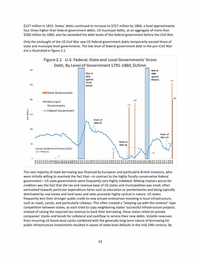
$127 million in 1815. States’ debts continued to increase to $257 million by 1860, a level approximately four times higher than federal government debts. US municipal debts, at an aggregate of more than $200 million by 1860, also far exceeded the debt levels of the federal government before the Civil War. 

Only the onslaught of the US Civil War saw US federal government debts temporarily exceed those of state and municipal level governments. The low level of federal government debt in the pre–Civil War era is illustrated in figure 2.1. 

 

The vast majority of state borrowing was financed by European and particularly British investors, who were initially willing to overlook the fact that—in contrast to the highly fiscally conservative federal government—US state governments were frequently very highly indebted. Making matters worse for creditors was the fact that the tax and revenue base of US states and municipalities was small, often earmarked towards particular expenditure items such as education or penitentiaries and being typically dominated by real estate and land taxes and sales proceeds highly cyclical in nature. US states frequently lent their stronger public credit to new private enterprises investing in local infrastructure, such as roads, canals, and particularly railways. This often created a “keeping‐up‐with‐the‐Joneses” type competition between states, as each tried to copy neighboring states’ successful infrastructure projects. Instead of raising the required tax revenue to back their borrowing, these states relied on private companies’ stocks and bonds for collateral and cashflow to service their new debts. Volatile revenues from recurring US boom‐bust cycles combined with the generally long‐term nature of borrowing for public infrastructure investments resulted in waves of state‐level defaults in the mid‐19th century. By 

24  

1841, eight US states16 and the then territory of Florida (a third of the total of 28 states and territories at the time) had defaulted on their debt obligations. 

In contrast to the Hamiltonian takeover of war‐related state debts after the War of Independence in 1790 and War of 1812 in 1815, there was no federal government bailout in the early 1840s, despite defaulting states’ request to Congress to absorb their debts, despite the evident fiscal capacity of the federal government to do so, and despite the presence of significant cross‐state financial contagion in the state bond markets, as bond prices for even financially sound states fell, and the US federal government itself was cut off from European financing in 1842.  

Congress, however, was politically able to reject the petition for a federal bailout of the affected states for several reasons. First, states incurred debts largely to finance infrastructure projects to strengthen their local economies (and often to compete with successfully industrializing neighboring states) and not provide national public goods, which the federal government was constitutionally required to do when undertaking projects at the time. Second, the defaulted bonds were overwhelmingly held by foreign creditors and did not constitute a large part of the US domestic banking portfolio, so the defaults themselves had limited direct contagion effects on the US financial system and caused little financial pain for domestic savers. Third, the financially solid US states outnumbered defaulting states.17 And, finally, the US economy had reached a stage in development where it could longer be denied continued access to foreign (e.g., European) capital. Imposing losses on foreign creditors was therefore less risky than before. 

Eventually, following defaults in the form of debt repayment moratoria, most states repaid most or all of their debt as a condition for returning to private financial markets.18 The rejection of debt assumption by the defaulting states established a strong political “no bailout” norm on the part of the federal government.19 This norm is neither a legal statute in the US Constitution nor even a clause in federal law. Nevertheless, it has proven politically powerful, as no state bailout request has been accepted since the early 19th century.20 

The fiscal sovereignty of US states was an indirect outcome of the “no bailout” norm—established and in some ways imposed upon some US states by (the majority of) other states—and the unwillingness of the federal government to carry out many parts of national infrastructure construction and rejection of any federal government bailouts. This set a very potent political precedent in the fiscal interaction between US states and the federal government. Subsequently, during the 1840s and 1850s, states began their own procedures to adopt balanced budget amendments to their state constitutions or institute other legal provisions in state law demanding state governments run (at least partly) balanced budgets. Even financially solid states that had not defaulted adopted such measures, which continued 

                                                            16 These were Louisiana, Maryland, Illinois, Arkansas, Michigan, Alabama, Pennsylvania, Mississippi, and Indiana. 17 Wallis, Sylla, and Grinath (2004) shows how seven US states had virtually no state debts in 1841, while most other nondefaulting states had per capita debt levels far below those of the defaulting states.  18 By 1848, only Arkansas had not yet either restructured or resumed payments on its bonds (Wallis, Sylla, and Grinath 2004, table 2). 19 Substantial US state government default and debt repudiation, however, took place later among the Southern former Confederate States, as these were reintegrated into the United States following the end of the Civil War in 1865. 20 This applies only to US states, while arguably an exception was made in the 1995 federal government bailout of the District of Columbia. In this case, Congress did indeed in true “Troika fashion” take control of the District’s finances, injected federal government funds, and managed the budget for four years through the District of Columbia Financial Control Board. This was possible because of a special clause in the Constitution giving Congress authority over the administration of the District—authority that does not extend to the “sovereign” US states. 

25  

over the course of subsequent decades. By the time of the US Civil War essentially all states had adopted some sort of balanced budget restrictions on state government finances. US states’ balanced budget clauses were therefore not a coordinated federal top‐down policy initiative but the outcome of internal state “domestic politics” following the 1840s debt crisis. 

Constitutional revisions in many US states in the 1840s and 1850s, in addition to various versions of balanced budget provisions, also saw the introduction of other legal features aimed at reducing excessive borrowing and strengthening the public’s control over state government finances. Various fiscal and administrative officeholders—such as state comptrollers, treasurers, superintendents of public works—became directly elected with fixed terms, property taxes (often the most important state revenue generator and favorite source of emergency revenues to stave off bond defaults in cash flow crises) could be levied only according to uniform rules, appropriations had to be specific rather than lumpsum, and new tax laws had to specify the purpose for which the new revenue was to be raised for.  

The latter provisions earmarking tax revenues towards specific government tasks proved to be a necessary evil. Earmarking naturally reduced state governmental discretion to allocate and spend public resources, thereby facilitating the public’s willingness to be taxed towards providing clearly identifiable government tasks and services. As such, revenue earmarking was frequently a political necessity for state governments to raise any kind of tax‐based revenues towards services provision. At the same time, however, the resulting balkanization of the overall budget process and establishment of numerous special budgetary funds for the provision of only specific governmental tasks and services (such as education, prisons, mental health, old age and disabled care) made overall flexible and stable state government financing impossible. Combined with the control party machines frequently acquired over directly elected state commissioners and administrative officials, the fundamental lack of public confidence in sound government decision making for the public good that revenue earmarking represents put 19th century US state governments on a path to frequently dysfunctional fiscal and budget processes not rectified until the dramatic changes in state and federal government relations during the 1930s New Deal.  

3 Consolidating America’s Fiscal Union from the Civil War to World War I 

3.1 Expanding the Federal Government to Finance the Civil War  

 When the US Civil War broke out in 1861, the US federal government’s capacity to finance an all‐out effort to secure victory was completely inadequate. The US fiscal union was at the time a fair weather fiscal union without the features to withstand the shock of total war—not unlike the early euro monetary institutional design, which was revealed after the euro area crisis began in 2010 to be defective without a common bailout fund or integrated uniform banking supervision. Important basic elements of what later became the modern American fiscal union were consequently adopted out of necessity to finance the war effort. Many of these new measures, including federal income taxation, were however abandoned after the war, as the federal government’s fiscal emergency ended and traditional political pressures to focus on limited central government and debt repayment regained political supremacy. 

Even in the more industrialized North the US economy remained mostly agricultural and excess private savings were not easily available to enable the federal government to quickly borrow large sums of money to finance the war effort. Greatly aggravating the dire federal government financial situation at the outset of the war was the inadequate government revenue collection system and, based on the erroneously optimistic view that the war would be over soon, congressional unwillingness to quickly enact new taxes to pay for the war. Prewar federal government revenues largely consisted of import 

26  

duties, sales of federal land, and miscellaneous other sources, all of which were decimated by the outbreak of the Civil War. Domestic sales taxes had not been leveled in the United States since the early 1820s, and widespread direct income taxation had never been attempted.  

As a result, the federal government—despite its borrowing difficulties—was initially left with no choice other than to rely very heavily on borrowed funds to finance its quickly expanding war effort. Only as the war dragged on was federal government borrowing complemented by rising tax revenues and new issuance of paper money to finance military operations. 

Numerous obstacles hampered federal government loan financing of its military expenditures. Borrowing was administratively impeded by the constitutional need to secure congressional approval for the detailed terms (principal, maturity, interest rate, and other terms) of each loan, rendering nimble Treasury debt operations in volatile loan markets impossible. The federal government had no central bank and hence did not control its own fiscal agent. Having maintained low levels of federal debt for many years meant that it retained limited expertise in raising large loans from the more than 1,500 state banks in the United States.21 The lack of a US central bank and official single consolidated paper currency in 1861, moreover, meant that the United States at the time operated a de facto dual currency system of gold and private fiat money. Total outstanding American currency at the outset of the Civil War, estimated by Studenski and Krooss (1952) at $450 million, was a mixture of $250 million in gold and $200 million in privately issued paper currency of varying credibility. 

Early war financing efforts saw the federal government show great ingenuity in raising funds, including short‐ and long‐term bonds, noninterest bearing Treasury demand notes, temporary deposit notes, other certificates of federal government indebtedness, and the issuance and circulation of the first federal government‐backed paper currency. To finance the ongoing war effort, Congress over time greatly expanded other federal government revenue sources, especially adding new tax‐based items. Import tariffs were raised, direct taxes were levied on the states, new federal personal income taxes were adopted, as were numerous manufacturing sales and licensing taxes, and revenue was raised from the sales of public lands, including over the course of the war from confiscated previous Confederate property (e.g., quite literally the sales of war booty). To raise funds for the war effort, the federal government introduced three main fiscal policy innovations during the Civil War: paper money (greenbacks), a nationally chartered banking system, and federal sales and income taxes. 

Greenbacks. Early battlefield reversals for the North in 1861–62, combined with the federal government’s enormous increase in expenditures and borrowing, led to a general loss of confidence and associated private investor flight to quality and hoarding of gold. Thus, to protect their dwindling reserves both private banks and the federal government suspended gold payments/conversions in late December 1861.22 In the resulting acute financial squeeze faced by the US Treasury in early 1862, Congress with the Legal Tender Act of February 1862 for the first time approved the issuance of federal 

                                                            21 At the outset of the Civil War, the United States had neither a central bank nor a national banking system, as the federal government did not issue banking licenses covering the entire country. The private US banking system at the time was hence greatly balkanized, and banks were by definition local and chartered only by the state in which they resided. New York, due to its close ties to the European financial markets and important role in international trade (and hence import tariff payments to the federal government in gold), was already established as the premier US financial center. 22 Even after the banks and federal government suspended gold payments, private businesses still needed gold to pay international loans as well as import duties to the federal government (and the federal government needed gold to pay interests on its bonds). Consequently, a liquid market for gold traded in paper money was established in New York in early 1862 (Studenski and Krooss 1952, 143). 

27  

government non‐interest‐bearing Treasury notes not redeemable in gold (e.g., paper money issued on solely the full faith and credit of the United States government). The Legal Tender Act authorized the issuance of $150 million of such notes, which came to be called “greenbacks,” and made them legal tender for all private and public transactions, except payment of import tariff duties and interest on the federal debt. Despite congressional protestations that the first greenback issuance would also be the last and in the face of continuing difficulties for the US Treasury in financing the war, the first issuance of greenbacks was followed by another $150 million in July 1862 and a third issue of $150 million in January 1863. 

National Banking Charter. Following the general political adherence to laissez faire principles and limited federal government, no nationally chartered banks existed at the beginning of the war and vigorous resistance from the banking sector itself (which preferred operating under the perceived less stringent state banking charters) meant that the National Banking Act was passed by Congress only in February 1863. The congressional intent with the Act was threefold: first, as the importance of the federal government “greenback notes” issuance was not yet evident, to create a more uniform national paper currency backed by nationally chartered banks’ gold (as opposed to the various paper money issuances of varying quality by state chartered banks); second, to provide for natural private market demand for federal government debt from such banks;23 and third, through federal oversight, to prevent repeated boom‐bust banking cycles of overexpansion and then rapid depreciation of paper money issuance. The Act enabled nationally chartered banks to issue paper money backed by the US Treasury itself and uniformly printed by the federal government. Such issuance could take place in proportion to the nationally chartered bank’s capital overseen by the newly created Office of the Comptroller of the Currency inside the US Treasury. Initially, however, interest among state chartered banks (and entrepreneurs) for a federal government national banking license was limited. Congress consequently passed a first 2 percent and by 1866 10 percent tax on state chartered banks’ issued notes, greatly favoring nationally chartered banks and effectively driving state banks out of the business of issuing their own notes. Hence the National Banking Act of 1863 helped establish a more uniform US currency and created the distinction between national and state chartered banks in the United States still in existence today. 

Federal Taxes. In the face of persistent Treasury difficulties in raising funds for the war effort, Congress belatedly in July 1862 passed a new and—by federal US government standards—unprecedented comprehensive set of new taxes. These included internal duties (e.g., sin‐type luxury taxes) on spirits, tobacco, auction sales, sugar, and many other products; license taxes on various retailers; stamp duties on legal documents; ad valorem or fixed taxes on all manufacturing articles; 1.5 to 3 percent sales taxes on gross receipts from railroads, ferryboats, steamships, toll bridges, and advertising; to protect domestic manufacturing a further increase of import duties (still payable in gold); a slightly progressive income tax of 3 percent above incomes over $600 and 5 percent on those above $10,000; and finally an inheritance tax on values above $1,000. 

In its need to raise revenues Congress evidently took full advantage of the American public’s war‐induced increased willingness to pay taxes and legislated a very broad tax burden across as many economic sectors and individuals as possible. This had obvious advantages for revenue generation but created great administrative collection difficulties. The newly created Commissioner of Internal 

                                                            23 The Treasury could deposit its public funds in any nationally chartered bank (thereby increasing its banking reserves facilitating additional lending), provided these funds were secured by the bank purchasing and depositing US Treasury bonds in return. 

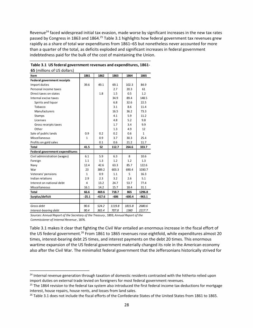
28  

Revenue24 faced widespread initial tax evasion, made worse by significant increases in the new tax rates passed by Congress in 1863 and 1864.25 Table 3.1 highlights how federal government tax revenues grew rapidly as a share of total war expenditures from 1861–65 but nonetheless never accounted for more than a quarter of the total, as deficits exploded and significant increases in federal government indebtedness paid for the bulk of the cost of maintaining the Union. 

 

Table 3.1 makes it clear that fighting the Civil War entailed an enormous increase in the fiscal effort of the US federal government.26 From 1861 to 1865 revenues rose eightfold, while expenditures almost 20 times, interest‐bearing debt 25 times, and interest payments on the debt 20 times. This enormous wartime expansion of the US federal government materially changed its role in the American economy also after the Civil War. The minimalist federal government that the Jeffersonians historically strived for 

                                                            24 Internal revenue generation through taxation of domestic residents contrasted with the hitherto relied upon import duties on external trade levied on foreigners for most federal government revenues. 25 The 1864 revision to the federal tax system also introduced the first federal income tax deductions for mortgage interest, house repairs, house rents, and losses from land sales. 26 Table 3.1 does not include the fiscal efforts of the Confederate States of the United States from 1861 to 1865. 

Item 1861 1862 1863 1864 1865

Federal government receipts

Import duties 39.6 49.1 69.1 102.3 84.9

Personal income taxes 2.7 20.3 61

Direct taxes on states 1.8 1.5 0.5 1.2

Internal excise taxes 34.9 89.4 148.5

Spirits and liquor 6.8 32.6 22.5

Tobacco 3.1 8.6 11.4

Manufacturers 16.5 36.2 73.3

Stamps 4.1 5.9 11.2

Licenses 4.8 5.2 9.8

Gross receipts taxes 1.7 3.4 9.9

Other 1.3 4.9 12

Sale of public lands 0.9 0.2 0.2 0.6 1

Miscellaneous 1 0.9 3.7 30.3 25.4

Profits on gold sales 0.1 0.6 21.2 11.7

Total  41.5 52 112.7 264.6 333.7

Federal government expenditures

Civil administration (wages) 6.1 5.9 6.3 8 10.6

Foreign 1.1 1.3 1.2 1.2 1.3

Navy 12.4 42.6 63.3 85.7 122.6

War 23 389.2 603.3 690.4 1030.7

Veterans' pensions 1 0.9 1.1 5 16.3

Indian relations 2.9 2.3 3.2 2.6 5.1

Interest on national debt 4 13.2 24.7 53.7 77.4

Miscellaneous 16.1 14.2 15.7 18.4 31.1

Total  66.6 469.6 718.7 865 1296.8

Surplus/deficit ‐25.1 ‐417.6 ‐606 ‐600.4 ‐963.1

Gross debt 90.6 524.2 1119.8 1815.8 2680.6

Interest‐bearing debt 90.4 365.4 707.8 1360 2217.7

Table 3.1  US federal government revenues and expenditures, 1861‐

65 (millions of US dollars)

Sources: Annual Report of the Secretary of the Treasury , 1893; Annual Report of the 

Commissioner of Internal Revenue , 1876.

29  

was no longer a possibility, as the federal government’s fiscal (e.g., revenue, expenditure, and debt management) policies now affected almost all American businesses and individuals.  

Crucially, this government expansion was possible only due to the war‐time emergency, rendering the American public willing in the name of the survival of the Union to accept previously unacceptable centralization and expansion of federal government power. Even though many of the war‐time measures were (temporarily) repealed after the end of the Civil War, the war‐time (e.g., period of existential crisis) driven expansion of the US fiscal union shares many of the similarities with the historical crisis driver of European integration and not least recent years’ developments in the European Union and the euro area in particular. The creation of the European Financial Stability Facility (EFSF), later the European Stability Mechanism (ESM), and the European banking union after 2010 would have been impossible without the imperative of addressing the euro area sovereign debt crisis. But similarly, hardly any Americans in the late 1850s could have imagined that a federal government income tax or nationally chartered banks would come into existence just a few years later during the Civil War. Indeed, Jean Monnet’s famous quote, “Europe will be forged in crises, and will be the sum of the solutions adopted for those crises,” would aptly describe the historical development of the US fiscal union, too. 

3.2 Temporary Retrenchment of the Federal Government after the Civil War 

The end of the Civil War invariably changed the political balance in the United States, as the victorious Northern industrial states with their affluent and politically agile class of industrialists rose to unprecedented political dominance. The Southern rural aristocracy had been destroyed in the war, and Southern lower‐income groups were temporarily disenfranchised during the Northern occupation and Southern reconstruction, while the poorer Western states were not yet numerous enough to challenge the Northern political supremacy. This new political reality had dramatic effects on the operations of the federal government, which during the war years had for the first time grown to be an important factor in the US national economy. Federal government fiscal policy was shaped by Northern industrial and higher income groups’ interests, favoring regressive taxation, protectionism, federal government debt repayment, and an elimination of paper money (e.g., greenbacks) to reduce what had been roaring war‐time price inflation. 

Table 3.2 highlights the evolution of the federal budget from 1866 to 1899. On the expenditure side, military‐related spending was very quickly reduced to almost prewar levels by 1871, while the two biggest expenses became interest on the federal government debt and the accelerating pension payments to Civil War veterans and their dependents. A smaller increase was also witnessed in federal government infrastructure investments on improvements to America’s rivers and harbor facilities. Even in its relatively limited coverage of only war‐related cases from as early as the 1890s, social insurance was the single largest expenditure item on the US federal government budget.  

More dramatically on the revenue side, all income taxation was abandoned by the early 1870s, and inheritance, sales and gross receipts, and almost all manufacturers’ taxes were phased out by 1871. Rising external tariffs once again dominated postwar federal government revenues, though they were now complemented with substantial domestic consumption/sin tax revenue from levies on spirits, liquor, tobacco, and a few other items. Postwar federal government domestic tax revenues were hence almost exclusively regressive in nature. 

Overall fiscal policy was highly conservative. Thanks to the substantial fiscal surpluses until the mid‐1890s, more than two‐thirds of the federal government postwar debt was paid off by 1895, with interest‐bearing debt dropping from $2.3 billion to $716 million. Given that the US economy almost 

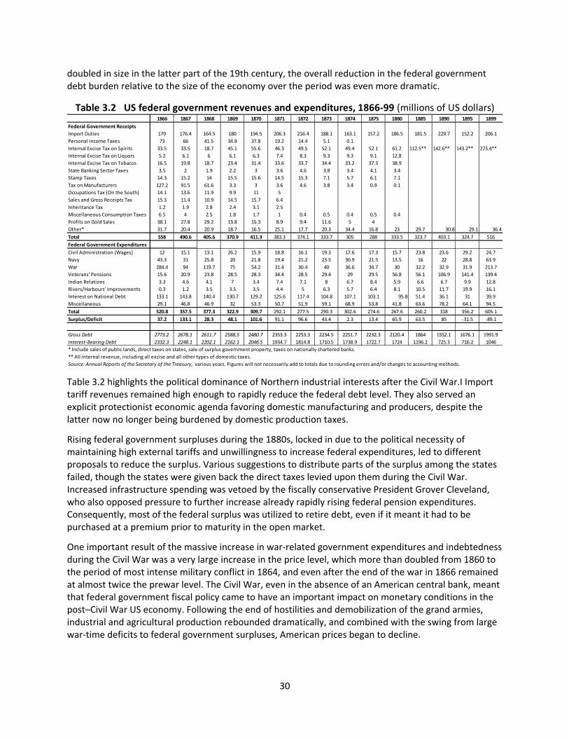
30  

doubled in size in the latter part of the 19th century, the overall reduction in the federal government debt burden relative to the size of the economy over the period was even more dramatic. 

 

Table 3.2 highlights the political dominance of Northern industrial interests after the Civil War.I Import tariff revenues remained high enough to rapidly reduce the federal debt level. They also served an explicit protectionist economic agenda favoring domestic manufacturing and producers, despite the latter now no longer being burdened by domestic production taxes. 

Rising federal government surpluses during the 1880s, locked in due to the political necessity of maintaining high external tariffs and unwillingness to increase federal expenditures, led to different proposals to reduce the surplus. Various suggestions to distribute parts of the surplus among the states failed, though the states were given back the direct taxes levied upon them during the Civil War. Increased infrastructure spending was vetoed by the fiscally conservative President Grover Cleveland, who also opposed pressure to further increase already rapidly rising federal pension expenditures. Consequently, most of the federal surplus was utilized to retire debt, even if it meant it had to be purchased at a premium prior to maturity in the open market. 

One important result of the massive increase in war‐related government expenditures and indebtedness during the Civil War was a very large increase in the price level, which more than doubled from 1860 to the period of most intense military conflict in 1864, and even after the end of the war in 1866 remained at almost twice the prewar level. The Civil War, even in the absence of an American central bank, meant that federal government fiscal policy came to have an important impact on monetary conditions in the post–Civil War US economy. Following the end of hostilities and demobilization of the grand armies, industrial and agricultural production rebounded dramatically, and combined with the swing from large war‐time deficits to federal government surpluses, American prices began to decline.  

1866 1867 1868 1869 1870 1871 1872 1873 1874 1875 1880 1885 1890 1895 1899

Federal Government Receipts

Import Duties 179 176.4 164.5 180 194.5 206.3 216.4 188.1 163.1 157.2 186.5 181.5 229.7 152.2 206.1

Personal Income Taxes 73 66 41.5 34.8 37.8 19.2 14.4 5.1 0.1

Internal Excise Tax on Spirits 33.5 33.5 18.7 45.1 55.6 46.3 49.5 52.1 49.4 52.1 61.2 112.5** 142.6** 143.2** 273.4**

Internal Excise Tax on Liquors 5.2 6.1 6 6.1 6.3 7.4 8.3 9.3 9.3 9.1 12.8

Internal Excise Tax on Tobacco 16.5 19.8 18.7 23.4 31.4 33.6 33.7 34.4 33.2 37.3 38.9

State Banking Sector Taxes 3.5 2 1.9 2.2 3 3.6 4.6 3.8 3.4 4.1 3.4

Stamp Taxes 14.3 15.2 14 15.5 15.6 14.5 15.3 7.1 5.7 6.1 7.1

Tax on Manufacturers 127.2 91.5 61.6 3.3 3 3.6 4.6 3.8 3.4 0.9 0.1

Occupations Tax (On the South) 14.1 13.6 11.9 9.9 11 5

Sales and Gross Receipts Tax 15.3 11.4 10.9 14.5 15.7 6.4

Inheritance Tax 1.2 1.9 2.8 2.4 3.1 2.5

Miscellaneous Consumption Taxes 6.5 4 2.5 1.8 1.7 1 0.4 0.5 0.4 0.5 0.4

Profits on Gold Sales 38.1 27.8 29.2 13.8 15.3 8.9 9.4 11.6 5 4

Other* 31.7 20.4 20.9 18.7 16.5 25.1 17.7 20.3 34.4 16.8 23 29.7 30.8 29.1 36.4

Total  558 490.6 405.6 370.9 411.3 383.3 374.1 333.7 305 288 333.5 323.7 403.1 324.7 516

Federal Government Expenditures

Civil Administration (Wages) 12 15.1 13.1 26.2 15.9 18.8 16.1 19.3 17.6 17.3 15.7 23.8 23.6 29.2 24.7

Navy 43.3 31 25.8 20 21.8 19.4 21.2 23.5 30.9 21.5 13.5 16 22 28.8 63.9

War  284.4 94 119.7 75 54.2 31.4 30.4 40 36.6 34.7 30 32.2 32.9 31.9 213.7

Veterans' Pensions 15.6 20.9 23.8 28.5 28.3 34.4 28.5 29.4 29 29.5 56.8 56.1 106.9 141.4 139.4

Indian Relations 3.3 4.6 4.1 7 3.4 7.4 7.1 8 6.7 8.4 5.9 6.6 6.7 9.9 12.8

Rivers/Harbours' Improvements 0.3 1.2 3.5 3.5 3.5 4.4 5 6.3 5.7 6.4 8.1 10.5 11.7 19.9 16.1

Interest on National Debt 133.1 143.8 140.4 130.7 129.2 125.6 117.4 104.8 107.1 103.1 95.8 51.4 36.1 31 39.9

Miscellaneous 29.1 46.8 46.9 32 53.3 50.7 51.9 59.1 68.9 53.8 41.8 63.6 78.2 64.1 94.5

Total  520.8 357.5 377.3 322.9 309.7 292.1 277.5 290.3 302.6 274.6 267.6 260.2 318 356.2 605.1

Surplus/Deficit 37.2 133.1 28.3 48.1 101.6 91.1 96.6 43.4 2.3 13.4 65.9 63.5 85 ‐31.5 ‐89.1

Gross Debt 2773.2 2678.1 2611.7 2588.5 2480.7 2353.3 2253.3 2234.5 2251.7 2232.3 2120.4 1864 1552.1 1676.1 1991.9

Interest‐Bearing Debt 2332.3 2248.1 2202.1 2162.1 2046.5 1934.7 1814.8 1710.5 1738.9 1722.7 1724 1196.2 725.3 716.2 1046

* Include sales of public lands, direct taxes on states, sale of surplus government property, taxes on nationally chartered banks.

** All internal revenue, including all excise and all other types of domestic taxes.

Source: Annual Reports of the Secretary of the Treasury, various years. Figures will not necessarily add to totals due to rounding errors and/or changes to accounting methods.

Table 3.2   US federal government revenues and expenditures, 1866‐99 (millions of US dollars)

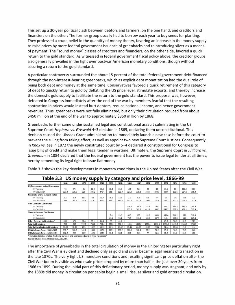
31  

This set up a 30‐year political clash between debtors and farmers, on the one hand, and creditors and financiers on the other. The former group usually had to borrow each year to buy seeds for planting. They professed a crude belief in the quantity of money theory, favoring an increase in the money supply to raise prices by more federal government issuance of greenbacks and reintroducing silver as a means of payment. The “sound money” classes of creditors and financiers, on the other side, favored a quick return to the gold standard. As witnessed in federal government fiscal policy above, the creditor groups also generally prevailed in the fight over postwar American monetary conditions, though without securing a return to the gold standard. 

A particular controversy surrounded the about 15 percent of the total federal government debt financed through the non‐interest‐bearing greenbacks, which as explicit debt monetization had the dual role of being both debt and money at the same time. Conservatives favored a quick retirement of this category of debt to quickly return to gold by deflating the US price level, stimulate exports, and thereby increase the domestic gold supply to facilitate the return to the gold standard. This proposal was, however, defeated in Congress immediately after the end of the war by members fearful that the resulting contraction in prices would instead hurt debtors, reduce national income, and hence government revenues. Thus, greenbacks were not fully eliminated, but only their circulation reduced from about $450 million at the end of the war to approximately $350 million by 1868.  

Greenbacks further came under sustained legal and constitutional assault culminating in the US Supreme Court Hepburn vs. Griswold 4–3 decision in 1869, declaring them unconstitutional. This decision caused the Ulysses Grant administration to immediately launch a new case before the court to prevent the ruling from taking effect, as well as appoint two new Supreme Court Justices. Consequently, in Knox vs. Lee in 1872 the newly constituted court by 5–4 declared it constitutional for Congress to issue bills of credit and make them legal tender in wartime. Ultimately, the Supreme Court in Juilliard vs. Greenman in 1884 declared that the federal government has the power to issue legal tender at all times, hereby cementing its legal right to issue fiat money. 

Table 3.3 shows the key developments in monetary conditions in the United States after the Civil War. 

 

The importance of greenbacks in the total circulation of money in the United States particularly right after the Civil War is evident and declined only as gold and silver became legal means of transaction in the late 1870s. The very tight US monetary conditions and resulting significant price deflation after the Civil War boom is visible as wholesale prices dropped by more than half in the just over 30 years from 1866 to 1899. During the initial part of this deflationary period, money supply was stagnant, and only by the 1880s did money in circulation per capita begin a small rise, as silver and gold entered circulation. 

1866 1868 1870 1872 1874 1876 1878 1880 1882 1884 1890 1892 1894 1896 1899

US Government Notes (Greenbags)

In Treasury 73 27.4 31 11.3 10.6 38.3 25.8 18.8 21.4 28 12 37.1 80 122.4 38.3

In Circulation 327.8 328.6 325 346.2 371.4 331.4 320.9 327.9 325.3 318.7 334.7 309.6 266.6 224.2 308.4

Nationally Chartered Bank Notes

In Treasury 5.5 5.4 11.1 8.6 11.7 16.9 12.8 7.1 6.3 8.8 4.4 5.5 6.6 10.8 3.5

In Circulation 276 294.4 288.6 329 340.3 316.1 311.7 337.4 352.5 330.7 181.6 167.2 200.2 215.2 237.8

Gold Coins and Certificates

In Treasury 126.1 148.5 232.1 348 271.2 131.3 145.3 285.4

In Circulation 233.7 363.3 411.7 505.1 549.7 562.3 497.1 712.4

Silver Dollars and Certificates

In Treasury 6.4 23.5 80.5 130 192.6 350.6 456.8 541.2 562 512.9

In Circulation 21.1 55.1 73.5 133.3 182.8 407.9 545 572.8 538 625.3

Other Currency in Circulation* 69.7 57.2 61.6 63.1 64.4 59 41.4 29.8 58.9 31.9 20.3

Total in Circulation 752 713 717.3 758.2 798.4 789.2 791.2 1205 1480.6 1705.4 2144.3 2371.9 2419.9 2346.9 2744.3

Total Dollars/Capita in Circulation 18.99 18.39 17.5 18.19 18.13 16.12 15.32 19.41 22.37 22.65 22.82 24.44 24.28 21.1 25

US Wholesale Prices (1860 = 100) 190.7 160.2 142.2 138.6 132.8 118.1 101.2 106.8 108.4 99.2 92.2 85.6 78.6 76.3 85.6

UK Wholesale Prices (1860 = 100) 102.9 99.9 96.9 110.3 102.9 96.2 88.1 88.8 85.1 77 72.5 68.9 63.6 61.4 68.8

* Includes state bank notes, fractional currency and unprocessed gold in "gold rush areas"

Source: Studenski and Krooss (1952, 189,239).

Table 3.3   US money supply by category and price level, 1866‐99

32  

The persistent federal government budget surpluses disappeared in the final decade of the 19th century (see table 3.2) due to significant increases in military pension expenditures27 and the elimination of an important import tariff mostly affecting the poor, namely on sugar. The combination of the returning need for additional Treasury fiscal revenue and the accumulating political dissatisfaction with the existing highly regressive federal tax system saw Congress pass a vehemently contested new federal government income tax in 1894.  

The new, limited‐time income tax, as initially envisioned, was to be in effect for five years and apply to both corporations and individuals. It was to be comprehensive in nature and would cover all types of “gains, profits, and income derived from any kind of property, rents, interest, dividends, or salaries, or from any profession, trade, employment, or vocation,”28 also declaring gifts and inheritances as taxable income. It was, however, not a progressive tax and the flat rate was set at 2 percent for annual incomes above $4,000, including both resident and nonresident citizens.29 To promote the sale of Treasury securities, income from such securities was exempted, as were—in a concession to states’ right groups—state and local government employees. 

The constitutionality of the new income tax was immediately challenged. In the famous Pollock vs. Farmer’s Loan and Trust Company case, the Supreme Court in 1895 declared the new federal income tax unconstitutional on the grounds that it was a direct tax and hence subject to the Constitution’s Apportionment Clause. This decision caused widespread political outrage and set in motion the movement that would lead to the passing of the 16th Amendment of the US Constitution annulling the Apportionment Clause some 20 years later. 

The outbreak of and need to finance the Spanish‐American War of 1898 led Congress to reinstate a series of internal indirect excise taxes on various items like tobacco, beer, cosmetics, drugs and chewing gum, as well as levy amusement taxes on theaters and other amusement centers. An inheritance tax on all intergenerational (e.g., not including spouses) estates above $10,000 ranging from 0.75 to 15 percent was also implemented. Fortuitously for the federal government, in 1898 it also received the first significant windfall revenue from its only major involvement in national US infrastructure construction, the construction of transcontinental railroads. That year the Union Pacific and Kansas Pacific Railroads repaid $64 million out of a total of $70 million loan granted,30 greatly helping the war financing effort and highlighting the ability of early federal government loan financing of railroad construction to pay off financially—something that was generally ideologically despised by states’ rights supporters. 

3.3. US Monetary and Fiscal Reforms in the Early 20th Century’s Progressive Era 

As the United States entered the 20th century, the country was growing from an essentially agrarian economy into a world economic power, complete with a limited late‐stage imperialist expansion following the Spanish‐American War. Economic and international political developments alone pushed for a more assertive role for the federal government. At the same time, the inherent financial instability of the country’s still fragile and decentralized banking system, the increasingly politically unacceptable income inequality in the face of a patently regressive tax system, and lack of generally available (other 

                                                            27 The Pension Act of 1890 and subsequent acts saw the number of eligible pensioners (veterans themselves from the Civil War, Indian Wars, and the Mexican War, plus select dependents) almost triple to nearly 1 million. See Studenski and Krooss (1952, 214). 28 See Studenski and Krooss (1952, 233). 29 The 1894 tax for the first time introduced the global tax liability for US citizens still in place today, in contrast to the more widely used territorial tax system. 30 In 1899 Central Pacific Railroad repaid almost $60 million. 

33  

than to war veterans and their relatives) federal government social safety net saw the election of a new category of federalist‐minded presidents—Theodore Roosevelt, William Taft, and Woodrow Wilson. Unlike their post–Civil War predecessors, who generally clung onto the original minimalist vision for the federal government, these men and their administrations favored direct federal government economic interventions in the American economy. The so‐called Progressive Era in the United States during the first two decades of the 20th century saw a significant expansion of federal government powers and the introduction of a number of far‐reaching fiscal and monetary reforms that continue to shape the US economy today. 

The Currency Act of 1900, also known as the Gold Standard Act, established an official American mono‐metallic gold standard with a dollar worth 23.22 grains of pure gold. It replaced what in many ways had been a de facto gold standard in place in the United States since the early 1870s, whereby debt holders could previously demand payment in both gold and silver. Almost all invariably preferred gold, as the law earlier contained an explicit provision that only gold was redeemable for paper money. The subsequent travails for the United States under the Gold Standard are relatively well known in economic history, but the Currency Act of 1900 also contained several other provisions with far‐reaching implications for the stability of the US financial and banking system. 

Minimum capital requirements for nationally chartered banks were reduced to just $25,000 for cities with less than 3,000 inhabitants, and national bank notes could now be issued at 100 percent (previously only 90 percent) of the value of the federal government bonds deposited as security. These provisions increased the fragility of the US banking system by making nationally chartered banks more prone to failures than before, though these were still generally safer than state chartered banks. Studenski and Krooss (1952, 248) note that while 449 out of a total of 8,853 nationally chartered banks failed from 1863–1907 with the loss to creditors (mostly deposits) of about $50 million, more than 2,000 state chartered banks failed during the same period with much higher creditor financial losses. The consistently lax regulation of state banks and state trust companies in the banking sector saw these categories of banks continue to grow as a share of the total US banking system. They were more fragile than the (now less solid) national banks, and due to their frequently highly cyclical and speculative real estate lending and securities’ investments, they suffered repeated liquidity impairments. This instability was greatly aggravated by the fact that the United States still did not possess a central bank onto which private banks’ illiquid assets could be shifted in a panic to avoid a financial collapse. 

Despite the very significant and intended increase—up from $265 million in 1900 to $614 million by 1908—in national‐bank‐issued paper money generated by the Currency Act of 1900, these uniform notes still accounted for only approximately 20 percent of total domestic currency in circulation. US money supply remained highly inelastic, and the requirement that national‐bank‐issued notes be fully backed by banks’ treasury bonds compelled the US Treasury—at a time of rising surpluses and at considerable financial cost—to maintain a sizable outstanding federal government debt to prevent the money supply from contracting. 

Despite half a century of national banking regulation, the United States maintained a desperately fragmented financial system early in the 20th century, which was still dominated by state chartered and regulated banks and trust companies and vulnerable to repeated financial panics (the most severe occurred in 1873, 1893, and 1907). At the same time, as the rapid post–Civil War domestic industrialization and reconstruction came to an end and no longer absorbed all domestic savings and required substantial capital imports, the United States also became an increasingly important international lender. This occurred particularly during periods in which the traditionally financially dominant European powers were at war and hence needed financing for their military campaigns. The 

34  

combination of America’s domestic financial fragility, the US adherence to the gold standard and inelastic domestic money supply, and New York’s increasing importance as an international financial center made the country an increasing source of instability in the international financial system in the early 20th century.  

The last great American financial panic of 1907 prompted Congress to establish the National Monetary Commission in 1908 to study the implementation of a central bank in the United States. A lengthy congressional debate culminated in the 1913 passage of the Federal Reserve Act. The Federal Reserve Act split the United States into (up to) 12 districts, overseen by a Federal Reserve Board located in Washington, DC. Nationally chartered banks were compelled to become members (e.g., shareholders in their new Federal Reserve District Bank), while state chartered banks could only be encouraged to join this new federal government institution. 

The Federal Reserve Act represented major institutional innovation for the United States. It created a lender of last resort, centralized control over the US gold stock, gave the US Treasury a fiscal agent link to the banking system, and provided for the gradual phaseout of bank notes privately issued (by nationally chartered bank).31 The Act created a new and much more elastic central government currency supply and within each district introduced greatly enhanced check clearing opportunities among member banks. It was, however, generally opposed by the American banking sector, which objected to the required use of their capital for purchase of Federal Reserve District Bank stock and (against the interests of their customers) feared a loss of profitability from improved check clearing opportunities. As a result, the Act included several important financial sweeteners for the banking industry, including a (further) general reduction in the bank capital reserve requirement from over 20 percent to an estimated 14 percent, and a new permission for nationally chartered banks to make mortgage loans to farmers.  

The early Federal Reserve System, however, failed to reduce the risks of financial crisis or bank failures in the US financial system to the very low levels hoped for by most of its backers. This was due to a number of politically necessary compromises and an institutional inability to keep up with the rapidly developing US economy. Control over discount rates was diffused to the Federal Reserve Districts, the Federal Reserve Board lacked central instruments of credit control over, for instance, bank reserve requirements, and banking sector membership of the new system was still relatively limited (less than half of all US commercial banking resources and just 37 state chartered banks were members at the beginning), reducing the effectiveness of “moral suasion” by the central bank. The Act did represent a dramatic increase in federal government powers and evidently constituted a huge improvement in the functioning of the American financial system but still decades after its initial implementation was a work in progress, requiring critically important additional components of central banking institutions at a later stage. In that regard, the early decades of today’s American central bank share important similarities with the European System of Central Banks (ESCB). The formation of both central banks represented a crucial step forward to continental economic and monetary integration and centralization. However, in both cases, the initial plans were incomplete and the next big economic downturn following their foundation (the Great Depression in the case of the Federal Reserve and the euro crisis in the case of the European Central Bank (ECB)/ESCB) saw a significant reform and expansion of central powers 

                                                            31 Nationally chartered banks’ paper money could be completely withdrawn only when the often long‐dated federal government bonds containing the specific privilege that banks could use them as deposits with the US Treasury for their own paper money issuances finally expired. A provision inserted into these federal government bonds to entice private banks to buy them, therefore, ended up prolonging the existence of private‐issued paper money in the US banking system for several decades. 

35  

granted to the central banks. Only after 2012 was the ESCB complemented by the Single Supervisory Mechanism (SSM) and the Single Resolution Mechanism (SRM) to enhance and harmonize supervision and resolution of large EU banks. However, the EU banking union continues to lack a fiscal backstop for banking resolution purposes and a fully mutualized deposit insurance system. 

An important outcome of the Progressive Era’s more interventionist presidents was a significant increase in the overall level of US federal government expenditure in the early 20th century. By the time the 16th Amendment, enabling federal income taxes to be collected for the first time, was adopted in 1913, regular peacetime federal government expenditures already exceeded the level of total expenditures during America’s last major war against Spain in 1898. A number of different sources of this expenditure growth can be identified.  

First, President Theodore Roosevelt began the first major push for natural conservation in the United States. Setting aside hundreds of millions of hectares of federally owned land as national parks cost money, as did the establishment of the federal government Forestry Service to manage the new recreational areas for the public.  

Second, the period saw the first sustained example of the federal government making money with strings attached available to state governments through so‐called grants‐in‐aid. The aim was to support the development of the American agricultural sector through the funding of crop experimental stations and agricultural colleges throughout the country. To overcome political concerns over budget redistribution, a single fixed amount of funding—say, $10,000 annually for each state for a given category of agricultural colleges—was typically made available for each state, with additional resources available subject to an objectively valid data ranking, such as the rural population share in a given state. Each state was hence given access to grants‐in‐aid funding, but available resources were to a degree made dependent on the different circumstances in the policy area they were expected to affect across states. Grants‐in‐aid funding came with the additional requirement that state governments match the federal government funds with local resources. This was done to ensure that the local state government, which was expected to administer the federal government’s money, was fully committed to the success of the federally funded program, due to the contribution of its own resources. That the federal government started using grants‐in‐aid funding in the agricultural sector highlights some of the historical parallels between the early development of the US federal government and the EU budget. 

Third, the accelerating development of the American economy required new federal regulations to govern booming interstate commerce, implement new antitrust laws, and ensure uniform national product and services quality in production. These new federal regulatory powers both supplemented and displaced existing state‐level regulations, which was often subject to bitter political and legal disputes. This period saw the establishment of many new federal regulatory agencies, including the Federal Trade Commission, the Bureau of Labor Statistics, the Department of Agriculture’s Phytosanitary Department, the Census Bureau, and numerous others. As economic actors themselves became increasingly national in scope, policing the American economy became the federal government’s responsibility, requiring an expanded budget. 

Fourth, American naval expansion and continued increases in veterans’ pension expenditures increased the overall budget. 

Fifth, the federal government began regularly financing relief for individual Americans subject to natural disasters, such as flooding, hurricanes, or earthquakes.32 The scale and national scope of such natural 

                                                            32 The devastating 1906 quake in San Francisco was an important event in expanding this budget item. 

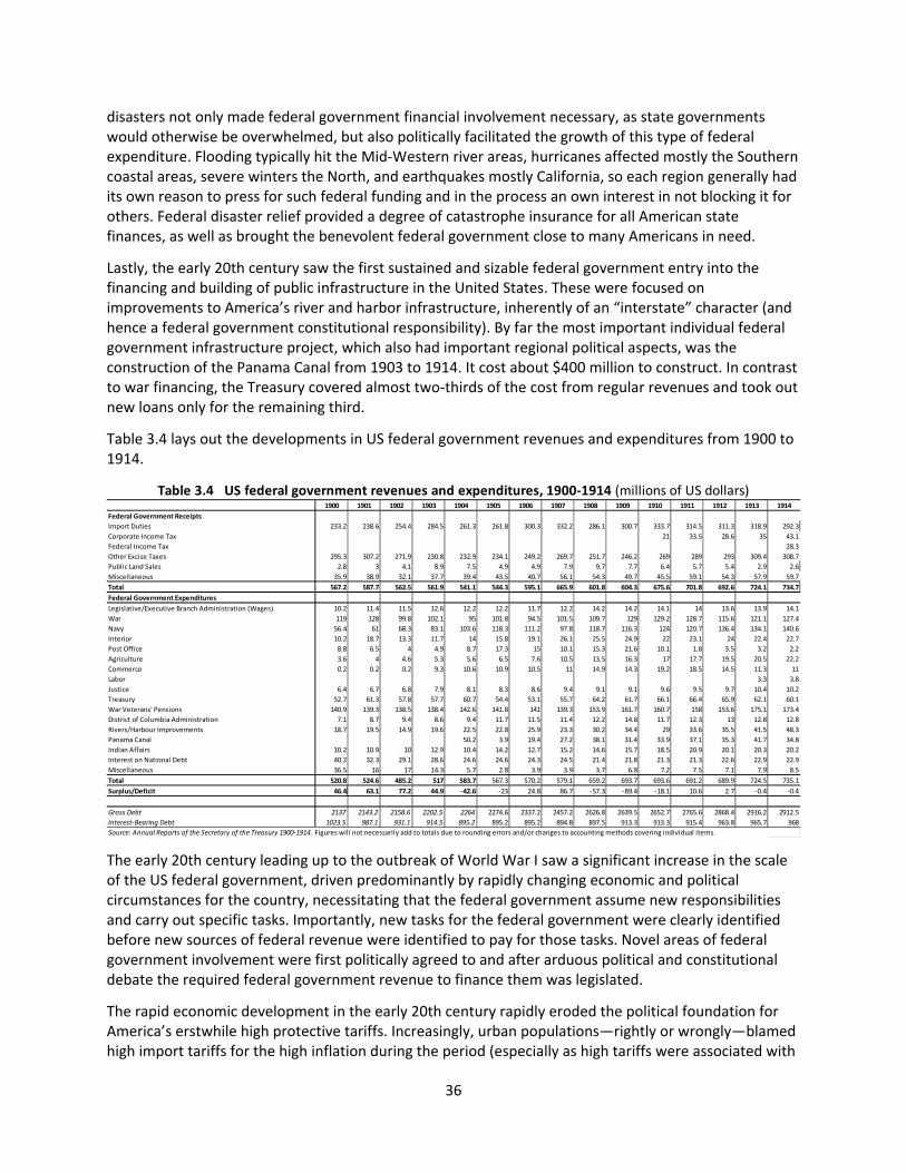
36  

disasters not only made federal government financial involvement necessary, as state governments would otherwise be overwhelmed, but also politically facilitated the growth of this type of federal expenditure. Flooding typically hit the Mid‐Western river areas, hurricanes affected mostly the Southern coastal areas, severe winters the North, and earthquakes mostly California, so each region generally had its own reason to press for such federal funding and in the process an own interest in not blocking it for others. Federal disaster relief provided a degree of catastrophe insurance for all American state finances, as well as brought the benevolent federal government close to many Americans in need. 

Lastly, the early 20th century saw the first sustained and sizable federal government entry into the financing and building of public infrastructure in the United States. These were focused on improvements to America’s river and harbor infrastructure, inherently of an “interstate” character (and hence a federal government constitutional responsibility). By far the most important individual federal government infrastructure project, which also had important regional political aspects, was the construction of the Panama Canal from 1903 to 1914. It cost about $400 million to construct. In contrast to war financing, the Treasury covered almost two‐thirds of the cost from regular revenues and took out new loans only for the remaining third. 

Table 3.4 lays out the developments in US federal government revenues and expenditures from 1900 to 1914. 

 

The early 20th century leading up to the outbreak of World War I saw a significant increase in the scale of the US federal government, driven predominantly by rapidly changing economic and political circumstances for the country, necessitating that the federal government assume new responsibilities and carry out specific tasks. Importantly, new tasks for the federal government were clearly identified before new sources of federal revenue were identified to pay for those tasks. Novel areas of federal government involvement were first politically agreed to and after arduous political and constitutional debate the required federal government revenue to finance them was legislated.  

The rapid economic development in the early 20th century rapidly eroded the political foundation for America’s erstwhile high protective tariffs. Increasingly, urban populations—rightly or wrongly—blamed high import tariffs for the high inflation during the period (especially as high tariffs were associated with 

1900 1901 1902 1903 1904 1905 1906 1907 1908 1909 1910 1911 1912 1913 1914

Federal Government Receipts

Import Duties 233.2 238.6 254.4 284.5 261.3 261.8 300.3 332.2 286.1 300.7 333.7 314.5 311.3 318.9 292.3

Corporate Income Tax 21 33.5 28.6 35 43.1

Federal Income Tax 28.3

Other Excise Taxes 295.3 307.2 271.9 230.8 232.9 234.1 249.2 269.7 251.7 246.2 269 289 293 309.4 308.7

Public Land Sales 2.8 3 4.1 8.9 7.5 4.9 4.9 7.9 9.7 7.7 6.4 5.7 5.4 2.9 2.6

Miscellaneous 35.9 38.9 32.1 37.7 39.4 43.5 40.7 56.1 54.3 49.7 45.5 59.1 54.3 57.9 59.7

Total  567.2 587.7 562.5 561.9 541.1 544.3 595.1 665.9 601.8 604.3 675.6 701.8 692.6 724.1 734.7

Federal Government Expenditures

Legislative/Executive Branch Administration (Wages) 10.2 11.4 11.5 12.6 12.2 12.2 11.7 12.2 14.2 14.2 14.1 14 13.6 13.9 14.1

War  119 128 99.8 102.1 95 101.8 94.5 101.5 109.7 129 129.2 128.7 115.6 121.1 127.4

Navy 56.4 61 68.3 83.1 103.6 118.3 111.2 97.8 118.7 116.3 124 120.7 136.4 134.1 140.6

Interior 10.2 18.7 13.3 11.7 14 15.8 19.1 26.1 25.5 24.9 22 23.1 24 22.4 22.7

Post Office 8.8 6.5 4 4.9 8.7 17.3 15 10.1 15.3 21.6 10.1 1.8 3.5 3.2 2.2

Agriculture 3.6 4 4.6 5.3 5.6 6.5 7.6 10.5 13.5 16.3 17 17.7 19.5 20.5 22.2

Commerce 0.2 0.2 0.2 9.3 10.6 10.9 10.5 11 14.9 14.3 19.2 18.5 14.5 11.3 11

Labor 3.3 3.8

Justice 6.4 6.7 6.8 7.9 8.1 8.3 8.6 9.4 9.1 9.1 9.6 9.5 9.7 10.4 10.2

Treasury 52.7 61.3 57.8 57.7 60.7 54.4 53.1 55.7 64.2 61.7 66.1 66.4 65.9 62.1 60.1

War Veterans' Pensions 140.9 139.3 138.5 138.4 142.6 141.8 141 139.3 153.9 161.7 160.7 158 153.6 175.1 173.4

District of Columbia Administration 7.1 8.7 9.4 8.6 9.4 11.7 11.5 11.4 12.2 14.8 11.7 12.3 13 12.8 12.8

Rivers/Harbour Improvements 18.7 19.5 14.9 19.6 22.5 22.8 25.9 23.3 30.2 34.4 29 33.6 35.5 41.5 48.3

Panama Canal 50.2 3.9 19.4 27.2 38.1 31.4 33.9 37.1 35.3 41.7 34.8

Indian Affairs 10.2 10.9 10 12.9 10.4 14.2 12.7 15.2 14.6 15.7 18.5 20.9 20.1 20.3 20.2

Interest on National Debt 40.2 32.3 29.1 28.6 24.6 24.6 24.3 24.5 21.4 21.8 21.3 21.3 22.6 22.9 22.9

Miscellaneous 36.5 16 17 14.3 5.7 2.8 3.9 3.9 3.7 6.8 7.2 7.5 7.1 7.9 8.5

Total  520.8 524.6 485.2 517 583.7 567.3 570.2 579.1 659.2 693.7 693.6 691.2 689.9 724.5 735.1

Surplus/Deficit 46.4 63.1 77.2 44.9 ‐42.6 ‐23 24.8 86.7 ‐57.3 ‐89.4 ‐18.1 10.6 2.7 ‐0.4 ‐0.4

Gross Debt 2137 2143.2 2158.6 2202.5 2264 2274.6 2337.2 2457.2 2626.8 2639.5 2652.7 2765.6 2868.4 2916.2 2912.5

Interest‐Bearing Debt 1023.5 987.1 931.1 914.5 895.2 895.2 895.2 894.8 897.5 913.3 913.3 915.4 963.8 965.7 968

Source: Annual Reports of the Secretary of the Treasury 1900‐1914.  Figures will not necessarily add to totals due to rounding errors and/or changes to accounting methods covering individual items.

Table 3.4   US federal government revenues and expenditures, 1900‐1914 (millions of US dollars)

37  

the increasingly unpopular presence of domestic monopolies), and increasingly sophisticated American manufacturers clearly realized that high domestic American tariffs reduced the abilities of foreigners to buy their increasingly competitive products due to foreign reciprocal tariffs. As a result Congress, in the 1909 Payne‐Aldrich Tariff Act and in particular the Revenue Act of 1913 (also known as the Underwood Tariff Act), passed a significant one‐quarter reduction in average US import tariff levels and placed important items like steel, raw wool, iron ore, and various agricultural products on the tariff‐free list. 

The reduction in revenues from lower import tariffs, combined with rapidly rising expenditures, compelled Congress to also legislate new sources of federal government revenues. As the 20th century progressed, Congress became more accepting of running peacetime deficits (or at least not sizable annual surpluses aimed at quickly drawing down the federal debt as during the 19th century). This implicitly added a looser fiscal policy as a de facto additional source of federal government resources. 

An amendment to the 1909 Payne‐Aldrich Tariff Act included a new flat rate of 1 percent federal tax on corporate net incomes above $5,000. Crucially, however, the 1909 Act also included the 16th Amendment, repealing the Constitution’s Apportionment Clause and giving Congress the power to tax incomes “from whatever source derived, without apportionment among the several states, and without regard to any census or enumeration.” To the astonishment of congressional conservatives, in just three years the 16th Amendment was passed by the required three‐fourths of the states, becoming part of the US Constitution in February 1913. 

Shortly afterwards, as an amendment to the 1913 Underwood Act, the first and relatively limited US federal income tax was passed. In addition to the earlier 1 percent flat tax on corporate incomes, personal incomes over $3,000 annually ($4,000 for married couples) were taxed by 1 percent, while incomes from $20,000 to $500,000 annually were subject to an additional tax surcharge between one and six percentage points. The first American federal income tax was hence not particularly progressive by later standards, but it was dramatically different from the previous highly regressive federal government nontariff revenue collection system and did for the first time explicitly endorse as its foundation the “ability to pay principle.” In time, given the relatively limited ability of individual state governments in an integrated national economy to pass their own significant income taxes, the 16th Amendment bestowed clear fiscal dominance of the federal government in the United States. 

 4 Creation of America’s Modern Fiscal Union from World War I to the New Deal 

4.1 Shock of World War I to America’s Federal Government 

Just like the extraordinary government efforts to fight and win the Civil War were great centralizing forces in American society and materially strengthened federal government institutions beyond what would have been possible in peace time, the outbreak of World War I in 1914 would in time generate an even larger boost to them. Unlike in the 1860s, when the United States was essentially an agrarian nation, by 1914 it was a major world industrial nation fit to participate in a modern large‐scale military conflict—an ability determined as much by nations’ industrial capacity as their manpower resources.  

Even though the United States participated directly in military operations for only 18 months from 1917 to 1918, the modern industrial warfare type engagement cost the federal government approximately 10 times the cost of fighting for the four years of the Civil War. The requirement for federal government funding was hence far greater, but the much more developed US polity and economy was far better equipped to sustain the increased financial pressures this time. Table 4.1 shows the development of wartime US fiscal policies from 1914 to 1919. 

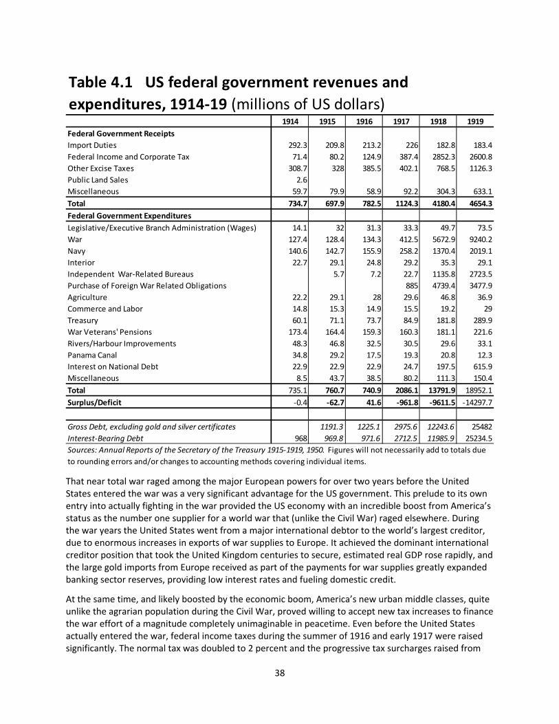
38  

 

That near total war raged among the major European powers for over two years before the United States entered the war was a very significant advantage for the US government. This prelude to its own entry into actually fighting in the war provided the US economy with an incredible boost from America’s status as the number one supplier for a world war that (unlike the Civil War) raged elsewhere. During the war years the United States went from a major international debtor to the world’s largest creditor, due to enormous increases in exports of war supplies to Europe. It achieved the dominant international creditor position that took the United Kingdom centuries to secure, estimated real GDP rose rapidly, and the large gold imports from Europe received as part of the payments for war supplies greatly expanded banking sector reserves, providing low interest rates and fueling domestic credit. 

At the same time, and likely boosted by the economic boom, America’s new urban middle classes, quite unlike the agrarian population during the Civil War, proved willing to accept new tax increases to finance the war effort of a magnitude completely unimaginable in peacetime. Even before the United States actually entered the war, federal income taxes during the summer of 1916 and early 1917 were raised significantly. The normal tax was doubled to 2 percent and the progressive tax surcharges raised from 

1914 1915 1916 1917 1918 1919

Federal Government Receipts

Import Duties 292.3 209.8 213.2 226 182.8 183.4

Federal Income and Corporate Tax 71.4 80.2 124.9 387.4 2852.3 2600.8

Other Excise Taxes 308.7 328 385.5 402.1 768.5 1126.3

Public Land Sales 2.6

Miscellaneous 59.7 79.9 58.9 92.2 304.3 633.1

Total  734.7 697.9 782.5 1124.3 4180.4 4654.3

Federal Government Expenditures

Legislative/Executive Branch Administration (Wages) 14.1 32 31.3 33.3 49.7 73.5

War  127.4 128.4 134.3 412.5 5672.9 9240.2

Navy 140.6 142.7 155.9 258.2 1370.4 2019.1

Interior 22.7 29.1 24.8 29.2 35.3 29.1

Independent  War‐Related Bureaus 5.7 7.2 22.7 1135.8 2723.5

Purchase of Foreign War Related Obligations 885 4739.4 3477.9

Agriculture 22.2 29.1 28 29.6 46.8 36.9

Commerce and Labor 14.8 15.3 14.9 15.5 19.2 29

Treasury 60.1 71.1 73.7 84.9 181.8 289.9

War Veterans' Pensions 173.4 164.4 159.3 160.3 181.1 221.6

Rivers/Harbour Improvements 48.3 46.8 32.5 30.5 29.6 33.1

Panama Canal 34.8 29.2 17.5 19.3 20.8 12.3

Interest on National Debt 22.9 22.9 22.9 24.7 197.5 615.9

Miscellaneous 8.5 43.7 38.5 80.2 111.3 150.4

Total  735.1 760.7 740.9 2086.1 13791.9 18952.1

Surplus/Deficit ‐0.4 ‐62.7 41.6 ‐961.8 ‐9611.5 ‐14297.7

Gross Debt, excluding gold and silver certificates 1191.3 1225.1 2975.6 12243.6 25482

Interest‐Bearing Debt 968 969.8 971.6 2712.5 11985.9 25234.5

Table 4.1   US federal government revenues and 

expenditures, 1914‐19 (millions of US dollars)

Sources: Annual Reports of the Secretary of the Treasury 1915‐1919, 1950. Figures will not necessarily add to totals due 

to rounding errors and/or changes to accounting methods covering individual items.

39  

upto 6 to upto 13 percent for the highest income groups. Corporate income taxes were raised to 8 percent of any business income, and a graduated federal government estate tax was introduced.  

The US entry into World War I in April 1917 saw Congress pass dramatically higher wartime income tax increases, and probably forever changed debates about taxes in America. Following a lengthy debate and more than six months into America’s war effort and with the Treasury in desperate need of more funds, in October 1917 Congress doubled the normal tax again from 2 to 4 percent and increased progressive maximum tax surcharges from 13 to 63 percent. Higher‐income Americans suddenly faced a combined marginal tax rate of 67 percent, a rate well beyond what had previously been considered imaginable. The federal estate tax was raised from 2 to 25 percent. The fact that what proved to be a permanent federal government estate tax was introduced at ultimately very high rates during the war was symptomatic for the manner in which the war effort solidified the federal government’s fiscal dominance. By the early 20th century almost all US states levied their own inheritance taxes, but they were powerless due to wartime necessity to stop the federal government from largely taking over this source of government revenue. 

In mid‐1918, when it became clear that US participation in the war would be prolonged and even more expensive than what had been anticipated, Congress went even further and raised normal income taxes up to 12 percent for 1918 income and raised the progressive surcharge to a maximum of 65 percent, leaving America’s high‐income groups facing a maximum marginal income tax of 77 percent. Facing a top marginal income tax take of more than three‐quarters of affected income in a country where five years earlier such federal government income taxes had been unconstitutional is an astounding change in circumstances for America’s wealthy from 1913 to 1918. And a change imaginable only due to the wartime emergency.  

Despite raising federal income and other taxes to unprecedented levels, war costs rose much faster (see table 4.1). So just like during the Civil War, the federal government had to finance the majority of its expenses through domestic borrowing from the booming American private sector and the American public. The vehicle for doing so, the Treasury’s Liberty Bond Program, started immediately after the US entry into the war in May 1917 and was carried out in an all‐out effort by the US Treasury to entice the US public to purchase the war‐financing bonds. In the words of then US Treasury Secretary William McAdoo (1931, 378): 

We went direct to the people; and that means to everybody—to businessmen, workmen, farmers, bankers, millionaires, schoolteachers, laborers. We capitalized on the profound impulse called patriotism. 

Crucially in the newly emerging highly progressive federal income tax system, Liberty Bonds were exempt from all taxes except estate taxes, making them an essentially unbeatable investment on an after‐tax basis for many Americans and corporations.33 The Liberty Bond campaigns during and immediately after World War I proved extraordinarily successful and amounted to over $19 billion of the total US Treasury net debt of $25.5 billion at its peak in August 1919. Success in reaching small American retail investors was incredible, as Liberty Bonds were sold in almost 80 million individual pieces, of which 40 million were worth less than $50. Studenski and Krooss (1952, 292) cite contemporary estimates that approximately 30 percent of outstanding Liberty Bonds were owned by people with annual income of less than $2,000, which was the federal government tax exemption for a married couple. In other words, 

                                                            33 In early 1918, several additional features were added to improve investor appetite for Liberty Bonds, including making them government receivables when paying estate taxes and instituting a new sinking fund in which the Treasury would repurchase up to 5 percent of each Liberty Bond issue to support prices. 

40  

while the tax‐exempt status of Liberty Bonds surely enticed a very large number of wealthier Americans to invest in this asset class, a numerically much larger group of lower‐income Americans did so without receiving much or any direct financial benefit from their investments. The patriotic feelings stirred up by the war were enough for them to part with their money to support the federal government’s war effort. 

The astonishing success of the Liberty Bond program of war financing during World War I had a profound impact on the development of the American financial system, as it familiarized an entire generation of professional and retail investors with bonds as an asset class. After the war ended, the corporate bond market in the United States had uniquely good growth prospects as an alternative to commercial bank loans for businesses seeking additional capital. The historical link between the American federal government’s World War I war financing efforts and the frequently cited fact that capital markets in the United States intermediate a much higher share of total credit than those in the European Union, is therefore strong. War financing created an enormous potential investor group with personal experiences with bond ownership very early on in the 20th century, thus putting the US financial system on a different and more capital market–oriented path than bank‐dominated Europe. These World War I origins and the critical role initially of the American public’s patriotic fervor are circumstances that European (particularly ECB and European Commission) policymakers cannot replicate today, as they strive to increase the role of capital markets in the European financial system. 

Another artifact of American institutional history is that the United States entered World War I just a few years after the Federal Reserve Act was passed. Invariably, therefore, the young central bank became completely subsumed in the war financing efforts and any pretense of separation between the Federal Reserve and the federal government was abandoned. The fact that the US Treasury now—unlike during the Civil War—had at its disposal a central bank and fiscal agent greatly facilitated the war financing effort. The US Treasury did not need to issue any new greenbacks (e.g., actual Treasury debt usable as currency), as it could achieve the same inflationary expansion of the money supply by selling bonds and certificates of indebtedness to the Federal Reserve banks and onto commercial banks.  

With billions of Liberty Bonds to sell to the US public, the Treasury further directly utilized the Federal Reserve System to ensure plentiful credit was available for people to also take out loans to invest in Liberty Bonds. Gold stocks were at record highs at the outset of the war and once a risk of gold exports emerged Congress promptly banned them, except under very rare special licenses from the Federal Reserve Board, dropping off the true Gold Standard in September 1917. Similarly in the summer of 1917 Congress amended the Federal Reserve Act to further lower reserve requirements for member banks, exempted government deposits from any reserve requirements, and reduced the security deposits required with the Treasury for the issuance of Federal Reserve notes from 100 percent gold to just 40 percent, while the rest could now be made up of commercial paper. This greatly expanded excess bank reserves, again promoting credit expansion. 

World War I financing efforts, therefore, saw federal government taxation rise to unprecedented levels, the federal government successfully sell bonds to tens of millions of Americans, and the federal government explicitly and extensively use its new central bank to facilitate inflation and credit expansion. This alone amounted to an enormous expansion of centralized governmental power. However, by far the most profound centralizing effect of World War I on the US economy was neither directly fiscal nor monetary in nature. Rather it related to the lasting effects of the many controls the federal government injected into the economy to steer resources towards the war effort and the associated subsequent general increase in demand for federal government assistance from the American public after the war. As described by US Treasury Secretary David Houston in 1920: 

41  

The first impulse of many was to turn to the government, and especially to the Treasury, as the sole instrumentality for full economic salvation. This disposition, well developed before the war, was reinforced during hostilities by practices of the government which became necessary for the successful prosecution of the war. It is this disposition, rather than self‐aggrandizing efforts by federal departments to extend their functions, which is the main explanation of mounting federal budgets and of centralizing tendencies frequently criticized.34 

The US war effort may have avoided outright price controls and rationing of strategic resources and raw materials required for the fighting. Yet the federal government in their place had to institute substantial planned economy practices to organize the war effort and control the use of things like steel, lumber, wool, and many other supplies made scarce by the requirements of war. Institutions like the War Industries Board, the Food and Fuel Administration, and the War Trade Board emerged with powers to commandeer and allocate war‐related resources, ban their use by private enterprises if deemed nonessential to the war effort, or demand that private businesses use substitutes. They had centralizing economic powers unimaginable in peacetime America. American railways were nationalized during the war to ensure government control over transportation, the US Shipping Board was created to build seaborne transportation, the War Finance Corporation was set up to make advances to banks to extend credit to businesses essential to the war effort and even make government loans directly to war‐related private businesses, and the Food and Fuel Administration purchased entire US wheat and sugar crops for the government with the intent to resell at preagreed prices to food processors.  

The war effort gave the federal government revolutionary economic powers, surely helping to win the war, but more importantly provided the power of example to the American public of what federal government power—if unleashed—could achieve. It made the case for proactive and centralized federal government action in times of crisis in a way that only a shared national emergency successfully overcome though such action could. The war economy experience provided various interest groups with a novel consciousness of the need to commandeer the federal government to achieve their economic and political aims in a way that the elimination of the federal government’s war emergency powers after hostilities ended could not erase. World War I therefore arguably destroyed any notion of a return to the minimalist, agrarian vision of the federal government that had dominated the country’s political thinking until the beginning of the 20th century.  

4.2 US Institutional Developments from the End of World War I to the Great Depression 

The end of World War I hostilities catapulted the United States into world economic preeminence, with all its erstwhile European rivals either ruined or dismantled by the war. Domestic public opinion, however, seemed more interested in returning to America’s more carefree days of autarky and seeing an end to the federal government’s wartime powers and controls. The Republican Harding, Coolidge, and Hoover administrations in power from 1921 to 1933 generally sought to return a degree of “normalcy” to the American economy, promote private business, cut taxes, and remove government controls. There was no genuine attempt, however, apart from drastic reductions in military expenditures, to return the size of the federal government to its prewar scale. In fact, due to an increasingly insistent US public demanding new services from the federal government if they failed to receive them at the state and local level, federal peacetime expenditures rose very significantly after the war. The annual federal government budget hovered around $3.5 billion, or approximately five times its prewar level. Given the growth in GDP during the 1920s, the size of the relatively stable federal budget 

                                                            34 Cited in Studenski and Krooss (1952, 281). 

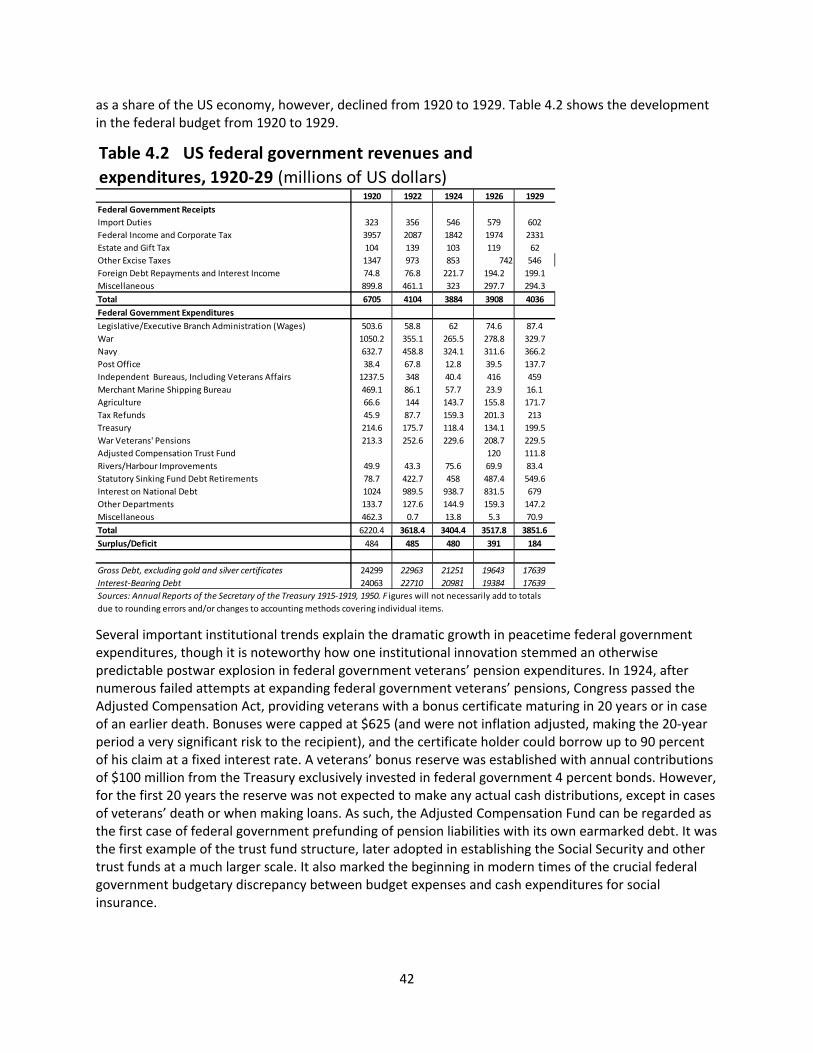
42  

as a share of the US economy, however, declined from 1920 to 1929. Table 4.2 shows the development in the federal budget from 1920 to 1929. 

 

Several important institutional trends explain the dramatic growth in peacetime federal government expenditures, though it is noteworthy how one institutional innovation stemmed an otherwise predictable postwar explosion in federal government veterans’ pension expenditures. In 1924, after numerous failed attempts at expanding federal government veterans’ pensions, Congress passed the Adjusted Compensation Act, providing veterans with a bonus certificate maturing in 20 years or in case of an earlier death. Bonuses were capped at $625 (and were not inflation adjusted, making the 20‐year period a very significant risk to the recipient), and the certificate holder could borrow up to 90 percent of his claim at a fixed interest rate. A veterans’ bonus reserve was established with annual contributions of $100 million from the Treasury exclusively invested in federal government 4 percent bonds. However, for the first 20 years the reserve was not expected to make any actual cash distributions, except in cases of veterans’ death or when making loans. As such, the Adjusted Compensation Fund can be regarded as the first case of federal government prefunding of pension liabilities with its own earmarked debt. It was the first example of the trust fund structure, later adopted in establishing the Social Security and other trust funds at a much larger scale. It also marked the beginning in modern times of the crucial federal government budgetary discrepancy between budget expenses and cash expenditures for social insurance. 

1920 1922 1924 1926 1929

Federal Government Receipts

Import Duties 323 356 546 579 602

Federal Income and Corporate Tax 3957 2087 1842 1974 2331

Estate and Gift Tax 104 139 103 119 62

Other Excise Taxes 1347 973 853 742 546

Foreign Debt Repayments and Interest Income 74.8 76.8 221.7 194.2 199.1

Miscellaneous 899.8 461.1 323 297.7 294.3

Total  6705 4104 3884 3908 4036

Federal Government Expenditures

Legislative/Executive Branch Administration (Wages) 503.6 58.8 62 74.6 87.4

War  1050.2 355.1 265.5 278.8 329.7

Navy 632.7 458.8 324.1 311.6 366.2

Post Office 38.4 67.8 12.8 39.5 137.7

Independent  Bureaus, Including Veterans Affairs 1237.5 348 40.4 416 459

Merchant Marine Shipping Bureau 469.1 86.1 57.7 23.9 16.1

Agriculture 66.6 144 143.7 155.8 171.7

Tax Refunds 45.9 87.7 159.3 201.3 213

Treasury 214.6 175.7 118.4 134.1 199.5

War Veterans' Pensions 213.3 252.6 229.6 208.7 229.5

Adjusted Compensation Trust Fund 120 111.8

Rivers/Harbour Improvements 49.9 43.3 75.6 69.9 83.4

Statutory Sinking Fund Debt Retirements 78.7 422.7 458 487.4 549.6

Interest on National Debt 1024 989.5 938.7 831.5 679

Other Departments 133.7 127.6 144.9 159.3 147.2

Miscellaneous 462.3 0.7 13.8 5.3 70.9

Total  6220.4 3618.4 3404.4 3517.8 3851.6

Surplus/Deficit 484 485 480 391 184

Gross Debt, excluding gold and silver certificates 24299 22963 21251 19643 17639

Interest‐Bearing Debt 24063 22710 20981 19384 17639

Table 4.2   US federal government revenues and 

expenditures, 1920‐29 (millions of US dollars)

Sources: Annual Reports of the Secretary of the Treasury 1915‐1919, 1950. F igures will not necessarily add to totals 

due to rounding errors and/or changes to accounting methods covering individual items.

43  

The 1920s saw the first examples of the federal government, through the Department of Commerce, engaging in industrial policy and directly attempting to subsidize selected American industries, such as commercial aeronautics and most profligately, under the political cover of national defense requirements, the US Merchant Marine. This type of federal financial support to key industries continues today through federal government defense contracts and in the case of the Merchant Marine, outright protectionism in the form of the Jones Act’s requirements that all goods transported by water between US ports be carried on US‐flagged vessels, built and owned in the United States and staffed by US citizens or green card holders. 

The federal government also greatly expanded its direct involvement in domestic infrastructure construction, and an attempt was even made in 1924 to explicitly use federal government infrastructure construction as a countercyclical stabilizer for the national economy. In 1928, Congress went further and considered, but ultimately rejected, the establishment of a “prosperity reserve” (e.g., earmarked prefunded trust fund), accessible only for funding public infrastructure during economic slowdowns. Had this proposal passed, it would have been a very early example—also for today’s European policymakers—of a potential high fiscal multiplier prefunded countercyclical federal government budget buffer. If such a prefunded “prosperity reserve” existed, it would also have been possible to consider in advance appropriate “shovel ready projects” available for rapid public investments in the next downturn. 

Probably the most important long‐term driver of federal government budget growth in the 1920s was the continued acceleration of grants‐in‐aid financial support to the US states by numerous federal government departments. In addition to supporting agriculture, the federal government began using this funding vehicle to support such diverse causes as states’ highway construction, vocational education, maternal/child healthcare, forest‐fire prevention, and prevention and treatment of sexually transmitted diseases. This expansion of grants‐in‐aid was driven by demands from the public (and an increasing number of Washington‐based national interest groups) that the federal government support many otherwise constitutionally designated “state and local functions,” as these often invariably overlapped with national concerns and interests. And not least by the realization that the federal government by now possessed a superior revenue‐raising ability to state and local governments. 

The requirement that states match federal grants‐in‐aid, and especially comply with various fixed standards set by federal law to be eligible for aid, proved a very powerful centralizing force. It clearly improved human and business conditions in many parts of the country and economy. But it also subjected states to the full fiscal powers of the federal government and to an increasingly permanent and intrusive federal government apparatus of administrative supervision and control. As such, the accelerating fiscal dominance and budgetary power achieved by the federal government during wartime manifested itself also as a more permanent peacetime integrating dynamism. 

 The federal government ran a fairly restrictive fiscal policy during the 1920s, though revenue collection was greatly aided in the short term by the economic boom and later in the decade increasingly by speculative boom. The greatest debate arose between those who favored rapid debt retirement and those pushing for lower taxes. In the end, a compromise emerged whereby the outstanding debt was reduced from about $25 billion to just under $17 billion (see table 4.2, and recall that as a share of GDP the decline was larger) and federal income taxes reduced significantly to a normal tax of only up to 5 percent and a marginal maximum surcharge tax of just 20 percent.  

Several relevant institutional features guided debt retirement efforts. First, Congress inserted in the last Liberty Bond issuance bill a statutory requirement that a sinking fund be established to retire the debt at a rate of an annual 2.5 percent cumulative of the outstanding debt on July 1, 1920 (roughly $20 billion), 

44  

minus foreign government obligations to the federal government on that date (almost $10 billion). In other words, the federal government sinking fund operated with an admittedly primitive “net government debt” concept when calculating annual budgetary allocations towards debt retirement. That such comprehensive thinking about what the meaningful measure of outstanding government debt means was present in the United States as early as 1920 is almost surprising, especially in light of the fixation on governments’ gross debt levels in the much more recent EU Treaties. 

Ultimately, this early government net debt concept proved dangerous, as many of America’s foreign claims were never repaid. Hence, the federal government debt was larger than earlier assumed and the annual relatively stable sinking fund cash allocation from the budget (about $500 million) was a smaller share of the total outstanding debt than initially intended. Of course, recalling how the EU Maastricht Treaty right from the beginning allowed for the fudging of the 60 percent debt/GDP requirement to enter into the euro, these early US difficulties in making government debt limits and reductions stick can be no surprise.  

Several Liberty Bond issues were also acceptable at par for paying federal government estate taxes, meaning that whenever such bonds fell below par, estate tax payers found it advantageous to purchase them for tax payment purposes, achieving an originally intended supportive function for the Liberty Bond market. And lastly, some of the special taxes implemented during the war, such as the franchise tax on the Federal Reserve System, were to politically facilitate their enactment earmarked towards debt retirement. 

US monetary policy making during the 1920s remained in its infancy and was subsumed under the general easy money policies of the US Treasury. Open market operations—e.g., direct buying and selling of federal government bonds for credit stabilization purposes—were initiated in 1923. Most importantly, the new Federal Reserve System during the 1920s failed to materially reduce the high number of bank failures in the US economy, partly due to the weakening of capital requirements implemented during the war. Total bank failures from 1920 to 1929, generally a period of high economic growth, were a staggering 5,712, of which almost a thousand were nationally chartered or state members of the Federal Reserve System. Total losses to depositors during the 1920s were in excess of half a billion dollars.  

Lastly, when considering institutional developments during the 1920s, it is important to recognize that while World War I was a huge boost to the federal government, longer and more pervasive economic and political forces drove an even larger growth for state and local governments in the United States. From 1900 to 1929, federal government expenditures rose approximately six times, but local government expenditures rose seven times and state governments no less than 15 times during the same period. Hence by the earliest comparable data from 1932, total state and local government expenses were at a combined over $9.2 billion almost twice the magnitude of total federal government expenses (which had risen rapidly after 1929). Two factors mostly drove this rapid growth: growth of automobile ownership and associated need for new road construction and the large expansion of primary and secondary education during the first decades of the 20th century. Both areas were almost exclusively the responsibility of state and local government, though in time were increasingly supported by federal government grants‐in‐aid. 

State and local government revenue collection was dominated by volatile property and motor vehicle registration taxes, with only a much smaller share coming from income taxation. At the same time, indebtedness of particular local governments—not bound by states’ constitutional debt limitations—rose rapidly for infrastructure investments. As a result, state and local government gross debts had risen 

45  

to a total of $19.6 billion by 1932,35 or approximately the same as the level of federal government debt that year. General US government debts at the time were hence basically evenly split between federal and state and local government levels. 

In some ways, it might be argued that the early 20th century and especially the 1920s marked a period of actual government decentralization in the US economy, based on the faster growth of state and local government budgets. This, however, is a wrong characterization for at least two reasons: first the federal government increasingly supported state and local governments through grants‐in‐aid, and second fiscal sustainability of the federal government (surplus) and state and local governments (rising deficits) was vastly different at the end of the 1920s. The growth of state and local government activities was, therefore, and especially in light of the federal government’s stronger potential fiscal powers, built on a very shaky foundation that the Great Depression would severely erode. 

4.3 US Institutional Innovations during the Great Depression and the New Deal(s) 

The collapse of the American economy between 1929 and 1933 and the slow and repeatedly disrupted recovery in the years until the United States joined World War II in 1941 amounted to a political emergency that was in many ways the functional equivalent of earlier periods of war. From the perspective of the scope of federal government institutions and congressional willingness to develop and use them, this period was another one of rapid growth. During the 1930s the federal government began providing generally available social assistance to large groups of the American people and became completely fiscally dominant in its relations with state and local governments. Indeed, many of the governing institutions that still shape the federal budget and the lives of most Americans were established during this period. 

The federal government reacted slowly to the Great Depression, as President Hoover and congressional leaders only gradually grasped the depth of the crisis. Initially therefore the policy response was mostly to use existing government institutions more intensively to try to restore economic growth and end deflation. Only once Franklin D. Roosevelt was elected president in 1933—four years into the economic collapse—were entirely new and often quite revolutionary new federal government institutions and policies proposed and implemented. 

Despite his administration’s public pursuit of federal government fiscal rectitude and balanced budgets, President Hoover greatly expanded the federal government’s public infrastructure investments with the explicit aim of boosting employment. This included a huge building bonanza of federal government buildings still dominating central Washington, DC today, hundreds of millions of dollars more for river and harbor improvements and the Colorado River dam (often called the Hoover Dam). Congress passed the Emergency Construction Appropriations Act and Emergency Relief and Construction Act in 1930 and 1932, respectively, which greatly increased the federal government grants‐in‐aid to states for highway construction. The latter Act, though, went much farther and provided federal government grants to states to be used towards any public infrastructure investment and crucially to provide—via states—direct financial relief to individual Americans. In other words, in 1932, the federal government indirectly began financing direct social benefits to individuals. The Emergency Relief and Construction Act also established the Reconstruction Finance Corporation (RFC), a wholly federally owned financial entity, 

                                                            35 US state governments accounted for $2.9 billion and various local government entities, noticeably larger cities, accounted for the bulk at $16.7 billion. That state governments, despite earlier constitutional debt restrictions, amassed almost $3 billion in debt shows that economic booms can also sway the fiscal conservatism of electorates. Numerous states had passed specific bond issuances earmarked for various infrastructure, veterans’ bonuses, or social policy purposes in public referenda overriding state constitutional limitations. 

46  

tasked with lending money to state governments unable to afford extend social assistance and other benefits to state residents, as well as providing financing to private entities like banks, firms, and farmers unable to access it elsewhere.  

Money lent by the RFC to state governments was initially supposed to be repaid after three years and carried—during a deeply deflationary period—a high interest of 3 percent annually. As such, RFC loans in some ways mirrored federal government loans made to states during the economic crisis of 1837, though at that time federal government surpluses were being distributed as interest‐free loans never to be repaid. Two years later, in 1934 Congress, recognizing the still deep economic crisis and implausibility of repayment ever, converted the RFC loans to state governments into gifts. The political, financial, and economic circumstances surrounding these Great Depression RFC loans (and the interest‐free “loans” of 1837) and today’s ESM loans to Greece are surprisingly similar. Both started out as crisis loans made by the central fiscal authority to suffering state/member state governments at relatively high interest rates and short maturity but as the economic circumstances deteriorated were gradually converted into more and more concessional loans. In the case of the United States, the conversion from loan to gift (e.g., 100 percent debt relief) took just two years, whereas in the less politically integrated euro area, the process has been more drawn out and conditional and may not ultimately see the full loan value completely forgiven, though Greece will in the end repay the ESM far less than the full net present value of the loans granted. 

RFC loan provisions to private entities meanwhile were excessively rigorous and had a problematic focus on credit risk prevention. Loans could be made only against “full and adequate security” (e.g., top‐quality collateral), which made it impossible for many of the most financially struggling businesses to access them, greatly reducing the ability of the RFC to assist in the economic recovery. The Act moreover contained a highly damaging provision requiring the names of borrowers and the terms of the loan to be made public. Given that numerous banks applied for RFC loans, the publication of often highly sensitive financial information about a bank in financial problems often added to the risk of a run against it. This aggravated banking sector fragility in late 1932, as Franklin D. Roosevelt was getting ready to take over as president. A particular loan made by the RFC was to set up the federal government’s new Home Loan Bank, which was to provide direct financial aid to homeowners by offering to repurchase (or rediscount) the first mortgages from lending institutions. Due to limitations on the size and maturities of mortgages repurchased, the Home Loan Bank program did not, however, provide material financial aid to US homeowners and mostly inspired the much larger institutions created by the subsequent Roosevelt administration. 

An important change was made to the Federal Reserve Act in 1932 in response to the economic crisis and the ensuing rapid decline in outstanding commercial paper. The dearth of commercial paper made it more difficult for the Federal Reserve banks, which could back up to 60 percent of their issued bank notes with commercial paper rather than gold, to continue the intended antideflationary expansion of the US money supply. As part of the Glass‐Steagall Act of 1932, the Federal Reserve banks were allowed to use federal government debt, rather than commercial paper, as collateral for their issued paper money, further cementing the economic and financial relations between the US federal government and its central bank. Crucially, this change enabled the Federal Reserve banks to purchase potentially very large quantities of federal government debt without risking contracting the outstanding US money supply in the process and hence facilitated the more ambitious open market operations initiated by the Federal Reserve in the spring of 1932 to stimulate activity and credit to the real economy. Federal Reserve holdings of federal government debt rose from $840 million in March 1932 to $1.8 billion by July, though these purchases, in the face of the still accelerating depression, ultimately failed at their stimulative intent. 

47  

Towards the end of his term, President Hoover in a futile attempt to balance the federal government budget appealed to Congress to increase tax revenues by reversing many of the tax reductions implemented after World War I. Congress approved and in the midst of the depression in June 1932 passed the (still today) largest peacetime tax increase in US history. Income tax exemptions were slashed, normal taxes doubled and surcharge taxes were raised up to a maximum of 55 percent, while estate, corporate, and excise taxes were also significantly increased. The fiscal response was unsurprising, though it must be noted that Keynesian economics was not yet accepted by mainstream policymakers in the United States or elsewhere, as actually collected revenues dropped and the depression deepened from the reduction in economic activity arising from the increased tax burden. 

As the economic crisis deepened during 1932, the US banking system deteriorated dramatically and several US states were forced to declare lengthy banking holidays. The declaration of a statewide indefinite banking holiday in Michigan on February 14, 1932 led to widespread contagion to other US states. Other states were quickly forced into taking similar measures, as bank customers across the country, fearful of future bank failures and/or loss of access to their deposits, hoarded cash.36 As a result, the majority of US states had already declared statewide banking holidays, or otherwise restricted access to bank deposits when the newly inaugurated President Roosevelt declared a national US banking holiday on March 5, 1933. Roosevelt’s declaration, however, crucially created a uniform national policy response to the banking crisis and forcefully transferred the political and financial responsibility for its resolution to the federal government, which unlike the states had the fiscal resources to do so. Acute crisis once again caused a dramatic centralization move and transferred responsibilities to the federal government untouchable in normal political times. 

During the banking holiday, Congress passed the Emergency Banking Act of 1933, which greatly expanded federal government (e.g., presidential) authority over banking regulation and precious metal exchange, including a compulsory federal government evaluation of individual bank solvency before they could reopen. The RFC was enabled to—if required—inject federal government money as preferred stock in solvent, but undercapitalized, banks. Lastly, the Federal Reserve System was empowered to issue emergency currency backed by any asset of a solvent commercial bank. 

Combined with Roosevelt’s forceful public interventions to stem the financial panic—the so‐called presidential fireside chats transmitted on radio—the national banking holiday and Emergency Banking Act are widely credited by contemporary commentators as having been the turning point in the Great Depression. The Act contained all the important elements of an effective government response to a systemic banking crisis: It introduced in the RFC a government fiscal backstop for the US banking system, issued an (at least implicit) initial 100 percent deposit guarantee covering all solvent and reopened US banks, and with a federal government financial guarantee enabled the Federal Reserve banks to be true lenders of last resort and lend without restrictions to liquidity‐challenged banks. The lasting importance of the Emergency Act is its continuing empowerment of the federal government in banking supervision and regulation and the ability it gave President Roosevelt to voluntarily take the United States off the gold standard. It also was the precursor of the introduction of permanent retail deposit insurance in the United States with the Banking Act of 1933 signed by President Roosevelt in June that year. The establishment of the Federal Deposit Insurance Corporation (FDIC) arguably marked the greatest centralizing move in the American banking sector to date. The FDIC, as a single insurance provider for the American public, is considerably more centralized than the banking supervision, regulation, or 

                                                            36 Currency in circulation in large denominations of $50 or higher rose by about 30 percent from February 15 to the national banking holiday declared on March 5 (Federal Reserve Board 1933, 5). Many depositors, moreover, fearful of future devaluations increasingly sought to convert their savings into gold. 

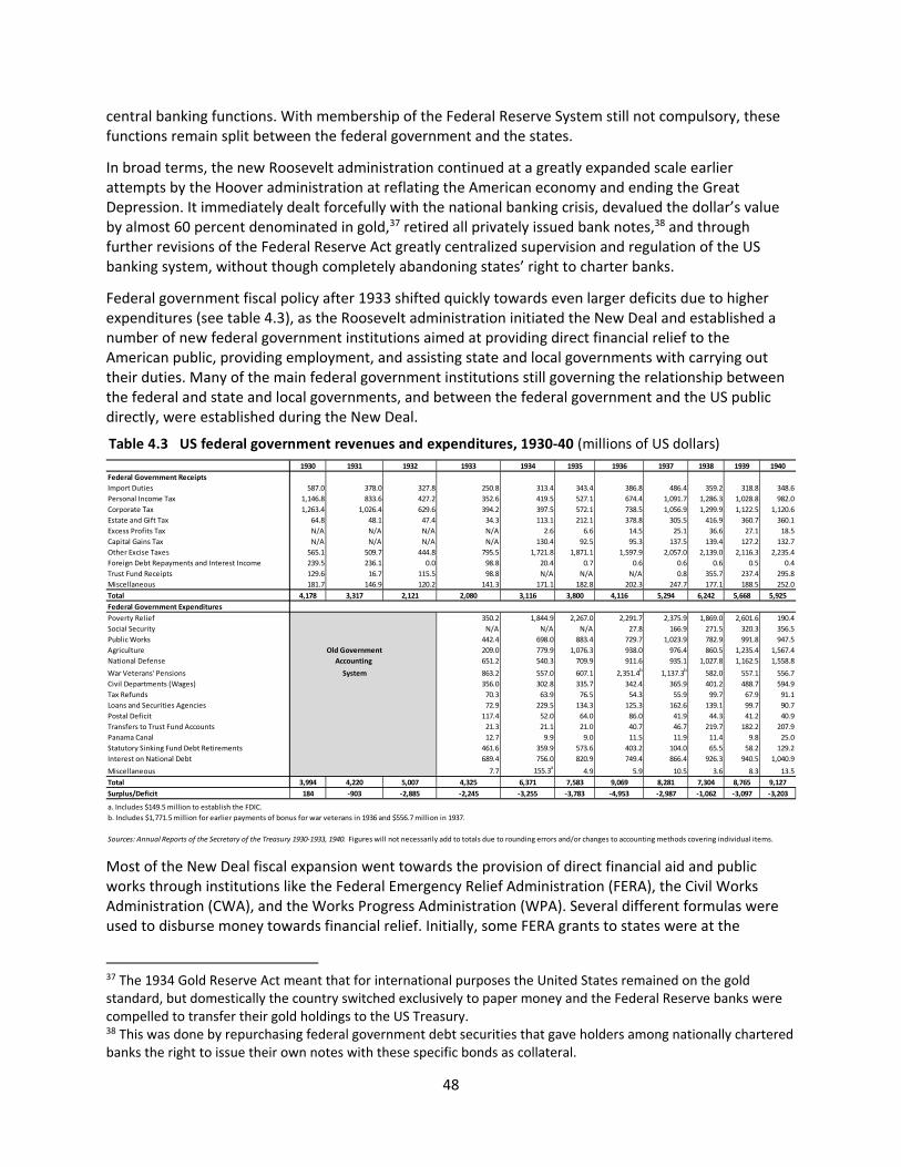
48  

central banking functions. With membership of the Federal Reserve System still not compulsory, these functions remain split between the federal government and the states. 

In broad terms, the new Roosevelt administration continued at a greatly expanded scale earlier attempts by the Hoover administration at reflating the American economy and ending the Great Depression. It immediately dealt forcefully with the national banking crisis, devalued the dollar’s value by almost 60 percent denominated in gold,37 retired all privately issued bank notes,38 and through further revisions of the Federal Reserve Act greatly centralized supervision and regulation of the US banking system, without though completely abandoning states’ right to charter banks.  

Federal government fiscal policy after 1933 shifted quickly towards even larger deficits due to higher expenditures (see table 4.3), as the Roosevelt administration initiated the New Deal and established a number of new federal government institutions aimed at providing direct financial relief to the American public, providing employment, and assisting state and local governments with carrying out their duties. Many of the main federal government institutions still governing the relationship between the federal and state and local governments, and between the federal government and the US public directly, were established during the New Deal. 

 

Most of the New Deal fiscal expansion went towards the provision of direct financial aid and public works through institutions like the Federal Emergency Relief Administration (FERA), the Civil Works Administration (CWA), and the Works Progress Administration (WPA). Several different formulas were used to disburse money towards financial relief. Initially, some FERA grants to states were at the 

                                                            37 The 1934 Gold Reserve Act meant that for international purposes the United States remained on the gold standard, but domestically the country switched exclusively to paper money and the Federal Reserve banks were compelled to transfer their gold holdings to the US Treasury. 38 This was done by repurchasing federal government debt securities that gave holders among nationally chartered banks the right to issue their own notes with these specific bonds as collateral. 

1930 1931 1932 1933 1934 1935 1936 1937 1938 1939 1940

Federal Government Receipts

Import Duties 587.0 378.0 327.8 250.8 313.4 343.4 386.8 486.4 359.2 318.8 348.6

Personal Income Tax 1,146.8 833.6 427.2 352.6 419.5 527.1 674.4 1,091.7 1,286.3 1,028.8 982.0

Corporate Tax 1,263.4 1,026.4 629.6 394.2 397.5 572.1 738.5 1,056.9 1,299.9 1,122.5 1,120.6

Estate and Gift Tax 64.8 48.1 47.4 34.3 113.1 212.1 378.8 305.5 416.9 360.7 360.1

Excess Profits Tax N/A N/A N/A N/A 2.6 6.6 14.5 25.1 36.6 27.1 18.5

Capital Gains Tax N/A N/A N/A N/A 130.4 92.5 95.3 137.5 139.4 127.2 132.7

Other Excise Taxes 565.1 509.7 444.8 795.5 1,721.8 1,871.1 1,597.9 2,057.0 2,139.0 2,116.3 2,235.4

Foreign Debt Repayments and Interest Income 239.5 236.1 0.0 98.8 20.4 0.7 0.6 0.6 0.6 0.5 0.4

Trust Fund Receipts 129.6 16.7 115.5 98.8 N/A N/A N/A 0.8 355.7 237.4 295.8

Miscellaneous 181.7 146.9 120.2 141.3 171.1 182.8 202.3 247.7 177.1 188.5 252.0

Total  4,178 3,317 2,121 2,080 3,116 3,800 4,116 5,294 6,242 5,668 5,925

Federal Government Expenditures

Poverty Relief 350.2 1,844.9 2,267.0 2,291.7 2,375.9 1,869.0 2,601.6 190.4

Social Security N/A N/A N/A 27.8 166.9 271.5 320.3 356.5

Public Works 442.4 698.0 883.4 729.7 1,023.9 782.9 991.8 947.5

Agriculture Old Government 209.0 779.9 1,076.3 938.0 976.4 860.5 1,235.4 1,567.4

National Defense Accounting  651.2 540.3 709.9 911.6 935.1 1,027.8 1,162.5 1,558.8

War Veterans' Pensions System 863.2 557.0 607.1 2,351.4b

1,137.3b

582.0 557.1 556.7

Civil Departments (Wages) 356.0 302.8 335.7 342.4 365.9 401.2 488.7 594.9

Tax Refunds 70.3 63.9 76.5 54.3 55.9 99.7 67.9 91.1

Loans and Securities Agencies 72.9 229.5 134.3 125.3 162.6 139.1 99.7 90.7

Postal Deficit 117.4 52.0 64.0 86.0 41.9 44.3 41.2 40.9

Transfers to Trust Fund Accounts 21.3 21.1 21.0 40.7 46.7 219.7 182.2 207.9

Panama Canal 12.7 9.9 9.0 11.5 11.9 11.4 9.8 25.0

Statutory Sinking Fund Debt Retirements 461.6 359.9 573.6 403.2 104.0 65.5 58.2 129.2

Interest on National Debt 689.4 756.0 820.9 749.4 866.4 926.3 940.5 1,040.9

Miscellaneous 7.7 155.3a

4.9 5.9 10.5 3.6 8.3 13.5

Total  3,994 4,220 5,007 4,325 6,371 7,583 9,069 8,281 7,304 8,765 9,127

Surplus/Deficit 184 ‐903 ‐2,885 ‐2,245 ‐3,255 ‐3,783 ‐4,953 ‐2,987 ‐1,062 ‐3,097 ‐3,203

a. Includes $149.5 million to establish the FDIC.

b. Includes $1,771.5 million for earlier payments of bonus for war veterans in 1936 and $556.7 million in 1937.

Sources: Annual Reports of the Secretary of the Treasury 1930‐1933, 1940. Figures will not necessarily add to totals due to rounding errors and/or changes to accounting methods covering individual items.

Table 4.3   US federal government revenues and expenditures, 1930‐40 (millions of US dollars)

49  

discretion of the federal government itself, whereas others could initially be commanded by the states if they committed their own (larger share of) funding as well. As the Depression continued and states’ fiscal situation deteriorated, however, all funds were disbursed by the federal government itself and without the need for any matching state and local funds. As a result in the early 1930s the federal government became the dominant fiscal guarantor for financial assistance given directly to the American public. This, however, was a controversial policy, as traditionally direct financial relief to individuals had been viewed as solely a state and especially local government matter. Roosevelt himself saw federal government involvement as solely a temporary crisis phenomenon and preferred to act through federal employment creation initiatives. As he stated in his 1935 Annual Message to Congress: 

More than two billions of dollars have also been expended in direct relief to the destitute. Local agencies of necessity determined the recipients of this form of relief. With inevitable exceptions the funds were spent by them with reasonable efficiency and as a result actual want of food and clothing in the great majority of cases has been overcome. 

But the stark fact before us is that great numbers still remain unemployed. 

A large proportion of these unemployed and their dependents have been forced on the relief rolls. The burden on the Federal Government has grown with great rapidity. We have here a human as well as an economic problem. When humane considerations are concerned, Americans give them precedence. The lessons of history, confirmed by the evidence immediately before me, show conclusively that continued dependence upon relief induces a spiritual and moral disintegration fundamentally destructive to the national fibre. To dole out relief in this way is to administer a narcotic, a subtle destroyer of the human spirit. It is inimical to the dictates of sound policy. It is in violation of the traditions of America. Work must be found for able‐bodied but destitute workers. 

The Federal Government must and shall quit this business of relief. 

I am not willing that the vitality of our people be further sapped by the giving of cash, of market baskets, of a few hours of weekly work cutting grass, raking leaves or picking up papers in the public parks. We must preserve not only the bodies of the unemployed from destitution but also their self‐respect, their self‐reliance and courage and determination. This decision brings me to the problem of what the Government should do with approximately five million unemployed now on the relief rolls. 

About one million and a half of these belong to the group which in the past was dependent upon local welfare efforts. Most of them are unable for one reason or another to maintain themselves independently—for the most part, through no fault of their own. Such people, in the days before the great depression, were cared for by local efforts—by States, by counties, by towns, by cities, by churches and by private welfare agencies. It is my thought that in the future they must be cared for as they were before. I stand ready through my own personal efforts, and through the public influence of the office that I hold, to help these local agencies to get the means necessary to assume this burden. 

The security legislation which I shall propose to the Congress will, I am confident, be of assistance to local effort in the care of this type of cases. Local responsibility can and will be 

50  

resumed, for, after all, common sense tells us that the wealth necessary for this task existed and still exists in the local community, and the dictates of sound administration require that this responsibility be in the first instance a local one. There are, however, an additional three and one half million employable people who are on relief. With them the problem is different and the responsibility is different. This group was the victim of a nation‐wide depression caused by conditions which were not local but national. The Federal Government is the only governmental agency with sufficient power and credit to meet this situation. We have assumed this task and we shall not shrink from it in the future. It is a duty dictated by every intelligent consideration of national policy to ask you to make it possible for the United States to give employment to all of these three and one half million employable people now on relief, pending their absorption in a rising tide of private employment. 

Federal government public infrastructure investment also rose dramatically to almost $1 billion annually by the end of the 1930s, with the majority of funds going towards highway construction and national park infrastructure. The Public Works Administration (PWA), which oversaw the expansion of federal infrastructure investments, could also support state infrastructure projects with up to 30 percent grant funding and the remaining 70 percent covered through a loan. To a very large extent, the federal government stepped in as the “infrastructure investor of last resort” and took over, as state and local governments and private investors rapidly reduced their outlays in this category. 

The New Deal also saw important innovations in other social policy areas. Most importantly, in 1935 Congress passed the Social Security Act, establishing generally available old age pensions in the United States; facilitated states’ unemployment insurance schemes; and provided states with grant funding for old age assistance, public health, aid to the blind and handicapped, and other social causes, as well as for the administration of states’ unemployment schemes. 

Federal government old age pensions, or Social Security, again utilized the trust fund model and earmarked payroll tax revenue towards the provision of old age pensions on a modified pay‐as‐you‐go‐basis. Contributions from employers and employees went into a separate trust fund, exclusively invested in federal government debt, paying out benefits as recipient became eligible upon turning 65.39 

The new unemployment insurance scheme was more complicated, as it instituted a new federal payroll tax by 1937 of 3 percent at companies with eight employees or more. Provided, however, that states implemented a state unemployment insurance scheme that adhered to federal guidelines, employers could offset up to 90 percent of the federal government payroll tax by making payments into their state unemployment insurance scheme. Or in other words, the federal government kept only 0.3 percentage points of the new payroll tax, funds from which it gave states grants to administer their new unemployment insurance schemes.40 All proceeds from states’ own schemes, however, had to be paid into a central unemployment trust fund in the US Treasury, from which states could then withdraw money as required to pay benefits to their unemployed. 

This institutional setup first greatly incentivized all states to set up their own unemployment insurance schemes, as the revenues from the 3 percent federal payroll tax would otherwise be lost to their unemployed. It also provided the states with the freedom to establish their own unemployment 

                                                            39 US average life expectancy in 1935 was just 59.9 years for men and 63.9 for women respectively. However, since this was due to the still high infant mortality in the United States at the time, it is important to realize that if Americans in 1935 made it to working age and began contributing to the Social Security system, they had a good chance of also turning 65 and enjoying Social Security benefits for a substantial period in retirement afterwards. 40 Only a few states had their own unemployment schemes prior to 1935. 

51  

insurance schemes with the benefit and contribution levels at or above the federally mandated level. As a result, even today, the provision of unemployment benefits in the United States varies greatly among the states, and the federal government usually gets financially involved only in cases of national recessions (see part II below for a detailed description of the system today). 

In 1936, Congress further approved a change to the World War I veterans’ trust fund, enabling veterans to take out their bonuses immediately. Many did, and this measure provided a sizable short‐term fiscal stimulus in 1936‐37, proving that with sufficient political will even the trust fund structure can relatively easily be tweaked to provide such short‐term stimulus.  

The Roosevelt administration also initiated a series of initiatives to provide relief directly to struggling homeowners. The new Home Owners Loan Corporation took over distressed mortgages directly, the Federal Housing Administration offered insurance for most smaller mortgages, and from 1938 the Federal National Mortgage Association (Fannie Mae) was tasked with creating a secondary mortgage market by securitizing Americans’ mortgages into mortgage‐backed securities. The extraordinary degree of present‐day federal government intervention in the US housing market hence began as part of Roosevelt’s New Deal. The same is true for the abiding federal government financial support to the US agricultural sector. During the New Deal the federal government began subsidized lending, paid subsidies to reduce production (e.g., raise prices), provided aid to tenant farmers without their own land, facilitated farm modernizations, and expanded the general educational and regulatory activities of the US Department of Agriculture.  

Several elements of the New Deal programs, most noticeably the Social Security old‐age pension program, greatly increased the federal government’s use of the trust fund financing model for the provision of federal government social benefits. Prior to the New Deal, the trust fund model was used only for the provision of World War I veterans’ pensions, and its share—$323 million—of total federal government interest‐bearing debt was very small at only approximately 1.5 percent. By 1940, however, the size of federal government trust funds earmarked for social benefit provision had increased dramatically to $4.8 billion, or 11.5 percent of total interest‐bearing debt. As will be discussed further in Part II below, today such intragovernment holdings of trust fund debt, which marks the difference between the concept of federal government “debt held by the public” and total federal government debt outstanding, have increased further and at the end of 2016 amounted to $5.5 trillion, or approximately 27.6 percent of total federal government debt. 

The popularity of the trust fund model for social benefit provision by the federal government is not hard to understand. By essentially earmarking significant amounts of future federal government taxation and borrowing towards a specific predetermined purpose, it likely facilitated the political acceptance of the federal government taking on such identified (and sizable) budgetary tasks. The sizable earmarked payroll taxes that flow into the trust funds and here creates a financial benefit (or entitlement) in the name of each participating individual would likely have faced considerably more political resistance if they had merely flowed into the regular federal government budget and could be allocated according to the annual whims of Congress. The federal government trust fund model of earmarked taxation has likely facilitated a higher degree of fiscal policy and institutional centralization in the United States than would have been politically possible without it. The political palpability and public acceptance of the type of earmarked taxes represented by federal government trust funds should be of obvious interest to today’s EU policymakers (this issue will be elaborated below in Part II). 

The great expansion of the US federal government associated with the New Deal quite naturally relegated US state and local government to a historically new fiscally dependent position. State and local governments became permanently and increasingly dependent on federal government grants and 

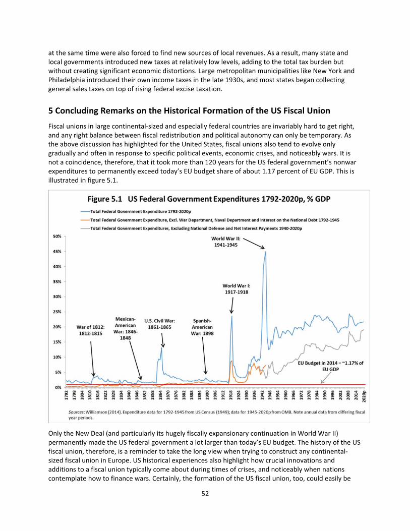
52  

at the same time were also forced to find new sources of local revenues. As a result, many state and local governments introduced new taxes at relatively low levels, adding to the total tax burden but without creating significant economic distortions. Large metropolitan municipalities like New York and Philadelphia introduced their own income taxes in the late 1930s, and most states began collecting general sales taxes on top of rising federal excise taxation.  

 5 Concluding Remarks on the Historical Formation of the US Fiscal Union 

Fiscal unions in large continental‐sized and especially federal countries are invariably hard to get right, and any right balance between fiscal redistribution and political autonomy can only be temporary. As the above discussion has highlighted for the United States, fiscal unions also tend to evolve only gradually and often in response to specific political events, economic crises, and noticeably wars. It is not a coincidence, therefore, that it took more than 120 years for the US federal government’s nonwar expenditures to permanently exceed today’s EU budget share of about 1.17 percent of EU GDP. This is illustrated in figure 5.1. 

 

Only the New Deal (and particularly its hugely fiscally expansionary continuation in World War II) permanently made the US federal government a lot larger than today’s EU budget. The history of the US fiscal union, therefore, is a reminder to take the long view when trying to construct any continental‐sized fiscal union in Europe. US historical experiences also highlight how crucial innovations and additions to a fiscal union typically come about during times of crises, and noticeably when nations contemplate how to finance wars. Certainly, the formation of the US fiscal union, too, could easily be 

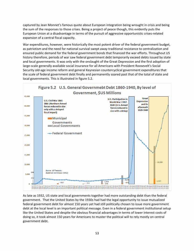
53  

captured by Jean Monnet’s famous quote about European integration being wrought in crisis and being the sum of the responses to those crises. Being a project of peace though, this evidently puts the European Union at a disadvantage in terms of the pursuit of aggressive opportunistic crises‐related expansion of a central fiscal capacity.  

War expenditures, however, were historically the most potent driver of the federal government budget, as patriotism and the need for national survival swept away traditional resistance to centralization and ensured public demand for the federal government bonds that financed the war efforts. Throughout US history therefore, periods of war saw federal government debt temporarily exceed debts issued by state and local governments. It was only with the onslaught of the Great Depression and the first adoption of large‐scale generally available social insurance for all Americans with President Roosevelt’s Social Security old‐age income reform and general Keynesian countercyclical government expenditures that the scale of federal government debt finally and permanently soared past that of the total of state and local governments. This is illustrated in figure 5.2. 

 

As late as 1932, US state and local governments together had more outstanding debt than the federal government.  That the United States by the 1930s had had the legal opportunity to issue mutualized federal government debt for almost 150 years yet had still politically chosen to issue more government debt at the local level is an important political message. Even in a federal government institutional setup like the United States and despite the obvious financial advantages in terms of lower interest costs of doing so, it took almost 150 years for Americans to muster the political will to rely mostly on central government debt.  

54  

This puts into a perspective just how aggressive some proposals for the introduction of Eurobonds would be. Weizsäcker and Delpla (2011), for instance, suggest moving to 60 percent of GDP Blue (mutualized) bonds. With euro area general government gross debt of about 90 percent in 2017, this level would imply that two‐thirds of all governmental debt was mutualized. Per figure 5.2, only the dramatic costs to the federal government of fighting the Great Depression and preparing to fight World War II achieved such an outcome in the United States. 

Figure 5.2 also highlights the importance of municipal debt relative to state government debt throughout the early 20th century. This fact is an important illustration of how the US general government—even as the federal government in the early 20th century remained without regular income‐based revenue and state governments were bound by self‐imposed borrowing constraints— expanded infrastructure investments and social services at the often less constrained municipal level (especially in major metropolitan cities) during an era of rapid urbanization and overall population increase. A degree of “fiscal subsidiarity” can hence be said to have existed in the United States prior to the federal government assuming the dominant fiscal role, as local governments expanded their activities and services ahead of these same offerings (occasionally as with Social Security taken over by the federal government) being made available throughout the entire country. 

A comprehensive analysis of US fiscal history shows that fiscal unions emerge only slowly, in response to particular political events, and remain highly path dependent. Despite the self‐evident epochal differences between the United States and the EU/euro area, it is instructive to consider the respective timelines for the two in establishing the most important characteristics of an integrated fiscal union. Table 5.1 shows the elements of a fiscal union aiming to (1) achieve sound lower‐level government fiscal policies; (2) facilitate budgetary fiscal transfers between lower‐level government units; (3) provide credible common fiscal backstops in crises; and (4) enable common borrowing backed by joint guarantee/revenue and provision of a safe financial asset.41 

                                                            41 See IMF (2013) for an overview of the main components of a fiscal union. 

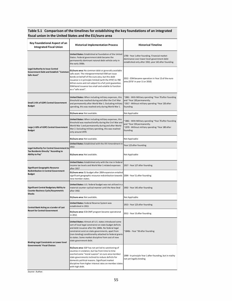
55  

 

Key Foundational Aspect of an 

Integrated Fiscal UnionHistorical Implementation Process Historical Timeline

United States: Established at foundation of the United 

States. Federal government debt became the 

permanently dominant naional debt vehicle only in 

the early 1930s.

1790 ‐ Year 1 after founding. Financial market 

dominance over lower level government debt 

established only after 1932, year 142 after founding

EU/euro area: No common debt or generally available 

safe asset. The intergovernmental ESM can issue 

bonds on behalf of the euro area, but this debt 

issuance is in principle limited (with the EFSF) to 700 

billion euros and not subject to a full joint guarantee. 

ESM bond issuance too small and volatile to function 

as a "safe asset".

2012 ‐ ESM became operation in Year 13 of the euro 

area (EFSF in year 11 or 2010)

United States: When including military expenses, this 

threshold was reached during and after the Civil War 

and permanently after World War 1. Excluding military 

spending, this was reached only during World War 1.

~1861 ‐ With Military spending ~Year 70 after founding 

and ~Year 130 permanently.                                                        

~1917 ‐ Without military spending ~Year 130 after 

founding

EU/euro area: Not available. Not Applicable

United States: When including military expenses, this 

threshold was reached briefly during the Civil War and 

World War 1 and permanently during and after World 

War 2. Excluding military spending, this was reached 

only around 1970.

~1861 ‐ With Military spending ~Year 70 after founding 

and ~Year 150 permanently.                                                        

~1970 ‐ Without military spending ~Year 180 after 

founding

EU/euro area: Not available. Not Applicable

United States: Established with the XIV Amendment in 

1913Year 123 after founding

EU/euro area: Not available. Not Applicable

United States: Established only with the rise in federal 

income tax levels and World War 1 related expenses 

after 1917

1917 ‐ Year 127 after founding

EU/euro area: EU budget after 2004 expansion entailed 

significant geographic resource redistribution towards 

new member states.

2004 ‐ Year 51 after founding

United States: U.S. federal budget was not utilized in a 

material counter‐cyclical manner until the New Deal 

after 1932.

1932 ‐ Year 142 after founding

EU/euro area: Not available. Not Applicable

United States: Federal Reserve System was 

established in 1913.1913 ‐ Year 123 after founding

EU/euro area: ECB OMT program became operational 

in 2012.2012 ‐ Year 13 after founding

United States: Almost all U.S. states introduced some 

sort of local legal constrainst on state budget deficits 

and debt issuance after the 1840s. No federal legal 

constrainst exist on state governments, apart from 

(non‐binding) conditionality attached to federal grants 

to states. Some market discipline from cost of new 

state government debt.

~1840s ‐ Year ~50 after founding

EU/euro area: SGP has not yet led to sanctioning of 

counties in violation, but has from time to time 

exerted some "moral suasion" on euro area member 

state governments inclined to reduce deficits for 

domestic political reasons. Significant market 

discipline from higher interest rates on member states 

with high debt.

1999 ‐ In principle Year 1 after founding, but in reality 

not yet legally binding

Source: Author.

Binding Legal Constraints on Lower level 

Governments' Fiscal Choices

Table 5.1   Comparison of the timelines for establishing the key foundations of an integrated 

fiscal union in the United States and the EU/euro area

Significant Central Budgetary Ability to 

Counter Business Cycle/Assymmetric 

Shocks

Legal Authority to Issue Central 

Government Debt and Establish "Common 

Safe Asset"

Large (>10% of GDP) Central Government 

Budget

Small (>5% of GDP) Central Government 

Budget

Legal Authority For Central Government to 

Tax Residents Directly "According to 

Ability to Pay"

Significant Geographic Resource 

Redistribution in Central Government 

Budget

Central Bank Acting as a Lender of Last 

Resort for Central Government

56  

 

Table 5.1 illustrates that the United States today has a complete fiscal union, while the EU/euro area lacks important components. These include control over significant direct government revenue (e.g., taxing powers), capacity to act as an economically material centralized budget able to implement countercyclical fiscal policies, and arguably binding constraints on lower level government fiscal policies. At the same time, table 5.1 highlights how the political process in the United States creating today’s institutions frequently took well over a century from the country’s founding.  Moreover, on issues such as the central bank’s ability to act as a lender of last resort and shifting significant budgetary resources between lower‐level government entities, the ECB and post‐2004 EU budget,42 compared with the United States, look demonstratively ahead of their time, having been implemented at a much earlier stage of existence. In other words, European fiscal integration in level terms remains far behind the United States but much less so when the time dimension is added. 

Another way to compare the current scope of the US and European fiscal unions is to compare which level of government controls which elements of standard revenue generation and core government expenditure functions. Given the self‐evident differences between the two entities, however, such comparisons are meaningful only in an aspirational sense to identify areas in which a future European level fiscal union could expand in scope. This is done in table 5.2.43 

                                                            42 Part II shows that some new EU member states currently receive up to 5 percent of GDP in annual transfers from the existing EU budget. Such a level of sustained resource transfers to individual member states (despite not amounting to a high share of overall EU GDP) must sensibly be classified as material fiscal transfers. These transfers, however, are not particularly relevant in addressing asymmetric shocks. 43 See Kirkegaard (2015a) for an in‐depth analysis of the division of tasks between governmental levels in the United States. 

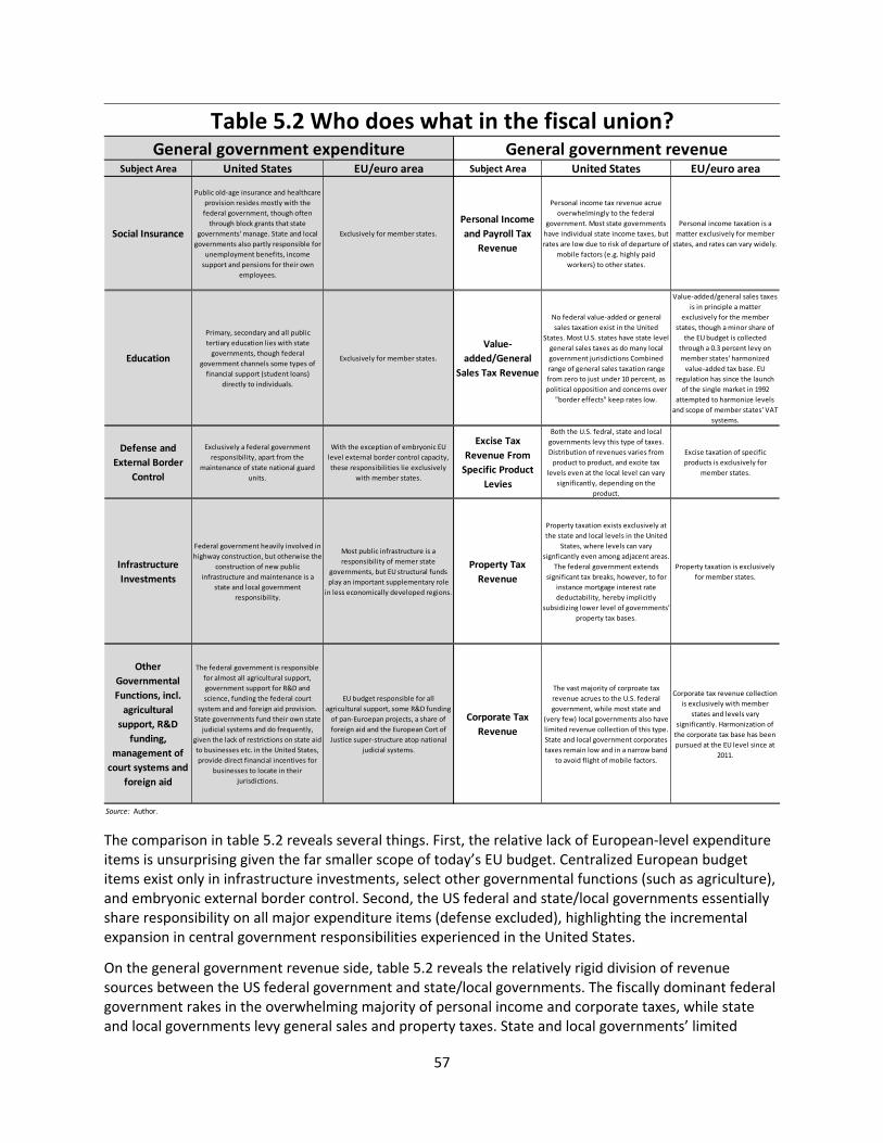
57  

 

The comparison in table 5.2 reveals several things. First, the relative lack of European‐level expenditure items is unsurprising given the far smaller scope of today’s EU budget. Centralized European budget items exist only in infrastructure investments, select other governmental functions (such as agriculture), and embryonic external border control. Second, the US federal and state/local governments essentially share responsibility on all major expenditure items (defense excluded), highlighting the incremental expansion in central government responsibilities experienced in the United States.  

On the general government revenue side, table 5.2 reveals the relatively rigid division of revenue sources between the US federal government and state/local governments. The fiscally dominant federal government rakes in the overwhelming majority of personal income and corporate taxes, while state and local governments levy general sales and property taxes. State and local governments’ limited 

Subject Area United States EU/euro area Subject Area United States EU/euro area

Social Insurance

Public old‐age insurance and healthcare 

provision resides mostly with the 

federal government, though often 

through block grants that state 

governments' manage. State and local 

governments also partly responsible for 

unemployment benefits, income 

support and pensions for their own 

employees.

Exclusively for member states.

Personal Income 

and Payroll Tax 

Revenue

Personal income tax revenue acrue 

overwhelmingly to the federal 

government. Most state governments 

have individual state income taxes, but 

rates are low due to risk of departure of 

mobile factors (e.g. highly paid 

workers) to other states.

Personal income taxation is a 

matter exclusively for member 

states, and rates can vary widely.

Education

Primary, secondary and all public 

tertiary education lies with state 

governments, though federal 

government channels some types of 

financial support (student loans) 

directly to individuals.

Exclusively for member states.

Value‐

added/General 

Sales Tax Revenue

No federal value‐added or general 

sales taxation exist in the United 

States. Most U.S. states have state level 

general sales taxes as do many local 

government jurisdictions Combined 

range of general sales taxation range 

from zero to just under 10 percent, as 

political opposition and concerns over 

"border effects" keep rates low.

Value‐added/general sales taxes 

is in principle a matter 

exclusively for the member 

states, though a minor share of 

the EU budget is collected 

through a 0.3 percent levy on 

member states' harmonized 

value‐added tax base. EU 

regulation has since the launch 

of the single market in 1992 

attempted to harmonize levels 

and scope of member states' VAT 

systems.

Defense and 

External Border 

Control

Exclusively a federal government 

responsibility, apart from the 

maintenance of state national guard 

units.

With the exception of embryonic EU 

level external border control capacity, 

these responsibilities lie exclusively 

with member states.

Excise Tax 

Revenue From 

Specific Product 

Levies

Both the U.S. fedral, state and local 

governments levy this type of taxes. 

Distribution of revenues varies from 

product to product, and excite tax 

levels even at the local level can vary 

significantly, depending on the 

product.

Excise taxation of specific 

products is exclusively for 

member states.

Infrastructure 

Investments

Federal government heavily involved in 

highway construction, but otherwise the 

construction of new public 

infrastructure and maintenance is a 

state and local government 

responsibility.

Most public infrastructure is a 

responsibility of memer state 

governments, but EU structural funds 

play an important supplementary role 

in less economically developed regions.

Property Tax 

Revenue

Property taxation exists exclusively at 

the state and local levels in the United 

States, where levels can vary 

signficantly even among adjacent areas. 

The federal government extends 

significant tax breaks, however, to for 

instance mortgage interest rate 

deductability, hereby implicitly 

subsidizing lower level of governments' 

property tax bases.

Property taxation is exclusively 

for member states.

Other 

Governmental 

Functions, incl. 

agricultural 

support, R&D 

funding, 

management of 

court systems and 

foreign aid

The federal government is responsible 

for almost all agricultural support, 

government support for R&D and 

science, funding the federal court 

system and and foreign aid provision. 

State governments fund their own state 

judicial systems and do frequently, 

given the lack of restrictions on state aid 

to businesses etc. in the United States, 

provide direct financial incentives for 

businesses to locate in their 

jurisdictions.

EU budget responsible for all 

agricultural support, some R&D funding 

of pan‐Euroepan projects, a share of 

foreign aid and the European Cort of 

Justice super‐structure atop national 

judicial systems.

Corporate Tax 

Revenue

The vast majority of corproate tax 

revenue acrues to the U.S. federal 

government, while most state and 

(very few) local governments also have 

limited revenue collection of this type. 

State and local government corporates 

taxes remain low and in a narrow band 

to avoid flight of mobile factors. 

Corporate tax revenue collection 

is exclusively with member 

states and levels vary 

significantly. Harmonization of 

the corporate tax base has been 

pursued at the EU level since at 

2011.

Source:  Author.

General government expenditure

Table 5.2 Who does what in the fiscal union?General government revenue

58  

imposition of personal income and corporate taxes remains highly range‐bound, due to the fears of creating border effects in the integrated US national economy. The same functional logic of the gradual harmonization of some of member states’ tax provisions pursued by the European Commission has played out among US states in a single, more cohesive economic unit.  

The one noticeable exception from these findings is in the category of specific excise taxes. Both the US federal government and state/local governments habitually levy these on different individual product categories and often, as with sin and fuel taxes, at the same time. Specific state and local government excise taxes moreover frequently vary widely from those of neighboring jurisdictions. As highlighted in Part II, such specific taxes and levies enable the US general government budget practice of earmarked funding, where new revenues are collected to pay for specific budget expenditures. As argued later, this is a promising new budget practice also for the European Union or euro area to embrace as it seeks to grow the scope of its common budget. 

The political ability to fund specific spending priorities with earmarked revenue moreover generally facilitates the incremental growth of the central US government budget. Conscious political decisions (often in times of crisis) have generally driven the expansion of the US federal government one policy area at a time, and it has historically made political sense in the United States to often also consider how to independently fund new government initiatives or programs. The ability to secure political acceptance of more federal government revenue by directly tying its collection to intended expenditure items though earmarked tax revenues has often been crucial. Limiting central government discretion over how to spend new revenue has facilitated the growth of the federal government’s budget. 

The US fiscal union’s growth path also highlights the importance of sequencing in the budgetary growth process, as political agreement on which things new federal government expenditure should fund always preceded the political decision on which tools to rely on to collect the required federal government revenue. US experiences thus clearly highlight how policymakers continuously must evaluate which challenges the central government should tackle (e.g., EU or euro area level) and what is best left to (member) states. Just like US states’ rights concerns shift over time, so too will the outcome of the functionally equivalent European subsidiarity principle. The sudden onslaught of the Great Depression and collapse of the embryonic state safety nets made it an urgent political and economic necessity for the federal government to begin to provide generally available old‐age pensions and unemployment benefits in the United States. No other level of American government could have borne this burden at that critical point in time.  

The deepest US political and economic crises have all demanded an institutional governance response, and most often so led by the federal government in collaboration with state (and local) governments. 

   

59  

Part II  Elements of the Modern US Federal Government Most Relevant to EU Policymaking   No government ever voluntarily reduces itself in size. Government programs, once launched, never disappear.  

  —Ronald Reagan44 

Part II analyzes the origins and functions of seven institutions from the present‐day US fiscal union that are particularly relevant for euro area policymakers at this point in time. These are the US unemployment insurance system; earmarked revenue and trust fund budgeting; the federal Highway Trust Fund; US states’ rainy day funds; issuance of state and local government debt; US states’ balanced budget provisions; and competitively distributed federal government TIGER grants to states. 

 

6 US Unemployment Compensation: A Unique State and Federal Government Social Insurance Program Collaboration 

The 1935 Social Security Act (SSA) for the first time created a broad‐based unemployment insurance program in the United States. The federal/state unemployment insurance system (UI) is intended to assist people who have temporarily lost their jobs by providing benefits while they search for work. It is funded through payroll taxes levied on employers, as well as in a few states on employees too. 

The actual unemployment insurance programs are run by the states, which collect taxes from employers and disburse benefits to workers. The federal government pays only the administrative costs via earmarked federal payroll taxes on workers, and the US Department of Labor monitors states’ compliance with federal law. 

From the beginning, the Roosevelt administration intended that “[t]he States shall have broad freedom to set up the type of unemployment compensation they wish,”45 so federal law makes only limited demands on state UI laws, focusing on ensuring minimal protection for eligible workers and making sure the system acts as a countercyclical buffer during economic downturns.  

Labor market regulations, certainly by European standards, are very limited in US states and are generally similar across all states. This is partly the reason for limited federal interference in states’ regulation of UI (and other elements of labor market regulation). In other words, the federal government has no real reason to impose any material compliance requirements on states for being part of the federal UI system. The uniformly limited regulation of labor markets in the United States makes such a requirement superfluous, as the degree of variance among states at their very low average level of labor market regulation has only a limited and at most sector‐specific impact on labor market 

                                                            44 See https://www.brainyquote.com/quotes/quotes/r/ronaldreag147680.html  45 See Perkins (1935). 

60  

outcomes.46 An indicative measure of relative nonvariation in regional US labor market outcomes is state‐level unemployment rates. Their range even during the depth of the Great Recession and its aftermath exceeded more than 11 percentage points only once in the month of July 200947 and typically is in the range of 5 percentage points around the US national full employment level.48 

In the case of the euro area or European Union, the very wide discrepancies between member states’ labor market regulations and corresponding differences in labor market outcomes in terms of, for instance, unemployment rates,49 prevalence of long‐term unemployment,50 or activity rates51 means any European‐level unemployment insurance scheme would have to be designed differently than the US UI system. Given the large differences in labor market performance in Europe, eligibility would likely have to be conditioned on member state compliance with a sizable number of legal statutory requirements in European law. The reality of greatly differing labor market outcomes in Europe hence will make it politically much harder to uniformly insure European unemployed even partly at the European level. 

Unemployment benefits in the United States are defined as simply “cash benefits payable to individuals with respect to their unemployment.”52 States are prohibited from taking money out of the state unemployment fund managed by the federal government for purposes other than paying unemployment benefits, and are—to ensure broad access to benefits for all groups of workers53— banned from utilizing too burdensome administrative methods in establishing workers’ eligibility for benefits. Workers must have lost their job through no fault of their own, be actively looking for work, and have held some sort of prior employment. In other words, US UI by design does not cover workers who voluntarily left a job, first‐time job seekers, or workers rejoining the labor force after a period of voluntary inactivity. 

6.1 Variation in State Unemployment Regulations 

Within the basic federal government legal framework, states can choose their own desired level of employer taxes, benefit levels and duration, and worker benefit eligibility criteria such as duration and character of previous employment record. Consequently, basic elements of states’ UI programs vary considerably across states. Table 6.1 presents the maximum levels of benefits and duration in the 50 US states, the District of Columbia, and territory of Puerto Rico. 

                                                            46 For more details on US labor market regulation, see the country‐specific explanation of the US score in the OECD’s Employment Protection Legislation (EPL) rankings in OECD (2013). 47 That month Michigan had an unemployment rate of 15.3 percent and North Dakota 3.9 percent. 48 Data from the Bureau of Labor Statistics at www.bls.gov/lau/data.htm.  49 In the European Union, the range of member state unemployment rates has exceeded 20 percentage points since July 2012. 50 In 2016, for instance, only 18 percent of unemployed in Sweden had been without a job for more than 12 months, while that level was almost three times as high at 57 percent in Italy, 59 percent in Bulgaria, and 60 percent in Slovakia. In the European Union and euro area in 2016 the corresponding figures were 7 and 50 percent, respectively. Data from Eurostat at http://ec.europa.eu/eurostat/data/database.  51 Activity rates in the European Union in 2016 ranged between a low of 56.2 percent in Greece and 61.6 percent in Italy to 81.2 percent in Sweden and 78.6 percent in Germany. Data from Eurostat at http://ec.europa.eu/eurostat/data/database.  52 Section 3306(h) of the Federal Unemployment Tax Act, available at www.law.cornell.edu/uscode/text/26/3306.  53 Throughout history southern US states extensively used various administrative measures in a racially discriminatory manner to deny otherwise eligible African‐American workers access to public unemployment benefits. 

61  

 

The vast majority of states offer unemployment benefits for 26 weeks, though eight states less than that and North Carolina in some cases as little as five weeks. Massachusetts is the only state that provides more at 30 weeks. Until the Great Recession hit, long‐term unemployment was relatively rare in the United States, as typically at least 80 percent of US unemployed found a new job within six months (e.g., 

State Maximum Weekly Benefit Amount

Maximum Duration of 

State Unemployment 

Benefits

State Unemployment Insurance Benefits Website for 

Additional Information

Alabama $265  26 Alabama Unemployment Information

Alaska $370  26 Alaska Unemployment Insurance State Website

Arizona $240  26 Arizona Department of Economic Security

Arkansas $451  20 Arkansas Department of Workforce Services

California $450  26 CA.gov EDD details

Colorado $568  26 Colorado Department of Labor and Employment

Connecticut $598  26 Connecticut Department of Labor

Delaware $330  26 Delaware Division of Unemployment Insurance

District of Columbia $425  26 DC Dept. of Employment Services

Florida $275  12 Florida Department of Economic Opportunity

Georgia $330  14 to 20 GA Department of Labor

Hawaii $551  26 Hawaii Unemployment Insurance State Website

Idaho $410  26 Idaho Dept. of Labor

Illinois $449 (Individual) to $613 (w/dependents) 26 IL Unemployment Insurance State Website

Indiana $390  26 Indiana Department of Workforce Development

Iowa $447 (Individual) to $548 (w/dependents) 26 Iowa Workforce Development

Kansas $474  16 Kansas Department of Labor

Kentucky $415  26 Kentucky Career Center

Louisiana $247  26 Louisiana Workforce Commission

Maine $410  26 Maine Department of Labor

Maryland $430  26 MD Department of Labor (DLLR)

Massachusetts $742 + $25 per child 30 MA Labor and Workforce Development

Michigan $362 (w/dependents) 20 Michigan UIA

Minnesota $683  26 MN Department of Employment and Economic Development

Mississippi $235  26 MS Department of Employment Security

Missouri $320  20 MO Department of Labor and Industrial Relations

Montana $487  26 MT Department of Labor and Industry

Nebraska $392  26 NE Department of Labor

Nevada $407  26 NV Dept. of Employment, Training and Rehab

New Hampshire $427  26 NH Department of Employment Security

New Jersey $677  26 NJ Dept. of Labor and Workforce Development

New Mexico $425  26 NM Department of Workforce Solutions

New York $430  26 NY Dept. of Labor

North Carolina $350  5 to 20 NC Division of Employment Security

North Dakota $633  26 ND Job Service

Ohio $435 (Individual) to $587 (w/dependents) 26 Ohio Dept. of Job and Family Services

Oklahoma $505  26 Oklahoma UI Home Page

Oregon $590  26 Oregon Employment Department

Pennsylvania $573 + $8 per week for each dependent 26 PA Office of Unemployment Compensation

Rhode Island $566  26 RI Dept. of Labor and Training

South Carolina $326  20 SC Dept. of Employment & Workforce

South Dakota $345  26 SD Department of Labor & Regulation

Tennessee $275  26 TN Dept. of Labor and Workforce Development

Texas $493  26 Texas Workforce Commission

Utah $496  26 Dept. of Workforce Services

Vermont $458  26 VT Dept. of Labor

Virginia $378  26 VA Employment Commission

Washington $681  26 WA Employment Security Department

West Virginia $424  26 West Virginia Unemployment Insurance Page

Wisconsin $370  26 WI Dept. of Workforce Development

Wyoming $471  26 Wyoming Unemployment Insurance Home Page

Addendum:

Puerto Rico $42 to $133 26 PR Department of Labor & HR

Source: US Department of Labor.

Table 6.1  US states' unemployment benefit levels and maximum duration, 2017

62  

long‐term unemployment was 20 percent or less). Most American unemployed in most states therefore traditionally had access to unemployment benefits throughout their unemployment spell, even as many might not be eligible for the maximum duration of unemployment benefits due to short prior work histories. Maximum benefit levels vary considerably across US states, from $235/week in Mississippi to almost $750/week in Massachusetts. Adjusted for state income levels and regional cost of living, most US states aim for a benefit replacement rate of close to 50 percent for maximum benefits during the first six months of unemployment. As will be discussed below, benefit replacement rates typically decline during federally funded emergency unemployment benefit extensions. 

Overall, in comparison to most European unemployment benefit systems, US states provide lower levels of benefits for shorter periods of time. 

The Federal Unemployment Tax Act (FUTA) levies a 6 percent employer payroll tax on the first $7,000 in wages paid to eligible employees. Provided, however, that firms pay state unemployment taxes on time and irrespective of the scale of state UI taxes paid, FUTA provides a 5.4 percent tax credit, leaving most employers to pay only a 0.6 percent effective federal tax, or $42/eligible employee.54 States charge employers varying levels of payroll taxes, in accordance with the financing requirements of their different benefit levels. Only Alaska, New Jersey, and Pennsylvania levy any UI charges on workers, too. Table 6.2 shows the different employer payroll taxes financing state unemployment benefits.  

                                                            54 The size of the tax break may be reduced if a state has a financial obligation to the federal government arising from inability to pay unemployment benefits in a timely manner. 

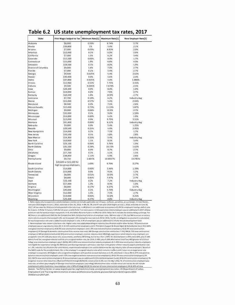
63  

 

Alabama $8,000 0.59% 6.74% 2.7%

Alaska $39,800 1% 5.4% 2.1%

Arizona  $7,000 0.03% 8.91% 2.0%

Arkansas $12,000 0.1% 6.0% 2.9%

California $7,000 1.5% 6.2% 3.4%

Colorado $12,500 0.66% 8.9% 1.7%

Connecticut $15,000 1.9% 6.8% 4.3%

Delaware $18,500 0.1% 8.0% 1.9%

District of Columbia  $9,000 1.6% 7.0% 2.7%

Florida $7,000 0.1% 5.4% 2.7%

Georgia $9,500 0.025% 5.4% 2.62%

Hawaii $40,400 0.0% 5.6% 2.4%

Idaho  $37,800 0.425% 5.4% 1.488%

Ill inois $12,960 0.55% 7.75% 3.55%

Indiana $9,500 0.505% 7.474% 2.5%

Iowa $29,300 0.0% 8.0% 1.0%

Kansas $14,000 0.2% 7.6% 2.7%

Kentucky $10,200 1.0% 10.0% 2.7%

Louisiana $7,700 0.10% 6.2% Industry Avg

Maine $12,000 0.57% 5.4% 2.04%

Maryland $8,500 0.3% 7.5% 2.6%

Massachusetts $15,000 0.73% 11.13% 1.87%

Michigan $9,000 0.06% 10.3% 2.7%

Minnesota $32,000 0.1% 9.0% 1.59%

Mississippi $14,000 0.00% 5.4% 1.0%

Missouri $13,000 0.0% 9.75% 3.51%

Montana $31,400 0.00% 6.12% Industry Avg

Nebraska  $9,000 0.0% 5.4% 1.25%

Nevada $29,500 0.25% 5.4% 2.95%

New Hampshire $14,000 0.1% 7.5% 1.7%

New Jersey $33,500 0.5% 5.8% 2.8%

New Mexico $24,300 0.33% 5.4% Industry Avg

New York $10,900 1.1% 8.5% 3.4%

North Carolina $23,100 0.06% 5.76% 1.0%

North Dakota $35,100 0.28% 10.72% 1.62%

Ohio $9,000 0.3% 8.7% 2.7%

Oklahoma $17,700 0.1% 5.5% 1.5%

Oregon $38,400 1.11% 5.4% 2.6%

Pennsylvania $9,750 2.801% 10.8937% 3.6785%

South Carolina $14,000 0.06% 5.46% 1.39%

South Dakota $15,000 0.0% 9.5% 1.2%

Tennessee $8,000 0.01% 10.0% 2.7%

Texas $9,000 0.45% 7.47% 2.7%

Utah $33,100 0.2% 7.2% Industry Avg

Vermont  $17,300 1.3% 8.4% 1.0%

Virginia $8,000 0.17% 6.27% 2.57%

Washington $45,000 0.1% 5.70% Industry Avg

West Virginia $12,000 1.5% 7.5% 2.7%

Wisconsin $14,000 0.05% 12.0% 3.25%

Wyoming $25,400 0.27% 8.8% Industry Avg

Table 6.2   US state unemployment tax rates, 2017State First Wages Subject to Tax Minimum Rate[1] Maximum Rate[1] New Employer Rate[2]

2. New employer rate shown is the base rate. Higher rates may apply depending on industry classification and/or other factors: DE (construction 

employers pay an avg industry rate); DC; IL (4.15% construction employers and 3.75% Admin Support & Waste Mgmt & Remediation Svcs); IN (1.60% 

new governmental employers); IA (8.0% new construction employers and 1.0% new nonconstruction employers); KS (6.0% new construction 

employers); KY (foreign & domestic construction firms receive max rate); MD (foreign construction contractors 7.5%); MA (6.73% new construction 

employers); ME (predetermined yield); MI (construction employers receive industry rate); MN (high experience rated industry new employers are 

assigned a rate of 9.10% plus base rate, assessments, and fees); MT (InAvg, but no less than 1.00%; for 2016 between 1.00% and 2.60%, plus 0.18% 

Admin Fund Tax; new governmental entities are assigned median rate, for 2016, 0.36%, plus 0.09% Alternative Fund Tax); MO (greater of 3.51% or 

InAvg; new construction employers pay 4.362%); NE (1.00% new nonconstruction industry employers & 5.40% new construction industry employers 

not eligible for experience rating); NJ; NM (new contributing employers will have a rate that is the greater of their industry avg UI contribution rate 

or 1.0%. Industry classifications for contributory, experienced employers are used to determine the avg industry rates of new employers. Based on 

the NAICS code for the establishment, this is the employer’s assigned industry rate which remains in effect until 2 years as an experience rate 

employer is acquired.); NY (highest rate assigned to employers with positive account balances or 3.4%, whichever is less); ND (1.07% new positive‐

balance nonconstruction employers and 6.10% new negative‐balance nonconstruction employers); OH (6.4% new construction employers); PA 

(10.1947% new construction employers); RI (new employers pay an additional 0.21% Job Development Fund); SD (6.0% construction employers); TN 

(negative reserve ratio industries effective 07/01/15 through 06/30/16; construction 6.5%; sect 33 mfg. 5.0%); TX; UT (construction employers pay 

max rate, all others pay InAvg%); VT (foreign construction employers pay InAvg); WA (min/max rates include social cost tax but do not include 

employment admin fund rates; new employer rate is 90% of InAvg); WV (8.5% new out‐of‐state construction employers); WI (6.60% all new 

Sources:  Tax Pol icy Center at www.taxpol icycenter.org/statis tics/state‐unemployment‐tax‐rates ; US Department of Labor, 

Employment and Tra ining Administration at www.workforcesecuri ty.doleta.gov/unemploy/content/s igpros/2010‐

2019/January2017.pdf.

Rhode Island$20,600 or $22,100 for 

high tax group employers1.69% 9.79% 2.27%

1. Rates apply only to experience rated employers and do not include applicable non UI taxes, surtaxes, penalties, or surcharges. In most States, 

rate year 2016 begins on Jan 1, 2016, and ends on Dec 31, 2016. In NH, NJ, TN, and VT rate year 2016 begins on July 1, 2016, and ends on June 30, 

2017. All tax rates for 2016 are initially posted in the July issue. In AR (there is an additional assessment of 2.0% for employers having a deficit rate 

for 2 years; 4.0% for 3‐4 years; 6.0% for 5‐6 years; and 8.0% for 7 or more years). In CO experience‐rated employers pay an additional 0.2447 of base 

premium rate for bond principal repayment. In ID, the Admin Reserve Fund is in effect for 2016. Rates for IL include the fund building surcharge. For 

ME there is an additional 0.06% for the Competitive Skills Scholarship Fund on all employer rates. NM max rate is 5.4%, but NM assesses an excess 

claim rate to accounts that exceed 5.4%, not to exceed 1.0% raising the max rate to 6.4% for 2016. For MI, an obligation assessment is calculated 

for each experience rate and is added to each employer’s rate. In RI all employers pay an additional 0.21% for the job development fund.

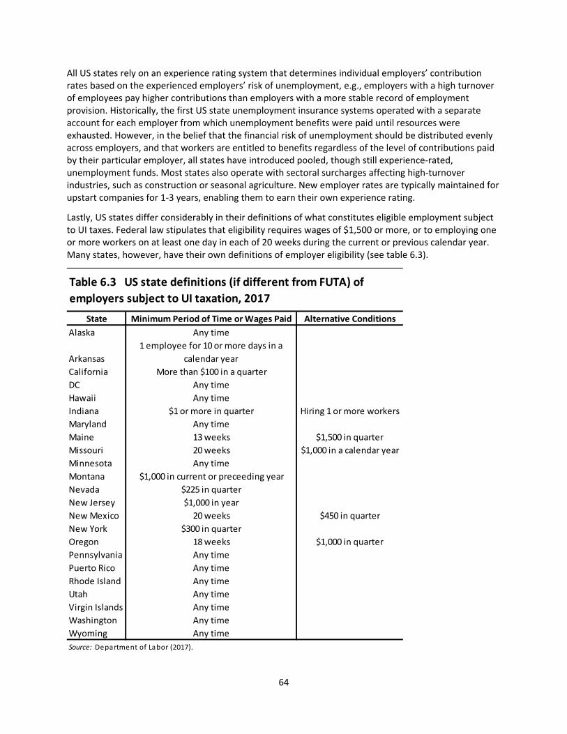
64  

All US states rely on an experience rating system that determines individual employers’ contribution rates based on the experienced employers’ risk of unemployment, e.g., employers with a high turnover of employees pay higher contributions than employers with a more stable record of employment provision. Historically, the first US state unemployment insurance systems operated with a separate account for each employer from which unemployment benefits were paid until resources were exhausted. However, in the belief that the financial risk of unemployment should be distributed evenly across employers, and that workers are entitled to benefits regardless of the level of contributions paid by their particular employer, all states have introduced pooled, though still experience‐rated, unemployment funds. Most states also operate with sectoral surcharges affecting high‐turnover industries, such as construction or seasonal agriculture. New employer rates are typically maintained for upstart companies for 1‐3 years, enabling them to earn their own experience rating. 

Lastly, US states differ considerably in their definitions of what constitutes eligible employment subject to UI taxes. Federal law stipulates that eligibility requires wages of $1,500 or more, or to employing one or more workers on at least one day in each of 20 weeks during the current or previous calendar year. Many states, however, have their own definitions of employer eligibility (see table 6.3). 

 

State Minimum Period of Time or Wages Paid Alternative Conditions

Alaska Any time

Arkansas

1 employee for 10 or more days in a 

calendar year

California More than $100 in a quarter

DC Any time

Hawaii Any time

Indiana $1 or more in quarter Hiring 1 or more workers

Maryland Any time

Maine 13 weeks $1,500 in quarter

Missouri 20 weeks $1,000 in a calendar year

Minnesota Any time

Montana $1,000 in current or preceeding year

Nevada $225 in quarter

New Jersey $1,000 in year

New Mexico 20 weeks $450 in quarter

New York $300 in quarter

Oregon 18 weeks $1,000 in quarter

Pennsylvania Any time

Puerto Rico Any time

Rhode Island Any time

Utah Any time

Virgin Islands Any time

Washington Any time

Wyoming Any time

Source: Department of Labor (2017).

Table 6.3   US state definitions (if different from FUTA) of 

employers subject to UI taxation, 2017

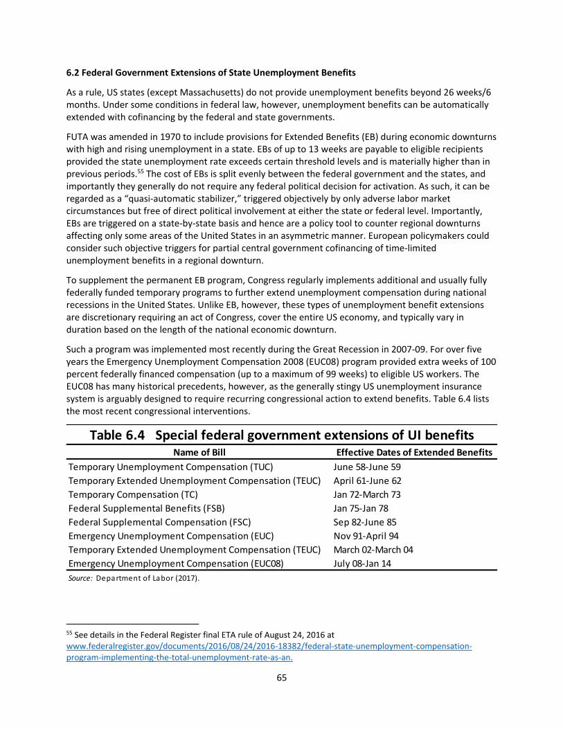
65  

6.2 Federal Government Extensions of State Unemployment Benefits 

As a rule, US states (except Massachusetts) do not provide unemployment benefits beyond 26 weeks/6 months. Under some conditions in federal law, however, unemployment benefits can be automatically extended with cofinancing by the federal and state governments.  

FUTA was amended in 1970 to include provisions for Extended Benefits (EB) during economic downturns with high and rising unemployment in a state. EBs of up to 13 weeks are payable to eligible recipients provided the state unemployment rate exceeds certain threshold levels and is materially higher than in previous periods.55 The cost of EBs is split evenly between the federal government and the states, and importantly they generally do not require any federal political decision for activation. As such, it can be regarded as a “quasi‐automatic stabilizer,” triggered objectively by only adverse labor market circumstances but free of direct political involvement at either the state or federal level. Importantly, EBs are triggered on a state‐by‐state basis and hence are a policy tool to counter regional downturns affecting only some areas of the United States in an asymmetric manner. European policymakers could consider such objective triggers for partial central government cofinancing of time‐limited unemployment benefits in a regional downturn. 

To supplement the permanent EB program, Congress regularly implements additional and usually fully federally funded temporary programs to further extend unemployment compensation during national recessions in the United States. Unlike EB, however, these types of unemployment benefit extensions are discretionary requiring an act of Congress, cover the entire US economy, and typically vary in duration based on the length of the national economic downturn. 

Such a program was implemented most recently during the Great Recession in 2007‐09. For over five years the Emergency Unemployment Compensation 2008 (EUC08) program provided extra weeks of 100 percent federally financed compensation (up to a maximum of 99 weeks) to eligible US workers. The EUC08 has many historical precedents, however, as the generally stingy US unemployment insurance system is arguably designed to require recurring congressional action to extend benefits. Table 6.4 lists the most recent congressional interventions. 

 

                                                            55 See details in the Federal Register final ETA rule of August 24, 2016 at www.federalregister.gov/documents/2016/08/24/2016‐18382/federal‐state‐unemployment‐compensation‐program‐implementing‐the‐total‐unemployment‐rate‐as‐an.  

Name of Bill Effective Dates of Extended Benefits

Temporary Unemployment Compensation (TUC) June 58‐June 59

Temporary Extended Unemployment Compensation (TEUC) April 61‐June 62

Temporary Compensation (TC) Jan 72‐March 73

Federal Supplemental Benefits (FSB) Jan 75‐Jan 78

Federal Supplemental Compensation (FSC) Sep 82‐June 85

Emergency Unemployment Compensation (EUC) Nov 91‐April 94

Temporary Extended Unemployment Compensation (TEUC) March 02‐March 04

Emergency Unemployment Compensation (EUC08)  July 08‐Jan 14

Source:  Department of Labor (2017).

Table 6.4   Special federal government extensions of UI benefits

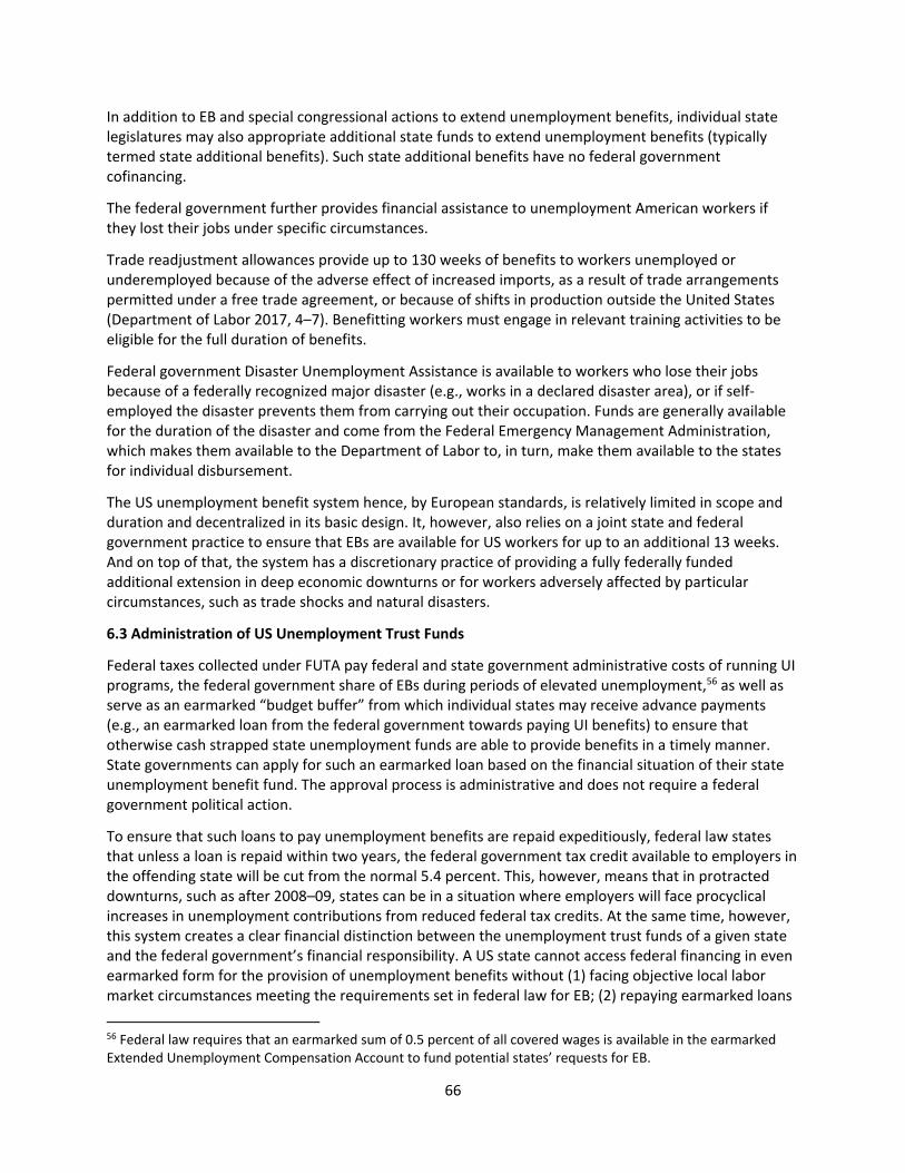
66  

In addition to EB and special congressional actions to extend unemployment benefits, individual state legislatures may also appropriate additional state funds to extend unemployment benefits (typically termed state additional benefits). Such state additional benefits have no federal government cofinancing. 

The federal government further provides financial assistance to unemployment American workers if they lost their jobs under specific circumstances.  

Trade readjustment allowances provide up to 130 weeks of benefits to workers unemployed or underemployed because of the adverse effect of increased imports, as a result of trade arrangements permitted under a free trade agreement, or because of shifts in production outside the United States (Department of Labor 2017, 4–7). Benefitting workers must engage in relevant training activities to be eligible for the full duration of benefits. 

Federal government Disaster Unemployment Assistance is available to workers who lose their jobs because of a federally recognized major disaster (e.g., works in a declared disaster area), or if self‐employed the disaster prevents them from carrying out their occupation. Funds are generally available for the duration of the disaster and come from the Federal Emergency Management Administration, which makes them available to the Department of Labor to, in turn, make them available to the states for individual disbursement. 

The US unemployment benefit system hence, by European standards, is relatively limited in scope and duration and decentralized in its basic design. It, however, also relies on a joint state and federal government practice to ensure that EBs are available for US workers for up to an additional 13 weeks. And on top of that, the system has a discretionary practice of providing a fully federally funded additional extension in deep economic downturns or for workers adversely affected by particular circumstances, such as trade shocks and natural disasters.  

6.3 Administration of US Unemployment Trust Funds 

Federal taxes collected under FUTA pay federal and state government administrative costs of running UI programs, the federal government share of EBs during periods of elevated unemployment,56 as well as serve as an earmarked “budget buffer” from which individual states may receive advance payments (e.g., an earmarked loan from the federal government towards paying UI benefits) to ensure that otherwise cash strapped state unemployment funds are able to provide benefits in a timely manner. State governments can apply for such an earmarked loan based on the financial situation of their state unemployment benefit fund. The approval process is administrative and does not require a federal government political action. 

To ensure that such loans to pay unemployment benefits are repaid expeditiously, federal law states that unless a loan is repaid within two years, the federal government tax credit available to employers in the offending state will be cut from the normal 5.4 percent. This, however, means that in protracted downturns, such as after 2008–09, states can be in a situation where employers will face procyclical increases in unemployment contributions from reduced federal tax credits. At the same time, however, this system creates a clear financial distinction between the unemployment trust funds of a given state and the federal government’s financial responsibility. A US state cannot access federal financing in even earmarked form for the provision of unemployment benefits without (1) facing objective local labor market circumstances meeting the requirements set in federal law for EB; (2) repaying earmarked loans 

                                                            56 Federal law requires that an earmarked sum of 0.5 percent of all covered wages is available in the earmarked Extended Unemployment Compensation Account to fund potential states’ requests for EB. 

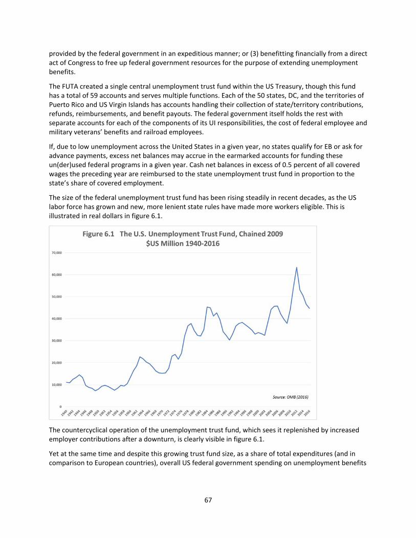
67  

provided by the federal government in an expeditious manner; or (3) benefitting financially from a direct act of Congress to free up federal government resources for the purpose of extending unemployment benefits. 

The FUTA created a single central unemployment trust fund within the US Treasury, though this fund has a total of 59 accounts and serves multiple functions. Each of the 50 states, DC, and the territories of Puerto Rico and US Virgin Islands has accounts handling their collection of state/territory contributions, refunds, reimbursements, and benefit payouts. The federal government itself holds the rest with separate accounts for each of the components of its UI responsibilities, the cost of federal employee and military veterans’ benefits and railroad employees. 

If, due to low unemployment across the United States in a given year, no states qualify for EB or ask for advance payments, excess net balances may accrue in the earmarked accounts for funding these un(der)used federal programs in a given year. Cash net balances in excess of 0.5 percent of all covered wages the preceding year are reimbursed to the state unemployment trust fund in proportion to the state’s share of covered employment. 

The size of the federal unemployment trust fund has been rising steadily in recent decades, as the US labor force has grown and new, more lenient state rules have made more workers eligible. This is illustrated in real dollars in figure 6.1. 

 

The countercyclical operation of the unemployment trust fund, which sees it replenished by increased employer contributions after a downturn, is clearly visible in figure 6.1.  

Yet at the same time and despite this growing trust fund size, as a share of total expenditures (and in comparison to European countries), overall US federal government spending on unemployment benefits 

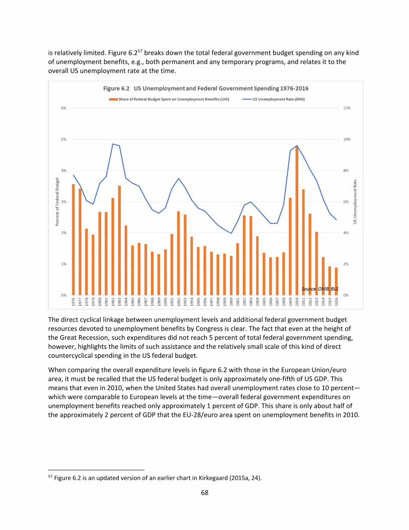
68  

is relatively limited. Figure 6.257 breaks down the total federal government budget spending on any kind of unemployment benefits, e.g., both permanent and any temporary programs, and relates it to the overall US unemployment rate at the time. 

 

The direct cyclical linkage between unemployment levels and additional federal government budget resources devoted to unemployment benefits by Congress is clear. The fact that even at the height of the Great Recession, such expenditures did not reach 5 percent of total federal government spending, however, highlights the limits of such assistance and the relatively small scale of this kind of direct countercyclical spending in the US federal budget.  

When comparing the overall expenditure levels in figure 6.2 with those in the European Union/euro area, it must be recalled that the US federal budget is only approximately one‐fifth of US GDP. This means that even in 2010, when the United States had overall unemployment rates close to 10 percent—which were comparable to European levels at the time—overall federal government expenditures on unemployment benefits reached only approximately 1 percent of GDP. This share is only about half of the approximately 2 percent of GDP that the EU‐28/euro area spent on unemployment benefits in 2010. 

 

   

                                                            57 Figure 6.2 is an updated version of an earlier chart in Kirkegaard (2015a, 24). 

69  

6.4 Conclusion 

The United States has a unique federal‐state collaborative unemployment benefit system, which aims at typically replacing up to about half of workers’ earnings for up to six months, but with some variation among states. Within a broad federal legal framework, variation exists among state rules for benefit levels and duration, employer tax levels, and eligibility. At the same time, it is important to recall that the generally very low level of labor market regulation in the United States means that variation in labor market regulation and outcomes among US states is quite low. This uniformly low level of overall regulation greatly facilitates “light touch” federal regulation of the state‐run unemployment insurance schemes. 

Of particular relevance to European policymakers is the fact that the US federal‐state unemployment benefit system allows for space for individual states to set their own individual unemployment benefit rules and regulations. In normal economic times, the US unemployment benefit system is moreover designed to essentially be a matter for the states to run with only limited administrative help from the federal government. Only in times of economic crises and elevated levels of unemployment does the federal government step in with a direct financial “helping hand” to ensure that unemployed Americans have access to benefits for (more/most of) the duration of the economic downturn.  

US federal government financial involvement in the US unemployment insurance system is hence largely supplementary and is in many ways a step‐by‐step central fiscal backstop to states’ own lean unemployment benefits systems. First, based on objective labor market circumstances in individual states, it includes the ability to cofinance additional unemployment benefits with individual states for a limited duration. Then it allows for the extension of federal government earmarked loans to enable cash‐strapped state‐level unemployment funds to continue to function in economic downturns. And finally Congress regularly releases federal money to nationally extend unemployment benefits further, should economic circumstances dictate it. 

This degree of central continental‐level involvement in countercyclical unemployment benefit provision is hardly impossible to imagine also in the euro area or European Union.  

7 US States and Earmarked Revenues: Novel Ways to Raise Government Resources in Tax‐Hostile Jurisdictions 

Brexit and a host of new European policy challenges are compelling EU leaders to consider overhauling the revenue side of the European Union’s existing budget. This section argues that to create a larger, simpler, more transparent, and therefore more democratically accountable budget, European leaders ought to embrace what in the United States is called “trust fund accounting,” e.g., the earmarking of specifically collected government revenues towards specific identified expenditure items. This will ameliorate public—and therefore member state government—hostility towards raising more direct revenue for the EU budget. Reliable, transparent, and more flexible budget revenue will enable the European Union, or smaller subgroups of member states like the euro area or Schengen Area members, to better respond to ongoing economic, social, and political developments and events in Europe and the world. 

This section first describes how the existing EU budget operates and how it is similar to the US federal budgets of earlier eras. Then it discusses what public goods a centralized budget could/should deliver. Finally, it describes how US state budget practices can inspire possible new EU budget reforms in the future. 

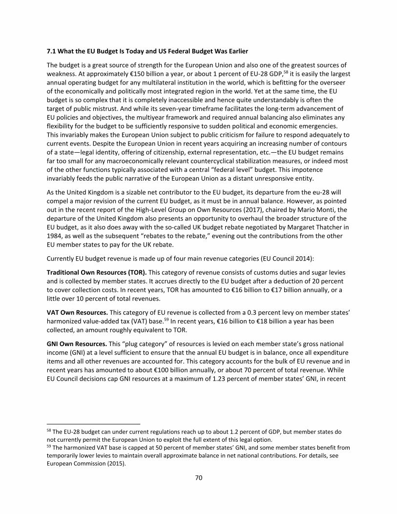
70  

7.1 What the EU Budget Is Today and US Federal Budget Was Earlier 

The budget is a great source of strength for the European Union and also one of the greatest sources of weakness. At approximately €150 billion a year, or about 1 percent of EU‐28 GDP,58 it is easily the largest annual operating budget for any multilateral institution in the world, which is befitting for the overseer of the economically and politically most integrated region in the world. Yet at the same time, the EU budget is so complex that it is completely inaccessible and hence quite understandably is often the target of public mistrust. And while its seven‐year timeframe facilitates the long‐term advancement of EU policies and objectives, the multiyear framework and required annual balancing also eliminates any flexibility for the budget to be sufficiently responsive to sudden political and economic emergencies. This invariably makes the European Union subject to public criticism for failure to respond adequately to current events. Despite the European Union in recent years acquiring an increasing number of contours of a state—legal identity, offering of citizenship, external representation, etc.—the EU budget remains far too small for any macroeconomically relevant countercyclical stabilization measures, or indeed most of the other functions typically associated with a central “federal level” budget. This impotence invariably feeds the public narrative of the European Union as a distant unresponsive entity. 

As the United Kingdom is a sizable net contributor to the EU budget, its departure from the eu‐28 will compel a major revision of the current EU budget, as it must be in annual balance. However, as pointed out in the recent report of the High‐Level Group on Own Resources (2017), chaired by Mario Monti, the departure of the United Kingdom also presents an opportunity to overhaul the broader structure of the EU budget, as it also does away with the so‐called UK budget rebate negotiated by Margaret Thatcher in 1984, as well as the subsequent “rebates to the rebate,” evening out the contributions from the other EU member states to pay for the UK rebate. 

Currently EU budget revenue is made up of four main revenue categories (EU Council 2014): 

Traditional Own Resources (TOR). This category of revenue consists of customs duties and sugar levies and is collected by member states. It accrues directly to the EU budget after a deduction of 20 percent to cover collection costs. In recent years, TOR has amounted to €16 billion to €17 billion annually, or a little over 10 percent of total revenues. 

VAT Own Resources. This category of EU revenue is collected from a 0.3 percent levy on member states’ harmonized value‐added tax (VAT) base.59 In recent years, €16 billion to €18 billion a year has been collected, an amount roughly equivalent to TOR. 

GNI Own Resources. This “plug category” of resources is levied on each member state’s gross national income (GNI) at a level sufficient to ensure that the annual EU budget is in balance, once all expenditure items and all other revenues are accounted for. This category accounts for the bulk of EU revenue and in recent years has amounted to about €100 billion annually, or about 70 percent of total revenue. While EU Council decisions cap GNI resources at a maximum of 1.23 percent of member states’ GNI, in recent 

                                                            58 The EU‐28 budget can under current regulations reach up to about 1.2 percent of GDP, but member states do not currently permit the European Union to exploit the full extent of this legal option. 59 The harmonized VAT base is capped at 50 percent of member states’ GNI, and some member states benefit from temporarily lower levies to maintain overall approximate balance in net national contributions. For details, see European Commission (2015). 

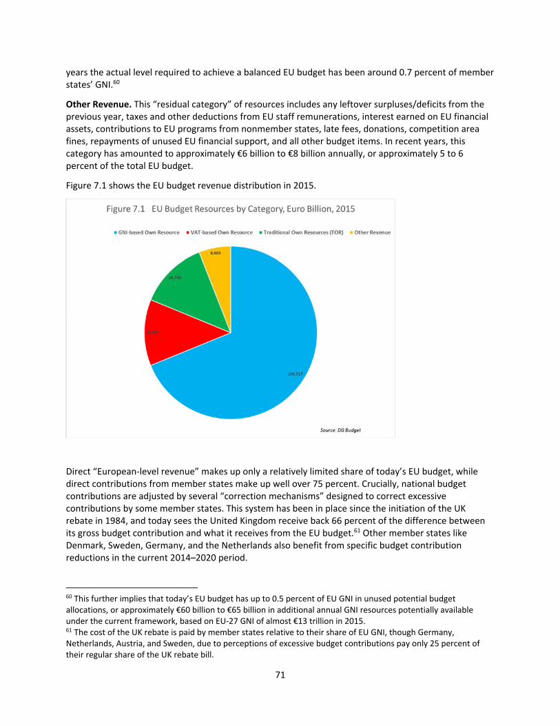
71  

years the actual level required to achieve a balanced EU budget has been around 0.7 percent of member states’ GNI.60 

Other Revenue. This “residual category” of resources includes any leftover surpluses/deficits from the previous year, taxes and other deductions from EU staff remunerations, interest earned on EU financial assets, contributions to EU programs from nonmember states, late fees, donations, competition area fines, repayments of unused EU financial support, and all other budget items. In recent years, this category has amounted to approximately €6 billion to €8 billion annually, or approximately 5 to 6 percent of the total EU budget. 

Figure 7.1 shows the EU budget revenue distribution in 2015. 

 

 

Direct “European‐level revenue” makes up only a relatively limited share of today’s EU budget, while direct contributions from member states make up well over 75 percent. Crucially, national budget contributions are adjusted by several “correction mechanisms” designed to correct excessive contributions by some member states. This system has been in place since the initiation of the UK rebate in 1984, and today sees the United Kingdom receive back 66 percent of the difference between its gross budget contribution and what it receives from the EU budget.61 Other member states like Denmark, Sweden, Germany, and the Netherlands also benefit from specific budget contribution reductions in the current 2014–2020 period. 

                                                            60 This further implies that today’s EU budget has up to 0.5 percent of EU GNI in unused potential budget allocations, or approximately €60 billion to €65 billion in additional annual GNI resources potentially available under the current framework, based on EU‐27 GNI of almost €13 trillion in 2015. 61 The cost of the UK rebate is paid by member states relative to their share of EU GNI, though Germany, Netherlands, Austria, and Sweden, due to perceptions of excessive budget contributions pay only 25 percent of their regular share of the UK rebate bill. 

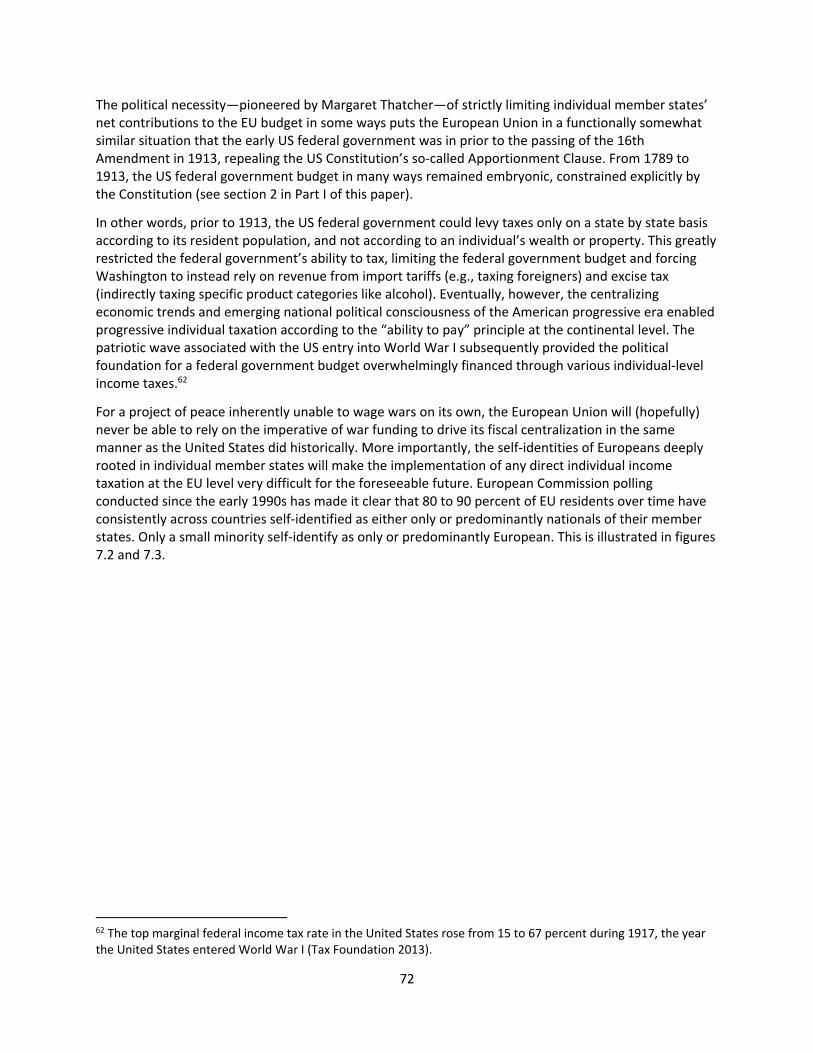
72  

The political necessity—pioneered by Margaret Thatcher—of strictly limiting individual member states’ net contributions to the EU budget in some ways puts the European Union in a functionally somewhat similar situation that the early US federal government was in prior to the passing of the 16th Amendment in 1913, repealing the US Constitution’s so‐called Apportionment Clause. From 1789 to 1913, the US federal government budget in many ways remained embryonic, constrained explicitly by the Constitution (see section 2 in Part I of this paper).  

In other words, prior to 1913, the US federal government could levy taxes only on a state by state basis according to its resident population, and not according to an individual’s wealth or property. This greatly restricted the federal government’s ability to tax, limiting the federal government budget and forcing Washington to instead rely on revenue from import tariffs (e.g., taxing foreigners) and excise tax (indirectly taxing specific product categories like alcohol). Eventually, however, the centralizing economic trends and emerging national political consciousness of the American progressive era enabled progressive individual taxation according to the “ability to pay” principle at the continental level. The patriotic wave associated with the US entry into World War I subsequently provided the political foundation for a federal government budget overwhelmingly financed through various individual‐level income taxes.62 

For a project of peace inherently unable to wage wars on its own, the European Union will (hopefully) never be able to rely on the imperative of war funding to drive its fiscal centralization in the same manner as the United States did historically. More importantly, the self‐identities of Europeans deeply rooted in individual member states will make the implementation of any direct individual income taxation at the EU level very difficult for the foreseeable future. European Commission polling conducted since the early 1990s has made it clear that 80 to 90 percent of EU residents over time have consistently across countries self‐identified as either only or predominantly nationals of their member states. Only a small minority self‐identify as only or predominantly European. This is illustrated in figures 7.2 and 7.3. 

 

 

                                                            62 The top marginal federal income tax rate in the United States rose from 15 to 67 percent during 1917, the year the United States entered World War I (Tax Foundation 2013). 

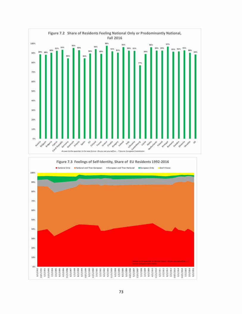
73  

 

 

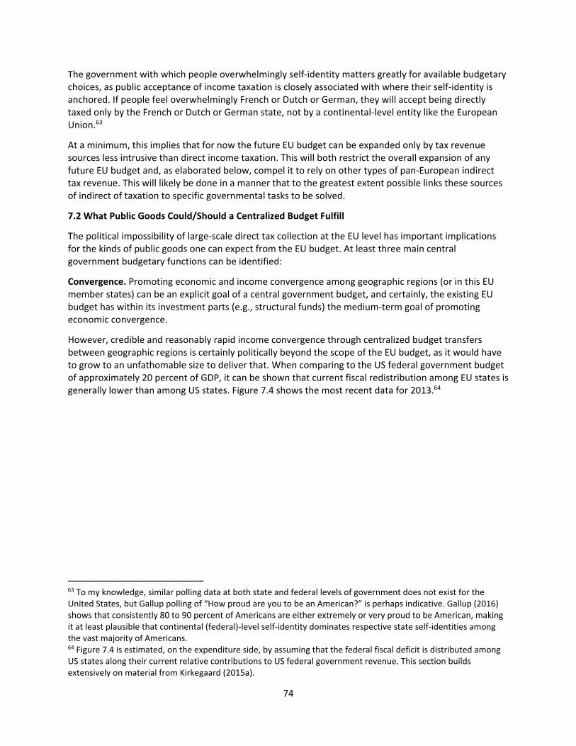
74  

The government with which people overwhelmingly self‐identity matters greatly for available budgetary choices, as public acceptance of income taxation is closely associated with where their self‐identity is anchored. If people feel overwhelmingly French or Dutch or German, they will accept being directly taxed only by the French or Dutch or German state, not by a continental‐level entity like the European Union.63  

At a minimum, this implies that for now the future EU budget can be expanded only by tax revenue sources less intrusive than direct income taxation. This will both restrict the overall expansion of any future EU budget and, as elaborated below, compel it to rely on other types of pan‐European indirect tax revenue. This will likely be done in a manner that to the greatest extent possible links these sources of indirect of taxation to specific governmental tasks to be solved.  

7.2 What Public Goods Could/Should a Centralized Budget Fulfill 

The political impossibility of large‐scale direct tax collection at the EU level has important implications for the kinds of public goods one can expect from the EU budget. At least three main central government budgetary functions can be identified: 

Convergence. Promoting economic and income convergence among geographic regions (or in this EU member states) can be an explicit goal of a central government budget, and certainly, the existing EU budget has within its investment parts (e.g., structural funds) the medium‐term goal of promoting economic convergence.  

However, credible and reasonably rapid income convergence through centralized budget transfers between geographic regions is certainly politically beyond the scope of the EU budget, as it would have to grow to an unfathomable size to deliver that. When comparing to the US federal government budget of approximately 20 percent of GDP, it can be shown that current fiscal redistribution among EU states is generally lower than among US states. Figure 7.4 shows the most recent data for 2013.64 

                                                            63 To my knowledge, similar polling data at both state and federal levels of government does not exist for the United States, but Gallup polling of “How proud are you to be an American?” is perhaps indicative. Gallup (2016) shows that consistently 80 to 90 percent of Americans are either extremely or very proud to be American, making it at least plausible that continental (federal)‐level self‐identity dominates respective state self‐identities among the vast majority of Americans. 64 Figure 7.4 is estimated, on the expenditure side, by assuming that the federal fiscal deficit is distributed among US states along their current relative contributions to US federal government revenue. This section builds extensively on material from Kirkegaard (2015a). 

75  

 

The specific revenue and expenditure responsibilities of any central budget have natural direct net redistributive outcome effects in the same manner that, for instance, the EU budget’s historical focus on agricultural support ipso facto delivers a significant resource stream to France. With the vast majority of US federal government revenue coming from individual income taxes and mandatory employment‐related social contributions and most federal spending going out in direct payments to individual Americans, the scope for geographic fiscal redistribution between US states through the federal budget far exceeds that of the EU budget.  

On the revenue side, federal government proceeds raised in a given state are, due to the progressive nature of the federal income tax, largely dictated by the state’s general level of prosperity. High levels of average state resident incomes equal relatively high levels of payments into the federal budget. Conversely, on average poor US states like West Virginia and Mississippi contribute relatively less and therefore generally are net recipients of federal government resources. On spending, states that have in recent decades seen a large inflow of elderly residents, such as Florida, benefit from a relatively higher inflow of this type of federal fiscal resources. At the same time, the biggest geographic impact of where federal money is spent comes through the location of federal government facilities, and noticeably US military institutions.65 States with a large number of such government facilities, such as the District of 

                                                            65 Recognizing the economic and political importance of the locations of US military installations, Congress and the Department of Defense have since the end of the Cold War—which precipitated the closure of many such facilities—governed the process through the establishment of an independent Base Closure and Realignment Commission (BRAC). The BRAC, made up of retired general‐rank military personnel, diplomats, and policymakers, is charged with issuing a report to the president on how best to achieve the optimal US military base structure, given 

76  

Columbia, New Mexico, Hawaii, Virginia, Maryland, and Alaska, receive relatively larger inflows of federal resources. 

It is clear from US federal government circumstances that any redistributional budgetary effects tend to be overwhelmingly structural in nature, as they are dictated by long‐term relative income levels, demographic trends, and locational choices for government institutions.  

Countercyclical Budget Buffer. A central budget’s ability to influence the short‐term business cycle, or counter a geographically isolated asymmetric shock, is another important function. In the context of the euro area crisis, it became increasingly obvious that the lack of such budget capacity at the euro area level resulted in materially worse economic developments in several member states. 

Cyclical redistribution through regular budget allocations is, however, inherently difficult as no one knows where or when the next economic downturn will hit. This budgetary function is consequently best carried out through the ability of a central government to go into debt during a downturn. This allows a central government to both continue to fund existing government expenditure despite lower revenue and implement new spending measures targeted at specific economic circumstances of the downturn. The result is a surprisingly limited immediate overlap between a centralized budget’s geographically redistributional effects and its ability to act as a countercyclical buffer.  

In the case of EU budget reform, explicit discussions about centralized debt issuance to cover cyclical expenditure seem politically infeasible for the foreseeable future and without preceding agreement among member states of additional pooling of political sovereignty over fiscal issues. At the same time, however, while pooling of existing member state national debt into fully joint debt (e.g., the standard introduction of Eurobonds) remains highly unlikely for the foreseeable future, prospects for potential issuance of new common debt instruments in the euro area appear better. The intergovernmental ESM of course already issues centralized (but not fully mutualized) debt conditionally available to member states in financial rescue programs, and initial feasibility discussions have begun at the European Systemic Risk Board (ESRB) on the creation of a new European safe asset.66 

Important centralized cyclical stabilization functions are at the same time carried out by institutions other than the central budget. Most important of these is the fee‐based financing of central rescue/resolution funds for failing banks. In the United States, this is done by the FDIC, a set‐up that in time will be largely replicated by the EU banking union. Critically though, the FDIC today has an explicit legislated access to up to $100 billion from the US Treasury, a level that during the crisis in 2009–10 rose to a potential $500 billion.  

In practice, in the EU/euro area institutional framework, this kind of fiscal backstop for bank rescue/resolution funds is provided by the intergovernmental ESM (in addition to funding national or sector‐specific financial sector rescues), rather than by the regular EU budget or the still missing full fiscal backstop to the emerging industry‐funded Single Resolution Fund (SRF). Until the banking union institutional structure is complete with a fully funded SRF and an FDIC‐like fiscal backstop for systemic crises, the cyclical stabilization achieved through orderly European bank rescues/restructurings/resolutions funded by a centralized entity will be jeopardized by the inherent political conditionality attached to any ESM financing and the fact that ESM activities are generally 

                                                            the tasks and challenges facing the Department of Defense. There have been six BRAC processes since the late 1980s. 66 The ESRB has created a High‐Level Task Force on Safe Assets with the mandate to investigate the potential creation of sovereign bond–backed securities (SBSs), which could comprise senior and junior claims on a diversified portfolio of sovereign bonds. See www.esrb.europa.eu/news/pr/date/2016/html/pr160929.en.html.  

77  

subject to the national vetos of the largest shareholder member states. In all probability, once a crisis of sufficient scale occurred, any required ESM funding would materialize, but without actual precedent to date, no guarantee can be given. It is another bridge Europe will have to cross when it gets there. 

Specific Policy Challenges Best Solved at the Regional Level. The third functional category of public goods delivered by a central budget is the ability to address policy problems best solved at the regional level. The determination of what such policy items are is evidently inherently political and changes over time. Indeed, traditional neofunctional spillover theory of EU integration stipulates that more and more such policy areas will be created as a direct outcome of previous integration effects on adjacent subjects. The gradual historical development of first the EU customs union (e.g., elimination of internal EU tariffs), then the EU internal market (e.g., harmonization of product standards), and finally in parts of the European Union, the common currency is one such example. Addressing climate change or external border control issues are more recent examples of the logic of best regional solutions.  

As discussed in the High‐Level Group on Own Resources (2017) it is critically important that the notion of “EU value added,” e.g., the value of an EU intervention in excess of what would have resulted from member states‐only actions, be considered when EU budget responsibilities are determined. This will offset the reduction of the EU budget to simply being about achieving the politically acceptable range of net balances among member states. 

7.3 Overcoming the Challenges to a Better EU Budget 

The principal challenge to expanding EU budget revenue, and/or making it “more European” and less dependent on direct transfers from naturally hesitant member state governments, is the political impossibility of levying European‐level taxes directly on the individual EU residents. This situation is unlikely to change for the foreseeable future, as Europeans continue to overwhelmingly self‐identify as nationals of their member states, rather than European (figures 7.2 and 7.3).  

Yet, the similar if inverse political reality vin the United States—where the national (e.g., federal) level commands the majority of Americans’ self‐identity and the federal government is hence fiscally dominant—has not prevented state and local governments in the United States from accounting for a very large share of US general government receipts. Figure 7.5 shows the relative developments of federal and state/local government receipts from 1929 to 2016. 

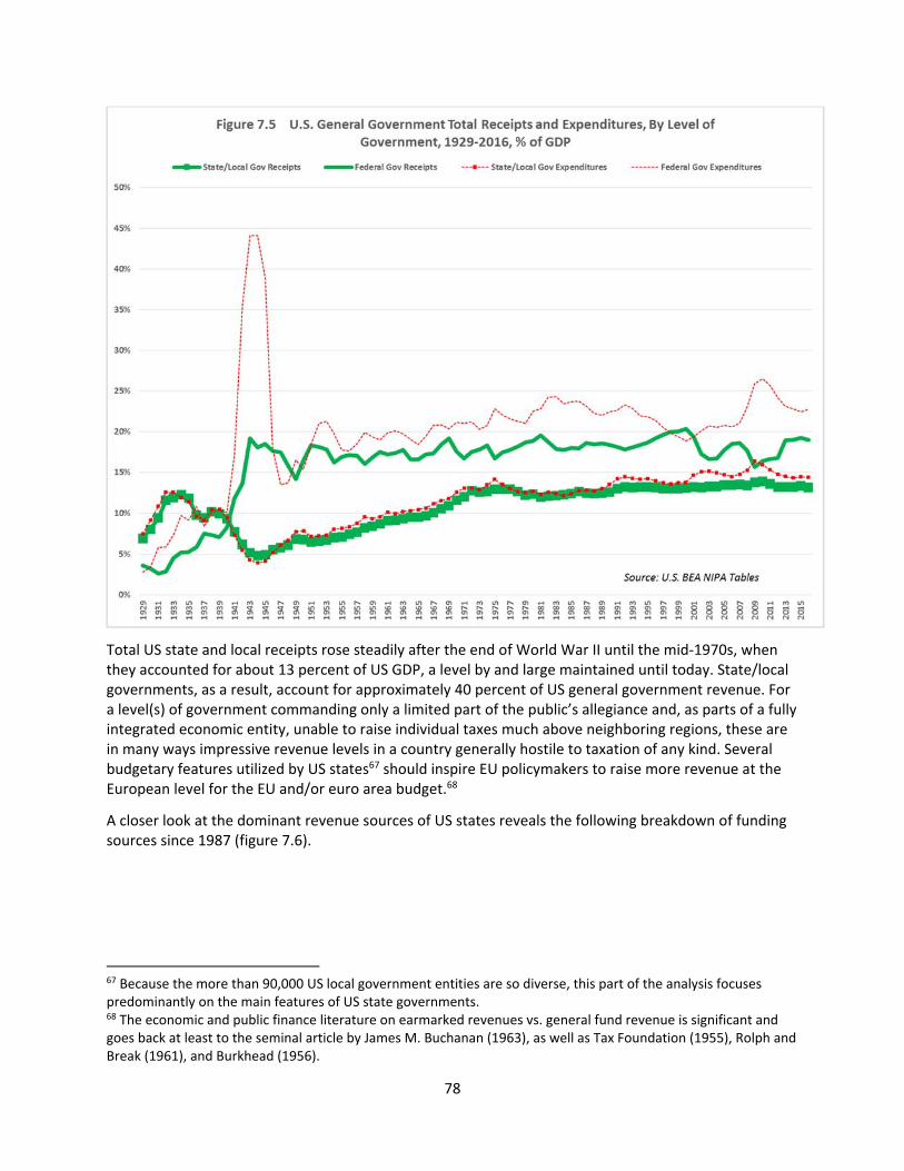
78  

 

Total US state and local receipts rose steadily after the end of World War II until the mid‐1970s, when they accounted for about 13 percent of US GDP, a level by and large maintained until today. State/local governments, as a result, account for approximately 40 percent of US general government revenue. For a level(s) of government commanding only a limited part of the public’s allegiance and, as parts of a fully integrated economic entity, unable to raise individual taxes much above neighboring regions, these are in many ways impressive revenue levels in a country generally hostile to taxation of any kind. Several budgetary features utilized by US states67 should inspire EU policymakers to raise more revenue at the European level for the EU and/or euro area budget.68  

A closer look at the dominant revenue sources of US states reveals the following breakdown of funding sources since 1987 (figure 7.6). 

                                                            67 Because the more than 90,000 US local government entities are so diverse, this part of the analysis focuses predominantly on the main features of US state governments. 68 The economic and public finance literature on earmarked revenues vs. general fund revenue is significant and goes back at least to the seminal article by James M. Buchanan (1963), as well as Tax Foundation (1955), Rolph and Break (1961), and Burkhead (1956). 

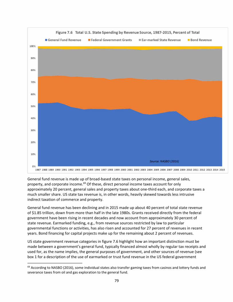
79  

 

General fund revenue is made up of broad‐based state taxes on personal income, general sales, property, and corporate income.69 Of these, direct personal income taxes account for only approximately 20 percent, general sales and property taxes about one‐third each, and corporate taxes a much smaller share. US state tax revenue is, in other words, heavily skewed towards less intrusive indirect taxation of commerce and property. 

General fund revenue has been declining and in 2015 made up about 40 percent of total state revenue of $1.85 trillion, down from more than half in the late 1980s. Grants received directly from the federal government have been rising in recent decades and now account from approximately 30 percent of state revenue. Earmarked funding, e.g., from revenue sources restricted by law to particular governmental functions or activities, has also risen and accounted for 27 percent of revenues in recent years. Bond financing for capital projects make up for the remaining about 2 percent of revenues. 

US state government revenue categories in figure 7.6 highlight how an important distinction must be made between a government’s general fund, typically financed almost wholly by regular tax receipts and used for, as the name implies, the general purposes of government, and other sources of revenue (see box 1 for a description of the use of earmarked or trust fund revenue in the US federal government 

                                                            69 According to NASBO (2016), some individual states also transfer gaming taxes from casinos and lottery funds and severance taxes from oil and gas exploration to the general fund.  

80  

budget.) It is largely up to the sitting state government to spend general fund resources on purposes it sees fit, in correspondence with its sovereign democratic mandate and economic and political priorities.  

This contrasts with the other main revenue categories of US state governments: federal government grants, earmarked state government revenue, and proceeds from bond sales. The federal government grants to state governments invariably come with very limited discretion available for the state government concerning how the proceeds are spent, as grants must be utilized according to often very detailed federal policy prescriptions.70 Similarly, by definition, earmarked or so‐called trust fund revenue71 comes with very limited or no discretion for state governments concerning its use, unless it chooses to change the relevant law(s). This category of state revenues is by law dedicated for specific preidentified purposes and can legally be collected only for such stated purposes. Revenue from state bond sales, which is overwhelmingly for capital investment projects and not for deficit financing purposes, must also be spent according to the bond’s prespecified covenants.  

Figure 7.6 shows that US state governments have a say in the use of only a minority of their budget resources. For sub‐state entities in a federal system, this is an unavoidable effect of state centralization, and in the case of the United States a historical function of the repeated instances where the federal government had to marshal the nation’s entire resources for war fighting purposes.72 Yet for state entities with their own constitutionally enshrined sovereignty, and own regular and competitive democratic mandates, states’ rights will carry less weight when the revenue funding government activities is so heavily restricted. 

At the same time it would be a mistake to regard the lack of budgetary discretion available to US state governments as a restriction on their freedom of action. The direct benefit for state government lawmakers and bureaucrats of having their hands tied on large parts of their budget is that the size of the budget is much bigger, and as a result they administer far larger resources than they otherwise would have been able to do.  

It would be democratically deficient and unacceptable for the US federal government to offer fiscal grants and other economic support to state governments without ensuring that these resources were spent in accordance with politically dictated directions set at the federal level. So unless state governments agree to go along with the federal policy directives—and sometimes in the United States 

                                                            70 State lawmakers, however, probably give as good as they receive in this regard, as their hands might be tied on how to spend the more than $500 billion in annual grants from the federal government. Yet, they themselves get to impose conditions on the almost similarly sized grants from states to local governments ($484 billion in 2014, according to US Census 2015). 71 The US government defines the term “trust fund” differently from private entities. In the standard private common usage, a trust fund is a private fund with a beneficiary that legally owns income streams and most likely also underlying assets. A custodian, or trustee, manages the assets (generating income) on behalf of the beneficiary according to the terms of a preestablished trust agreement guaranteed by a trustor, the only entity that can make changes to the terms of the agreement. In contrast, the US federal or state government is sovereign and owns and manages the assets and income/revenue/earnings of almost all general government trust funds. It can unilaterally change the law to raise or lower future trust fund payments or collections, as well as change the purpose for which trust fund resources are dedicated. See OMB (2016, 381f). 72 The three main historical episodes leading to a lasting increase in fiscal and general government centralization at the federal level in the United States were the US Civil War (1861–65), US participation in World War I (1917–18) and participation in World War II (1941–45). The federal government also expanded substantially during the economic emergency of the Great Depression of the 1930s. Like the European Union, to a considerable degree, the US federal government has also been the result of the crises during US history that it has been called upon to solve. 

81  

they do not and chose not to take the money from Washington73—they will receive no federal resources.  

But perhaps less intuitively, it is also the case that earmarking federal government revenue towards particular trust funds and purposes identified by law makes it easier for state governments to convince resident populations to hand them the resources. It is inherently easier to convince healthily skeptical American taxpayers about the merits of a well drafted, thoroughly analyzed and net benefit positive earmarked tax than to simply get them to hand over the same additional money for state lawmakers to disburse as they see fit in future fiscal years’ budgets. By choosing to earmark so much of their revenue and place it outside their own discretionary powers, state lawmakers are helping grow the size of their own budgets, albeit by agreeing to tie their own hands and to do just things previously decided. 

EU policymakers contemplating how to raise more traditional own resources (TOR)‐like funding for a reformed EU budget could take inspiration from US state budget practices in several ways. With member states being the completely fiscally dominant (actually only) actor in the European Union and already contributing the vast majority of the existing EU budget in the form of direct VAT and GNI‐linked transfers (figure 7.1), there is nothing to gain by trying to implement any additional “US grant‐like funding features” in the EU budget. Indeed, in some ways the existing direct VAT and GNI‐based transfers from member states is preferable to highly regulated US federal government grants, as central “European level” discretion over the EU budget is arguably bigger once member states have signed off on another of the European Union’s seven‐year budget cycles. The focus must instead be on how to replicate the extent of US state (and federal government) reliance on earmarked funding for their budgets. 

Earmarked Revenue Flowing Directly to the EU Budget. European public resistance to pay taxes directly into the EU budget could be overcome by introducing budget mechanisms that earmark such collected revenue for specifically identified policy issues. This would allow for EU budgets to establish “US style trust fund structures” to address specific tasks best solved (e.g., with most European value added) at the regional level.  

Such EU budget trust funds could be directly financed in several ways of increasing potential scale: 

1. Explicit User Fees. Some EU‐level tasks would be explicitly funded through earmarked user fees. A recent example discussed in Kirkegaard (2015b) would be for European external border control measures to be at least partly funded directly by user fees on EU/member state visas for visit, work, study or other activities. This particular type of use fee would moreover have the political advantage of taxing foreigners rather than voters. As analyzed in detail in Kandel (2015), it also has a precedent in the US federal budget, where the US Citizenship and Immigration Services, responsible for issuing visas to the United States, is 95 percent funded by user (e.g., application) fees. Another category of explicit user fees is arrangements according to the “polluter pays principle.” This structure was used in the recently established banking union’s Single Resolution Fund, which will in time be exclusively funded by fees on participating EU banks. 

2. Fees on Related Use Items. Some type of issues, such as financing of EU infrastructure, could, in a manner similar to the US Highway Trust Fund, be financed by small fees on related products 

                                                            73 The highest profile recent case of state governments willingly forgoing sizable available federal government grants is the refusal of 19 US states to take federal government grant resources to fund initially 100 and by 2020 90 percent of the Affordable Care Act (Obamacare) expansion of healthcare coverage to low‐income families through the Medicaid program. See http://familiesusa.org/product/50‐state‐look‐medicaid‐expansion.  

82  

and services like gasoline, air/sea tickets, and natural resource/electricity distribution. Another such option would be for EU renewable energy and smart grid infrastructure to be funded by proceeds from instituting a gradually rising price floor on the European Union’s existing carbon emissions trading system (ETS). An EU‐level fee on various items deemed to be of “inherent danger” to the public, or on all types of insurance policies could also be charged. Proceeds would be channeled into a new EU Disaster Relief Trust Fund that would finance EU relief efforts in response to natural or man‐made disasters across the EU (and around the world). Such an earmarked fund could be used to finance a EU Civil Protection Force along the lines of what French President Emmanuel Macron has recently proposed.74 Such a force would be functionally similar to the US government’s Federal Emergency Management Agency (FEMA).   

3. Broad‐based Taxes Explicitly Earmarked for Particular EU Level Tasks. A potentially far‐reaching budget invention in the European Union would be establishment of budget trust funds funded directly by broad income, payroll, consumption, or other types of taxes. This would be functionally similar to the US federal government’s Social Security Trust Fund(s), which are funded through federal payroll taxes. Such trust funds could be earmarked towards financing large existing or new EU policy areas. 

Assuming new funding structures are agreed in conjunction with adding new policy areas to the EU budget, a gradual shift away from the current funding structure and towards more trust fund budgeting could be envisioned. This would also allow for more EU level initiatives to be initiated without the need to rework the entire existing (and politically set in stone) 7‐year budget agreement. At the same time, provided there is political will, one could also imagine that large existing EU budget expense categories be converted to an earmarked trust fund basis. The funding of EU agricultural support,75 accounting for 40 percent (€58 billion in 2015) of the current EU budget, might be easier to sustain at current funding levels in the future, if it were funded through say an earmarked VAT on food sold in the European Union. 

 

Box 1  Trust Fund Revenue in the US Federal Budget 

Like state budgets, the US federal government budget to a significant degree operates through trust funds, though unlike states the US Treasury general fund is the largest single budget item. The Treasury general fund is also known as the federal funds group in the budget and by definition includes all financial transactions of the federal government not required by law to be conducted through ear‐marked trust funds. The general fund receives all revenue not dedicated to separate budget funds, including essentially all federal income and excise tax revenue. It funds all federal government activities and programs not funded by earmarked trust (or special76 or revolving77) funds.  

                                                            74 See http://international.blogs.ouest‐france.fr/archive/2017/09/29/macron‐sorbonne‐verbatim‐europe‐18583.html  75 This item is termed “Sustainable Growth: Natural Resources” in the current EU budget. 76 Special funds are generally associated with earmarked revenue from government imposition of fines, the sale of government land or assets, or fees for usage of federal government property. Special funds include the Crime Victims Fund, receipts from the sale of timber cut from federal land, and royalties from oil and gas exploration on federal land. Importantly, special fund revenue must be regularly (re)appropriated by Congress before it can be spent on its earmarked purpose. 77 Revolving funds are used to continue business activities involving the ongoing provision of goods and services from federal government assets. In contrast to special funds, proceeds into revolving funds do not require congressional appropriation and are available immediately for their identified expenditure purpose. 

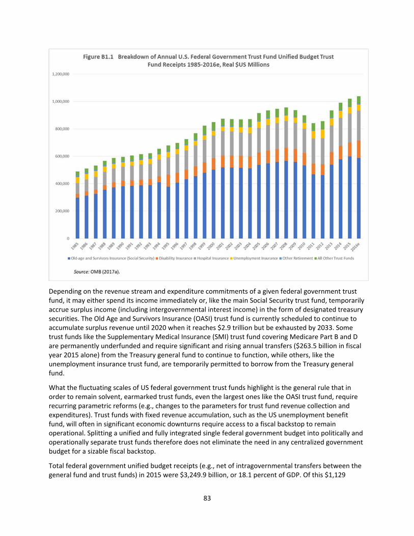
83  

 

Depending on the revenue stream and expenditure commitments of a given federal government trust fund, it may either spend its income immediately or, like the main Social Security trust fund, temporarily accrue surplus income (including intergovernmental interest income) in the form of designated treasury securities. The Old Age and Survivors Insurance (OASI) trust fund is currently scheduled to continue to accumulate surplus revenue until 2020 when it reaches $2.9 trillion but be exhausted by 2033. Some trust funds like the Supplementary Medical Insurance (SMI) trust fund covering Medicare Part B and D are permanently underfunded and require significant and rising annual transfers ($263.5 billion in fiscal year 2015 alone) from the Treasury general fund to continue to function, while others, like the unemployment insurance trust fund, are temporarily permitted to borrow from the Treasury general fund. 

What the fluctuating scales of US federal government trust funds highlight is the general rule that in order to remain solvent, earmarked trust funds, even the largest ones like the OASI trust fund, require recurring parametric reforms (e.g., changes to the parameters for trust fund revenue collection and expenditures). Trust funds with fixed revenue accumulation, such as the US unemployment benefit fund, will often in significant economic downturns require access to a fiscal backstop to remain operational. Splitting a unified and fully integrated single federal government budget into politically and operationally separate trust funds therefore does not eliminate the need in any centralized government budget for a sizable fiscal backstop.  

Total federal government unified budget receipts (e.g., net of intragovernmental transfers between the general fund and trust funds) in 2015 were $3,249.9 billion, or 18.1 percent of GDP. Of this $1,129 

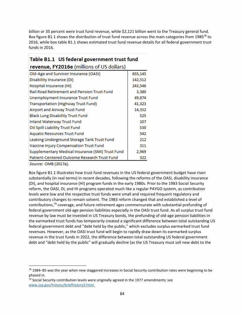
84  

billion or 35 percent were trust fund revenue, while $2,121 billion went to the Treasury general fund. Box figure B1.1 shows the distribution of trust fund revenue across the main categories from 198578 to 2016, while box table B1.1 shows estimated trust fund revenue details for all federal government trust funds in 2016. 

 

Box figure B1.1 illustrates how trust fund revenues in the US federal government budget have risen substantially (in real terms) in recent decades, following the reforms of the OASI, disability insurance (DI), and hospital insurance (HI) program funds in the early 1980s. Prior to the 1983 Social Security reform, the OASI, DI, and HI programs operated much like a regular PAYGO system, as contribution levels were low and the respective trust funds were small and required frequent regulatory and contributory changes to remain solvent. The 1983 reform changed that and established a level of contributions,79 coverage, and future retirement ages commensurate with substantial prefunding of federal government old‐age pension liabilities especially in the OASI trust fund. As all surplus trust fund revenue by law must be invested in US Treasury bonds, the prefunding of old‐age pension liabilities in the earmarked trust funds has temporarily created a significant difference between total outstanding US federal government debt and “debt held by the public,” which excludes surplus earmarked trust fund revenues. However, as the OASI trust fund will begin to rapidly draw down its earmarked surplus revenue in the trust funds in 2022, the difference between total outstanding US federal government debt and “debt held by the public” will gradually decline (as the US Treasury must sell new debt to the 

                                                            78 1984–85 was the year when new staggered increases in Social Security contribution rates were beginning to be phased in. 79 Social Security contribution levels were originally agreed in the 1977 amendments; see www.ssa.gov/history/briefhistory3.html.  

85  

public to redeem the bonds held by the trust fund when it pays out benefits) with the predicted exhaustion of the OASI trust fund by 2033 under current law.80 

Box table B1.1, while again highlighting the dominant size of the OASI and other social insurance trust funds in the federal government budget, also makes it clear how the earmarked revenue trust fund model is used in a variety of different policy areas in the federal budget. Sea, land and air infrastructure, environmental concerns, disease and medical research are all subject areas funded by US federal government trust fund structure. This illustrates the versatility of the funding model and how it could be utilized in many different ways to also finance parts of a future EU budget. 

End box. 

 

8 The Federal Highway Trust Fund81 

The US federal government Highway Trust Fund (HTF) was set up by President Dwight Eisenhower in 1956 to fund federal government investments to expand the US interstate highways82 Since the interstate highway system, as the name implies, connects America’s states (at least the 48 states in continental America, not counting Alaska and Hawaii) and was—at the time—viewed as having important national security implications, this was viewed as a natural task for the federal government. The HTF also has a smaller separate account (approximately 13 percent of total HTF revenue) for financing urban mass transit projects, though the majority of spending goes towards traditional highways.  

Public spending accounts for the vast majority of total US infrastructure spending going towards highways and mass transit systems, with public‐private partnerships accounting for less than 1 percent of the cumulative total for the last 25 years (CBO 2015b). State and local governments account for the majority—almost three‐quarters—of total public spending, as these entities are responsible for operations and maintenance of both highways and urban mass transits. Federal government spending, in contrast, goes overwhelmingly towards capital investments, e.g., building new and improving existing highways.83 Total new capital investments in highways and mass transit is split roughly 50‐50 between states and the federal government, with spending levels in 2014 at $44 billion and $48 billion respectively. Inflation‐adjusted total public spending towards highways and mass transit systems has declined in the last decade and in 2014 stood at $118 billion and $46 billion for state and local governments and the federal government, respectively. 

The HTF is financed through several earmarked federal fuel (excise) taxes on gasoline and diesel fuels sold throughout the United States, as well as taxes on heavy trucks and trailers, certain other heavy 

                                                            80 It is frequently asserted that Social Security goes bankrupt when the trust fund is exhausted. This is somewhat misleading, because—if there is no reform of any kind—Social Security merely reverts to a standard earmarked PAYGO system, which can pay out only the amounts in benefits that it collects in contributions. This is estimated to lead to an approximately 22 percent immediate reduction in Social Security benefits after 2033. Politically and economically, the main beneficiaries of such a “no reform scenario” will be American retirees who die shortly before the exhaustion of the trust funds, as they will bear none of the costs of restoring the Social Security program to balance. 81 This section updates and expands the discussion in Kirkegaard (2015a, 25). 82 Previously, federal road construction in the United States had been funded directly from the US Treasury general funds.  83 Federal government operations and maintenance expenditure ($3 billion in 2014) are related to infrastructure in the District of Columbia and on federally owned land. 

86  

vehicles, and truck tires. Gasoline taxes have since 1993 been set at 18.4 cents/gallon84 sold and account for 62 percent of total HTF revenue, diesel fuel taxes of 24.4 cents/gallon account for 25 percent of HTF revenue, trucks and trailer taxes for 10 percent, while other vehicle and tire taxes for the remaining approximately 3 percent of HTF revenue. 

The current level of the fuel taxes has been left unchanged by Congress since 1993. This has left the HTF underfinanced due to inflation and legislated rising fuel efficiencies in the American car park The HTF therefore needs occasional congressionally approved budget support from regular federal government funds to continue to finance required new US road infrastructure and maintenance work. These transfers of revenue from the Treasury general fund have been substantial in recent years due to accelerating underfunding, amounting to $143 billion from 2008 to the present (CBO 2016). In 2016 Congress passed a new 5‐year spending bill for the HTF, intended to balance trust fund revenue and outlays with approximately $70 billion in new transfers from the general fund until 2021 (Kirk and Mallett 2016). Current CBO projections, however, suggest a further cumulative HTF underfunding of $139 billion from 2021 to 2027, as Congress has not brought earmarked revenues in line with expected outlays.  

For instance, unlike the federal unemployment trust fund, which as a cyclically sensitive fund is expected to occasionally go into potential temporary deficits (from temporary increases in unemployment benefit payments) and hence has the ability to explicitly borrow from the Treasury general fund, the HTF funds only long‐term capital infrastructure projects. Such federally funded infrastructure in the United States, being paid for by earmarked taxes, does not generate user fee income. The HTF therefore has no way to recoup any revenue shortfalls from future revenue streams, as Congress remains unwilling to raise earmarked fuel (and other) taxes. Taking out loans from the federal government hence makes little sense, as earlier years’ revenue shortfalls will not be made up in the future unless new investments are reduced. Congress, no doubt affected by the general popularity of new federal government infrastructure spending, hence prefers to simply transfer general fund revenue towards this popular spending item, rather than adjust earmarked fuel and other tax revenues to balance the HTF’s revenue and expenditure. As long as raising fuel taxes remains a highly unpopular measure and overall federal government budget consolidation is not pursued, the HTF is likely to remain structurally underfunded and in need of congressional authorization of regular transfers of general fund resources. 

While the HTF is under financial stress, it has successfully for decades represented a form of implicit federal‐level American road‐pricing, as it is America’s drivers (and especially drivers of heavy vehicles) who through their fuel purchases finance the construction and improvements of the inter‐state highways on which they drive.  

States vary greatly in their financing and budget treatment of their (larger) highway and mass transit infrastructure investments and maintenance costs. Some rely on earmarked funding from state fuel taxes similar to that of the federal government, while others simply fund these items from regular general fund revenue. There is no specific limit to state financing of infrastructure eligible for federal cofinancing (includes both interstate highways and other roads in the National Highway System85), but historically the split for new capital investments has been 50‐50, while states are also responsible for maintenance. Due to cyclicality of general state revenue and also fuel tax revenue (Americans generally 

                                                            84 18.3 cents/gallon goes towards the HTF, while 0.1 cent/gallon is transferred towards the environmental clean‐up fund, the Leaking Underground Storage Tank Trust Fund. 85 The National Highway System includes all interstate highways, as well as other roads serving major population centers, border crossings, transportation facilities (mass transit), and important travel destinations in the form of major cities, beaches, or national parks. 

87  

drive less during recessions), prolonged recessions as in 2007–09 tends to put state cofinancing of long‐term multiyear highway infrastructure projects at risk. As a result, the federal government, with its superior ability for debt financing, tends to include higher cofinancing of infrastructure projects as part of federal government economic stimulus bills. There is not, however, a general intent in the HTF or the general federal government budget to prioritize infrastructure spending in periods of economic downturns.86 Rather the explicit policy intent of the HTF is to provide transparent and predictable long‐term earmarked financing of infrastructure in the United States.  

9 Scope and Function of US States’ Budget Stabilizers and Rainy Day Funds  

US states are generally subject to various budgetary restrictions aiming to push them towards running a balanced budget and limiting debt issuance. Their sources of revenue are often cyclically more volatile, too, and as a result their services provision is vulnerable to economic downturns and unanticipated manmade or natural disasters. As a result, US states as a rule run sizable cash balances (e.g., cash surpluses at the end of a fiscal year) and often maintain dedicated rainy day funds to ensure uninterrupted services provision to state residents.  

Rainy day funds account for the largest share of states’ total balances. These funds are explicitly designed and created to mitigate disruptions to states’ services provision during an economic downturn. They are also the means for states to respond to unforeseen circumstances during a fiscal year: Specific “disaster response funds” are earmarked to help states address unforeseen manmade and natural disasters during a fiscal year. 

In several states, total rainy day funds are, moreover, split into several funds earmarked towards safeguarding particular state government functions. The bulk of funds are dedicated to general budget stabilization, but special directed rainy day funds are focused on general education and tuition assistance and state Medicaid expenses (e.g., healthcare provision for the poorest residents).87 

States’ total balances (and rainy day funds) naturally vary considerably over the national economic cycle, as individual states may be affected by asymmetric economic shocks or local economic booms. Figure 9.1 shows the trends in states’ total balances from 1979 to 2017(p). 

                                                            86 The proposed Grant Act from 1932 suggested such a cyclically sensitive approach towards federal infrastructure spending but was not adopted by Congress. 87 NASBO (2015, table 14) presents a detailed look at each state’s legal rainy day framework. 

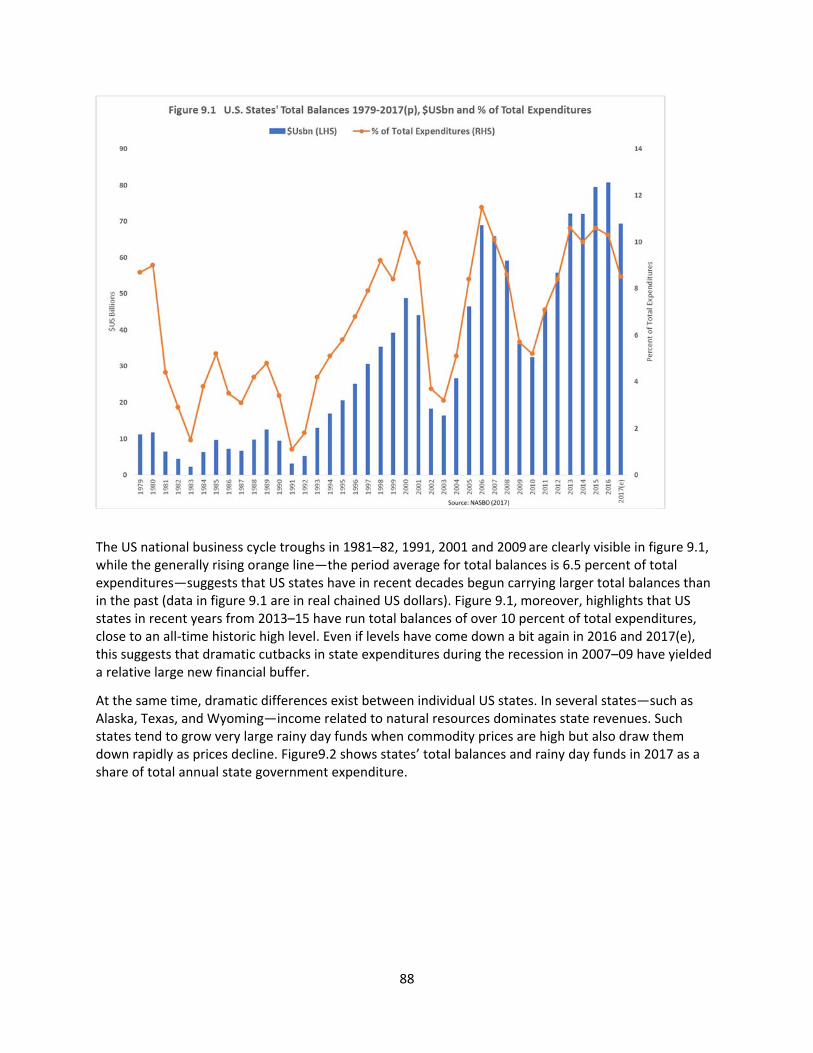
88  

  

The US national business cycle troughs in 1981–82, 1991, 2001 and 2009 are clearly visible in figure 9.1, while the generally rising orange line—the period average for total balances is 6.5 percent of total expenditures—suggests that US states have in recent decades begun carrying larger total balances than in the past (data in figure 9.1 are in real chained US dollars). Figure 9.1, moreover, highlights that US states in recent years from 2013–15 have run total balances of over 10 percent of total expenditures, close to an all‐time historic high level. Even if levels have come down a bit again in 2016 and 2017(e), this suggests that dramatic cutbacks in state expenditures during the recession in 2007–09 have yielded a relative large new financial buffer. 

At the same time, dramatic differences exist between individual US states. In several states—such as Alaska, Texas, and Wyoming—income related to natural resources dominates state revenues. Such states tend to grow very large rainy day funds when commodity prices are high but also draw them down rapidly as prices decline. Figure9.2 shows states’ total balances and rainy day funds in 2017 as a share of total annual state government expenditure.  

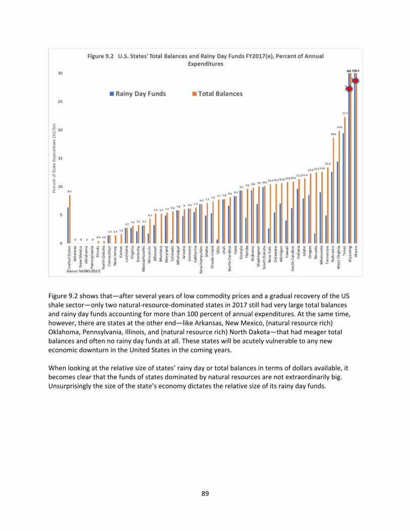
89  

 

 Figure 9.2 shows that—after several years of low commodity prices and a gradual recovery of the US shale sector—only two natural‐resource‐dominated states in 2017 still had very large total balances and rainy day funds accounting for more than 100 percent of annual expenditures. At the same time, however, there are states at the other end—like Arkansas, New Mexico, (natural resource rich) Oklahoma, Pennsylvania, Illinois, and (natural resource rich) North Dakota—that had meager total balances and often no rainy day funds at all. These states will be acutely vulnerable to any new economic downturn in the United States in the coming years.  

When looking at the relative size of states’ rainy day or total balances in terms of dollars available, it becomes clear that the funds of states dominated by natural resources are not extraordinarily big. Unsurprisingly the size of the state’s economy dictates the relative size of its rainy day funds. 

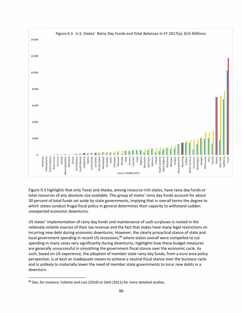
90  

  

 Figure 9.3 highlights that only Texas and Alaska, among resource‐rich states, have rainy day funds or total resources of any absolute size available. This group of states’ rainy day funds account for about 30 percent of total funds set aside by state governments, implying that in overall terms the degree to which states conduct frugal fiscal policy in general determines their capacity to withstand sudden unexpected economic downturns.  US states’ implementation of rainy day funds and maintenance of cash surpluses is rooted in the relatively volatile sources of their tax revenue and the fact that states have many legal restrictions on incurring new debt during economic downturns. However, the clearly procyclical stance of state and local government spending in recent US recessions,88 where states overall were compelled to cut spending in many cases very significantly during downturns, highlights how these budget measures are generally unsuccessful in smoothing the government fiscal stance over the economic cycle. As such, based on US experience, the adoption of member state rainy day funds, from a euro area policy perspective, is at best an inadequate means to achieve a neutral fiscal stance over the business cycle and is unlikely to materially lower the need of member state governments to incur new debts in a downturn. 

                                                            88 See, for instance, Follette and Lutz (2010) or GAO (2011) for more detailed studies. 

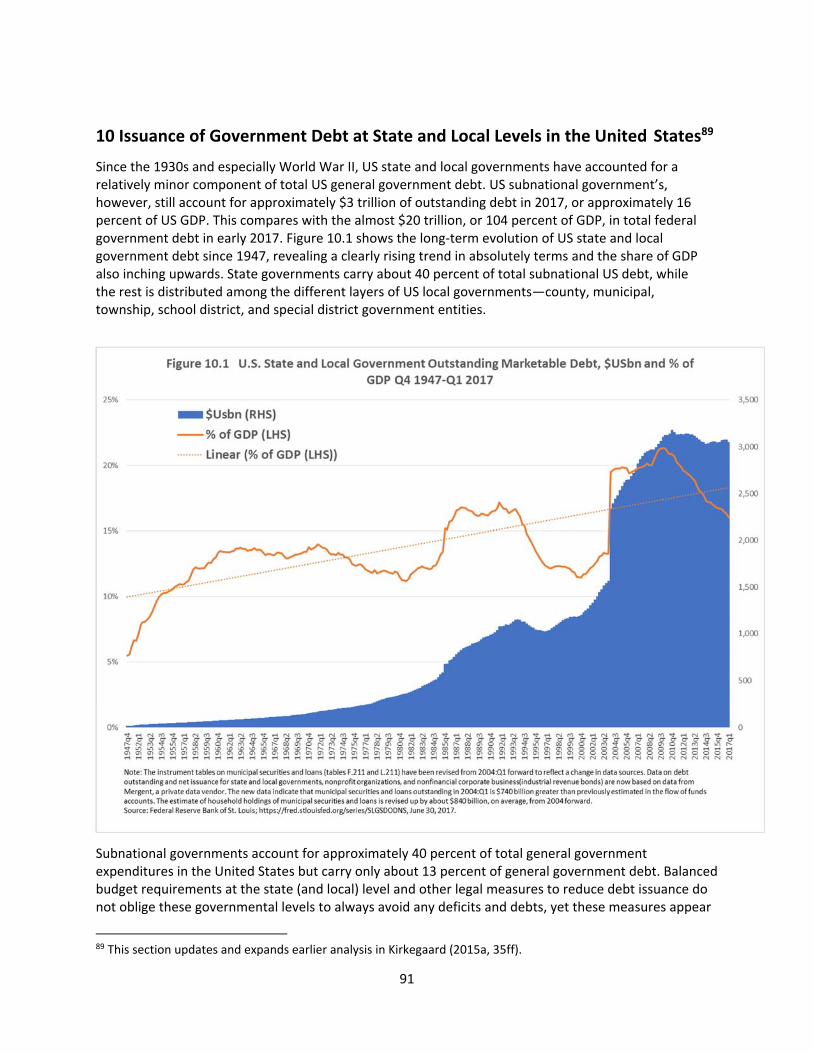
91  

 

10 Issuance of Government Debt at State and Local Levels in the United  States89 

Since the 1930s and especially World War II, US state and local governments have accounted for a relatively minor component of total US general government debt. US subnational government’s, however, still account for approximately $3 trillion of outstanding debt in 2017, or approximately 16 percent of US GDP. This compares with the almost $20 trillion, or 104 percent of GDP, in total federal government debt in early 2017. Figure 10.1 shows the long‐term evolution of US state and local government debt since 1947, revealing a clearly rising trend in absolutely terms and the share of GDP also inching upwards. State governments carry about 40 percent of total subnational US debt, while the rest is distributed among the different layers of US local governments—county, municipal, township, school district, and special district government entities.  

 

Subnational governments account for approximately 40 percent of total general government expenditures in the United States but carry only about 13 percent of general government debt. Balanced budget requirements at the state (and local) level and other legal measures to reduce debt issuance do not oblige these governmental levels to always avoid any deficits and debts, yet these measures appear 

                                                            89 This section updates and expands earlier analysis in Kirkegaard (2015a, 35ff). 

92  

to have ensured that the main government debt burden in the United States is carried at the federal government level. 

The large number of different local government bond issuers in the United States provides for substantial variation among marketable debt issued by individual US state and local government entities. These range from large US states like California, which if it were an independent state would be a member of the G‐7, to the smallest rural township and school districts in the interior of the country. The state and local government bond market, also known as the municipal bond market (or “munis” for short), consists of debt securities issued to fund day‐to‐day obligations and to finance capital projects such as building schools, highways, and sewer systems. 

Crucially, to secure a stable investor base for highly diverse municipal bonds, the federal government exempts the interest income from these bonds from federal income taxes. This tax benefit to state and local government bonds cost the federal government approximately $30 billion in forgone tax revenue in 2017,90 and is estimated to rise to $50 billion by 2024. This is a sizable implicit financial transfer from the US federal government to state and local governments and has several important implications for the state and local government bond market.  

First, it means that the after‐tax interest income available to investors on state and local government bonds is highly attractive, providing state and local governments with powerful market support for placing their debts in competition with other saving products. 

Second, while some state and local governments also exempt interest income accruing to locally resident holders on their own bonds from local taxation, the fact that federal income tax rates far exceed such local taxes creates a powerful tool for the creation of a large and liquid national US market for this category of debt. 

Third, wealthy individual US‐based investors eager to escape higher personal federal income tax rates have a strong preference for purchasing generally safe and highly rated state and local government bonds. Ownership of this category of debt is extremely low among financial institutions,91 because the individual tax exemptions do not apply to corporate income. For instance, banks own next to no state and local government debt. Instead, the typical investor is a wealthy elderly American individual seeking a stable stream of tax‐exempt payments in retirement. 

Fourth, this tax‐exempt status of state and local government debt means that establishing public‐private partnerships (PPPs) to finance large infrastructure projects and other investments in the United States is almost always a financially suboptimal solution for investors, when compared with straightforward financing by a state and/or local government entity. For instance, in highway construction, where PPPs for toll roads are common in many European countries, such PPPs in the United States have accounted for less than 1 percent of all investments in recent decades (CBO 2015b). This is ironic because the United States is considered more market‐oriented, but due to federal tax laws the benefits of private sector involvement in terms of better and more timely project execution pale in comparison to the financing benefits of state and local government debt issuance.  

The two main types of municipal bonds in existence are:92 

                                                            90 See OMB (2017c, table 13.1). 91 Many financial firms offer bond funds consisting of state and local government bonds to their clients, but they do not carry this debt on their own balance sheets. 92 In addition, municipal borrowers sometimes issue bonds on behalf of private entities such as nonprofit colleges or hospitals. These “conduit” borrowers typically agree to repay the issuer, who pays the interest and principal on 

93  

General obligation bonds: issued by states, cities, counties, or other governmental entities with direct taxing powers and not secured by any assets. Instead, general obligation bonds are backed by the “full faith and credit” of the issuer, which has the power to tax residents to pay bondholders. It varies from issuer to issuer whether bondholders’ claims on tax proceeds have legal priority over financial claims on the government from other stakeholders. 

Revenue bonds: issued by states, cities, counties, or other governmental entities with or without direct taxing powers and not backed by government’s taxing power, but instead by revenues from a specific project or source, such as highway tolls or lease fees. Some revenue bonds are “nonrecourse,” meaning that if the revenue stream dries up, the bondholders do not have a claim on the underlying revenue source. 

The diversity of state and local government issuers means important legal distinctions matter for the overall munis market. As US states are legally sovereign entities, they cannot declare bankruptcy under US federal law, as this would by definition violate their sovereign status under the US Constitution.  

Unlike US local governments, which as legal corporations may under some circumstances file for federal bankruptcy protection (see below), state governments possess sovereign and, in principle, constitutionally uninhibited taxing powers.93 During economic crises and associated difficulties in making bond payments, US states must reach a negotiated settlement with their creditors to retain access to financial markets. This is a predictably tortuous political process, as bondholders invariably demand that states raise taxes to repay their debts—which in the case of “general obligation bonds” are backed by the full faith and credit of the state government. Only one US state has since the 1840s chosen to go down this route, namely Arkansas at the height of the Great Depression in 1933.94 In this historical case, only a commitment by the Arkansas government to raise the state’s automobile and gasoline taxes and earmark all proceeds to highway maintenance and debt service eventually won over its creditors, enabling it to return to a state of normal public debt service provision and governmental function. 

The situation is very different for US local governmental entities, as they can seek protection from their creditors in US federal bankruptcy court under Chapter 9 of the US federal bankruptcy code. With about $1.8 trillion in outstanding US local government debt (roughly 60 percent of the total in figure 10.1), this means that just over 10 percent of all US general government debt held by the public is in theory subject to debt restructuring through a formal federal bankruptcy procedure. However, due to state‐level restrictions on the ability of in‐state local government entities to declare bankruptcy, in reality the total amount of US general government debt subject to restructuring is somewhat lower. 

Availability of Chapter 9 bankruptcy procedures is further subject to some legal conditionality. 

                                                            the bonds. In cases where the conduit borrower fails to make a payment, the issuer usually is not required to pay the bondholders. 93 It is important to note, however, that in reality in a closely integrated national economy like the United States, there are relatively low limits for how far individual states can diverge in terms of taxation from its neighboring states without creating potentially significant “border effects” and risk losing economic activity. 94 For details of the Arkansas default, see Mysak (2010). California’s well‐published reliance on IOUs (I Owe You) to pay some budget items (like state tax refunds) in 2009 was ultimately determined to be a legal default. The delay was temporary (only a few months), and all IOUs were redeemed by the state government, plus interest, and did de facto function as a temporary cash equivalent in California with most large banks accepting them as regular payments. Consequently, the Californian IOUs consistently traded very close to their par value and no private holder took the state to court—a legal task anyway greatly complicated by the sovereign status of the state of California. 

94  

Bankruptcy under federal law and Chapter 9 is conditional and subject to four legal criteria (CBO 2010): 

 1. The entity must be a political subdivision, public agency, or instrumentality of a state. Ipso 

facto, states themselves are not allowed to file. 2. State law must authorize that its governmental entities rely on Chapter 9 and federal 

bankruptcy law. This is a major restriction, as only 26 US states allow their local government entities to file under Chapter 9, and of these 14 demand that a local government seek the explicit consent of a state authority before proceeding. Georgia outright prohibits its local government entities from filing under Chapter 9, while the remaining 23 states have no laws addressing this issue. That though means that municipalities here would only be able to file under Chapter 9 if a new state law explicitly permitted them to. Or in other words, seek the approval not only of a state executive officer but also from a majority of the legislative branch through the passing of new state law. 

3. The filing local government entity must be insolvent. 4. The local government entity must first, to the extent practical, negotiate in good faith with its 

creditors to restructure its debts outside bankruptcy, which can therefore only be an ultima ratio option for any local government entity. 

It is clear from these four criteria that a degree of political and legal discretion exists when determining whether a local government bankruptcy is possible under Chapter 9. Bondholders will seek to block bankruptcy filings to get all their money back, making for instance what constitutes an entity’s prior “good faith negotiations” with creditors almost invariably the subject of separate and often lengthy legal battles. This is to discern whether a particular bankruptcy petition is admissible in the federal court system and Chapter 9.  

Recently, following the debt crisis in Puerto Rico, a US dependent territory, where residents are US citizens but it is itself not a sovereign US state, an important expansion of bankruptcy options for some US general government debt was established. In 2016 Congress passed the Puerto Rico Oversight, Management, and Economic Stability Act, or PROMESA Law. Functionally similar to an International Monetary Fund (IMF) program, the law establishes a fiscal oversight board tasked with reforming Puerto Rican government finances and provides for a Chapter 9–like process for the restructuring of Puerto Rican debt, including crucially protection for the Puerto Rican government from creditor‐initiated litigation. As a result of PROMESA, the debts of all dependent US territories, including the US Virgin Islands, American Samoa, Guam, or the Northern Mariana Islands, are now de facto subject to Chapter 9–like processes.  

Given how the US municipal bond market is integrated across the entire United States, local in‐state ownership of US local government debt is not high, despite attempts by some state governments to lure their domestic in‐state investors towards their bonds by exempting interests also from state income tax. Rather this debt is widely distributed across investors geographically located throughout the United States. This has the political implication that there is generally no compelling bond market reason for state governments to come to the financial rescue of any defaulting local governmental entities in the state, as local in‐state bond investors will generally not suffer particular concentrated financial losses. There may of course be other good reasons of reputation and short‐term political concerns for a state government to offer assistance to a local governmental entity in financial trouble. 

Market discipline, in the form of rising interest rates for more indebted states and local government 

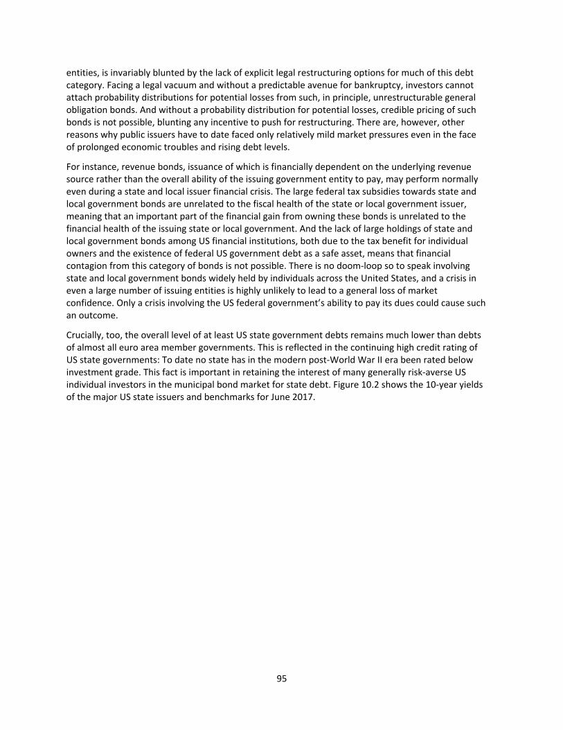
95  

entities, is invariably blunted by the lack of explicit legal restructuring options for much of this debt category. Facing a legal vacuum and without a predictable avenue for bankruptcy, investors cannot attach probability distributions for potential losses from such, in principle, unrestructurable general obligation bonds. And without a probability distribution for potential losses, credible pricing of such bonds is not possible, blunting any incentive to push for restructuring. There are, however, other reasons why public issuers have to date faced only relatively mild market pressures even in the face of prolonged economic troubles and rising debt levels.  

For instance, revenue bonds, issuance of which is financially dependent on the underlying revenue source rather than the overall ability of the issuing government entity to pay, may perform normally even during a state and local issuer financial crisis. The large federal tax subsidies towards state and local government bonds are unrelated to the fiscal health of the state or local government issuer, meaning that an important part of the financial gain from owning these bonds is unrelated to the financial health of the issuing state or local government. And the lack of large holdings of state and local government bonds among US financial institutions, both due to the tax benefit for individual owners and the existence of federal US government debt as a safe asset, means that financial contagion from this category of bonds is not possible. There is no doom‐loop so to speak involving state and local government bonds widely held by individuals across the United States, and a crisis in even a large number of issuing entities is highly unlikely to lead to a general loss of market confidence. Only a crisis involving the US federal government’s ability to pay its dues could cause such an outcome. 

Crucially, too, the overall level of at least US state government debts remains much lower than debts of almost all euro area member governments. This is reflected in the continuing high credit rating of US state governments: To date no state has in the modern post‐World War II era been rated below investment grade. This fact is important in retaining the interest of many generally risk‐averse US individual investors in the municipal bond market for state debt. Figure 10.2 shows the 10‐year yields of the major US state issuers and benchmarks for June 2017. 

96  

 

 

Figure 10.2 makes it clear that several US states enjoy yields lower than the US federal government benchmark, which is unsurprising in light of their solid AAA ratings. However, at the other end of the rating spectrum, it can be seen that Illinois just above junk rating at BBB– and New Jersey at A– do face a market risk premia of about 250 basis points and over 100 basis points, respectively, relative to the federal government debt. This is a significant market penalty but given the continuous budget crisis these two states have been in in recent years still a modest one, especially in comparison to the risk premia witnessed for some euro area members in the years after 2010. 

At the same time, however, local government entities with severely impaired finances are likely to be shut out of financial markets completely, skewing the level of market discipline operating in the US municipal bond market—after all, loss of market access is the most severe discipline of all. This issue matters a great deal more among the tens of thousands of highly diverse local government entities in the United States, as some are frequently discouraged from or denied access to debt markets without major spillovers or disruptions. The only real world impact of such an event is that a local infrastructure project might not be built, a school system has to reduce services more than expected, or local government expenditures cut more than otherwise intended. This impact evidently pales compared with the loss of market access for one of the 19 sovereign issuers in the euro area. 

Overall US state and local government debt issuance suggests several lessons for the euro area. First, the market highlights the power and importance of tax incentives in creating a liquid market that is appealing to retail investors (a practice several euro area member states have also long employed). Second, the fact that state and local government debt is not generally used in the financial sector as a safe asset means that at least these bonds can be subject to credit risk without creating market turmoil. Market discipline on US state and local government issuers is hence often muted, especially 

97  

at the state level. These US experiences highlight that restructuring mechanisms for sovereign bonds should be attempted only if another safe asset has been created. In such a scenario, US financial history suggests that the explicit ability to restructure government debt at lower levels of government does not create unmanageable financial market risks for the relevant government issuers.  

11 US States’ Balanced Budget Provisions: Less Stringent Than Often Assumed 

Since the mid‐19th century US state and local governments have been subject to so‐called balanced budget requirements, so the fact that in 2014 US state and local government debts were approximately $3 trillion and interest expenses exceeded $100 billion would, at first glance, appear surprising. The reason for persistent US state and local government indebtedness, however, lies in the complexity of determining what constitutes balanced budget requirements. 

Given the diversity at US local government entities, a comprehensive analysis of their balanced budget requirements is difficult. However, as many local government entities are special purpose constructs, such as school districts, without direct independent taxing powers and able to raise fee income or issue debt only after obtaining explicit permission from higher levels of government, they are subject to de facto budgetary controls and must run balanced budgets. 

Only general purpose local governments, such as counties and municipalities, are able to issue debt, though the degree to which they are restricted in doing so varies greatly from state to state. Often states with very large metropolitan areas, such as New York City in New York state or Chicago in Illinois, have relatively fewer restrictions on the behavior of such large general purpose local governments. Legal balanced budget requirements are, therefore, not the most important force instilling sustainable finances on local governments in the United States. Instead, it is a combination of the legal inability to issue debt and a budgetary structure requiring that expenditure match revenue and then the market discipline that comes from being actually denied new financing, and in some local government entities’ cases, the risk of facing bankruptcy procedures under federal law.  

At the US state level, substantial variations exist in what constitutes a balanced budget, and different academic and official sources have compiled different analytical results for a number of states and conceptual rigidity of states’ balanced budget requirements.95 All agree that almost all US states have some sort of either constitutional or statutory budget restrictions in place. Several issues, though, affect their scope and effectiveness. 

The first issue concerns the budgetary scope of balanced budget requirements. From state lawmakers’ perspective, the legal requirement for a balanced budget typically concerns the need to balance only the operating budget, e.g., the state general fund. States’ general funds are made up of the majority of state general tax revenue and pay out a sizable share of state expenditures. NASBO (2015), though, estimates that in fiscal year 2014 only 41 percent of total state government expenditures came from general funds, while 30 percent came from federal government grants, 27 percent from earmarked revenue sources (such as fuel taxes funding highway investments), and 2 percent from new bond sales. In other words, less than half of states’ spending in 2014 would have been subject to their balanced budget requirements. State lawmakers, thus, have opportunities to legally run deficits in spending vehicles outside the general fund, which are not subject to the constitutional or statutory balanced budget requirements. Yet, at the same time, other implicit budget control functions exist. For instance the 30 percent of state expenditures coming from federal government grants are revenues straight 

                                                            95 Several compilations exist from the GAO (1993), Yilen and Smith (2006), NCSL (2010), and NASBO (2015). 

98  

forward to balance, as states can only allocate as much spending from them as the resources they receive. Other parts of nongeneral fund outlays from within the state are from the 27 percent of earmarked revenues legally required to go towards particular spending priorities, which may not be topped up with other budget resources. As a result, state lawmakers cannot spend additional resources on such expenditure items. 

The main exception for state balanced budget requirements is bond finance for capital projects, with borrowing to be financed explicitly against the future proceeds from the project in question. More generally, it can therefore be argued that US state governments’ capital spending is outside balanced budget rule procedures, and many of the states’ balanced budget rules hence approach so‐called golden rules, where only investments may be debt financed. At the same time though, it should be recalled that such bond‐financed investments account for only a small share—2 percent in 2014—of total state expenditures. 

The second conceptual issue affecting states’ budget restrictions relates to the particular budget procedures required to be in balance. NASBO (2015) reports that in 44 states the governor is required to submit a balanced budget, but only in 41 states is the legislature required to enact a balanced budget and in only 40 states must the budget signed by the governor be in balance. In all three instances, unexpected and unbudgeted events during the fiscal year may occur and cause an actual deficit to occur at the end of the fiscal year, even when the budget was legally “in balance” at the start of the fiscal year. Eleven states have provisions that allow for such unexpected deficits to be carried over into the next year and are therefore not obliged to make up for unexpected spending before the end of the fiscal year. Some states have tougher requirements and explicitly demand that expenditures in a fiscal year are within the cash collected for the same fiscal year. Others, like the Oklahoma constitution, require fiscal year expenditures from the general fund to be automatically reduced dollar‐for‐dollar if projected revenues fall below what is forecast in the budget. Still others like Virginia are weaker, with just a constitutional requirement for the governor to maintain spending on par with revenues, but no mechanism of enforcement. Constitutional provisions elsewhere, as in Michigan, permit so‐called unavoidable deficits to be carried into the next fiscal year, but “unavoidable” is never properly defined, thus opening a pathway for persistent “unavoidable deficit spending.” 

States may also maintain explicit limits to total outstanding authorized debt (40 states) and/or have policies in place that limit resources devoted to debt service (28 states). Targeted tax and expenditure limitations (often ballot initiated by grassroots movements) may also restrict the levels and/or growth rates of state revenues and taxes, typically linked to growth in state personal incomes, population, or inflation. 

The third conceptual issue concerns the substantial expenditure items that generally fall outside government accounting practices. As in the European Union and under the ESA2010, such items include unfunded defined benefit pension and healthcare liabilities for state and local government employees. Depending on the precise discount rate and risk assumptions made, US states’ unfunded pension liabilities alone account for $1 trillion to $3 trillion,96 though with a very large degree of variation among the states.  

Pew (2016), meanwhile, estimates that US states’ so‐called other postretirement employment benefits (OPEBs)—made up overwhelmingly of healthcare costs—accounted for over $620 billion in 2014 and was only 6 percent funded. Since state governments are sovereign, it may be debated whether such unfunded future government liabilities are actual legal commitments or amount merely 

                                                            96 See Gale and Krupkin (2016). 

99  

to “political promises” that policymakers may renege on at any moment. Whatever the correct description is, however, does not change the fact that the ability to exclude or at least obscure these very large current and especially future expenditure items from the regular state budget process has made superficial adherence to balanced budget requirements much easier in the past. 

Yet at the same time, though, in many states a lack of explicit and actually binding balanced budget legal language is counterbalanced by a longstanding historical practice of maintaining (close to) a balanced budget (English 1996). This is backed by the muted degree of market pressure arising from the lack of federal government bailouts of states in the United States since the early 18th century. As such, while almost all US states have some sort of formal legal balanced budget requirements, what is explicitly meant is often subject to local political interpretation and requires the additional support of market pressure and state political norms and traditions to become really politically binding on state governments. 

In summary, US state‐level balanced budget requirements have far less legal force than often assumed. They typically don’t cover the entire budget, are not necessarily binding at the end of the fiscal year, and exclude full accountability for sizable pension and healthcare liabilities for state government retirees. Only when these restrictions combined with some market pressures and strong and long‐lasting political norms that they have been able to restrict US states’ indebtedness to today’s relatively modest levels. 

This has direct implications for the euro area. The complexity and ultimately incomplete coverage of US states’ balanced budget rules highlight the challenges already facing the repeatedly reformed Stability and Growth Pact (SGP). The SGP is in many ways a more comprehensive legal framework covering the entire general government sector than the more narrowly focused US state balanced budget rules. As such, in principle, the kind of “budgetary leakage” where activities often wander off‐budget or into other categories not covered by US states’ budget restraint covenants is much harder under the SGP.  

Yet, the unsuccessful implementation of comprehensive and legally binding balanced budget clauses by states well over a century of US fiscal history, nonetheless, suggests lasting limitations on SGP efficiency. Whatever their rhetoric sovereign US states have found legal ways to resist completely binding legal statutes that restrict their fiscal behavior. Despite the more unified US federal government structure, it has always been a political nonstarter to subject US states’ fiscal policies to binding federal restrictions of precisely the type that the SGP embodies. In the euro area currency union, member states have even more political clout than US states in America’s federal system, and the SGP exists only because European countries (in principle at least) were uniquely willing to surrender parts of their core fiscal sovereignty. But this does not change the lesson from US states’ fiscal history: Solely rules‐based approaches are not enough, as sovereign entities will always find a way to avoid such constraints on their fiscal behaviors. 

US history further shows that the “no federal bailouts” political norm has solidified over a long period during which the federal government has taken over an increasing number of social insurance functions. This link is particularly relevant in the 1930s: The federal government did not explicitly bail out indebted state governments but took it upon itself to solve many of the social insurance functions that financially strapped state governments could no longer undertake. As such, by taking over things like old‐age income security, parts of the unemployment insurance costs, and over time healthcare costs for the elderly, poor, and increasing numbers of working‐age Americans, the federal government has implicitly “bailed out” state governments by permanently taking over some of their governmental responsibilities. 

100  

The federal government’s “no bailout norm” would very likely not be politically sustainable today if a state or, in the case of Puerto Rico, US territory faced economic crisis and the collapse also of key social services now taken care of by the federal government. Undoubtedly, the human costs of the current crisis in Puerto Rico, if it had also for instance affected the payments of old age pensions Social Security pensions to retirees on the island, would have been so great that the political pressure for a federal government bailout would have been impossible for Congress to resist. 

For the euro area, the predominant role of the US federal government in providing key social services in the United States suggests that as long as such service provision remains anchored at the member state level, attempts to implement a “no bailout” clause in the euro area would be futile. The actual human costs of no bailouts in the euro area would vastly exceed the costs of no bailouts in the United States, where the federal government would continue to pay out benefits to individual Americans. Shifting individual benefit payments to the euro area level would make a “no bailout” provision more politically credible in the euro area. Bailouts of particular national governments could be denied, but the social consequences would be partly alleviated by direct euro area payments to affected EU citizens/residents in the member state in question. 

 

Box 2 The Federal Government Debt Ceiling  To assert its constitutional powers over taxation and spending and the initiation of war, the US Congress always placed limitations on the issuance of federal government debt. Following the entry of the United States into World War I, the traditional detailed congressional decisions concerning which categories of financial instruments the US Treasury could rely on, specifications of interest rates, maturities, and ways when a bond could be redeemed, however, became too cumbersome, as the Liberty Bond Program saw federal government debt rise far faster than before to finance the war effort.   With US federal government debts permanently higher after World War I, and rising quickly again during the Great Depression and the New Deal, Congress in the 1920s and 1930s repeatedly altered the types of restrictions placed on the US Treasury’s debt issuance to provide the Secretary the needed flexibility to ensure a smoothly functioning debt market and the lowest possible cost of financing for the federal government. Finally, in 1939 a single general limit—the debt ceiling97—of $45 billion was placed on the total level of outstanding federal debt.98   The political origin of the federal debt limit was hence a deliberate attempt by Congress to facilitate—via a simple administrative and legal vehicle— efficient and cheap financing for the federal government, while at the same time adhere to the constitutional requirement that only Congress itself can approve new federal debt.   Some scholars have argued that the debt limit itself provides Congress with additional control of spending and imposes an additional degree of fiscal and political accountability in requiring a specific “second vote” to allow further borrowing when legislated budgets entail additional deficits 

                                                            97 The debt ceiling covers approximately 99.5 percent of total federal debt. The US Treasury defines “Total Public Debt Subject to Limit” as “the Total Public Debt Outstanding less Unamortized Discount on Treasury Bills and Zero Coupon Treasury Bonds, old debt issued prior to 1917, and old currency called United States Notes, as well as Debt held by the Federal Financing Bank and Guaranteed Debt.” For details, see www.treasury.gov/initiatives/Pages/debtlimit.aspx.  98 For an indepth history of the debt ceiling, see CRS (2015) and CBO (2015a). 

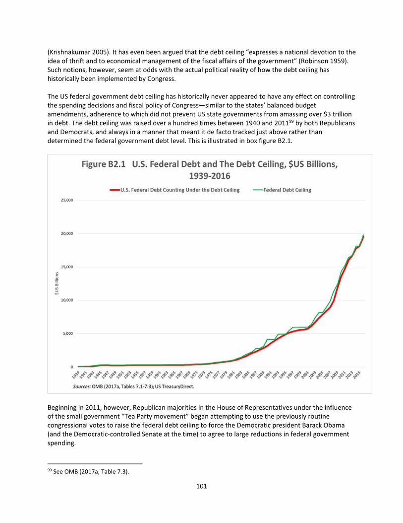
101  

(Krishnakumar 2005). It has even been argued that the debt ceiling “expresses a national devotion to the idea of thrift and to economical management of the fiscal affairs of the government” (Robinson 1959). Such notions, however, seem at odds with the actual political reality of how the debt ceiling has historically been implemented by Congress.  The US federal government debt ceiling has historically never appeared to have any effect on controlling the spending decisions and fiscal policy of Congress—similar to the states’ balanced budget amendments, adherence to which did not prevent US state governments from amassing over $3 trillion in debt. The debt ceiling was raised over a hundred times between 1940 and 201199 by both Republicans and Democrats, and always in a manner that meant it de facto tracked just above rather than determined the federal government debt level. This is illustrated in box figure B2.1.  

  Beginning in 2011, however, Republican majorities in the House of Representatives under the influence of the small government “Tea Party movement” began attempting to use the previously routine congressional votes to raise the federal debt ceiling to force the Democratic president Barack Obama (and the Democratic‐controlled Senate at the time) to agree to large reductions in federal government spending.  

                                                            99 See OMB (2017a, Table 7.3).  

102  

This political strategy of “fiscal chicken” threatening to push the US federal government into default unless their political demands were/are met has repeatedly led to brief crises around the time when the debt ceiling must be increased and in 2011 caused the United States to lose its AAA credit rating (Standard & Poor’s 2011). To date, however, there has not been a serious adverse reaction in the market for Treasury bonds, signaling that market participants continue to have faith in the willingness (and ability) of the US federal government to pay its debts.  The current federal government debt ceiling is $20.1 trillion, but Congress has repeatedly suspended the law—the last time in September 2017 by three months until December 8, 2017, at which time on December 9 the debt limit will automatically increase to account for obligations incurred by the federal government during the period of suspension.100 Congress as a result has to vote again in early December 2017 to either raise the debt ceiling further or maintain the current suspension of the debt ceiling.  

End box. 

 

12 Competitively Distributed Federal Government TIGER Grants to States 

A recurring theme in this paper has been how each major war or economic crisis faced by the United States has led to significant changes to and increases in federal government funding for US states. So too with the American Recovery and Reinvestment Act (ARRA), which in early 2009 provided a substantial short‐term fiscal stimulus to the US economy in the midst of the Great Recession. While it is probably too early to comprehensively evaluate the lasting effects of ARRA on intragovernmental funding relations, it is already clear that President Obama’s signature fiscal stimulus plan introduced several important and innovative vehicles through which federal government funding can continue to flow to the US states.  

Probably the most prominent one is the Department of Transportation’s (DOT) Transportation Investment Generating Economic Recovery, or TIGER Discretionary Grant program. In contrast to regular federal grants‐in‐aid programs to US states, which typically flow to the states inside relatively narrow subject silos demarcated by fixed federal government spending formulas, rigid compliance rules, and demands for state cofinancing, TIGER grants are distributed by the DOT on a simple competitive basis relying on only a few broad principles. Project applicants must make the case for their investment idea based on five long‐term outcomes: safety, economic competitiveness, state of good repair, quality of life, and environmental sustainability.  

TIGER grants imply a significant degree of federal government discretion over which states and what causes receive investment support. Again in contrast to regular transportation investment grants, which almost exclusively go to states’ departments of transportation or transit agencies, TIGER grants can also benefit any public entity across jurisdictions and fiscal years. This degree of federal government executive branch discretion is highly unusual for grants‐in‐aid funding but in principle allows for a rigorous merit‐based evaluation of projects aimed also at finding ways to ensure on‐time on‐budget completion of projects. On the other hand, this very high degree of funding discretion is likely to make TIGER grant funding subject to significant changes when a new administration takes office. It is also unlikely that Congress will allow this funding model to expand dramatically, despite early positive results, as it would reduce its own ability to shape federal government transportation investments. 

                                                            100 See H.R. 601 at www.congress.gov/bill/115th‐congress/house‐bill/601.  

103 

References 

BEA (Bureau of Economic Analysis). Various years. Online National Income and Product Accounts (NIPA) database. Washington. Available at https://www.bea.gov/iTable/index_nipa.cfm

BLS (Bureau of Labor Statistics). Online Unemployment Database. Washington. Available at http://data.bls.gov/pdq/querytool.jsp?survey=ln.  

Buchanan, James M. 1963. The Economics of Earmarked Taxes. Journal of Political Economy 71, no. 5 (October): 457–69. 

Burkhead, Jesse. 1956. Government Budgeting. New York: John Wiley & Sons. 

CBO (Congressional Budget Office). 2010. Fiscal Stress Faced by Local Governments. Washington. Available at www.cbo.gov/sites/default/files/111th‐congress‐2009‐2010/reports/12‐09‐municipalities_brief.pdf  

CBO (Congressional Budget Office). 2015a. Federal Debt and the Statutory Limit, August 2015. Washington. Available at www.cbo.gov/sites/default/files/114th‐congress‐2015‐2016/reports/50739‐FederalDebt.pdf  

CBO (Congressional Budget Office). 2015b. The Status of the Highway Trust Fund and Options for Paying for Highway Spending. Testimony by Deputy Assistant Director for Microeconomic Studies Chad Shirley Before the US House Committee on Ways and Means, Washington, June 17. Available at www.cbo.gov/sites/default/files/114th‐congress‐2015‐2016/reports/50298‐TransportationTestimony_1.pdf  

CBO (Congressional Budget Office). 2016. Approaches to Making Federal Highway Spending More Productive. Washington. Available at www.cbo.gov/publication/50150.  

CRS (Congressional Research Service). 2015. The Debt Limit: History and Recent Increases. Washington. Available at www.senate.gov/CRSpubs/d2c8f833‐9796‐4b3e‐9462‐6b1755ef463d.pdf.  

Department of Labor. 2017. Comparison of State Unemployment Insurance Laws. Washington. Available at https://workforcesecurity.doleta.gov/unemploy/pdf/uilawcompar/2017/complete.pdf  

Delpla, Jacques, and Jakob von Weizsacker. 2011. Eurobonds: The Blue Bond concept and its implications. Available at www.europarl.europa.eu/document/activities/cont/201103/20110321ATT15948/20110321ATT15948E

N.pdf.

Ellis, Joseph J. 2000. Founding Brothers: The Revolutionary Generation. Knopf Doubleday Publishing Group. 

English, William B. 1996. Understanding the Costs of Sovereign Default: American State Debts in the 1840s. American Economic Review 86, no. 1: 259–75. 

104  

 EU Council. 2014. Council Decision of 26 May 2014 on the system of own resources of the European Union. Available at http://eur‐lex.europa.eu/legal‐content/EN/TXT/PDF/?uri=CELEX:32014D0335&from=EN.  European Commission. 2015. EU Budget 2014. Financial Report. Available at  http://ec.europa.eu/budget/financialreport/2014/lib/financial_report_2014_en.pdf.   European Commission. 2016. DG Budget EU Expenditure and Revenue Data 2000‐2015. Available at http://ec.europa.eu/budget/library/biblio/documents/2015/internet‐tables‐2000‐2015.xls.    Federal Reserve Board. 1933. Twentieth Annual Report of the Federal Reserve Board 1933. Available at https://fraser.stlouisfed.org/files/docs/publications/arfr/1930s/arfr_1933.pdf#page=12   Follette, Glen, and Byron Lutz. 2010. Fiscal Policy in the United States: Automatic Stabilizers, Discretionary Fiscal Policy Actions, and the Economy. Available at www.federalreserve.gov/pubs/feds/2010/201043/201043pap.pdf.  Gale, William G., and Aaron Krupkin. 2016. Financing State and Local Pension Obligations: Issues and Options. Washington: Brookings Institution. Available at www.brookings.edu/wp‐content/uploads/2016/07/PB‐Pension‐shortfalls‐and‐SL‐budgets.pdf.  Gallup. 2016. June Wave 2—Final Topline. Available at www.gallup.com/file/poll/193406/160701Proud.pdf.   GAO (General Accounting Office). 1993. Balanced Budget Requirements: State Experiences and Implications for the Federal Government. Washington. Available at www.gao.gov/assets/80/78648.pdf.   GAO (Government Accountability Office). 2011. State and Local Governments: Knowledge of Past Recessions Can Inform Future Federal Fiscal Assistance. Washington. Available at http://www.gao.gov/products/GAO‐11‐401.   GAO (Government Accountability Office). 2012. Debt Limit: Analysis of 2011‐2012 Actions Taken and Effect of Delayed Increase on Borrowing Costs. Washington. Available at www.gao.gov/assets/600/592832.pdf.   High‐Level Group on Own Resources. 2017. Future Financing of the EU Final Report and Recommendations of the High Level Group on Own Resources. Available at http://ec.europa.eu/budget/mff/hlgor/library/reports‐communication/hlgor‐report_20170104.pdf  IMF (International Monetary Fund). 2013. Toward a Fiscal Union for the Euro Area. IMF Staff Discussion Note SDN/13/09. Washington. Available at www.imf.org/external/pubs/ft/sdn/2013/sdn1309.pdf.  Kandel, William A. 2015. US Citizenship and Immigration Services (USCIS) Functions and Funding. Washington: Congressional Research Service. Available at www.fas.org/sgp/crs/homesec/R44038.pdf.   

105  

Kirk, Robert S., and William J. Mallett. 2016. Funding and Financing Highways and Public Transportation. CRS Report R44674. Washington: Congressional Research Service. Available at https://fas.org/sgp/crs/misc/R44674.pdf.   Kirkegaard, Jacob F. 2015a. Economic Governance Structures in the United States. Available at http://www.europarl.europa.eu/RegData/etudes/STUD/2015/542668/IPOL_STU(2015)542668_EN.pdf   Kirkegaard, Jacob F. 2015b. Toward a European Migration and Mobility Union. PIIE Policy Brief 15‐23. Washington: Peterson Institute for International Economics. Available at https://piie.com/publications/policy‐briefs/toward‐european‐migration‐and‐mobility‐union.    Krisnakumar, Anita S. 2005. In Defense of the Debt Limit Statute. Harvard Journal on Legislation 42: 135–85.  McAdoo, William G. 1931. Crowded Years: The Reminiscences of William G. McAdoo. Boston, MA: Houghton‐Mifflin Company.  Mysak, Joseph. 2010. Bond Default is About Too Much Debt, Too Little Time. Available at www.bloomberg.com/news/articles/2010‐07‐21/bond‐default‐means‐too‐much‐debt‐too‐little‐time‐commentary‐by‐joe‐mysak   NASBO (National Association of State Budget Officers). 2015. Budget Processes in the States (Spring). Available at https://higherlogicdownload.s3.amazonaws.com/NASBO/9d2d2db1‐c943‐4f1b‐b750‐0fca152d64c2/UploadedImages/Reports/2015%20Budget%20Processes%20‐%20S.pdf.   NASBO (National Association of State Budget Officers). 2016. State Expenditure Report 2014‐16. Available at https://higherlogicdownload.s3.amazonaws.com/NASBO/9d2d2db1‐c943‐4f1b‐b750‐0fca152d64c2/UploadedImages/SER%20Archive/State%20Expenditure%20Report%20(Fiscal%202014‐2016)%20‐%20S.pdf.   NASBO (National Association of State Budget Officers). 2017. The Fiscal Survey of the States (Spring). Available at https://higherlogicdownload.s3.amazonaws.com/NASBO/9d2d2db1‐c943‐4f1b‐b750‐0fca152d64c2/UploadedImages/Fiscal%20Survey/NASBO%20Spring%202017%20Fiscal%20Survey%20(S).pdf.   NCSL (National Conference of State Legislatures). 2010. State Balanced Budget Provisions. NCSL Fiscal Brief. Available at http://www.ncsl.org/documents/fiscal/StateBalancedBudgetProvisions2010.pdf.   New York State Comptroller. 2015. New York’s Balance of Payments in the Federal Budget. Available at https://osc.state.ny.us/reports/budget/2015/fed_budget_fy2013.pdf   OMB (Office of Management and Budget). 2016. Budget Analytical Perspectives, Chapter 26 Trust Funds and Federal Funds. Washington. Available at www.gpo.gov/fdsys/pkg/BUDGET‐2017‐PER/pdf/BUDGET‐2017‐PER‐7‐2.pdf.   OMB (Office of Management and Budget). 2017a. Online Historical US Budget Database. Washington. Available at www.whitehouse.gov/omb/budget/Historicals.  

106  

OMB (Office of Management and Budget). 2017b. Composition of Social Insurance and Retirement Receipts and of Excise Taxes: 1940–2021. Available at www.gpo.gov/fdsys/pkg/BUDGET‐2017‐TAB/xls/BUDGET‐2017‐TAB‐3‐4.xls.   OMB (Office of Management and Budget). 2017c. Federal Receipts: 13. Tax Expenditures. Washington. Available at www.whitehouse.gov/sites/whitehouse.gov/files/omb/budget/fy2018/ap_13_expenditures.pdf.   OECD (Organization for Economic Cooperation and Development). 2013. United States Country Specific EPL Score. Paris. Available at www.oecd.org/els/emp/United%20States.pdf   Perkins, Frances. 1935. Report to the President of the Committee on Economic Security. Committee on Economic Security. Available at www.ssa.gov/history/reports/ces.html.  Pew Charitable Trust. 2016. State Retiree Healthcare Liabilities. Available at www.pewtrusts.org/en/research‐and‐analysis/issue‐briefs/2016/05/state‐retiree‐health‐care‐liabilities   Powell, Fred W. 1939. Control of Federal Expenditures: A Documentary History, 1775‐1794. Washington: Brookings Institution.  Robinson, Marshall A. 1959. The National Debt Ceiling: An Experiment in Fiscal Policy. Washington: Brookings Institution.  Rolph, Earl, and George Break. 1961. Public Finance. New York: Ronald Press Co.  Standard & Poor’s. 2011. United States of America Long‐Term Rating Lowered To 'AA+' On Political Risks And Rising Debt Burden; Outlook Negative. Research Update. Global Credit Portal. Available at www.washingtonpost.com/wp‐srv/politics/documents/spratingreport_080611.pdf?tid=a_inl.  Studenski, Paul, and Herman Edward Krooss. 1952. Financial History of the United States. New York: McGraw‐Hill Book Company, Inc.  Tax Foundation. 1955. Earmarked State Taxes. New York.  Tax Foundation. 2013. US Federal Individual Income Tax Rates History, 1862‐2013 (Nominal and Inflation Adjusted Brackets. Available at https://taxfoundation.org/us‐federal‐individual‐income‐tax‐rates‐history‐1913‐2013‐nominal‐and‐inflation‐adjusted‐brackets/.   US Census. 1949. Historical Statistics of the United States 1789–1945: A Supplement to the Statistical abstract of the United States. Washington: US Department of Commerce. Available at www2.census.gov/prod2/statcomp/documents/HistoricalStatisticsoftheUnitedStates1789‐1945.pdf   US Census. 2015. 2014 State and Local Government Summary Financial Tables by Level of Government and State. Washington. Available at https://factfinder.census.gov/faces/tableservices/jsf/pages/productview.xhtml?pid=SLF_2014_00A1&prodType=table  

107  

US Treasury. Various years. Annual Reports of the Secretary of the Treasury. Washington. Available at https://fraser.stlouisfed.org/title/194.   US Treasury. 2015. Monthly Statement of the Public Debt of the United States, July 31. Washington. Available at https://www.treasurydirect.gov/govt/reports/pd/mspd/2015/opds072015.pdf.  Wallis, John Joseph, Richard Sylla, and Arthur Grinath III. 2004 Sovereign Debt and Repudiation: The Emerging Market Debt Crisis in the U.S. States: 1839‐1843. NBER Working Paper 10573 (September). Cambridge, MA: National Bureau of Economic Research.   Williamson, Samuel H. 2014. The Annual Real and Nominal GDP for the United States, 1790‐2013. MeasuringWorth. Available at www.measuringworth.com/usgdp/#.   Yilen, Hou, and Daniel L. Smith. 2006. A Framework for Understanding State Balanced Budget Requirement Systems: Reexamining Distinctive Features and an Operational Definition. Public Budgeting and Finance 26, no. 3 (September): 22–45.     

108  

3  Federalizing a Central Bank: A Comparative Study of the Early Years of the Federal Reserve and the European Central Bank  Jérémie Cohen‐Setton and Shahin Vallée  Introduction 

Most, if not all, currency regimes are stable when general political and economic conditions are stable. 

Only in times of distress are they truly tested and the question surrounding their stability and 

sustainability is answered. The global financial crisis of 2007–09 and the subsequent recession exposed 

deep flaws in the Maastricht architecture. Many of these flaws have been highlighted in academic 

research, accepted by the policymaking community, and have led to some momentum to correct them. 

But relatively little has been said about the ways the structure and operation of the Eurosystem might 

be changed to strengthen and improve the sustainability of the euro area.101  

If anything, the crisis has revealed that national borders in monetary policy controversies remain 

relevant and that national central banks (NCBs) have not yet become mere branch offices of a 

federalized central bank (Lokdam 2017). This paper will show that the United States encountered many 

of the same challenges in its monetary architecture in the first 22 years of the US Federal Reserve 

System. Like the ECB Statutes and the provisions of the European Treaties, the Federal Reserve Act of 

1913 did not prescribe how the Federal Reserve should conduct monetary policy and respond to panics. 

To the extent that the Act provided guiding principles, these were flawed and implied that central bank 

liquidity ought to be reduced rather than increased in times of stress. The Federal Reserve Act also did 

not explicitly state how losses by the 12 regional Federal Reserve banks (FRBs) would be covered by the 

central fiscal authority, thereby reinforcing the doom loop between the real economy and the banking 

sector within each district.  

In the wake of the Great Depression of the 1930s, the Federal Reserve was reformed and given 

considerably greater power to act as a lender of last resort (LOLR). The federal government clarified that 

FRBs, if faced with important losses, would not have to be recapitalized by the member banks of their 

                                                            Jérémie Cohen‐Setton is a research fellow at the Peterson Institute for International Economics. Shahin Vallée is a PhD candidate at the European Institute at the London School of Economics. He is also senior economist at Soros Fund Management. The authors thank Barry Eichengreen, Gabriele Giudice, Daniel Heller, Mirzha De Manuel, Jacob Funk Kirkegaard, and Hjalte Lokdam for useful comments and feedback, as well as Didrich Berge for exceptional research assistance and Helen Hillebrand for copyediting. The authors are also grateful to Roberto A. De Santis for sharing updated data. 101 The Eurosystem comprises the European Central Bank (ECB) and the national central banks (NCBs) of those countries that have adopted the euro. 

109  

own districts but by the US Treasury.102 Thus, it was not the establishment of the Federal Reserve in 

1913 but the Great Depression that transformed the United States into a fully functioning monetary 

union and organized the fundamental compact between the central bank and the federal government.  

The Federal Reserve was within the federal government but independent. In contrast, the European 

Central Bank seems to have been thought out under the specific context of a central bank without a 

state (Zilioli and Selmayr 2001), in some way achieving Friedrich Hayek's (1976) idea of denationalizing 

money, or at least making it disconnected from the sovereign (Issing 2000). The central bank is no longer 

within government. Rather, it is next to it, but withholds certain prerogatives of the state.  

Ten years after the start of the Great Recession, the ECB has not gone through a similar aggiornamento. 

The relationship between the central bank and its sovereign(s) was left deliberately unsettled by the 

Maastricht Treaty. Against the backdrop of redenomination fears that have failed to completely 

disappear (figure 1), this clarification seems even more necessary in Europe now than in the United 

States then. In any decentralized monetary union, unclear prerogatives, guidelines, and policies about 

responsibilities for backstopping the banking system can turn localized financial risks into concerns 

about the sustainability of the currency union itself. But unlike the United States, the European context 

has some very unique features because of the existence of political calls to exit the common currency 

and of a mechanism for exiting the European Union. De facto, the ECB has thus had to operate in an 

environment where the probability of losing one member of the union is non‐zero despite being 

irrevocable de jure.103 

   

                                                            102 The Federal Reserve Act made it compulsory for national banks, that is, banks chartered and supervised by the Office of the Comptroller of the Currency (OCC), to become member banks of the Federal Reserve System and contribute, in proportion to their sizes, to the capital of the regional Federal Reserve bank in their respective districts. Other banks, such as state‐chartered banks and trust companies, could join the Federal Reserve System but were not required to do so. Those that did not join are referred to as nonmember banks.  103 To the best of the authors' knowledge, the Federal Reserve System never had to operate under such an environment. Money was at the center of political debates in the late 19th century in the United States with the Greenback and the Silver movements (Friedman and Schwartz 1963, Frieden 1997), but political calls for exiting the monetary union were dormant by the time the Federal Reserve System was established.  

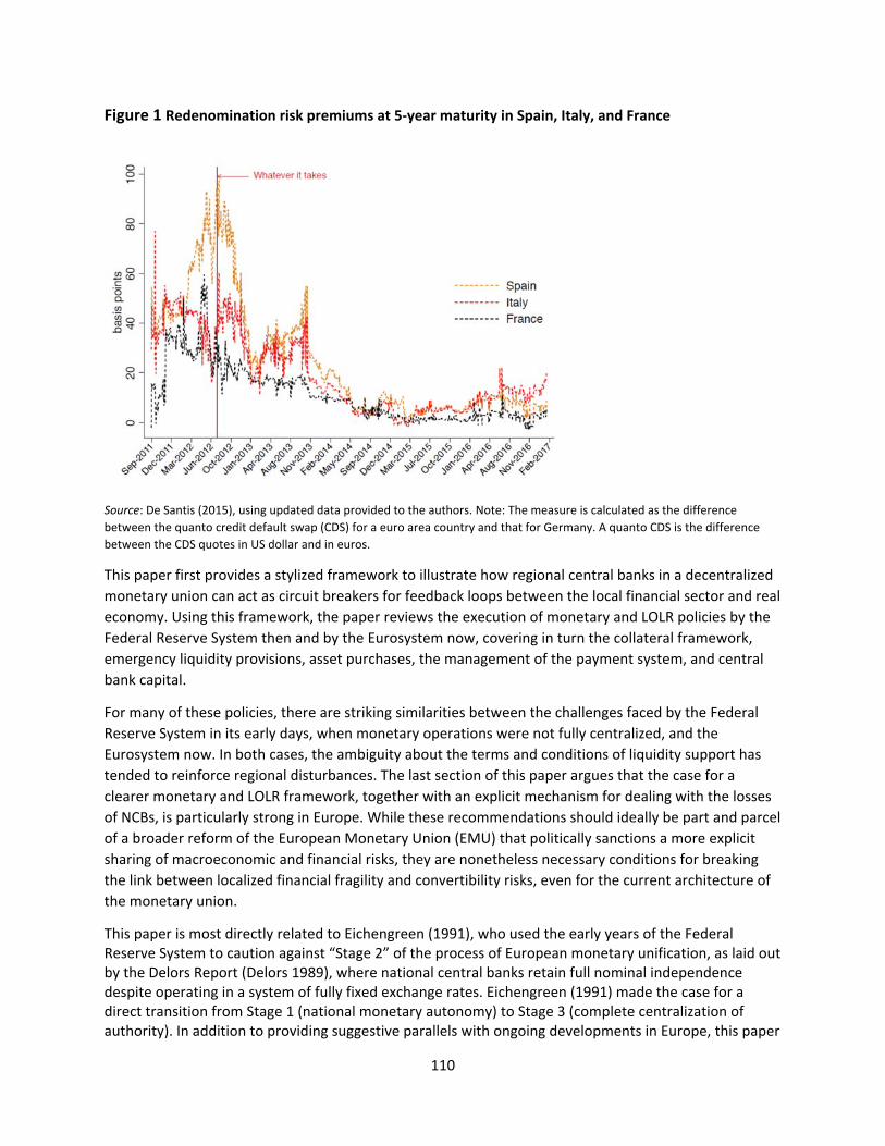
110  

Figure 1 Redenomination risk premiums at 5‐year maturity in Spain, Italy, and France  

 

Source: De Santis (2015), using updated data provided to the authors. Note: The measure is calculated as the difference 

between the quanto credit default swap (CDS) for a euro area country and that for Germany. A quanto CDS is the difference 

between the CDS quotes in US dollar and in euros. 

This paper first provides a stylized framework to illustrate how regional central banks in a decentralized 

monetary union can act as circuit breakers for feedback loops between the local financial sector and real 

economy. Using this framework, the paper reviews the execution of monetary and LOLR policies by the 

Federal Reserve System then and by the Eurosystem now, covering in turn the collateral framework, 

emergency liquidity provisions, asset purchases, the management of the payment system, and central 

bank capital.  

For many of these policies, there are striking similarities between the challenges faced by the Federal 

Reserve System in its early days, when monetary operations were not fully centralized, and the 

Eurosystem now. In both cases, the ambiguity about the terms and conditions of liquidity support has 

tended to reinforce regional disturbances. The last section of this paper argues that the case for a 

clearer monetary and LOLR framework, together with an explicit mechanism for dealing with the losses 

of NCBs, is particularly strong in Europe. While these recommendations should ideally be part and parcel 

of a broader reform of the European Monetary Union (EMU) that politically sanctions a more explicit 

sharing of macroeconomic and financial risks, they are nonetheless necessary conditions for breaking 

the link between localized financial fragility and convertibility risks, even for the current architecture of 

the monetary union.  

This paper is most directly related to Eichengreen (1991), who used the early years of the Federal Reserve System to caution against “Stage 2” of the process of European monetary unification, as laid out by the Delors Report (Delors 1989), where national central banks retain full nominal independence despite operating in a system of fully fixed exchange rates. Eichengreen (1991) made the case for a direct transition from Stage 1 (national monetary autonomy) to Stage 3 (complete centralization of authority). In addition to providing suggestive parallels with ongoing developments in Europe, this paper 

111  

and Eichengreen (1991) have in common the idea that stabilization tends to suffer when NCBs retain national considerations in their policies to maximize welfare. The papers, however, differ in their emphasis of the change that happened in the 1930s. While Eichengreen (1991) emphasizes the centralization of decision making, this paper highlights the compact between the central bank and its sovereign that was made explicit and the mechanisms for ensuring automatic par clearance across the 12 Federal Reserve banks (FRBs) that were improved. 

 The Conceptual Framework 

Regional feedback loops and the role of regional central banks 

The interaction between the balance sheets of the national banking system and the sovereign sector is 

well known. This “feedback loop” has led to a broad set of reflections about necessary reforms of the 

euro area’s financial architecture to reduce the way in which sovereigns and banks weigh on one 

another (Posen and Véron 2009). In 2012, heads of states and government agreed to establish a 

“banking union,” precisely with the intention of cutting this loop. Five years later, however, it remains 

unclear if, when completed, these reforms will be enough to completely break this link.  

More importantly, this understanding of the vicious loop between banks and their respective sovereigns 

neglects the important role the monetary authority plays in deflecting or intensifying the interaction 

between localized financial fragility and convertibility risks. In a monetary union, where the 

implementation of monetary policy is partly decentralized and central bank balance sheets are not 

consolidated, the monetary authorities can, in fact, be drawn into this vicious loop if they are seen as 

extensions of their regional economies or sovereigns.  

As shown by Gelpern and Véron (2017), local sovereigns did not play much of a role in this deadly 

embrace in the early years of the Fed or even before, in part because sovereign assets sitting on banks’ 

balance sheets were not as important as local private assets (figure 2). Instead, fears about the quality 

of bank assets in a region mostly stemmed from the high exposure of local banks to their nondiversified 

local economies. In the 1920s, banks typically held about 70 percent of their portfolios in loans (figure 

2).104 Given that the local private banking sector owned the FRBs, these regional feedback loops also 

flowed through the central bank’s balance sheet. In this set up where central banks become integral to 

regional feedback loops, the perception of the regional central bank’s solvency and the absence of an 

explicit mechanism for sharing risks associated with losses at the Federal level become key.  

  

 

 

   

                                                            104 This pattern is not specific to banks that are members of the Federal Reserve System. Table A‐3 of All Banks Statistics 1896‐1955 in Board of Governors of the Federal Reserve System (1959) shows that the same pattern applies for state‐chartered banks, which were mostly nonmember banks. 

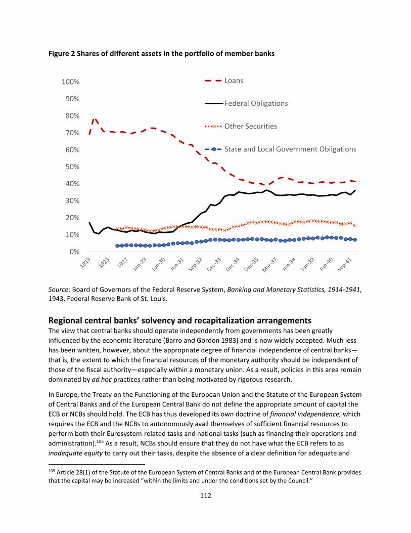
112  

Figure 2 Shares of different assets in the portfolio of member banks 

 

Source: Board of Governors of the Federal Reserve System, Banking and Monetary Statistics, 1914‐1941, 1943, Federal Reserve Bank of St. Louis. 

 Regional central banks’ solvency and recapitalization arrangements  The view that central banks should operate independently from governments has been greatly 

influenced by the economic literature (Barro and Gordon 1983) and is now widely accepted. Much less 

has been written, however, about the appropriate degree of financial independence of central banks—

that is, the extent to which the financial resources of the monetary authority should be independent of 

those of the fiscal authority—especially within a monetary union. As a result, policies in this area remain 

dominated by ad hoc practices rather than being motivated by rigorous research.  

In Europe, the Treaty on the Functioning of the European Union and the Statute of the European System 

of Central Banks and of the European Central Bank do not define the appropriate amount of capital the 

ECB or NCBs should hold. The ECB has thus developed its own doctrine of financial independence, which 

requires the ECB and the NCBs to autonomously avail themselves of sufficient financial resources to 

perform both their Eurosystem‐related tasks and national tasks (such as financing their operations and 

administration).105 As a result, NCBs should ensure that they do not have what the ECB refers to as 

inadequate equity to carry out their tasks, despite the absence of a clear definition for adequate and 

                                                            105 Article 28(1) of the Statute of the European System of Central Banks and of the European Central Bank provides that the capital may be increased “within the limits and under the conditions set by the Council.” 

0%

10%

20%

30%

40%

50%

60%

70%

80%

90%

100% Loans

Federal Obligations

Other Securities

State and Local Government Obligations

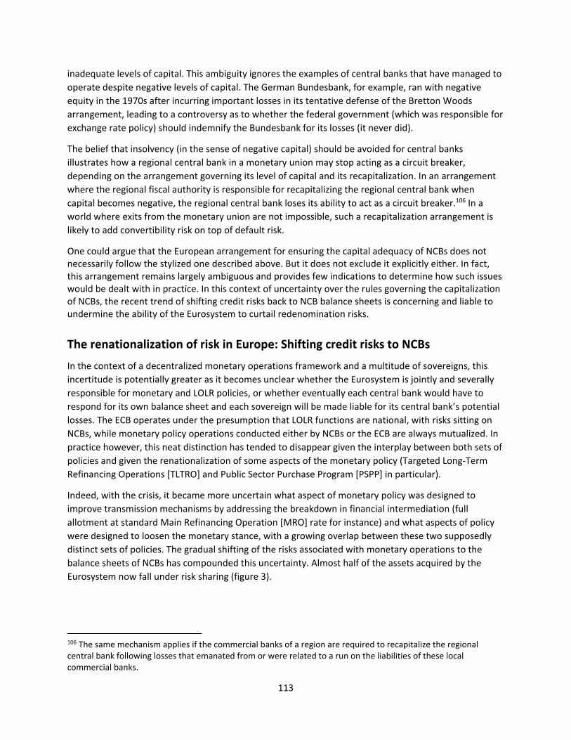
113  

inadequate levels of capital. This ambiguity ignores the examples of central banks that have managed to 

operate despite negative levels of capital. The German Bundesbank, for example, ran with negative 

equity in the 1970s after incurring important losses in its tentative defense of the Bretton Woods 

arrangement, leading to a controversy as to whether the federal government (which was responsible for 

exchange rate policy) should indemnify the Bundesbank for its losses (it never did).  

The belief that insolvency (in the sense of negative capital) should be avoided for central banks 

illustrates how a regional central bank in a monetary union may stop acting as a circuit breaker, 

depending on the arrangement governing its level of capital and its recapitalization. In an arrangement 

where the regional fiscal authority is responsible for recapitalizing the regional central bank when 

capital becomes negative, the regional central bank loses its ability to act as a circuit breaker.106 In a 

world where exits from the monetary union are not impossible, such a recapitalization arrangement is 

likely to add convertibility risk on top of default risk.  

One could argue that the European arrangement for ensuring the capital adequacy of NCBs does not necessarily follow the stylized one described above. But it does not exclude it explicitly either. In fact, this arrangement remains largely ambiguous and provides few indications to determine how such issues would be dealt with in practice. In this context of uncertainty over the rules governing the capitalization of NCBs, the recent trend of shifting credit risks back to NCB balance sheets is concerning and liable to undermine the ability of the Eurosystem to curtail redenomination risks.  

 The renationalization of risk in Europe: Shifting credit risks to NCBs 

In the context of a decentralized monetary operations framework and a multitude of sovereigns, this 

incertitude is potentially greater as it becomes unclear whether the Eurosystem is jointly and severally 

responsible for monetary and LOLR policies, or whether eventually each central bank would have to 

respond for its own balance sheet and each sovereign will be made liable for its central bank’s potential 

losses. The ECB operates under the presumption that LOLR functions are national, with risks sitting on 

NCBs, while monetary policy operations conducted either by NCBs or the ECB are always mutualized. In 

practice however, this neat distinction has tended to disappear given the interplay between both sets of 

policies and given the renationalization of some aspects of the monetary policy (Targeted Long‐Term 

Refinancing Operations [TLTRO] and Public Sector Purchase Program [PSPP] in particular).  

Indeed, with the crisis, it became more uncertain what aspect of monetary policy was designed to 

improve transmission mechanisms by addressing the breakdown in financial intermediation (full 

allotment at standard Main Refinancing Operation [MRO] rate for instance) and what aspects of policy 

were designed to loosen the monetary stance, with a growing overlap between these two supposedly 

distinct sets of policies. The gradual shifting of the risks associated with monetary operations to the 

balance sheets of NCBs has compounded this uncertainty. Almost half of the assets acquired by the 

Eurosystem now fall under risk sharing (figure 3).  

   

                                                            106 The same mechanism applies if the commercial banks of a region are required to recapitalize the regional central bank following losses that emanated from or were related to a run on the liabilities of these local commercial banks. 

114  

Figure 3 Risk‐sharing arrangements for assets held by the Eurosystem  

 

LTRO = Longer‐Term Refinancing Operations; MRO = Main Refinancing Operation; MLF = Marginal Lending Facility; CSPP = 

Corporate Sector Purchase Program; ABSPP = Asset‐Backed Securities Purchase Program; SMP = Securities Market Program; 

PSPP = Public Sector Purchase Program; ACC = Additional Credit Claims Note: Full risk sharing = LTRO + MRO + MLF + CSPP + 

ABSP + SMP +0.2*PSPP. No risk sharing = ELA + 0.8*PSPP. This overestimates full risk sharing as liquidity obtained using ACC is 

considered risk shared, which it was not. 

Source: ECB. 

One can view this renationalization of risk as secondary, so long as money can flow throughout the monetary union and to the extent that the Eurosystem can, in principle, function even if the equity of one or all of its NCBs is negative. But this view clearly depends on the notion that free movement of capital will never be challenged, that the size of Target 2 imbalances will never be restrained, and that no country will decide to break from the monetary union.  

 The deregionalization of risk in the United States: Removing credit risks from regional FRBs 

These questions are not, however, fundamentally new or unique to the euro area. The uncertainty 

about the underlying nature of the relationship between the 12 regional FRBs, the Federal Reserve 

Board, and the federal government was critical in the first 22 years of the Federal Reserve System. In 

fact, it was only after the height of the banking crises of the Great Depression that these questions were 

addressed decisively at a time when there was a compelling need to convince the public that the banks 

were safe. After the bank holiday was declared, the government only had a week to examine the 

solvency of thousands of banks; only the financially naive would have believed that all the reopened 

banks were indeed solvent (Wigmore 1987). It was thus necessary to warrant the provision of unlimited 

liquidity by FRBs to all reopened banks. 

0

0.5

1

1.5

2

2.5

3

3.5

Trillions of eu

ros

No risk‐sharing

Full risk‐sharing

115  

This effectively transferred credit risks to the balance sheets of the regional FRBs. By extending large 

amounts of liquidity to banks in shaky conditions, the regional FRBs would more likely than not face 

important losses. The guarantee from the federal government took the form of a telegram, dated March 

11, 1933 from Treasury Secretary William Woodin to New York Fed Governor George Harrison. In the 

telegram, it was reported that President Franklin D. Roosevelt had indeed committed to compensate all 

FRBs in case of losses. Roosevelt said that “it [was] inevitable that some losses may be made by the 

Federal Reserve Banks in loans to their member banks […] [but] there is definitely an obligation on the 

Federal Government to reimburse the 12 regional Federal Reserve Banks for losses which they may make 

on loans made under these emergency powers. I do not hesitate to assure you that I shall ask the 

Congress to indemnify any of the 12 Federal Reserve banks for such losses. I am confident that Congress 

will recognize its obligation to these Federal Banks should the occasion arise, and grant such request” 

(Silber, 2009).  

This precedent was of historic proportion. In fact, beyond helping with the immediate need of reopening banks and making sure that FRBs would provide enough liquidity in the face of possible new bank runs and a collapse in the money multiplier, the telegram established that there was no reason for FRBs to act in an uncooperative manner to protect their reserves. The lesson from this episode is that in the absence of such a Rooseveltian commitment, doubts about the strength of the underpinning compact that ties regional central banks with the sovereign can be a tremendous force of financial fragility. This paper therefore argues that a similar Rooseveltian moment is needed in the euro area to effectively and completely transnationalize monetary operations and that this is inextricably linked to a form of fiscal and political underwriting of central bank responsibilities.  

 A Comparative Analysis of the Early Years of the Federal Reserve System and the Eurosystem 

The central bank’s objectives and monetary operations fall within two broad categories: policies 

designed to manage the money supply and policies designed to repair transmission mechanisms in the 

event of crises. For the most part, these latter operations fall under the LOLR name tag. Yet beyond this 

clear description and the potentially neat institutional arrangements that can be set up around it, the 

interaction between the two forms of monetary operations is, in practice, much stronger.  

This section reviews the execution of monetary operations by both the Federal Reserve System and the Eurosystem in their early years of operations. The discussion starts with the collateral framework and then turns to asset purchases, emergency liquidity provisions, and the payment system. It concludes by discussing the question of losses and central bank capital.   

Collateral policy 

The US experience then 

The availability of eligible collateral was highly uneven across regions during the Great Depression in the 

United States. Influenced by the real bills doctrine, the Federal Reserve Act provided for a particularly 

narrow definition of eligible collateral. Only “notes, drafts, and bills of exchange arising out of actual 

commercial transactions” and only those bills with a term to maturity of 90 days or less (180 days for 

agricultural loans) were eligible for discount operations. As commerce and industry came to a near halt 

116  

during the Great Depression, “self‐liquidating” commercial loans were lacking at the very time when 

there was the greatest need for liquidity in the country (Hawtrey 1932, 130).  

In contrast to the general claim by Friedman and Schwartz (1963) that “there was ample [at all times] 

eligible paper in the portfolios of member banks,” Chandler (1971) shows that the availability of 

collateral was greatly heterogeneous across regions. Many banks had exhausted their supply of eligible 

collateral even before the first banking panic of the Great Depression in 1930 in the Boston, 

Philadelphia, and Cleveland districts (Chandler 1971, table 15.3).107 Similar data for later periods in the 

Depression are not available, but there is no reason to believe that the supply of collateral in these 

regions improved over time, as it decreased for the United States as a whole by 4.6 percent between the 

end of 1929 and the end of 1931. 

The response of Federal Reserve banks to the deterioration in the quality of collateral also intensified 

this situation. McKinney (1960) notes that “during the early years of the depression all of the Federal 

Reserve banks […] were requiring substantial amounts of excess collateral.” This procyclicality in the 

administration of the discount window certainly intensified the pressure on banks. The government 

responded to these challenges first outside of the Federal Reserve by creating the Reconstruction 

Finance Corporation (RFC), which opened for business on February 2, 1932, and stood ready to lend on 

sound assets of every kind.108 The surge of bank borrowing from the RFC suggests, in fact, that the 

quantity of eligible collateral was a binding constraint (Chandler 1971). It also rapidly endeavored to 

change the Federal Reserve’s discounting operations as Congress passed the Glass‐Steagall Act, which 

relaxed rules for discount window lending.109  

Under Title IV, Section 13 (3) of the Glass‐Steagall Act of 1932, Federal Reserve banks were authorized 

to lend on the basis of any sound collateral to member banks and to nonmember banks, but only under 

“exceptional and exigent circumstances” (Friedman and Schwartz 1963) and if eligible paper had been 

exhausted. These final restrictions would only be removed with the Banking Act of 1935 (Board of 

Governors of the Federal Reserve System 1937). Only then were Federal Reserve banks thus truly 

allowed to make advances on any security type and whenever desired. 

In 1937, these provisions were incorporated into Regulation A, which governs the discount operations of 

the 12 regional Federal Reserve banks (Regulation A).110 The new regulation was prefaced by a 

statement of general principles, which underlies the significant changes in the discount philosophy of 

the Federal Reserve before and after the Great Depression. Recognizing the procyclical bias of the 

previous period, Regulation A outlines that credit should instead be extended liberally “at times when 

the value of assets held by banks may be decreasing because of a downward turn in the nation’s 

business and a decrease in the national income” (Board of Governors of the Federal Reserve System 

1937). 

                                                            107 In these districts, Chandler (1971) shows that 40 percent of member banks had eligible assets amounting to less than 10 percent of their total loans and investments and were thus unable to borrow from the Federal Reserve System. 108 The legislation was approved on January 22, 1932, and the RFC opened for business on February 2, 1932. 109 The Glass‐Steagall Act of 1932 should not be confused with the Banking Act of 1933, which is commonly referred to the “Glass‐Steagall Act.”  110 Regulation A can be found in the Federal Reserve Bulletin, October 1937 (Board of Governors of the Federal Reserve System 1937). 

117  

 

The European experience now 

This American experience illustrates how normal monetary operations and the collateral framework 

influence the ability to undertake monetary operations in times of crisis. In the United States, the real 

bills doctrine that governed standard monetary operations came to be a central impediment to the 

Federal Reserve’s LOLR. In Europe, in large part because the lessons from Bagehot (1873) have been 

widely accepted by European central banks since the 19th century, this was in principle less of an issue. 

However, the ECB’s collateral framework has evolved though the crisis and experienced important 

changes. 

Indeed, when the European Monetary Institute was replaced by the European Central Bank, there was a 

general acceptance that while the national financial and banking sectors were very diverse, the direction 

of travel was one of gradual convergence, which would gradually force convergence of discount policies 

of the national central bank and increase risk sharing by the European Central Bank. Nowhere is this 

more visible than in the establishment and evolution the collateral framework policy of the ECB, which, 

given the largely bank‐based nature of the European financial system, is the cornerstone of central bank 

policy in the euro area. 

In 2001, at the launch of EMU, the collateral framework was effectively two‐tiered—the first tier was 

based on harmonized eligibility criteria and the second tier was national. As early as 2003 however, the 

ECB set out a process intended to gradually converge the two‐tier system towards a single collateral 

framework because “the Eurosystem recognizes that the heterogeneity of the assets included in the tier 

two lists may not ensure a level playing field for counterparties.” A final homogeneous collateral 

framework under a single list emerged by January 2007, not really because of concerns about monetary 

policy transmission but rather because of concerns about the competitive level playing field. 

While the ECB only accepted high quality collateral, the question of the credit rating of the collateral was 

never made a criterion during the establishment of this single, centralized and risk‐shared collateral 

framework. The view was that the ECB should retain full discretion and not make eligibility conditional 

on a discretionary assessment made by rating agencies outside of its control. In November of 2005, 

however, following the violation of the Growth and Stability Pact (SGP) by France and Germany, the ECB 

Governing Council changed this practice. When the ECB attempted to warn European governments 

about the consequences of overspending and strengthen the role of market discipline, it decided that it 

would only accept bonds with at least a rating of A– from one or more of the rating agencies as 

collateral.  

While this decision had no immediate consequences because all member states were comfortably rated 

above this threshold, it signaled the ECB's desire to increase market discipline to substitute for fiscal 

rules that had failed to create fiscal prudence. At a press conference, then ECB president Jean‐Claude 

Trichet argued that this was a compromise with smaller consequences than the other alternatives on 

the table, which would have made eligibility or haircuts directly linked to the abeyance to the 

prescriptions of the SGP.111  

                                                            111 “We were told very often by parts of the economists’ community [that we were] too benign, too positive vis‐à‐vis government paper, that we should practice a lot of haircuts and so forth, or practice haircuts combined with 

118  

It was not until October 15, 2008, that the question of the collateral framework became a central policy 

discussion again. Following the failure of Lehman Brothers, the ECB took the immediate and temporary 

decision not only to provide liquidity on a fixed rate full allotment basis but also to considerably expand 

the pool of collateral by accepting bank bonds and lowering the rating threshold from A– to BBB–. The 

€870 billion increase in the pool of eligible collateral allayed many of the liquidity concerns in the euro 

area, and the ECB was celebrated as having reacted to this global shock forcefully as an effective LOLR. 

This action provided a clear indication that the ECB was prepared to alter its operational and collateral 

framework to perform its LOLR function in the most effective way.  

This demonstrated flexibility concerning eligible collateral stands in contrast with the apparent rigidity 

with which the collateral framework was operated in 2010 when the crisis became European. The ECB 

signaled then that it would not change its collateral framework to accommodate member states that 

might lose access to refinancing operations because of downgrades. This reaction intensified market 

stress and accelerated downgrades in a procyclical and circular manner, as the rating agencies 

themselves considered the loss of refinancing access as a critical element of their rating outlook. To this 

day, it is hard to explain why the reaction function was so different during these two episodes.  

This rigid treatment of the collateral framework however had profound consequences—not only on the 

ability of governments to fund themselves but also on the stability and liquidity position of their banking 

systems, which in turn increased their need for emergency liquidity funding. This episode reinforced the 

perception of a somewhat unpredictable reaction function towards financial stability. 

When the ECB eventually introduced a new dose of flexibility in its framework by allowing a certain degree of collateral differentiation across jurisdictions,112 this change happened together with the quid pro quo that these credit claims were to be kept on the balance sheet of NCBs rather than mutualized. With hindsight, this appears to have been a far less aggressive and generous attitude than the one prevailing at the inception of the global financial crisis. It is not clear what motivated these decisions. But it represented for the Eurosystem a first step backwards from the unicity and full mutualization of the risks associated with its monetary operations inside the euro area.  

 Asset purchases 

The US experience then  

In the United States, Federal Reserve holdings of government securities only became the principal 

source of currency in circulation in the 1930s, a process that thus displaced the importance of the 

discount facility. The departure from the real bills doctrine and the development of capital markets 

                                                            the Stability and Growth Pact implementation—or non‐implementation. We thought that this was not appropriate. We said that it was not appropriate for us to invent a new sanction that would apply for non‐compliance with the Stability and Growth Pact via this collateral mechanism. We felt that we should not do that.” European Central Bank, "Introductory statement with Q&A," press conference, December 1, 2015, https://www.ecb.europa.eu/press/pressconf/2005/html/is051201.en.html (accessed November 8, 2017).  112 NCBs were allowed to accept Additional Credit Claims (ACC) as eligible collateral “based on the specific eligibility criteria and risk control measures set by NCBs”, which are not eligible under the single list. See Mario Draghi and Vítor Constâncio, "Introductory statement to the press conference (with Q&A)," press conference, December 8, 2011, European Central Bank, http://www.ecb.int/press/pressconf/2011/html/is111208.en.html (accessed November 29, 2017). 

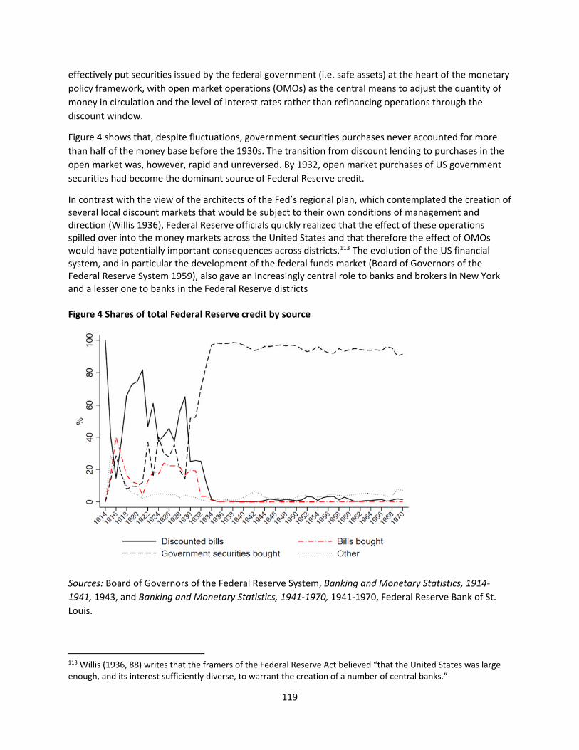
119  

effectively put securities issued by the federal government (i.e. safe assets) at the heart of the monetary 

policy framework, with open market operations (OMOs) as the central means to adjust the quantity of 

money in circulation and the level of interest rates rather than refinancing operations through the 

discount window.  

Figure 4 shows that, despite fluctuations, government securities purchases never accounted for more 

than half of the money base before the 1930s. The transition from discount lending to purchases in the 

open market was, however, rapid and unreversed. By 1932, open market purchases of US government 

securities had become the dominant source of Federal Reserve credit.  

In contrast with the view of the architects of the Fed’s regional plan, which contemplated the creation of several local discount markets that would be subject to their own conditions of management and direction (Willis 1936), Federal Reserve officials quickly realized that the effect of these operations spilled over into the money markets across the United States and that therefore the effect of OMOs would have potentially important consequences across districts.113 The evolution of the US financial system, and in particular the development of the federal funds market (Board of Governors of the Federal Reserve System 1959), also gave an increasingly central role to banks and brokers in New York and a lesser one to banks in the Federal Reserve districts   Figure 4 Shares of total Federal Reserve credit by source 

 

Sources: Board of Governors of the Federal Reserve System, Banking and Monetary Statistics, 1914‐

1941, 1943, and Banking and Monetary Statistics, 1941‐1970, 1941‐1970, Federal Reserve Bank of St. 

Louis. 

                                                            113 Willis (1936, 88) writes that the framers of the Federal Reserve Act believed “that the United States was large enough, and its interest sufficiently diverse, to warrant the creation of a number of central banks.” 

120  

Already in 1923, an Open Market Investment Committee was created to coordinate asset purchases, but 

the arrangement was, however, voluntary and nonbinding.  The Committee evolved over the years, but 

it was only with the Banking Act of 1933 that created the Federal Open Market Committee (FOMC) that 

its decisions became binding on the Reserve banks (Richardson, Komai, and Gou 2013).  

Federal Reserve banks were then prohibited from purchasing or selling securities at their own initiatives, while the FOMC was empowered to instruct Reserve banks to sell or transfer any securities held or purchased to a joint System Open Market Account (Friedman and Schwartz 1963; FRB 1933, 302). As open market operations became the primary tool for providing central bank money, the allocation of purchases across the 12 Federal Reserve banks also became a central mechanism to equalize exposures and minimize tensions within the payment system between them. The exact formula to allocate purchases has evolved over time (McCalmont 1963), but the principle of sharing reserves depending on needs remains. In fact, the allocation of purchases is still made based on the annual settlement of interdistrict balances and the underlying idea that gold certificate holdings should be equalized.114   The European experience now 

In Europe also, asset purchases have become central to the monetary policy toolkit but for different 

reasons. After hitting the zero‐lower bound on nominal interest rates, nonstandard measures became 

necessary to loosen the monetary policy stance, in addition to simply improving the transmission 

mechanisms (Cohen‐Setton and Vallée 2013). The first program of sovereign debt purchases (the 

Securities Market Program, or SMP) was announced on May 10, 2011. While there was no formal link 

between the launch of SMP and the political agreement on the creation of the European Financial 

Stability Facility (EFSF), the sequencing (EFSF first, SMP second) suggests that the ECB behaved 

strategically (Henning 2015), waiting for governments to first mutualize some of the financial risk before 

acting itself. 

The program was entirely discretionary and targeted countries whose sovereign debt markets were at 

risk (Greece, Ireland, Spain, Portugal, and Italy). As the likelihood of a debt restructuring in Greece 

increased, the ECB expressed its opposition by arguing that this would require a recapitalization of the 

central bank and emphasizing its super seniority status. Because ECB purchases started to be seen as a 

source of subordination of private sector creditors in the event of restructuring, the program became a 

source of destabilization and was interrupted.  

It was only in the summer of 2012 with the announcement of its Outright Monetary Transactions (OMT) 

program that the ECB clearly signaled not only the potential unlimited nature of the purchases 

(“whatever it takes”), but also the explicit pari passu nature of the ECB’s purchases. Although not always 

clearly formulated, this suggested an important shift in ECB doctrine, and the link between the balance 

sheet, potential losses, and recapitalization was clearly avoided. In fact, by focusing on the existence of 

redenomination risk, the ECB insisted on the endogenous nature of these risks and the fact that by 

                                                            114 In April of each year, the average daily balance on each Reserve bank’s interdistrict settlement account during the preceding 12 months is calculated. Based on the resulting netting of these balances, the Board and the Markets Group at the New York Reserve Bank calculate the amount each Bank should have in its gold certificate account to equal the System average of gold certificates to Federal Reserve notes outstanding. If a decrease in a Bank's gold certificate account is needed, it is achieved by increasing the Bank's participation in the SOMA. If an increase in a Bank's gold certificate account is needed, it is achieved by decreasing the Bank's participation in the SOMA (Board of Governors of the Federal Reserve System 2017, p. 105).  

121  

intervening, the ECB was enhancing the quality of its balance sheet and reducing aggregate risks in the 

system. OMT could, however, only be undertaken in the context of a financial assistance program in a 

bid not only to secure political and financial underwriting of some of the risks associated with the 

operation but also somewhat strategically to ensure an arm’s length relationship with the member state 

needing assistance. 

The ECB eventually moved away from some of the key parameters underlying OMT with the 

announcement of a new program of asset purchases (Public Sector Purchase Program) in 2015. While 

the PSPP was no longer presented as an instrument to repair the transmission channel but rather as a 

true monetary policy operation (Cohen‐Setton and Vallée 2013), the ECB introduced a very clear 

limitation in the risk sharing by decentralizing the purchases and the risks. Only 20 percent of the PSPP 

related purchases would be risk shared. The quid pro quo inside the ECB Governing Council was 

therefore that the program could be very large, but the degree of risk mutualization would have to be 

limited.  

This quid pro quo reflected an important underlying tradeoff at work inside the Governing Council 

between the importance of the size of the program on the one hand and the extent to which 

renationalizing risk would signal distrust in the long‐term sustainability of the single currency on the 

other. Indeed, the only underlying reason to seek to keep purchased assets on the NCBs’ balance sheets 

is the concern over not only their solvency but more importantly what a breakup of the monetary union 

would entail. Despite the monetary union being de jure irrevocable, ECB president Mario Draghi argued 

that the “decision [was made to] mitigate the concerns that many participating countries in the euro 

area have about the unintended fiscal consequences of potential developments in the future”.115 

The ECB felt that this concession was only minor because while assets wouldn’t be risk shared, in practice the monetary liabilities created through the implementation of the program would remain fungible across the euro area so long as capital would flow freely across borders. In this context, it is critical to assess whether the perfect fungibility of money can be maintained under all possible circumstances and whether the provisions and constraints on Emergency Liquidity Assistance (ELA) played a pivotal role in this respect.  

 Emergency liquidity  

The US experience then 

The period between the establishment of the Federal Reserve and the Great Depression has until recently 

received little attention in the literature on banking panics. That relative absence is mostly unsurprising, 

given that major national banking runs were absent during these years (Jalil 2015). Interestingly, this 

period has now become central in the study of the role of central banks as LOLR and the effects of 

deposit insurance. Despite the absence of national banking runs, the period has the advantage of 

providing regional variation in the number and intensity of local banking runs, regional variations in the 

LOLR policies employed by the different FRBs, and regional variations in deposit insurance schemes at the 

state level. Table 1 displays the location and time of major local banking panics between 1921 and 1929, 

                                                            115 Mario Draghi, "Introductory statement to the press conference (with Q&A)," January 22, 2015, European Central Bank, https://www.ecb.europa.eu/press/pressconf/2015/html/is150122.en.html (accessed on November 14, 2017). 

122  

whether deposit insurance schemes existed in the states affected, and the different FRBs in charge of 

providing emergency liquidity.  

Exploiting a dataset from the Federal Deposit Insurance Corporation (FDIC) on bank suspensions and 

newspaper evidence, Davidson and Ramirez (2014) identify 14 local banking panics over the years 1921–

29. Given the numerous agricultural shocks over this period (e.g., collapse in cotton prices in 1920–21, a 

fruit fly infestation in Florida in April 1929), it is not surprising that these local panics happened mostly in 

agricultural states. What is more interesting is the varying incidence of these crises depending on the 

regional FRB responsible for the affected jurisdiction. In a system dominated by liquidationist views, the 

Federal Bank of Atlanta was unique in championing monetary activism (Gamble 1989, Richardson and 

Troost 2009, White 2015). Several papers have exploited this discontinuity to identify the effect of 

monetary intervention during panics. In a paper that extends the approach of Richardson and Troost 

(2009) of comparing the performance of banks in counties straddling the Atlanta Federal Reserve district 

border,116 Jalil (2015) finds that monetary intervention by the Atlanta Fed reduced bank suspensions by 

about one third, providing what is certainly the cleanest evidence of the causal impact of LOLR 

interventions.  

The US experience also provides an interesting perspective on the link between emergency liquidity 

provision and deposit insurance. Following the "Panic of 1907," eight states enacted insurance systems 

for their state‐chartered banks. Using regression evidence, Davidson and Ramirez (2014) find that panics 

were less likely to occur in states that had deposit insurance, thereby limiting the need for LOLR 

intervention. In fact, among the states with deposit insurance, table 1 shows that local banking panics 

only occurred in South Dakota (1916–27) and Kansas (1909–29) for the period covered by these 

authors.117 While one would need to look in more detail at the amount of monetary intervention for 

each of these panics, it is also likely that the substitution between deposit insurance and LOLR 

operations operated at the intensive margin, i.e., that LOLR liquidity was less ample when deposit 

insurance played its role. 

   

                                                            116 The Richmond, St. Louis, Cleveland, and Dallas FRBs all share a border with the Atlanta FRB. Richardson and Troost (2009) compare the performance of Mississippi banks in counties straddling the Atlanta and St. Louis district border. Jalil (2015) extends this same approach to the other borders of the Atlanta FRBs.  117 The dates in parentheses correspond to the period in which the respective deposit insurance schemes were in operation. These dates are taken from Table 28, “Participation of Operating Banks in Stata Deposit Insurance Systems, December 31, 1908–1930” in FDIC (1956). The other states with deposit insurance were Oklahoma (1908–23), Texas (1910–27), Nebraska (1911–30), Mississippi (1914–30), North Dakota (1917–29), and Washington (1917–21). 

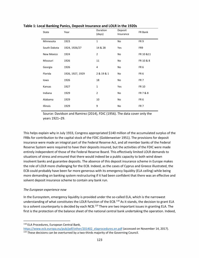
123  

Table 1: Local Banking Panics, Deposit Insurance and LOLR in the 1920s  

State  Year Duration 

(days) 

Deposit 

Insurance FR Bank 

Minnesota  1923  1  No  FR 9 

South Dakota  1924, 1926/27  14 & 28  Yes  FR9 

New Mexico  1924  2  No  FR 10 &11 

Missouri  1926  11  No  FR 10 & 8 

Georgia  1926  4  No  FR 6 

Florida  1926, 1927, 1929  2 & 19 & 1  No  FR 6 

Iowa  1926  18  No  FR 7 

Kansas  1927  1  Yes  FR 10 

Indiana  1929  2  No  FR 7 & 8 

Alabama  1929  10  No  FR 6 

Illinois  1929  9  No  FR 7 

Source: Davidson and Ramirez (2014), FDIC (1956). The data cover only the 

years 1921–29. 

 

This helps explain why in July 1933, Congress appropriated $140 million of the accumulated surplus of the 

FRBs for contribution to the capital stock of the FDIC (Goldenweiser 1951). The provisions for deposit 

insurance were made an integral part of the Federal Reserve Act, and all member banks of the Federal 

Reserve System were required to have their deposits insured, but the activities of the FDIC were made 

entirely independent of those of the Federal Reserve Board. This effectively limited LOLR demands to 

situations of stress and ensured that there would indeed be a public capacity to both wind down 

insolvent banks and guarantee deposits. The absence of this deposit insurance scheme in Europe makes 

the role of LOLR more challenging for the ECB. Indeed, as the cases of Cyprus and Greece illustrated, the 

ECB could probably have been far more generous with its emergency liquidity (ELA ceiling) while being 

more demanding on banking system restructuring if it had been confident that there was an effective and 

solvent deposit insurance scheme to contain any bank run. 

 

The European experience now 

In the Eurosystem, emergency liquidity is provided under the so‐called ELA, which is the narrowest 

understanding of what constitutes the LOLR function of the ECB.118 As it stands, the decision to grant ELA 

to a solvent counterparty is decided by each NCB.119 There are two important issues in granting ELA. The 

first is the protection of the balance sheet of the national central bank undertaking the operation. Indeed, 

                                                            118 ELA Procedures, European Central Bank, https://www.ecb.europa.eu/pub/pdf/other/201402_elaprocedures.en.pdf (accessed on November 14, 2017). 119 These decisions can be overturned by a two‐thirds majority of the Governing Council. 

124  

in every instance (known to the authors), member states have guaranteed to cover any losses stemming 

from the national central bank’s ELA exposure and were encouraged by the ECB to do so to protect the 

national central bank’s balance sheet. Second, while ELA in principle protects the balance sheet of the 

ECB, it increases the liabilities of the Eurosystem and, in the event of cross‐border capital flight, increases 

the exposure of the Eurosystem to the central bank extending ELA via the rise in Target 2 balances.  

However, as Whelan (2016) showed in the specific case of Ireland, ELA often played a critical role in a 

country’s ability to resist financial distress. In Greece and Cyprus, where Greek covered bonds and Cypriot 

government bonds were downgraded and became ineligible for normal refinancing operations, the day‐

to‐day liquidity management of these banking systems relied on ELA. As such, the introduction of a 

discretionary binding cap made avoiding some form of capital controls and payment restrictions 

impossible.  

On March 16, 2013, after months of negotiations between the European Commission, the ECB, and the 

International Monetary Fund—known as the Troika—the Eurogroup decided to introduce a levy on 

deposits, including insured deposits, to raise several billion euros and reduce both the financing needs of 

Cypriot banks and therefore the size of the financial assistance program and associated ELA risk to the 

Eurosystem. This measure ended up being reversed the next day in a Eurogroup teleconference, and 

subsequently replaced via a new program for insured depositors. But the second agreement, which did 

not impose a bail‐in or levy on depositors, nonetheless led to the introduction of capital controls because 

capital flight had set in and ELA remained capped. The conclusion of a financial assistance program by the 

IMF and the European Commission—which covered a restructuring of the entire banking system—did not 

lead the ECB to authorize further extension of ELA, which remained limited at the same level and 

therefore required prolonged restrictions to payments and cash withdrawals.  

There was initially a debate about the legal basis for such capital controls, given that free movement of 

capital is a fundamental principle of the European Union and is codified in Article 63 (1) of the Treaty on 

the Functioning of the European Union (TFEU), which bans restrictions on the “movement of capital” and 

“payments” in and out of EU member states. After the government of Cyprus introduced capital controls, 

the European Commission, as guardian of the Treaties, argued that in certain circumstances member 

states could introduce such restrictions120 under Article 65 of the TFEU, which reserves the right of 

member states “to take measures which are justified on grounds of public policy or public security.” The 

European Court of Justice (ECJ) never formally ruled on the case against the Cypriot program, but it 

obviated the question of capital controls by ruling that a program ordered and agreed by the European 

Stability Mechanism (ESM) could not create any legal responsibilities for the European Commission or the 

ECB.121 This reasoning, combined with a 2006 case where the ECJ had already ruled that the guarantee of 

                                                            120 European Commission, "Statement by the European Commission on the capital controls imposed by the Republic of Cyprus," press release, March 28, 2013, http://europa.eu/rapid/press‐release_IP‐13‐298_en.htm (accessed on November 14, 2017). 121Court of Justice of the European Union, Arrêt de la Cour, September 20, 2016, http://curia.europa.eu/juris/document/document_print.jsf;jsessionid=9ea7d0f130d504473e56958f4762b81ebec23d12cc86.e34KaxiLc3eQc40LaxqMbN4Pa3qOe0?doclang=FR&text=&pageIndex=0&part=1&mode=DOC&docid=183547&occ=first&dir=&cid=619833 (accessed November 14, 2017). 

125  

a service of general interest could constitute an overriding justification to curtail the free movement of 

capital,122 offered constructive legal support to introduce capital controls in the European Union.  

Regardless of whether the ECB directly or indirectly encouraged the introduction of capital controls to reduce its financial exposure and the extent of its liquidity support to the Cypriot banking system, this precedent was momentous: It made the case for the possible imperfect fungibility of Eurosystem monetary liabilities.  

The payment system 

The US experience then 

Prior to 1914 when the Federal Reserve opened its doors, interregional settlements took place through a 

correspondent banking system in which banks in one region held balances with banks in other regions. In 

this setting, the failure of banks on either side of the transaction could disrupt interregional payments. 

The Federal Reserve System was established and organized into districts to address this instability, among 

other things. Its Interdistrict Settlement System would guarantee smooth and reliable settlement of the 

claims of one region on another. There was no possibility of a Reserve bank failing in the manner of a 

correspondent bank, and therefore no possibility of one region defaulting on its claims to another 

(Cohen‐Setton 2017). 

But par clearance as mandated in the Federal Reserve Act was not automatic, as there were, in fact, 

constraints on the ability of regional Reserve banks to settle 1:1 between each other. Every FRB and not 

just the system as a whole was required to hold gold reserves against its liabilities. In principle, a FRB with 

a gold ratio approaching the minimum thresholds could shrink its liabilities to restore its gold ratio, but 

this type of procyclical adjustment would be disruptive (Eichengreen et al. 2015).  

Instead, in the first 20 years of the Fed, FRBs adjusted by pooling their gold reserves, mostly through 

regional rediscounts. While there is disagreement in the literature as to whether this mutual assistance 

among FRBs was seamless (Hackley 1973, Eichengreen et al. 2015) or grudging (White 2015), the 

disagreements shed light on how an imperfect framework for mutualizing risk can interfere with 

monetary operations. The first known episode of interregional tensions occurred during the 1920–21 

recession, which predominantly affected agricultural regions. White (2015) shows that the LOLR actions 

of the Atlanta Fed were vigorously contested by the Cleveland Fed. The Federal Reserve Board relayed 

the views that the Atlanta Fed was too lenient in its lending policy and threatened to expose to the public 

its precarious reserve position. In ambiguous terms, a member of the Board even suggested that it 

“would be more inclined to allow the reserve of the Atlanta Bank [to] show a depreciation” than to allow 

further interdistrict rediscounts (White 2015).  

In early 1933, another episode of tension emerged. A speculative attack against the New York Fed’s gold 

reserves led to a reduction of its gold ratio towards the statutory limit. The New York Fed made a request 

to the Chicago Fed to rediscount government securities, but the latter refused. The Board, which had the 

authority to interfere and force such rediscounting initially refused to do so, leading the New York Fed to 

                                                            122 European Commission Legal Service, "C‐282/04 and C‐283/04 Commission v Netherlands, judgment of 28.9.2006, Free movement/ Internal market –'Golden shares'," September 28, 2006, http://ec.europa.eu/dgs/legal_service/arrets/04c282_en.pdf (accessed on November 14, 2017). 

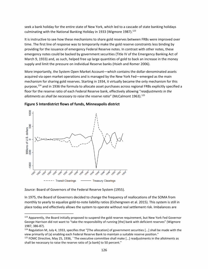
126  

seek a bank holiday for the entire state of New York, which led to a cascade of state banking holidays 

culminating with the National Banking Holiday in 1933 (Wigmore 1987).123 

It is instructive to see how these mechanisms to share gold reserves between FRBs were improved over 

time. The first line of response was to temporarily make the gold reserve constraints less binding by 

providing for the issuance of emergency Federal Reserve notes. In contrast with other notes, these 

emergency notes could be backed by government securities (Title IV of the Emergency Banking Act of 

March 9, 1933) and, as such, helped free up large quantities of gold to back an increase in the money 

supply and limit the pressure on individual Reserve banks (Hsieh and Romer 2006). 

More importantly, the System Open Market Account—which contains the dollar‐denominated assets 

acquired via open market operations and is managed by the New York Fed—emerged as the main 

mechanism for sharing gold reserves. Starting in 1934, it virtually became the only mechanism for this 

purpose,124 and in 1936 the formula to allocate asset purchases across regional FRBs explicitly specified a 

floor for the reserve ratio of each Federal Reserve bank, effectively allowing “readjustments in the 

allotments as shall be necessary to raise the reserve ratio” (McCalmont 1963).125  

Figure 5 Interdistrict flows of funds, Minneapolis district 

 

Source: Board of Governors of the Federal Reserve System (1955).  

In 1975, the Board of Governors decided to change the frequency of reallocations of the SOMA from 

monthly to yearly to equalize gold‐to‐note liability ratios (Eichengreen et al. 2015). This system is still in 

place today and effectively allows the system to operate without real settlement risk. Imbalances are 

                                                            123 Apparently, the Board initially proposed to suspend the gold reserve requirement, but New York Fed Governor George Harrison did not want to “take the responsibility of running [the] bank with deficient reserves” (Wigmore 1987, 386‐87). 124 Regulation M, July 4, 1933, specifies that "[The allocation] of government securities [...] shall be made with the view primarily of (a) enabling each Federal Reserve Bank to maintain a suitable reserve position." 125 FOMC Directive, May 25, 1936, ``The executive committee shall make […] readjustments in the allotments as shall be necessary to raise the reserve ratio of [a bank] to 50 percent.” 

127  

simply traded away via SOMA reallocations. As a result, while interdistrict imbalances are indeed settled 

and collateralized every year in April, this settlement is less reality than meets the eye, as reallocations in 

SOMA de facto provide the transfers of securities necessary to ensure that the settlement between the 

regional districts are minimal.126  

This can be seen from the summary of transactions of the Interdistrict Settlement Fund (ISF), which both 

record the losses and gains of funds due to transit clearings and those due to transfers for the 

government.127 When a check is drawn from a bank outside the district, the receiving bank sees a credit in 

its reserve account at its FRB, while the FRB in the other district decreases the reserve account of the 

sending bank. This transaction creates a claim for the receiving FRB and a liability for the sending FRB that 

are recorded in the ISF (Bowsher 1961). What figure 5 shows for the Minneapolis district between 1920 

and 1954 is that the movements in these two components move almost one to one in a compensating 

manner at the yearly frequency, thereby limiting much of the need for actual settlements.128  

This practice has, however, often been misunderstood and has led to calls to collateralize Target 2 

balances in Europe. But rather than constraining NCBs with Target 2 net liabilities, a convergence to the 

American system would be akin to the ECB undertaking asset purchases to limit Target 2 system 

imbalances by, for example, buying more than the capital key dictates in countries facing capital outflows 

and/or allocating these purchases to the balance sheets of the NCBs with capital inflows. 

 

The European experience now 

Target 2 is a centralized payment system operated by the Eurosystem. It is used both by central banks 

and commercial banks alike and provides the backbone of the domestic and cross‐country payment 

system; it is therefore inextricably connected to capital flows between countries. It is de facto a system by 

which NCBs provide credit to each other and is profoundly affected both by the open market operations 

as well as the refinancing operations of the Eurosystem.  

The operation of this payment system and the resulting target balances have however become a source 

of important policy debates over the years, as it is the most visible expression of financial flows and 

imbalances building up between euro area countries. This is not a new problem: It had been at the heart 

of a controversy in the 1990s when central bankers were to replace the system of the Very Short‐Term 

Financing Facility (VSTFF) that underpinned the workings of the Exchange Rate Mechanism (ERM). While 

the provision of liquidity was meant to be in principle unlimited, the Basle‐Nybord agreement at that time 

already stipulated clearly that “the provision of credit should not undermine the monetary policy of the 

central banks,” which offered an escape clause for the Bundesbank. EMU and Target 2 closed that door 

and practically forced the extension of unlimited target balances. But this has not removed the political 

economy tensions surrounding the extension of such credit balances.  

                                                            126 Wolman (2013) gives examples on how this is recorded in the balance sheets of the different regional FRBs. 127 The ISF was previously called the Gold Settlement Fund. ISF transactions do not include all interdistrict payments. Some are made in cash and some by checks that are cleared without going through the FRBs (Bowsher 1961). The statistical releases G.15 are available on FRASER for the period 1915–71. See https://fraser.stlouisfed.org/title/3932#480556.  128 The pattern is the same for the other districts. In fact, a panel regression of Treasury Transfers on Transit Clearing gives a coefficient of –0.96 with a t‐test statistic of –130.  

128  

The debate on Target 2 imbalances surfaced inside the ECB in February 2012 when a letter from 

Bundesbank president Jens Weidmann to ECB president Draghi was leaked to the press.129 It warned the 

ECB about the risks to its credibility if these imbalances were to grow further. The Bundesbank then 

explicitly proposed collateralizing these target imbalances to protect the creditor position of the 

Bundesbank in the Target system. This echoed calls made in Germany since 2011, most notably by Hans‐

Werner Sinn (e.g. Sinn 2012).130 The ECB's response was twofold; it defended the maintenance of the 

Target 2 settlement system as an absolute necessity enshrined in the Treaty, but it also conceded that the 

Target 2 imbalances reflected certain structural imbalances that could not be ignored.  

The Bundesbank went a step further in its 2011 annual report released in March 2012 by outlining that 

“parts of the negative TARGET2 balances might be transformed into actual balance sheet risks […] if a 

member state were to exit monetary union.” The Bundesbank proceeded to explain that the ECB could try 

to recover its claims on the departing NCB, including by the available collateral, but the residual claim and 

resulting loss for the ECB might need to be compensated through a capital increase that would be 

decided by the NCB based on a capital key majority. But the Bundesbank concluded that it nonetheless 

expected the “monetary union to persist in its current form.” 

Financial fragmentation and the tensions surrounding Target 2 continued to rise until the summer of 

2012, when the ECB’s announcement of OMT succeeded in triggering a reversal in capital flows. The ECB 

celebrated this improvement by pointing to the decline in Target 2 balances. This relative stabilization has 

not, however, fully abated the political uncertainty over EMU integrity. It is unclear whether a country 

that decides to leave the euro area could force the ECB to change its reaction function with respect to 

how it operates the settlement system. While the ECB can argue that the Maastricht Treaty clearly states 

that the fixing of exchange rates is "irrevocable" (Protocol No. 3), and that the character of the 

movement to a single currency is "irreversible" (Protocol No. 10), treaties can be revoked or changed. In 

addition, Article 50 of the TFEU provides a venue for leaving the European Union, which for an EMU 

member would also lead to exiting the single currency. It is therefore perfectly conceivable that politics 

would prompt reversibility. Indeed, the German Constitutional Court has recognized this much itself in a 

court ruling on the Maastricht Treaty in 1993 when it found that Germany could withdraw if the EMU 

came to challenge basic stability principles laid out in the Treaty.  

In some sense, the ECB recognized this in 2017 when President Draghi responded in a letter to Italian 

members of parliament on Target 2 balances by explaining that “If a country were to leave the 

Eurosystem, its national central bank’s claims on or liabilities would need to be settled in full.”131 This 

admission of the possible revocability of the monetary union forces the ECB to think of the political 

economy of the monetary union in somewhat different terms.  

 

                                                            129 Stefan Ruhkamp, "Die Bundesbank fordert von der EZB bessere Sicherheiten," Frankfurter Allgemeine Zeitung, February 29, 2012, http://www.faz.net/aktuell/wirtschaft/schuldenkrise‐die‐bundesbank‐fordert‐von‐der‐ezb‐bessere‐sicherheiten‐11667413.html (accessed on November 10, 2017). 130 Hans‐Werner Sinn, "Fed versus ECB: How Target debts can be repaid," March 10, 2012, VoxEU. 131 Letter available at https://www.ecb.europa.eu/pub/pdf/other/170120letter_valli_zanni_1.en.pdf?be6aea5c0aa3596d1d08149b510ea707 (accessed on November 29, 2017). 

129  

Central bank solvency 

The US experience then 

In the United States, each individual Federal Reserve bank is a separate legal entity with distinct private 

shareholders and individual balance sheets. There is no requirement in the Federal Reserve Act (FRA) for 

any mutualization of liabilities between these different shareholders, as they are responsible for 

covering their individual FRB’s liabilities “for all contracts, debts, and engagements of such bank [FRB] to 

the extent of the amount of their subscriptions to such stock at the par value thereof in addition to the 

amount subscribed, whether such subscriptions have been paid‐up in whole or in part.”132 

Initially, the FRA authorized FRBs to build up a surplus by retaining interest earned from their asset 

portfolio until it reached 40 percent of paid‐in capital of member banks. Net earnings beyond this 

threshold were to be transferred to the Treasury as a “franchise tax.” In 1919 the FRA was amended to 

allow surplus to be raised to 100 percent of subscribed capital. After the establishment of the FDIC, 

Congress abolished the franchise tax and allowed the Fed to retain all subsequent net earnings to 

rebuild surplus (Goodfriend 2014). 

To avoid negative equity or the need to be recapitalized by its shareholders, each of the 12 FRBs 

maintains two capital accounts—a paid‐in capital account and a surplus account. Under the FRA, 

member banks must subscribe to the stock of their respective FRB. The subscription is 6 percent of each 

member bank’s capital and surplus. Half of the subscription amount is paid‐in. The other half is on call 

by the Federal Reserve Board. FRBs also use what they call a capital surplus account to act as a cushion 

against losses. According to the Financial Accounting Manual for Federal Reserve Banks, the primary 

purpose of the surplus account is, indeed, to provide capital to supplement paid‐in capital for use in the 

event of loss.133 

This question of the Federal Reserve’s capital and risk tolerance became an important part of the 

discussion during the global financial crisis, when it was compelled to extend extraordinary liquidity and 

indirectly purchase assets to preserve financial stability even prior to the failure of Lehman Brothers. 

Indeed, as early as March 2008, the rescue of Bear Stearns and subsequently AIG led the Federal 

Reserve to use its powers as a LOLR. The creation of the Maiden Lane facilities (the Delaware Limited 

Liability Company to which the Federal Reserve offered long‐term loans to take over the troubled assets 

of Bear Stearns and AIG) was allowed under certain provisions of Section 13 (3) of the FRA. These 

provisions were later restricted by the Dodd‐Frank Act by preventing loans to a single corporation and 

thus preventing the Fed from using the same Maiden Lane approach in future crises. 

Interestingly, the Federal Reserve was uneasy with the risks undertaken and, in cooperation with the US 

Treasury, issued a joint communique offering not only political but also financial cover for the actions 

taken.134 The joint communique released on March 23, 2009, shortly after the start of the Fed's 

                                                            132 Federal Reserve Act, Section 2.4, “Liabilities of Shareholders of Reserve Banks,” as quoted by Stella (2009). 133 A 2002 analysis by the General Accounting Office (GAO 2002) shows that when FRBs had insufficient weekly earnings to absorb weekly losses between 1989 and 2001, they drew on their capital surplus accounts. 

 134  "The Role of the Federal Reserve in Preserving Financial and Monetary Stability Joint Statement by the Department of the Treasury and the Federal Reserve," March 23, 2009, 

130  

quantitative easing (QE) program, stressed the need for cooperation between the Federal Reserve and 

the Treasury during a financial crisis but sets out important caveats. It stressed the need for the Federal 

Reserve to intervene in credit markets not for allocating credit to the economy but to restore market 

functioning and ensure financial stability. It also stressed that the ``Treasury will seek to remove from the 

Federal Reserve's balance sheet, or to liquidate, the so‐called Maiden Lane facilities made by the Federal 

Reserve as part of efforts to stabilize systemically critical financial institutions,” thereby indicating a 

rather explicit political and financial backstop of the US Treasury behind the actions of the Federal 

Reserve.  

This experience and the tension that it created was the reason the US government was under great 

pressure to step in with the creation of the large Troubled Asset Relief Program (TARP)—initially 

budgeted at some $700 billion and in the end trimmed down to $430 billion—which played a critical role 

in ensuring financial stability over and above what the post‐1930s institutions (FDIC and Federal 

Reserve) could have achieved. The Treasury took over many of the responsibilities that would have 

otherwise fallen under the Federal Reserve’s extended LOLR role.  

 

The European experience now 

In May 2010—shortly after the launch of the SMP program and after the ECB had already faced serious 

losses in 2008 and proceeded with sharing them with no commotion—the ECB set out to shore up its 

capital. By a majority decision of the Governing Council, the ECB required a doubling of its capital from 

€5 billion to €10 billion to comfortably cover any potential losses arising from its operations. This 

decision was followed by stricter provisions preventing the transfer of profits from NCBs to national 

governments—which can only be undertaken after accumulated losses from previous years have been 

covered—thereby ensuring that the national central bank is not compelled by its government to transfer 

resources without the ECB's approval.  

In these discussions, the question of the financial independence of the ECB and the NCBs have become 

central. The notion of inadequate equity to carry out their missions was introduced but never clearly 

defined. In fact, it was always implicitly assumed that an adequate amount of equity would necessarily 

be positive, so the question of a central bank functioning with negative equity was never directly 

addressed. It was only in its 2010 annual Convergence Report (where the ECB assesses progress towards 

joining the single currency) that an explicit reference to this issue appeared: “[A]ny situation should be 

avoided whereby for a prolonged period an NCB’s net equity is below the level of its statutory capital or 

is even negative, including where losses beyond the level of capital and the reserves are carried over. 

Any such situation may negatively impact on the NCB’s ability to perform its ESCB‐related tasks but also 

its national tasks.” 

Interestingly, the experience of the Czech and Slovakian central banks—which have both carried 

negative equity since the late 1990s when they depegged and accrued large losses without apparent 

prejudice to performing their monetary functions—do not seem to challenge the ECB doctrine. In fact, 

the experience of the National Bank of Slovakia in the euro since 2009 shows that a central bank in 

deeply negative equity can perform all its related tasks. It was therefore quite surprising when the ECB 

                                                            https://www.federalreserve.gov/newsevents/pressreleases/monetary20090323b.htm (accessed on November 10, 2017).  

131  

insisted that the Czech National Bank (CNB) was not meeting all legal requirements to join the euro area 

in part because of its negative equity position. The CNB protested and argued that its negative equity 

position was in no way an obstacle to carry out its functions in full, and the CNB governor lambasted the 

ECB’s sudden singling out of the Czech central bank without mentioning Slovakia's as “an unjustified 

departure from the European Union’s equal treatment principle.”135 This should have opened an 

important debate of doctrine on the importance of capital for central banking purposes, but it has not. 

To the best of the authors' knowledge, the ECB gave the CNB no public response. The ECB’s advice on 

the matter thereby remains and has been included in every subsequent Convergence Report to the 

present. 

 

 

Box 1: The Search for a Euro Area Safe Asset136 

 Jeromin Zettelmeyer 

 

The “doom loop” between banks and sovereigns, in which sovereign troubles can induce banking sector 

instability, and vice versa, has been a hallmark of the Euro area crisis (Pisani‐Ferry 2014). In spite of the 

ongoing economic recovery and the creation of a European resolution framework that seeks to protect 

sovereigns from banking troubles, it remains relevant today. One reason for this is that banks remain 

largely unprotected from their sovereigns. The 2011‐12 Euro area debt crisis triggered a “repatriation” 

of sovereign debt to the domestic banking systems of countries such as Italy, Portugal and Spain (Figure 

1, see also Battistini et al. 2014 and Brutti and Sauré 2016). This creates an important channel through 

which sovereign risk can affect banks and ultimately the real economy (Schnabel and Schüwer 2016, 

Bocola 2016). 

                                                            135 Czech National Bank, "The Czech National Bank disagrees with the ECB Convergence Report," press release, May 12, 2010, https://www.cnb.cz/en/public/media_service/press_releases_cnb/2010/20100512_convergence.html (accessed on November 10, 2017). 136 This box draws on Leandro and Zettelmeyer (2017). I am grateful to Gabriele Giudice, Mirzha de Manuel, Jean Pisani‐Ferry and participants at seminar participants at the European Commission and for comments. 

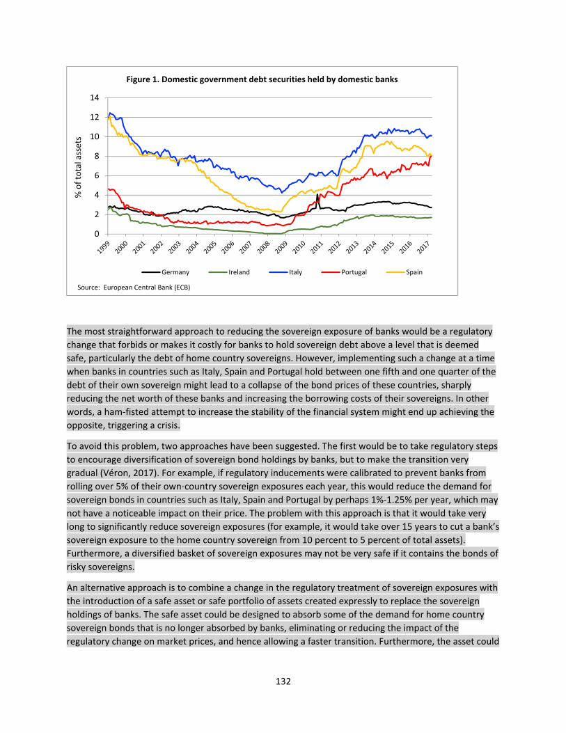
132  

 

 

The most straightforward approach to reducing the sovereign exposure of banks would be a regulatory 

change that forbids or makes it costly for banks to hold sovereign debt above a level that is deemed 

safe, particularly the debt of home country sovereigns. However, implementing such a change at a time 

when banks in countries such as Italy, Spain and Portugal hold between one fifth and one quarter of the 

debt of their own sovereign might lead to a collapse of the bond prices of these countries, sharply 

reducing the net worth of these banks and increasing the borrowing costs of their sovereigns. In other 

words, a ham‐fisted attempt to increase the stability of the financial system might end up achieving the 

opposite, triggering a crisis.  

To avoid this problem, two approaches have been suggested. The first would be to take regulatory steps 

to encourage diversification of sovereign bond holdings by banks, but to make the transition very 

gradual (Véron, 2017). For example, if regulatory inducements were calibrated to prevent banks from 

rolling over 5% of their own‐country sovereign exposures each year, this would reduce the demand for 

sovereign bonds in countries such as Italy, Spain and Portugal by perhaps 1%‐1.25% per year, which may 

not have a noticeable impact on their price. The problem with this approach is that it would take very 

long to significantly reduce sovereign exposures (for example, it would take over 15 years to cut a bank’s 

sovereign exposure to the home country sovereign from 10 percent to 5 percent of total assets). 

Furthermore, a diversified basket of sovereign exposures may not be very safe if it contains the bonds of 

risky sovereigns. 

An alternative approach is to combine a change in the regulatory treatment of sovereign exposures with 

the introduction of a safe asset or safe portfolio of assets created expressly to replace the sovereign 

holdings of banks. The safe asset could be designed to absorb some of the demand for home country 

sovereign bonds that is no longer absorbed by banks, eliminating or reducing the impact of the 

regulatory change on market prices, and hence allowing a faster transition. Furthermore, the asset could 

0

2

4

6

8

10

12

14

% of total assets

Figure 1. Domestic government debt securities held by domestic banks

Germany Ireland Italy Portugal Spain

Source:  European Central Bank (ECB)

133  

be made genuinely safe (comparable, say, to a German bund), assuaging fears that diversification might 

induce contagion risk.  

Initial proposals for Euro area safe assets envisaged “Eurobonds” that would be mutually guaranteed by 

Member States (De Grauwe and Moesen 2009, Bonnevay 2010). This idea failed to gain traction because 

of its potential for generating moral hazard (outside a fiscal union), and is essentially taboo today. In the 

meantime, however, there have been several proposals that dispense with guarantees. These include:  

“E‐bonds” issued by a senior public intermediary that simultaneously buys a diversified portfolio 

of Euro area sovereign bonds and passes its funding costs on to these sovereigns (see Monti 

2010). “Safety” is achieved both through diversification and the preferred creditor status of the 

intermediary.  

“ESBies”, which operate in the same way except that they dispense with seniority of the 

intermediary (Brunnermeier et al, 2011, 2017). Instead the debt instrument is issued in several 

tranches, with the tranching points (i.e. the “thickness” of the junior tranches) calibrated to 

make the senior tranche (the ESBie, or European senior bond) as safe as a German bund. Unlike 

E‐bonds, this proposal could also be implemented by many private intermediaries operating 

under a common rulebook.  

“National tranching”, which would also involve diversification and tranching, but in reverse 

order. National debt would be issued in two or more tranches (Wendorff and Mahle 2015). A 

diversified pool of the senior tranches (or an asset backed by such a pool) could be held by 

banks.  

Finally, Euro area debt issued by either a Eurozone budget (Ubide, 2015) or a leveraged Euro 

area sovereign wealth fund. This debt would be sustained by either a Euro‐area level tax (such 

as a corporate tax or small VAT) or by contributions from Member States.  

Leandro and Zettelmeyer (2017) evaluate these proposals based on: (1) the volume of safe assets that 

they could create; (2) their impact on fiscal discipline; (3) their impact on the liquidity of national debt 

markets; (4) redistributive effects; (5) the potential to introduce “mutualization through the back door”; 

(6) impact on average debt costs. The main results are as follows: 

First, all proposals could generate sufficient safe assets to replace (or very largely replace) sovereign 

bonds in bank balance sheets. This said, there is a large variation across proposals. National tranching 

would have the lowest yield in terms of volume, capable of generating senior asset pools (that is, 

diversified baskets of senior national debt tranches) worth about 15 percent of Euro area GDP, which is 

roughly the amount of sovereign debt securities in Euro area banks. A Euro area budget or leveraged 

wealth fund could generate much larger volumes if so desired but would require (at least initially) 

sufficiently large contributions to do so, perhaps in the order of 0.5% of Euro area GDP. Among the 

proposals involving intermediaries purchasing national debt, the ESBies can potentially create the 

largest volumes of safe assets, of perhaps up to 35 percent of Euro area GDP, but this would require 

buying up to 80 percent of the German and French debt markets. If the intermediary is not allowed to 

buy more than 50 percent of each country’s debt market, the most efficient way of generating European 

safe assets would be via the E‐bond approach, which could yield up to 25 percent of Euro area GDP in 

terms of safe assets generated. 

134  

Second, all proposals are potentially good for fiscal discipline in the sense that they would limit the spill‐

overs of sovereign debt restructuring to the real economy, and hence make it somewhat easier to refuse 

bail‐outs to sovereigns with unsustainable debts. One proposal – the E‐bonds – has an additional 

discipline‐creating effect because the preferred creditor status of the E‐bond intermediary may have the 

effect of increasing the marginal cost of debt issuance for countries that have reached their debt 

issuance limit to the E‐bond intermediary.  

Third, debt issuance by an EU budget or an EU sovereign wealth fund would leave national debt markets 

essentially unaffected (except for modestly shrinking their volume, on the assumption that total Euro 

area debt would remain unchanged). In contrast, national tranching would have a very severe impact on 

national markets, particularly if most sovereign tranches are held by banks for regulatory purposes, 

rendering them illiquid. Most debt trading in European debt markets would be junior national debt, 

likely implying greater price volatility and easier loss of market access. The E‐bond and ESBies proposals 

occupy an intermediate position: they would reduce the volume of tradable national debt, but could be 

designed to limit their purchases in a way that preserves national debt market liquidity. 

Fourth, assuming they work as intended, none of the proposals would lead to redistribution, with the 

notable exception of the E‐bond proposal (a Euro area budget might of course also lead to 

redistribution, but only if the expenditure side is designed to do so). In the E‐bond proposal, 

redistribution arises because the funding costs of the intermediary disproportionately depend on its 

exposure to specific members, but are distributed across all members in according to their portfolio 

weights. Simulations indicate that the total redistribution could be in the order of €10 billion over five 

years, mostly at the expense of Germany (‐3 billion) and France (‐2.2 billion) and to the benefit of 

Greece (4 billion), Spain (1.4 billion) and Portugal (1 billion). Redistribution could be reduced by 

excluding exceptionally risky borrowers, such as Greece, from the portfolio, or by capitalizing the 

intermediary in a way that reflects the contribution of Member States to the risks borne by the 

intermediary. 

Fifth, all proposals are potentially prone to “accidents” that might prompt intervention by the ESM 

and/or the ECB, and hence carry mutualization risk. However, the risk of such accidents could be kept 

very low through appropriate design. In the case of the Euro area budget or wealth fund, this means 

choosing the revenue or contribution streams appropriately and placing limits on how they can be spent 

or invested. In the case of the ESBies and E‐bonds the focus should be on minimizing counterparty risks 

associated with the intermediary or intermediaries, as well as sovereign debt restructuring rules that 

ensure that intermediaries are not discriminated against (in the case of ESBies) or their seniority is 

respected (in the case of E‐bonds).137 In the case of national tranching, the main worry is the greater 

volatility and potentially lower liquidity of junior debt issues, which might trigger faster loss of market 

access. This requires an ESM that is both large enough to prevent debt runs and capable of 

differentiating between debt runs and solvency problems. 

Finally, none of the proposals would raise the borrowing costs of any member on impact (E‐bonds and 

ESBies might in fact reduce those costs). However, proposals differ in their ability to offset increases in 

                                                            137 For example, a potential concern about ESBies relates to the worry that in a European debt crisis, it might be impossible to issue the junior tranches associated with ESBies. The chances that this could happen can be minimized by (1) excluding the debt of countries that have lost market access from the ESBie collateral pool, and (2) ensuring that bonds held by ESBie issuers are restructured on similar terms as that of other bond holders. 

135  

borrowing costs that would arise, all else equal, from a change in the regulatory treatment of sovereign 

exposures that induces banks to buy less home country debt. E‐bonds and ESBies are best placed to 

neutralize any such increase, since they lead to a demand for member country debt in proportion to the 

weights with which national bonds enter the portfolios of the intermediaries. E‐bonds and ESBies could 

hence be phased in in a way that exactly offsets the reduction in demand for sovereign bonds from 

banks. All else equal, the reduction of crisis risks associated with the sovereign exposure of banks should 

reduce borrowing costs over time. This said, not all might be equal – in particular, debt restructuring 

may become a more viable means for the resolution of debt crises. If so, the impact on borrowing costs 

might depend on a country’s fiscal position and growth prospects, raising borrowing costs for countries 

whose debts may not be sustainable, and lower borrowing costs for other countries. 

References 

Battistini, Niccolò, Marco Pagano and Saverio Simonelli. 2014. “Systemic Risk, Sovereign Yields and Bank Exposures in the Euro Crisis.” Economic Policy 29, no. 78: 203–51. 

Bocola, Luigi. 2016. “The Pass‐Through of Sovereign Risk.” Journal of Political Economy 124, no. 4:  879‐926 

Bonnevay, Frederic. 2010. “The argument for a Eurobond: A coordinated strategy for emerging from the crisis.” Policy Paper. February (Paris: Institut Montaigne).  

Brunnermeier, Markus K., Luis Garicano, Philip R. Lane, Marco Pagano, Ricardo Reis, Tano Santos, David Thesmar, Stijn Van Nieuwerburgh, and Dimitri Vayanos. 2011. “European Safe Bonds (ESBies).” The Euronomics Group.  

Brunnermeier, Markus K., Sam Langfield, Marco Pagano, Ricardo Reis, Stijn Van Nieuwerburgh and Dimitri Vayanos. 2017. “ESBies: Safety in the Tranches”. Economic Policy 32, no. 90, 1: 175–219 (earlier version available as ESRB Working Paper No. 21, September 2016) 

Brutti, Filippo and Philip Sauré. 2016. “Repatriation of debt in the Euro crisis.” Journal of the European Economic Association 14(1): 145–174 

De Grauwe, Paul and Wim Moesen. 2009. “Gains for All: A proposal for a common Eurobond”. CEPS commentary, 3 April 2009. 

Leandro, Alvaro, and Jeromin Zettelmeyer. 2017. “Evaluating proposals for a Euro area safe asset”. Forthcoming Working Paper, Peterson Institute for International Economics. 

Monti, Mario. 2010. A New Strategy for the Single Market. Report to the President of the European Commission, José Manuel Barroso, May.  

Pisani‐Ferry, Jean. 2014. The Euro Crisis and Its Aftermath. Oxford: Oxford University Press. 

Schnabel, Isabel, and Ulrich Schüwer. 2016. “What Drives the Relationship between Bank and Sovereign Credit Risk?” German Council of Economic Experts Working paper 07/2016. 

Véron, Nicolas. 2017. “The SCCR Proposal: A New Regime for Banks’ Sovereign Exposures.” Forthcoming Working Paper, Peterson Institute for International Economics. 

Wendorff, Karsten and Alexander Mahle. 2015. “Staatsanleihen neu ausgestalten—für eine stabilitätsorientierte Währungsunion.” Wirtschaftsdienst 95 (9).  

136  

Ubide, Angel. 2015., Stability Bonds for the Euro Area. Policy Brief PB 15‐19, Peterson Institute for International Economics. https://piie.com/publications/pb/pb15‐19.pdf  

End box. 

 

The Rooseveltian Moment 

While the initial political framework of the Federal Reserve System was equally, if not more, precarious 

than that of the Eurosystem, a more integrated and centralized monetary operations framework was 

quickly established following the Great Depression. The breakdown in interdistrict cooperation in 1933 

showed that the solidarity and spirit of cooperation among FRBs forged during World War I (Hackley 

1973) was not enough to ensure that regional considerations would always be subordinated to national 

considerations.138  

The abandonment of regional autonomy or what Beckhart (1924, 243) called the ``beauty of the regional 

plan” was the landmark of the institutional reforms of the Fed between 1933 and 1935 and made the 

system incentive compatible with the quasi‐automatic mutualization of individual reserve liabilities. By 

removing much of the autonomy that the FRBs initially enjoyed in setting their discount rates,139 and in 

participating in open market operations and in administrating financial aid to troubled banks, the New 

Deal reforms of the Fed removed an important irritant among FRBs and between FRBs and the Board: 

monetary autonomy.140 

The European Monetary Union appears to be going through the same sort of tension and uncertainty as 

the Federal Reserve System in its early years. What seems to be missing so far is the equivalent of a 

Rooseveltian moment that (i) asserts the strong backing of the federal government for the monetary 

authority and underwrites the risks it might take;141 (ii) sets up an institutional framework that eases 

interregional tensions and the underlying sharing of risk that is inevitable in conducting monetary 

operations, and (iii) addresses the risks of financial dominance by putting a set of institutions in place 

that allow the monetary authority to stay at arm’s length. 

A large part of this delay can be traced to the fundamental question of the absence of a real and 

identifiable sovereign in the euro area context, and the absolute level of independence of the ECB. The 

evanescent euro area sovereign can be traced back to the origins of the monetary union and the 

Maastricht Treaty when European Commission president Jacques Delors (Delors 1989), in contrast with 

the Werner Report (1970), entirely abandoned the question of the creation of an economic executive 

                                                            138 Miller (1935) summarized this point in view by writing that “the lesson from this experience is that authority and responsibility for national credit policies should be concentrated in a single, independent, disinterested public body having a national viewpoint.” 139 Cohen‐Setton (2017) documents the non‐uniformity of regional discount rate policies between 1914 and 1935. 140 The Banking Act of 1935 completed the restructuring of the Federal Reserve that had started with the Banking Act of 1933. See, in particular, Title II of the Banking Act entitled “amendments to the Federal Reserve Act". 141 The pendulum has arguably swung to another extreme during WWII where the Federal Reserve maintained an interest rate cap and effectively arranged the funding of the US Treasury. The Fed subsequently tried to restore a greater independence from the Treasury eventually leading to the 1951 Accord with the US Treasury. Interactions between the Treasury and the Federal Reserve remained quite important so long as the Fed intervened in Foreign Exchange markets on behalf of the Treasury until 1995. 

137  

authority. While the Werner Report had argued for the creation of a “center of decision for economic 

policy that will exercise a decisive influence over the general economic policy of the community,”142 

Delors made it clear that the transfer of sovereignty would only take place with regards to monetary 

policy.  

As Lokdam (2017) points out there is therefore no government or state to be independent from within. 

In some sense, the ECB is itself a quasi‐sovereign construct of international law. Zilioli and Selmayr 

(2001) point out that the ECB exercises a form of originary power given directly in the Treaties and not 

intermediated by EU institutions. In certain respects, the ECB thus produces decisions that have the 

same legal status as secondary legislations adopted by the European Union but without the usual checks 

and balances that typically provide these with state‐like qualities. This independence is not, however, 

without challenges, as the ECB appears to have often sought support for its riskiest activities by 

demanding financial and political underwriting for its extraordinary actions. 

Yet the absence of a European sovereign from which to seek this fiscal/political backing (a legacy of 

Maastricht enshrined in the Lisbon Treaty with Article 130 specifically prohibiting influence on decision 

making by member states as well as by European institutions) has effectively forced the ECB to seek 

these assurances from member states. This might be an important reason why, despite OMT and QE, 

the practice of renationalizing risks has remained and intensified. In addition, while there is some 

evidence of the progress made with common supervision, the European resolution framework remains 

young and untested. And in the absence of a supranational deposit guarantee scheme and a robust 

resolution framework, the burden of responding to financial distress falls on the ECB, which needs to 

provide more liquidity support than would otherwise be needed. This highlights the degree to which 

monetary operations, the deposit guarantee scheme, and the resolution framework are interwoven and 

the extent to which these other pieces might be required to fall into place for the ECB to be able to 

perform its function in full.  

This might arguably be more challenging for the euro area to do because of the possibility of exits. While this possibility was wisely left at bay in the Treaty, it has since become a political reality that needs to be reckoned with. A European Rooseveltian moment would therefore have to go some way further than in the United States where the potential secession by one region from the US monetary union was only a very remote possibility in the 1930s. A perfect Rooseveltian moment would thus require a federal executive government of EMU (or its closest approximation in the form of a Franco‐German agreement for example) to underwrite politically the risks that the ECB takes in its monetary operations, so long as no member state democratically decides to leave the monetary union. This would require buttressing the Treaty and can probably only be achieved by creating a real European fiscal backstop and executive authority that would make this political commitment politically and financially credible.  

   

                                                            142 Report to the Council and the Commission on the realization by stages of economic and monetary union in the Community, Luxembourg, October 8, 1970.  

138  

Implications for a fully Federalized ECB 

This paper argues that the European Monetary Union needs the equivalent of a Rooseveltian moment 

that would assert the existence of a real European sovereign capable of politically underwriting a more 

active and more centralized LOLR policy of the ECB. This would inevitably lead to enshrining the ECB’s 

independence from member states but also clarify its dependency on a euro area political authority. 

This is problematic in the current legal environment, as the Maastricht Treaty sidesteps the question of 

the economic executive (let alone parliamentary) powers that would provide the constitutional 

foundation of a European sovereign. In this context, the best approximation could be the creation of a 

proper fiscal authority, which, short of providing the sort of political underwriting that the US federal 

government was able to deliver during the Great Depression, would certainly provide more certainty to 

the notion of fiscal backing for monetary and LOLR operations. In this respect, while the establishment 

of parts of a banking union should quell some of the ECB's concerns over the provision of a centralized 

and mutualized LOLR, the creation of a euro area budget would certainly go some way toward providing 

the sort of fiscal underwriting that the ECB requires.  

The following are a few suggested technical steps that could be taken to move in the direction of a more 

federal framework for monetary operations in the euro area. 

A first important step is to redesign the system of recapitalizing NCBs in a transnational manner. 

Recapitalization arrangements between the sovereign(s) and the central bank(s) express the support of 

the monetary authority by the fiscal authority. In Europe, because of the absence of a centralized 

sovereign to mediate and internalize tensions between monetary and fiscal powers, the relationship has 

been framed as a permanent battle between monetary and fiscal dominance. In fact, the ECB often 

acknowledges that it actively seeks to secure the upper hand in this battle.143 This model of interaction, 

however, leads to antagonistic and strategic behaviors that can be counterproductive (Henning 2015). 

Following the proposal of Tucker (2014) for a transparent carve out or ex ante agreement between the 

monetary and the fiscal authority that specifies the fiscal backing for central bank losses, the form of ex 

ante clarifications that currently exists between most member states and their respective NCBs should be 

replaced by an explicit political underwriting of the ECB’s centralized monetary operations. 

A second important step would be to reduce the ambiguity in the Eurosystem’s LOLR reaction function. 

Central banks often like to keep a certain degree of ambiguity about their LOLR reaction function when 

interacting with financial intermediaries in the hope of reducing moral hazard. In the context of a 

monetary union, this is problematic, not only because ambiguity at the national level may create an 

uneven playing field within the euro area but also because of the economic (De Grauwe 2012) and 

political costs (Eichengreen 2013) of this type of strategy. The ECB could thus clearly communicate that 

in Europe, fiscal rules, macroeconomic imbalance procedures, or other instruments are used to 

influence the incentives of sovereigns, but that the ECB refrains from using LOLR operations to this end. 

                                                            143 Several members of the ECB Executive Board have made that point forcefully in speeches, especially around the launch of the QE program. In particular, see Peter Praet, "Public sector security purchases and monetary dominance in a monetary union without a fiscal union," speech at "The ECB and Its Watchers XVI" conference, Frankfurt am Main, March 11, 2015; and Benoît Cœuré, "Lamfalussy was right: independence and interdependence in a monetary union," speech at the Lamfalussy Lecture Conference organized by Magyar Nemzeti Bank in Budapest, February 2, 2015. 

139  

A third step would be to recognize that with the creation of the Single Supervisory Mechanism (SSM) in 

2012, the case for administrating ELA at the national level has diminished. ELA should be centralized and 

mutualized at the ECB level for the banks supervised by the SSM (Goodhart and Schoenmaker [2014], 

Steinbach [2016], Whelan [2016]). Given the difficulty in discerning solvency from liquidity problems in 

real time (Goodhart 1999), a case can also be made that ELA, deposit guarantee, and resolution should, 

in fact, be Europeanized altogether.  

For both resolution and for deposit guarantee, the euro area remains governed by what is essentially 

national frameworks.  

 

References 

Bagehot, W. 1873. Lombard Street: A Description of the Money Market. London: H.S. King. 

Barro, Robert J. and David B. Gordon. 1983. Rules, Discretion and Reputation in a Model of Monetary 

Policy. Journal of Monetary Economics 12, no. 1 (July): 101–21. 

Beckhart, Benjamin Haggott. 1924. The Discount Policy of the Federal Reserve System. New York: Henry 

Holt and Company. 

Board of Governors of the Federal Reserve System. 1937. Federal Reserve Bulletin (October). 

Washington. Available at 

https://fraser.stlouisfed.org/scribd/?item_id=20994&filepath=/files/docs/publications/FRB/1930s/frb_1

01937.pdf (accessed on November 8, 2017). 

Board of Governors of the Federal Reserve System. 1955. Federal Reserve System Conference on the 

Interregional Flow of Funds. Washington. 

Board of Governors of the Federal Reserve System. 1959. The Federal Funds Market—A Study by a 

Federal Reserve System Committee. Washington. 

Board of Governors of the Federal Reserve System. 1959. All‐Bank Statistics, United States, 1896‐1955, 

1896 – 1955. Washington. 

Board of Governors of the Federal Reserve System. 2017. Financial Accounting Manual for Federal 

Reserve Banks. Washington. 

Bowsher, Norman N. 1961. Factors Affecting Member Bank Reserves Within Regions. PhD Dissertation. 

Indiana University.  

Chandler, Lester Vernon. 1971. American Monetary Policy, 1928–1941. New York: Harper and Row.  

Cohen‐Setton, Jeremie. 2017. The Making of a Monetary Union: Evidence from the US Discount Market. 

Unpublished manuscript. 

Cohen‐Setton, Jeremie, and Shahin Vallée. 2013. The Trichet doctrine and the separation between 

standard and non‐standard measures. Available at https://ecbwatchers.wordpress.com/tag/standard‐

vs‐non‐standard/ (accessed November 29, 2017). 

140  

Davison, Lee K., and Carlos D. Ramirez. 2014. Local banking panics of the 1920s: Identification and 

determinants. Journal of Monetary Economics 66(C): 164–77. 

De Grauwe, Paul. 2012. The Governance of a Fragile Eurozone. Australian Economic Review 45, no. 3 

(September): 255–68. 

Delors, Jacques. 1989. Report on Economic and Monetary Union in the European Community. 

Committee for the Study of Economic and Monetary Union. Brussels, Belgium: European Commission. 

De Santis, Roberto A. 2015. A Measure of Redenomination Risk. ECB Working Paper 1785 (April). 

Frankfurt: European Central Bank. 

Eichengreen, Barry. 1991. Designing a Central Bank for Europe: A Cautionary Tale from the Early Years of 

the Federal Reserve System. NBER Working Paper No. 3840. Cambridge, MA: National Bureau of 

Economic Research. 

Eichengreen, Barry. 2013. The ECB’s Bridge Too Far. Project Syndicate. 

Eichengreen, Barry, Arnaud Mehl, Livia Chitu, and Gary Richardson. 2015. Mutual Assistance between 

Federal Reserve Banks: 1913–1960 as Prolegomena to the TARGET2 Debate. Journal of Economic History 

75, no. 3 (September): 621–59. 

FDIC (Federal Deposit Insurance Corporation). 1956. Annual Report, State Deposit Insurance Systems: 

1908–1930. Washington. 

Federal Reserve Board. 1933. Twentieth Annual Report. Washington. 

Frieden, Jeffry A. 1997. Monetary Populism in Nineteenth‐Century America: An Open Economy 

Interpretation. Journal of Economic History 57, no. 2: 367–95. 

Friedman, M. and A. J. Schwartz. 1963. A Monetary History of the United States, 1867–1960. Princeton, 

NJ: Princeton University Press. 

Gamble, Richard H. 1989. A History of the Federal Reserve Bank of Atlanta, 1914–1989. Atlanta, GA: 

Federal Reserve Bank of Atlanta.  

Gelpern, Anna, and Nicolas Véron. 2017. The Long Road Towards the US Banking Union: Lessons for 

Europe. Paper prepared for EC Grant ECFIN 004/A. Washington: Peterson Institute for International 

Economics. 

Goldenweiser, Emmanuel A. 1951. American Monetary Policy. New York: McGraw Hill. 

Goodfriend, Marvin. 2014. The Relevance of Federal Reserve Surplus Capital for Current Policy. 

Economics21 Report (March 17). New York: Manhattan Institute for Policy Research. 

Goodhart, Charles, and Dirk Schoenmaker. 2014. The ECB as Lender of Last Resort? CEPR Vox 

contribution (October 23). London: Centre for Economic Policy Research. 

Goodhart, Charles. 1999. Myths About the Lender of Last Resort. International Finance 2, no.3: 339–60. 

GAO (General Accounting Office). 2002. Federal Reserve System: The Surplus Account, Report to 

Congressional Requesters (September). Washington. 

141  

Hackley, Howard H. 1973. Lending Functions of the Federal Reserve Banks: A History. Washington: Board 

of Governors of the Federal Reserve System. 

Hawtrey, R. G. 1932. The Art of Central Banking. London: Longman Group. 

Hayek, Friedrich A. 1976. Denationalisation of Money. Institute of Economic Affairs. London.  

Henning, C. Randall. 2015. The ECB as a Strategic Actor: Central Banking in a Politically Fragmented. 

School of International Service Working Paper 2015‐1 (January). Washington: American University, 

School of International Service. 

Hsieh, Chang‐Tai, and Christina D. Romer. 2006. Was the Federal Reserve Constrained by the Gold 

Standard During the Great Depression? Evidence from the 1932 Open Market Purchase Program. 

Journal of Economic History 66, no. 1 (March): 140–76. 

Issing, Otmar. 2000. Hayek, currency competition and European Monetary Union. IEA Occasional Paper 

111. London: Institute of Economic Affairs. 

Jalil, Andrew J. 2015. A New History of Banking Panics in the United States, 1825–1929: Construction 

and Implications. American Economic Journal: Macroeconomics 7, no. 3: 295–330. 

James, Harold. 2012. Making the European Monetary Union. Cambridge, MA: Harvard University Press. 

Lokdam, Hjalte. 2017. Sovereignty and Central Bank Independence. Mimeo. London: London School of 

Economics and Political Sciences, and Washington: European Institute. 

McCalmont, David B. 1963. The Sharing of Gold Reserves Among Federal Reserve Banks. Ohio State 

University.  

McKinney, George Wesley. 1960. The Federal Reserve Discount Window: Administration in the Fifth 

District. New Brunswick, NJ: Rutgers University Press. 

Meltzer, Allan H. 2003. A History of the Federal Reserve. Chicago: University of Chicago Press. 

Miller, A. C. 1935. Responsibility for Federal Reserve Policies: 1927–1929.  American Economic Review 

25, no 3 (September). 

Posen, Adam S., and Nicolas Véron. 2009. A Solution for Europe's Banking Problem. PIIE Policy Brief 09‐

13. Washington: Peterson Institute for International Economics. 

Richardson, Gary, Alejandro Komai, and Michael Gou. 2013. Available at 

https://www.federalreservehistory.org/essays/banking_act_of_1935 . 

Richardson, Gary,and William Troost. 2009. Monetary Intervention Mitigated Banking Panics during the 

Great Depression: Quasi‐Experimental Evidence from a Federal Reserve District Border, 1929–1933. 

Journal of Political Economy 117, no. 6: 1031–73. 

Silber, William S. 2009. Why Did FDR’s Bank Holiday Succeed? Economic Policy Review 15, no. 1 (July). 

Steinbach, Armin. 2016. The Lender of Last Resort in the Euro Area. Common Market Law Review 53, no. 

2: 361–83. 

142  

Stella, Peter. 2009. The Federal Reserve System Balance Sheet ‐ What Happened and Why it Matters. 

(June 2009). IMF Working Paper 09/120. Washington: International Monetary Fund. 

Tucker, Paul. 2014. The Lender of Last Resort and Modern Central Banking: Principles and 

Reconstruction. BIS Paper No. 79b. Basel, Switzerland: Bank for International Settlements. 

Whelan, Karl. 2016. Banking Union and the ECB as Lender of Last Resort. UCD Centre for Economic 

Research WP 2016/09. Dublin: University College Dublin School of Economics. 

White, Eugene N. 2015. Protecting Financial Stability in the Aftermath of World War I: The Federal 

Reserve Bank of Atlanta's Dissenting Policy. NBER WP No. 21341 (July). Cambridge, MA: National Bureau 

of Economic Research.  

Willis, Henry Parker. 1936. The theory and practice of central banking, with special reference to 

American experience 1913–1935. New York: Harper & Brothers. 

Wigmore, Barrie A. 1987. Was the Bank Holiday of 1933 Caused by a Run on the Dollar? Journal of 

Economic History 47, no. 3: 739–55. 

Wolman, Alexander L. 2013. Federal Reserve Interdistrict Settlement. Federal Reserve Bank of Richmond 

Economic Quarterly. 99, no. 2: 117–41.  

Zilioli, Chiara, and Martin Selmayr. 2001. The Law of the European Central Bank. Oxford: Hart Publishing. 

   

143  

4   

 

The Long Road to a US Banking Union: Lessons for Europe 

 

Anna Gelpern and Nicolas Véron 

 Introduction 

In June 2012, Europe embarked on a project to create a banking union.144 The banking union would pool 

instruments of banking sector policy at the European level and implement member states’ commitment 

“to break the vicious circle between banks and sovereigns” (Euro Area Summit 2012), after that vicious 

circle had been identified as the main driver of euro area crisis contagion. The banking union is also a 

logical and necessary complement to Europe’s monetary union, launched in 1999 pursuant to the 1991 

Maastricht Treaty. In the broader context of European integration, Europe’s banking union can be 

viewed as a step in the longer journey, started in the 1950s, of creating a single European internal 

market for banking and other services, anchored in consistent implementation and enforcement of 

common rules. In contrast, fiscal policy integration—a fiscal union—is still a distant prospect. Taxation 

and government debt are seen as attributes of national sovereignty and remain for now the near 

exclusive prerogative of member states.  

The United States granted its first federal banking charter in 1781; it launched federal banking 

supervision in 1863 and federal deposit insurance in 1933—all elements of an advanced banking union. 

It also has a single market, a fiscal union, a monetary union, and a political union, each of which is, in 

most if not all aspects, more complete than its European equivalent. The United States thus seems like a 

natural point of comparison as Europe defines its own path of integration. However, direct parallels can 

be treacherous. 

This paper draws on US banking history for insights into banking union design and the political and 

institutional tradeoffs involved. The first of many challenges to the comparison is semantic: “Banking 

union” is a European concept, which overlaps with ideas about banking federalism and financial 

modernization in the United States but hardly coincides with them. Banking union implies a march 

towards ever closer integration; banking federalism, a perennial dialectic between state and federal 

power. Indeed, the relevant literature in US financial history does not engage with some of the biggest 

                                                            Anna Gelpern is professor of law at Georgetown University and nonresident senior fellow at the Peterson Institute for International Economics. Nicolas Véron is senior fellow at the Peterson Institute and at Bruegel. The authors are grateful to Heather Casey, Helen Hillebrand, Hongye Mao, Jeremy McCabe, and Fredrick Toohey for excellent research and editorial input, and to Peter Conti‐Brown, Anne Fleming, Edwin M. Truman, and PIIE colleagues contributing to the project on “Lessons for EU Integration from US History” for their most helpful feedback and encouragement. 144 For the sake of readability, this paper uses the terms “Europe” and “European” throughout to refer to either the euro area, the European Union (EU), the European Economic Area, or the European continent, depending on context.  

144  

problems confronting Europe, notably the bank‐sovereign “vicious circle.” To fill the gaps, this paper 

revisits this history in search of features that appear important when viewed through the banking union 

lens. The account here is subject to further revision as researchers develop this lens for comparative 

analysis. 

This paper examines the roles of individual states and the federal government in shaping the structure 

and behavior of financial institutions; the interplay between federal and state banking policies; and the 

links between government finances, banking policy, and bank behavior in the 19th and 20th centuries. 

The focus is on the banking sector, including commercial banks and other depository institutions, such 

as savings and loan institutions and credit unions.145 The parallel development of US capital markets, 

which would find echoes in EU debates about a capital markets union, is not covered. 

Both similarities and differences with the United States may hold lessons for Europe. Most obviously, 

the general sequence of events is strikingly different on the two sides of the Atlantic. Where Europe 

began with a vision of a single market followed by a monetary union and a banking union, a stylized 

version of the US sequence is as follows. The appearance of state‐chartered commercial banks in the 

late 18th century roughly coincided with the early stages of the political and fiscal union (the 

Constitution and national debt146). Banks remained small and fragmented well into the 20th century. 

Two experiments with establishing a central bank ended in political failure in 1811 and 1832. 

Subsequent banking panics, combined with the need to finance the Union military effort in 1861, 

created an opening for national banking legislation in 1863–65 and a genuine national currency. Banking 

panics continued during the so‐called national banking era and led to the founding of the Federal 

Reserve in 1913. Banking panics during the Great Depression in 1930–33 prompted the establishment of 

the Federal Deposit Insurance Corporation (FDIC) and the further centralizing and bolstering of the 

authority of the Federal Reserve system. The United States did not have a single banking market until 

most restrictions on interstate bank expansion were removed in the 1990s.  

The financial crisis of 2007–09 and the responses to it have not changed the key institutional features of 

this union. The Dodd‐Frank Act of 2010 was a compromise between the forces of centralization and 

decentralization. It created several new federal agencies, notably the Financial Stability Oversight 

Council (FSOC), the Office of Financial Research (OFR), and the Consumer Financial Protection Bureau 

(CFPB), and expanded Federal Reserve supervision to all systemically important financial institutions 

(SIFIs), including nonbanks and market utilities. However, it reaffirmed the dual banking system and 

even returned certain oversight powers to the states with respect to consumer finance; it also curtailed 

Federal Reserve and FDIC emergency powers and left insurance regulation in state hands. In other 

words, there was no moment of exclusive political commitment to national banking in the United States 

comparable to June 2012 in Europe. Instead, the US banking union has evolved in fits and starts over 

two centuries.  

The difference in time scales bears emphasis: Europe has sought to achieve its banking union with 

lightning speed. The first phase was completed in less than four years, from its initiation in mid‐2012 to 

the adoption of key legislation in 2013–14 and its implementation in 2014–16. All euro area banks now 

                                                            145 This paper generally conforms to the European practice of using the word “bank” in the broad sense of depository institution, as opposed to the narrower US usage that distinguishes commercial banks from other depository institutions such as thrifts and credit unions.  146 “National” debt in the US context refers to the federal level, unlike in Europe.  

145  

hold their charter (or license) directly from the European Central Bank (ECB): In US parlance, they are all 

national (federally‐chartered) banks. From the European perspective, the US banking union was 

launched in the late 18th century and was substantially completed in the 1990s. From the US 

perspective, the dual (state‐federal) banking system is alive and well, the banking federalism debate 

continues, and proper allocation of authority between the states and the federal government remains 

negotiable in important respects. 

These differences and other points of comparison provide several broad lessons for Europe’s banking 

union design. First, the need to accommodate powerful constituencies at each turn left the US federal 

banking project vulnerable to arbitrage and reversals. US reforms had to be framed as compromises 

between the functional need for central control and the distinct imperatives of serving the public and 

safeguarding state sovereignty. This reflected substantive political conflicts, as well as pressure from 

narrow special interests. Loopholes, ambiguities, and exceptions invariably came back to haunt the US 

project. State banks staged multiple comebacks following centralization reforms in the 19th and 20th 

centuries; regional banking crises remained a feature of the US landscape. The European banking union 

remains prone to reversals owing to persistent links between European states and their banks through 

government ownership and guarantees, banks’ sovereign exposures, and various country‐specific risk‐

sharing structures. In contrast to the United States, the diversity of national banking‐sector structures 

and policy processes in Europe have blunted the effectiveness of special interests at mounting 

coordinated opposition to the banking union so far.  

Centralization is an experimental, iterative, and inherently uncertain process. Learning from reversals 

helped shape more robust compromises in the United States. Incremental advances in political, 

monetary, fiscal, and banking integration could become mutually reinforcing when designed to that end, 

as in the case of the national banking reforms of the 1860s. In the first half of the 20th century, a 

growing federal safety net helped secure buy‐in for federal bank oversight. However, new institutions, 

including the Federal Reserve and the FDIC, required repeated adjustment and even radical 

reconstruction in the early years to address unforeseen problems and account for market and political 

adaptation. Other federal innovations, from early central banking to dedicated oversight of savings and 

loan institutions, turned out to have limited time horizons. Durable change required both inducements 

at the federal level and constraints at the state level. Using inducements alone, particularly where the 

compromise entailed leaving power in state hands, prompted competition to relax regulatory standards 

between states and the federal government. 

Differences between European and US paths to integration imply that a historical synthesis such as this 

paper would have limited predictive value: The US past is not a direct guide to the European future. 

Sequencing institution building and reforms has been all‐important in the United States and Europe 

alike; however, the two regions started from different baselines and are subject to different political 

constraints. It is possible that further integration leaps towards fiscal and/or political union may be 

necessary in the future to sustain the viability of Europe’s monetary and banking union. It is similarly 

possible that Europe might keep the current combination of monetary and banking union with no robust 

central capacity for taxation or debt issuance for a very long time. It is also conceivable that this 

combination will eventually unravel. 

 

146  

I. Early US Banking and the “Bank Wars” 

Britain would not allow its North American colonies to charter banks, even though the colonies needed 

capital to trade with it and fight its wars, and coin was desperately scarce. The US victory in the War of 

Independence (1775–83) opened the way for the establishment of early federal and state‐chartered 

commercial banks and the new polity’s first central bank, the Bank of the United States (BUS). That 

central bank faced concerted agrarian opposition from the start, and a permanent federal banking 

charter was politically out of the question. The War of 1812, which came only a year after the BUS 

charter had lapsed, changed key opponents’ minds and in 1816 led to the chartering of the Second Bank 

of the United States (SBUS), which like its predecessor succumbed to political opposition at the end of 

its 20‐year term. 

A. Early Commercial Banking  

Banned from chartering local banks and lacking specie, the colonial economy relied on a system of 

“currency finance” (Sylla et al. 1987) in which individual colonies issued paper bills used to make 

payments. Massachusetts was an early leader in printing paper money in 1690 to pay soldiers fighting in 

King William’s War.147 Colonial governments also established loan offices and land banks, which 

provided credit to buyers of public land, and issued bills backed by those land mortgages: A young 

Benjamin Franklin praised these in a 1729 pamphlet as a way to develop credit, the economy, and the 

country as a whole. British refusal to allow state bills to circulate as legal tender by some accounts 

contributed to colonial elites’ decision to pursue independence, combined with the better‐known 

motivation of resisting unjust taxation (Calomiris and Haber 2014).  

As the fight for independence progressed, local merchants started to form banks, initially without 

charters. In May 1781, the Continental Congress chartered the Bank of North America (BNA) in 

Philadelphia, following proposals by US Superintendent of Finance Robert Morris and General 

Washington’s young staff aide Alexander Hamilton.148 In many ways, the BNA was a proto–central bank: 

The government and some of the founding fathers had ownership stakes in it; the bank helped finance 

the war effort, held government specie deposits and issued notes that, by law, could be used to pay 

taxes; it was also allowed to branch across state lines, notably into New York (Krooss and Blyn 1971). 

However, it competed with other banks, including the Bank of New York (BNY), which boasted a similarly 

illustrious roster of shareholders at its founding in 1784. In 1789, the BNA and the BNY financed the 

salaries of the president, the vice president, and members of Congress, along with other public 

expenditures (Markham 2002). As it sought to convince the New York State legislature to issue its first 

bank charter, the BNY also financed municipal and state budgets and generally “integrated itself into the 

political economy of the city and state” (Murphy 2015).149 

States that got into the chartering game early exerted political pressure on the BNA. The federally‐

chartered bank enjoyed a competitive advantage as a result of its size and geographic reach and 

threatened to discipline state borrowing and money issuance. The BNA’s banknotes could serve as 

                                                            147 Known in Europe as the Nine Years’ War, War of the League of Augsburg, or War of the Grand Alliance.  148 The limited‐purpose Bank of Pennsylvania was established in 1780 to supply the army fighting for independence; it was backed by “the faith of the United States.” However, according to Hammond (1957), the BNA was “the first real bank, in the modern sense, on the North American continent.” 149 BNY secured the charter in 1791. 

147  

currency across the new country, competing with state and state banknotes. At one point, the BNA 

refused to accept Pennsylvania bills of credit, drawing hostility in that state’s legislature (Wilson 1942). 

Despite the fact (or because) it boasted powerful backers among the founding fathers, the bank seemed 

to validate what became recurrent fears of political and financial power concentration in the hands of 

urban merchant elites. In 1787, Pennsylvania forced the BNA to switch to a more restrictive state 

charter, which made it impossible for it to serve effectively as the central government’s bank. 

State chartering picked up pace in the ensuing years: Twenty‐three states, the District of Columbia, and 

the territories of Michigan and Missouri all had banks at the end of 1820. “Each borrowing interest 

wanted a bank of its own” and often got one (Hammond 1957). The total number of banks in the United 

States grew from a handful in 1790 to 28 in 1800 and 327 in 1820;150 during this period, over 50 banks 

went out of business (Bodenhorn 2001, Weber 2006a, Calomiris and Haber 2014).  

Individual bank charters during this period were conferred by special legislation and were usually 

conditioned on some combination of lending to the state treasury, priority infrastructure projects, and 

other development objectives. State‐chartered banks had to hold state government debt in reserve to 

back their issuance of banknotes. Apart from debt financing, banks were an important source of state 

fiscal revenue in the first half of the 19th century. Charter fees, dividends from state‐owned shares, 

taxes on bank capital and on banknotes enabled many states to forgo property and poll taxes for years 

(Sylla et al. 1987). Sylla and coauthors (1987) note that “banks as new institutions gained legitimacy 

from their relationship to the states,” which helped mediate debtor‐creditor tensions and shielded 

banks from political attack, up to a point.  

B. The Bank of the United States 

Hamilton became the first US treasury secretary in September 1789. In December 1790, he issued the 

first Report on Public Credit, arguing for the establishment of the Bank of the United States (BUS). He 

described the bank as “a political machine of the greatest importance to the State” that would invest 

the country’s commercial elites in its federal government.151 The Congress chartered the BUS (also 

known in hindsight as the First Bank of the United States) in February 1791 for 20 years. The bank’s 

creation was controversial: A coalition led by Thomas Jefferson and James Madison argued that the 

bank represented power centralization contrary to the founding principles of the republic, that it 

threatened states’ rights, and in any event was unconstitutional.152 President George Washington had 

Madison draft a veto message for the bank legislation but decided against invoking it (Hammond 1957). 

The legal challenge was ultimately disposed of in a case involving the BUS’s successor, the Second Bank 

                                                            150 Weber (2006a) estimates 266 banks and 66 branches as of November 1820. 151 “Final Version of the Second Report on the Further Provision Necessary for Establishing Public Credit (Report on a National Bank), December 13, 1790,” Founders Online, National Archives, last modified June 29, 2017, http://founders.archives.gov/documents/Hamilton/01‐07‐02‐0229‐0003. [Original source: The Papers of Alexander Hamilton, vol. 7, September 1790 – January 1791, ed. Harold C. Syrett, New York: Columbia University Press, 1963, pp. 305–342.] 152 BUS opponents argued that since the US Constitution contained no express provision for bank chartering by the US Congress, that power by right rested exclusively with the states. In contrast, the Constitution did expressly allocate to the federal government the power to coin money and banned states from issuing paper money or making paper money legal tender. US Constitution, Art. I, Sec. 8, and Sec. 10. The question of the federal government’s capacity to issue paper money and make it legal tender would not be resolved until after the Civil War. 

148  

of the United States, when the US Supreme Court ruled unanimously in McCulloch v. Maryland (1819) 

that the power to create a national bank was implied in the Constitution as “necessary and proper” for 

carrying out the federal government’s express powers.153 

The initial stock issue of the BUS was oversubscribed, with shareholders including one‐third of the 

members of Congress, Harvard College, and the State of New York. The federal government initially held 

20 percent of the share capital of the BUS. A quarter of the purchase price had to be paid in gold; the 

rest could be paid with US government obligations. The bank could and did branch nationwide—despite 

the vigorous resistance of many state authorities—but was banned from dealing in merchandise, 

commodities, and real estate, and required congressional authorization to buy state and federal public 

debt beyond stated limits (Hammond 1957). The BUS did not have a monopoly on US Treasury deposits, 

which were distributed among federally‐ and state‐chartered banks (Markham 2002).  

By 1796, the BUS had become a preeminent domestic lender to the federal government, with claims of 

$6 million on the US Treasury (Lowrie and Clarke 1832). Although this role declined with the federal 

debt stock after 1800, the BUS continued to issue notes that circulated nationwide, held the bulk of the 

country’s specie reserves, and played a major role in commercial lending (Markham 2002).154  

Commercial success fueled opposition from other banks and the states that supported them. From the 

start, the BUS competed directly with the rapidly growing number of banks in the commercial centers of 

Boston, New York, Philadelphia, Baltimore, and elsewhere. As the BUS expanded its network of state 

branches,155 the states—which stood to gain from chartering their own banks—attempted to tax its local 

activity. For example, Georgia tax collectors successfully seized the specie in BUS vaults in Savannah 

(Carnell et al. 2013). By virtue of the BUS’s size, “state bank notes inevitably drifted into its coffers” 

(Mihm 2007). It could regulate credit by collecting and presenting state banks’ notes for redemption, 

which was rightly seen as a threat by the banks and understandably as obnoxious federal intervention in 

state finances by the states. The bank failed by one vote to secure its charter renewal in 1811.  

In sum, the Bank of the United States was the precursor both of a national banking system and a central 

bank; however, it was also a product of dynamic compromise among agrarian and urban mercantile 

forces, with their different visions of the young nation—a pattern that would continue, with increasingly 

disruptive results, long after the BUS demise. 

C. State Banks Fill the Void  

Although the BUS rechartered as a Pennsylvania bank, it lost federal business and foreign capital, and 

left an opening for state banks to exploit. Meanwhile, the government’s financing needs grew 

dramatically with the War of 1812. Between 1811 and 1813, states chartered more than 120 new banks; 

by 1816, there were 260, with $200 million in banknotes and other circulating medium (Krooss and Blyn 

1971, Markham 2002). As noted earlier, each bank charter typically required a separate act of the state 

legislature, and, as a result, presented an opportunity for political horse trading and rent seeking. 

Nonetheless, would‐be bankers invariably cloaked their applications in the public interest—a norm 

                                                            153 McCulloch v. Maryland 17 U.S. 316 (1819). 154 For example, by some accounts BUS was responsible for all the banking transactions in the state of Georgia until 1810 (Markham 2002). 155 Namely in Massachusetts (Boston), New York (New York City), Maryland (Baltimore), the District of Columbia, Virginia (Norfolk), South Carolina (Charleston), Georgia (Savannah), and Louisiana (New Orleans).  

149  

dating back to the early days of the Bank of North America, justified by the need to finance the War of 

Independence. Among the most notorious exponents of this tension was future vice president Aaron 

Burr, who bid to establish the Manhattan Company in 1799 to supply New York City with clean water 

after a yellow fever epidemic. The charter permitted him to invest most of the company’s funds in 

banking activities and to compete with the Bank of New York and the New York branch of the BUS, both 

associated with his political enemies, Hamilton’s Federalists (Moss 2016). 

Entrenched banking interests sought to bar new entrants, especially those associated with political 

rivals. Bank branching was uncommon in the Northeast, but widely practiced in the South, and later in 

the West—notably Indiana, Iowa, Missouri, and Ohio—up until the Civil War (FRB 1932). Even states 

that permitted branching inside their borders did not admit banks from other states.  

To the extent the BUS might have exercised a homogenizing influence over the nascent US banking 

system, its exit gave way to diversity among state chartering and oversight practices. In a manner that 

resonates with the European experience, early US banking exhibited significant regional differentiation 

and competition among states (box 1). 

   

150  

 

Box 1 Regional differentiation in early US banking and bank oversight 

By 1791, New York had overcome its initial reluctance to charter BNY for fear of corrupting the government 

(Murphy 2015) and quickly made the chartering process a political patronage vehicle. Corruption allegations 

prompted a constitutional amendment in 1821 requiring a two‐thirds legislative majority to authorize a bank; 

chartering nearly ground to a halt. As New York lost banking business to Massachusetts and Pennsylvania, newly 

elected governor and future president Martin Van Buren brokered a political compromise in 1829: The state 

established  a  Safety  Fund  to  reimburse  creditors  of  failing  banks,  which  became  the  first  quasi–deposit 

insurance scheme in the United States. Under the law establishing the fund, which also included general charter 

conditions and an early bank supervision regime, each member bank had to deposit 6 percent of  its paid‐in 

capital into the fund. The compromise gave the legislature political cover to approve 64 new charters and 29 

recharters between 1829 and 1836. Perhaps because the Safety Fund was not designed to stem corruption, it 

did not stem bank failures or significantly limit losses from them (Bodenhorn 2006, Weber 2014). 

The Massachusetts state legislature chartered the Massachusetts Bank in 1784, two years after it admitted the 

federally‐chartered BNA (Knox 1900). The state bank charter included a requirement for periodic examinations, 

subsequently incorporated in other charters and the state law.1 The state later chartered and invested directly 

in a handful of banks, including Union Bank (1793) and Boston Bank (1803); it liquidated the holdings to pay war 

debts and ceased investing after the War of 1812 (Sylla et al. 1987, Wallis et al. 1994). Massachusetts also lays 

claim to the country’s  first mutual savings bank, the Provident  Institution for Savings  in the Town of Boston 

(1816).  Connecticut, Maine,  New  Hampshire,  and  Vermont  also  had  direct  investments  in  banks.  Charters 

required banks to lend in priority sectors and infrastructure; state laws imposed penalties for noncompliance 

(Hammond  1957).  Nonetheless,  most  banks  in  pre‐Civil  War  New  England  were  small  and  private,  with 

ownership concentrated in tightly knit networks of local merchant families. These structures linked the banks 

directly to the insurance, shipping, and manufacturing sectors. Even when they owned no bank shares, states 

in New England derived significant revenue from banks. Bank taxes typically contributed one‐third to one‐half 

of all state revenues  in Connecticut, Massachusetts, and Rhode Island between 1830 and 1860 (Wallis et al. 

1994).2 [] 

States in the South and later in the West permitted substantial branch networks, which allowed a measure of 

diversification and saved information costs (Weber 2006b, Calomiris and Haber 2014). Banking in the South and 

West was marked  by  significant  and  persistent  state  ownership  and  intervention.  The  first  state‐chartered 

branch bank was the Bank of Virginia (1804), the first of six branch networks that came to dominate banking in 

the  state.  The  state  held  minority  stakes  in  the  parent  banks  and  did  not  shrink  from  influencing  bank 

operations: For example, it required three of the banks to open comparatively unprofitable branches in Norfolk 

to  support  that  city’s  port  development.  Similar  interventions  were  observed  in  other  Southern  states  to 

support the ports of Louisville (Kentucky), Memphis (Tennessee), Natchez (Mississippi), and Mobile (Alabama). 

An extreme case was the Bank of the State of South Carolina, established in 1812 and fully state owned, which 

became the leading force in the state’s financial sector (Sylla et al. 1987, Bodenhorn 2001). 

________ 

(1) The Massachusetts Bank converted to a federal charter in 1865, became Bank of Boston in 1904 following a merger, and 

is a predecessor entity of today’s Bank of America. 

(2) The  large share of bank taxes  in state revenues was not  limited to New England: Delaware, Pennsylvania, and North 

Carolina also collected one‐third to one‐half of their revenues from banks; the ratio for Maryland, New York, Vermont, and 

Virginia was approximately one‐tenth. However, state government revenues were a small part of the economy at the time 

(Wallis et al. 1994). Scholars differ on whether the dearth of large banks in New England resulted from tax distortions or 

from the entrenchment and superior performance of the merchant‐held small‐bank model (Lamoreaux 1994). 

151  

 

D. The Rise and Fall of the Second Bank of the United States 

The War of 1812 made apparent the hole left in national finances by the exit of the BUS. In 1814, specie 

payments were suspended nationwide, and many banks stopped honoring one another’s notes. The 

federal government could no longer pay or demand payments in specie and had to accept payment of 

depreciated banknotes. In October 1814, it failed to make interest payments to a group of Boston 

investors, who refused to accept new government debt in lieu of the payments due (Austin 2016). 

President James Madison, who had opposed Hamilton’s national bank idea, changed his mind as a result 

of the wartime experience. The US Congress chartered the Second Bank of the United States in April 

1816, for the same 20‐year term as its predecessor. After a few rocky years tainted by governance 

challenges, the SBUS assumed a central role in the financial system, much like the BUS, under the 

leadership of Nicholas Biddle, the scion of a prominent Philadelphia family who had lobbied for the 

national bank’s rechartering. 

States did not give up without a fight and tried to tax the SBUS’s branches until the landmark Supreme 

Court decision mentioned earlier put an end to the practice.156 This decision shifted the opposition to 

the political channels. As with its predecessor BUS, the SBUS’s quasi–central bank activities galvanized 

its opponents. When the SBUS redeemed state banknotes, it reduced the profitability of state banks and 

the corresponding state revenue and contributed to the tighter credit conditions resented by farmers in 

particular. It represented a generally palpable and unwelcome federal intrusion into the economic life of 

the states.  

The coalition of SBUS antagonists found a champion in President Andrew Jackson, who distrusted banks 

and financial power concentration and maintained that only specie currency was sound enough to 

support a stable agrarian economy. Under Jackson, the hard‐money forces counterintuitively allied with 

those who fought against federal control over state banknote emission (Mihm 2007, McCulley 1992). 

Biddle persuaded the Congress to reauthorize the SBUS, but Jackson vetoed the law in July 1832, 

describing the bank as a give‐away to the entrenched “rich and powerful [who] too often bend the acts 

of government to their selfish purposes.” Jackson then transferred federal deposits to a handful of 

banks, mostly in the South and West, which became known as “pet banks.” The SBUS folded in August 

1836.157 

Conclusions: Lessons from Early US Banking 

The US experience after independence highlights the political challenge of technocratic centralization in 

banking. Even functionally successful reforms were vulnerable to wholesale reversal. The first and 

second Bank of the United States were reasonably effective as banks (including for the federal 

government), made impressive advances in monetary control, prevailed in high‐profile legal challenges 

to their authority, and cultivated powerful constituents among urban commercial elites, just as Hamilton 

had predicted. Nonetheless, they could not overcome public distrust of political and financial power 

concentration and were no match for the entrenched state and local interests that came to rely on 

                                                            156 McCulloch v. Maryland 17 U.S. 316 (1819). 157 The SBUS was rechartered under Pennsylvania law under the continued leadership of Nicholas Biddle but failed in the wave of defaults in the 1840s.  

152  

state‐chartered banks for revenue and development finance. By virtue of their size, mandate, and 

position, the BUS and the SBUS were easy targets for a broad range of groups that held divergent views 

on money and finance but that were united in opposing federal banking power.  

Bank chartering by legislative act reinforced the links between banks and state political elites, and 

contributed to the development of distinct state and regional banking structures, some of which 

became implicated in government debt defaults in the 1840s. Although state bank ownership declined 

thereafter, regional variety and more subtle political involvement in banking organization persisted into 

the 20th century. 

Aversion to interstate expansion and branching in general, which came to define US banking until the late 20th century, also dates back to the dawn of the republic. The two national banks and some of the larger state‐owned banks in the South were the exception to the rule. A cumbersome state chartering regime was a formidable barrier to entry, but so were the many informal differences in bank organization, practice, and oversight among states. Such differentiation would continue for most of US banking history.  

II. “Free Banking” to National Banks 

The dramatic end of the Second Bank of the United States marked a decisive victory for agrarian 

interests and a full reversal of the effort to bring US banking and money under federal control. A handful 

of states experimented with prohibiting banking altogether (including Texas, in its original 1845 

constitution); others established state‐owned banking monopolies to serve their public policy goals. 

However, to the dismay of Jackson’s “hard money” allies, the number of money‐issuing banks in the 

United States grew rapidly in the 1830s, including sharp spikes in August 1832 and August 1836, 

coinciding with Jackson’s veto and the lapse of the SBUS’s federal charter (Bodenhorn 2001, Weber 

2006a).  

Banking panics struck beginning in 1837, followed by a wave of state debt defaults in the 1840s. 

Although many banks closed, chartering continued apace through the crises, reaching a high of over 900 

banks in 1840 (Bodenhorn 2001, Weber 2006a, Calomiris and Haber 2014). The number of banks 

dropped in the early 1840s, reflecting the economic downturn, but then rebounded and came to exceed 

1,400 by 1860 (Weber 2006a). Legislative chartering gave way to so‐called “free banking,” which 

loosened the links between state legislatures and banks but did not eliminate them. Despite the 

“astonishing variety” of antebellum bank structures, ownership, and oversight (McCulley 1992), banks 

on the whole remained tightly bound to state political, fiscal, and development imperatives.  

Banking panics returned with a vengeance in the 1850s. Monetary disarray and rampant counterfeiting 

contributed to the sense of a financial system spiraling out of control (Mihm 2007). A new round of 

innovation at the federal level began when the Union found itself with an “empty purse” for prosecuting 

the Civil War effort (Hammond 1961). The National Banking Acts of 1863 and 1864158 and the measures 

that followed created a prototype for the national banking system and were, over time, successful as 

monetary reform measures. From the perspective of creating a full‐fledged banking union, however, the 

                                                            158 The February 25, 1863 law is referred to either as the National Currency Act or the National Banking Act; it was repealed and replaced by the National Banking Act of 1864. The term “National Banking Acts” refers to the 1863 and the 1864 laws together. 

153  

laws’ effect was more attenuated, since both state‐chartered banks and banking panics continued well 

into the 20th century. 

A. Bank and State Defaults  

The panics of 1837 and 1839 and the recessions that followed saw eight states and the Florida territory 

default or repudiate their debts. Creditors who might have looked for a reprise of Hamilton’s 1790 

assumption of state debt were disappointed when the federal government did not come to the states’ 

rescue. Stepping away presented less of a risk for the federal government in 1841–42 than it had at the 

founding: US dependence on foreign borrowing had subsided, so alienating foreign creditors became a 

viable option (Henning and Kessler 2012). There was similarly little political or economic upside in 

rescuing another class of creditors, namely wealthy plantation owners who had borrowed from special‐

purpose banks to buy land and slaves (Wallis et al. 2004). 

Wallis and coauthors (2004, Grinath III et al. 1997) show regional variation in state borrowing and 

default and in the role banks played during that period. Even after the banking panics and the 

nationwide payment suspension in 1837, states in the Northeast and what is now the Midwest 

borrowed heavily to finance infrastructure (canals and railroads). Some state government defaults 

reflected land price shocks and poor financial management, and others were at least partly attributed to 

defaults by East Coast banks that had bought state infrastructure bonds on credit.159 In the South, bank 

investments got most of the blame for government debt distress. 

One‐third of all state debt nationwide had financed bank investments after the defeat of the SBUS 

(Wallis et al. 2004). Southern and Midwestern states saw an opportunity to capture lucrative banking 

business; merchant bankers in London touted banks as the safest investment of public funds and 

scooped up the bonds states issued to finance new ones. Alabama, Arkansas, Louisiana, Mississippi, 

Missouri, Tennessee, and Florida all had substantial debt‐financed bank investments. Some of the new 

banks in the South in the late 1830s and early 1840s were plantation banks, serving local elites who 

pledged land and slaves for new credit. These banks often had no paid‐in capital and explicitly promised 

to pay state debt deposited with them using dividends from their operations. Shareholders’ property 

served as additional collateral for repayment, while the states’ faith and credit were pledged as a 

contingent matter at best. When these banks breached their promise to pay, Arkansas, Louisiana, 

Mississippi, and Florida walked away, refusing to burden the public to benefit bankers and plantation 

owners. In contrast, Alabama had taken a more active role in the State Bank of Alabama, established in 

1823, and its statewide branch network. The state issued new bonds to prop up the bank and its 

branches throughout crises and suspensions, and pledged its faith and credit directly for their 

repayment. The State of Alabama avoided default, but the bank and its branches were liquidated by 

1843 (Wallis et al. 2004). To the extent Alabama’s bank served a broader swath of the state population 

                                                            159 These notably included Nicholas Biddle’s Bank of the United States of Pennsylvania, the state‐rechartered successor to the SBUS, which failed in 1841, and the New Jersey–based Morris Canal and Banking Company, which also boasted Biddle family connections (Wallis et al. 2004). These banks in turn marketed Midwestern state bonds to European investors. 

154  

than did the plantation banks elsewhere, it made the state’s decision to borrow to support the bank and 

to keep paying the debt easier to justify to the public.160  

B. Free Banking  

Amid bank failures and public debt defaults, states began to withdraw from bank and corporate 

ownership and liberalized bank entry conditions. Michigan was the first to enact a “free banking” law in 

1837 so that banks meeting specified criteria could operate without individual chartering legislation. 

New York, which had considered free banking as early as 1804, finally authorized it in 1838 (Hammond 

1957). Free banking was partly a response to the capture problem of legislative chartering. It loosened 

the ties between banks and state lawmakers; nevertheless, “free” is a misnomer. The new regime 

turned bank entry and operation from a legislative process into an administrative one. Even if they did 

not need charters to open for business, to operate in practice, free banks had to comply with regulations 

and interact with state officials. To issue notes, banks had to buy state bonds and deposit them with the 

state comptroller, normally subject to a haircut. If a bank had trouble meeting redemptions, the 

comptroller would sell the bonds to pay the noteholders. Under the laws of most states, free banks had 

to hold minimum capital and reserves, and were subject to portfolio restrictions and periodic 

inspections by state supervisors (Dwyer 1996, Mitchener and Jaremski 2014). By 1860, 18 out of 33 

states had enacted free banking laws, although some, including Michigan’s and Connecticut’s, lasted for 

just a few years. One‐third of the states had free banks in practice (Weber 2006b). 

Free banks and legislatively chartered banks often coexisted in the decades leading up to the Civil War. 

Weber (2006b) has documented the size and survival and failure rates for four different types of banks 

operating in the United States prior to the Civil War: chartered banks with and without branches, free 

banks, and state monopoly banks, most of which were located in the South and had branch networks. 

Chartered banks with branches had the highest probability of surviving five and ten years. State 

monopoly banks were the largest by size but had the lowest long‐run survival rates and highest rates of 

failure where noteholders incurred losses. Free banks were smaller than the others, but also had the 

lowest rate of failure with losses to the noteholders, and suffered relatively smaller losses. 

State regimes for bank entry and oversight continued to vary widely. Free banks in Michigan operated in 

a radically different environment from free banks in Vermont. New England kept its tradition of small, 

conservative merchant‐owned banks until the end of the 19th century. Kentucky and Missouri had 

statewide banking networks. After Indiana’s banks distinguished themselves in the panic of 1837 by 

redeeming their notes despite nationwide suspensions and the state government default, Indiana 

banknotes gained currency beyond its borders, including in Ohio and Illinois (Chabot and Moul 2014).  

Commercial reference guides used by merchants recommended discounts for individual banks’ notes 

and reflected differences among states. For example, one guide from the mid‐1840s listed New England 

and New York banknotes at prices close to par, but applied discounts of up to 30 percent to banknotes 

from other states, and listed some banknotes as “not traded” (Frieden 2016). As a general rule, 

banknotes were subject to a deeper discount the farther they traveled from the issuing bank. So‐called 

“wildcat banks” issued notes far in excess of any reserve backing, deliberately targeting faraway 

                                                            160 After the wave of defaults, states adopted laws and institutions to constrain their own debt accumulation, which on balance helped align spending and revenues more closely over time (Kirkegaard 2017, Rodriguez‐Tejedo and Wallis 2012). It also prompted creative accounting by states, some of which survives to this day. 

155  

circulation in the hope that they would never be redeemed. Counterfeiting was rampant, and the 

distinction among forged notes, unlicensed banknotes, and notes made worthless by the issuing bank’s 

low‐quality assets was often academic (Mihm 2007).  

Gorton (1996) has argued that market participants across the United States engaged in robust 

information discovery about banks and bank oversight over time, which helped set market discounts 

and contain wildcat banking. However, even those noteholders who distinguished among state 

oversight regimes could easily miss the difference between the oversight of free and chartered banks 

operating side by side in the same state. Chabot and Moul (2014) show that after Indiana adopted free 

banking in 1852, the markets saw little difference between its free banks and the chartered, insured 

state bank system: The notes for both were quoted at identical prices in Philadelphia in October 1852. 

Both were perceived to benefit from an implicit guarantee by the state of Indiana to maintain sufficient 

collateral for redemption (Chabot and Moul 2014).  

Indiana created powerful incentives for its free banks to hold its state debt, reducing its own cost of 

funds. After Indiana’s banks had weathered the crises of 1837 and 1839 and the state debt default, they 

headed into the 1850s with an undiversified portfolio of illiquid home‐state bonds. The free banks failed 

disproportionately in the panics of 1854 and 1857, and made Indiana banknote holders wait longer for 

compensation from the bond sales. In contrast, Illinois, which had applied haircuts to state bonds 

(including its own) backing banknote circulation, ended up with a more diversified and resilient portfolio 

(Chabot and Moul 2014). 

C. Early State Insurance and Liquidity Support Schemes 

Researchers have identified three broad categories of early bank safety nets: state insurance funds, 

mutual liability schemes, and clearinghouses. Their designs and operation differed markedly and created 

different incentives for the participating banks. 

New York’s Safety Fund, described earlier, preceded its free banking statute by nearly a decade. New 

York law sought to reduce moral hazard by restricting note issuance to two times the bank’s capital 

stock and restricting lending to two and a half times bank capital; the law also limited lending to 

insiders. Vermont and Michigan, among others, established insurance funds similar in structure but with 

fewer restrictions on participating banks. Reviews of these funds’ performance are mixed at best. New 

York and Vermont provided for the examination of participating banks; however, examiners were few 

and had limited powers (Weber 2014). Wallis et al. (1994) argue that New York failed to protect its 

banks from the panics of the late 1830s, when the Safety Fund became substantially depleted and 

collapsed. In Vermont, banks that participated in the insurance fund had a higher failure rate than those 

that did not. On the other hand, New York and Vermont funds might have helped banks in these states 

to reopen sooner than their counterparts elsewhere (Weber 2014). Poor oversight and state willingness 

to accept partial contributions and low‐quality assets, including speculative real estate debt, doomed 

Michigan’s fund early on. 

Indiana, Ohio, and Iowa had instituted mutual liability regimes, where all the member banks were 

responsible for the losses from the failure of any one member. These appeared to perform much better 

156  

at preventing failure. For example, not one participant in Indiana’s State Bank161 mutual insurance 

system failed or caused noteholders to suffer losses after the panic of 1837 (Chabot and Moul 2014, 

Weber 2014, Calomiris and Haber 2014). Weber (2014) and others have argued that mutual liability, 

limited only by the value of the participating banks' combined assets, created robust monitoring 

incentives and avoided the moral hazard problems of New York–style insurance funds. Paradoxically, the 

success of Indiana’s State Bank in the 1830s may have led market participants to overestimate the 

quality of its oversight regime for free banks, which were not part of the mutual liability scheme. As 

noted earlier, these banks suffered higher failure rates and noteholder losses in the 1850s (Chabot and 

Moul 2014). 

Clearing banks and clearinghouses represent a distinct institutional category, which nonetheless had 

some of the private monitoring, regulation, and loss‐sharing attributes of the two regimes described 

above. The Suffolk Banking System (SBS) operated in New England between 1827 and 1858, roughly the 

same period as the New York Safety Fund. Suffolk Bank was a for‐profit bank that committed to par 

clearing of member banknotes when most banknotes circulated at a discount. It managed a net clearing 

system for banks across New England (Markham 2002). SBS members were required to keep specie 

deposits with Suffolk Bank; however, if one failed, losses on the notes were for Suffolk’s account. Weber 

(2012) has argued that this made Suffolk Bank a more effective monitor of SBS member banks, which led 

to a lower failure rate during the panics of the 1830s and 1850s. More familiar clearinghouses, which 

became common in large cities after 1853, were nonprofit associations of member banks, mutually 

liable for the clearing losses of their members (Gorton 1985). Both SBS and nonprofit clearinghouses 

engaged in emergency lending to their members. In this sense, they were more like a lender of last 

resort, which did not exist in the United States until the establishment of the Federal Reserve in 1913.162  

D. The Civil War and the National Banking Acts 

The 1850s panics exposed multiple weaknesses in the US banking system. These were felt especially 

acutely as governments sought to raise hundreds of millions of dollars to finance the Civil War starting in 

April 1861. Two structural flaws look particularly salient from the banking union perspective. 

With the defeat of the first and second Bank of the United States, the nation had no common currency 

and used a mind‐boggling variety of private banknotes for circulating medium. While the US 

Constitution gave the federal government the power to mint coins, which alone served as legal tender, 

these were a small fraction of the money in circulation. The bulk of US circulating medium in practice 

consisted of paper banknotes, with over 7,000 varieties in the stream of commerce on the eve of the 

war (Krooss and Blyn 1971).  

The federal government had no liquid assets and limited means of payment. At the start of the war, it 

had $2 million in specie, $70 million in debt, and war financing needs estimated at $400 million (the final 

cost was closer to $3 billion) (Markham 2002). The US government had no viable means of collecting the 

                                                            161 These schemes were sometimes called “state banks,” with members described as “branches.” The terminology is misleading: The banks were private and separately capitalized. They operated separately in ordinary times; only in the event of failure were the losses mutualized (Weber 2014; Chabot and Moul 2014). They thus somewhat resembled Europe’s present institutional protection schemes.  162 Nonprofit clearinghouses appear to have been somewhat more ready and generous with liquidity support than the for‐profit Suffolk Bank (Weber 2012); however, because the two institutional forms coincided for only a few years in the 1850s, it is hard to draw broad design conclusions from the comparison. 

157  

balance in taxes and no captive audience of regulated institutions to absorb prospective debt issues. The 

Independent Treasury Act of 1846 was designed to sever the federal government from the banking 

system once and for all, and required it to transact in specie only through a system of depositaries 

(subtreasuries). An emergency law suspended this stricture in the summer of 1861; however, President 

Abraham Lincoln’s Treasury Secretary Salmon P. Chase insisted on abiding by it. Chase was, in the words 

of Hammond (1961), “a jurist, not a financier, and the Constitution meant more to him than did cash.”  

The National Banking Acts of 1863 and 1864, which established the United States’ first nationwide 

system of federally‐chartered banks (also known as the national banking system), should be viewed 

against the background of these two shortcomings—no common currency and no liquid assets—and the 

war financing imperative. The Lincoln administration’s foremost objective was to preserve the political 

union and finance the war. A monetary union would further both of these objectives, though not soon 

enough (Mihm 2007). Banking union in the contemporary sense of the term—an integrated, centrally 

regulated and backed system of financial intermediaries—was not the goal (cf. Sylla 1969, Krooss and 

Blyn 1971), and the national banking system should not be understood as synonymous with a banking 

union. Wartime reforms to entrench national banks in the US financial system targeted a limited set of 

structural changes to achieve near‐term goals. These were emergency compromise measures. 

Chase proposed a national banking system in 1861, but it remained a political nonstarter in the early 

discussions of war financing. Instead, the US government got the authority to borrow $50 million from 

banks in Boston, New York, and Philadelphia, secured by interest‐bearing notes that came to be known 

as “greenbacks.” In addition, the Congress authorized Chase to issue $100 million in noninterest‐bearing 

demand notes (also called greenbacks). Chase’s insistence on dealing in specie contributed to gold and 

silver scarcity, and to the banks’ decision in the winter of 1861–62 to suspend specie redemption. In 

response, the US Congress made greenbacks legal tender (Caires 2014).163 

Military setbacks and the suspension of specie payments hobbled US government efforts to sell more 

debt. The combination of dire circumstances and clever legislative maneuvering by Chase and his allies 

helped pass the 1863 National Banking Act by one vote. The law was generally modeled on the New 

York state free banking law—a nod to decentralization and laissez faire. It provided for a system of 

national banks and envisioned that state banks would convert to federal charter (Mihm 2007). Upon 

approval of its application, a national bank would have to invest one‐third of its paid‐in capital in 

interest‐bearing US government bonds. 

Among the durable elements of the National Banking Acts of 1863 and 1864 was the establishment of 

the Office of the Comptroller of the Currency (OCC) in the US Treasury, charged with ensuring national 

banks’ compliance with the laws’ chartering requirements—the first US federal banking supervisor. In 

contrast to its state antecedents, the OCC secured resources to hire examiners to visit and inspect far‐

flung banks—although funding was limited, which undercut the surprise element in examinations 

(White 2011).  

Initial demand for national charter conversions was abysmally low, partly due to relatively stringent 

capital requirements, which varied depending on the population of the bank’s domicile (Hammond 

1957). Peculiar charter conditions—for example, that established banks converting to federal charters 

                                                            163 Federal authority to issue paper currency and make it legal tender was challenged before the US Supreme Court in a series of three so‐called Legal Tender Cases, which lasted into the 1870s. 

158  

give up their names in exchange for assigned numbers (e.g., First National Bank of X)—did not help (Sylla 

1969). Amendments enacted in 1864 amended the regulatory regime (notably relaxing the name 

requirement) and allowed banks across the country to keep a portion of their reserves on deposit with 

banks in New York. The reforms cemented New York’s central place in the national financial system, 

collecting the entire country’s bank reserves at New York banks, in an “inverted pyramid” (White 2012, 

Wicker 2000). Federally‐chartered banks numbered less than 500 in 1864, but hardly any were state 

conversions (Caires 2014). In October 1864, national bank holdings of US Treasury notes were slightly 

over $100 million, a fraction of the government’s war financing needs (Krooss and Blyn 1971). In 1865, 

the Congress raised the tax on state banknotes imposed under the 1864 Act from 2 to 10 percent. The 

number of federally‐chartered banks shot up to 1,294 (Caires 2014). 

Despite the success of the tax in driving state banks into federal arms, the very compromises that made 

national banking legislation viable in 1863–65 preserved the opening for state banks to fight another day 

and led to vigorous regulatory competition in the late 19th and early 20th centuries (Sylla 1969).  As 

Caires (2014) points out, the wartime legislation steered clear of the controversies that had sunken 

earlier efforts at banking federalism: It did not authorize a single big federal bank, it did not permit 

national bank branching (although some proponents had argued for it), it did not eliminate the 

Independent Treasury System, it stopped short of taxing state banks out of existence, and it was 

consistent with the gold standard. 

After the war ended, state banks faced fewer constraints than national banks in areas such as minimum 

capital requirements and note issuance ceilings. The population‐based note issuance formula privileged 

the older, more populous states in the Northeast to the disadvantage of the rapidly developing states in 

the West (Krooss and Blyn 1971). National banks were also barred from long‐term lending and against 

real estate, which made them especially unpopular in agricultural areas (Sylla 1969). Their assets grew 

slowly and took four decades to surpass state bank assets. Meanwhile, a new crop of state free banking 

laws in the 1880s and 1890s encouraged further state bank expansion (Sylla 1969).  

The rise of national banks and the tax on state banknotes prompted large‐scale adaptation of the 

financial system. To escape the tax, state banks shifted from note issuance to deposit taking, which 

prompted the development of far‐flung correspondent networks, check payment systems, and new 

ways to overcome the costs of clearing across the continent (Hammond 1957, Markham 2002). 

Specialized state charters sought to take advantage of the restrictions on national banks. Trust 

companies that lent against real estate and, increasingly, securities were among the financial institutions 

that grew in direct response to such restrictions (White 2011, Krooss and Blyn 1971). In a parallel 

development, the national banking era saw rapid growth in US securities markets, which could provide 

both short‐term working capital in the form of commercial paper and, increasingly, longer‐term 

financing for investment.  

E. A Brief Confederate Detour 

Most accounts of wartime Confederate finance highlight the contrast between banking innovation in the 

North and conservatism in the South. Both the Union and the Confederate governments issued paper 

currency and suffered from periodic losses of confidence following military defeats. Two distinctions 

stand out, though historians disagree about their significance (Markham 2002).  

159  

First, Southern agrarians’ aversion to power centralization, and the fact that the war was framed as a 

conflict between the states and the federal government, made it harder to argue for giving robust 

banking powers to the Confederate government (Hammond 1970). As a result, the Confederacy could 

not institute monetary control or secure a stable captive market for its debt. 

Second, and more prosaically, the Confederate government had no access to engraving technology and 

had few skilled engravers, since paper currency had been produced in the North before the war. As a 

result, not only did the government and the banks print vast numbers of fast‐depreciating notes, fueling 

inflation, but these notes tended to be of very poor quality and highly susceptible to counterfeiting. 

Greenbacks and other Northern money soon began circulating at a premium in the South, though some 

Southerners refused to accept Yankee money on patriotic grounds (Mihm 2007).  

F. Conclusions: Lessons from Antebellum and Wartime Reforms 

The Civil War ended three decades of sometimes chaotic state experimentation with money and 

banking. On balance, wartime reforms advanced the US banking union and seeded institutional features 

that ultimately helped make it irreversible, including federal bank supervision and interbank clearing 

nationwide. However, the result in the late 1860s was not a banking union but a dual banking system 

prone to capture and panics that continued into the 20th century. 

Antebellum banking in the United States produced analogues to the bank‐sovereign vicious circle that 

the European banking union project is intended to break. Southern states had borrowed especially 

heavily to invest in banks, which failed owing to a mix of land and commodity price shocks, poor 

management, and outright fraud. Thinly capitalized special‐purpose banks serving the local elites, such 

as the southern plantation banks, were tied to the state through convoluted financing arrangements 

and became especially vulnerable to crisis and default. State repudiation of plantation bank bonds in the 

1840s reflected both financial and political constraints: Repayment was seen as enriching a small cohort 

of plantation owners at the expense of the public.164  

While bank defaults ricocheted against chartering states in the South, concentrated holdings of illiquid 

state debts brought down banks in parts of the Midwest. The above‐mentioned contrast between 

Illinois and Indiana banks is instructive. Illinois encouraged banks to diversify their bond holdings; 

Indiana encouraged investment in its own debt. Indiana banks failed at a higher rate than banks in 

neighboring states (including Illinois) during the panics of 1854 and 1857, and took longer to repay their 

noteholders. Indiana’s bank troubles in the 1850s tarnished its stellar record from the 1830s and 1840s, 

when banks participating in Indiana's State Bank mutual insurance scheme continued to redeem their 

notes in the face of state debt default and nationwide payment suspensions. 

A closer US political union was the foremost consequence of the Civil War; advancing the monetary 

union and the single banking market were both incidental to the military‐political project. A full‐fledged 

banking union was neither the objective nor the result of the 1863–65 national banking reforms. They 

created a uniform bank currency backed by the growing stock of federal debt and, in parallel, reaffirmed 

US Treasury authority to issue paper money. The National Banking Acts established a uniform standard 

                                                            164 It may have been easier for states to justify borrowing and repaying debts to support banks that served a broader segment of the population, as in the case of Alabama. However, state intervention did not guarantee success: The State Bank of Alabama, including all its branches, was liquidated by 1843. 

160  

for bank chartering and oversight, and created the impetus for building national supervisory capacity at 

the OCC. Inasmuch as these reforms helped entrench federal intervention in banking, they did so 

through compromise: There was no central bank to rally the opposition, no bank monopoly on money 

issuance, and no interstate branching to further threaten state banking prerogatives.   

Resistance to branching was implicit in the New York free banking model, which the federal laws 

adopted on a nationwide scale. Early OCC interpretations of the laws reinforced the hostility (Robertson 

1968). Tiered reserve requirements and a nationwide network of correspondent bank balances partly 

counteracted the effects of bank fragmentation; however, they also cemented New York’s dominance in 

US banking.  

Incentives for banks to obtain federal charters, such as monopoly on issuance and federal backing for national banknotes, were not enough. A punitive tax on state banknotes tipped the balance.  States had to compete and adapt. They enacted new free banking laws and granted new specialized charters, developed deposit banking, check payments, and a growing network of correspondents and clearinghouses. Nonetheless, the reforms of the 1860s did not change the core structure of small, local unit banking across the United States, with ample opportunities for capture at the state and local levels (Calomiris and Haber 2014).   

III. Institution Building from National Banking to the New Deal 

The period between 1870 and 1940 covers some of the most prominent institutional innovations now 

associated with US banking at the federal level. These include the founding of the Federal Reserve in 

1913 and of the FDIC in 1933. For the purposes of tracing banking union development, the analysis here 

emphasizes the consequences of 19th‐century bargains and the stubbornly transactional and iterative 

character of major structural reforms. Despite the institutional turmoil during that period, one is hard‐

pressed to identify a point of no return, when a banking union in the contemporary European sense 

becomes a foregone conclusion in the United States. 

A.  Adaptation and Panics  

The National Banking Acts and associated reforms succeeded in creating a captive audience for US 

Treasury securities: By 1910, national banks held the vast bulk of federal debt, with an aggregate share 

estimated by some contemporaries at 80 percent (Ailes 1910). Federal taxation had driven most state 

banknotes out of circulation; however, the result fell short of a single uniform national currency. Three 

decades after the passage of the National Banking Acts, national banknotes still competed with 

government currency in the form of US Treasury notes, gold and silver certificates, and circulated 

alongside gold and silver coin (McCulley 1992, Markham 2002). State governments took advantage of 

the relatively stringent capital and supervision standards for national banks to attract business, 

chartering new banks and special‐purpose institutions to promote real estate lending, saving, and credit 

access among their constituents. State banks consistently and dramatically outnumbered the larger 

national banks; the number of state banks tripled between 1900 and 1914 (White 2011, Markham 

2002). 

Deposit banking quickly filled the void left by state banknotes. Deposits had surpassed currency in 

circulation after the Civil War; by the turn of the 20th century, all government and bank circulating 

medium amounted to less than a quarter of deposits (Friedman and Schwartz 1963). This is noteworthy 

161  

since most deposits were uninsured and prone to panics, while federal banknotes had US government 

backing (FDIC 1998). Checks became the payment medium of choice nationwide, including among 

banks, and check clearing became essential to the functioning of the US financial system (Lacker et al. 

1999). The rise of checkable deposit banking presented information, infrastructure, and financial 

stability challenges distinct from tradable banknotes. These developments, which adapted to the 

monetary and banking reforms of the 1860s, put private clearinghouses at the heart of the US financial 

infrastructure (Gorton 1985). 

Clearinghouses were private membership associations of banks, which had been part of the US banking 

safety net since the early 19th century. During the national banking era, they grew in number, size, and 

remit, especially in New York, where the country’s bank reserves were concentrated.165 They cleared 

payments and stood ready to supply emergency liquidity during panics in the form of clearinghouse loan 

certificates, which could serve as payment medium. The mutual organization form incentivized 

clearinghouses to examine and discipline their members; however, it did not guarantee optimal 

distribution of reserves across the financial sector at any given time (Wicker 2000).166 

Panics during the national banking era are generally cited as the impetus for the creation of the Federal 

Reserve. Wicker (2000) identifies five full and “incipient” panics between the end of the Civil War and 

the founding of the Federal Reserve, marked by a general loss of confidence among depositors, bank 

runs, and bank failures not purely local in scope.167 The panics of 1873, 1884, 1890, and 1907 originated 

in New York City; the panic of 1893 had its epicenter in the interior, primarily Missouri and Kansas.  The 

panic of 1907, best known for financier J.P. Morgan’s successful intervention to restore confidence, 

focused primarily on state‐chartered trust companies in New York, although it also affected banks and 

brokerage houses. Trust companies had grown in response to the initial limits on national banks’ trust 

activities and were functionally indistinguishable from banks in many respects (Markham 2002). 

Contemporaries blamed 19th century national banking designs for contributing to the system’s fragility 

(e.g., Ailes 1910). However, Wicker (2000) finds comparable failure rates among state‐ and federally‐

chartered banks during the national banking era. A debt‐based currency regime and rigid reserve 

allocation formulas that collected the entire country’s reserves in New York did not account for 

seasonal, cyclical, or regional needs. The system required New York banks to respond to fluctuating 

liquidity demands of banks nationwide. They had to coordinate to manage macroeconomic shocks and 

preserve financial stability. Clearinghouses mobilized quickly when a banking panic struck member 

banks. However, when a crisis struck nonmembers, such as banks in the Midwest or state trust 

companies in New York, the response was tentative and ultimately inadequate. This is not surprising: 

Clearinghouses were private actors called on to perform a public function, with limited information 

about and few means of disciplining nonmembers (cf. Gorton 1985). 

   

                                                            165 Modifying the regime established at the passage of the National Banking Acts, Chicago and St. Louis were designated “central reserve cities” in 1887, formally on par with New York; however, New York retained its dominant position in the financial system.  166 Gorton (1985) has argued that clearinghouses represented a market‐based institutional response to deposit banking. 167 Scholars differ on the definition and count (e.g., Calomiris and Gorton 1991). 

162  

B.  The Un‐Central Bank 

The establishment of the Federal Reserve System, beginning with the passage of the Federal Reserve Act 

in 1913, implicates elements of banking and monetary union, and is amply documented in academic, 

policy, and popular accounts (e.g., Meltzer 2003, Conti‐Brown 2016, FRB 2016, Lowenstein 2015). This 

paper limits this discussion to three features that appear salient for banking union development in the 

United States. First, America’s belated central bank was anything but central at the outset; it grew more 

“central” over time, along with further integration of the US financial system, but always stopped short 

of complete policy centralization.  Second, the Federal Reserve System represented a competing power 

structure in banking, operating side by side and occasionally in tension with state authority and private 

ordering. Third, the Federal Reserve’s authority to regulate and capacity to function as a safety net for 

banks evolved slowly and remains contested to this day. 

One of the Federal Reserve’s most distinctive features is its seemingly peculiar regional organization. In 

a nod to the old agrarian, anti‐Federalist strand of US politics, this deliberately un‐central bank began as 

a network of 12 new reserve banks anchoring newly drawn regional districts that reflected the US 

economy in 1914.168 Prominent New York bankers and legislators might have preferred a single central 

bank on the European model; however, both history and contemporary politics put it out of the 

question. The Federal Reserve’s leading congressional backers saw the geographic distribution as an 

opportunity to rebalance power away from New York. Contemporary accounts reveal a system aspiring 

to promote “local control of banking, local application of resources to necessities” (Willis 1914). Thirty‐

seven cities applied to anchor new Federal Reserve districts; public hearings were held in 18. The 

Reserve Bank Organizing Committee, comprising US Treasury and Agriculture secretaries and the 

Comptroller of the Currency, polled more than 7,000 national banks for their preferred reserve bank 

locations (Nelson 1973). Membership was mandatory for national banks, voluntary for state‐chartered 

ones.  

Conti‐Brown (2016) frames the history of the Federal Reserve as a bargaining process between the 

forces of centralization and decentralization, and between government and private bank control. In 

1913, President Woodrow Wilson brokered a compromise that created a hybrid institution: a public 

Federal Reserve Board in Washington over a network of private Reserve Banks distributed across the 

country.169 The 12 Reserve Banks were initially expected to set discount rates independently, drawing on 

their local knowledge—a reaction against the national banking system’s rigid reserve management (FRB 

2016, Willis 1914). The Great Depression and New Deal reforms shifted the balance in the direction of 

centralization and public governance by 1935 (Conti‐Brown 2016). That year, federal legislation created 

the powerful Board of Governors of the Federal Reserve, which replaced the old “supervisory” Federal 

Reserve Board. The new Federal Open Market Committee (FOMC) took control of national monetary 

policy. The Reserve Banks would participate in the FOMC on a rotating basis but would no longer engage 

in independent policy setting. 

                                                            168 The Federal Reserve Act of 1913 provided for eight to twelve districts; district boundaries and the location of reserve banks were decided the following year.   169 The Reserve Banks are federally‐chartered private nonprofit corporations owned by member banks in their respective districts, with boards of directors evenly split among bank representatives, nonbankers chosen by member banks, and government appointees. 

163  

The structure of the Federal Reserve was explicitly modeled on the structure of the US federal 

government, to balance local and national control (Conti‐Brown 2016). Crucially, however, it did not 

replicate the US political geography: Proposals for many more districts were rejected, and district 

boundaries did not correspond to state lines, in obvious contrast to the Eurosystem’s superimposition of 

a new monetary infrastructure on established national central banks.170 The Federal Reserve System did 

not restore banking prerogatives to the states but created an alternative distribution of banking power, 

where New York soon regained outsized influence by virtue of its Reserve Bank’s role in monetary policy 

implementation and its permanent seat on the FOMC. 

Like the BNA, BUS, and SBUS before it, the Federal Reserve System had to compete with established 

power centers, public and private. Payments were an important area of competition. Federal Reserve 

notes had replaced national banknotes as the circulating medium, but checks remained at the center of 

the payment system. Private clearinghouses and correspondent banking networks dominated check 

clearing at the founding of the Federal Reserve. To facilitate member banks’ compliance with reserve 

requirements and encourage state banks to become members, regulations accorded the Reserve Banks 

a privileged position in the payment system beginning in 1918. Among other advantages, Reserve Banks 

benefited from mandatory clearance at par and shorter clearing timeframes (Lacker et al. 1999). 

Apart from limited examination powers, the Federal Reserve’s early regulatory authority was indirect, 

growing out of the lending function. It could set conditions for state banks applying to join the system; 

however, relatively higher capital and supervisory burdens at the federal level already discouraged 

applications (White 2011, Bordo and Wheelock 2013). Statutory entry conditions were liberalized in 

1917 to drum up interest (Wilmarth 1990, White 2011). Deposits in state member banks had caught up 

with state nonmember banks by late 1924. Nonmember banks were smaller, and much more numerous: 

More than 18,500 state banks remained outside the system, compared to 1,544 state member banks. 

Membership was mandatory for approximately 8,000 national banks operating across the United States 

in 1924. At the end of 1941, 45 percent of all banks in the United States had joined the system, 

representing 75 percent of all deposits (FRB 1943, cf. Bordo and Wheelock 2013, White 2011). Conflicts 

arose early on between the two federal bank regulators—the OCC and the Federal Reserve—over 

examination authority and information sharing (White 2011). Efforts to coordinate federal bank 

supervision continued throughout the 20th century; a formal coordinating body, the Federal Financial 

Institutions Examination Council, was established in 1979. 

Cohen‐Setton and Vallee (chapter IV) show that the Federal Reserve’s role as a lender of last resort 

changed dramatically over time.171 The Federal Reserve Act expressly aspired to prevent panics, not just 

respond to them (Gorton and Metrick 2013, Bordo and Wheelock 2013). It authorized the Reserve Banks 

to discount US government securities and short‐term commercial and agricultural loans from member 

banks. Lending to nonmembers required Board approval. Individual Reserve Banks could—and 

                                                            170 A striking example is that two of the twelve Reserve Banks (Saint Louis and Kansas City) are located in the same state, Missouri.  171 A prior federal effort to institutionalize bank liquidity support, the Aldrich‐Vreeland Act of 1908 sought to coordinate national banks on the clearinghouse model; it never took off the ground. That law authorized national banks to form associations and issue emergency currency. One scholar described it as the first legislation to attempt “some sort of centralization and cooperation among banks” (West 1977). The law has also received some favorable retrospective reviews (Friedman and Schwartz 1963, Silber 2007).  

164  

sometimes did—refuse to cooperate with one another.172 Bordo and Wheelock (2013) show that these 

structural constraints, alongside better‐known factors such as decentralized and opaque governance 

(Friedman and Schwartz 1963) and the gold standard (Eichengreen 1992), contributed to the Federal 

Reserve’s failure to prevent or stem the panics between 1930 and 1933. Federal legislation in 1933–35 

addressed some of these gaps by centralizing policy control and granting authority to lend to 

nonmembers and (“in unusual and exigent circumstances”) to nonbanks against a wider range of 

collateral satisfactory to the Reserve Bank (Fettig 2002).173  

C.  From State Deposit Guarantees to Federal Deposit Insurance 

A long history of state experimentation and federal designs culminated in the establishment of the 

Federal Deposit Insurance Corporation (FDIC) in 1933. Deposit insurance or guarantees made for an 

appealing political counter to the central bank proposals advanced by the Northeastern banking elites—

who denounced such insurance as a moral hazard cesspool and fought it at every turn (McCulley 1992, 

Lowenstein 2015). Deposit guarantees were featured in the Democratic Party platform for the (lost) 

1908 presidential election and were included in a draft of the 1913 Federal Reserve Act. In all, the US 

Congress considered 150 deposit insurance proposals between 1886 and 1933 (FDIC 1998). The 

distinctive banking panics of 1930–33, culminating in a national banking holiday, helped tip the balance. 

The explosion of deposit banking and state bank charters at the turn of the 20th century paved the way 

for the return of state deposit guarantees, starting in Oklahoma in 1907.174 Seven more states, mostly in 

the West, instituted such guarantees within a decade, some for fear of losing deposits to banks in 

neighboring states. Oklahoma’s system was mandatory for all state banks and trust companies; several 

states made participation voluntary. National banks could apply to join and some did, despite warnings 

from the OCC and the attorney general that doing so would violate the National Banking Acts.175 State 

guarantees were typically funded with industry contributions, promised to pay out immediately, and did 

not cap the covered amounts. However, coverage was partial: Nonmembers (notably national banks) 

were excluded, along with some interest‐bearing accounts, mutual savings banks, and nonbank financial 

institutions. None of the states pledged full faith and credit to back a guarantee fund, but one did 

assume its fund’s obligations after the fact (Warburton 1959).   

The new generation of state deposit guarantee schemes fizzled within two decades. Four were repealed 

by 1927; the rest collapsed in the early years of the Great Depression. Inadequate assessments, small‐

                                                            172 The Federal Reserve Bank of Chicago refused to exchange gold for government securities with New York at the height of the financial crisis in 1933; the Federal Reserve Board would not order Chicago to make the transfer (Wicker 1996, Meltzer 2003). 173 Before all these changes were incorporated into the Banking Acts of 1933 and 1935, the Emergency Banking Act of 1933, enacted during the national bank holiday in March, authorized Reserve Banks to issue emergency currency against any commercial bank assets. According to Silber, the emergency powers combined with President Franklin Roosevelt’s declared intent to use them amounted to a “100% guarantee for bank deposits,” instrumental in restoring market and popular confidence when the banks opened (Silber 2009). The nonbank lending authority was used extensively for the first time in 2008 and was limited by the Dodd‐Frank Act. 174 As discussed earlier, New York had pioneered a version of deposit insurance in 1829, followed by five other states. These schemes lost members and folded at the beginning of the 1830s and disappeared with the advent of national banking (FDIC 1998). 175 Some national banks switched to Oklahoma state charters or formed subsidiaries to take advantage of the guarantee (McCulley 1992). 

165  

scale and limited diversification, institutional coverage gaps, voluntary participation, and the lack of 

sovereign backing all likely contributed to the demise of state guarantees; a crisis of historic proportions 

finished the job (Warburton 1959, FDIC 1998).  

Despite a deep recession in the early 1920s and a historically high rate of bank failures throughout that 

decade, there were no old‐style generalized panics between the establishment of the Federal Reserve 

System and 1930. An analysis of banking panics between 1930 and 1933 by Wicker (1996) reveals a 

dramatic shift compared with pre‐Federal‐Reserve patterns. New York was no longer the epicenter of 

banking disturbance; the panics overwhelmingly originated and spread in the interior of the country. 

Federal Reserve member banks appeared more resilient at first, with early failures concentrated among 

nonmember banks in rural areas. Nonmembers had previously reduced their holdings of government 

securities and headed into the crisis with less liquid portfolios (Wicker 1996). Federally‐chartered 

member banks in urban areas began failing at a higher rate as the crisis progressed. Panics concentrated 

in the St. Louis Federal Reserve district in 1930–31 reflected the failure of a large Tennessee investment 

house that owned multiple banks in the region.176 Panics in 1931 disproportionately affected banks in 

the Chicago, Cleveland, and Philadelphia Federal Reserve districts. The governor of Michigan declared a 

banking holiday on February 14, 1933, after federal and state authorities and industrialist Henry Ford 

had deadlocked over the handling of a Detroit‐based banking group (Wicker 1996). Neighboring states 

quickly followed suit. By March 5, when newly inaugurated President Franklin Delano Roosevelt 

declared a national banking holiday, banks were closed in 48 states. Roosevelt’s declaration marked a 

real and symbolic shift to federal control. 

The Banking Act of 1933 (better known as the Glass‐Steagall Act) passed in May and was signed into law 

in June. It provided for the formation of a temporary version of the FDIC in January 1934, funded by a 

levy based on the FDIC’s bank assessments and backed by the federal government, insuring deposits of 

up to $2,500. Federal Reserve member banks, including all national banks, had to join from the start; 

state nonmember banks could join once they were certified to be solvent by their state supervisory 

authorities and examined and approved by the FDIC. When the FDIC opened on January 1, 1934, nearly 

13,000 commercial banks had been approved for insurance, representing 90 percent of all US 

commercial banks. By the end of 1934, FDIC‐insured banks represented a remarkable 98 percent of all 

commercial bank assets in the country (FDIC 1998). At the end of 1941, 90 percent of all commercial 

bank deposits were covered by federal deposit insurance (FRB 1943). The Banking Act of 1935 made 

several changes to the design of the permanent insurance scheme, including expanded supervision and 

resolution powers, stricter admission standards, and an insurance cap of $5,000 (since raised to 

$250,000). These changes reflected a new emphasis on conserving the insurance fund and improving 

bank solvency ex ante against the background of a stabilizing banking sector. The permanent FDIC 

opened in July of 1935. 

The FDIC was put in charge of insured bank resolution from the start. However, its resolution powers 

have waxed and waned over time. At its founding, it could only pay out insured depositors from a 

special‐purpose federal bank. From there, its authority was expanded early on to include a full range of 

merger and resolution instruments. It was only with the enactment of the Dodd‐Frank Act in 2010 that 

                                                            176 The triggering bank failure for the panic of 1930 is subject to debate among economic historians (Gorton and Metrick 2013, Friedman and Schwartz 1963). 

166  

the FDIC acquired resolution authority over bank holding companies, which previously were not eligible 

for the administrative resolution regime. 

The 1933 and 1935 legislation included provisions that would come back to haunt US banking decades 

later. The laws effectively prohibited FDIC‐insured and Federal Reserve member banks from paying 

interest on demand deposits, and they limited interest on time deposits. They also reaffirmed 

restrictions on branch banking that put national banks on equal footing with state banks but allowed 

states to determine whether any banks could branch within their borders.177 As late as 1970, no state 

permitted interstate banking; only 12 had unrestricted in‐state branching (Calomiris and Haber 2014). 

The Glass‐Steagall Act also famously barred affiliation between investment and commercial banks, a 

separation that continued until the end of the 20th century. 

D. Conclusions: Lessons from Institutional Upheaval 

The US banking sector underwent dramatic changes between the end of the Civil War and the start of 

World War II. The resurgence of state banks and the explosive growth in deposit banking, and the 

proliferation of special charters for trust companies, savings and loan associations, and dedicated 

consumer finance institutions, among others, illustrate dynamic adaptation to federal intervention 

against the background of rapid social and economic change.  

In retrospect, the founding of the Federal Reserve System in 1913 and the establishment of federal 

deposit insurance in 1933–35 mark major advances in the US banking union. However, both institutions 

underwent structural changes soon after their founding; neither was a foregone conclusion. The Federal 

Reserve was designed as a complex, decentralized system with vague governance structures, multiple 

missions and diverse political constituents; it faced a range of potential competitors, from private 

clearinghouses to the US Treasury and the Depression‐era Reconstruction Finance Corporation (Wicker 

1996). Created five years after a banking panic with the goal of preventing the next one, the Federal 

Reserve had no political or organizational capacity to articulate and impose a single coherent vision on 

the nation’s banks. It avoided hostile centralizing measures, such as the 1865 banknote tax, and relied 

on special privileges in areas such as check clearing and carrots (loosening entry requirements) to attract 

members. Its inadequate response to the banking crises of the Great Depression led to substantial 

revisions in its governance and mandate.  

The FDIC’s birth at the height of the banking crisis created the impetus for rapid and robust 

centralization. The new institution was part of the effort to stop an ongoing crisis rather than a post 

mortem innovation. This timing may help explain rapid attainment of near‐universal membership and 

general acceptance of entry examinations. Decades of political conflict over deposit insurance, and state 

experimentation with guarantees in the 19th and early 20th centuries, may have helped refine 

institutional designs by the time the national banking crisis created a political opening for fully‐fledged 

federal deposit insurance. However, its structure has continued to change over time in important ways; 

for example, risk‐based premia were only introduced in 1991 under the FDIC Improvement Act in 

response to the insurance fund’s depletion. 

Despite these reforms, the US banking union on the eve of World War II showed more promise than performance. The dual banking system remained in place, as other types of fragmentation added to the 

                                                            177 This continued the policy of the McFadden Act of 1927, which remained in effect until 1996.  

167  

mix. After the New Deal reforms, the United States had three federal banking regulators for commercial banks. Federal Reserve districts had begun with a mandate for independent policy setting and took years to coordinate; the regional character of the 1930s panics and the Reserve Banks’ divergent responses (Wicker 1996) illustrate the risk. Limits on bank expansion remained in force and encouraged creative circumvention: Holding organizations such as “chain” and “group” banks grew (Markham 2002), even after several high‐profile group failures had set off contagion in the South and the Midwest. State‐chartered trust companies and all manner of dedicated lenders continued to take advantage of national bank constraints to capture market share. On the other hand, state‐chartered savings and loan associations (S&Ls, also known as thrifts) now had to compete with federally‐chartered ones, established under the Home Owners’ Loan Act of 1933, with a dedicated regulator and insurer, the Federal Savings and Loan Insurance Corporation (FSLIC). As before, political accommodation created space for regulatory arbitrage and more interest group politics.  

IV. Fast Forward to a Single Banking Market 

The post‐war era in US banking was famously uneventful, with no notable crises until the early 1970s. 

Responding to scandals involving Transamerica Corporation, described as “the world’s largest financial 

holding company” in 1949,178 the US Congress moved to close the oversight loophole for bank holding 

companies. It passed the Bank Holding Company Act of 1956 (BHCA), which vested new regulatory 

authority in the Federal Reserve (Omarova and Tahyar 2012). The law prohibited companies with 

controlling stakes in banks from affiliating with commercial firms, regulated intragroup transactions, and 

again reinforced the limits on geographic expansion.179 Financial regulatory agencies elaborated their 

authority through administrative rulings and in the courts, defending their turf and often boosting the 

competitive position of the firms they oversaw.180 Bank failures picked up pace with currency, 

commodity, and interest rate shocks in the 1970s, posing new challenges for the FDIC (1998).  

This last historical section focuses on the savings and loan (S&L) crisis that unfolded in the 1980s and the 

early 1990s, described as “the greatest collapse of US financial institutions since the Great Depression” 

(Curry and Shibut 2000). Thousands of institutions failed, depleting federal and state deposit insurance 

funds, with cost estimates at over $150 billion in 1999. The S&L crisis is an object lesson in the risks of 

charter fragmentation and capture on the path to the US banking union.  

A. The S&L Crisis 

S&Ls grew out of restrictions on long‐term real estate financing by national banks. They were 

established to make residential mortgage loans, funded with deposits. S&Ls were initially confined to 

state charters; however, the Federal Home Loan Bank Act of 1932 and the Home Owners’ Loan Act of 

1933 created a federal thrift charter and an entire ecosystem to support housing finance, including a 

network of 11 Federal Home Loan Banks to serve as wholesale lenders to S&Ls, an oversight board, and 

a dedicated insurance fund (White 1991). As in the case of state‐chartered banks and the FDIC, state‐

chartered S&Ls could join the federal insurance scheme voluntarily. Beginning in the 1950s, states again 

began to charter privately funded, state‐sponsored insurance funds, this time for S&Ls, savings banks, 

                                                            178 “Transamerica: The Bankholding Company Problem,” Stanford Law Review 1(4): 658–75 (June 1949). 179 On the US tradition of separating banking and commerce, see Wilmarth (2007). The Douglas Amendment to the BHCA reaffirmed and applied the restrictions on interstate expansion to bank holding companies. 180 The OCC was particularly vigorous beginning in the 1960s in trying to expand the sphere of permissible activities for national banks, as they competed with securities and insurance firms (e.g., Wilmarth 2002). 

168  

and credit unions (Todd 1994). On the eve of the crisis in 1980, federally insured S&Ls numbered almost 

4,000 and held $602 billion in assets; state‐insured S&Ls were much smaller, with 590 firms holding 

$12.2 billion. By 1989, the total number of federally‐insured S&Ls had shrunken by a quarter as a result 

of insolvencies and consolidations, although assets nearly doubled; of the total, 518 S&Ls, corresponding 

to $291 billion in assets, were insolvent (FDIC 1997). The crisis was concentrated in the South and West 

of the country, with particular concentrations in California, Texas, and Florida; however, other states, 

notably Ohio and Maryland, also suffered high rates of S&L failure.  

The initial causes of S&L troubles are straightforward and well known. Interest rates shot up in the early 

1980s, but banks and S&Ls were still banned or highly constrained from paying interest on deposits. 

S&Ls were especially exposed because their assets were concentrated in illiquid long‐term mortgage 

loans. Competition from money market mutual funds also threatened S&Ls, because they paid interest 

yet could emulate checkable deposit functions. More vulnerable S&Ls were located in areas that 

suffered deeper economic shocks (such as Texas, disproportionately affected by oil price fluctuations). 

The instructive part of the S&L story comes with government responses to their distress. In 1980, the 

Depository Institutions Deregulation and Monetary Control Act (DIDMCA) sought to level the playing 

field between commercial banks and federally‐chartered S&Ls, reduce capital requirements, and expand 

the range of permitted activities and investments for S&Ls. It began phasing out the deposit interest ban 

and raised statutory deposit insurance limits from $40,000 to $100,000. Several months later, the 

Federal Home Loan Bank Board (FHLBB) reduced minimum net worth requirements for federally‐

chartered S&Ls to 4 percent of insured deposits.  In 1982, the Garn–St. Germain Act further expanded 

regulatory forbearance and permitted activities for federally‐chartered S&Ls and accelerated the 

removal of the interest rate ban. Significantly for the purposes of fostering a single market, the act 

allowed interstate acquisitions of insolvent thrifts (Markham 2002). 

States responded by deregulating with a vengeance. California led the way by removing all restrictions 

on S&L assets. According to a prominent journalistic account, S&Ls “now didn’t have to put a dime of 

their federally insured deposits into home loans; 100 percent of their lending could (and did) go into 

wind farms, junk bonds, restaurants, Nevada brothels—there were no limits” (Day 1993). An early study 

by an economist who sat on the board of FSLIC complained of “conscious competition” between states 

and the federal government for thrift charters (a revenue source), while the federal insurer bore all the 

risk (White 1991). 

State and federal regulators progressively devised new methods of forbearance, weakening regulatory 

accounting and the already feeble supervisory standards. In 1985, after the governor of Ohio had 

personally assured the public that a dubious S&L was solvent and the state insurance fund had ample 

resources to meet demand, a run broke out, forcing the governor to declare a banking holiday and close 

all Ohio S&Ls (FDIC 1997, Kane 1989).181 It was later revealed that state officials had helped paper over 

information about insolvent Ohio S&Ls for several years before their failure. Maryland suffered a fate 

similar to Ohio’s, although it stopped short of a full‐blown banking holiday and only limited withdrawals 

(Kane 1989). By 1991, state‐chartered private S&L insurance funds had failed in California, Nebraska, 

Ohio, Maryland, Utah, Colorado, and Rhode Island (Todd 1994). The US General Accounting Office182 

                                                            181 Federally insured Ohio S&Ls later reopened. 182 Now the Government Accountability Office, following its renaming in 2004.  

169  

declared FSLIC insolvent in 1987; Congress recapitalized it later the same year. FSLIC was then 

eliminated, and its functions transferred to the FDIC under the Financial Institutions Reform Recovery 

and Enforcement Act of 1989 (FIRREA). The Office of Thrift Supervision (OTS) was established to succeed 

the FHLBB as the federal S&L regulator, also responsible for overseeing S&L holding companies.183 The 

Resolution Trust Corporation, a time‐bound asset management company, was established to serve as a 

receiver and conservator of insolvent thrifts. It completed the resolution mission and was merged with 

the FDIC in December of 1995 (FDIC 1998). More than a thousand people were criminally prosecuted in 

connection with the S&L crisis; most were convicted (Markham 2002). 

B. Conclusions: Single Market at Last? 

The Riegle‐Neal Interstate Banking and Branching Efficiency Act of 1994 did away with most prohibitions 

on interstate branching by banks and bank holding company acquisitions. States had to opt out to stop 

banks chartered elsewhere from expanding into their territory. Only Texas and Montana did so at the 

outset; they later reversed course. Under a 1997 amendment, host states gained regulatory authority 

over banks expanding into their territory. The Riegle‐Neal Act responded primarily to concerns about 

the international competitiveness of the US banking system. However, because it was conceived as the 

Congress was debating FIRREA, it also reflected reactions to the crisis experience (Mulloy and Lasker 

1995, Matasar and Heiney 1999).  

With hindsight, the regulatory forbearance and relaxation strategy adopted during the S&L crisis may 

have helped overcome historic resistance to interstate expansion. After the Garn–St. Germain Act of 

1982 permitted interstate acquisitions of insolvent thrifts, banks sought to regain their competitive 

edge. During the same period, states began entering into regional compacts to facilitate interstate 

branching, which gained momentum after such compacts survived a court challenge. 

A modest wave of consolidation quickly followed the Riegle‐Neal Act’s passage (McLaughlin 1995), and 

more consolidation happened in the late 1990s and 2000s. The US banking sector now has many 

features of a completed single market or banking union. Still, the dual nature (state and federal) of the 

financial supervisory system has not disappeared: witness New York, North Carolina, and the OCC 

competing for the chartering of financial technology (“fintech”) firms at the time of writing. From the 

banking union perspective, the S&L crisis highlighted the vulnerability of plural regulatory systems to 

capture and arbitrage, and the remarkable resilience of some institutional forms favored by interest 

groups, such as state deposit insurance. The Riegle‐Neal Act also illustrates how long‐lasting taboos can 

melt away when a crisis opens space for experimentation. 

Even crisis space has its limits. As noted in the introduction, the Dodd‐Frank Act responded to the financial crisis that had begun in 2007 with a mix of centralizing and decentralizing measures. In all, it represented further concentration of prudential and financial stability oversight at the federal level, with the establishment of the FSOC, OFR, and CFPB, and the extension of Federal Reserve supervision to systemically important nonbanks. FSOC and OFR are essentially coordination and information gathering bodies, respectively, with no direct enforcement capacity. On the other hand, states recaptured a measure of authority to supervise state banks and bank affiliates providing consumer financial services, and to enforce their compliance with state laws.  Beyond the scope of this paper, post‐crisis reforms also left insurance regulation entirely in state hands—an anomaly by world standards—establishing the                                                             183 The Dodd‐Frank Act in turn eliminated the OTS in 2010, after it had come to be seen as the weakest link in the US financial regulatory system during the subprime crisis (Engel and McCoy 2011). 

170  

Federal Insurance Office as a coordinating presence on the FSOC. To the extent that the last crisis represented another step in the direction of a more robust banking union in the United States, it was a modest step.  

V. US Lessons for Europe’s Banking Union 

This section complements the analysis of US banking history with a European comparative perspective, 

in order to shed light on current policy debates over Europe’s banking union. The latter started on June 

29, 2012, with the affirmation of the euro area heads of state and government that “it is imperative to 

break the vicious circle between banks and sovereigns” (Euro Area Summit 2012, Véron 2015). The same 

statement announced the creation of a Single Supervisory Mechanism (SSM), centered on the ECB, and 

of the conditional possibility of direct recapitalizations of euro area banks by the European Stability 

Mechanism (ESM), a recently created financial assistance fund. Later in 2012, European leaders decided 

to complement the SSM with a Single Resolution Mechanism (SRM) for bank resolution, centered on a 

new European agency, the Single Resolution Board (SRB). Following the adoption of EU legislation on the 

SSM in 2013 and on the SRM in 2014, the ECB took over supervisory authority over all euro area banks in 

November 2014 (with “day‐to‐day” supervision delegated to the pre‐existing national supervisors for 

almost all banks with assets under €30 billion), and the SRB took over resolution authority over the 

larger euro area banks in January 2016. At the time of this writing, the geographical scope of Europe’s 

banking union is identical to the euro area, but it may be expanded through a voluntary process of 

“close cooperation” defined in the SSM legislation.184  

These developments represent the first phase of construction of Europe’s banking union. That union, 

however, is far from complete. It is common in the European debate to refer to a European Deposit 

Insurance Scheme (EDIS) as a future “third pillar” of banking union, thus referring to the SSM as the 

banking union’s first pillar and to the SRM as its second pillar.185 The European Commission published a 

detailed proposal for EDIS legislation in November 2015, but the corresponding legislative process has 

not made significant progress since. The absence of a single European deposit insurance, however, is far 

from the only missing piece.  

The institutional structure established in Europe to date remains vulnerable to circumvention and 

arbitrage, evoking the national banking system in the United States at the turn of the last century, when 

states and market participants alike took advantage of gaps and ambiguities in regulatory design. One 

such gap in the European Banking Union became apparent when two Italian banks, Banca Popolare di 

Vicenza and Veneto Banca, were liquidated in June 2017. This liquidation was conducted by an 

administrative authority (the Bank of Italy) but outside of the EU framework for bank resolution, the 

2014 Bank Recovery and Resolution Directive (BRRD) that had been adopted simultaneously with the 

first phase of banking union legislation.186 The circumvention of BRRD highlighted the pre‐existing reality 

that the SRM would not merit its “single” label without further harmonization of national regimes for 

                                                            184 In July 2017, both Denmark and Sweden announced that they would consider joining the banking union through close cooperation in 2019.  185 Successive earlier EU legislative texts have led to a degree of convergence of national deposit insurance regimes, including a single insurance threshold of €100,000 (compared with US$250,000 in the United States), but the financing and backstopping of these schemes remains at the national level.  186 The Italy‐specific non‐BRRD resolution process under which the two banks were wound up is known as forced administrative liquidation (liquidazione coatta amministrativa).  

171  

dealing with troubled banks (generally known as bank insolvency procedures). Many other areas of 

banking sector policy are too divergent across European countries to align with a consistent vision of 

banking union, even though it is too early to assess the extent to which the corresponding cross‐border 

differences could be used for regulatory arbitrage or circumvention. They include taxation, national 

guarantees and recapitalization instruments, housing finance and pension finance frameworks, bank 

accounting and auditing frameworks, consumer financial protection and other areas of bank conduct‐of‐

business policy, and emergency liquidity assistance. Some, though far from all, of these challenges may 

be included in future discussions about further reform of the euro area, advocated by the European 

Commission, the ECB, the International Monetary Fund (IMF), and many other national and 

international institutions (European Commission 2017).  

A. Grasping the Differences, Reading the Warning Signs 

i. Sequence 

US banking history demonstrates that there is nothing inevitable or irreversible in the formation of a 

banking union. In Europe, the banking union is the front runner of a fiscal and political union and may 

remain so for an extended period of time. In the United States, Hamiltonian attempts to cement a 

political union with the BUS and the SBUS notoriously backfired. A banking union came very late in the 

sequence of US financial development, long after the completion of economic, fiscal, monetary, and 

political union under almost any definition. A substantial segment of US banks and thrifts remained 

entangled with state politics and policies for most of US history. Neither the creation of the Federal 

Reserve System nor the New Deal reforms could change this dynamic overnight. Chartering and 

supervisory fragmentation continued to present new opportunities for regulatory arbitrage and new 

vulnerabilities that manifested themselves years or even decades later, including in the S&L crisis of the 

1980s. A single national banking market only took hold in the late 1990s. To this day, the dual chartering 

system and state business conduct regulation are seen as important checks on federal power. The Dodd‐

Frank Act reaffirms this view with curbs on federal preemption of state consumer finance laws and 

expanded state enforcement powers in consumer finance.187 

While the overall sequence of centralizing reforms in Europe and the United States is strikingly different, 

linkages among particular institutional forms and political bargains are instructive. For example, federal 

solvency regulation extended to state‐chartered banks with the federal safety net in the form of FDIC 

deposit insurance and Federal Reserve liquidity support. This institutional parallel raises concerns about 

the durability and effectiveness of European solvency regulation and supervision without a regional 

safety net of comparable scope, where member states remain responsible for both deposit insurance 

and emergency liquidity assistance.188 

ii. Fiscal Union and the Doom Loop 

The European banking union in 2012 was the euro area’s preferred option to resolve its acute crisis 

without recourse to federal debt, a substitute of sorts for a fiscal union. In contrast, the US national 

                                                            187 Dodd‐Frank Act, §§ 1044‐46, § 1042(a)(1) and (2). 188 The US safety net emerged only after a nationwide banking crisis, which led most states and later the federal government to declare a bank holiday. When no state could effectively battle the crisis on its own, the federal government saw an opening and stepped in. For all its drama, the recent crisis in Europe did not lead to a comparable moment. 

172  

banking system was launched in the 1860s to support unprecedented levels of federal borrowing. 

Federal debt became the new “safe asset” in a national banking system specifically designed to absorb 

it, while general obligation issuance by states remained subdued and did not rely univocally on state‐

chartered banks. Kirkegaard (2017, chapter III) shows that state debt had become a minor component of 

aggregate public debt in the United States in the immediate aftermath of the Civil War, behind both 

federal and substate (municipal) issuance.  

Even at the height of the S&L crisis in the 1980s and 1990s, and notwithstanding its concentrated 

regional impact, no US state had succumbed to the “doom loop.” To the extent that doom‐loop 

dynamics can be identified in US history, they are overwhelmingly pre‐Civil War. This stands in contrast 

to present‐day Europe, where national sovereign debt dominates. US state adaptation to formal 

constraints on borrowing instituted after 19th century crises may help explain the pattern: States issued 

less general obligation debt of the sort that could easily serve as a base asset in banks but borrowed 

indirectly using revenue pledges and other structures that avoided statutory and constitutional 

limitations. Meanwhile, federal borrowing shot up to finance wars, national emergencies, and ultimately 

an elaborate web of fiscal transfers. 

iii. Time Scale 

The US banking union took more than two centuries to get to its present state and remains a work in 

progress. The European banking union is set to be a fast‐moving affair. The pooling of authority 

enshrined in the SSM and SRM legislation alone is more comprehensive and radical than in any single 

episode of banking reform in the United States. A defining feature of the US banking system since the 

Civil War, namely the coexistence of banks with state and federal charters, has no counterpart in 

Europe: Since November 2014, the ECB has been the sole licensing authority for all banks, from smallest 

to largest. In political economy terms, the US comparison makes the first phase of Europe’s banking 

union look revolutionary (Véron 2015, Sandbu 2017).  

Acknowledging the game‐changing nature of their banking union should not lead European 

policymakers towards complacency—rather the opposite. Because it is such an ambitious and in many 

ways top‐down project, Europe’s banking union is vulnerable to future political backlash, recalling the 

fate of the two Banks of the United States in the early 19th century. To reduce the risk of backlash and 

secure buy‐in from member states, Europe has made significant concessions in banking union design. 

These include the delegation of day‐to‐day supervision over smaller banks to national authorities (a key 

consideration for Germany and Austria in particular), and the overwhelming majority granted to 

national government representatives in the ECB’s newly created Supervisory Board, the hub of decision 

making for the SSM.189 Supervisory authority in the hands of national authorities in turn creates 

opportunities for circumvention and competition, which must be balanced against the risk of backlash. 

In the United States, the creation and immediate deployment of a federal safety net in the 1930s helped 

secure buy‐in for federal safety and soundness oversight over banks. 

                                                            189 Nineteen of the Supervisory Board’s 25 current members are representatives from the national supervisors in the 19 respective member states of the euro area; the other members are the chair and vice chair, selected by the Council (i.e. member states) and vetted by the European Parliament, and four members directly appointed by the ECB.  

173  

Europe’s banking union is still fledgling by most standards, both in terms of its policy framework and of 

the resulting banking sector structure. The widespread depiction of three policy “pillars”— supervision, 

resolution, and deposit insurance—as constituent elements of the banking union, is useful but 

incomplete. Even assuming considerable political will and quick adoption of the European Commission’s 

proposal for EDIS, other missing pieces (e.g. bank insolvency law, accounting, auditing, taxation, and 

emergency liquidity frameworks) are too numerous to be addressed in a brief period of legislation. The 

most durable of US banking union institutions, including national supervision, the lender of last resort, 

and deposit insurance, all underwent radical changes in the years immediately after their founding. 

Integration of market structures, with a critical mass of European banks expanding operations across the 

banking union area, can be expected to pick up pace, now that the SSM has become operational and the 

main crisis‐induced pockets of fragility have been mostly addressed. This transformation will also take 

many years, even if it happens more quickly than it did in the United States in the second half of the 

20th century. It bears emphasis that banking union is structural policy, and the impact of structural 

reforms takes hold only gradually.  

iv. Political Economies 

The respective political economies of banking systems in the United States and Europe, particularly the 

euro area, are completely different. This obvious fact is often ignored in European debates. The political 

influence of local banks is a key theme of US banking history, marked by constraints on bank expansion. 

Large banking groups with nationwide operations—today’s Bank of America, Citibank, JPMorgan Chase, 

and Wells Fargo—all came about at the end of the 20th century, with late‐stage US banking union 

reforms. By contrast, most European countries entered the banking union with very concentrated 

banking sectors from decades of domestic consolidation. Independent local banks were forced to 

consolidate into larger groups during the recent crisis in Spain and are likely to face the same dynamic in 

the years ahead in Italy. The only other euro area countries with numerous small banks are Germany 

and Austria, but in both cases, these public savings banks (Sparkassen) and cooperatives 

(Raiffeisenbanken and Volksbanken) are members of powerful nationwide networks with extensive 

mutual protection arrangements.   

The governance and ownership structures of continental European banks are also very different from 

those of US banks. No less than 64 percent of the euro area’s significant banks (those directly supervised 

by the ECB), representing 61 percent of total assets, are majority or minority owned by governments, 

political foundations, or cooperative structures, and correspondingly subject to various forms of political 

influence. In the United States, Australia, Canada, and the United Kingdom listed banking groups with 

dispersed ownership dominate the sector (Véron 2017a).  

Of course, the United States and Europe also display major differences in the processes shaping political 

and policy decisions. EU member states retain considerably more influence over decisions at the 

European level than states do in the US federal context, even taking into account the specific 

composition and role of the US Senate. As a consequence, special interests in the banking industry are 

partly channeled through member states’ European negotiating positions in parallel with industry 

lobbying in Brussels, Frankfurt, and Strasbourg. National trade bodies, such as bankers’ associations in 

France, Germany, Italy, and Spain, also wield significant roles in the European policy process in parallel 

to Europe‐wide groupings (e.g. the European Banking Federation or the Association for Financial 

Markets in Europe), even though the corresponding balance is evolving over time. In the United States, 

174  

the collective representation of the banking industry is significantly more concentrated at the national 

level.  

B. Sequencing Banking and Fiscal Union: Europe Charts Its Own Path 

As previously highlighted, it is broadly apt, if overly simplistic, to view banking union as preceding fiscal 

union in the European sequence, while the opposite was the case in the United States.190 Whether 

Europe’s unfinished banking union will be completed in the near future, and whether fiscal union will 

happen at all, is unknowable at this juncture. Even so, comparing the two paths so far suggests two 

implications for Europe. First, keeping the bulk of fiscal capacity at the national level, with little to 

balance it at the center, could generate powerful cross‐border distortions and thwart the banking union 

in future crises. Second, the public safety net at the European level cannot be as complete and credible 

as it is in the United States without a fiscal union. The United States did not face these two challenges, 

nor did any other comparable jurisdiction. Therefore, Europe will need to find solutions of its own to 

address them.  

Concentrated fiscal capacity with member states makes Europe vulnerable to national financial 

repression, which in turn can contribute to banking nationalism. Financial repression entails leveraging 

the national banking system for national government objectives, either preferential financing of certain 

sectors or entities or the financing of the national government itself. Banking nationalism entails the 

promotion and/or protection by the national government of national banking champions in their 

competition with other European peers. Such policies, of course, directly conflict with the banking 

union. Europe needs to develop and enforce dedicated policies to prevent individual member states 

from deploying financial repression and banking nationalism, on a scale that the United States has not 

needed since the early 20th century.  

Fortunately for Europe, its treaty‐enshrined competition policy provides powerful countermeasures 

against banking nationalism. This is why state aid control by the European Commission (through its 

directorate‐general for competition policy, known as DG COMP) is so critical to the development of 

banking union, a reality that is often misunderstood both inside and outside Europe. An essential 

enforcer of Europe’s vision of its own internal (or single) market, DG COMP has become increasingly 

assertive in keeping banking nationalism in check since the late 1990s, and its role in the banking sector 

has grown considerably since the start of the financial crisis in 2007–08, as it has gradually tightened the 

conditions for banking crisis management and resolution. Since 2013, prior approval by DG COMP is 

required for any use of public funds for purposes of intervention in the banking sector, even in cases of 

emergency; and DG COMP’s state aid control makes such use of public funds conditional on significant 

burden‐sharing by the bank’s shareholders and junior (though not senior) creditors. These conditions 

also apply to “precautionary” recapitalizations for banks that are viewed as viable but cannot meet their 

capital needs through normal access to the capital markets.191  

                                                            190 It is too simplistic because the early history of the United States features attempts at banking union that enjoyed temporary success (the BUS and SBUS), while elements of the fiscal union (notably the federal income tax) had to wait until the 20th century—and conversely, because Europe has embryonic elements of a fiscal union, including the establishment of the ESM in 2012. 191 Precautionary recapitalization is conditionally authorized under the BRRD legislation and has been used in three cases so far, Greece’s Piraeus Bank and National Bank of Greece in late 2015, and Italy’s Banca Monte dei Paschi di Siena in mid‐2017. 

175  

The European policy framework for the prevention of financial repression, by contrast, remains seriously 

underdeveloped. A first step would be to introduce regulations that limit any euro area bank’s direct 

concentrated exposure to any single euro area’s national government (including local government debt). 

Such “sovereign concentration charges” were discussed by member states in 2015 and early 2016, but 

that discussion has been inconclusive so far. This is a priority for the next phase of banking union reform 

(Véron 2017b). Beyond sovereign concentration charges, it could appear necessary in the future to 

introduce constraints on national policies in areas that may include housing and pension finance, 

corporate and personal insolvency law, and the taxation of banks, savings, and investments in order to 

reduce existing differences that could be viewed as distorting the functioning of Europe’s banking union. 

The US experience offers many examples of constraints and disincentives at the state level, 

complementing the federal safety net mentioned earlier. Notable “sticks” and “carrots” have included 

punitive taxes on state banknotes imposed in the 1860s to bolster the young national banking system 

and clearing advantages for Federal Reserve member banks a few decades later. In addition, the 

doctrine of federal preemption of state law, as applied by US courts, has kept states out of large swaths 

of bank regulation, notably in safety and soundness.  

Without a fiscal union, it is hard to create a full safety net for the banking sector at the European level, 

even though such a safety net is an indispensable component of any advanced banking policy 

framework. The most obvious aspect of this challenge is the absence of European deposit insurance, but 

it is far from the only one—another gap, actively discussed at the time of writing, is the lack of a 

financial backstop to the Single Resolution Fund (SRF) that was created in 2015 as part of the SRM. As 

Kirkegaard (2017) argues, Europe is not entirely deprived of options in this area. First, there is the 

intergovernmental treaty route: The ESM represents a meaningful, though limited, financial intervention 

capacity at the euro area level, and could provide the SRF with a backstop which, though limited as well, 

would considerably strengthen the current arrangement. Second, while general taxation capacity at the 

European level remains politically out of reach for the time being, raising earmarked resources for 

narrowly defined policy purposes may be possible, as the example of the SRF indeed illustrates. The SRF 

is administered by the SRB and currently in a phase of build‐up under an intergovernmental agreement 

signed in 2014. As of July 2017, the SRF had collected more than €17 billion of “ex‐ante contributions” 

from banks in the euro area. Some of these contributions are currently ring‐fenced in national sub‐funds 

(“compartments”), but all these are scheduled to merge by 2024, when the SRF reaches its steady state. 

By that date, the SRF is expected to total around €70 billion. The SRF also has the authority to collect 

additional “ex‐post contributions” as needed.192 Another example of earmarked resources is the levies 

on the banking sector that finance the operation of the SSM.193 

The next steps, generally referred to in the current European debate about banking union as “risk 

sharing,” are thus quite straightforward. A European deposit insurance should be established with an 

appropriate transition period, along the lines suggested by the European Commission in its EDIS 

legislation proposal of November 2015. This should include a deposit insurance fund financed through a 

                                                            192 Single Resolution Board, Ex‐ante contributions, https://srb.europa.eu/en/content/ex‐ante‐contributions‐0 (accessed on July 28, 2017).  193 The cost of operating the SSM was €157 million in 2014, €277 million in 2015, and €382 million in 2016.  ECB Annual Report on Supervisory Activities 2016, https://www.bankingsupervision.europa.eu/ecb/pub/pdf/ssmar2016.en.pdf?e6209395b9450c2655f04a4e24ffa463 (accessed on July 28, 2017). 

176  

deposit insurance levy, thus comparable to the existing framework of the SRF and possibly eventually 

merged with it. Both the SRF and the deposit insurance fund should have access to an open credit 

facility from the ESM (“backstop”) in order to bridge the possible gap between ex‐ante and ex‐post 

contributions.194 Meanwhile, the ESM should be authorized to participate in precautionary 

recapitalizations under the conditions set by the BRRD legislation,195 and possibly also to provide 

guarantees on certain bank liabilities as a substitute for country‐level state aid.  

Naturally, if Europe decides to move further towards fiscal union, the banking union framework should 

be adapted accordingly. For example, if euro area safe assets are introduced (Zettelmeyer 2017, 

chapter V; European Commission 2017), these should be subjected to less stringent exposure limits than 

national sovereign debt. Even in the absence of such developments, the reforms suggested in this 

section would, together, create a more credible safety net together with sounder incentives. Such 

extensive risk sharing in the absence of a genuine fiscal union would surely be uncharted territory, but it 

is by no means impossible for Europe to envision.  

C. Moral Hazard and Market Discipline 

Historically, US and European debates about financial services policy have shared an undercurrent of 

wariness about moral hazard in the banking sector and its corollary, a longing for banks to be subject to 

more effective market discipline. But the apparent parallels are misleading. The starting point of 

Europe’s banking union is one of powerful (though mostly implicit) national guarantees of banks from 

their respective home‐country government, partly reflecting many banks’ noncommercial patterns of 

ownership and/or governance. There is thus a challenge for European policymakers to establish that 

banks, even small ones, can actually be allowed to fail, and that their creditors and other claimants will 

not be comprehensively made whole with public money if they do. The adoption of BRRD in 2014 has 

been a major step in that direction, but the actual cases of its use so far are two few and ambiguous to 

reassure all doubters. The European path to banking union is thus largely about dismantling national 

safety nets viewed as distortive and replacing them with a more limited and uniform safety net at the 

European level as suggested in the previous subsection.  

On the other hand, bank failures and liquidations, including losses for bank creditors, have been 

recurrent in US banking history. The United States has gradually established a federal safety net, 

illustrated by the expansion of emergency liquidity, the introduction of deposit insurance, all the way 

through the crisis interventions of late 2008, which relied on a mix of emergency legislation and the 

Federal Reserve’s authority to act in “unusual and exigent” circumstances. That specific Federal Reserve 

authority had been dormant since the Great Depression, was interpreted broadly and deployed 

expansively in 2008, and was curtailed with popular backlash against “bailouts” under the Dodd‐Frank 

Act.196 At the other extreme, states have a long record of defaulting on implicit and explicit bank 

guarantee schemes, which nonetheless appear to make a comeback every few decades.  

Market discipline remains generally more extensive in the United States than in Europe, as does the 

banks’ public financial transparency. The FDIC has closed more than a thousand banks over the past 

                                                            194 Euro area member states formally committed in late 2013 to establish such a backstop for the SRF before 2024.  195 The ESM has developed an instrument for direct bank recapitalizations, but the conditions it adopted in December 2014 for its use are too onerous to allow for precautionary recapitalizations.  196 Dodd‐Frank Act, §1101. 

177  

decade, with losses imposed on senior creditors but not insured depositors, in stark contrast with 

Europe, where almost all cases of bank failures have entailed full protection of senior creditors197 and 

many of them also of junior creditors or even shareholders. Consistent with this general pattern, state‐

owned banks have been rare in the United States in recent history (though less so in the 19th century), 

contrasting with their significant presence in Europe (Véron 2017a).198  

The different trajectories justify a different framing of the policy discussion about market discipline in 

the banking sector in Europe from its counterpart in the United States. In the latter, the dominant issue 

is whether the very largest banks are “too big to fail.” In Europe, the challenge is much more pervasive. 

This is why the BRRD legislation, which enshrines a US‐style bank resolution framework in the EU legal 

order, has been so controversial and remains far from universally accepted in several European 

countries. The initial proposal for BRRD was published (after years of consultations) by the European 

Commission in early June 2012, barely a few weeks before the birth of banking union later that month. 

But it is doubtful that BRRD could have been adopted as it was, with relatively few loopholes and 

demanding implementation timetables, if banking union had not been endeavored in the meantime.  

Even after BRRD, however, the European effort to enhance market discipline in the banking sector still has a long way to go, and correspondingly European reformers have much to learn from US practices in this area. To start with, much greater transparency is needed, both from the banks themselves and from supervisors, including granular bank‐specific data such as financial metrics and regulatory ratios. European banks currently are not even all subject to the same basic accounting requirements. Whereas International Financial Reporting Standards (IFRS) as adopted by the European Union are mandatory for all listed banks, unlisted ones must use them only in some countries (such as Italy) but not in Germany and Austria, where hundreds of local banks are exempted from this requirement and only use national accounting frameworks that are not mutually compatible across borders inside the euro area. Audit frameworks also vary significantly between member states, resulting in widely divergent levels of audit quality depending on the country in which a bank is headquartered. To ensure transparency and comparability, all unlisted European banks should be required to use IFRS for their financial statements (similarly to the requirement that all US banks must use US Generally Accepted Accounting Principles), and the European Union should envisage a much more consistent legislative framework for audits, including a single EU‐wide supervisory mechanism as already exists for rating agencies or trade repositories.  

Another area of major impact is bank insolvency law. The above‐mentioned recent cases of bank 

failures, particularly those of Banca Popolare di Vicenza and Veneto Banca in Italy, served as powerful 

reminders of this, as analyzed above. Thus, a full banking union would eventually require a single bank 

insolvency regime (with a single dedicated European court). The European Commission has initiated this 

process with a November 2016 proposal to partly harmonize the hierarchy of liabilities in bank 

insolvency proceedings, but this is only the first step in what will inevitably be a protracted path towards 

long‐term convergence.  

As previously highlighted, Europe’s state aid control framework provides powerful tools to strengthen 

market discipline and reduce the moral hazard associated with national policy distortions. With the 

                                                            197 With some exceptions, most significantly in Denmark after 2010 and in Cyprus in 2013.  198 The only two state‐owned depository institutions in the United States are the Bank of North Dakota and the Government Development Bank of Puerto Rico, both quite small. Fannie Mae and Freddie Mac are very significant financial institutions under federal control, but they do not take deposits.  

178  

current improvement in the general situation of the European banking sector, the European Commission 

should consider tightening this framework by removing crisis‐related flexibilities that have been in place 

since 2008. The Commission has been right to keep these flexibilities in place as long as significant 

pockets of financial fragility lingered in the European banking sector, but it should reassess its stance 

with increased frequency as these pockets of fragility are gradually being removed.  

Last but certainly not least, an expansion of the role of nonbank finance and capital markets in Europe 

would reduce the current European overreliance on banks and the associated moral hazard. This is a 

core motivation of the European Commission’s current policy of capital markets union, which should 

entail, among other measures, a considerable reinforcement of the supervisory role of the European 

Securities and Markets Authority and a corresponding overhaul of its governance and funding 

framework. The balance between bank finance and market finance in Europe is unlikely to be identical 

to what it is in the United States any time soon, but, as the ECB (Constâncio 2017) and others have 

compellingly argued, banking union and capital markets union are effectively complementary projects to 

move towards a more efficient and more resilient European financial system.  

References 

Ailes, Milton E. 1910. National Banking System and Federal Bond Issues. Annals of the American 

Academy of Political and Social Science 36 (3): 114–28. Available at 

https://www.jstor.org/stable/pdf/1011850.pdf?refreqid=excelsior:57015384665408d4c580120ed4a4eb

c4 (accessed November 20, 2017).  

Austin, D. Andrew. 2016. The Debt Limit: History and Recent Increases. Congressional Research Service 

Report RL31967. Washington: Congressional Research Service. 

Bodenhorn, Howard. 2001. Antebellum Banking in the United States. La Crosse, WI: University of 

Wisconsin–La Crosse, Economic History Association. https://eh.net/encyclopedia/antebellum‐banking‐

in‐the‐united‐states‐2/ (accessed November 20, 2017). 

Bodenhorn, Howard. 2006. Bank Chartering and Political Corruption in Antebellum New York: Free 

Banking as Reform. In Corruption and Reform: Lessons from America’s Economic History, ed. Edward L. 

Glaeser and Claudia Goldin. Chicago: University of Chicago Press. 

Bordo, Michael D., and David C. Wheelock. 2013. The Promise and Performance of the Federal Reserve 

as Lender of Last Resort 1914 – 1933. In The Origins, History, and Future of the Federal Reserve: A Return 

to Jekyll Island, ed. Michael D. Bordo and William Roberds. New York: Cambridge University Press. 

Caires, Michael T. 2014. Rethinking the Second American Revolution: Legal Tender and National Banking 

in the Civil War Era. Constitutional Commentary 29: 511–23. Available at 

https://conservancy.umn.edu/handle/11299/183161 (accessed November 20, 2017).  

Calomiris, Charles W., and Gary Gorton. 1991. The Origins of Banking Panics: Models, Facts, and Bank 

Regulation. In Financial Markets and Financial Crises, ed. R. Glenn Hubbard. Cambridge, MA: National 

Bureau of Economic Research.  

Calomiris, Charles W., and Stephen H. Haber. 2014. Fragile by Design: The Political Origins of Banking 

Crises and Scarce Credit. Princeton, NJ: Princeton University Press.  

179  

Carnell, Richard Scott, Jonathan R. Macey, and Geoffrey P. Miller. 2013. The Law of Financial Institutions, 

Fifth Edition. New York: Wolters Kluwer Law and Business.  

Chabot, Benjamin, and Charles C. Moul. 2014. Bank Panics, Government Guarantees, and the Long‐Run 

Size of the Financial Sector: Evidence from Free‐Banking America. Journal of Money, Credit and Banking 

46, no. 5: 961–97.  

Cohen‐Setton, Jeremie, and Shahin Vallée 2017. Federalizing a Central Bank: A comparative study of the 

early years of the Federal Reserve and the European Central Bank. In Lessons for EU Integration from US 

History. European Commission. 

Constâncio, Vitor. 2017. Synergies between banking union and capital markets union. Speech at the 

Joint Conference of the European Commission and European Central Bank on European Financial 

Integration, Brussels, May 19. Available at 

https://www.ecb.europa.eu/press/key/date/2017/html/ecb.sp170519_1.en.html (accessed November 

20, 2017). 

Conti‐Brown, Peter. 2016. The Power and Independence of Federal Reserve. Princeton, NJ: Princeton 

University Press. 

Curry, Timothy, and Lynn Shibut. 2000. The Cost of the Savings and Loan Crisis: Truth and Consequences. 

FDIC Banking Review 13, no. 2: 26–35 (fall). 

Day, Kathleen. 1993. S & L Hell: The People and the Politics behind the $1 Trillion Savings and Loan 

Scandal. New York: W.W. Norton and Company. 

Dwyer Jr., Gerald P. 1996. Wildcat Banking, Banking Panics, and Free Banking in the United States. 

Economic Review 81: 1‐20 (December). Available at https://www.frbatlanta.org/‐

/media/documents/filelegacydocs/ACFCE.pdf (accessed November 20, 2017).  

Eichengreen, Barry. 1992. Golden Fetters: The Gold Standard and the Great Depression, 1919‐1939. New 

York: Oxford University Press.  

Engel, Kathleen C., and Patricia A. McCoy. 2011. The Subprime Virus: Reckless Credit, Regulatory Failure, 

and Next Steps. New York: Oxford University Press. 

Euro Area Summit. 2012. Euro Area Summit Statement. June 29.  

https://www.bankingsupervision.europa.eu/about/milestones/shared/pdf/2012‐06‐

29_euro_area_summit_statement_en.pdf (accessed November 20, 2017).  

European Commission. 2017. Reflection Paper on the Deepening of the Economic and Monetary Union. 

COM(2017) 291, May 31. Brussels: European Commission. Available at 

https://ec.europa.eu/commission/publications/reflection‐paper‐deepening‐economic‐and‐monetary‐

union_en (accessed November 20, 2017).  

FDIC (Federal Deposit Insurance Corporation). 1997. History of the Eighties: Lessons for the Future, an 

Examination of the Banking Crises of the 1980s and Early 1990s. Washington. Available at 

https://www.fdic.gov/bank/historical/history/ (accessed November 20, 2017).   

180  

FDIC (Federal Deposit Insurance Corporation). 1998. A Brief History of Deposit Insurance in the United 

States.  Report prepared for the International Conference on Deposit Insurance, Washington, DC, 

September 1998. Washington. Available at https://www.fdic.gov/bank/historical/brief/brhist.pdf 

(accessed November 20, 2017).  

FRB (Board of Governors of the Federal Reserve System). 2016. The Federal Reserve System: Purposes 

and Functions. 10th Edition. Washington. Available at 

https://www.federalreserve.gov/aboutthefed/pf.htm (accessed November 20, 2017). 

FRB (Board of Governors of the Federal Reserve System). 1943. Section 1: General Statistics of All Banks 

in the United States. In Banking and Monetary Statistics 1914‐1941, 13‐68. Washington. Available at 

https://fraser.stlouisfed.org/scribd/?toc_id=334460&filepath=/files/docs/publications/bms/1914‐

1941/BMS14‐41_complete.pdf (accessed November 20, 2017).   

FRB (Federal Reserve Board). 1932. Branch Banking in the United States. Report to the Federal Reserve 

Board by the Committee on Branch, Group, and Chain Banking. Washington. Available 

at https://fraser.stlouisfed.org/files/docs/historical/federal%20reserve%20history/frcom_br_gp_ch_ban

king/branch_banking_us.pdf (accessed November 20, 2017). 

Fettig, David. 2002. Lender of More Than Last Resort: Recalling Section 13(b) and the Years When the 

Federal Reserve Opened Its Discount Window to Businesses. Region (December 2): 14–47. Available at 

https://www.minneapolisfed.org/publications/the‐region/lender‐of‐more‐than‐last‐resort (accessed 

November 20, 2017).  

Frieden, Jeffry. 2016. Lessons for the Euro from Early American Monetary and Financial History. Bruegel 

Essay and Lecture Series. Brussels: Bruegel. Available at http://bruegel.org/wp‐

content/uploads/2016/05/essay_frieden_may16.pdf (accessed November 20, 2017).  

Friedman, Milton, and Anna Jacobson Schwartz. 1963. A Monetary History of the United States 1867‐

1960. Princeton, NJ: Princeton University Press. 

Gorton, Gary. 1985. Clearinghouses and the Origin of Central Banking in the United States. Journal of 

Economic History 45: 277–83. doi:10.1017/S0022050700033957. 

Gorton, Gary. 1996. Reputation Formation in Early Bank Note Markets. Journal of Political Economy 104: 

346–97. Available at http://www.journals.uchicago.edu/doi/10.1086/262027 (accessed November 20, 

2017).   

Gorton, Gary, and Andrew Metrick. 2013. The Federal Reserve and Panic Prevention: The Roles of 

Financial Regulation and Lender of Last Resort. Journal of Economic Perspectives 27, no. 4: 45–64. 

doi:10.1257/jep.27.4.45.  

Grinath III, Arthur, John Joseph Wallis, and Richard Sylla. 1997. Debt, Default, and Revenue Structure: 

The American State Debt Crisis in the Early 1840s. NBER Historical Working Paper No. 97. Cambridge, 

MA: National Bureau of Economic Research. Available at http://www.nber.org/papers/h0097 (accessed 

November 20, 2017). 

Hammond, Bray. 1961. The North’s Empty Purse, 1861–1862. American Historical Review 67: 1–18. 

doi:10.2307/1846258. 

181  

Hammond, Bray. 1957. Banks and Politics in America: From the Revolution to the Civil War. Reprint. 

Princeton, NJ: Princeton University Press.  

Hammond, Bray. 1970. Sovereignty and an Empty Purse: Banks and Politics in the Civil War. Princeton, 

NJ: Princeton University Press. 

Henning, C. Randall, and Martin Kessler. 2012. Fiscal Federalism: US History for Architects of Europe’s 

Fiscal Union. Bruegel Essay and Lecture Series. Brussels: Bruegel. 

Kane, Edward J. 1989. How Incentive‐Incompatible Deposit Insurance Funds Fail. Prochnow Report No. 

PR‐014. Madison, WI: Prochnow Educational Foundation. 

Kirkegaard, Jacob Funk. 2017. A More Perfect (Fiscal) Union: The US Historical Experience of Establishing 

a Continental‐Sized Fiscal Union and Its Key Contemporary Elements Most Relevant to the Euro Area. In 

Lessons for EU Integration from US History. European Commission. 

Knox, John Jay. 1900. A History of Banking in the United States. New York: Bradford Rhodes and 

Company.   

Krooss, Herman E., and Martin R. Blyn. 1971. A History of Financial Intermediaries. New York: Random 

House.  

Lacker, Jeffrey M., Jeffrey D. Walker, and John A. Weinberg. 1999. The Fed’s Entry into Check Clearing 

Reconsidered. Economic Quarterly 85, no. 2: 1–31.  

Lamoreaux, Naomi. 1994. Insider Lending: Banks, Personal Connections, and Economic Development in 

Industrial New England. Cambridge, UK: Cambridge University Press.  

Lowenstein, Roger. 2015. America’s Bank: The Epic Struggle to Create the Federal Reserve. New York: 

Penguin Press.  

Lowrie, Walter, and Matthew St. Clair Clarke, eds. 1832. American state papers: documents, legislative 

and executive, of the Congress of the United States, vol. 5. Washington: Gales and Seaton, 1832‐1861. 

Markham, Jerry W. 2002. A Financial History of the United States. Armonk, NY: M.E. Sharpe.  

Matasar, Ann B., and Joseph N. Heiney. 1999. The Changing Landscape of American Banking: The Impact 

of Riegle‐Neal. International Advances in Economic Research 5: 93–107. doi:10.1007/bf02295035. 

McCulley, Richard T. 1992. Banks and Politics During the Progressive Era: The Origins of the Federal 

Reserve System, 1897‐1913. New York: Routledge.  

McLaughlin, Susan. 1995. The Impact of Interstate Banking and Branching Reform: Evidence from the 

States. Current Issues in Economics and Finance. 1, no. 2: 1–6. Available at 

https://www.newyorkfed.org/medialibrary/media/research/current_issues/ci1‐2.pdf (accessed 

November 20, 2017).  

Meltzer, Allan H. 2003. A History of the Federal Reserve, Volume 1: 1913‐1951. Chicago: University of 

Chicago Press. 

182  

Mihm, Stephen. 2007. A Nation of Counterfeiters: Capitalists, Con Men, and the Making of the United 

States. Cambridge and London: Harvard University Press.  

Mitchener, Kris James, and Matthew Jaremski. 2014. The Evolution of Bank Supervisory Institutions: 

Evidence from American States. Journal of Economic History 75, no. 3: 819–59.  

Moss, David A. 2016. Democracy: A Case Study. Cambridge, MA: Belknap Press of Harvard University 

Press.  

Mulloy, Patrick, and Cynthia Lasker. 1995. The Riegle‐Neal Interstate Banking and Branching Efficiency 

Act of 1994: Responding to Global Competition. Journal of Legislation 21: 255–73.  

Murphy, Brian Phillips. 2015. Building the Empire State: Political Economy in the Early Republic. 

Philadelphia: University of Pennsylvania Press.  

Nelson, Clarence W. 1973. Defining the Districts: Where to Draw the Lines?. Minneapolis, MN: Federal 

Reserve Bank of Minneapolis. Available at https://www.minneapolisfed.org/about/more‐about‐the‐

fed/history‐of‐the‐fed/defining‐the‐districts (accessed November 20, 2017).  

Omarova, Saule T., and Margaret E. Tahyar. 2012. That Which We Call a Bank: Revisiting the History of 

Bank Holding Company Regulations in the United States. Review of Banking and Financial Law 31: 113–

98. 

Robertson, Ross M. 1968. The Comptroller and Bank Supervision: a Historical Appraisal. Washington: 

Office of the Comptroller of the Currency. 

Rodriguez‐Tejedo, Isabel, and John Joseph Wallis. 2012. Fiscal Institutions and Fiscal Crises. In When 

States Go Broke: The Origins, Context, and Solutions for the American States in Fiscal Crisis, ed. Peter 

Conti‐Brown and David A. Skeel, Jr.. Cambridge, UK: Cambridge University Press. 

Sandbu, Martin. 2017. Banking Union Will Transform Europe. Financial Times, July 26. Available at 

https://www.ft.com/content/984da184‐711c‐11e7‐aca6‐c6bd07df1a3c (accessed November 20, 2017).  

Silber, William L. 2007. The Great Financial Crisis of 1914: What Can We Learn from Aldrich–Vreeland 

Emergency Currency? American Economic Review 97: 285–89. doi:10.1257/aer.97.2.285. 

Silber, William L. 2009. Why Did FDR’s Bank Holiday Succeed? FRBNY Economic Policy Review (July): 19–

30. doi:10.2139/ssrn.1013606. 

Sylla, Richard. 1969. Federal Policy, Banking Market Structure, and Capital Mobilization in the United 

States, 1863‐ 1913. Journal of Economic History 29. no. 4: 657–86. 

Sylla, Richard, John B. Legler, and John T. Wallis. 1987. Banks and State Public Finance in the New 

Republic: The United States, 1790‐1860. Journal of Economic History 47‐2 (June).  

Todd, Walker. 1994. Lessons from the Collapse of Three State‐Chartered Private Deposit Insurance 

Funds. Federal Reserve Bank of Cleveland Economic Commentary (May 1).  

Véron, Nicolas. 2015. Europe’s Radical Banking Union. Bruegel Essay and Lecture Series (May). Brussels: 

Bruegel.  

183  

Véron, Nicolas. 2017a. Governance and Ownership of Significant Euro Area Banks. PIIE Policy Brief 17‐18 

(May). Washington: Peterson Institute for International Economics 

Véron, Nicolas. 2017b. Sovereign Concentration Charges: A New Regime for Banks’ Sovereign Exposures. 

November. Brussels. European Parliament.  

Wallis, John Joseph, Richard E. Sylla, and John B. Legler. 1994. The Interaction of Taxation and 

Regulation in Nineteenth‐Century U.S. Banking. In The Regulated Economy: A Historical Approach to 

Political Economy, ed. Claudia Goldin and Gary D. Libecap. Chicago: University of Chicago Press.  

Wallis, John Joseph, Richard E. Sylla, and Arthur Grinath III. 2004. Sovereign Debt and Repudiation: The 

Emerging‐Market Debt Crisis in the U.S. States, 1839‐1843. NBER Working Paper No. 10753. Cambridge, 

MA: National Bureau of Economic Research. Available at http://www.nber.org/papers/w10753 

(accessed November 20, 2017). 

 

Warburton, Clark. 1959. Deposit Insurance in Eight States During the Period 1908‐1930. Washington: 

Federal Deposit Insurance Corporation. Available at 

https://fraser.stlouisfed.org/scribd/?title_id=832&filepath=/files/docs/publications/books/depins_fdic_

1959_comp.pdf (accessed November 20, 2017). 

 

Weber, Warren E. 2006a. Early State Banks in the United States: How Many Were There and When Did 

They Exist? Journal of Economic History 66: 433–55. doi:10.1017/S0022050706000180. 

Weber, Warren E. 2006b. New Evidence on State Banking Before the Civil War. Federal Reserve Bank of 

Minneapolis Research Department Working Paper 642. Minneapolis, MN: Federal Reserve Bank of 

Minneapolis. Available at https://www.minneapolisfed.org/research/wp/wp642.pdf (accessed 

November 20, 2017).  

Weber, Warren E. 2012. Clearing Arrangements in the United States Before the Federal Reserve System. 

Federal Reserve Bank of Minneapolis Research Department Working Paper 695. Minneapolis, MN: 

Federal Reserve Bank of Minneapolis. Available at 

https://docs.wixstatic.com/ugd/5d5e06_0b0f84090bf6446789784414310b5105.pdf (accessed 

November 20, 2017).  

Weber, Warren E. 2014. Bank Liability Insurance Schemes in the United States Before 1865. Working 

Paper. Atlanta, GA and Columbia, SC: Federal Reserve Bank of Atlanta and University of South Carolina. 

Available at https://docs.wixstatic.com/ugd/5d5e06_47f1e430f23c427ba859b7d55f85c7a7.pdf 

(accessed November 20, 2017).  

West, Robert Craig. 1977. Banking Reform and the Federal Reserve: 1863‐1923. Ithaca, NY: Cornell 

University Press. 

White, Lawrence J. 1991. The S&L Debacle: Public Policy Lessons for Bank and Thrift Regulation. New 

York: Oxford University Press. 

White, Eugene N. 2011. “To Establish A More Effective Supervision of Banking": How the Birth of the Fed 

Altered Bank Supervision. NBER Working Paper 16825. Cambridge, MA: National Bureau of Economic 

Research. Available at http://www.nber.org/papers/w16825 (accessed November 20, 2017).  

184  

White, Eugene N. 2012. Lessons from American Bank Supervision from the Nineteenth Century to the 

Great Depression. Macroprudential Regulatory Policies: The New Road to Financial Stability? ed. Stijn 

Claessens, Douglas D. Evanoff, George G. Kaufman, and Laura E. Kodres. New Jersey and London: World 

Scientific. 

Wicker, Elmus. 1996. The Banking Panics of the Great Depression. Cambridge, UK: Cambridge University 

Press. 

Wicker, Elmus. 2000. Banking Panics of the Gilded Age. Cambridge, UK: Cambridge University Press. 

Willis, Henry Parker. 1914. The Federal Reserve Act. American Economic Review 4: 1–24. 

Wilmarth, Arthur E., Jr. 1990. The Expansion of State Bank Powers, the Federal Response, and the Case 

for Preserving the Dual Banking System. Fordham Law Review 58: 1133–256. 

Wilmarth, Arthur E., Jr. 2002. The Transformation of the U.S. Financial Services Industry, 1975–2000: 

Competition, Consolidation, and Increased Risks. University of Illinois Law Review 2002: 215–476.  

Wilmarth, Arthur E., Jr. 2007. Wal‐Mart and the Separation of Banking and Commerce. Connecticut Law 

Journal 39: 1539–622. 

Wilson, Janet. 1942. The Bank of North America and Pennsylvania Politics: 1781–1787. Pennsylvania 

Magazine of History and Biography 66, no. 1: 3–28.  

Zettelmeyer, Jeromin. 2017. The Search for a Euro Area Safe Asset. Forthcoming, Peterson Institute 

Working Paper 

 

185  

5  The Synchronization of US Regional Business Cycles: Evidence from Retail Sales, 1919–62   Jérémie Cohen‐Setton and Egor Gornostay  1 Introduction 

Since Mundell (1961), the degree of cyclical comovement across regions has been central to the study of monetary unions. In this framework, the losses from monetary unification come from the inability to use monetary and exchange rate policies to address asymmetric shocks. The stabilization costs of giving up an independent monetary policy are thus directly related to the degree of comovement between regional business cycles.  

The prospect of European monetary unification in the 1990s spawned a large literature on the question of whether countries in Europe exhibited a large enough degree of synchronization to make the common currency project viable. In their seminal contribution, Bayoumi and Eichengreen (1992) worried about a core‐periphery pattern in the Economic and Monetary Union (EMU). The hope was, however, that business cycles in the core and periphery countries would become more synchronized over time as economies further integrated (Frankel and Rose 1996) and converged to higher levels of income and as risk‐sharing institutions developed.  

In hindsight, this view was overoptimistic. Despite convergence in the years before the crisis, the core‐periphery pattern has not disappeared since the launch of the single currency (Campos and Macchiarelli 2016, Bayoumi and Eichengreen 2017) and monetary integration has not been completed by fiscal or political integration. With the global financial crisis and the European sovereign debt crisis illustrating the difficulty of dealing with asymmetric developments, the idea that the architecture of the eurozone needs to be completed has been widely accepted.199 But there is little agreement on which changes are necessary and what their sequencing should be.  

One reason for this lack of consensus is that we have few historical precedents to learn from. The history of national monetary unions like that of the United States of America or the Federal                                                             Jeremie Cohen‐Setton is research fellow at the Peterson Institute for International Economics. Egor Gornostay is research statistician and quality control coordinator at Peterson Institute for International Economics. They thank Olivier Blanchard, Barry Eichengreen and Gabriele Giudice for comments and Madona Devasahayam for copyediting. 199 The European institutions themselves have embraced this agenda, first in 2012 with the Four Presidents’ Report Towards a Genuine Economic and Monetary Union and then in 2015 with the Five Presidents’ Report Completing Europe’s Economic and Monetary Union. 

186  

Republic of Germany should, in theory, serve as ideal historical precedents, but the lack of regional data often prevents such attempts. The United States is a clear case in point. The 1930s are generally seen as a "defining moment" in the history of the United States as a monetary union (Bordo, Goldin, and White 2007), with the development of interregional fiscal transfers, the creation of Federal Deposit Insurance Corporation, and the growth of social programs, but the empirical literature on the synchronization of regional cycles relies exclusively on postwar data.200 

In this paper, we collect a monthly dataset on retail sales disaggregated at the level of the 12 Federal Reserve districts to document regional economic developments since 1919. We find that synchronization increased in the 1930s and has since remained high (our sample ends in the early 1960s). We also find that the industrialization of agricultural regions cannot explain the increase in synchronization and that migration across regions appears to be related to differences in regional output trends, rather than differences in output at the business cycle frequency. We, however, find a strong relationship with changes in regional financial fragmentation and with the increase in interregional fiscal transfers. 

This paper relates to several distinct literatures. First, it contributes to our understanding of US regional income fluctuations. Our analysis broadly confirms that postwar US regional cycles exhibit a high degree of comovement (Carlino and Sill 1998, Kouparitsas 2002). As in Wynne and Koo (2000), we focus on Federal Reserve districts rather than states or Census regions. The main advantage of this approach is that it allows us to go further back in time and date when the increase in regional synchronization occurred. In contrast to a small literature on the determinants of synchronization across regions of a single country, there is a large literature on the determinants of synchronization across countries. Our finding that sectoral similarity is not strongly positively related to business cycle synchronization contrasts with Imbs (2004) but is in line with Baxter and Kouparitsas (2005). We also add to this literature by showing that migration flows appear related to relative regional trend growth, rather than relative regional business cycles.  

In section 2, we motivate the use of retail sales as a proxy for local economic activity and explain how we extend the data collection efforts of Park and Richardson (2010), who first reconstructed these series for the interwar period. In section 3, we document changes in the regional synchronization of US business cycles using an index that corrects for changes in the volatility and amplitude of business cycles over time. In section 4, we study possible drivers of changes in synchronization. 

2 Construction of Regional Indexes of Retail Sales 

In 1913, the Federal Reserve Act provided for the establishment of several Federal Reserve banks. A committee was charged with selecting cities and determining the limits of Federal 

                                                            200 The 1930s also witnessed important market developments like the increase in labor mobility.  

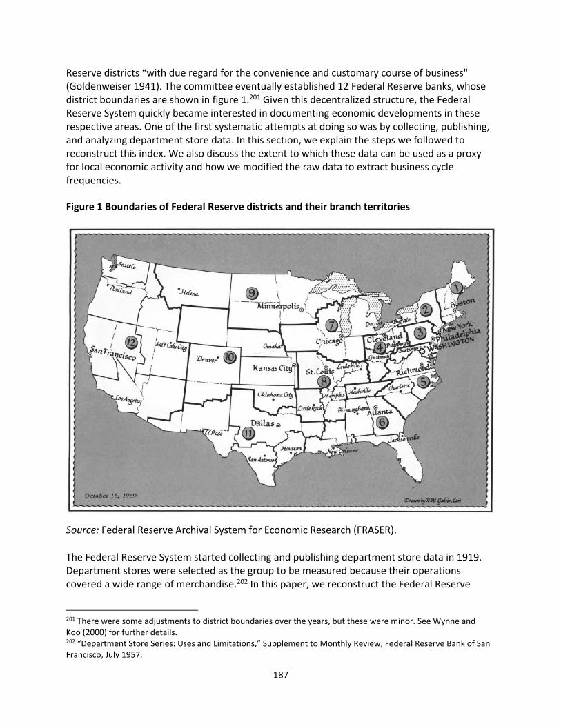
187  

Reserve districts “with due regard for the convenience and customary course of business" (Goldenweiser 1941). The committee eventually established 12 Federal Reserve banks, whose district boundaries are shown in figure 1.201 Given this decentralized structure, the Federal Reserve System quickly became interested in documenting economic developments in these respective areas. One of the first systematic attempts at doing so was by collecting, publishing, and analyzing department store data. In this section, we explain the steps we followed to reconstruct this index. We also discuss the extent to which these data can be used as a proxy for local economic activity and how we modified the raw data to extract business cycle frequencies.  

Figure 1 Boundaries of Federal Reserve districts and their branch territories 

 

Source: Federal Reserve Archival System for Economic Research (FRASER). 

The Federal Reserve System started collecting and publishing department store data in 1919. Department stores were selected as the group to be measured because their operations covered a wide range of merchandise.202 In this paper, we reconstruct the Federal Reserve 

                                                            201 There were some adjustments to district boundaries over the years, but these were minor. See Wynne and Koo (2000) for further details. 202 “Department Store Series: Uses and Limitations,” Supplement to Monthly Review, Federal Reserve Bank of San Francisco, July 1957.  

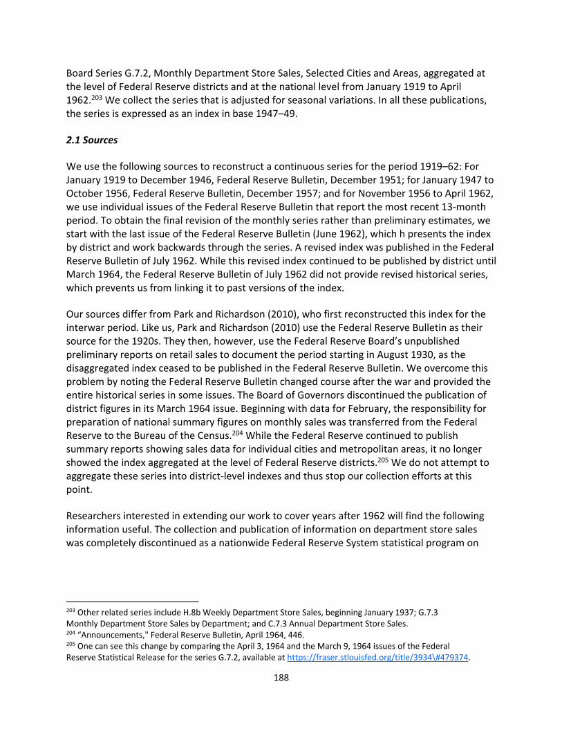
188  

Board Series G.7.2, Monthly Department Store Sales, Selected Cities and Areas, aggregated at the level of Federal Reserve districts and at the national level from January 1919 to April 1962.203 We collect the series that is adjusted for seasonal variations. In all these publications, the series is expressed as an index in base 1947–49.  

2.1 Sources  

We use the following sources to reconstruct a continuous series for the period 1919–62: For January 1919 to December 1946, Federal Reserve Bulletin, December 1951; for January 1947 to October 1956, Federal Reserve Bulletin, December 1957; and for November 1956 to April 1962, we use individual issues of the Federal Reserve Bulletin that report the most recent 13‐month period. To obtain the final revision of the monthly series rather than preliminary estimates, we start with the last issue of the Federal Reserve Bulletin (June 1962), which h presents the index by district and work backwards through the series. A revised index was published in the Federal Reserve Bulletin of July 1962. While this revised index continued to be published by district until March 1964, the Federal Reserve Bulletin of July 1962 did not provide revised historical series, which prevents us from linking it to past versions of the index.  

Our sources differ from Park and Richardson (2010), who first reconstructed this index for the interwar period. Like us, Park and Richardson (2010) use the Federal Reserve Bulletin as their source for the 1920s. They then, however, use the Federal Reserve Board’s unpublished preliminary reports on retail sales to document the period starting in August 1930, as the disaggregated index ceased to be published in the Federal Reserve Bulletin. We overcome this problem by noting the Federal Reserve Bulletin changed course after the war and provided the entire historical series in some issues. The Board of Governors discontinued the publication of district figures in its March 1964 issue. Beginning with data for February, the responsibility for preparation of national summary figures on monthly sales was transferred from the Federal Reserve to the Bureau of the Census.204 While the Federal Reserve continued to publish summary reports showing sales data for individual cities and metropolitan areas, it no longer showed the index aggregated at the level of Federal Reserve districts.205 We do not attempt to aggregate these series into district‐level indexes and thus stop our collection efforts at this point.  

Researchers interested in extending our work to cover years after 1962 will find the following information useful. The collection and publication of information on department store sales was completely discontinued as a nationwide Federal Reserve System statistical program on 

                                                            203 Other related series include H.8b Weekly Department Store Sales, beginning January 1937; G.7.3 Monthly Department Store Sales by Department; and C.7.3 Annual Department Store Sales. 204 “Announcements," Federal Reserve Bulletin, April 1964, 446. 205 One can see this change by comparing the April 3, 1964 and the March 9, 1964 issues of the Federal Reserve Statistical Release for the series G.7.2, available at https://fraser.stlouisfed.org/title/3934\#479374. 

189  

January 31, 1966.206 The first report in the monthly series measuring total sales of department stores in selected areas produced by the Bureau of the Census was published in April 1966 (BD, Special Current Business Reports, Monthly Department Store Sales in Selected Areas).207 In 1982, the data were reported in a new publication called BR, Current Business Reports, Monthly Retail Trade.208 The data then ceased to be published on paper in 1997 and became available online.209 

2.2 Description  

The Standard Industrial Classification Manual (Office of Statistical Standards 1941) defines department stores as “retail stores carrying a general line of apparel, such as suits, coats, dresses, and furnishings; home furnishings, such as furniture, floor coverings, curtains, draperies, linens, major household appliances, and housewares, such as table and kitchen appliances, dishes, and utensils." This definition became the standard definition used by the Federal Reserve System in assembling, classifying, and publishing statistical data for department stores.  

Table 1 Department store reporting samples, January 1962 

Federal Reserve district  Number of stores 

 

Percent ofvalue 

 

Boston (F.R. 1)   131   74  New York (F.R. 2)   165   80  Philadelphia (F.R. 3)   88   85  Cleveland (F.R. 4)   124   78  Richmond (F.R. 5)   139   80  Atlanta (F.R. 6)   135   81  Chicago (F.R. 7)   417   90  St. Louis (F.R. 8)   73   84  Minneapolis (F.R. 9)   109   88  Kansas City (F.R. 10)   121   77  Dallas (F.R. 11)   110   81  San Francisco (F.R. 12)   250   81  United States   1,862   82  

Source: Federal Reserve Bulletin, July 1962.  

The Federal Reserve System developed the Department Store Sales Index to study district and local business conditions. For this reason, the sample of reporting stores was considerably 

                                                            206 See Board of Governors of the Federal Reserve System, August 1965 Announcement, available at https://fraser.stlouisfed.org/scribd/?item_id=40738\&filepath=/files/docs/releases/c73/c73_19650810_g73_announcement.pdf&start_page=1 or Seldin (2016). 207 It can be obtained at https://catalog.hathitrust.org/Record/000637301. 208 It can be obtained at https://catalog.hathitrust.org/Record/002449623. 209 It can be found at www.census.gov/retail/mrts/mrtshist.html. 

190  

larger than would ordinarily be needed to measure changes in department store sales on a national basis (Federal Reserve Bulletin, June 1944). The reporting samples covered a varying number of department stores over the years. They included about 500 stores in the 1920s and 1930s and increased to about more than one‐third of the 4,051 department stores counted in the 1939 Census of Business. In terms of total sales, the 1,400 stores sampled accounted for 70 percent of total sales by department stores in that year (Moore 1961). The sample increased to 1,676 department stores in 1956, whose aggregate sales accounted for about 85 percent of all department stores in the country (Federal Reserve Bulletin, December 1957). Table 1 displays this information for each Federal Reserve district and for the United States as a whole for the last year in our sample, 1962.  

Figure 2 Total retail sales and department store sales, 1929–43 

 

Notes: Total retail sales: Department of Commerce index. Source: Federal Reserve Bulletin, June 1944.  

Department store sales constitute only approximately 10 percent of total retail sales, so it is 

natural to ask if the former is a good proxy for the latter. Figure 2 compares the movements in 

the two series between 1929 and 1943. Overall the movements are very similar, reflecting the 

fact that department stores carry a broad line of merchandise. At certain times, department 

store sales, however, diverge from total retail sales. The decline in overall retail sales was, for 

example, more pronounced than the decline in department store sales during the Great 

Depression. This is unsurprising because the index for department stores does not include 

items such as automobiles and building materials that experienced particularly big declines 

during these years (Federal Reserve Bulletin, June 1944). Conversely, in 1942 and 1943, when 

production of automobiles for civilians was discontinued and gasoline rationing was instituted, 

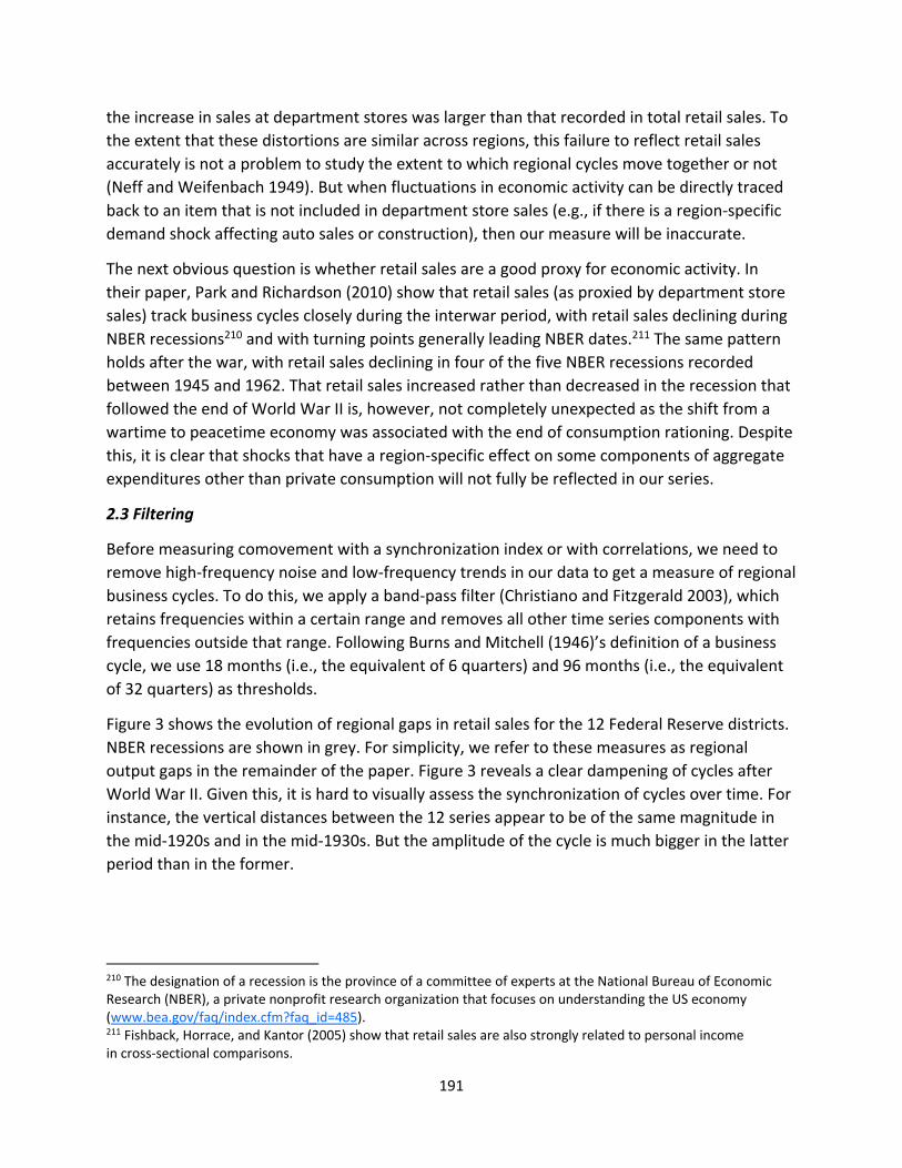
191  

the increase in sales at department stores was larger than that recorded in total retail sales. To 

the extent that these distortions are similar across regions, this failure to reflect retail sales 

accurately is not a problem to study the extent to which regional cycles move together or not 

(Neff and Weifenbach 1949). But when fluctuations in economic activity can be directly traced 

back to an item that is not included in department store sales (e.g., if there is a region‐specific 

demand shock affecting auto sales or construction), then our measure will be inaccurate.  

The next obvious question is whether retail sales are a good proxy for economic activity. In 

their paper, Park and Richardson (2010) show that retail sales (as proxied by department store 

sales) track business cycles closely during the interwar period, with retail sales declining during 

NBER recessions210 and with turning points generally leading NBER dates.211 The same pattern 

holds after the war, with retail sales declining in four of the five NBER recessions recorded 

between 1945 and 1962. That retail sales increased rather than decreased in the recession that 

followed the end of World War II is, however, not completely unexpected as the shift from a 

wartime to peacetime economy was associated with the end of consumption rationing. Despite 

this, it is clear that shocks that have a region‐specific effect on some components of aggregate 

expenditures other than private consumption will not fully be reflected in our series.  

2.3 Filtering  

Before measuring comovement with a synchronization index or with correlations, we need to 

remove high‐frequency noise and low‐frequency trends in our data to get a measure of regional 

business cycles. To do this, we apply a band‐pass filter (Christiano and Fitzgerald 2003), which 

retains frequencies within a certain range and removes all other time series components with 

frequencies outside that range. Following Burns and Mitchell (1946)’s definition of a business 

cycle, we use 18 months (i.e., the equivalent of 6 quarters) and 96 months (i.e., the equivalent 

of 32 quarters) as thresholds.  

Figure 3 shows the evolution of regional gaps in retail sales for the 12 Federal Reserve districts. 

NBER recessions are shown in grey. For simplicity, we refer to these measures as regional 

output gaps in the remainder of the paper. Figure 3 reveals a clear dampening of cycles after 

World War II. Given this, it is hard to visually assess the synchronization of cycles over time. For 

instance, the vertical distances between the 12 series appear to be of the same magnitude in 

the mid‐1920s and in the mid‐1930s. But the amplitude of the cycle is much bigger in the latter 

period than in the former. 

 

                                                            210 The designation of a recession is the province of a committee of experts at the National Bureau of Economic Research (NBER), a private nonprofit research organization that focuses on understanding the US economy (www.bea.gov/faq/index.cfm?faq_id=485). 211 Fishback, Horrace, and Kantor (2005) show that retail sales are also strongly related to personal income in cross‐sectional comparisons. 

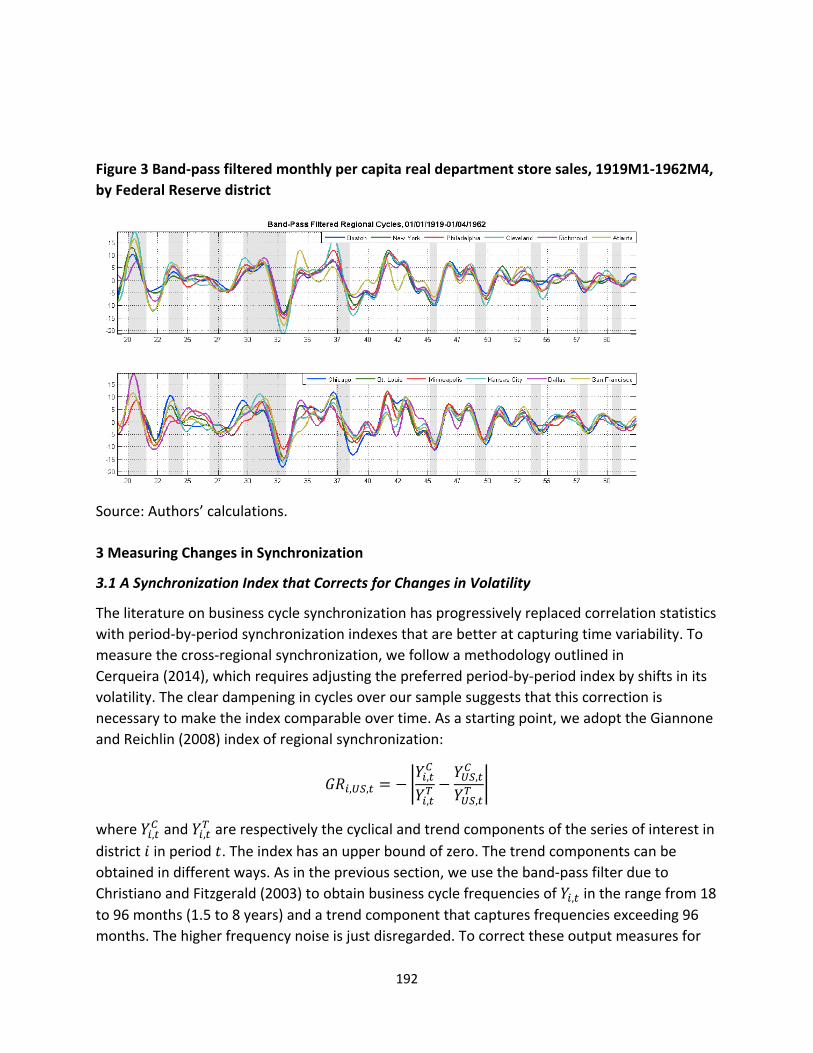
192  

 

 

Figure 3 Band‐pass filtered monthly per capita real department store sales, 1919M1‐1962M4, 

by Federal Reserve district 

   

Source: Authors’ calculations. 

 3 Measuring Changes in Synchronization 

3.1 A Synchronization Index that Corrects for Changes in Volatility 

The literature on business cycle synchronization has progressively replaced correlation statistics 

with period‐by‐period synchronization indexes that are better at capturing time variability. To 

measure the cross‐regional synchronization, we follow a methodology outlined in 

Cerqueira (2014), which requires adjusting the preferred period‐by‐period index by shifts in its 

volatility. The clear dampening in cycles over our sample suggests that this correction is 

necessary to make the index comparable over time. As a starting point, we adopt the Giannone 

and Reichlin (2008) index of regional synchronization:  

, ,,

,

,

, 

where  ,  and  ,  are respectively the cyclical and trend components of the series of interest in 

district   in period  . The index has an upper bound of zero. The trend components can be 

obtained in different ways. As in the previous section, we use the band‐pass filter due to 

Christiano and Fitzgerald (2003) to obtain business cycle frequencies of  ,  in the range from 18 

to 96 months (1.5 to 8 years) and a trend component that captures frequencies exceeding 96 

months. The higher frequency noise is just disregarded. To correct these output measures for 

193  

volatility changes, we first need to identify volatility shifts. For simplicity, we consider the 

following three subperiods: before the Great Depression; between the Great Depression and 

World War II; and after World War II.212 Equipped with these change points ( , we calculate 

the standard deviations of regional sales gaps for the respective subperiods and standardize the 

gaps  ,∗ . 

,,

, 

,∗ ,

, :

, , 1, … , , 1 

where   denotes an estimated change point and  3. The final index is thus  

, , ,∗

,∗  

This gives us 12‐district US observations for each month. We then estimate a single time series 

that characterizes the dynamics of changes in regional synchronization. Following 

Cerqueira (2014), we fit a local quadratic regression (local polynomial regression of degree 

two). Weights to neighboring observations are assigned according to the Epanechnikov kernel, 

and the width of the kernel (9 months) is determined based on generalized cross validation.  

Figure 4 shows the result. Several observations can be made from the figure. First, regional 

synchronization appears to increase during NBER recessions in our sample. Second, regional 

cycles were least synchronized in the mid‐1920s. Synchronization increased in the 1930s and 

has since remained high (that is, until the early 1960s). It is, however, difficult to get a sense 

from the graph of whether this increase of about 20 basis points in the index is big. To provide 

some metric, one can note that the cross‐country index calculated by Cerqueira (2014) for the 

period 1960 to the mid‐2010s ranges from –1.35 to –1.05. The author documents a first 

increase of 30 basis points in the 1960s. The index then progressively declines by 15 basis 

points until the mid‐1990s, at which point it again increases by about 15 basis points. Overall, 

this suggests that the increase in synchronization that we document is not negligible.  

 

 

 

                                                            212 An alternative approach to identify change points is to use an algorithm to detect change points in a time series. As robustness checks, we used the Segment Neighborhood approach (Auger and Lawrence 1989) using the Schwarz Information Criterion, with the number of change points being restricted to four. We applied the procedure to the aggregated index of US retail sales and applied the identified breaks to all districts. We also applied the procedure to identify district‐specific change points. In all cases, the pattern documented in figure 4 is unchanged.  

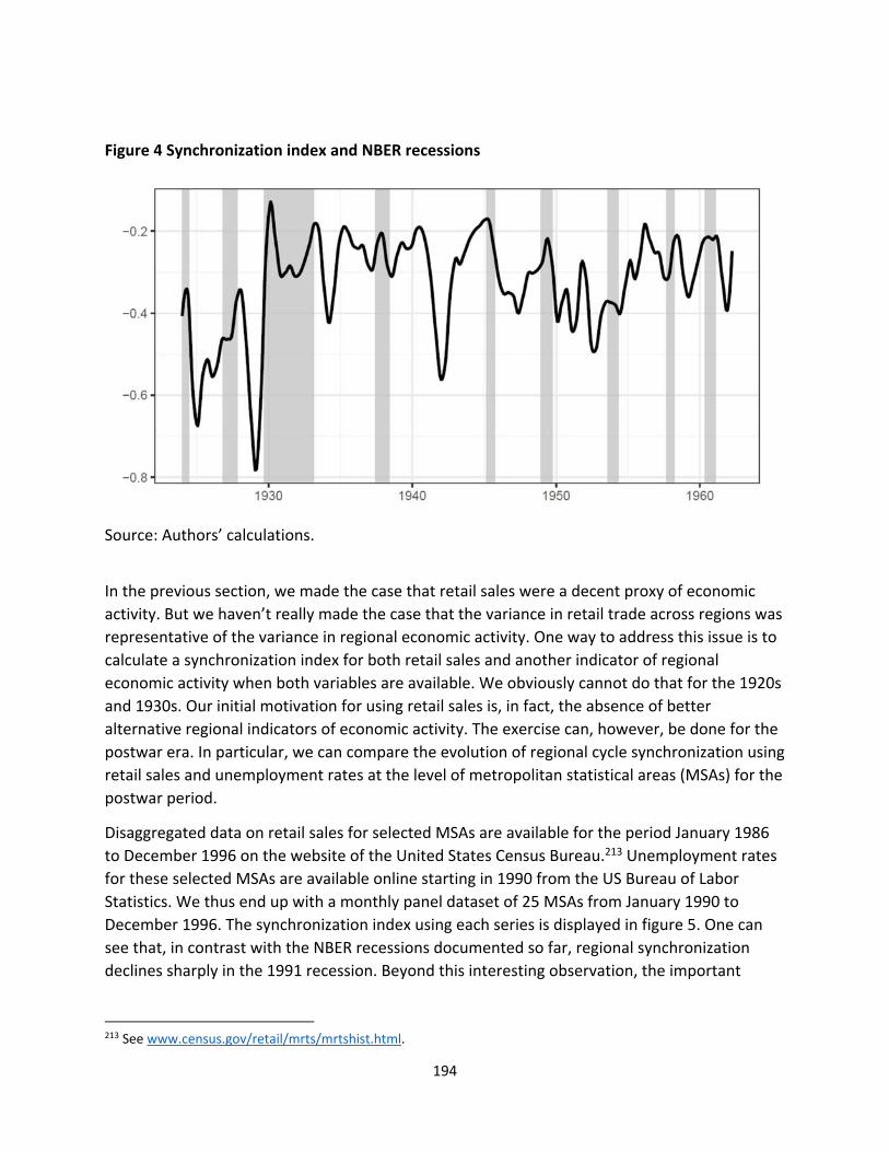
194  

 

Figure 4 Synchronization index and NBER recessions 

  

Source: Authors’ calculations.  

In the previous section, we made the case that retail sales were a decent proxy of economic 

activity. But we haven’t really made the case that the variance in retail trade across regions was 

representative of the variance in regional economic activity. One way to address this issue is to 

calculate a synchronization index for both retail sales and another indicator of regional 

economic activity when both variables are available. We obviously cannot do that for the 1920s 

and 1930s. Our initial motivation for using retail sales is, in fact, the absence of better 

alternative regional indicators of economic activity. The exercise can, however, be done for the 

postwar era. In particular, we can compare the evolution of regional cycle synchronization using 

retail sales and unemployment rates at the level of metropolitan statistical areas (MSAs) for the 

postwar period.  

Disaggregated data on retail sales for selected MSAs are available for the period January 1986 

to December 1996 on the website of the United States Census Bureau.213 Unemployment rates 

for these selected MSAs are available online starting in 1990 from the US Bureau of Labor 

Statistics. We thus end up with a monthly panel dataset of 25 MSAs from January 1990 to 

December 1996. The synchronization index using each series is displayed in figure 5. One can 

see that, in contrast with the NBER recessions documented so far, regional synchronization 

declines sharply in the 1991 recession. Beyond this interesting observation, the important 

                                                            213 See www.census.gov/retail/mrts/mrtshist.html. 

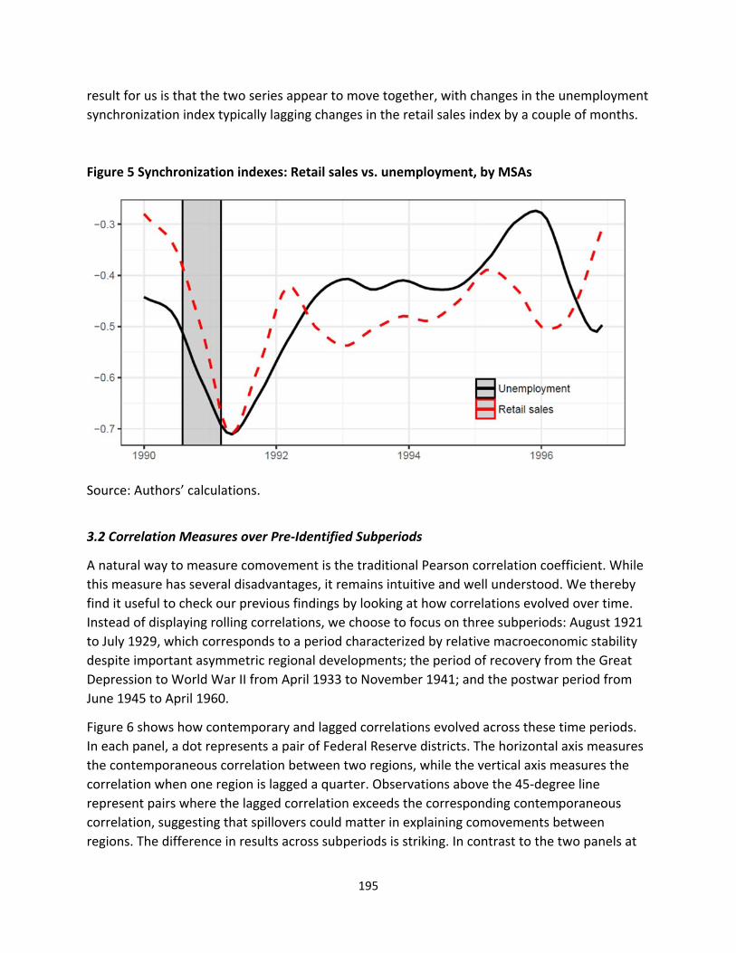
195  

result for us is that the two series appear to move together, with changes in the unemployment 

synchronization index typically lagging changes in the retail sales index by a couple of months.  

 

Figure 5 Synchronization indexes: Retail sales vs. unemployment, by MSAs 

 

Source: Authors’ calculations.  

3.2 Correlation Measures over Pre‐Identified Subperiods  

A natural way to measure comovement is the traditional Pearson correlation coefficient. While 

this measure has several disadvantages, it remains intuitive and well understood. We thereby 

find it useful to check our previous findings by looking at how correlations evolved over time. 

Instead of displaying rolling correlations, we choose to focus on three subperiods: August 1921 

to July 1929, which corresponds to a period characterized by relative macroeconomic stability 

despite important asymmetric regional developments; the period of recovery from the Great 

Depression to World War II from April 1933 to November 1941; and the postwar period from 

June 1945 to April 1960.  

Figure 6 shows how contemporary and lagged correlations evolved across these time periods. 

In each panel, a dot represents a pair of Federal Reserve districts. The horizontal axis measures 

the contemporaneous correlation between two regions, while the vertical axis measures the 

correlation when one region is lagged a quarter. Observations above the 45‐degree line 

represent pairs where the lagged correlation exceeds the corresponding contemporaneous 

correlation, suggesting that spillovers could matter in explaining comovements between 

regions. The difference in results across subperiods is striking. In contrast to the two panels at 

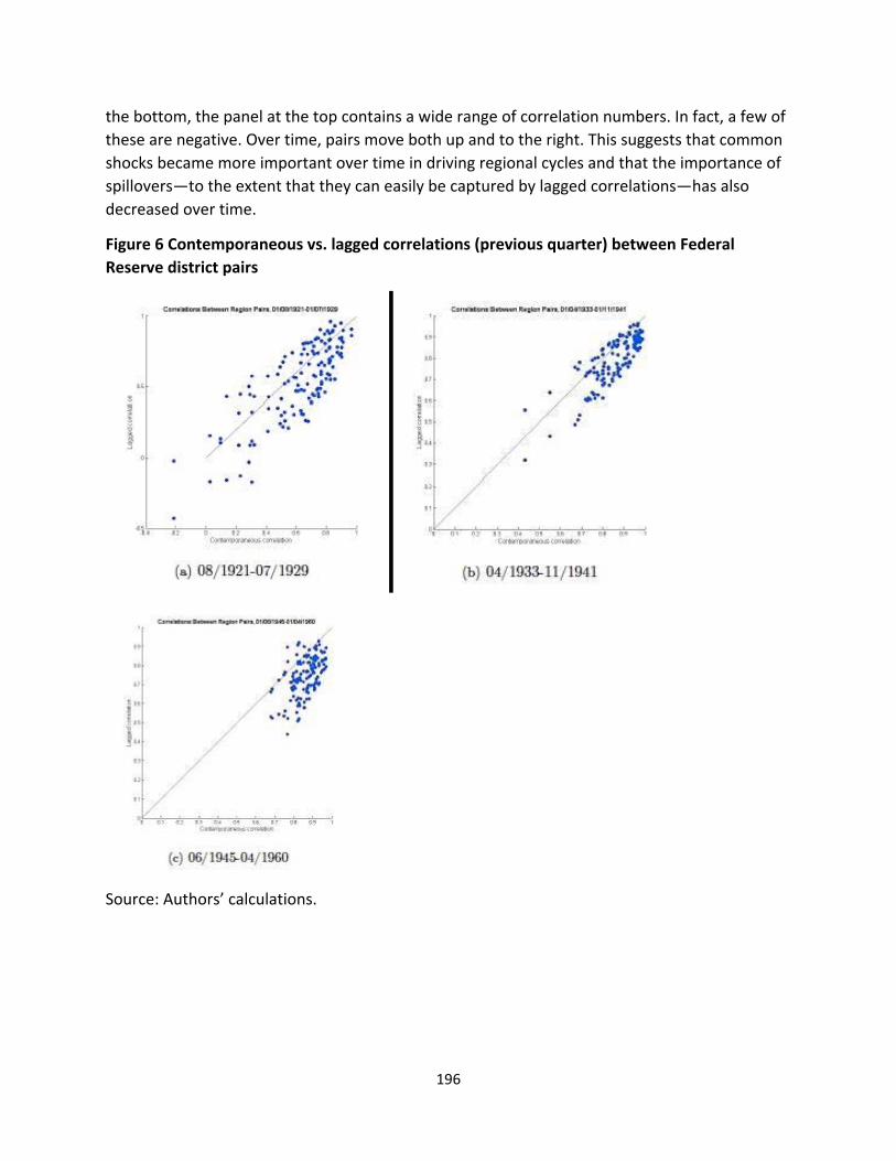
196  

the bottom, the panel at the top contains a wide range of correlation numbers. In fact, a few of 

these are negative. Over time, pairs move both up and to the right. This suggests that common 

shocks became more important over time in driving regional cycles and that the importance of 

spillovers—to the extent that they can easily be captured by lagged correlations—has also 

decreased over time.  

Figure 6 Contemporaneous vs. lagged correlations (previous quarter) between Federal 

Reserve district pairs 

   

 

Source: Authors’ calculations. 

    

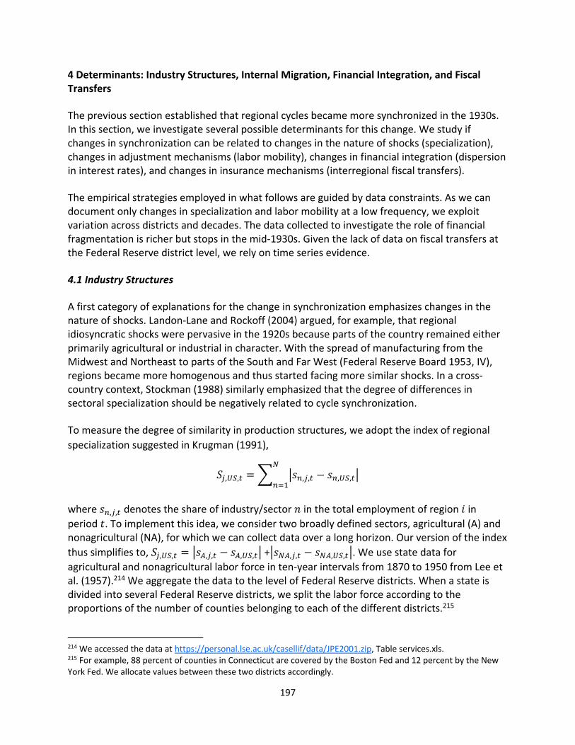
197  

4 Determinants: Industry Structures, Internal Migration, Financial Integration, and Fiscal Transfers 

The previous section established that regional cycles became more synchronized in the 1930s. In this section, we investigate several possible determinants for this change. We study if changes in synchronization can be related to changes in the nature of shocks (specialization), changes in adjustment mechanisms (labor mobility), changes in financial integration (dispersion in interest rates), and changes in insurance mechanisms (interregional fiscal transfers).  

The empirical strategies employed in what follows are guided by data constraints. As we can document only changes in specialization and labor mobility at a low frequency, we exploit variation across districts and decades. The data collected to investigate the role of financial fragmentation is richer but stops in the mid‐1930s. Given the lack of data on fiscal transfers at the Federal Reserve district level, we rely on time series evidence.   

4.1 Industry Structures 

A first category of explanations for the change in synchronization emphasizes changes in the nature of shocks. Landon‐Lane and Rockoff (2004) argued, for example, that regional idiosyncratic shocks were pervasive in the 1920s because parts of the country remained either primarily agricultural or industrial in character. With the spread of manufacturing from the Midwest and Northeast to parts of the South and Far West (Federal Reserve Board 1953, IV), regions became more homogenous and thus started facing more similar shocks. In a cross‐country context, Stockman (1988) similarly emphasized that the degree of differences in sectoral specialization should be negatively related to cycle synchronization.  

To measure the degree of similarity in production structures, we adopt the index of regional 

specialization suggested in Krugman (1991), 

, , , , , ,  

where  , ,  denotes the share of industry/sector   in the total employment of region   in 

period  . To implement this idea, we consider two broadly defined sectors, agricultural (A) and nonagricultural (NA), for which we can collect data over a long horizon. Our version of the index 

thus simplifies to,  , , , , , ,  + , , , , . We use state data for 

agricultural and nonagricultural labor force in ten‐year intervals from 1870 to 1950 from Lee et al. (1957).214 We aggregate the data to the level of Federal Reserve districts. When a state is divided into several Federal Reserve districts, we split the labor force according to the proportions of the number of counties belonging to each of the different districts.215 

                                                            214 We accessed the data at https://personal.lse.ac.uk/casellif/data/JPE2001.zip, Table services.xls. 215 For example, 88 percent of counties in Connecticut are covered by the Boston Fed and 12 percent by the New York Fed. We allocate values between these two districts accordingly. 

198  

Figure 7 Specialization indexes 

 

Source: Authors’ calculations. 

Figure 7 displays these measures and shows the progressive convergence in industry structures. All districts, except Minneapolis and Kansas City, see their specialization come closer to that of the United States as whole. A Federal Reserve study in the early 1950s (Federal Reserve Board 1953, 12–13) illustrates this finding clearly: “The growing diversification that has taken place within all Federal Reserve districts over the past two decades makes it difficult to classify very many districts any longer as primarily agricultural in character.”216 The rates of convergence, however, vary across districts, suggesting that some of that variation might be used to identify the impact of diversification on synchronization.  

In figure 8, we thus look directly at the relationship between diversification and synchronization. On the horizontal axis, we plot the specialization index at the beginning of the decade. On the vertical axis, we plot the average of the synchronization index over that same decade. The labels indicate the Federal Reserve district behind the observation. While the raw data suggest a negative relationship (that is, in fact, statistically significant at the 10 percent level) between specialization and synchronization, it is easy to see that the relationship is nonrobust (both to time fixed effects and district fixed effects). In fact, for most districts, a higher level of synchronization is not necessarily associated with a higher level of synchronization. This reflects the fact that for most districts, the jump in synchronization happens between the 1920s and the 1930s while the increase in diversification is continuous and gains steam, especially after the 1930s.  

                                                            216 The report then notes that this “growing diversification [...] has tended to remove the basis for [discount rate] differentials which existed when System policy could effectively distinguish between the predominantly agricultural and the predominantly industrial sections of the country." 

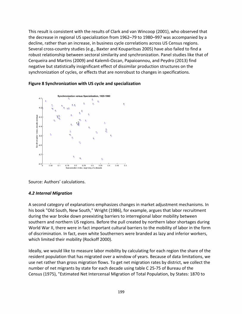
199  

This result is consistent with the results of Clark and van Wincoop (2001), who observed that the decrease in regional US specialization from 1962–79 to 1980–997 was accompanied by a decline, rather than an increase, in business cycle correlations across US Census regions. Several cross‐country studies (e.g., Baxter and Kouparitsas 2005) have also failed to find a robust relationship between sectoral similarity and synchronization. Panel studies like that of Cerqueira and Martins (2009) and Kalemli‐Ozcan, Papaioannou, and Peydro (2013) find negative but statistically insignificant effect of dissimilar production structures on the synchronization of cycles, or effects that are nonrobust to changes in specifications.  

Figure 8 Synchronization with US cycle and specialization 

 

Source: Authors’ calculations. 

4.2 Internal Migration 

A second category of explanations emphasizes changes in market adjustment mechanisms. In his book "Old South, New South," Wright (1986), for example, argues that labor recruitment during the war broke down preexisting barriers to interregional labor mobility between southern and northern US regions. Before the pull created by northern labor shortages during World War II, there were in fact important cultural barriers to the mobility of labor in the form of discrimination. In fact, even white Southerners were branded as lazy and inferior workers, which limited their mobility (Rockoff 2000).  

Ideally, we would like to measure labor mobility by calculating for each region the share of the resident population that has migrated over a window of years. Because of data limitations, we use net rather than gross migration flows. To get net migration rates by district, we collect the number of net migrants by state for each decade using table C 25‐75 of Bureau of the Census (1975), "Estimated Net Intercensal Migration of Total Population, by States: 1870 to 

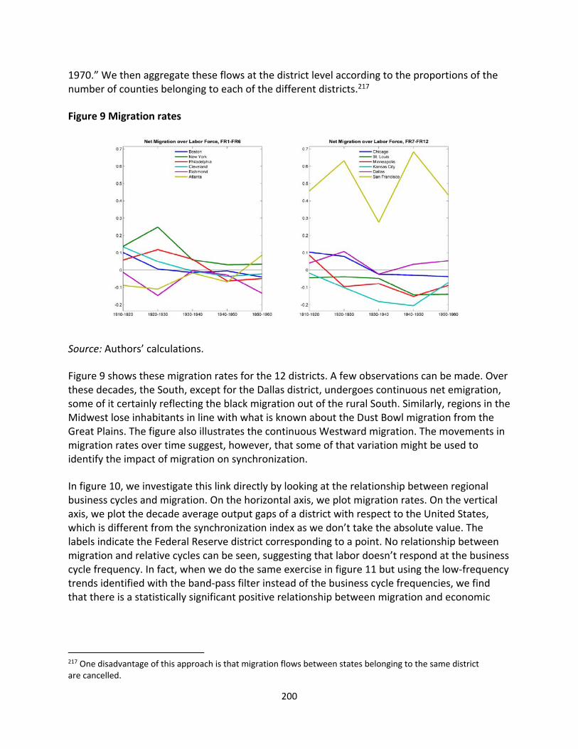
200  

1970.” We then aggregate these flows at the district level according to the proportions of the number of counties belonging to each of the different districts.217 

Figure 9 Migration rates 

 

Source: Authors’ calculations. 

Figure 9 shows these migration rates for the 12 districts. A few observations can be made. Over these decades, the South, except for the Dallas district, undergoes continuous net emigration, some of it certainly reflecting the black migration out of the rural South. Similarly, regions in the Midwest lose inhabitants in line with what is known about the Dust Bowl migration from the Great Plains. The figure also illustrates the continuous Westward migration. The movements in migration rates over time suggest, however, that some of that variation might be used to identify the impact of migration on synchronization.  

In figure 10, we investigate this link directly by looking at the relationship between regional business cycles and migration. On the horizontal axis, we plot migration rates. On the vertical axis, we plot the decade average output gaps of a district with respect to the United States, which is different from the synchronization index as we don’t take the absolute value. The labels indicate the Federal Reserve district corresponding to a point. No relationship between migration and relative cycles can be seen, suggesting that labor doesn’t respond at the business cycle frequency. In fact, when we do the same exercise in figure 11 but using the low‐frequency trends identified with the band‐pass filter instead of the business cycle frequencies, we find that there is a statistically significant positive relationship between migration and economic 

                                                            217 One disadvantage of this approach is that migration flows between states belonging to the same district are cancelled. 

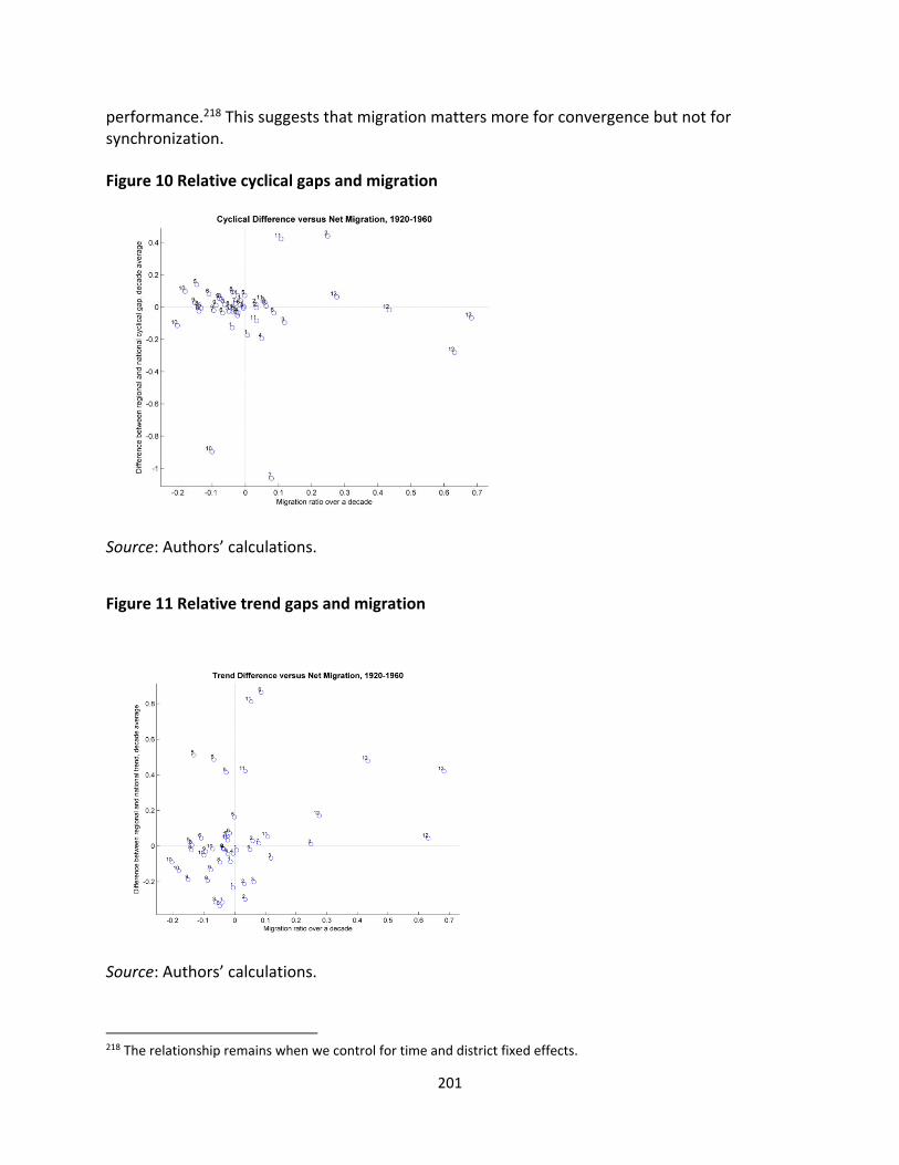
201  

performance.218 This suggests that migration matters more for convergence but not for synchronization.  

Figure 10 Relative cyclical gaps and migration 

 

Source: Authors’ calculations.  

Figure 11 Relative trend gaps and migration 

 

 

Source: Authors’ calculations.  

                                                            218 The relationship remains when we control for time and district fixed effects. 

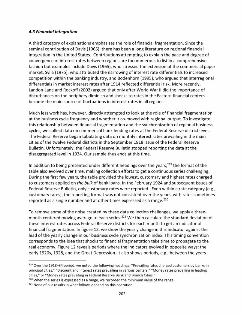
202  

4.3 Financial Integration 

A third category of explanations emphasizes the role of financial fragmentation. Since the seminal contribution of Davis (1965), there has been a long literature on regional financial integration in the United States.  Contributions attempting to explain the pace and degree of convergence of interest rates between regions are too numerous to list in a comprehensive fashion but examples include Davis (1965), who stressed the extension of the commercial paper market, Sylla (1975), who attributed the narrowing of interest rate differentials to increased competition within the banking industry, and Bodenhorn (1995), who argued that interregional differentials in market interest rates after 1914 reflected differential risk. More recently, Landon‐Lane and Rockoff (2002) argued that only after World War II did the importance of disturbances on the periphery diminish and shocks to rates in the Eastern financial centers became the main source of fluctuations in interest rates in all regions. 

Much less work has, however, directly attempted to look at the role of financial fragmentation at the business cycle frequency and whether it co‐moved with regional output. To investigate this relationship between financial fragmentation and the synchronization of regional business cycles, we collect data on commercial bank lending rates at the Federal Reserve district level. The Federal Reserve began tabulating data on monthly interest rates prevailing in the main cities of the twelve Federal districts in the September 1918 issue of the Federal Reserve Bulletin. Unfortunately, the Federal Reserve Bulletin stopped reporting the data at the disaggregated level in 1934. Our sample thus ends at this time.  

In addition to being presented under different headings over the years,219 the format of the table also evolved over time, making collection efforts to get a continuous series challenging. During the first few years, the table provided the lowest, customary and highest rates charged to customers applied on the bulk of bank loans. In the February 1924 and subsequent issues of Federal Reserve Bulletin, only customary rates were reported.  Even within a rate category (e.g., customary rates), the reporting format was not consistent over the years, with rates sometimes reported as a single number and at other times expressed as a range.220  

To remove some of the noise created by these data collection challenges, we apply a three‐month centered moving average to each series.221 We then calculate the standard deviation of these interest rates across Federal Reserve districts for each month to get an indicator of financial fragmentation. In figure 12, we show the yearly change in this indicator against the lead of the yearly change in our business cycle synchronization index. This timing convention corresponds to the idea that shocks to financial fragmentation take time to propagate to the real economy. Figure 12 reveals periods where the indicators evolved in opposite ways: the early 1920s, 1928, and the Great Depression. It also shows periods, e.g., between the years 

                                                            219 Over the 1918–34 period, we noted the following headings: “Prevailing rates charged customers by banks in principal cities,” “Discount and interest rates prevailing in various centers,” “Money rates prevailing in leading cities," or “Money rates prevailing in Federal Reserve Bank and Branch Cities.” 220 When the series is expressed as a range, we recorded the minimum value of the range. 221 None of our results in what follows depend on this operation. 

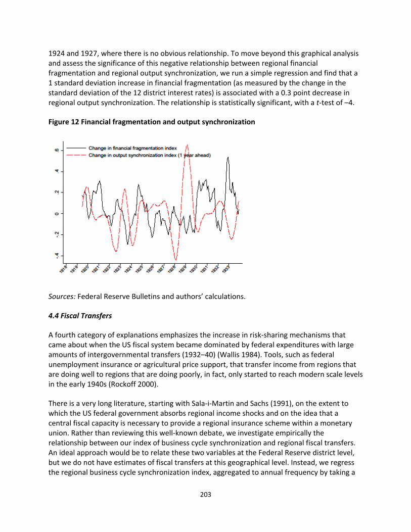
203  

1924 and 1927, where there is no obvious relationship. To move beyond this graphical analysis and assess the significance of this negative relationship between regional financial fragmentation and regional output synchronization, we run a simple regression and find that a 1 standard deviation increase in financial fragmentation (as measured by the change in the standard deviation of the 12 district interest rates) is associated with a 0.3 point decrease in regional output synchronization. The relationship is statistically significant, with a t‐test of –4. 

Figure 12 Financial fragmentation and output synchronization 

 

Sources: Federal Reserve Bulletins and authors’ calculations. 

4.4 Fiscal Transfers 

A fourth category of explanations emphasizes the increase in risk‐sharing mechanisms that came about when the US fiscal system became dominated by federal expenditures with large amounts of intergovernmental transfers (1932–40) (Wallis 1984). Tools, such as federal unemployment insurance or agricultural price support, that transfer income from regions that are doing well to regions that are doing poorly, in fact, only started to reach modern scale levels in the early 1940s (Rockoff 2000).  

There is a very long literature, starting with Sala‐i‐Martin and Sachs (1991), on the extent to which the US federal government absorbs regional income shocks and on the idea that a central fiscal capacity is necessary to provide a regional insurance scheme within a monetary union. Rather than reviewing this well‐known debate, we investigate empirically the relationship between our index of business cycle synchronization and regional fiscal transfers. An ideal approach would be to relate these two variables at the Federal Reserve district level, but we do not have estimates of fiscal transfers at this geographical level. Instead, we regress the regional business cycle synchronization index, aggregated to annual frequency by taking a 

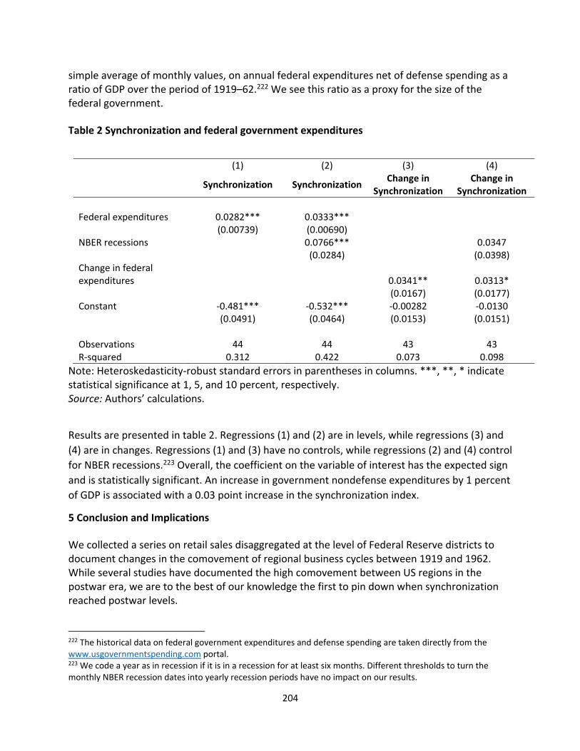
204  

simple average of monthly values, on annual federal expenditures net of defense spending as a ratio of GDP over the period of 1919–62.222 We see this ratio as a proxy for the size of the federal government.  

Table 2 Synchronization and federal government expenditures 

              

   (1)  (2)  (3)  (4) 

  Synchronization  Synchronization 

Change in Synchronization 

Change in Synchronization 

              Federal expenditures  0.0282***  0.0333***          (0.00739)  (0.00690)       NBER recessions     0.0766***     0.0347       (0.0284)     (0.0398) Change in federal expenditures        0.0341**  0.0313*          (0.0167)  (0.0177) Constant  ‐0.481***  ‐0.532***  ‐0.00282  ‐0.0130    (0.0491)  (0.0464)  (0.0153)  (0.0151)               Observations  44  44  43  43 R‐squared  0.312  0.422  0.073  0.098 

Note: Heteroskedasticity‐robust standard errors in parentheses in columns. ***, **, * indicate statistical significance at 1, 5, and 10 percent, respectively. Source: Authors’ calculations.  

Results are presented in table 2. Regressions (1) and (2) are in levels, while regressions (3) and 

(4) are in changes. Regressions (1) and (3) have no controls, while regressions (2) and (4) control 

for NBER recessions.223 Overall, the coefficient on the variable of interest has the expected sign 

and is statistically significant. An increase in government nondefense expenditures by 1 percent 

of GDP is associated with a 0.03 point increase in the synchronization index.  

5 Conclusion and Implications 

We collected a series on retail sales disaggregated at the level of Federal Reserve districts to document changes in the comovement of regional business cycles between 1919 and 1962. While several studies have documented the high comovement between US regions in the postwar era, we are to the best of our knowledge the first to pin down when synchronization reached postwar levels.  

                                                            222 The historical data on federal government expenditures and defense spending are taken directly from the www.usgovernmentspending.com portal. 223 We code a year as in recession if it is in a recession for at least six months. Different thresholds to turn the monthly NBER recession dates into yearly recession periods have no impact on our results.  

205  

We find that regional economic cycle synchronization increased substantially in the 1930s and has since remained high. Using data on regional industry structures, we find that the industrialization of agricultural regions and changes in the responsiveness of migration flows to asymmetric shocks fail to explain the increase in the synchronization of regional cycles. We, however, find a strong relationship with changes in regional financial fragmentation and with the increase in interregional fiscal transfers.  

This suggests that the reduced divergence in regional financial conditions and the creation of a 

federal fiscal capacity were instrumental in dampening the importance of region‐specific shocks 

in the United States. In the European context, completion of the banking union and creation of 

new credit facilities for countries that lose market access (e.g., through the European Stability 

Mechanism) would help dampen the importance of regional shocks to financial conditions, while 

the possibility to activate resources rapidly from a common budget (e.g.,  through a European 

insurance or an investment stabilization program) would provide buffers against shocks that do 

not necessarily emanate from the financial sector.  

References 

Auger, Ivan E., and Charles E. Lawrence. 1989. Algorithms for the optimal identification of segment neighborhoods. Bulletin of Mathematical Biology 51, no. 1: 39–54.   Baxter, Marianne and Michael A. Kouparitsas. 2005. Determinants of business cycle comovement: A robust analysis. Journal of Monetary Economics 52, no. 1 (January): 113–57.   Bayoumi, Tamim, and Barry Eichengreen. 1992. Shocking Aspects of European Monetary Unification. NBER Working Paper 3949. Cambridge, MA: National Bureau of Economic Research.   Bayoumi, Tamim, and Barry Eichengreen. 2017. Aftershocks of Monetary Unification: Hysteresis with a Financial Twist. NBER Working Paper 23205 (February). Cambridge, MA: National Bureau of Economic Research.   Bodenhorn, Howard. 1995. A More Perfect Union: Regional Interest Rates in the United States, 1880–1960. In Anglo‐American Financial Systems: Institutions and Markets in the Twentieth Century, ed. Michael D. Bordo and Richard Sylla. Irwin Professional Pub.  Bordo, M. D., C. Goldin, and E. N. White. 2007. The Defining Moment: The Great Depression and the American Economy in the Twentieth Century. National Bureau of Economic Research Project Report. Chicago: University of Chicago Press.   Bureau of the Census. 1975. Historical Statistics of the United States, Colonial Times to 1970. Bicentennial Edition, Part 1. Washington: US Department of Commerce.   Burns, Arthur F., and Wesley C. Mitchell. 1946. Measuring Business Cycles. Cambridge, MA: National Bureau of Economic Research.  

206  

 Campos, Nauro F., and Corrado Macchiarelli. 2016. Core and Periphery in the European Monetary Union: Bayoumi and Eichengreen 25 Years Later. Economics Letters 147 (October): 127–30.   Carlino, Gerald A., and Keith Sill. 1998. The Cyclical Behavior of Regional Per Capita Incomes in the Postwar Period. Working Paper 98‐11. Federal Reserve Bank of Philadelphia.   Cerqueira, Pedro André. 2014. Business Cycle Synchronization and Volatility Shifts. GEMF Working Paper 2014‐19 (September). Portugal: GEMF and Faculty of Economics, University of Coimbra.   Cerqueira, Pedro André, and Rodrigo Martins. 2009. Measuring the determinants of business cycle synchronization using a panel approach. Economics Letters 102, no. 2 (February): 106–108.   Christiano, Lawrence J., and Terry J. Fitzgerald. 2003. The Band Pass Filter. International Economic Review 44, no. 2: 435–65.   Clark, Todd E., and Eric van Wincoop. 2001. Borders and Business Cycles. Journal of International Economics 55, no. 1 (October): 59–85.   Davis, Lance E. 1965. The Investment Market, 1870‐1914: The Evolution of a National Market. Journal of Economic History 25, no. 3: 355–99.  Fishback, Price V., William C. Horrace, and Shawn Kantor. 2005. Did New Deal Grant Programs Stimulate Local Economies? A Study of Federal Grants and Retail Sales during the Great Depression. Journal of Economic History 65, no. 1: 36–71.   Federal Reserve Board. 1953. Discount and Discount Rate Mechanism: A Group of Special Studies (May). Board of Governors of the Federal Reserve System. Available at https://fraser.stlouisfed.org/title/?id=3967.   Frankel, Jeffrey A., and Andrew K. Rose. 1996. The Endogeneity of the Optimum Currency Area Criteria. NBER Working Paper 5700 (August). Cambridge, MA: National Bureau of Economic Research.   Giannone, Domenico, and Lucrezia Reichlin. 2008. Did the euro imply more correlation of cycles? Technical Report. Universite Libre de Bruxelles.  Goldenweiser, Emmanuel A. 1941. Public Nature of the Reserve Banks. Board of Governors of the Federal Reserve System.   

207  

Imbs, Jean. 2004. Trade, Finance, Specialization, and Synchronization. Review of Economics and Statistics 86, no. 3: 723–34.   Kalemli‐Ozcan, Sebnem, Elias Papaioannou, and José‐Luis Peydro. 2013. Financial Regulation, Financial Globalization, and the Synchronization of Economic Activity. Journal of Finance 68, no. 3: 1179–228.   Kouparitsas, Michael A. 2002. Understanding U.S. regional cyclical comovement: How important are spillovers and common shocks? Economic Perspectives (4th Quarter): 30–41.   Krugman, Paul. 1991. Geography and Trade. MIT Press.   Landon‐Lane, John, and Hugh Rockoff. 2004. Monetary Policy and Regional Interest Rates in the United States, 1880‐2002. NBER Working Paper 10924 (November). Cambridge, MA: National Bureau of Economic Research.   Lee, Everett S., Ann Ratner Miller, Carol P. Brainerd, and Richard A. Easterlin. 1957. Population Redistribution and Economic Growth, United States, 1870–1950, Volume 1: Methodological Considerations and Reference Tables. American Philosophical Society.   Moore, Geoffrey H. ed. 1961. Business Cycle Indicators, Volume 2, Basic Data on Cyclical Indicators. Princeton University Press.  Mundell, Robert. 1961. A Theory of Optimum Currency Areas. American Economic Review 51, no. 4: 657–65.   Neff, P. and A. Weifenbach. 1949. Business Cycles in Selected Industrial Areas. John Randolph Haynes and Dora Haynes Foundation.  Office of Statistical Standards. 1941. Standard Industrial Classification Manual. Washington: Government Printing Office.  Park, Haelim M., and Gary Richardson. 2010. Retail Trade by Federal Reserve District, 1919 to 1939: A Statistical History. Working Paper 16617 (December). Cambridge, MA: National Bureau of Economic Research.   Rockoff, Hugh. 2000. How Long Did it Take the United States to Become an Optimal Currency Area? Working Paper 124 (April). Cambridge, MA: National Bureau of Economic Research.   Sala‐i‐Martin, Xavier, and Jeffrey Sachs. 1991. Fiscal Federalism and Optimum Currency Areas: Evidence for Europe From the United States. NBER Working Paper 3855 (October). Cambridge, MA: National Bureau of Economic Research.   

208  

Seldin, Sian L. 2016. Federal Reserve Board Statistical Releases: A Publications History. Finance and Economics Discussion Series 2016‐16 (March). Board of Governors of the Federal Reserve System.  Stockman, Alan C. 1988. Sectoral and national aggregate disturbances to industrial output in seven European countries. Journal of Monetary Economics 21, no. 2‐3: 387–409.   Sylla, R. E. 1975. The American Capital Market, 1846‐1914: A study of the effects of public policy on economic development. Dissertations in American economic history. Arno Press.  Wallis, John Joseph. 1984. The Birth of the Old Federalism: Financing the New Deal, 1932–1940. Journal of Economic History 44, no. 01: 139–59.   Wright, G. 1986. Old South, New South: Revolutions in the Southern Economy Since the Civil War. Basic Books.   Wynne, Mark A. and Jahyeong Koo. 2000. Business Cycles under Monetary Union: A Comparison of the EU and US. Economica 67, no. 267 (August): 347–74.