REPORT II GROUP 1 - NASA · frequency, a dxer amplifier, a transmitter, and a paver amplifier used for transmitting signals from space vehicle to a ground receiving station. 8 1 -

MARVIN A. GRlFFIN RICHARD S. SfMPSON

Project Directors

I H. PAUL HASSELL, JR.

Research Astociote

1 GPO

CFST

Jma, 1%

1 TECMNtCU REPORT NUMBER 13 I!

h

ff 853 July 65

II SYSTEMS ENGINEERING GROUP

BUREAU OF ENGINEERING RESEARCH

UNIVERSITY OF ALABAMA UNIVERSITY, ALABAMA

1

n

https://ntrs.nasa.gov/search.jsp?R=19660025348 2020-07-26T02:43:31+00:00Z

I - t !

1 I I I I I

STATISTICAL QUALITY CONTROL

APPLIED TO A TELEMETRY SYSTEM

ACCEPTANCE PROCEDURE

Marvin A. Griffin Richard S. Simpson Project Directors

H . Paul Hassell, Jr. Research Associate

W i l l i a m S . Spivey Graduate Assistant

June, 1966

TECHNICAL REPORT NUMBER 13

Prepared for

National Aeronautics and Space Administration Marshall Space Flight Center

Huntsville, Alabama

Under

CONTRACT NUMBER NAS8-20172

Systems Engineering Group Bureau of Engineering Research

University of Alabama

ABSTRACT

This is the thir teenth of a series of technical repor t s concerned

with the Te leme t ry Systems on t h e Saturn vehicle.

The purpose of t h i s report is t o develop a methodology f o r

implementing s ta t is t ical control char t s as a bas i s fo r telemetry

package acceptance procedures.

the control char t f o r mean values and f o r t he control char t fo r

standard deviations.

The methodology is developed for both

A t o t a l expected cost model which relates alpha and beta e r ro r s

as w e l l as the sample s ize is developed. This model is used t o

es tab l i sh optimum upper and lower control l i m i t s f o r the chart f o r

mean values. Control limits for t he chart f o r standard deviations

are then established based on t h i s model.

An experiment t ha t w a s designed and conducted f o r t he purpose

of t es t ing the f e a s i b i l i t y of t h e optimum control l i m i t s is reported.

Results of t h i s experiment confirm the reasonableness of the assumptions

made in the cost model. Subcarrier o sc i l l a to r s i n the experimental

telemetry package tha t w e r e in tent ional ly maladjusted are detected

by the control charts.

E s t i m a t e s of the accuracy and precision of the telemetry

package are obtained and ninety-nine per cent confidence l i m i t s are

established fo r these l i m i t s .

Standards for future control chart analysis are established fo r

both charts . These standards may be used for future package

checkout procedures.

I I - 8 I 1 I t I t 1 1 t I I 1 8 I 1 I

TABLE OF CONTENTS

Page

ABSTRACT . . . . . . . . . . . . . . . . . . . . . . . . . . . . if

LISTOFTABLES e . 0 0 . . 0 . . V

. . . . . . . . . . . . . . . . . . . . LISTOF ILLUSTRATIONS. vi

Chapter I. INTRODUCTION . . . . . . . . . . . . . . . . . . . . . . 1

Statement of the Problem The Proposed Methodology

. . . . . . . . . 11, THE GENERAL THEORY OF CONTROL CHARTS 8

111. THE DEVELOPMENT OF THE METHODOLOGY . . . . . . . . . . 14

The X-Chart The u-Chart Estimation of uc Effects of Non-Normality Swmtary of the Methodology

IV. THE DEVELOPMENT OF THE PROBABILITY FUNCTIONS FOR THE TYPE I AND TYPE I1 ERRORS . . . . . . . . . . 37

Operating - Characteristic Function for the

Operating Characteristic Function for the

Probability Function for a for the %Chart Probability Function for a for the u-Chart

X-Chart

a-Chart

V. THE DETERMINATION OF THE PROPER LIMIT CONSTANT . . . . 47

VI. APPLICATION OF THE METHowLoGy . . . . . . . . . . . . 55

Description of the Experimental Output Determination of the Optimum K and n Analysis by Control Charts

iii

Chapter

S-rY Sources of Poss ib le Error Reconmendations for Future Research and Application

Page

APPENDICES . . . . . 0 85

A. Miscellaneous Proofs, Theorems, and Sample Calculations . . . . . . . . . . . . . . . . 86

B. Glossary of Symbols . . . . . . . . . . . . . . . . . 93

LISTOFREFERENCES 0 . . 0 . . . . 97

BIBLIOGRAPHY . . . . . . . . . . . . . . . . . . . . . . . . . 100

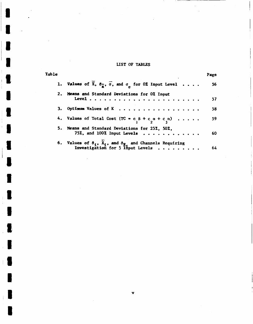
LIST OF TABLES

Table Page - . . . . 1. Values of E, O--, u, and u for 0% Input Level 56

2. L e v e l . . . . . . . . . . . . . . . . . . . . . . . 57

0

?kans and Standard Deviations for 0% Input

3. Optimum Values of K . . . . . . . . . . . . . . . . . 58

. . . . . 4. Values of Total Cost (TC = c 8 + c a + c n)

5. Means and Standard Deviations for 25X, SOX,

6. Values of 01, q, and U j z and Channels Requiring

59 1 2 3

75%, and 100% Input Levels . . . . . . . . . . . . 60

Investigation for 5 IAput Levels . . . . . . . . . 64

V

Figure

LIST OF ILLUSTRATIONS

Page

1. Distribution of Chance Variations i n a Sample MeasureofQuality . . . . . . . . . . . . . . .

2, I l l u s t r a t ion of the Theoretical B a s i s f o r a Cont ro lchar t . . . . . . . . . . . . - . .

3. Control Chart fo r 51 for Shoulder Depth of Fragmentation B d s . . . . . . . . . . . . . .

4. Control Chart fo r u fo r Shoulder Depth of FragmentationBombs . . . . . . . . . . . . . . . .

5. Block Diagram of the FM/FM Experimental Telemetry System . . . . . . . . . . . . . . .

6. Graph of f ( F ) Depicting Areas Under the Curve . . . 7. Control Chart f o r man Values of SCO's . . . . . . . i j

8. Control Chart for Standard Deviation of SCO's . . . . 9. Possible S ta tes of the Process . . . . . . . . . . . 10. Graphic Reprecentation of a Shif t i n the Process

wan from t o Xc 6 . . . . . . . . . . . . . . . . . 11. Control Charts for u, 0% Input . . . . . . . . . . . . 12. Control Charts for X, OX Input . . . . . . . . . . . 13. Control Charts fo r a, 25% Input . . . . . . . . . . . 14. Control C h a r t s fo r x, 25% Input . . . . . . . . . . 15. Control Charts for u, 50% Input . . . . . . . . . . . 16. Control Charts fo r 51, 50% Input . . . . . . . . . . 17. Control Charts for u, 75% Input . . . . . . . . . . . 18. Control Charts for 51, 75% Input . . . . . . . . . . .

v i

9

10

12

12

16

22

24

29

38

41

63

65

66

67

68

69

70

71

Figure Page

19. Control Charts for u, 100% Input . . . . . . . . . . . 72

20. Control Charts for Z, 100% Input . . . . . . . . . . . 73

0% Input . . . . . . . . . . . . . . . . . . . . . 78 21. OC Curve for --Chart Based on Standard Values,

22. OC Curve for u-Chart Based on Standard Values. . . . . 78

v i i

CHAPTER1

INTRODUCTION

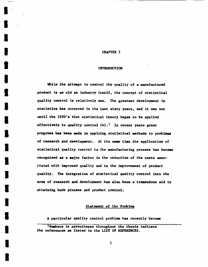
While the attempt t o control the qual i ty of a manufactured

product is as old as industry i t s e l f , the concept of statistical

qual i ty control is re la t ive ly new. The greatest development in

statistics has occurred in the last s ix ty years, and it w a s not

u n t i l the 1920's tha t s t a t i s t i c a l theory began t o be applied

e f fec t ive ly to qual i ty control (4) .1

progreats has been Bade in applying statistical methods to problems

of research and development.

s t a t i a t i c a l qual i ty control t o the manufacturing process has become

recognized as a major factor i n the reduction of the costs asso-

ciated with improved qual i ty and i n the improvement of product

quality.

area of research and development has a l so been a tremendous a i d in

a t ta in ing both process and product control.

In recent years great

A t the same time the application of

The integration of s t a t i s t i c a l qual i ty control i n t o the

Statement of the Problem

A par t icu lar qual i ty control problem has recently become

'Numbere is parentheses throughout the thes i s indicate the references as l i s t e d in the LIST OF REFEFUDICES.

1

2

cvident in the field of aerospace telemetry. Aerospace telemetry

l a the "science of transmission of information from air and space

vehicles to accessible locations" (15).

The advent of the missile age has brought about a pheno-

With the m e ~ l increaae in the usage of telemetry equipment.

evolution of new techniques and equipment for telemeterlng in-

flight apace vehicle data, the need for increased accuracy and

precision of the transmitting equipment is obvious.

teleaetry package2 ie placed on the spacecraft for the purpose

of transritting the most critical measurements to a telemetry

ground station. At the ground station personnel continuously

monitor and analyze these measurement data to determine the effect

of flight conditions at the vehicle.

necessity for the telewtry package to be of sufficient quality to

assure that the transmitted data is actually that measured at the

An airborne

Therefore it is of prime

vehicle.

During the t h e required for each telemetry package to be

sent from the manufacturer to the space vehicle, there are several

places where the control of the quality of the package needs to

be utabltehed. The first of these is at the manufacturing plant

hmedlately before hipping the package to the telemetry personnel.

Another is at the test laboratory immediately after the telemetry

LA telemetry package is an electrical system coneleting of a set of subcarrier oscillators for converting measured voltage into frequency, a dxer amplifier, a transmitter, and a paver amplifier used for transmitting signals from space vehicle to a ground receiving station.

8 1 -

8 I I I 1 I 1 8 0 8 I 8 B 8 1 1 8

3

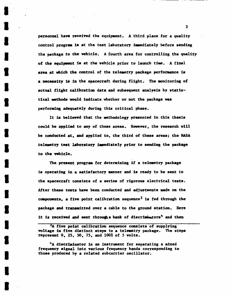
pernounel have received the equipment. A t h i rd place fo r a qua l i ty

control progrm is at the test laboratory lmed ia t e ly before sending

the package t o the vehicle. A fourth area f o r controll ing the qua l i ty

of the equipment Sa a t the vehicle pr ior t o launch tire, A f i n a l

area at which the control of the telemetry package performance is

a necessity is in the spacecraft during f l i gh t . The m i t o r i n g of

ac tua l f l i g h t ca l ibra t ion data and subsequent analysis by statis-

tical methods would indicate whether or not the package u a ~

performing adequately during th i s critical phase.

It la believed tha t the ethodology presented i n t h i s t hes i s

could be applied t o any of these areas, However, the research vi11

be conducted at, and applied to, t he th i rd of these areas; the M A

telemetry test laboratory imedia te ly p r io r t o sending the package

t o the vehicle.

The present program for dettnnfning i f a telemetry package

ie operating in a sa t i s fac tory manner and is ready t o be sent t o

the spacecraft consists of a series of rigorous electrical tests.

After these tests have been conducted and adjustments made on the

components, a f ive point cal ibrat ion sequence3 is fed through the

package aud t r h t t e d over a cable t o the ground s ta t ion .

it is received and sent througra bank of d i s c r ~ o r s 4 and then

Eere

f i v e point ca l ibra t ion sequence consists of supplying voltage in f i v e d i s t i n c t s teps t o a telemetry package. represent 0 , 25, 50, 7S, and 100% of 5 vol t s .

The s teps

4A discrlminator is sn instrwnent f o r separating a mixed frequency signal in to various frequency bands corresponding t o thoae produced by a re la ted subcarrier o sc i l l a to r .

4

recorded by an oscillograph.

is at present the only meam for d y z i n g the qual i ty of the

assembled package.

inconclusive answers t o the questions "what is the accuracy and

precisian of the package?"

of varirtiaap within the package?"

systematic e r ro r s while precision is a measure of rand- (chance)

errors (5,6) .

This record made by the oscillograph

It is thought tha t t h i s method furnishes

and "are there auy assignable causes

Accuracy is a measure of

The researcher believes t h a t by establ ishing an ef fec t ive

program of qual i ty control u t i l i z ing statistical apethods, these

questions can be answered and u l t ina te ly a decision t o reject o r

accept the package as sat isfactory can be made. Also, through

the establishment of a qua l i ty control pragrla a quant i ta t ive

h is tory of the perforumce of telemetry packages can be assembled.

The Proposed He thodolorn

The methodology employed i n the establishment of t h i s qual i ty

control program vi11 assure that t he basic components of the

telemetry package, the subcarrier o sc i l l a to r s , are i n statis-

tical control.

control of product qual i ty by Shewhart control charts.

control char ts w i l l provide a graphical method for comparing with

The methodology is based on the statistical

These

5An oscillograph is a device f o r producing a writ ten curve representing variable voltage.

5

an average value t h e output of the d i f fe ren t subcarrier o sc i l l a to r s

over several levels of input voltage.

(henceforth referred to as SCO's) which d i f f e r s ign i f icant ly from

the overall mean value may be investigated fo r assignable causes

of variation and subsequently replaced i f abnormalities exis t .

Therefore subcarrier o sc i l l a to r s

There are two d i s t inc t but re la ted phases of control chart

analysis (10).

w i t h No Standard Given," the control chart is used as a device

f o r specifying a state of statistical control and judging whether

the state of control has been attained based on past data.

purpose in t h i s phase is thus to discover whether measurements from

samples vary among themselves by an amount greater than should be

a t t r ibu ted t o chance.

With Respect t o a Given Standard," is used t o discover whether

nrerSuremnts obtained i n current production depart s ign i f icant ly

from "standard values" which may have been established by experience

based on pr ior data, by economic considerations, or by reference

t o the desired state of t h e process as designated by the

specifications.

applied t o the f i r s t of these phases.

will therefore be t o judge whether a state of control has been

at ta ined f o r the SCO's and then to specify a goal of statistical

control f o r future action.

In the f i r s t h e , which is often termed "Control

The

The second phase, usually ternred "Control

The methodology developed i n t h i s t hes i s w i l l be

The r e su l t of the analysis

Following a brief discussion of the general theory of qual i ty

control i n CEAPTER 11, a theoret ical development of the methodology

consists of two types of control charts.

standard deviafions ( u - chart ) is used f o r analyzing the

The control chart f o r

6

var i ab i l i t y of the SCO's.

(x - chart) supplies a basis f o r judging whether the various ?I

values, the meun values f o r each SCO-input level grouping, are in

8t8tlstical control.

properly w i t h respect t o e i t h e r t h e i r arean values or t h e i r varia-

The control chart f o r mean values

Therefore SCO's which are not functlonlng

b i l i t y can be quickly detected and investigated.

umignable -em have been removed, t he performance of the SCO's can

After these

be predicted and standards se t f o r t h e i r va r i ab i l i t y and rean values.

These standards can then be used f o r the evaluation of future

telemetry package performance.

A second major area of investigation is the development of

the operatlag characteristic (OC) function for the char t f o r

means and the chart f o r standard deviations f o r analpls barred on

put data. The OC functions a re developed In CBAPTER IV, and a

general procedure Is given for obtaining the OC curve fo r both

A t h i rd major problem t o be considered i n t h i s thes i s is

the determination of the proper l i m i t constant, K, t o be used in

calculating the c m t r o l chart llmits. The selection of the

proper K factor requires considerable analysis, and the decision

llut be baaed on an economic evaluation of the risks involved in

making incorrect decisions. This problem is solved i n QIAPTER V.

I f the thes i s is to have any prac t ica l significance, the

methodology must be applied to an actual s i tua t ion and meaningful

r e su l t s obtained. Therefore, a f i n a l major thes i s contribution is

1 8 1 - 1 I 8 I I I 8 8 I I I I I 8 I 1 I

7

an investigation of the aethodology applied to a real world

environment in CHAPTER V I ,

telcactry ground etatian at the Marshall Space Flight Center in

Huntsville, Alabama,

by obscrring the ability of the control charts to detect certaln

dfunctioning caaponento in a telemetry package set-up, Finally

what the control charts indicate that the experimental package is

in statistical control, the precision and accuracy of this package

i8 88tfaated.

An experiment was performed in the

The application of the methodology is tested

.

"A control chart i~ a s t a t i s t i c a l device pr incipal ly used

for the study and control of repet i t ive processes" (4).

discovery and development of control char ts w e r e made i n 1924 and

t h e f o l l w i n g years by a young physicist of the Bell Telephone

Uborator ies , Walter A. Shewhart.

which w a ~ complicated by the presence of random variat ion, he

decided that the problem was statistical i n nature.

observed varhtion i n performance vas inherent i n the process and

could be explained as being the r e s u l t of chance causes.

var ia t ion was unavoidable. However, from time t o time variation8

occurred which could not be explained by chance alone, but were

the r e su l t of some change in the process. The d i f fe ren t ia t ion of

these two c r r a ~ e ~ of quality variation is the bas i s f o r the theory

of control arts .

The

In t rying t o solve a problem

Some of the

This type

If 8 group of data is studied and it is found that t h e i r

v r r i a t i a n conforps to a s t a t i s t i c a l pat tern that might reasonably

have been produced by chance causes, then i t is assumed that there

has been no change in the procers; i.e., there a r e no assignable

causes of var ia t ion present, and the process is said t o be i n

8

8 8 - 1 1 U I 1 I 8 I 8 8 I 8 I 8 I I 8

9

%tatistical control.'' If, however, the var ia t ions i n the data do

not confow t o a pat tern tha t might be expected by chance causes,

then it is concluded tha t one o r more assignable causes are a t work,

and the process is said t o be *'out of control."

etatietical pat tern of variation is described as follows.

The nature of t h i s

Suppose samples of a given size are taken a t regular in te rva ls

and suppose that f o r each sample soee statistic X (sample mean,

a u p l e etandard deviation, etc.) is computed. Since t h i s s ta t is t ic X

ir a sample r e su l t it w i l l be subject t o sampling fluctuations.

I f there are no assignable causes of var ia t ion present, these

sampling f luctuat ions w i l l t a k e the form of some def in i t e statis-

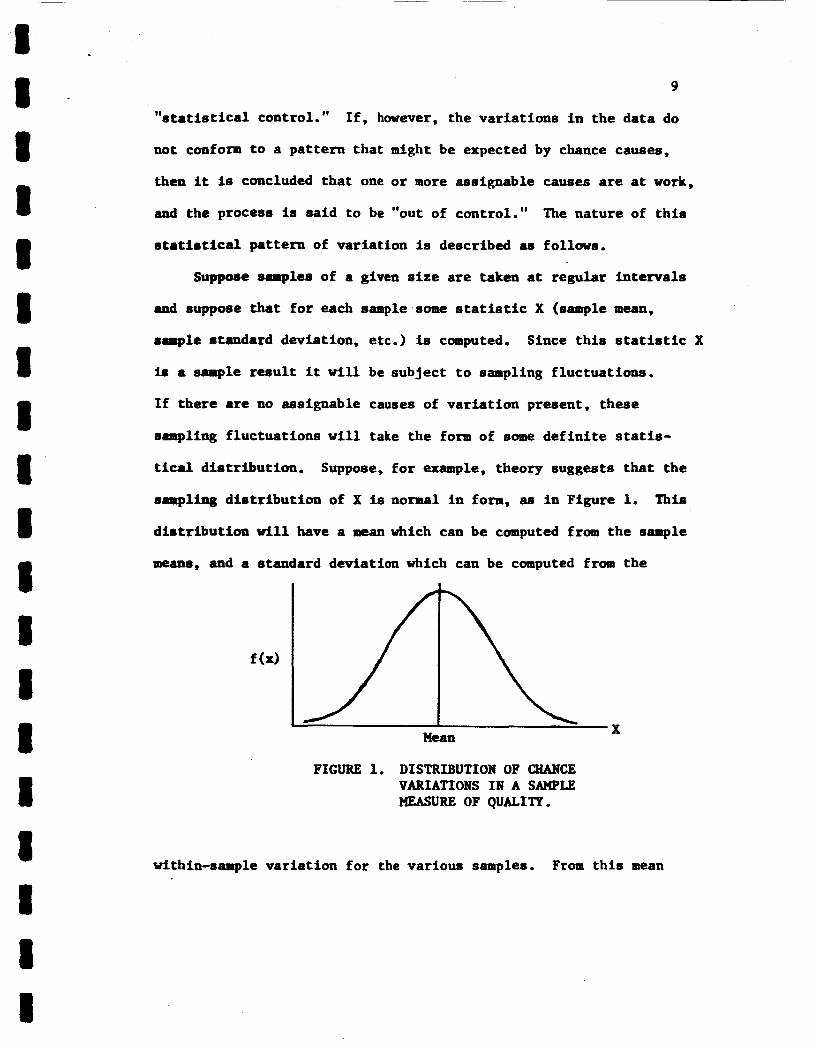
tical dis t r ibut ion. Suppose, f o r example, theory suggests t ha t the

sampling d is t r ibu t ion of X is normal i n form, as i n Figure 1. This

d i s t r ibu t ion vi11 have a mean which can be computed from the sample

means, and a standard deviation which can be computed from the

FIGURE 1. DISTRIBUTION OF QiANCE VARIATIONS IN A SAMPLE MEASURE OF QUALITP.

within-sample var ia t ion fo r the various samples. From t h i s mean

10

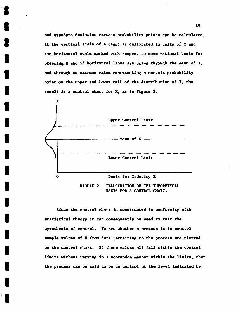
and standard deviation certain probabili ty points can be calculated.

I f the vertical scale of a chart is calibrated i n units of X and

the horizontal scale marked with respect t o some rational bas is f o r

orderfag X and i f horizontal l ines are drawn through the mean of X,

and through QL extreme value representing a cer ta in probabili ty

point on t he upper and lover ta i l of the d is t r ibu t ion of X, the

remult is a control char t f o r X, as i n Figure 2.

X

Upper Control L i m i t - - - - - - - - - - - - - - - - -

Mean of x

---- - - - - - - - - - ---- Lower Control L i m i t

0 B a s i s f o r Ordering X

FIGURE 2. ILLUSTRATION OF TEE THEORETICAL BASIS FOR A CONTROL CURT.

Since the control chart is constructed i n conformity with

mtatirrtical theory it can consequently be used t o test the

hypothesis of control.

sample values of X from data pertaining t o the process are plotted

on the control chart. I f these values a l l f a l l within the control

limits without varying i n a nonrandom manner within the l i m i t s , then

the process can be said t o be in control a t the l eve l Indicated by

To see whether a process is i n control

11

the chart.

from the pattern are investigated and assignable causes are tracked

down. After a condition of control has been sa t i s f ac to r i ly established,

departure from the condition may be quickly detected by maintaining

a control chart on current output (3).

I f the data do not conform t o t h i s pat tern then departures

8 I 8 1 8 I I I R 8 8 8 I)

8 1 8 1 1 1

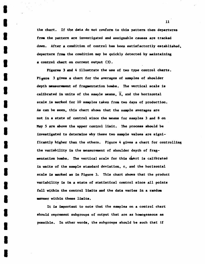
Figures 3 and 4 i l l u s t r a t e the use of two type control charts.

Pi- 3 gipas a chart fo r the averages of samples of shoulder

depth aeasurement of fragmentation b d s .

cal ibrated in uni t s of the sample means, X, and the horizontal

scale is marked f o r 10 samples taken from two days of production.

As can be seen, t h i s chart shows t h a t the sample averages are

not i n a state of control since the means f o r samples 3 and 8 on

May 5 are above the upper control l i m i t . The proceus should be

investigated t o determine why these two sample values are s igni-

f ican t ly higher than the others.

the va r i ab i l i t y i n the measurement of shoulder depth of frag-

mentation bambs.

i n units of the sample standard deviation, u, and the horizontal

scale is marked as i n Figure 3.

va r i ab i l i t y is i n a state of statistical control s ince a l l points

f a l l within the control linits and the data var ies i n a random

manner within these limits.

The vertical scale is -

Figure 4 gives a chart fo r controll ing

The ve r t i ca l scale fo r t h i s &rt is cal ibrated

This chart shows tha t the product

It is important t o note that t h e samples on a control char t

should represent subgroups of output tha t are as homogeneous as

possible. In other words, the subgroups should be such tha t i f

0 . 445

0.440

0.435

0.430

12

Upper Control L i m i t

Hean of x

Lower Control L i m i t

- - - - - - - - -

_ - - - - - - - - - -- 0 1 2 3 4 5 6 7 8 9 0 1 2 3 4 5 6 7 8 9 0

Map 5 %Y 6

FIGURE 3. CONTROL CHART FOR ?I FOR SHOULDER DEPTH OF FRAGHENTATION BaMBS (1).

0.010 4 Upper Control - - - - - - - - - - - - I- L i d t

0.005 - Mean of Q

Lower Control L i m i t

- - - - - -----a- 1 1 1 1 1 1 1 1 1 l 1 1 1 1 1 1 1 1 1 1

0 1 2 3 4 5 6 7 8 9 0 1 2 3 4 5 6 7 6 9 0 b Y 5 6

FIGURE 4. CONTROL CHART FOR e FOR SHOULDER DEPTH OF FRAGMENTATION BOMBS (1).

assignable causes are present, they w i l l show up i n differences

between the subgroups rather than i n differences between the

members of a subgroup (13) . would be the output of a par t icu lar subcarr ier o sc i l l a to r .

system consisted of say 10 subcarrier o sc i l l a to r s , it would be

b e t t e r to take a separate sample from the output of each SCO than

t o have each sample made up of items from a l l 10 S a ' s .

differences between the subcarrier oscillators may be an assignable

A natural subgroup, f o r -le,

I f a

For

‘I 1 - 8 I 8 I 8 B 8 8 1 8 1 1 I I I I 8

cause tha t is the object of

A control chart , then,

13

t h e control chart analysis t o detect.

provides a reasonable test fo r deter-

aining when a process can be considered t o be i n control.

advantages which may accrue when a process is brought i n t o good

control by control chart a n a l y s i s are ( 8 ) :

Solw of the

1,

2,

3.

4.

5.

ThC act of get t ing a process i n t o good statistical control ordinar i ly involves the ident i f ica t ion and removal of undemirable assignable causes. Hence, qual i ty performance haa been u c h improved.

A process i n good s t a t i s t i c a l control is predictable.

I f our process is in good statist ical control, w e can more safely guarantee our product.

A chart i n control i n experimentation enables us t o determine soundly the experimental error.

The sound way t o cut inspection is through get t ing the process i n control.

CHAPTER 111

THE DEVELOPMENT OF THE " H O ~ L O G Y

It has been s ta ted tha t the major problem t o be investigated

i n t h i s thes i s is the use of control char ts f o r determining whether

a telemetry package is i n a state of s ta t is t ical control.

two previous chapters the problem w a s discussed i n general. The

purpose i n t h i s chapter is t o develop a theore t ica l foundation

f o r the control chart models.

In the

Let us consider t he telemetry system as a type of indus t r ia l

process. The basic component of the telemetry package, the SCO,

may also be thought of as a sub-process. An analegous s i tua t ion

would be a la rge factory within which there are several manu-

facturing divisions. W e might be interested i n comparing these

manufacturing divis ions to determine whether they are producing

essent ia l ly the same output.

not seem applicable i f we were only interested i n comparing the

output of one entire factory with perhaps three other such factor ies .

However, the individual divisions within each factory would produce

a r epe t i t i ve output which could be analyzed by control chart techniques.

Therefore, w e s h a l l view each SCO as a manufacturing divis ion and as

Control char t analysis would cer ta inly

14

1 15

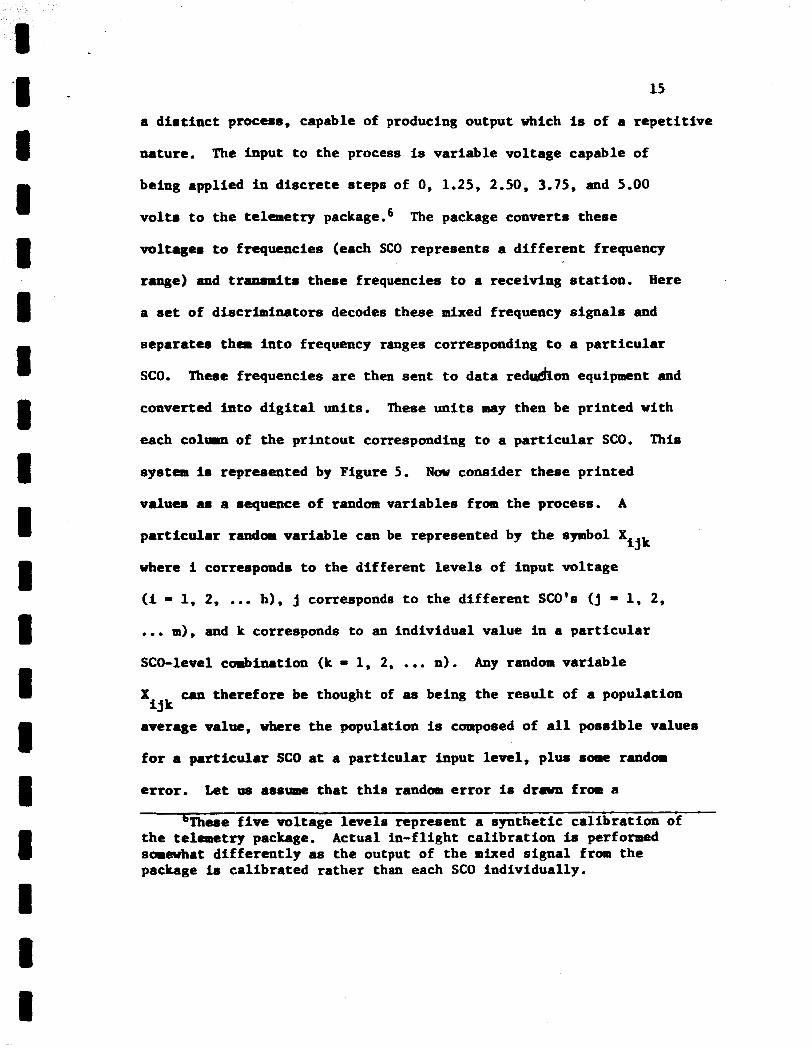
a d i s t i n c t process, capable of producing output which is of a repe t i t ive

nature. The input to the process is variable voltage capable of

being applied in discre te s teps of 0 , 1.25, 2.50, 3.75, and 5.00

vo l t s to the telemetry package.6

voltages to frequencies (each SCO represents a d i f f e ren t frequency

The package converts these

range) and trursrita these frequencies to a receiving s ta t ion .

a set of discriminators decodes these mixed frequency s igna ls and

separates t h a into frequency ranges corresponding t o a par t icu lar

SCO.

converted into d i g i t a l units.

each colrrn of the printout corresponding t o a par t icu lar SCO.

system i~ represented by Figure 5. Now consider these printed

value8 as a sequence of random variables from the process. A

par t icu lar random variable can be represented by the symbol X

where 1 corresponds to the different leve ls of input voltage

(i = 1, 2, ... h) , j corresponds t o the d i f fe ren t S a ' s (j = 1, 2,

... m), and k corresponds to an individual value in a par t icu lar

SCO-level combination (k - 1, 2, ... n). Any random variable

X

average value, where the population is composed of a l l possible values

f o r a par t icu lar SCO at a par t icular input level, plus some random

error. L e t us ass- tha t t h i s randam error is drawn from a

Here

These frequencies are then sent t o data re&m equipment and

These u n i t s may then be printed with

This

i j k

can therefore be thought of as being the r e su l t of a population ij k

bThccle f i v e voltage leve ls represent a synthet ic ca l ibra t ion of the telemetry package. somewhat di f fe ren t ly as the output of the mixed s ignal from the package 1s cal ibrated rather than each SCO individually.

Actua l in-fl ight ca l ibra t ion is perfomed

1 8 - I I I I I I I 1 I I I I I 1 I I I

c

s o x 1

PACKAGE SCO#2 VOLTAGE

SOURCE * e

e

16

+ TRANSMITTER

b

#I

#Z SEL

. REDUCTION EQUIPMENT

4

RECEIVER c DISCRIMINATORS . )I DATA

.

1

PRINTER

FIGURE 5. BLOCK D U G W OF THE FM/Fn EXPERIMENTAL TELEMETRY SYSTEM.

1 I - 1 1 u 1 I 1 I I I 1 1 I I I I I 1

17

universe of errors tha t are s t a t i s t i c a l l y independent (the value

of any one e r r o r does not depend on the value of any other e r rors )

and are dis t r ibuted i n a normal d is t r ibu t ion with a mean value of

zero and with some amount of variation. W e s h a l l fur ther assume

t ha t the several possible population average values tha t we are

considering are drawn from son l a rge universe of average values

tha t are norral ly dis t r ibuted.

mean f o r a l l possible SCO’s at a par t icu lar level of input, and

there may be some amount of var iab i l i ty of the population averages

The mean value of t h i s universe is the

about t h i s mean.

values are s t a t i s t i c a l l y independent of the rand- errors and

Let us also assume tha t the population average

that the univerrre mean value and var ia t ion are fixed quant i t ies ,

but are unbimm to us and m u s t be estimated from avai lable data.

We MY pav express th random variable X by a l i nea r mathematical

model and list several statements c la r i fy ing the term in the model. i9k

‘ijk ?i;j + ‘ijk* i = l , 2 , ... h; j = l , 2, ...m; k = 1 . 2, .. , n ,

where,

1, the q j k are s t a t i s t i c a l l y independent and dis t r ibuted

according to N( 0, ui2 );7

2. tho? are s t a t i s t i c a l l y independent and dis t r ibuted

according to N( Zi, the ic are S ta t i s t i ca l ly independent of the “ i jk ;

uf2 1, where u$ = 02ui2;

3.

4. the and u i 2 are fixed but unknown. 13

’This notation indicates that the e r ro r s a re d is t r ibu ted according to a normal probabili ty dis t r ibut ion (see p. 21) with mean of zero and variance oi2.

18

W i t h t h i s model i n mind we s h a l l now turn t o the problem of

developing a set of decision rules fo r determining whether a

group of SCO's are i n s t a t i s t i c a l control with respect t o the

average values of the random variables associated with the d i f fe ren t

SCO'a. The t es t ing of the hypothesis of s t a t i s t i c a l control in t h i s

-r ir termed "cmtrol through the use of the &hart,"

W e shall f i r s t formulate t h e hypothesis of control of the mean

value^ and the alternative hypothesis and then develop the %Chart

test f o r these hypotheses,

I f the SCO's arc i n a s t a t e of statistical control one

comaequence IE tha t the population average values f o r the various

SCO's are equivalent.

to the telemetry package, t h i s same voltage v f l l be applied t o

a l l the SCO'. 8imtltaneouely. Therefore, i f we d ig i t i ze the output

of these SCO's f o r a very long period of t i m e , and i f the SCO's

are known to be properly adjusted and functioning correctly, the

average of a l l possibh! digit ized values f o r any one SCO w i l l be

exactly the same a8 f o r a l l the other SCO's.

... - s. the n u l l hypothesis, symbolized by €Io,

sow reum any of the SCO'e have not been properly adjusted o r are

not functioning correctly, then a l l of the 2 equal. Thw iil # T2 # , , . # Xh, This is cal led the a l te rna t ive

In other words, i f we apply a cer ta in voltage

- - Thus Xi1 = Xi2 -

- This is the hypotheisis of control and is often termed

On the other hand, if f o r

values w i l l not be i j -

1 - 19

hfpothesis and is

hypotheses from a

l i s t e d on page 17

symbolized by H1.

s l i g h t l y d i f fe ren t viewpoint. Statement 2.

states t h a t the ?k

Let us examine these

are normally d is t r ibu ted with is wan

these zil will be equal and there w i l l be, of course, no var ia t ion

among thea. Therefore 8 wil l be zero. Hovever, i f any of the SCO's

are not functianing correctly, then these qj w i l l be unequal and

there w i l l be same variat ion aamng them.

than zero.

and variance e2ue2. Naw if a state of control exists, 1 1

Thus 8 w i l l be greater

Our two hypotheses may naw be s ta ted as:

H 8 - 0 ;

H ~ : e > 0 .

0 :

By t rea t ing the 2 88 random variables we are taking i n t o account

the average e f f e c t of m independent assignable causes of varying

magnitude.

par t icu lar s h i f t in the process averages, X'

size of the ?

is

Although we are unable t o specify t h e s i ze of any -

a measure of the 13'

as a group is given by the parameter 8. 13

Thus a test fo r the hypothesis of control, : 8 = 0 , would HO be t o compute each population average 3

with t he universe =an 2 If each 'sTe is exactly equal t o ? then

8 = 0 and the process I s in control.

impossible s ince each 2 values fo r a par t icu lar SCO, and the universe mean

value fo r a l l possible digi t ized values fo r a l l of the SCO's at a

given voltage level . W e would have t o l e t the process run for an

i n f i n i t e period of t i m e t o assemble these values.

and campare these values $3

1. 13 i' flQyever, t h i s method is

is an average of a l l possible d ig i t ized 19

is an average

Therefore, we must

8

20

f ind some awthod fo r tes t ing H

estimates of these population and universe parameters.

tha t w i l l be based on sample 0

Let us take a sample of n values of X for a par t icu lar i j k

SCO. The me!an value of t h i s sample is given by

We maat show t ha t the expected value of t h i s sample mean for an

i n f i n i t e d e r of samples of s i z e n is In other words, w e if must shaw tha t

This can be done by using elementary theorems of expectation

(see &prendix A, p. 8 6 ) as follows:

n = I - E E(X

i j k ) n k-1

It can also be shown In t h e same manner tha t the expected value of - x' is E- Thus,

i J i-

21

walwe are saqle ra ther than population means Nov eince tbese

there w i l l be some amount of variation among them tha t can be

a t t r ibu ted t o chance caueee. A measure of t h i s amount of var ia t ion is

i j

given by what is termed the standard e r ror of the mean, symbolized

. The standard error of t h e me- is merely a standard by %j deviation computed from the warious 'ii

defined by the formula

about zi. This term is i f

.

The r values w i l l therefore form some statistical dis t r ibut ion, i j

This d is t r ibu t ion 2 of which the mean i s and t h e variance is uzij.

of .L~M values w i l l approach a normal (Gaussian) d i s t r ibu t ion

regardless of the dis t r ibut ion of individual X values. The

frequency function of t h i s dis t r ibut ion is given by i j k

This f ac t is a t t r ibu ted to the cent ra l l i m i t theorem of statistics

which states, "The form of the d is t r ibu t ion of sample means

approachas the fora of a noraal probabili ty d is t r ibu t ion as the

size of the sample is increased" ( 9 ) .

Thus, the probability for any 51 t o l i e between any two i J

standard wrlues Ti + Ku- and c- can be found by inte- xij

8 - E 1 1 t I I 8 1 I 1 E 8 8 8 I

, a ' 8 I

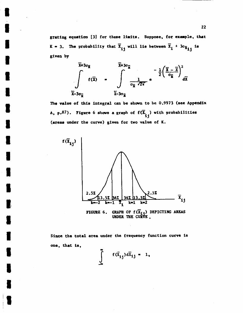
22

Suppose, for example, that grating eqtmtion (3) for these limits.

K = 3, The probability that will l i e betveen Zi * 30- is

given by 13 =I3

- +(y)2 - e dx

- - - - x-3uz X-3Uz

The value of this integral can be shown to be 0.9973 (see Appcadix

A, pJ37).

( a r m under the curve) given for two value of K.

Figure 6 shows a graph of f(x ) with probabilities i J

FIGURE 6. GRAPH OF f (q ) DEPICTING A R E S UNDER 3SiE CUB&.

Since the total a r a under the frequency function curve is

one, that is, m

J -a

8 I I I

23

t h e area outside limits of E * 30- Therefore, the probabili ty that x

i j

limits due t o chance alone i e 0,0027.

eas i ly be computed for other values of K.

is 1 - 0,9973 - 0.0027. i xiJ

w i l l f a l l outside t h e s e

This probabili ty could

I f was previously indicated tha t the expected value of

ir zc. However , the expected value of a- is not a: Sample

variances used t o estimate population variances tend to be

consistently small by a factor of (n-l)/n (see ~ 2 7 ) .

t o correct f o r t h i s "bias," u-

i j

xi9 x i j

Therefore,

must be multiplied by xiJ

t o give an unbiased estimate of . In computational fora t h i s

unbiased estimate is given by

Thus, t o test the hypothesis of statistical control, %: 8 - 0 ,

we w i l l set the * K8- l i m i t s f o r a par t icu lar value of K and xij -

then observe whether the computed xij values f a l l within these

limits. I f a l l ?I are within the l i m i t s , we w i l l assume that

the SCO's are i n statistical control. However, i f any f a l l s

outside the limits, we w i l l assume that an assignable cause of

ij

13

var ia t ion has occurred and t h i s par t icu lar SCO must be investigated.

We must rea l ize tha t there is a cer ta in risk involved i n

making an incorrect decision. A point might f a l l outside the limits

8 due merely to chance.

SCO fo r no reason. This type of decision e r ro r is cal led a Type I

error and the associated risk: i.e., the probabili ty of coarmitting

t h i s error, is termed the a risk.

t ha t an SCO which has an assignable cause of var ia t ion would be i n

control due to its 5

decision error is called a Type I1 e r ro r and the associated r i s k

is termed the 8 r isk.

subsequent chapters.

they exist.

In t h i s case w e vou-- -e invest igat ing an

On the other hand, w e might conclude

f a l l i n g within the l i m i t s . Th i s type of i j

A n ana lys i s of these risks vi11 be given i n

It w i l l suf f ice at t h i s point t o r ea l i ze tha t

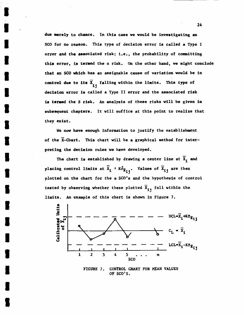
W e now have enough information t o j u s t i f y the establishment

of t he y-Chart.

pret ing the decision rules we have developed.

This chart w i l l be a graphical method for inter-

The chart is established by drawing a center l i n e at zi and

Values of 51 are then i j

placing control l imi t s a t Ti * ~ 6 -

plot ted on the chart for the m SCO's and the hypothesis of control

tes ted by observing whether these plotted ?I

l imits .

X i j

f a l l within the i j

An example of t h i s chart is shown i n F igure 7.

4 E l

1 2 3 4 5 . . . m sco

FIGURE 7. CONTROL CHART FOR MEAN VALUES OF SCO'S.

I 8

25

We s h a l l now turn t o the problem of developing a control chart

fo r t e s t ing the va r i ab i l i t y within the d i f fe ren t SCO's.

The o-Chart

In t h i s sect ion the problem t h a t w e are involved with is t o

develop a set of decision rules f o r determining whether a group of

SCO's are i n statistical control with respect t o a measure of

va r i ab i l i t y of the random variables associated with the d i f fe ren t

S O ' S .

deviation, u*

One such measure of the v a r i a b i l i t y is the standard

i j

W e s h a l l once again formulate the hypothesis of control of the

standard deviations and the a l te rna t ive hypothesis and then develop

the o-Chart t o test these hypotheses.

F i r s t , let us make t h e assumption tha t the various X values i j k

are normally distributed.

assumption. However, theoret ical ly w e know nothing about the

frequency function of the standard deviation of samples from a

non-normal universe. Therefore, i n order t o develop the method-

ology ve w i l l assume normality and then later analyze the e f f e c t s

of non-normality.

This is perhaps a ra ther r e s t r i c t i v e

This hypothesis of control f o r va r i ab i l i t y is tha t the pop-

ulat ion standard deviations f o r the SCO's are equal.

ui1 = ai2 - ... = o& . frcun a universe of standard deviations whose average value is a;

Thus,

Now suppose tha t these o i j values come

26

and whose variance is ai2- O2ui2.

then e w i l l be zero.

population standard deviations w i l l be unequal and 8 w i l l be greater

than zero.

I f a state of control exists

If the process is not i n control, then the

Once again the two hypotheses may be s ta ted as:

%: e - 0 ;

H ~ : e > 0 .

Aa with the t e s t i n g of the hypothesis fo r the man values, w e

know t ha t it is impossible to ca lcu la te a true population standard

deviation s ince t h i s would indicate a deviation of a l l possible

X

on sample estimates f o r our test.

values about t h e i r mean. Therefore, w e must once again r e ly i3k

Suppose tha t i n addition t o calculating sample averages,

Qj, we calculate sample standard deviations from the formula -

I n

The

u i j , fo r

is given

frequency function of the d is t r ibu t ion of variances,

samples of s i z e n from a normal universe and i ts d i f f e ren t i a l

by, momentarily dropping the i j subscript , (1)

where l'((n-1)/2) is the gannna or f a c t o r i a l function (see Appendix A,

p. 88 . Now changing the variable t o ai) i n equation 161 gives

8

a I I 8 8 I I I 1 8 1 8 1 8 R I

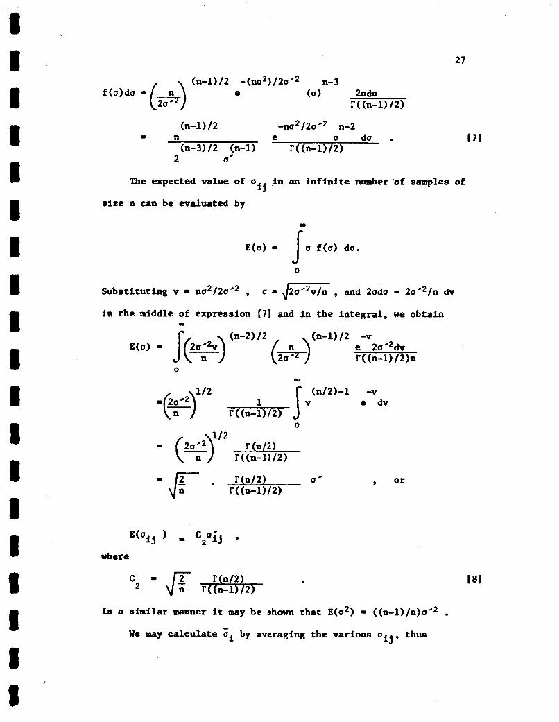
m - 27

e

2 U’

The expected value of a In an i n f l n i t e number of samples of 21

size n can be evaluated by

E(a) = (a f (a) da.

0

Substi tuting v - na2/2ac2 , u - ,/- , and 2ada = 2aa2/n dv

In the middle of expression [ 7 ] and i n the Integral , we obtain 0

(n-2) /2 (n-1)/2 -v e 2 ~ ~ 7 - d ~

0 .D

(n/2)-1 -v e dv

1/2 1

r((n-1)/2) 0

I \1/2

where

In a similar manner It may be shown tha t E(a2) = ((n-l)/n)aa2

W e map calculate ai by averaging the various a thus 51 ’

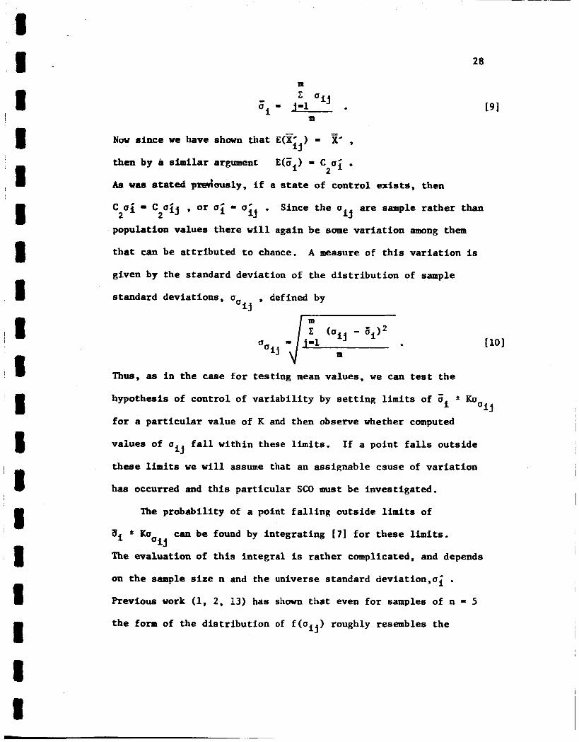
m a i j a' = j-1 .

m i

28

(91

- - Now since w e have shown tha t E ( F ) =

then by a similar argument

As was etated p d o u s l y , i f a state of control exists, then

X' , E(Gi) = C ui

i j

2

e Since the a are sample ra ther than c ui = c U i j , or ui = uij

population values there w i l l again be some var ia t ion among them i j 2 2

t h a t can be a t t r ibu ted t o chance. A measure of t h i s var ia t ion is

given by the standard deviation of the d is t r ibu t ion of sample

, defined by O U i j

standard deviations,

I m

Thus, a8 i n the case f o r tes t ing mean values, w e can test t h e

hypothesis of control of va r i ab i l i t y by se t t i ng l i m i t s of gi f Ku

f o r a par t icu lar value of K and then observe whether computed O i j

values of u f a l l within these limits. I f a point f a l l s outside

these limits w e w i l l assume t h a t an assignable cause of var ia t ion 53

has occurred and t h i s par t icular SCO must be investigated.

The probabili ty of a point f a l l i n g outside l i m i t s of

Tii * KO The evaluation of t h i s integral is ra ther complicated, and depends

can be found by integrat ing (71 fo r these l imi t s . u i j

on t h e sample size n and the universe standard deviation,ai . Previous work (1, 2, 13) has shown tha t even f o r samples of n - 5

t he form of the d is t r ibu t ion of f ( a ) roughly resembles the i j

I . 1 - I 8 I I 8 I 8 I 1 8 I 8 8 8 I I 8

29

normal dis t r ibut ion. As n Increases t h i s resemblance becomes

greater.

f a l l i ng outside the control l imi t s is not exactly the same ae fo r a

saaple ?I

equal.

for both charts.

19 Therefore, although the probabili ty of a sample u

let us asswe that these probabi l i t ies are roughly i J ' Thuu, the same! K factor can be used f o r determining the l imi t s

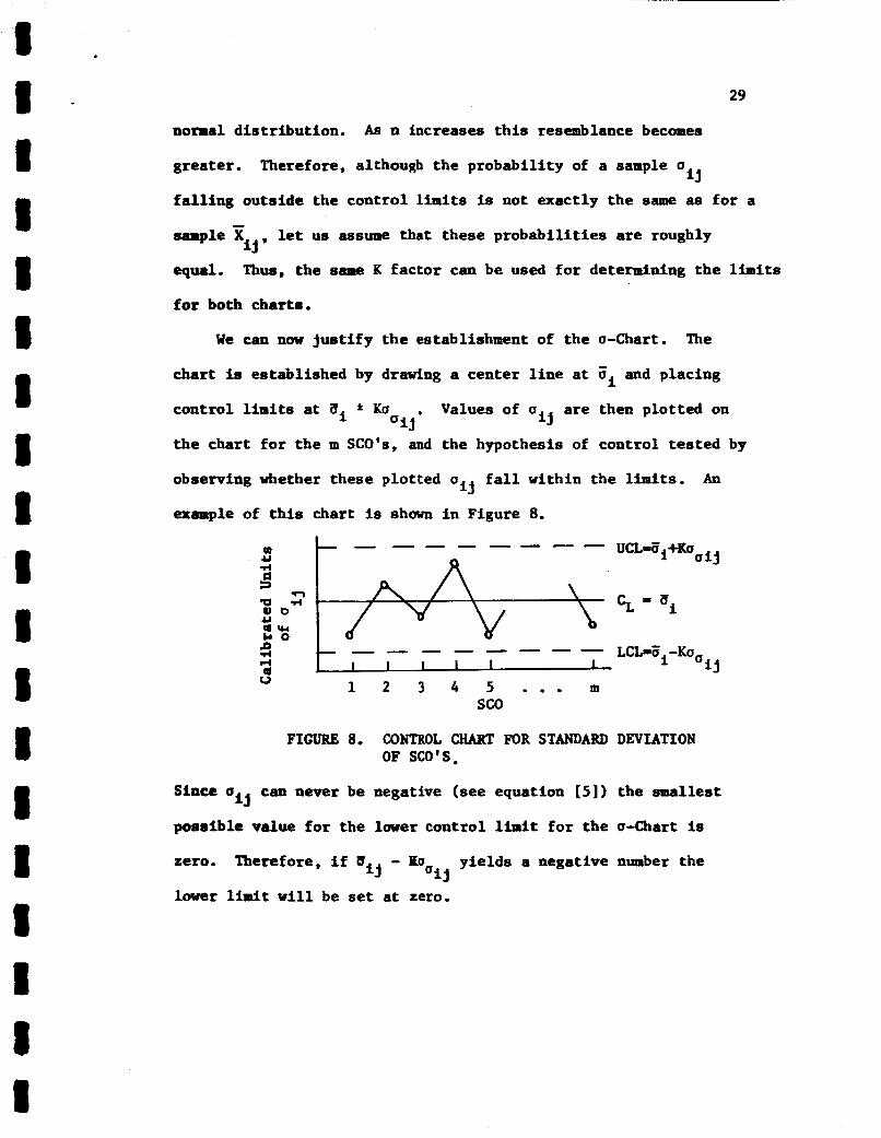
We can now j u s t i f y the establishment of the a-Chart. The

chart is established by drawing a center l i n e a t si and placing

control limits at tTi * KO . Values of u are then plotted on

the chart f o r the m SCO's, and the hypothesis of control tes ted by i j i J

observing whether these plotted u f a l l within the l imits . An

example of t h i s chart is shown in Figure 8.

- - - - - - - - LCLGi-KUu I I I I I i j 1 2 3 4 5 . . . m

SCO

FIGURE 8. CONTROL CHART FOR STANDARD DEVIATION OF SCO'S,

Since u can never be negative (see equation [ 5 ] ) the smallest

possible value f o r the lower control l i m i t f o r the u-Chart is i;l

zero. Therefore, if U - Eu yields a negative number the

lower lidt w i l l be set a t zero. i j Qij

8 8 - 8 1 1 I 1 1 8 U 1 8 I I 1 I I 8 1

30

Estimation of u0

Although the methodology f o r the %Chart w a s developed

I before the u-Chart, i n actual application of the control char ts

the a-Chart should be established f i r s t . The reason f o r t h i s is

tha t when the process va r i ab i l i t y is i n statistical control the

process standard deviation, d, may be estimated from the collected

data.

there is l i t t l e basis fo r estimating u4, and therefore l i t t l e basis

I f the va r i ab i l i t y of the process is not i n approximate control

fo r an X-mart. Recall from the previous sect ion tha t E(ai) - C uc .

2 i

Therefore, i f the SCO's are in control the universe standard

deviation f o r each l eve l of input voltage may be estimated as

2

where C is defined i n equation [8]. 2

Thus, estimate of the va r i ab i l i t y of the process may be

obtained by averaging the d i f fe ren t Oi values f o r the f ive

leve ls of input voltage, and

h c 81

e 0 = i=i h

It should be noted t h a t t h e r e are other methods available

f o r estimating u*. For instance, an estimate of the standard

deviation fo r each l eve l is given by

31

I m n

V mn

Once t h i s estimate is obtained equation [12) could be applied

t o give an estimate of u'.

The major advantages in the f i r s t method given over t h i s

method are:

1. The estimate of u* by the f i r s t method is on the average less than the corresponding estimate by the above method. Therefore, c r i t e r i a involving the use of the f i r s t method w i l l i n t h e long NU detect trouble more often than similar criteria involving t h e second method (13).

2. The estimate of u' by the f i r s t method involves the use of the 5 values which have already been calculated. The second methd requires considerable additional calculation. Therefore, a savings i n computational labor is brought about by the f i r s t method.

A th i rd method f o r estimating u' would be t o calculate

from the formula

U 4 4 -

112' [2(n-1) - 2n@]

a i - 2

where u

then apply 1121 to give 8'.

is defined by (10 J and C is def ined i n [SI, and uis 2

This method of calculating 6' can

be Shawn t o be val id by computing

E<u2) = J u2f (a)do, 0

where f 4o)da is given i n [7 ] , and then computing

[E(u2) - E(u)]~ , uU

uo - q .

8 I - 8 8 8 I 8 I I I 8 I I 8 1 I I I 1

32

This method gives essent ia l ly the same r e su l t as does the f i r s t

method. However, once again a savings i n computational labor

can be achiwed by using the first method.

There are other methods of estimating u d from the data.

However, the methods presented here are considered t o be the

most appropriate and therefore are the only ones mentioned.

Consequently, we s h a l l use the f i r s t method presented: i.e.,

the application of (111 and [12], t o estimate uc.

Effects of Non-Normality

It w a s assumed fo r the development of the u-Chart tha t the

d is t r ibu t ion of individual X values follows the normal d i s t r i -

bution. i j k

This assumption may not always be valid; therefore, w e s h a l l

discuss br ie f ly same of the e f fec ts of a non-normal population.

The primary l imi ta t ion caused by a non-normal population

is on the statement tha t t he probabili ty tha t a sample u

w i l l f a l l outside the a-Chart l imi t s is roughly the same as f o r

an 51

i s not normal t h i s statentent is not necessarily t rue since

ij

value f a l l i n g outside the ?I-Chart l i m i t s . I f the population i j

w e know nothing about t he frequency function of a sample standard

deviations from a non-normal universe.

Prwioua work with dis t r ibut ions of telemetry data have

indicated tha t although qui te of ten these d is t r ibu t ions are not

normal, they are usually unimodal' (7). The Camp-Meidel theorem

"A mimodal d i s t r ibu t ion is one which is monotonically decreasing on both s i d e s of its one modal value, o r value which occurs the most frequently.

I -

I

I I '

33

states tha t i f the dis t r ibut ion of t h e random variable X is unimodal,

the probabili ty tha t X should deviate front its mean by more than

K tlmes its standard deviation is equal t o or less than 1/2.25Kz

i j (4). It can be shown (13) that, although the dis t r ibut ions of a

of samples of n are not knovn fo r other than the normal miverse ,

nevertheless the moments of t h e d i s t r ibu t ions of u are known

i n teras of the moments of the universe. Hence, we can alvays i j

ecltablish limits

Ui * Ka aij

within which the observed standard deviation should f a l l more than

l O O ( 1 - 1/2.25K2) per cent of t he t o t a l number of times a sample

of n is chosen, so long as the qual i ty of product is controlled.

Now i f K - 3, lOO(1 - 1/2.25K2) = 95.1 per cent. This is compared

with a value of approximately 99 per cent i f the normality assump-

t ion holds. It is fur ther believed tha t the main cause of non-normality

i n telemetry data is peakedness ra ther than asymmetry.

possibly indicate tha t even a l a rger percentage of the sample

This would

values would f a l l within the limits than could be predicted by

the Camp-Meidel theorem. We s h a l l therefore f e e l j u s t i f i ed i n

select ing the stme K fac tor for both charts regardless of t he fora

of the d is t r ibu t ion of individual values.

The l imi ta t ion imposed by non-normality would become even

more evident i n t h e discussion of the operating charac te r i s t ic

function i n QiibPl'EIl IV. This function could not be evaluated with-

out the assumption of normality. Therefore, we w i l l recognize

I 1 . I B 8 I I 1 1 I 8 1 I I I 8 I 8 1

34

t he fact tha t the data may not be perfect ly normally d is t r ibu ted ,

but w i l l make the asslrmption of normality real iz ing tha t perhaps

we have introduced some er ror i n t o our analysis.

t h i s error w i l l not seriously a f f e c t the methodology and thus may

be tolerated.

It is believed tha t

Summary of the Methodology

The control chart methodology presented In t h i s chapter may

be suaaarized i n the following step-by-step procedure:

1. Obtain means and standard deviations f o r samples of s i z e n

for each of the j SCO's, and f o r each input leve l , from the formulas

n

i j k - C X X - k-1

n 53

/ n

J k:l:k - siz,, . 2. Compute an average mean, average standard deviation, and

standard error of the mean for each l eve l of input from the formulas

1 8 8 I I I B II 8 I I I 8 8 I 1 i I I

35

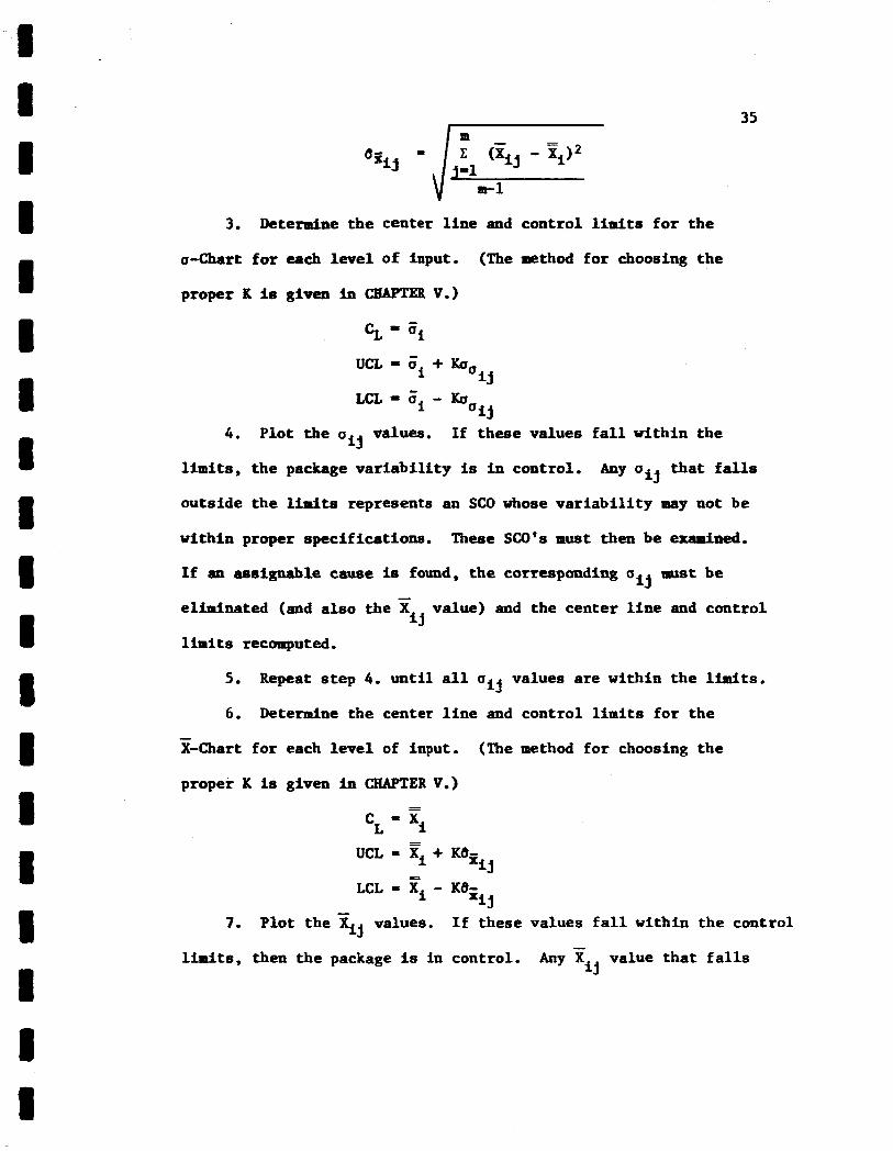
3. Determine the center l i n e and control limits f o r the

o-Chart f o r each level of input. (The method f o r choosing the

proper K is given in CEAPTER V.)

- L c L = u i - u

i j 4. Plot the o values. If these values f a l l within the

i j

l imi t s , the package va r i ab i l i t y is in control. Any oij that f a l l s

outside the limits represents an SCO whose va r i ab i l i t y may not be

within proper specifications. These SCO’s must then be examined.

I f an assignable cause is found, t he corresponding u must be $3 eliminated (and a lso the x limits recanputed.

value) and the center l i n e and control i j

5. Repeat s tep 4. un t i l a l l oij values a re within the limits.

6 . Determine the center l i n e and control l i m i t s f o r the - X-Chart fo r each level of input. (The method fo r choosing the

proper K is given in CHAPTER v.1

UCL = zi + KO- xij

7. Plot the values. I f these values f a l l within the control 3 limits, then the package is in control. Any zij value tha t f a l l s

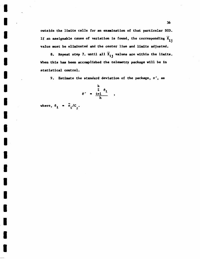
36

outside the limits c a l l s for an examination of tha t par t icu lar SCO,

If an assignable cause of variation is found, the corresponding E value must be eliminated and the center l i n e and limits adjusted,

i j

8. Repeat s tep 7. u n t i l a l l values are within the limlts. i j

When t h i s has been accomplished the t e l e w t r y package w i l l be i n

statistical control.

9. Estimate the standard deviation of the package, u), as

h

- where, bi - u /C .

$ 2

CHAPTER I V

THE DEVELOPHENT OF TEE PROBABILITY

FUNCTIONS F’OR THE TPPE I AND TYPE I1 ERRORS

In the f i r s t par t of CHAPTER 111, w e s ta ted i n terms of a

mathematical d e l , tha t there are two poss ib i l i t i e s f o r the

state of control of the telemetry process.

(a) Process i n Control

H e r e we assume that t he d is t r ibu t ion of the process (i.e.,

the dis t r ibu t ion of individual items of product) is normal

vith a fixed mean Ti, and fixed standard deviation a;,

both rmltnown.

(b) Process out of Control

In t h i s case we again assume tha t the d is t r ibu t ion of

the process (at any par t icu lar time) is normal with fixed

but &own standard deviation ui, but now the process

mean la regarded a~ a chance quantity i t s e l f , having a

-mal dist r ibut ion with unknown mean and standard

deviation 0ui where 8 is a posi t ive constant,

S t a t e (b) w a s later given i n terms of the standard deviation as a

chance quantity having mean value a i and standard deviation ea;,

37

38

n cp - 0 P ) I U a m U m

n n U

P) U 4 U v)

7 rn I W

1 I - I 1 I I 1 1 I I I 1 I I II I I I I

39

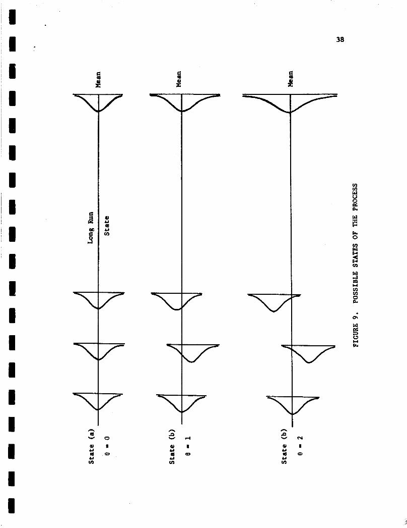
It was also shown tha t state (a) is a special case of state (b)

when 8 - 0 , Both of these s t a t e s are i l l u s t r a t e d i n Figure 9,

where several poss ib i l i t i e s are shown corresponding t o various

values of 8 (10,ll).

Since e i t h e r of these s t a t e s may be present, ve are con-

fronted with two types of errors , am vaa s t a t ed previously.

we may get out-of-control points on t he char t when the process

is actual ly i n control.

Type I error .

points when the process level is actual ly shif t ing.

t h i s happening is the Type I1 error .

F i r s t ,

The chance of t h i s occurring is the

On t he other hand, w e may get no out-of-control

The chance of

In t h i s chapter we w i l l develop a probabili ty function f o r

both char t s tha t w i l l enable us to study these errors f o r various

sample sizes, n, and for various control l imi t factors , K.

The probabili ty function for the s i z e of the Type I1 er ror ,

6, is cal led the operating characteristic (OC) function and asso-

ciated with t h i s function is t h e OC curve, The OC cumre fo r a

control char t used t o study past output shaws the probabili ty of

a l l m sample points f a l l i n g inside the control limits.

given set of sample data studied, t h i s probabili ty is expressed as

a function of the actual process charac te r i s t ics . Therefore, t h i s

curve gives a graphic picture of t he a b i l i t y of the control chart

to detect trouble.

For the

L e t us then f i r s t turn t o the development of the operating

charac te r i s t ic function f o r the h h a r t .

40

Operating Characteristic Function fo r the %Chart

The operating character is t ic function f o r the %Chart gives

the probabili ty tha t , for a selected value of the l i m i t constant

K, a l l of the m sample

as a function of a given value of the process mean.

values will f a l l within the control l i m i t s

This value can

be represented by the process mean under control conditions plus

some quantity 6, which indicates a s h i f t i n t h i s mean. In

symbolic notation t h i s probability function may be s ta ted as

.. . - -

where Fg - I(* + 6.

Thus w e wish t o evaluate (151 f o r various values of K, n, and 6.

F i r s t let us attempt t o simplify [ls]. By transposing the

X and dividing by 82 i n each inequality w e obtain

- - The quantity Zj - (zj - X ) i U i is dis t r ibuted as a modified "t"

dis t r ibu t ion hum as the Hotelling T2 dis t r ibu t ion (4). This

d is t r ibu t ion is often ra ther d i f f i c u l t t o work with i n solving

theoret ical problems. Therefore, w e s h a l l assume t h a t 2 is

approxlmately dis t r ibuted as a normal d is t r ibu t ion w i t h a mean of j

zero and a variance of one (see Appendix A, p. 87 1. W e must rea l ize

tha t some error is Introduced by t h i s assumption. However, the

error introduced due t o the complexity of the solution of OC function

when the Hotelling T2 dist r ibut ion is used i n thought t o be more

than the e r ro r due t o the normality asswaption. Also, hypotheses

41

t e s t ing when n o m l i t y is assumed is more conservative than when a

"t" dis t r ibu t ion is assumed. Thus, w e wish to evaluate, for

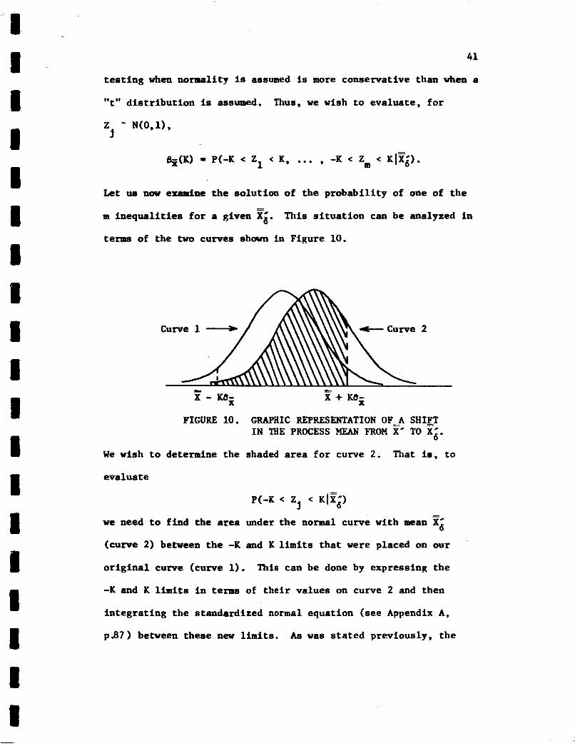
Let UB PQV examine the solution of the probabili ty of one of t he

m inequal i t ies for a given zi. terms of the two curves shown i n Figure 10.

This s i t ua t ion can be analyzed i n

Curve 1 + -Curve 2

/&\\\\\\\\\\\\\\\I 1 E=

X + KO;;

FIGURE 10. GRAPHIC REPRESENTATION OF-A SHIET I N l E E PROCESS MEAN FROM F* TO Xi.

W e wish t o determine the shaded area for curve 2. That it5, t o

evaluate

we need to find the area under the normal curve with mean % (curwe 2) between the -K and K l i m i t s tha t w e r e placed on our

o r ig ina l curve (curve 1). This can be done by expressing the

-K and K limits i n terms of the i r values on curve 2 and then

integrat ing the standardized normal equation (see Appendix A,

p S 7 ) between these new l i m i t s . As w a s s ta ted previously, the

42

Z equation f o r curve 1 is given by

The Z equation fo r curve 2 is given by

= [TI - (T+ 6)]/df z(2) . By taking the difference, Z(2) - Z(l), we can determine the

amount that the standardized Z value has shifted. - - -

Shifted Z = X - (X +6) - E - 8% 8ii

-&/a,- . W e s h a l l assume tha t any s h i f t i n t h e mean, 6, can be

expressed as a parameter 8 multiplied by og . Therefore,

6 = 005 ,

and the shif ted Z value becomes

Shifted Z - 0 ~ i I 8 ~ . Since w e do not h a w what 06 is, it again must be estimated as

0% = ax irnm . Hence,

6 = 68z , and Shifted Z = -88a/dz - -8 .

Since the Z value has shifted by an amount of -8, the -K

l i m i t on curve 1 can be expressed as a point on curve 2 as

-K-0. Likewise, the K l i m i t w i l l be, on currre 2, K-8.

Theref ore,

K-6 - 2 9 2

K I T ) = l/& dZ 6

P(-K Zj J

-K-6

43

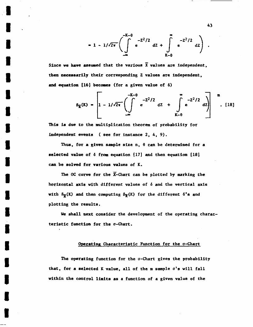
-K-8 m

-z2/2 -z*/2 = 1 - l/G(s e dZ + e dZ) .

-0 K-8

Since we have assumed that t h e various values are independent,

then necessarily the i r corresponding 2 values are independent,

and equation [la] becarses (for a given value of 6) -

-K-8

l- l /&(J e -2212 dZ + e-z212 d~ .. [18]

-OD K-8 - This is due t o the multiplication theorem of probabili ty f o r

independent events ( see for instance 2, 4, 9 ) .

Thus, for a given sample s i z e n, 8 can be determined fo r a

selected value of 6 from equation j171 and then equation (181

can be solved f o r various values of K.

The OC cume f o r the %Chart can be plotted by marking t h e

horizontal axis with different values of 6 and the ve r t i ca l axis

with S-,(K) and then computing &(K) f o r the d i f fe ren t 6's and

plot t ing the resu l t s .

We s h a l l next consider t h e development of the operating charac-

teristic function f o r the u-Chart.

Operating Characterist ic Function fo r the u-Chart

The operating function for the u-Chart gives the probabili ty

that , fo r a selected K value, a l l of the rn sample u's w i l l f a l l

within the control l i m i t s as a function of a given value of the

1 I * I I 1

44

process standard deviation. This value of the process standard

deviation cun be represented by the process standard deviation

under control conditione plus the quantity 6, which now indicates

some shift in this standard deviation. Symbolically we have

uc - u ’ + d 6 where

If we divide both sides of each inequality by u i we obtain

Now the quantity nu2/ug2 is known to be distributed as a chi

square (x2) distribution (4). Therefore,

and equation 1191 becomes (for a given value of 6) m

BU(Q = r p ( LcL,/u6’ < < UqJUgc 1 I

By squaring each side of the Inequality and multiplying through by

n, we finally obtain m

e , ( ~ = P [ (LCL,/ui)2n < x 2 < (ucL,/u;)% I 1 1201

This probability function can be solved for a selected value of K

and u i by integrating the frequency function of the x2 distribution

over the indicated limits. The frequency function of the x2 distribution is given by -

v/2-1 4 / 2 f(X2) = (x 2) e 9

v/2

where v is the number of degrees of freedom given by v = n-1.

45

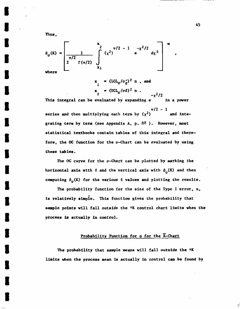
Thus,

r X l m

L where

x = (UCL,/U~)~ n . 2 -x2/2

This in tegra l can be evaluated by expanding e i n a power

VI2 - 1 series and then multiplying each term by (x2) and inte-

grating term by term (see Appendix A, p. 88 ). However, most

statistical textbooks contain tab les of t h i s in tegra l and there-

fore , the OC function f o r the a-Chart can be evaluated by using

these tables.

The OC curve f o r the o-Chart can be plot ted by marking the

horizontal axis with 6 and the v e r t i c a l axis with e,(K) and then

computing B,(K) fo r t h e various 6 values and p lo t t ing the r e s u l t s .

The probabili ty function for the s i z e of the Type I er ror , a,

is re la t ive ly simple. This function gives the probabili ty t h a t *

sample points w i l l f a l l o u t s i d e the *K control chart l i m i t s when the

process is actual ly i n control.

Probabili ty Function f o r a f o r the %Chart

The probabili ty tha t sample means w i l l f a l l outside the *K

l imi t s when the process mean is ac tua l ly i n control can be found by

46

integrat ing the standardized normal equation over the area outside

these l i m i t s .

,

[ dZ ] , ,292 crj?(K) = l/& e dZ +

o r m

or;?(K) = 2/& dZ . J K

Probabili ty Function fo r Q f o r the a-Chart

The probabili ty tha t sample standard deviations w i l l f a l l out-

s ide of the *K l i m i t s when the process standard deviation is actual ly

i n control can be found by integrating the frequency function for

a over the area outside these limits.

Thus, -K W

aa(K) = f(a)da + s f(cr)da ,

-OD K

where f(a)da is defined by equation 171.

Since the d is t r ibu t ion of a is not necessarily symmetrical,

aa(K) cannot be fur ther reduced.

C M P T E R V

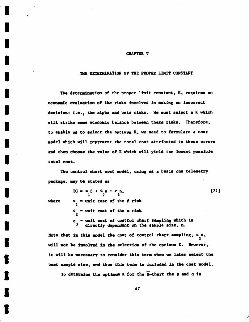
TBE DETESWINATIOIO OF TBE PROPER LIHIT CONSTANT

The de te rdna t i an of the proper l l m i t constant, K, requires an

e c d c evaluation of the risks involved in making an incorrect

decisian: Le., the alpha and beta risks.

will strike some econaric balance between these risks,

W e must select a K which

Therefore,

t o enable us t o select the optimum K, we need t o formulate a cost

d e l which w i l l represent the t o t a l cost a t t r ibu ted t o these e r rors

and then choose the value of K which w i l l yield the lowest possible

t o t a l cost,

The control ch8rt co8t model, using a8 a b a s h one telemetry

package, may be stated an

TC = C 8 + f a + CU, 1 2 3

where c = un i t cost of the 8 r i s k

c - unit cost of the a r i s k 1

2

c = unit cost of control chart sampling which is d i rec t ly dependent on the sample size, n.

Note that in thh d e l t h e cost of control char t sampling, c n, 3

vi11 not be fmolved in the select ion of the opt- K.

it w i l l be neceusary t o canolder th ie term when we later select the

best s q l e 8ite, and thus th i s term is included in the coat d e l .

To detcr r iae the o p t l a m K f o r the --Chart the B .ad a in

Bowever,

47

48

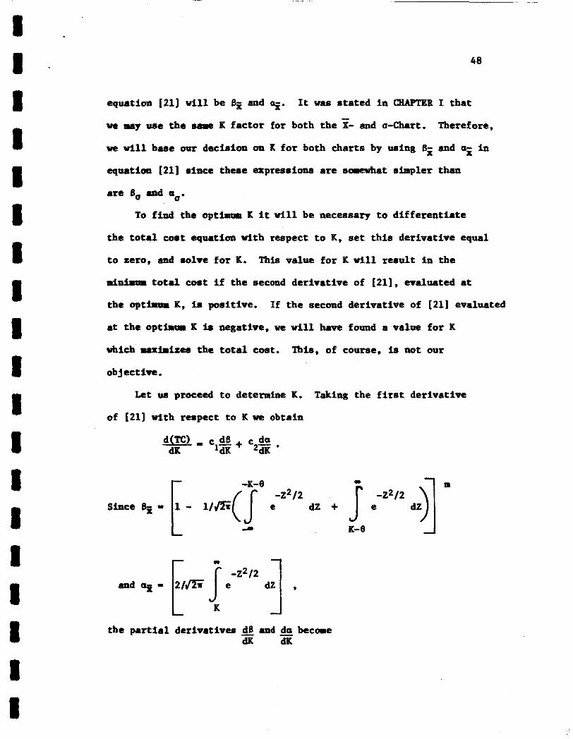
equation (21) w i l l be Sz and q.

we may ode the s u ~ e K fac tor for both the E- and a-Chart.

we will base our decision on K f o r both charts by using 8;; and a;; in

equation (211 since these expressions are s d a t siarpler than

are B,, and a,,.

It was s ta ted in CHAPTER I t ha t

Therefore,

To find the opthum K it w i l l be necessary t o d i f f e ren t i a t e

the tot81 cost equation with respect t o K, set t h i s derivative equal

t o zero, and solve fo r K. This value fo r K w i l l result in the

dnirmr t o t a l cost i f the second der ivat ive of (211, evaluated at

the o p t h a K, I s positive.

at the optirtmr K ir negative, we w i l l have found a value f o r K

which maxirites the t o t a l cost. Thb, of course, is not our

If the second der ivat ive of [21] evaluated

objective.

L e t UII proceed to determine K. Taking the f i r s t der ivat ive

of (21) with respect to K we obtain

a L

t h e partial derivatives a and & become dK dK

1 I -

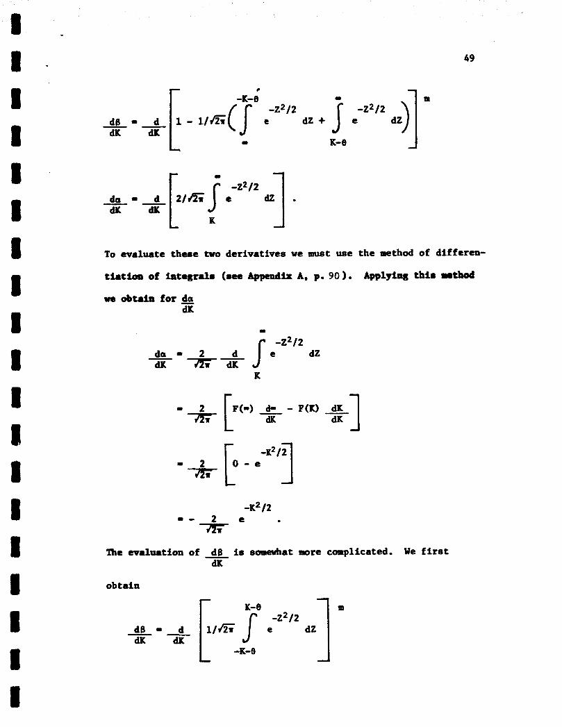
d - - dK

do = d dK dK - -

49

To evaluate these two derivatives we must use the method of diffcren-

thtian of integral8 (me Append* A, p. 90) . Applying thia wthod

ve obtaia for dK

m

-2212 - da - 2 d s e dZ dK 7 E - x

K

r 1

I - 2 I P(-) dm - P(K) dK rrZr dK dK L J

-K2 /2 - - 2 e . rrzI

The evaluation of dB is somewhat more complicated. We first dK

obtain

In order to eliminate the integral

power series and integrate tam by

-2212 sign let us expand e h a

tern.

K-8 It-R -- - -2212

dZ = (1 - - Z2 + Z4 - Z6 + ...) dZ 2 4.21 8.31

4 - 8 -K-8

I = 2 - 23 + z5 - 27 + 0 . . - - - 6 40 336

-K-8

= p-8’ - + (K-8)5 - (K-eJ + 6 40 336

- L 336

1 . u - 8 I I li 8 I 8 1 1 I 1 I I 8 I

51

Pactoris (K4) f r a the first serlcrr a d (-K-e) from the second

*el&

4 - 8 j. -22/2 e d z -

r-

r 1 - (K-6)2 + (K-e)4 - (K I 2.3 4.5-21 8.7.31

L

1

L -1

r-

+ .*I + *.q 1

bracketed expression, the raaini-

e in seriea foxm- Thus,

0

The m a of the serics Z 1/2n is 2; therefore, 2.

I 1 8 1 I I I 1 I 1 1 I II 8 1 I I 8 8

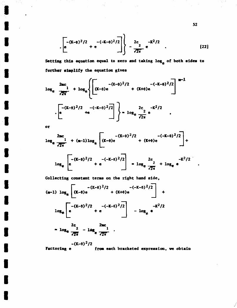
52

Setting this equation equal to zero and taking loge of both sides to

farther simplify the equation gives

-(-K-8)2/2 I+ -(K-6)*/2 (K-elc + (K+e)e c 2rrc

2c -K2/2 '

1-e + e . Collecting constant terms on the right hand side,

-(-K-9)2/2 I + - (K-8) 2/2 (m-1) lag, (K-We + (K+8)e

-K2/2

II -(K-8)2/2 -(-K-8) 2/2 - log e + e 1 e

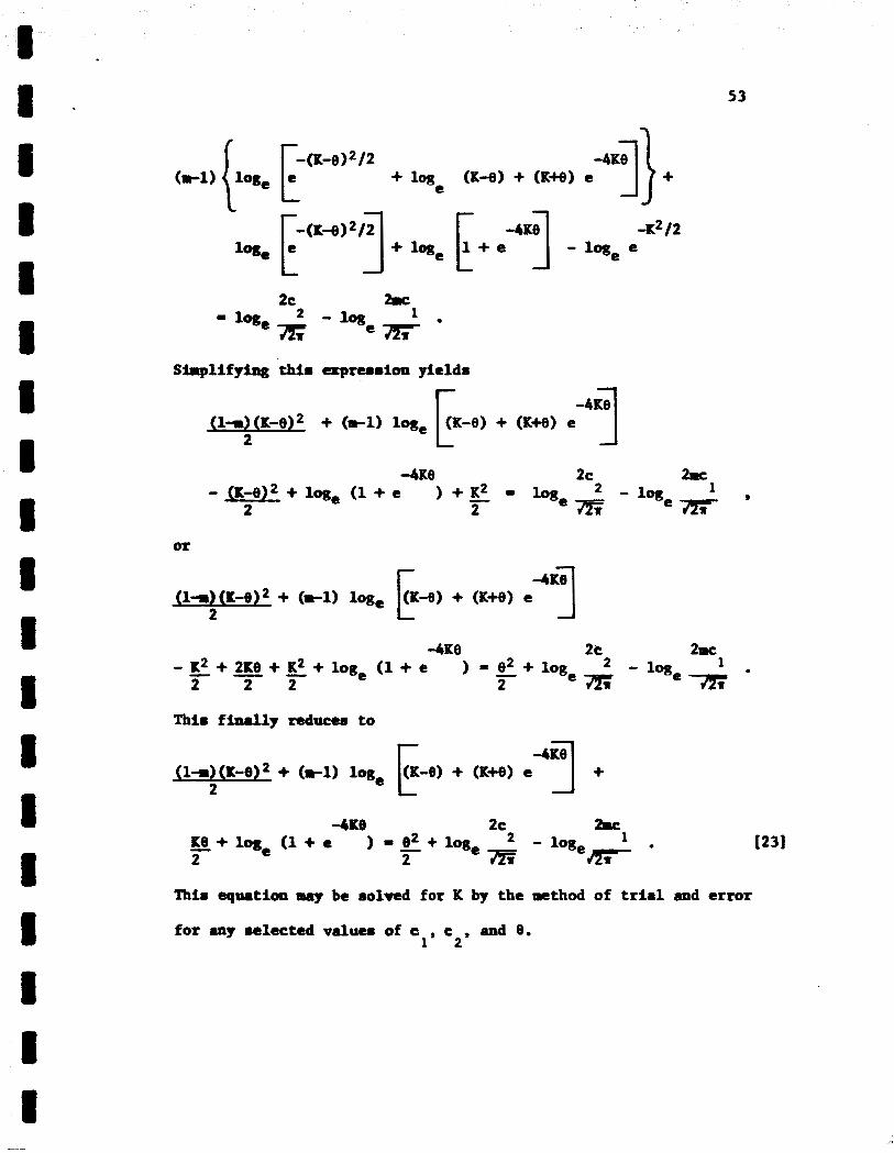
-(K-@) 2/2 Factoring e f r a each bracketed expression, we obtain

53

2c &

Simpllfylng this apressioa y ie lds

-4K8 2c 2n: - (K-8)2 + log, (1 + e ) + e - loge 2 - 1

2 2 7zii

-4K8 2e 2mc 2 - 1

losex . - ~ + ~ + ~ + i o g e ( 1 + e = & + l o g e 2 2 2 2 71;;

T h l m finrrlly reduce6 to

Thls equation rray be solved for K by the method of trial and error

for any 6clectcd valuea of c , c , and 8. 1 2

54

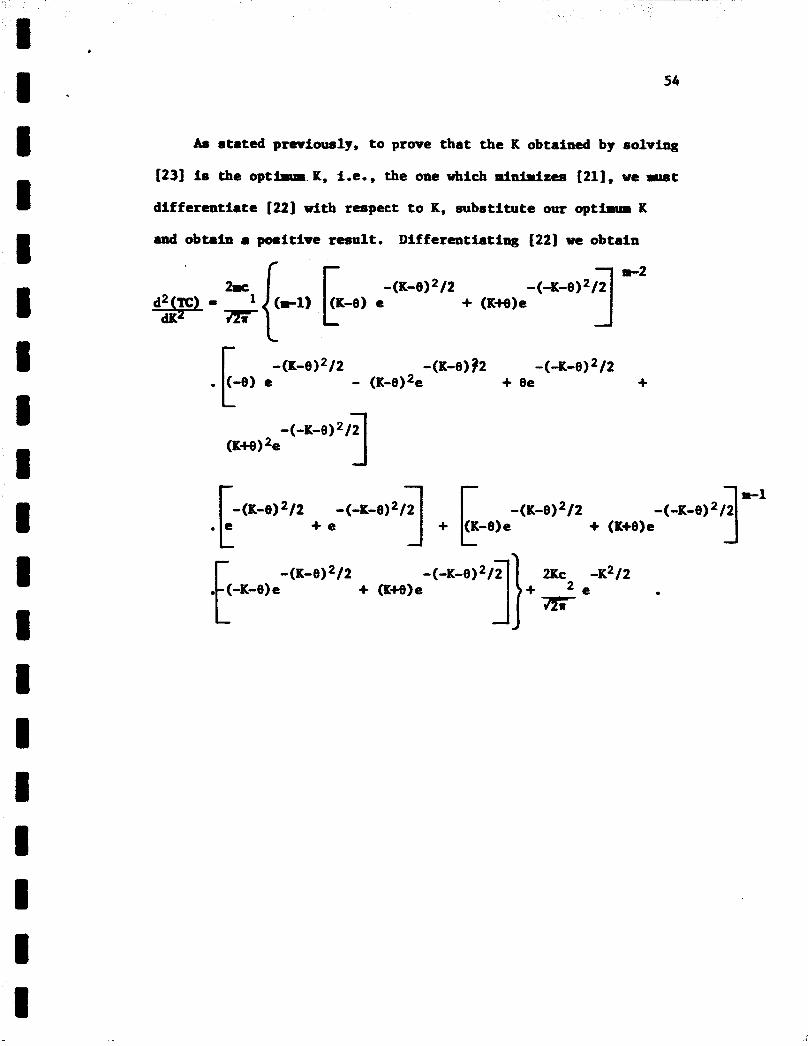
As stated previously, to prove that the K obtained by solving

(231 is the opt-. K, %.e., the one which minimizes (211, we arrrt

differentiate (22) w i t h respect to K, substitute our opt- K

and obtain a positive result. Differentiati- (22) we obtain

-(+e) 2/2 + (K+8)c

- (K-8) /2 -(K-e) 32 - (-K4)2/2 + 0e +

- (-be) 2 /2 1 (KM) 2e

-(-K-e)2/2 I” - (K-e) /2 - (-K-e) /2 -(K-8)2/2 + e + (K+e)e

-(K-8) 2/2 (-K-e)e + (K+e)e F

CHAPTER V I

APPLICATION OF TEE ~ [ B w l u K ; y

The control chart methodology is now completely fonnrlated;

therefore, we may apply the methodology t o a telemetry package

experiment and hopefully obtain meaningful resu l t s .

Description of the Expe rimental Output

The experlmental set-up w a s described in CHAPTER I11 and a

block diagram of the experiment given by Figure 5 .

14 subcarrier o sc i l l a to r s available i n the experimental telemetry

package.

maladjusted SCO's.

w e r e purposely caused t o have higher va r i ab i l i t y than the others

by inject ing random noise into the system through these channels.

This condition would correspond t o a package having two "noisy"

SCO's. These two types of malfunctioning components represent

the conditions fo r which the control char ts have been designed

t o detect . Therefore, i f the methodology has been formulated

correctly, the four SCO's (channels 4, 6, 12, and 13) will be

judged out of control by the control charts.

There w e r e

"bo of these SCO's, channels 4 and 6, w e r e purposely

Also two of the SCO's, channels 12 and 13,

This w i l l , of course,

55

I I I I I 1 I I I 1

56

r e su l t i n a decision t o investigate these SCO's for assignable

causes of var iab i l i ty .

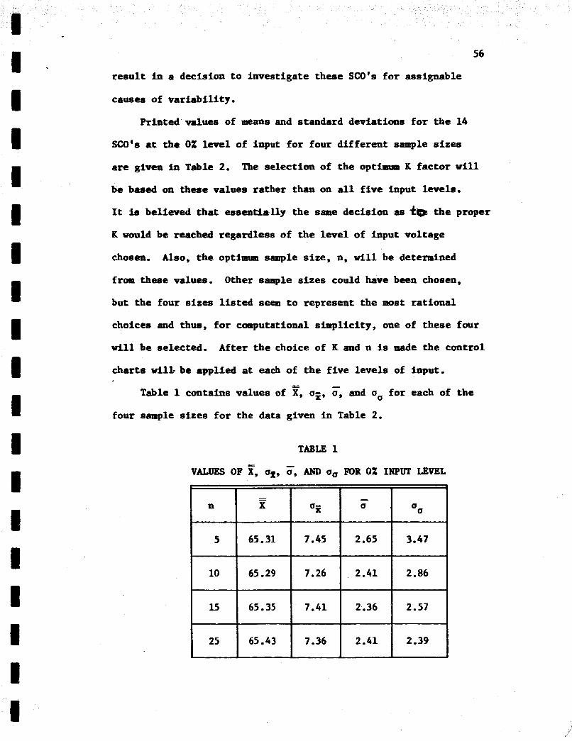
Printed values of means and standard deviations fo r the 14

SCO's at the 0% level of input fo r four d i f fe ren t sample sizes

a re given in Table 2.

be bused on these values rather than on a l l f ive input levels.

It is believed tha t essentirrlly the same decision as

K would be reached regardless of the level of input voltage

chosen. Also, the optimum sample s ize , n, w i l l be determined

from these values.

but the four sizes l i s t e d seem to represent the most ra t iona l

choices and thus, fo r computational simplicity, one of these four

w i l l be selected. After the choice of K and n is made the control

char ts will .bc applied at each of the f ive leve ls of input.

The select ion of the optimum K fac tor w i l l

the proper

Other sample s i zes could have been chosen,

Table 1 contains values of z, uz, F, and uu for each of the

four sample sizes fo r the data given in Table 2.

TABLE 1

VALUES OF E, ur, u, AND ug FOR 0% INPUT LEVEL -

w 0

57

58

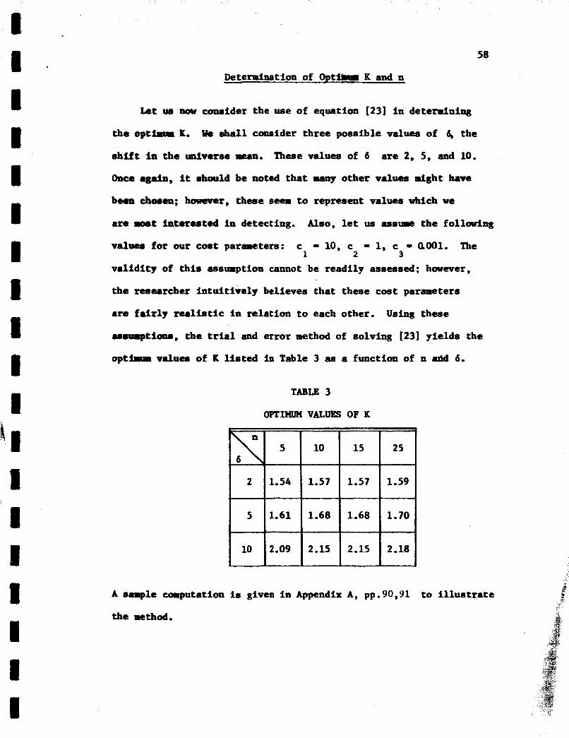
Deteraination of Opt- K and n

Let tm PQV consider the use of equation (23) i n determining

the opt- IC. We shall consider three possible valuem of 4 the

s h i f t in the @verse mean. These values of 6 are 2, 5, and 10,

Once -.in, it should be noted tha t m8ny other values d g h t have

been choam; however, theme seem t o represent values which w e

are m t Interested i n detecting. Also, le t us assume the fol lmdng

valuee for our cost parameters: c = 10, c = 1, c - 0001, The

va l id i ty of t h i s assumption cannot be readily assessed; havever, 1 2 3

the researcher i n tu i t i ve ly believes tha t these cost parameters

are f a i r l y realistic i n re la t ion t o each other.

ummptionm, the t r ia l and error method of solving (231 yie lds the

opthum values of K l i s t e d in Table 3 as a function of n abd 6.

Using these

TABLE 3

O P T M u n VALUES OF K

A sample c a p u t a t i o n is given i n Appendix A, pp.90,Yl

the method,

t o i l l u s t r a t e

59

Table 4 gives values of total cost, deterrined from equation

[21], f o r t he a n s w d cost parameters.

5

2 1.4576

5 0.8614

10 0.58%

TABLE 4

VALUES OF TOTAL COST (TC - c B + c a + c n) 1 2 3

10 15 25

1.5074 1.5124 1.5224

1.1070 1.1120 1.1220

0.7586 0.7636 0.7736

It can be seen from Table 4 tha t the optimum sample site

( the value of n which results in the laininnan total cost) is

n = 5 regardless of the site s h i f t i n t he universe mean tha t w e

wish to detect.

based on a sample s i z e of n - 5 for the other four levels of

voltage input.

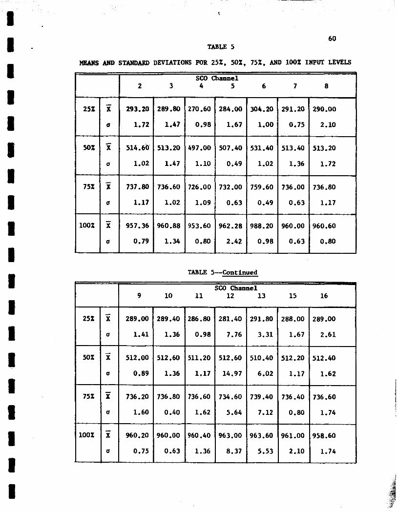
Thus, Table 5 giveim means and standard deviations

Before applying the control char ts t o the f ive levels of

input we must decide on the amount of s h i f t i n t he m e a n we wish t o

detect since d i f fe ren t values of 6 const i tute d i f fe ren t values of K.

Let us assume t ha t w e are most concerned in detecting s h i f t s of

site 6 = 5.

is K - 1.61.

Under this assumption, the optimum K given i n Table 3

Analysis by Control Charts

W e first analyze the data given given i n Table 2 fo r n - 5 for

25%

50%

75%

100%

- X

U

51

U

x U

- x

U

291.20

0.75

513.40

1.36

736.00

0.63

~ 960.00

~ 0.63

290.00

2.10

513.20

1.72

736.80

1.17

960.60

0.80

- 25% X

U

50%

U

- 75% X

(I

- 100% X

U

289.00

1.41

512.00

0.89

736.20

1.60

960.20

0.75

t 1 I - I 1 I 0 I I I I t ff P 1 1 1 1 1 1

60 TABLE 5

PiEANS AND STANDARD DEVIATIONS FOR 25%, 50%, 75%, AND 100% INPUT LEVELS

SCO Channel 1 2 3 4 5 6

~~ ~~

293.20

1.72

289 -80

1.47

514 . 60' 1.02

497.00 507.40 531.40 I I S13 . 20 1.47 1.10 0.49

732 .OO

0 -63

1.02

759 . 60 0.49

988 . 20 0.98

737 . 80

1.17

736.60

1.02

726 -00

1.09

953.60

0.80

957.36

0.79

962 . 28 2.42

960.88

1.34

TABLE 5-Continued -d I SCO Channel

16 I ' 11 15 10

289 . 40 1.36

512 -60

1.36

736 . 80 0.40

12 13

286.80

0 -98

511 . 20 1.17

289 -00

2.61

288 . 00 1.67

512.20

1.17

- 512.40

1.62

736 -60

1.74

958.60

1.74

736.60

1.62

734 -60

5 -64

739.40

7.12

736 . 40 0.80

961.00

2 .lo

960 -00

0.63

960 -40

1.36

963.00

8.37

963.60

5 -53

61

v a r i a b i l i t y by the use of the u-Chart.

and ug - 3.47.

center l i n e become

From Table 2, a = 2.65

Thus, with K = 1.61, our control limits and

The

are

and

a-Chart is given

out of control,

both t h e i r and -

- UCL - u + - 2.65 + (1.61)(3,47)

= 5-59

L c L = u - -

&a

= 2.65 - (1.61)(3.47) - 0 , since negative -

C+, = u = 2.65

i n Figure 11, (a). SCO channels 12 and 13

Therefore, these SCO's require investigation

u values are eliminated from the data. Re-

computing 0 and u,, w e have - u = 1.39

uu = 0.37

Thw, our revised l i m i t s and center l i n e become

UCL - 1.99

CL - 1.39

LCL = 0.79

We now observe from Figure 11, (b) t ha t channel 16 is out of control.

Once again, we eliminate

lwts and center l ine.

the data fo r t h i s channel and revise our

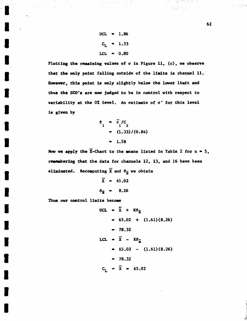
62

UCL - 1.86

C+, - 1.33

LCL - 0.80

Plot t ing the remaining values of u i n Figure 11, ( c ) , w e obseme

tha t the only point f a l l i n g outside of t he limits is channel 11.

€lowever, thia point ie d y s l igh t ly below the lawer l i m i t and

t h w the SCQ'r are pov judged t o be i n control with respect t o

var i ab i l i t y at the 0% level. An estimate of uc for t h i s l eve l

is given by -

e - o / c 1 1 2 - (1.33)/(0.84)

Nov we apply the &chart to the means listed in Table 2 f o r n = 5 ,

r e r a b c r i n g tha t t he data for channels 12, 13, and 16 have been

eliminated. Recomputing and 6~ we obtain - - X = 65.02

bji 8.26

Thus our control l i m i t s become - -

UCL X + Kbji

= 65.02 + (1.61)(8.26)

= 78.32 - -

LCL = x - Keg

= 65.02 - (1.61)(8.26)

* 78.32

63

UCL - 5.59 --e - - - - - --- -- - -- 6.00 9

5.00 - 4:Oo -

CL - 2.65 (a)

v LCL - 0 2 3 4 5 6 7 8 9 10 1112 13 15 16

SCO Channel

2.25 - 2.00:

0

y1 0

m u C 3

UCL = 1.99 --e- ---e--

4 1.75

Q Q) (b) 1.50 CL = 1.39 a 1.25 - u bl

r( 8 u

1.00 t -------- - -e-- LCL = 0.79 3 2 1 1 1 1 1 1 1 1 1 1 1 2 3 4 5 6 7 8 910111516

SCO Channel

2 3 4 5 6 7 8 9101115 SCO Channel

FIGURE 11. CONTROL CHARS FOR u, 0% INPUT Data from Table 1, n = 5. (a) gives or%ginal chart. (b) and (c) are revised charts.

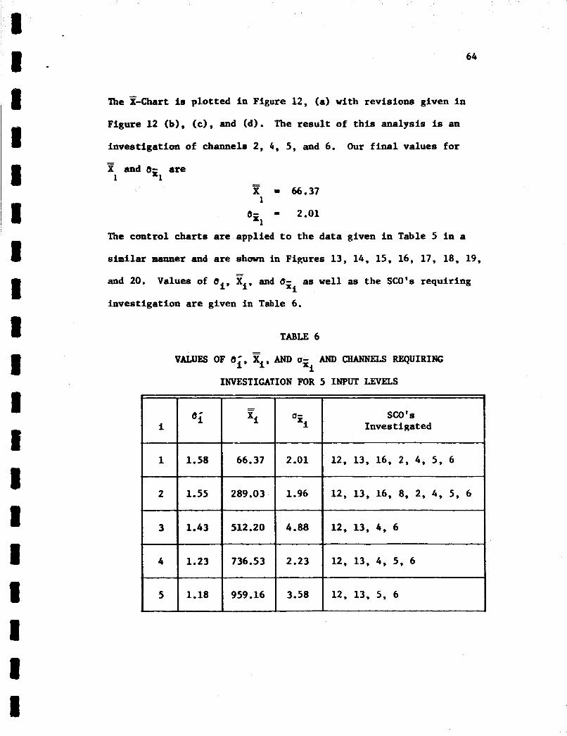
64

1 I - -

U- SCO'S =i Investigated ei xi

i

The --Chart is plotted i n Figure 12, (a) with revisions given i n

Figure 12 (b), (c), and (d). The re su l t of t h i s analysis is an

investigation of channels 2, 4, 5 , and 6.

X and 8- are

Our f i n a l values fo r =

- - 1 =1

X = 66.37

e- - 2.01

The control charts are applied t o the data given i n Table 5 i n a

1

=1

similar manner and are shown in Figures 13, 14, 15, 16, 17, 18, 19,

and 20. xi

- - Values of bi, Xi, and 8- as w e l l as the SCO's requiring

investigation are given i n Table 6,

TABLE 6 =

VALUES OF e;, Xi, AND U- AND QIANNELS REQUIRING xi

INVESTIGATION FOR 5 INPUT LEVELS

65

,a \ t/

Y

2 3 4 5 6 7 8 9 1 0 1 1 1 5 SCO Channel

75 -. - - - - - -- - UCL = 73.95

70 65 k k , CL = 67.32

2 3 5 6 7 8 9 1 0 1 1 1 5 SCO Channel

2 3 5 7 8 9 1 0 1 1 1 5 SCO Channel

70 L UCL = 69.61 ------------

CL I 66.37

6o t 1 1 1 1 1 1 1 1

3 7 8 9 10 11 15 SCO Channel

FIGURE 12. COhTROL CHARTS FOR E, 0% IXPL!. Data from Table 1, n = 5 . (a) gives or i f f ina l chart. (b), ( c ) , and (d) are revised charts.

5.60 4.00

(a) 3.'' 2.00

1.00

3.00

(b) 2*oo

1.00

0

cec 0

(R U

3.00

rl G J

'd

2.00

u ( c ) 1.00

66

= 4.81

= 2 . h

- 0

t - - UCL 2.71

- - - _. - - _. - - - - LCL = ..).53 l l l l l l l i l l l l l

2 3 4 5 6 7 8 9 1 0 1 1 1 3 1 5 1 6 SCO Channel t

= 1.48

LCL - 0.b7 ---------- 2 3 4 5 6 7 8 9 1 0 1 1 1 5 1 6

SCO Channel

_. - - - - UCL - 2.01 -k 2.00 - - -

SCO Channel FIGURE 13. COITROL CHARTS FOR Q, 25% IXPL'T.

Data from Table 5. (a) Rives oripinal chart. (b) , ( c ) , id) , and (e) are revised charts.

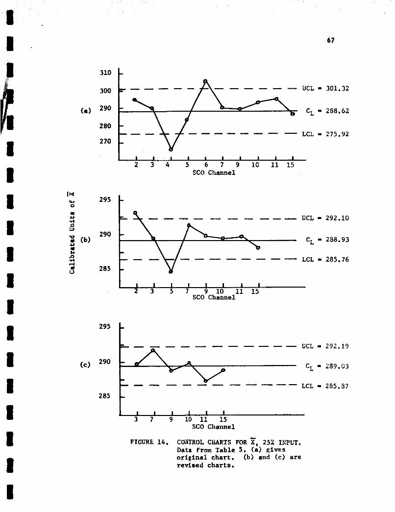
67

295

290 (e)

285

310 - 300

290 7

280 - 270 -

UCL - 301.32 - - - - - CL I) 288.62 (a)

LCL - 275.92 --- - - - - - - - -

1 I I I I I 1 I I I 2 3 4 5 6 7 9 10 1 1 1 5

SCO Channel

- UCL - 292.13 & - - - - - - - ----

A CL = 289.03 - .-

LCL - 285.37 - - - - - - - ---- -

1 I I I I I

I I I I I I I 1 I 2 3 5 7 9 10 11 15

SCO Channel

FIGURE 14. COiVTROL CHARTS FOR ?I, 252 ISPUT. Data from Table 5 . (a) gives original chart. (b) and (e> are revised charts .

8 1

1 1 1 1 1 1 1 1 1 1 1 1

68

10 . 00 8.00

6.00

4.00

(a)

2.00

- - - - - - - - - - - - -

cL

LCL 5 6 7 8 9 10 11 12 13 15 16

SCO Channel 2 3 4

= 3.45

= L.53

- 0

0 4.00 I)

UCL = 3.70 _ - - - - - - - --- u-c 0

m U .d E: ;>

3.00 - a 9) 2.00 - ; (b) CL = 1.57 h 0 r( r( d U

1 1 1 1 1 1 1 l l l l l l 2 3 4 5 6 7 8 9 10 1113 15 15

LCL = 0

SCO Channel

FIGURL 15. CONTROL CHARTS FOR (3, 50% IXPUT. Data from Table 5 . (a) r i v e s oripinal chart. (b) and (c) are revised charts.

525

520

515

(a) 510

505

500 Ix yc 0

m U 2 5

525

520

515

510

505

500

IrrJ I I I I I I I I 2 3 4 5 6 7 8 9 1 0 1 1 1 5 1 6

SCO Channel

69

UCL = 524.24

Ct = 512.55

LCL - 500.56

-- I f..,..... SCO Channel

FIGURE 16. COh'TROL CHARTS FOR ?I, 502 IXPUT. Data from Table 5. (a) gives oripinal chart. (b) is the revised chart.

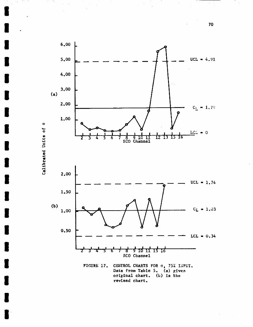
70 R .

LCL - - - - - - - - - - - 1 1 1 1 1 1 1 1 1 1 1 1

6.00

5.00

4.00

2.00

1.00 b

YI 0

(D u 4 C 3 ‘FI PI 4J * Lc

4 cd 3 V 2.00

1.50

(b 1 1.00

0.50

UCL

CL

FIGURE 17. CONTROL CHARTS FOR 6, 752 ISPUT. Data from Table 5 . (a) gives original chart. (b) is the revised chart.

= 4.91

= 1.74

= 1.33

- 0.34

71

- - - - - - - - - - - UCL 749.13 750 .. 745 - 740 -

CL 737.20 (a) 735 L a

730 - 725 c

I I I I 1 I I I I 1 I I I 2 3 4 5 6 7 8 9 1 0 1 1 1 5 1 6 I SCO Channel

I 740 UCL - 741.49 - - - - - - - - - - -

740

(d) 735

I I I I I: I 8

- - - - - - - - - - UCL - 740.12 - -

V d CL 736.53 - - - - - - - - - -

CL - 735.1C

- - - - - - -- LCL - 723.83

(b) 735

730

725 IX (u .. 0

0 U 4 G 3

I I I I I I 2 3 4 5 7 8 9 1 0 1 1 1 5 1 6

SCO Channel

FIGURE 18. COHTROL CHARTS FOR z, 752 IKPUT. Data from Table 5. (a) gives original chart. (b), (c), and (d) are revised charts.

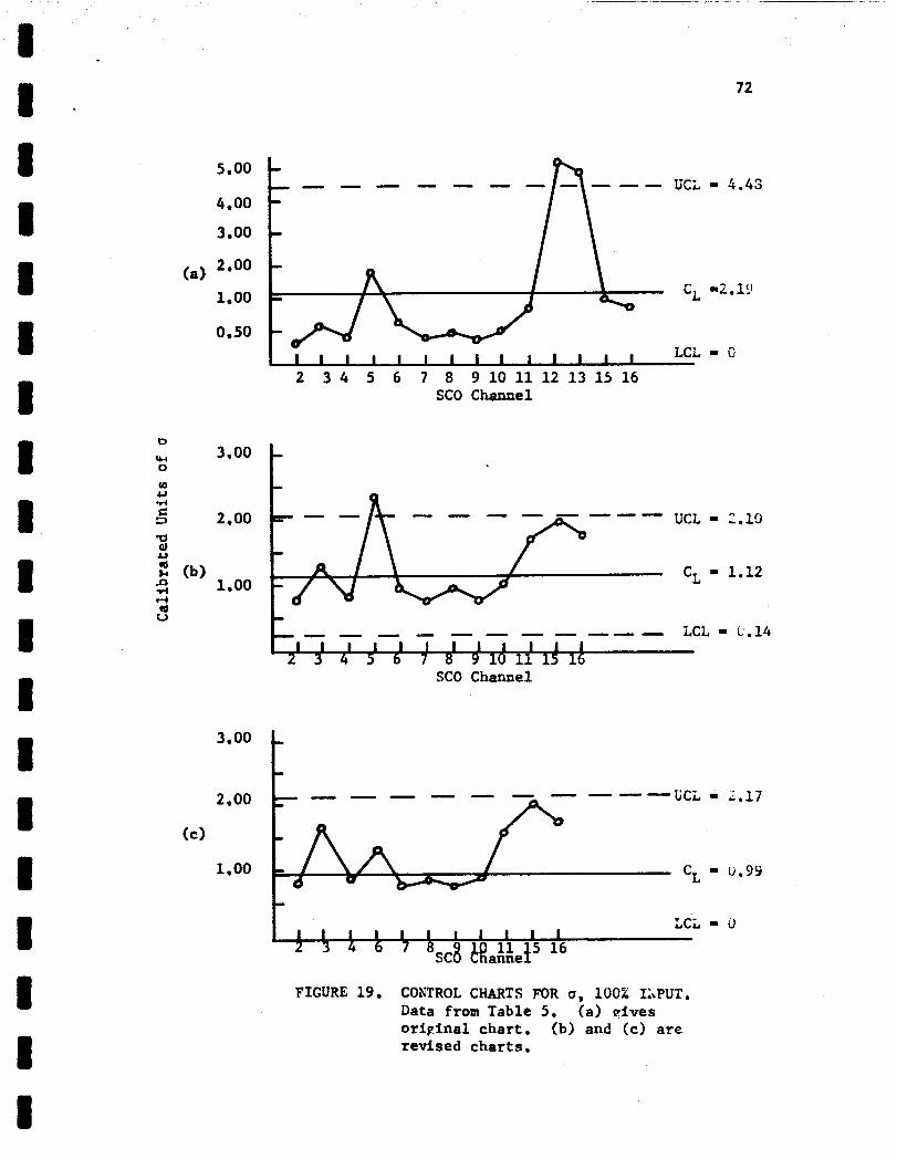
5.00

(a) 2*oo 1.00

0.50

72

- 4 . 4 3

2 3 4 5 6 7 8 9 1 0 1 1 1 2 1 3 1 5 1 6 SCO Channel

FIGURE 19. CONTROL CHARTS FOR U, 100% ILPUT. Data from Table 5 . (a) aives oripinal chart. (b) and ( c ) are revised charts.

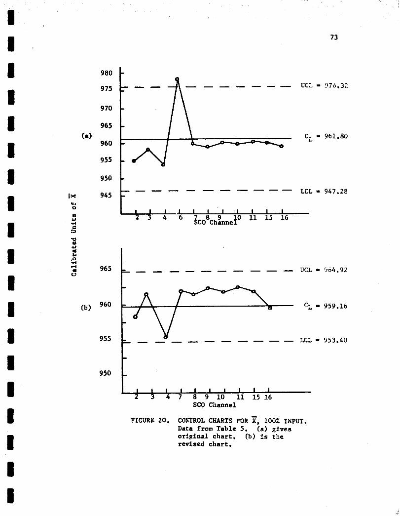
Ix # 0

U a

950

r( 0 3

- - - - - - - - - - - LCL 953.4G

- -

I I I I I I I I I I

m U U a Lc

rl a u

3

73

975

970

965

960

955

UCL - 376.32

CL - 961.80

FIGURE 20. COhTROL CHARTS FOR y, 100% INPUT. Data from Table 5 . (a) gives original chart. (b) i s the revised chart.

II I I

74

The best estimates for the population standard deviation

at each voltage input level were given in Table 6. Therefore,

we may estimate the universe standard deviation for the telemetry

package as

5 %

0’ - i=l 5 - (1.58 + 1.55 + ... + 1.18)

5

= 1.39

Previous work has shown that a measure of telemetry system precision

(random error) is given by the standard deviation expressed as a

percentage of the range9 of the process, u

Thus, we may estimate the precision of the telemetry package that

- lOOo/E (5). P

we have analyzed as

where

Obtaining and zdn from Table 6, lLlx -

R = 959.16 - 66.37

= 892.79 . Our estimate of the precision now becomes

u = lOO(1.39) P 892.79

= 0.16%

’The range is merely the difference in the highest and lowest values.

I - 75

1 I I 8 I I 1 I I I 1 I I 1 1

Further work (6) has established that a measure of telemetry system

accuracy (systematic errors) is given by

where 4 ie a variance of t h e mean values about a theoretical

curve f i t t e d to the data, or

h c (4 - ip

q$ = 111 h - r - 1

A

In the equation Pi is the theoret ical ordinate from the curve

which bes t fits the 4 points and r is the degree of t h i s curve.

A regression unalysis was performed vith the a id of the

University of Alabama Univac SS 80 computer and a linear equation

was found to provide the best f i t t o the data,

coefficient (degree of relationship) f o r the l i nea r f i t was 0,99799.

Using t h e theoret ical ordinates obtained from the l i nea r equation

The correlat ion

the variance of the mean values about the curve w a s found to be

4 = 1648.21 . Thus our estlmate of the accuracy of the telemetry package becomes

= 100 J(1648.21 - (1.39) /(14)(5) 892.79 ‘a

- 100 rh646.28/70 892.79

* 0.54% . Expressed as 99% confidence l i m i t s the values of accuracy and

precision are

Average Precision = 0.48%

Average Accuracy - 1.62% .

76

This may be interpreted as meaning tha t w e would be approximately

99% cer ta in tha t t he precisian of t he telemetry package tha t we

have analyzed is no worse than 0.48% and tha t the accuracy is no

worse than 1.62%.

We MY llc~v set standards fo r future control chart analysis

of telemetry systems (based on n = 5* 6 = 5 ) .

For the a-Chart, at a l l 5 levels of input,

(+, - C 8 ’ - (0.84)(1.39) = 1.17 2

2

2

UCL = C 8 ’ + KuG - 1.17 + (1.61)(0.42) = 1.85

LCL = c e - - ~ b ; . = 1.17 - (1.61)(0.42) 0.49

where, as implied i n CHAPTER III* equation 1141,

- 0.42 . For the %Chart, at each Input leve l separately,

- - 0% Level: % - X = 66.37

1 =

UCL X + Kby = 66.37 + (1.61)(2.01) 69.61

LCL X - Kbx 66.37 - (1.61)(2.01) 63.13 1 1

1 1

- -

- - 25% Level: CL - X = 289.03

2 - __ UCL X +Kdx = 289.03 + (1.61)(1.96) 292.19

LCL X -K8- 289.03 - (1.61)(1.96) 285.87 2 2 - - 2 x2 I

50% Level: = X = 512.20 3

3 3

3 3

- - UCL X +Kbz 1 512.20 + (1,61)(4.88) 520.06

LCL X - K6x 512.20 - (1.61)(4.88) 504.34 - -

77

- - 75% Level: % = X = 736.53

4

4 4

- - UCL * X + K6x 736.53 + (1.61)(2.23) = 740.12

736.53 - (1.61)(2.23) = 732.94 - -

= 4 -=l( - - 100% Level: % = X = 959.16

5

5 5

5 5

- - UCL X +K8x 959.16 + (1.61)(3.58) 964.92

LCL X - K6x 959.16 - (1.61)(3.58) 953.40 - -

A f i n a l area of i n t e re s t i n applying the methodology w i l l be to

give the OC curves f o r the control char ts based on the standard values

tha t w e have derived.

The OC function fo r the %Chart based on standard values is the

same as tha t f o r past values except tha t the fac tor m i n the

exponent is eliminated since w e are nov interested i n the proba-

b i l i t y of each new saaple z v a l u e f a l l i n g within the limits as they

a r e computed. The function can thus be s ta ted as

r -K-8 1

K-8

Applying t h i s function t o t h e 0% l eve l of input (n = 5, K = 1.61,

8% = 2-01), the OC curve given i n Figure 21 may be derived f o r

various values of 6 (e = 6/6,).

The OC function f o r the +Chart based on standard values may

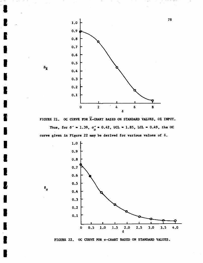
c -

I I t E E 1 T li I t R c 1 I I 1 8

78 1.0 c 0.9

0.8

0.7

0.6

0.5

0.4

0 .3

0.2

0 .1

0 2 4 6 8 6

FIGURE 21. OC CURVE FOR%CHART BASED ON STANDARD V A L W , 0% INPUT.

Thus, for 6’ - 1.39, u.9 0 .42 , UCL - 1.85, LCL - 0.49, the OC U

curve given i n Figure 22 may be derived for various values of 6 .

0.9 loo 1 0.8 t 0.7

0.6

0.5

0.4

0.3

0.2

0 .1

0 0.5 1.0 1.5 2.0 2.5 3.0 3.5 4.0 6

FIGURE 22. OC CURVE FOR U-CHART BASED ON STANDARD VALUES.

CHAPTER VI1

CONCLUSION

This thesis has presented a methodology for determining

whether a telemetry package is in a state of statistical control.

The development of the methodology has required research and

experimentation in the following areas:

1. The theoretical foundation for the establishment of the and u charts;

2. The investigation of the operating characteristics of the ?I and u charts based on past data:

3. The determination of the proper control limit constant, K, from an analysis of a control chart cost model;

4. The determination of the accuracy and precision of the analyzed telemetry system.

This research and experimentation has resulted in the estab-

lishment of a control chart methodology for analyzing past telemetry

system performance and also the specification of control charts

for future analysis of telemetry systems. On the basis of the

control chart analysis, the accuracy and precision of telemetry

systems can be estimated.

The results obtained in CHAPTER VI for the particular telemetry

79

80

package tha t w a s analyzed are suanarized for c la r i ty as follows:

1. Combined use of the x and u charts (considering a l l f i v e

levels of input voltage) resul ted i n the investigation of

SCO channels 2, 4, 5 , 6 , 8, 12, 13, and 16. Of these

eight SCO's, only channels 4, 6, 12, and 13 w e r e del iberately

caused to malfunction.

detected incorrect ly (due t o the alpha e r ro r ) o r w e r e i n

need of investigation due t o assignable causes not

immediately known.

The remaining channels w e r e e i t h e r

2, E s t i m a t e s of the system accuracy and precision, expressed

as 99% confidence l i m i t s , w e r e found to be

Average Precision - 0,48%

Average Accuracy - 1.62% . 3. Standards f o r future control chart analysis w e r e estab-

l ished at a l l 5 levels of input. Selecting only the 0%

l eve l of input as a basis the standards are

u-Chart : UCL = 1.85

% = 1.17

LCL = 0.49

X-Chart : UCL = 69.61 -

- 66.37

LCL - 63.13

cL

4. The OC curves for both the and u charts based on standard

values w e r e given i n Figures 2 1 and 22. The OC curves f o r

81

both charts proved that f o r s h i f t s of 5 o r more in the

universe parameter (? o r a') the probabili ty of not detect-

ing t h i s s h i f t , 8, is ra ther s m a l l . These curves and both

control charts vere based on a K fac tor of 1.61 which vas

discovered to be the optimum K.

Sources of Possible Error

Perhaps the most important assumption in the development of the

methodology is t ha t the individual values of output are normally

dis t r ibuted. This assumption has been made in other reports (5 .6)

although the data was often found to be only moderately normal. The

more non-normal the telemetry data actual ly is, the more w i l l be the

error in u t i l i z i n g the control char t methodology, or f o r t h a t matter,

any other type of parametriclo statistical test.

Another source of possible e r r o r is i n the assumed values of

We have assumed tha t the cost of the beta e r ro r is c lv = 2 ' and 3

t en times as much as the cost of the alpha e r ror , and the cost of the

alpha error is 1000 times as much as the cost of control char t sampling.

Since in the telemetry environment the cost of l e t t i n g defective

components pass inspection is much greater than is the cost of

investigating sa t i s fac tory components, these cost estimates appear t o

be roughly accurate in t h e i r re la t ionship t o each other. Hwever,

i f they are grossly inaccurate, t he select ion of K, t he select ion of

'"Non-parametric tests are not affected by the assumption of normality. See, f o r example, (7).

82

the optimum sample s i z e n, and consequently the development of the

control chart l i m i t s must be made based on t h e new estimates.

these old cost estimates are used (resul t ing i n K - 1.61, n = 5 ,

etc.), and new estimates actually should be made, then some amaunt of

error w i l l be entered in to the analysis.

selected a s h i f t of 6 - 5 as that which w e wish t o detect. I f t h i s

assumption is not val id , our analysis rust be made based on some

other value of 6, and thus a possible source of e r ror might be eli-

minated.

rf

Furthermore, we have

A f i n a l e r r o r source is in the assumption tha t the K factor

selected fo r the F-chart w i l l be sa t i s fac tory f o r the u-Chart.

Sh i f t s i n

fac tor for the determination of K for the %Chart.

wish t o make our analysis more precise by basing the determination

of t he control l imi t s f o r t he u-Chart on some other value of K,

o r perhaps on a K determined for both 2 and u* sh i f t i ng simultan-

eously ( see p. 83).

f o r both charts based on an analysis of the e r rors associated with

the %Chart may have introduced some amount of error .

of 6 - 5 seem to be f a i r l y r e a l i s t i c as a gwerning

However, we may

Therefore, the select ion of one value of K

Recae#ndatians for Future Research and Application

The researcher f e e l s tha t t he methodology presented i n t h i s

thes i s could eas i ly be used t o form the basis fo r a complete tele-

metry package checkout procedure. Once the necessary experimental

83

equipment w a s set up, the actual implementation of the methodology

would become a simple matter.

equipment i n the telemetry ground s t a t ion fur ther enhances the

The use of the SEL data reduction

poss ib i l i ty of t h i s type of analysis.

be p r o g r d t o give means and standard deviations f o r samples of

size n - 5 , 10, 15, etc., these values could be plotted quickly on

control char ts whose l i m i t s w e r e already set and components which

w e r e not i n statistical control could be adjusted rapidly o r could

be immediately replaced.

I f t he SEL equipment could

T h i s thes i s has also suggested a major area fo r future statis-

tical research.

base the determination of t he optimrrm value of K on the assumption

tha t both ? and uc way s h i f t simultaneously.

the investigation of the OC function fo r the control char ts when

both parameters are subject t o simultaneous shif t ing.

of the OC function fo r t h i s s i tuat ion has been accomplished when the

charts are t o be based on standard values f o r future production

(2, 4).

has been made of t h i s function when the charts are based on past data.

The function would take t h e form of a surface and would seem t o be

extremely complicated, yet t h i s would no doubt be a major contribution

t o the f i e l d of m a t h a t i c a l and applied statistics.

As was mentioned previously, it may be desirable t o

This would require

The development

Bowever, as f a r as t h i s researcher knows, no investigation

Another area f o r s t a t i s t i c a l research would be i n a sens i t i v i ty

analysis of the control chart methodology t o the assumption of normality.

A s igni f icant contribution could be made i f a non-parametric method

84

could be found fo r analyzing product va r i ab i l i t y based on dis t r ibut ions

whose form is unknown.

A f i n a l possible area for research and application i n the

telemetry environment is i n t h e use of the control chart methodology

during an actual f l i g h t cal ibrat ion period.

CHAPTER I, the analysis by s t a t i s t i c a l methods of in-fl ight calibra-

t ion data would be a considerable a id i n determining whether the

telemetry package w a s performing sa t i s f ac to r i ly i n t h i s phase. I f

a par t icu lar S U I w a s found t o be out of control, adjustments could

possibly be made f o r t h i s malfunctioning component and ra ther than

completely losing the data from t h i s par t icu lar channel, only a short

t i m e period would be required fo r correcting the component.

As w a s suggested i n

APPENDICES

i

APPENDIX A

MISCELLANEOUS PROOFS, THwIREH3, AND

SAMPLE CALCULATIONS

HISCEUANEOUS PROOFS, THEOREMS, AND

SAMPLE CALCULATIONS

1. Elementary theorems of expectation.

E(c) = C

E(cx) = cE(x)

E(x) = X -

E (x * Y) - E(x) E(y)

E(Ex) = CE(x)

Cc = nc,

where c is a constant and x and y are variables . - iec

-1/2 [ ( j f - X) /a% 12 2. Proof that T* e d z = 0.9973

= x-3":

Let 2 = (z - z)/uz , then dZ = dK/ar and

3 -22/2

dZ = 2/& dZ. -z2/2

-3 0

The value of t h i s las t integral mult ipl ied by the factor 1/&

may be found in most s t a t i s t i c a l textbooks, for instance (9) , to be

07

88

0,49863. Therefore, the value of the given in tegra l is 2(0.49865) - 0.9973. -z2/2

The function f(Z) = (1/&)e is known as t he standardized

normal equation and has a mean of 0 and a variance of 1.

3, Definition of t h e gaaera function, r[(n-1)/2] ,

s k -v

0 k -V k-1 -V

By def in i t ion r (K) - V e dV . Let U = v , dv = e dv, dU = kv dv, V = -e and

Qo

k-1 -V C(K + 1) = -v Ir-" e I

0 0 - 1 kv (-e! d v )

= 0 - 0 + W ( K ) , by the method of integration by parts .

When w e have a posi t ive integer m for the argument of the

function, repeated use of the above equation yields

r(m) = (m - 111 r(1).

m is not an integer, such as r[(n-i)/21, ve muat use

logarithms and tables of fac tor ia l s .

are used fo r the last factor.

4. Developgent of method for evaluating

89

where X = (Ln/ui)2n, and 1

2 x = (ucL/ui)2n .

L e t x2 = y to simplify the expression.

X X ._

v/2 - 1 -y/2 VI2 - 1 e d l = / b

0 0

ml2 - n - - + J - Y + 0 . . + y dy 1 - 1 w-2 9-2 3v/2 - 3

2 4 12 2 4 0

X k+l kv/2 - k

= 1 j (-1) J k-1 2*k!

0

r kv/2 - k + 1 1

A similar r e s u l t is obtained for

X VI2 - 1 -y/2

e dY

0

90

5. Method of Differentiation of integrals (12, 14).

The fundamental theorem of integral calculus states that

whenever f(x) is a continuous function in the closed interval

(a, b) and F(x) is a function such that P’(x) - f(x), then

U

f’ f(k) dX = F(uI) - P(u 1 0

U 0

for any two points u and u in the interval. If u and u ,o 1 0 1

are differentiable function of another variable, y, so that

the right hand member in the above integral is a function of

y and the chain rule of differentiation gives

Since a similar result holds for F(u ), differentiation of

The original integral yields 0

6. Sample calculations for finding optimum K from equation f23)

by trial and error.

Assume n = 5, m = 14, c, = 10, ct - 1, 8j; = 7.45, O = 0.67.

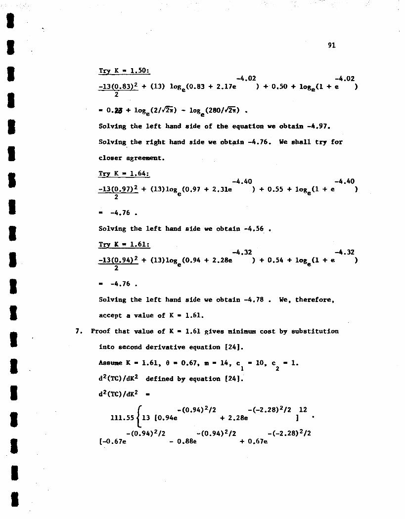
8 . 8 - 8 I I II I I I 8 8 S I * I - I 8 8 I

Try K = 1.50: -4.02

91

-4.02 -13(0,83)2 + (13) loge(0.83 + 2.17e ) + 0.50 + loge(l + e )

2

= 0.w + l0ge(2/&) - log (280/&) . e

Solving the lef t hand side of the equation we obtain -4.97.

Solving the r igh t hand side w e obtain -4.76. W e s h a l l t r y for

closer agreement.

Try K = 1.64: -4.40 -4.40

-13(0.97)2 + (13)log (0.97 + 2.31e ) + 0.55 + loge(l + e 1 e 2

= -4.76 . Solving the l e f t hand s i d e w e obtain -4.56 . Try K - 1.61:

-4 . 32 -4.32 -13(0.94)2 + (13)log (0.94 + 2.28e ) + 0.54 + loge(l + e 1 e 2

= -4.76 . Solving the left hand side w e obtain -4.78 , W e , therefore,

accept a value of K = 1.61.

7. Proof tha t value of K = 1.61 gives minimum cost by subst i tut ion

in to second der ivat ive equation [24] . Assume K - 1.61, 8 = 0.67, m = 14, c = 10, c - 1.

d2 (TC) /a2

d2(TC)/dK2 =

1 2

defined by equation [ 241 .

- (0.94)2/2 -(-2.28)2/2 12 + 2.28e 1 .

-(0.94)2/2 -(-2 .28)2/2 - 0.88e + 0.67e -(0.94) '/2

[-0.67e

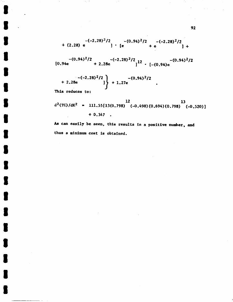
92

-(-2 .2812/2 -(0 -94) 2/2 -(-2.28) 2/2 + e I + + (2.28) e I re

40.94) 2/2 -(-2 . 28) 2/2 12 - (0 .94)2/2 (0.94e + 2.28e 1 [-(0.94)e

-(-2.28) 2/2 40.94) 2/2 + 2.28e This reduces to:

12 13 d2(TC)/dK2 = 111.55[13(0.798) (-0.498) (0.694)(0.798) (-0,520) J

+ 0.347 . As can easily be seen, this results in a positive number, and

thus a minimum cost is obtained.

APPENDIX B

GLOSSABP OF SPWBOLS

1 . 1 - I 8 8 8 I I 8 8 I 1 1 1 I 8 8 I

GLOSSARY OF SYMBOLS

a Probability of rejecting a t rue hypotheses

8 Probabili ty of accepting a f a l s e hypothesis

C Unit cost of the B error

C Unit cost of t h e Q error

C

1

2

3 on the sample s ize . Unit cost of control chart sampling which is d i rec t ly dependent

C Constant defined by a r(n12) r (u-1) /2 2

r Gan~ma function

5 6

e

k

K

oc

Control char t center l i n e

Parameter ref lect ing amount of s h i f t i n some universe parameter

Parameter ref lect ing amount of s h i f t i n some universe parameter i n terms of the standard deviation of the universe parameter

Number of voltage input levels

Input l eve l subscript ( i = 1, 2, ... , h )

Number of subcarrier o sc i l l a to r s

Subcarrier o sc i l l a to r subscript ( j = 1, 2, -.. , m ) Nuder of individual values a t any par t icu lar SCO and input level

Individual value subscript ( k = 1, 2, ... , n )

Control chart l i m i t constant

Operating Characterist ic

94

sco

8’

b i

‘ijk E

P U

‘a

(4 - R

V

UCL

LCL

X2

z

95

Subcarrier o sc i l l a to r

Sample standard deviation

Universe standard deviation

Unbiased estimate of universe standard deviation

Unbiased estimate of standard deviation f o r each input level, i

Average standard deviation

Standard deviation of the d i s t r ibu t ion of standard deviations

Unbiased estimate of the standard deviation among the mean values

A population mean for each input level , i

A universe mean

A sample mean

An average of the sample means

Individual value

Shifted universe mean defined by ? = X’ + &

Shifted universe standard deviation defined by CY;

Precision of the telemetry package

E

6

= a’+ 6

Accuracy of the telemetry package

Variance of the mean values about a theore t ica l curve f i t t e d t o the data

- Average range defined by & - Qn

Degrees of freedom

Upper control chart H m i t

Lower control chart l i m i t

Chi square

Standard normal deviate

8 8

LIST OF REFERENCES

LIST OF REFERENCES

(1) Irving I?. Burr, EnRineerinR Statistics and Quality Control (New York: McGraw-Hill Book Company, Inc., 1953).

(2) Dudley J. Cowden, Statistical Methods in Quality Control (Englewood Cliffs, New Jersey: Prentice-Hall, Inc., 1957) .

Acheson J. Duncan, 'The Economic Design of %-Charts Used to Maintain Current Control of a Process," American Statistical Association Journal, June, 1956, 228-241.

(3)

( 4 ) Acheson J. Duncan, Salitp Control and Industrial Statistics 3rd edition (Homewood, Illinois: Richard D. I n i n , Inc., 1965) .

(5) Marvln A. Griffin and Richard S. Simpson (Project Directors), Accuracy Analysis of F'M/RI Telemetry System far the Saturn Vehicle, Bureau of Engineering Research, University of Alabama, University, Alabama, October, 1963.

(6) Marvin A. Griffin and Richard S. Simpson (Project Directors), Linearity Analysis of the FM/FM Telemetry System, Bureau of Engineering Research, University of Alabama, University, habama,-August, 1965.

(7) Marvin A. Griffin and Richard S. Simpson (Project Directors) , A Statistical Analysis of the Noise and Linearity Charac- teristics of DCS GFD-5, FMR 210, and EMR 67-D Discriminators, Bureau of Engineering Research, University of Alabama, University, Alabama, July, 1965.

( 8 ) Eugene L. Grant, Statistical Quality Control 3rd edition (New York: HcGraw-Hill Book Campany, Inc., 1964).

(9) Paul Go Hoel, Introduction to Mathematical Statistics 3rd edition (New Y a k : John Wiley and Sans, Inc., 1962).

(10) Edgar F. King, "The Operating Characteristic of the Average Chart," Industrial Qual ity Control, November, 1952, 30-32.

97

8 - 8 - I I 1 I 8 8 8 I 8 I 8 8 I 8 I 8

98

(11) Edgar P. King, 'The Operating Characterist ic of the Control Chart f o r Sample Means," Annals of Mathematical S t a t i s t i c s . V o l . 23, 1952, 384-395.

(12) Maurice Sasieni, Arthur Paspan, and Lawrence Friedman, Operation Research-Xe!thods and Problems John W i l q and Sons, Inc., 1959).

(#ew Pork;

(13) W. A. Shewhart, Ecananic Control of Qual i t p of Manufactured Product (Princeton, New Jersey: D. Van Nostrand Cappany, Inc., 1931).

(14) I. S. Sokoln ibf f and R. M. Redheffer, Mathematics of Physics and Modern Engineering (New Pork: NcGraw-Ei l l Book Company, Inc., 1958).

(15) Harry L. S t i l t r (Editor), Aerospace Telemetry (Ensrewood Cl i f f s , New Jersey: Prentice-Hall, Inc., 1963).

BIBLIOGIUPBP

I ' 8 - li 1 8 1 8 I 1 I I I 1 8 1 8 1 I 8

BIBLIOGRAPHY

Books and Reports

Bowker, Albert H, and Lieberman, Gerald J, Engineerinp S t a t i s t i c s . Englewood Cl i f f s , New Jersey: Prentice-Hall, Inc., 1959.

Burr, Irving W. Engineering Statist ics and Qual i ty Control. New York: M c G r a w - H i l l Book Company, Inc., 1953.

Cowden, Dudley J. S t a t i s t i c a l Methods i n Quality Control. E n g l e w d Cliffs , New Jersey: Prentice-Hall, Inc., 1957.

Duncan, Acheson J, Quality Control and Indus t r ia l Statistics. 3rd edit ion. New York: John Wiley and Sons, Inc., 1962.

Goodman, A. w8 Analytic Geometry and the Calculus. New York: The Macmillan Company, 1963.

Grant, Eugene L. S t a t i s t i c a l Quality Control. 3rd edi t ion. New York: McGraw-Hi l l Book Company, Inc., 1964,

Griff in , Marvin A. and Simpson, Richard S. (Project Directors), Accuracy Analysis of FM/FM Telemetry System f o r t he Saturn Vehicle, Bureau of Engineering Research, University of Alabama, University, Alabama, October, 1963.

. Linearity Analysis of the FM/FM Telemetry System, Bureau of Engineering Research, University of Alabama, University, Alabama, August, 1965,

. (Project Directors), A S t a t i s t i c a l Analysis of t he Noise

Bureau of Engineering Research, and Linearity Characterist ics of DCS GFD-5, EMR 210, and EMR 67-D Discriminators, University of Alabama, University, Alabama, July, 1965.

H o e l , Paul G, Introduction to Mathematical S t a t i s t i c s . 3rd edition. New York: John Wiley and Sons, Inc., 1962.

Jurap, J. M. (Editor) Quality Control Handbook. 2nd ed i t ion , New York: M c G r a w - H i l l Book Company, Inc., 1962.

100

I 1 - I I 1 I 1 1 I 5 1 I 1 8 I I I I 1

101

Milne, W i l l i a m Edmund. Numerical Calculus, Princeton, N e v Jersey: Princeton University Press, 1949.

Oven, Donald B. Handbook of S t a t i s t i c a l Tables. Reading, Massachusetts: Addison-Wesley Publishing Company, Inc., 1962.

Sasieni, Maurice, Yaspan, Arthur, and Friedman, Lawrence. Operation Research-Methods and Problems , John Wiley and Sons, Inc. , 1959.

New York:

Shewhart, W. A. Economic Control of Quality of Manufactured Product. Princeton, New Jersey: D. Van Nostrand Company, Inc., 1931.

Sokolnikoff, L. S. and Redheffer, R. M. Hathematics of Physics and Modern Engineerinq. New York: McGraw-Hill Book Company, Inc,, 1958.

S t i l t z , Iiarry L. (Editor) Aerospace Telemetry. Englewwd Cl i f f s , New Jersey: Prentice-Hall, Inc., 1963.

Wiw, -11 R. S t a t i s t i c s f o r Sc ien t i s t s and Engineers. E n g l w d Cliffs , New Jersey: Prentice-Hall, Inc., 1964.

Articles

Craig, C. C. "Control Charts Versus Analysis of Variance in Process Control by Variables," Jan~ary, 1947, 14-16.

Industr ia l Quality Control,

Duncan, Acheson J. "The Economic Design of %Charts Used t o Haintain C u r r e n t Control of a Process," American Statistical Association Journal , June , 1956 , 228-241,

King, Rdgar P. Vhe Operating Characteristic of the Control Chart f o r Sample Means," Annals of Mathematical S ta t i s t ics , Vol. 23, 1932, 384-395.

- . "The Operating Characterist ic of the Average Chart," Idustrial Quality Control, November, 1952, 9-32,

- . "Probability L i m i t s for the Average Chart," Indus t r ia l Quality Control, May, 1954, 10-12.

I . 1 -

Olds, Edvin 6, "Power Characterist ics of Control Charts," Industr ia l Qual i ty Control, July, 1961, 4-9.

102

Scheffe, Henry. "Operating Characteristics of Average and Range Charts," Industr ia l Qual i t9 Cantrol, Hay, 1949, 13-18.

Storm, Leo E. "Specification Study for Limited Production of complex Equipment," Industr ia l Qual i ty Coartrol, February, 1960, 12-18.

Walsh, John E. "Operating Characteristic8 f o r Tests of t he S tab i l i t y of a N o r m a l Population," American S t a t i s t i c a l Association Journal, June, 1952, 191-202.

Weiler, H. "On the Host Economical Sample Size for Controlling the Hean of a Population," Annals of Hathematical S t a t i s - -9 tics Vol. 23, 1952, 247-254.

Documents

REPORT II GROUP 1 - NASA · frequency, a dxer amplifier, a transmitter, and a paver amplifier used for transmitting signals from space vehicle to a ground receiving station. 8 1 -