Research Collection

Master Thesis

Efficiency calculations and optimization analysis of a solarreactor for the high temperature step of the zinc/zinc-oxidethermochemical redox cycle

Author(s): Haussener, Sophia

Publication Date: 2007

Permanent Link: https://doi.org/10.3929/ethz-a-005424125

Rights / License: In Copyright - Non-Commercial Use Permitted

This page was generated automatically upon download from the ETH Zurich Research Collection. For moreinformation please consult the Terms of use.

ETH Library

Master-Thesis

Efficiency calculations and optimization analysis of a solar reactor for the high temperature step of the zinc/zinc-oxide thermochemical redox cycle

Sophia Haussener March 2007

Advisors: Dr. David Hirsch, Dr. Christopher Perkins Prof. Aldo Steinfeld, Prof. Alan Weimer

Institute of Energy Technology Professorship in Renewable Energy Carriers

ETH - Swiss Federal Institute of Technology Zurich

in collaboration with

Department of Chemical and Biological Engineering University of Colorado at Boulder

2

Abstract

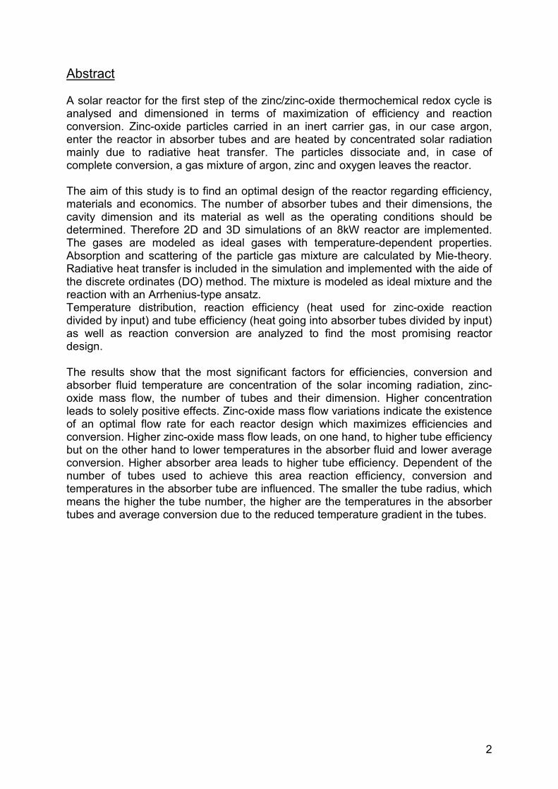
A solar reactor for the first step of the zinc/zinc-oxide thermochemical redox cycle is analysed and dimensioned in terms of maximization of efficiency and reaction conversion. Zinc-oxide particles carried in an inert carrier gas, in our case argon, enter the reactor in absorber tubes and are heated by concentrated solar radiation mainly due to radiative heat transfer. The particles dissociate and, in case of complete conversion, a gas mixture of argon, zinc and oxygen leaves the reactor. The aim of this study is to find an optimal design of the reactor regarding efficiency, materials and economics. The number of absorber tubes and their dimensions, the cavity dimension and its material as well as the operating conditions should be determined. Therefore 2D and 3D simulations of an 8kW reactor are implemented. The gases are modeled as ideal gases with temperature-dependent properties. Absorption and scattering of the particle gas mixture are calculated by Mie-theory. Radiative heat transfer is included in the simulation and implemented with the aide of the discrete ordinates (DO) method. The mixture is modeled as ideal mixture and the reaction with an Arrhenius-type ansatz. Temperature distribution, reaction efficiency (heat used for zinc-oxide reaction divided by input) and tube efficiency (heat going into absorber tubes divided by input) as well as reaction conversion are analyzed to find the most promising reactor design. The results show that the most significant factors for efficiencies, conversion and absorber fluid temperature are concentration of the solar incoming radiation, zinc-oxide mass flow, the number of tubes and their dimension. Higher concentration leads to solely positive effects. Zinc-oxide mass flow variations indicate the existence of an optimal flow rate for each reactor design which maximizes efficiencies and conversion. Higher zinc-oxide mass flow leads, on one hand, to higher tube efficiency but on the other hand to lower temperatures in the absorber fluid and lower average conversion. Higher absorber area leads to higher tube efficiency. Dependent of the number of tubes used to achieve this area reaction efficiency, conversion and temperatures in the absorber tube are influenced. The smaller the tube radius, which means the higher the tube number, the higher are the temperatures in the absorber tubes and average conversion due to the reduced temperature gradient in the tubes.

3

List of Figures

Fig.1-1. Fig.1-2. Fig.1-3. Fig.1-4. Fig.1-5. Fig.1-6. Fig.2-1. Fig.2-2. Fig.2-3. Fig.2-4. Fig.2-5. Fig.2-6. Fig.2-7. Fig.2-8. Fig.2-9. Fig.2-10. Fig.2-11. Fig.2-12. Fig.2-13. Fig.2-14. Fig.2-15. Fig.2-16. Fig.3-1. Fig.3-2.

Fig.3-3. Fig.3-4. Fig.3-5.

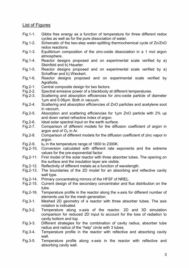
Gibbs free energy as a function of temperature for three different redox cycles as well as for the pure dissociation of water. Schematic of the two-step water-splitting thermochemical cycle of Zn/ZnO redox reactions. Equilibrium composition of the zinc-oxide dissociation in a 1 mol argon atmosphere. Reactor designs proposed and on experimental scale verified by a) Steinfeld and b) Haueter. Reactor designs proposed and on experimental scale verified by a) Schaffner and b) Wieckert. Reactor designs proposed and on experimental scale verified by Agrafiotis. Central composite design for two factors. Spectral emissive power of a blackbody at different temperatures. Scattering and absorption efficiencies for zinc-oxide particle of diameter 1µm and 0.06µm. Both in vacuum. Scattering and absorption efficiencies of ZnO particles and acetylene soot in vaccum. Absorption and scattering efficiencies for 1µm ZnO particle with 2% up and down varied refractive index of argon. Ideal solar spectral input on the earth surface. Comparison of different models for the diffusion coefficient of argon in argon and of O2 in Ar. Comparison of different models for the diffusion coefficient of zinc vapor in argon. k0 in the temperature range of 1800 to 2300K. Conversion calculated with different rate exponents and the extreme values for the pre-exponential factor. First model of the solar reactor with three absorber tubes. The opening on the surface and the insulation layer are visible. Reflectivity of different metals as a function of wavelength. The boundaries of the 2D model for an absorbing and reflective cavity wall type. Primary concentrating mirrors of the HFSF of NREL. Current design of the secondary concentrator and flux distribution on the tube. Temperature profile in the reactor along the x-axis for different number of elements use for the mesh generation. Meshed 2D geometry of a reactor with three absorber tubes. The axis notation is indicated. Temperature along x-axis of the reactor. 2D and 3D simulation comparison for reduced 2D input to account for the loss of radiation to cavity bottom and top. Different strategies for the combination of cavity radius, absorber tube radius and radius of the “help” circle with 3 tubes. Temperature profile in the reactor with reflective and absorbing cavity wall. Temperature profile along x-axis in the reactor with reflective and absorbing cavity wall.

4

Fig.3-6. Fig.3-7. Fig.3-8. Fig.3-9. Fig.3-10.

Fig.3-11. Fig.3-12. Fig.3-13. Fig.3-14. Fig.3-15. Fig.3-16. Fig.4-1. Fig.4-2.

Conversion in the absorber tubes for reflective and absorbing cavity wall. Reflected and absorbed wall flux at the cavity wall for absorbing or reflective cavity wall. Fraction of absorbed and reflected flux (band dependent) on the cavity wall for a reflective and absorbing cavity wall type. Faction of incident radiation in the different bands for the two tubes and two cavity wall types. Pareto charts of the absolute effects of the different factors on tube efficiency, reaction efficiency, average conversion and average absorber tube temperature. Change in absorber fluid temperature to fraction of window area to cavity area. Main effects on tube efficiency for the first and second fractional factorial design. Contour plots for tube efficiency. Contour plots for reaction efficiency. Contour plots for average conversion. Temperature profiles in the rector for different concentrations, different total ZnO mass flow and different tube number and absorber areas. ZnO mass fraction in a reactor with length 0.12m and 0.24m, respectively. Temperature profile in the reactor.

5

List of Tables

Tab.2-1. Tab.2-2. Tab.2-3. Tab.2-4. Tab.2-5.

Tab.2-6. Tab.2-7. Tab.2-8. Tab.3-1. Tab.3-2.

Tab.3-3. Tab.3-4. Tab.3-5. Tab.3-6.

Real and imaginary part of the refractive index used for ZnO particles. Approximated efficiencies for a zinc-oxide particle with 1µm and 0.06µmdiameter in vacuum. Parameters from different references for the diffusion model. The minimal and maximal values of the experimentally investigated values of the constant k0.The minimal and maximal values of the experimentally investigated values of the constant k0 by Perkins [14]. Thermophysical properties of air, argon, oxygen, zinc and zinc-oxide. Thermophysical properties of alumina, quartz and silicon-carbide. Absorption coefficient used for the quartz window in function of the incoming wavelength. Factor definition for the two-level fractional factorial study. Tube and reaction efficiencies, average conversion and average absorber tube temperature for the different simulated cases. Factor definition for the second two-level fractional factorial study. Effects of the different factors on efficiencies, conversion and temperature in absorber fluid. Factor levels (coded and uncoded values) for the CCD design. Definition and results of the full factorial design.

6

Contents

Abstract ………………………………………………………………………………... 2List of Figures …………………………………………………………………………. 3List of Tables ………………………………………………………………………….. 5

1. Introduction ………………………………………………………………………….… 71.1. Thermodynamic analysis ..……….……………………………………………… 71.2. Solar reactor designs ..…….…….……………………………………………….. 91.3. Overview of this project ……………….……………………………………….… 12 2. Models and methods …………………………………………………………….……13 2.1. Mathematical formulation …………………….………………………………….. 13 2.2. Fractional factorial design – Statistics …………..……………………………… 13 2.3. Radiation …………………………………..………………………………………. 16 2.4. Scattering and absorption …….……….………………………………………… 19 2.5. Models for gas diffusion ……………….………………………………………… 23 2.6. Kinetics ……...………………………….…………………………………………. 26 2.7. Thermophysical properties …...….……………….……………………………... 29 2.8. Geometry …………………....……..……………………………………………… 32 2.9. Boundary conditions …………………………………….……………………….. 33 2.10. Grid and conversion study ...………………………………………………..…… 34 2.11. Software ………………………………………………………………………..….. 35 3. Results 2D simulations ….…………………………………………………………… 36 3.1. Difference between 2D and 3D simulations …………………………………….. 36 3.2. Simulation parameters ………………..…………………………………………… 37 3.3. Fractional factorial designs ………………………………..……………………... 39 3.4. Response surface design – Central composite design study ………………... 45 3.5 Full factorial design …………..……………………………..……………………... 48 4. Results 3D simulations ……………………………………...………………………..50 5. Conclusions and suggestions for future work ……………..……………………….51 6. Acknowledgements …………………………………………………………………...52 7. References ……………………………………………………………………………. 53

Appendix A ....………………………………………………………………………….Appendix B …………………………………………………………………………….Appendix C …………………………………………………………………………….Appendix D …………………………………………………………………………….Appendix E …………………………………………………………………………….Appendix F …………………………………………………………………………….Appendix G …………………………………………………………………………….Appendix H …………………………………………………………………………….Appendix I …………………………………………………………………………….

56 57 59 60 64 67 68 69 70

7

1. Introduction

To overcome the problem of shortening reserves of the three major (and non-renewable) energy carriers coal, oil and natural gas as well as the environmental pollution caused by them and their main impact on the manmade [1] increased carbon dioxide concentration in the atmosphere, new and clean ways of energy conversion should be investigated. This task lies on the challenging background of further increase in global energy consumption [2]. Clearly the priority needs to lie on renewable and non pollutant emitting energy conversion concepts, which use sun, wind, water (including hydropower and ocean resources), geothermal heat and biomass. Due to the transient nature of some renewable energy sources energy storage is critical. The focus of this work lies on solar energy. There are several ways to convert solar energy to useful energy. Photovoltaics convert the energy of a photon directly to electrical energy. So far this solution suffers from relatively poor efficiencies (around 15%) and high production costs. Unconcentrated solar light is used for several low temperature applications like heating of water and air. To achieve higher temperatures diluted solar light is concentrated by large parabolic reflector systems (trough, tower, dish [3]). Temperatures up to 2100K can be achieved and are used to run several chemical cycles in a sustainable way. Waste treatment [4], capturing of atmospheric carbon dioxide [5], gasification of coal or petroleum coke [6-8], methane dissociation and reforming [9-11], lime production [12] and several metal/metal-oxide cycles [13] are some examples. As additional or main target, hydrogen is produced with these processes. By using solar high-temperature heat, this hydrogen stores the solar energy. Some of the advantages of hydrogen as energy carrier are relatively high specific energy density and efficient direct conversion to other forms of energy (not limited by the Carnot efficiency). So far the main portion of the globally produced hydrogen is fabricated by decarbonisation of fossil energy carriers. This is a non-renewable way and should be prevented in the near future. Electrolysis of water suffers from low efficiencies and can only be assumed sustainable when the used electricity is produced by renewable energy sources. Therefore using solar high-temperature heat to produce hydrogen is a new and promising solution for a clean way to produce hydrogen. Direct water splitting and metal/metal-oxide cycles are two high temperature ways to produce hydrogen without the need of carbonaceous sources. Direct splitting of water takes place at very high temperatures due to unfavorable thermodynamics and there is still not an efficient way to separate the products. Therefore metal/metal-oxide cycles are more promising. They lower the needed temperature and, with at least two separate steps of the cycle, there is no additional need for high-temperature gas separation and no formation of explosive mixtures.

1.1. Thermodynamic analysis

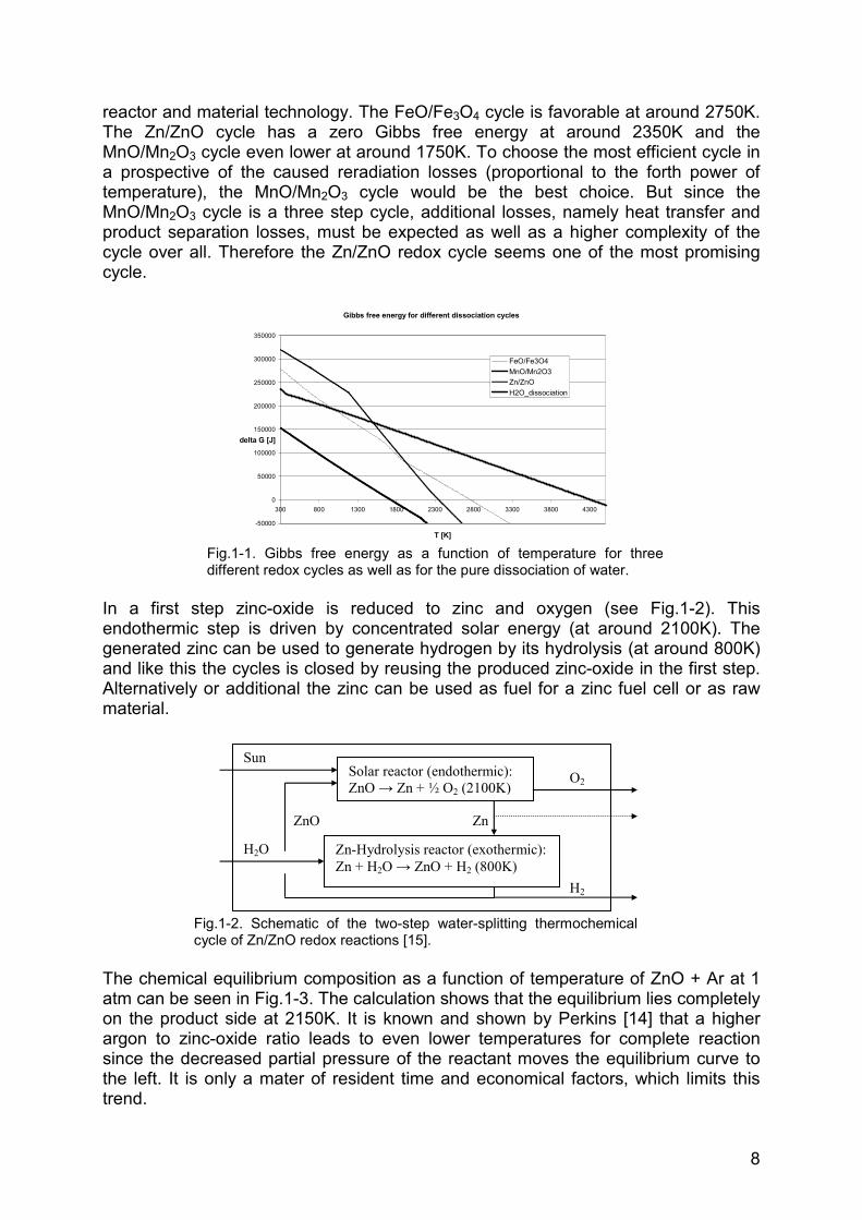
Several metal/metal-oxide cycles have been thermodynamically analyzed by Perkins [14]. The analysis of three of the most popular and promising metal-metaloxide cycles have been reproduced: Zn/ZnO, FeO/Fe3O4 and MnO/Mn2O3. Fig.1-1 shows the calculated free Gibbs energy of these three metal/metal-oxide cycles and of direct water dissociation. These calculations were performed with FACT software. The dissociation temperature of direct water dissociation turns out to be around 4300K. This temperature is not easy if not impossible to reach and withstand with known

8

reactor and material technology. The FeO/Fe3O4 cycle is favorable at around 2750K. The Zn/ZnO cycle has a zero Gibbs free energy at around 2350K and the MnO/Mn2O3 cycle even lower at around 1750K. To choose the most efficient cycle in a prospective of the caused reradiation losses (proportional to the forth power of temperature), the MnO/Mn2O3 cycle would be the best choice. But since the MnO/Mn2O3 cycle is a three step cycle, additional losses, namely heat transfer and product separation losses, must be expected as well as a higher complexity of the cycle over all. Therefore the Zn/ZnO redox cycle seems one of the most promising cycle.

Gibbs free energy for different dissociation cycles

-50000

0

50000

100000

150000

200000

250000

300000

350000

300 800 1300 1800 2300 2800 3300 3800 4300

T [K]

delta G [J]

FeO/Fe3O4MnO/Mn2O3Zn/ZnOH2O_dissociation

Fig.1-1. Gibbs free energy as a function of temperature for three different redox cycles as well as for the pure dissociation of water.

In a first step zinc-oxide is reduced to zinc and oxygen (see Fig.1-2). This endothermic step is driven by concentrated solar energy (at around 2100K). The generated zinc can be used to generate hydrogen by its hydrolysis (at around 800K) and like this the cycles is closed by reusing the produced zinc-oxide in the first step. Alternatively or additional the zinc can be used as fuel for a zinc fuel cell or as raw material.

Fig.1-2. Schematic of the two-step water-splitting thermochemical cycle of Zn/ZnO redox reactions [15].

The chemical equilibrium composition as a function of temperature of ZnO + Ar at 1 atm can be seen in Fig.1-3. The calculation shows that the equilibrium lies completely on the product side at 2150K. It is known and shown by Perkins [14] that a higher argon to zinc-oxide ratio leads to even lower temperatures for complete reaction since the decreased partial pressure of the reactant moves the equilibrium curve to the left. It is only a mater of resident time and economical factors, which limits this trend.

Solar reactor (endothermic): ZnO → Zn + ½ O2 (2100K)

O2

Zn-Hydrolysis reactor (exothermic): Zn + H2O→ ZnO + H2 (800K)

H2

Zn

ZnO

H2O

Sun

9

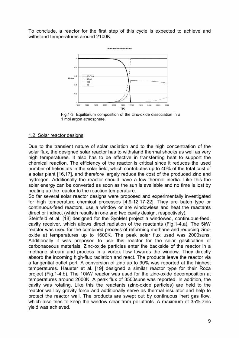
To conclude, a reactor for the first step of this cycle is expected to achieve and withstand temperatures around 2100K.

Equilibrium composition

0

0.2

0.4

0.6

0.8

1

1000 1200 1400 1600 1800 2000 2200 2400 2600 2800 3000

T [K]

MolesZnO(s)Zn(g)O2O

Fig.1-3. Equilibrium composition of the zinc-oxide dissociation in a 1 mol argon atmosphere.

1.2. Solar reactor designs

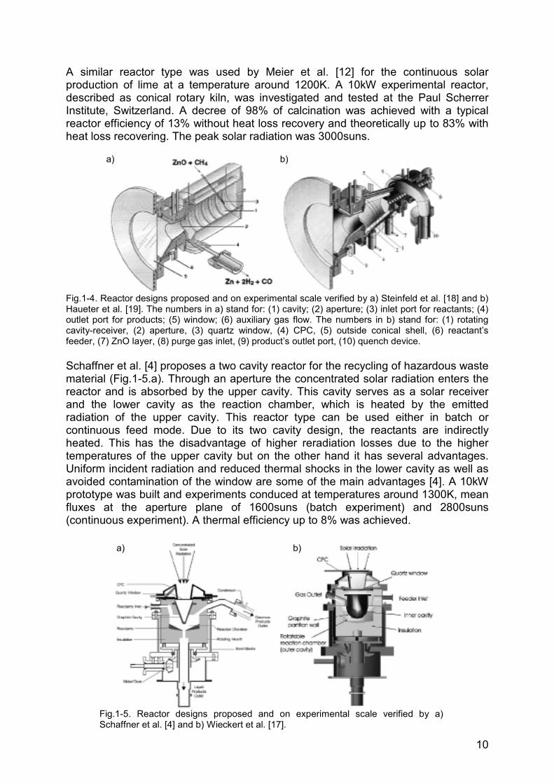
Due to the transient nature of solar radiation and to the high concentration of the solar flux, the designed solar reactor has to withstand thermal shocks as well as very high temperatures. It also has to be effective in transferring heat to support the chemical reaction. The efficiency of the reactor is critical since it reduces the used number of heliostats in the solar field, which contributes up to 40% of the total cost of a solar plant [16,17], and therefore largely reduce the cost of the produced zinc and hydrogen. Additionally the reactor should have a low thermal inertia. Like this the solar energy can be converted as soon as the sun is available and no time is lost by heating up the reactor to the reaction temperature. So far several solar reactor designs were proposed and experimentally investigated for high temperature chemical processes [4,9-12,17-22]. They are batch type or continuous-feed reactors, use a window or are windowless and heat the reactants direct or indirect (which results in one and two cavity design, respectively). Steinfeld et al. [18] designed for the SynMet project a windowed, continuous-feed, cavity receiver, which allows direct radiation of the reactants (Fig.1-4.a). The 5kW reactor was used for the combined process of reforming methane and reducing zinc-oxide at temperatures up to 1600K. The peak solar flux used was 2000suns. Additionally it was proposed to use this reactor for the solar gasification of carbonaceous materials. Zinc-oxide particles enter the backside of the reactor in a methane stream and process in a vortex flow towards the window. They directly absorb the incoming high-flux radiation and react. The products leave the reactor via a tangential outlet port. A conversion of zinc up to 90% was reported at the highest temperatures. Haueter et al. [19] designed a similar reactor type for their Roca project (Fig.1-4.b). The 10kW reactor was used for the zinc-oxide decomposition at temperatures around 2000K. A peak flux of 3500suns was reported. In addition, the cavity was rotating. Like this the reactants (zinc-oxide particles) are held to the reactor wall by gravity force and additionally serve as thermal insulator and help to protect the reactor wall. The products are swept out by continuous inert gas flow, which also tries to keep the window clear from pollutants. A maximum of 35% zinc yield was achieved.

10

A similar reactor type was used by Meier et al. [12] for the continuous solar production of lime at a temperature around 1200K. A 10kW experimental reactor, described as conical rotary kiln, was investigated and tested at the Paul Scherrer Institute, Switzerland. A decree of 98% of calcination was achieved with a typical reactor efficiency of 13% without heat loss recovery and theoretically up to 83% with heat loss recovering. The peak solar radiation was 3000suns.

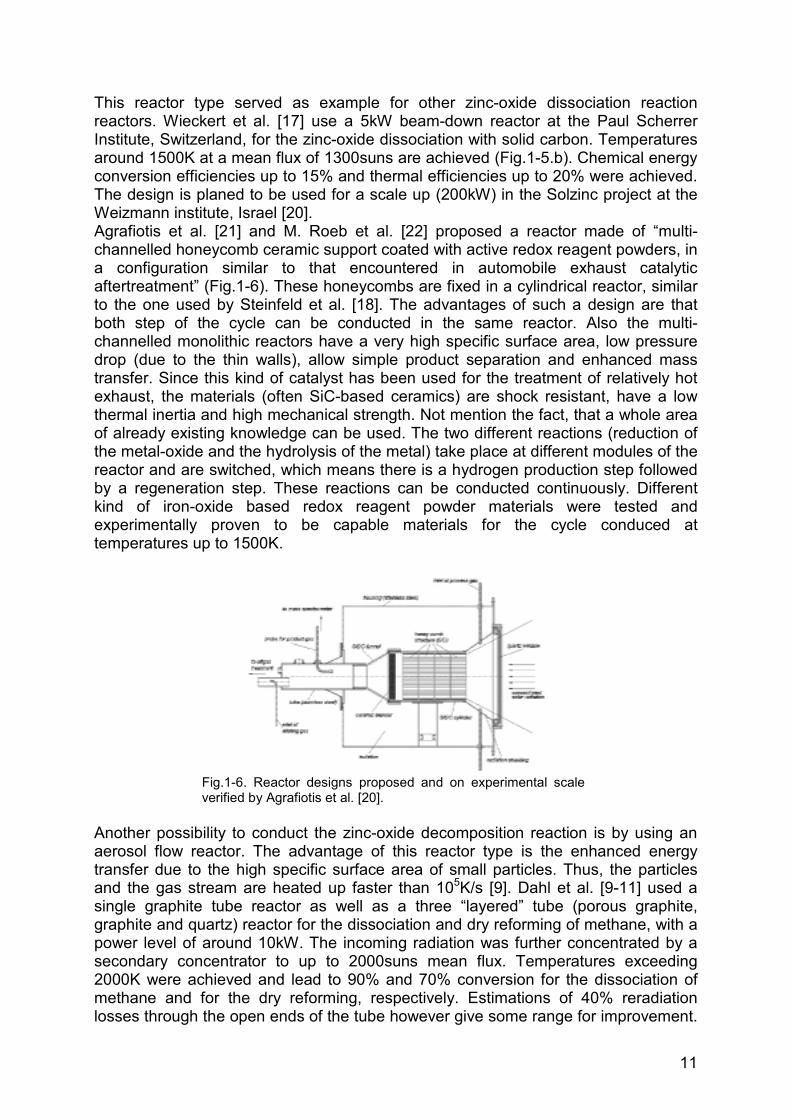
Fig.1-4. Reactor designs proposed and on experimental scale verified by a) Steinfeld et al. [18] and b) Haueter et al. [19]. The numbers in a) stand for: (1) cavity; (2) aperture; (3) inlet port for reactants; (4) outlet port for products; (5) window; (6) auxiliary gas flow. The numbers in b) stand for: (1) rotating cavity-receiver, (2) aperture, (3) quartz window, (4) CPC, (5) outside conical shell, (6) reactant’s feeder, (7) ZnO layer, (8) purge gas inlet, (9) product’s outlet port, (10) quench device. Schaffner et al. [4] proposes a two cavity reactor for the recycling of hazardous waste material (Fig.1-5.a). Through an aperture the concentrated solar radiation enters the reactor and is absorbed by the upper cavity. This cavity serves as a solar receiver and the lower cavity as the reaction chamber, which is heated by the emitted radiation of the upper cavity. This reactor type can be used either in batch or continuous feed mode. Due to its two cavity design, the reactants are indirectly heated. This has the disadvantage of higher reradiation losses due to the higher temperatures of the upper cavity but on the other hand it has several advantages. Uniform incident radiation and reduced thermal shocks in the lower cavity as well as avoided contamination of the window are some of the main advantages [4]. A 10kW prototype was built and experiments conduced at temperatures around 1300K, mean fluxes at the aperture plane of 1600suns (batch experiment) and 2800suns (continuous experiment). A thermal efficiency up to 8% was achieved.

Fig.1-5. Reactor designs proposed and on experimental scale verified by a) Schaffner et al. [4] and b) Wieckert et al. [17].

a) b)

a) b)

11

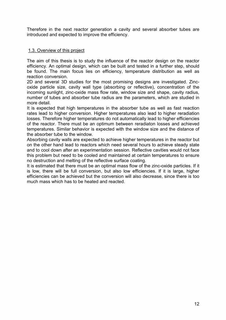
This reactor type served as example for other zinc-oxide dissociation reaction reactors. Wieckert et al. [17] use a 5kW beam-down reactor at the Paul Scherrer Institute, Switzerland, for the zinc-oxide dissociation with solid carbon. Temperatures around 1500K at a mean flux of 1300suns are achieved (Fig.1-5.b). Chemical energy conversion efficiencies up to 15% and thermal efficiencies up to 20% were achieved. The design is planed to be used for a scale up (200kW) in the Solzinc project at the Weizmann institute, Israel [20]. Agrafiotis et al. [21] and M. Roeb et al. [22] proposed a reactor made of “multi-channelled honeycomb ceramic support coated with active redox reagent powders, in a configuration similar to that encountered in automobile exhaust catalytic aftertreatment” (Fig.1-6). These honeycombs are fixed in a cylindrical reactor, similar to the one used by Steinfeld et al. [18]. The advantages of such a design are that both step of the cycle can be conducted in the same reactor. Also the multi-channelled monolithic reactors have a very high specific surface area, low pressure drop (due to the thin walls), allow simple product separation and enhanced mass transfer. Since this kind of catalyst has been used for the treatment of relatively hot exhaust, the materials (often SiC-based ceramics) are shock resistant, have a low thermal inertia and high mechanical strength. Not mention the fact, that a whole area of already existing knowledge can be used. The two different reactions (reduction of the metal-oxide and the hydrolysis of the metal) take place at different modules of the reactor and are switched, which means there is a hydrogen production step followed by a regeneration step. These reactions can be conducted continuously. Different kind of iron-oxide based redox reagent powder materials were tested and experimentally proven to be capable materials for the cycle conduced at temperatures up to 1500K.

Fig.1-6. Reactor designs proposed and on experimental scale verified by Agrafiotis et al. [20].

Another possibility to conduct the zinc-oxide decomposition reaction is by using an aerosol flow reactor. The advantage of this reactor type is the enhanced energy transfer due to the high specific surface area of small particles. Thus, the particles and the gas stream are heated up faster than 105K/s [9]. Dahl et al. [9-11] used a single graphite tube reactor as well as a three “layered” tube (porous graphite, graphite and quartz) reactor for the dissociation and dry reforming of methane, with a power level of around 10kW. The incoming radiation was further concentrated by a secondary concentrator to up to 2000suns mean flux. Temperatures exceeding 2000K were achieved and lead to 90% and 70% conversion for the dissociation of methane and for the dry reforming, respectively. Estimations of 40% reradiation losses through the open ends of the tube however give some range for improvement.

12

Therefore in the next reactor generation a cavity and several absorber tubes are introduced and expected to improve the efficiency.

1.3. Overview of this project

The aim of this thesis is to study the influence of the reactor design on the reactor efficiency. An optimal design, which can be built and tested in a further step, should be found. The main focus lies on efficiency, temperature distribution as well as reaction conversion. 2D and several 3D studies for the most promising designs are investigated. Zinc-oxide particle size, cavity wall type (absorbing or reflective), concentration of the incoming sunlight, zinc-oxide mass flow rate, window size and shape, cavity radius, number of tubes and absorber tube radius are the parameters, which are studied in more detail. It is expected that high temperatures in the absorber tube as well as fast reaction rates lead to higher conversion. Higher temperatures also lead to higher reradiation losses. Therefore higher temperatures do not automatically lead to higher efficiencies of the reactor. There must be an optimum between reradiaton losses and achieved temperatures. Similar behavior is expected with the window size and the distance of the absorber tube to the window. Absorbing cavity walls are expected to achieve higher temperatures in the reactor but on the other hand lead to reactors which need several hours to achieve steady state and to cool down after an experimentation session. Reflective cavities would not face this problem but need to be cooled and maintained at certain temperatures to ensure no destruction and melting of the reflective surface coating. It is estimated that there must be an optimal mass flow of the zinc-oxide particles. If it is low, there will be full conversion, but also low efficiencies. If it is large, higher efficiencies can be achieved but the conversion will also decrease, since there is too much mass which has to be heated and reacted.

13

2. Models and methods

The design parameters for the simulation studies are introduced in this chapter. The mathematical model and the statistical method used to reduce the simulation number are presented. Theoretical insight in radiation heat transfer and Mie-theory are given in the next subchapters. Modes for gas diffusivity and kinetic parameters are studied and presented. The geometry and the boundary conditions are discussed in the following subchapters. Finally grid and conversion studies are presented and a short description of the used commercial CFD code is given.

2.1. Mathematical formulation

The covering equations for the studied problem are the continuity equation (2.1), momentum equations (2.2) and scalar equations for energy and for the concentration of every fraction of the mixture (2.3).

0)( =⋅∂∂+

∂∂

jj

uxt

ρρ (2.1)

∂

∂+

∂∂

∂∂+

∂∂

−=⋅⋅∂∂+⋅

∂∂

i

j

j

i

jiij

ji x

uxu

xxpuu

xu

tµρρ )()( (2.2)

Φ+

∂Φ∂

Γ∂∂=Φ⋅⋅

∂∂+Φ⋅

∂∂ S

xxu

xt jjj

j

)()( ρρ (2.3)

ρ denotes the density, u the velocity vector, p the pressure, µ the dynamic viscosity, Φ the scalar (enthalpy or concentration), Γ variable for the properties of the media (thermal conductivity, heat capacity or diffusion coefficient) and SΦ the source term. For the energy equation this source term will include the flux which is generated due to radiative heat transfer.

2.2. Fractional factorial design – Statistics

To study the influence of different parameters on a specific property of interest in a specific design, different methods can be investigated. Either there is the best guess approach. An experiment or simulation is investigated and due to the result different parameters are adapted and like this an optimum is tried to be achieved. This approach needs a lot of technical and theoretical knowledge for a problem. But often exactly this knowledge is tried to be achieved with the aid of experiments. A more accurate and structured approach is the “one-factor-at-a-time” approach. Several experiments or simulations are investigated. Starting from a reference case, only a parameter at a time is changed and the other parameters are held constant. Although this approach can give good insight into the problem, it does not investigate the effect of interaction between different parameters. To overcome this problem there exist the factorial design approach. In this analysis, all possible combination of parameters are investigated and analyzed. As the number of interaction varies exponentially

14

(kn=levelsfactors) already a moderate number of factors requires a very large number of experiments. Therefore the so called fractional factorial design can be investigated. It reduces the number of used experiments or simulation by assuming that higher order interactions can be neglected. There exists several so called resolution of a fractional factional factorial design, dependent on how many higher order interactions are neglected or aliased with lower order interactions. Statistics is used to allow conclusions even if not all possible combinations are investigated. Since we will investigate 8 different factors (n) with two levels (k) of the effects, maximal 28=256 possible combinations must be analyzed. A resolution IV design will reduce the number of used experiments to 28-4 or 28-3 by aliasing three order interactions with main effects and two order interactions with each other. The disadvantage of such a resolution is, that no clear statements can be made for the second order interactions, since these are aliased with each other (see appendix A1 for the alias structure). On the other hand the number of experiments is just a small fraction of the initial 256 combinations. A resolution V design reduces the number of used experiments to 28-2 combinations. The larger number is purchased by more information about the second order interactions, since they are now only aliased with third order interactions. The results are statistically analyzed (Minitab 14.1 software was used). A good introduction into statistical data processing of fractional design is given by Montgomery [23]. The method for analyzing the data is the so called Analysis of Variance (ANOVA) method. For simplicity the method is presented for a single factor. Additional “dimensions” must be added to include more than one factor [23]. The ANOVA analysis compares the data to the so called effect model (2.4).

==

++=njai

y ijiij ,...2,1,...2,1

ετµ (2.4)

yij is the ijth observation, µ the overall mean, τi the ith treatment effect and εij the random error (important for experiments, to account for variation between different runs with the same conditions). i is the number of treatment and j is the number of observation at a specific treatment level. (2.4) is a linear statistical model. This should be in mind when analyzing the data. Two assumptions have to be valid for the ANOVA method to be useable. First the residuals have to be normally distributed and second the residuals have to be uncorrelated. The hypothesis (2.5) is tested to make statistical conclusions about the significance of effects on a specific output behavior.

H0: τ1= τ 2=…= τ a=0 H1: τ i≠0 for at least one i

It can be shown [23] that the appropriate test statistic for the fraction of the normalized sum of square due to treatments (2.6) and the normalized sum of square due to error (2.7) is the F-distribution with a-1 and N-a degrees of freedom (N=an).

1

)(

11

2...

−

−=

−

∑=

a

yyn

aSS

a

ii

Treatments (2.6)

aN

yy

aNSS

a

i

n

jiij

E

−

−=

−

∑∑= =1 1

2.)(

(2.7)

(2.5)

15

yij is the ijth observation, .iy is the average of the observation under the ith treatment (2.8) and ..y represents the grand average of all the observations (2.9).

∑=

==n

jij

ii y

nnyy

1

..

1 (2.8)

∑∑= =

==a

i

n

jijy

NNyy

1 1

....

1 (2.9)

The F-distribution is defined as follows:

vuF

v

uvu /

/2

2

, χχ= (2.10)

2uχ and 2

vχ are chi-square distributed variables with freedom u and v, respectively. The density function of the chi-square distribution with k degrees of freedom is defined as follows:

2/1)2/(2/ )2/(2

1)( xkk ex

kxf −−

Γ= (2.11)

Γ is the gamma function (2.12). The density distribution of the F-distribution is defined as (2.13).

dtetx tx∫∞

−−=Γ0

1)( (2.12)

2/)(

1)2/(2/

12

2)( vu

uu

xvuv

xu

xvuvu

xh +

−

+

Γ

Γ

+

Γ= (2.13)

When testing the hypothesis, two kinds of errors may be committed. If the null hypothesis (H0) is rejected when it is true, a type I error has occurred. If the null hypothesis is not rejected when it is false, a type II error has been made. The general procedure in hypothesis testing is to specify a value of the probability of type I error and then design the test procedure so that the probability of type II error is suitably small. Values for the F-distribution at different confidence interval (confidence interval is defined as 100% - type I error probability) can be found in literature [23]. Hypothesis testing will give us ideas about the significance of several factors on the system behavior. To gain more and detailed insight in the behavior, a response surface design is investigated next in the most promising region. A common used second order design is the central composite design (CCD). With the aide of a specific design fewer runs are needed to estimate a second order fit (2.14). The least squares method is used to estimate the parameters (β) in the approximating

16

polynomial. CCD leads to empirical models and allows obtaining a more precise estimate of the optimum operating conditions of the process.

∑ ∑∑∑ <==

++++=ji jiij

k

iiii

k

iii xxxxy εββββ

1

2

10 (2.14)

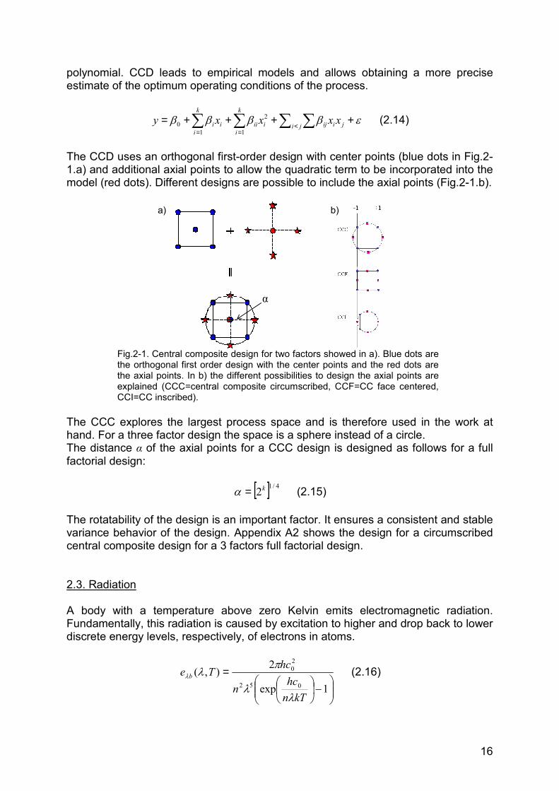
The CCD uses an orthogonal first-order design with center points (blue dots in Fig.2-1.a) and additional axial points to allow the quadratic term to be incorporated into the model (red dots). Different designs are possible to include the axial points (Fig.2-1.b).

Fig.2-1. Central composite design for two factors showed in a). Blue dots are the orthogonal first order design with the center points and the red dots are the axial points. In b) the different possibilities to design the axial points are explained (CCC=central composite circumscribed, CCF=CC face centered, CCI=CC inscribed).

The CCC explores the largest process space and is therefore used in the work at hand. For a three factor design the space is a sphere instead of a circle. The distance α of the axial points for a CCC design is designed as follows for a full factorial design:

[ ] 4/12k=α (2.15) The rotatability of the design is an important factor. It ensures a consistent and stable variance behavior of the design. Appendix A2 shows the design for a circumscribed central composite design for a 3 factors full factorial design.

2.3. Radiation

A body with a temperature above zero Kelvin emits electromagnetic radiation. Fundamentally, this radiation is caused by excitation to higher and drop back to lower discrete energy levels, respectively, of electrons in atoms.

−

=1exp

2),(

052

20

kTnhcn

hcTe b

λλ

πλλ (2.16)

a) b)

α

17

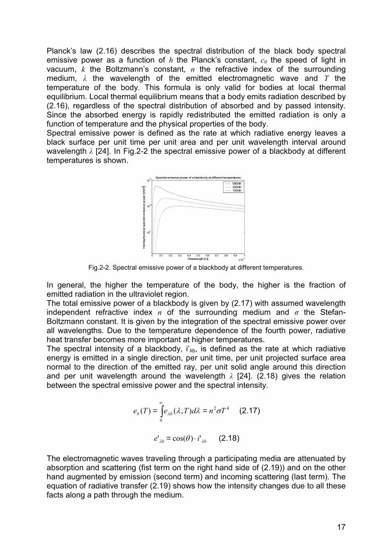
Planck’s law (2.16) describes the spectral distribution of the black body spectral emissive power as a function of h the Planck’s constant, c0 the speed of light in vacuum, k the Boltzmann’s constant, n the refractive index of the surrounding medium, λ the wavelength of the emitted electromagnetic wave and T the temperature of the body. This formula is only valid for bodies at local thermal equilibrium. Local thermal equilibrium means that a body emits radiation described by (2.16), regardless of the spectral distribution of absorbed and by passed intensity. Since the absorbed energy is rapidly redistributed the emitted radiation is only a function of temperature and the physical properties of the body. Spectral emissive power is defined as the rate at which radiative energy leaves a black surface per unit time per unit area and per unit wavelength interval around wavelength λ [24]. In Fig.2-2 the spectral emissive power of a blackbody at different temperatures is shown.

0 0.1 0.2 0.3 0.4 0.5 0.6 0.7 0.8 0.9 1

x10-5

105

1010

1015 Spectral emissive power of a blackbody at different temperatures

Wavelength [m]

Hem

isph

ceric

alsp

ectra

lem

issi

vepo

wer

[W/m

3 ]

5800K2000K1000K

Fig.2-2. Spectral emissive power of a blackbody at different temperatures. In general, the higher the temperature of the body, the higher is the fraction of emitted radiation in the ultraviolet region. The total emissive power of a blackbody is given by (2.17) with assumed wavelength independent refractive index n of the surrounding medium and σ the Stefan-Boltzmann constant. It is given by the integration of the spectral emissive power over all wavelengths. Due to the temperature dependence of the fourth power, radiative heat transfer becomes more important at higher temperatures. The spectral intensity of a blackbody, i’λb, is defined as the rate at which radiative energy is emitted in a single direction, per unit time, per unit projected surface area normal to the direction of the emitted ray, per unit solid angle around this direction and per unit wavelength around the wavelength λ [24]. (2.18) gives the relation between the spectral emissive power and the spectral intensity.

42

0

),()( TndTeTe bb σλλλ == ∫∞

(2.17)

bb ie λλ θ ')cos(' ⋅= (2.18)

The electromagnetic waves traveling through a participating media are attenuated by absorption and scattering (fist term on the right hand side of (2.19)) and on the other hand augmented by emission (second term) and incoming scattering (last term). The equation of radiative transfer (2.19) shows how the intensity changes due to all these facts along a path through the medium.

18

∫ Φ+⋅+⋅−=i

iiis

b dsisiasids

di

ωλλ

λλλλλ

λ ωωωλωπ

σκ ),,(),('

4)(')('

' (2.19)

κλ is the extinction coefficient, defined by (2.20). aλ is the absorption coefficient, σλ the scattering coefficient and Φ the scattering phase function defined by (2.21).

λλλ σκ += a (2.20)

∫=Φ

i

is

s

ddi

di

ωλ

λλ

ωϕθπ

ϕθϕθ

),('41

),('),(

,

, (2.21)

The energy equation (2.22) includes the effect of radiation by the divergence of the radiative heat flux, which can be calculated with the aid of the built divergence of the intensity (2.23).

drp qqTkDtDPT

DtDTc Φ++−∇⋅∇+= ''')(βρ (2.22)

ωπ

dsiqr ∫ ⋅⋅=4

0

' (2.23)

It is also possible to calculate the divergence of the radiant heat flux vector directly. This yields to (2.24).

∫ ∫∞

−⋅=∇0

4

0

])(''4[ λωωππ

λλλ ddiiaq br (2.24)

(2.24) is derived by using the relation (2.25) and integrating it over all λ, which is nothing else but integrating the equation of radiative transfer over all directions and wavelengths.

λλλλ

ω

λ ω rzryrxrb q

zq

yq

xq

dds

di∇=

∂∂

+∂

∂+

∂∂

=∫ ,,,' (2.25)

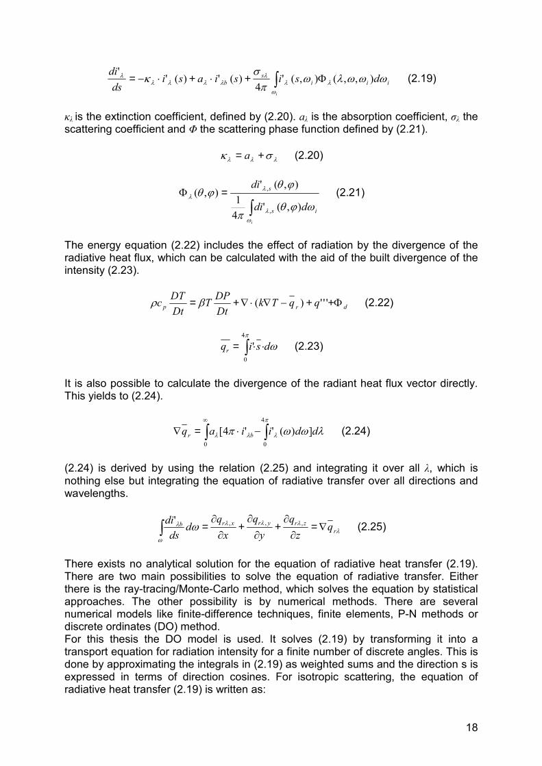
There exists no analytical solution for the equation of radiative heat transfer (2.19). There are two main possibilities to solve the equation of radiative transfer. Either there is the ray-tracing/Monte-Carlo method, which solves the equation by statistical approaches. The other possibility is by numerical methods. There are several numerical models like finite-difference techniques, finite elements, P-N methods or discrete ordinates (DO) method. For this thesis the DO model is used. It solves (2.19) by transforming it into a transport equation for radiation intensity for a finite number of discrete angles. This is done by approximating the integrals in (2.19) as weighted sums and the direction s is expressed in terms of direction cosines. For isotropic scattering, the equation of radiative heat transfer (2.19) is written as:

19

∑∑ Ω+Ω−=+

∂∂

=''

3

1

'4

')1(''mmbm

mi ii iwiiil

πκ(2.26)

where w is a weighting factor, m and m’ denotes ordinate directions, li is the direction cosine of the m direction relative to the coordinate direction i, Ω is the Albedo, defined by (2.27) and κ is the optical thickness.

a+=Ωσσ (2.27)

The number of ordinates has to be defined and set in a way that calculation expense and accuracy are in a healthy balance. Each octant of the angular space 4ω at any spatial location is discretized in number of Nθ and Nφ solid angles. θ is the polar and φthe azimuthal angle. For a 3D simulation 8·Nθ·Nφ equations have to be solved, while for a 2D simulation only 4·Nθ·Nφ have to be calculated. Following recommendations [25] Nθ and Nφ are set to 4 in the work at hand. Studies verified this assumption, increasing the numbers of angles to 5 yields a maximal temperature difference of 10 degrees. This is (compared to an average temperature of around 2000K) less than 0.5% while the simulation time would be 1.56 times higher.

2.4. Scattering and absorption

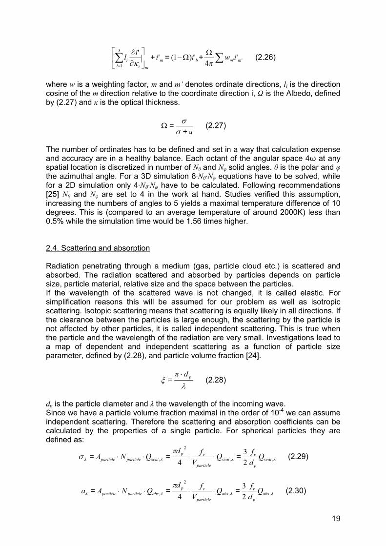
Radiation penetrating through a medium (gas, particle cloud etc.) is scattered and absorbed. The radiation scattered and absorbed by particles depends on particle size, particle material, relative size and the space between the particles. If the wavelength of the scattered wave is not changed, it is called elastic. For simplification reasons this will be assumed for our problem as well as isotropic scattering. Isotopic scattering means that scattering is equally likely in all directions. If the clearance between the particles is large enough, the scattering by the particle is not affected by other particles, it is called independent scattering. This is true when the particle and the wavelength of the radiation are very small. Investigations lead to a map of dependent and independent scattering as a function of particle size parameter, defined by (2.28), and particle volume fraction [24].

λπ

ξ pd⋅= (2.28)

dp is the particle diameter and λ the wavelength of the incoming wave. Since we have a particle volume fraction maximal in the order of 10-4 we can assume independent scattering. Therefore the scattering and absorption coefficients can be calculated by the properties of a single particle. For spherical particles they are defined as:

λλλλ

πσ ,,

2

, 23

4 scatp

vscat

particle

vpscatparticleparticle Q

dfQ

Vfd

QNA =⋅⋅=⋅⋅= (2.29)

λλλλ

π,,

2

, 23

4 absp

vabs

particle

vpabsparticleparticle Q

dfQ

Vfd

QNAa =⋅⋅=⋅⋅= (2.30)

20

with the scattering coefficient σλ, absorption coefficient aλ, Aparticle the geometric article cross section, Nparticle the particle number, fv the volume fraction, Vparticle the volume of a single particle, dp the particle diameter, Qscat,λ the scattering efficiency and Qabs,λ the absorption efficiency. The efficiencies are defined as ratio of scattering and absorption cross section, respectively, to the geometrical cross section:

particle

scatscat A

CQ λ

λ,

, = (2.31)

particle

absabs A

CQ λ

λ,

, = (2.32)

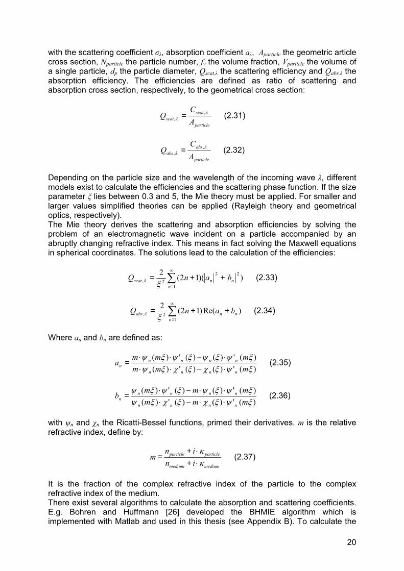
Depending on the particle size and the wavelength of the incoming wave λ, different models exist to calculate the efficiencies and the scattering phase function. If the size parameter ξ lies between 0.3 and 5, the Mie theory must be applied. For smaller and larger values simplified theories can be applied (Rayleigh theory and geometrical optics, respectively). The Mie theory derives the scattering and absorption efficiencies by solving the problem of an electromagnetic wave incident on a particle accompanied by an abruptly changing refractive index. This means in fact solving the Maxwell equations in spherical coordinates. The solutions lead to the calculation of the efficiencies:

∑∞

=

++=1

22

2, ))(12(2n

nnscat banQξλ (2.33)

∑∞

=

++=1

2, )Re()12(2n

nnabs banQξλ (2.34)

Where an and bn are defined as:

)(')()(')()(')()(')(

ξψξχξχξψξψξψξψξψ

mmmmmm

annnn

nnnnn ⋅−⋅⋅

⋅−⋅⋅= (2.35)

)(')()(')()(')()(')(

ξψξχξχξψξψξψξψξψ

mmmmmm

bnnnn

nnnnn ⋅⋅−⋅

⋅⋅−⋅= (2.36)

with ψn and χn the Ricatti-Bessel functions, primed their derivatives. m is the relative refractive index, define by:

mediummedium

particleparticle

inin

mκκ⋅+⋅+

= (2.37)

It is the fraction of the complex refractive index of the particle to the complex refractive index of the medium. There exist several algorithms to calculate the absorption and scattering coefficients. E.g. Bohren and Huffmann [26] developed the BHMIE algorithm which is implemented with Matlab and used in this thesis (see Appendix B). To calculate the

21

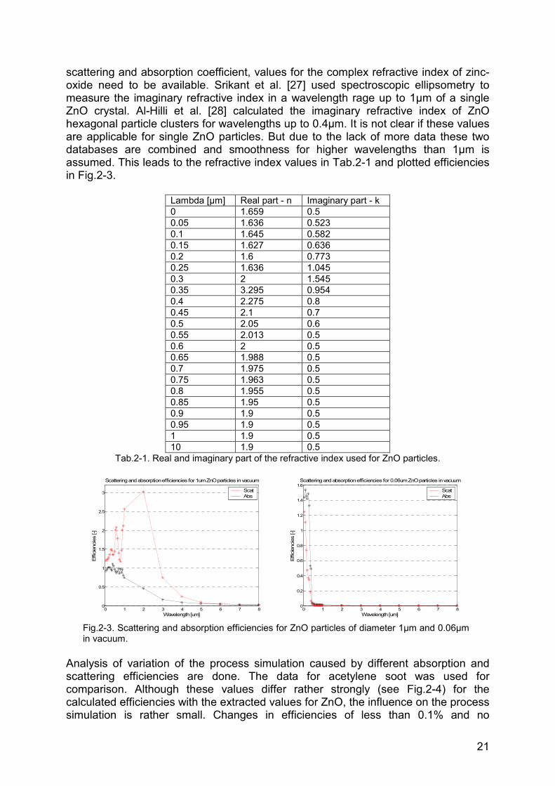
scattering and absorption coefficient, values for the complex refractive index of zinc-oxide need to be available. Srikant et al. [27] used spectroscopic ellipsometry to measure the imaginary refractive index in a wavelength rage up to 1µm of a single ZnO crystal. Al-Hilli et al. [28] calculated the imaginary refractive index of ZnO hexagonal particle clusters for wavelengths up to 0.4µm. It is not clear if these values are applicable for single ZnO particles. But due to the lack of more data these two databases are combined and smoothness for higher wavelengths than 1µm is assumed. This leads to the refractive index values in Tab.2-1 and plotted efficiencies in Fig.2-3.

Lambda [µm] Real part - n Imaginary part - k 0 1.659 0.5 0.05 1.636 0.523 0.1 1.645 0.582 0.15 1.627 0.636 0.2 1.6 0.773 0.25 1.636 1.045 0.3 2 1.545 0.35 3.295 0.954 0.4 2.275 0.8 0.45 2.1 0.7 0.5 2.05 0.6 0.55 2.013 0.5 0.6 2 0.5 0.65 1.988 0.5 0.7 1.975 0.5 0.75 1.963 0.5 0.8 1.955 0.5 0.85 1.95 0.5 0.9 1.9 0.5 0.95 1.9 0.5 1 1.9 0.5 10 1.9 0.5

Tab.2-1. Real and imaginary part of the refractive index used for ZnO particles.

0 1 2 3 4 5 6 7 80

0.5

1

1.5

2

2.5

3

Scattering and absorption efficiencies for 1um ZnO particles in vacuum

Wavelength [um]

Effi

cien

cies

[-]

ScatAbs

0 1 2 3 4 5 6 7 80

0.2

0.4

0.6

0.8

1

1.2

1.4

1.6Scattering and absorption efficiencies for 0.06um ZnO particles in vacuum

Wavelength [um]

Effi

cien

cies

[-]

ScatAbs

Fig.2-3. Scattering and absorption efficiencies for ZnO particles of diameter 1µm and 0.06µm in vacuum.

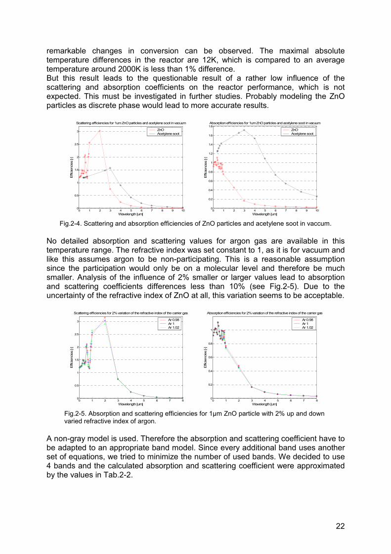
Analysis of variation of the process simulation caused by different absorption and scattering efficiencies are done. The data for acetylene soot was used for comparison. Although these values differ rather strongly (see Fig.2-4) for the calculated efficiencies with the extracted values for ZnO, the influence on the process simulation is rather small. Changes in efficiencies of less than 0.1% and no

22

remarkable changes in conversion can be observed. The maximal absolute temperature differences in the reactor are 12K, which is compared to an average temperature around 2000K is less than 1% difference. But this result leads to the questionable result of a rather low influence of the scattering and absorption coefficients on the reactor performance, which is not expected. This must be investigated in further studies. Probably modeling the ZnO particles as discrete phase would lead to more accurate results.

0 1 2 3 4 5 6 7 8 9 100

0.5

1

1.5

2

2.5

3

Wavelength [um]

Effi

cien

cies

[-]

Scattering efficiencies for 1um ZnO particles and acetylene soot in vacuum

ZnOAcetylene soot

0 1 2 3 4 5 6 7 8 9 100

0.2

0.4

0.6

0.8

1

1.2

1.4

1.6

1.8Absorption efficiencies for 1um ZnO particles and acetylene soot in vacuum

Wavelength [um]

Effi

cien

cies

[-]

ZnOAcetylene soot

Fig.2-4. Scattering and absorption efficiencies of ZnO particles and acetylene soot in vaccum. No detailed absorption and scattering values for argon gas are available in this temperature range. The refractive index was set constant to 1, as it is for vacuum and like this assumes argon to be non-participating. This is a reasonable assumption since the participation would only be on a molecular level and therefore be much smaller. Analysis of the influence of 2% smaller or larger values lead to absorption and scattering coefficients differences less than 10% (see Fig.2-5). Due to the uncertainty of the refractive index of ZnO at all, this variation seems to be acceptable.

0 1 2 3 4 5 6 7 80

0.5

1

1.5

2

2.5

3

Scattering efficiencies for 2% variation of the refractive index of the carrier gas

Wavelength [um]

Effi

cien

cies

[-]

Ar 0.98Ar 1Ar 1.02

0 1 2 3 4 5 6 7 80

0.2

0.4

0.6

0.8

1

Absorption efficiencies for 2% variation of the refractive index of the carrier gas

Wavelength [um]

Effi

cien

cies

[-]

Ar 0.98Ar 1Ar 1.02

Fig.2-5. Absorption and scattering efficiencies for 1µm ZnO particle with 2% up and down varied refractive index of argon.

A non-gray model is used. Therefore the absorption and scattering coefficient have to be adapted to an appropriate band model. Since every additional band uses another set of equations, we tried to minimize the number of used bands. We decided to use 4 bands and the calculated absorption and scattering coefficient were approximated by the values in Tab.2-2.

23

Band Absorption efficiencies [-] Scattering efficiencies [-] 0 – 1.0 µm 1 1.5 1.0 – 3.0 µm 0.5 3 3.0 – 7.0 µm 0.125 0.125 7.0 – 50’000 µm 0 0

2.2.a) Approximated efficiencies for a zinc-oxide particle with 1µm diameter in vacuum. Band Absorption efficiencies [-] Scattering efficiencies [-] 0 – 0.2 µm 1.5 1.2 0.2 – 0.4 µm 1.5 0.125 0.5 – 3.0 µm 0.0125 0.125 3.0 – 50’000 µm 0 02-2.b) Approximated efficiencies for a zinc-oxide particle with 0.06µm diameter in vacuum. Band 0-1.5µm 1.5-∞µm Incoming flux 3000 and 6000suns, respectively 0

Tab.2-3. Two band model used for the incoming radiation flux. When comparing a four band approximation and a two band approximation with averaged (grey) scattering and absorption coefficient of the core fluid, the difference in the temperature distribution in the reactor never exceeded more than 1K. Therefore the number of bands was reduced to two and like this the computational effort reduced by nearly a factor of two. By using two bands the incoming radiation from the sun, which has a peak in the ultraviolet region (see Fig.2-6), can still be modeled more accurately (see Tab.2-3) as well as the cavity wall reflectivity (see chapter 2.9).

0 0.2 0.4 0.6 0.8 1 1.2

x10-5

0

0.2

0.4

0.6

0.8

1

1.2

1.4

1.6

1.8

2x10

9

Wavelength [m]

Spe

ctra

linp

ut[W

/m3 ]

Ideal solar input on earth surface

Fig.2-6. Ideal solar spectral input on the earth surface. The sun is assumed to be a blackbody radiating at 5800K.

2.5. Models for gas diffusion

To account for the molecular mixing of different gases, diffusion coefficients must be calculated. For the case of a multicomponent mixture, diffusion coefficients of all involved gases within each other have to be calculated. In our case this would be 10 different diffusion coefficients (the ZnO particles are modeled as homogeneous gas cloud instead of discrete particles). But since we have a diluted mixture the dilute approximation can be assumed. Dilute approximation means the “bulk” media can be approximated by the gas, which is present in the largest amount (in our case the carrier gas argon) and the diffusion coefficient of the other gases can be calculated with respect to this gas. Therefore we need to calculate the diffusion coefficient of argon, zinc, zinc-oxide and oxygen in argon.

24

To account for the behavior of the zinc-oxide particle in the gas stream, its diffusion coefficient was set to 10-9 [14] since convection is more dominant than diffusion. To calculate the diffusion coefficient between two gases, several approaches exist. Either the Chapman-Enskog formula (2.38), which is derived by accounting for the molecular forces between molecules, can be used.

Ω⋅⋅

⋅⋅

+⋅

=

−

2

3

2/1

5.1 1086.111

σp

MMT

D yx (2.38)

Mx and My are the molar masses of the two gases in kg·kmol-1, σ the collision diameter in Å, Ω is the dimensionless collision integral. σ and Ω are molecular properties and can be looked up in tables [29, p.111]. They are derived from the Lenard-Jones potential between interacting atoms. There also exists an empirical formulation by Fuller (2.39), since the collision integral and the collision diameter are not known and calculable for all atoms and molecules. Instead of the molecular quantities σ and Ω, the so called diffusion volumes, v, are used. Data for the diffusion volumes can be found literature [29,30].

( )23/13/1

3

2/1

75.1 10013.111

yx

yx

vvp

MMT

D+⋅

⋅⋅

+⋅

=

−

(2.39)

Since for some molecules or atoms the molecular quantities and the diffusion volume is not known, other empirical relation of the form:

s

TTDD

+

=

1

00 (2.40)

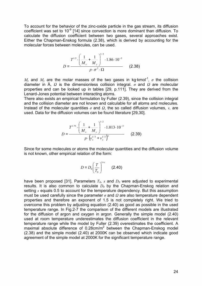
have been proposed [31]. Parameters T0, s and D0 were adjusted to experimental results. It is also common to calculate D0 by the Chapman-Enskog relation and setting s equals 0.5 to account for the temperature dependency. But this assumption must be used carefully since the parameter σ and Ω are also temperature dependent properties and therefore an exponent of 1.5 is not completely right. We tried to overcome this problem by adjusting equation (2.40) as good as possible in the used temperature range. In Fig.2-7 the comparison of the different models are illustrated for the diffusion of argon and oxygen in argon. Generally the simple model (2.40) used at room temperature underestimates the diffusion coefficient in the relevant temperature range while the model by Fuller (2.39) overestimates the coefficient. A maximal absolute difference of 0.28cm/m2 between the Chapman-Enskog model (2.38) and the simple model (2.40) at 2000K can be observed which indicate good agreement of the simple model at 2000K for the significant temperature range.

25

Comparison - Diffusion coefficient Ar in Ar

0

1

2

3

4

5

6

7

8

9

1600 1700 1800 1900 2000 2100 2200 2300 2400 2500 2600

T [K]

D[cm^2/s]

fullerchapman_enskogsimple_at293simple_at2000

Comparison - Diffusion coefficient of O2 in Ar

0

1

2

3

4

5

6

7

8

9

10

1800 1850 1900 1950 2000 2050 2100 2150 2200

T [K]

D[cm 2/s]

fullerchapman_enskogsimple_at293simple_at2000

Fig.2-7.a) Comparison of different models for the diffusion coefficient of argon in argon and b) of O2 in Ar. The models for Chapman-Enskog and Fuller are described by (2.38) and (2.39), respectively. Simple means the model described by (2.40) with s equals 0.5 and D0 calculated at either 293K or 2000K, respectively.

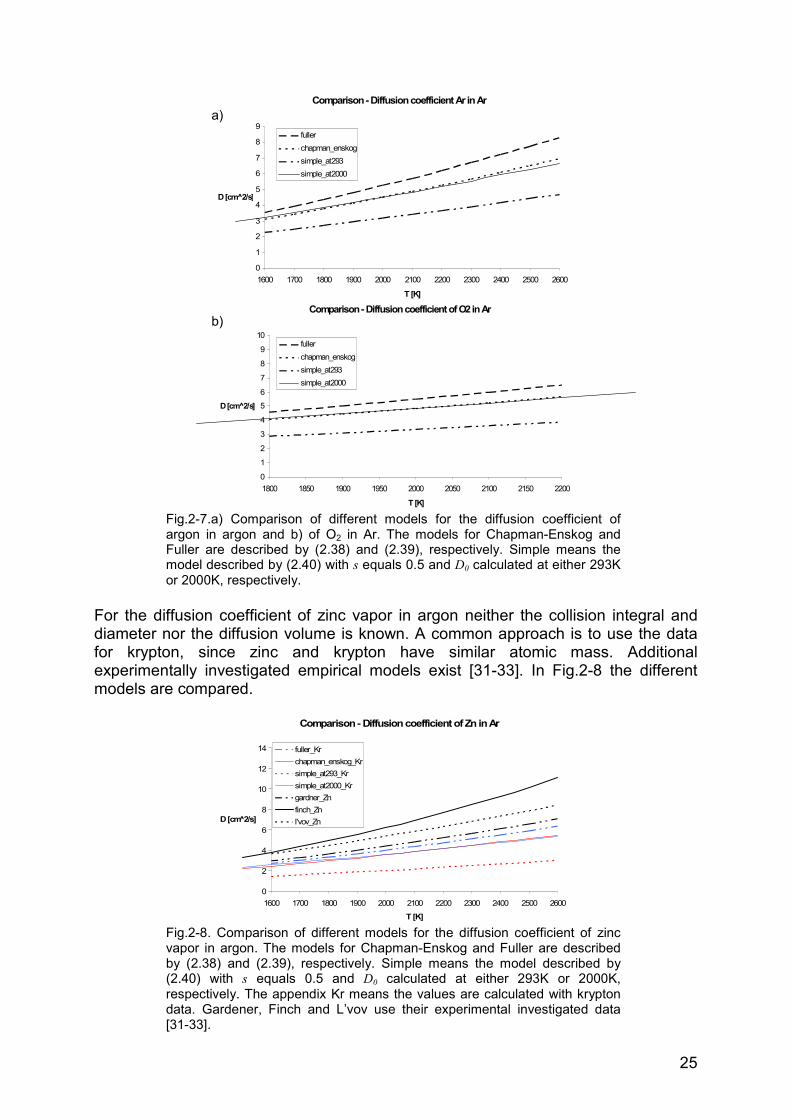
For the diffusion coefficient of zinc vapor in argon neither the collision integral and diameter nor the diffusion volume is known. A common approach is to use the data for krypton, since zinc and krypton have similar atomic mass. Additional experimentally investigated empirical models exist [31-33]. In Fig.2-8 the different models are compared.

Comparison - Diffusion coefficient of Zn in Ar

0

2

4

6

8

10

12

14

1600 1700 1800 1900 2000 2100 2200 2300 2400 2500 2600

T [K]

D[cm 2/s]

fuller_Krchapman_enskog_Krsimple_at293_Krsimple_at2000_Krgardner_Znfinch_Znl'vov_Zn

Fig.2-8. Comparison of different models for the diffusion coefficient of zinc vapor in argon. The models for Chapman-Enskog and Fuller are described by (2.38) and (2.39), respectively. Simple means the model described by (2.40) with s equals 0.5 and D0 calculated at either 293K or 2000K, respectively. The appendix Kr means the values are calculated with krypton data. Gardener, Finch and L’vov use their experimental investigated data [31-33].

a)

b)

26

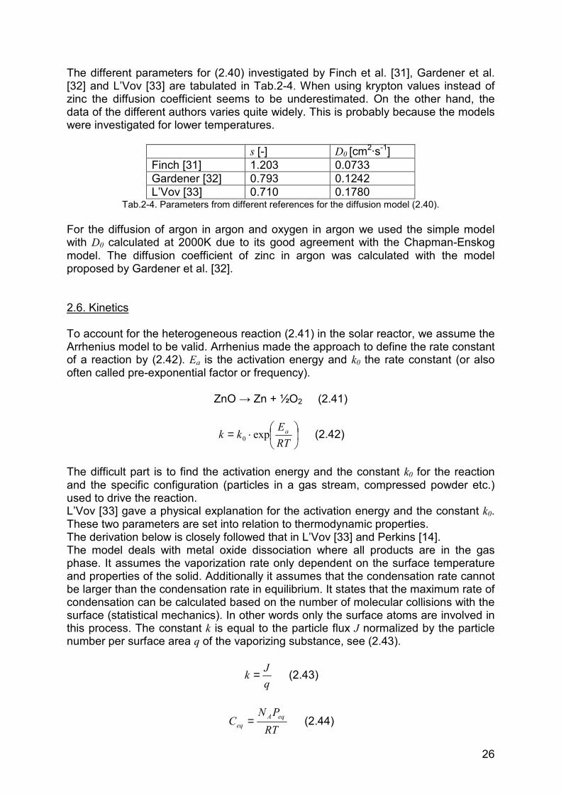
The different parameters for (2.40) investigated by Finch et al. [31], Gardener et al. [32] and L’Vov [33] are tabulated in Tab.2-4. When using krypton values instead of zinc the diffusion coefficient seems to be underestimated. On the other hand, the data of the different authors varies quite widely. This is probably because the models were investigated for lower temperatures.

s [-] D0 [cm2·s-1]Finch [31] 1.203 0.0733 Gardener [32] 0.793 0.1242 L’Vov [33] 0.710 0.1780

Tab.2-4. Parameters from different references for the diffusion model (2.40). For the diffusion of argon in argon and oxygen in argon we used the simple model with D0 calculated at 2000K due to its good agreement with the Chapman-Enskog model. The diffusion coefficient of zinc in argon was calculated with the model proposed by Gardener et al. [32].

2.6. Kinetics

To account for the heterogeneous reaction (2.41) in the solar reactor, we assume the Arrhenius model to be valid. Arrhenius made the approach to define the rate constant of a reaction by (2.42). Ea is the activation energy and k0 the rate constant (or also often called pre-exponential factor or frequency).

ZnO → Zn + ½O2 (2.41)

⋅=RTEkk aexp0 (2.42)

The difficult part is to find the activation energy and the constant k0 for the reaction and the specific configuration (particles in a gas stream, compressed powder etc.) used to drive the reaction. L’Vov [33] gave a physical explanation for the activation energy and the constant k0.These two parameters are set into relation to thermodynamic properties. The derivation below is closely followed that in L’Vov [33] and Perkins [14]. The model deals with metal oxide dissociation where all products are in the gas phase. It assumes the vaporization rate only dependent on the surface temperature and properties of the solid. Additionally it assumes that the condensation rate cannot be larger than the condensation rate in equilibrium. It states that the maximum rate of condensation can be calculated based on the number of molecular collisions with the surface (statistical mechanics). In other words only the surface atoms are involved in this process. The constant k is equal to the particle flux J normalized by the particle number per surface area q of the vaporizing substance, see (2.43).

qJk = (2.43)

RTPN

C eqAeq = (2.44)

27

cDJ ∇⋅−= (2.45) Using the Clapyron-Mendeleev equation (2.44) and Fick’s first law (2.45) we can express the particle flux J and like this also k in a new way:

qzRTDPN

k eqA= (2.46)

where NA is the Avogadro constant, D the diffusion coefficient, z the distance of the vaporization surface to the sink and Peq the equilibrium pressure. Now assuming a reaction of the form (2.47), the pressure defined equilibrium constant can be given by (2.48) and equilibrium partial pressures can be expressed with the diffusion constants (2.49).

)()()( gbOgaMsOM ba +→ (2.47)

bO

aMp PPK = (2.48)

M

O

O

M

DD

ba

PP

= (2.49)

DO is the diffusion constant of the oxygen in the phase and DM the diffusion coefficient of the metal vapor in the phase. Additionally using the Gibbs free energy relation:

000)ln( TTTp STHGKRT ∆⋅−∆=∆=− (2.50) We can rewrite (2.46) in the following form:

+

∆⋅

+

∆⋅

=

+

+)(

exp)(

exp)(

00

1 baRTH

baRS

DD

ba

aDqzRTNk TT

bab

M

O

babaM

A (2.51)

By comparing the equation with equation (2.42), we can now extract the activation energy Ea as well as the rate constant k0.

baHE T

a +∆

=0

(2.52)

+

∆⋅

=

+

+)(

exp)(

0

10 baRS

DD

ba

aDqzRTNk T

bab

M

O

babaM

A (2.53)

The activation energy Ea can be physically interpreted as the enthalpy of reaction or the enthalpy of vaporization divided by the stoechiometric constants of the reaction. The constant k0 is characterized by a product of the transport of the particle (part of the term with the diffusion constant) and the entropy change.

28

k0 [s-1]Minimal value 2.23·109

Maximal value 1.76·1010

Tab.2-5. Minimal and maximal values of the experimentally investigated pre-exponential factor by Perkins [14].

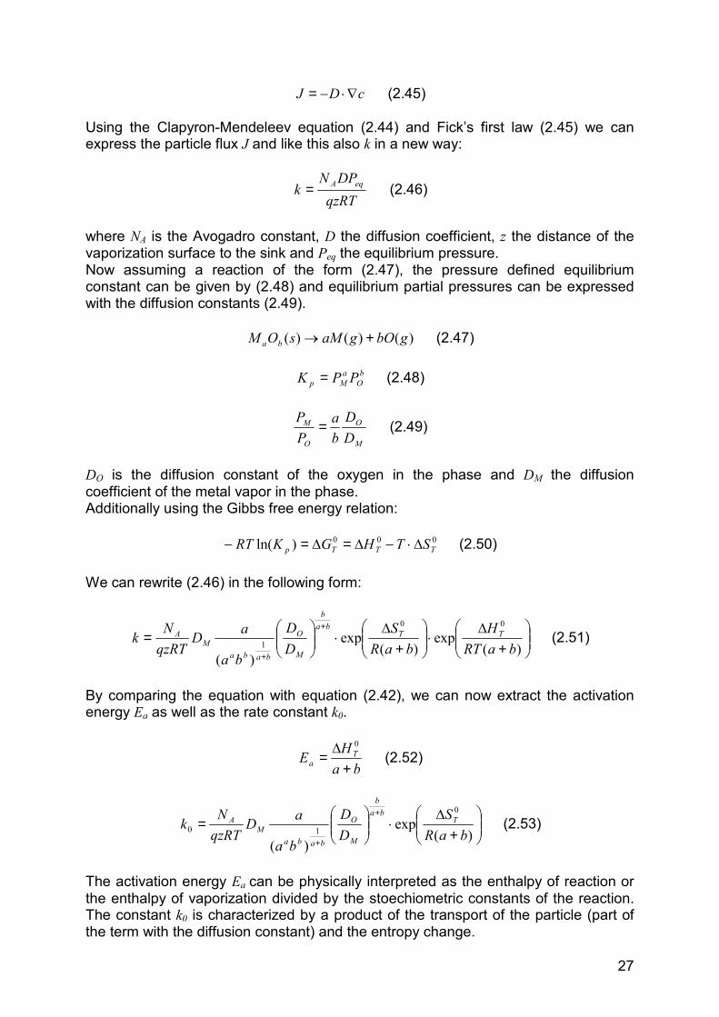
Another difficulty is to define the distance z for our reactor design. Perkins [14] investigated them experimentally (see Tab.2-5). Since the experimentally investigated results have a relatively high variation, the influence of this variation on the theoretical calculated efficiencies is analyzed. Variations of the pre-exponential factor in the range of 2.23e9-1.67e10s-1 lead to efficiency variations of 2%, conversion variations of 12% and temperature variations of 7%. We conclude that these variations are acceptable. The dissociation of zinc-oxide to zinc vapor and oxygen has a reaction enthalpy of 470kJ/mol. Perkins [14] showed that the reaction (2.54) is the rate limiting step.

ZnO → Zn + O (2.54) Therefore the activation energy according to this reaction is calculated. It is calculated and also experimentally validated to be 356kJ/mol [14]. Formulation (2.53) leads to the conclusion of a weak temperature dependence of the constant k0, since the temperature in the denominator is nearly offset by the temperature dependency of the diffusion constants. Therefore the reaction constant can be assumed temperature independent in a small temperature range (see Fig.2-9).

k0 as function of temperature

0.00E+00

1.00E+10

2.00E+10

3.00E+10

4.00E+10

1800 1850 1900 1950 2000 2050 2100 2150 2200 2250 2300

T [K]

k0 [1/s]

Fig.2-9. k0 calculated with (2.53) in the temperature range of 1800 to 2300K. z was set to 1µm.

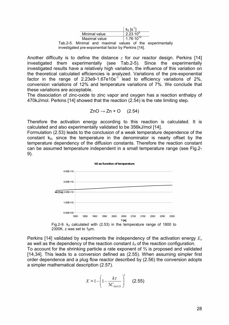
Perkins [14] validated by experiments the independency of the activation energy Eaas well as the dependency of the reaction constant k0 of the reaction configuration. To account for the shrinking particle a rate exponent of ⅔ is proposed and validated [14,34]. This leads to a conversion defined as (2.55). When assuming simpler first order dependence and a plug flow reactor described by (2.56) the conversion adopts a simpler mathematical description (2.57).

3

0,311

−−=

ZnOCkX τ (2.55)

29

∫∫ −=

X

ZnOZnO

V

rdXndV

00,

0

& (2.56)

)exp(1 τ⋅−−= kX (2.57)

rZnO is the reaction rate, X the conversion, 0,ZnOn& the initial molar rate of zinc-oxide, kthe rate constant, V the reactor volume and τ the resident time defined as the fraction of reaction volume to volumetric rate. Due to simplification and since variation in the pre-exponential factor leads to much larger change in conversion than changes due to variation in the rate exponent (see Fig.2-10) a rate exponent of 1 was used in the work at hand.

Different conversion models

0

0.1

0.2

0.3

0.4

0.5

0.6

0.7

0.8

0.9

1

1300 1500 1700 1900 2100 2300 2500T [K]

X [-]

k_min_2/3k_min_1k_max_2/3k_max_1

Fig.2-10. Conversion calculated with different rate exponents (⅔ and 1) and the extreme values for the pre-exponential factor.

2.7. Thermophysical properties

The thermophysical properties of zinc vapour, oxygen, zinc-oxide, argon and air are needed for the fluid phase in the simulation. For the solid phases the properties of silicon-carbide, alumina and quartz are needed. The gaseous materials are modelled as ideal gases. The ideal gas approximation ignores the self volume of the gas and also the interactions between the molecules. Detailed comparison of the ideal gas model with the real gas model of Redlich-Kwong (an empirical upgrade of the Van-der-Waals model) is done by [15]. In the relevant temperature range the two models are nearly identical. Therefore the ideal gas model is a good assumption. Since temperature dependent properties not only improve accuracy but also lead to faster convergence behaviour the properties for the materials are used temperature dependent, if available. The properties of the gaseous materials are taken from [35,36] and are given in Tab.2-6. The difficulty is to find values for the zinc-oxide properties since only few data is available and since the zinc-oxide particles are modelled as homogeneous gas cloud. Its thermal conductivity was taken from [37] and for the viscosity a common value for gaseous species is assumed due to lack of data. The density was used of solid zinc-oxide put scaled with the volume fraction of the zinc-oxide [14]. The mixture of the gases is modelled as ideal mixture, which means that the properties of the mixture are calculated directly from the properties of its components and their proportions (mass fraction) in the mixture.

30

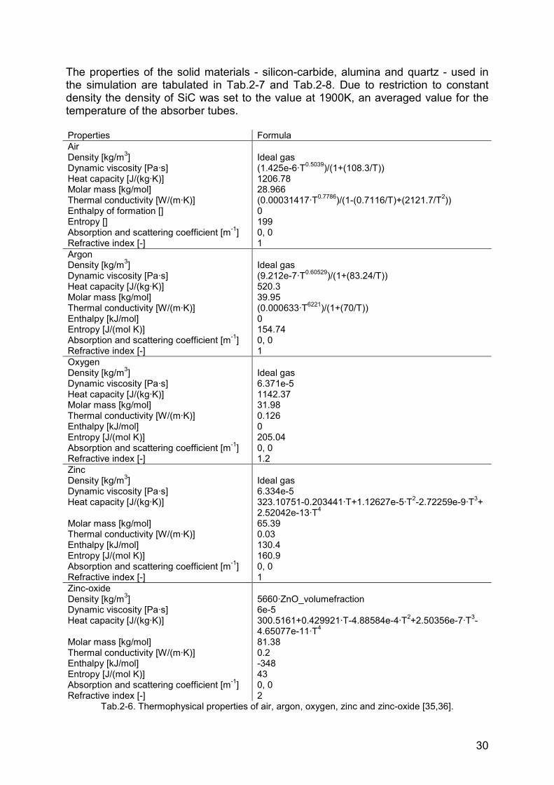
The properties of the solid materials - silicon-carbide, alumina and quartz - used in the simulation are tabulated in Tab.2-7 and Tab.2-8. Due to restriction to constant density the density of SiC was set to the value at 1900K, an averaged value for the temperature of the absorber tubes. Properties Formula Air Density [kg/m3]Dynamic viscosity [Pa·s] Heat capacity [J/(kg·K)] Molar mass [kg/mol] Thermal conductivity [W/(m·K)] Enthalpy of formation [] Entropy [] Absorption and scattering coefficient [m-1]Refractive index [-]

Ideal gas (1.425e-6·T0.5039)/(1+(108.3/T)) 1206.78 28.966 (0.00031417·T0.7786)/(1-(0.7116/T)+(2121.7/T2)) 0199 0, 0 1

Argon Density [kg/m3]Dynamic viscosity [Pa·s] Heat capacity [J/(kg·K)] Molar mass [kg/mol] Thermal conductivity [W/(m·K)] Enthalpy [kJ/mol] Entropy [J/(mol K)] Absorption and scattering coefficient [m-1]Refractive index [-]

Ideal gas (9.212e-7·T0.60529)/(1+(83.24/T)) 520.3 39.95 (0.000633·T6221)/(1+(70/T)) 0154.74 0, 0 1

Oxygen Density [kg/m3]Dynamic viscosity [Pa·s] Heat capacity [J/(kg·K)] Molar mass [kg/mol] Thermal conductivity [W/(m·K)] Enthalpy [kJ/mol] Entropy [J/(mol K)] Absorption and scattering coefficient [m-1]Refractive index [-]

Ideal gas 6.371e-5 1142.37 31.98 0.126 0205.04 0, 0 1.2

Zinc Density [kg/m3]Dynamic viscosity [Pa·s] Heat capacity [J/(kg·K)] Molar mass [kg/mol] Thermal conductivity [W/(m·K)] Enthalpy [kJ/mol] Entropy [J/(mol K)] Absorption and scattering coefficient [m-1]Refractive index [-]

Ideal gas 6.334e-5 323.10751-0.203441·T+1.12627e-5·T2-2.72259e-9·T3+2.52042e-13·T4

65.39 0.03 130.4 160.9 0, 0 1

Zinc-oxide Density [kg/m3]Dynamic viscosity [Pa·s] Heat capacity [J/(kg·K)] Molar mass [kg/mol] Thermal conductivity [W/(m·K)] Enthalpy [kJ/mol] Entropy [J/(mol K)] Absorption and scattering coefficient [m-1]Refractive index [-]

5660·ZnO_volumefraction 6e-5 300.5161+0.429921·T-4.88584e-4·T2+2.50356e-7·T3-4.65077e-11·T4

81.38 0.2 -348 43 0, 0 2

Tab.2-6. Thermophysical properties of air, argon, oxygen, zinc and zinc-oxide [35,36].

31

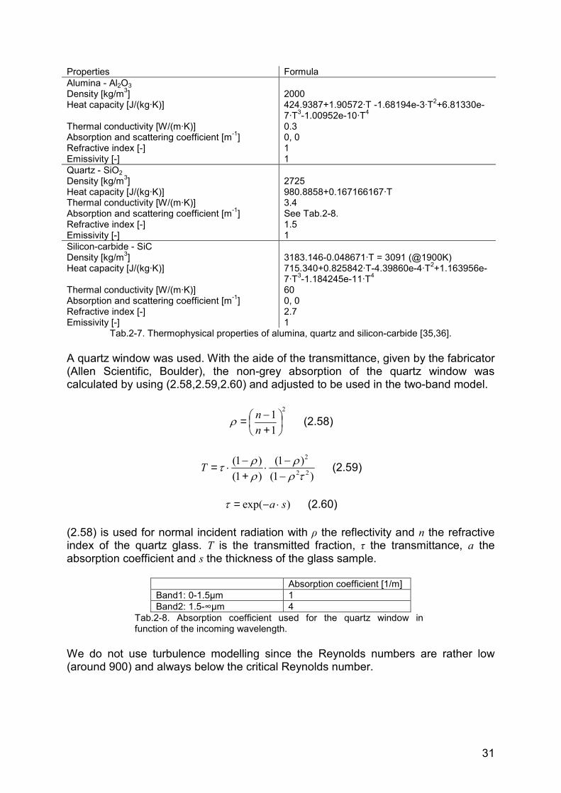
Properties Formula Alumina - Al2O3Density [kg/m3]Heat capacity [J/(kg·K)] Thermal conductivity [W/(m·K)] Absorption and scattering coefficient [m-1]Refractive index [-] Emissivity [-]

2000 424.9387+1.90572·T -1.68194e-3·T2+6.81330e-7·T3-1.00952e-10·T4

0.3 0, 0 11

Quartz - SiO2Density [kg/m3]Heat capacity [J/(kg·K)] Thermal conductivity [W/(m·K)] Absorption and scattering coefficient [m-1]Refractive index [-] Emissivity [-]

2725 980.8858+0.167166167·T 3.4 See Tab.2-8. 1.5 1

Silicon-carbide - SiC Density [kg/m3]Heat capacity [J/(kg·K)] Thermal conductivity [W/(m·K)] Absorption and scattering coefficient [m-1]Refractive index [-] Emissivity [-]

3183.146-0.048671·T = 3091 (@1900K) 715.340+0.825842·T-4.39860e-4·T2+1.163956e-7·T3-1.184245e-11·T4

60 0, 0 2.7 1

Tab.2-7. Thermophysical properties of alumina, quartz and silicon-carbide [35,36]. A quartz window was used. With the aide of the transmittance, given by the fabricator (Allen Scientific, Boulder), the non-grey absorption of the quartz window was calculated by using (2.58,2.59,2.60) and adjusted to be used in the two-band model.

2

11

+−=

nnρ (2.58)

)1()1(

)1()1(

22

2

τρρ

ρρτ

−−

⋅+−

⋅=T (2.59)

)exp( sa ⋅−=τ (2.60)

(2.58) is used for normal incident radiation with ρ the reflectivity and n the refractive index of the quartz glass. T is the transmitted fraction, τ the transmittance, a the absorption coefficient and s the thickness of the glass sample.

Absorption coefficient [1/m] Band1: 0-1.5µm 1 Band2: 1.5-∞µm 4

Tab.2-8. Absorption coefficient used for the quartz window in function of the incoming wavelength.

We do not use turbulence modelling since the Reynolds numbers are rather low (around 900) and always below the critical Reynolds number.

32

2.8. Geometry

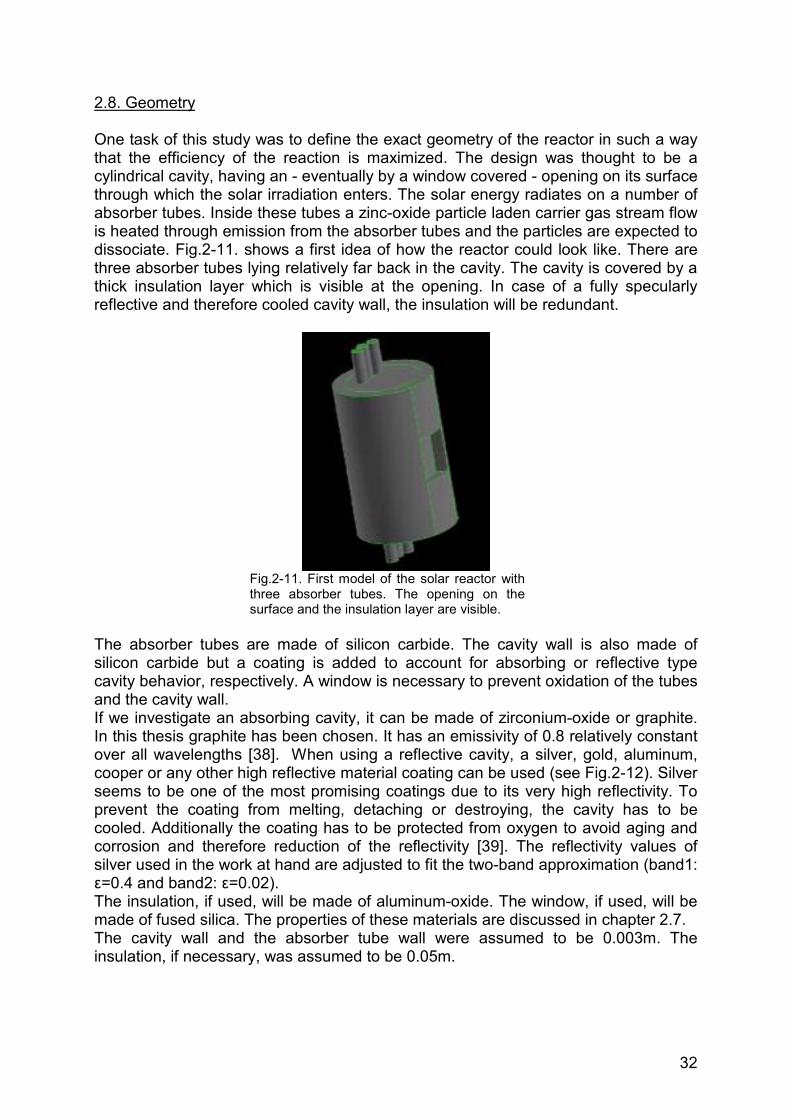
One task of this study was to define the exact geometry of the reactor in such a way that the efficiency of the reaction is maximized. The design was thought to be a cylindrical cavity, having an - eventually by a window covered - opening on its surface through which the solar irradiation enters. The solar energy radiates on a number of absorber tubes. Inside these tubes a zinc-oxide particle laden carrier gas stream flow is heated through emission from the absorber tubes and the particles are expected to dissociate. Fig.2-11. shows a first idea of how the reactor could look like. There are three absorber tubes lying relatively far back in the cavity. The cavity is covered by a thick insulation layer which is visible at the opening. In case of a fully specularly reflective and therefore cooled cavity wall, the insulation will be redundant.

Fig.2-11. First model of the solar reactor with three absorber tubes. The opening on the surface and the insulation layer are visible.

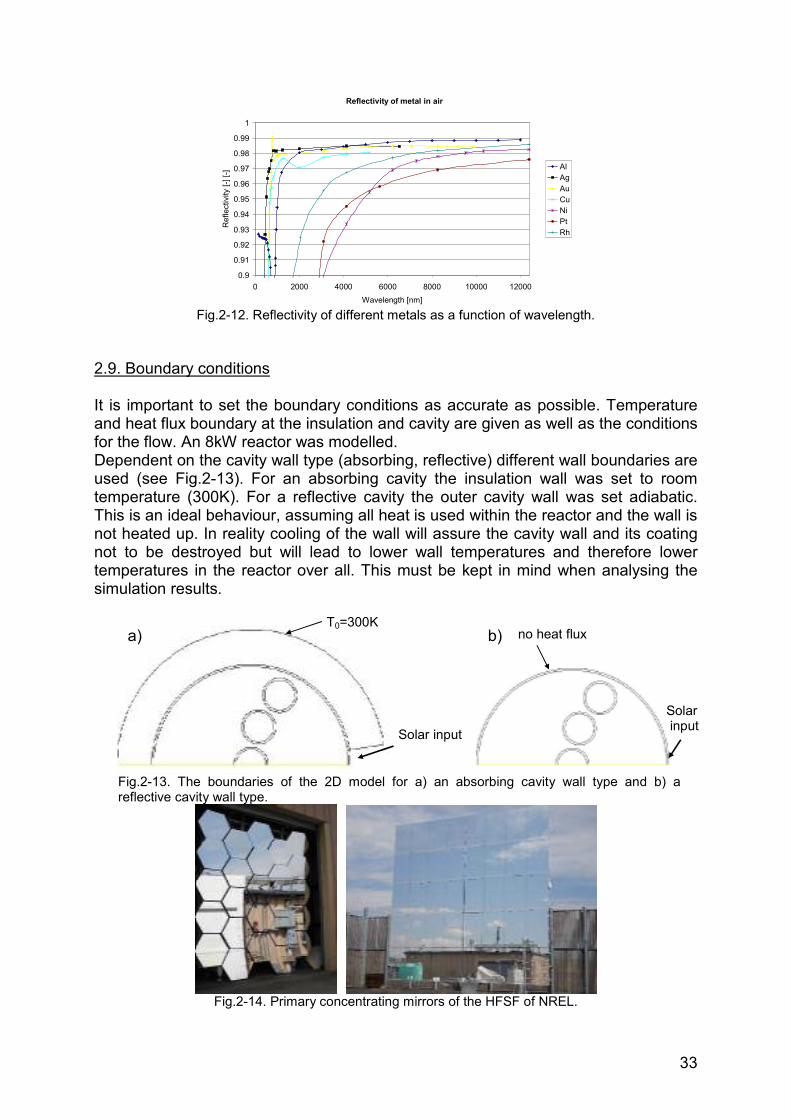
The absorber tubes are made of silicon carbide. The cavity wall is also made of silicon carbide but a coating is added to account for absorbing or reflective type cavity behavior, respectively. A window is necessary to prevent oxidation of the tubes and the cavity wall. If we investigate an absorbing cavity, it can be made of zirconium-oxide or graphite. In this thesis graphite has been chosen. It has an emissivity of 0.8 relatively constant over all wavelengths [38]. When using a reflective cavity, a silver, gold, aluminum, cooper or any other high reflective material coating can be used (see Fig.2-12). Silver seems to be one of the most promising coatings due to its very high reflectivity. To prevent the coating from melting, detaching or destroying, the cavity has to be cooled. Additionally the coating has to be protected from oxygen to avoid aging and corrosion and therefore reduction of the reflectivity [39]. The reflectivity values of silver used in the work at hand are adjusted to fit the two-band approximation (band1: ε=0.4 and band2: ε=0.02). The insulation, if used, will be made of aluminum-oxide. The window, if used, will be made of fused silica. The properties of these materials are discussed in chapter 2.7. The cavity wall and the absorber tube wall were assumed to be 0.003m. The insulation, if necessary, was assumed to be 0.05m.

33

Reflectivity of metal in air

0.9

0.91

0.92

0.93

0.94

0.95

0.96

0.97

0.98

0.99

1

0 2000 4000 6000 8000 10000 12000Wavelength [nm]

Ref

lect

ivity

[-][-]

AlAgAuCuNiPtRh

Fig.2-12. Reflectivity of different metals as a function of wavelength.

2.9. Boundary conditions

It is important to set the boundary conditions as accurate as possible. Temperature and heat flux boundary at the insulation and cavity are given as well as the conditions for the flow. An 8kW reactor was modelled. Dependent on the cavity wall type (absorbing, reflective) different wall boundaries are used (see Fig.2-13). For an absorbing cavity the insulation wall was set to room temperature (300K). For a reflective cavity the outer cavity wall was set adiabatic. This is an ideal behaviour, assuming all heat is used within the reactor and the wall is not heated up. In reality cooling of the wall will assure the cavity wall and its coating not to be destroyed but will lead to lower wall temperatures and therefore lower temperatures in the reactor over all. This must be kept in mind when analysing the simulation results.

Fig.2-13. The boundaries of the 2D model for a) an absorbing cavity wall type and b) a reflective cavity wall type.

Fig.2-14. Primary concentrating mirrors of the HFSF of NREL.

a) b) T0=300K

no heat flux

Solar input

Solar input

34

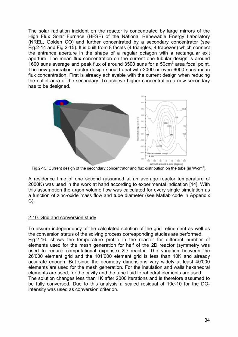
The solar radiation incident on the reactor is concentrated by large mirrors of the High Flux Solar Furnace (HFSF) of the National Renewable Energy Laboratory (NREL, Golden CO) and further concentrated by a secondary concentrator (see Fig.2-14 and Fig.2-15). It is built from 8 facets (4 triangles, 4 trapezes) which connect the entrance aperture in the shape of a regular octagon with a rectangular exit aperture. The mean flux concentration on the current one tubular design is around 1600 suns average and peak flux of around 3500 suns for a 50cm2 area focal point. The new generation reactor design should deal with 3000 or even 6000 suns mean flux concentration. First is already achievable with the current design when reducing the outlet area of the secondary. To achieve higher concentration a new secondary has to be designed.

Fig.2-15. Current design of the secondary concentrator and flux distribution on the tube (in W/cm2). A residence time of one second (assumed at an average reactor temperature of 2000K) was used in the work at hand according to experimental indication [14]. With this assumption the argon volume flow was calculated for every single simulation as a function of zinc-oxide mass flow and tube diameter (see Matlab code in Appendix C).

2.10. Grid and conversion study

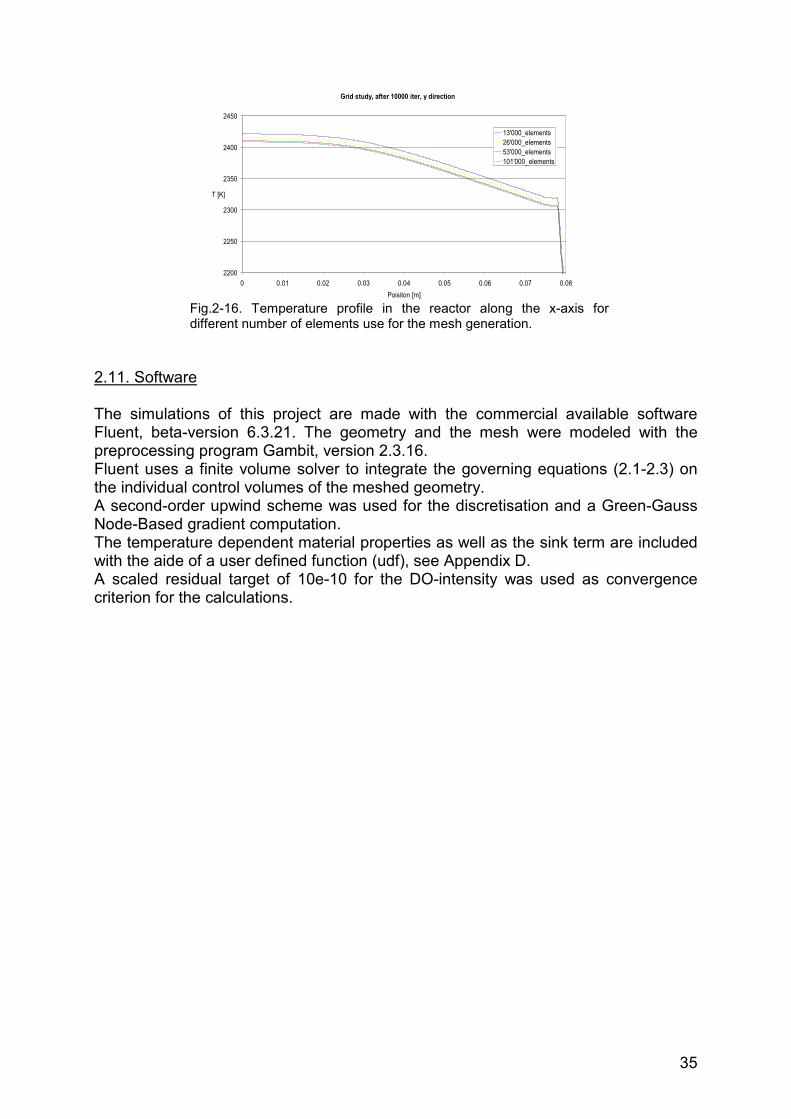
To assure independency of the calculated solution of the grid refinement as well as the conversion status of the solving process corresponding studies are performed. Fig.2-16. shows the temperature profile in the reactor for different number of elements used for the mesh generation for half of the 2D reactor (symmetry was used to reduce computational expense) 2D reactor. The variation between the 26’000 element grid and the 101’000 element grid is less than 10K and already accurate enough. But since the geometry dimensions vary widely at least 40’000 elements are used for the mesh generation. For the insulation and walls hexahedral elements are used, for the cavity and the tube fluid tetrahedral elements are used. The solution changes less than 1K after 2000 iterations and is therefore assumed to be fully conversed. Due to this analysis a scaled residual of 10e-10 for the DO-intensity was used as conversion criterion.

35

Grid study, after 10000 iter, y direction

2200

2250

2300

2350

2400

2450

0 0.01 0.02 0.03 0.04 0.05 0.06 0.07 0.08Poisiton [m]

T [K]

13'000_elements26'000_elements53'000_elements101'000_elements

Fig.2-16. Temperature profile in the reactor along the x-axis for different number of elements use for the mesh generation.

2.11. Software

The simulations of this project are made with the commercial available software Fluent, beta-version 6.3.21. The geometry and the mesh were modeled with the preprocessing program Gambit, version 2.3.16. Fluent uses a finite volume solver to integrate the governing equations (2.1-2.3) on the individual control volumes of the meshed geometry. A second-order upwind scheme was used for the discretisation and a Green-Gauss Node-Based gradient computation. The temperature dependent material properties as well as the sink term are included with the aide of a user defined function (udf), see Appendix D. A scaled residual target of 10e-10 for the DO-intensity was used as convergence criterion for the calculations.

36

3. Results 2D simulations

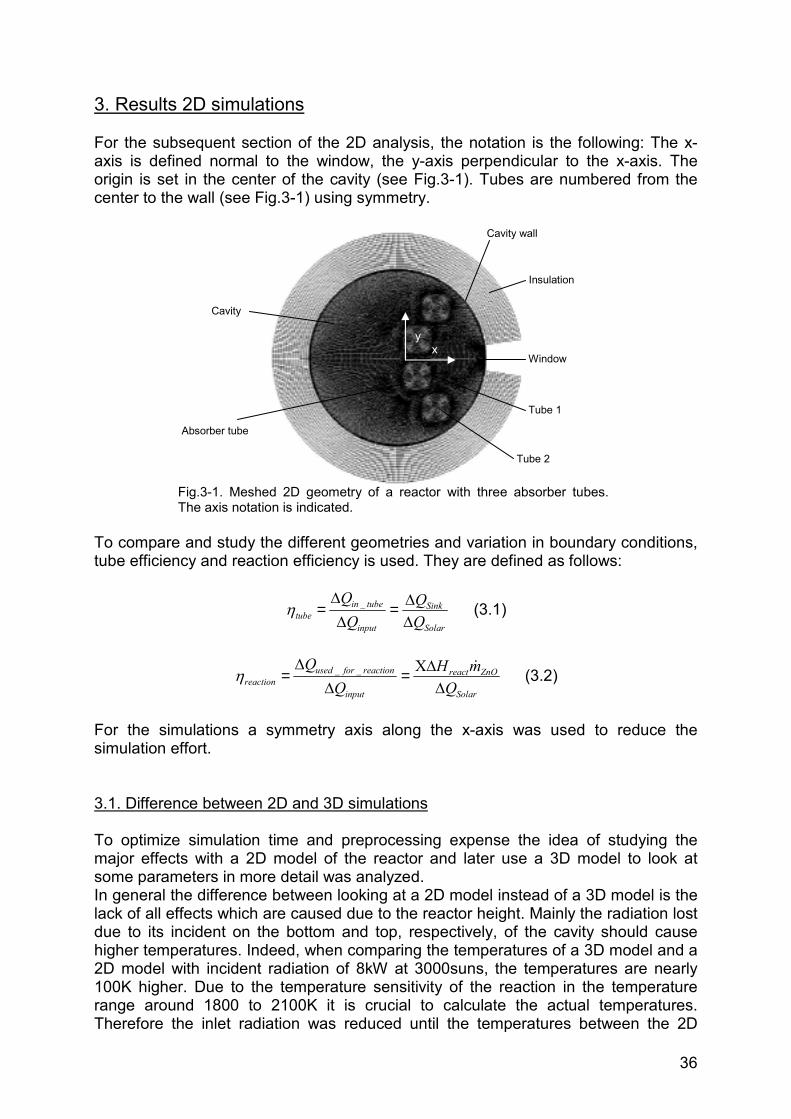
For the subsequent section of the 2D analysis, the notation is the following: The x-axis is defined normal to the window, the y-axis perpendicular to the x-axis. The origin is set in the center of the cavity (see Fig.3-1). Tubes are numbered from the center to the wall (see Fig.3-1) using symmetry.

Fig.3-1. Meshed 2D geometry of a reactor with three absorber tubes. The axis notation is indicated.

To compare and study the different geometries and variation in boundary conditions, tube efficiency and reaction efficiency is used. They are defined as follows:

Solar

Sink

input

tubeintube Q

QQ

Q∆∆=

∆∆

= _η (3.1)

Solar

ZnOreact

input

reactionforusedreaction Q

mHQ

Q∆

Χ∆=∆

∆=

&__η (3.2)

For the simulations a symmetry axis along the x-axis was used to reduce the simulation effort.

3.1. Difference between 2D and 3D simulations

To optimize simulation time and preprocessing expense the idea of studying the major effects with a 2D model of the reactor and later use a 3D model to look at some parameters in more detail was analyzed. In general the difference between looking at a 2D model instead of a 3D model is the lack of all effects which are caused due to the reactor height. Mainly the radiation lost due to its incident on the bottom and top, respectively, of the cavity should cause higher temperatures. Indeed, when comparing the temperatures of a 3D model and a 2D model with incident radiation of 8kW at 3000suns, the temperatures are nearly 100K higher. Due to the temperature sensitivity of the reaction in the temperature range around 1800 to 2100K it is crucial to calculate the actual temperatures. Therefore the inlet radiation was reduced until the temperatures between the 2D

yx

Cavity wall

Insulation

Absorber tube

Cavity

Window

Tube 1

Tube 2

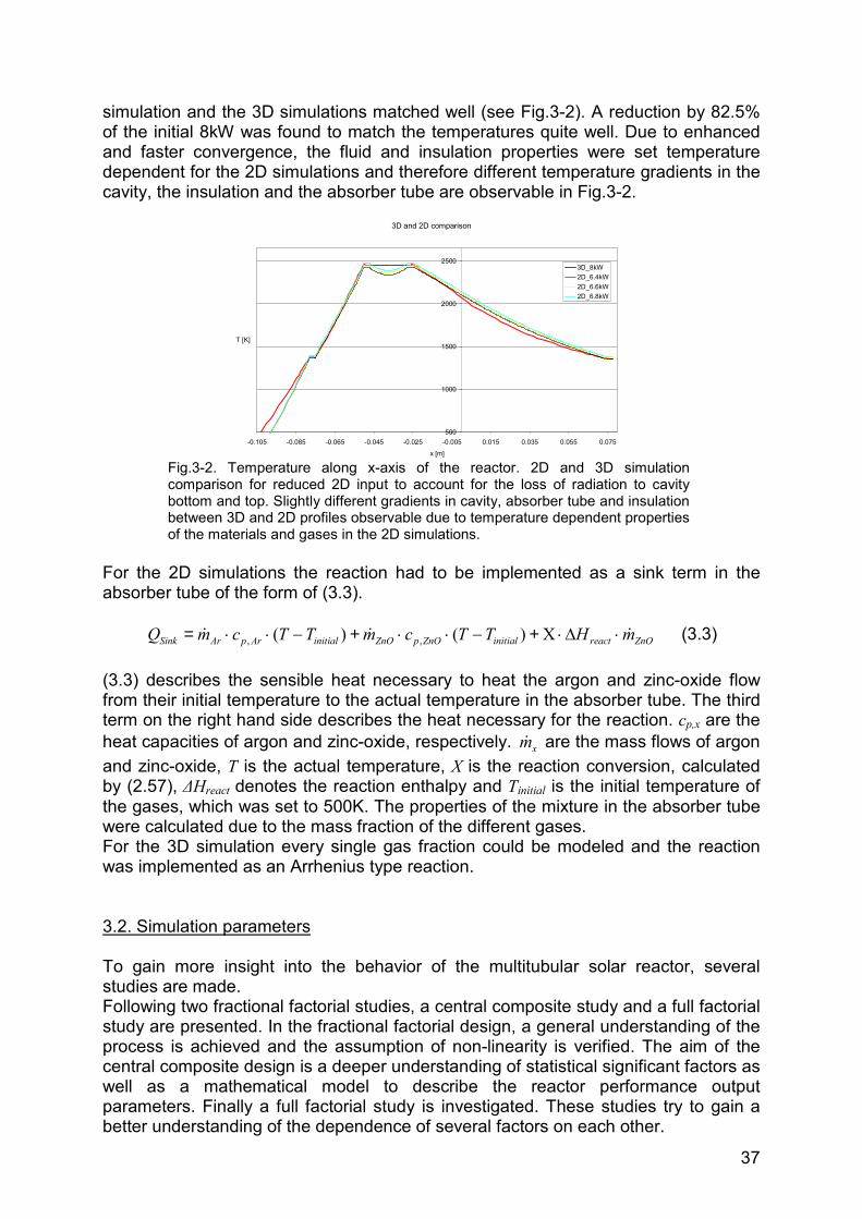
37

simulation and the 3D simulations matched well (see Fig.3-2). A reduction by 82.5% of the initial 8kW was found to match the temperatures quite well. Due to enhanced and faster convergence, the fluid and insulation properties were set temperature dependent for the 2D simulations and therefore different temperature gradients in the cavity, the insulation and the absorber tube are observable in Fig.3-2.

3D and 2D comparison

500

1000

1500

2000

2500

-0.105 -0.085 -0.065 -0.045 -0.025 -0.005 0.015 0.035 0.055 0.075

x [m]

T [K]

3D_8kW2D_6.4kW2D_6.6kW2D_6.8kW

Fig.3-2. Temperature along x-axis of the reactor. 2D and 3D simulation comparison for reduced 2D input to account for the loss of radiation to cavity bottom and top. Slightly different gradients in cavity, absorber tube and insulation between 3D and 2D profiles observable due to temperature dependent properties of the materials and gases in the 2D simulations.

For the 2D simulations the reaction had to be implemented as a sink term in the absorber tube of the form of (3.3).

ZnOreactinitialZnOpZnOinitialArpArSink mHTTcmTTcmQ &&& ⋅∆⋅Χ+−⋅⋅+−⋅⋅= )()( ,, (3.3)

(3.3) describes the sensible heat necessary to heat the argon and zinc-oxide flow from their initial temperature to the actual temperature in the absorber tube. The third term on the right hand side describes the heat necessary for the reaction. cp,x are the heat capacities of argon and zinc-oxide, respectively. xm& are the mass flows of argon and zinc-oxide, T is the actual temperature, Χ is the reaction conversion, calculated by (2.57), ∆Hreact denotes the reaction enthalpy and Tinitial is the initial temperature of the gases, which was set to 500K. The properties of the mixture in the absorber tube were calculated due to the mass fraction of the different gases. For the 3D simulation every single gas fraction could be modeled and the reaction was implemented as an Arrhenius type reaction.

3.2. Simulation parameters

To gain more insight into the behavior of the multitubular solar reactor, several studies are made. Following two fractional factorial studies, a central composite study and a full factorial study are presented. In the fractional factorial design, a general understanding of the process is achieved and the assumption of non-linearity is verified. The aim of the central composite design is a deeper understanding of statistical significant factors as well as a mathematical model to describe the reactor performance output parameters. Finally a full factorial study is investigated. These studies try to gain a better understanding of the dependence of several factors on each other.

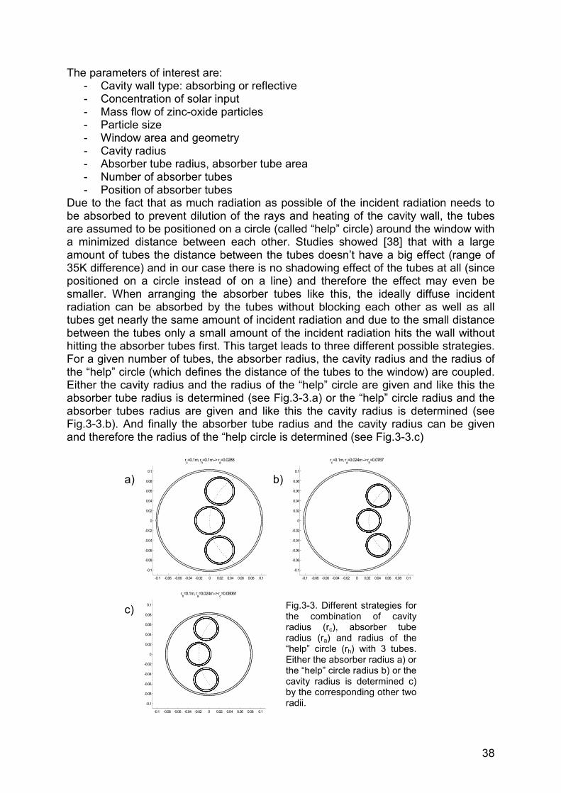
38

The parameters of interest are: - Cavity wall type: absorbing or reflective - Concentration of solar input - Mass flow of zinc-oxide particles - Particle size - Window area and geometry - Cavity radius - Absorber tube radius, absorber tube area - Number of absorber tubes - Position of absorber tubes

Due to the fact that as much radiation as possible of the incident radiation needs to be absorbed to prevent dilution of the rays and heating of the cavity wall, the tubes are assumed to be positioned on a circle (called “help” circle) around the window with a minimized distance between each other. Studies showed [38] that with a large amount of tubes the distance between the tubes doesn’t have a big effect (range of 35K difference) and in our case there is no shadowing effect of the tubes at all (since positioned on a circle instead of on a line) and therefore the effect may even be smaller. When arranging the absorber tubes like this, the ideally diffuse incident radiation can be absorbed by the tubes without blocking each other as well as all tubes get nearly the same amount of incident radiation and due to the small distance between the tubes only a small amount of the incident radiation hits the wall without hitting the absorber tubes first. This target leads to three different possible strategies. For a given number of tubes, the absorber radius, the cavity radius and the radius of the “help” circle (which defines the distance of the tubes to the window) are coupled. Either the cavity radius and the radius of the “help” circle are given and like this the absorber tube radius is determined (see Fig.3-3.a) or the “help” circle radius and the absorber tubes radius are given and like this the cavity radius is determined (see Fig.3-3.b). And finally the absorber tube radius and the cavity radius can be given and therefore the radius of the “help circle is determined (see Fig.3-3.c)

-0.1 -0.08 -0.06 -0.04 -0.02 0 0.02 0.04 0.06 0.08 0.1

-0.1

-0.08

-0.06

-0.04

-0.02

0

0.02

0.04

0.06

0.08

0.1

rc=0.1m, rh=0.1m -> ra=0.0288

-0.1 -0.08 -0.06 -0.04 -0.02 0 0.02 0.04 0.06 0.08 0.1

-0.1

-0.08

-0.06

-0.04

-0.02

0

0.02

0.04

0.06

0.08

0.1

rc=0.1m, ra=0.024m -> rh=0.0767

-0.1 -0.08 -0.06 -0.04 -0.02 0 0.02 0.04 0.06 0.08 0.1

-0.1

-0.08

-0.06

-0.04

-0.02

0

0.02

0.04

0.06

0.08

0.1

rh=0.1m, ra=0.024m -> rc=0.08061

a) b)

c)

Fig.3-3. Different strategies for the combination of cavity radius (rc), absorber tube radius (ra) and radius of the “help” circle (rh) with 3 tubes. Either the absorber radius a) or the “help” circle radius b) or the cavity radius is determined c) by the corresponding other two radii.

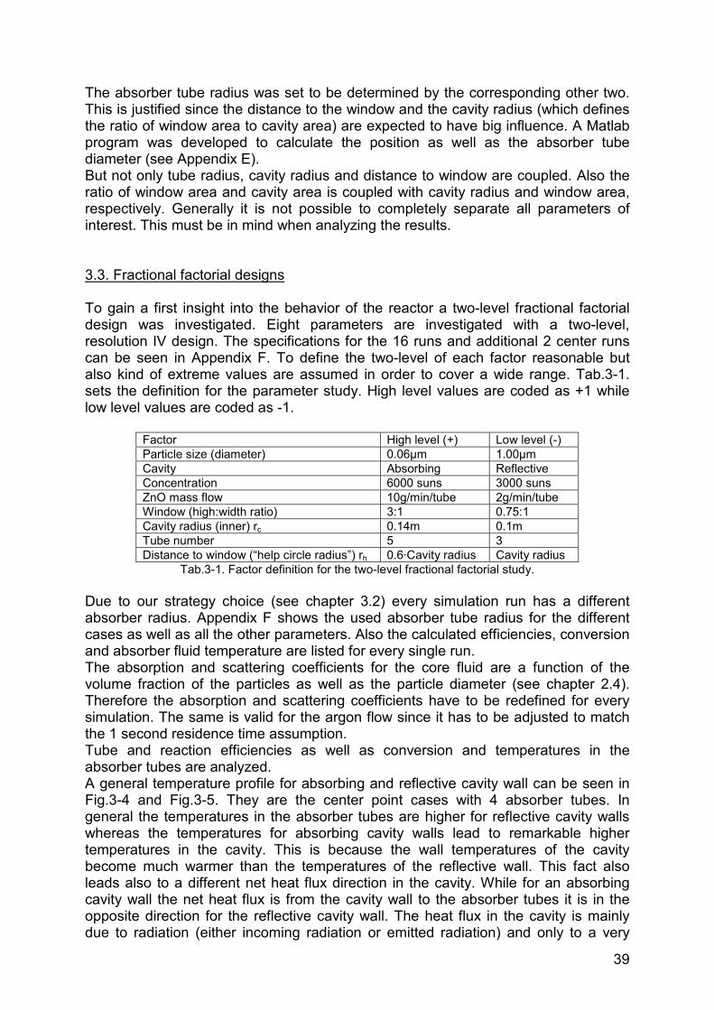
39

The absorber tube radius was set to be determined by the corresponding other two. This is justified since the distance to the window and the cavity radius (which defines the ratio of window area to cavity area) are expected to have big influence. A Matlab program was developed to calculate the position as well as the absorber tube diameter (see Appendix E). But not only tube radius, cavity radius and distance to window are coupled. Also the ratio of window area and cavity area is coupled with cavity radius and window area, respectively. Generally it is not possible to completely separate all parameters of interest. This must be in mind when analyzing the results.

3.3. Fractional factorial designs

To gain a first insight into the behavior of the reactor a two-level fractional factorial design was investigated. Eight parameters are investigated with a two-level, resolution IV design. The specifications for the 16 runs and additional 2 center runs can be seen in Appendix F. To define the two-level of each factor reasonable but also kind of extreme values are assumed in order to cover a wide range. Tab.3-1. sets the definition for the parameter study. High level values are coded as +1 while low level values are coded as -1.

Factor High level (+) Low level (-) Particle size (diameter) 0.06µm 1.00µm Cavity Absorbing Reflective Concentration 6000 suns 3000 suns ZnO mass flow 10g/min/tube 2g/min/tube Window (high:width ratio) 3:1 0.75:1 Cavity radius (inner) rc 0.14m 0.1m Tube number 5 3 Distance to window (“help circle radius”) rh 0.6·Cavity radius Cavity radius

Tab.3-1. Factor definition for the two-level fractional factorial study. Due to our strategy choice (see chapter 3.2) every simulation run has a different absorber radius. Appendix F shows the used absorber tube radius for the different cases as well as all the other parameters. Also the calculated efficiencies, conversion and absorber fluid temperature are listed for every single run. The absorption and scattering coefficients for the core fluid are a function of the volume fraction of the particles as well as the particle diameter (see chapter 2.4). Therefore the absorption and scattering coefficients have to be redefined for every simulation. The same is valid for the argon flow since it has to be adjusted to match the 1 second residence time assumption. Tube and reaction efficiencies as well as conversion and temperatures in the absorber tubes are analyzed. A general temperature profile for absorbing and reflective cavity wall can be seen in Fig.3-4 and Fig.3-5. They are the center point cases with 4 absorber tubes. In general the temperatures in the absorber tubes are higher for reflective cavity walls whereas the temperatures for absorbing cavity walls lead to remarkable higher temperatures in the cavity. This is because the wall temperatures of the cavity become much warmer than the temperatures of the reflective wall. This fact also leads also to a different net heat flux direction in the cavity. While for an absorbing cavity wall the net heat flux is from the cavity wall to the absorber tubes it is in the opposite direction for the reflective cavity wall. The heat flux in the cavity is mainly due to radiation (either incoming radiation or emitted radiation) and only to a very

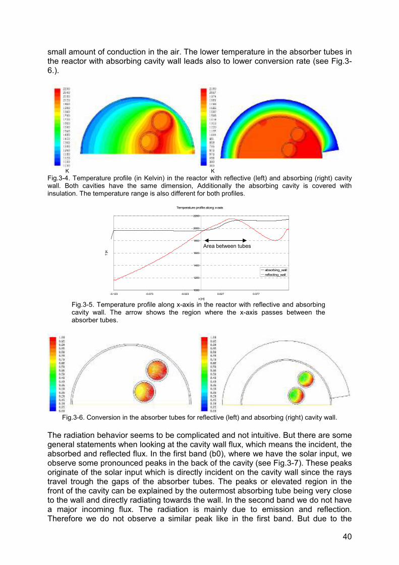
40

small amount of conduction in the air. The lower temperature in the absorber tubes in the reactor with absorbing cavity wall leads also to lower conversion rate (see Fig.3-6.).

K KFig.3-4. Temperature profile (in Kelvin) in the reactor with reflective (left) and absorbing (right) cavity wall. Both cavities have the same dimension, Additionally the absorbing cavity is covered with insulation. The temperature range is also different for both profiles.

Temperature profile along x-axis

1000

1200

1400

1600

1800

2000

2200

-0.123 -0.073 -0.023 0.027 0.077

x [m]

T[K

absorbing_wallreflecting_wall

Fig.3-5. Temperature profile along x-axis in the reactor with reflective and absorbing cavity wall. The arrow shows the region where the x-axis passes between the absorber tubes.

Fig.3-6. Conversion in the absorber tubes for reflective (left) and absorbing (right) cavity wall. The radiation behavior seems to be complicated and not intuitive. But there are some general statements when looking at the cavity wall flux, which means the incident, the absorbed and reflected flux. In the first band (b0), where we have the solar input, we observe some pronounced peaks in the back of the cavity (see Fig.3-7). These peaks originate of the solar input which is directly incident on the cavity wall since the rays travel trough the gaps of the absorber tubes. The peaks or elevated region in the front of the cavity can be explained by the outermost absorbing tube being very close to the wall and directly radiating towards the wall. In the second band we do not have a major incoming flux. The radiation is mainly due to emission and reflection. Therefore we do not observe a similar peak like in the first band. But due to the

Area between tubes

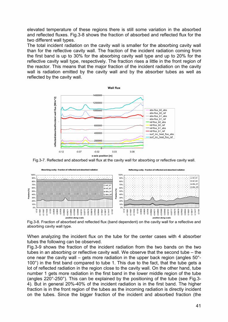
41

elevated temperature of these regions there is still some variation in the absorbed and reflected fluxes. Fig.3-8 shows the fraction of absorbed and reflected flux for the two different wall types. The total incident radiation on the cavity wall is smaller for the absorbing cavity wall than for the reflective cavity wall. The fraction of the incident radiation coming from the first band is up to 30% for the absorbing cavity wall type and up to 20% for the reflective cavity wall type, respectively. The fraction rises a little in the front region of the reactor. This means that the major fraction of the incident radiation on the cavity wall is radiation emitted by the cavity wall and by the absorber tubes as well as reflected by the cavity wall.

Wall flux

0

200000

400000

600000

800000

1000000

1200000

1400000

-0.12 -0.07 -0.02 0.03 0.08

x-axis position [m]

refle

cted

/abs

orbe

d/In

cide

ntw

allf

lux

[W/m

^2]

.

abs-flux_b0_absabs-flux_b0_refabs-flux_b1_absabs-flux_b1_refref-flux_b0_absref-flux_b0_refref-flux_b1_absref-flux_b1_refsurf_inc_heat_flux_abssurf_inc_heat_flux_ref

Fig.3-7. Reflected and absorbed wall flux at the cavity wall for absorbing or reflective cavity wall.

Absorbing cavity - fraction of reflected and absorbed radiation

0%

10%

20%

30%

40%

50%

60%

70%

80%

90%

100%

-0.1

2

-0.1

1891

-0.1

1567

-0.1

1034

-0.1

03

-0.0

938

-0.0

829

-0.0

705

-0.0

5682

-0.0

4211

-0.0

2664

-0.0

1069

0.00

546

0.02

151

0.03

717

0.05

215

0.06

619

0.07

903

0.09

044

0.10

021

0.10

817

0.11

417

0.11

81

position along x-axis

Frac

tion

[%]

ref_b1

ref_b0

abs_b1

abs_b0

Reflecting cavity - fraction of reflected and absorbed radiation

0%

10%

20%

30%

40%

50%

60%

70%

80%

90%

100%

-0.1

2

-0.1

1891

-0.1

1567

-0.1

1034

-0.1

03

-0.0

938

-0.0

829

-0.0

705

-0.0

5682

-0.0

4211

-0.0

2664

-0.0

1069

0.00

546

0.02

151

0.03

717

0.05

215

0.06

619

0.07

903

0.09

044

0.10

021

0.10

817

0.11

417

0.11

81

position along x-axis

Frac

tion

[%]

ref_b1

ref_b0

abs_b1

abs_b0

Fig.3-8. Fraction of absorbed and reflected flux (band dependent) on the cavity wall for a reflective and absorbing cavity wall type. When analyzing the incident flux on the tube for the center cases with 4 absorber tubes the following can be observed. Fig.3-9 shows the fraction of the incident radiation from the two bands on the two tubes in an absorbing or reflective cavity wall. We observe that the second tube – the one near the cavity wall – gets more radiation in the upper back region (angles 50°-100°) in the first band compared to tube 1. This due to the fact, that the tube gets a lot of reflected radiation in the region close to the cavity wall. On the other hand, tube number 1 gets more radiation in the first band in the lower middle region of the tube (angles 220°-250°). This can be explained by the positioning of the tube (see Fig.3-4). But in general 20%-40% of the incident radiation is in the first band. The higher fraction is in the front region of the tubes as the incoming radiation is directly incident on the tubes. Since the bigger fraction of the incident and absorbed fraction (the

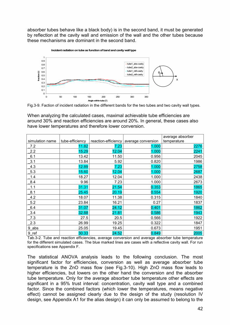
42

absorber tubes behave like a black body) is in the second band, it must be generated by reflection at the cavity wall and emission of the wall and the other tubes because these mechanisms are dominant in the second band.

Incident radiation on tube as function of band and cavity wall type

00.1

0.20.3

0.40.50.6

0.70.8

0.91

0 50 100 150 200 250 300 350

Angle within tube [°]

frac

tion

[-]

tube1_abs-cavitytube2_abs-cavitytube1_refl-cavitytube2_refl-cavity

Fig.3-9. Faction of incident radiation in the different bands for the two tubes and two cavity wall types. When analyzing the calculated cases, maximal achievable tube efficiencies are around 30% and reaction efficiencies are around 20%. In general, these cases also have lower temperatures and therefore lower conversion.

simulation name tube-efficiency reaction-efficiency average conversion average absorber temperature

_7.2 11.82 7.23 1.000 2276_2.2 15.29 12.04 1.000 2241_6.1 13.42 11.50 0.956 2045_3.1 13.84 5.92 0.820 1986_4.3 12.89 7.23 1.000 2758_5.3 15.60 12.04 1.000 2687_1.4 18.27 12.04 1.000 2438_8.4 9.96 7.23 1.000 2673_1.1 31.31 21.54 0.353 1865_8.1 25.45 20.19 0.554 1920_4.2 18.07 11.38 0.315 1840_5.2 23.84 16.21 0.27 1837_6.4 31.07 24.12 0.401 1862_3.4 32.88 21.81 0.586 1943_7.3 27.5 20.5 0.566 1922_2.3 26.99 19.25 0.322 18479_abs 25.05 19.45 0.673 19519_ref 30.33 24.52 0.849 2005Tab.3-2. Tube and reaction efficiencies, average conversion and average absorber tube temperature for the different simulated cases. The blue marked lines are cases with a reflective cavity wall. For run specifications see Appendix F. The statistical ANOVA analysis leads to the following conclusion. The most significant factor for efficiencies, conversion as well as average absorber tube temperature is the ZnO mass flow (see Fig.3-10). High ZnO mass flow leads to higher efficiencies, but lowers on the other hand the conversion and the absorber tube temperature. Only for the average absorber tube temperature other effects are significant in a 95% trust interval: concentration, cavity wall type and a combined factor. Since the combined factors (which lower the temperatures, means negative effect) cannot be assigned clearly due to the design of the study (resolution IV design, see Appendix A1 for the alias design) it can only be assumed to belong to the

x

θ

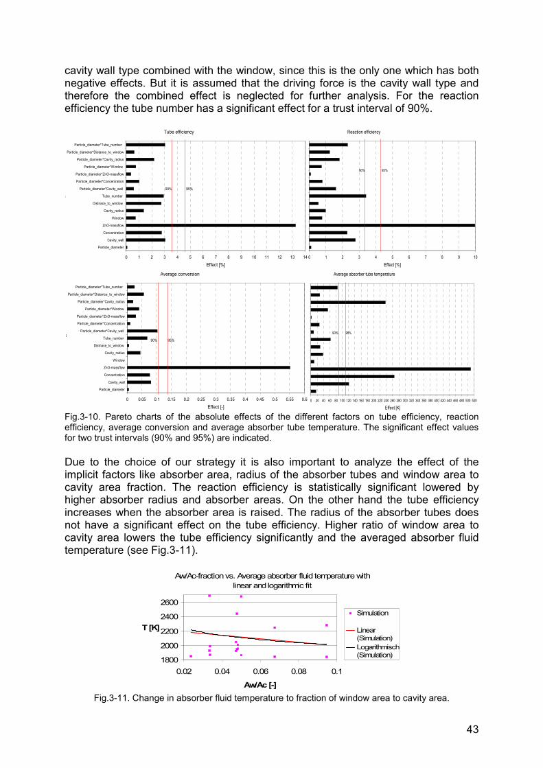
43

cavity wall type combined with the window, since this is the only one which has both negative effects. But it is assumed that the driving force is the cavity wall type and therefore the combined effect is neglected for further analysis. For the reaction efficiency the tube number has a significant effect for a trust interval of 90%.

Tube efficiency

0 1 2 3 4 5 6 7 8 9 10 11 12 13 14

Particle_diameter

Cavity_wall

Concentration

ZnO-massflow

Window

Cavity_radius

Distnace_to_window

Tube_number

Particle_diameter*Cavity_wall

Particle_diameter*Concentration

Particle_diameter*ZnO-massflow

Particle_diameter*Window

Particle_diameter*Cavity_radius

Particle_diameter*Distance_to_window

Particle_diameter*Tube_number

s

Effect [%]

90% 95%

Reaction efficiency

0 1 2 3 4 5 6 7 8 9 10

Effect [%]

90% 95%

Average conversion

0 0.05 0.1 0.15 0.2 0.25 0.3 0.35 0.4 0.45 0.5 0.55 0.6

Particle_diameter

Cavity_wall

Concentration

ZnO-massflow

Window

Cavity_radius

Distnace_to_window

Tube_number

Particle_diameter*Cavity_wall

Particle_diameter*Concentration

Particle_diameter*ZnO-massflow

Particle_diameter*Window

Particle_diameter*Cavity_radius

Particle_diameter*Distance_to_window

Particle_diameter*Tube_number

s

Effect [-]

90% 95%

Average absorber tube temperature

0 20 40 60 80 100 120 140 160 180 200 220 240 260 280 300 320 340 360 380 400 420 440 460 480 500 520

Effect [K]

90% 95%

Fig.3-10. Pareto charts of the absolute effects of the different factors on tube efficiency, reaction efficiency, average conversion and average absorber tube temperature. The significant effect values for two trust intervals (90% and 95%) are indicated. Due to the choice of our strategy it is also important to analyze the effect of the implicit factors like absorber area, radius of the absorber tubes and window area to cavity area fraction. The reaction efficiency is statistically significant lowered by higher absorber radius and absorber areas. On the other hand the tube efficiency increases when the absorber area is raised. The radius of the absorber tubes does not have a significant effect on the tube efficiency. Higher ratio of window area to cavity area lowers the tube efficiency significantly and the averaged absorber fluid temperature (see Fig.3-11).

Aw/Ac-fraction vs. Average absorber fluid temperature with linear and logarithmic fit

1800

2000

2200

2400

2600

0.02 0.04 0.06 0.08 0.1

Aw/Ac [-]

T [K]

Simulation

Linear(Simulation)Logarithmisch(Simulation)

Fig.3-11. Change in absorber fluid temperature to fraction of window area to cavity area.

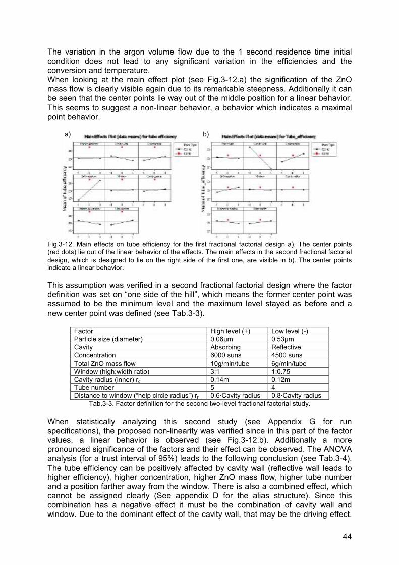
44

The variation in the argon volume flow due to the 1 second residence time initial condition does not lead to any significant variation in the efficiencies and the conversion and temperature. When looking at the main effect plot (see Fig.3-12.a) the signification of the ZnO mass flow is clearly visible again due to its remarkable steepness. Additionally it can be seen that the center points lie way out of the middle position for a linear behavior. This seems to suggest a non-linear behavior, a behavior which indicates a maximal point behavior.

Fig.3-12. Main effects on tube efficiency for the first fractional factorial design a). The center points (red dots) lie out of the linear behavior of the effects. The main effects in the second fractional factorial design, which is designed to lie on the right side of the first one, are visible in b). The center points indicate a linear behavior. This assumption was verified in a second fractional factorial design where the factor definition was set on “one side of the hill”, which means the former center point was assumed to be the minimum level and the maximum level stayed as before and a new center point was defined (see Tab.3-3).

Factor High level (+) Low level (-) Particle size (diameter) 0.06µm 0.53µm Cavity Absorbing Reflective Concentration 6000 suns 4500 suns Total ZnO mass flow 10g/min/tube 6g/min/tube Window (high:width ratio) 3:1 1:0.75 Cavity radius (inner) rc 0.14m 0.12m Tube number 5 4 Distance to window (“help circle radius”) rh 0.6·Cavity radius 0.8·Cavity radius

Tab.3-3. Factor definition for the second two-level fractional factorial study. When statistically analyzing this second study (see Appendix G for run specifications), the proposed non-linearity was verified since in this part of the factor values, a linear behavior is observed (see Fig.3-12.b). Additionally a more pronounced significance of the factors and their effect can be observed. The ANOVA analysis (for a trust interval of 95%) leads to the following conclusion (see Tab.3-4). The tube efficiency can be positively affected by cavity wall (reflective wall leads to higher efficiency), higher concentration, higher ZnO mass flow, higher tube number and a position farther away from the window. There is also a combined effect, which cannot be assigned clearly (See appendix D for the alias structure). Since this combination has a negative effect it must be the combination of cavity wall and window. Due to the dominant effect of the cavity wall, that may be the driving effect.

a) b)

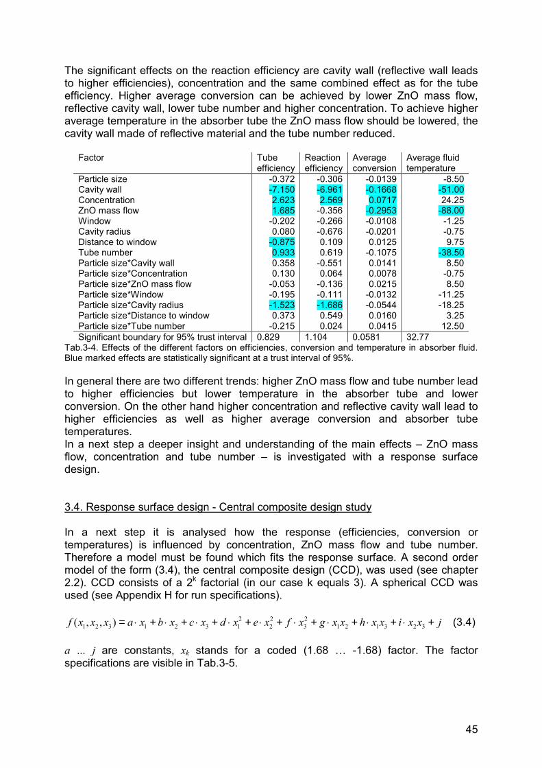
45

The significant effects on the reaction efficiency are cavity wall (reflective wall leads to higher efficiencies), concentration and the same combined effect as for the tube efficiency. Higher average conversion can be achieved by lower ZnO mass flow, reflective cavity wall, lower tube number and higher concentration. To achieve higher average temperature in the absorber tube the ZnO mass flow should be lowered, the cavity wall made of reflective material and the tube number reduced.

Factor Tube efficiency

Reaction efficiency

Average conversion

Average fluid temperature

Particle size Cavity wall Concentration ZnO mass flow Window Cavity radius Distance to window Tube number Particle size*Cavity wall Particle size*Concentration Particle size*ZnO mass flow Particle size*Window Particle size*Cavity radius Particle size*Distance to window Particle size*Tube number

-0.372 -7.1502.6231.685

-0.202 0.080

-0.8750.9330.358 0.130

-0.053 -0.195 -1.5230.373

-0.215

-0.306 -6.9612.569

-0.356 -0.266 -0.676 0.109 0.619

-0.551 0.064

-0.136 -0.111 -1.6860.549 0.024

-0.0139 -0.16680.0717

-0.2953-0.0108 -0.0201 0.0125

-0.10750.0141 0.0078 0.0215

-0.0132 -0.0544 0.0160 0.0415

-8.50 -51.00 24.25

-88.00-1.25 -0.75 9.75

-38.508.50

-0.75 8.50

-11.25 -18.25

3.25 12.50

Significant boundary for 95% trust interval 0.829 1.104 0.0581 32.77 Tab.3-4. Effects of the different factors on efficiencies, conversion and temperature in absorber fluid. Blue marked effects are statistically significant at a trust interval of 95%. In general there are two different trends: higher ZnO mass flow and tube number lead to higher efficiencies but lower temperature in the absorber tube and lower conversion. On the other hand higher concentration and reflective cavity wall lead to higher efficiencies as well as higher average conversion and absorber tube temperatures. In a next step a deeper insight and understanding of the main effects – ZnO mass flow, concentration and tube number – is investigated with a response surface design.

3.4. Response surface design - Central composite design study

In a next step it is analysed how the response (efficiencies, conversion or temperatures) is influenced by concentration, ZnO mass flow and tube number. Therefore a model must be found which fits the response surface. A second order model of the form (3.4), the central composite design (CCD), was used (see chapter 2.2). CCD consists of a 2k factorial (in our case k equals 3). A spherical CCD was used (see Appendix H for run specifications).

jxxixxhxxgxfxexdxcxbxaxxxf +⋅+⋅+⋅+⋅+⋅+⋅+⋅+⋅+⋅= 32312123

22

21321321 ),,( (3.4)

a … j are constants, xk stands for a coded (1.68 … -1.68) factor. The factor specifications are visible in Tab.3-5.

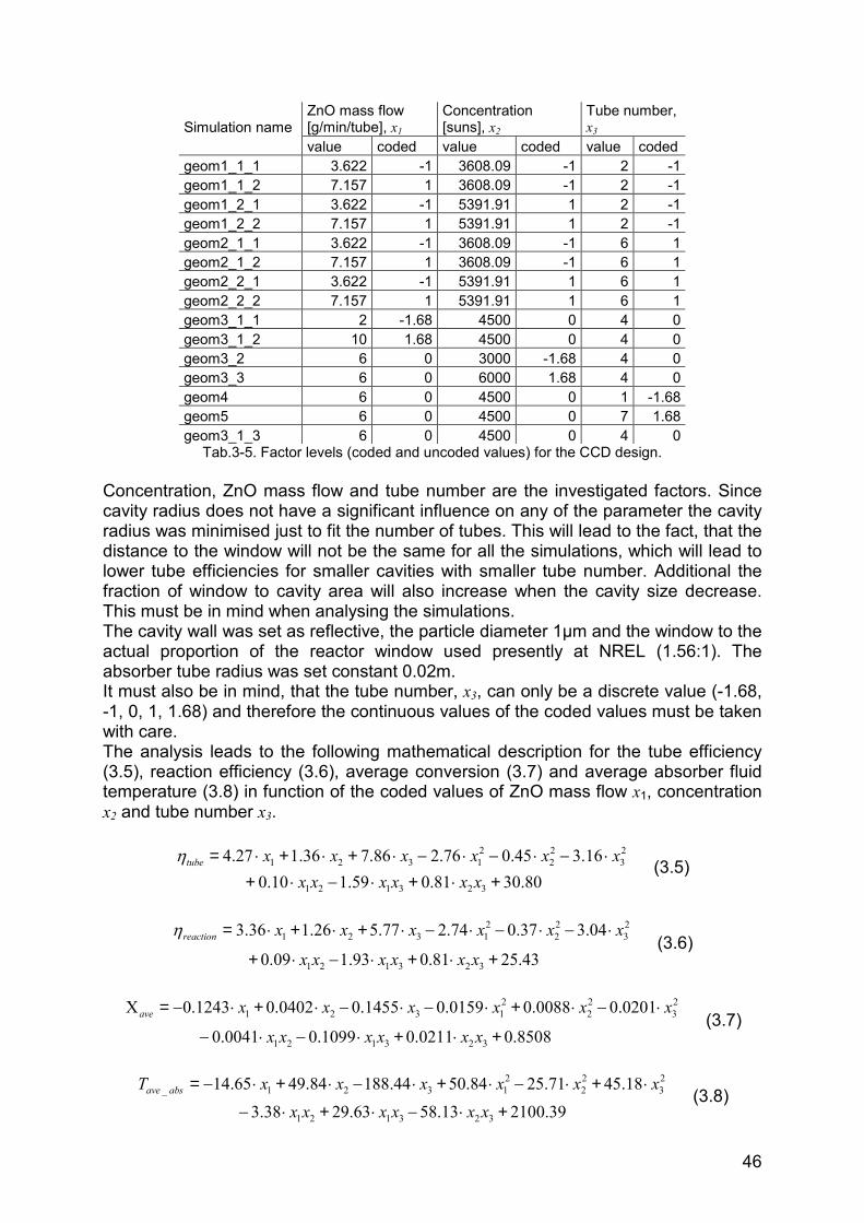
46

Simulation name ZnO mass flow [g/min/tube], x1

Concentration [suns], x2

Tube number, x3

value coded value coded value codedgeom1_1_1 3.622 -1 3608.09 -1 2 -1geom1_1_2 7.157 1 3608.09 -1 2 -1geom1_2_1 3.622 -1 5391.91 1 2 -1geom1_2_2 7.157 1 5391.91 1 2 -1geom2_1_1 3.622 -1 3608.09 -1 6 1geom2_1_2 7.157 1 3608.09 -1 6 1geom2_2_1 3.622 -1 5391.91 1 6 1geom2_2_2 7.157 1 5391.91 1 6 1geom3_1_1 2 -1.68 4500 0 4 0geom3_1_2 10 1.68 4500 0 4 0geom3_2 6 0 3000 -1.68 4 0geom3_3 6 0 6000 1.68 4 0geom4 6 0 4500 0 1 -1.68geom5 6 0 4500 0 7 1.68geom3_1_3 6 0 4500 0 4 0

Tab.3-5. Factor levels (coded and uncoded values) for the CCD design. Concentration, ZnO mass flow and tube number are the investigated factors. Since cavity radius does not have a significant influence on any of the parameter the cavity radius was minimised just to fit the number of tubes. This will lead to the fact, that the distance to the window will not be the same for all the simulations, which will lead to lower tube efficiencies for smaller cavities with smaller tube number. Additional the fraction of window to cavity area will also increase when the cavity size decrease. This must be in mind when analysing the simulations. The cavity wall was set as reflective, the particle diameter 1µm and the window to the actual proportion of the reactor window used presently at NREL (1.56:1). The absorber tube radius was set constant 0.02m. It must also be in mind, that the tube number, x3, can only be a discrete value (-1.68, -1, 0, 1, 1.68) and therefore the continuous values of the coded values must be taken with care. The analysis leads to the following mathematical description for the tube efficiency (3.5), reaction efficiency (3.6), average conversion (3.7) and average absorber fluid temperature (3.8) in function of the coded values of ZnO mass flow x1, concentration x2 and tube number x3.

80.3081.059.110.016.345.076.286.736.127.4

323121

23

22

21321

+⋅+⋅−⋅+⋅−⋅−⋅−⋅+⋅+⋅=

xxxxxxxxxxxxtubeη

(3.5)

43.2581.093.109.0

04.337.074.277.526.136.3

323121

23

22

21321

+⋅+⋅−⋅+

⋅−⋅−⋅−⋅+⋅+⋅=

xxxxxx

xxxxxxreactionη(3.6)

8508.00211.01099.00041.0

0201.00088.00159.01455.00402.01243.0

323121

23

22

21321

+⋅+⋅−⋅−

⋅−⋅+⋅−⋅−⋅+⋅−=Χ

xxxxxx

xxxxxxave (3.7)

39.210013.5863.2938.3

18.4571.2584.5044.18884.4965.14

323121

23

22

21321_

+⋅−⋅+⋅−

⋅+⋅−⋅+⋅−⋅+⋅−=

xxxxxxxxxxxxT absave (3.8)

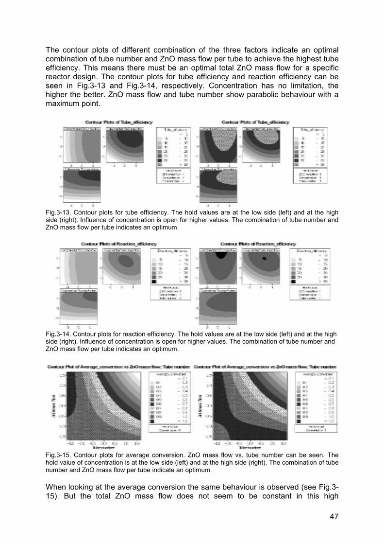
47

The contour plots of different combination of the three factors indicate an optimal combination of tube number and ZnO mass flow per tube to achieve the highest tube efficiency. This means there must be an optimal total ZnO mass flow for a specific reactor design. The contour plots for tube efficiency and reaction efficiency can be seen in Fig.3-13 and Fig.3-14, respectively. Concentration has no limitation, the higher the better. ZnO mass flow and tube number show parabolic behaviour with a maximum point.

Fig.3-13. Contour plots for tube efficiency. The hold values are at the low side (left) and at the high side (right). Influence of concentration is open for higher values. The combination of tube number and ZnO mass flow per tube indicates an optimum.

Fig.3-14. Contour plots for reaction efficiency. The hold values are at the low side (left) and at the high side (right). Influence of concentration is open for higher values. The combination of tube number and ZnO mass flow per tube indicates an optimum.

Fig.3-15. Contour plots for average conversion. ZnO mass flow vs. tube number can be seen. The hold value of concentration is at the low side (left) and at the high side (right). The combination of tube number and ZnO mass flow per tube indicate an optimum. When looking at the average conversion the same behaviour is observed (see Fig.3-15). But the total ZnO mass flow does not seem to be constant in this high

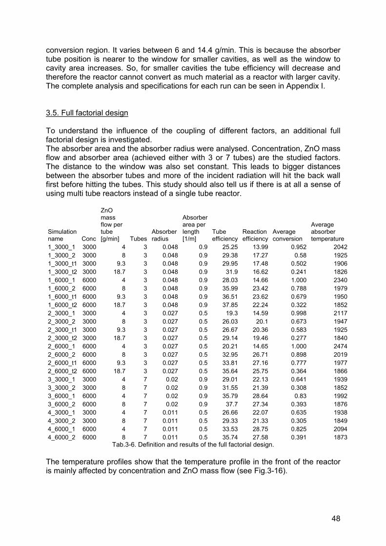
48

conversion region. It varies between 6 and 14.4 g/min. This is because the absorber tube position is nearer to the window for smaller cavities, as well as the window to cavity area increases. So, for smaller cavities the tube efficiency will decrease and therefore the reactor cannot convert as much material as a reactor with larger cavity. The complete analysis and specifications for each run can be seen in Appendix I.

3.5. Full factorial design

To understand the influence of the coupling of different factors, an additional full factorial design is investigated. The absorber area and the absorber radius were analysed. Concentration, ZnO mass flow and absorber area (achieved either with 3 or 7 tubes) are the studied factors. The distance to the window was also set constant. This leads to bigger distances between the absorber tubes and more of the incident radiation will hit the back wall first before hitting the tubes. This study should also tell us if there is at all a sense of using multi tube reactors instead of a single tube reactor.

Simulation name Conc

ZnO mass flow per tube [g/min] Tubes

Absorber radius

Absorber area per length [1/m]

Tube efficiency

Reaction efficiency

Average conversion

Average absorber temperature

1_3000_1 3000 4 3 0.048 0.9 25.25 13.99 0.952 20421_3000_2 3000 8 3 0.048 0.9 29.38 17.27 0.58 19251_3000_t1 3000 9.3 3 0.048 0.9 29.95 17.48 0.502 19061_3000_t2 3000 18.7 3 0.048 0.9 31.9 16.62 0.241 18261_6000_1 6000 4 3 0.048 0.9 28.03 14.66 1.000 23401_6000_2 6000 8 3 0.048 0.9 35.99 23.42 0.788 19791_6000_t1 6000 9.3 3 0.048 0.9 36.51 23.62 0.679 19501_6000_t2 6000 18.7 3 0.048 0.9 37.85 22.24 0.322 18522_3000_1 3000 4 3 0.027 0.5 19.3 14.59 0.998 21172_3000_2 3000 8 3 0.027 0.5 26.03 20.1 0.673 19472_3000_t1 3000 9.3 3 0.027 0.5 26.67 20.36 0.583 19252_3000_t2 3000 18.7 3 0.027 0.5 29.14 19.46 0.277 18402_6000_1 6000 4 3 0.027 0.5 20.21 14.65 1.000 24742_6000_2 6000 8 3 0.027 0.5 32.95 26.71 0.898 20192_6000_t1 6000 9.3 3 0.027 0.5 33.81 27.16 0.777 19772_6000_t2 6000 18.7 3 0.027 0.5 35.64 25.75 0.364 18663_3000_1 3000 4 7 0.02 0.9 29.01 22.13 0.641 19393_3000_2 3000 8 7 0.02 0.9 31.55 21.39 0.308 18523_6000_1 6000 4 7 0.02 0.9 35.79 28.64 0.83 19923_6000_2 6000 8 7 0.02 0.9 37.7 27.34 0.393 18764_3000_1 3000 4 7 0.011 0.5 26.66 22.07 0.635 19384_3000_2 3000 8 7 0.011 0.5 29.33 21.33 0.305 18494_6000_1 6000 4 7 0.011 0.5 33.53 28.75 0.825 20944_6000_2 6000 8 7 0.011 0.5 35.74 27.58 0.391 1873

Tab.3-6. Definition and results of the full factorial design. The temperature profiles show that the temperature profile in the front of the reactor is mainly affected by concentration and ZnO mass flow (see Fig.3-16).

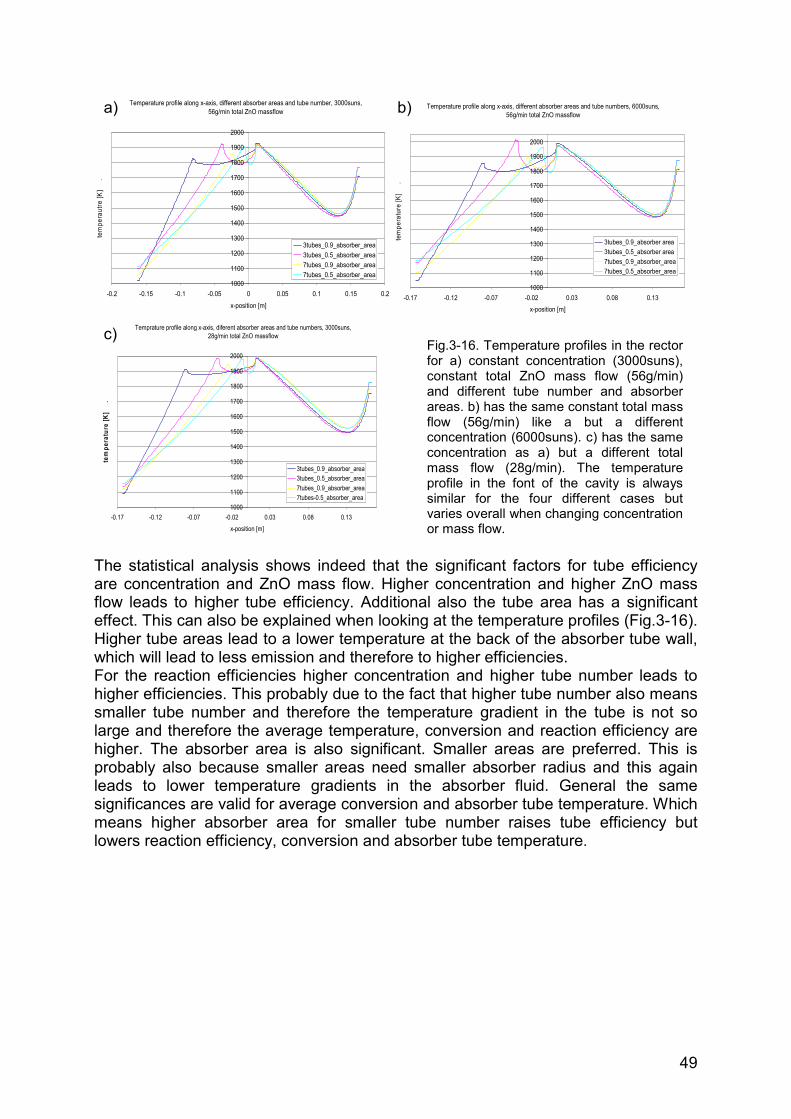
49

Temperature profile along x-axis, different absorber areas and tube number, 3000suns, 56g/min total ZnO massflow

1000

1100

1200

1300

1400

1500

1600

1700

1800

1900

2000

-0.2 -0.15 -0.1 -0.05 0 0.05 0.1 0.15 0.2

x-position [m]

tem

pera

utre

[K]

.

3tubes_0.9_absorber_area3tubes_0.5_absorber_area7tubes_0.9_absorber_area7tubes_0.5_absorber_area

Temperature profile along x-axis, different absorber areas and tube numbers, 6000suns, 56g/min total ZnO massflow

1000

1100

1200

1300

1400

1500

1600

1700

1800

1900

2000

-0.17 -0.12 -0.07 -0.02 0.03 0.08 0.13

x-position [m]

tem

pera

ture

[K]

.

3tubes_0.9_absorber area3tubes_0.5_absorber area7tubes_0.9_absorber_area7tubes_0.5_absorber_area

Temprature profile along x-axis, diferent absorber areas and tube numbers, 3000suns,

28g/min total ZnO massflow

1000

1100

1200

1300

1400

1500

1600

1700

1800

1900

2000

-0.17 -0.12 -0.07 -0.02 0.03 0.08 0.13

x-position [m]

tem

pera

ture

[K]

.

3tubes_0.9_absorber_area3tubes_0.5_absorber_area7tubes_0.9_absorber_area7tubes-0.5_absorber_area

The statistical analysis shows indeed that the significant factors for tube efficiency are concentration and ZnO mass flow. Higher concentration and higher ZnO mass flow leads to higher tube efficiency. Additional also the tube area has a significant effect. This can also be explained when looking at the temperature profiles (Fig.3-16). Higher tube areas lead to a lower temperature at the back of the absorber tube wall, which will lead to less emission and therefore to higher efficiencies. For the reaction efficiencies higher concentration and higher tube number leads to higher efficiencies. This probably due to the fact that higher tube number also means smaller tube number and therefore the temperature gradient in the tube is not so large and therefore the average temperature, conversion and reaction efficiency are higher. The absorber area is also significant. Smaller areas are preferred. This is probably also because smaller areas need smaller absorber radius and this again leads to lower temperature gradients in the absorber fluid. General the same significances are valid for average conversion and absorber tube temperature. Which means higher absorber area for smaller tube number raises tube efficiency but lowers reaction efficiency, conversion and absorber tube temperature.

Fig.3-16. Temperature profiles in the rector for a) constant concentration (3000suns), constant total ZnO mass flow (56g/min) and different tube number and absorber areas. b) has the same constant total mass flow (56g/min) like a but a different concentration (6000suns). c) has the same concentration as a) but a different total mass flow (28g/min). The temperature profile in the font of the cavity is always similar for the four different cases but varies overall when changing concentration or mass flow.

a) b)

c)

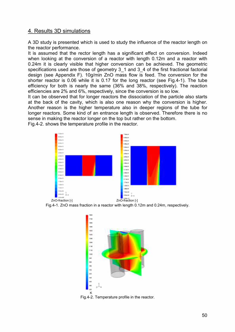
50

4. Results 3D simulations

A 3D study is presented which is used to study the influence of the reactor length on the reactor performance. It is assumed that the rector length has a significant effect on conversion. Indeed when looking at the conversion of a reactor with length 0.12m and a reactor with 0.24m it is clearly visible that higher conversion can be achieved. The geometric specifications used are those of geometry 3_1 and 3_4 of the first fractional factorial design (see Appendix F). 10g/min ZnO mass flow is feed. The conversion for the shorter reactor is 0.06 while it is 0.17 for the long reactor (see Fig.4-1). The tube efficiency for both is nearly the same (36% and 38%, respectively). The reaction efficiencies are 2% and 6%, respectively, since the conversion is so low. It can be observed that for longer reactors the dissociation of the particle also starts at the back of the cavity, which is also one reason why the conversion is higher. Another reason is the higher temperature also in deeper regions of the tube for longer reactors. Some kind of an entrance length is observed. Therefore there is no sense in making the reactor longer on the top but rather on the bottom. Fig.4-2. shows the temperature profile in the reactor.

Fig.4-1. ZnO mass fraction in a reactor with length 0.12m and 0.24m, respectively.

Fig.4-2. Temperature profile in the reactor.

ZnO-fraction [-] ZnO-fraction [-]

K

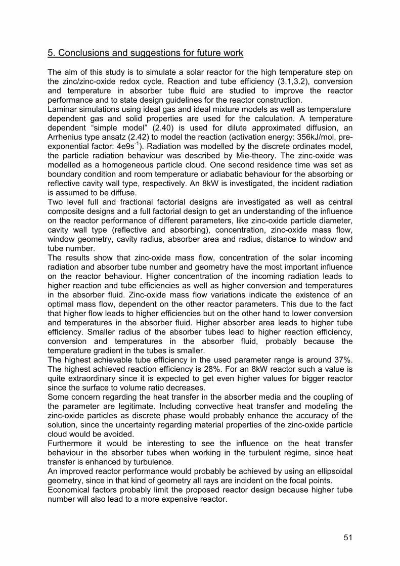
51

5. Conclusions and suggestions for future work

The aim of this study is to simulate a solar reactor for the high temperature step on the zinc/zinc-oxide redox cycle. Reaction and tube efficiency (3.1,3.2), conversion and temperature in absorber tube fluid are studied to improve the reactor performance and to state design guidelines for the reactor construction. Laminar simulations using ideal gas and ideal mixture models as well as temperature dependent gas and solid properties are used for the calculation. A temperature dependent “simple model” (2.40) is used for dilute approximated diffusion, an Arrhenius type ansatz (2.42) to model the reaction (activation energy: 356kJ/mol, pre-exponential factor: 4e9s-1). Radiation was modelled by the discrete ordinates model, the particle radiation behaviour was described by Mie-theory. The zinc-oxide was modelled as a homogeneous particle cloud. One second residence time was set as boundary condition and room temperature or adiabatic behaviour for the absorbing or reflective cavity wall type, respectively. An 8kW is investigated, the incident radiation is assumed to be diffuse. Two level full and fractional factorial designs are investigated as well as central composite designs and a full factorial design to get an understanding of the influence on the reactor performance of different parameters, like zinc-oxide particle diameter, cavity wall type (reflective and absorbing), concentration, zinc-oxide mass flow, window geometry, cavity radius, absorber area and radius, distance to window and tube number. The results show that zinc-oxide mass flow, concentration of the solar incoming radiation and absorber tube number and geometry have the most important influence on the reactor behaviour. Higher concentration of the incoming radiation leads to higher reaction and tube efficiencies as well as higher conversion and temperatures in the absorber fluid. Zinc-oxide mass flow variations indicate the existence of an optimal mass flow, dependent on the other reactor parameters. This due to the fact that higher flow leads to higher efficiencies but on the other hand to lower conversion and temperatures in the absorber fluid. Higher absorber area leads to higher tube efficiency. Smaller radius of the absorber tubes lead to higher reaction efficiency, conversion and temperatures in the absorber fluid, probably because the temperature gradient in the tubes is smaller. The highest achievable tube efficiency in the used parameter range is around 37%. The highest achieved reaction efficiency is 28%. For an 8kW reactor such a value is quite extraordinary since it is expected to get even higher values for bigger reactor since the surface to volume ratio decreases. Some concern regarding the heat transfer in the absorber media and the coupling of the parameter are legitimate. Including convective heat transfer and modeling the zinc-oxide particles as discrete phase would probably enhance the accuracy of the solution, since the uncertainty regarding material properties of the zinc-oxide particle cloud would be avoided. Furthermore it would be interesting to see the influence on the heat transfer behaviour in the absorber tubes when working in the turbulent regime, since heat transfer is enhanced by turbulence. An improved reactor performance would probably be achieved by using an ellipsoidal geometry, since in that kind of geometry all rays are incident on the focal points. Economical factors probably limit the proposed reactor design because higher tube number will also lead to a more expensive reactor.

52

6. Acknowledgement

I would like to thank my family for their support. I would like to thank Prof. Aldo Steinfeld, head of the institute of renewable energy carriers at the Swiss Federal Institute of Technology at Zurich, for giving me the opportunity to work for this project at the University of Colorado at Boulder. I would like to thank Prof. Alan Weimer, Professor at the Chemical and Biological Department of the University of Colorado at Boulder, for making this project possible. I would like to thank Dr. David Hirsch, Postdoctoral student at the University of Colorado at Boulder, for the interesting discussions, the support in Fluent and the excellent team work. I would like to thank Dr. Christopher Perkins, Postdoctoral student at the University of Colorado at Boulder, for the time he took whenever I had questions and for the helpful information regarding chemical reactions. Additional I would like to thank all the Graduate students, Doctoral students and Postdoctoral students and other associates from the Team Weimer for their help during my stay at CU. It was a great, interesting and instructive time!

53

7. References

[1]

[2]

[3]

[4]

[5]

[6]

[7]

[8]

[9]

[10]

[11]

[12]

[13] [14]

[15]

[16]

Intergovernmental Panel on Climate Change, IPCC Fourth Assessment Report, Climate Change 2007: The Physical Science Basis, Summary for Policymakers, http://ipcc-wg1.ucar.edu/wg1/docs/WG1AR4_SPM_Approved_05Feb.pdf, 2007 International energy agency IAEA, Energy Outlook 2004, http://www.iea.org/textbase/nppdf/free/2004/weo2004.pdf, 2004 C.E. Tyner, G.J. Kolb, M. Geyer and M. Romero, “Concentrating solar power in 2001”, www.solarpaces.org, SolarPACES 2001 B. Schaffer, A. Meier, D. Wuillemin, W. Hoffelner and A. Steinfeld, “Recycling of Hazardous Solid Waste Material Using High-Temperature Solar Process Heat. 2. Reactor Design and Experimentation”, Environ. Sci. Technol., vol. 37, pp. 165-170, 2003 V. Nikulshina, D. Hirsch, M. Mazzotti and A. Steinfeld, “CO2 capture from air and co-production of H2 via the Ca(OH)2–CaCO3 cycle using concentrated solar power – Thermodynamic analysis”, Energy, vol. 31, pp. 1715–1725, 2006 M. Tsuji, Y. Wada, Y. Tamaura, A. Steinfeld, P. Kuhn and R. Palumbo, “Coal Gasification Using the ZnO/Zn Redox System”, Energy & Fuels, vol. 10, pp. 225-228, 1996 Y.Tamaura, Y. Wada, T. Yoshida, M.Tsuji, K. Ehrenberger and A. Steinfeld, “The Coal/Fe304 System for Mixing of Solar and Fossil Energies”, Energy, vol. 22, pp. 337-342, 1997 D. Trommer, F. Noembrini, M. Fasciana, D. Rodriguez, A. Moralesb, M. Romero and A. Steinfeld, “Hydrogen production by steam-gasification of petroleum coke using concentrated solar power—I. Thermodynamic and kinetic analyses”, International Journal of Hydrogen Energy, vol. 30, pp. 605-618, 2005 J.K. Dahl, A.W. Weimer, A. Lewandowski, C. Bingham, F. Bruetsch and Aldo Steinfeld, “Dry Reforming of Methane Using a Solar-Thermal Aerosol Flow Reactor”, Ind. Eng. Chem. Res., vol. 43, pp. 5489-5495,2004 J.K. Dahl, K.J. Buechler, R. Finley, T. Stanislaus, A.W. Weimer, A. Lewandowski, C. Bingham, A. Smeets and A. Schneider, “Rapid solar-thermal dissociation of natural gas in an aerosol flow reactor”, Energy, vol. 29, pp. 715–725, 2004 J.K. Dahl, K.J. Buechler, A.W. Weimer, A. Lewandowski and C. Bingham, “Solar-thermal dissociation of methane in a fuid-wall aerosol fow reactor”, International Journal of Hydrogen Energy, vol. 29, pp. 725 – 736, 2004 A. Meier, E. Bonaldi, G.M. Cella, W. Lipinski, D. Wuillemin and R. Palumbo, “Design and experimental investigation of a horizontal rotary reactor for the solar thermal production of lime”, Energy, vol. 29, pp. 811–821, 2004 T. Nakamura, “Hydrogen Production from Water Utilizing Solar Heat at High Temperatures”, Solar Energy, voI. 19, pp. 467-475, 1977 C. Perkins, “Solar thermal decomposition of ZnO in aerosol flow to facilitate renewable production of hydrogen”, Dissertation, University of Colorado, USA, 2006 S. Haussener, “Computational Fluid Dynamics modeling of an aerosol-flow reactor for the formation of Zn-nanoparticles followed by their in-situ hydrolysis for H2 generation”, Semester Thesis, ETHZ, Switzerland, 2006 A. Steinfeld and I. Spiewak, “Economic evaluation of the solar therma co-

54

[17]

[18]

[19]

[20]

[21]

[22]

[23] [24] [25] [26] [27] [28]

[29] [30] [31]

[32]

[33]

[34] [35]

production of zinc and synthesis gas”, Energy Convers. Mgmt, vol. 39, no. 15, pp. 1513-1518, 1998 C. Wieckert, R. Palumbo and U. Frommherz, “A two-cavity reactor for solar chemical processes: heat transfer model and application to carbothermic reduction of ZnO”, Energy, vol. 29, pp. 771–787, 2004 A. Steinfeld, M. Brack, A. Meier, A. Weidenkaff and D. Wuillemin, ”Solar chemical reactor for co-production of zinc and synthesis gas”, Energy, vol. 23, no. 10, pp. 803–814, 1998 P. Haueter, S. Moeller, R. Palumbo and A. Steinfeld, “The Production of Zinc by Thermal Dissociation of Zinc, Oxide—Solar Chemical Reactor Design”, Solar Energy, vol. 67, nos. 1–3, pp. 161–167, 1999 C. Wieckert, “Design Studies for a Solar Reactor Based on a Simple Radiative Heat Exchange Model”, Jou. Of Solar Energy Engineering, vol. 127, pp. 425-429, 2005 C. Agrafiotis, M. Roeb, A.G. Konstandopoulos, L. Nalbandian, V.T. Zaspalis, C. Sattler, P. Stobbe and A.M. Steele, “Solar water splitting for hydrogen production with monolithic reactors”, Solar Energy, vol. 79, pp. 409–421, 2005 M. Roeb, C. Sattler, R. Klüser, N. Monnerie, L. de Oliveira, A.G. Konstandopoulos, C. Agrafiotis, V.T. Zaspalis, L. Nalbandian, A. Steele and P. Stobbe, “Solar Hydrogen Production by a Two-Step Cycle Based on Mixed Iron Oxides”, Journal of Solar Energy Engineering, vol. 128, pp. 125-133, 2006 D.C. Montgomery, “Design and analysis of experiments”, John Wiley & sons, 6th Edition, USA: Arizona, 2005 R. Siegel and J.R. Howell, “Thermal Radiation Heat Transfer”, Hemisphere Publishing Corporation, 3rd Edition, USA, 1992 Fluent Reference Manual 6.3.21 beta: Fluent, Inc., 2006. C.F. Bohren and D.R. Huffmann, “Absorption and Scattering of Light by Small Particles”, John Wiley and Sons Inc., USA: New York, 1983 V. Srikant and D.R. Clarke, "On the Optical Band Gap of Zinc Oxide," J. Appl. Physics, vol. 83, pp. 5447-5451, 1998 S.M. Al-Hilli and M. Willander, "Optical Properties of Zinc Oxide Nano-Particles Embedded in Dielectric Medium for UV Region: Numerical Simulation," J. Nanoparticle Research, vol. 8, pp. 79-97, 2006 E.L. Cussler, Diffusion, Minnesota, USA: Cambridge University Press, 1984 VDI-Wärmeatlas, Düsseldorf, Germany: VDI-Verlag GmbH, 4.Auflage, 1984 A. Finch, P.J. Gardner, E. Tarbox and S. Yardley, “Binary Gaseous Diffusion Coefficients of Zinc in Hydrogen, Helium and Argon at 1 Atmosphere and 720-1120 K”, Journal of Chemical Society, vol. 3, pp. 545-549, 1979 P.J. Gardner, P. Pang and S.R. Preston, “Binary Gaseous Diffusion Coefficients of Mercury and of Zinc in Hydrogen, Helium, Argon, Nitrogen, and Carbon Dioxide“, Journal of Chemical and Engineering data, vol.36, pp. 265-268, 1991 B.V. L’vov, “Interpretation of atomization mechanisms in electrothermal atomic absorption spectrometry by analysis of the absolute rates of the processes”, Spectrochimica Acta Part B, vol. 52, pp. 1-23, 1997 O. Levenspiel, “Chemical Reaction Engineering”, John Wiley and Sons Inc., 3rd edition, USA: Oregon, 1999 American Inst. of Chem. Engineers, Design Inst. for Physical Properties, DIPPR® Project 801–Full Version, Evaluated Standard Thermophysical

55

[36] [37]

[38] [39]

Property Values, 2005 Public Release, BYU–DIPPR® Thermophysical Properties Laboratory, Brigham Young University, Provo, UT. C.L. Yaws, Chemical properties handbook, Texas, USA: McGraw-Hill Handbooks, 1999 S. Moller and R. Palumbo, “The development of a solar chemical reactor for the direct thermal dissociation of zinc oxide”, Journal of Solar Energy Engineering-Transactions of the ASME, vol. 123, no.2, pp. 83-90, 2001 T. Melchior, “Tubular Absorber surrounded by windowed tubular Cavity”, Diploma Thesis, ETHZ, Switzerland, 2005 D.A. Jaworske, “Reflectivity of Silver and Silver-Coated Substrates from 25°C to 800°C”, prepared for the 32nd IECEC, vol. 1, pp. 407-411, Honolulu, Hawaii, July, 1997

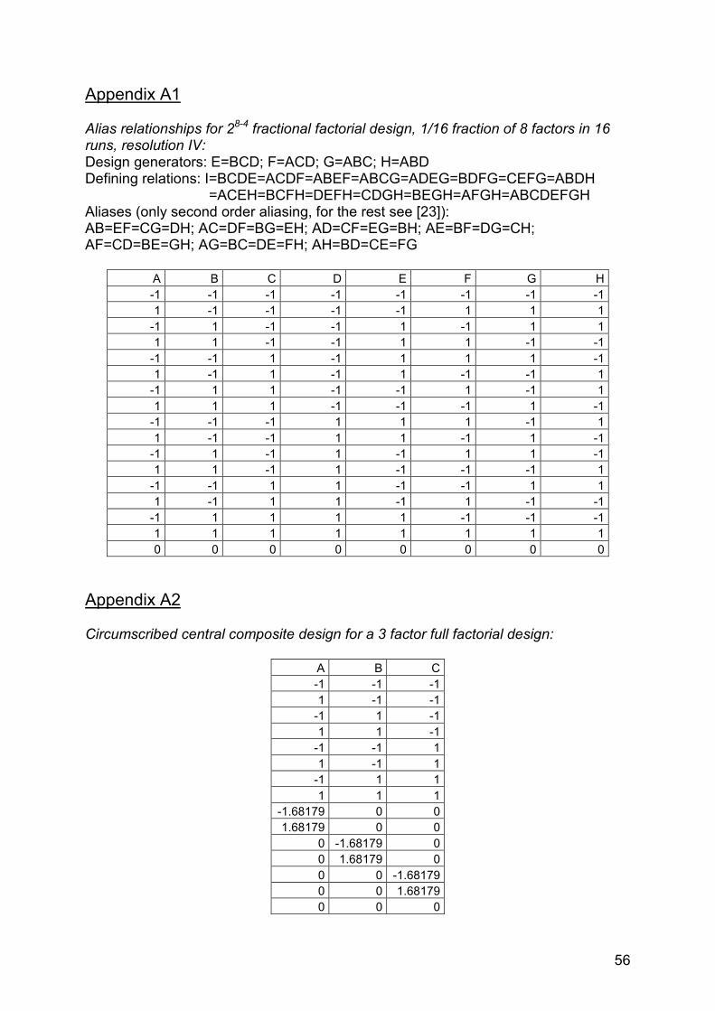
56

Appendix A1

Alias relationships for 28-4 fractional factorial design, 1/16 fraction of 8 factors in 16 runs, resolution IV: Design generators: E=BCD; F=ACD; G=ABC; H=ABD Defining relations: I=BCDE=ACDF=ABEF=ABCG=ADEG=BDFG=CEFG=ABDH =ACEH=BCFH=DEFH=CDGH=BEGH=AFGH=ABCDEFGH Aliases (only second order aliasing, for the rest see [23]): AB=EF=CG=DH; AC=DF=BG=EH; AD=CF=EG=BH; AE=BF=DG=CH; AF=CD=BE=GH; AG=BC=DE=FH; AH=BD=CE=FG

A B C D E F G H-1 -1 -1 -1 -1 -1 -1 -11 -1 -1 -1 -1 1 1 1

-1 1 -1 -1 1 -1 1 11 1 -1 -1 1 1 -1 -1

-1 -1 1 -1 1 1 1 -11 -1 1 -1 1 -1 -1 1

-1 1 1 -1 -1 1 -1 11 1 1 -1 -1 -1 1 -1

-1 -1 -1 1 1 1 -1 11 -1 -1 1 1 -1 1 -1

-1 1 -1 1 -1 1 1 -11 1 -1 1 -1 -1 -1 1

-1 -1 1 1 -1 -1 1 11 -1 1 1 -1 1 -1 -1

-1 1 1 1 1 -1 -1 -11 1 1 1 1 1 1 10 0 0 0 0 0 0 0

Appendix A2

Circumscribed central composite design for a 3 factor full factorial design:

A B C-1 -1 -11 -1 -1

-1 1 -11 1 -1

-1 -1 11 -1 1

-1 1 11 1 1

-1.68179 0 01.68179 0 0

0 -1.68179 00 1.68179 00 0 -1.681790 0 1.681790 0 0

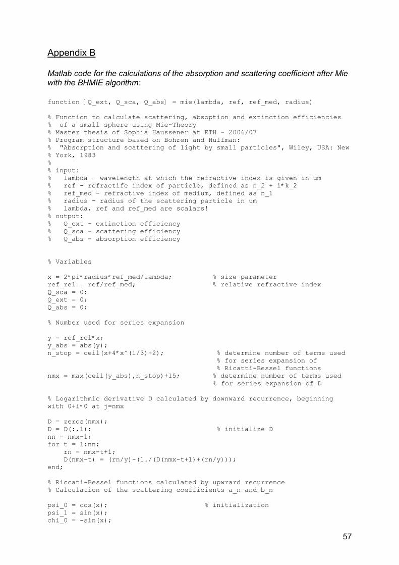
57

Appendix B

Matlab code for the calculations of the absorption and scattering coefficient after Mie with the BHMIE algorithm: function [Q_ext, Q_sca, Q_abs] = mie(lambda, ref, ref_med, radius) % Function to calculate scattering, absoption and extinction efficiencies % of a small sphere using Mie-Theory % Master thesis of Sophia Haussener at ETH - 2006/07 % Program structure based on Bohren and Huffman: % "Absorption and scattering of light by small particles", Wiley, USA: New % York, 1983 %% input: % lambda - wavelength at which the refractive index is given in um % ref - refractife index of particle, defined as n_2 + i*k_2 % ref_med - refractive index of medium, defined as n_1 % radius - radius of the scattering particle in um % lambda, ref and ref_med are scalars! % output: % Q_ext - extinction efficiency % Q_sca - scattering efficiency % Q_abs - absorption efficiency

% Variables x = 2*pi*radius*ref_med/lambda; % size parameter ref_rel = ref/ref_med; % relative refractive index Q_sca = 0; Q_ext = 0; Q_abs = 0; % Number used for series expansion y = ref_rel*x; y_abs = abs(y); n_stop = ceil(x+4*x^(1/3)+2); % determine number of terms used

% for series expansion of % Ricatti-Bessel functions

nmx = max(ceil(y_abs),n_stop)+15; % determine number of terms used % for series expansion of D

% Logarithmic derivative D calculated by downward recurrence, beginning with 0+i*0 at j=nmx D = zeros(nmx); D = D(:,1); % initialize D nn = nmx-1; for t = 1:nn; rn = nmx-t+1; D(nmx-t) = (rn/y)-(1./(D(nmx-t+1)+(rn/y))); end; % Riccati-Bessel functions calculated by upwrard recurrence % Calculation of the scattering coefficients a_n and b_n psi_0 = cos(x); % initialization psi_1 = sin(x); chi_0 = -sin(x);

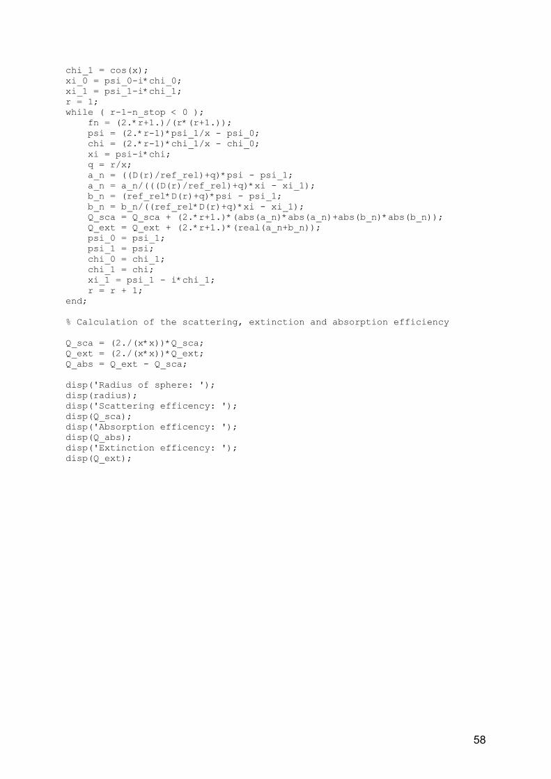
58

chi_1 = cos(x); xi_0 = psi_0-i*chi_0; xi_1 = psi_1-i*chi_1; r = 1; while ( r-1-n_stop < 0 ); fn = (2.*r+1.)/(r*(r+1.)); psi = (2.*r-1)*psi_1/x - psi_0; chi = (2.*r-1)*chi_1/x - chi_0; xi = psi-i*chi; q = r/x; a_n = ((D(r)/ref_rel)+q)*psi - psi_1; a_n = a_n/(((D(r)/ref_rel)+q)*xi - xi_1); b_n = (ref_rel*D(r)+q)*psi - psi_1; b_n = b_n/((ref_rel*D(r)+q)*xi - xi_1); Q_sca = Q_sca + (2.*r+1.)*(abs(a_n)*abs(a_n)+abs(b_n)*abs(b_n)); Q_ext = Q_ext + (2.*r+1.)*(real(a_n+b_n)); psi_0 = psi_1; psi_1 = psi; chi_0 = chi_1; chi_1 = chi; xi_1 = psi_1 - i*chi_1; r = r + 1; end; % Calculation of the scattering, extinction and absorption efficiency Q_sca = (2./(x*x))*Q_sca; Q_ext = (2./(x*x))*Q_ext; Q_abs = Q_ext - Q_sca; disp('Radius of sphere: '); disp(radius); disp('Scattering efficency: '); disp(Q_sca); disp('Absorption efficency: '); disp(Q_abs); disp('Extinction efficency: '); disp(Q_ext);

59

Appendix C

Matlab code for the calculations of the argon flow at the inlet for a residence time of 1 second: function [x] = volumeflow(n_tube,ra,m_zno); % Masterthesis 06/07 - ETH Zurich - Sophia Haussener %% Calculates the argon mass flow at the inlet (standard) for a residence % time in the reactor of 1s at 2000K %% Input: tube number, absorber radius [m], total mass flow of ZnO [kg/min] % Output: Ar volume flow at inlet m_zno = m_zno/n_tube/60; % ZnO mass flow per tube tau = 1; % residence time in reactor at average reactor temperature T = 2000; % average reactor temperature R = 8.314; % ideal gas constant T_0 = 273; % reference temperature p_0 = 101325; % 1 atm l = 0.2; % reactorlength roh_0 = 5660; % ZnO bulk density ra = ra - 0.003; % reduce to inner radius V_ar = (l*pi*ra^2-tau*(m_zno/roh_0))/tau; m_ar = V_ar*(p_0*0.03995/(R*T)); V_ar_s = m_ar/(p_0*0.03995/(R*T_0)); V_frac = (m_zno/roh_0)/(V_ar + (m_zno/roh_0)); roh = roh_0*V_frac; % effective ZnO density Y = m_zno/(m_zno+m_ar); disp('Argon volumetric flowrate at inlet [m^3/s]: '); disp(V_ar_s); disp('Argon volumetric flowrate at inlet [l/min]: '); disp(V_ar_s*60000); disp('Argon volumetric flowrate at 2000K [m^3/s]: '); disp(V_ar); disp('Argon volumetric flowrate at 2000K [l/min]: '); disp(V_ar*60000); disp('Volume fraction ZnO: '); V_frac disp('Mass fraction ZnO: '); Ydisp('Effective density of ZnO [m^3/kg]: '); roh

60

Appendix D

Fluent code for the udf (user defined function) to calculate temperature dependent properties of the single species and the mixture as well as the sink term: /* Fluent UDFs */ /* Sophia Haussener - Masterthesis - 2006/07 */ /* */ /* Second block of constant values and scattering */ /* UDF has to be changed for different cases! */

#include "udf.h" /* Constant variables */ /* Second block dependent on initial condition! */ real tau = 1.0; real R = 8.314; real Ea = 356000.0; real k0 = 4.0e9; real T_ref = 500.0; real hr = 470600.0; real mass_frac_0 = 0.7297; real v_gas = 1.487/60.0; /* at 273K */ real m_zno = 7.16/(60.0*1000.0); real v_zno = 1.1611e-4; real radius = 0.02 - 0.003; real len = 0.05881;

/* Fluent UDF to write quantity to memory */ DEFINE_ADJUST(adjust,d)

Thread *t; cell_t c; real conv, area, cp_zno; d = Get_Domain(1); area = 3.14159265359*radius*radius; thread_loop_c(t,d)

begin_c_loop(c,t) C_UDMI(c,t,0) = 1.0-exp(-k0 *exp(-Ea/(R*C_T(c,t)))*tau); /* write conversion to memory */ C_UDMI(c,t,1) = mass_frac_0*exp(-k0*exp(-Ea/(R*C_T(c,t)))*tau); /* write ZnO mass fraction to memory */ cp_zno = (24.456+3.4987e-2*C_T(c,t)-3.9761e-5*pow(C_T(c,t),2)+2.0374e-8*pow(C_T(c,t),3)-3.7848e-12*pow(C_T(c,t),4))/0.08138; conv = 1 - exp(-k0*exp(-Ea/(R*C_T(c,t)))*tau); C_UDMI(c,t,2) = -(v_gas*0.03995/22.4*520*(C_T(c,t)-T_ref))/area/len; /* write sink term for argon heating to memory */ C_UDMI(c,t,3) = -(m_zno*cp_zno*(C_T(c,t)-T_ref))/area/len; /* write sink term for zinc-oxide heating to memory */ C_UDMI(c,t,4) = -(conv*hr*m_zno/0.08138)/area/len; /* write sink term for reaction to memory */ end_c_loop(c,t)

61

/* Fluent UDF for temperature dependent properties for core fluid */ DEFINE_PROPERTY(k,c,t) /* conductivity */

real mass_frac3, temp, conv, k, k_ZnO, k_Zn, k_O2, k_Ar; temp = C_T(c,t); conv = 1-exp(-k0*exp(-Ea/(R*temp))*tau); mass_frac3 = mass_frac_0*(1-conv); k_ZnO = 0.2; k_Zn = 0.03; k_O2 = 0.126; k_Ar = (0.000633*pow(temp,0.6221))/(1+(70/temp)); k = mass_frac3*k_ZnO + mass_frac_0*conv*(65.39/81.38)*k_Zn + mass_frac_0*conv*(0.5*31.89/81.38)*k_O2 + (1-mass_frac_0)*k_Ar; return k;

DEFINE_PROPERTY(mu,c,t) /* viscosity */

real mass_frac4, temp, conv, mu, mu_ZnO, mu_Zn, mu_O2, mu_Ar; temp = C_T(c,t); conv = 1-exp(-k0*exp(-Ea/(R*temp))*tau); mass_frac4 = mass_frac_0*(1-conv); mu_ZnO = 6.0e-5; mu_Zn = 6.334e-5; mu_O2 = 6.371e-5; mu_Ar = (9.121e-7*pow(temp,0.60529))/(1+(83.24/temp)); mu = mass_frac4*mu_ZnO + mass_frac_0*conv*(65.39/81.38)*mu_Zn + mass_frac_0*conv*(0.5*31.89/81.38)*mu_O2 + (1-mass_frac_0)*mu_Ar; return mu;

DEFINE_PROPERTY(roh,c,t) /* density */

real mass_frac5, temp, conv, roh, roh_ZnO, roh_Zn, roh_O2, roh_Ar; temp = C_T(c,t); conv = 1-exp(-k0*exp(-Ea/(R*temp))*tau); mass_frac5 = mass_frac_0*(1-conv); roh_ZnO = 5660*v_zno; roh_Zn = 0.06539*100000/(R*temp); roh_O2 = 0.03189*100000/(R*temp); roh_Ar = 0.03995*100000/(R*temp); roh = mass_frac5*roh_ZnO + mass_frac_0*conv*(65.39/81.38)*roh_Zn + mass_frac_0*conv*(0.5*31.89/81.38)*roh_O2 + (1-mass_frac_0)*roh_Ar; return roh;

/* Fluent UDF for sink term */ DEFINE_SOURCE(sink,c,t,dS,eqn)

real sink, conv, area, cp_zno; area = 3.14159265359*radius*radius; cp_zno = (24.456+3.4987e-2*C_T(c,t)-3.9761e-5*pow(C_T(c,t),2)+2.0374e-8*pow(C_T(c,t),3)-3.7848e-12*pow(C_T(c,t),4))/0.08138; conv = 1 - exp(-k0*exp(-Ea/(R*C_T(c,t)))*tau); sink = -(v_gas*0.03995/22.4*520*(C_T(c,t)-T_ref)+m_zno*cp_zno*(C_T(c,t)-T_ref)+conv*hr*m_zno/0.08138)/area/len;

62

return sink;

/* Fluent UDF for temperature dependent properties for air */ DEFINE_PROPERTY(k_air,c,t) /* conductivity of air */

real temp, k_air; temp = C_T(c,t); k_air = (0.00031417*pow(temp,0.7786))/(1-(0.7116/temp)+(2121.7/(temp*temp))); return k_air;

DEFINE_PROPERTY(mu_air,c,t) /* viscosity of air */

real temp, mu_air; temp = C_T(c,t); mu_air = (1.425e-6*pow(temp,0.5039))/(1+(108.3/temp)); return mu_air;

/* ------------------------------------------------------------- */ /* The following only for completeness, not used in the 2D model */ /* ------------------------------------------------------------- */ /* Fluent UDF for absorption and scattering coeff. of the core fluid */ DEFINE_GRAY_BAND_ABS_COEFF(absorption,c,t,nb)

real abs_coeff; real mass_frac; int i = 0; /* mass fraction of ZnO */ mass_frac = C_YI(c,t,i); /* printf("ZnO massfraction: %d\n",mass_frac);*/ /* printf("Nr1: %d\n", C_YI(c,t,1));*/ /* printf("Nr2: %d\n", C_YI(c,t,2));*/ /* printf("Nr3: %d\n", C_YI(c,t,3));*/ switch (nb)

case 0 : abs_coeff = mass_frac*3750; break; case 1 : abs_coeff = mass_frac*3750; break; case 2 : abs_coeff = mass_frac*62.5; break; case 3 : abs_coeff = 0.0; break;

return abs_coeff;

DEFINE_DOM_SOURCE(scattering,c,t,ni,nb,emission,in_scattering,abs_coeff,scat_coeff)

double mass_frac; int i = 0; /* mass fraction of ZnO */ mass_frac = C_YI(c,t,i); switch (nb)

case 0 : *scat_coeff = 3000.0; break; case 1 : *scat_coeff = 62.5; break; case 2 : *scat_coeff = 62.5; break; case 3 : *scat_coeff = 0.0; break;

63

/* Fluent UDF for diffusivity */ DEFINE_DIFFUSIVITY(diffusivity,c,t,i)

double temp, diff; temp = C_T(c,t); switch (i)

case 0 : diff = 1e-9; break; /* Ar-ZnO */ case 1 : diff = 5.31685e-10*pow(temp,1.793); break; /* Ar-Zn */ case 2 : diff = 5.41609e-9*pow(temp,1.5); break; /* Ar-O2 */ case 3 : diff = 5.04032e-9*pow(temp,1.5); break; /* Ar-Ar */

return diff;

64

Appendix E

Matlab code for the calculations of the position of the absorber tubes and their dimensions:

function [x] = circle(n_tube,rc,rj); % Masterthesis 06/07 - ETH Zurich - Sophia Haussener %% Calculates and plots the position of 3 or 5 absorber tubes on a circle in % front of window - rc and rj (distance to window) constant %% Input: tube number, cavity radius, distance to window "rj" % Output: position of absorber tube centerpoint, absorber tube radius s_t = 1; [t1,t2] = circle(0,0,rc,rc,0,rj); s_l = asin(t2/rj)/(2*pi)*2*rj*pi*2; ra = [0.001:0.0001:0.1]; j = 1; s_t = 0; while (s_t < s_l); [a1,a2] = circle(rc,0,rj,rc-rj,0,ra(j)); s_t = n_tube*asin(a2/rj)/(2*pi)*2*rj*pi*2 + (n_tube+1+2)*0.006; j = j+1; end; disp('Radius of absorbtion tube: ') disp(ra(j)); disp('Positions of aborber tube centerpoints: ') [xp,yp] = position(rj,n_tube,rc,ra(j)) plot_circle(xp,yp,rc,ra(j),rj,n_tube);

function q = plot_circle(xp,yp,rc,ra,rj,n_tube); % Masterthesis 06/07 - ETH Zurich - Sophia Haussener %% Plots the cavity, absorber tubes and the circle on which the centerpoints % of the absorber tubes lie %% Input: position of absorber tube centerpoint and radius of cavity ans % absorber tubes % Output: plot teta = [0:(2*pi/1440):2*pi]; [t1,t2] = circle(0,0,rc,rc,0,rj); teta_tot = asin(t2/rj); teta_less = [0:(2*pi/180):2*pi]; %figure; hold on; for j = 1:n_tube; for v = 1:1441; w = [xp(j) + ra*cos(teta(v));yp(j) + ra*sin(teta(v))]; plot(w(1),w(2),'k-'); m = [xp(j) + (ra-0.003)*cos(teta(v));yp(j) + (ra-0.003)*sin(teta(v))];

65

plot(m(1),m(2),'k-'); hold on; end; end; hold on; for v = 1:1441; main = [rc*cos(teta(v));rc*sin(teta(v))]; plot(main(1),main(2),'k-'); main3 = [(rc+0.003)*cos(teta(v));(rc+0.003)*sin(teta(v))]; plot(main3(1),main3(2),'k-'); end; for v = 1:181; if (teta_less(v) > (pi-teta_tot) && teta_less(v) < (pi+teta_tot)) main2 = [rc+rj*cos(teta_less(v));rj*sin(teta_less(v))]; plot(main2(1),main2(2),'k:'); hold on; end; end;

function [xp,yp] = position(ri,n,rc,ra); % Masterthesis 06/07 - ETH Zurich - Sophia Haussener %% Calculates the centerpoints of the absorber tubes %% Input: radius of line % Output: position of absorber tube centerpoints

[t1,t2] = circle(0,0,rc,rc,0,ri); teta_tot = asin(t2/ri); [a1,a2] = circle(rc,0,ri,rc-ri,0,ra); if (n == 3); teta = asin(a2/ri); delta_teta = teta_tot - teta - 0.006/ri; teta = teta + 0.5*delta_teta; xp(1) = rc-ri; yp(1) = 0; xp(2) = rc - ri*cos(teta); yp(2) = ri*sin(teta); xp(3) = rc - ri*cos(teta); yp(3) = -ri*sin(teta); elseif (n == 4); teta = asin(a2/ri) + 0.003/ri; teta2 = teta + 2*asin(a2/ri) + 0.006/ri; xp(1) = rc - ri*cos(teta); yp(1) = ri*sin(teta); xp(2) = rc - ri*cos(teta2); yp(2) = ri*sin(teta2); xp(3) = rc - ri*cos(teta); yp(3) = -ri*sin(teta); xp(4) = rc - ri*cos(teta2); yp(4) = -ri*sin(teta2); else teta = asin(a2/ri) + 4*0.006/ri ; delta_teta = 0.25*(teta_tot - teta); teta1 = asin(a2/ri) + 0.006/ri + delta_teta; teta2 = teta1 + 0.006/ri + 2*delta_teta; xp(1) = rc-ri;

66

yp(1) = 0; xp(2) = rc - ri*cos(teta1); yp(2) = ri*sin(teta1); xp(3) = rc - ri*cos(teta1); yp(3) = -ri*sin(teta1); xp(4) = rc - ri*cos(teta2); yp(4) = ri*sin(teta2); xp(5) = rc - ri*cos(teta2); yp(5) = -ri*sin(teta2); end;

function [x,y] = circle(mx_1,my_1,r1,mx_2,my_2,r2); % Masterthesis 06/07 - ETH Zurich - Sophia Haussener %% Calculates the intersection points between two circles % Valid for circles on the x-axis %% Input: x and y point of circle enter and radius: % mx_1,my_1,r_1,mx_2,my_2,r_2 % Output: two intersection points

% general valid: %d = ((mx_2-mx_1)^2+(my_2-my_1)^2); %x(1)= 0.5*(mx_1+mx_2) + (mx_2-mx_1)*(r1^2-r2^2)/(2*d) + (my_2-%my_1)/(2*d)*(((r1+r2)^2-d)*(d-(r2-r1)^2))^0.5; %x(2)= 0.5*(mx_1+mx_2) + (mx_2-mx_1)*(r1^2-r2^2)/(2*d) - (my_2-%my_1)/(2*d)*(((r1+r2)^2-d)*(d-(r2-r1)^2))^0.5; %y(1)= 0.5*(my_1+my_2) + (my_2-my_1)*(r1^2-r2^2)/(2*d) - (mx_2-%mx_1)/(2*d)*(((r1+r2)^2-d)*(d-(r2-r1)^2))^0.5; %y(2)= 0.5*(my_1+my_2) + (my_2-my_1)*(r1^2-r2^2)/(2*d) + (mx_2-%mx_1)/(2*d)*(((r1+r2)^2-d)*(d-(r2-r1)^2))^0.5;

% valid if the circles lie on x-axis x = (r1^2-r2^2+mx_2^2-mx_1^2)/(2*(mx_2-mx_1)); y = r1^2-(x-mx_1)^2; y = sqrt(abs(y));

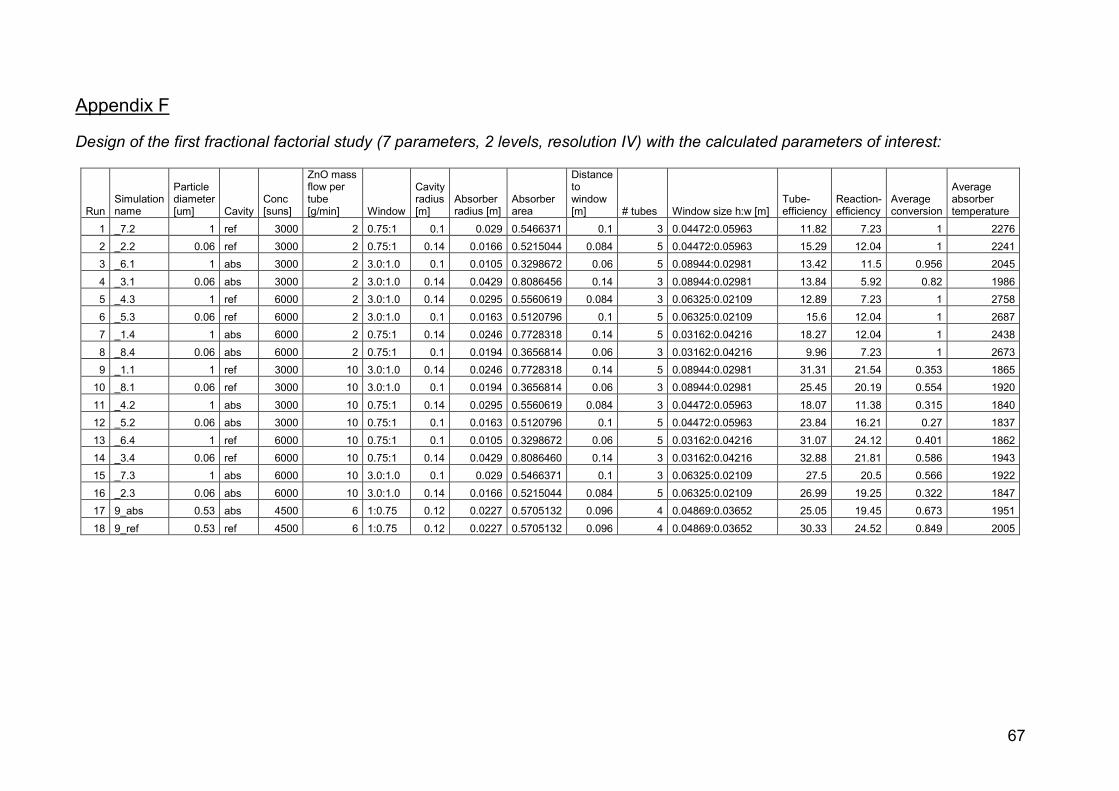
67

Appendix F

Design of the first fractional factorial study (7 parameters, 2 levels, resolution IV) with the calculated parameters of interest:

RunSimulationname

Particlediameter[um] Cavity

Conc[suns]

ZnO massflow pertube[g/min] Window

Cavityradius[m]

Absorberradius [m]

Absorberarea

Distancetowindow[m] # tubes Window size h:w [m]

Tube-efficiency

Reaction-efficiency

Averageconversion

Averageabsorbertemperature

1 _7.2 1 ref 3000 2 0.75:1 0.1 0.029 0.5466371 0.1 3 0.04472:0.05963 11.82 7.23 1 22762 _2.2 0.06 ref 3000 2 0.75:1 0.14 0.0166 0.5215044 0.084 5 0.04472:0.05963 15.29 12.04 1 22413 _6.1 1 abs 3000 2 3.0:1.0 0.1 0.0105 0.3298672 0.06 5 0.08944:0.02981 13.42 11.5 0.956 20454 _3.1 0.06 abs 3000 2 3.0:1.0 0.14 0.0429 0.8086456 0.14 3 0.08944:0.02981 13.84 5.92 0.82 19865 _4.3 1 ref 6000 2 3.0:1.0 0.14 0.0295 0.5560619 0.084 3 0.06325:0.02109 12.89 7.23 1 27586 _5.3 0.06 ref 6000 2 3.0:1.0 0.1 0.0163 0.5120796 0.1 5 0.06325:0.02109 15.6 12.04 1 26877 _1.4 1 abs 6000 2 0.75:1 0.14 0.0246 0.7728318 0.14 5 0.03162:0.04216 18.27 12.04 1 24388 _8.4 0.06 abs 6000 2 0.75:1 0.1 0.0194 0.3656814 0.06 3 0.03162:0.04216 9.96 7.23 1 26739 _1.1 1 ref 3000 10 3.0:1.0 0.14 0.0246 0.7728318 0.14 5 0.08944:0.02981 31.31 21.54 0.353 1865

10 _8.1 0.06 ref 3000 10 3.0:1.0 0.1 0.0194 0.3656814 0.06 3 0.08944:0.02981 25.45 20.19 0.554 192011 _4.2 1 abs 3000 10 0.75:1 0.14 0.0295 0.5560619 0.084 3 0.04472:0.05963 18.07 11.38 0.315 184012 _5.2 0.06 abs 3000 10 0.75:1 0.1 0.0163 0.5120796 0.1 5 0.04472:0.05963 23.84 16.21 0.27 183713 _6.4 1 ref 6000 10 0.75:1 0.1 0.0105 0.3298672 0.06 5 0.03162:0.04216 31.07 24.12 0.401 186214 _3.4 0.06 ref 6000 10 0.75:1 0.14 0.0429 0.8086460 0.14 3 0.03162:0.04216 32.88 21.81 0.586 194315 _7.3 1 abs 6000 10 3.0:1.0 0.1 0.029 0.5466371 0.1 3 0.06325:0.02109 27.5 20.5 0.566 192216 _2.3 0.06 abs 6000 10 3.0:1.0 0.14 0.0166 0.5215044 0.084 5 0.06325:0.02109 26.99 19.25 0.322 184717 9_abs 0.53 abs 4500 6 1:0.75 0.12 0.0227 0.5705132 0.096 4 0.04869:0.03652 25.05 19.45 0.673 195118 9_ref 0.53 ref 4500 6 1:0.75 0.12 0.0227 0.5705132 0.096 4 0.04869:0.03652 30.33 24.52 0.849 2005

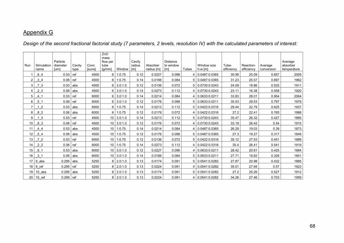
68

Appendix G

Design of the second fractional factorial study (7 parameters, 2 levels, resolution IV) with the calculated parameters of interest:

Run Simulationname

Particlediameter[um]

Cavitytype

Conc[suns]

ZnOmassflow pertube[g/min] Window

Cavityradius[m]

Absorberradius [m]

Distanceto window[m] Tubes

Window sizeh:w [m]

Tube-efficiency

Reaction-efficiency

Averageconversion

Averageabsorbertemperature

1 _6_4 0.53 ref 4500 6 1:0.75 0.12 0.0227 0.096 4 0.0487:0.0365 30.99 25.09 0.857 20052 _3_4 0.06 ref 4500 6 1:0.75 0.14 0.0166 0.084 5 0.0487:0.0365 31.23 25.57 0.697 19623 _7_3 0.53 abs 4500 6 3.0:1.0 0.12 0.0136 0.072 5 0.0730:0.0243 24.09 18.86 0.525 19114 _2_3 0.06 abs 4500 6 3.0:1.0 0.14 0.0273 0.112 4 0.0730:0.0243 23.11 16.38 0.558 19205 _4_1 0.53 ref 6000 6 3.0:1.0 0.14 0.0214 0.084 4 0.0633:0.0211 33.83 28.01 0.954 20646 _5_1 0.06 ref 6000 6 3.0:1.0 0.12 0.0176 0.096 5 0.0633:0.0211 35.53 29.53 0.797 19797 _1_2 0.53 abs 6000 6 1:0.75 0.14 0.0213 0.112 5 0.0422:0.0316 29.44 22.79 0.625 19378 _8_2 0.06 abs 6000 6 1:0.75 0.12 0.0176 0.072 4 0.0422:0.0316 27.2 22.41 0.765 19889 _1_3 0.53 ref 4500 10 3.0:1.0 0.14 0.0213 0.112 5 0.0730:0.0243 35.47 26.32 0.427 1885

10 _8_3 0.06 ref 4500 10 3.0:1.0 0.12 0.0176 0.072 4 0.0730:0.0243 33.19 26.42 0.54 191511 _4_4 0.53 abs 4500 10 1:0.75 0.14 0.0214 0.084 4 0.0487:0.0365 26.29 19.03 0.39 187312 _5_4 0.06 abs 4500 10 1:0.75 0.12 0.0176 0.096 5 0.0487:0.0365 27.3 19.27 0.317 184613 _7_2 0.53 ref 6000 10 1:0.75 0.12 0.0136 0.072 5 0.0422:0.0316 35.12 27.53 0.451 188914 _2_2 0.06 ref 6000 10 1:0.75 0.14 0.0273 0.112 4 0.0422:0.0316 35.4 26.41 0.541 191915 _6_1 0.53 abs 6000 10 3.0:1.0 0.12 0.0227 0.096 4 0.0633:0.0211 28.42 20.81 0.425 188416 _3_1 0.06 abs 6000 10 3.0:1.0 0.14 0.0166 0.084 5 0.0633:0.0211 27.71 19.82 0.326 185117 9_abs 0.295 abs 5250 8 2.0:1.0 0.13 0.0174 0.091 5 0.0541:0.0282 27.87 20.98 0.432 188518 9_ref 0.295 ref 5250 8 2.0:1.0 0.13 0.0224 0.091 4 0.0541:0.0282 35.01 27.94 0.57 192319 10_abs 0.295 abs 5250 8 2.0:1.0 0.13 0.0174 0.091 5 0.0541:0.0282 27.2 20.26 0.527 191220 10_ref 0.295 ref 5250 8 2.0:1.0 0.13 0.0224 0.091 4 0.0541:0.0282 34.26 27.46 0.703 1959

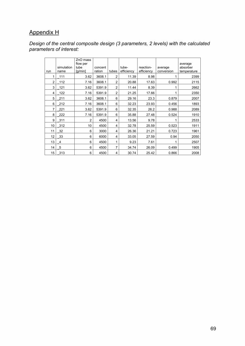
69

Appendix H

Design of the central composite design (3 parameters, 2 levels) with the calculated parameters of interest:

run simulation name

ZnO mass flow per tube [g/min]

concentration tubes

tube-efficiency

reaction-efficiency

average conversion

average absorber temperature

1 _111 3.62 3608.1 2 11.39 8.98 1 23992 _112 7.16 3608.1 2 20.88 17.63 0.992 21153 _121 3.62 5391.9 2 11.44 8.39 1 26624 _122 7.16 5391.9 2 21.25 17.66 1 23505 _211 3.62 3608.1 6 29.16 23.3 0.879 20076 _212 7.16 3608.1 6 32.23 23.93 0.456 18937 _221 3.62 5391.9 6 32.35 26.2 0.988 20898 _222 7.16 5391.9 6 35.88 27.48 0.524 19109 _311 2 4500 4 13.56 9.78 1 2533

10 _312 10 4500 4 32.78 25.59 0.523 191111 _32 6 3000 4 26.36 21.21 0.723 196112 _33 6 6000 4 33.05 27.59 0.94 205013 _4 6 4500 1 9.23 7.61 1 250714 _5 6 4500 7 34.74 26.09 0.499 190515 _313 6 4500 4 30.74 25.42 0.866 2008

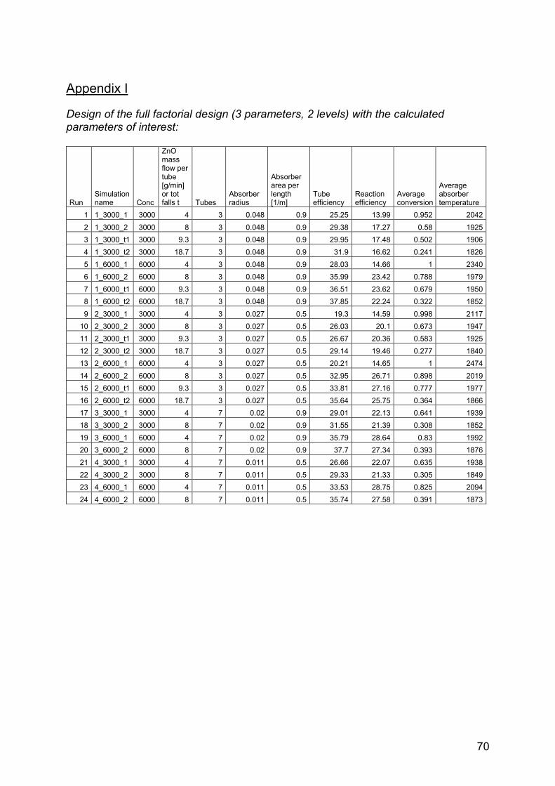
70

Appendix I

Design of the full factorial design (3 parameters, 2 levels) with the calculated parameters of interest:

Run Simulation name Conc

ZnO mass flow per tube [g/min] or tot falls t Tubes

Absorber radius

Absorber area per length [1/m]

Tube efficiency

Reaction efficiency

Average conversion

Average absorber temperature

1 1_3000_1 3000 4 3 0.048 0.9 25.25 13.99 0.952 20422 1_3000_2 3000 8 3 0.048 0.9 29.38 17.27 0.58 19253 1_3000_t1 3000 9.3 3 0.048 0.9 29.95 17.48 0.502 19064 1_3000_t2 3000 18.7 3 0.048 0.9 31.9 16.62 0.241 18265 1_6000_1 6000 4 3 0.048 0.9 28.03 14.66 1 23406 1_6000_2 6000 8 3 0.048 0.9 35.99 23.42 0.788 19797 1_6000_t1 6000 9.3 3 0.048 0.9 36.51 23.62 0.679 19508 1_6000_t2 6000 18.7 3 0.048 0.9 37.85 22.24 0.322 18529 2_3000_1 3000 4 3 0.027 0.5 19.3 14.59 0.998 2117

10 2_3000_2 3000 8 3 0.027 0.5 26.03 20.1 0.673 194711 2_3000_t1 3000 9.3 3 0.027 0.5 26.67 20.36 0.583 192512 2_3000_t2 3000 18.7 3 0.027 0.5 29.14 19.46 0.277 184013 2_6000_1 6000 4 3 0.027 0.5 20.21 14.65 1 247414 2_6000_2 6000 8 3 0.027 0.5 32.95 26.71 0.898 201915 2_6000_t1 6000 9.3 3 0.027 0.5 33.81 27.16 0.777 197716 2_6000_t2 6000 18.7 3 0.027 0.5 35.64 25.75 0.364 186617 3_3000_1 3000 4 7 0.02 0.9 29.01 22.13 0.641 193918 3_3000_2 3000 8 7 0.02 0.9 31.55 21.39 0.308 185219 3_6000_1 6000 4 7 0.02 0.9 35.79 28.64 0.83 199220 3_6000_2 6000 8 7 0.02 0.9 37.7 27.34 0.393 187621 4_3000_1 3000 4 7 0.011 0.5 26.66 22.07 0.635 193822 4_3000_2 3000 8 7 0.011 0.5 29.33 21.33 0.305 184923 4_6000_1 6000 4 7 0.011 0.5 33.53 28.75 0.825 209424 4_6000_2 6000 8 7 0.011 0.5 35.74 27.58 0.391 1873