REPORT DOCUMENTATION PAGE Form Approved

OMB No. 0704-0188

Puouc -poorting curaen 'or this .oiieaion ot information 'S estimated to average l «our per resoor.se. including tne time tor reviewing instructions, searcmng ensung aata sources, jithering and maintaining the data needea. and completing ana reviewing the collection of information Send comments regarding this Burden estimate or any other asoect of this collection )f information including suggestions tor reducing this ouroen to Washington Headquarters Services. Directorate tor information Operations and Reports. 1215 jefferson DAVIS Highway Suite 1204 Arlington /a 22202-1302. and to the Office of Management and Budget. Paperwork Reduction Proiect(0704-Oi88). Washington, OC 20503.

1. AGENCY USE ONLY (Leave blank) 2. REPORT DATE May 07th, 1997

3. REPORT TYPE AND DATES COVERED Final Report S-)-^"? -ia-3/- 9 7

4. TITLE AND SUBTITLE

Theoretical Analysis of Powder Size Distribution

6. AUTHOR(S)

Enrique J. Lavernia

7. PERFORMING ORGANIZATION NAME(S) AND ADDRESS(ES)

Department of Chemical, Biochemical Engineering and Materials Science, University of California, Irvine, CA, 92697-2575

9. SPONSORING/MONITORING AGENCY NAME(S) AND ADDRESS(ES)

AFOSR/NA 110 DUNCAN AVENUE SUITE B115 BULLING AFB DC. 20332-8080

5. FUNDING NUMBERS

Grant no. F49620-97-1-0301

8. PERFORMING ORGANIZATION REPORT NUMBER

10. SPONSORING /MONITORING .AGENCY REPORT NUMBER

11. SUPPLEMENTARY NOTES

79980615 125 12a. DISTRIBUTION /AVAILABILITY STATEMENT

Approved for public release; distribution unlimited.

12b. DlSirs—,

13. ABSTRACT (Maximum 200 words)

The procedure conventionally employed to interpret the experimental sieving data was examined. It was demonstrated that the conventional procedure is inherently flawed in several aspects. Along with several implicit, hard-to-be-justified assumptions associated with it, the conventional graphical representation procedure also failed to address the reliability of the results. To resolve these problems, a new procedure was formulated. Application of the formulated procedure to several sets of sample sieving data reveals that it is capable of extracting the total weight of powders from experimental data, of determining the nature of the size distribution, of establishing the characteristic parameters, and simultaneously, of determining the reliability of the results. It is anticipated that the accomplishment achieved in the present study will generate significant impact on the understanding and the development of powder related processing technologies, including conventional powder metallurgy, conventional spray atomization, and novel spray processing techniques such as spray atomization and deposition, plasma spray forming, and thermal spray forming.

14. SUBJECT TERMS

powder size distribution; sieving data; interpretation procedure

17. SECURITY CLASSIFICATION OF REPORT UNCLASSIFIED

18. SECURITY CLASSIFICATION OF THIS PAGE UNCLASSIFIED

19. SECURITY CLASSIFICATION OF ABSTRACT UNCLASSIFIED

15. NUMBER OF PAGES 32

16. PRICE CODE

20. LIMITATION OF ABSTRACT

UL

NSN 7540-01-280-5500 Standard Form 298 ;Rev 2-89) Pr-scrroed bv -NS. ^td J 39- '8 29(3-'J2

11 MAY rggtf

FINAL REPORT \l^ AFRL-SR-BL-TR-98

t

THEORETICAL ANALYSIS OF POWDER SIZE

DISTRIBUTION

Grant Number: F49620-97-1-0301 - Cumulatrive Funds Awarded: $16,078. £

Period of Performance: 05/01/97 to 12/31/97 S

Submitted to: - C Dr. C.I. CHANG

Director of Aerospace and Materials Sciences Air Force Office of Scientific Research ,

AFOSR/NA 110 DUNCAN AVENUE SUITE B115

BOLLING AFB DC. 20332-8080 ::

Submitted by: Enrique J. Lavernia, Professor and Chair

Department of Chemical, Biochemical Engineering and Materials Science

University of California, Irvine, California, 92697-2575

May 07th, 1997

^

-C'

DTIC QTJALTTY INSPECTED 3

PREFACE

This final report covers the work accomplished during the period from May

1, 1997 to December 31, 1997 under the Air Force Office of Scientific Research

(AFOSR) contract F49620-97-1-0301.

Knowledge of the powder size distribution is essential to characterize a

collection of powders (either experimental samples or commercial products),

and informative to optimize the processing parameters in many powder

related manufacturing techniques, both conventional and novel. Sieving

analysis is a well-established technique to characterize the powder size

distribution. Nevertheless, accurate information on the powder size

distribution necessitates an appropriate procedure to interpret the

experimentally obtained sieving data. To that effect, the conventional

procedure was scrutinized in the present study. It was demonstrated that the

conventional procedure is inherently flawed in several aspects. Along with

several implicit, hard-to-be-justified assumptions associated with it, the

conventional graphical representation procedure also failed to address the

reliability of the results. To resolve these problems, a new procedure was

formulated. Application of the formulated procedure to several sets of

sample sieving data reveals that it is capable of extracting the total weight of

powders from experimental data, of determining the nature of the size

distribution, of establishing the characteristic parameters, and

simultaneously, of determining the reliability of the results. It is anticipated

that the accomplishment achieved in the present study will generate

significant impact on the understanding and the development of powder

related processing technologies, including conventional powder metallurgy,

conventional spray atomization, and novel spray processing techniques such

as spray atomization and deposition, plasma spray forming, and thermal

spray forming.

XOTQPAlOTlHCfflOTSD»

TABLE OF CONTENTS PREFACE i LIST OF PUBLICATIONS iii CHAPTER 1. INTRODUCTION 1 CHAPTER 2. OVERVIEW 2

2.1. Graphical representations 2 2.2. Logarithmic-normal distribution 2 2.3. Curve fitting in graphical representations 3

2.3.1. Histogram and size frequency curves 4 2.3.2. Cumulative plot 4 2.3.3. Probability paper plot 5

CHAPTER 3. PROBLEMS ASSOCIATED WITH GRAPHICAL REPRESENTATION PROCEDURE 6 3.1. Removal of coarse/fine powders 6 3.2. Substitution by truncated distribution 7 3.3. Reliability 8 3.4. Difficulty in determining reliability 10 3.5. Artificial distribution 10

CHAPTER 4. PROPOSED APPROACH 12 4.1. Effect of removal of coarse powders 12

4.1.1. Mathematical formulation 12 4.1.2. Selection of governing equation for curve fitting 13 4.1.3. Realization of curve fitting 14 4.1.4. Applications 15

4.2. Effect of dust separation by cyclone 24 4.2.1. Governing equations 25 4.2.2. Evaluation of the effect of Dmin 26

CHAPTER 5. SUMMARY 28 REFERENCES 29 APPENDIX 1. HONORS AND AWARDS 30 APPENDIX 2. PERSONNEL 32

li

LIST OF PUBLICATIONS resulting from AFOSR Grant no. F49620-97-1-0301

"Analysis of Sieving Data in Reference to Powder Size Distribution", Bing Li and E.J. Lavernia, Ada Materialia, vol. 46, no. 2, pp. 617-629 (1998).

Ill

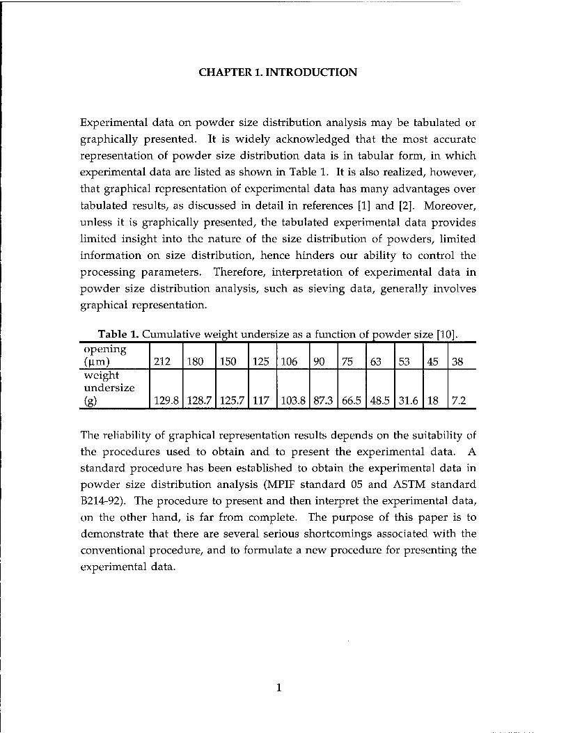
CHAPTER 1. INTRODUCTION

Experimental data on powder size distribution analysis may be tabulated or graphically presented. It is widely acknowledged that the most accurate representation of powder size distribution data is in tabular form, in which experimental data are listed as shown in Table 1. It is also realized, however, that graphical representation of experimental data has many advantages over tabulated results, as discussed in detail in references [1] and [2]. Moreover, unless it is graphically presented, the tabulated experimental data provides limited insight into the nature of the size distribution of powders, limited information on size distribution, hence hinders our ability to control the processing parameters. Therefore, interpretation of experimental data in powder size distribution analysis, such as sieving data, generally involves graphical representation.

Table 1. Cumulative weight undersize as z i function of powder size [10]. opening (Urn) 212 180 150 125 106 90 75 63 53 45 38 weight undersize

(g) 129.8 128.7 125.7 117 103.8 87.3 66.5 48.5 31.6 18 7.2

The reliability of graphical representation results depends on the suitability of the procedures used to obtain and to present the experimental data. A standard procedure has been established to obtain the experimental data in powder size distribution analysis (MPIF standard 05 and ASTM standard B214-92). The procedure to present and then interpret the experimental data, on the other hand, is far from complete. The purpose of this paper is to demonstrate that there are several serious shortcomings associated with the conventional procedure, and to formulate a new procedure for presenting the experimental data.

CHAPTER 2. OVERVIEW

It is helpful to describe, at first, the graphical representations generally

employed in practice, and the most widely used logarithmic-normal size

distribution, before proceeding to address the problems associated with the

conventional procedure in graphical representations.

2.1. Graphical representations

Graphical representations of experimental data in powder size distribution

analysis include [1]:

1). histograms presenting frequency of occurrence versus size range,

2). size frequency curve presenting frequency of occurrence as a function

of powder size, equivalent to a smoothed-out histogram,

3). cumulative plot presenting percent of powders greater (or less) than a

given powder size as a function of powder size, and

4). probability paper plot essentially the same as cumulative plot, except

that the percentage is presented on a probability scale.

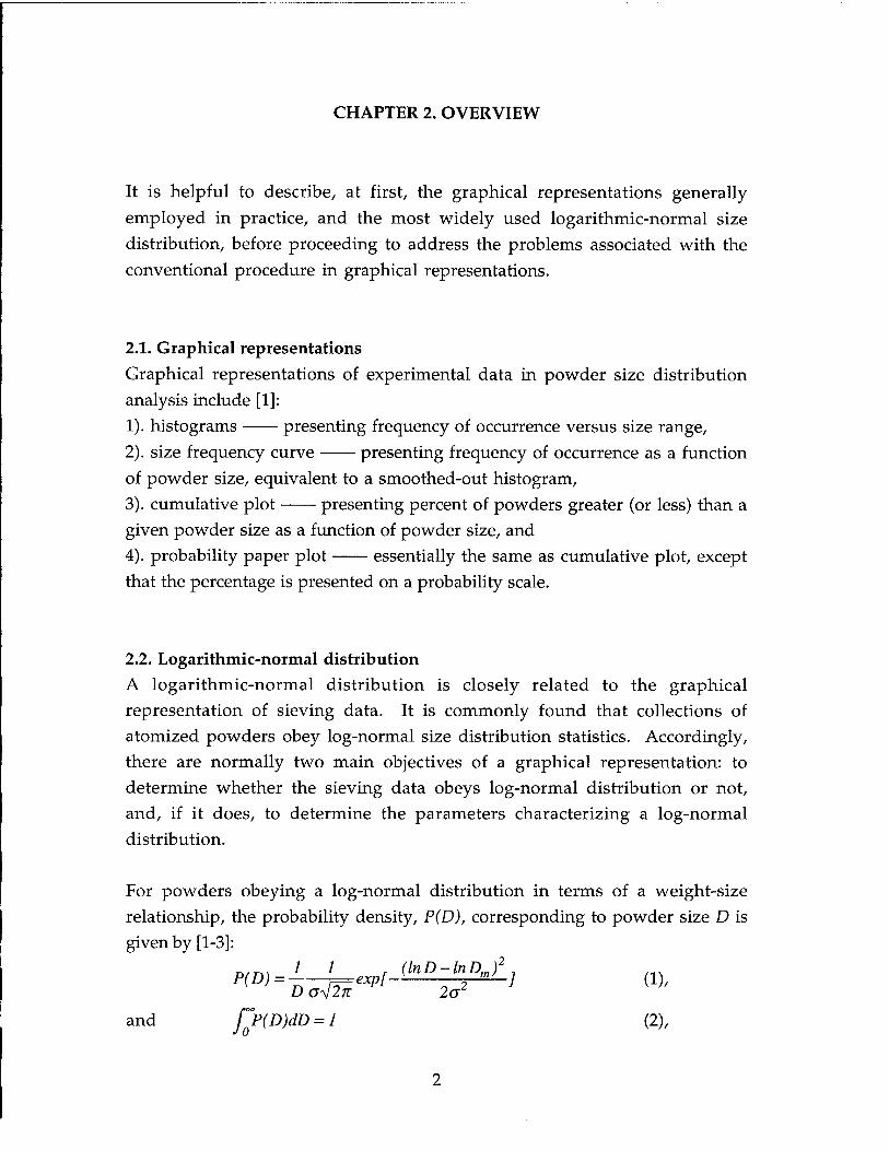
2.2. Logarithmic-normal distribution

A logarithmic-normal distribution is closely related to the graphical

representation of sieving data. It is commonly found that collections of

atomized powders obey log-normal size distribution statistics. Accordingly,

there are normally two main objectives of a graphical representation: to

determine whether the sieving data obeys log-normal distribution or not,

and, if it does, to determine the parameters characterizing a log-normal

distribution.

For powders obeying a log-normal distribution in terms of a weight-size

relationship, the probability density, P(D), corresponding to powder size D is

given by [1-3]:

P(D)=l'xp[J±Rd^l, (1), D o~42n 2o

P(D)dD = 1 (2),

where Dm is the mean mass powder diameter, a is the standard deviation.

The probability density, P(D), corresponding to a powder size D is defined as

P(D)=AWp/AD (3),

where AWp is the weight percentage of powders with size falling in the range

between D and D+AD.

It is evident from equation (1) that powders obeying log-normal distributions

may be characterized by two parameters, the standard deviation, G, and the

mass mean droplet size, Dm. In practice, another three parameters are also

frequently utilized to characterize the powder size distribution. The three

parameters are the characteristic powder sizes, die, dso, and du, under which

16, 50, and 84 wt.% of powders, respectively, are smaller than the stated sizes.

These two characterizing methods are equivalent to each other, since

Dm = d50 (4),

and G = ln(d50/d16) = ln(d84/d50) (5).

Graphically, die, dso, and dg4 may be determined from a cumulative plot or a

probability paper plot, and a and Dm may be determined from a size-frequency

plot. It is worth noting that the magnitudes of these characteristic parameters

may be determined graphically either with or without rigorous curve fitting

involved. Without curve fitting, however, the nature of powder size

distribution is generally unknown. In this case, the characteristic parameters

determined are of no physical significance. In addition, even when the

nature of size distribution is pre-known, curve fitting is necessary to

minimize the extensive experimental errors normally associated with sieving

analysis. Therefore, graphical determination of these parameters should be

proceeded by curve fitting of experimental results.

2.3. Curve fitting in graphical representations

All of the graphical representations involve the weight percentage, rather

than weight, as evident from section 2.1. Conversion of experimentally

determined absolute weight into weight percentage necessitates the

knowledge of the total weight of the powders under analysis. As will be

shown in sections 3 and 4, this parameter is generally unknown. Actually, it

is this fact that complicates the procedure of graphical representation. In this

section, the total weight of the powders is temporarily assumed to be a known

parameter for the convenience of discussion. In this case, both the weight

and weight percentage are readily used in graphical representations and curve

fitting.

2.3.2. Histogram and size frequency curves

In these two plots, curve fitting may be established using equation (1). In

sieving experiments, however, the direct experimental data are weight (or

weight percentage) in a size range, or cumulative weight (or weight

percentage) of powders under a given size, as shown in Table 1. In order to

obtain the probability density, P(D), equation (3) has to be used. However, this

may introduce extensive additional errors into the experimental data by

either of the following two ways. First, if the size interval, AD, in equation (3)

, is selected as the same as that in sieving analysis (for example in Table 1,

they are 32, 30, 25, ,8, and 7 [im in decreasing sequence), AD is generally

too large to be used to accurately calculate P(D) through equation (3). If the

size interval, AD, in equation (3), is selected to be a smaller value, on the

other hand, such as in the range of 2~2 |a,m, subjective interpolation between

the experimental data points would definitely be involved, introducing

unexpected errors. Therefore, curve fitting in either histogram or size

frequency curve plots would not be considered in the present study.

2.3.2. Cumulative plot

Using equation (1), the cumulative percentage, Cp(D), under size D may be

calculated as:

Cp(D)% = fp(D)dD

1 . (InD-lnDJ2

r-L=exp[-[lnU-ln2U^ JdlnD J~ o42n 2a2

j lnD-lnD,„

-==/ ^ exp[-t2]dt

-I In D-ln Dm

= 1 ° exp[-t2/2]dt (6). 2K

J~°

In sieving analysis, powders may be directly characterized by cumulative

weight under size as a function of powder size. When the total weight of the

powders is known, then the cumulative weight percentage under size as a

function of powder size, Cp(D), may be readily obtained. Accordingly,

equation (6) may be employed to curve fit the experimental data.

Unfortunately, the form of equation (6) is so complex such that no attempt

was found in the literature to use it to curve fit the experimental data.

2.3.3. Probability paper plot

By defining a function y=norm(x), for which y and x satisfy

x% = n=fy exp(-t2/2)dt (7), 2K •

equation (6) may be rearranged as lnD-lnDm ^ = norm(C„) (8),

<7

or log D = log Dm+0.434a -norm(C) (8').

In a probability paper plot, the abscissa is the powder size, generally in

logarithmic scale, logD, while the ordinate is the cumulative weight

percentage undersize in probability scale. It is worth noting that the

probability scale is calculated using y=norm(x), or equation (7), i.e., x=50

corresponds to y=0; x=60 corresponds to y=0.25; x=90, y=1.28; x=100, y=oo; x=40,

y=-0.25; x=0, y=-°°; and so on... [4], as shown in Figure 1. Therefore, equation

(8), which indicates that logD is a linear function of norm(Cp), predicts a

straight line for powders obeying log-normal distributions when the

cumulative percentage undersize, Cp, is graphed versus the powder size, D, in

a probability paper plot. This feature is well-known and extensively utilized

to determine whether a collection of powders obeys a log-normal distribution

or not, although its origin is not necessarily always well understood by the

user.

-0.84 -0.25 0.25 0.84 y -2.33 -1.28 T -0.52T 0 ' 0.52 ' 1.28 2.33 1 1 1 1—|—|—|—| 1 1 1

x (%) 1 10 20 30 40 50 60 70 80 90 99

Figure 1. Probability scale y=norm(x).

CHAPTER 3. PROBLEMS ASSOCIATED WITH

GRAPHICAL REPRESENTATION PROCEDURE

In this section, the problems associated with graphical representation

procedures will be discussed. Essentially, all of these problems originate from

the fact that the total weight of powders is generally unknown, which is

closely related to the removal of coarse/fine powders in practical atomization

experiments.

3.1. Removal of coarse/fine powders

It is evident from section 2.1 that all of the graphical representations involve

weight percentage (or frequency), rather than the absolute weight. However,

experimental data generally involve absolute values. Therefore, the first step

of graphical representation is to convert the absolute weight, in the case of

sieving experiments, into weight percentage. This necessitates the knowledge

of the total weight for the powders under analysis. Unfortunately, this

parameter is generally unknown in a lot of pratical situations. This may

appear unusual; however, any detailed examination of the powder size

distribution analysis will indicate that this is generally beyond the capability

of typically used experimental arrangements. Suffice it to point out here that

the powders subjected to experimental size distribution analysis, such as

sieving, are different from the powders formed because of dust separation by

cyclones or/and removal of coarse particles. To make this point more clear,

let us consider a dispersion of powders observing log-normal distribution, as

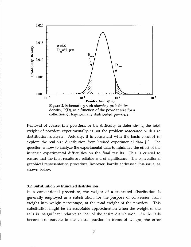
shown in Figure 2. Dust separation by cyclones and removal of coarse

particles truncate the two tails from the bell shape distribution in Figure 2 by

introducing two size-limits, Dm!M, the lower limit, and Dmax, the upper limit.

While the total weight of the truncated distribution may be readily measured

experimentally, the total weight of powders used for conversion from weight

into weight percentage in a graphical representation of sieving data should be

that of the entire powders, rather than the truncated one. Nevertheless, it is

impossible to experimentally measure the total weight of the entire

distribution of powders, since, by definition, the powder size ranges from zero

to infinity for a log-normal distribution.

I» a a

,0 at

X! o u ft.

0.020

0.015 -

0.010

0.005

0.000 10 ° 10 1 10 2

Powder Size (|Xm) Figure 2. Schematic graph showing probability density, P(D), as a function of the powder size for a collection of log-normally distributed powders.

10

Removal of coarse/fine powders, or the difficulty in determining the total

weight of powders experimentally, is not the problem associated with size

distribution analysis. Actually, it is consistent with the basic concept to

explore the real size distribution from limited experimental data [1]. The

question is how to analyze the experimental data to minimize the effect of the

intrinsic experimental difficulties on the final results. This is crucial to

ensure that the final results are reliable and of significance. The conventional

graphical representation procedure, however, hardly addressed this issue, as

shown below.

3.2. Substitution by truncated distribution

In a conventional procedure, the weight of a truncated distribution is

generally employed as a substitution, for the purpose of conversion from

weight into weight percentage, of the total weight of the powders. This

substitution might be an acceptable approximation when the weight of the

tails is insignificant relative to that of the entire distribution. As the tails

become comparable to the central portion in terms of weight, the error

resulting from this approximation may be large. The problem is complicated, however, by the fact that the relative contribution of the tails to the entire distribution, i.e., the criterion for the accuracy of the approximation, generally remains unknown until the total weight of the entire powders is determined.

The conventional procedure is also flawed as a result of another factor. By assuming the weight of a truncated distribution as the total weight of the entire distribution, the experimentally obtained absolute weight may be readily converted into weight percentage. However, a natural result of this assumption is that the cumulative percentage undersize corresponding to Dmax is 100%. Since it is impossible to graph 200% in a probability paper plot, this data point is then ignored. This treatment is difficult to be justified, but widely employed.

3.3. Reliability In the literature, an implicit concept that is widely used involves the assumption that, if the data points obey a log-normal distribution, then the results are reliable. To examine its validity, the experimental data in Table 1 were analyzed using the conventional procedure, with the results shown in Figures 3(a) through (d). The upper limit of powder size, Dmax, was chosen to be 212,150, 90, and 63 \im in Figures 3(a), 3(b), 3(c), and 3(d), respectively. The magnitude of Dmjn was temporarily set to be zero for all cases, as normally treated in conventional procedures. Accordingly, the size range of the truncated distributions are 0~222 |im, 0~150 Jim, 0~90 |im, and 0~63 \im for Figures 3(a) through (d), respectively. Moreover, from Table 1, the weight of these truncated distributions are 129.8,125.7, 87.3, and 48.5 g for Figures 3(a) through (d), respectively. The data were graphed on probability paper plot and curve fitted, with the fitting coefficient, along with the characteristic parameters, summarized in Table 2. It is evident from Figure 3 and Table 2 that introducing different upper limits of powder size, Dmax, does not affect the nature of the size distribution; the data consistently followed log-normal distribution. The characteristic parameters, however, vary extensively with Dmax, rather than remain unchanged, as evident from Table 2. It is important to recall that the ultimate purpose of size distribution analysis is to determine the real size distribution, and the characteristic parameters for the real size

8

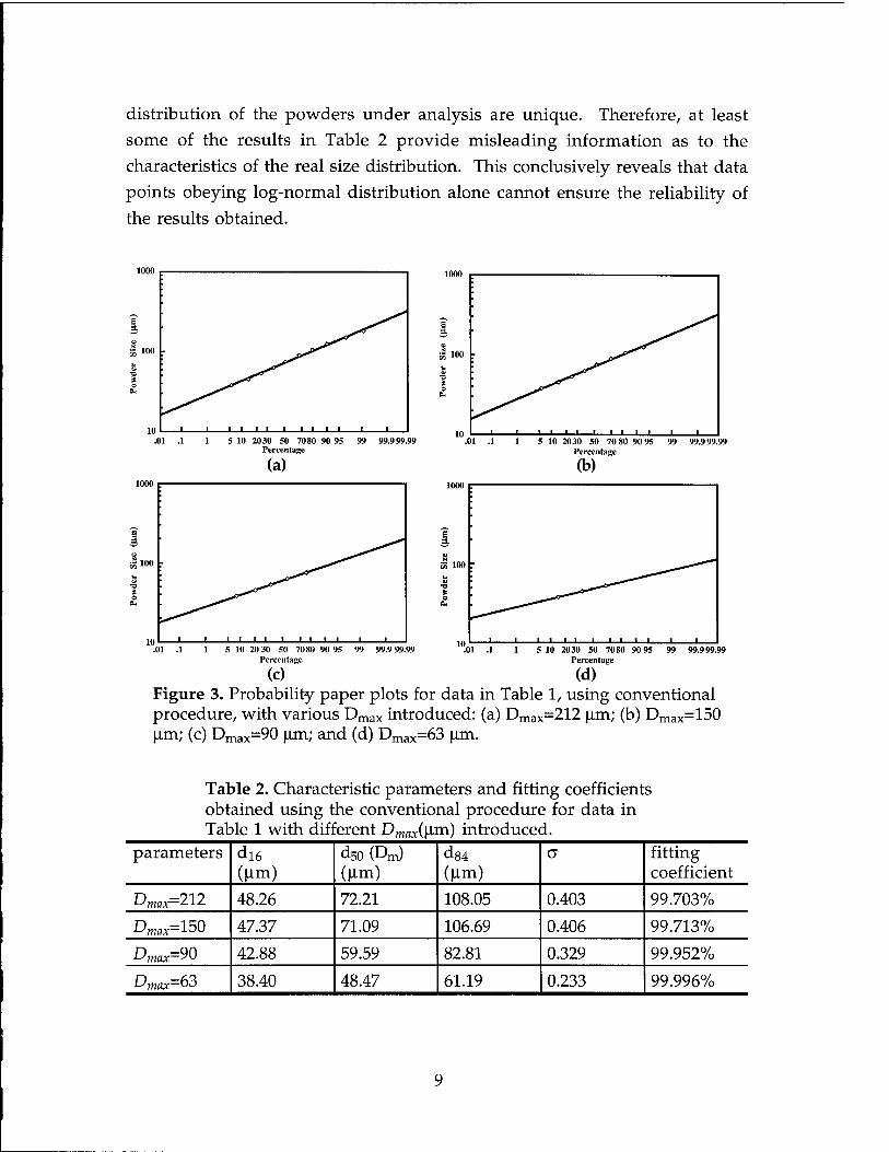
distribution of the powders under analysis are unique. Therefore, at least some of the results in Table 2 provide misleading information as to the characteristics of the real size distribution. This conclusively reveals that data points obeying log-normal distribution alone cannot ensure the reliability of the results obtained.

1000

5 10 2030 50 7080 90 95 99 99.999.99 Percentage

(a)

s loo

5 10 20 30 50 7080 90 95 99 99.9 99.99 Percentage

5 10 2030 50 70 80 90 95 99 99.999.99 Percentage

(b)

5 10 2030 50 7080 90 95 Percentage

(c) (d) Figure 3. Probability paper plots for data in Table 1, using conventional procedure, with various Dmax introduced: (a) Dmax=212 Jim; (b) Dmax=150 fim; (c) Dmax=90 urn; and (d) Dmax=63 |im.

Table 2. Characteristic parameters and fitting coefficients obtained using the conventional procedure for data in Table 1 with different Dmax(\im) introduced.

parameters dl6 (N

dso (Dm) (Jim)

d84 (jim)

o fitting coefficient

>-^max=^-'-^- 48.26 72.21 108.05 0.403 99.703%

LJinax= J-^U 47.37 71.09 106.69 0.406 99.713%

Umax=yv 42.88 59.59 82.81 0.329 99.952%

LJmax=vJ 38.40 48.47 61.19 0.233 99.996%

3.4. Difficulty in determining reliability

Since there are several difficult-to-be-justified assumptions associated with

the conventional procedure, no attempt will be made here to solve, or to

prove it is impossible to solve, the reliability problem under the framework

of conventional graphical representation procedure. Suffice it to point out

that the problem is complicated by the intrinsic difficulty in using a

probability paper plot. This may be briefly described as follows. Considering

the bell shape for a log-normal distributed collection of powders in Figure 2,

as Dmax increases, the results are expected to gradually approach that of the

real size distribution, becoming more and more reliable. This feature might

enable one to judge the reliability of the results obtained. Unfortunately, this

idealized situation is rarely realized in a probability paper plot. As Dmax

deviates from the mean mass diameter, Dm (which means Dmax increases), the

experimental error in the data points will be more and more exaggerated,

such that a minor experimental error associated with the data points

corresponding to large D values would completely change the final results [5].

This could only be avoided by having the data points "weighted" (i.e.,

evaluating the importance of the data points) before graphical representation,

as discussed in detail in reference [5]. Calculation and assignment of the

"weight" for each data point, however, requires a knowledge of the weight

percentage corresponding to each data point, which necessitates a knowledge

of the total weight of the powders [5]. In the conventional procedure, the total

weight of the powders is substituted using the truncated distribution. The

appropriateness of this substitution is, in turn, determined by the reliability of

the results obtained.

3.5. Artificial distribution

The effect stemming from removal of coarse/fine powders on the final

results was addressed by Irani [1, 6] from another point of view. According to

Irani [1, 6], because of the removal of coarse/fine powders, the data points in a

probability paper plot asymptotically approach a line parallel to the abscissa

(the probability scaled axis), rather than fall onto a straight line as expected.

To eliminate or minimize the effect of removal of coarse/fine powders, Irani

[1, 6] suggested that the total weight should be a value greater than the weight

of the corresponding truncated distribution. To determine this value, a

10

reiteration method is employed: assuming a total weight, converting weight into weight percentage based on the assumed total weight, then graphing the converted weight percentage on a probability paper plot versus powder size, and assuming a new total weight and so on, until the data graphed on the probability paper plot satisfactorily fall onto a straight line.

This method, however, has three drawbacks. Firstly, as discussed in section

3.3, data points falling onto a straight line alone does not ensure that the results are reliable. Although the discussion in section 3.3 is under the assumption that the total weight of powders may be substituted by that of the truncated distribution, it is generally true that data points obeying log-normal distribution alone does not assure the reliability of the results, as will be shown in section 4.4. Secondly, the intrinsic difficulty associated with probability paper plot cannot be solved using this method, and hence still affects this method. Finally, this method failed to formulate any equations in determining the total value of powders from curve fitting the experimental data, rendering the entire procedure dubious.

11

CHAPTER 4. PROPOSED APPROACH

As evident from the above discussion, along with several implicit, hard-to-

be-justified, assumptions, the conventional graphical representation

procedure failed to address the reliability of its results. In the following

sections, a new procedure will be formulated. The proposed procedure is

capable of extracting the total weight of powders from experimental data, of

determining the nature of size distribution, of characterizing the characteristic

parameters, and simultaneously, of determining the reliability of its results.

4.1. Effect of removal of coarse powders

In this section, with Dm/M being temporarily set to be zero, only the effect of

Dmax will be considered. The effect of introducing the lower limit of powder

size into the distribution will be discussed in section 4.2.

4.1.1. Mathematical formulation

Equations (l)-(8) correlate powder size with probability (equation (1)), or

cumulative weight percentage under size (equations (6) and (8)).

Experimental data, however, are absolute weight and powder size (refer to

Table 1). This necessitates development of equations directly correlating the

powder size with the absolute weight. The development of these equations

may be readily accomplished by incorporating the total weight of powders

into the analysis in equations (l)-(8).

Assuming the total weight to be Wf, the cumulative weight percentage

undersize D may be calculated as Cp(D)% = Wmder(D)/Wt (9),

where Wunder(D) is the cumulative weight undersize D. When Dmin = 0,

Wunder(D) is equivalent to the experimentally obtained cumulative weight

undersize, Wfnder(D). Substituting equation (9) into equation (8) yields

logD = logDm + 0.434(7 ■ norm(100 W^er(D)} (1Qy

Similarly, substituting equation (9) into equation (6) gives:

12

w, ■I JnD-lnDm

'under(D) = Wt -j= f^ exp(-t2 /2)dt (11).

When the total weight is known, equations (10) and (11) are essentially

equivalent to equations (6) and (8). In this case, development of equations

(10) and (11) is of little significance. When the total weight is unknown,

however, these two sets of equations are totally different. While equations (6)

and (8) may not be utilized to curve fit the experimental data (absolute value),

equations (10) and (11) can. More importantly, equations (10) and (11) enables

extraction of the unknown total weight of powders, Wt, by curve fitting the

sieving experimental data.

4.1.2. Selection of governing equation for curve fitting

In the last section, two equations were developed to correlate the powder size

with the cumulative weight undersize: equation (10) which curve fits D as a function of Wfnder(D); and equation (11) which curve fits W„nder(D) as a

function of D. Mathematically, equation (10) is equivalent to equation (11).

However, experimental data is unavoidably associated with some errors,

making these two equations different from each other in terms of curve

fitting. In the present study, equation (11) is uniquely selected to be the

governing equation in curve fitting because of the following two reasons.

Firstly, in curve fitting, if the governing equation is selected to be y=f(x), then

it is generally assumed that the independent variable, x, is known to be

without error [7]. All the errors are in the dependent variable y [7]. In a

sieving experiment, the powder size D is generally predetermined, i.e., free of

error. The experimental error normally arises from the measurement of the cumulative weight undersize W^nder(D). Accordingly, compared with

equation (10), equation (11), which expresses W^^D) as a function of D, is

more suitable to be employed as the governing equation.

Secondly, in curve fitting, it is generally assumed that the errors associated

with the dependent variable, y, are random [7]. In a sieving experiment, the

error arising from the measurement of the cumulative weight undersize may

be reasonably taken to be random. Therefore, selecting equation (11) as the

governing equation is consistent with the above assumption in curve fitting.

13

If equation (10) is used, on the other hand, W^^iD) would be taken as

without error. Instead, any errors arising from W,fndei.(D) would be evaluated

in terms of D. This makes the error no longer random, as elucidated as

follows. It is evident from Figure 1 that, as x% deviates gradually from 50%,

y=nortn(x) increases (positive) or decreases (negative) more and more rapidly.

Suppose there is a deviation Ax in the independent variable x, the

corresponding deviation in y would depend on the value of x. Let the

deviation in y be Ay I 50 for x%=50%, it would become 15Ay 150 if x%=99% (or

2%), and 28Ay I 50 if x%=99.5% (or 0.5%), and so on, progressively [5]. The

situation discussed here applies to equation (10) by simply substituting

(logD-logDm)/0.434a as y, and 100W^nder(D)/Wt as x. If any errors

originating from 100W^nder(D)/Wt, or from W^nder(D), are evaluated in terms

of (logD - logDm)/0.434a, or D, the results would be dependent on the

magnitude of 100W^nder(D)/Wt. The larger 100W^nder(D)/Wt, the larger the

error. Accordingly, if the errors in 100W„nder(D)/Wt or W^nder(D) are random,

the evaluated errors in terms of (logD - logDm)/0.434a, or D, would no

longer be random. In this case, the experimental point should be "weighted"

(i.e., evaluating the importance of the data points) before curve fitting [5, 7].

Calculation and assignment of the "weight" for each data points, however,

requires the knowledge of the weight percentage corresponding to each data

point, which necessitates the knowledge of the total weight of the powders [5].

Unfortunately, the latter, i.e., the total weight of the powders, is a variable to

be determined, making the assignment of the weight impossible.

Finally, a remark should be made regarding the conventional probability

paper plot. Since one axis of this plot is in probability scale, which is

y = norm(x), the error would be analyzed in terms of D , or

norm[100W^nder(D)/Wt], rather than 100W^nder(D)/Wt, or WEmdJD).

Accordingly, curve fitting in probability paper plot always encounters the

problem associated with equation (10). This is the reason behind the intrinsic

difficulty in the probability paper plot approach mentioned earlier.

4.1.3. Realization of curve fitting

It is evident that equation (11) is, at least, as complex as equation (6). The

practical usefulness of equation (11) relies on the availability of a quick and

14

effective method to curve fit the experimental data using this equation. This

may be realized in a KaleidaGraph software (version 3.0 or above). In the

KaleidaGraph, there are two normal distribution related functions available:

y=nortn(x) and y=inorm(x). Function y=norm(x) was discussed earlier.

Function y=inorm(x) is related to equation (11) as follows:

inorm(x) = -r^f^<xiexp(-t2 /2)dt (12),

which transforms equation (11) into:

wLer(D) = -^-Wtinorm[-lnA] (13).

Governing equation (13) may be defined under the General Curve Fitting

menu in KaleidaGraph Window. To ensure the definition being complete,

the partial derivative of equation (13) relative to Wt, a, and Dm, should be

given. This may be readily accomplished if one notices that

dinorm(x) 100 . x . ,„ .. rexp(-—) (14).

dx -42n 2

4.1.4. Applications

Six sets of sieving data (Tables 1 and 3) from different sources were analyzed

using the formulated procedure, with special attention to its capability of

providing reliable results.

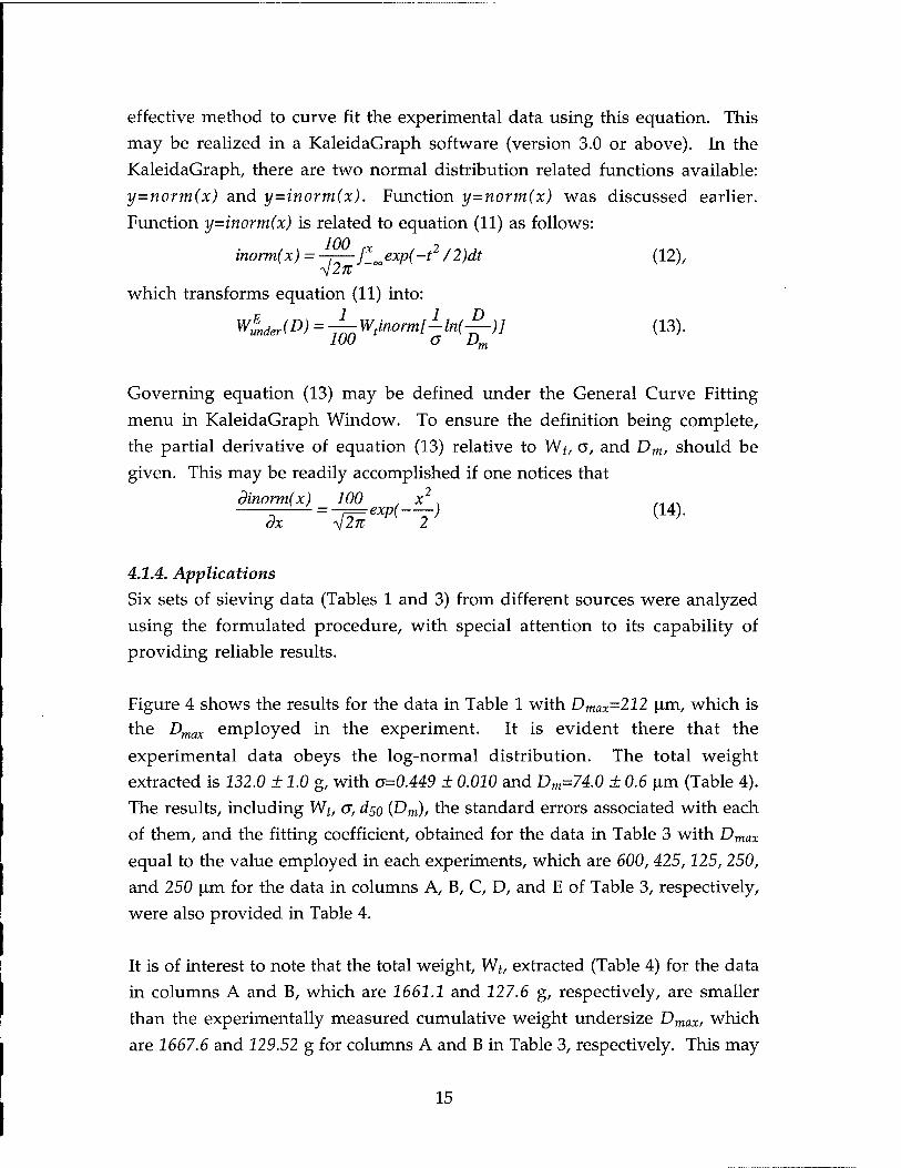
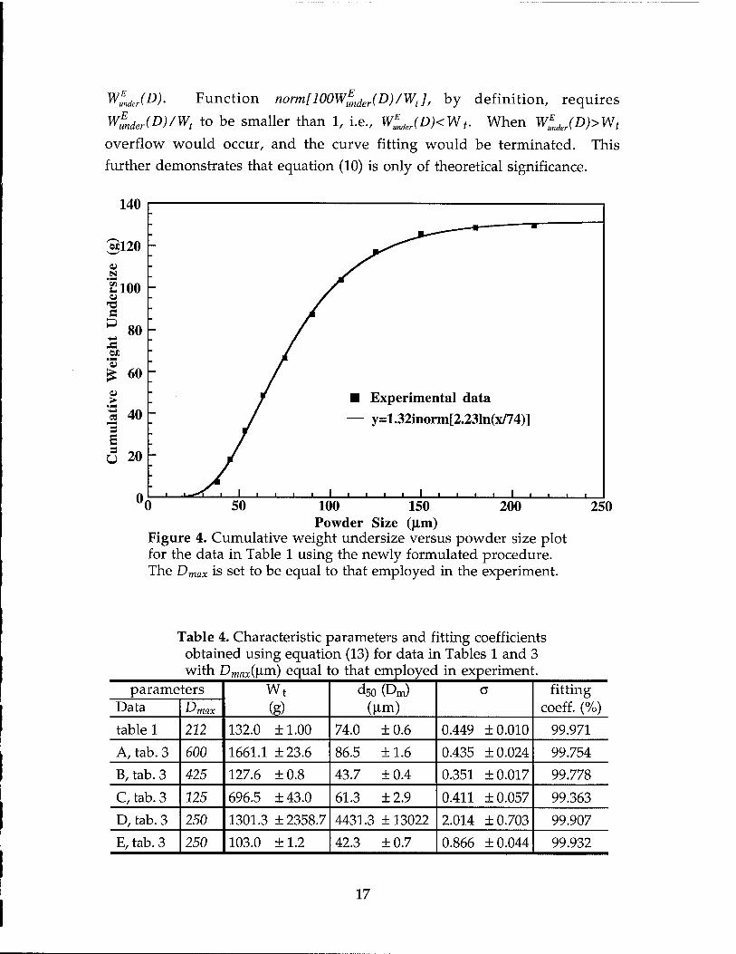
Figure 4 shows the results for the data in Table 1 with Dmax=212 |a,m, which is the Dmax employed in the experiment. It is evident there that the

experimental data obeys the log-normal distribution. The total weight

extracted is 232.0 ± 1.0 g, with a=0.449 ± 0.010 and Dm=74.0 + 0.6 |im (Table 4).

The results, including Wt, o, d^o (Dm), the standard errors associated with each

of them, and the fitting coefficient, obtained for the data in Table 3 with Dmax

equal to the value employed in each experiments, which are 600,425,125, 250,

and 250 urn for the data in columns A, B, C, D, and E of Table 3, respectively,

were also provided in Table 4.

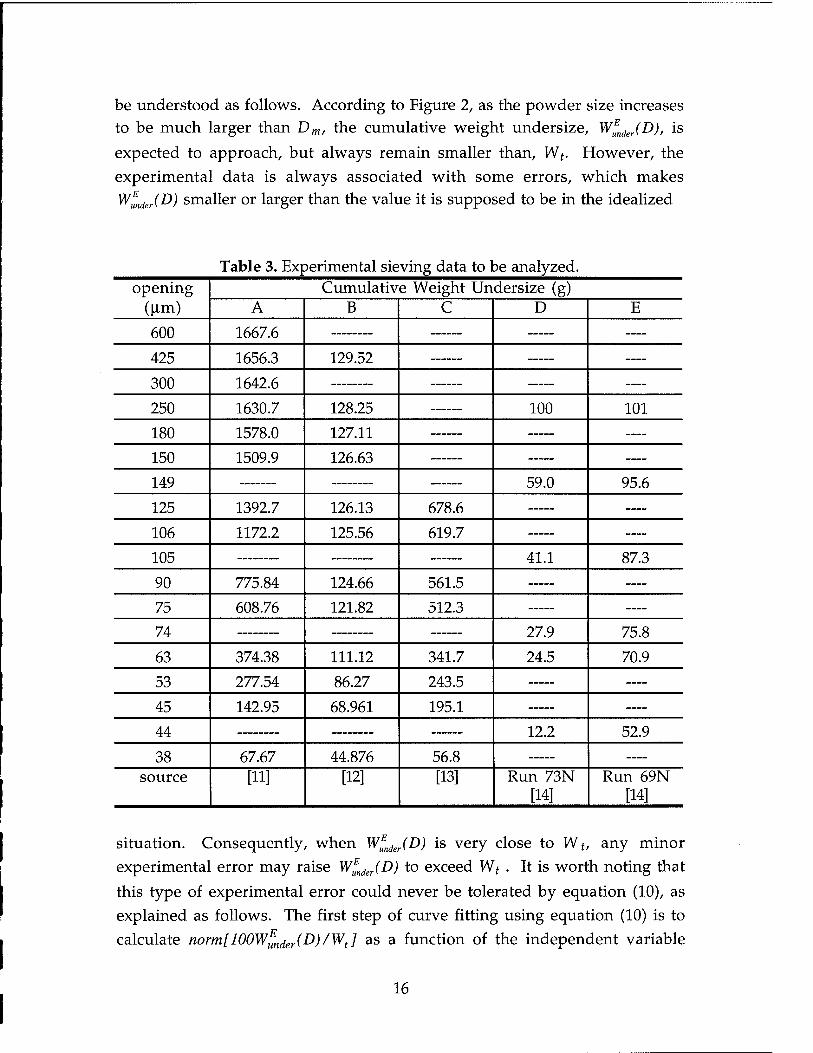
It is of interest to note that the total weight, Wt, extracted (Table 4) for the data

in columns A and B, which are 1661.1 and 227.6 g, respectively, are smaller

than the experimentally measured cumulative weight undersize Dmax, which

are 1667.6 and 129.52 g for columns A and B in Table 3, respectively. This may

15

be understood as follows. According to Figure 2, as the powder size increases

to be much larger than Dm/ the cumulative weight undersize, W^ncler(D), is

expected to approach, but always remain smaller than, Wf. However, the

experimental data is always associated with some errors, which makes

W^nder(D) smaller or larger than the value it is supposed to be in the idealized

Table 3. Experimental sieving data to be analyzed. opening

(|im) Cumulative Weight Undersize (g)

A B C D E

600 1667.6 —

425 1656.3 129.52 —

300 1642.6 —

250 1630.7 128.25 100 101

180 1578.0 127.11 —

150 1509.9 126.63 —

149 59.0 95.6

125 1392.7 126.13 678.6 —

106 1172.2 125.56 619.7 —

105 41.1 87.3

90 775.84 124.66 561.5 —

75 608.76 121.82 512.3 —

74 27.9 75.8

63 374.38 111.12 341.7 24.5 70.9

53 277.54 86.27 243.5 —

45 142.95 68.961 195.1 —

44 12.2 52.9

38 67.67 44.876 56.8 —

source [11] [12] [13] Run 73N [14]

Run 69N [14]

situation. Consequently, when W^nder(D) is very close to W t/ any minor experimental error may raise W^nder(D) to exceed Wt . It is worth noting that

this type of experimental error could never be tolerated by equation (10), as explained as follows. The first step of curve fitting using equation (10) is to calculate norm[100W^nder(D)/Wt] as a function of the independent variable

16

WLr(D). Function norm[100W„nder(D)/Wt], by definition, requires

wLer(D)/Wt to be smaller than 1, i.e., W^JD)<Wt. When WEundJD)>Wt

overflow would occur, and the curve fitting would be terminated. This further demonstrates that equation (10) is only of theoretical significance.

140

M120 -

£100

s P 80 W)

£ 60 0> > « 40 - 3 s 5 20

0 0

Experimental data y=1.32inorm[2.23In(x/74)]

200 100 150 Powder Size (|im)

Figure 4. Cumulative weight undersize versus powder size plot for the data in Table 1 using the newly formulated procedure. The Dmax is set to be equal to that employed in the experiment.

250

Table 4. Characteristic parameters and fitting coefficients obtained using equation (13) for data in Tables 1 and 3 with Dmax(\im) equal to that employed in experiment.

parameters Wt

(g)

d 50 (Dm) (Jim)

G fitting Data Umax coeff. (%)

table 1 212 132.0 ±1.00 74.0 ±0.6 0.449 ±0.010 99.971

A, tab. 3 600 1661.1 ±23.6 86.5 ±1.6 0.435 ±0.024 99.754

B, tab. 3 425 127.6 ±0.8 43.7 ±0.4 0.351 ±0.017 99.778

C,tab.3 125 696.5 ±43.0 61.3 ±2.9 0.411 ±0.057 99.363

D, tab. 3 250 1301.3 ±2358.7 4431.3 ± 13022 2.014 ±0.703 99.907

E, tab. 3 250 103.0 ±1.2 42.3 ±0.7 0.866 ±0.044 99.932

17

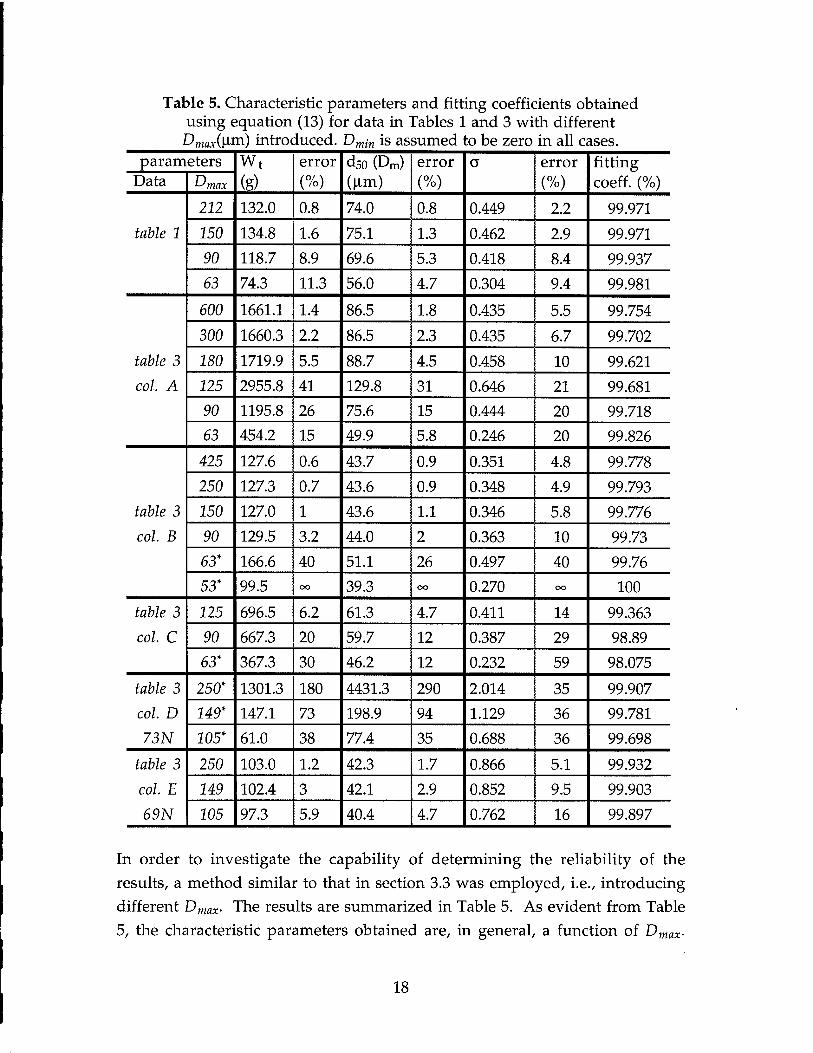
Table 5. Characteristic parameters and fitting coefficients obtained using equation (13) for data in Tables 1 and 3 with different Dmaxdua) introduced. Dmin is assumed to be zero in all cases.

parameters Wt

(g)

error

(%)

dso (Dm) (Jim)

error

(%)

a error

(%)

fitting Data L^max coeff. (%)

212 132.0 0.8 74.0 0.8 0.449 2.2 99.971

table 1 150 134.8 1.6 75.1 1.3 0.462 2.9 99.971

90 118.7 8.9 69.6 5.3 0.418 8.4 99.937

63 74.3 11.3 56.0 4.7 0.304 9.4 99.981

600 1661.1 1.4 86.5 1.8 0.435 5.5 99.754

300 1660.3 2.2 86.5 2.3 0.435 6.7 99.702

table 3 180 1719.9 5.5 88.7 4.5 0.458 10 99.621

col. A 125 2955.8 41 129.8 31 0.646 21 99.681

90 1195.8 26 75.6 15 0.444 20 99.718

63 454.2 15 49.9 5.8 0.246 20 99.826

425 127.6 0.6 43.7 0.9 0.351 4.8 99.778

250 127.3 0.7 43.6 0.9 0.348 4.9 99.793

table 3 150 127.0 1 43.6 1.1 0.346 5.8 99.776

col. B 90 129.5 3.2 44.0 2 0.363 10 99.73

63* 166.6 40 51.1 26 0.497 40 99.76

53* 99.5 oo 39.3 oo 0.270 oo 100

table 3 125 696.5 6.2 61.3 4.7 0.411 14 99.363

col. C 90 667.3 20 59.7 12 0.387 29 98.89

63* 367.3 30 46.2 12 0.232 59 98.075

table 3 250* 1301.3 180 4431.3 290 2.014 35 99.907

col. D 149* 147.1 73 198.9 94 1.129 36 99.781

73N 105* 61.0 38 77.4 35 0.688 36 99.698

table 3 250 103.0 1.2 42.3 1.7 0.866 5.1 99.932

col. E 149 102.4 3 42.1 2.9 0.852 9.5 99.903

69N 105 97.3 5.9 40.4 4.7 0.762 16 99.897

In order to investigate the capability of determining the reliability of the results, a method similar to that in section 3.3 was employed, i.e., introducing different Dmax. The results are summarized in Table 5. As evident from Table 5, the characteristic parameters obtained are, in general, a function of Dmax.

18

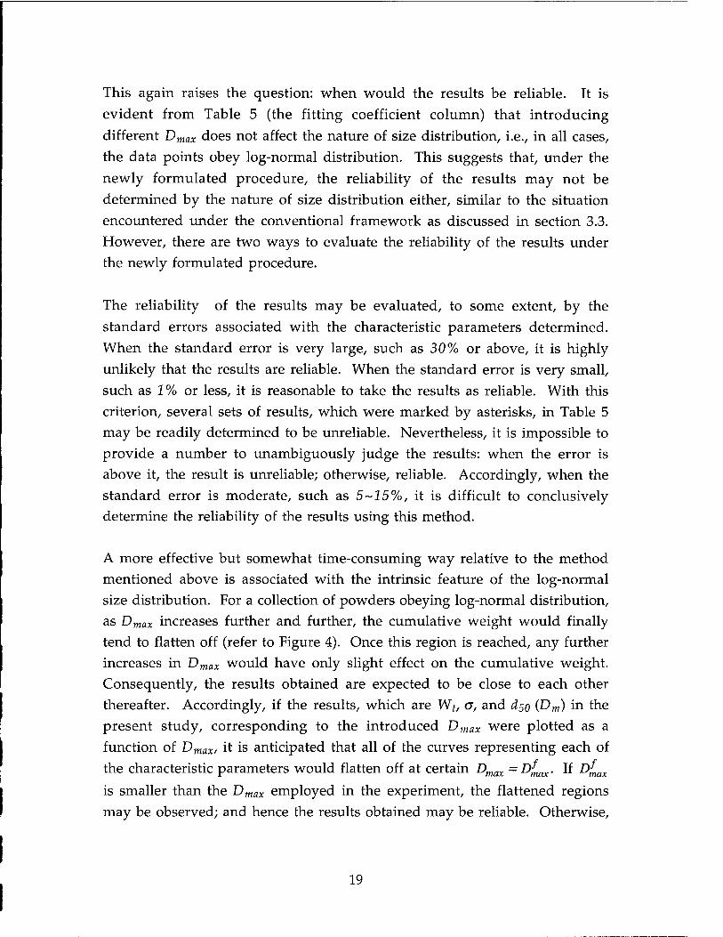
This again raises the question: when would the results be reliable. It is evident from Table 5 (the fitting coefficient column) that introducing different Dmax does not affect the nature of size distribution, i.e., in all cases, the data points obey log-normal distribution. This suggests that, under the newly formulated procedure, the reliability of the results may not be determined by the nature of size distribution either, similar to the situation encountered under the conventional framework as discussed in section 3.3. However, there are two ways to evaluate the reliability of the results under the newly formulated procedure.

The reliability of the results may be evaluated, to some extent, by the standard errors associated with the characteristic parameters determined. When the standard error is very large, such as 30% or above, it is highly unlikely that the results are reliable. When the standard error is very small, such as 2% or less, it is reasonable to take the results as reliable. With this criterion, several sets of results, which were marked by asterisks, in Table 5 may be readily determined to be unreliable. Nevertheless, it is impossible to provide a number to unambiguously judge the results: when the error is above it, the result is unreliable; otherwise, reliable. Accordingly, when the standard error is moderate, such as 5-15%, it is difficult to conclusively determine the reliability of the results using this method.

A more effective but somewhat time-consuming way relative to the method mentioned above is associated with the intrinsic feature of the log-normal size distribution. For a collection of powders obeying log-normal distribution, as Dmax increases further and further, the cumulative weight would finally tend to flatten off (refer to Figure 4). Once this region is reached, any further increases in Dmax would have only slight effect on the cumulative weight. Consequently, the results obtained are expected to be close to each other thereafter. Accordingly, if the results, which are Wt, o, and dso (Dm) in the present study, corresponding to the introduced Dmax were plotted as a function of Dmax, it is anticipated that all of the curves representing each of the characteristic parameters would flatten off at certain Dmax = D^. If D^

is smaller than the Dmax employed in the experiment, the flattened regions may be observed; and hence the results obtained may be reliable. Otherwise,

19

the flattened regions would be absent, and the results would be thought unreliable. With this criterion, the reliability of the results may be evaluated.

60 80 100 120 140 160 180 200 220

D (Jim)

700

50 100 150 200 250 300 350 400 450 D (urn)

max vr^

Figure 5. The characteristic parameters (normalized) obtained under different introduced Dmax for data in Table 1 (a), columns A (b), B (c), C (d), D (e), and E (f) of Table 3.

20

1.2

1.0

S 0.8 a

0.6

0.4 .

0.2 .

0.0 60

■W.

■d50 (Dm)

_i_L. ■ ■

70 80 90 D

100 (p.m)

110 120 130

100 120 140 160 180 200 220 240 260 D (Jim)

1.2

1.0

a o.8 s a BH 0.6

l04 e Z 0.2

0.0

■ wt

CD»)

■ ■ ■ ' ' ' ■ ■ ■ ■ '

100 120 140 160 180 200 220 240 260 D (llm) max v™ '

Figure 5 (continued). The characteristic parameters (normalized) obtained under different introduced Dmax for data in Table 1 (a), columns A (b), B (c), C (d), D (e), and E (f) of Table 3.

21

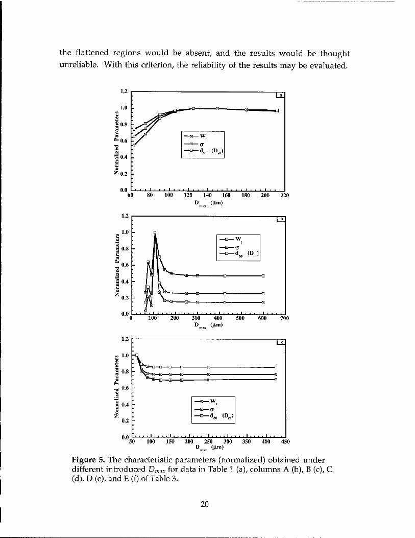
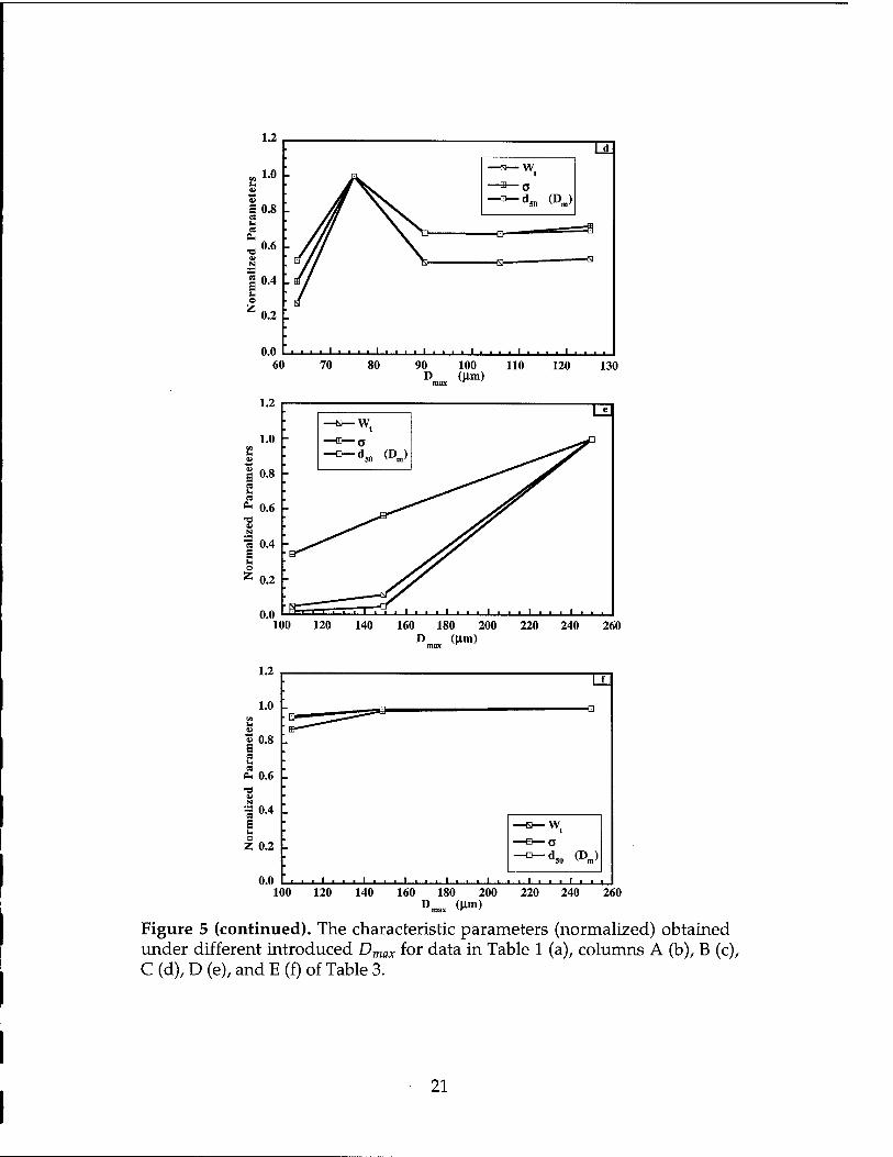
Figures 5(a) through (f) show the obtained results as a function of Dmax for the six sets of data under analysis. For the convenience of graphical representation, all of the results, for any given set of data, were normalized by their corresponding maximum magnitude. For example, the maximum

extracted total weight for the data in column B of Table 3 is 166.6 g, corresponding to an introduced Dmax of 63 \im. Accordingly, in Figure 5(c), all Wt values were normalized by 266.6 g. It is evident from Figure 5 that, except those in Figure 5(e), all of the curves exhibit a flattened out region as Dmax

increases. Moreover, for each specific set of data, the Dmax at which the curve begins to flatten is almost the same for all of the three parameters, Wt, a, and d-50 (Dm). For example, in Figure 5(c), all of the three parameters tend to be relatively insensitive to the change of Dmax after Dmax increases to 90 |im and beyond. The extended flattened regions in Figures 5(a)-(c) suggest that the data corresponding to these figures, which are the data in Table 1, columns A, and B of Table 3, respectively, are highly sufficient to yield reliable results. The limited flattened regions in Figures 5(d) and (f) implies that the results obtained with Dmax equal to that employed in experiment are almost reliable. In these cases, even though it is not mandatory, more data points, i.e., larger Dmax employed in the experiment, would be helpful to gain more confidence on the results. The absence of a flattened region in Figure 5(e) indicates that the data in column D of Table 3 are not sufficient to give any reliable results. Finally, it is of interest to note that before the flattened region was reached, the results may monotonously increase (Figure 5(a)) or decrease (Figure 5(c)), or vibrate back and forth (Figure 5(b)).

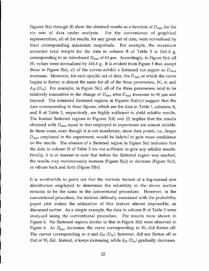
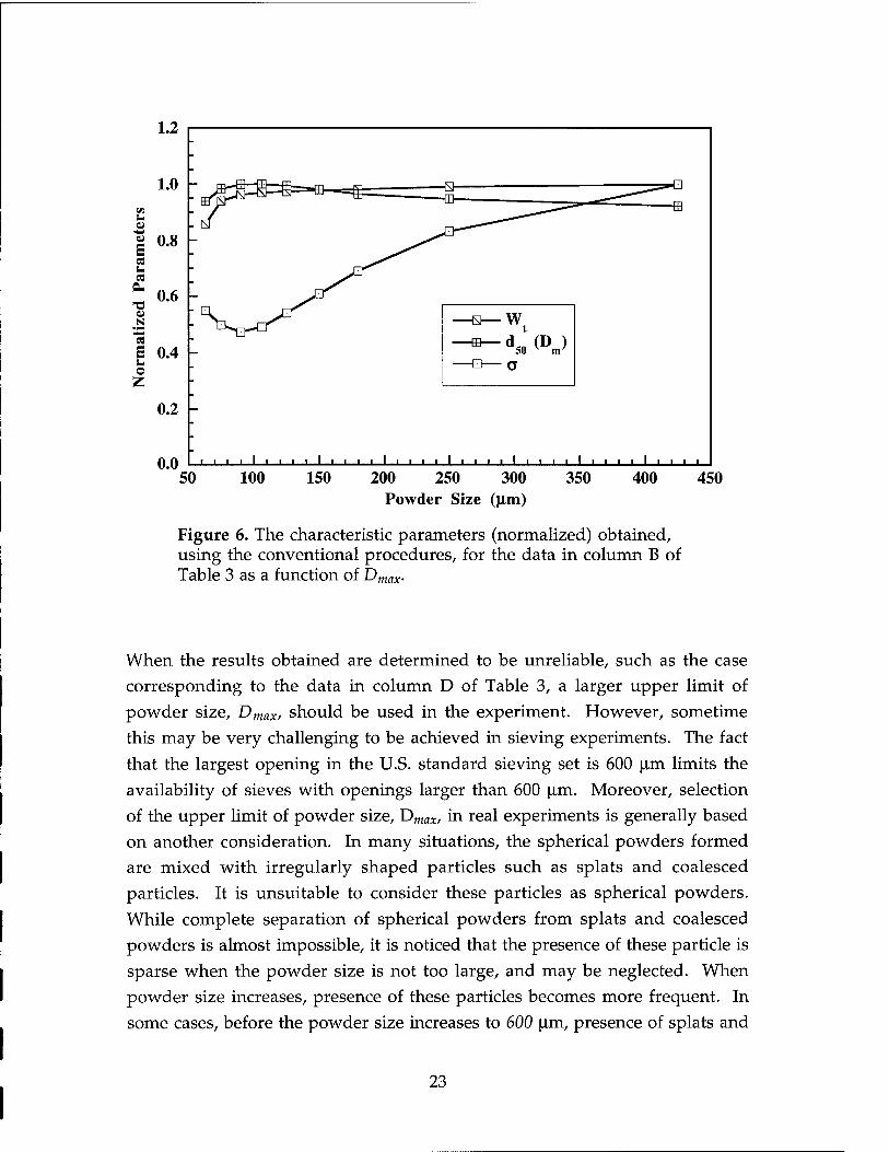
It is worthwhile to point out that the intrinsic feature of a log-normal size distribution employed to determine the reliability in the above section remains to be the same in the conventional procedure. However, in the conventional procedure, the intrinsic difficulty associated with the probability paper plot makes the utilization of this feature almost impossible, as discussed earlier. As a simple example, the data in column B of Table 3 were analyzed using the conventional procedure. The results were shown in Figure 6. No flattened regions similar to that in Figure 5(b) were observed in Figure 6. As Dmax increases, the curve corresponding to Wt did flatten off.

The curves corresponding to a and dso (Dm), however, did not flatten off as that of Wt did. Instead, a keeps increasing, while dso (Dm) gradually decreases.

22

09 U

es s- cd

OH

TJ 0) N

"c3 E S- o Z

1.2

1.0

0.8

0.6

0.4 -

0.2 -

0.0 50 100 200 250 300

Powder Size (um) 350 400 450

Figure 6. The characteristic parameters (normalized) obtained, using the conventional procedures, for the data in column B of Table 3 as a function of Dmax.

When the results obtained are determined to be unreliable, such as the case

corresponding to the data in column D of Table 3, a larger upper limit of

powder size, Dmax, should be used in the experiment. However, sometime

this may be very challenging to be achieved in sieving experiments. The fact

that the largest opening in the U.S. standard sieving set is 600 |xm limits the

availability of sieves with openings larger than 600 |i.m. Moreover, selection

of the upper limit of powder size, Dmax, in real experiments is generally based

on another consideration. In many situations, the spherical powders formed

are mixed with irregularly shaped particles such as splats and coalesced

particles. It is unsuitable to consider these particles as spherical powders.

While complete separation of spherical powders from splats and coalesced

powders is almost impossible, it is noticed that the presence of these particle is

sparse when the powder size is not too large, and may be neglected. When

powder size increases, presence of these particles becomes more frequent. In

some cases, before the powder size increases to 600 |im, presence of splats and

23

coalesced powders becomes so frequent that it can no longer be neglected compared with the total quantity of powders. Accordingly, a value smaller than 600 \im, for example 300 |im, is set to be the upper limit of powder size, below which presence of splats or coalesced powders can be neglected. Following this criterion of selection of Dmax, it may be unacceptable in some practical situations to raise Dmax to a value larger than the previously selected one, even though the newly selected value is smaller than 600 \im. In these cases, alternative existing characterization techniques, such as light -scattering, should be employed, or innovative techniques should be explored if meaningful results are anticipated.

100.0

•ä 90-ü|-

0123456789 10111213141516171819 20 2122 23 24 25 D p, Stokes Equivalent Diameters (jum)

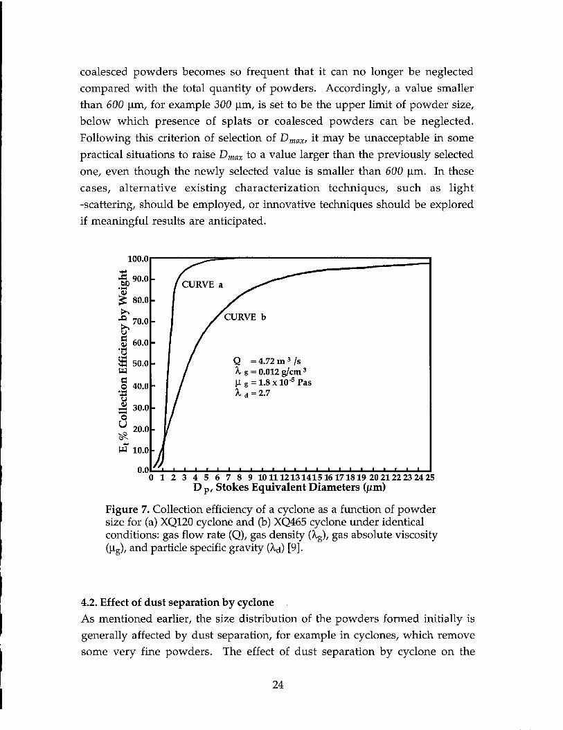
Figure 7. Collection efficiency of a cyclone as a function of powder size for (a) XQ120 cyclone and (b) XQ465 cyclone under identical conditions: gas flow rate (Q), gas density (kg), gas absolute viscosity (jig), and particle specific gravity (kd) [9].

4.2. Effect of dust separation by cyclone As mentioned earlier, the size distribution of the powders formed initially is generally affected by dust separation, for example in cyclones, which remove some very fine powders. The effect of dust separation by cyclone on the

24

distribution of the powders is somewhat different from that of the removal of

coarse powders. In the removal of coarse powders, the effect is discrete. For

example, if the powders are topped using a 425 urn sieve (35 mesh), powders

with size larger than 425 |j,m would be removed, while those with size

smaller than 425 urn would be left unaffected. In dust separation by cyclone,

the effect is continuous, as shown in Figure 7. Powders with powder size

smaller than 1 |xm would be almost completely removed. As the powder size

increases, the powders would be partially removed, and the percentage being

removed would gradually decreases to zero. This continuous feature greatly

complicates the problem. To make the problem tractable, a discrete removal,

similar to removal of coarse powders, will be assumed. This may be an

acceptable assumption if the collection efficiency curve is very steep, such as

in Figure 7.

4.2.1. Governing equations

When powders smaller than the lower limit of powder size, DmfM, are

removed, the experimentally obtained cumulative weight undersize, Wfnder(D), is nominal (refer to Figure 2). In this case, WE

nder(D) is the

cumulative weight of powders with size in the range from Dmin to D, rather

than from 0 to D. Therefore, Wunder(D) = Wu

Ender(D) + Wunder(Dmin) (15),

where Wunder(Dmin) is the cumulative weight under size Dmin. The

cumulative weight under size Dmin, Wunder(Dmin), may be further explicitly

expressed, in terms of Dmin, as follows:

/ J* Dmin-I« Dm

w„ 1 '"Dmin-'KDm

runder(Dmin) = Wt -j= j_ exp(-f2 /2)dt

= — WJnorm[-ln(^)] (16). 100 ' e Dm

,J

With equations (15) and (16), equations (10) and (13) would take the following

form

log D = log Dm + 0.434(7 ■ normllOO W^er(D) + Wmder(Dmin) ]

= logDm + 0.434G x

norm{100Wmder(D) +inorm[-ln(^-)]} (17), Wt a Dm

25

and

W*nder(D)=-^Wtinorm[±ln(-?-)]-Wunder(Dmin)

— Wtlinorml-lni—jJ-inorml-lni^^)]} (18), 100 a Dm o Dm

respectively.

In selection of the governing equation for curve fitting from equations (17)

and (18), arguments similar to those in section 4.1.2 apply here. Moreover,

equation (17) is much more complex than equation (18) in terms of computer

manipulation. Accordingly, equation (18) is uniquely selected as the

governing equation. Its usage in a computer is similar to that discussed in

section 4.1.3.

4.2.2. Evaluation of the effect ofDmin

The lower limit of powder size, Dmjn, is determined by design of the cyclone

[8]. It may range from 2 urn to 200 urn, depending on the details of the design

[8]. To illustrate its possible effect, Dmin=5,10, and 30 urn will be considered in

the present study.

The experimental data in Table 1 and in columns A, B, C, and E of Table 3

were analyzed using equation (18), with Dmjn in it set to be 5,10, and 30 um,

and Dmax equal to the ones employed in each experiment. The results, along

with those in Table 4 which correspond to the case with Dmjn=0 urn, were

summarized in Table 6. Data in column D of Table 3 were excluded from

further studies because of the incorrect selection of Dmax, as discussed earlier.

It is evident from Table 6 that the effect of Dm;M on the final results varies with

the magnitude of Dm;n itself, and with the powder collections under study.

For the data in Table 1 and in columns A, B, C of Table 3, Dmjn has little effect

on the final results when it is less than 10 um. As Dmz„ increases to 30 um,

distinct effects were observed for all of these data, with the most prominent

effect on the data in column B of Table 3. For the data in column E of Table 3,

Dmin has slight effect on the final results when it is 5 urn. As it increases to 20

urn, the effect becomes much more pronounced. When it is set to be 30 urn,

the results are completely different from those corresponding to Dmjn=0.

26

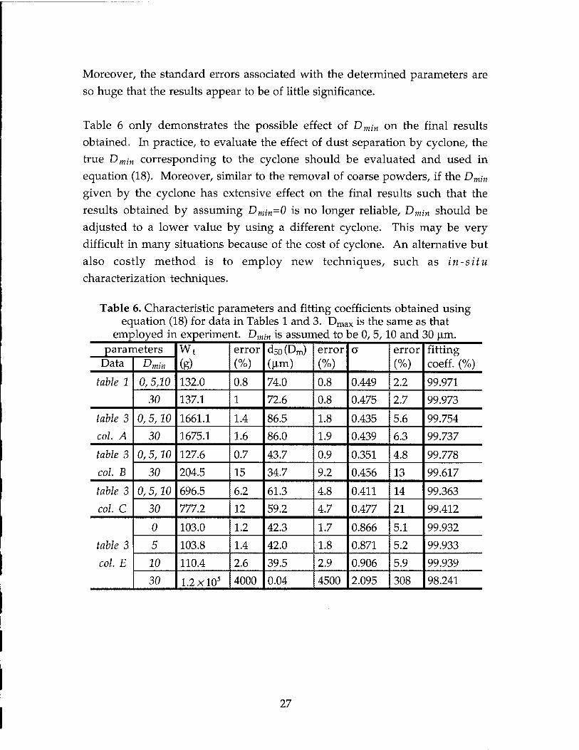
Moreover, the standard errors associated with the determined parameters are so huge that the results appear to be of little significance.

Table 6 only demonstrates the possible effect of Dmin on the final results obtained. In practice, to evaluate the effect of dust separation by cyclone, the true Dmin corresponding to the cyclone should be evaluated and used in equation (18). Moreover, similar to the removal of coarse powders, if the Dm;n

given by the cyclone has extensive effect on the final results such that the results obtained by assuming Dmin=0 is no longer reliable, DmjM should be adjusted to a lower value by using a different cyclone. This may be very difficult in many situations because of the cost of cyclone. An alternative but

also costly method is to employ new techniques, such as in-situ characterization techniques.

Table 6. Characteristic parameters and fitting coefficients obtained using equation (18) for data in Tables 1 and 3. Dmax is the same as that

employed in experiment. Dmjn is assumed to be 0, 5,10 and 30 )im. parameters Wt

(g)

error

(%)

dso (Dm) (|im)

error (%)

a error

(%)

fitting Data '-'min coeff. (%)

table 1 0,5,20 132.0 0.8 74.0 0.8 0.449 2.2 99.971

30 137.1 1 72.6 0.8 0.475 2.7 99.973

table 3 0,5,10 1661.1 1.4 86.5 1.8 0.435 5.6 99.754

col. A 30 1675.1 1.6 86.0 1.9 0.439 6.3 99.737

table 3 0,5,10 127.6 0.7 43.7 0.9 0.351 4.8 99.778

col. B 30 204.5 15 34.7 9.2 0.456 13 99.617

table 3 0,5,10 696.5 6.2 61.3 4.8 0.411 14 99.363

col. C 30 777.2 12 59.2 4.7 0.477 21 99.412

0 103.0 1.2 42.3 1.7 0.866 5.1 99.932

table 3 5 103.8 1.4 42.0 1.8 0.871 5.2 99.933

col. E 10 110.4 2.6 39.5 2.9 0.906 5.9 99.939

30 1.2 x10s 4000 0.04 4500 2.095 308 98.241

27

CHAPTER 5. SUMMARY

The procedure conventionally employed to interpret the experimental sieving data was examined. It was demonstrated that the conventional procedure is flawed from several standpoints. Along with several implicit, hard-to-be-justified, assumptions associated with it, the conventional graphical representation procedure also failed to address the reliability of its results. To resolve these problems, a new procedure was formulated. Application of the formulated procedure to several sets of sample sieving data reveals that it is capable of extracting the total weight of powders from experimental data, of determining the nature of size distribution, of characterizing the characteristic parameters, and simultaneously, of determining the reliability of its results.

28

REFERENCES

1. R. R. Irani and C. F. Callis, Particle Size: Measurement, Interpretation,

and Application, John Wiley & Sons, New York (1963).

2. T. Allen, Particle Size Measurement, Chapman and Hall, London (1981).

3. P. S. Grant, B. Cantor and L. Katgerman, Ada Metall. Mater. 41, 3109

(1993).

4. A. Jeffrey, Handbook of Mathematical Formulas and Integrals,

Academic Press, San Diego (1995).

5. F. Kottler, /. Franklin Inst. 250, 419 (1950).

6. R. R. Irani, /. Phys. Chem. 63, 1603 (1959).

7. C. Danial and F. S. Wood, Fitting Equations to Data, John Wiley & Sons, New York (1980).

8. O. Storch, Industrial Separators for Gas Cleaning, Elsevier, Amsterdam (1979).

9. Fisher-Klosterman Inc., Bulletin 218-C, "XQ Series High Performance Cyclones", (1980).

10. R. M. German, Powder Metallurgy Science, MPIF, Princeton, N.J. (1984).

11. M. L. Lau, B. Huang, R. J. Perez, S. R. Nutt and E. J. Lavernia, in Processing and Properties of Nanocrystalline Materials (Proc. Conf), p. 255, Cleveland, OH (1995).

12. R. J. Perez, B.-L. Huang, P. J. Crawford, A. A. Sharif and E. J. Lavernia, NanoStructured Materials 7, 47 (1996).

13. N. Yang, S. E. Guthrie, S. Ho and E. J. Lavernia, /. Mater. Synth. Proc. 4, 15 (1996).

14. R. J. Grandzol and J. A. Tallmadge, AIChE Journal 19, 1149 (1973).

29

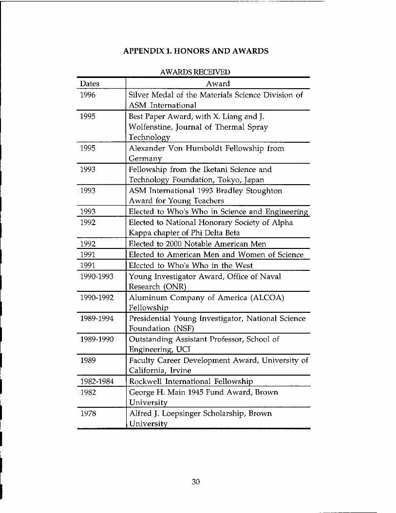
APPENDIX 1. HONORS AND AWARDS

AWARDS RECEIVED

Dates Award

1996 Silver Medal of the Materials Science Division of ASM International

1995 Best Paper Award, with X. Liang and J. Wolfenstine, Journal of Thermal Spray Technology

1995 Alexander Von Humboldt Fellowship from Germany

1993 Fellowship from the Iketani Science and Technology Foundation, Tokyo, Japan

1993 ASM International 1993 Bradley Stoughton Award for Young Teachers

1993 Elected to Who's Who in Science and Engineering 1992 Elected to National Honorary Society of Alpha

Kappa chapter of Phi Delta Beta

1992 Elected to 2000 Notable American Men 1991 Elected to American Men and Women of Science

1991 Elected to Who's Who in the West

1990-1993 Young Investigator Award, Office of Naval Research (ONR)

1990-1992 Aluminum Company of America (ALCOA) Fellowship

1989-1994 Presidential Young Investigator, National Science Foundation (NSF)

1989-1990 Outstanding Assistant Professor, School of Engineering, UCI

1989 Faculty Career Development Award, University of California, Irvine

1982-1984 Rockwell International Fellowship

1982 George H. Main 1945 Fund Award, Brown University

1978 Alfred J. Loepsinger Scholarship, Brown University

30

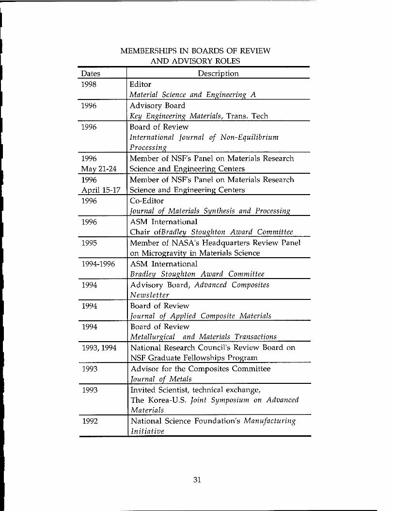
MEMBERSHIPS IN BOARDS OF REVIEW AND ADVISORY ROLES

Dates Description

1998 Editor Material Science and Engineering A

1996 Advisory Board Key Engineering Materials, Trans. Tech

1996 Board of Review International Journal of Non-Equilibrium Processing

1996 May 21-24

Member of NSF's Panel on Materials Research Science and Engineering Centers

1996 April 15-17

Member of NSF's Panel on Materials Research Science and Engineering Centers

1996 Co-Editor Journal of Materials Synthesis and Processing

1996 ASM International Chair oiBradley Stoughton Award Committee

1995 Member of NASA's Headquarters Review Panel on Microgravity in Materials Science

1994-1996 ASM International Bradley Stoughton Award Committee

1994 Advisory Board, Advanced Composites Newsletter

1994 Board of Review Journal of Applied Composite Materials

1994 Board of Review Metallurgical and Materials Transactions

1993,1994 National Research Council's Review Board on NSF Graduate Fellowships Program

1993 Advisor for the Composites Committee Journal of Metals

1993 Invited Scientist, technical exchange, The Korea-U.S. Joint Symposium on Advanced Materials

1992 National Science Foundation's Manufacturing Initiative

31

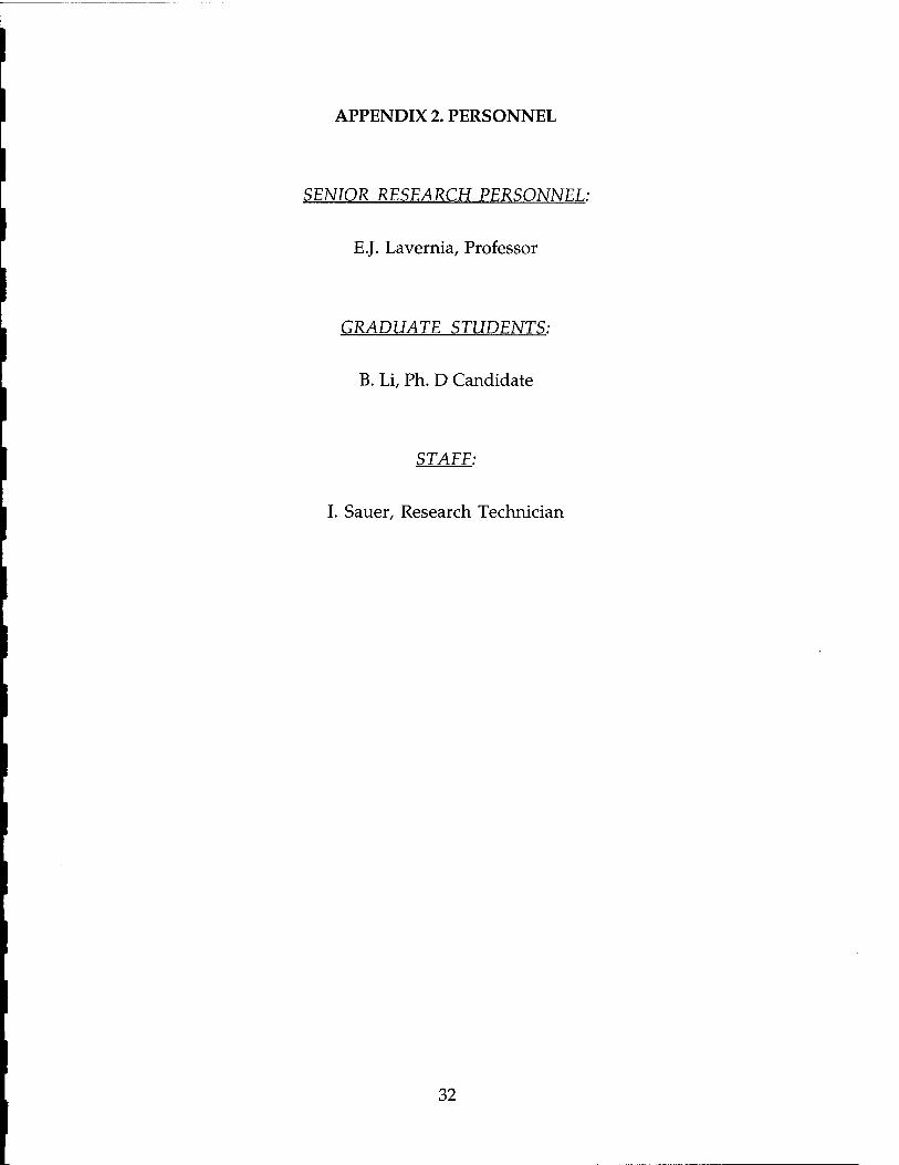
APPENDIX 2. PERSONNEL

SENIOR RESEARCH PERSONNEL:

E.J. Lavernia, Professor

GRADUATE STUDENTS:

B. Li, Ph. D Candidate

STAFF:

I. Sauer, Research Technician

32