Report 181

8/8/2019 Report 181

http://slidepdf.com/reader/full/report-181 1/27

I. INTRODUCTION

Most developing countries, facing persistent budget deficit and balance of

payment crisis, adopted Structural Adjustment Programme (SAP hereinafter) in

1980s. Under the programme there has been a general shift away from the

quantitative restrictions and price controls towards liberalisation and privatisation.

Has this policy package resulted in the desired results of improving the economic

conditions, structural imbalance and income distribution in Pakistan or not? This is

an important question. Such a question may be answered by simulation a priori or

actual trends against counter factual in the absence of such changes. A number of

empirical studies, in 1990’s, examined this question1 and showed that in most

countries the initial impact of the reforms was worsening growth rates and income

distribution. However, in the long run, some countries were able to improve theeconomic growth and income distribution while the others were worse off even in

the long run. In case of Pakistan, empirical studies suggest that distributional

impact of SAP is unevenly distributed among the population, hurting the most

vulnerable group the most.2 None of the studies, however, compared the results

with counter factual.

In late 80s and during 90s, Pakistan liberalised imports under SAP in

order to enhance the capacity utilisation of the domestic industry and

competitiveness of the commodity producing sectors. Before adjustment period,

Pakistan’s growth performance was satisfactory and income distribution

improved but in 1990s growth rate fell and a large proportion of population fell

below poverty lines as proportion of poor in population increased from 17.32

percent in 1987-88 to 32.6 percent in 1998-99. Given the situation of persistent budget and trade deficit and rising

poverty there is a need to explore, explicitly, the outcome of these policies,

particularly the policies having direct bearing on trade deficit, using an

appropriate quantitative framework.3 McGillivary et al. (1995) evaluated

1See for example, Kemal (1994), Amjad and Kemal (1997), Anwar (1998), Siddiqui and

Iqbal (1999), Iqbal and Siddiqui (1999), Bourguignon et al. (1991), Lambert et al. (1991), and

Robinson (1990). 2See Kemal (1994), Amjad and Kemal (1997), Anwar (1998), Siddiqui and Iqbal (1999)

and Iqbal and Siddiqui (1999). While White (1997), citing the case of African countries, has argued

that welfare indicators are expected to perform better in countries adopting adjustment policies than

those which do not.3

See for example MCHD (1999).

8/8/2019 Report 181


2

various methodologies used to assess the impact of SAP and concluded that

most appropriate method is econometric modelling. Because of the sensitivity of

domestic resource allocation to the developments of the external sector,

Computable General Equilibrium Models are very suitable for the analysis. In

SAM based CGE framework, a simulation exercise can help to determine the

impact of different policies and identify optimal policies leading to a better

outcome.4 For example changes in trade tax reforms (e.g., tariff reduction) affect

the pattern of sectoral demand, which can be well captured by the

disaggregation of production sector through CGE model which takes into

account the whole economy. The specific question to be explored in this study

is: whether trade liberalisation (tariff reduction) policies have improved income

distribution and reduced poverty in Pakistan or not?

This paper intends to explore functional and households personal

income distribution across four different income groups in both the urban and

rural areas. Siddiqui and Iqbal (1999), using Social Accounting framework,

come to the expected conclusion that poorer segment of population receives

higher proportion of income from wages and salaries whereas the rich class

receives highest share from capital income. The proportional change in the

returns to labour and to capital will determine the beneficiaries of the change

in policy. Another study by Iqbal and Siddiqui (1999b) shows that income

distribution, under fiscal adjustment, has worsened in urban areas and

improved in rural areas of Pakistan,5 while in reality, reverse has happened6.

In this paper three different simulation exercises are conducted to analyse the

impact of trade liberalisation policies on the performance of the economy as a

whole and on income accruing to households in different income groups from

different sources, which ultimately affects consumption pattern and welfare of

households.

Utilising the framework developed by Decaluwe et al. (1996), this

study explores the impact of tariff reduction on income distribution. For this

purpose the study by Siddiqui and Iqbal (1999) is extended in three directions.First, the households are disaggregated by four income categories in urban and

rural areas. Second, the Cobb-Douglas production framework is replaced by

Constant Elasticity of Substitution (CES) production function. Third, three

simulation exercises are conducted for analysing the impact of 40 percent, 60

percent and 80 percent reduction in tariff duty on industrial imports.

4For developing countries models, see Bourguignon et al. (1991), Lambert et al. (1991),

Robinson (1990). 5There are some limitations of SAM based analysis [For details see Shoven and Whalley

(1984) and Naqvi (1997)]. 6In depth analysis is needed to explore the reasons. Our future study “Impact of Fiscal

Adjustment on Income Distribution: A CGE-based Analysis” will be very helpful.

8/8/2019 Report 181


3

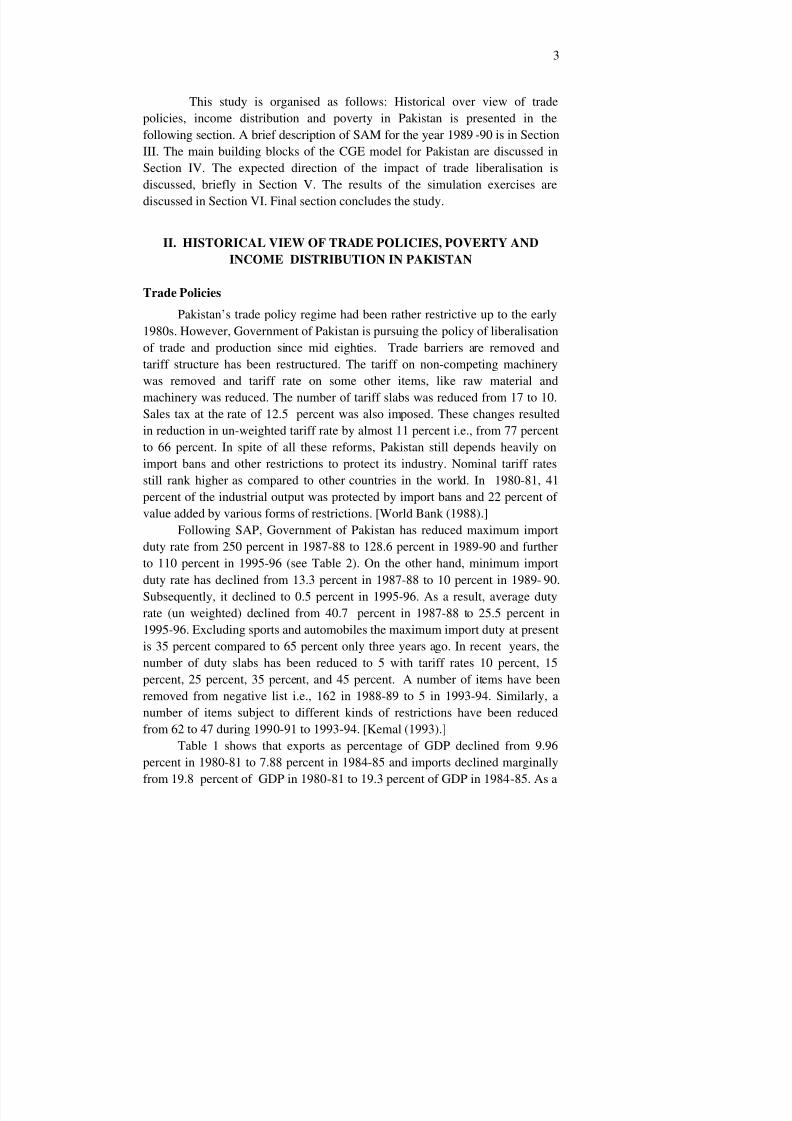
This study is organised as follows: Historical over view of trade

policies, income distribution and poverty in Pakistan is presented in the

following section. A brief description of SAM for the year 1989-90 is in Section

III. The main building blocks of the CGE model for Pakistan are discussed in

Section IV. The expected direction of the impact of trade liberalisation is

discussed, briefly in Section V. The results of the simulation exercises are

discussed in Section VI. Final section concludes the study.

II. HISTORICAL VIEW OF TRADE POLICIES, POVERTY AND

INCOME DISTRIBUTION IN PAKISTAN

Trade Policies

Pakistan’s trade policy regime had been rather restrictive up to the early

1980s. However, Government of Pakistan is pursuing the policy of liberalisation

of trade and production since mid eighties. Trade barriers are removed and

tariff structure has been restructured. The tariff on non-competing machinery

was removed and tariff rate on some other items, like raw material and

machinery was reduced. The number of tariff slabs was reduced from 17 to 10.

Sales tax at the rate of 12.5 percent was also imposed. These changes resulted

in reduction in un-weighted tariff rate by almost 11 percent i.e., from 77 percent

to 66 percent. In spite of all these reforms, Pakistan still depends heavily on

import bans and other restrictions to protect its industry. Nominal tariff rates

still rank higher as compared to other countries in the world. In 1980-81, 41

percent of the industrial output was protected by import bans and 22 percent of

value added by various forms of restrictions. [World Bank (1988).]

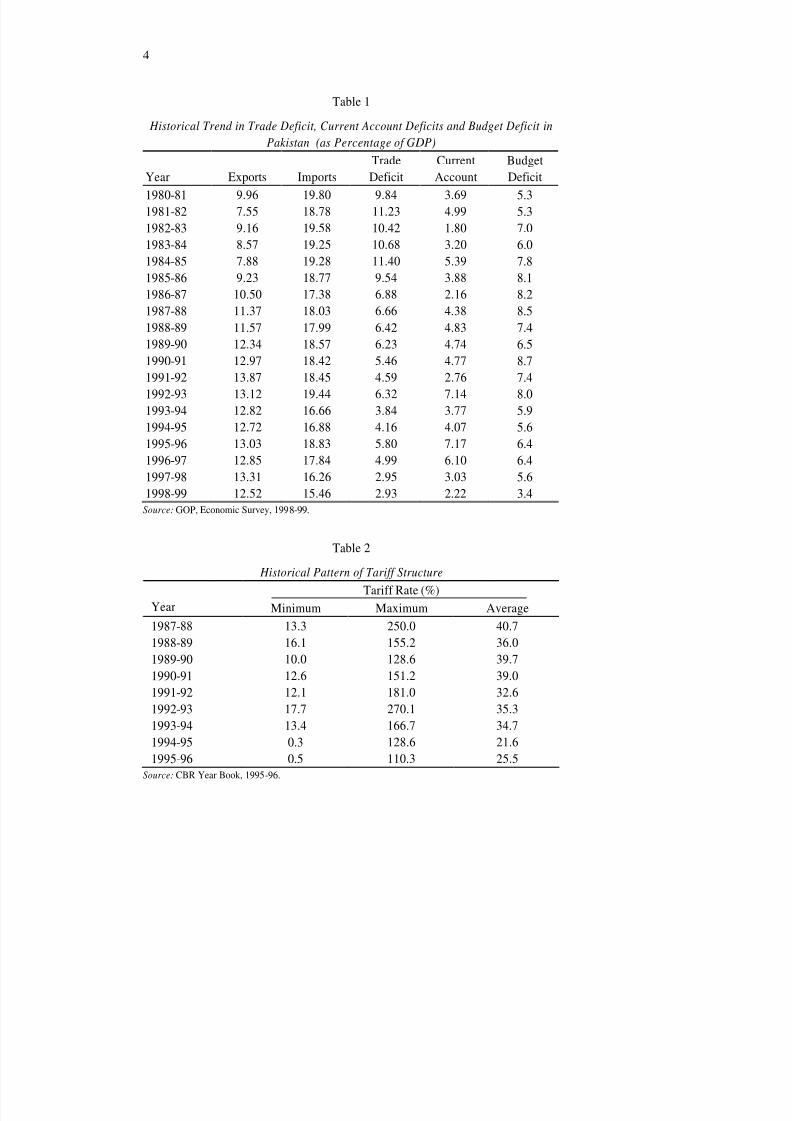
Following SAP, Government of Pakistan has reduced maximum import

duty rate from 250 percent in 1987-88 to 128.6 percent in 1989-90 and further

to 110 percent in 1995-96 (see Table 2). On the other hand, minimum import

duty rate has declined from 13.3 percent in 1987-88 to 10 percent in 1989- 90.

Subsequently, it declined to 0.5 percent in 1995-96. As a result, average duty

rate (un weighted) declined from 40.7 percent in 1987-88 to 25.5 percent in

1995-96. Excluding sports and automobiles the maximum import duty at present

is 35 percent compared to 65 percent only three years ago. In recent years, the

number of duty slabs has been reduced to 5 with tariff rates 10 percent, 15

percent, 25 percent, 35 percent, and 45 percent. A number of items have been

removed from negative list i.e., 162 in 1988-89 to 5 in 1993-94. Similarly, a

number of items subject to different kinds of restrictions have been reduced

from 62 to 47 during 1990-91 to 1993-94. [Kemal (1993).]

Table 1 shows that exports as percentage of GDP declined from 9.96

percent in 1980-81 to 7.88 percent in 1984-85 and imports declined marginally

from 19.8 percent of GDP in 1980-81 to 19.3 percent of GDP in 1984-85. As a

8/8/2019 Report 181


4

Table 1

Historical Trend in Trade Deficit, Current Account Deficits and Budget Deficit in

Pakistan (as Percentage of G DP)

Year Exports Imports

Trade

Deficit

Current

Account

Budget

Deficit

1980-81 9.96 19.80 9.84 3.69 5.3 1981-82 7.55 18.78 11.23 4.99 5.3

1982-83 9.16 19.58 10.42 1.80 7.0

1983-84 8.57 19.25 10.68 3.20 6.0

1984-85 7.88 19.28 11.40 5.39 7.8

1985-86 9.23 18.77 9.54 3.88 8.1

1986-87 10.50 17.38 6.88 2.16 8.2

1987-88 11.37 18.03 6.66 4.38 8.5

1988-89 11.57 17.99 6.42 4.83 7.4

1989-90 12.34 18.57 6.23 4.74 6.5

1990-91 12.97 18.42 5.46 4.77 8.7

1991-92 13.87 18.45 4.59 2.76 7.4

1992-93 13.12 19.44 6.32 7.14 8.0 1993-94 12.82 16.66 3.84 3.77 5.9

1994-95 12.72 16.88 4.16 4.07 5.6

1995-96 13.03 18.83 5.80 7.17 6.4

1996-97 12.85 17.84 4.99 6.10 6.4

1997-98 13.31 16.26 2.95 3.03 5.6

1998-99 12.52 15.46 2.93 2.22 3.4

Source: GOP, Economic Survey, 1998-99.

Table 2

Historical Pattern of Tariff Structure

Tariff Rate (%) Year Minimum Maximum Average

1987-88 13.3 250.0 40.7

1988-89 16.1 155.2 36.0

1989-90 10.0 128.6 39.7

1990-91 12.6 151.2 39.0

1991-92 12.1 181.0 32.6

1992-93 17.7 270.1 35.3

1993-94 13.4 166.7 34.7

1994-95 0.3 128.6 21.6

1995-96 0.5 110.3 25.5

Source: CBR Year Book, 1995-96.

8/8/2019 Report 181


5

result deficit in trade balance increased from 9.8 percent to 11.4 percent. During

1984-85 to 1987-88, exports share increased but imports share in GDP declined

resulting in improvement in trade deficit. During this period remittances had

declined which resulted in increase in current account deficit. During the 90’s,

despite fluctuations the share of exports in GDP has risen from 11.4 percent as

percentage of GDP in 1987-88 to 13.3 percent of GDP in 1997-98. However,

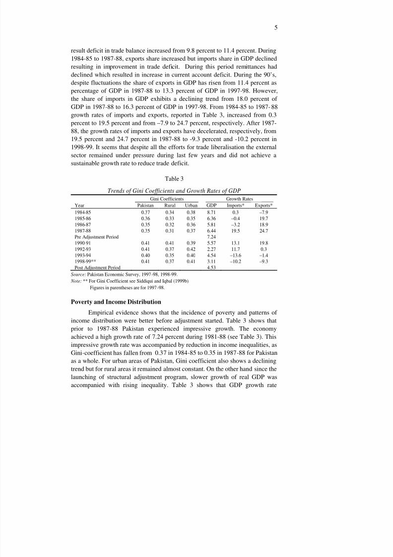
the share of imports in GDP exhibits a declining trend from 18.0 percent of GDP in 1987-88 to 16.3 percent of GDP in 1997-98. From 1984-85 to 1987- 88

growth rates of imports and exports, reported in Table 3, increased from 0.3

percent to 19.5 percent and from –7.9 to 24.7 percent, respectively. After 1987-

88, the growth rates of imports and exports have decelerated, respectively, from

19.5 percent and 24.7 percent in 1987-88 to -9.3 percent and -10.2 percent in

1998-99. It seems that despite all the efforts for trade liberalisation the external

sector remained under pressure during last few years and did not achieve a

sustainable growth rate to reduce trade deficit.

Table 3

Trends of Gini Coefficients and Growth Rates of GDP

Gini Coefficients Growth Rates

Year Pakistan Rural Urban GDP Imports* Exports*

1984-85 0.37 0.34 0.38 8.71 0.3 –7.9

1985-86 0.36 0.33 0.35 6.36 –0.4 19.7

1986-87 0.35 0.32 0.36 5.81 –3.2 18.9

1987-88 0.35 0.31 0.37 6.44 19.5 24.7

Pre Adjustment Period 7.24

1990-91 0.41 0.41 0.39 5.57 13.1 19.8

1992-93 0.41 0.37 0.42 2.27 11.7 0.3

1993-94 0.40 0.35 0.40 4.54 –13.6 –1.4

1998-99** 0.41 0.37 0.41 3.11 –10.2 –9.3

Post Adjustment Period 4.53

Source: Pakistan Economic Survey, 1997-98, 1998-99.

Note: ** For Gini Coefficient see Siddiqui and Iqbal (1999b).

Figures in parentheses are for 1997-98.

Poverty and Income Distribution

Empirical evidence shows that the incidence of poverty and patterns of

income distribution were better before adjustment started. Table 3 shows that

prior to 1987-88 Pakistan experienced impressive growth. The economy

achieved a high growth rate of 7.24 percent during 1981-88 (see Table 3). This

impressive growth rate was accompanied by reduction in income inequalities, as

Gini-coefficient has fallen from 0.37 in 1984-85 to 0.35 in 1987-88 for Pakistan

as a whole. For urban areas of Pakistan, Gini coefficient also shows a declining

trend but for rural areas it remained almost constant. On the other hand since the

launching of structural adjustment program, slower growth of real GDP was

accompanied with rising inequality. Table 3 shows that GDP growth rate

8/8/2019 Report 181


6

declined from 7.24 percent during pre adjustment period (1980-81 to 1987-88)

to 4.53 percent in post adjustment period (1988-89 to 1998-99). Gini

coefficients rose to 0.41 for Pakistan as a whole and to 0.37 and 0.42 for rural

and urban areas, respectively. Gini coefficients improved marginally (i.e., 0.40)

in 1993-94 when GDP growth rate rose to 4.54 percent. Gini coefficient for

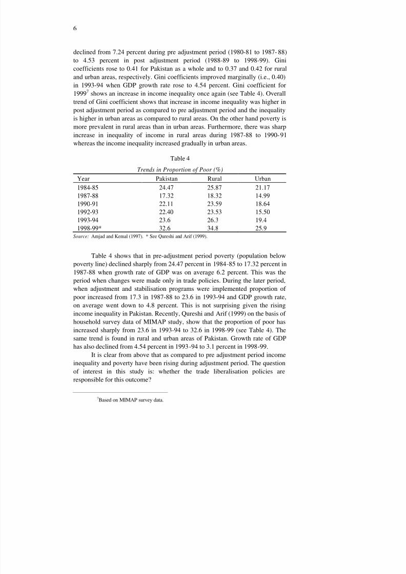
19997 shows an increase in income inequality once again (see Table 4). Overall

trend of Gini coefficient shows that increase in income inequality was higher inpost adjustment period as compared to pre adjustment period and the inequality

is higher in urban areas as compared to rural areas. On the other hand poverty is

more prevalent in rural areas than in urban areas. Furthermore, there was sharp

increase in inequality of income in rural areas during 1987-88 to 1990-91

whereas the income inequality increased gradually in urban areas.

Table 4

Trends in Proportion of Poor (%)

Year Pakistan Rural Urban

1984-85 24.47 25.87 21.17

1987-88 17.32 18.32 14.99

1990-91 22.11 23.59 18.64

1992-93 22.40 23.53 15.50

1993-94 23.6 26.3 19.4

1998-99* 32.6 34.8 25.9

Source: Amjad and Kemal (1997). * See Qureshi and Arif (1999).

Table 4 shows that in pre-adjustment period poverty (population below

poverty line) declined sharply from 24.47 percent in 1984-85 to 17.32 percent in

1987-88 when growth rate of GDP was on average 6.2 percent. This was the

period when changes were made only in trade policies. During the later period,

when adjustment and stabilisation programs were implemented proportion of

poor increased from 17.3 in 1987-88 to 23.6 in 1993-94 and GDP growth rate,

on average went down to 4.8 percent. This is not surprising given the rising

income inequality in Pakistan. Recently, Qureshi and Arif (1999) on the basis of

household survey data of MIMAP study, show that the proportion of poor has

increased sharply from 23.6 in 1993-94 to 32.6 in 1998-99 (see Table 4). The

same trend is found in rural and urban areas of Pakistan. Growth rate of GDP

has also declined from 4.54 percent in 1993-94 to 3.1 percent in 1998-99.

It is clear from above that as compared to pre adjustment period income

inequality and poverty have been rising during adjustment period. The question

of interest in this study is: whether the trade liberalisation policies are

responsible for this outcome?

7

Based on MIMAP survey data.

8/8/2019 Report 181


7

III. STRUCTURE OF SAM 1989-90 FOR PAKISTAN Every economy wide model, particularly CGE model, requires a

consistent data base. For this paper data arranged in Social Accounting

Matrix (SAM) framework provides the best consistent data set. The latest

SAM for the year 1989-90 is given in Siddiqui and Iqbal (1999) [see

Appendix II]. It presents a comprehensive picture of the whole economy. Itdisaggregates production activities into five sectors; agriculture, Industry,

education, health and other. These activities are then classified as traded

goods i.e., agriculture, industry, health and other and non-traded goods i.e.,

education. The factors of production are disaggregated into labour and

capital. The institutions are identified as households, firms, government and

rest of the world.8 In accordance with the orientation of analytical interest

and policy problems related with the field of distribution of income and

consumption, classifications in the SAM-1989-90 (in the present form)

highlights the income receipt pattern of households from different sources

and their uses on different items.

In this paper, as mentioned earlier, household sector is disaggregated by

region, rural and urban areas of Pakistan. In each region households are

categorised by four income groups: upto Rs 1500, Rs 1501-3000, 3001-5000,

and 5001 and above. The production sector is disaggregated by traded and non-

traded goods. This disaggregation allows to capture the effects of policy

changes on sectoral demands and supplies. The mechanisms by which policy

changes affect the distribution of income are as follows:

(a) Changes in factor rewards directly affecting household income

distribution.

(b) Changes in relative production prices affecting households’ real

income as basket of consumption goods differs by income group.

Selection of macroeconomic closure rule (which is how adjustmenttakes place) and institutional characteristics (assumptions about the working of

markets) determine the distributional outcome of policy change.9 The changes in

relative prices due to reduction in tariff will affect resource allocation, income

distribution and poverty alleviation. Since the outcome of policy change will

8We have distinguished household group in our earlier study [Siddiqui and Iqbal (1999)] into four

income groups for rural and urban areas of Pakistan separately. This disaggregation is carried out to

illustrate how the SAM framework and the related CGE model can combine the macro economic features

with microeconomic issues. Although disaggregation of the household sector is important to see the impact

on income distribution. But in Siddiqui and Iqbal (1999a), aggregate household sector was included. 9The simulation exercise shows how important closure rules and institutional settings are

to the distributive consequences of a shock.

8/8/2019 Report 181


8

vary with closure rule and institutional characteristics, the selection of

adjustment policy is very critical.

The present CGE model is built on the following assumptions:

(1) Primary factor supplies are exogenous to the model.

(2) Capital is immobile across the sector. Supply of capital stock is fixed

and it is sector specific. Change in demand for capital will changethe price of capital not the allocation.

(3) Labour is assumed to be mobile among the different production

activities. Wage rate is determined by labour demand equal to labour

supply.

(4) World prices of imports and exports are given.

(5) Government consumption and its transfers to households and firms

are also exogenous.

Closure: Since the economy has no impact on international markets, the

world prices of imports and exports are exogenous to the model. The current

account balance and the nominal exchange rate are also exogenous to the model.

The predetermined foreign saving has to equal to the import surplus.

Difference in assumptions and closure rule play a very important role inmarket adjustment mechanism. Adjustment to external shock through price

change, devaluation or fiscal retrenchment can be different for an economy with

different degree of financial and trade liberalisation. Simulation exercises show

that assumptions about the macro economic closure and behavioural parameters

matter a great deal in determining the productive and distributive effects of a

shock and a country’s adjustment to that shock. These exercises also show the

channels through which a country captures the effects of alternative adjustment

packages on income distribution. For example, resistance to wage cut and to

profit cut also has strong implications for the income distribution. Poverty is

likely to increase when there is resistance because the economy is not operating

at full capacity level. Changes in trade tax reforms (tariff) affect the pattern of

sectoral demand, which can be well captured by the disaggregation of production sector through CGE model.

IV. COMPUTABLE GENERAL EQUILIBRIUM MODEL

FOR PAKISTAN

Basic framework of the model is from Decaluwe et al. (1996). This neo-

classical framework contains six blocks with more than two hundred equations.

Exchange rate acts as numeraire. Its value is set equal to one. Mathematical

equations of the model, specification of variables and symbols are given in

Appendix I. The theoretical background of the equations in each block of CGE

model is discussed below:

8/8/2019 Report 181


9

1. Production Sector: Domestic production is disaggregated into five

sectors, viz., agriculture, industry, other, health and education. Like most

empirical studies, we have assumed a technology in which gross output has

separable production function for value added and intermediate consumption

with CES production functions for value added and Leontief technology

between intermediate and value added and also within intermediates are

assumed. Equations for gross output, value added (specified as a function of

labour (L) and capital (K)) and intermediate demand (aggregate as well as

disaggregated) are specified in Equations 1 to 4.

2. Factor Demand: Assuming perfect competition and market clearing,

labour demand function for ith sector is derived from CES production function.

Capital is sector specific and it is assumed to be given in the short run. Labour

demand is specified in Equation 5. While price of capital is determined by

equation 30 in price block. Changes in factor prices play important role in

explaining the issue of functional income distribution.

3. Foreign Trade Sector: In this sector, the model has separate

equations for exports and imports. We have assumed that domestic sales and

exports with the same sectoral classification represent goods of different

qualities. Constant Elasticity of Transformation CET function describes the

possible shift of sectoral production between domestic and external markets.

For import function, we assume that domestically produced goods sold in the

domestic market are imperfect substitute of imports (Armington assumption).

Constant Elasticity of Substitution (CES) import aggregation function presents

demand for composite goods (imported and domestically produced goods). In

addition to Equations 6 and Equation 7 for export transformation and import

aggregation, profit maximisation/cost minimisation gives desired exports and

imports ratios as a function of relative prices (domestic to foreign prices). (see

Equation 8 and Equation 9, respectively).

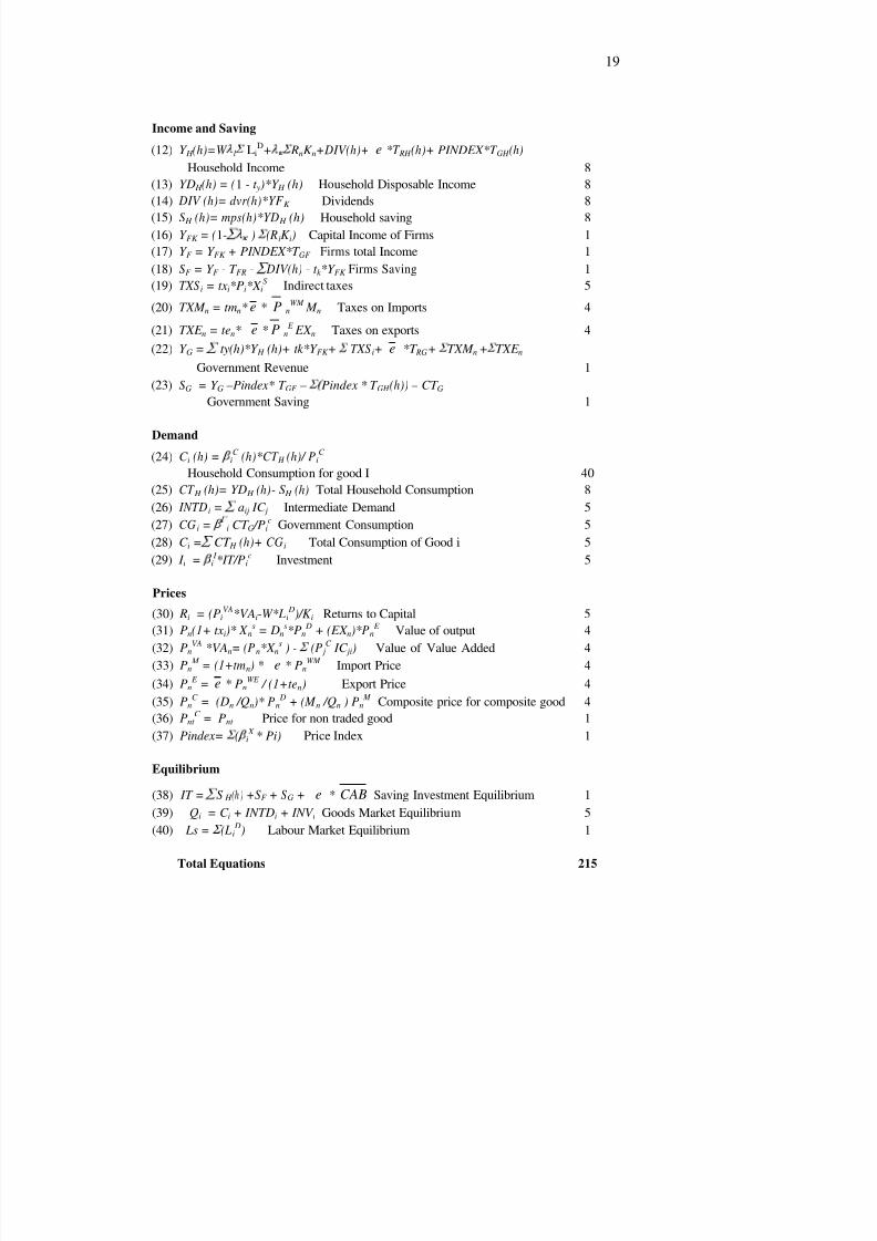
4. Income, Saving and Consumption: Institutions receive income from

different sources. The endowment of primary factors and their rental valuesdetermine the institutional income from factors of production. All incomes of

institutions is used for consumption and rest is saved. Relevant equations are

given in income and saving block of the model.

5. Households: In this study, we analyse functional distribution of

income among different income groups and institutions. All wage income

accrues to households and the households also receive share of capital income

from total capital income from different activities. They also receive income

from firms as dividends, transfers from government as social security benefits,

and transfers from the rest of the world. Equation 12, representing hth

household represents total income of households from above mentioned sources.

Dividends for the hth household are determined by Equation 14. Transfers from

8/8/2019 Report 181


10

the government and from the rest of the world are assumed to be exogenous.

Households pay taxes to government. Subtracting taxes from the total income

we get disposable income of households. Different income groups spend this

income on different commodities. Consumption of ith commodity by jth

households and total household consumption are defined by Equation 24 and

Equation 25, respectively. These equations describe how different goods are

consumed by households in different income groups. It is defined with fixed

value share of ith good. The sum of ic, is equal to 1. In addition, savings of hth

household is defined in Equation 15.

6. Firms: Firms receive income from operating surplus and transfers

from government. Equation 17 presents firm’s total income. Income from

capital (retained profit) is presented in Equation 16. Transfers from the

government are given exogenously. Its expenditure includes tax payments to the

government, dividends to hth households, and transfers to the rest of the world.

While residual is saved.

7. Government: Third institution i.e., government, receives income from

the following sources, i.e., direct taxes (income tax from households, corporate

taxes from firms), indirect taxes (from production sector), import duties (tariff),export duties(subsidies), and transfers from the rest of the world. Total

government revenue is given by Equation 22. Equations for indirect taxes, taxes

from imports and from exports are presented in Equations 19, 20, and 21,

respectively. Government total current expenditure is given in value.

Government total expenditure on ith commodity is fixed share calculated

through Equation 27. Government saving is calculated as a residual after

subtracting consumption expenditure from total revenue.

Total consumption expenditure on ith good is the sum of expenditure by

different household groups and by government on good i. In addition to

consumption expenditure, there is a demand for good i for the investment

purposes. Equation 29 converts aggregate investment into demand forinvestment good by sector of origin. I is gross fixed capital formation in

commodity i, Iij is fixed value share and its sum is equal to one. Gross saving

from different household groups, firms, government and rest of the world serve

as source of funding for gross investment.

8. Prices: Block 5 of the model presents different prices associated

with each tradable good, as price of aggregate output, price of composite

goods, price of domestic sale, domestic price of imports, domestic price of

exports, world price of imports, and world price of exports. World prices of

exports and imports are exogenously determined. All prices are defined in

Equations 30 through 36. Over all price index i.e., GDP deflator is presented

in Equation 37.

8/8/2019 Report 181


11

9. Equilibrium: Final block presents saving-investment equilibrium, goods

market equilibrium, and labour market equilibrium by Equations 38, 39, and 40,

respectively. Model is closed in Current Account Balance equation. Nominal

exchange rate is numerair. Real exchange rate is implicit in the model calculated as

follows.

er = e * (P

w

/ Pd )

V. THEORETICAL FRAMEWORK: IMPACT OF TRADE

LIBERALISATION ON INCOME DISTRIBUTION

Changes in prices play crucial role in resource allocation, income

distribution and poverty Alleviation. Changes in relative price structure, results

from tariff reduction, affects production incentives, consumption and other

economic indicators in an economy. Impact of tariff reduction on economy

depends on the extent to which the imposition of tariff reduction affects the

price of goods produced domestically. If these goods are substitutes to imported

goods, then reduction in tariff leading to lower import price will reduce demand

for domestically produced goods and increase demand for imported goods.

Reduced demand causes decline in prices of domestically produced goods aswell. Clearly the impact of these policies will depend on whether the imported

goods are complements or substitutes to domestically produced goods and on

the elasticity of supply of the product. Higher elasticity of supply requires

smaller adjustment in domestic prices necessary to bring back equilibrium in the

market. Furthermore, analysis of the impact of the changes in incentives and

resource allocation, in response to price changes, is very important as they

ultimately affect real income and welfare in the country.

There are three channels that affect income distribution in response to

adoption of structural adjustment policies [Bourguignon et al. (1991)]. Firstly,

changes in factor rewards directly affect households’ income.10 Secondly, changes

in relative product prices affect households’ real income differently because

consumption expenditure is specified at the household level. If we assume similarpreference function for all consumers in the economy then we can compare the

aggregate consumption with the consumption in the base line solution. If more of

every single commodity is consumed after policy shock that indicates improvement.

Thirdly, capital gains and losses affect households’ wealth distribution can not be

captured through this model. In this paper, we concentrate on the effects of tariff

rationalisation on income distribution among households in urban and rural areas.

We are utilising the multi-sector multi-factor CGE model in which distributional

10Generally poor households supply labour services and receive highest share of their income

from wages and salaries, as shown in Siddiqui and Iqbal (1999). While rich class receive higher percentage

of their income from capital. These channels affect income distribution.

8/8/2019 Report 181


12

shifts occur mostly through changes in relative prices, proposed by Decaluweet al.

(1996) to analyse the situation (see Appendix 1).

VI. COMPARISON OF BASELINE SOLUTION WITH

SIMULATION RESULTS

This section discusses the impact of reduction in tariff rate on industrial

imports on the macro aggregates in general and on income distribution and

consumption of different income groups in particular. Model is simulated by

reducing tariff rate on industrial imports by 40 percent, 60 percent, and 80

percent. The results of simulations are reported in Table 5.

The impact of tariff rate reduction depends on the interaction between the

domestic economy and the foreign trade sector. The first impact of reduction in

tariff rate is to lower price of industrial imports. This change in price affects the

input use in the economy. Consequently, production, income distribution,

consumption and saving change. We focus on the results of the third simulation,

i.e., 80 percent reduction in tariff rate of industrial imports.

The immediate impact of tariff reduction by 80 percent on industrial

imports is to lower import price of industrial imports by 16.37 percent. The

reduction in import price leads to decline in domestic price of industrial goods.The resulting decline in domestic industrial goods prices leads to decline in

supply of industrial products by 0.58 percent, and releases labour from

industrial production. The results show that labour demand in industrial sector

declined by 1.9 percent. The released labour is absorbed in other sectors.

Demand for labour increases in agriculture, health and education sector by 1.21

percent, 3.52 percent and 3.16 percent, respectively. While decline in non traded

sector is marginal. On the other hand demand for capital in agriculture, industry

and others sectors declines but increases in health and education. Since capital is

sector specific, the change in demand of capital affects prices in these sectors.

The results show that the net impact of change in price of factor of production

has resulted in change in share of labour and capital in GDP. However, this

change is very little as the share of labour and capital changes from 0.28 and0.72 to 0.27 and 0.73, respectively (see Table 6). This implies that benefits of

reduction in tariff rate on industrial imports are a little high for rich people

whose highest share of income comes from capital.11 Thus reduction in tariff

rate on industrial imports increases the income gap between rich and poor.

The results also show that contribution of different sectors to GDP has

also changed with the change in factors’ demand. The contribution of

agriculture, health, and education to GDP has increased after the tariff

adjustment, and share of industry and others sector has declined (See Table 7).

But the change is very small.

11

See Siddiqui and Iqbal (1999) for detail.

8/8/2019 Report 181


13

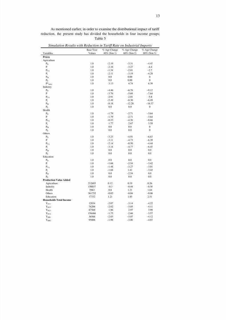
As mentioned earlier, in order to examine the distributional impact of tariff

reduction, the present study has divided the households in four income groups;

Table 5

Simulation Results with Reduction in Tariff Rate on Industrial Imports

Variables

Base Year

Values

%-Age Change

40% (Sim 1)

%-Age Change

60% (Sim 2)

%-Age Change

80% (Sim 3)

Prices

Agriculture

PD 1.0 –2.19 –3.31 –4.45

P 1.0 –2.16 –3.27 –4.4

PVA 1.0 –1.34 –2.01 –2.7

Pc 1.0 –2.11 –3.19 –4.29

PM 1.0 0.0 0.00 0

PE 1.0 0.0 0.00 0

P*index 1.0 –3.13 –4.74 –6.39

Industry

PD 1.0 –4.46 –6.76 –9.12

P 1.0 –3.76 –5.69 –7.64

PVA 1.0 –2.91 –2.01 –5.8

Pc 1.0 –5.49 –8.30 –6.49

PM 1.0 –8.18 –12.28 –16.37

PE 1.0 0.0 0.0 0

Health

PD 1.0 –1.79 –2.71 –3.64

P 1.0 –1.79 –2.71 –3.64

PVA 1.0 –0.33 –4.36 –0.66

Pc 1.0 –1.77 –2.67 –3.59

PM 1.0 0.0 0.0 0

PE 1.0 0.0 0.0 0

Others

PD 1.0 –3.23 –4.91 –6.63

P 1.0 –3.11 –4.73 –6.39

PVA 1.0 –2.14 –0.50 –4.44

Pc 1.0 –3.14 –4.77 –6.45

PM 1.0 0.0 0.0 0.0

PE 1.0 0.0 0.0 0.0

Education

PD 1.0 0.0 0.0 0.0

P 1.0 –1.68 –2.54 –3.42

PVA

1.0 –1.48 –3.27 –3.01

Pc 1.0 –1.68 1.41 –3.42

PM 1.0 0.0 –2.54 0.0

PE 1.0 0.0 0.0 0.0

Production Value Added

Agriculture 212693 0.12 0.19 0.26

Industry 150037 –0.3 –0.44 –0.58

Health 5963 0.8 1.21 1.64

Others 361752 –0.02 –0.04 –0.06

Education 17332 1.21 1.85 2.51

Households Total Income

YHU1 12034 –2.07 –3.14 –4.22

YHU2 76206 –2.02 –3.05 –4.11

YHU3 87569 –1.96 –2.97 –3.99

YHU4 154466 –1.75 –2.66 –3.57

YHR1 36566 –2.03 –3.07 –4.12

YHR2 95806 –1.98 –3.00 –4.03

8/8/2019 Report 181


14

YHR3 92099 –1.92 –2.91 –3.92

YHR4 130794 –1.91 –2.89 –3.89

Continued —

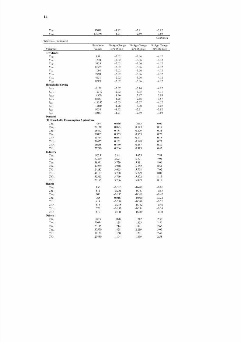
Table 5—(Continued )

Variables

Base Year

Values

%-Age Change

40% (Sim 1)

%-Age Change

60% (Sim 2)

%-Age Change

80% (Sim 3)

Dividends

YHU1 159 –2.02 –3.06 –4.12

YHU2 1540 –2.02 –3.06 –4.12 YHU3 5125 –2.02 –3.06 –4.12

YHU4 14569 –2.02 –3.06 –4.12

YHr1 1094 –2.02 –3.06 –4.12

YHr2 2790 –2.02 –3.06 –4.12

YHr3 4631 –2.02 –3.06 –4.12

YHr4 18968 –2.02 –3.06 –4.12

Households Saving

SHU1 –9159 –2.07 –3.14 –4.22

SHU2 –12312 –2.02 –3.05 –4.11

SHU3 –4300 –1.96 –2.97 –3.99

SHU4 40883 –1.75 –2.66 –3.57

SHr1 –18355 –2.03 –3.07 –4.12

SHr2 –12605 –1.98 –3.00 –4.03

SHr3 9638 –1.92 –2.91 –3.92

SHr4 60053 –1.91 –2.89 –3.89

Demand

(1) Households Consumption Agriculture Chu1 7097 0.036 1.053 0.07

Chu2 29128 0.095 0.143 0.19

Chu3 28472 0.151 0.229 0.31

Chu4 30005 0.363 0.553 0.75

CHr1 19764 0.087 0.131 0.18

CHr2 38457 0.131 0.198 0.27

CHr3 28685 0.189 0.287 0.39

CHr4 22290 0.206 0.313 0.42

Industry

Chu1 9025 3.61 5.625 7.81

Chu2 37479 3.671 5.721 7.94

Chu3 38391 3.729 5.811 8.06

Chu4 42239 3.948 6.152 8.54

CHr1 24282 3.663 5.708 7.92

CHr2 48187 3.708 5.779 8.02

CHr3 35363 3.769 5.872 8.15

CHr4 29195 3.786 5.899 8.19 Health

Chu1 150 –0.310 –0.477 –0.65

Chu2 611 –0.251 –0.387 –0.53

Chu3 600 –0.195 –0.302 –0.42

Chu4 765 0.016 –0.020 0.022

CHr1 419 –0.259 –0.399 –0.55

CHr2 818 –0.215 –0.332 –0.46

CHr3 576 –0.157 –0.244 –0.34

CHr4 610 –0.141 –0.219 –0.30

Others

Chu1 4775 1.098 1.712 2.38

Chu2 20634 1.158 1.803 2.50

Chu3 23115 1.214 1.891 2.62

Chu4 37570 1.428 2.219 3.07

CHr1 10152 1.150 1.791 2.48

CHr2 20450 1.194 1.859 2.58

8/8/2019 Report 181


15

CHr3 17309 1.253 1.949 2.70

CHr4 95 1.269 1.975 2.74

Continued —

Table 5—(Continued )

Education

Chu1 95 –0.403 –0.615 –0.83

Chu2 523 –0.344 –0.525 –0.71

Chu3 861 –0.288 –0.440 –0.60

Chu4 1882 –0.077 –0.119 –0.16 CHr1 118 –0.352 –0.537 –0.73

CHr2 405 –0.308 –0.471 –0.64

CHr3 367 –0.250 –0.382 –0.52

CHr4 421 –0.234 –0.357 –0.49

Investment

Agriculture 1458 –11.02 –17.08 –23.57

Industry 96225 –7.84 –12.46 –17.66

Health 14 –11.33 –17.52 –24.12

Others 65347 –10.07 –15.71 –21.8

Education 8 –11.41 –17.63 –24.26

Labour Demand in

Agriculture 45681 0.57 0.88 1.21

Industry 45415 –0.98 –1.45 –1.9

Health 2839 1.69 2.58 3.51

Others 101471 –0.07 –0.14 –0.22

Education 13883 1.52 2.32 3.16

Wage Rate* 1.0 –2.07 –3.13 –4.22

Returns to Capital

Agriculture 1.0 –1.13 –1.70 –2.28

Industry 1.0 –3.27 –4.89 –6.49

Health 1.0 1.26 1.92 2.62

Others 1.0 –2.17 –3.32 –4.52

Education 1.0 0.92 1.41 1.93

Firms Income 212737 –2.26 –3.42 –4.61

Foreign Trade

Imports

Agriculture 12378 –3.16 –4.77 –6.39

Industry 166554 4.67 7.22 9.94

Health 122 –1.91 –2.88 –3.87

Others 18153 –4.02 –6.11 –8.25

Exports

Agriculture 3867 1.89 2.89 3.93

Industry 102210 5.6 8.69 12.01 Health 9 3.57 5.47 7.45

Others 22386 3.85 5.94 8.17

Government Revenue

Indirect Taxes

Agriculture 1557 –2.04 –3.09 –4.15

Industry 40103 –4.05 –6.10 –8.18

Health 4 –1.01 –1.53 –2.06

Others 10265 –3.13 –4.76 –6.44

Import Duty

Agriculture 857 –3.16 –4.77 –6.39

Industry 42844 –3.72 –57.11 –78.01

Health 0.0 0.0 0.0

Others 3.0 –4.02 –6.11 –8.25

Total Government Revenue –13.69 –20.97 –28.58

Demand for Composite Goods

Agriculture 364322 –0.02 –0.02 –0.03

8/8/2019 Report 181


16

Industry 694971 0.22 0.32 0.41

Health 9032 0.76 1.15 1.56

Others 616472 –0.28 –0.44 –0.61

Table 6

Factors Share in GDP and Income Distribution

Before Simulation After Simulation

Factors Share in GDP Labour Share 0.28 0.27

Capital Share 0.72 0.73

Income Distribution

Gini-coefficient

Pakistan 0.3911 0.3913

Urban 0.3784 0.3791

Rural 0.4005 0.4008

Table 7

Share of Different Sectors in GDP

Contribution to GDP Sectors Before Simulation After Simulation

Agriculture 0.2844 0.2852

Industry 0.2006 0.1995

Health 0.0080 0.0081

Others 0.4838 0.4835

Education 0.0232 0.0238

(1) up to Rs 1500 per month (lowest), (2) Rs1501-3000(low), (3) Rs 3001-5000

(medium), and (4) Rs 5001 and above(high), separately for rural and in urban

areas of Pakistan. The percentage distribution of households in urban areas

under these income groups is as follows 14.71 percent, 40.45 percent, 26.32

percent and 18.47 percent respectively. The percentage distribution of

households in rural areas in these income groups is 30.12 percent, 38.42 percent,

20.18 percent and 11.22 percent, respectively. The base line results, for the year

1989-90 are from the SAM 1989-90 in Appendix II. It shows that in the base

line scenario, in urban areas, the highest income group receives highest

percentage of total income i.e., 46.8 percent and the lowest income group

receives only 3.64 percent of total income. However, on per household basis, on

average the lowest income group receives only 0.247 per household while the

highest income group receives, on average, 2.53 per household. This shows that

on average high income group receives 10-times more than the income of the

lowest income group. On the other hand, distribution of total wages and salaries

and total capital income from different activities show that higher percentage of

8/8/2019 Report 181


17

income from these sources goes to highest income group in urban areas, i.e.,

36.2 percent and 46 percent, respectively.

In rural areas, lowest income group holds 30 percent of households and

highest income group contain only 11 percent of households. While lowest

income group receive 21 percent of wages and only 8 percent of returns to

capital, the highest income group receives 18 percent of wages and 37 percent

of capital income. Thus, it presents a clear picture of skewed income distribution

by source, in rural and urban areas of Pakistan.

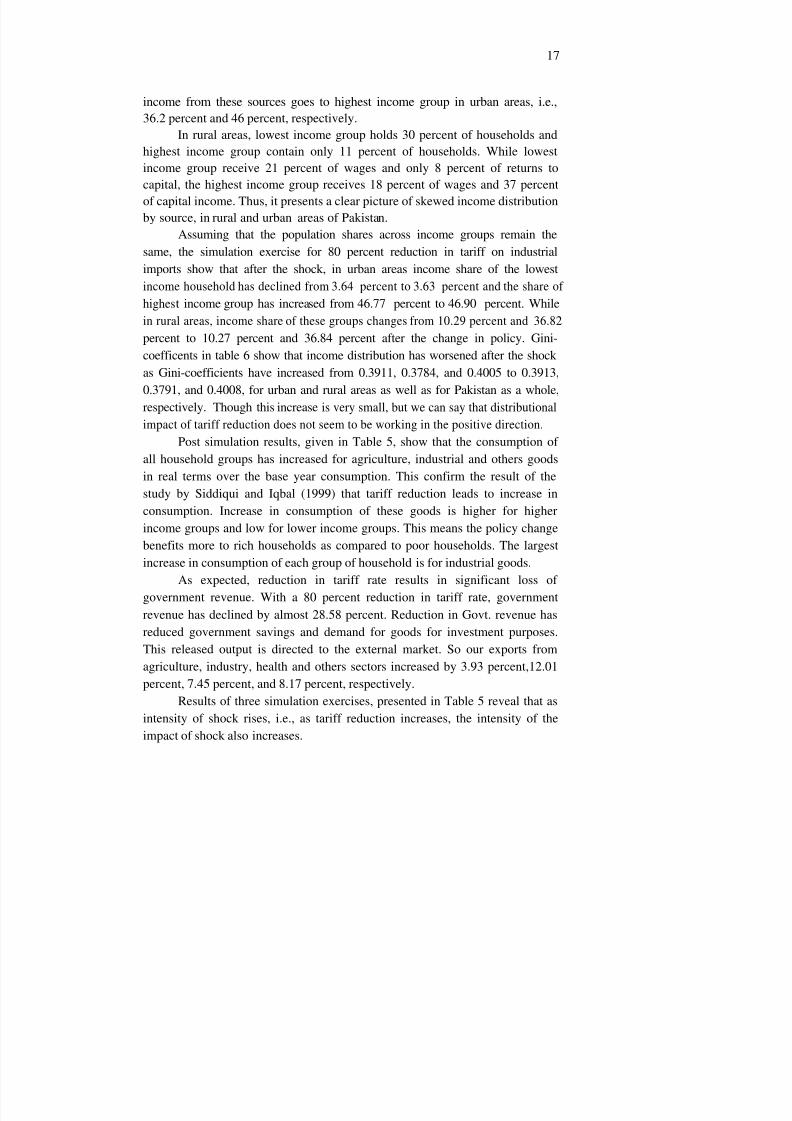
Assuming that the population shares across income groups remain the

same, the simulation exercise for 80 percent reduction in tariff on industrial

imports show that after the shock, in urban areas income share of the lowest

income household has declined from 3.64 percent to 3.63 percent and the share of

highest income group has increased from 46.77 percent to 46.90 percent. While

in rural areas, income share of these groups changes from 10.29 percent and 36.82

percent to 10.27 percent and 36.84 percent after the change in policy. Gini-

coefficents in table 6 show that income distribution has worsened after the shock

as Gini-coefficients have increased from 0.3911, 0.3784, and 0.4005 to 0.3913,

0.3791, and 0.4008, for urban and rural areas as well as for Pakistan as a whole,respectively. Though this increase is very small, but we can say that distributional

impact of tariff reduction does not seem to be working in the positive direction.

Post simulation results, given in Table 5, show that the consumption of

all household groups has increased for agriculture, industrial and others goods

in real terms over the base year consumption. This confirm the result of the

study by Siddiqui and Iqbal (1999) that tariff reduction leads to increase in

consumption. Increase in consumption of these goods is higher for higher

income groups and low for lower income groups. This means the policy change

benefits more to rich households as compared to poor households. The largest

increase in consumption of each group of household is for industrial goods.

As expected, reduction in tariff rate results in significant loss of

government revenue. With a 80 percent reduction in tariff rate, government

revenue has declined by almost 28.58 percent. Reduction in Govt. revenue has

reduced government savings and demand for goods for investment purposes.

This released output is directed to the external market. So our exports from

agriculture, industry, health and others sectors increased by 3.93 percent,12.01

percent, 7.45 percent, and 8.17 percent, respectively.

Results of three simulation exercises, presented in Table 5 reveal that as

intensity of shock rises, i.e., as tariff reduction increases, the intensity of the

impact of shock also increases.

8/8/2019 Report 181


18

VII. CONCLUSIONS

The study examines the impact of reduction in tariff on industrial imports

across households and on other broad macro aggregates. The simulation

exercises suggest that the impact of tariff rate reduction lowers the price of

imported goods, which affect the domestic relative output price and input price

structure. It affects supply and demand of all commodities. The tariff reduction increases the gap between the rich and poor as the

results show that share of capital and labour in GDP has increased and declined,

respectively. Consequently, Gini coefficients show that income distribution has

worsened. But impact on income distribution is very marginal.

The results also reveal that consumption of each household group has

increased. This implies that tariff reduction has welfare enhancing impact on

households. But increase in consumption of rich is greater than the increase in

consumption of poor. This implies that the policy change favors rich class and

benefits more to rich as compared to poor in terms of income as well as

consumption.

Decline in government revenue is responsible for low investment, which

ultimately affect economic activities adversely. This decline will have importantpolicy implication regarding identification of new avenues of resource

generation and reduction in fiscal deficit.

Appendices

APPENDIX I

I. CGE MODEL FOR PAKISTAN

Production Block

(1) is

= VAi / vi Production 5

(2) VAi =Bi [ i K I -

i+ (1- I )(L D

i)- i]-1/

i Production function(CES) 5

(3) IC i = io(i)*( VAi / vi) Intermediate Consumption of good I 5(4) IC ij = aij * ( i

s) Intermediate Consumption of good I in jth sector 25

(5) Li D = [{ i /(1- i)}{r/w}1/ +1 ]* Ki Labour Demand 5

Foreign Trade

(6) eS

= BT

e [ eT

EX eT + (1- e

T )De eT ] 1/

eT Export transformation (CET) 4

(7) Qc = Bsc [ c

s M - cs + (1- c

s )Dc-

cs ]1/

cs)

Import aggregation (Armington)(CES) 4

(8) Ex = (Pe / Pe D

)T

e [(1- eT

)/ eT ] T

e * De 4

(9) M c=(Pc D / Pc

M ) sc [( s

c /1-sc]

sc* Dc) Import Demand 4

(10) Q NT = X NT Demand for non traded good 1

(11) PcWM

*M c - (1 / e )T FR – PeW

*EX – e *T RH - e *T RG= e * CAB

Current Account Balance 1

8/8/2019 Report 181


19

Income and Saving

(12) Y H (h)=W l LiD+ RnK n+DIV(h)+ e *T RH (h)+ PINDEX*T GH (h)

Household Income 8

(13) YD H (h) = (1 - t y)*Y H (h) Household Disposable Income 8

(14) DIV (h)= dvr(h)*YF K Dividends 8

(15) S H (h)= mps(h)*YD H (h) Household saving 8 (16) Y FK = (1- ) (RiK i) Capital Income of Firms 1

(17) Y F = Y FK + PINDEX*T GF Firms total Income 1

(18) SF = Y F - T FR - DIV(h) - t k *Y FK Firms Saving 1

(19) TXS i = txi*Pi*X iS Indirect taxes 5

(20) TXM n = tmn* e * P nWM

M n Taxes on Imports 4

(21) TXE n = ten* e * P n E EX n Taxes on exports 4

(22) Y G = ty(h)*Y H (h)+ tk*Y FK + TXS i+ e *T RG+ TXM n + TXE n

Government Revenue 1

(23) SG = Y G –Pindex* T GF – Pindex * T GH (h)) – CT G

Government Saving 1

Demand

(24) C i (h) = iC (h)*CT H (h)/ Pi

C

Household Consumption for good I 40

(25) CT H (h)= YD H (h)- S H (h) Total Household Consumption 8

(26) INTDi = aij IC j Intermediate Demand 5

(27) CG i = i CT G /Pic Government Consumption 5

(28) C i = CT H (h)+ CGi Total Consumption of Good i 5

(29) I i = i I *IT/Pi

c Investment 5

Prices

(30) Ri = (PiVA

*VAi-W*Li D)/K i Returns to Capital 5

(31) Pn(1+ txi)* X ns = Dn

s*Pn D + (EX n)*Pn

E Value of output 4

(32) Pn

VA

*VAn= (Pn*X ns

) - (P j

C

IC ji) Value of Value Added 4(33) Pn

M = (1+tmn) * e * PnWM

Import Price 4

(34) Pn E = e * Pn

WE / (1+ten) Export Price 4

(35) PnC = (Dn /Qn)* Pn

D + (M n /Qn ) Pn M Composite price for composite good 4

(36) Pnt C = Pnt Price for non traded good 1

(37) Pindex= ( i X

* Pi) Price Index 1

Equilibrium

(38) IT = S H (h ) +SF + SG + e * CAB Saving Investment Equilibrium 1

(39) Qi = C i + INTDi + INV i Goods Market Equilibrium 5

(40) Ls = (Li D) Labour Market Equilibrium 1

Total Equations 215

8/8/2019 Report 181


20

II. VARIABLES

Endogenous Variables Definition Number of Variable

(1) Ci Total Consumption of Good 5

(2) CGi Public final Consumption of Good i 5

(3) CHi (h) Household h’s Consumption of Good i 40

(4) CTH (h) Total Consumption of household h 8

(5) Dn Domestic Demand for domestically produced good 4

(6) DIV (h) Dividends distributed to Households from firms 8

(7) EXn Exports of nth good (FOB) 4

(8) Mn Imports of nth good (CAF) 4

(9) ICi Total Intermediate Consumption of Good by ith sector 5

(10) ICJij Intermediate Consumption of Good J by ith sector 25

(11) INTDI Intermediate Demand of Good I 5

(12) INVi Consumption of Good by I for investment in sector i 5

(13) IT Total Investment 1

(14) LiD Labour Demand in sector i 5

(15) Pn Producer price 4

(16) PiC

Price of Composite good 5

(17) PnD Price of domestically produced and consumed good 4

(18) PnE Domestic price of Exports 4

(19) PnM Domestic Price of Imports 4

(20) PnVA Value Added Price 5

(21) PINDEX Producer price Index 1

(22) Qi Domestic Demand for Composite Good I 5

(23) Rn Rate of Return on capital in branch n 5

(24) S F Firms Saving 1

(25) S G Government Saving (Fiscal Deficit) 1

(26) SH (h) Saving of Household h 8

(27) TXEI Taxes on Imports of nth sector 4

(28) TXMi Taxes on Exports of nth sector 4

(29) TXSI Indirect taxes on ith sector production 5

(30) VAI Value Added of sector i 5

(31) Xis Production of ith sector 5

(32) YH (h) Total Income Household h 8

(33) YDH (h) Disposable income of h Households 8

(34) YF Firms total income 1

(35) YG Government Revenue 1

(36) YKF Firms Capital Income 1

(37) W Wage rate 1

Total Endogenous Variables 214

8/8/2019 Report 181


8/8/2019 Report 181


22

Appendix II

8/8/2019 Report 181


23

Appendix II

8/8/2019 Report 181


24

REFERENCES

Amjad, R., and A. R. Kemal (1997) Macroeconomic Policies and their Impact

on Poverty Alleviation in Pakistan. The Pakistan Development Review 36:1.

Bourguignon, et al. (1991) Modelling the Effects of Adjustment Programmes on

Income Distribution. World Development 19:11 1527–1544.

Decaluwe, B., M. C. Martin, and M. Souissi (1996) Ecole PARADI de modelisationde politiques economiques de development. Quebec, Universite Laval.

Pakistan, Government of (1997-98,1998-99) Economic Survey. Finance

Division, Islamabad.

Pakistan, Government of (1995-96) CBR, Year Book. Central Board of

Revenue, Islamabad.

Pakistan Government of (1994) The State of Pakistan’s Foreign Trade. Ministry

of Commerce.

Iqbal, Z. (1996) Three Gap Analysis of Structural Adjustment in Pakistan. Ph.D.

Dissertation. Tilburg University, the Netherlands (Unpublished).

Iqbal, Z., and R. Siddiqui (1999) The Impact of Structural Adjustment on

Income Distribution in Pakistan: A SAM-based Analysis. MIMAP Technical

Report No. 2. PIDE, Islamabad. Pakistan. Janvry. A. et al. (1991) Politically Feasible and Equitable Adjustment: Some

Alternatives for Ecuador. World Development 19:11 1577–1594.

James de Melo (1988) CGE Models for the analysis of Trade Policy in

Developing Countries. (Working Paper 144.)

Kemal, A. R. (1993) Recent Developments in the Manufacturing Sector of

Pakistan (an Industrial Sector Review Study). ADB.

Kemal, A. R. (1994) Structural Adjustment, Employment, Income Distribution

and Poverty. The Pakistan Development Review 33:4 901–911.

Khan, A. R. (1997) Globalisation, Liberalisation and Equitable Growth: Some

Lessons for Pakistan from Contemporary Asian Experience. The Pakistan

Development Review 36:4.

Labus, Miroljub (1988) A CGE Approach to Price Liberalisation Policy and

Public Sector Losses. Ljubljana.

Lambert, S. et al. (1991) Adjustment and Equity in Cote d’Ivoire: 1980-86.

World Development 19:11 1563–1576.

Mahmood, Zafar (1999) Pakistan Conditions Necessary for the Liberalisation of

Trade and Investment to Reduce Poverty. Unpublished Research Paper.

McGillivray, Mark, White Howard, and A. Afzal (1995) Evaluating the

Effectiveness of Structural Adjustment Policies on Macroeconomic

Performance: A Review of the Evidence with Special Reference to Pakistan.

The Pakistan Journal of Applied Economics 11:1& 2 57–76.

MCHD (1999) A Poverty Profile of Pakistan.

8/8/2019 Report 181


25

Meller, P. (1991) Adjustment and Social Costs in Chile During the 1980s.

World Development 19:11 1545–1561.

Morrisson, C. (1991) Adjustment, Income and Poverty in Morocco. World

Development 19:11 1633–1651.

Naqvi, Farzana (1997) Energy, Economy and Equity Interactions in a CGE

Model for Pakistan. Suffolk, UK.

Qureshi, S. K., and G. M. Arif (1999) The Poverty Profile of Pakistan.

Technical Report Prepared for MIMAP Project. PIDE, Islamabad.

Robinson, S. (1988) Multi sectoral Models. In H. B. Chenery and T. N.

Srinivassan (eds) Handbook of Development Economics Volume II.

Amsterdam: North-Holland. 885–947.

Siddiqui, Rizwana, and Zafar Iqbal (1999a) Social Accounting Matrix of

Pakistan for 1989-90. PIDE, Islamabad. (Research Report Series No 171.)

Siddiqui, Rizwana, and Zafar Iqbal (1999b) The Impact of Tariff Reduction on

Functional Income Distribution of Households: A CGE Model For Pakistan .

Presented in Regional Workshop on Modelling Structural Adjustment and

Income Distribution: CGE Framework, May 16-17.

Thorbecke, E. (1991) Adjustment, Growth and Income Distribution in

Indonesia. World Development 19:11 1595–1614.

Tilat, A. (1996) Structural Adjustment and Poverty: The Case of Pakistan. The

Pakistan Development Review 35:4 911–926.

White, H. (1997) The Economic and Social Impact of Adjustment in Africa:

Further Empirical Analysis. Unpublished.

World Bank (1995) Poverty Assessment . Washington, D.C.: The World Bank,

South Asia Region.

8/8/2019 Report 181


26

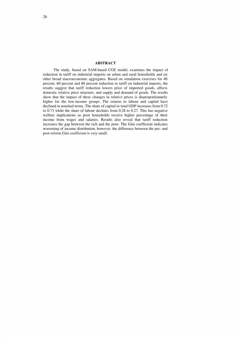
ABSTRACT

The study, based on SAM-based CGE model, examines the impact of

reduction in tariff on industrial imports on urban and rural households and on

other broad macroeconomic aggregates. Based on simulation exercises for 40

percent, 60 percent and 80 percent reduction in tariff on industrial imports, the

results suggest that tariff reduction lowers price of imported goods, affects

domestic relative price structure, and supply and demand of goods. The results

show that the impact of these changes in relative prices is disproportionately

higher for the low-income groups. The returns to labour and capital have

declined in nominal terms. The share of capital in total GDP increases from 0.72

to 0.73 while the share of labour declines from 0.28 to 0.27. This has negative

welfare implications as poor households receive higher percentage of their

income from wages and salaries. Results also reveal that tariff reduction

increases the gap between the rich and the poor. The Gini coefficient indicates

worsening of income distribution, however, the difference between the pre- and

post-reform Gini coefficient is very small.

8/8/2019 Report 181


This document was created with Win2PDF available at http://www.win2pdf.com.The unregistered version of Win2PDF is for evaluation or non-commercial use only.This page will not be added after purchasing Win2PDF.

http://www.win2pdf.com/





Documents

Report 181