Repeated Measures vs Randomized Blocks ANOVA

George H Olson, PhD

Appalachian State University

Original Version: Fall 2011

(Revised: Spring 2013, Spring 2014)

In the VassarStats textbook, Chapter 15 (One-way Analysis of Variance for Correlated

Samples), Part 1, you were introduced to two versions of ANOVA for correlated samples:

Repeated Measures ANOVA (RMAnova) and Randomized Blocks ANOVA (RBAnova).

One-way Designs

In a one-way RMAnova each subject is observed and measured under two or more

conditions. A general research design for a RMAnova can be depicted as shown below. In the

schematic, Xik represents the measurement for individual i under treatment k. In the design, each

of N subjects are exposed to all K treatments.

Table 1: Research Design for an N × K Repeated Measures ANOVA

Treatment 1 Treatment 2 Treatment 3 ∙ ∙ ∙ Treatment k ∙ ∙ ∙ Treatment K

Subject 1 X11 X12 X13 ∙ ∙ ∙ X1k ∙ ∙ ∙ X1K

Subject 2 X21 X22 X23 ∙ ∙ ∙ X2k ∙ ∙ ∙ X2K

∙

∙

∙

Subject i

∙

∙

∙

∙

∙

∙

Xi1

∙

∙

∙

∙

∙

∙

Xi2

∙

∙

∙

∙

∙

∙

Xi3

∙

∙

∙

∙ ∙ ∙ ∙ ∙ ∙ ∙

∙ ∙ ∙ ∙ ∙ ∙ ∙

∙ ∙ ∙ ∙ ∙ ∙ ∙

∙ ∙ ∙ Xik ∙ ∙ ∙ ∙ ∙ ∙ ∙ ∙ ∙ ∙

∙ ∙ ∙ ∙ ∙ ∙ ∙

∙ ∙ ∙ ∙ ∙ ∙ ∙

∙

∙

∙

XiK

∙

∙

∙

Subject N XN1 XN2 XN3 ∙ ∙ ∙ XNk ∙ ∙ ∙ XNK

The design for a one-way RBAnova is a little different, as shown in Table 2. In a true

randomized blocks design, the number of Blocks is equal to the number of measurements, or

times, that measurements are taken. Each Block contains K different subjects who are matched

on some characteristic. Hence, all the observations within a Block are assumed correlated. Also,

there is one subject in each Block × Treatment combination. Hence subjects are confounded with

Block × Time of Measurement combinations (the notation, Xiik, indicates a measurement for

individual i in Block k who is measured at Time k.) In a one-way RBAnova the notation could

be simplified by eliminating the first subscript for each observation. In other words, the notation,

Xiik, could have just as easily been written as Xik, providing it is understood that the second

subscript represents both the individual, i, and the Block, i. In this design, there are K×K

subjects1.

1 When considering more complex research designs, like those shown here, it is important to diagram the design,

including subscripts. Doing so helps the analyst keep track of what is being analyzed.

The advantage of the randomize blocks design is the same as that for a repeated measures

design and is adequately explained in Part 1 of VassarStats Chapter 15.

Table 2: Research Design for an K × K Randomized Blocks ANOVA

Measurement at Time k

1 2 3 ∙ ∙ ∙ k ∙ ∙ ∙ K

Block 1 X111

X212

X313

∙ ∙ ∙ Xk1k ∙ ∙ ∙

XK1K

Block 2 X121

X222

X223

∙ ∙ ∙ X22k ∙ ∙ ∙

X22K

Block 3 X331

X332

X333

∙ ∙ ∙ X33k ∙ ∙ ∙

X33K

∙

∙

∙

Block j

∙

∙

∙

∙

∙

∙

Xjj1

∙

∙

∙

∙

∙

∙

Xjj2

∙

∙

∙

∙

∙

∙

Xjj3

∙

∙

∙

∙ ∙ ∙ ∙ ∙ ∙ ∙

∙ ∙ ∙ ∙ ∙ ∙ ∙

∙ ∙ ∙ ∙ ∙ ∙ ∙

∙ ∙ ∙ Xjjk ∙ ∙ ∙

∙ ∙ ∙ ∙ ∙ ∙ ∙

∙ ∙ ∙ ∙ ∙ ∙ ∙

∙ ∙ ∙ ∙ ∙ ∙ ∙

∙ ∙ ∙

∙ ∙ ∙

∙ ∙ ∙

XjjK

∙ ∙ ∙

∙ ∙ ∙

∙ ∙ ∙

∙ ∙ ∙

Block K XKK1 XKK2 XKK3 ∙ ∙ ∙ XKKk ∙ ∙ ∙ XKKK

J-Between, K-Within Designs

Often, in practice, in an RMAnova design, we might have two or more (or J) groups of

individuals –representing two or more levels of an independent variable—on whom a common

set of K repeated measurements are taken. Similarly, in an RBAnova design, we might have two

or J blocks if individuals–representing two or K levels of an independent variable—on whom a

common set of measurements are taken. The difference is that in the RMAnova the same

individuals are measured repeatedly, whereas in the RBAnova design different individuals

matched on some characteristic are measured on the K different occasions.

A research design for a J-Between, K-Within RMAnova is depicted in Table 3, where it

is assumed that Factor A has K levels. Since different individuals are measured in each level of

Factor A, Factor A is referred to as a between groups factor. The repeated measures, on the other

hand, are measured within individuals; hence the repeated measures factor is referred to as a

within groups factor.

In Table 3 the notation, Xijk, denotes kth

measure taken on the ith

individual in group at

level Aj. We often refer to this design as a one-between, one-within design. It should be obvious

that more complex designs are possible. For instance, a two-between, one-within design would

have two between-groups factors, A and B, for instance, and one within-groups factor

(measures). Similarly, a two-between, two-within design would have two between-groups factors

and two sets of repeated measures, taken under two conditions (before lunch and after lunch, for

instance.)

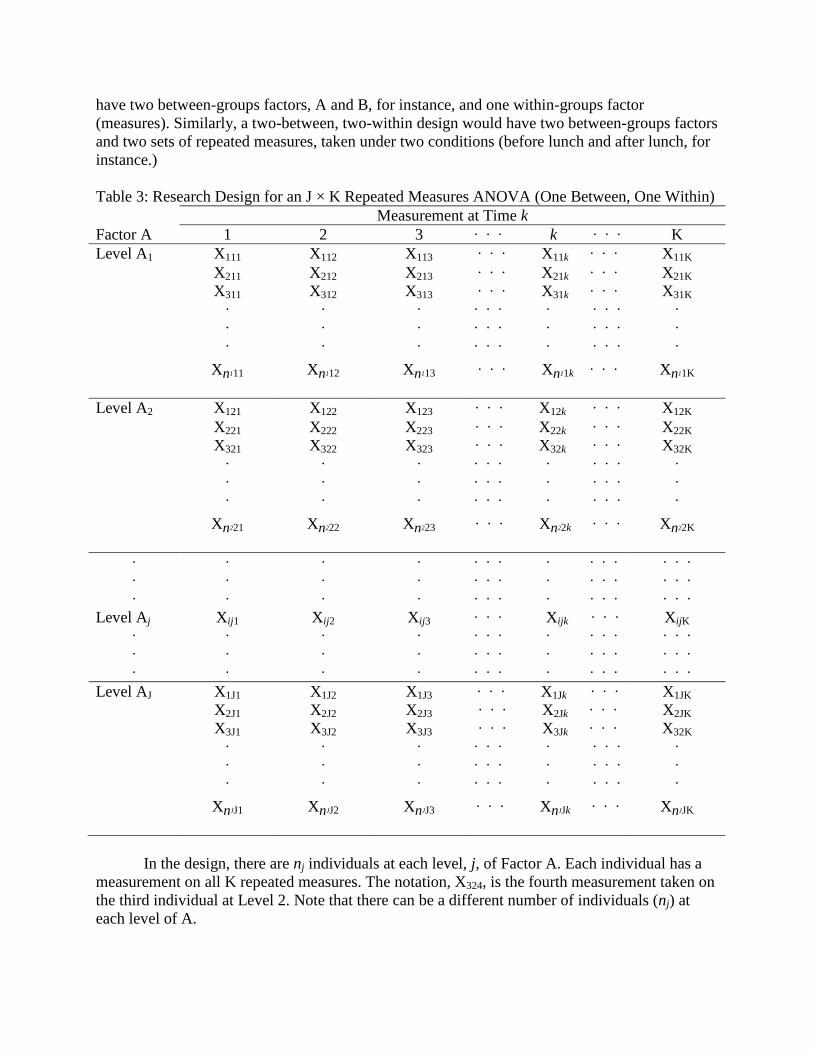
Table 3: Research Design for an J × K Repeated Measures ANOVA (One Between, One Within)

Measurement at Time k

Factor A 1 2 3 ∙ ∙ ∙ k ∙ ∙ ∙ K

Level A1 X111 X112 X113 ∙ ∙ ∙ X11k ∙ ∙ ∙ X11K

X211 X212 X213 ∙ ∙ ∙ X21k ∙ ∙ ∙ X21K

X311 X312 X313 ∙ ∙ ∙ X31k ∙ ∙ ∙ X31K

∙

∙

∙

∙

∙

∙

∙

∙

∙

∙ ∙ ∙ ∙ ∙ ∙ ∙

∙ ∙ ∙ ∙ ∙ ∙ ∙

∙ ∙ ∙ ∙ ∙ ∙ ∙

∙

∙

∙

Xn111 Xn112 Xn113 ∙ ∙ ∙ Xn11k ∙ ∙ ∙ Xn11K

Level A2 X121 X122 X123 ∙ ∙ ∙ X12k ∙ ∙ ∙ X12K

X221 X222 X223 ∙ ∙ ∙ X22k ∙ ∙ ∙ X22K

X321 X322 X323 ∙ ∙ ∙ X32k ∙ ∙ ∙ X32K

∙

∙

∙

∙

∙

∙

∙

∙

∙

∙ ∙ ∙ ∙ ∙ ∙ ∙

∙ ∙ ∙ ∙ ∙ ∙ ∙

∙ ∙ ∙ ∙ ∙ ∙ ∙

∙

∙

∙

Xn221 Xn222 Xn223 ∙ ∙ ∙ Xn22k ∙ ∙ ∙ Xn22K

∙

∙

∙

Level Aj

∙

∙

∙

∙

∙

∙

Xij1

∙

∙

∙

∙

∙

∙

Xij2

∙

∙

∙

∙

∙

∙

Xij3

∙

∙

∙

∙ ∙ ∙ ∙ ∙ ∙ ∙

∙ ∙ ∙ ∙ ∙ ∙ ∙

∙ ∙ ∙ ∙ ∙ ∙ ∙

∙ ∙ ∙ Xijk ∙ ∙ ∙

∙ ∙ ∙ ∙ ∙ ∙ ∙

∙ ∙ ∙ ∙ ∙ ∙ ∙

∙ ∙ ∙ ∙ ∙ ∙ ∙

∙ ∙ ∙

∙ ∙ ∙

∙ ∙ ∙

XijK

∙ ∙ ∙

∙ ∙ ∙

∙ ∙ ∙

Level AJ X1J1 X1J2 X1J3 ∙ ∙ ∙ X1Jk ∙ ∙ ∙ X1JK

X2J1 X2J2 X2J3 ∙ ∙ ∙ X2Jk ∙ ∙ ∙ X2JK

X3J1 X3J2 X3J3 ∙ ∙ ∙ X3Jk ∙ ∙ ∙ X32K

∙

∙

∙

∙

∙

∙

∙

∙

∙

∙ ∙ ∙ ∙ ∙ ∙ ∙

∙ ∙ ∙ ∙ ∙ ∙ ∙

∙ ∙ ∙ ∙ ∙ ∙ ∙

∙

∙

∙

XnJJ1 XnJJ2 XnJJ3 ∙ ∙ ∙ XnJJk ∙ ∙ ∙ XnJJK

In the design, there are nj individuals at each level, j, of Factor A. Each individual has a

measurement on all K repeated measures. The notation, X324, is the fourth measurement taken on

the third individual at Level 2. Note that there can be a different number of individuals (nj) at

each level of A.

A research design of an J x K RBAnova design is similar to the RMAnova design except

that instead of levels of a between-group factor we have different blocks of similar (presumably

matched) individuals. The blocks could represent different levels of some independent variable

as in the RMAnova design. The main difference between the two designs is that in the RBAnova

design all the Xijk represent different measures on different individuals. Hence, Xijk, represents

the kth

measurement on the i’th subject in Block j.

Table 4: Research Design for an J × K Randomized Blocks ANOVA

Measurement at Time k

Factor A 1 2 3 ∙ ∙ ∙ k ∙ ∙ ∙ K

Block 1 X111 X112 X113 ∙ ∙ ∙ X11k ∙ ∙ ∙ X11K

X211 X212 X213 ∙ ∙ ∙ X21k ∙ ∙ ∙ X21K

X311 X312 X313 ∙ ∙ ∙ X31k ∙ ∙ ∙ X31K

∙

∙

∙

∙

∙

∙

∙

∙

∙

∙ ∙ ∙ ∙ ∙ ∙ ∙

∙ ∙ ∙ ∙ ∙ ∙ ∙

∙ ∙ ∙ ∙ ∙ ∙ ∙

∙

∙

∙

Xn111 Xn112 Xn113 ∙ ∙ ∙ Xn11k ∙ ∙ ∙ Xn11K

Block 2 X121 X122 X123 ∙ ∙ ∙ X12k ∙ ∙ ∙ X12K

X221 X222 X223 ∙ ∙ ∙ X22k ∙ ∙ ∙ X22K

X321 X322 X323 ∙ ∙ ∙ X32k ∙ ∙ ∙ X32K

∙

∙

∙

∙

∙

∙

∙

∙

∙

∙ ∙ ∙ ∙ ∙ ∙ ∙

∙ ∙ ∙ ∙ ∙ ∙ ∙

∙ ∙ ∙ ∙ ∙ ∙ ∙

∙

∙

∙

Xn221 Xn222 Xn223 ∙ ∙ ∙ Xn22k ∙ ∙ ∙ Xn22K

∙

∙

∙

Block j

∙

∙

∙

∙

∙

∙

Xij1

∙

∙

∙

∙

∙

∙

Xij2

∙

∙

∙

∙

∙

∙

Xij3

∙

∙

∙

∙ ∙ ∙ ∙ ∙ ∙ ∙

∙ ∙ ∙ ∙ ∙ ∙ ∙

∙ ∙ ∙ ∙ ∙ ∙ ∙

∙ ∙ ∙ Xijk ∙ ∙ ∙

∙ ∙ ∙ ∙ ∙ ∙ ∙

∙ ∙ ∙ ∙ ∙ ∙ ∙

∙ ∙ ∙ ∙ ∙ ∙ ∙

∙ ∙ ∙

∙ ∙ ∙

∙ ∙ ∙

XijK

∙ ∙ ∙

∙ ∙ ∙

∙ ∙ ∙

Block J X1J1 X1J2 X1J3 ∙ ∙ ∙ X1Jk ∙ ∙ ∙ X1JK

X2J1 X2J2 X2J3 ∙ ∙ ∙ X2Jk ∙ ∙ ∙ X2JK

X3J1 X3J2 X3J3 ∙ ∙ ∙ X3Jk ∙ ∙ ∙ X32K

∙

∙

∙

∙

∙

∙

∙

∙

∙

∙ ∙ ∙ ∙ ∙ ∙ ∙

∙ ∙ ∙ ∙ ∙ ∙ ∙

∙ ∙ ∙ ∙ ∙ ∙ ∙

∙

∙

∙

XnJJ1 XnJJ2 XnJJ3 ∙ ∙ ∙ XnJJk ∙ ∙ ∙ XnJJK

As in the case of RMAnova the number of subjects within a block can vary across blocks.

Hence, while block 2 may have n2 subjects, block K might have nK subjects.

An Example: Randomized Blocks Repeated Measures Design

In this factitious example we have a researcher who wants to investigate the effects of three types of instruction: Face to Face (F2F), Virtual Face to Face (V-F2F) via an immersive virtual environment (e.g., Appstate’s Open Qwaq), and asynchronous online (AsyOL). She has 23 students in the particular class in which she wants to conduct her study. One approach she could use is to randomly assign the 23 students to the three conditions as follows:

Table 5: One Possible Scenario for Using 23 Subjects

Instructional Condition F2F V-F2F AsyOL Number of students 8 8 7

However, she realizes that there could be considerable variance due to individual

differences among students assigned to each condition (random assignment does not mitigate this potential problem). This could result in inflated within-group variance, leading to weakened power. Instead, she opts to employ a repeated-measures design where all 23 students are exposed to all three instructional conditions.

She realizes, also, that order of exposure to the three conditions may have a systematic

effect on the students’ achievement outcomes. For instance, exposure to F3F first might influence how students later react to V-F2F. Additionally, it is not unreasonable to assume that there may be a sequential, cumulative effect to the instructional conditions. For instance, regardless of which condition students are exposed to first, that exposure might affect their reaction to the second condition exposure, and so on. With this realization, she decides to employ a variation of a randomized blocks with repeated measures design. The design looks like that depicted in the table on the next page.

There are three blocks, each having a different sequence of instructional conditions:

BLOCK 1: F2F, first, followed by V-F2F, followed by AsyOL, BLOCK 2: V-F2F, first, followed by AsyOL followed by F2F, BLOCK 3: AsyOL first, followed by F2F, followed by V-F2F.

Other sequences are, of course, possible. However, one of the things she is particularly

interested in is the carry-over effect of F2F on V-F2F and AsyOL. Based on her previous experience with online instruction, she hypothesizes that F2F instruction has a positive influence on students’ reaction to exposure to the two types of online instruction. She randomly assigns students to the three blocks (eight students to each of the first two blocks, and seven to the BLOCK 3. Within each block, students are exposed to each of the three instructional conditions, in order, for five weeks. At the end of each five weeks, she administers a 25-item achievement test over the content covered during the previous five weeks. Hence, she collects achievement data three times over the 15-week semester. It should

be noted that as the semester progresses, all students cover the same content regardless of their sequence of instructional exposure.

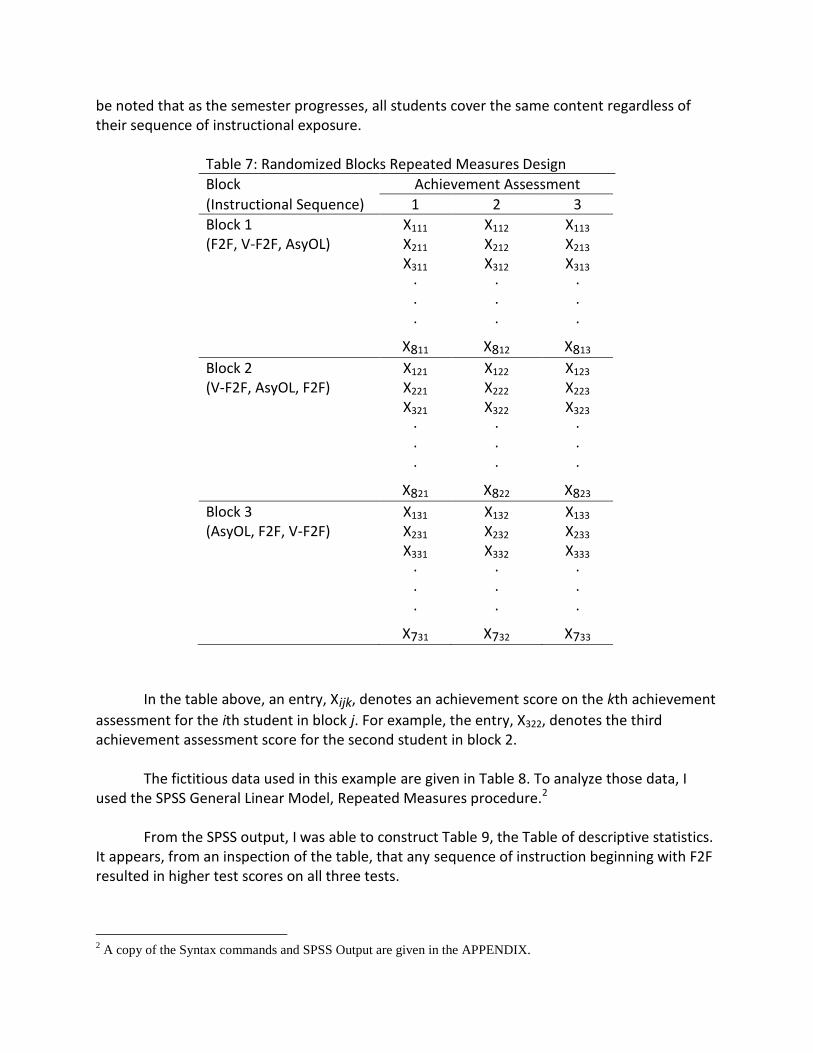
Table 7: Randomized Blocks Repeated Measures Design

Block Achievement Assessment

(Instructional Sequence) 1 2 3

Block 1 X111 X112 X113 (F2F, V-F2F, AsyOL) X211 X212 X213 X311 X312 X313 ∙

∙ ∙

∙ ∙ ∙

∙ ∙ ∙

X811 X812 X813

Block 2 X121 X122 X123 (V-F2F, AsyOL, F2F) X221 X222 X223 X321 X322 X323 ∙

∙ ∙

∙ ∙ ∙

∙ ∙ ∙

X821 X822 X823

Block 3 X131 X132 X133 (AsyOL, F2F, V-F2F) X231 X232 X233 X331 X332 X333 ∙

∙ ∙

∙ ∙ ∙

∙ ∙ ∙

X731 X732 X733

In the table above, an entry, Xijk, denotes an achievement score on the kth achievement

assessment for the ith student in block j. For example, the entry, X322, denotes the third achievement assessment score for the second student in block 2. The fictitious data used in this example are given in Table 8. To analyze those data, I used the SPSS General Linear Model, Repeated Measures procedure.2 From the SPSS output, I was able to construct Table 9, the Table of descriptive statistics. It appears, from an inspection of the table, that any sequence of instruction beginning with F2F resulted in higher test scores on all three tests.

2 A copy of the Syntax commands and SPSS Output are given in the APPENDIX.

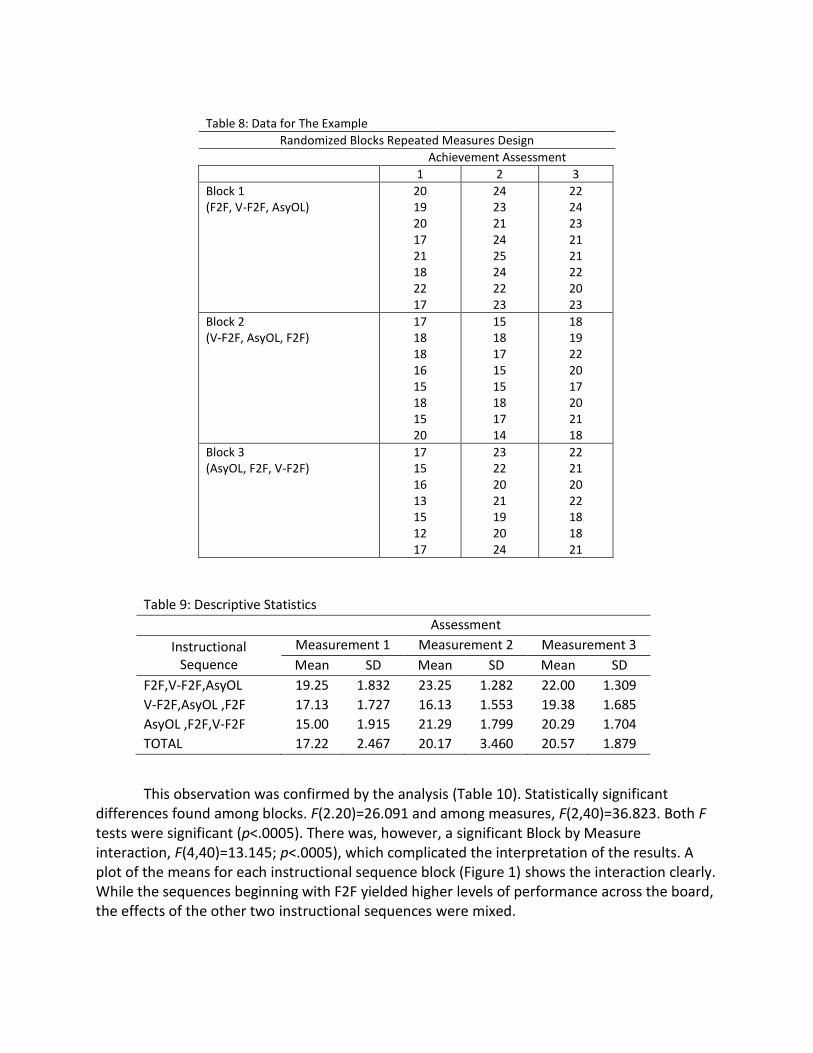
Table 8: Data for The Example

Randomized Blocks Repeated Measures Design

Achievement Assessment

1 2 3

Block 1 (F2F, V-F2F, AsyOL)

20 19 20 17 21 18 22 17

24 23 21 24 25 24 22 23

22 24 23 21 21 22 20 23

Block 2 (V-F2F, AsyOL, F2F)

17 18 18 16 15 18 15 20

15 18 17 15 15 18 17 14

18 19 22 20 17 20 21 18

Block 3 (AsyOL, F2F, V-F2F)

17 15 16 13 15 12 17

23 22 20 21 19 20 24

22 21 20 22 18 18 21

Table 9: Descriptive Statistics

Assessment

Instructional Sequence

Measurement 1 Measurement 2 Measurement 3

Mean SD Mean SD Mean SD

F2F,V-F2F,AsyOL 19.25 1.832 23.25 1.282 22.00 1.309

V-F2F,AsyOL ,F2F 17.13 1.727 16.13 1.553 19.38 1.685

AsyOL ,F2F,V-F2F 15.00 1.915 21.29 1.799 20.29 1.704

TOTAL 17.22 2.467 20.17 3.460 20.57 1.879

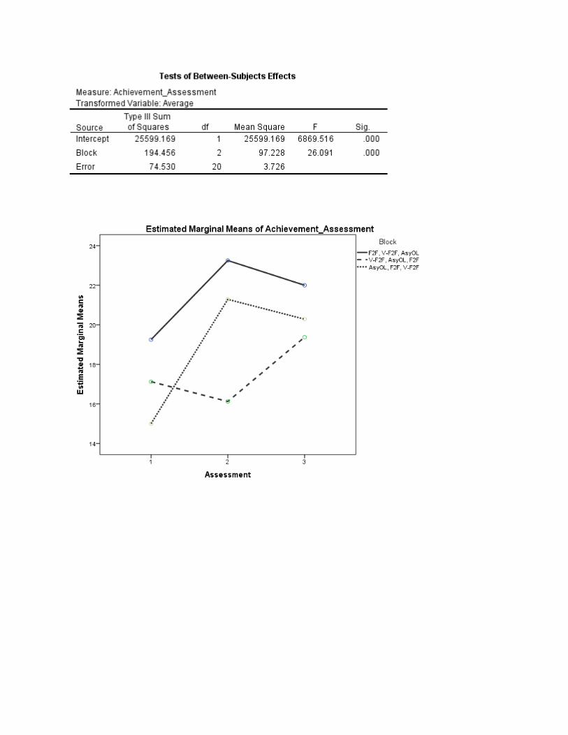
This observation was confirmed by the analysis (Table 10). Statistically significant differences found among blocks. F(2.20)=26.091 and among measures, F(2,40)=36.823. Both F tests were significant (p<.0005). There was, however, a significant Block by Measure interaction, F(4,40)=13.145; p<.0005), which complicated the interpretation of the results. A plot of the means for each instructional sequence block (Figure 1) shows the interaction clearly. While the sequences beginning with F2F yielded higher levels of performance across the board, the effects of the other two instructional sequences were mixed.

Table 10: Analysis of Variance Summary Table

Source SS df MS F Sig

Between Subjects

Blocks (B) 194.456 2 97.228 26.091 <.0005

Error 74.530 20 3.726

Within Subjects

Measures. (M) 163.775 2 81.887 36.823 <.0005

B x M 116.932 4 29.233 13.145 <.0005

Error (w/ groups) 188.952 40 .4082.224

On the first test, the group receiving virtual F2F instruction first outperformed the group receiving asynchronous online instruction. By the second assessment, the effects of V-F2F and AsyOL were reversed, with the group receiving asynchronous instruction out performing those receiving virtual F2F instruction. While this difference persisted at the third assessment, the difference between the two groups was not as great.

Figure 1: Assessment scores by Instructional Sequence Block

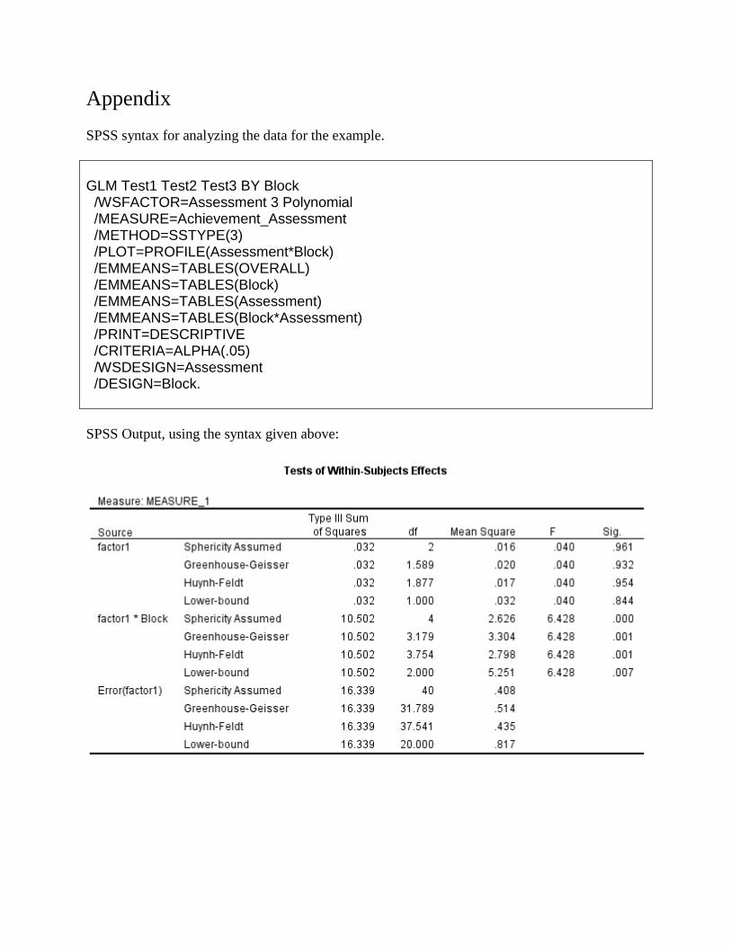
Appendix

SPSS syntax for analyzing the data for the example.

GLM Test1 Test2 Test3 BY Block /WSFACTOR=Assessment 3 Polynomial /MEASURE=Achievement_Assessment /METHOD=SSTYPE(3) /PLOT=PROFILE(Assessment*Block) /EMMEANS=TABLES(OVERALL) /EMMEANS=TABLES(Block) /EMMEANS=TABLES(Assessment) /EMMEANS=TABLES(Block*Assessment) /PRINT=DESCRIPTIVE /CRITERIA=ALPHA(.05) /WSDESIGN=Assessment /DESIGN=Block.

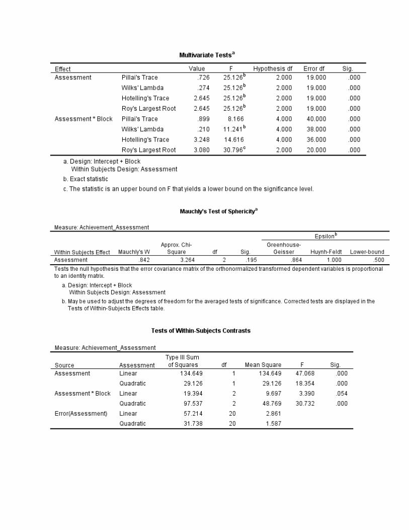
SPSS Output, using the syntax given above: