Embed Size (px)
Citation preview

05
10C
hi-s
quar
e0
510
Chi
-squ
are
Repeated Measures, Part 2
May, 2009
Charles E. McCulloch, Division of Biostatistics,Dept of Epidemiology and Biostatistics,UCSF

2
05
10C
hi-s
quar
e0
510
Chi
-squ
are
Outline
1. Fixed and random factors2. XT - preliminaries3. XTMIXED for continuous outcomes4. Other uses of random effects models5. XTGEE for a variety of outcome types6. Model checking7. Summary

3
05
10C
hi-s
quar
e0
510
Chi
-squ
are
Fixed versus Random Factors
Models for correlated data are often specified by declaring one or more of the categorical predictors in the model to be random factors. (Otherwise they are called fixed factors.) Models with both fixed and random factors are called mixed models.
The name of the Stata command for approximately normally distributed outcomes is XTMIXED. The X is for cross-sectional, the T for time series and MIXED for mixed model.
Definition: If a distribution is assumed for the effects associated with the levels of a factor it is random. If the values are fixed, unknown constants it is a fixed factor.

4
05
10C
hi-s
quar
e0
510
Chi
-squ
are
Fixed versus Random Factors
Are we willing to assume that the effects associated with the levels of a factor can be regarded as a random sample from some reasonable population of effects. (If yes then random, if no then fixed).
This is what we ordinarily do for any sample – we ask if we can regard it as a random sample from a larger population. For hierarchical data structures we ask the question over again for each level.

5
05
10C
hi-s
quar
e0
510
Chi
-squ
are
Notes on fixed vs random Factors1. Continuous variables are virtually never random effects. We
typically treat a variable as continuous because knowing the outcome for one value of the variable tells us something about the nearby values (hence the effects are not random). Do not confuse this with the fact that, if we have a random sample of subjects, their ages are a random sample of ages.
2. Scope of inference: Inferences can be made on a statistical basis to the population from which the levels of the random factor have been selected.
3. Incorporation of correlation in the model: Observations that share the same level of the random effect are being modeled as correlated.
4. Accuracy of estimates: Using random factors involves making extra assumptions but gives more accurate estimates.
5. Estimation method: Different estimation methods must be used.

6
05
10C
hi-s
quar
e0
510
Chi
-squ
are
Fixed versus Random Practice Fecal fat example. Factors? Fixed?
Random?
Back pain example. Factors? Fixed? Random?
Study of Osteoporotic Fractures. Factors? Fixed? Random?

7
05
10C
hi-s
quar
e0
510
Chi
-squ
are
Preliminaries: xtset, xtdescribe
Before using an XT command you should tell Stata how the data are clustered using the xtset command:
xtset clustering variable “time” variable And it is often worthwhile to understand the
patterns of present/absent data using xtdescribe

8
05
10C
hi-s
quar
e0
510
Chi
-squ
areExample: HERS
Heart and Estrogen/Progestin Study (HERS - Hulley, et al, 1998, JAMA), was a randomized trial with long-term, yearly followup. pptid is the participant ID and nvisit is the visit number, with 0 being baseline:
. xtset pptid nvisit panel variable: pptid (unbalanced) time variable: nvisit, 0 to 5, but with gaps delta: 1 unit

9
05
10C
hi-s
quar
e0
510
Chi
-squ
areExample: HERS
. xtdescribe pptid: 1, 2, ..., 2763 n = 2763 nvisit: 0, 1, ..., 5 T = 6 Delta(nvisit) = 1 unit Span(nvisit) = 6 periods (pptid*nvisit uniquely identifies each observation)
Distribution of T_i: min 5% 25% 50% 75% 95% max 1 2 4 5 5 6 6
Freq. Percent Cum. | Pattern ---------------------------+--------- 1469 53.17 53.17 | 11111. 531 19.22 72.39 | 1111.. 327 11.83 84.22 | 111111 119 4.31 88.53 | 111... 106 3.84 92.36 | 1..... 87 3.15 95.51 | 11.... 40 1.45 96.96 | 111.1. 22 0.80 97.76 | 1111.1 11 0.40 98.15 | 11.11. 51 1.85 100.00 | (other patterns) ---------------------------+--------- 2763 100.00 | XXXXXX

10
05
10C
hi-s
quar
e0
510
Chi
-squ
are
xtmixed is for approximately normally distributed outcomes. Here is the command syntax:
xtmixed depvar fix_effects || rand_ effects: , cov(corr structure)
Example: Georgia babies
xtmixed bweight birthord initage||momid:
XTMIXED for continuous outcomes
Punctuation important!

11
05
10C
hi-s
quar
e0
510
Chi
-squ
are
XTMIXED for continuous outcomes
There can be multiple random effects specified by adding additional ||’s and random effects at the end.
In this way you can handle multiple hierarchies or levels of clustering. Order is from highest to lowest level of clustering.
Example: backpain data
xi:xtmixed logcost i.pracstyl i.educ || doctor: || patient:

12
05
10C
hi-s
quar
e0
510
Chi
-squ
are
XTMIXED for continuous outcomes
Specifying a random factor with a colon tells XTMIXED to allow different intercepts for each level of the factor, e.g., different intercepts for each patient.
This is often sufficient, but there are cases in which more features of the model need to be included, for example, patient, animal or physician specific terms.
If so, these are added after the colon.

13
05
10C
hi-s
quar
e0
510
Chi
-squ
are
Mouse tumor/weight data
45
67
84
56
78
45
67
84
56
78
0 20 40 60
0 20 40 60 0 20 40 60 0 20 40 60
26 27 28 29
30 31 32 33
34 35 36 37
38 39 40
Log
Weig
ht
DayGraphs by mouse
For a single treatment groupMouse-specific trajectories of log(weight)
How do these compare?
14
05
10C
hi-s
quar
e0
510
Chi
-squ
are
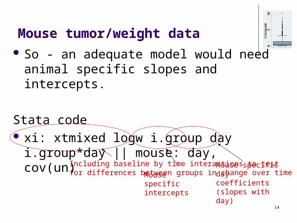
Including baseline by time interactions to test for differences between groups in change over time
Mouse tumor/weight data So - an adequate model would need animal
specific slopes and intercepts.
Stata code xi: xtmixed logw i.group day i.group*day || mouse: day, cov(un)
Mouse specific intercepts
Mouse specific day coefficients (slopes with day)

15
05
10C
hi-s
quar
e0
510
Chi
-squ
are
Mouse tumor/weight data
More details in lab, but the “|| mouse:” portion specifies that mouse is a random effect (i.e., allows a mouse specific intercept) and the “day” term specifies that the slopes over days that are associated with a mouse are also random effects.
The “cov(un)” specifies that the variance and covariances of the random intercepts and slopes are unstructured. That is, the variances of the random intercepts and slopes are not assumed the same and they may be correlated.

16
05
10C
hi-s
quar
e0
510
Chi
-squ
are
Recall: Fecal fat example Fecal Fat (g/day) Pill type PatID/ Sex
None Tablet Capsule Coated Capsule
Avg
1 – M 44.5 7.3 3.4 12.4 16.900 2 – M 33.0 21.0 23.1 25.4 25.625 3 – M 19.1 5.0 11.8 22.0 14.475 4 – F 9.4 4.6 4.6 5.8 6.100 5 – F 71.3 23.3 25.6 68.2 47.100 6 – F 51.2 38.0 36.0 52.6 44.450 Avg 38.08 16.53 17.42 31.07 25.775

17
05
10C
hi-s
quar
e0
510
Chi
-squ
are
Mixed-effects REML regression Number of obs = 24Group variable: patid Number of groups = 6 Obs per group: min = 4 avg = 4.0 max = 4 Wald chi2(3) = 18.77Log restricted-likelihood = -84.555945 Prob > chi2 = 0.0003------------------------------------------------------------------------------ fecfat | Coef. Std. Err. z P>|z| [95% Conf. Interval]-------------+----------------------------------------------------------------_Ipilltype_2 | -21.55 5.972127 -3.61 0.000 -33.25515 -9.844848_Ipilltype_3 | -20.66667 5.972127 -3.46 0.001 -32.37182 -8.961514_Ipilltype_4 | -7.016668 5.972127 -1.17 0.240 -18.72182 4.688485 _cons | 38.08333 7.742396 4.92 0.000 22.90852 53.25815------------------------------------------------------------------------------------------------------------------------------------------------------------ Random-effects Parameters | Estimate Std. Err. [95% Conf. Interval]-----------------------------+------------------------------------------------patid: Identity | sd(_cons) | 15.89557 5.567268 8.00113 31.5792-----------------------------+------------------------------------------------ sd(Residual) | 10.34403 1.888552 7.232396 14.79439------------------------------------------------------------------------------LR test vs. linear regression: chibar2(01) = 12.52 Prob >= chibar2 = 0.0002
xtmixed for the fecal fat exampleSummary information about hierarchy
Summary of variation in random intercepts ( sd(_cons) )and residuals ( sd(Residual) )
Test of H0: no clustering
The usual coef and SE

18
05
10C
hi-s
quar
e0
510
Chi
-squ
are
Mixed model analyses
You get estimates of the regression coefficients (with the same interpretation as in regular regression), but accounting for the correlated data.
Also get an understanding of how the variability in the data is attributable to various levels in the hierarchy.

19
05
10C
hi-s
quar
e0
510
Chi
-squ
are
Mixed model analyses
Total variance = sum of all estimated variances.
Total variance = (patient SD)2+(residual SD)2
= (15.89557)2 + (10.34403)2
= 252.6691+ 106.9990 = 359.6681• Intraclass correlation (ICC)
ICC = (patient SD)2/(total variance)
= 252.6691/359.6681 = 0.703

20
05
10C
hi-s
quar
e0
510
Chi
-squ
are
Non-normally distributed outcomes
Stata can also handle non-normally distributed outcomes and other types of regression models, for example logistic regression. The most common method of analysis for non-normally distributed data is a very flexible method called “generalized estimating equations” or GEEs. The corresponding Stata command is called XTGEE. It can also handle (and we will start with) normally distributed outcomes.
GEEs work by estimating the correlation structure in the data from replications across subjects (as opposed to modeling it with random effects).

21
05
10C
hi-s
quar
e0
510
Chi
-squ
are
Terminology
GEE type models are sometimes called “population averaged” or “marginal” models because they hypothesize a relationship (e.g., logistic regression) that holds averaged over all subjects in a population. Random effects models (like those fit by XTMIXED) are sometimes called “subject specific” or “conditional” because they are built using random effects that are specific to a subject (e.g., a doctor or mouse effect).

22
05
10C
hi-s
quar
e0
510
Chi
-squ
are
Using xtgee: 5 things to specify
1. What is the distributional family (for fixed values of the covariates) that is appropriate to use for the outcome data? Normal, binary, binomial (other?).
2. Which predictors are we going to include in the model? (Nothing new here).
3. In what way are we going to link the predictors to the data? (Through the mean? Through the logit of the risk?)
4. What correlation structure will be used or assumed temporarily in order to form the estimates?
5. Which variable indicates how the data are clustered?
23
05
10C
hi-s
quar
e0
510
Chi
-squ
are
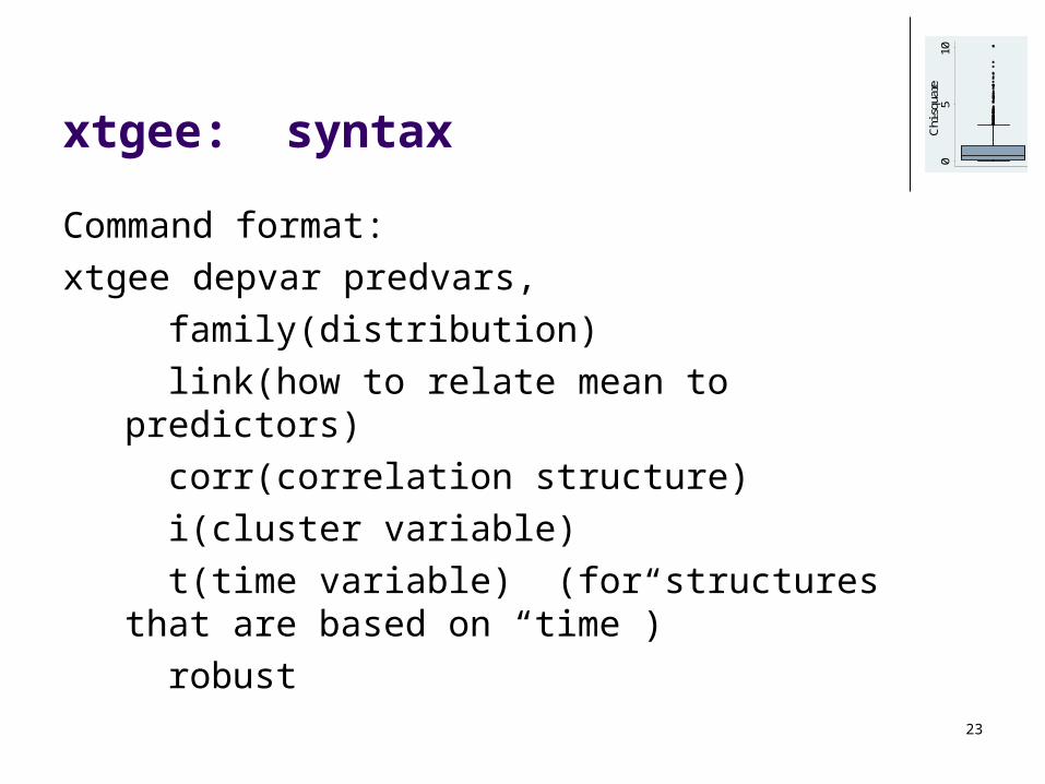
xtgee: syntax
Command format:
xtgee depvar predvars,
family(distribution)
link(how to relate mean to predictors)
corr(correlation structure)
i(cluster variable)
t(time variable) (for structures that are based on “time”)
robust

24
05
10C
hi-s
quar
e0
510
Chi
-squ
are
xtgee: syntax
Example: Fecal Fat
xi: xtgee fecfat i.pilltype i.sex, i(patid) t(pilltype) family(gaussian) corr(exch)
which can be shortened using defaults to
xi: xtgee fecfat i.pilltype i.sex, i(patid)
25
05
10C
hi-s
quar
e0
510
Chi
-squ
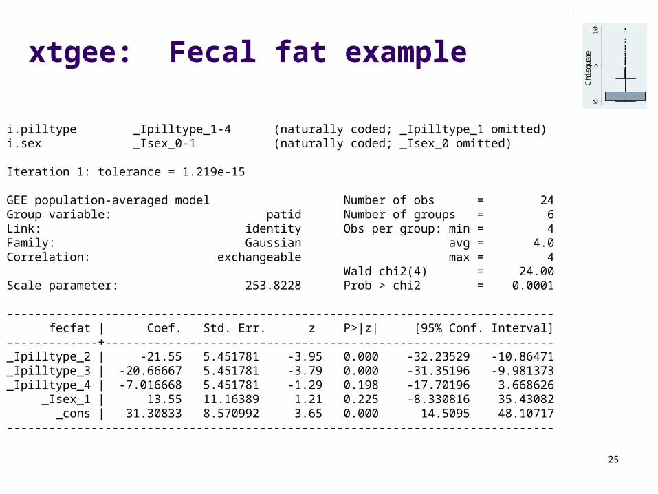
arextgee: Fecal fat example
i.pilltype _Ipilltype_1-4 (naturally coded; _Ipilltype_1 omitted)i.sex _Isex_0-1 (naturally coded; _Isex_0 omitted)
Iteration 1: tolerance = 1.219e-15
GEE population-averaged model Number of obs = 24Group variable: patid Number of groups = 6Link: identity Obs per group: min = 4Family: Gaussian avg = 4.0Correlation: exchangeable max = 4 Wald chi2(4) = 24.00Scale parameter: 253.8228 Prob > chi2 = 0.0001
------------------------------------------------------------------------------ fecfat | Coef. Std. Err. z P>|z| [95% Conf. Interval]-------------+----------------------------------------------------------------_Ipilltype_2 | -21.55 5.451781 -3.95 0.000 -32.23529 -10.86471_Ipilltype_3 | -20.66667 5.451781 -3.79 0.000 -31.35196 -9.981373_Ipilltype_4 | -7.016668 5.451781 -1.29 0.198 -17.70196 3.668626 _Isex_1 | 13.55 11.16389 1.21 0.225 -8.330816 35.43082 _cons | 31.30833 8.570992 3.65 0.000 14.5095 48.10717------------------------------------------------------------------------------

26
05
10C
hi-s
quar
e0
510
Chi
-squ
are
Model diagnostics: predictors
Nothing new in these models on the predictor side of the equation. For checking linearity do the usual:
Plot residuals versus predictors (RVP), transform predictors (e.g., try quadratic), try splines, categorize predictors.

27
05
10C
hi-s
quar
e0
510
Chi
-squ
are
Model diagnostics: normality/outliers
Calculate residuals
xtmixed: predict resids, residuals
xtgee: predict preds
gen resids=outcome-predsPlot residuals versus predicted values and look for outliers, unequal variances (but some mixed models allow unequal variances as does the robust option in xtgee), histogram of residuals.

28
05
10C
hi-s
quar
e0
510
Chi
-squ
are
Model diagnostics: normality/outliersIf you find issues – do the “usual”:1. Try removing outliers to assess their influence.2. Try transformations to alleviate non-normality,
unequal variances.3. Use bootstrap. But - only works for one level of
hierarchical data, you need to use the cluster() option, and requires a fair number of clusters.
or4. Use xtgee but specify a different distribution.

29
05
10C
hi-s
quar
e0
510
Chi
-squ
areSummary
Approximately normally distributed outcomes can be handled with mixed models (xtmixed) or generalized estimating equations (xtgee).
Mixed models have the advantage of handling multiple levels of clustering and more explicit modeling of sources of variability and correlation.
Generalized estimating equations (when using the robust option) makes fewer assumptions.
Model checking is similar to regression models for non-hierarchical data with some exceptions: With a bootstrap need to cluster resample. xtmixed can model certain forms of unequal variance. xtgee can directly model non-normally distributed outcomes xtgee can accommodate unequal variances with the robust
option. More on these latter two next lecture.