Embed Size (px)
Citation preview
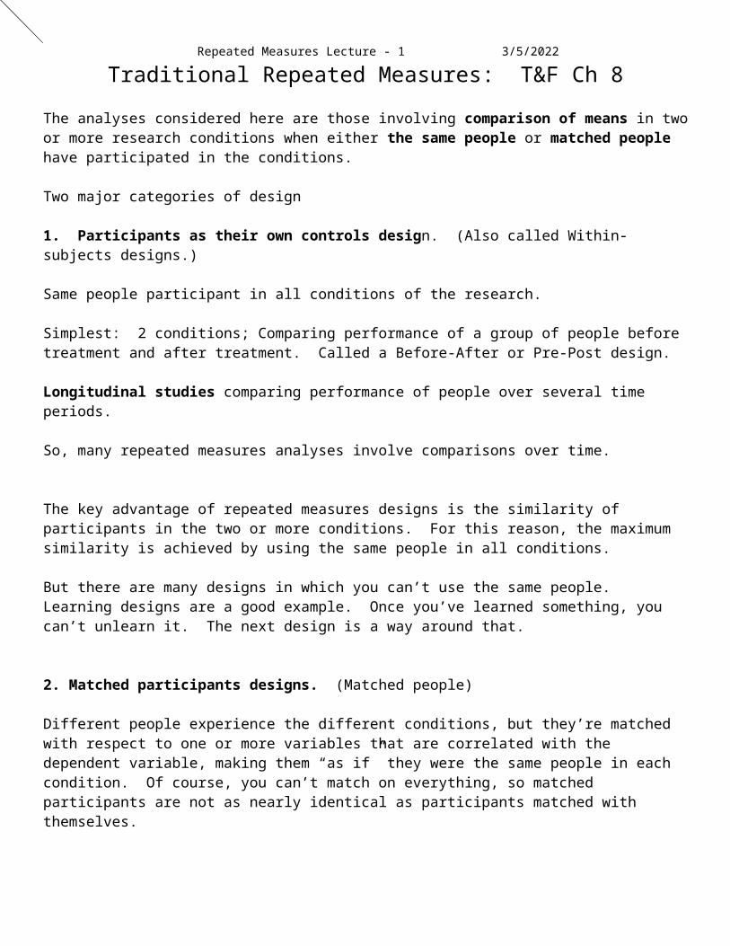
Repeated Measures Lecture - 1 5/7/2023
Traditional Repeated Measures: T&F Ch 8
The analyses considered here are those involving comparison of means in two or more research conditions when either the same people or matched people have participated in the conditions.
Two major categories of design
1. Participants as their own controls design. (Also called Within-subjects designs.)
Same people participant in all conditions of the research.
Simplest: 2 conditions; Comparing performance of a group of people before treatment and after treatment. Called a Before-After or Pre-Post design.
Longitudinal studies comparing performance of people over several time periods.
So, many repeated measures analyses involve comparisons over time.
The key advantage of repeated measures designs is the similarity of participants in the two or more conditions. For this reason, the maximum similarity is achieved by using the same people in all conditions.
But there are many designs in which you can’t use the same people. Learning designs are a good example. Once you’ve learned something, you can’t unlearn it. The next design is a way around that.
2. Matched participants designs. (Matched people)
Different people experience the different conditions, but they’re matched with respect to one or more variables that are correlated with the dependent variable, making them “as if” they were the same people in each condition. Of course, you can’t match on everything, so matched participants are not as nearly identical as participants matched with themselves.
3. Cloned participants designs!!!!!??? (Totally matched organisms)
Having your cake and eating it to. This is a way of having nearly perfectly matched participants without having to use the same people in all conditions. The ultimate matching.

Repeated Measures Lecture - 2 5/7/2023Advantages of Repeated Measures designs
1. Eliminating Confounds. In Between-Subjects designs, an extraneous variable may affect one group, but not the other, creating a confound. Within-Subjects designs are largely free of such confounds from extraneous variables. Since the people in each condition are the same or are matched, differences found between conditions are more likely to be due to treatment differences rather than to participant differences on variables we’re not interested in.
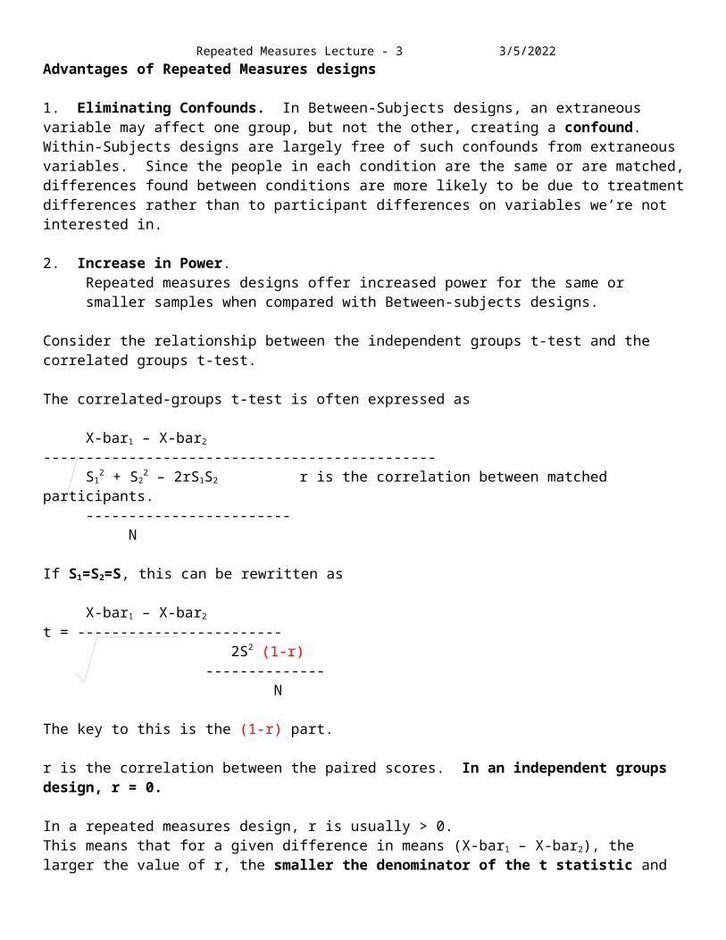
2. Increase in Power.Repeated measures designs offer increased power for the same or smaller samples when compared with Between-subjects designs.
Consider the relationship between the independent groups t-test and the correlated groups t-test.
The correlated-groups t-test is often expressed as
X-bar1 – X-bar2
----------------------------------------------S1
2 + S22 – 2rS1S2 r is the correlation between matched participants.
------------------------N
If S1=S2=S, this can be rewritten as
X-bar1 – X-bar2
t = ------------------------ 2S2 (1-r) -------------- N
The key to this is the (1-r) part.
r is the correlation between the paired scores. In an independent groups design, r = 0.
In a repeated measures design, r is usually > 0.This means that for a given difference in means (X-bar1 – X-bar2), the larger the value of r, the smaller the denominator of the t statistic and therefore the bigger the value of t. The bigger the value of t, the more likely it is to be a rejection t.
That is, power to detect a difference is a positive function of r - the larger the correlation between paired scores, the greater the likelihood of detecting a difference, if there is a difference.
So designs with a positive correlation between scores in the two conditions will be more powerful than designs with zero correlation, e.g., independent groups designs.
Of course, if there is no difference between the means of the two populations, then power is not an issue.
But if there IS a difference between the population mean, the correlated groups design will be more likely to detect it.
Repeated Measures Lecture - 3 5/7/2023 How should data be put in the data editor for repeated measures designs?
Between-subjects Designs: Different conditions are represented in different rows of the data matrix.
Traditional Repeated Measures Designs: Different conditions are represented in different columns of the data matrix with each row representing a person or matched persons.
Condition 1
Condition 2
Condition 1
Condition 2

Lab
T1
Lab
T2
Lab
T3
NoLab
T1
NoLab
T2
NoLab
T3
Repeated Measures Lecture - 4 5/7/2023Data Matrix of Designs with 2 Repeated Measures Factors
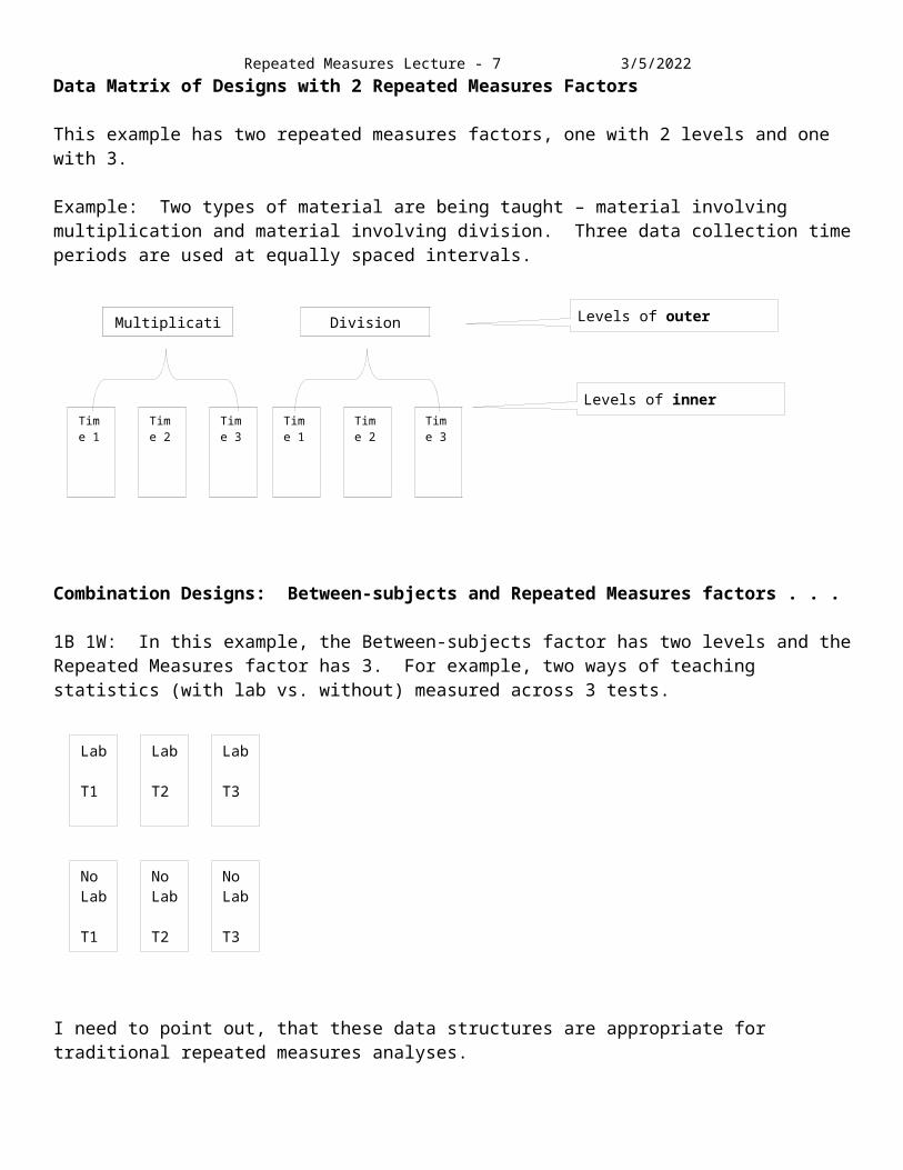
This example has two repeated measures factors, one with 2 levels and one with 3.
Example: Two types of material are being taught – material involving multiplication and material involving division. Three data collection time periods are used at equally spaced intervals.
Combination Designs: Between-subjects and Repeated Measures factors . . .
1B 1W: In this example, the Between-subjects factor has two levels and the Repeated Measures factor has 3. For example, two ways of teaching statistics (with lab vs. without) measured across 3 tests.
I need to point out, that these data structures are appropriate for traditional repeated measures analyses.
Analyses using multilevel modeling procedures require a different data structure. Argh!!
Time 1
Time 2
Time 3
Time 1
Time 2
Time 3
Multiplication Multiplication Division Levels of outer factor
Levels of inner factor

Repeated Measures Lecture - 5 5/7/2023
The simplest type of repeated measures analysis – the paired samples t-test.
Comparing conscientiousness under honest instructions with conscientiousness under faking instructions.The data editor
4.407 – 3.697d = ------------------------ = 1.04 .685
This is a HUGE effect size.

Repeated Measures Lecture - 6 5/7/2023
The paired sample t as an analysis of difference scores.
We’ll get the exact same result by analyzing the single column of f-h difference scores.
Null hypothesis is that the mean of the difference scores is 0.GET FILE='G:\MdbR\0DataFiles\Wrensen_070114.sav'.DATASET NAME DataSet1 WINDOW=FRONT.T-TEST /TESTVAL=0 /MISSING=ANALYSIS /VARIABLES=dcons /CRITERIA=CI(.95).
T-Test[DataSet1] G:\MdbR\0DataFiles\Wrensen_070114.sav
One-Sample Statistics
N Mean Std. Deviation Std. Error Mean
dcons 166 .710 .8431 .0654
One-Sample Test
Test Value = 0
t df Sig. (2-tailed) Mean Difference
95% Confidence Interval of the Difference
Lower Upper
dcons 10.854 165 .000 .7102 .581 .839
From above, for reference . . .
Many statistical procedures involving repeated measures make use of difference scores.
Repeated Measures Lecture - 7 5/7/2023
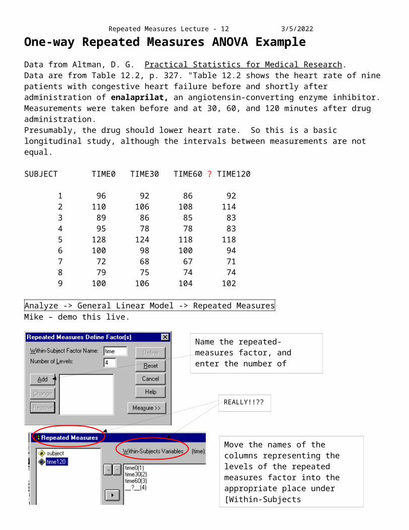
One-way Repeated Measures ANOVA ExampleData from Altman, D. G. Practical Statistics for Medical Research. Data are from Table 12.2, p. 327. "Table 12.2 shows the heart rate of nine patients with congestive heart failure before and shortly after administration of enalaprilat, an angiotensin-converting enzyme inhibitor. Measurements were taken before and at 30, 60, and 120 minutes after drug administration.Presumably, the drug should lower heart rate. So this is a basic longitudinal study, although the intervals between measurements are not equal.
SUBJECT TIME0 TIME30 TIME60 ? TIME120
1 96 92 86 92 2 110 106 108 114 3 89 86 85 83 4 95 78 78 83 5 128 124 118 118 6 100 98 100 94 7 72 68 67 71 8 79 75 74 74 9 100 106 104 102
Analyze -> General Linear Model -> Repeated MeasuresMike – demo this live.
Name the repeated-measures factor, and enter the number of levels. Then click on [Add].
Move the names of the columns representing the levels of the repeated measures factor into the appropriate place under [Within-Subjects Variables]. (Note the change in terminology of the SPSS dialog boxes from Repeated Measures to Within-Subjects.)
REALLY!!???
Repeated Measures Lecture - 8 5/7/2023Using Dummary Variable coding of Time Points
Since the 1st measurement appears to be special, I specified a dummy variable repeated measures contrast in which the all levels were compared with level 1 of the RM factor.
Dummy variable coding is called Simple coding in SPSS.
Since the times are not equally spaced – 30,60,120 – I can’t easily use orthogonal polynomial contrasts to look at the shape of change over time. Drat!!
Check the usual set of optional statistics.
Output for the Parameter Estimates has been erased below, since it was of no value to interpretation of these results.
Plots are a natural adjunct to repeated measures analyses.
Generally speaking you should always make Time the horizontal axis if Time is in your analysis.

Repeated Measures Lecture - 9 5/7/2023The syntax for the analysis.GLM time0 time30 time60 time120 /WSFACTOR = time 4 Simple(1) <<<<---- Specifies the RM factor and the contrast. /METHOD = SSTYPE(3) /PLOT = PROFILE( time ) /PRINT = DESCRIPTIVE ETASQ OPOWER PARAMETER /CRITERIA = ALPHA(.05) /WSDESIGN = time .
General Linear Model
Hypothesis Tested in the Analysis
The null hypothesis that is tested in the analysis can be viewed in two different and essentially equivalent ways.
Version 1 of the Null hypothesis: Equality of Means
The first is that the four means are all equal: H0: µTime0 = µTime30 = µTime60 = µTime120
Version 2 of the Null hypothesis: Means of Differences Equal 0
If the means are all equal then the differences between pairs of means are all 0.
Compute µDiff1 = µTime0 - µTime30
µDiff2 = µTime30 - µTime60 (Any other 3 nonredundant differences would work.)µDiff3 = µTime60 - µTime120
Then the 2nd version of the null hypothesis is: H0: µDiff1 = µDiff2 = µDiff3 = 0
Note that the = 0 at the end of the 2nd null is very important. The null is that every difference is 0.

Repeated Measures Lecture - 10 5/7/2023The Sequence of Tests performed by GLM
The Multivariate test that all mean differences are 0. The first tests performed by GLM are what are called Multivariate Tests. They're called that because they are a test of the hypothesis that the multiple difference variables (3 in our case) are all 0. So, they’re multivariate tests.
Four different multivariate tests are performed. Each is based on slightly different assumptions, and in some instances, the results for the four may be different. In this case, they are all equivalent.
The multivariate tests are the most robust tests of the null hypothesis. This means that they are less affected by nonnormality of the distributions than are the tests that follow. The price paid for that robustness is loss of power. The multivariate tests are less powerful than those that follow. This means that if you're worried about power and are hoping to reject the null, rejecting the null with the multivariate tests means you're home free. But if you fail to reject the null with the multivariate tests, then you have to hope that you meet the restrictions for the more powerful tests that follow.
In this case, we fail to reject the null using the multivariate tests.
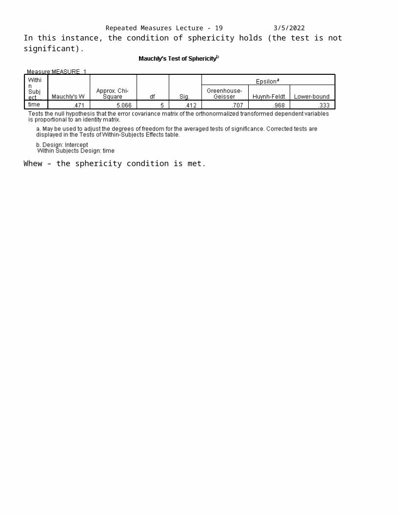
The test of sphericity . When conducting a one-way repeated measures ANOVA, the values of variances and covariances should fall within specific ranges. If this is so, the matrix is said to meet the sphericity criterion. If the sphericity criterion is met, then the most powerful test of the null can be employed. If it not met, then either the multivariate test must be used, or one of the special tests devoted to getting around the failure to find sphericity must be employed. Fortunately, SPSS gives you all the tests, so you can pick the one which is appropriate. The null hypothesis in Mauchly's test is that the sphericity condition holds, so we generally hope to not reject the null.
In this instance, the condition of sphericity holds (the test is not significant).
Whew – the sphericity condition is met.
Repeated Measures Lecture - 11 5/7/2023The Univariate Tests. Since the sphericity condition is met, we can use the test of significance printed in the top line of the following box.
If sphericity didn't hold, then we would either report the multivariate F above or report one of the F's from the 2nd, 3rd, or 4th lines of the table below. Each of them performs an adjustment for lack of sphericity. The specifics of the adjustment vary across tests. Note that in the top three lines, the null is rejected. The last line reports the most conservative adjustment. But since sphericity holds, we can report the F in the top line and conclude that there are significant differences between mean heart rates across time periods.The difference between these results and those of the Multivariate tests shown above highlight the power differences between the two types of tests. If you want to detect small differences, use the tests shown below.
Tests of user-specified Contrasts The following tests are of the contrasts specified above on page 8. If no contrasts had been specified, it would not be printed. The individual contrasts compare the means of the 30-, 60-, and 120-minute measurements with the pre-measure. The means at the 60- and 120-minute intervals were significantly lower than the pre-measure mean as we might expect if it took time for the drug to take effect.
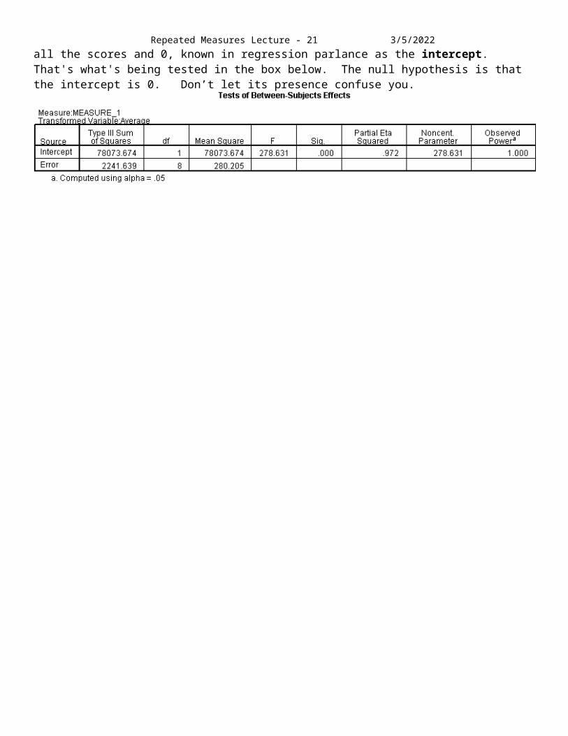
Tests of Between-Subjects Effects. What are between-subjects factors doing in a repeated measures analysis? The answer is that there is only a technical between-subjects factor here - the difference between the mean of all the scores and 0, known in regression parlance as the intercept. That's what's being tested in the box below. The null hypothesis is that the intercept is 0. Don’t let its presence confuse you.
Repeated Measures Lecture - 12 5/7/2023
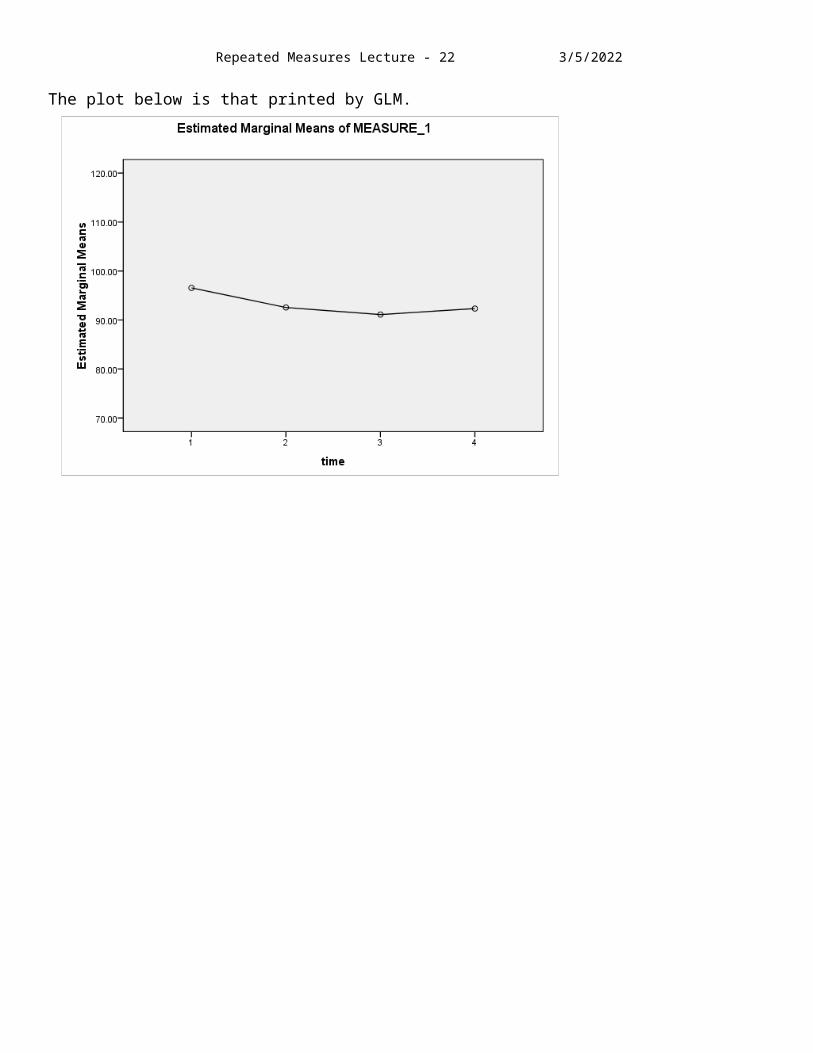
The plot below is that printed by GLM.

Repeated Measures Lecture - 13 5/7/2023
Repeated Measures Profile AnalysisA 2 x 5 Repeated Measures Analysis
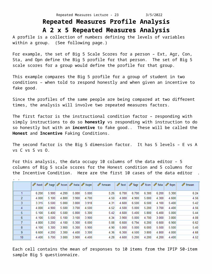
A profile is a collection of numbers defining the levels of variables within a group. (See following page.)
For example, the set of Big 5 Scale Scores for a person – Ext, Agr, Con, Sta, and Opn define the Big 5 profile for that person. The set of Big 5 scale scores for a group would define the profile for that group.
This example compares the Big 5 profile for a group of student in two conditions – when told to respond honestly and when given an incentive to fake good.
Since the profiles of the same people are being compared at two different times, the analysis will involve two repeated measures factors.
The first factor is the instructional condition factor – responding with simply instructions to do so honestly vs responding with instruction to do so honestly but with an incentive to fake good.. These will be called the Honest and Incentive Faking Conditions.
The second factor is the Big 5 dimension factor. It has 5 levels – E vs A vs C vs S vs O.
For this analysis, the data occupy 10 columns of the data editor – 5 columns of Big 5 scale scores for the Honest condition and 5 columns for the Incentive Condition. Here are the first 10 cases of the data editor . . .
Each cell contains the mean of responses to 10 items from the IPIP 50-item sample Big 5 questionnaire.
In the analysis, three major comparisons will be made . . .
1. The main effect of Faking Conditon – Mean of all responses in the Honest vs. Mean of all in the Incentive condition.
2. The main effect of Big 5 dimension – Mean of all responses in to Ext items vs mean of Agr items vs. mean of Con items vs mean of Sta items vs mean of Opn items.
3. The interaction of Faking Conditon and Big 5 Dimensions - A comparison of differences in hones and incentive in Ext vs the difference in Agr vs the difference in Con vs the differnce in Sta vs the difference in Opn.

Repeated Measures Lecture - 14 5/7/2023GET FILE='G:\MDBR\0DataFiles\IncentiveData110923 w wpt 150416.sav'.DATASET NAME DataSet2 WINDOW=FRONT.DATASET ACTIVATE DataSet2.DATASET CLOSE DataSet1.
Profile of New York building heights

Repeated Measures Lecture - 15 5/7/2023
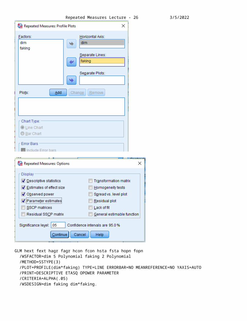
GLM hext fext hagr fagr hcon fcon hsta fsta hopn fopn /WSFACTOR=dim 5 Polynomial faking 2 Polynomial /METHOD=SSTYPE(3) /PLOT=PROFILE(dim*faking) TYPE=LINE ERRORBAR=NO MEANREFERENCE=NO YAXIS=AUTO /PRINT=DESCRIPTIVE ETASQ OPOWER PARAMETER /CRITERIA=ALPHA(.05) /WSDESIGN=dim faking dim*faking.

Repeated Measures Lecture - 16 5/7/2023General Linear Model
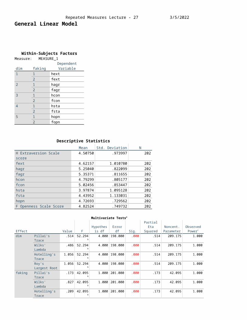
Within-Subjects FactorsMeasure: MEASURE_1
dim fakingDependent
Variable1 1 hext
2 fext2 1 hagr
2 fagr3 1 hcon
2 fcon4 1 hsta
2 fsta5 1 hopn
2 fopn
Descriptive StatisticsMean Std. Deviation N
H Extraversion Scale score 4.50750 .973997 202fext 4.62157 1.010780 202hagr 5.25040 .822099 202fagr 5.35371 .811655 202hcon 4.79299 .805177 202fcon 5.02456 .853447 202hsta 3.97874 1.095128 202fsta 4.43952 1.133031 202hopn 4.72693 .729562 202F Openness Scale Score 4.82524 .749732 202
Multivariate Testsa
Effect Value FHypothesis
df Error df Sig.Partial Eta Squared
Noncent. Parameter
Observed Powerc
dim Pillai's Trace .514 52.294b 4.000 198.000 .000 .514 209.175 1.000Wilks' Lambda .486 52.294b 4.000 198.000 .000 .514 209.175 1.000Hotelling's Trace 1.056 52.294b 4.000 198.000 .000 .514 209.175 1.000Roy's Largest Root
1.056 52.294b 4.000 198.000 .000 .514 209.175 1.000
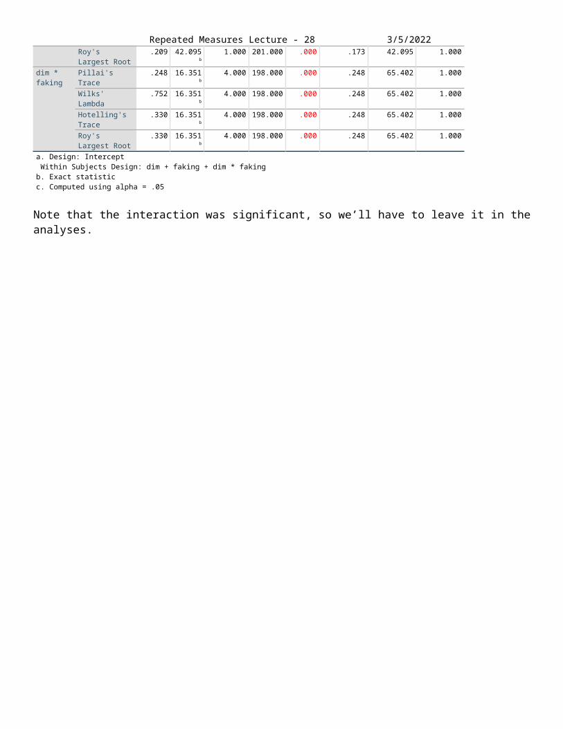
faking Pillai's Trace .173 42.095b 1.000 201.000 .000 .173 42.095 1.000Wilks' Lambda .827 42.095b 1.000 201.000 .000 .173 42.095 1.000Hotelling's Trace .209 42.095b 1.000 201.000 .000 .173 42.095 1.000Roy's Largest Root
.209 42.095b 1.000 201.000 .000 .173 42.095 1.000
dim * faking
Pillai's Trace .248 16.351b 4.000 198.000 .000 .248 65.402 1.000Wilks' Lambda .752 16.351b 4.000 198.000 .000 .248 65.402 1.000Hotelling's Trace .330 16.351b 4.000 198.000 .000 .248 65.402 1.000Roy's Largest Root
.330 16.351b 4.000 198.000 .000 .248 65.402 1.000
a. Design: Intercept Within Subjects Design: dim + faking + dim * fakingb. Exact statisticc. Computed using alpha = .05
Note that the interaction was significant, so we’ll have to leave it in the analyses.

Repeated Measures Lecture - 17 5/7/2023
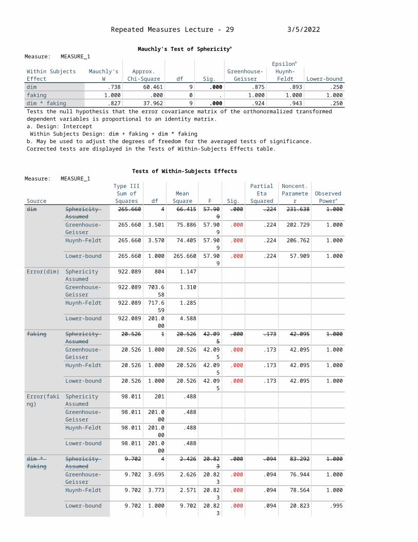
Mauchly's Test of Sphericitya
Measure: MEASURE_1
Within Subjects Effect Mauchly's WApprox. Chi-
Square df Sig.
Epsilonb
Greenhouse-Geisser Huynh-Feldt Lower-bound
dim .738 60.461 9 .000 .875 .893 .250faking 1.000 .000 0 . 1.000 1.000 1.000dim * faking .827 37.962 9 .000 .924 .943 .250Tests the null hypothesis that the error covariance matrix of the orthonormalized transformed dependent variables is proportional to an identity matrix.a. Design: Intercept Within Subjects Design: dim + faking + dim * fakingb. May be used to adjust the degrees of freedom for the averaged tests of significance. Corrected tests are displayed in the Tests of Within-Subjects Effects table.
Tests of Within-Subjects EffectsMeasure: MEASURE_1
Source
Type III Sum of Squares df
Mean Square F Sig.
Partial Eta Squared
Noncent. Parameter
Observed Powera
dim Sphericity Assumed
265.660 4 66.415 57.909 .000 .224 231.638 1.000
Greenhouse-Geisser
265.660 3.501 75.886 57.909 .000 .224 202.729 1.000
Huynh-Feldt 265.660 3.570 74.405 57.909 .000 .224 206.762 1.000Lower-bound 265.660 1.000 265.660 57.909 .000 .224 57.909 1.000
Error(dim) Sphericity Assumed
922.089 804 1.147
Greenhouse-Geisser
922.089 703.658
1.310
Huynh-Feldt 922.089 717.659
1.285
Lower-bound 922.089 201.000
4.588
faking Sphericity Assumed
20.526 1 20.526 42.095 .000 .173 42.095 1.000
Greenhouse-Geisser
20.526 1.000 20.526 42.095 .000 .173 42.095 1.000
Huynh-Feldt 20.526 1.000 20.526 42.095 .000 .173 42.095 1.000Lower-bound 20.526 1.000 20.526 42.095 .000 .173 42.095 1.000
Error(faking) Sphericity Assumed
98.011 201 .488
Greenhouse-Geisser
98.011 201.000
.488
Huynh-Feldt 98.011 201.000
.488
Lower-bound 98.011 201.000
.488
dim * faking Sphericity Assumed
9.702 4 2.426 20.823 .000 .094 83.292 1.000
Greenhouse-Geisser
9.702 3.695 2.626 20.823 .000 .094 76.944 1.000
Huynh-Feldt 9.702 3.773 2.571 20.823 .000 .094 78.564 1.000Lower-bound 9.702 1.000 9.702 20.823 .000 .094 20.823 .995
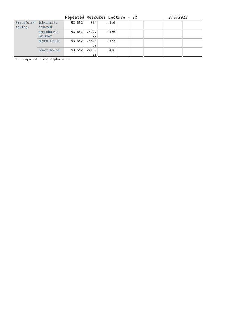
Error(dim*faking)
Sphericity Assumed
93.652 804 .116
Greenhouse-Geisser
93.652 742.722
.126
Huynh-Feldt 93.652 758.359
.123
Lower-bound 93.652 201.000
.466
a. Computed using alpha = .05

Repeated Measures Lecture - 18 5/7/2023
Tests of Within-Subjects ContrastsMeasure: MEASURE_1
Source dim faking
Type III Sum of
Squares dfMean
Square F Sig.Partial Eta Squared
Noncent. Parameter
Observed Powera
dim Linear 18.126 1 18.126 15.944 .000 .073 15.944 .978Quadratic
12.098 1 12.098 10.839 .001 .051 10.839 .906
Cubic 232.202 1 232.202 171.318
.000 .460 171.318 1.000
Order 4 3.234 1 3.234 3.303 .071 .016 3.303 .440Error(dim) Linear 228.514 201 1.137
Quadratic
224.359 201 1.116
Cubic 272.432 201 1.355Order 4 196.785 201 .979
faking Linear
20.526 1 20.526 42.095 .000 .173 42.095 1.000
Error(faking) Linear
98.011 201 .488
dim * faking Linear Linear
1.073 1 1.073 10.434 .001 .049 10.434 .895
Quadratic
Linear
2.618 1 2.618 22.292 .000 .100 22.292 .997
Cubic Linear
5.392 1 5.392 42.427 .000 .174 42.427 1.000
Order 4 Linear
.618 1 .618 5.215 .023 .025 5.215 .623
Error(dim*faking)
Linear Linear
20.673 201 .103
Quadratic
Linear
23.610 201 .117
Cubic Linear
25.547 201 .127
Order 4 Linear
23.822 201 .119
a. Computed using alpha = .05
Tests of Between-Subjects EffectsMeasure: MEASURE_1Transformed Variable: Average
SourceType III Sum of Squares df Mean Square F Sig.
Partial Eta Squared
Noncent. Parameter
Observed Powera
Intercept 45616.886 1 45616.886 16783.070 .000 .988 16783.070 1.000Error 546.324 201 2.718a. Computed using alpha = .05
There were no quantitative differences between Big 5 dimensions, so orthogonal polynomial contrasts are not appropriate.
Repeated Measures Lecture - 19 5/7/2023
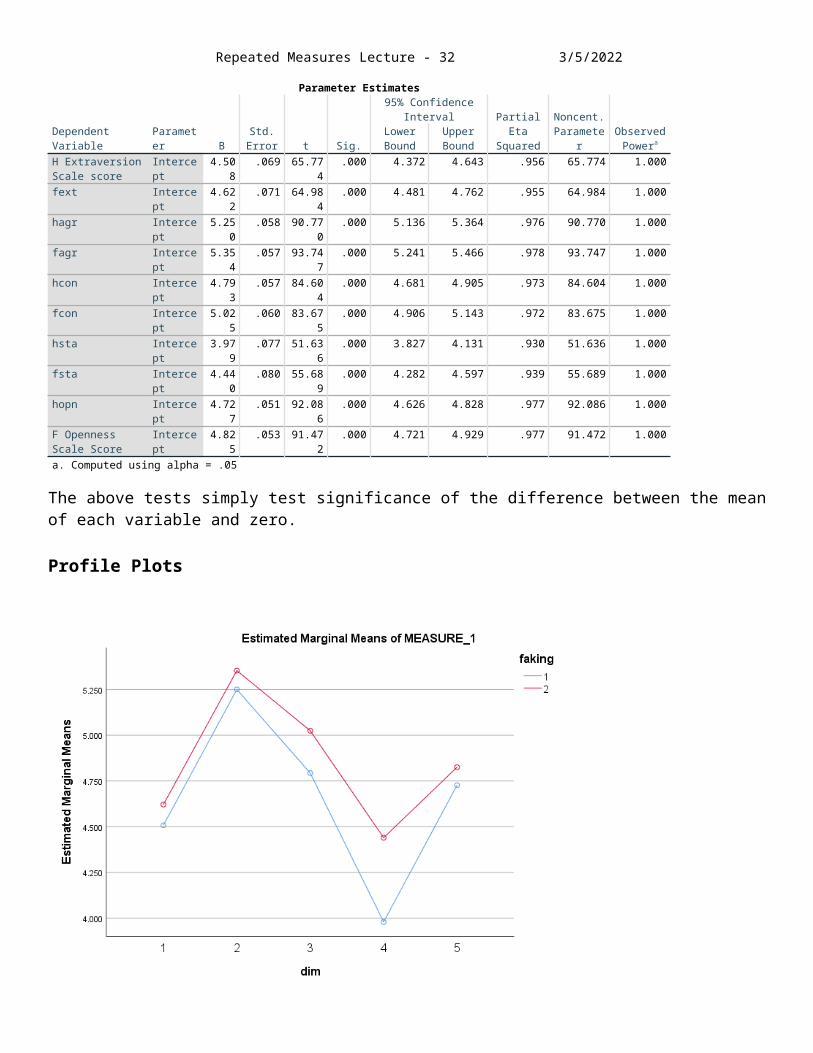
Parameter Estimates
Dependent Variable
Parameter B
Std. Error t Sig.
95% Confidence Interval
Partial Eta Squared
Noncent. Parameter
Observed Powera
Lower Bound
Upper Bound
H Extraversion Scale score
Intercept 4.508 .069 65.774 .000 4.372 4.643 .956 65.774 1.000
fext Intercept 4.622 .071 64.984 .000 4.481 4.762 .955 64.984 1.000hagr Intercept 5.250 .058 90.770 .000 5.136 5.364 .976 90.770 1.000fagr Intercept 5.354 .057 93.747 .000 5.241 5.466 .978 93.747 1.000hcon Intercept 4.793 .057 84.604 .000 4.681 4.905 .973 84.604 1.000fcon Intercept 5.025 .060 83.675 .000 4.906 5.143 .972 83.675 1.000hsta Intercept 3.979 .077 51.636 .000 3.827 4.131 .930 51.636 1.000fsta Intercept 4.440 .080 55.689 .000 4.282 4.597 .939 55.689 1.000hopn Intercept 4.727 .051 92.086 .000 4.626 4.828 .977 92.086 1.000F Openness Scale Score
Intercept 4.825 .053 91.472 .000 4.721 4.929 .977 91.472 1.000
a. Computed using alpha = .05
The above tests simply test significance of the difference between the mean of each variable and zero.
Profile Plots
Respondents gave more positive responses to all dimensions in the Incentive condition.
There were significant differences in mean response to the Five dimensions.
The effect of Incentive was greater for Dimensions 3 (Conscientiousness) and 4 (Stability).
HonestIncentive

Bridge Group
Control Group
Repeated Measures Lecture - 20 5/7/2023
Repeated Measures ANOVA – start here on 10/16/171 Between Groups Factor / 1 Repeated Measures Factor
The Learning to Play Bridge effectiveness study.
Situation: A school system provides middle and high school students a period for whatever intellectual activity they wish to engage in. Some choose chess; some choose reading, some choose programming, some choose to play the card game called bridge.
One of the people involved with the bridge classes was interested in whether playing bridge during the hour periods over a long period of time would lead to greater performance on standardized tests of school-related achievement than the other activities. The data here provide a test of that notion.
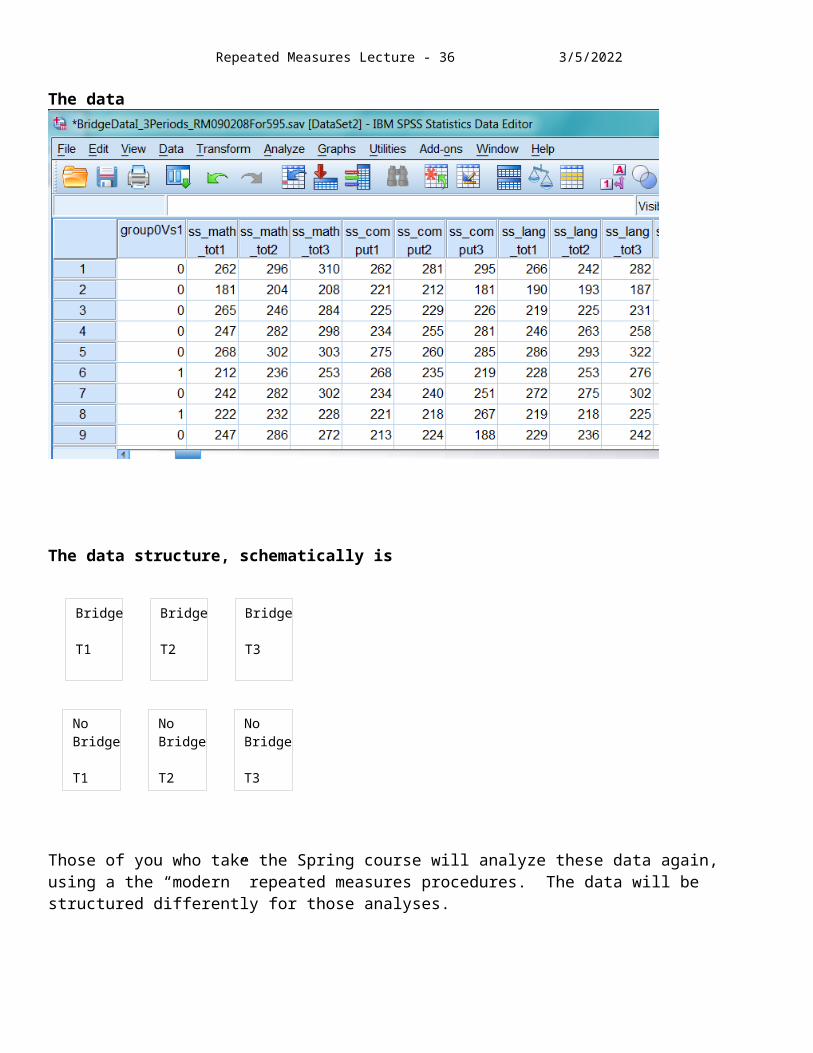
File: BridgeData1_3Periods_RM090208For595.sav
Key variables:
group0Vs1. Variable representing the research condition. 0=Control; 1=Bridge
ss_math_tot1 ss_math_tot2 ss_math_tot3 Standardized total scores on math achievement at time period 1, time period 2 and time period 3.
ss_comput1 ss_comput2 ss_comput3: Standardized “computational??” achievement
ss_lang_tot1 ss_lang_tot2 ss_lang_tot3: Standardized language achievement
(The names of the variables are idiosyncratic because of the way the data were given to me. I’ve just been too lazy to change them to something easier to follow.)
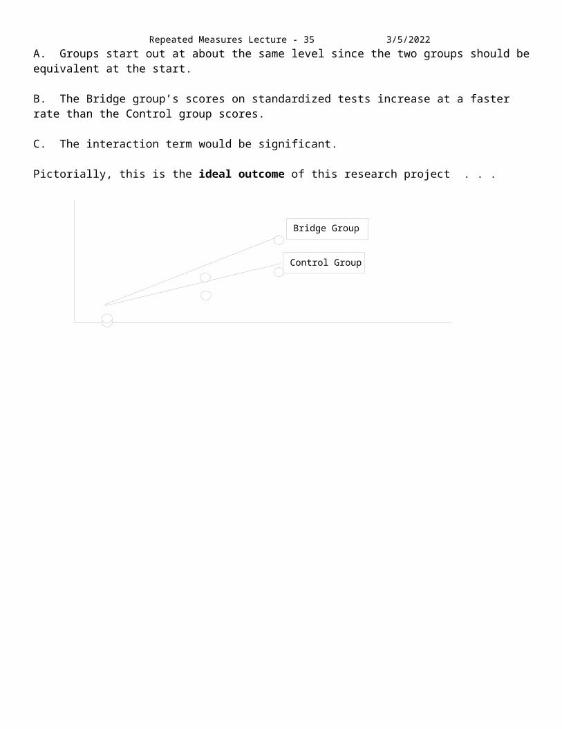
What outcome would be ideal here??
A. Groups start out at about the same level since the two groups should be equivalent at the start.
B. The Bridge group’s scores on standardized tests increase at a faster rate than the Control group scores.
C. The interaction term would be significant.
Pictorially, this is the ideal outcome of this research project . . .
Bridge
T1
Bridge
T2
Bridge
T3
NoBridge
T1
NoBridge
T2
NoBridge
T3
Repeated Measures Lecture - 21 5/7/2023
The data
The data structure, schematically is
Those of you who take the Spring course will analyze these data again, using a the “modern” repeated measures procedures. The data will be structured differently for those analyses.
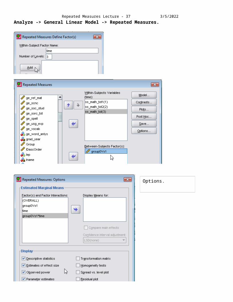
Repeated Measures Lecture - 22 5/7/2023Analyze -> General Linear Model -> Repeated Measures.
Options.
Repeated Measures Lecture - 23 5/7/2023
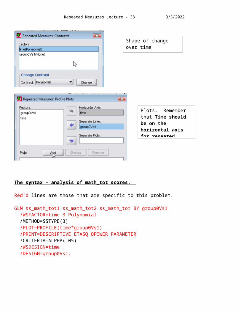
The syntax – analysis of math_tot scores.
Red’d lines are those that are specific to this problem.
GLM ss_math_tot1 ss_math_tot2 ss_math_tot BY group0Vs1 /WSFACTOR=time 3 Polynomial /METHOD=SSTYPE(3) /PLOT=PROFILE(time*group0Vs1) /PRINT=DESCRIPTIVE ETASQ OPOWER PARAMETER /CRITERIA=ALPHA(.05) /WSDESIGN=time /DESIGN=group0Vs1.
Shape of change over time
Plots. Remember that Time should be on the horizontal axis for repeated measures designs.
Repeated Measures Lecture - 24 5/7/2023
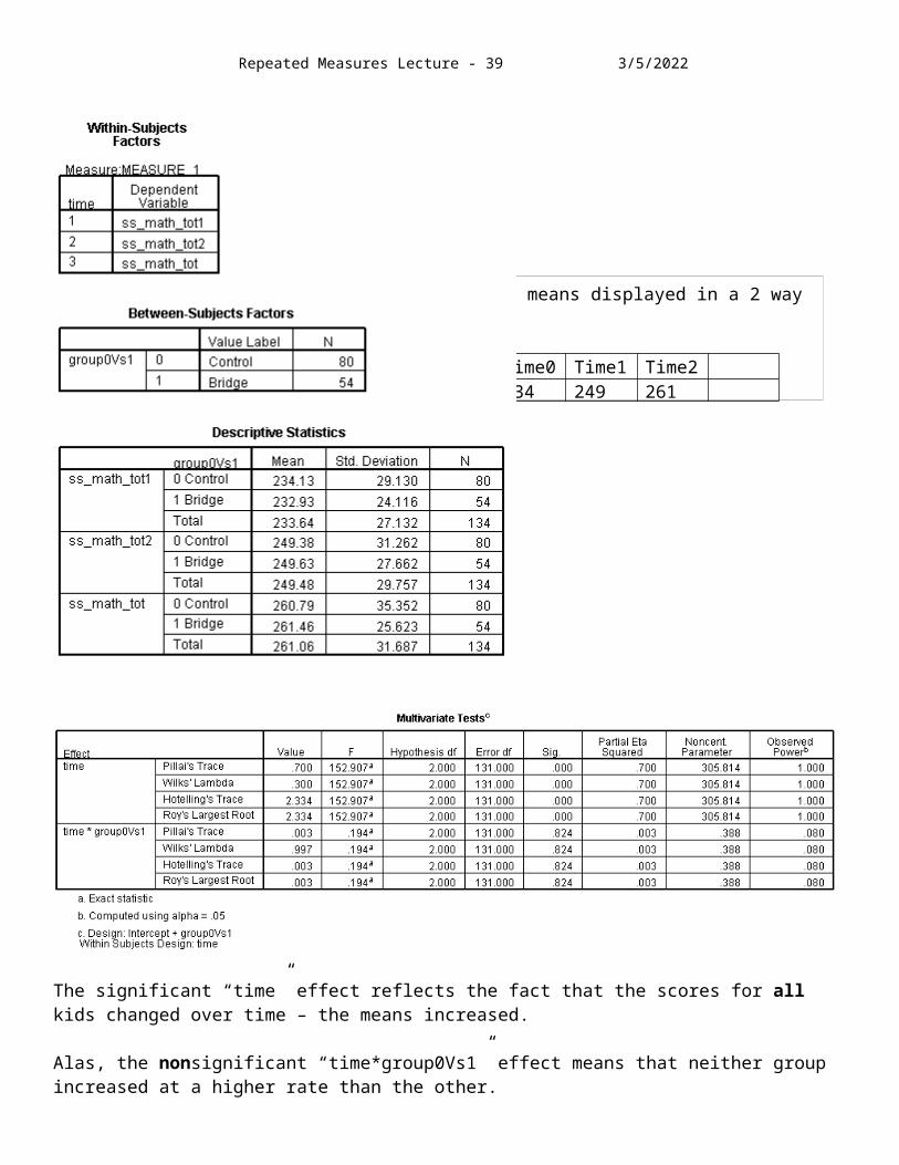
The significant “time” effect reflects the fact that the scores for all kids changed over time – the means increased.
Alas, the nonsignificant “time*group0Vs1” effect means that neither group increased at a higher rate than the other.
The cell means displayed in a 2 way table
Group Time0 Time1 Time2Control 234 249 261Bridge 233 250 261

Repeated Measures Lecture - 25 5/7/2023
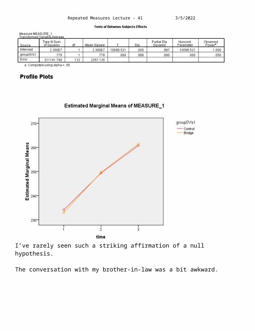
There is a Between-subjects effect in this analysis – the Bridge group vs Control group factor. The table below presents a test of the significance of difference between the overall mean of the Bridge group scores vs the overall mean of the Control group scores. The difference is not significant.
Repeated Measures Lecture - 26 5/7/2023
I’ve rarely seen such a striking affirmation of a null hypothesis.
The conversation with my brother-in-law was a bit awkward.
Repeated Measures Lecture - 27 5/7/2023 Policy Capturing using – skip in 2017
Repeated Measures Analyses
Those in the I-O program know that cognitive ability is the single best predictor of performance in a variety of situations, including academia.
Although we know that cognitive ability is a valid predictor, it’s possible that others do not have that knowledge. If those others are involved in selection of employees, that lack of knowledge could be a serious problem for the organization at which they are employed.
This is a hypothetical research project to investigate whether or not HR persons involved in selection understand these basic results. It uses a technique called policy capturing. In policy capturing, persons are given scenarios and asked to rate each scenario on one or more dimensions. The scenarios are created so that they differ in specific ways, although the raters are not told about these differences. After the ratings have been gathered, analyses of the ratings are conducted to determine if the differences in the scenarios affected the ratings. If the raters had specific, perhaps hidden, policies controlling their ratings of the scenarios, e.g., prejudice against Blacks or females, those policies would be revealed by differences in ratings of the different subgroups distinguished by the characteristics impacted by the policies.
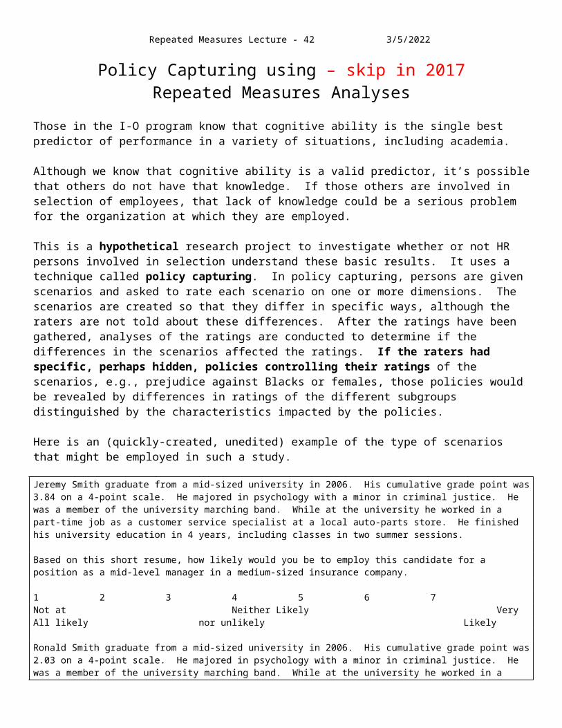
Here is an (quickly-created, unedited) example of the type of scenarios that might be employed in such a study.
Jeremy Smith graduate from a mid-sized university in 2006. His cumulative grade point was 3.84 on a 4-point scale. He majored in psychology with a minor in criminal justice. He was a member of the university marching band. While at the university he worked in a part-time job as a customer service specialist at a local auto-parts store. He finished his university education in 4 years, including classes in two summer sessions.
Based on this short resume, how likely would you be to employ this candidate for a position as a mid-level manager in a medium-sized insurance company.
1 2 3 4 5 6 7Not at Neither Likely VeryAll likely nor unlikely Likely
Ronald Smith graduate from a mid-sized university in 2006. His cumulative grade point was 2.03 on a 4-point scale. He majored in psychology with a minor in criminal justice. He was a member of the university marching band. While at the university he worked in a part-time job as a customer service specialist at a local auto-parts store. He finished his university education in 4 years, including classes in two summer sessions.
Based on this short resume, how likely would you be to employ this candidate for a position as a mid-level manager in a medium-sized insurance company.
1 2 3 4 5 6 7Not at Neither Likely VeryAll likely nor unlikely Likely
Obviously, more than two such scenarios would have to be included in the questionnaire and the two scenarios would have to be less similar in wording than the examples above. Several “high cognitive ability” scenarios might be presented with differently-names participants as well as several “low cognitive ability” scenarios.
Repeated Measures Lecture - 28 5/7/2023In this example, the dependent variable, the ratings, will be of suitability for employment. Let’s suppose that we have a four-item scale of suitability, with reliability = .8. (The above examples give only one of the four items in the scale.)
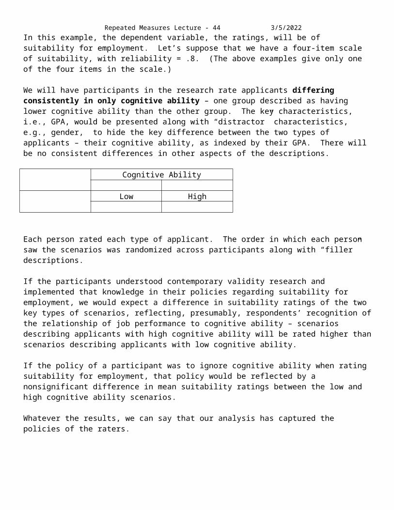
We will have participants in the research rate applicants differing consistently in only cognitive ability – one group described as having lower cognitive ability than the other group. The key characteristics, i.e., GPA, would be presented along with “distractor” characteristics, e.g., gender, to hide the key difference between the two types of applicants – their cognitive ability, as indexed by their GPA. There will be no consistent differences in other aspects of the descriptions.
Cognitive Ability
Low High
Each person rated each type of applicant. The order in which each person saw the scenarios was randomized across participants along with “filler” descriptions.
If the participants understood contemporary validity research and implemented that knowledge in their policies regarding suitability for employment, we would expect a difference in suitability ratings of the two key types of scenarios, reflecting, presumably, respondents’ recognition of the relationship of job performance to cognitive ability – scenarios describing applicants with high cognitive ability will be rated higher than scenarios describing applicants with low cognitive ability.
If the policy of a participant was to ignore cognitive ability when rating suitability for employment, that policy would be reflected by a nonsignificant difference in mean suitability ratings between the low and high cognitive ability scenarios.
Whatever the results, we can say that our analysis has captured the policies of the raters.
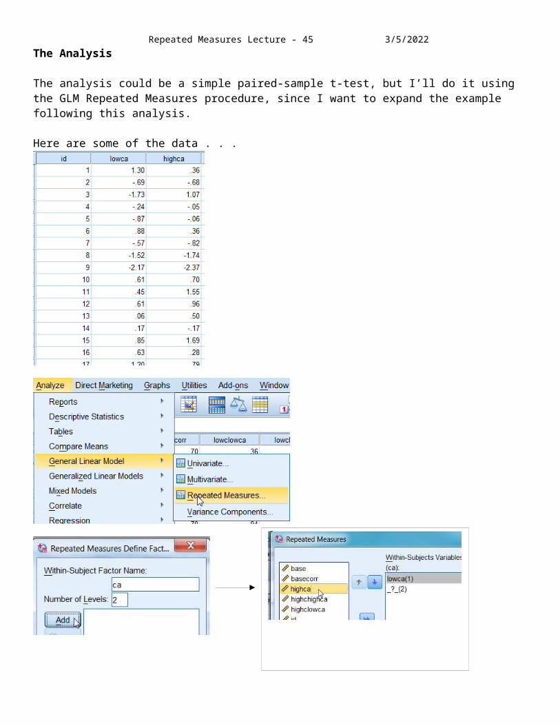
Repeated Measures Lecture - 29 5/7/2023The Analysis
The analysis could be a simple paired-sample t-test, but I’ll do it using the GLM Repeated Measures procedure, since I want to expand the example following this analysis.
Here are some of the data . . .
Repeated Measures Lecture - 30 5/7/2023
General Linear Model
NotesOutput Created 23-SEP-2015 10:18:01Comments
Input Filter <none>Weight <none>Split File <none>N of Rows in Working Data File 80
Missing Value Handling Definition of Missing User-defined missing values are treated as missing.Cases Used Statistics are based on all cases with valid data for all variables in
the model.Syntax GLM lowca highca
/WSFACTOR=ca 2 Polynomial /METHOD=SSTYPE(3) /PLOT=PROFILE(ca) /PRINT=DESCRIPTIVE ETASQ OPOWER /CRITERIA=ALPHA(.05) /WSDESIGN=ca.
Resources Processor Time 00:00:00.14Elapsed Time 00:00:00.14
Within-Subjects FactorsMeasure: MEASURE_1ca Dependent Variable1 lowca2 highca

Repeated Measures Lecture - 31 5/7/2023
Descriptive Statistics
Mean Std. Deviation Nlowca .1536 .91630 80highca .4583 .86124 80
Multivariate Testsa
Effect Value F Hypothesis df Error df Sig.Partial Eta Squared
Noncent. Parameter
Observed Powerc
ca Pillai's Trace .176 16.872b 1.000 79.000 .000 .176 16.872 .982Wilks' Lambda .824 16.872b 1.000 79.000 .000 .176 16.872 .982Hotelling's Trace .214 16.872b 1.000 79.000 .000 .176 16.872 .982Roy's Largest Root .214 16.872b 1.000 79.000 .000 .176 16.872 .982
a. Design: Intercept Within-subjects Design: cab. Exact statisticc. Computed using alpha = .05
Mauchly's Test of Sphericitya
Measure: MEASURE_1
Within-subjects Effect Mauchly's WApprox. Chi-
Square df Sig.
Epsilonb
Greenhouse-Geisser Huynh-Feldt Lower-bound
ca 1.000 .000 0 . 1.000 1.000 1.000Tests the null hypothesis that the error covariance matrix of the orthonormalized transformed dependent variables is proportional to an identity matrix.a. Design: Intercept Within-subjects Design: cab. May be used to adjust the degrees of freedom for the averaged tests of significance. Corrected tests are displayed in the Tests of Within-Subjects Effects table.
Tests of Within-Subjects EffectsMeasure: MEASURE_1
SourceType III Sum of Squares df Mean Square F Sig.
Partial Eta Squared
Noncent. Parameter
Observed Powera
ca Sphericity Assumed 3.714 1 3.714 16.872 .000 .176 16.872 .982Greenhouse-Geisser 3.714 1.000 3.714 16.872 .000 .176 16.872 .982Huynh-Feldt 3.714 1.000 3.714 16.872 .000 .176 16.872 .982Lower-bound 3.714 1.000 3.714 16.872 .000 .176 16.872 .982
Error(ca) Sphericity Assumed 17.390 79 .220
Greenhouse-Geisser 17.390 79.000 .220
Huynh-Feldt 17.390 79.000 .220
Lower-bound 17.390 79.000 .220
a. Computed using alpha = .05
Tests of Within-Subjects ContrastsMeasure: MEASURE_1
Source caType III Sum of
Squares df Mean Square F Sig.Partial Eta Squared
Noncent. Parameter
Observed Powera
ca Linear 3.714 1 3.714 16.872 .000 .176 16.872 .982Error(ca) Linear 17.390 79 .220
a. Computed using alpha = .05
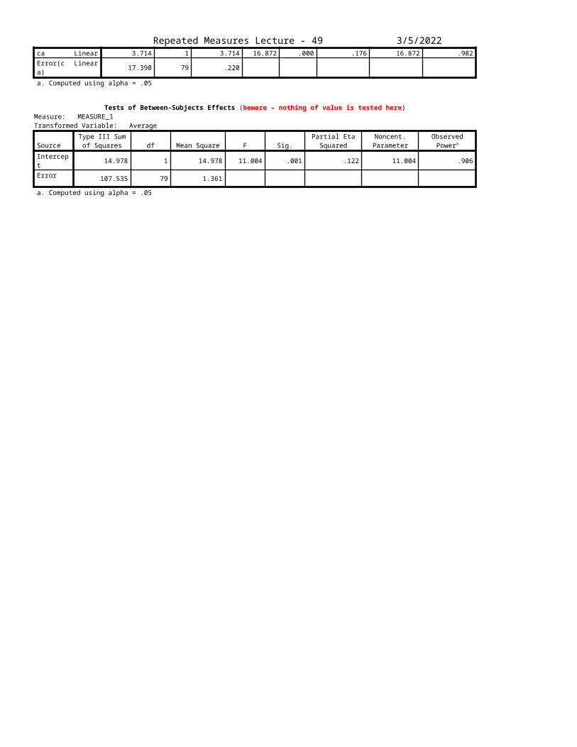
Tests of Between-Subjects Effects (beware – nothing of value is tested here)Measure: MEASURE_1Transformed Variable: Average
SourceType III Sum of
Squares df Mean Square F Sig.Partial Eta Squared
Noncent. Parameter Observed Powera
Intercept 14.978 1 14.978 11.004 .001 .122 11.004 .906Error 107.535 79 1.361
a. Computed using alpha = .05
Mauchly’s test is not applicable when the repeated measures factor has only 2 levels.
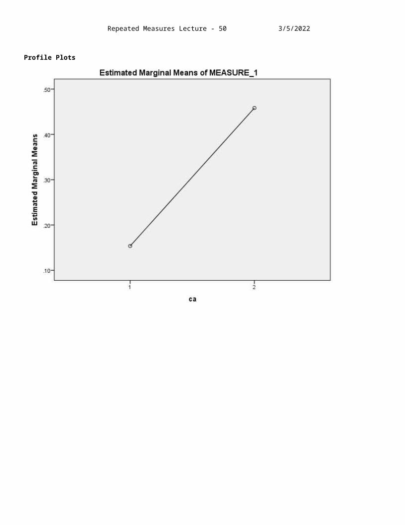
Repeated Measures Lecture - 32 5/7/2023
Profile Plots

Repeated Measures Lecture - 33 5/7/2023
Policy Capturing usingFactorial Repeated Measures
(Pardon the repetition from the previous example.)
Those in the I-O program know that cognitive ability is the single best predictor of performance in a variety of situations, including academia. Many also know that conscientiousness is also a valid, though less efficacious predictor of performance, also including performance in academia.
Although we know that these two characteristics are valid predictors, it’s possible that others do not have that knowledge. If those others are involved in selection of employees, that could be a serious problem for the organization at which they are employed.
This is a hypothetical research project to investigate whether or not HR persons involved in selection understand these basic results. It uses a technique called policy capturing. In policy capturing, persons are given scenarios and asked to rate each scenario on one or more dimensions. The scenarios are created so that they differ in specific ways, although the raters are not told about these differences. After the ratings have been gathered, analyses of the ratings are conducted to determine if the differences in the scenarios affected the ratings. If the raters had specific policies regarding the differences in the scenarios, e.g., prejudice against Blacks or females, those policies would be revealed by differences in ratings of the different subgroups distinguished by those policies.
In this example, the dependent variable, the ratings, will be of suitability for employement. Let’s suppose that we have a four-item scale of suitability, with reliability = .8.
We will have persons rate four different types of hypothetical applicant. The four types of applicants will be described as having different combinations of cognitive ability and conscientiousness – four combinations arranged factorially as shown in the following table . . .
Low Cons Low Consc High Consc High ConscRespondent Low CA High CA Low CA High CA
12
Assume that the order in which each person saw the scenarios was randomized across participants. Don’t ask me for examples of the scenarios. That would be a difficult, though I believe achievable task.
If the participants understood contemporary validity research, we would expect
1. A positive relationship of suitability to cognitive ability – scenarios describing applicants with high cognitive ability will be rated higher than scenarios describing applicants with low cognitive ability.2. A positive relationship of suitability to conscientiousness – scenarios describing applicants with high conscientiousness will be rated higher than scenarios describing applicants with low conscientiousness.3. No interaction between the effects of cognitive ability and conscientiousness on ratings – the effect of cognitive ability will be the same across conscientiousness levels and the effect of conscientiousness will be the same across levels of cognitive ability.

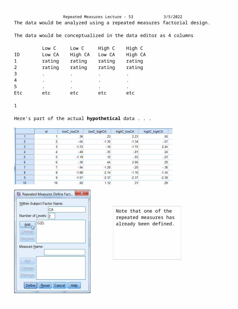
Repeated Measures Lecture - 34 5/7/2023The data would be analyzed using a repeated measures factorial design.
The data would be conceptualized in the data editor as 4 columns
Low C Low C High C High CID Low CA High CA Low CA High CA1 rating rating rating rating2 rating rating rating rating3 . . . .4 . . . .5 . . . .Etc etc etc etc etc
1
Here’s part of the actual hypothetical data . . .
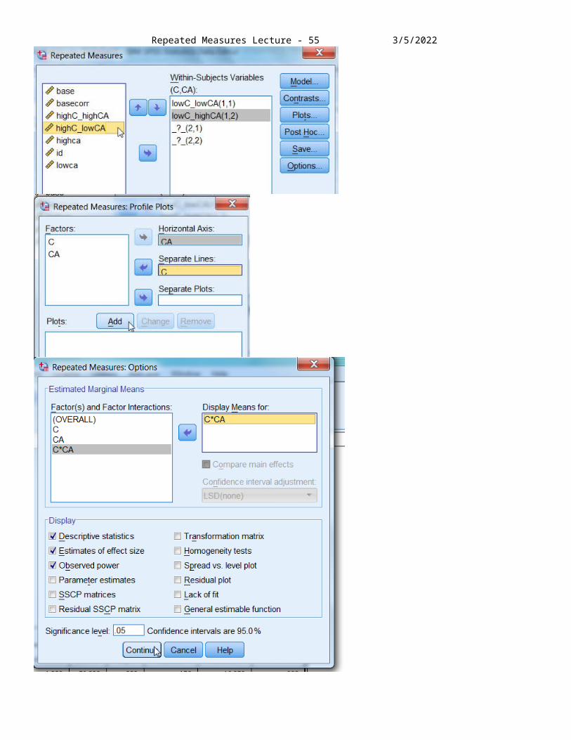
Note that one of the repeated measures has already been defined.
Repeated Measures Lecture - 35 5/7/2023
Repeated Measures Lecture - 36 5/7/2023
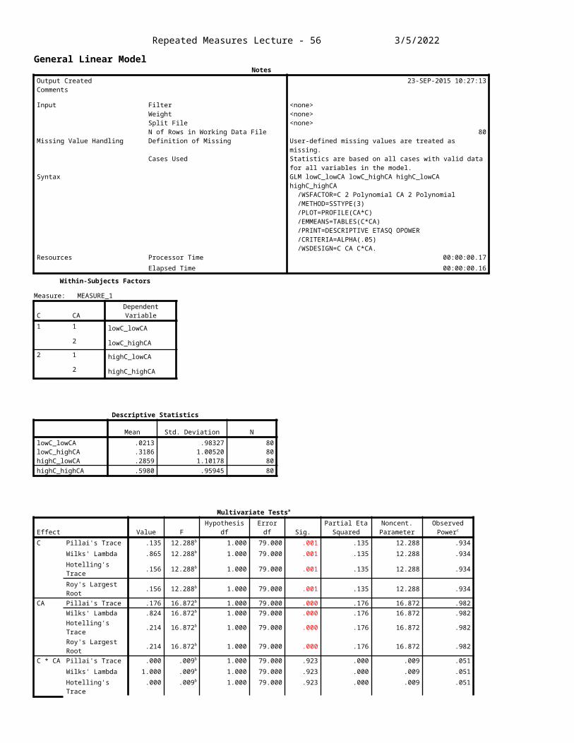
General Linear ModelNotes
Output Created 23-SEP-2015 10:27:13Comments
Input Filter <none>Weight <none>Split File <none>N of Rows in Working Data File 80
Missing Value Handling Definition of Missing User-defined missing values are treated as missing.Cases Used Statistics are based on all cases with valid data for all variables in
the model.Syntax GLM lowC_lowCA lowC_highCA highC_lowCA highC_highCA
/WSFACTOR=C 2 Polynomial CA 2 Polynomial /METHOD=SSTYPE(3) /PLOT=PROFILE(CA*C) /EMMEANS=TABLES(C*CA) /PRINT=DESCRIPTIVE ETASQ OPOWER /CRITERIA=ALPHA(.05) /WSDESIGN=C CA C*CA.
Resources Processor Time 00:00:00.17Elapsed Time 00:00:00.16
Within-Subjects Factors
Measure: MEASURE_1
C CA Dependent Variable1 1 lowC_lowCA
2 lowC_highCA2 1 highC_lowCA
2 highC_highCA
Descriptive Statistics
Mean Std. Deviation NlowC_lowCA .0213 .98327 80lowC_highCA .3186 1.00520 80highC_lowCA .2859 1.10178 80highC_highCA .5980 .95945 80
Multivariate Testsa
Effect Value F Hypothesis df Error df Sig.Partial Eta Squared
Noncent. Parameter
Observed Powerc
C Pillai's Trace .135 12.288b 1.000 79.000 .001 .135 12.288 .934Wilks' Lambda .865 12.288b 1.000 79.000 .001 .135 12.288 .934Hotelling's Trace .156 12.288b 1.000 79.000 .001 .135 12.288 .934Roy's Largest Root .156 12.288b 1.000 79.000 .001 .135 12.288 .934
CA Pillai's Trace .176 16.872b 1.000 79.000 .000 .176 16.872 .982Wilks' Lambda .824 16.872b 1.000 79.000 .000 .176 16.872 .982Hotelling's Trace .214 16.872b 1.000 79.000 .000 .176 16.872 .982Roy's Largest Root .214 16.872b 1.000 79.000 .000 .176 16.872 .982
C * CA Pillai's Trace .000 .009b 1.000 79.000 .923 .000 .009 .051Wilks' Lambda 1.000 .009b 1.000 79.000 .923 .000 .009 .051Hotelling's Trace .000 .009b 1.000 79.000 .923 .000 .009 .051Roy's Largest Root .000 .009b 1.000 79.000 .923 .000 .009 .051
a. Design: Intercept Within-subjects Design: C + CA + C * CAb. Exact statisticc. Computed using alpha = .05
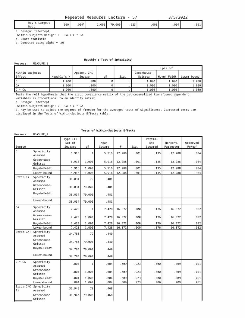
Mauchly's Test of Sphericitya
Measure: MEASURE_1
Within-subjects Effect Mauchly's WApprox. Chi-
Square df Sig.
Epsilonb
Greenhouse-Geisser Huynh-Feldt Lower-bound
C 1.000 .000 0 . 1.000 1.000 1.000CA 1.000 .000 0 . 1.000 1.000 1.000C * CA 1.000 .000 0 . 1.000 1.000 1.000Tests the null hypothesis that the error covariance matrix of the orthonormalized transformed dependent variables is proportional to an identity matrix.
Repeated Measures Lecture - 37 5/7/2023a. Design: Intercept Within-subjects Design: C + CA + C * CAb. May be used to adjust the degrees of freedom for the averaged tests of significance. Corrected tests are displayed in the Tests of Within-Subjects Effects table.
Tests of Within-Subjects EffectsMeasure: MEASURE_1
SourceType III Sum of Squares df
Mean Square F Sig.
Partial Eta Squared
Noncent. Parameter
Observed Powera
C Sphericity Assumed 5.916 1 5.916 12.288 .001 .135 12.288 .934Greenhouse-Geisser 5.916 1.000 5.916 12.288 .001 .135 12.288 .934
Huynh-Feldt 5.916 1.000 5.916 12.288 .001 .135 12.288 .934Lower-bound 5.916 1.000 5.916 12.288 .001 .135 12.288 .934
Error(C) Sphericity Assumed 38.034 79 .481
Greenhouse-Geisser 38.034 79.000 .481
Huynh-Feldt 38.034 79.000 .481
Lower-bound 38.034 79.000 .481
CA Sphericity Assumed 7.428 1 7.428 16.872 .000 .176 16.872 .982Greenhouse-Geisser 7.428 1.000 7.428 16.872 .000 .176 16.872 .982
Huynh-Feldt 7.428 1.000 7.428 16.872 .000 .176 16.872 .982Lower-bound 7.428 1.000 7.428 16.872 .000 .176 16.872 .982
Error(CA) Sphericity Assumed 34.780 79 .440
Greenhouse-Geisser 34.780 79.000 .440
Huynh-Feldt 34.780 79.000 .440
Lower-bound 34.780 79.000 .440
C * CA Sphericity Assumed .004 1 .004 .009 .923 .000 .009 .051Greenhouse-Geisser .004 1.000 .004 .009 .923 .000 .009 .051
Huynh-Feldt .004 1.000 .004 .009 .923 .000 .009 .051Lower-bound .004 1.000 .004 .009 .923 .000 .009 .051
Error(C*CA) Sphericity Assumed 36.940 79 .468
Greenhouse-Geisser 36.940 79.000 .468
Huynh-Feldt 36.940 79.000 .468
Lower-bound 36.940 79.000 .468
a. Computed using alpha = .05
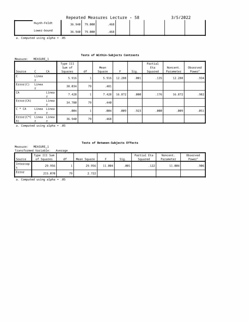
Tests of Within-Subjects ContrastsMeasure: MEASURE_1
Source C CAType III Sum of Squares df Mean Square F Sig.
Partial Eta Squared
Noncent. Parameter
Observed Powera
C Linear 5.916 1 5.916 12.288 .001 .135 12.288 .934
Error(C) Linear 38.034 79 .481
CA Linear 7.428 1 7.428 16.872 .000 .176 16.872 .982
Error(CA) Linear 34.780 79 .440
C * CA Linear Linear .004 1 .004 .009 .923 .000 .009 .051Error(C*CA) Linear Linear 36.940 79 .468
a. Computed using alpha = .05
Tests of Between-Subjects EffectsMeasure: MEASURE_1Transformed Variable: Average
SourceType III Sum of
Squares df Mean Square F Sig.Partial Eta Squared
Noncent. Parameter Observed Powera
Intercept 29.956 1 29.956 11.004 .001 .122 11.004 .906Error 215.070 79 2.722
a. Computed using alpha = .05
Repeated Measures Lecture - 38 5/7/2023
Repeated Measures Lecture - 39 5/7/2023
Estimated Marginal Means
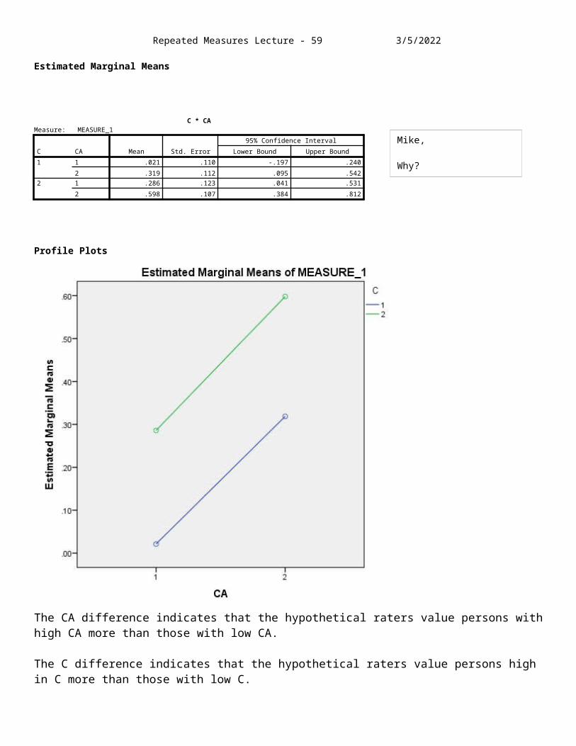
C * CAMeasure: MEASURE_1
C CA Mean Std. Error95% Confidence Interval
Lower Bound Upper Bound1 1 .021 .110 -.197 .240
2 .319 .112 .095 .5422 1 .286 .123 .041 .531
2 .598 .107 .384 .812
Profile Plots
The CA difference indicates that the hypothetical raters value persons with high CA more than those with low CA.
The C difference indicates that the hypothetical raters value persons high in C more than those with low C.
There is no interaction of the effectsof CA and C on ratings.
Mike,
Why?

Repeated Measures Lecture - 40 5/7/2023
Repeated Measures Skipped in 20161 Quantitative Between Subject Factor
1 Repeated Measures FactorNhung Nguyen’s dissertation data.
Nhung’s dissertation
1. Gave the Big 5 to 200 persons under two instruction conditions- once to respond honestly (Honest instruction) and again to respond in a “way that would best guarantee that you would get a customer service representative job.” (Instructed Faking).2. Gave the Wonderlic test – a test of cognitive ability that correlates very highly with standard IQ tests.3. Computed a faking ability score for each Big 5 dimension. This score was computed as the difference between the score under the Faking instruction and the score under the Honest instruction standardized so that faking ability scores on the Big Five dimensions were comparable. Called faking ability because participants were instructed to fake in the Instructed Faking condition.
Questions: 1. The Repeated Measures Main Effect:
Are there differences in the mean faking amounts of the different Big 5 Personality dimensions? That is, are the Big Five dimensions equally fakable?
2. The Between-subjects Main Effect:Are there differences in overall average faking between the various levels of cognitive ability? Did people who scored high on cognitive ability fake more than those who score low? Put another way: is there a relationship between faking ability and cognitive ability?
3. The Interaction of the Between-subjects and Repeated Measures Effects:Are differences in faking between the Big 5 measures the same across levels of cognitive ability?
orIs the relationship of faking ability to cognitive ability the same for different Big 5 dimensions.
The analysis is a repeated measures ANOVA with a Quantitative Between-subjects factor (the Wonderlic scores).
Because the Between-subjects Factor is quantitative, it will be specified differently than a nominal factor and the effects associated with it will be interpreted and presented differently than those in the previous example, which involved a nominal (group0vs1) between-subjects factor.
GET FILE='E:\MdbR\Nhung\SJTPaper\ThesisPaperFile030907.sav'.GLM dsurg dagree dcons des dopen WITH gscore /WSFACTOR = persdim 5 Polynomial /METHOD = SSTYPE(3) /PLOT = PROFILE( persdim ) /EMMEANS = TABLES(persdim) WITH(gscore=MEAN) /PRINT = DESCRIPTIVE ETASQ OPOWER /CRITERIA = ALPHA(.05) /WSDESIGN = persdim /DESIGN = gscore .
The syntax generated by the pull down menus shown below.
Repeated Measures Lecture - 41 5/7/2023Specification of Factors: Analyze -> General Linear Model -> Repeated Measures
Quantitative between-subjects factors must be put in the covariates box in GLM.
Repeated Measures Lecture - 42 5/7/2023
Hypotheses Tested
The Repeated Measures Main Effect (Surgency is extraversion)
µdsurg µdagree µdcons µdes µdopen

Repeated Measures Lecture - 43 5/7/2023
H0: Equality of means of population of faking scores on the 5 personality dimensions.
Repeated Measures Lecture - 44 5/7/2023The Between-subjects Main Effect
H0: The correlation of gscore with the average difference scores in population is 0.
Note that this hypothesis is NOT stated as equality of means. If we had observed, say, 50 people with CA = 20, 50 with CA=25, and 50 with CA=30, and 50 with CA=35, then it could have been stated as a hypothesis that the means of the faking scores at the 4 levels of CA were equal. But since we have multiple CA values with just a few scores at each, perhaps only 1, it is more efficient to examine the relationship of faking to CA, rather than to examine the differences in means.
The Interaction of Persdim and gscore
H0: The correlation of gscore with individual dimension faking scores will be the same for each individual dimension.
or
Differences between dimension faking score means will be the same for each level of gscore.
Average Diff scores
-.11 = Av Diff Score 20 = Av Diff Score 3
-.10 = Av Diff Score 1
1.14 = Av Diff Score 4
1.15 = Av Diff Score 5
0.86 = Av Diff Score 6
-0.04 = Av Diff Score 7
0.06 = Av Diff Score 8
And so on . .
gscore
Faking Ability
Repeated Measures Lecture - 45 5/7/2023General Linear Model
The failure to meet the sphericity criterion means that we cannot use the “Sphericity Assumed” F printed below.
The multivariate tests below indicate that there is NOT a main effect of Persdim (Personality dimension). This means that there are not overall significant differences in the amount of faking between the 5 dimensions.
The significant interaction suggests, however, that there are gscore-specific differences in the amount of faking between the 5 dimensions, i.e., differences that vary with gscore..
Equivalently, the interaction means that the correlation of gscore with faking of each dimensions varies from one dimension to the next.
Within-Subjects Factors
Measure: MEASURE_1
DSURG
DAGREE
DCONS
DES
DOPEN
PERSDIM1
2
3
4
5
DependentVariable
Descriptive Statistics
.4797 1.01526 203
.3556 1.00172 203
.5854 .97258 203
.7474 1.06989 203
.3921 .98581 203
DSURG
DAGREE
DCONS
DES
DOPEN
Mean Std. Dev iation N
Mu ltiv a ria te T e s ts c
.0 4 0 2 .0 4 1 b 4 .0 0 0 1 9 8 .0 0 0 .0 9 0 .0 4 0 8 .1 6 3 .6 0 3
.9 6 0 2 .0 4 1 b 4 .0 0 0 1 9 8 .0 0 0 .0 9 0 .0 4 0 8 .1 6 3 .6 0 3
.0 4 1 2 .0 4 1 b 4 .0 0 0 1 9 8 .0 0 0 .0 9 0 .0 4 0 8 .1 6 3 .6 0 3
.0 4 1 2 .0 4 1b
4 .0 0 0 1 9 8 .0 0 0 .0 9 0 .0 4 0 8 .1 6 3 .6 0 3
.0 5 1 2 .6 3 5 b 4 .0 0 0 1 9 8 .0 0 0 .0 3 5 .0 5 1 1 0 .5 3 8 .7 3 0
.9 4 9 2 .6 3 5 b 4 .0 0 0 1 9 8 .0 0 0 .0 3 5 .0 5 1 1 0 .5 3 8 .7 3 0
.0 5 3 2 .6 3 5 b 4 .0 0 0 1 9 8 .0 0 0 .0 3 5 .0 5 1 1 0 .5 3 8 .7 3 0
.0 5 3 2 .6 3 5b
4 .0 0 0 1 9 8 .0 0 0 .0 3 5 .0 5 1 1 0 .5 3 8 .7 3 0
P illa i's T ra c e
Wilk s ' L a mb d a
Ho te llin g 's T ra c e
Ro y 's L a rg e s tRo o t
P illa i's T ra c e
Wilk s ' L a mb d a
Ho te llin g 's T ra c e
Ro y 's L a rg e s tRo o t
E ffe c tP E RS D IM
P E RS D IM *GS COR E
V a lu e F Hy p o th e s is d f E rro r d f S ig .P a rtia l E ta
S q u a re dNo n c e n t.P a ra me te r Ob s e rv e d P o w e r
a
Co mp u te d u s in g a lp h a = .0 5a .
E x a c t s ta tis ticb .
De s ig n : In te rc e p t+ GS COR E With in S u b je c ts D e s ig n : P E R S D IM
c .
Ma uchly 's Tes t of Sphericity b
Me as ure : MEASURE_1
.88 8 23 .663 9 .00 5 .946 .97 1 .250
With in Sub jec tsEffe c tPERSDIM
Ma uc h ly 's WAp prox .
Ch i-Squa re df Sig .Gre enhous e-
Ge is s er Huy nh-Feld t Lower-bound
Eps ilona
Tes ts the nu ll hy po thes is that th e e rror c ov a rianc e ma trix o f the o rthono rma liz e d trans fo rmed dep endent v a riab les is p roportion alto an iden tity matrix .
Ma y be us e d to ad jus t the deg ree s o f freedom for the av e raged tes ts of s ign ific anc e . Co rrec ted tes ts a re d is p lay ed inthe Tes ts of With in -Sub jec ts Effec ts ta b le .
a.
De s ign : In terc ep t+GSCORE With in Sub jec ts Des ign: PERSDIM
b.

Repeated Measures Lecture - 46 5/7/2023
The Tests of Within-subjects Contrasts are automatically printed, but make no sense since the personality dimensions are not on a quantitative dimension.
The significant main effect of gscore means that there is a correlation of overall faking with cognitive ability. That is, there are differences in amount of faking at different levels of cognitive ability.
Inspection of the graph below shows that it’s positive – smarter people faked more.
T e s ts o f With in -S u b je c ts E ffe c ts
Me a s u re : ME A S UR E _ 1
5 .4 3 7 4 1 .3 5 9 2 .2 1 7 .0 6 6 .0 11 8 .8 6 6 .6 5 3
5 .4 3 7 3 .7 8 5 1 .4 3 7 2 .2 1 7 .0 6 9 .0 11 8 .3 8 9 .6 3 5
5 .4 3 7 3 .8 8 5 1 .3 9 9 2 .2 1 7 .0 6 8 .0 11 8 .6 1 3 .6 4 4
5 .4 3 7 1 .0 0 0 5 .4 3 7 2 .2 1 7 .1 3 8 .0 11 2 .2 1 7 .3 1 7
6 .0 6 7 4 1 .5 1 7 2 .4 7 4 .0 4 3 .0 1 2 9 .8 9 4 .7 0 8
6 .0 6 7 3 .7 8 5 1 .6 0 3 2 .4 7 4 .0 4 6 .0 1 2 9 .3 6 1 .6 9 0
6 .0 6 7 3 .8 8 5 1 .5 6 1 2 .4 7 4 .0 4 5 .0 1 2 9 .6 11 .6 9 8
6 .0 6 7 1 .0 0 0 6 .0 6 7 2 .4 7 4 .11 7 .0 1 2 2 .4 7 4 .3 4 7
4 9 2 .9 8 1 8 0 4 .6 1 3
4 9 2 .9 8 1 7 6 0 .7 0 0 .6 4 8
4 9 2 .9 8 1 7 8 0 .9 7 4 .6 3 1
4 9 2 .9 8 1 2 0 1 .0 0 0 2 .4 5 3
S p h e ric ity A s s u me d
Gre e n h o u s e -Ge is s er
Hu y n h -F e ld t
L o w e r-b o u n d
S p h e ric ity A s s u me d
Gre e n h o u s e -Ge is s er
Hu y n h -F e ld t
L o w e r-b o u n d
S p h e ric ity A s s u me d
Gre e n h o u s e -Ge is s er
Hu y n h -F e ld t
L o w e r-b o u n d
S o u rc eP E R S D IM
P E R S D IM *GS C OR E
E rro r(P E R S D IM)
T y p e III S u mo f S q u a re s d f Me a n S q u a re F S ig .
P a rtia l E taS q u a re d
No n c e n t.P a ra me te r Ob s e rv e d P o w e r
a
Co mp u te d u s in g a lp h a = .0 5a .
T e s ts o f With in -Su b je c ts Co n tra s ts
Me a s u re : ME AS URE _ 1
3 .7 1 5 1 3 .7 1 5 5 .4 5 2 .0 2 1 .0 2 6 5 .4 5 2 .6 4 2
.0 5 2 1 .0 5 2 .0 8 8 .7 6 8 .0 0 0 .0 8 8 .0 6 0
.0 5 8 1 .0 5 8 .0 7 9 .7 7 9 .0 0 0 .0 7 9 .0 5 9
1 .6 1 2 1 1 .6 1 2 3 .5 9 7 .0 5 9 .0 1 8 3 .5 9 7 .4 7 1
2 .9 9 6 1 2 .9 9 6 4 .3 9 7 .0 3 7 .0 2 1 4 .3 9 7 .5 5 1
.6 2 2 1 .6 2 2 1 .0 4 8 .3 0 7 .0 0 5 1 .0 4 8 .1 7 5
.6 8 1 1 .6 8 1 .9 3 4 .3 3 5 .0 0 5 .9 3 4 .1 6 1
1 .7 6 7 1 1 .7 6 7 3 .9 4 3 .0 4 8 .0 1 9 3 .9 4 3 .5 0 7
1 3 6 .9 6 9 2 0 1 .6 8 1
11 9 .3 1 2 2 0 1 .5 9 4
1 4 6 .6 2 1 2 0 1 .7 2 9
9 0 .0 7 9 2 0 1 .4 4 8
PE RS DIML in e a r
Qu a d ra tic
Cu b ic
Ord e r 4
L in e a r
Qu a d ra tic
Cu b ic
Ord e r 4
L in e a r
Qu a d ra tic
Cu b ic
Ord e r 4
So u rc ePE RS DIM
PE RS DIM *GS CORE
Erro r(P E RS DIM)
T y p e III S u mo f S q u a re s d f Me a n S q u a re F S ig .
Pa rtia l E taSq u a re d
No n c e n t.Pa ra me te r Ob s e rv e d P o we r
a
Co mp u te d u s in g a lp h a = .0 5a .
Te s ts of Be twee n-Subje c ts Effe c ts
Me a s u re : MEASURE_1
Tra n s fo rme d Va ria b le : Av e ra ge
6 .2 9 2 1 6 .2 9 2 2 .6 3 2 .10 6 .01 3 2 .6 3 2 .36 5
49 .9 2 4 1 49 .9 2 4 20 .8 8 2 .00 0 .09 4 20 .8 8 2 .99 5
48 0 .5 40 20 1 2 .3 9 1
So u rc eIn te rc e p t
GSCORE
Erro r
Ty p e III Su mo f Sq u a re s d f Me a n Sq u a re F Sig .
Pa rtia l EtaSq u a red
No n c en t.Pa ra me te r Ob s e rv e d Powe ra
Co mp u te d u s in g a lpha = .0 5a .

Repeated Measures Lecture - 47 5/7/2023Estimated Marginal Means
Profile Plots
Graphing the Main Effect of gscore.I computed an average faking score (those values illustrated on the right on p. 22 above.)graph /scatterplot = gscore with fakescor.
Graph
This is a display of the main effect of cognitive ability. The average difference scores are called FAKESCOR in this plot. On the right, persons with similar gscore values have been grouped together. This shows the positive relationship of faking to Gscore more strikingly.
Ext Agr Con Sta Opn
These are identical to the observed means since there is only one group of respondents.Dimensions are listed as E A C S O.So the largest amount of faking was in the Emotional Stability dimension (4th in the list). The least was in Agreeableness and Openness. But remember that the differences in means were not officially significant.
Note – Persdim main effect was not significant, so this graph shouldn’t be overinterpreted.
PERSDIM
Me a s u re : MEASURE_ 1
.4 8 0 a .0 6 9 .3 4 4 .6 1 5
.3 5 6 a .0 6 8 .2 2 2 .4 8 9
.5 8 5 a .0 6 7 .4 5 3 .7 1 8
.7 4 7 a .0 7 3 .6 0 4 .8 9 1
.3 9 2 a .0 6 9 .2 5 6 .5 2 8
PERSDIM1
2
3
4
5
Me a n Std . Erro r L o we r Bo u n dUp p e r Bo u n d
9 5 % Co n f i d e n c e In te rv a l
Co v a ri a te s a p p e a ri n g i n th e mo d e l a re e v a l u a te d a t th efo l l o wi n g v a l u e s : GSCORE wo n d e rl i c te s t s c o re = 2 4 .6 1 .
a .
Estimated Marginal Means of MEASURE_1
PERSDIM
54321
Es
tim
ate
d M
arg
ina
l M
ea
ns
. 8
. 7
. 6
. 5
. 4
. 3
wo n d e rl i c te s t s c o re
50403020100
FA
KE
SC
OR
4
3
2
1
0
-1
-2 Rsq = 0. 0941

Repeated Measures Lecture - 48 5/7/2023The interactions.
Recall what the interaction is: The relationship of average faking to gscore differed across dimensions.
Below are displays of the relationship of faking for each dimension to cognitive ability. These displays are analogous to the “interaction” plots when the between-subjects factor is a categorical factor.
I’m not sure of the explanation of the interaction. Why is the relationship of faking to cognitive ability stronger for Extraversion than it is for Openness, for example? That is, smart people faked Extraversion a lot more than less smart people did. But smart people didn’t fake Openness much more than less smart people. ??
graph /scatterplot = gscore with dsurg.
Graph r = +.27
graph /scatterplot = gscore with dagree.
Graph r = +.28
graph /scatterplot = gscore with dcons.
Graph r = +.19
graph /scatterplot = gscore with des.
Graph r = +.26
graph /scatterplot = gscore with dopen.
Graph r = +.09
It may be that for some items, there may be disagreement on what constitutes a “good” response. That is, some people might have thought that agreeing was the appropriate way to fake while others thought that disagreeing was the appropriate way to fake. The result was that the relationships of faking to cognitive ability was suppressed for those items.
wo n d e rl i c te s t s c o re
50403020100
DS
UR
G
5
4
3
2
1
0
-1
-2 Rsq = 0. 0744
wo n d e rl i c te s t s c o re
50403020100
DA
GR
EE
4
3
2
1
0
-1
-2
-3
-4 Rsq = 0. 0802
wo n d e rl i c te s t s c o re
50403020100
DC
ON
S
6
4
2
0
-2
-4 Rsq = 0. 0362
wo n d e rl i c te s t s c o re
50403020100D
ES
5
4
3
2
1
0
-1
-2 Rsq = 0. 0685
wo n d e rl i c te s t s c o re
50403020100
DO
PE
N
4
3
2
1
0
-1
-2
-3 Rsq = 0. 0076
Repeated Measures Lecture - 49 5/7/2023
Using a correlation matrix to examine the individual dimension correlations.
correlation gscore dsurg to dopen fakescore.
Correlations
Repeated Measures Lecture - 49 05/07/23
W ar ni ngs
Text : FAKESCO REA var iable nam e is m or e t han 8 char act er s long. O nly t he f ir st 8 char act er s will be used.
Co rre la tio n s
1 .2 7 3 .2 8 3 .1 9 0 .2 6 2 .0 8 7 .3 0 7
. .0 0 0 .0 0 0 .0 0 7 .0 0 0 .2 1 5 .0 0 0
2 0 3 2 0 3 2 0 3 2 0 3 2 0 3 2 0 3 2 0 3
.2 7 3 1 .4 1 6 .3 2 9 .4 5 2 .3 7 5 .7 1 9
.0 0 0 . .0 0 0 .0 0 0 .0 0 0 .0 0 0 .0 0 0
2 0 3 2 0 3 2 0 3 2 0 3 2 0 3 2 0 3 2 0 3
.2 8 3 .4 1 6 1 .3 9 7 .2 6 0 .3 3 1 .6 6 6
.0 0 0 .0 0 0 . .0 0 0 .0 0 0 .0 0 0 .0 0 0
2 0 3 2 0 3 2 0 3 2 0 3 2 0 3 2 0 3 2 0 3
.1 9 0 .3 2 9 .3 9 7 1 .4 9 8 .4 3 5 .7 3 6
.0 0 7 .0 0 0 .0 0 0 . .0 0 0 .0 0 0 .0 0 0
2 0 3 2 0 3 2 0 3 2 0 3 2 0 3 2 0 3 2 0 3
.2 6 2 .4 5 2 .2 6 0 .4 9 8 1 .4 5 1 .7 5 0
.0 0 0 .0 0 0 .0 0 0 .0 0 0 . .0 0 0 .0 0 0
2 0 3 2 0 3 2 0 3 2 0 3 2 0 3 2 0 3 2 0 3
.0 8 7 .3 7 5 .3 3 1 .4 3 5 .4 5 1 1 .7 1 8
.2 1 5 .0 0 0 .0 0 0 .0 0 0 .0 0 0 . .0 0 0
2 0 3 2 0 3 2 0 3 2 0 3 2 0 3 2 0 3 2 0 3
.3 0 7 .7 1 9 .6 6 6 .7 3 6 .7 5 0 .7 1 8 1
.0 0 0 .0 0 0 .0 0 0 .0 0 0 .0 0 0 .0 0 0 .
2 0 3 2 0 3 2 0 3 2 0 3 2 0 3 2 0 3 2 0 3
Pe a rs o nCo rre la tio n
S ig . (2 -ta ile d )
N
Pe a rs o nCo rre la tio n
S ig . (2 -ta ile d )
N
Pe a rs o nCo rre la tio n
S ig . (2 -ta ile d )
N
Pe a rs o nCo rre la tio n
S ig . (2 -ta ile d )
N
Pe a rs o nCo rre la tio n
S ig . (2 -ta ile d )
N
Pe a rs o nCo rre la tio n
S ig . (2 -ta ile d )
N
Pe a rs o nCo rre la tio n
S ig . (2 -ta ile d )
N
GS CORE wo n d e rlic te s ts c o re
DS URG
DA GRE E
DCONS
DE S
DOP E N
F A K E S COR
GS CORE wo n d e rlic te s t
s c o re DS URG DA GRE E DCONS DE S DOP E N F A K E S COR
Repeated Measures Lecture - 50 5/7/2023
Repeated Measures ANOVA – Skipped in 20151 Between Groups Factor
2 Repeated Measures Factors in factorial arrangementThe data are from Myers & Well, p 313 although the story describing the data is different from theirs. Memory for two types of event, one of some interest to the persons (C1), the other of less interest to them (C2) is tested at three time periods (B1, B2, and B3). The tests are performed under two conditions of distraction, much distraction (A1) and little distraction (A2). The interest here is on the effects of interest on memory, the effects of distraction on memory, and the the interaction of interest and distraction – whether the effect of distraction is the same for memory of interesting and uninteresting material. The data matrix looks as follows . .
C1B1 C1B2 C1B3 C2B1 C2B2 C2B3 A
80 48 45 76 45 41 1 46 37 34 42 34 33 1 51 49 36 45 38 30 1 72 57 50 66 51 42 1 68 40 33 58 38 30 1 65 44 36 56 37 28 1
70 55 52 68 57 56 2 88 69 66 91 74 70 2 58 60 54 50 41 38 2 63 57 52 61 58 56 2 78 81 75 79 78 74 2 84 82 80 80 73 76 2
Specify the factor that varies slowest across columns first
Then specif the factor whose levels vary fastest next, in this case the B factor . . .
Repeated Measures Lecture - 50 05/07/23
Interestingmaterial
Uninterestingmaterial
Much distraction
Littledistraction
Mike – show the pull down menus in more detail.

Repeated Measures Lecture - 51 5/7/2023
Click on the “Define” button, then . . .
Repeated Measures Lecture - 51 05/07/23

Repeated Measures Lecture - 52 5/7/2023
Click on the name of each variable in the left-hand field and click on the right-pointing arrow to move the name into the “Withing-Subjects Variables” field.
GLM c1b1 c1b2 c1b3 c2b1 c2b2 c2b3 BY a /WSFACTOR = c 2 Polynomial b 3 Polynomial /METHOD = SSTYPE(3) /PLOT = PROFILE( b*a*c ) /PRINT = DESCRIPTIVE ETASQ OPOWER HOMOGENEITY /CRITERIA = ALPHA(.05) /WSDESIGN = c b c*b /DESIGN = a .
I believe it’s given because the number of persons in each cell is not larger than the number of measures on each person.
Repeated Measures Lecture - 52 05/07/23
Warnings
Box's Test of Equality of CovarianceMatrices is not computed becausethere are fewer than twononsingular cell covariancematrices.
Much distraction
Littledistraction
Much distraction
Littledistraction
Much distraction
Littledistraction
µB1 µB2 µB3
Repeated Measures Lecture - 53 5/7/2023
Hypotheses tested
The C (Interest) - Repeated Measures Main Effect
C1B1 C1B2 C1B3 C2B1 C2B2 C2B3 A
80 48 45 76 45 41 1 46 37 34 42 34 33 1 51 49 36 45 38 30 1 72 57 50 66 51 42 1 68 40 33 58 38 30 1 65 44 36 56 37 28 1 70 55 52 68 57 56 2 88 69 66 91 74 70 2 58 60 54 50 41 38 2 63 57 52 61 58 56 2 78 81 75 79 78 74 2 84 82 80 80 73 76 2
The B (Time) - Repeated Measures Main Effect
C1B1 C1B2 C1B3 C2B1 C2B2 C2B3 A
80 48 45 76 45 41 1 46 37 34 42 34 33 1 51 49 36 45 38 30 1 72 57 50 66 51 42 1 68 40 33 58 38 30 1 65 44 36 56 37 28 1 70 55 52 68 57 56 2 88 69 66 91 74 70 2 58 60 54 50 41 38 2 63 57 52 61 58 56 2 78 81 75 79 78 74 2 84 82 80 80 73 76 2
The A – Distraction - Between-Subjects Main Effect
C1B1 C1B2 C1B3 C2B1 C2B2 C2B3 A
80 48 45 76 45 41 46 37 34 42 34 33 51 49 36 45 38 30 72 57 50 66 51 42 68 40 33 58 38 30 65 44 36 56 37 28
70 55 52 68 57 56 88 69 66 91 74 70 58 60 54 50 41 38 63 57 52 61 58 56 78 81 75 79 78 74 84 82 80 80 73 76
Repeated Measures Lecture - 53 05/07/23
µC1 µC2
µA1
µA2
Sample is treated as one giant group for the repeated measures comparisons
Sample is treated as one giant group for the repeated measures comparisons

Repeated Measures Lecture - 54 5/7/2023
General Linear Model
Repeated Measures Lecture - 54 05/07/23
Within-Subjects Factors
Measure: MEASURE_1
C1B1
C1B2
C1B3
C2B1
C2B2
C2B3
B1
2
3
1
2
3
C1
2
DependentVariable
Between-Subjects Factors
6
6
1
2
AValue Label N
Descriptive Statistics
63.67 12.88 6
73.50 11.86 6
68.58 12.87 12
45.83 7.14 6
67.33 11.98 6
56.58 14.64 12
39.00 6.87 6
63.17 12.37 6
51.08 15.82 12
57.17 12.75 6
71.50 14.79 6
64.33 15.14 12
40.50 6.28 6
63.50 14.07 6
52.00 15.88 12
34.00 6.03 6
61.67 14.50 6
47.83 17.91 12
A1
2
Total
1
2
Total
1
2
Total
1
2
Total
1
2
Total
1
2
Total
C1B1
C1B2
C1B3
C2B1
C2B2
C2B3
Mean Std. Dev iation N
Repeated Measures Lecture - 55 5/7/2023
The multivariate tests. The less powerful but more robust multivariate tests are always printed first. These tests indicate that there is a significant effect associated with Factor C (Interest), with Factor B (Time), and with the B * A (Time by Distraction) interaction.
The significant C Main effect indicates that the mean amount recalled depends on the Interest.
The significant B main effect indicates that the mean amount recalled depends on the time at which recall occurred.
The significant B*A interaction indicates that the change in mean amount over time is different for persons under much distraction than it is for persons under little distraction.
Repeated Measures Lecture - 55 05/07/23
M ul t i var i at e Test sc
. 442 7. 935b 1. 000 10. 000 . 018 . 442 7. 935 . 719
. 558 7. 935b 1. 000 10. 000 . 018 . 442 7. 935 . 719
. 793 7. 935b 1. 000 10. 000 . 018 . 442 7. 935 . 719
. 793 7. 935b 1. 000 10. 000 . 018 . 442 7. 935 . 719
. 109 1. 226b 1. 000 10. 000 . 294 . 109 1. 226 . 171
. 891 1. 226b 1. 000 10. 000 . 294 . 109 1. 226 . 171
. 123 1. 226b 1. 000 10. 000 . 294 . 109 1. 226 . 171
. 123 1. 226b 1. 000 10. 000 . 294 . 109 1. 226 . 171
. 893 37. 678 b 2. 000 9. 000 . 000 . 893 75. 356 1. 000
. 107 37. 678 b 2. 000 9. 000 . 000 . 893 75. 356 1. 000
8. 373 37. 678 b 2. 000 9. 000 . 000 . 893 75. 356 1. 000
8. 373 37. 678 b 2. 000 9. 000 . 000 . 893 75. 356 1. 000
. 567 5. 883b 2. 000 9. 000 . 023 . 567 11. 766 . 734
. 433 5. 883b 2. 000 9. 000 . 023 . 567 11. 766 . 734
1. 307 5. 883b 2. 000 9. 000 . 023 . 567 11. 766 . 734
1. 307 5. 883b 2. 000 9. 000 . 023 . 567 11. 766 . 734
. 323 2. 150b 2. 000 9. 000 . 173 . 323 4. 299 . 329
. 677 2. 150b 2. 000 9. 000 . 173 . 323 4. 299 . 329
. 478 2. 150b 2. 000 9. 000 . 173 . 323 4. 299 . 329
. 478 2. 150b 2. 000 9. 000 . 173 . 323 4. 299 . 329
. 186 1. 028b 2. 000 9. 000 . 396 . 186 2. 055 . 177
. 814 1. 028b 2. 000 9. 000 . 396 . 186 2. 055 . 177
. 228 1. 028b 2. 000 9. 000 . 396 . 186 2. 055 . 177
. 228 1. 028b 2. 000 9. 000 . 396 . 186 2. 055 . 177
Pilla i's Tr ac e
W ilk s ' Lam bda
Hot e lling 's Tr ac e
Roy 's Lar ges t Root
Pilla i's Tr ac e
W ilk s ' Lam bda
Hot e lling 's Tr ac e
Roy 's Lar ges t Root
Pilla i's Tr ac e
W ilk s ' Lam bda
Hot e lling 's Tr ac e
Roy 's Lar ges t Root
Pilla i's Tr ac e
W ilk s ' Lam bda
Hot e lling 's Tr ac e
Roy 's Lar ges t Root
Pilla i's Tr ac e
W ilk s ' Lam bda
Hot e lling 's Tr ac e
Roy 's Lar ges t Root
Pilla i's Tr ac e
W ilk s ' Lam bda
Hot e lling 's Tr ac e
Roy 's Lar ges t Root
Ef f ec tC
C * A
B
B * A
C * B
C * B * A
Value F Hy pot hes is dfEr r or df Sig. Et a Squar edNonc ent .
Par am et erO bs er v ed
Powera
Com put ed us ing alpha = . 05a.
Ex ac t s t at is t icb.
Des ign: I nt er c ept +A W it h in Subjec t s Des ign: C+B+C* B
c .
Repeated Measures Lecture - 56 5/7/2023
The sphericity test . Mauchly's test indicates that the sphericity condition is NOT met. So we must either go with the multivariate tests or use one of the tests which adjusts for lack of sphericity. Fortunately, they all give the same result with respect to significance and they all agree with the multivariate tests with respect to significance, so the point is moot.
Repeated Measures Lecture - 56 05/07/23
M auchl y's Test of Spher i ci t yb
M easur e: M EASURE_1
1. 000 . 000 0 . 1. 000 1. 000 1. 000
. 263 12. 031 2 . 002 . 576 . 668 . 500
. 491 6. 402 2 . 041 . 663 . 801 . 500
W it hin Subject s Ef f ectC
B
C * B
M auchly's WAppr ox.
Chi- Squar e df Sig.G r eenhouse- G eisser Huynh- Feldt Lower - bound
Epsilona
Test s t he null hypot hesis t hat t he er r or covar iance m at r ix of t he or t honor m alized t r ansf or m ed dependentvar iables is pr opor t ional t o an ident it y m at r ix.
M ay be used t o adjust t he degr ees of f r eedom f or t he aver aged t est s of signif icance. Cor r ect edt est s ar e displayed in t he Test s of W it hin- Subject s Ef f ect s t able.
a.
Design: I nt er cept +A W it hin Subject s Design: C+B+C* B
b.
Repeated Measures Lecture - 57 5/7/2023
Repeated Measures Lecture - 57 05/07/23
Te sts of Within-Subje cts Effec ts
Me as ure : MEASURE_1
29 2 .0 14 1 29 2 .0 14 7.9 35 .01 8 .44 2 7.9 35 .71 9
29 2 .0 14 1.0 00 29 2 .0 14 7.9 35 .01 8 .44 2 7.9 35 .71 9
29 2 .0 14 1.0 00 29 2 .0 14 7.9 35 .01 8 .44 2 7.9 35 .71 9
29 2 .0 14 1.0 00 29 2 .0 14 7.9 35 .01 8 .44 2 7.9 35 .71 9
45 .12 5 1 45 .12 5 1.2 26 .29 4 .10 9 1.2 26 .17 1
45 .12 5 1.0 00 45 .12 5 1.2 26 .29 4 .10 9 1.2 26 .17 1
45 .12 5 1.0 00 45 .12 5 1.2 26 .29 4 .10 9 1.2 26 .17 1
45 .12 5 1.0 00 45 .12 5 1.2 26 .29 4 .10 9 1.2 26 .17 1
36 8 .0 28 10 36 .80 3
36 8 .0 28 10 .00 0 36 .80 3
36 8 .0 28 10 .00 0 36 .80 3
36 8 .0 28 10 .00 0 36 .80 3
36 83 .111 2 18 41 .55 6 36 .41 0 .00 0 .78 5 72 .82 1 1.0 00
36 83 .111 1.1 51 31 99 .37 8 36 .41 0 .00 0 .78 5 41 .91 5 1.0 00
36 83 .111 1.3 35 27 58 .60 5 36 .41 0 .00 0 .78 5 48 .61 3 1.0 00
36 83 .111 1.0 00 36 83 .111 36 .41 0 .00 0 .78 5 36 .41 0 1.0 00
61 6 .3 33 2 30 8 .1 67 6.0 93 .00 9 .37 9 12 .18 6 .83 3
61 6 .3 33 1.1 51 53 5 .3 85 6.0 93 .02 7 .37 9 7.0 14 .65 2
61 6 .3 33 1.3 35 46 1 .6 26 6.0 93 .02 1 .37 9 8.1 35 .70 1
61 6 .3 33 1.0 00 61 6 .3 33 6.0 93 .03 3 .37 9 6.0 93 .60 6
10 11 .5 56 20 50 .57 8
10 11 .5 56 11.5 12 87 .87 0
10 11 .5 56 13 .35 1 75 .76 4
10 11 .5 56 10 .00 0 10 1 .1 56
5.7 78 2 2.8 89 .69 1 .51 2 .06 5 1.3 83 .15 0
5.7 78 1.3 25 4.3 59 .69 1 .46 0 .06 5 .91 6 .12 9
5.7 78 1.6 03 3.6 05 .69 1 .48 4 .06 5 1.1 08 .13 8
5.7 78 1.0 00 5.7 78 .69 1 .42 5 .06 5 .69 1 .117
7.0 00 2 3.5 00 .83 8 .44 7 .07 7 1.6 76 .17 3
7.0 00 1.3 25 5.2 82 .83 8 .40 9 .07 7 1.11 0 .14 6
7.0 00 1.6 03 4.3 67 .83 8 .42 7 .07 7 1.3 43 .15 8
7.0 00 1.0 00 7.0 00 .83 8 .38 2 .07 7 .83 8 .13 2
83 .55 6 20 4.1 78
83 .55 6 13 .25 3 6.3 04
83 .55 6 16 .02 9 5.2 13
83 .55 6 10 .00 0 8.3 56
Sp he ric ity As s u me d
Gre en ho us e-Ge is s er
Hu y n h-Fe ld t
Lo we r-bo un d
Sp he ric ity As s u me d
Gre en ho us e-Ge is s er
Hu y n h-Fe ld t
Lo we r-bo un d
Sp he ric ity As s u me d
Gre en ho us e-Ge is s er
Hu y n h-Fe ld t
Lo we r-bo un d
Sp he ric ity As s u me d
Gre en ho us e-Ge is s er
Hu y n h-Fe ld t
Lo we r-bo un d
Sp he ric ity As s u me d
Gre en ho us e-Ge is s er
Hu y n h-Fe ld t
Lo we r-bo un d
Sp he ric ity As s u me d
Gre en ho us e-Ge is s er
Hu y n h-Fe ld t
Lo we r-bo un d
Sp he ric ity As s u me d
Gre en ho us e-Ge is s er
Hu y n h-Fe ld t
Lo we r-bo un d
Sp he ric ity As s u me d
Gre en ho us e-Ge is s er
Hu y n h-Fe ld t
Lo we r-bo un d
Sp he ric ity As s u me d
Gre en ho us e-Ge is s er
Hu y n h-Fe ld t
Lo we r-bo un d
So urc eC
C * A
Erro r(C)
B
B * A
Erro r(B)
C * B
C * B * A
Erro r(C*B)
Ty pe III Su mof Squ are s df Me an Sq ua re F Sig . Eta Sq ua red
No nc en t.Pa ramete r
Ob s e rv e dPo we r
a
Co mp ute d u s in g a lpha = .0 5a.
Repeated Measures Lecture - 58 5/7/2023
Test of equality of variances across groups . Levene's test is for the between-subjects effects. It indicates generally that the variances are not significantly different.
Test of between-subjects main effect . The comparison between the two distracter conditions indicates that there is a significant difference in mean recall between the two.
Repeated Measures Lecture - 58 05/07/23
Levene's Test of E quality of E r r or Var iances a
.007 1 10 .936
3.186 1 10 .105
4.778 1 10 .054
.311 1 10 .589
5.205 1 10 .046
5.000 1 10 .049
C1B 1
C1B 2
C1B 3
C2B 1
C2B 2
C2B 3
F df1 df2 S ig.
Tests the null hypothesis that the error variance ofthe dependent variable is equal across groups.
Design: Intercept+A W ithin S ubjects Design: C+B +C* B
a.
Test s of Bet w een- Subj ect s Ef f ect s
M easur e: M EASURE_1
Tr ansf or m ed Var iable: Aver age
231767. 014 1 231767. 014 363. 878 . 000 . 973 363. 878 1. 000
7260. 125 1 7260. 125 11. 399 . 007 . 533 11. 399 . 860
6369. 361 10 636. 936
Sour ceI nt er cept
A
Er r or
Type I I I Sumof Squar es df M ean Squar e F Sig. Et a Squar ed
Noncent .Par am et er
O bser vedPower
a
Com put ed using alpha = . 05a.
Repeated Measures Lecture - 59 5/7/2023
Profile Plots
Repeated Measures Lecture - 59 05/07/23
Distraction.
Main Effect of A: Mean recall was better in the low distraction condition.
Time.
Main Effect of B: Mean recall decreased over time periods.
Estimated Marginal Means of MEASURE_1
A
Low dist r act ion condHigh dist r act ion con
Es
tim
ate
d M
arg
ina
l M
ea
ns
70
60
50
40
Estimated Marginal Means of MEASURE_1
B
321
Es
tim
ate
d M
arg
ina
l M
ea
ns
70
60
50
40

Repeated Measures Lecture - 60 5/7/2023
Repeated Measures Lecture - 60 05/07/23
Distraction by Time.
Interaction of A and B: The effect of distraction was greater at longer recall times. (This was the only significant interaction.)
Main Effect of Factor C: Mean recall was greater for more interesting material.
MoreInteresting
LessInteresting
Estimated Marginal Means of MEASURE_1
C
21
Es
tim
ate
d M
arg
ina
l M
ea
ns
59
58
57
56
55
54
Estimated Marginal Means of MEASURE_1
B
321
Es
tim
ate
d M
arg
ina
l M
ea
ns
80
70
60
50
40
30
A
High dist ract ion con
dit ion
Low dist ract ion cond
it ion
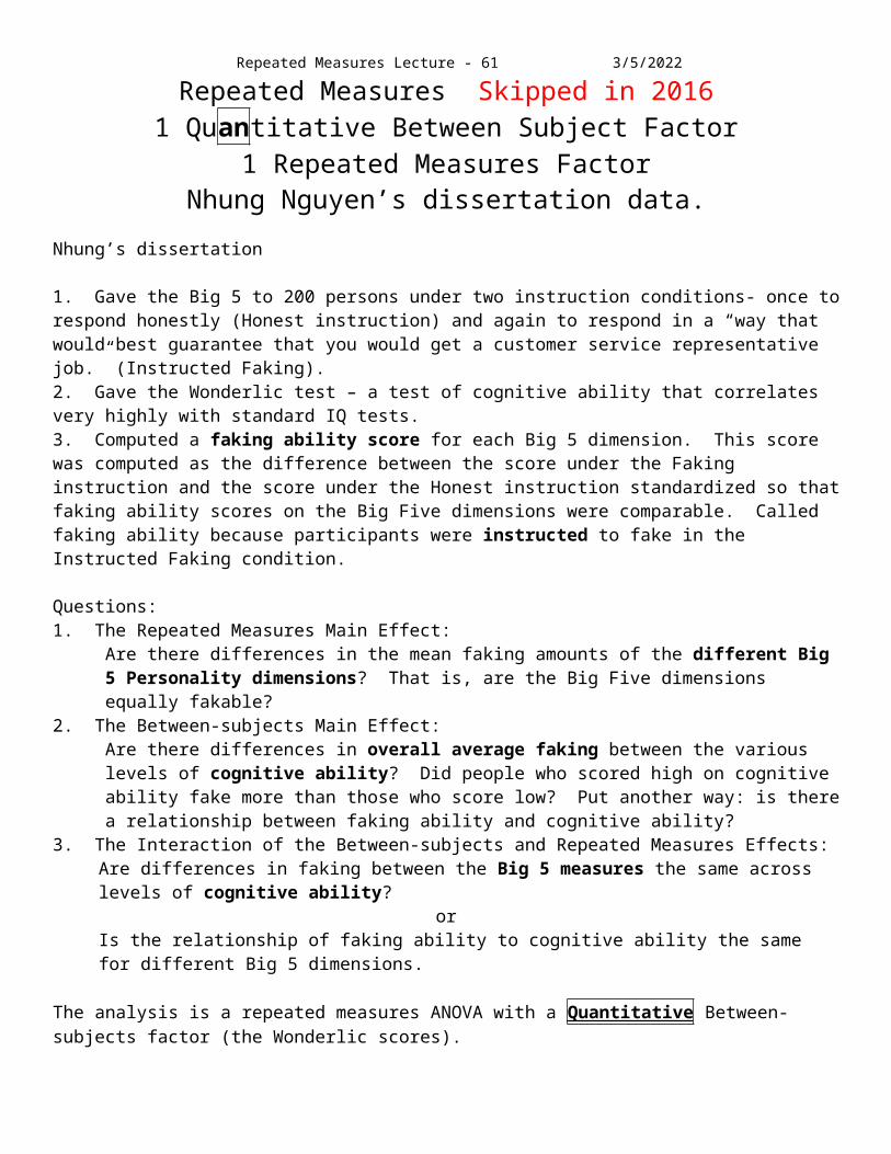
Repeated Measures Lecture - 61 5/7/2023
B * A * C
Repeated Measures Lecture - 61 05/07/23
Even though the three way interaction, B*A*C was not significant, it is of value to see how it would be visualized. A significant three way interaction means that a two-way interaction was not the same across levels of a third variable.
In this case, if the B*A*C interaction were significant, that would mean that the B*A interaction varied across levels of C. The way to visualize that is to plot the B*A interaction for each level of C. Those plots are on the left. The fact that they're nearly identical supports the fact that there was NO B*A*C interaction. If there had been, the two plots (one for C=1 and the other for C=2) would have been different.
So . . .
A two-way interaction is a difference of effect of one variable across levels of a second variable.
A three-way interaction is a difference of INTERACTION of two variables across levels of a third variable.
Estimated Marginal Means of MEASURE_1
At C = 1
B
321
Es
tim
ate
d M
arg
ina
l M
ea
ns
80
70
60
50
40
30
A
High dist ract ion con
dit ion
Low dist ract ion cond
it ion
Estimated Marginal Means of MEASURE_1
At C = 2
B
321
Es
tim
ate
d M
arg
ina
l M
ea
ns
80
70
60
50
40
30
A
High dist ract ion con
dit ion
Low dist ract ion cond
it ion