Embed Size (px)
Citation preview
NCAT Report 09-07 REPEATABILITY OF ASPHALT STRAIN GAUGES
By J. Richard Willis David Timm
October 2009
REPEATABILITY OF ASPHALT STRAIN GAUGES
By
J. Richard Willis, Ph.D. Assistant Research Professor
National Center for Asphalt Technology Auburn University, Auburn, Alabama
David H. Timm, Ph.D., P.E. Gottlieb Associate Professor
Department of Civil Engineering Auburn University, Auburn, Alabama
NCAT Report 09-07
October 2009

DISCLAIMER
The contents of this report reflect the views of the authors who are responsible for the facts and accuracy of the data presented herein. The contents do not necessarily reflect the official views or policies of the Alabama Department of Transportation, Florida Department of Transportation, Oklahoma Department of Transportation, Missouri Department of Transportation, Federal Highway Administration, or the National Center for Asphalt Technology, or Auburn University. This report does not constitute a standard, specification, or regulation.

Willis & Timm
ii
ACKNOWLEDGEMENT OF SPONSORSHIP The authors would like to thank the following organizations for their cooperation in funding and supporting the research documented in this report: Alabama Department of Transportation, Florida Department of Transportation, Oklahoma Department of Transportation, Missouri Department of Transportation, and the Federal Highway Administration.
Willis & Timm
iii
TABLE OF CONTENTS CHAPTER 1 – INTRODUCTION ................................................................................................. 1
Sources of Instrumentation Variability ....................................................................................... 1 Quantifying Variability ............................................................................................................... 3 2006 NCAT Pavement Test Track .............................................................................................. 4 Objectives ................................................................................................................................... 4 Scope ........................................................................................................................................... 4
CHAPTER 2 – TEST FACILITY AND INSTRUMENTATION .................................................. 5 Test Sections ............................................................................................................................... 5 Instrumentation ........................................................................................................................... 5 Installation................................................................................................................................... 7
CHAPTER 3 – BETWEEN GAUGE PRECISION UNDER LIVE TRAFFIC ............................. 8 Data Acquisition and Processing ................................................................................................ 8 Data Set Preparation ................................................................................................................... 9 Data Analysis .............................................................................................................................. 9
Gauge Orientation Comparisons .......................................................................................... 10 Axle Type Comparisons ........................................................................................................ 12 Section Specific Comparisons ............................................................................................... 13
Summary ................................................................................................................................... 15 CHAPTER 4 – WITHIN GAUGE REPEATABILITY UNDER FALLING WEIGHT DEFLECTOMETER LOADING ................................................................................................. 17
Methodology ............................................................................................................................. 17 Data Analysis ............................................................................................................................ 18
Gauge Orientation Comparisons .......................................................................................... 18 Load Level Comparisons ...................................................................................................... 19 Strain Magnitude Comparisons ............................................................................................ 22 Gauge Depth ......................................................................................................................... 24 Pavement Condition .............................................................................................................. 25
Summary ................................................................................................................................... 27 CHAPTER 5 – CONCLUSIONS AND RECOMMENDATIONS .............................................. 28
Conclusions ............................................................................................................................... 28 Recommendations ..................................................................................................................... 28
Willis & Timm
iv
List of Figures FIGURE 1 CTL ASG-152 strain gauge. ......................................................................................... 2 FIGURE 2 Cross-sections of 2006 structural sections. .................................................................. 5 FIGURE 3 Typical gauge array. ..................................................................................................... 6 FIGURE 4 Typical strain response. ................................................................................................ 9 FIGURE 5 Cumulative distribution for transverse and longitudinal gauges. ............................... 11 FIGURE 6 Effect of wheel wander on longitudinal and transverse gauges. ................................ 11 FIGURE 7 Axle type comparisons. .............................................................................................. 12 FIGURE 8 Sectional comparison. ................................................................................................. 14 FIGURE 9 Comparison of gauges 5 and 8. .................................................................................. 15 FIGURE 10 Maximum strain example. ........................................................................................ 18 FIGURE 11 Cumulative distributions for longitudinal and transverse gauges. ........................... 19 FIGURE 12 Strain level versus force - all sections. ..................................................................... 20 FIGURE 13 Load level absolute difference cumulative distribution functions. .......................... 21 FIGURE 14 Average force versus absolute strain difference. ...................................................... 22 FIGURE 15 Average strain versus percent difference. ................................................................ 23 FIGURE 16 Average strain versus absolute difference. ............................................................... 24 FIGURE 17 Gauge variability by pavement depth. ...................................................................... 25 FIGURE 18 Cumulative distribution function for absolute difference by section. ...................... 26 FIGURE 19 Percentile strain difference versus measured rut depths. .......................................... 27

Willis & Timm
1
REPEATABILITY OF ASPHALT STRAIN GAUGES
J. Richard Willis and David H. Timm
CHAPTER 1 – INTRODUCTION Mechanistic-empirical (M-E) pavement design and analysis have recently made great strides toward widespread implementation in the United States. While some see this design methodology as a new concept, there are currently M-E pavement design methodologies being practiced across the country (1, 2, 3, 4). As the new M-E Pavement Design Guide (MEPDG) is being completed and implemented, more attention is being spent on proper material and pavement response characterization (5). To determine theoretical load-induced responses in pavement structures using the M-E design framework, a pavement structure’s material properties are needed. The resulting mechanistic responses are then coupled with Miner’s Hypothesis (6) and transfer functions to predict pavement life. Transfer functions rely on theoretical strains and pressures to estimate the design life of pavement structures. If these theoretical pavement responses are accurately estimated, the transfer functions allow engineers to design a pavement of adequate thickness. It should be clear as the reader reads this report that this is not talking about the accuracy and precision of stain gauges for a given loading condition. The precision and accuracy include wander, pavement thickness, and other issues besides the accuracy and precision of the strain gauges. So the precision and accuracy are really for strain gauge measurements under somewhat varying conditions. As instrumentation and computing technologies have advanced, it has become possible to measure stresses, pressures, deflections, moisture, temperature, and wheel wander in pavements using embedded instrumentation instead of utilizing computer programs to estimate them (7). When actual measurements from pavement structures are used in transfer functions, the results are three-fold. First, the design life of the pavement structure will be more accurately quantified. Second, the transfer functions used to estimate design life can be calibrated and validated using actual field data to improve the design procedure. Last, and perhaps most importantly, field measurements can aid in the refinement and development of theoretical models.
Sources of Instrumentation Variability
While taking measurements of actual pavement responses can be advantageous over producing theoretical estimates, one must ensure the measurements are valid. Erroneous readings can arise if proper care is not taken during the pre-installation calibration and installation phases to alleviate possible sources of variability. If the measured data are not accurate and precise, the results produced by the deficient data can easily be called into question. While some might think it a simple task to control the precision of field instruments, it is impossible to totally negate all sources of variability when using embedded pavement instrumentation. Some
Willis & Timm
2
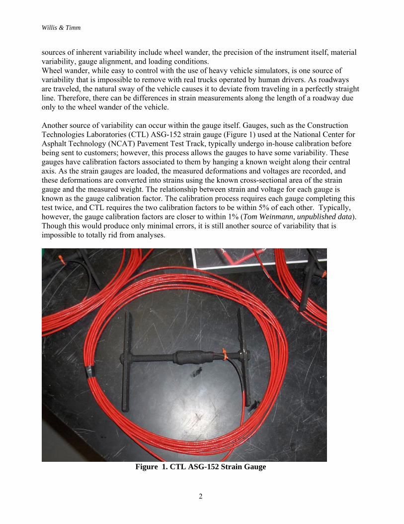
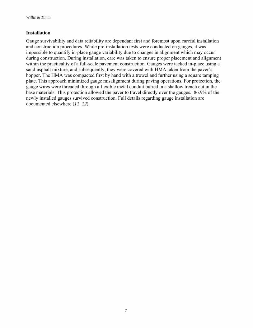
sources of inherent variability include wheel wander, the precision of the instrument itself, material variability, gauge alignment, and loading conditions. Wheel wander, while easy to control with the use of heavy vehicle simulators, is one source of variability that is impossible to remove with real trucks operated by human drivers. As roadways are traveled, the natural sway of the vehicle causes it to deviate from traveling in a perfectly straight line. Therefore, there can be differences in strain measurements along the length of a roadway due only to the wheel wander of the vehicle. Another source of variability can occur within the gauge itself. Gauges, such as the Construction Technologies Laboratories (CTL) ASG-152 strain gauge (Figure 1) used at the National Center for Asphalt Technology (NCAT) Pavement Test Track, typically undergo in-house calibration before being sent to customers; however, this process allows the gauges to have some variability. These gauges have calibration factors associated to them by hanging a known weight along their central axis. As the strain gauges are loaded, the measured deformations and voltages are recorded, and these deformations are converted into strains using the known cross-sectional area of the strain gauge and the measured weight. The relationship between strain and voltage for each gauge is known as the gauge calibration factor. The calibration process requires each gauge completing this test twice, and CTL requires the two calibration factors to be within 5% of each other. Typically, however, the gauge calibration factors are closer to within 1% (Tom Weinmann, unpublished data). Though this would produce only minimal errors, it is still another source of variability that is impossible to totally rid from analyses.
Figure 1. CTL ASG-152 Strain Gauge
Willis & Timm
3
Material variability is a third potential source for precision error in embedded roadway instrumentation. Although great care is taken to ensure uniform pavement layers are placed during construction by the contractor, variations can and do occur. Duplicate gauges placed in two different areas can produce different responses due to material variability. For example, a difference in stiffness between two locations would result in a difference in measured strains. While one might assume that the difference could be due to wheel wander or some other phenomenon, in all actuality, the pavement structure caused the differences in strain readings. While material uniformity is important, one must also consider that slight deviations in layer thicknesses could cause variation in replicate strain measurements. Strain gauges are typically oriented in one of two directions: longitudinal (with traffic) or transversely (perpendicular to traffic). If two gauges are designed to measure the transverse strain under the center of the wheelpath, both gauges need to be placed with the same transverse offset from the edge stripe and perpendicular to the wheelpath. Great care must be taken to complete proper placement because poorly placed gauges will not measure the same strain levels. A final source of variability comes from the dynamics of vehicular loading. Vehicle dynamic effects in an instrumented section create the possibility that a “direct hit” might not occur at the location of the instrument. Vehicle bounce could prevent the tires from being in full-contact with the pavement directly over the gauge. The gauge, in turn, would read a smaller strain value at that point than if another gauge were to receive a direct hit.
Quantifying Variability
Little research has been published quantifying the variability in pavement instrumentation despite its prevalent use in research today. In the summer of 2000, the South Dakota Department of Transportation instrumented four flexible pavements with four longitudinal strain gauges at the bottom of the asphalt layer to study the impact of off-road equipment on flexible pavements. The team also placed pressure cells at the top of the subgrade and base layer. With this instrumentation in place, the research team also investigated the repeatability of its pavement instrumentation (8). Variability was examined from the instrumented pavements on five replicate runs of each loading scenario in the test. Replicate data from the pressure cells and strain gauges were analyzed for repeatability and averages. Pressure repeatability was found to be good, having a coefficient of variation less than five percent. On the other hand, strain measurements were found to be more variable than pressure measurements. Upon careful review of the variability factors, including wheel wander and vehicle bounce, it was determined a ±30% difference in measured strains from a single gauge could be expected (8). Another experiment was conducted using the thin asphalt pavements at the ROADHOG program at the University of Arkansas. One hundred ten sensors, which included hydraulic total earth pressure cells, standard pressure cells, H-strain gauges, and foil strain gauges, were installed in pavement sections for study. Duplicate strain gauges were placed in each section to measure transverse and longitudinal strain. Measurements were collected for the first six months of the newly constructed experiment (9).
Willis & Timm
4
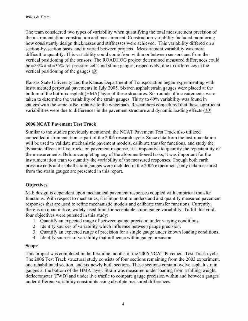
The team considered two types of variability when quantifying the total measurement precision of the instrumentation: construction and measurement. Construction variability included monitoring how consistently design thicknesses and stiffnesses were achieved. This variability differed on a section-by-section basis, and it varied between projects. Measurement variability was more difficult to quantify. This variability could come from within or between sensors and from the vertical positioning of the sensors. The ROADHOG project determined measured differences could be ±23% and ±35% for pressure cells and strain gauges, respectively, due to differences in the vertical positioning of the gauges (9). Kansas State University and the Kansas Department of Transportation began experimenting with instrumented perpetual pavements in July 2005. Sixteen asphalt strain gauges were placed at the bottom of the hot-mix asphalt (HMA) layer of these structures. Six rounds of measurements were taken to determine the variability of the strain gauges. Thirty to 60% variability was found in gauges with the same offset relative to the wheelpath. Researchers conjectured that these significant variabilities were due to differences in the pavement structure and dynamic loading effects (10).
2006 NCAT Pavement Test Track
Similar to the studies previously mentioned, the NCAT Pavement Test Track also utilized embedded instrumentation as part of the 2006 research cycle. Since data from the instrumentation will be used to validate mechanistic pavement models, calibrate transfer functions, and study the dynamic effects of live trucks on pavement response, it is imperative to quantify the repeatability of the measurements. Before completing any of the aforementioned tasks, it was important for the instrumentation team to quantify the variability of the measured responses. Though both earth pressure cells and asphalt strain gauges were included in the 2006 experiment, only data measured from the strain gauges are presented in this report.
Objectives
M-E design is dependent upon mechanical pavement responses coupled with empirical transfer functions. With respect to mechanics, it is important to understand and quantify measured pavement responses that are used to refine mechanistic models and calibrate transfer functions. Currently, there is no quantitative, widely-used limit for acceptable strain gauge variability. To fill this void, four objectives were pursued in this study:
1. Quantify an expected range of between gauge precision under varying conditions. 2. Identify sources of variability which influence between gauge precision. 3. Quantify an expected range of precision for a single gauge under known loading conditions. 4. Identify sources of variability that influence within gauge precision.
Scope
This project was completed in the first nine months of the 2006 NCAT Pavement Test Track cycle. The 2006 Test Track structural study consists of four sections remaining from the 2003 experiment, one rehabilitated section, and six newly built sections. These sections contain twelve asphalt strain gauges at the bottom of the HMA layer. Strain was measured under loading from a falling-weight deflectometer (FWD) and under live traffic to compare gauge precision within and between gauges under different variability constraints using absolute measured differences.
Willis & Timm
5
CHAPTER 2 – TEST FACILITY AND INSTRUMENTATION
Test Sections
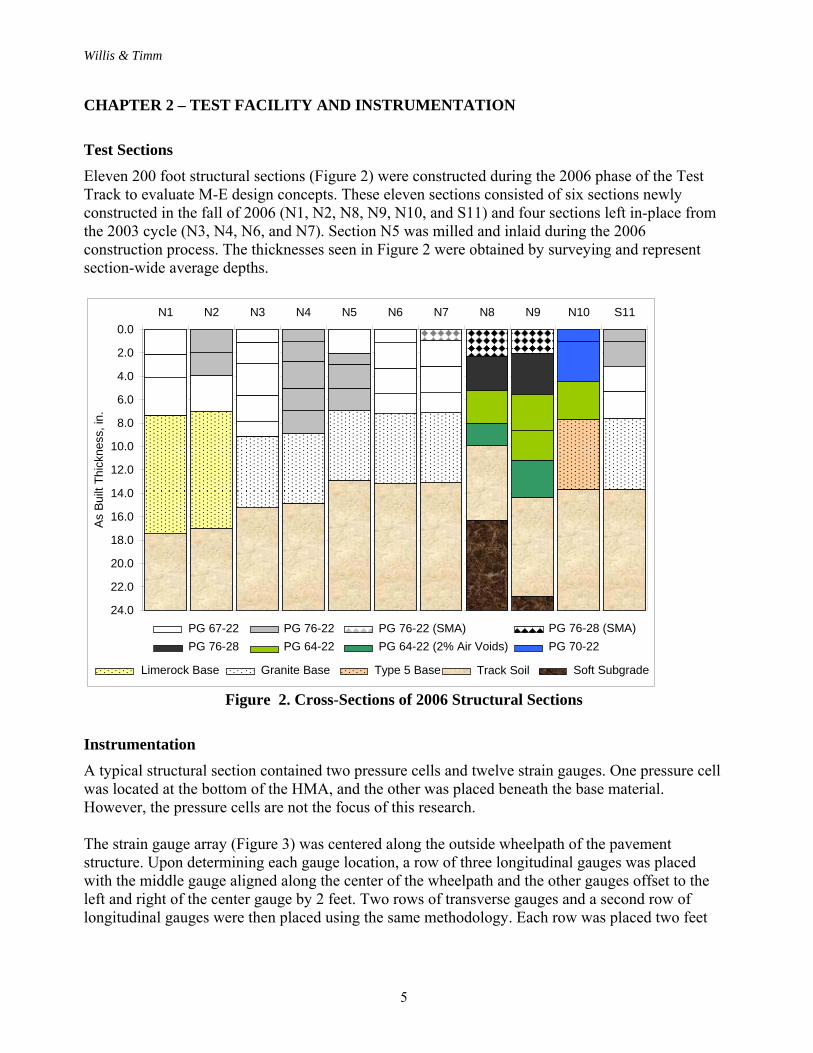
Eleven 200 foot structural sections (Figure 2) were constructed during the 2006 phase of the Test Track to evaluate M-E design concepts. These eleven sections consisted of six sections newly constructed in the fall of 2006 (N1, N2, N8, N9, N10, and S11) and four sections left in-place from the 2003 cycle (N3, N4, N6, and N7). Section N5 was milled and inlaid during the 2006 construction process. The thicknesses seen in Figure 2 were obtained by surveying and represent section-wide average depths.
0.0
2.0
4.0
6.0
8.0
10.0
12.0
14.0
16.0
18.0
20.0
22.0
24.0
N1 N2 N3 N4 N5 N6 N7 N8 N9 N10 S11
As
Bu
ilt T
hick
nes
s, in
.
PG 67-22 PG 76-22 PG 76-22 (SMA) PG 76-28 (SMA)
PG 76-28 PG 64-22 PG 64-22 (2% Air Voids) PG 70-22
Limerock Base Granite Base Type 5 Base Track Soil Soft Subgrade
Figure 2. Cross-Sections of 2006 Structural Sections
Instrumentation
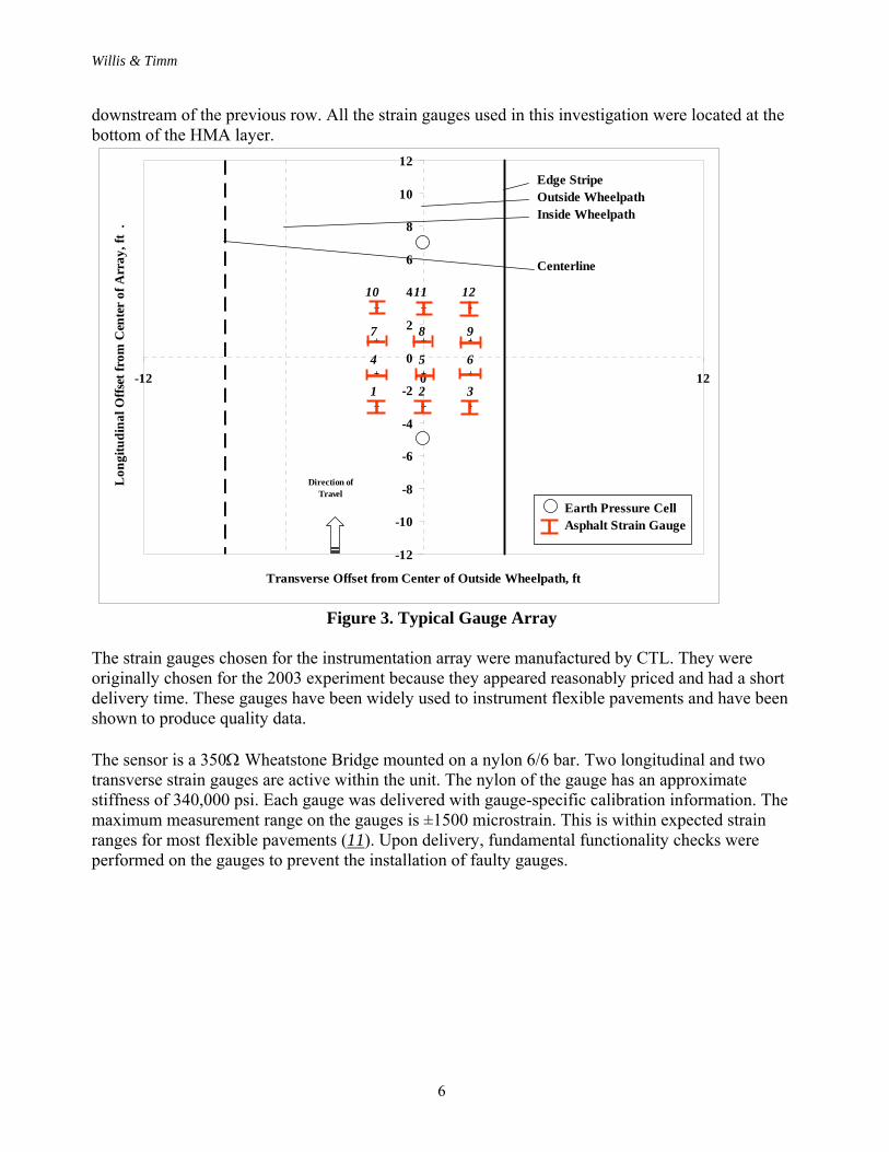
A typical structural section contained two pressure cells and twelve strain gauges. One pressure cell was located at the bottom of the HMA, and the other was placed beneath the base material. However, the pressure cells are not the focus of this research. The strain gauge array (Figure 3) was centered along the outside wheelpath of the pavement structure. Upon determining each gauge location, a row of three longitudinal gauges was placed with the middle gauge aligned along the center of the wheelpath and the other gauges offset to the left and right of the center gauge by 2 feet. Two rows of transverse gauges and a second row of longitudinal gauges were then placed using the same methodology. Each row was placed two feet
Willis & Timm
6
downstream of the previous row. All the strain gauges used in this investigation were located at the bottom of the HMA layer.
-12
-10
-8
-6
-4
-2
0
2
4
6
8
10
12
-12 0 12
Transverse Offset from Center of Outside Wheelpath, ft
Lon
gitu
din
al O
ffse
t fr
om C
ente
r of
Arr
ay, f
t .
Earth Pressure CellAsphalt Strain Gauge
Edge StripeOutside WheelpathInside Wheelpath
Centerline
Direction of Travel
1 2 3
4 5 6
7 8 9
10 11 12
Figure 3. Typical Gauge Array
The strain gauges chosen for the instrumentation array were manufactured by CTL. They were originally chosen for the 2003 experiment because they appeared reasonably priced and had a short delivery time. These gauges have been widely used to instrument flexible pavements and have been shown to produce quality data. The sensor is a 350 Wheatstone Bridge mounted on a nylon 6/6 bar. Two longitudinal and two transverse strain gauges are active within the unit. The nylon of the gauge has an approximate stiffness of 340,000 psi. Each gauge was delivered with gauge-specific calibration information. The maximum measurement range on the gauges is ±1500 microstrain. This is within expected strain ranges for most flexible pavements (11). Upon delivery, fundamental functionality checks were performed on the gauges to prevent the installation of faulty gauges.
Willis & Timm
7
Installation
Gauge survivability and data reliability are dependant first and foremost upon careful installation and construction procedures. While pre-installation tests were conducted on gauges, it was impossible to quantify in-place gauge variability due to changes in alignment which may occur during construction. During installation, care was taken to ensure proper placement and alignment within the practicality of a full-scale pavement construction. Gauges were tacked in-place using a sand-asphalt mixture, and subsequently, they were covered with HMA taken from the paver’s hopper. The HMA was compacted first by hand with a trowel and further using a square tamping plate. This approach minimized gauge misalignment during paving operations. For protection, the gauge wires were threaded through a flexible metal conduit buried in a shallow trench cut in the base materials. This protection allowed the paver to travel directly over the gauges. 86.9% of the newly installed gauges survived construction. Full details regarding gauge installation are documented elsewhere (11, 12).
Willis & Timm
8
CHAPTER 3 – BETWEEN GAUGE PRECISION UNDER LIVE TRAFFIC The gauge array portrayed in the previous chapter (Figure 2) has many practical applications; however, two are essential to the study of between gauge precision. First, since the gauge array is centered along the outside wheelpath at a facility where drivers are used to traffic the pavement, wheel wander can be captured by the gauge array. If a truck was tracking closer to the edge of the pavement, the outside gauges would be able to receive the more direct hit. Second, each strain gauge is duplicated. In other words, each strain gauge has one other gauge with the same orientation, depth, and transverse offset from the edge stripe. For example, gauges one and ten from Figure 3 form a longitudinal, left of the wheelpath pair. Some strain gauges did not survive the construction process, and the redundancy of gauges allows for data still to be collected at the same offset and orientation. While redundancy and wander are two reasons for the gauge array design, using duplicate gauges enables a functionality check to be made. If two gauges have the same depth, transverse location, and orientation, then the two strain gauges should measure similar strains in the pavement structure. If this is not the case, barring some inherent variability, then a gauge may not be functioning properly or may have become misaligned.
Data Acquisition and Processing
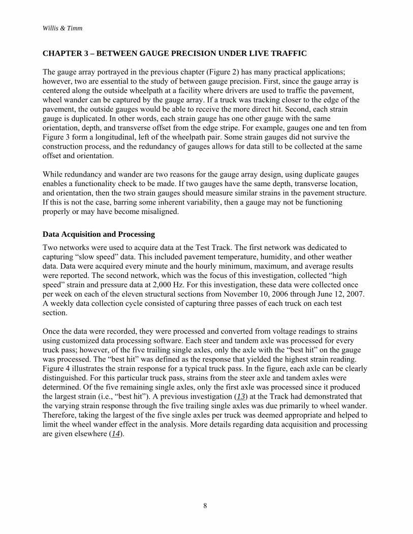
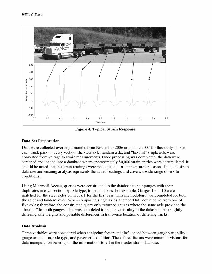
Two networks were used to acquire data at the Test Track. The first network was dedicated to capturing “slow speed” data. This included pavement temperature, humidity, and other weather data. Data were acquired every minute and the hourly minimum, maximum, and average results were reported. The second network, which was the focus of this investigation, collected “high speed” strain and pressure data at 2,000 Hz. For this investigation, these data were collected once per week on each of the eleven structural sections from November 10, 2006 through June 12, 2007. A weekly data collection cycle consisted of capturing three passes of each truck on each test section. Once the data were recorded, they were processed and converted from voltage readings to strains using customized data processing software. Each steer and tandem axle was processed for every truck pass; however, of the five trailing single axles, only the axle with the “best hit” on the gauge was processed. The “best hit” was defined as the response that yielded the highest strain reading. Figure 4 illustrates the strain response for a typical truck pass. In the figure, each axle can be clearly distinguished. For this particular truck pass, strains from the steer axle and tandem axles were determined. Of the five remaining single axles, only the first axle was processed since it produced the largest strain (i.e., “best hit”). A previous investigation (13) at the Track had demonstrated that the varying strain response through the five trailing single axles was due primarily to wheel wander. Therefore, taking the largest of the five single axles per truck was deemed appropriate and helped to limit the wheel wander effect in the analysis. More details regarding data acquisition and processing are given elsewhere (14).
Willis & Timm
9
Figure 4. Typical Strain Response
Data Set Preparation
Data were collected over eight months from November 2006 until June 2007 for this analysis. For each truck pass on every section, the steer axle, tandem axle, and “best hit” single axle were converted from voltage to strain measurements. Once processing was completed, the data were screened and loaded into a database where approximately 80,000 strain entries were accumulated. It should be noted that the strain readings were not adjusted for temperature or season. Thus, the strain database and ensuing analysis represents the actual readings and covers a wide range of in situ conditions. Using Microsoft Access, queries were constructed in the database to pair gauges with their duplicates in each section by axle type, truck, and pass. For example, Gauges 1 and 10 were matched for the steer axles on Truck 1 for the first pass. This methodology was completed for both the steer and tandem axles. When comparing single axles, the “best hit” could come from one of five axles; therefore, the constructed query only returned gauges where the same axle provided the “best hit” for both gauges. This was completed to reduce variability in the dataset due to slightly differing axle weights and possible differences in transverse location of differing trucks.
Data Analysis
Three variables were considered when analyzing factors that influenced between gauge variability: gauge orientation, axle type, and pavement condition. These three factors were natural divisions for data manipulation based upon the information stored in the master strain database.
Right Gauge
-200
-100
0
100
200
300
400
500
0.5 0.7 0.9 1.1 1.3 1.5 1.7 1.9 2.1 2.3 2.5
Time, sec
Long
tidin
al M
icro
stra
in
Willis & Timm
10
Both percent differences and absolute differences were considered for this investigation; however, percent differences can bias the data towards one of the two measurements while absolute differences contain no bias. It is simply the difference between two readings. Therefore, for this analysis, measured differences were calculated by subtracting readings between paired gauges and then determining the absolute value.
Gauge Orientation Comparisons
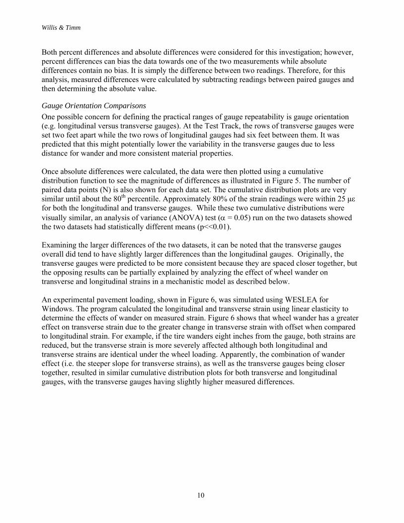
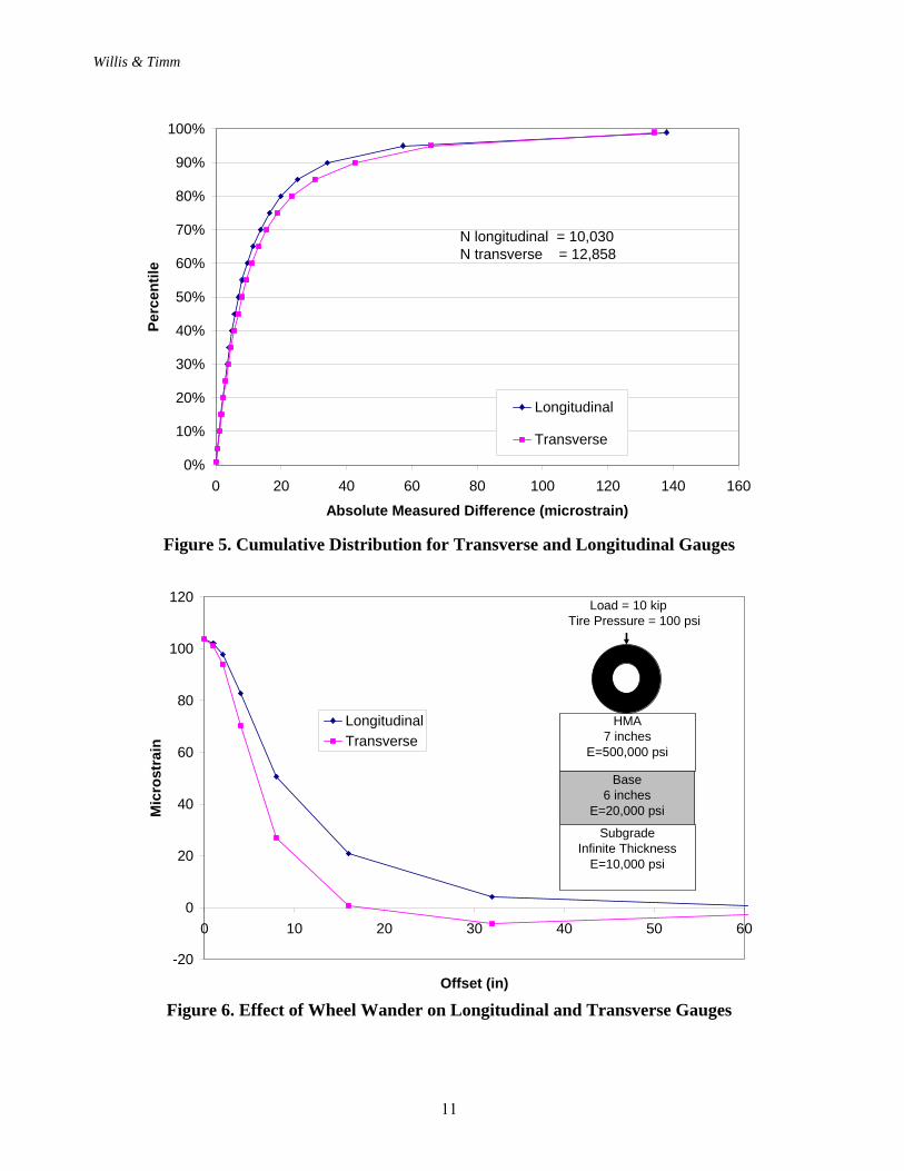
One possible concern for defining the practical ranges of gauge repeatability is gauge orientation (e.g. longitudinal versus transverse gauges). At the Test Track, the rows of transverse gauges were set two feet apart while the two rows of longitudinal gauges had six feet between them. It was predicted that this might potentially lower the variability in the transverse gauges due to less distance for wander and more consistent material properties. Once absolute differences were calculated, the data were then plotted using a cumulative distribution function to see the magnitude of differences as illustrated in Figure 5. The number of paired data points (N) is also shown for each data set. The cumulative distribution plots are very similar until about the 80th percentile. Approximately 80% of the strain readings were within 25 με for both the longitudinal and transverse gauges. While these two cumulative distributions were visually similar, an analysis of variance (ANOVA) test ( = 0.05) run on the two datasets showed the two datasets had statistically different means (p<<0.01). Examining the larger differences of the two datasets, it can be noted that the transverse gauges overall did tend to have slightly larger differences than the longitudinal gauges. Originally, the transverse gauges were predicted to be more consistent because they are spaced closer together, but the opposing results can be partially explained by analyzing the effect of wheel wander on transverse and longitudinal strains in a mechanistic model as described below. An experimental pavement loading, shown in Figure 6, was simulated using WESLEA for Windows. The program calculated the longitudinal and transverse strain using linear elasticity to determine the effects of wander on measured strain. Figure 6 shows that wheel wander has a greater effect on transverse strain due to the greater change in transverse strain with offset when compared to longitudinal strain. For example, if the tire wanders eight inches from the gauge, both strains are reduced, but the transverse strain is more severely affected although both longitudinal and transverse strains are identical under the wheel loading. Apparently, the combination of wander effect (i.e. the steeper slope for transverse strains), as well as the transverse gauges being closer together, resulted in similar cumulative distribution plots for both transverse and longitudinal gauges, with the transverse gauges having slightly higher measured differences.
Willis & Timm
11
0%
10%
20%
30%
40%
50%
60%
70%
80%
90%
100%
0 20 40 60 80 100 120 140 160
Absolute Measured Difference (microstrain)
Per
cen
tile
Longitudinal
Transverse
N longitudinal = 10,030N transverse = 12,858
Figure 5. Cumulative Distribution for Transverse and Longitudinal Gauges
-20
0
20
40
60
80
100
120
0 10 20 30 40 50 60
Offset (in)
Mic
rost
rain
Longitudinal
Transverse
HMA7 inches
E=500,000 psi
SubgradeInfinite Thickness
E=10,000 psi
Base6 inches
E=20,000 psi
Load = 10 kipTire Pressure = 100 psi
Figure 6. Effect of Wheel Wander on Longitudinal and Transverse Gauges
Willis & Timm
12
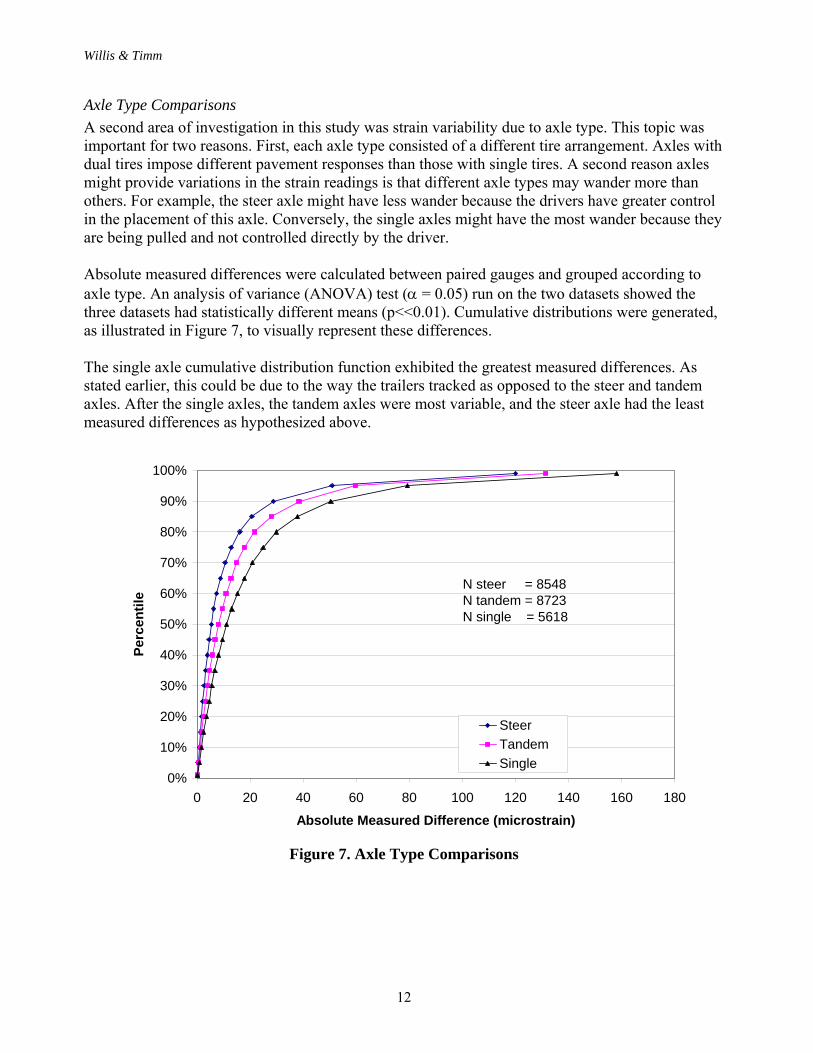
Axle Type Comparisons
A second area of investigation in this study was strain variability due to axle type. This topic was important for two reasons. First, each axle type consisted of a different tire arrangement. Axles with dual tires impose different pavement responses than those with single tires. A second reason axles might provide variations in the strain readings is that different axle types may wander more than others. For example, the steer axle might have less wander because the drivers have greater control in the placement of this axle. Conversely, the single axles might have the most wander because they are being pulled and not controlled directly by the driver. Absolute measured differences were calculated between paired gauges and grouped according to axle type. An analysis of variance (ANOVA) test ( = 0.05) run on the two datasets showed the three datasets had statistically different means (p<<0.01). Cumulative distributions were generated, as illustrated in Figure 7, to visually represent these differences. The single axle cumulative distribution function exhibited the greatest measured differences. As stated earlier, this could be due to the way the trailers tracked as opposed to the steer and tandem axles. After the single axles, the tandem axles were most variable, and the steer axle had the least measured differences as hypothesized above.
0%
10%
20%
30%
40%
50%
60%
70%
80%
90%
100%
0 20 40 60 80 100 120 140 160 180
Absolute Measured Difference (microstrain)
Per
cen
tile
Steer
Tandem
Single
N steer = 8548N tandem = 8723N single = 5618
Figure 7. Axle Type Comparisons
Willis & Timm
13
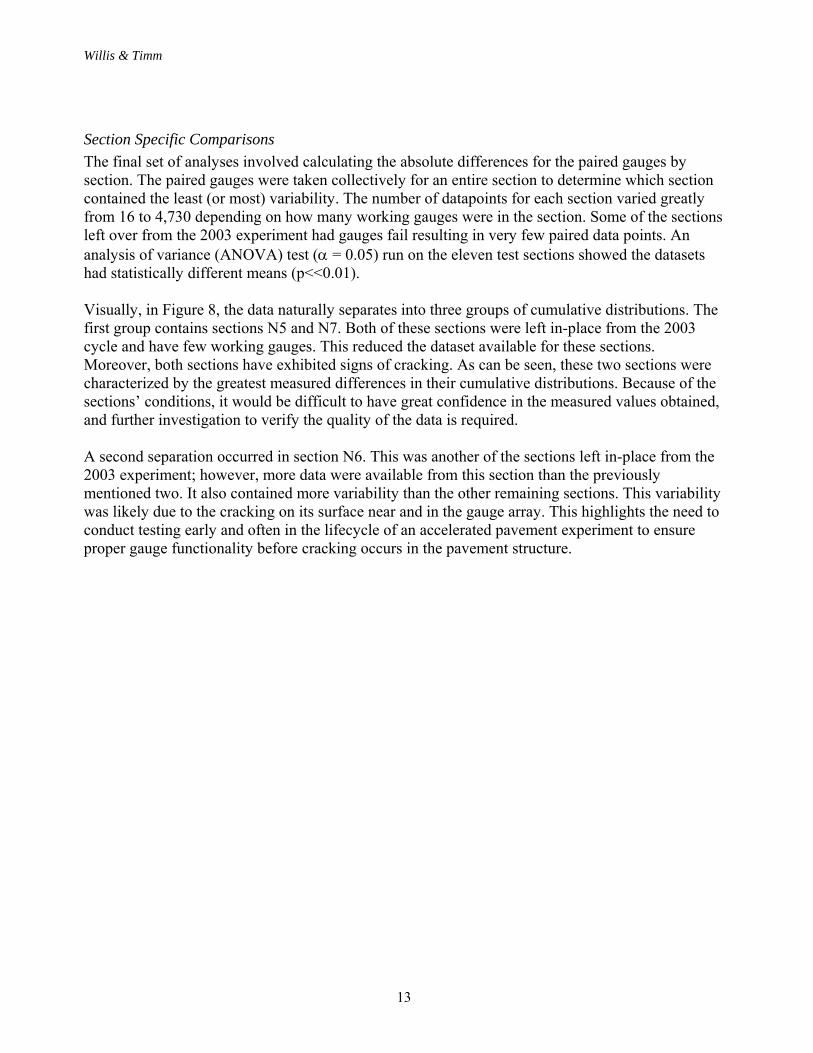
Section Specific Comparisons
The final set of analyses involved calculating the absolute differences for the paired gauges by section. The paired gauges were taken collectively for an entire section to determine which section contained the least (or most) variability. The number of datapoints for each section varied greatly from 16 to 4,730 depending on how many working gauges were in the section. Some of the sections left over from the 2003 experiment had gauges fail resulting in very few paired data points. An analysis of variance (ANOVA) test ( = 0.05) run on the eleven test sections showed the datasets had statistically different means (p<<0.01). Visually, in Figure 8, the data naturally separates into three groups of cumulative distributions. The first group contains sections N5 and N7. Both of these sections were left in-place from the 2003 cycle and have few working gauges. This reduced the dataset available for these sections. Moreover, both sections have exhibited signs of cracking. As can be seen, these two sections were characterized by the greatest measured differences in their cumulative distributions. Because of the sections’ conditions, it would be difficult to have great confidence in the measured values obtained, and further investigation to verify the quality of the data is required. A second separation occurred in section N6. This was another of the sections left in-place from the 2003 experiment; however, more data were available from this section than the previously mentioned two. It also contained more variability than the other remaining sections. This variability was likely due to the cracking on its surface near and in the gauge array. This highlights the need to conduct testing early and often in the lifecycle of an accelerated pavement experiment to ensure proper gauge functionality before cracking occurs in the pavement structure.
Willis & Timm
14
0%
10%
20%
30%
40%
50%
60%
70%
80%
90%
100%
0 100 200 300 400 500
Absolute Measured Difference (microstrain)
Per
cen
tile
N1N2N3N4N5N6N7N8N9N10S11
Data PointsN1 = 4730N2 = 4206N3 = 25N4 = 612N5 = 23N6 = 716N7 = 16N8 = 4112N9 = 2254N10 = 1829S11 = 4232
Figure 8. Sectional Comparison
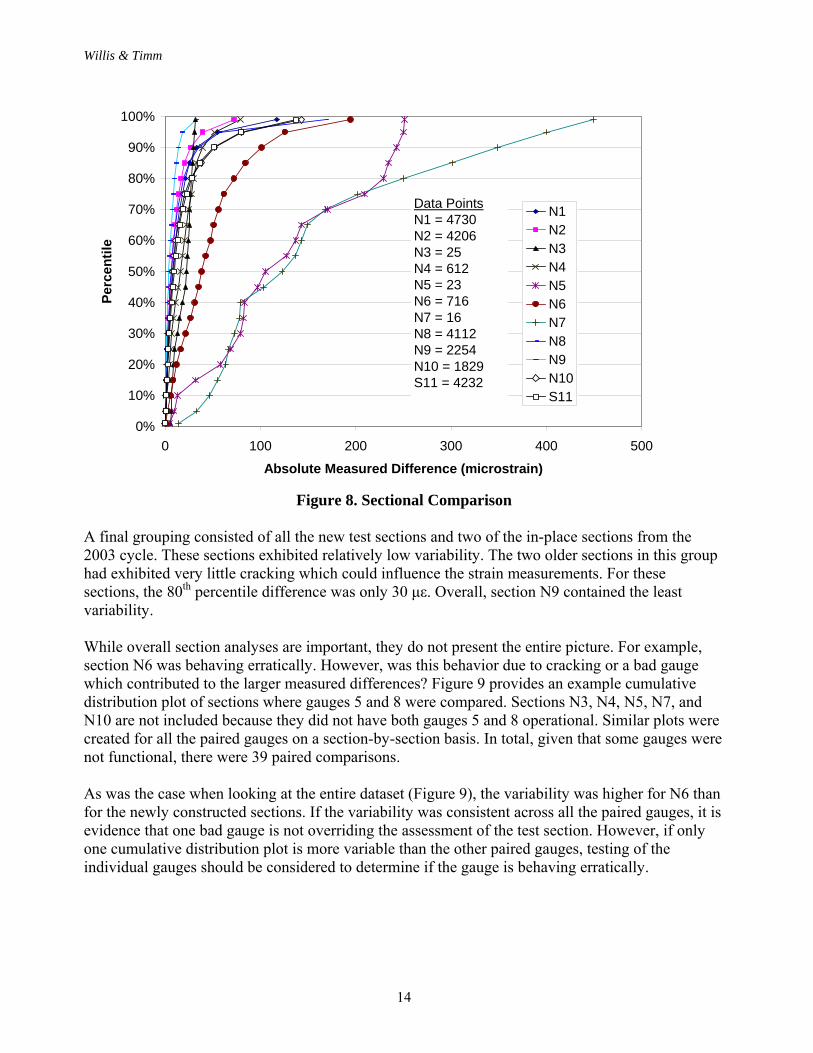
A final grouping consisted of all the new test sections and two of the in-place sections from the 2003 cycle. These sections exhibited relatively low variability. The two older sections in this group had exhibited very little cracking which could influence the strain measurements. For these sections, the 80th percentile difference was only 30 με. Overall, section N9 contained the least variability. While overall section analyses are important, they do not present the entire picture. For example, section N6 was behaving erratically. However, was this behavior due to cracking or a bad gauge which contributed to the larger measured differences? Figure 9 provides an example cumulative distribution plot of sections where gauges 5 and 8 were compared. Sections N3, N4, N5, N7, and N10 are not included because they did not have both gauges 5 and 8 operational. Similar plots were created for all the paired gauges on a section-by-section basis. In total, given that some gauges were not functional, there were 39 paired comparisons. As was the case when looking at the entire dataset (Figure 9), the variability was higher for N6 than for the newly constructed sections. If the variability was consistent across all the paired gauges, it is evidence that one bad gauge is not overriding the assessment of the test section. However, if only one cumulative distribution plot is more variable than the other paired gauges, testing of the individual gauges should be considered to determine if the gauge is behaving erratically.
Willis & Timm
15
0
10
20
30
40
50
60
70
80
90
100
0 100 200 300 400 500 600
Absolute Difference (microstrains)
Per
cen
tile
N1N2N6N9S11
Figure 9. Comparison of Gauges 5 and 8
The majority of the cumulative distribution functions for the individually paired gauges were similar to the plots of sections N1 and N2 in Figure 9. Very little variation was exhibited until around the 80th percentile. If the 80th percentile was set as a benchmark, 32 of 39 paired gauge sets had absolute measured differences less than 30 με. Since this strain value coincides with the 80th percentile of gauges functioning in non-cracked test sections (Figure 8), a 30 με absolute difference at the 80th percentile was set as the benchmark for the Test Track for between gauge precision.
Summary
When embedded pavement instrumentation is incorporated into a study, one must first be aware of their advantages and limitations. When trying to measure the same strain on duplicate gauges, the measurement variability is caused by material variability, wheel wander, and instrument precision. The findings in this chapter led to better understanding of the gauges measurement variability. The following conclusions are based on between gauge variability measured at the Test Track under dynamic loading:
Transverse gauges and single axle measurements tend to show more variability than their counterparts because of the effects of wheel wander.
Cracking introduces noise into pavement measurements.Measurements should be conducted early in a pavement’s life to capture strain levels before cracking introduces more variability into the data.
From this analysis at the Test Track, it was determined a strain of 30 με could be used as a suitable threshold for evaluating the reliability of strain measurements. Paired gauges should be within 30 με in order to be used for analysis purposes. If the absolute differences

Willis & Timm
16
obtained from paired gauges fall outside of this threshold, forensics will be conducted to determine why the gauge is outside of this range.
One possible method for testing a gauge for valid readings is using an FWD to drop a consistent load concentrically onto the gauge. The strain readings produced from this impact load should be relatively precise. The FWD loading scenario removes material differences and wheel wander variability and focuses on the precision of the instrument itself. But what is the allowable precision for one gauge? The next chapter analyzed what an acceptable range of precision is for one gauge at the Test Track.
Willis & Timm
17
CHAPTER 4 – WITHIN GAUGE REPEATABILITY UNDER FALLING WEIGHT DEFLECTOMETER LOADING As previously discussed, there are numerous sources of measurement variability associated with capturing pavement responses under trafficking. While the use of live trafficking does not allow these inconsistencies to be negated, specialized testing can reduce the sources of variability contributing to potentially erroneously measured responses. When pavements are trafficked by vehicles operated by drivers, it is impossible to totally rid the responses captured of vehicle bounce and wheel wander which both contribute significantly to the measured strain response of the gauges. When measuring between gauges, it is unlikely that the materials will be the same in both thickness and stiffness so that the strain measurements are not affected. However, if a known load is placed concentrically on top of a single gauge multiple times, the variability of the single gauge could be studied with primarily the precision of the instrument affecting the variability of the measurements.
Methodology
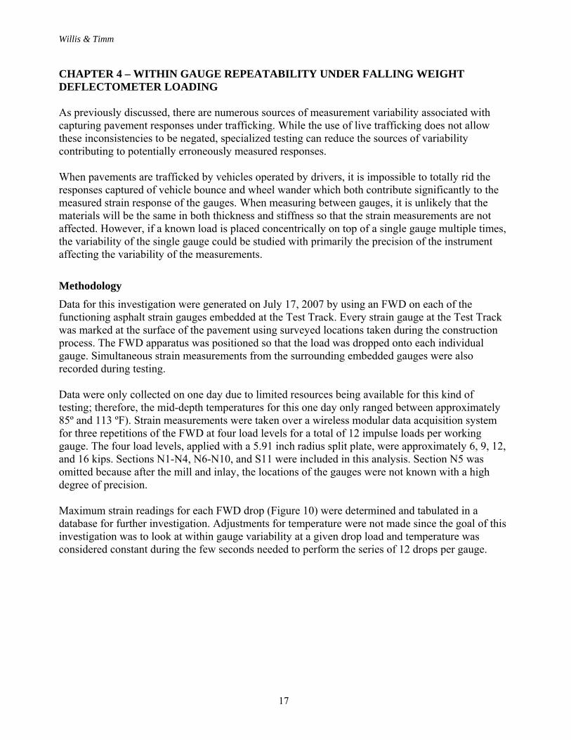
Data for this investigation were generated on July 17, 2007 by using an FWD on each of the functioning asphalt strain gauges embedded at the Test Track. Every strain gauge at the Test Track was marked at the surface of the pavement using surveyed locations taken during the construction process. The FWD apparatus was positioned so that the load was dropped onto each individual gauge. Simultaneous strain measurements from the surrounding embedded gauges were also recorded during testing. Data were only collected on one day due to limited resources being available for this kind of testing; therefore, the mid-depth temperatures for this one day only ranged between approximately 85º and 113 ºF). Strain measurements were taken over a wireless modular data acquisition system for three repetitions of the FWD at four load levels for a total of 12 impulse loads per working gauge. The four load levels, applied with a 5.91 inch radius split plate, were approximately 6, 9, 12, and 16 kips. Sections N1-N4, N6-N10, and S11 were included in this analysis. Section N5 was omitted because after the mill and inlay, the locations of the gauges were not known with a high degree of precision. Maximum strain readings for each FWD drop (Figure 10) were determined and tabulated in a database for further investigation. Adjustments for temperature were not made since the goal of this investigation was to look at within gauge variability at a given drop load and temperature was considered constant during the few seconds needed to perform the series of 12 drops per gauge.
Willis & Timm
18
-25
25
75
125
175
225
275
21500 21600 21700 21800 21900 22000 22100 22200 22300 22400 22500
Mic
rost
rain
Maximum Strain
Figure 10. Maximum Strain Example
Data Analysis
The FWD loaded each strain gauge with three repetitions of four different loads for a total of 12 strain responses. At each load level, the absolute measured difference between the maximum and minimum strain readings was determined. The following sets of analysis use the absolute difference as a primary measure of within-gauge precision with an additional investigation using percent differences to examine the effect of strain magnitude.
Gauge Orientation Comparisons
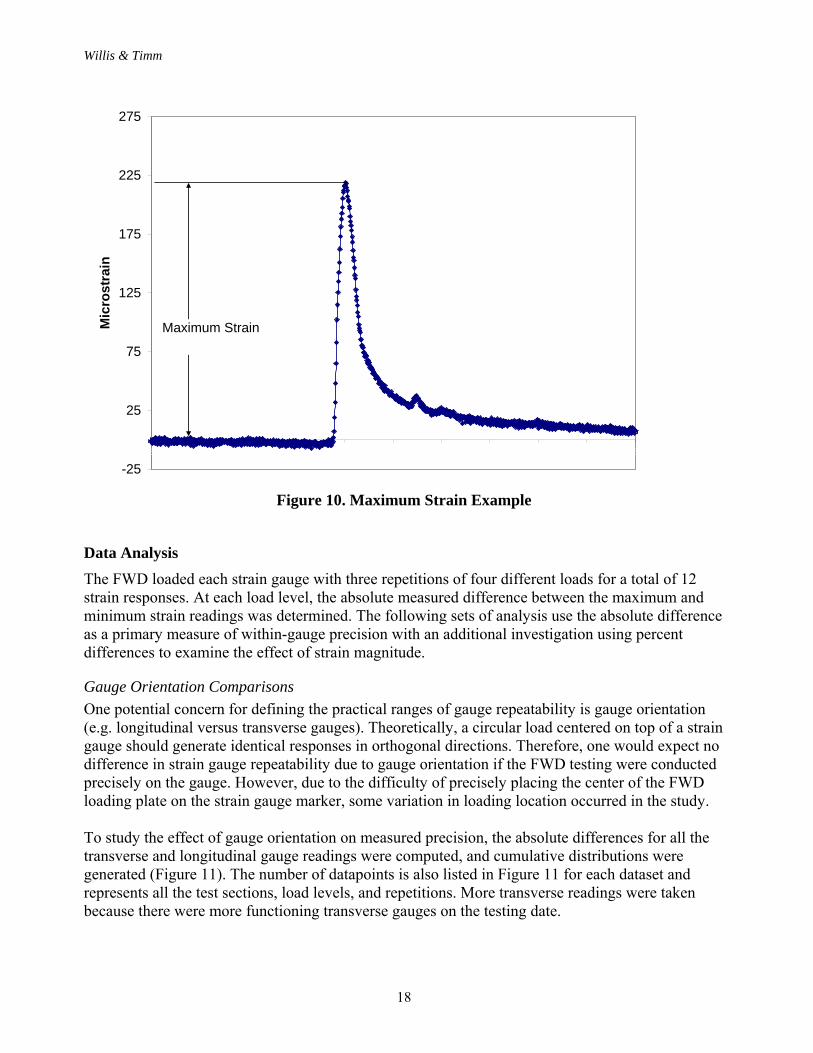
One potential concern for defining the practical ranges of gauge repeatability is gauge orientation (e.g. longitudinal versus transverse gauges). Theoretically, a circular load centered on top of a strain gauge should generate identical responses in orthogonal directions. Therefore, one would expect no difference in strain gauge repeatability due to gauge orientation if the FWD testing were conducted precisely on the gauge. However, due to the difficulty of precisely placing the center of the FWD loading plate on the strain gauge marker, some variation in loading location occurred in the study. To study the effect of gauge orientation on measured precision, the absolute differences for all the transverse and longitudinal gauge readings were computed, and cumulative distributions were generated (Figure 11). The number of datapoints is also listed in Figure 11 for each dataset and represents all the test sections, load levels, and repetitions. More transverse readings were taken because there were more functioning transverse gauges on the testing date.
Willis & Timm
19
As seen in Figure 11, virtually no difference is observed between the cumulative distributions until the 90th percentile. Small discrepancies occur at the 55th and 60th percentile, but in both cases, the differences in the plots are less than 0.3 με. At the 85th percentile, both the transverse and longitudinal strain gauges had absolute differences of approximately 6 με. After this point, the longitudinal gauges tended to show slightly more variability. These values might be the result of outliers which could be due to data processing errors or voltage spikes. The outliers did not come from the same gauge; therefore, it is unlikely that a single gauge is at fault for the larger differences. To statistically validate the similarities between the cumulative distributions, a Kolmogorov-Smirnoff (K-S) test ( = 0.05) was performed on the two sets of strain measurements. A K-S test checks for statistical distinctions between the cumulative distributions of two datasets (15). A K-S test did not detect statistical differences (p = 0.429). Knowing this, it can be stated that 90% of the readings, covering all the test sections and load levels, generated differences less than 7 με and was not dependent upon gauge orientation.
0%
10%
20%
30%
40%
50%
60%
70%
80%
90%
100%
0 5 10 15 20 25
Absolute Difference, microstrain
Pe
rcen
tile
Transverse
Longitudinal
Transverse = 956Longitudinal = 688
Figure 11. Cumulative Distributions for Longitudinal and Transverse Gauges
Load Level Comparisons
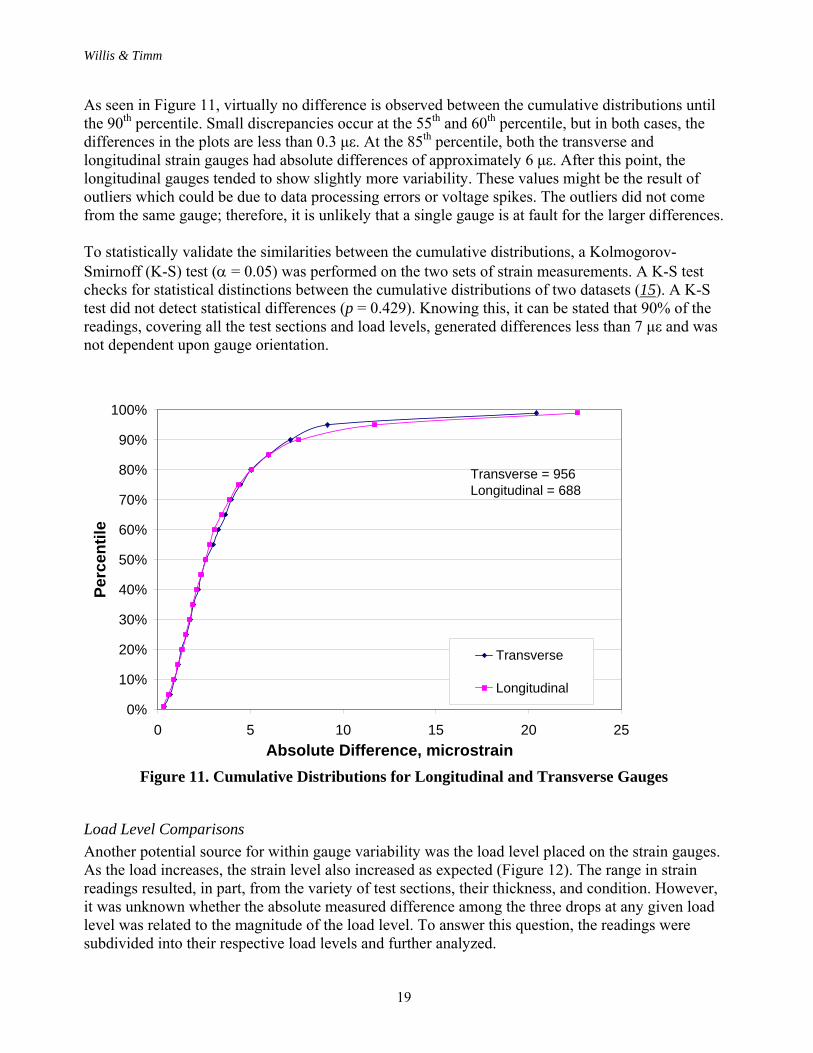
Another potential source for within gauge variability was the load level placed on the strain gauges. As the load increases, the strain level also increased as expected (Figure 12). The range in strain readings resulted, in part, from the variety of test sections, their thickness, and condition. However, it was unknown whether the absolute measured difference among the three drops at any given load level was related to the magnitude of the load level. To answer this question, the readings were subdivided into their respective load levels and further analyzed.
Willis & Timm
20
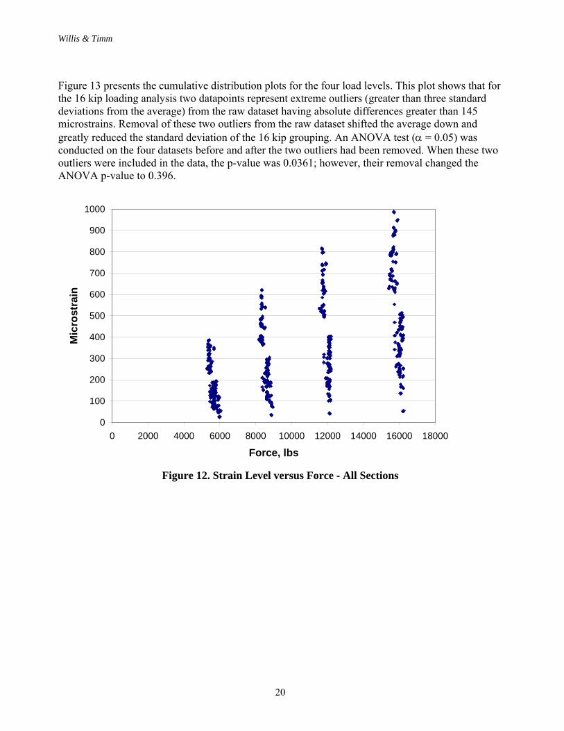
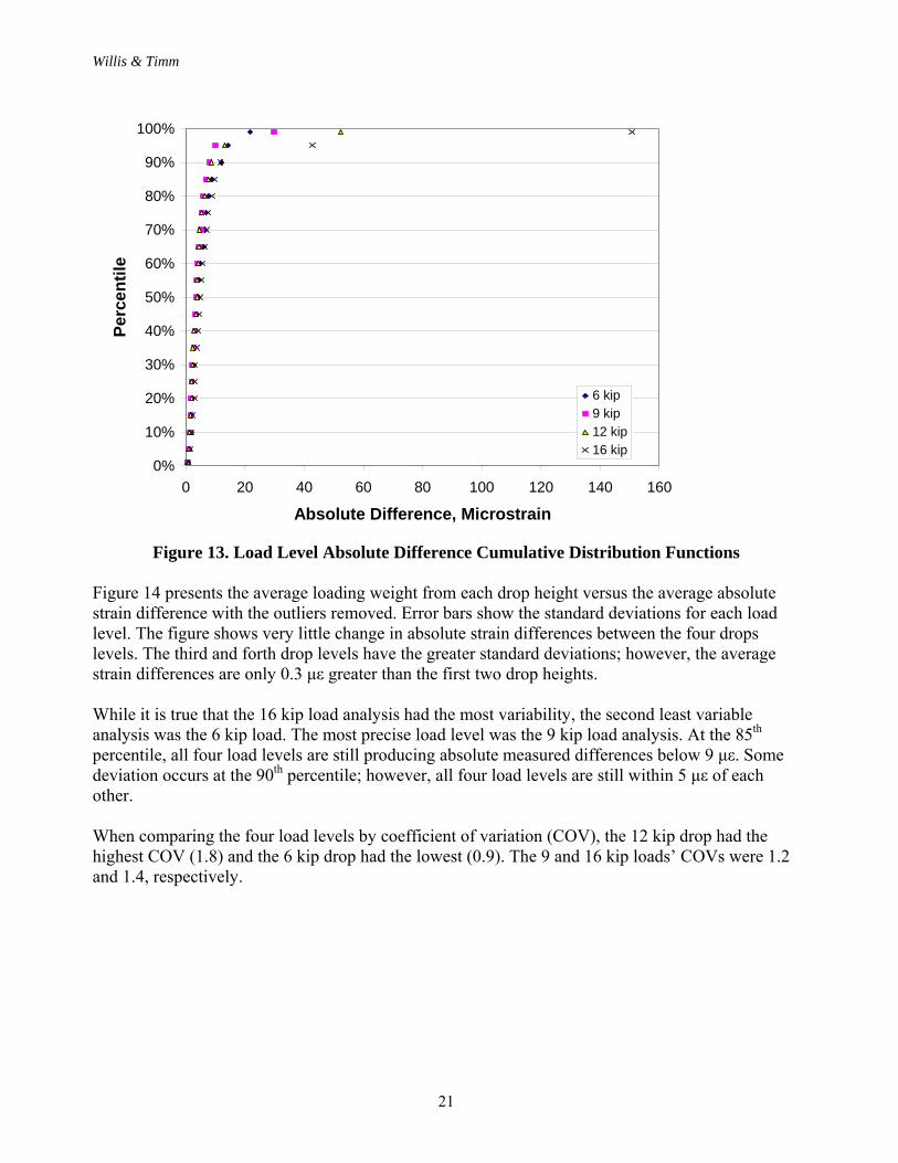
Figure 13 presents the cumulative distribution plots for the four load levels. This plot shows that for the 16 kip loading analysis two datapoints represent extreme outliers (greater than three standard deviations from the average) from the raw dataset having absolute differences greater than 145 microstrains. Removal of these two outliers from the raw dataset shifted the average down and greatly reduced the standard deviation of the 16 kip grouping. An ANOVA test ( = 0.05) was conducted on the four datasets before and after the two outliers had been removed. When these two outliers were included in the data, the p-value was 0.0361; however, their removal changed the ANOVA p-value to 0.396.
0
100
200
300
400
500
600
700
800
900
1000
0 2000 4000 6000 8000 10000 12000 14000 16000 18000
Force, lbs
Mic
rost
rain
Figure 12. Strain Level versus Force - All Sections
Willis & Timm
21
0%
10%
20%
30%
40%
50%
60%
70%
80%
90%
100%
0 20 40 60 80 100 120 140 160
Absolute Difference, Microstrain
Per
cen
tile
6 kip9 kip12 kip16 kip
Figure 13. Load Level Absolute Difference Cumulative Distribution Functions
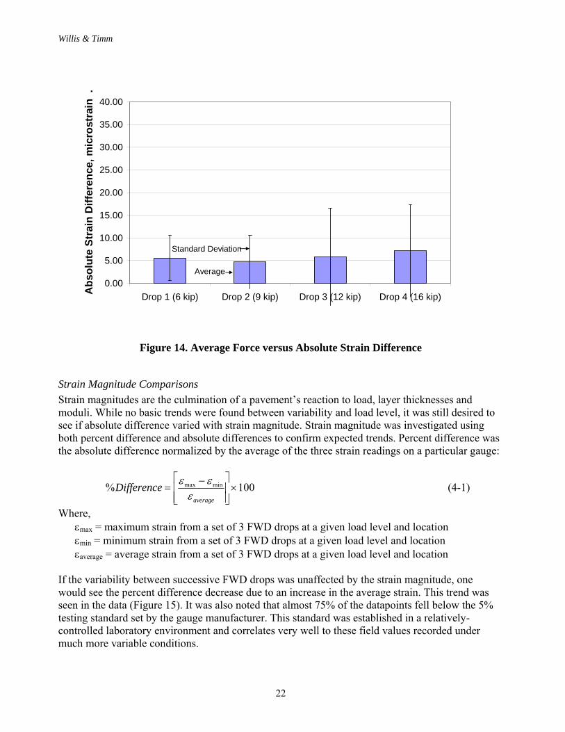
Figure 14 presents the average loading weight from each drop height versus the average absolute strain difference with the outliers removed. Error bars show the standard deviations for each load level. The figure shows very little change in absolute strain differences between the four drops levels. The third and forth drop levels have the greater standard deviations; however, the average strain differences are only 0.3 με greater than the first two drop heights. While it is true that the 16 kip load analysis had the most variability, the second least variable analysis was the 6 kip load. The most precise load level was the 9 kip load analysis. At the 85th percentile, all four load levels are still producing absolute measured differences below 9 με. Some deviation occurs at the 90th percentile; however, all four load levels are still within 5 με of each other. When comparing the four load levels by coefficient of variation (COV), the 12 kip drop had the highest COV (1.8) and the 6 kip drop had the lowest (0.9). The 9 and 16 kip loads’ COVs were 1.2 and 1.4, respectively.
Willis & Timm
22
0.00
5.00
10.00
15.00
20.00
25.00
30.00
35.00
40.00
Drop 1 (6 kip) Drop 2 (9 kip) Drop 3 (12 kip) Drop 4 (16 kip)
Ab
solu
te S
trai
n D
iffe
ren
ce,
mic
rost
rain
.
Average
Standard Deviation
Figure 14. Average Force versus Absolute Strain Difference
Strain Magnitude Comparisons
Strain magnitudes are the culmination of a pavement’s reaction to load, layer thicknesses and moduli. While no basic trends were found between variability and load level, it was still desired to see if absolute difference varied with strain magnitude. Strain magnitude was investigated using both percent difference and absolute differences to confirm expected trends. Percent difference was the absolute difference normalized by the average of the three strain readings on a particular gauge:
100% minmax
average
Difference
(4-1)
Where, max = maximum strain from a set of 3 FWD drops at a given load level and location min = minimum strain from a set of 3 FWD drops at a given load level and location average = average strain from a set of 3 FWD drops at a given load level and location
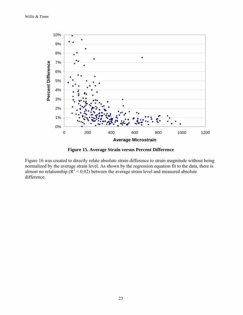
If the variability between successive FWD drops was unaffected by the strain magnitude, one would see the percent difference decrease due to an increase in the average strain. This trend was seen in the data (Figure 15). It was also noted that almost 75% of the datapoints fell below the 5% testing standard set by the gauge manufacturer. This standard was established in a relatively-controlled laboratory environment and correlates very well to these field values recorded under much more variable conditions.
Willis & Timm
23
0%
1%
2%
3%
4%
5%
6%
7%
8%
9%
10%
0 200 400 600 800 1000 1200
Average Microstrain
Per
cen
t D
iffe
ren
ce
Figure 15. Average Strain versus Percent Difference
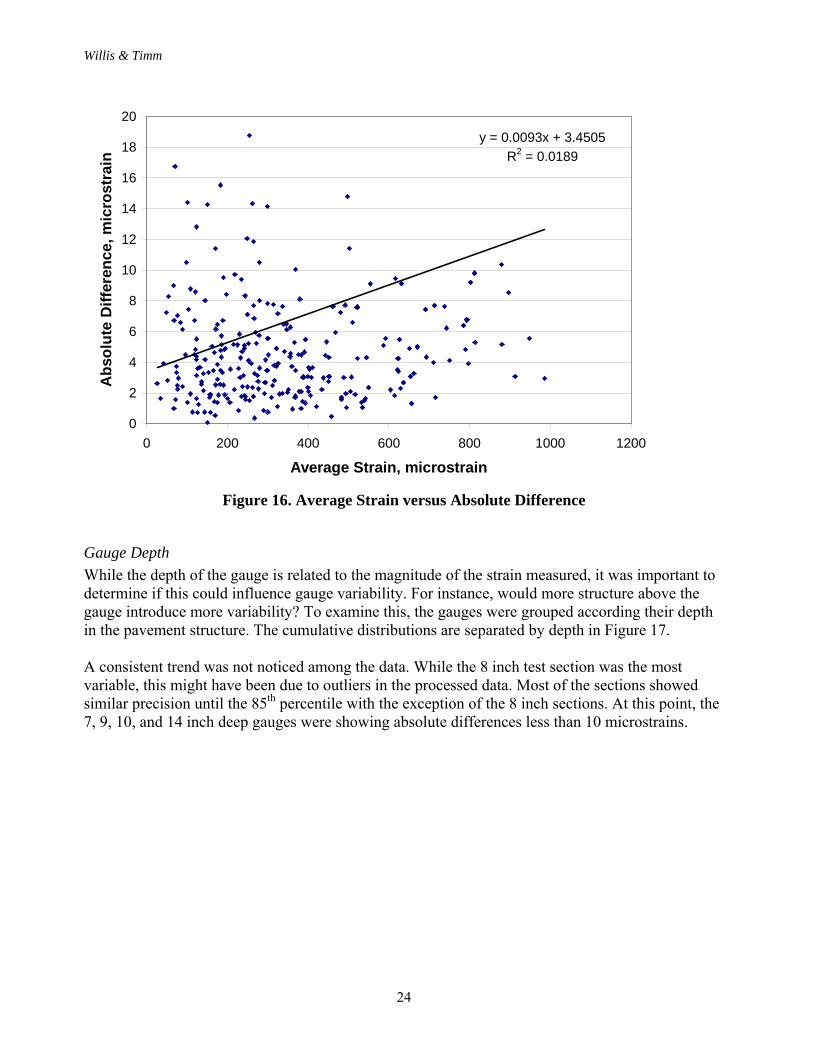
Figure 16 was created to directly relate absolute strain difference to strain magnitude without being normalized by the average strain level. As shown by the regression equation fit to the data, there is almost no relationship (R2 < 0.02) between the average strain level and measured absolute difference.
Willis & Timm
24
y = 0.0093x + 3.4505
R2 = 0.0189
0
2
4
6
8
10
12
14
16
18
20
0 200 400 600 800 1000 1200
Average Strain, microstrain
Ab
solu
te D
iffe
ren
ce, m
icro
stra
in
Figure 16. Average Strain versus Absolute Difference
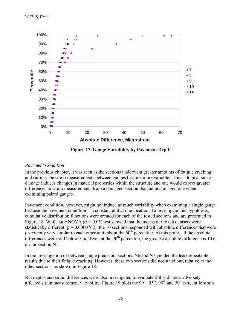
Gauge Depth
While the depth of the gauge is related to the magnitude of the strain measured, it was important to determine if this could influence gauge variability. For instance, would more structure above the gauge introduce more variability? To examine this, the gauges were grouped according their depth in the pavement structure. The cumulative distributions are separated by depth in Figure 17. A consistent trend was not noticed among the data. While the 8 inch test section was the most variable, this might have been due to outliers in the processed data. Most of the sections showed similar precision until the 85th percentile with the exception of the 8 inch sections. At this point, the 7, 9, 10, and 14 inch deep gauges were showing absolute differences less than 10 microstrains.
Willis & Timm
25
0%
10%
20%
30%
40%
50%
60%
70%
80%
90%
100%
0 10 20 30 40 50 60 70
Absolute Difference, Microstrain
Per
cen
tile 7
891014
Figure 17. Gauge Variability by Pavement Depth
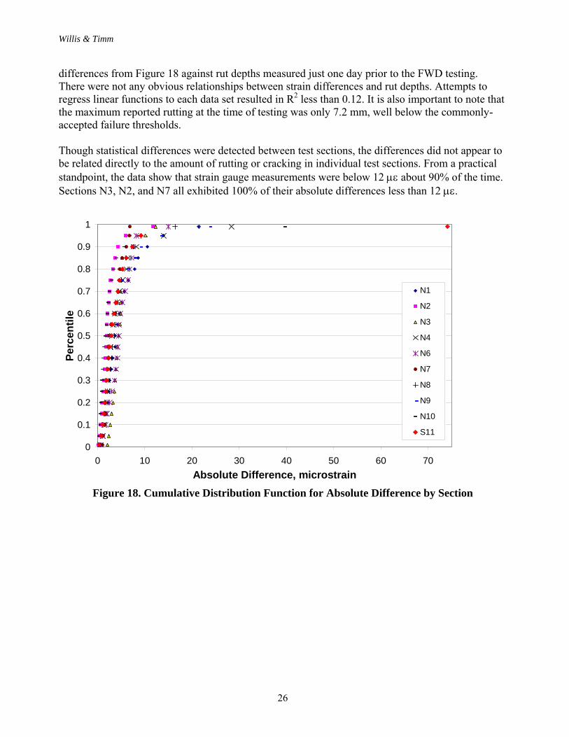
Pavement Condition
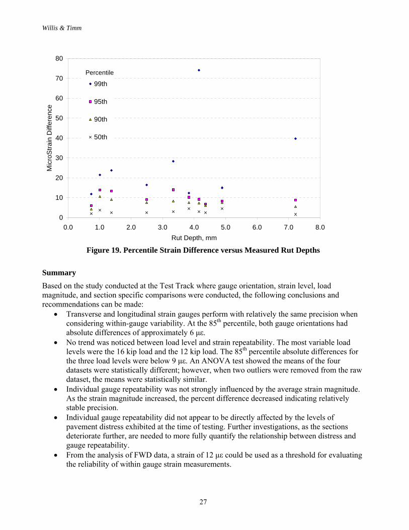
In the previous chapter, it was seen as the sections underwent greater amounts of fatigue cracking and rutting, the strain measurements between gauges became more variable. This is logical since damage induces changes in material properties within the structure and one would expect greater differences in strain measurements from a damaged section than an undamaged one when examining paired gauges. Pavement condition, however, might not induce as much variability when examining a single gauge because the pavement condition is a constant at that one location. To investigate this hypothesis, cumulative distribution functions were created for each of the tested sections and are presented in Figure 18. While an ANOVA ( = 0.05) test showed that the means of the ten datasets were statistically different (p = 0.0000762), the 10 sections responded with absolute differences that were practically very similar to each other until about the 60th percentile. At this point, all the absolute differences were still below 5 . Even at the 90th percentile, the greatest absolute difference is 10.6 for section N1. In the investigation of between gauge precision, sections N6 and N7 yielded the least repeatable results due to their fatigue cracking. However, these two sections did not stand out, relative to the other sections, as shown in Figure 18. Rut depths and strain differences were also investigated to evaluate if this distress adversely affected strain measurement variability. Figure 19 plots the 99th, 95th, 90th and 50th percentile strain
Willis & Timm
26
differences from Figure 18 against rut depths measured just one day prior to the FWD testing. There were not any obvious relationships between strain differences and rut depths. Attempts to regress linear functions to each data set resulted in R2 less than 0.12. It is also important to note that the maximum reported rutting at the time of testing was only 7.2 mm, well below the commonly-accepted failure thresholds. Though statistical differences were detected between test sections, the differences did not appear to be related directly to the amount of rutting or cracking in individual test sections. From a practical standpoint, the data show that strain gauge measurements were below 12 about 90% of the time. Sections N3, N2, and N7 all exhibited 100% of their absolute differences less than 12 .
0
0.1
0.2
0.3
0.4
0.5
0.6
0.7
0.8
0.9
1
0 10 20 30 40 50 60 70
Absolute Difference, microstrain
Per
cen
tile
N1
N2
N3
N4
N6
N7
N8
N9
N10
S11
Figure 18. Cumulative Distribution Function for Absolute Difference by Section
Willis & Timm
27
0
10
20
30
40
50
60
70
80
0.0 1.0 2.0 3.0 4.0 5.0 6.0 7.0 8.0
Rut Depth, mm
Mic
roS
tra
in D
iffer
ence
99th
95th
90th
50th
Percentile
Figure 19. Percentile Strain Difference versus Measured Rut Depths
Summary
Based on the study conducted at the Test Track where gauge orientation, strain level, load magnitude, and section specific comparisons were conducted, the following conclusions and recommendations can be made:
Transverse and longitudinal strain gauges perform with relatively the same precision when considering within-gauge variability. At the 85th percentile, both gauge orientations had absolute differences of approximately 6 με.
No trend was noticed between load level and strain repeatability. The most variable load levels were the 16 kip load and the 12 kip load. The 85th percentile absolute differences for the three load levels were below 9 με. An ANOVA test showed the means of the four datasets were statistically different; however, when two outliers were removed from the raw dataset, the means were statistically similar.
Individual gauge repeatability was not strongly influenced by the average strain magnitude. As the strain magnitude increased, the percent difference decreased indicating relatively stable precision.
Individual gauge repeatability did not appear to be directly affected by the levels of pavement distress exhibited at the time of testing. Further investigations, as the sections deteriorate further, are needed to more fully quantify the relationship between distress and gauge repeatability.
From the analysis of FWD data, a strain of 12 με could be used as a threshold for evaluating the reliability of within gauge strain measurements.
Willis & Timm
28
CHAPTER 5 – CONCLUSIONS AND RECOMMENDATIONS Embedded strain gauges are being more commonly used at accelerated loading facilities as a way to quantify the mechanistic responses occurring during pavement loading. These measured responses are helping bridge the gap between the mechanistic and empirical portions of M-E design. For this purpose, it is important to identify a suitable technique for evaluating the reliability of strain measurements.
Conclusions
Based on the study where both between and within gauge variability were analyzed, the following conclusions can be drawn:
Longitudinal gauges had slightly more consistent readings than the transverse gauges between gauges. This was explained through theoretical modeling where transverse strain was affected slightly more by wheel placement.
Steer axles caused less measured absolute differences between gauges than tandem and singles axles.
Cracked sections displayed more erratic and less repeatable strain measurements between gauges.
Sections free from cracking showed 80% of their absolute measured differences to be below 30 με between gauges.
Transverse and longitudinal strain gauges perform with relatively the same precision for within-gauge precision. At the 85th percentile, both gauge orientations had absolute strain differences of approximately 6 με.
No trend was noticed between load level and strain repeatability. Once outliers from the most variable dataset had been removed, an ANOVA analysis showed the means were not statistically different.
Individual gauge repeatability was not strongly influenced by the average strain magnitude. As the strain magnitude increased, the percent difference decreased indicating relatively constant repeatability.
Individual gauge repeatability did not appear to be directly affected by the levels of pavement distress exhibited at the time of testing. Further investigations, as sections deteriorate further, are needed to more fully quantify the relationship between distress and within-gauge repeatability.
Test sections exhibited 90% of the measured absolute differences within gauges below 12 με.
Recommendations
To validate instrumentation in the field, the following recommendations are made: Testing should be conducted early after instrumentation has been installed to prevent
cracking from influencing gauge measurements. More testing should be conducted to determine an appropriate working range for strain
gauge variability at different accelerated loading facilities. A benchmark of 30 με will be used for between gauge variability at the Test Track. This
benchmark should be used during the data screening process. If paired gauges are showing
Willis & Timm
29
deviations beyond 30 με, careful examinations should occur as to why. This might include testing individual gauges for repeatability using the FWD testing procedure.
A benchmark of 12 με will be used as a new benchmark for within gauge variability. During future testing cycles, FWD on-gauge testing will be conducted before trafficking occurs to ensure the gauges are working properly. The absolute differences for a gauge should be below this benchmark.
While FWD testing is more repeatable and more reproducible than truck trafficking, previous research conducted at the Test Track indicates that these gauges should behave similarly under live truck traffic, though more variability is observed under live trafficking.
Strain gauges incorporated in the validation process of M-E design should undergo variability analysis along with calibration. If the gauges are proven to be reliable, more confidence will be instilled in the models developed by data collected from these gauges.
Willis & Timm
30
REFERENCES
1. Monismith, C.L. Analytically Based Asphalt Pavement Design and Rehabilitation: Theory in Practice, 1962-1992. Transportation Research Record: Journal of the Transportation Research Board, No. 1354, TRB, National Research Council, Washington, D.C., 1992, pp. 5-26.
2. Kentucky Transportation Cabinet. Pavement Design Guide (2007 Revision) for Projects off the National Highway System less than 20,000,000 ESALs, less than 15,000 AADT, and less than 20% trucks. Kentucky Transportation Cabinet Division of Highway Design, Lexington, KY, 2007.
3. Timm, D.H., D. E. Newcomb, and B. Birgisson. Development of Mechanistic-Empirical Design for Minnesota. Transportation Research Record: Journal of the Transportation Research Board, No. 1629, TRB, National Research Council, Washington, D.C., 1998, pp.181-188.
4. Thickness Design, Asphalt Pavements for Highways and Streets. Report MS-1, The Asphalt Institute, 1982.
5. Timm, D.H. and A.L. Priest. Material Properties of the 2003 NCAT Test Track Structural Study. Report No 06-01, National Center for Asphalt Technology, Auburn University, 2006.
6. Miner, M.A. Estimation of Fatigue Life with Emphasis on Cumulative Damage. Metal Fatigue, edited by Sines and Wiseman, McGraw Hill, 1959, pp 278-89.
7. Al-Qadi, I., A Loulizi, M. Elseifi, and S. Lahouar. The Virginia Smart Road: The Impact of Pavement Instrumentation on Understanding Pavement Performance. Journal of the Association of Asphalt Paving Technologists, Vol. 73, 2004, pp. 427-466.
8. Siddharthan, R.V., P.E. Sebaaly, M. El-Desouky, D. Strand, and D. Huft. Heavy Off-Road Vehicle Tire-Pavement Interactions and Response. Journal of Transportation Engineering, Vol. 131, 2005, pp. 239-247.
9. Howard, I.L., K.A. Warren, C. Eamon, and C. R. Lord. Variability Analysis of Thin Instrumented Flexible Pavements. Submitted to the 87th Annual Meeting of the Transportation Research Board, Washington, D.C., 2008.
10. Romanoschi, S.A., A. Gisi, M. Portillo, and C. Dumitru. “The first findings from the Kansas Perpetual pavement experiment.” 87th Annual Meeting of the Transportation Research Board, Washington, D.C., 2008 (CD-ROM).
11. Timm, D.H., A.L. Priest and T.V. McEwen. Design and Instrumentation of the Structural Pavement Experiment at the NCAT Test Track. Report No. 04-01, National Center for Asphalt Technology, Auburn University, 2004.
Willis & Timm
31
12. Timm, D.H. Design, Construction and Instrumentation of the 2006 Test Track Structural Study. Draft Report, National Center for Asphalt Technology, Auburn University, 2008.
13. Timm, D.H. and A.L. Priest. Wheel Wander at the NCAT Test Track. Report No 05-02, National Center for Asphalt Technology, Auburn University, 2005.
14. Willis, J.R. Field-Based Strain Thresholds for Flexible Perpetual Pavement Design. Doctoral Dissertation, Auburn University, 2009.
15. Saint John’s University. Kolmogorov-Smirnov Test. College of Saint Benedicts and Saint John’s University. www.physics.csbsju.edu/stats/KS-test.html. Accessed July 18, 2008.