Renormalization of Random Jacobi Operatorsknill/offprints/renormalization.pdf · Renormalization of Random Jacobi Operators 197 J of the quadratic map z ι-» z2 + E. Moreover, we

Commun. Math. Phys. 164, 195-215 (1993) Communications ΪΠ

MathematicalPhysics

© Springer-Verlag 1994

Renormalization of Random Jacobi Operators

Oliver Knill*

Mathematikdepartment, ETH Zurich, CH-8092 Zurich, Switzerland

Received August 13, 1993/in revised form December 3, 1993

Abstract: We construct a Cantor set ̂ of limit-periodic Jacobi operators having thespectrum on the Julia set J of the quadratic map z ι-> z2 + E for large negative realnumbers E. The density of states of each of these operators is equal to the uniqueequilibrium measure μ on J. The Jacobi operators in $ are defined over the vonNeumann-Kakutani system, a group translation on the compact topological group ofdyadic integers. The Cantor set $ is an attractor of the iterated function system builtup by the two renormalisation maps Φ± : L = ψ(D2

L + E) ι-> D±. To prove thecontraction property, we use an explicit interpolation of the Backlund transformationsby Toda flows. We show that the attractor $ is identical to the hull of the fixed point

1. Introduction

Random Jacobi operators are discrete one-dimensional Laplacians and are discreteapproximations of one-dimensional random Schrodinger operators. The literatureabout such operators is huge and a part is by now covered by text books like [CFKS,CL, C, PF].

Dynamical systems obtained by iteration of rational maps have a rich structure.Among these systems, the quadratic map z ι—> z2 + E is studied best. For reviews inthe large literature we refer to [Bla, CG, Ere, M].

Toda differential equations are integrable Hamiltonian systems and are discretisa-tions of the Korteweg de Vries systems. According to the chosen boundary condition,the investigation of the Toda systems touches different areas in mathematics. We referto [FT, Tod, Per, Kl].

The subject of this article is located in the intersection of the above three fields.We study random Jacobi operators having the symmetry of being invariant under a

Present address: Department of Mathematics, Caltech, Pasadena, CA 91125, USA

196 O. Knill

scale transformation given by a doubling of the lattice spacing, a squaring of theoperator and an adaptation of the energy:

<F : D h-> ψ(D2 + E) ,

where ψ is the restriction of the Laplacian to the coarser lattice. More precisely,assuming that D is an off-diagonal disorder Jacobi matrix (Du)n = dnun+l +

dn_ι^n_ι, the matrix L = D2 + E is given by Lun = anun+2 + an_2un_2 + bnun,

with an = dndn+l and bn = E + d2

n + d2

n_λ. This operator is the direct sum of

two Jacobi matrices. One of them is Lnπι = [ψ(D2 + E)] nπι = [D2 + E] 2rlj2m.

Because L has also diagonal entries, the map ̂ can not be iterated. However, wehave shown in [K2] that the inverse of ̂ can always be computed in the class ofrandom Jacobi operators: given L, there exist two new Jacobi operators D± definedover a new renormalized dynamical system such that ^(D±) = L. The entries ofD± are constructed from the Titchmarsh-Weyl functions of L. The aim of this workis to study the iteration of the maps

Φ± : L = ψ(D2

± + E) ̂ D± .

These maps on operators correspond on the spectral level to the two inverses 0± of

the quadratic map z H- » z2 + E. Here is the link between random Jacobi operatorsand the iteration of the quadratic map.

Before we outline the content of our results, we mention the earlier works ofBaker, Barnsley, Bellissard, Bessis, Geronimo, Harrington, Mehta and Moussa, whoconstructed semi-infinite Jacobi operators L E J?(/2(N)) with spectra on Julia setsJ (see [Bak, BBM, BGM, BMM, BGH2, BGH3]). Such operators have also theequilibrium measure on the Julia set as the density of states and satisfy the fixedpoint equation ψ(L2 + E) = L. The side diagonal dn = [L] +l of L begins with

d0 = [L]01 = 0, ̂ = [L]12 = VE,d2 = [L]23 = 1, . . . ,

where the entries dk are obtained recursively using d2

2n+l = -d\n — E, d2

n -

d2nd2n_l. Our set up is different in that we construct Jacobi matrices by renor-

malisation maps Φ± which can only be defined in J?(/2(Z)) and not in ^(/2(N)),whereas the fixed point equation of the renormalisation equation has a solution alsoin «J?(72(N)). For the construction of the attractor, we have to work in an algebra ofrandom operators rather then in J?(72(Z)).

The set of random Jacobi operators forms a fiber bundle over the topological group% of dynamical systems: over each dynamical system is defined the Banach spaceof random Jacobi operators which is a subspace of the crossed product of L°°(X)with the dynamical system. The factorization result in [K2] can be restated in sayingthat the 2 : 1 integral extension map Φ on %6 can be lifted to two renormalizationmaps Φ± defined on an open set of the bundle. A pair (T, L), where L is a Jacobioperator over the dynamical system (X, T, m) is mapped into a pair (5, £>±), where

ip(D2

± + E) = L and S is an integral extension of T satisfying S2 = T. We willshow that for large enough real — E, both renormalization maps Φ± are contractionson an open set of the bundle forming a so called hyperbolic iterated function systemhaving an attractor β> which is a Cantor set in the fiber 2> over the von NeumannKakutani system.

The spectrum of L = ψ(D2 + E) and the spectrum of D are related byσ(D)2 + E = σ(L) and the spectrum of each operator L G $ is the Julia set

Renormalization of Random Jacobi Operators 197

J of the quadratic map z ι-» z2 + E. Moreover, we will show that the density ofstates of L is the unique equilibrium measure on J. The Lyapunov exponent turnsout to be the potential theoretical Green function of the Julia set and the determinantz H^ det(L — z) of an operator L E $> is the Boucher function which conjugates themap z i—> z2 + E to z »—> z2 in a neighborhood of oc.

The factorization L = ?/;(D2 + E) is the key for isospectral Backlund transforma-tions, translations by one unit on the finer lattice. A main tool to prove our resultsis the following interpolation of Backlund transformations BT± by a Toda flow with

a time-dependent Hamiltonian HE(L) = ±tr(hE(L)) = ̂ ^w(E\ where w(E) is theFloquet exponent of L. The interpolating Toda flow is

1 \ + / 1

L-EJ \L-E

It follows from this Toda interpolation that BT±(L) is unitarily equivalent to L. Itis here, where the theory of integrable systems enters. We mention, that for the KdVequation, there exists a similar interpolation of the Backlund transformation given bya time-dependent KdV flow

dE

where GXX(E, L) = (L — E)~x is the Green function of the Schrδdinger operatorL = -D2 + q. (See [McK] p. 31.)

The hull & of the fixed point L+ of Φ+ is the set of all translates of L+(TX),where Tx is the translation belonging to any element x in the group X of dyadicintegers. Every L E $ belongs to some ω £ Ω = {—1,1}N by

L = Φ(ώ) = lim Φω Φω ... Φω K .Tl—*OO 1 2 il

A change of alphabet 1 ι-» 0, — l,ι-» 1 identifies an element ω £ Ω = { — l,l}N

with an element x(ώ) E X = {0,1}N. We will prove that Φ(ώ) = I/+(Tx(ω)), whichimplies @ - ̂ and means that each element of the attractor of the iterated functionsystem is obtained by an explicitly known translation of the fixed point L+.

2. The von Neumann Kakutani System

The set % of automorphisms of a Lebesgue space (X, ra) is a complete topologicalgroup when equipped with the uniform topology given by the metric d(T, 5) = m{x EX I T(x) 1 S(x)}. For T G ̂ , we call (X, Γ, m) a dynamical system.

Given a function / G Ll(X,J$ \ {0}), a new dynamical system (X? ,T? , m f )called the integral extension is defined as follows (see [CFS]). Define X^ :={ ( x , ϊ ) \ x £ X and 1 < i < f ( x ) } and a probability measure τ?τ/ on Xf by

, i)) = m(Y)/ f f dm. This measure is preserved by the transformation

ί (^^ + 1) , if i + 1 <) , if z + l =

This construction gives also a map Φ ̂ : % — > ̂ because the integral transformationis again an automorphism of (X, m) after an identification of the Lebesgue spaces

198 O. Knill

Proposition 2.1. For f f dm ^ 1, the map Φ$ is a contraction on % and has a

unique fixed point T? .

Proof. The contraction property follows because for all T^T^ £ %

m{{Tλ(x) i T2(x)}) = ( ί fdπλ m({Γ,(x) J T2(x)}) .\J /

Apply Banach's fixed point theorem in the complete metric space .̂ D

We consider now the special case of an integral extension with / = 2, where theidentification of X = [0, 1] with X? is given by

X = [0, 1] -» (X, {!}) U (X, {2}) = Xf = [0, 1/2] U [1/2, 1] .

In order to fix the ideas we can write a dynamical system as a measurable mapT : [0, 1] — » [0, 1] leaving invariant the Lebesgue measure on [0, 1] and define φf by

x + 1 / 2 , if *e *!=[(>, 1/2),

The unique fixed point T of Φ = φf , with /(#) = 2 is called the von Neumann-Kakutani system. It is by construction a piecewise translation of intervals

T(x) = x+I-Cn+l, for Cn < x < Cn+l ,

n

where C0 = 0 and Cn = ̂ 2~x, n > 0 . The system (X, Γ, m) is ergodic and has adiscrete spectrum ί=l

(see [P, F]). T is conjugated to a group translation on the compact abelian group Gof dyadic integers, the dual group of G C T1. The group G is the space of sequencesω = {α j , C J 2 , . •} in {0,1}N with group operation

(ω + η)n = ωn + ηn + pn_l (mod 2) ,

where p0 = 0 and pn G {0,1} is equal to 1 if and only if ωn + ηn + ρn_λ > 2. Theoo

group translation Tλ : ω H-> ω + (1,0,0,...) is conjugated by ω »-» Σ ωn^~n ^ $> Ήto the map T on the interval /. n=1

3. Random Jacobi Operators

The crossed product JΓ of L°°(JΓ, C) with the dynamical system (X, T, m) is a C*algebra consisting of operators K - Σ Knr

n with convolution multiplication

(KkMm(Tk))τn

n k+m=n

and norm |||^||| - | ||ΛΓ(x)|| 1^, where K(x) is the infinite matrix

[K(x)]mn = Kn_m(Tmx) .


The adjoint of an operator is defined by requiring r* = τ~l. A trace on JΓ is givenby tτ(K) = / K0 dm. A random Jacobi operator L is an element in & of the form

x

L = aτ + a(T~l)τ* + b

with α, b e I/°°(.X, C). We denote by S C JΓ the complex Banach space of randomJacobi operators. We call M(L) := exp ( Jlog |α| dm) the mass of a Jacobi operator.If log |α > <5 > 0 for some <5 > 0, we say, the operator has a positive definite mass.Notice that random Jacobi operators are only normal, if α, b are real. Denote by Φ(JΓ)the C* -algebra corresponding to the renormalized system (X, Φ(T),m). As long aswe consider only one renormalization step, we denote the renormalized dynamicalsystem with (Y, S, n) and the von Neumann algebra with ̂ and elements in ̂ byB - ΣBnσ

n, where σ is the symbol in ̂ corresponding to r in JΓ. Call ψ the

map jμ

where Kn(x) - K2n(x) for x € Xt = X. The mapping ^ gives for almost all x G

Let L € o^ be a random Jacobi operator having positive mass. For E outside aball containing the spectrum of I/, the Titchmarsh-Weyl functions are given by

u±(Tx)±m±(x) = a(x) - — - , n±(x) = α(T±- — - , ± = - — — ,u±(x) ± u±(x)

where ^±(x) e Rz are solutions of L(x) = Eu(x) with X] \(u±)n(x)\2 < oo. These±n>0

functions are measurable according to the multiplicative ergodic theorem of Oseledecand are bounded. Using Lu± = au±(T) + a(T~l)u±(T~l) + bu± = Eu± and thedefinition of ra±, n±, we get

m± + n± = E — b ,

m± ' n±(Ώ - β2

New random Jacobi operators

D± = y^σ + yJc±(S-l)σ* € $ί

are obtained with functions c± € L°°(y, C) defined by requiring that for x G X = Xl9

c±(x) = -m±(x), c±(S~lx) = -n±(x) .

The sign of D± is specified if we take the principal branch of the square root for/— m± and the branch -V— n± such that α = <\/m±n±(T). We get then

c±(c±(S~lx) = -E + b(x) ,

c±(x) c±(Sx) = a2(x) .

As c is defined on Y, these formulas extend the functions α, 6 G L°°(X, C) to functions

200 O. Knill

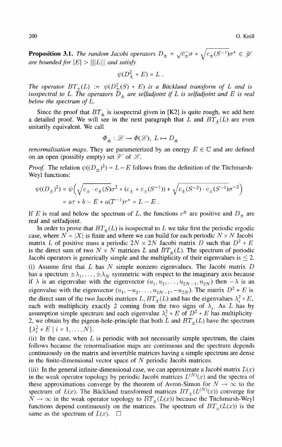
Proposition 3.1. The random Jacobi operators D± =are bounded for \E\ > \\\L\\\ and satisfy

ψ(D2

± +E) = L.

The operator BT_±(L) := ψ(D^_(S) + E) is a Bάcklund transform of L and isίsospectral to L. The operators D± are selfadjoint if L is selfadjoint and E is realbelow the spectrum of L.

Since the proof that BT± is isospectral given in [K2] is quite rough, we add herea detailed proof. We will see in the next paragraph that L and BT±(L) are evenunitarily equivalent. We call

Φ± : S§ -> ΦC5ί), L h-> D±

renormalisation maps. They are parameterized by an energy E E C and are definedon an open (possibly empty) set ̂ of =3ί.

Proof. The relation ψ((D±)2) - L — E follows from the definition of the Titchmarsh-Weyl functions:

c±(S)σ2 + (c± + c±(S'1))

= aτ + b-E + a(T~l)τ* = L-E .

If E is real and below the spectrum of L, the functions c^ are positive and D± arereal and selfadjoint.

In order to prove that BT±(L) is isospectral to L we take first the periodic ergodiccase, where N = \X\ is finite and where we can build for each periodic TV x N Jacobimatrix L of positive mass a periodic 2N x 2N Jacobi matrix D such that D2 + Eis the direct sum of two N x N matrices L and BT±(L). The spectrum of periodicJacobi operators is generically simple and the multiplicity of their eigenvalues is < 2.

(i) Assume first that L has N simple nonzero eigenvalues. The Jacobi matrix Dhas a spectrum ±λ 1 ? . . . , iλ^y symmetric with respect to the imaginary axis becauseif λ is an eigenvalue with the eigenvector (w l 5 u2, - ,u2N_ι,u2N) then — λ is an

eigenvalue with the eigenvector (ul7 —u2,.. - , ^2W-ι> ~U2N^ ^ne matriχ D2 + E isthe direct sum of the two Jacobi matrices L, BT±(L) and has the eigenvalues λ^ + E,each with multiplicity exactly 2 coming from the two signs of \. As L has byassumption simple spectrum and each eigenvalue X2 + E of D2 + E has multiplicity2, we obtain by the pigeon-hole-principle that both L and BT±(L) have the spectrum

{X2

i+E\i = l,...,N}.

(ii) In the case, when L is periodic with not necessarily simple spectrum, the claimfollows because the renormalisation maps are continuous and the spectrum dependscontinuously on the matrix and invertible matrices having a simple spectrum are densein the finite-dimensional vector space of N periodic Jacobi matrices.

(iii) In the general infinite-dimensional case, we can approximate a Jacobi matrix L(x)in the weak operator topology by periodic Jacobi matrices L^N\x) and the spectra ofthese approximations converge by the theorem of Avron-Simon for TV —> oo to thespectrum of L(x). The Backlund transformed matrices BT±(L(N\x)) converge forN —> oo in the weak operator topology to BT±(L(x}) because the Titchmarsh-Weylfunctions depend continuously on the matrices. The spectrum of BT±(L(x)) is thesame as the spectrum of L(x). HI


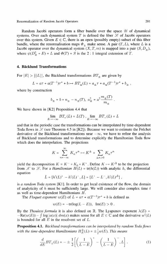
Random Jacobi operators form a fiber bundle over the space ί& of dynamicalsystems. Over each dynamical system T is defined the fiber S§ of Jacobi operatorsover this system. Given E £ C, there is an open (possibly empty) subset of this fiberbundle, where the renormalisation maps Φ± make sense. A pair (Γ, L), where L is aJacobi operator over the dynamical system (X, T, ra) is mapped into a pair (5, D±\

where V>(£>± + E) = L and Φ(Γ) = 5 is the 2 : 1 integral extension of T.

4. Backlund Transformations

For [E1 1 > I H Z / H I , the Backhand transformations BT± are given by

±L - ar + a(T~l)τ* + b^ BT±(L) = a±r + a±(T~l)τ* + b

where by construction

2 — -b± - b + n± - n±(T), a2

± - a2

ΉΊ-j_

We have shown in [K2] Proposition 4.4 that

lim BT+ (L) = L(T) , lim BT_(L) = LE^-oo E-+-OO

and that in the periodic case the transformations can be interpolated by time-dependentToda flows in ̂ (see Theorem 4.5 in [K2]). Because we want to estimate the Frechetderivative of the Backlund transformations near — oo, we have to refine the analysisof Backlund transformations and to determine explicitly the Hamiltonian Toda flowwhich does the interpolation. The projections

oo

K = E κ^n ~ κ± = Σ κ^n

n= — oo ±n>0

yield the decomposition K - K~ + KQ + K+ . Define K *— > KΔ to be the projectionfrom JΓ to 3$. For a Hamiltonian H(L) = tr(/ι(L)) with analytic ft, the differentialequation

L = (ti(L)+ - h'(LΓ,L] = [L+ - L-,h'(L)Δ] ,

is a random Toda system [Kl]. In order to get local existence of the flow, the domainof analyticity of ft must be sufficiently large. We will consider also complex time tas well as time-dependent Hamiltonians H.

The Floquet exponent w(E) of L = αr + α(T-1)r* + b is defined as

w(E) = -tr(log(L - E)), Im(£) > 0 .

By the Thouless formula it is also defined on R. The Lyapunov exponent λ(E) -—Re(w(E)) - / log \a(x)\ dm(x) makes sense for all E e C and the derivative w'(L)is bounded for all E in the resolvent set of L.

Proposition 4.1. Backlund transformations can be interpolated by random Toda flows

with the time-dependent Hamiltonians Hg(L) = ±-w(E). This means

7 771 ^" •"- -t- V"/ -̂ /-» I \ r Tn / \ r 7-1 / 5 -̂ | ' V - * - /α^z/

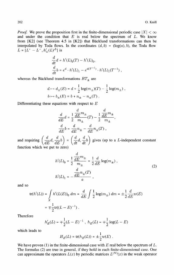
202 O. Knill

Proof. We prove the proposition first in the finite-dimensional periodic case \X\ < ooand under the condition that E is real below the spectrum of L. We knowfrom [K2] (see Theorem 4.5 in [K2]) that Backlund transformations can then beinterpolated by Toda flows. In the coordinates (d, b) = (log(α),6), the Toda flowL = [L+ -L-,h'±(L)Δ] is

7 7 / / f \ /ΓΓJN Z - . ' / 7 ~ \—d = h (L)0(i ) - h (L)0,

whereas the Backlund transformations BT± are

d i—> d±(E) = d+ - log(m±)(T) — - log(m±) ,

b ̂ b±(E) = b + n±- n±(T) .

Differentiating these equations with respect to E

2 m±

v ' 2 m±

and requiring ( — d, -7^^ ) = ( — d, — 6 ) gives (up to a L-independent constantγαj& d-c/ y yαt dt

function which we put to zero)

and so

ti(L(E))0 dm=~ log(m±) dm = ±1 A

x

Therefore

Λ^(i) = T^(£ - E)"1 , hE(L) = T^ logd - E)

which leads to

FB(i) = tr(/ιB(L)) = ±i«;(£0 -

We have proven (1) in the finite-dimensional case with E real below the spectrum of L.The formulas (2) are true in general, if they hold in each finite-dimensional case. Onecan approximate the operators L(x) by periodic matrices L(N\x) in the weak operator


topology. For N -+ oo, we obtain h(L(N>)(x) —> h(L)(x) in the weak operatortopology and (m±)^N\x) —> m±(x) for almost all x G X. (By analytic continuation,the formula (1) holds also for complex numbers E satisfying |£? |> | | |Z/ | | | . ) D

We use this interpolation to estimate the Frechet derivative -jγBT±(L) of theBackhand transformations near oo.

Corollary 4.2. For \E\ —> oo, we havefixed ball B(R) C SS.

dL

1, uniformly for L in each

En-\

Proof. Since there is a uniform bound for the Frechet derivative of

E2 ±BT(L) ^Vfί-^-V -( Ln

dE ^'-^LU-1; ^

on ̂ we have

for \E\ —»• oo. Therefore

oo

where I~ : S —> SZ is the identity operator and Γ (L) = L(T). D

5. Iterated Function Systems

We state now a version of Barnsley's result about hyperbolic iterated function systems[Bar]. Such a result holds in the general context of complete metric spaces. Weformulate and use it in the case when the hyperbolic iterated function system isacting on a Banach space. The proof of the result is given for the convenience of thereader.

Lemma 5.1. Given a Banach space (̂ ,̂ || ||) and two differentiate maps Φ+ , Φ_ :^ C ̂ —> ^/M leaving invariant an open connected bounded subset ^ of Λ&.Assume there exists a common inverse ^ of both Φ+, Φ_ on Φ+ (9^) U ΦSuppose, there exists λ < 1 such that for L G 9^

< λ (3)

and Φ+ (L) ^ Φ_(L)for all L G 9^. Then there exists a Φ± invariant Cantor set

homeomorphic to Ω = {—1,1}N which is the image of the ίnjectίve map

Φ:ω = lim Φ o Φ o ,k—»oo l z

where K e ̂ is arbitrary. The map ̂ restricted to ̂ is topologically conjugatedby Φ to the one-sided Bernoulli shift σ on { — 1,1}N: ̂ o Φ - φ o σ.

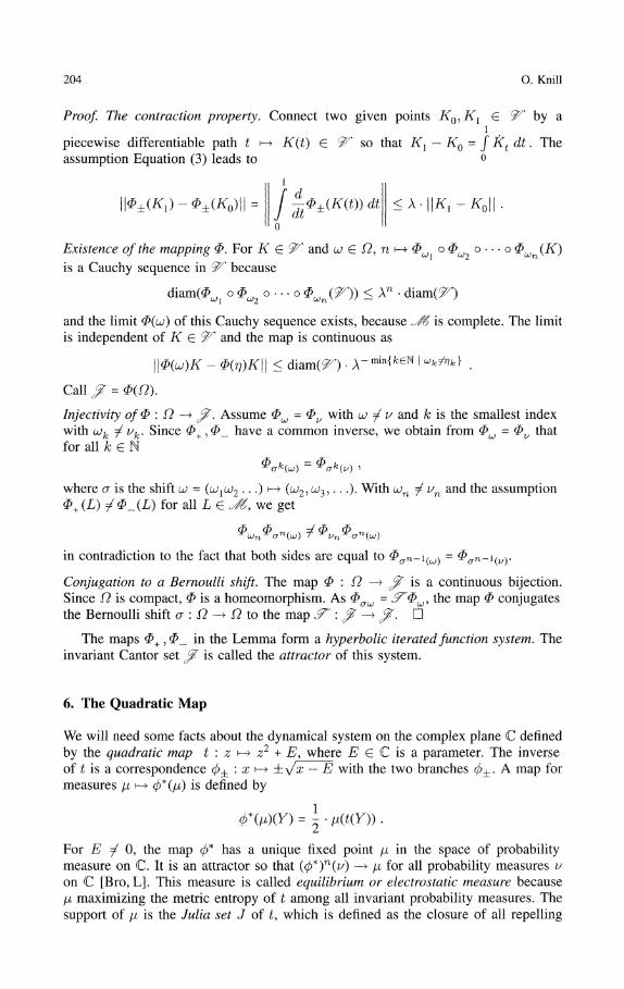
204 O. Knill

Proof. The contraction property. Connect two given points K0,Kl G ^ by a

piecewise differentiable path t ι— >• K(t)assumption Equation (3) leads to

\\Φ±(K])-Φ±(K0)\\ =

so that Kl — K0 = J Kt at . The

dt

Existence of the mapping Φ. For K £ 9^ and ω £ Ω, n *-+ Φω ° Φω o o

is a Cauchy sequence in 9̂ * because

diam(Φω( o Φω2 o < \n diam(^)

and the limit Φ(ω) of this Cauchy sequence exists, because Λ& is complete. The limitis independent of K E 9̂ * and the map is continuous as

\\Φ(ώ)K - Φ(η)K\\ < diam(9O - A~min^eN ' ̂ ^> .

Call ̂ - Φ(Ω}.

Injectivity ofΦ: Ω —> ̂ . Assume Φω - Φv with ω ^ u and k is the smallest indexwith ωk / vk. Since Φ+ , Φ_ have a common inverse, we obtain from Φω = Φv thatfor all k G N

where σ is the shift ω = (ωιω2. .) *—> (^2, cϋ3, . . .). With α;n 7^ z/n and the assumptionΦ+ (L) ^ Φ_(L) for all L G ̂ , we get

in contradiction to the fact that both sides are equal to Φσn~\(ω^ =

Conjugation to a Bernoulli shift. The map Φ : Ω — >Since Ω is compact, Φ is a homeomorphism. As Φσω =the Bernoulli shift σ : Ω -» ί? to the map ̂ : ̂ ->

is a continuous bijection., the map Φ conjugates

D

The maps Φ+ ,Φ_ in the Lemma form a hyperbolic iterated function system. Theinvariant Cantor set ̂ is called the attractor of this system.

6. The Quadratic Map

We will need some facts about the dynamical system on the complex plane C definedby the quadratic map t : z \of t is a correspondence φ± : x ι— »measures μ ι— » φ*(μ) is defined by

+ E, where E G C is a parameter. The inverseX - E with the two branches φ±. A map for

= ' μ(t(Y)) -

For E i 0, the map 0* has a unique fixed point μ in the space of probabilitymeasure on C. It is an attractor so that (0*)n(V) — * μ for all probability measures von C [Bro, L]. This measure is called equilibrium or electrostatic measure becauseμ maximizing the metric entropy of t among all invariant probability measures. Thesupport of μ is the Julia set J of £, which is defined as the closure of all repelling


periodic orbits of t. The measure μ has the property of being balanced [BGH1], whichmeans that for each chosen branch φ±, one has

(μ)(0±00) = \μ(Y)

For large |E|, the two maps φ^ form a hyperbolic iterated function system havingthe Julia set as the attractor. It follows from Barnsley's Lemma 5.1 that t is thentopologically conjugated to a one-sided Bernoulli shift. The Julia set is then calledhyperbolic and is a completely disconnected Cantor set. (See [Bla, C, EL] for reviews.)

7. Existence of the Attractor

We return now to the renormalίsatίon maps Φ± acting on the Banach space J^7

of Jacobi operators defined over the von Neumann Kakutani system (X, T, m). Anelement L = aτ + a(T~l)r* + b E S? is called limit-periodic if for almost all x E Xthe sequences αn = a(Tnx) and bn = b(Tnx) are limit-periodic in the sense that theycan be approximated in /°°(Z) by periodic sequences.

Theorem 7.1. For large enough real —E, the maps Φ+ , Φ_ form a hyperbolic iteratedfunction system defined on an open non-empty set 9^ C 31. Each L E ̂ is limit-periodic and has the spectrum on the Julia set J of the quadratic map t : z ι— > z2 + E.

Proof. Fixing a neighborhood of the Julia set. For large —E, there exists an openφ± -invariant connected real neighborhood V of J that does not contain E.

Fixing an open set of Jacobi operators. The open connected set

9^ = {L E 3§ σ(L) E V, L has positive definite mass }

is not empty: take any L E 3§ with positive definite mass. There exist constantsOL > 0, β E R, such that σ(aL + β) E V.

The renormalisation maps have a common inverse. The inverse of Φ± is given by

^(Ό) = ψ(D2 + E) .

The two renormalίsatίon maps have no common image. For large enough |EΊ and

because Φ+(L) = Φ_(L) would imply m+ = m_ and E would be an eigenvalue.This is not possible, since we have assumed E to be outside the open set V whichcontains the spectrum of L.

Decomposition of the renormalίsatίon maps. In order to estimate the Frechet derivativeof Φ±, we make the decomposition

Φ± = ψ o η± o θ ,

where ψ : L ι— > \JL — E is the square-root giving D± and Θ(L) - L Θ L G JΓ is theunique operator which satisfies

ψ(θ(L)) = L, ψ(θ(L(T))) = L, θ(L)2n+l = 0

206

and

The mapping φ is defined on the manifold η± o Θ(3Γ) C

d

O. Knill

The derivative #/#.$: J5? ι—» JΓ is linear anddL < 2.

The derivative ofη±. We know by Corollary 4.2 that for \E\ —> oo ,

•*!,

uniformly for L £ 9 .̂ We obtain therefore also

lim — 77±(L) = 1 .£—>• — oo tt.L

ΓΛe derivative ofφ. The derivative of the map L ι—> ^/^7^~E = D± from the manifoldη± o θ(3y) to JΓ is given by

= l-(L - EΓl/2U = l-

Because |||(L - E)~l/2\\\ -> 0 , for \E\ -» oo, we get

lim-E-+00 dL

φ(L) = 0.

The derivative of Φ± : 9^ —> SZ. It follows from the four previous steps that for

d d Λ\ ^ ^ ^ Λ—φ. = —(ψ o η, o θ) < —(φ) - —τ)ι —θ —>• 0 .

Γ/z^ hyperbolic iterated function system. We have checked the existence of a commoninverse, the contraction property and the disjointness of the two maps Φ±. Lemma 5.1is thus applicable and we have shown that for large enough — E, a hyperbolic iteratedfunction system has a unique attractor $ in 3§.

Limit-periodicity. Start with (T, L), where T is a periodic dynamical system satisfyingTN(x) = x. Every Jacobi matrix L(x) is then periodic. Under the iteration of therenormalisation maps, the periodic Jacobi matrices Φ o . . . o Φωn(L) converge toΦ(ώ) which is limit-periodic. D

8. The Hull of the Fixed Point of Φ+

We will assume in this paragraph that —E is so large that the maps Φ+, Φ_ aredefined and form a hyperbolic iterated function system on the bundle of randomJacobi matrices.

Different notation for X and Ω. The topological space Ω = {1, — 1}N labelling therenormalisation sequence and the dyadic group X - {0,1}N can be identified by thechange of alphabet 1 ι-> 0, — 1 ι-» 1. We will use the notation ω - ω(x) or x - x(ώ) ifx and ω correspond to each other. The addition in Ω is the group operation inherited


from the group X. We also use the notation x0 = (0, 0, 0, . . .) for the zero in X andxl = (1, 0, 0, . . .) for the unit in the ring X of dyadic integers.

The fixed points ofΦ±. Call L± £ ̂ the unique fixed points of Φ±. By definitionL = Φ(ω(x) and L_ = Φ(

The group structure on the attractor ̂ . The homeomorphism x \-+ ω(x) brings thegroup structure of X to Ω and so to $ by Φ(ω)Φ(η) = Φ(ω + η).

The hull of L+. Call Tx the group translation on X defined by Tx(y) = x + y anddenote by Tω the analogous group translation on β. The group X is acting on 3% byL \-> L(TX). The hull @ := {L+ (Tx) \ x G X} of L+ is a compact set in 32 whichbecomes with the operation L+(TX) o L+(Ty) - L+(Tx+y) a compact topologicalgroup.

Theorem 8.1. The two sets ̂ and & coincide and are as groups isomorphic by theisomorphism Φ(ώ) = L+ (Tx(ω^).

The proof of this theorem needs some preliminary steps. Denote by p the involution(T, L) H-> (T"1, 1/CΓ"1)) on the bundle of random Jacobi operators.

Lemma 8.2. a) p o Φ+ = Φ_op, b) L+ (Tk~l) = L_(Γfc), Vfe € Z.

Pro0/ a) Given (T, L), we write ra(_jf 'L) for the Titchmarsh-Weyl functions of theoperator L over the dynamical system (X,T, m). Using the definitions of thesefunctions, we get

which is equivalent to

df L)(5-1a;) = d?"1 L(T"1))(a;).

Because Φ±(L) = d±σ + d_1_(5~1)σ*, this can be rewritten as

p o Φ+ (L) = Φ_ o p(L) .

b) Using a), we obtain

Φ_(ρL+ ) = Φ_o p(L+ ) - p o Φ+ (L+ ) = pL+

which shows that pL+ is the fixed point of Φ__. Therefore L+ (T"1) = L_. The claimfollows by applying Tk on both sides. D

Define the sets XQQ := X = [0, 1] and Xfcί : = 2 ~ k [ ί , i + l ] c X forO < i < 2k-l.Given L G $ , we define inductively L(0) := L, ί/(/c+1) := L^ + E £ & and

Lemma 8.3. L+ (F) G ̂ , Vz € Z.

Proo/ The spectrum of L(fc) is the Julia set J because this is true for L(0) and bythe spectral theorem inductively for each L^ky Each L^ is a random Jacobi operator

over the dynamical system (X, T2 , m) which has the 2k measurable invariant sets

Xki. Each map T(2 } restricted to such a set Xki is ergodic and the operator L(k}

restricted to Xkl is an ergodic random Jacobi operator over the dynamical system

208 O. Knill

(Xki,T(2k\nϊ). By definition, ^k(L(Tly) is defined as L(T \k} restricted to XkQ

and this is the same operator as L(fc) restricted to Xki. The spectrum of ^n(L(T1))

is therefore also the Julia set J. Since ^"k(L(Ti)) G 9 ,̂ we conclude that L(Tl) isin the image of some Φω, where ω is a word of length k. Because this is true forall k e N, we know that L(Tl) is arbitrarily close to the closed set ̂ and thereforeLe^. D

Define for L 6 ̂ and k e N, k > 0

ωk(L) := — sign / log\d^k_^ dm

XkO

and call ω(L) the code for L. The next lemma justifies this name.

Lemma 8.4. For all L e β', one has Φ(ω(L)) = L.

Proof. We know by definition that ̂ k(L) is L(/c) restricted to XkQ. For x G Jίfco,

where m^^ are the Titchmarsh-Weyl functions of "̂̂ ^L). The upper-script ±

in m^_{ is in correspondence with the fact that 3fk~l(L) is in the image of

Φ±. We see that &"k~l(L) is in the image of Φωk(L) f°r a^ &• Therefore we getΦ(cj(L)) = L. D

Lemma 8.5. a) α;(p(L)) - -ω(L), b) u;(L+(Tn)) - -ίx;(L_(T-n)).

Proof, a) Lemma 8.2 implies

poφωop = Φ_ω

for all α; e ^7. Let L have the code ω such that L - Φ(ω). It follows from

p(L) = pΦ(ω) = p o Φω(K) - Φ_ωp(K) = Φ(-ω)

that p(L) has the code —ω.

b) From L+ = p(L_) we get L+ (Tn) = p(L_(T~n)). Use a) to get

ω(L+ (Γn)) - ω(p(L_(T-n)} = -ω(L_(T~n)} . D

Proof of the theorem. We know by Lemma 8.3 that L+ (Tn) <E .̂ Because ̂ isclosed, it follows that & c .̂ Our aim is to show that Φ(n ^(Xj)) = L+ (Tn) forall n G Z.

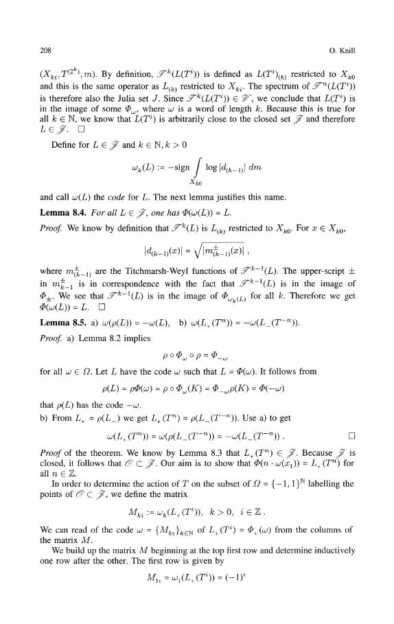
In order to determine the action of Γ on the subset of Ω = {— 1, 1}N labelling thepoints of ̂ C ̂ , we define the matrix

Mki :=ωk(L+(T1)), k > 0, ^ e Z .

We can read of the code ω = {Mkl}keN of L+ (Tl) = Φ+ (ω) from the columns ofthe matrix M.

We build up the matrix M beginning at the top first row and determine inductivelyone row after the other. The first row is given by

Mlt =^0^(7*)) = (-!)*


because T(XQl) = Xn and T(Xn) = XQl and

C r \ ί ί \I log|d(0)(z)| dm(x) = -sign / log|d(0)(z)| dm(x) .

/ \ */ /10 / V f l l /

The (fc + l)-th row can be constructed from the fc-th row using

T1)) , (4)

Proof of formula (4). We know from Φ+(L+) - L+ that d(/e_1) restricted to Xki isequal to d(k^ restricted to Xk+i2ί Therefore

wk+l (L+ (T2ϊ)) = -sign ί log \d(k}(T2ix}\ dm(x)

Xk+\,0

= -sign / log |d(fc)(a;)| dm(x)

Xk + \,2i

= -sign / log|d(A._υ(x)| dm(x)

Xk,τ

= -sign j logld^DCΓaOl rfrn(x) = wk(L+(T)) .

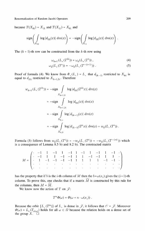
Formula (5) follows from wk(L+(Ti)) = -wk(L_(Tί)) = -wk(L+(T~ί+l)) whichis a consequence of Lemma 8.5 b) and 8.2 b). The constructed matrix

M =

ί - - 1 1 - 1 1 - 1 1 - 1 1 - 1 1 - 1 \- 1 1 1 - 1 - 1 1 1 - 1 - 1 1 1 •1 - 1 - 1 - 1 - 1 1 1 1 1 -1 -1

7

has the property that if 6 is the i-th column of M then the b + ω(xl) gives the (i+ l)-th

column. To prove this, one checks that if a matrix M is constructed by this rule for

the columns, then M - M.We know now the action of T on β?:

TnΦ(ω) = Φ(ω + n ω(xl)) .

Because the orbit {L+ (Tn)} of L+ is dense in ̂ , it follows that ̂ = ̂ . MoreoverΦ(ώ) - L+ (Tx(ω]) holds for all ω £ Ω because the relation holds on a dense set ofthe group X. D

210 O. Knill

9. The Density of States

There exists a probability measure dk in C satisfying for any / G C(R)

which is called the density of states of K. The next lemma gives the relation betweenthe density of states of the renormalized Jacobi operator Φ±L and the density of statesof the operator L.

Lemma 9.1. dk(Φ±L) = φ* dk(L).

Proof. Assume first that \X\ = TV is finite so that L is a TV-periodic Jacobi matrix.ι TV

Denote by dk(L) the Dirac measure — Σ ^(\)» where λ^ are the eigenvalues^ i=\

of L acting on the finite-dimensional vector space of TV periodic sequences in/2(Z). The 2TV x 2TV periodic Jacobi matrices D± = Φ±(L) have the eigenvalues

ά = 1 . This implies

[L)) = </>* dk(L) .

In the general case, let L^N\x) be a TV-periodic approximation of L(x) such that for-N/2<i,j < TV/2,

(HN\x)] i+NJ+N = [L(N\x)] {j = [L(x)] .,. .

By the lemma of Avron-Simon (see [Cyc]), one has the weak convergence

dk(L(N\x)) —> dk(L) for almost all xeX. The claim follows becauseΦ±(L(N\x)) —» Φ±(L(x)) in the weak operator topology. D

Proposition 9.2. The density of states of Φ(ω) is the unique equilibrium measure μon J.

Proof. We know that for (φ*)nv —> μ holds for any probability measure v on C, whereμ is the unique equilibrium measure on the Julia set J. Applying this to v - dk, thedensity of states of a Jacobi operator L, we get with Lemma 9.1

for all ω G Ω. The density of states of Φ(ω) is μ. D

Lemma 9.3. Every operator L = dτ + d(T~l)τ* G ̂ has the mass M(L) =exp (Jlog(d) dm = 1.

Proof. Because every element in $ has the same mass (Theorem 8.1), it is enoughto show that L+ = d+r + d+(T~l)τ* has mass 1. From the fixed point equationΦ+ (L+) = L+ we get ra+ (x)n+ (Tx) = d^ (x) for almost all x G X{. Using this, wecalculate

ί 1 f I fI log \d+ I dm = - log |m+ | dm + - / log |n+ | dm

X X{ Xλ

= - / log |(d+ )2| dm= log |d+ | dm = - / log |d+ | dm

x, x

Renormalization of Random Jacobi Operators 21 1

which implies log(M(L+ )) = / log \d+ \ dm = 0. Dx

Remark. The above proof shows log(M(0±(L))) = | log(M(L)) and the renormali-sation maps Φ± are also contractions in the stronger topology

d(L,K) =\\\L-K\\\ + |log(M(L)) -

and map an open set of operators with positive mass and spectrum in a connectedneighborhood of J into its interior.

The potential theoretical Green function g of a compact set K C C is a functiong : C — > R which is harmonic on C\K, vanishes on K and has the property thatg - log(z) is bounded near z = oo. The Green function exists for the Julia set J of t(see [M]).

Proposition 9.4. TTze Lyapunov exponent E ι-> λ(E) o/αn operator L e Jfr is equalto the Green function g(E) of the Julia set J. The Lyapunov exponent λ of L G $ isvanishing exactly on the spectrum J of L.

Proof. The density of states of L G β' is the equilibrium measure on the Julia set J(Proposition 9.2) and gives J the capacity 7(J) = 1 (see [Bro]). The integral

u(z) = - I log \z - E'\ dk(E')

is called the conductor potential. The relation between the conductor potential, theGreen function and the capacity is given by the formula

g(z) = -u(z) + log(7( J)) ,

(see [T] Theorem III, 37). Lemma 9.3 together with the Thouless formula λ(z) =/log \z — Ef\ dk(E') — log(M) gives u(z) - —\(z). It follows that the Lyapunovexponent λ is equal to the Green function g of the Julia set J, which is by definitionvanishing on the Julia set. D

Because oo is a super-attractive fixed point of the polynomial map t(z) = z2 + E,there exist new coordinates z - ζ(z), near oo satisfying

ζotoζ-l(z) = z2 .

The function ζ is called the Bottcher function of the polynomial t. (See for example[M].)

Corollary 9.5. The Bottcher function ζfor the polynomial t satisfies ζ(z) = det(L — z)for E in a neighborhood of oo. One has

det(L - (z2 + E)) = det(L - z)2 .

Proof. The Green function g can be expressed as g(z) = log \ζ(z)\. It follows from

Kω| = exp(λ(*)) = I exp(-™(*))| - | det(L - z)\

and the analyticity of ζ and det(L — z) near oo that ζ(z) = det(L — z). The knownidentity g(z) = g(z2 + E)/2 for the Green function g gives then

det(L - (z2 + E)) = det(L - z)2 . D

It follows from the structure of the Julia set that for the limit-periodic Jacobioperators in ̂ , there is an obvious gap-labelling :

212 O. Knill

Proposition 9.6. The integrated density of states of L G ̂ takes in the gaps exactlythe values I - 2~n with n G N and 0 < I < 2n.

Proof. We know from Proposition 9.2 that the density of states is the equilibriummeasure on J and so a balanced measure. The inverse of the map tn has 2n branchesφ(n^ labelled by 0 < j < 2n. Each of the sets φ(n^(J) has measure 2~n. If a gap ofL G $ has / sets φ(n^\J) to the left and 2n — / such sets to the right, the integrateddensity of states of this gap is / 2~n. D

General gap-labelling theorems for limit-periodic operators lead to the same result:it is known that the integrated density of states of an almost periodic Jacobi operatortakes the values in the frequency module ([DS] Theorem III.l). For limit-periodicoperators having as the hull the compact topological group G, the frequency moduleis the Z module generated by {a e R | e2πiα 6 0} (see [Bel]). Applying this in ourcase leads also to Proposition 9.6.

10. Generalisations and Questions

We discuss some generalizations or extensions:

Complex values E. Because an attractor of a hyperbolic iterated function system isstructurally stable, the renormalisation is defined on an open subset of C. All theresults about the density of states, the Green function, etc. hold also there.

Julia sets of the anti-holomorphic quadratic map. Operators with spectra on the Juliasets of z t— » t(z) = z2 + E (introduced by Milnor) can be obtained by replacing Φ± by

Φ± . The parameter set of ϊ analogous to the Mandelbrot set is called the Mandelbarset or tricorn.

Nonrandom Jacobi matrices. An advantage of doing the renormalisation for randomoperators over dynamical systems is that one gets immediately the dynamical systemover which the Jacobi operators are defined in the limit. We remark that for generalJacobi operators on /2(Z), there exists a continuum of Backlund transformationsBTS [GZ] parametrized by a parameter s e [—1,1]. For Random Jacobi operators,the random boundary condition selects two of them. It might be possible that therenormalisation for nonrandom Jacobi matrices can be done with an iterated functionsystem Φs parametrized by s G [— 1, 1].

Jacobi operators on the strip. The renormalization of Jacobi operators can begeneralized to some random Jacobi operators on the strip in the crossed product ofL°°(X,M(N,C)) with the dynamical system. In the limit of renormalisation, theseoperators factorize into a direct sum of one-dimensional operators, obtained there.

Higher-dimensional Laplacians. A direct generalization to higher- dimensional ran-dom Laplacians is not possible without further modifications. The reason is that fora Laplacian

the cocycles airi satisfy the zero curvature condition

a T r = 0


while the cocycles diσi belonging to the discrete Dίrac operator D = Σ ά%σi +

dί(S~l)σ^ must satisfy the anti-commutation relation %

{d^d^} = (dtd^SJ + d3di(Sj)}σiσj = 0, i ij

which prevents a further factorization of D unless one renormalises also the statistics.Dirac operators play a role when doing isospectral deformations of higher-dimensionalLaplacians [K3].

Operators with spectra on random Julia sets. The renormalization can be generalizedin another way. Instead of taking a constant energy E, we can take a space dependentfunction E(x) < — R for large enough R. We get again the same type of result asbefore. There exists an attractor above the von Neumann Kakutani system whichconsists of operators having the spectrum on random Julia sets (compare [FS]).

Operators with spectra on Julia sets of higher degree polynomials. By composing therenormalisation map Φ with a linear map of the form Φ bL = aL + b with α, b G R,

one can get operators with spectra on the Julia set of the polynomial (az + b)2 + Eor on the Julia set of finite products of different such polynomials. With —Ei largeenough or ai \ small enough, the renormalisation limits exist.

More general values ofE. We don't know how far one can explore the renormalizationfor general complex parameters E. The results of the literature mentioned in theintroduction suggest however that one can find an iterated function system for alarge set of E. For complex E, one has to deal with not normal operators. Anotherproblem is that for smaller values of |J5|, the norm of Φn(L) can blow up under therenormalisation steps even if the spectrum converges to the Julia set. The reason isthat E can get closer and closer to the auxiliary spectrum of the matrices. Since theTitchmarsh-Weyl functions are singular at the auxiliary spectrum, the norm can getlarge or explode. Numerical investigations suggest that for all E in the complementof the Mandelbrot set, there should exist a hyperbolic iterated function system havinga Cantor set as an attractor. The scheme can not work for general E G C becausefor E - 0, a fixed point of D ι-+ Φ+ (D) = ψ(D2) is not almost-periodic. If we dothe renormalisation maps numerically for values E approaching 0, there are entriesin the Jacobi matrix which begin to blow up. Obviously an invariant set exists but itis no more an attractor.

The case E = — 2 is interesting because it describes a situation, where the energyE is at the boundary of the Mandelbrot set. The spectrum [—2,2] is then absolutelycontinuous with respect to the Lebesgue measure and the corresponding operator isthe free Laplacian. Numerically, the renormalisation maps are contractions for all realvalues E < -2 and the attractor $ approaches a single point in the limit E = -2.

We mention some open points:

• An obvious problem is to determine the maximal set in C, where the renormalisationmappings Φ± make sense and to understand what happens at the boundary of thismaximal set. Even if a fixed point L+ of the renormalisation map Φ+ exists, it isan additional problem to determine its stability or to check if Φ+ is a contraction.The key problem is to estimate the Frechet derivative of the Backlund transformationBT+ which we were only able to estimate for large \E\.

• The constructed operators have the property that the density of states is the potentialtheoretical equilibrium measure minimizing the energy on the spectrum. For whichrandom operators is this also true?

214 O. Knill

• The high symmetry of the constructed operators in $> could allow to determine theisospectral set of such operators. It is tempting to guess that the embedding of thedyadic group G in the infinite-dimensional torus Tω corresponds to an embeddingof the attractor β" in a not yet explored isospectral set of L+ which would then belabelled by the infinite-dimensional torus Tω.

Acknowledgement. I thank O. Lanford III for his support and valuable discussions.

References

[Bak] Baker, G.A., Bessis, D., Moussa, P.: A family of almost periodic Schrodinger operators.Physica A 124, 61-78 (1984)

[BGH1] Barnsley, M.F., Geronimo, J.S., Harrington, A.N.: Geometry, electrostatic measure andorthogonal polynomials on Julia sets for polynomials. Erg. Th. Dynam. Sys. 3, 509-520(1983)

[BGH2] Barnsley, M.F., Geronimo, J.S., Harrington, A.N.: Infinite-Dimensional Jacobi matricesassociated with Julia sets. Proc. Am. Math. Soc. 88, 625-630 (1983)

[BGH3] Barnsley, M.F., Geronimo, J.S., Harrington, A.N.: Almost periodic Jacobi matrices associ-ated with Julia sets for polynomials. Commun. Math. Phys. 99, 303-317 (1985)

[Bar] Barnsley, M.: Fractals everywhere., London: Academic Press 1988[BBM] Bellissard, J., Bessis, D., Moussa, P.: Chaotic states of almost periodic Schrodinger

operators. Phys. Rev. Lett. 49, 700-704 (1982)[Bel] Bellissard, J.: Gap labelling theorems for Schrodinger operators. In: Waldshmidt et al. (ed.)

From Number theory to physics. Berlin, Heidelberg, New York: Springer 1982[BGM] Bessis, D., Geronimo, J.S., Moussa, P.: Function weighted measures and orthogonal

polynomials on Julia sets. Constr. Approx. 4, 157-173 (1988)[BMM] Bessis, D., Mehta, M.L., Moussa, P.: Orthogonal polynomials on a family of Cantor sets

and the problem of iterations of quadratic mappings. Lett. Math. Phys. 6, 123-140 (1982)[Bla] Blanchard P.: Complex analytic dynamics on the Riemann sphere. Bull. (New Ser.) of the

Am. Math. Soc. 11, 85-141 (1984)[Bro] Brolin H.: Invariant sets under iteration of rational functions. Arkiv Math. 6, 103-144

(1965)[CG] Carleson, L., Gamelin, T.W.: Complex dynamics. Springer: Berlin, Heidelberg, New York

1993[CL] Caπnona, R., Lacroix, J.: Spectral theory of random Schrodinger operators. Boston:

Birkhauser, 1990[C] Chulaevsky, V.A.: Almost periodic operators and related nonlinear integrable systems.

Manchester: Manchester University Press 1989[CFS] Cornfeld, I.P., Fomin, S.V., Sinai, Ya.G.: Ergodic theory. Berlin, Heidelberg, New York:

Springer 1982[CFKS] Cycon, H.L., Froese, R.G., Kirsch, W., Simon, B.: Schrodinger operators. Texts and

Monographs in Physics. Berlin, Heidelberg, New York: Springer 1987[DS] Delyon, F., Souillard, B.: The rotation number for finite difference operators and its

properties. Commun. Math. Phys. 89, 415-426 (1983)[EL] Eremenko, A., Lyubich, M.: The dynamics of analytic transformations. Leningrad Math. J.

3, 563-634 (1990)[FT] Faddeev, L.D.,Takhtajan, L.A.: Hamΐltonian methods in the theory of solitons. Berlin,

Heidelberg, New York: Springer 1986[FS] Fornaess, J., Sibony N.: Random iterations of rational functions. Ergod. Th. Dynam. Sys.

11, 687-708 (1991)[F] Friedman, N.A.: Replication and stacking in ergodic theory. Am. Math. Monthly, January

1992[GZ] Gesztesy, F., Zhao, Z.: Critical and subcritical Jacobi operators defined as Friedrichs

extensions. J. Diff. Eq. 103, 68-93 (1993)[H] Halmos, P.: Lectures on ergodic theory. The Mathematical Society of Japan, Tokyo, 1956


[Kl] Knill, O.: Isospectral deformations of random Jacobi operators. Commun. Math. Phys. 151,403-426 (1993)

[K2] Knill, O.: Factorisation of random Jacobi operators and Backlund transformations. Commun.Math. Phys. 151, 589-605 (1993)

[K3] Knill, O.: Isospectral deformation of discrete random Laplacians. To appear in theProceedings of the Workshop "Three Levels," Leuven, July 1993

[L] Ljubich, MJu.: Entropy properties of rational endomorphisms of the Riemann sphere.Ergod. Th. Dynam. Sys. 3, 351-385 (1983)

[McK] McKean, H.P.: Is there an infinite dimensional algebraic geometry? Hints from KdV. Proc.of Symposia in Pure Mathematics 49, 27-38 (1989)

[M] Milnor, J.: Dynamics in one complex variable. Introductory Lectures, SUNY, 1991[P] Parry, W.: Topics in ergodic theory. Cambridge: Cambridge University Press, 1980[PF] Pastur, L., Figotin A.: Spectra of random and almost-periodic operators. Grundlehren der

mathematischen Wissenschaften 297. Berlin, Heidelberg, New York: Springer 1992[Per] Perelomov, A.M.: Integrable Systems of classical Mechanics and Lie Algebras. Birkhauser,

Boston, 1990[Tod] Toda, H.: Theory of nonlinear lattices. Berlin, Heidelberg, New York: Springer 1981[T] Tsuji, M.: Potential theory in modern function theory. New York: Chelsea Publishing

Company 1958

Communicated by B. Simon

Documents

Renormalization of Random Jacobi Operatorsknill/offprints/renormalization.pdf · Renormalization of Random Jacobi Operators 197 J of the quadratic map z ι-» z2 + E. Moreover, we