Renormalization group method for construction of the

1

Renormalization group method for

construction of the invariant manifold and

its application to a resolution of

Hilbert’s sixth problem with quantum statistics

Teiji Kunihiro Dep. Physics, Kyoto U.

Hilbert’s 6th problem,

University of Leicester, May 02 -04, 2016

based on work done with S. Ei, K. Fujii, and K. Ohnishi, K.Tsumura and Y. Kikuchi

2

Contents

1. Introduction: Geometrical formulation of reduction of dynamics

2. Renormalization group method for constructing the asymptotic invariant/attractive manifold 3. Application of the RG method for derivation of the 2nd-order (non-)relativistic hydrodynamics with quantum statistics 4. Example: cold fermionic atoms and validity test of the relaxation-time (BGK) approximation 5. Brief summary and concluding remarks

3

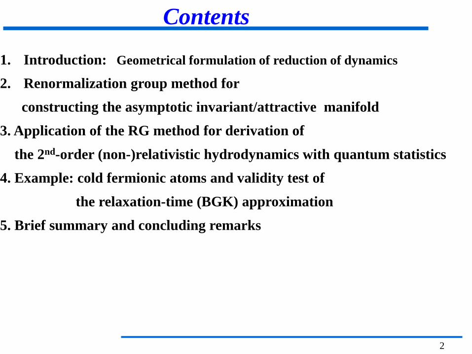
Separation of scales in the time evolution of a physical system Liouville Kinetic (Boltzmann eq.) Fluid dyn.

Hamiltonian

Slower dynamics with fewer variables

Introduction

(BBGKY hierarchy) One-body dist. fn. Hydrodynamic variables, T ,n and so on uµ

(i) From Liouville (BBGKY) to Boltzmann (Bogoliubov) The relaxation time of the s-body distribution function F_s (s>1) should be short and hence slaving variables of F_1. The reduced dynamics is described solely with the one-body distribution function F_1 as.the coordinate of the attractive manifold. N.N. Bogoliubov, in “Studies in Statistical Mechanics”, (J. de Boer and G. E. Uhlenbeck, Eds.) vol2, (North-Holland, 1962) (ii) Boltzmann to hydrodynamics (Hilbert, Chapman-Enskog,Bogoliubov

After some time, the one-body distribution function is asymptotically well described by local temperature T(x), density n(x), and the flow velocity u , i.e., the hydrodynamic variables

(iii) Langevin to Fokker-Planck equation, (iv) Critical dynamics as described by TDGL etc…..

(i) (ii)

4

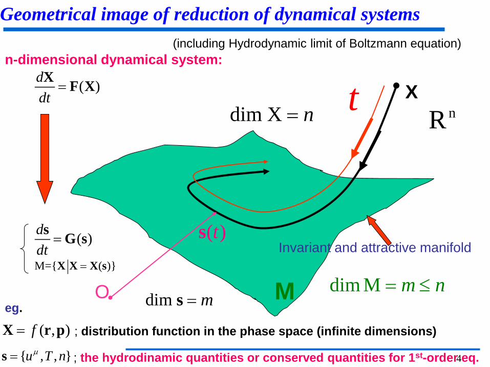
Geometrical image of reduction of dynamical systems

nR∞∞

t X

M dim M m n= ≤

dim X n=

( )ts

O dim m=s

Invariant and attractive manifold

( )ddt

=X F X

( )ddt

=s G s

M={ ( )}=X X X s

( , )f=X r p ; distribution function in the phase space (infinite dimensions)

{ , , }u T nµ=s ; the hydrodinamic quantities or conserved quantities for 1st-order eq.

eg.

n-dimensional dynamical system: (including Hydrodynamic limit of Boltzmann equation)

5

The problems listed above maybe formulated as a construction of asymptotic invariant/attractive manifold

with a possible space-time coarse-graining, and

it may be interpreted as a geometrical resolution to Hilbert’s 6th problem,

which is based on the similarity of geometry and physics.

c.f. Leo Corry’s talk; Arch. Hist. exact. Sci. 51 (1997) 83.

Introduction (continued)

6

We adopt the RG method (Chen et al, 1995; T.K. (1995)) to construct the attractive/invariant manifolds and extend it so as to incorporate excited modes as well as the would-be zero modes as the slow/collective variables and thereby derive the second-order hydrodynamics as the mesoscopic dynamics. K. Tsumura and T.K., EPJA 48 (2012), 162 :Announcement K. Tsumura, Y. Kikuchi and TK, arXiv:1311.7059; Non-rel and classical TKT, PRD92 (2015); Quantum and relativistic with single component Y. Kikuchi, K.Tsumura and TK, PRC92 (2015); Quantum and relativistic with multiple reactive components Y. Kikuchi, K. Tsumura and TK, PLA380 (2016), 2075; Quantum and non-rel with application to cold fermionic gas. See also, Y. Kikuchi, K. Tsumura and TK, arXiv:1604.07458.

The Purpose of this talk

K. Tsumura, K. Ohnishi and TK, PLB46 (2007), 134: 1st-order eq.

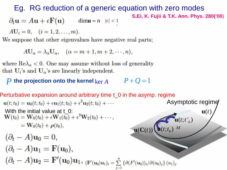
Eg. RG reduction of a generic equation with zero modes S.Ei, K. Fujii & T.K. Ann. Phys. 280(’00)

P the projection onto the kernel ker A 1P Q+ =

Perturbative expansion around arbitrary time t_0 in the asymp. regime

With the initial value at t_0: Asymptotic regime

( )tu

( ( ))tu C 0( ; )t tu0( ; ' )t tu

dim n=u

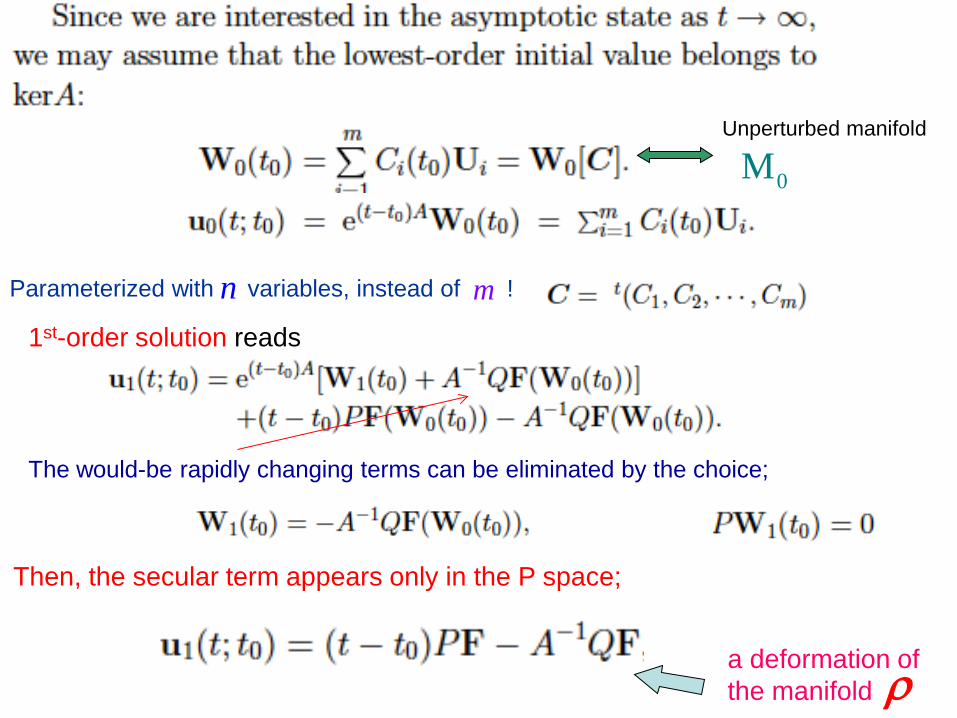
Parameterized with variables, instead of ! mn

The would-be rapidly changing terms can be eliminated by the choice;

Then, the secular term appears only in the P space;

a deformation of the manifold

0M

ρ

1st-order solution reads

Unperturbed manifold

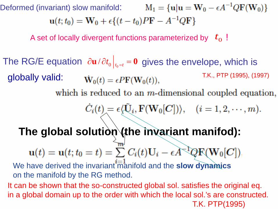
Deformed (invariant) slow manifold:

The RG/E equation 00/ t tt =∂ ∂ =u 0 gives the envelope, which is

The global solution (the invariant manifod):

We have derived the invariant manifold and the slow dynamics on the manifold by the RG method.

A set of locally divergent functions parameterized by ! 0t

globally valid: T.K., PTP (1995), (1997)

It can be shown that the so-constructed global sol. satisfies the original eq. in a global domain up to the order with which the local sol.’s are constructed. T.K. PTP(1995)

Extensions

Aa) is not semi-simple.with Jordan cell b) Higher orders.

Y. Hatta and T.K. Ann. Phys. (2002)

Layered pulse dynamics for TDGL and Non-lin.Schroedinger.

c) PD equations;

d) Reduction of stochastic equation with several variables; Liouville to Boltzmann, Langevin to Focker-Plank: Further reduction of F-P with hierarchy of time scales. e) Discrete systems

S. Ei, K. Fujii and T.K. , Ann.Phys.(’00)

See also, T.K.,Jpn. J. Ind. Appl. Math. 14 (’97), 51

T.K. and J. Matsukidaira, Phys. Rev. E57 (’98), 4817

f) Derivation of hydrodynamic limit of Boltzmann eq. in classical/quantum (non) relativistic (reactive multicomponent) systems

11

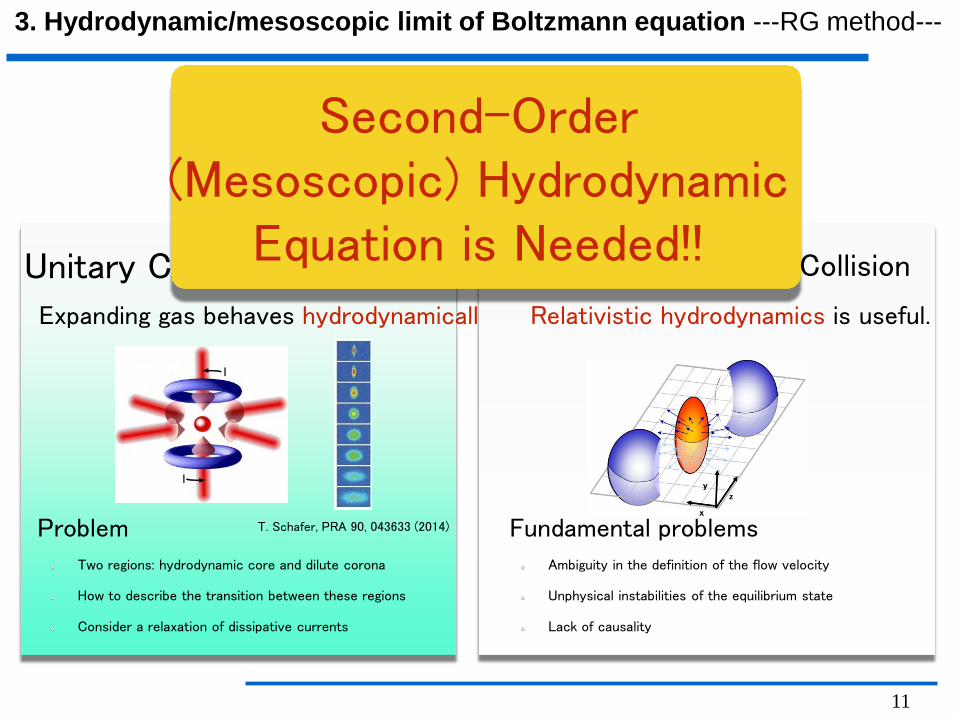
3. Hydrodynamic/mesoscopic limit of Boltzmann equation ---RG method---

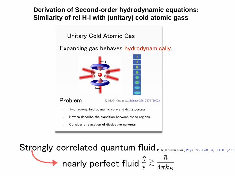
Unitary Cold Atomic Gas

T. Schafer, PRA 90, 043633 (2014)

Expanding gas behaves hydrodynamically.

Two regions: hydrodynamic core and dilute corona

How to describe the transition between these regions

Consider a relaxation of dissipative currents

Problem

Relativistic hydrodynamics is useful.

Ambiguity in the definition of the flow velocity

Unphysical instabilities of the equilibrium state

Lack of causality

Relativistic Heavy Ion Collision

Fundamental problems

Second-Order (Mesoscopic) Hydrodynamic

Equation is Needed!!

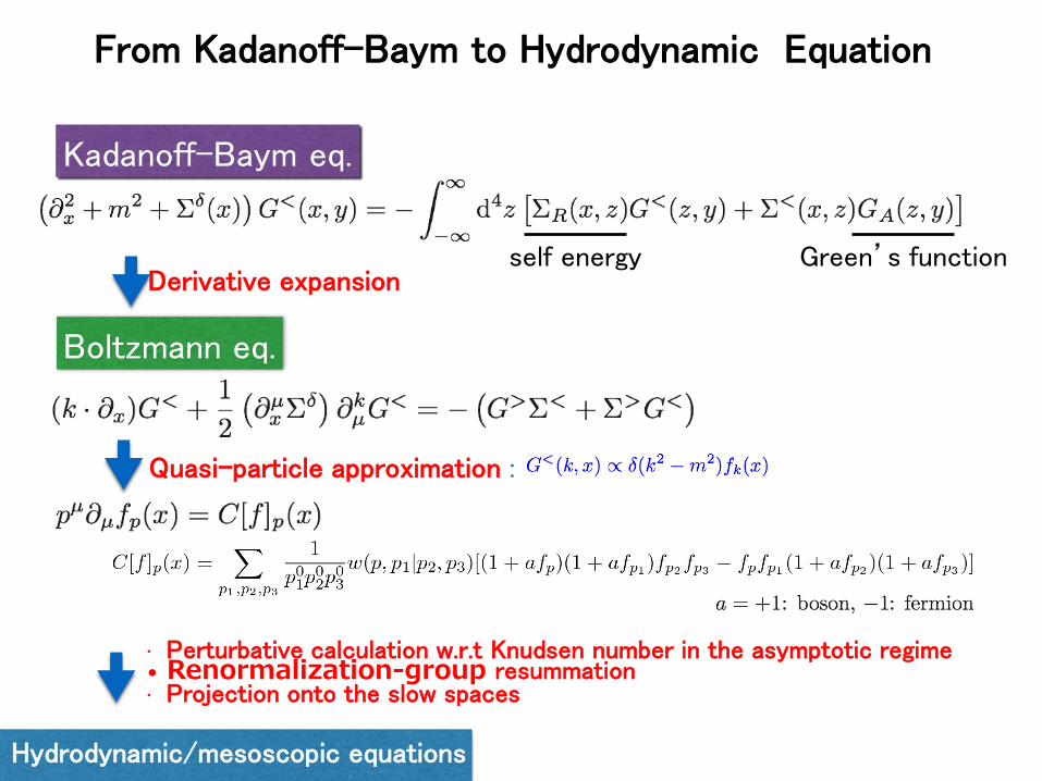
Kadanoff-Baym eq.

Boltzmann eq.

Derivative expansion

Quasi-particle approximation :

• Perturbative calculation w.r.t Knudsen number in the asymptotic regime • Renormalization-group resummation • Projection onto the slow spaces

Green’s function self energy

From Kadanoff-Baym to Hydrodynamic Equation

Hydrodynamic/mesoscopic equations

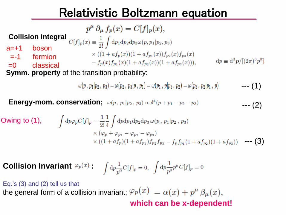
Relativistic Boltzmann equation

--- (1)

Collision integral:

Symm. property of the transition probability:

Energy-mom. conservation; --- (2)

Owing to (1),

--- (3)

Collision Invariant :

the general form of a collision invariant; which can be x-dependent!

Eq.’s (3) and (2) tell us that

a=+1 boson =-1 fermion =0 classical

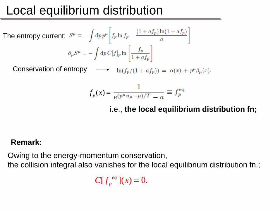
The entropy current:

Conservation of entropy

i.e., the local equilibrium distribution fn;

Local equilibrium distribution

Owing to the energy-momentum conservation, the collision integral also vanishes for the local equilibrium distribution fn.;

Remark:

[ ]( ) 0.eqpC f x =

( )pf x =

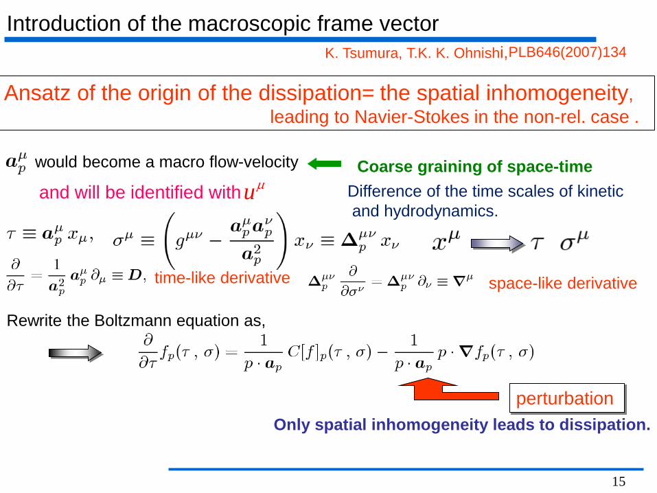
15

perturbation

Ansatz of the origin of the dissipation= the spatial inhomogeneity, leading to Navier-Stokes in the non-rel. case .

would become a macro flow-velocity

Introduction of the macroscopic frame vector K. Tsumura, T.K. K. Ohnishi, PLB646(2007)134

time-like derivative space-like derivative

Rewrite the Boltzmann equation as,

Only spatial inhomogeneity leads to dissipation.

Coarse graining of space-time and will be identified with uµ Difference of the time scales of kinetic

and hydrodynamics.

16

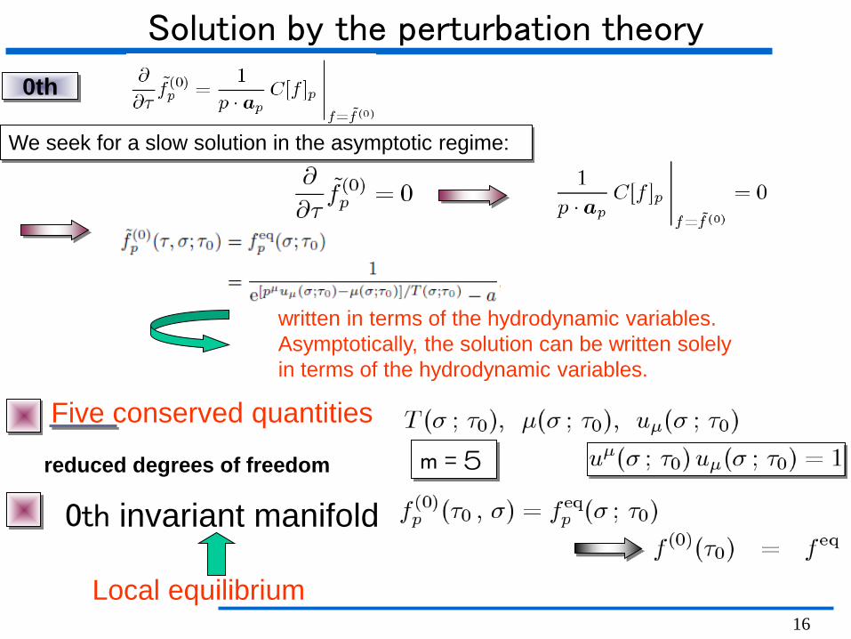
Solution by the perturbation theory

0th

0th invariant manifold

We seek for a slow solution in the asymptotic regime:

Five conserved quantities m = 5

Local equilibrium

reduced degrees of freedom

written in terms of the hydrodynamic variables. Asymptotically, the solution can be written solely in terms of the hydrodynamic variables.

17

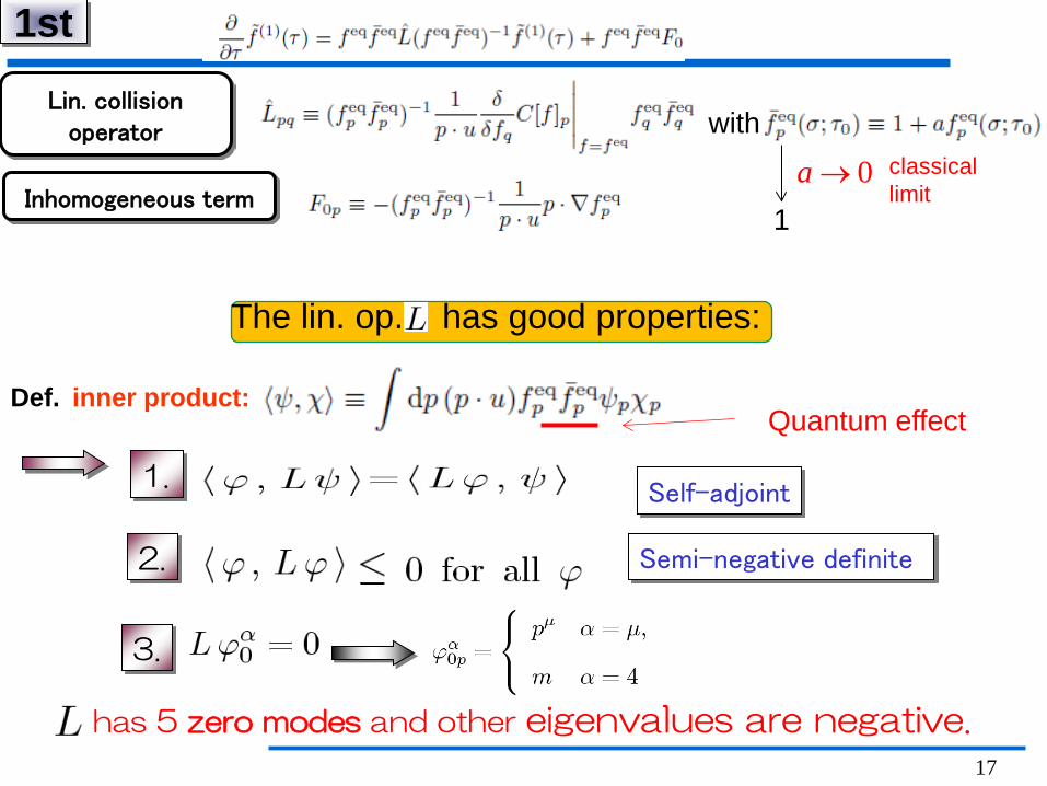
1st

The lin. op. has good properties:

Lin. collision operator

1. Self-adjoint

2. Semi-negative definite

3.

has 5 zero modes and other eigenvalues are negative.

Def. inner product:

with

Inhomogeneous term

Quantum effect

1 0a → classical

limit

18

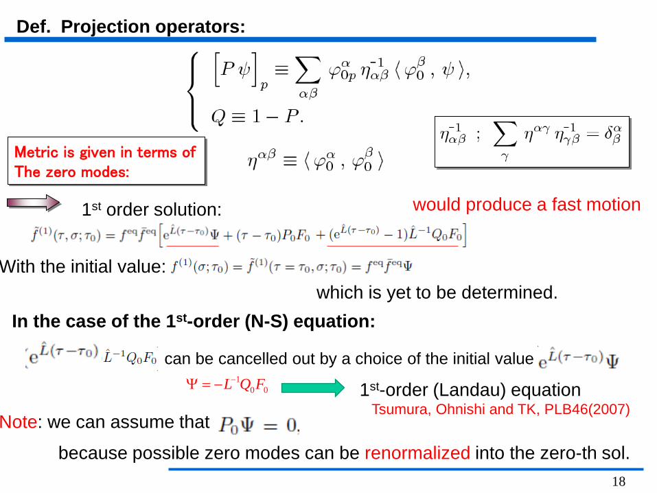
Metric is given in terms of The zero modes:

Def. Projection operators:

1st order solution:

With the initial value:

Note: we can assume that

which is yet to be determined.

because possible zero modes can be renormalized into the zero-th sol.

In the case of the 1st-order (N-S) equation:

would produce a fast motion

can be cancelled out by a choice of the initial value 1

0 0L Q F−Ψ = − 1st-order (Landau) equation Tsumura, Ohnishi and TK, PLB46(2007)

: small

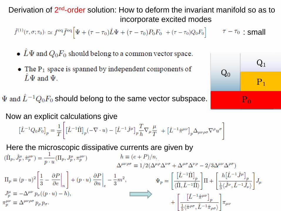
Derivation of 2nd-order solution: How to deform the invariant manifold so as to incorporate excited modes

should belong to the same vector subspace.

Now an explicit calculations give

Here the microscopic dissipative currents are given by

16/24

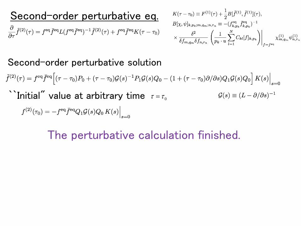
Second-order perturbative solution

``Initial" value at arbitrary time

The perturbative calculation finished.

Yuta Kikuchi (Kyoto U.) Second-order perturbative eq.

0τ τ=

18/24

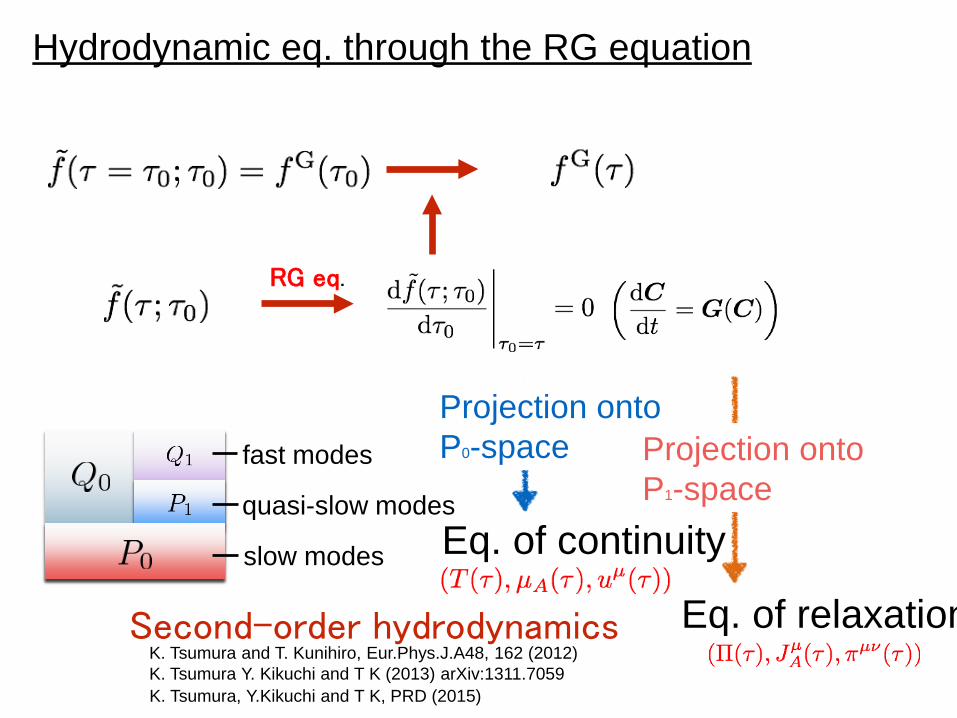
Eq. of continuity

Eq. of relaxation slow modes

quasi-slow modes

fast modes

Second-order hydrodynamics

Projection onto P0-space Projection onto

P1-space

Yuta Kikuchi (Kyoto U.)

K. Tsumura and T. Kunihiro, Eur.Phys.J.A48, 162 (2012) K. Tsumura Y. Kikuchi and T K (2013) arXiv:1311.7059 K. Tsumura, Y.Kikuchi and T K, PRD (2015)

Hydrodynamic eq. through the RG equation

RG eq.

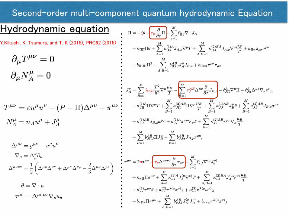
21/24 11/17 20/24 15/17 Second-order multi-component quantum hydrodynamic Equation

Hydrodynamic equation Y.Kikuchi, K. Tsumura, and T. K (2015), PRC92 (2015)

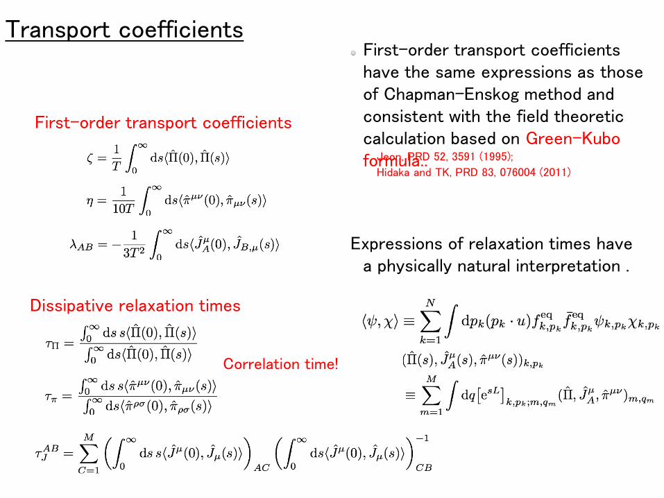
12/17 21/24 11/17 20/24 15/17 21/24 Yuta Kikuchi (Kyoto U.) Transport coefficients

First-order transport coefficients have the same expressions as those of Chapman-Enskog method and consistent with the field theoretic calculation based on Green-Kubo formula..

Expressions of relaxation times have a physically natural interpretation .

First-order transport coefficients

Dissipative relaxation times

Hidaka and TK, PRD 83, 076004 (2011)

Jeon, PRD 52, 3591 (1995);

Correlation time!

07/15

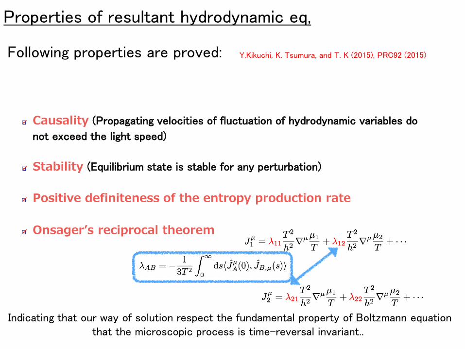
Causality (Propagating velocities of fluctuation of hydrodynamic variables do

not exceed the light speed)

Stability (Equilibrium state is stable for any perturbation)

Positive definiteness of the entropy production rate

Onsager’s reciprocal theorem

16/17 22/24

Following properties are proved:

Yuta Kikuchi (Kyoto U.) Properties of resultant hydrodynamic eq,

Y.Kikuchi, K. Tsumura, and T. K (2015), PRC92 (2015)

Indicating that our way of solution respect the fundamental property of Boltzmann equation that the microscopic process is time-reversal invariant..

04/17 03/24 Yuta Kikuchi (Kyoto U.) 02/22

Yuta Kikuchi (Kyoto U.)

Unitary Cold Atomic Gas

Expanding gas behaves hydrodynamically.

Two regions: hydrodynamic core and dilute corona

How to describe the transition between these regions

Consider a relaxation of dissipative currents

Problem K. M. O’Hara et al., Science 298, 2179 (2002)

Strongly correlated quantum fluid

nearly perfect fluid :

P. K. Kovtun et al., Phys. Rev. Lett. 94, 111601 (2005

Derivation of Second-order hydrodynamic equations: Similarity of rel H-I with (unitary) cold atomic gass

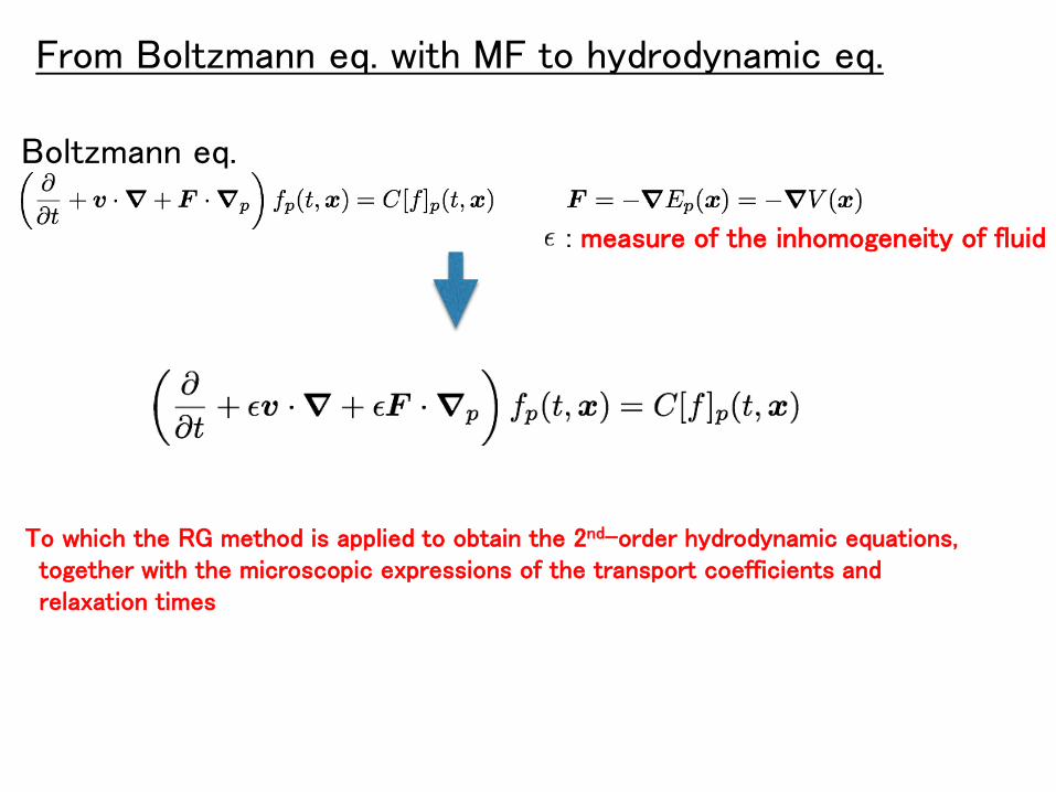
: measure of the inhomogeneity of fluid

Boltzmann eq.

08/17 10/24 13/17 10/24 Yuta Kikuchi (Kyoto U.) 21/26 07/17

Yuta Kikuchi (Kyoto U.) From Boltzmann eq. with MF to hydrodynamic eq.

08/22

To which the RG method is applied to obtain the 2nd-order hydrodynamic equations, together with the microscopic expressions of the transport coefficients and relaxation times

07/15 16/17 13/22 Yuta Kikuchi (Kyoto U.)

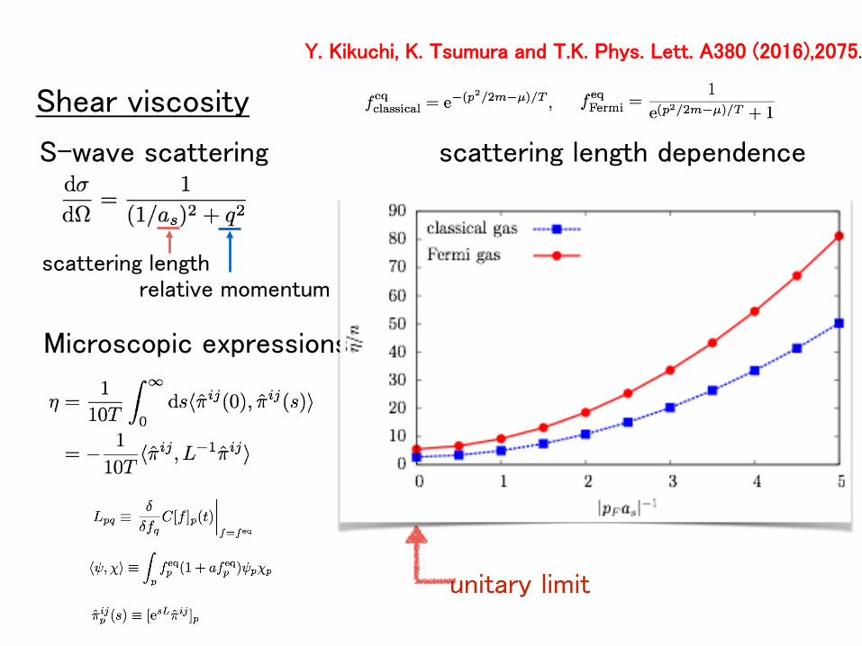
Shear viscosity

unitary limit

Microscopic expressions

S-wave scattering

relative momentum scattering length

scattering length dependence

Y. Kikuchi, K. Tsumura and T.K. Phys. Lett. A380 (2016),2075.


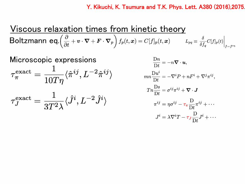
Viscous relaxation times from kinetic theory

Microscopic expressions

Boltzmann eq.


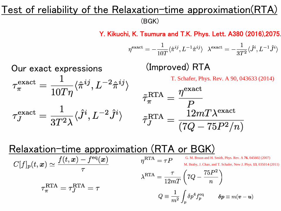
07/15 16/17 18/22 Yuta Kikuchi (Kyoto U.) Test of reliability of the Relaxation-time approximation(RTA)

Our exact expressions

Relaxation-time approximation (RTA or BGK)

(Improved) RTA

G. M. Bruun and H. Smith, Phys. Rev. A 76, 045602 (2007)

M. Braby, J. Chao, and T. Schafer, New J. Phys. 13, 035014 (2011)

T. Schafer, Phys. Rev. A 90, 043633 (2014)


(BGK)

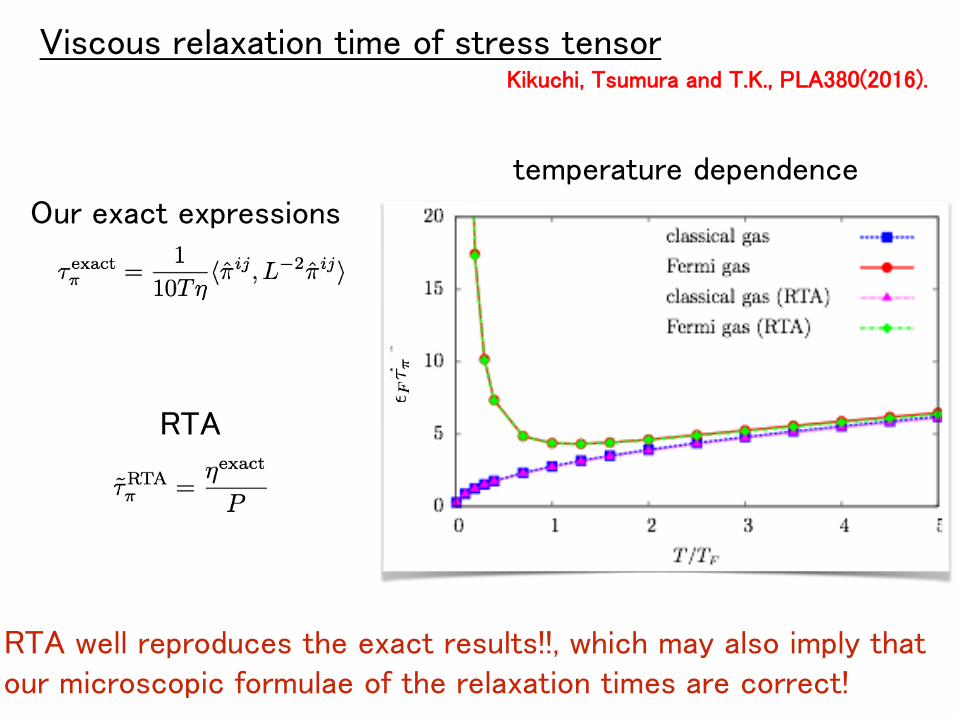
07/15 16/17 19/22 Yuta Kikuchi (Kyoto U.) Viscous relaxation time of stress tensor

temperature dependence

RTA

Our exact expressions

RTA well reproduces the exact results!!, which may also imply that our microscopic formulae of the relaxation times are correct!

Kikuchi, Tsumura and T.K., PLA380(2016).

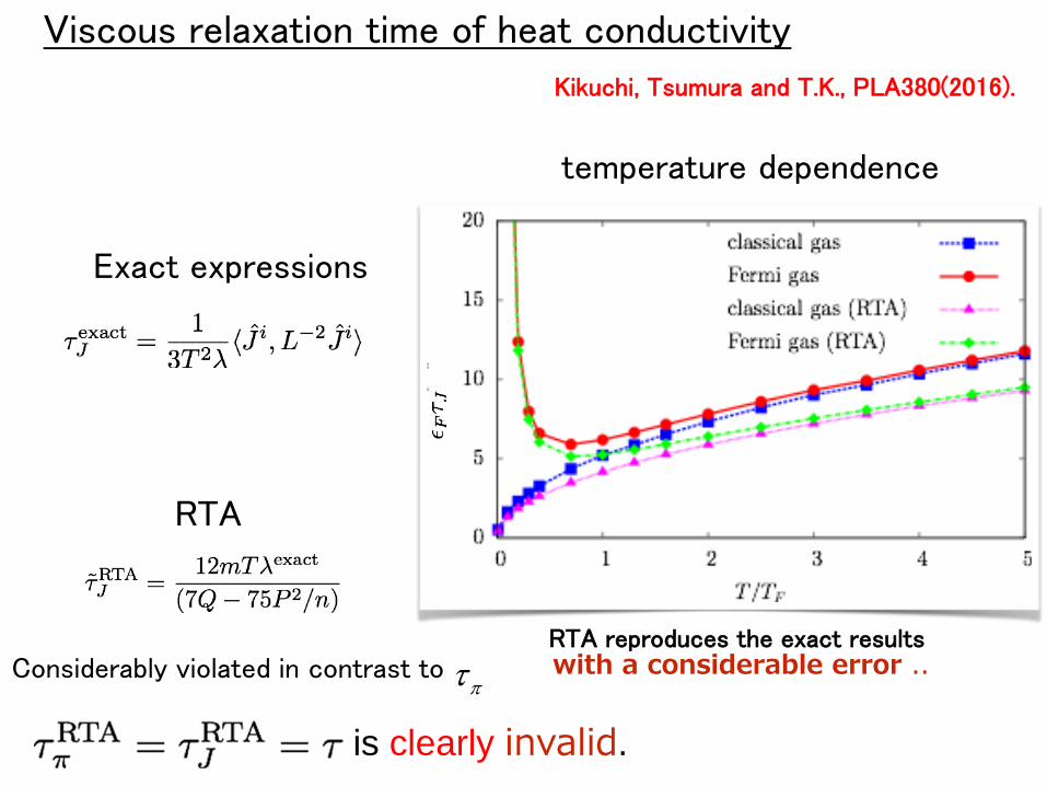
07/15 16/17 20/22 Yuta Kikuchi (Kyoto U.) Viscous relaxation time of heat conductivity

temperature dependence

RTA reproduces the exact results with a considerable error ..

RTA

Exact expressions

is clearly invalid.

Considerably violated in contrast to πτ

Kikuchi, Tsumura and T.K., PLA380(2016).

32

07/15

A geometrical formulation of the reduction of the dynamics is given on the basis of the renormalization-group/envelope method, which may give a partial and intermediate resolution of Hilbert’s 6th problem. variational principle (Hilbert)?

The microscopic expressions of the transport coefficients that coincide with those of Chapman-Enskog and viscous relaxation times are derived from the Boltzmann equation (quasi-particle approx.) by an adaptation of the RG method, and numerical evaluations are perfomed without recourse to any approximation.

Quantum statistics makes significant contributions to the shear viscosity (and the others as well).

We have numerically examined that the relation ,which is derived in the RTA, is satisfied quite well.

The analogous relation for is satisfied only approximately.

For a realistic cal. of transport coeff.’s, Kadanoff-Baym formalism with off-shell effects or wave-coherence included may be useful.

Summary 16/17 22/22

L.P. Kadanoff and G. Baym ‘Quantum Statistical Mechanics’ (1962, Benjamin)

Back Ups

11/17

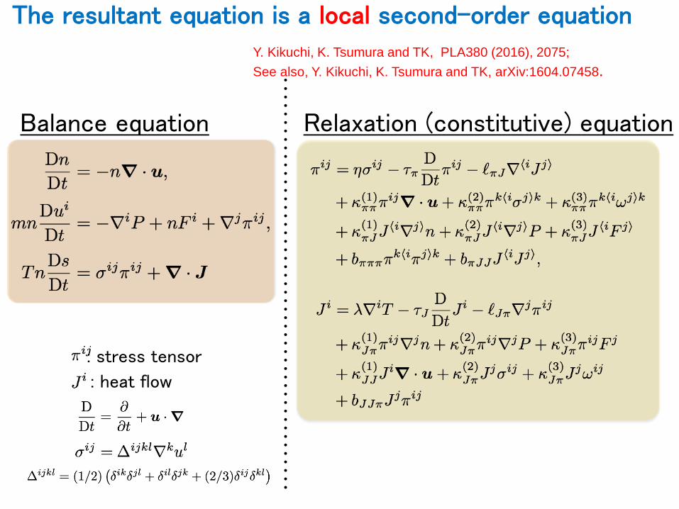
: stress tensor

: heat flow


Balance equation Relaxation (constitutive) equation

Y. Kikuchi, K. Tsumura and TK, PLA380 (2016), 2075; See also, Y. Kikuchi, K. Tsumura and TK, arXiv:1604.07458.

The resultant equation is a local second-order equation

35

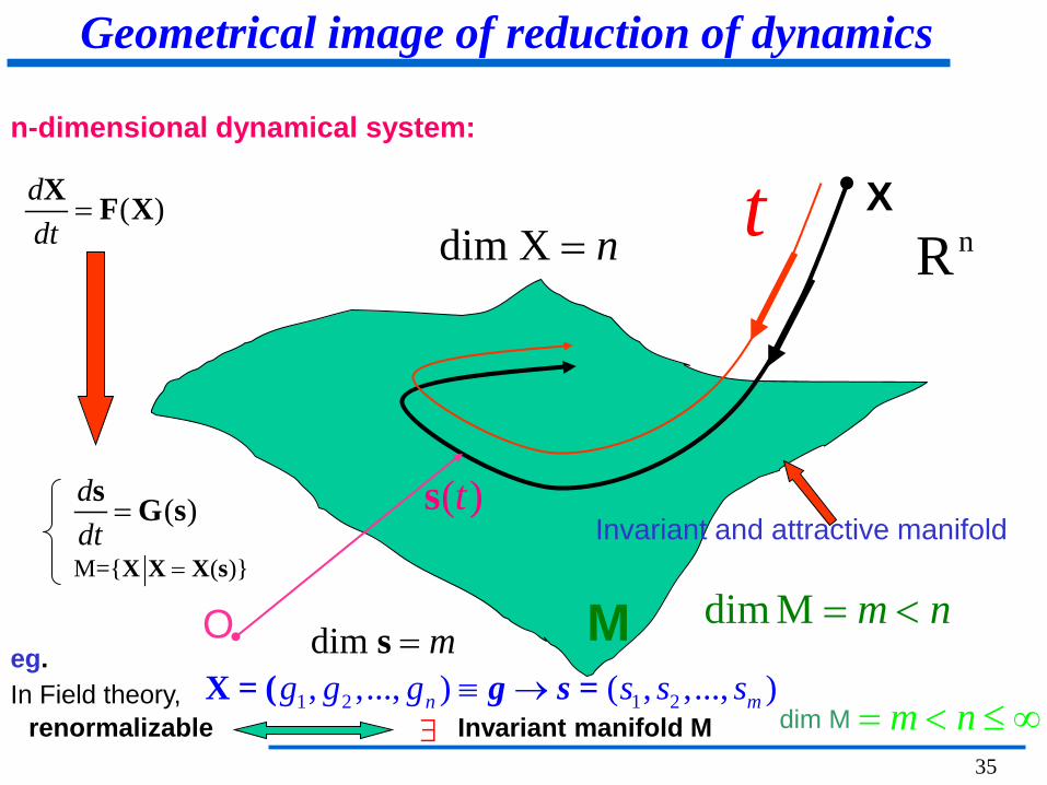
Geometrical image of reduction of dynamics

nR∞∞

t X

M dim M m n= <

dim X n=

( )ts

O dim m=s

Invariant and attractive manifold

( )ddt

=X F X

( )ddt

=s G s

M={ ( )}=X X X s

eg. 1 2 1 2, ,..., ) ( , ,..., )n mg g g s s s≡ →X = ( g s =In Field theory,

renormalizable ∃ Invariant manifold M dim M m n= < ≤ ∞

n-dimensional dynamical system:

36

The RG/flow equation

The yet unknown function is solved exactly and inserted into

Γ , which then becomes valid in a global domain of the energy scale.

g

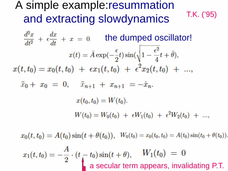
A simple example:resummation and extracting slowdynamics

T.K. (’95)

a secular term appears, invalidating P.T.

the dumped oscillator!

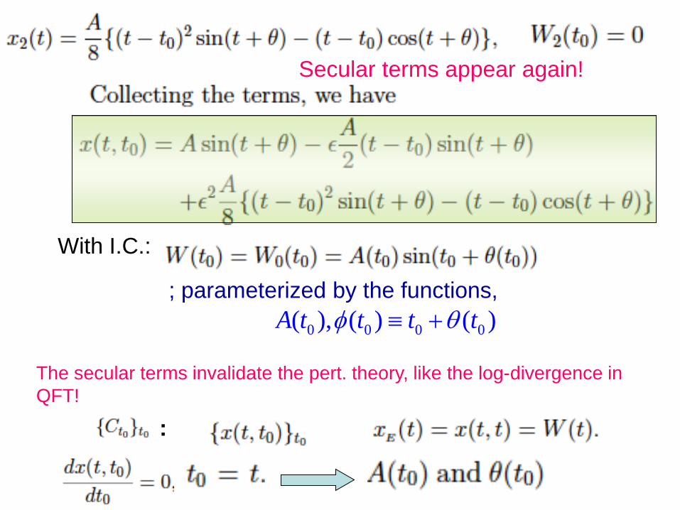
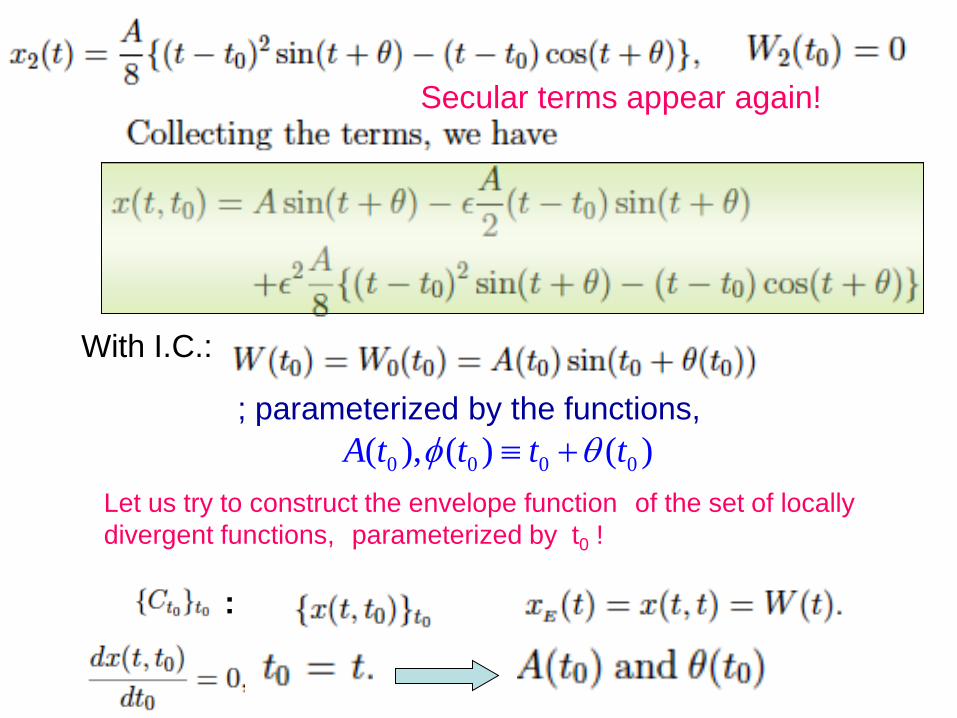
; parameterized by the functions, 0 0 0 0( ), ( ) ( )A t t t tφ θ≡ +

:

Secular terms appear again!

With I.C.:

The secular terms invalidate the pert. theory, like the log-divergence in QFT!

; parameterized by the functions, 0 0 0 0( ), ( ) ( )A t t t tφ θ≡ +

:

Secular terms appear again!

With I.C.:

Let us try to construct the envelope function of the set of locally divergent functions, parameterized by t0 !

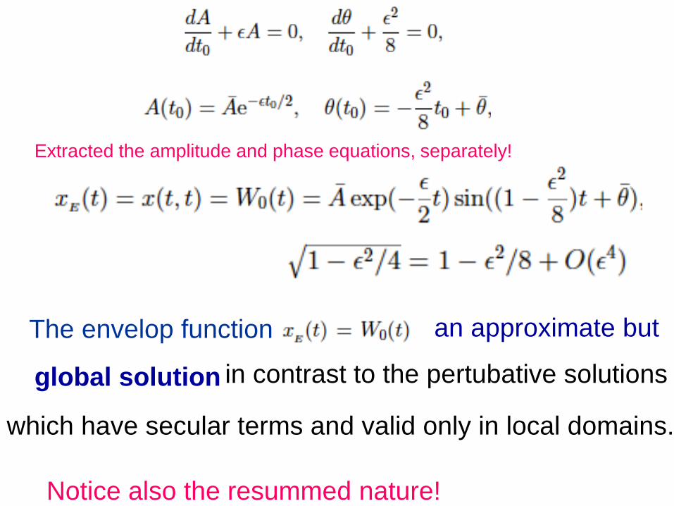
The envelop function an approximate but global solution in contrast to the pertubative solutions

which have secular terms and valid only in local domains.

Notice also the resummed nature!

Extracted the amplitude and phase equations, separately!

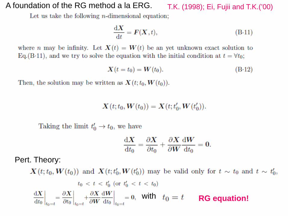
Pert. Theory:

with RG equation!

A foundation of the RG method a la ERG. T.K. (1998); Ei, Fujii and T.K.(’00)

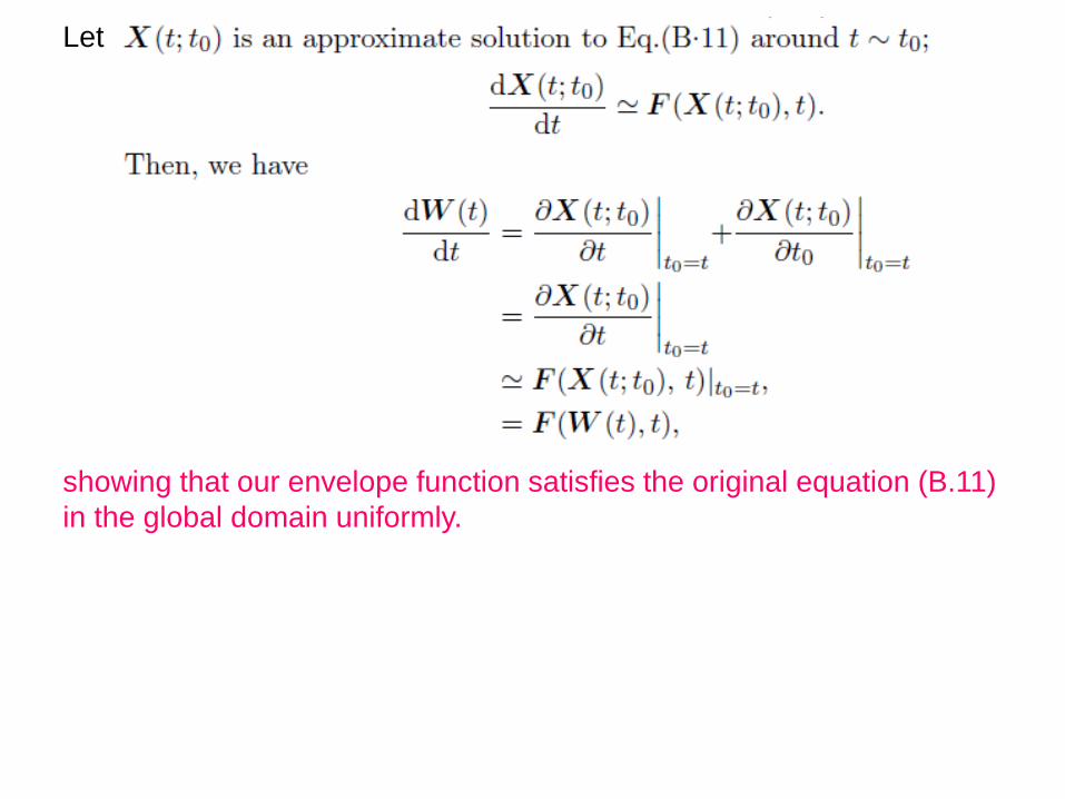
Let

showing that our envelope function satisfies the original equation (B.11) in the global domain uniformly.

43

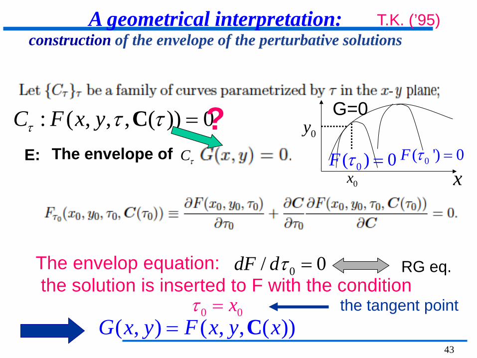
A geometrical interpretation: construction of the envelope of the perturbative solutions

: ( , , , ( )) 0C F x yτ τ τ =CThe envelope of CτE:

?

The envelop equation: the solution is inserted to F with the condition

0 0xτ =( , ) ( , , ( ))G x y F x y x= C

the tangent point

RG eq. 0/ 0dF dτ =

T.K. (’95)

G=0

0( ) 0F τ = 0( ') 0F τ =

x0x

0y

Documents

Renormalization group method for construction of the