Embed Size (px)
Citation preview

Renormalization Group Approach
to Hot and Dense Matter
Vom Fachbereich Physikder Technischen Universitat Darmstadt
zur Erlangung des Gradeseines Doktors der Naturwissenschaften
(Dr. rer. nat.)
genehmigte
Dissertation
vonDipl.-Phys. Borislav Stokic
aus Olten (Schweiz)
Referent: Prof. Dr. B. FrimanKorreferent: Prof. Dr. J. Wambach
Tag der Einreichung: 01.12.2008Tag der Prufung: 22.12.2008
Darmstadt 2008D17

ii

Posveeno mojim dragim roditeƩima
iii

iv

Abstract
The chiral quark-meson model, being an effective low-energy realization for sponta-neous chiral symmetry breaking of QCD at intermediate momentum scales, is oftenused to study various properties of strongly interacting matter. In this thesis we em-ploy this model to investigate the critical behavior of hot and dense matter with twodegenerate light flavors. Using the method of the functional renormalization group,we derive the flow equation for the scale dependent thermodynamic potential atfinite temperature and chemical potential in the presence of an explicit symmetrybreaking term. We explore the scaling behavior of various observables and confrontour results with the Widom-Griffiths form of the equation of state. The focus of ourstudy are especially the scaling properties of the order parameter and its transverseand longitudinal susceptibilities for small, but finite values of the external field whenapproaching the critical point from the symmetric as well as from the broken phase.
We also explore the thermodynamics and the phase structure of strongly inter-acting hot and dense matter. Apart from the renormalization group formalism,here we also employ the mean field approximation in order to investigate thermody-namic observables sensitive to the phase transition. As an effective model, we usethe Polyakov loop extended two flavor chiral quark-meson model in order to connectthe chiral and confining properties of QCD. The gluon dynamics is included by cou-pling quarks with the Polyakov loop and by introducing an effective Polyakov looppotential. We discuss the properties of the net quark number fluctuations in thevicinity of the QCD chiral phase transition. Our main focus of exploration is the ra-tio of the fourth- to second- order cumulants (kurtosis) and the compressibility. Thesensitivity of both observables to the values of the pion mass near the chiral phasetransition is also discussed. Within the renormalization group approach, the ther-modynamics and the phase structure of the Polyakov loop extended quark-mesonmodel is the main focus of our study. We propose an extended truncation of theeffective average action with quarks coupled to background gluonic fields and derive
v

the corresponding flow equation for the scale dependent thermodynamic potential.
A full RG treatment of all fields is very complex and thus while solving the flowequation for the quark and meson fields we use the mean field results obtained previ-ously for the Polyakov loop and its conjugate. Thus, within this scheme we determinethe phase structure of the model and employ the Taylor expansion coefficients ofthe thermodynamic pressure in order to locate the position of the critical end pointin the phase diagram. Due to the inclusion of fluctuations, we observe a change ofthe phase diagram compared to that obtained in the mean field approximation. Inthe end we also briefly discuss the cutoff effect present in the renormalization groupmethod.
Zusammenfassung
Das chirale Quark-Meson Modell, das eine effektive Realisierung der spontan ge-brochenen chiralen Symmetrie der QCD bei kleinen Energien darstellt, wird zurUntersuchung verschiedener Eigenschaften stark wechselwirkender Materie verwen-det. In dieser Arbeit benutzen wir dieses Modell um das kritische Verhalten heißerund dichter Materie mit zwei Flavors zu untersuchen. Mit Hilfe der funktionalenRenormierungsgruppe haben wir die Flußgleichung fur das effektive thermodynamis-che Potenzial sowohl bei endlicher Temperatur und Dichte als auch in der Prasenzeines explizit symmetriebrechenden Terms hergeleitet. Wir untersuchen das Skalen-verhalten verschiedener Observablen und vergleichen unsere Ergebnisse mit derWidom-Griffiths Zustandsgleichung. Im Mittelpunkt unserer Untersuchung stehtdas Skalenverhalten des Ordnungsparameters und seiner transversalen und longitu-dinalen Suszeptibilitat bei kleinen Werten des externen Feldes wahrend man sichdem kritischen Punkt sowohl von der symmetrischen als auch von der symmetriege-brochenen Seite annahert.
Außerdem untersuchen wir die Thermodynamik und die Phasenstruktur heißerund dichter stark wechselwirkender Materie. In diesem Fall verwenden wir nebender RG Methode auch die Mean-Field Naherung um thermodynamische Observablenam Phasenubergang zu untersuchen. Als das effektive Modell benutzen wir dasPolyakov Loop erweiterte Quark-Meson Modell um die chiralen und Confinement-Eigenschaften der QCD zu verknupfen. Das Polyakov Loop Potenzial wird eingefuhrt,und die Quarks werden mit dem Polyakov Loop gekoppelt um einen entsprechen-den gluonischen Hintergrund zu schaffen. Wir erortern die Eigenschaften der QuarkFluktuationen in der Nahe des chiralen Phasenubergangs. Der Schwerpunkt unsererUntersuchung liegt auf dem Verhaltnis des vierten und zweiten Kumulants (auchKurtosis genannt) und auf der Kompressibilitat. Weiterhin wird die Abhangigkeitder beiden Observablen von der Masse des Pion-Feldes in der Nahe des chiralenPhasenubergangs diskutiert. Im Rahmen des Renormierungsgruppenzugangs ist dieThermodynamik und die Phasenstruktur des Polyakov Loop erweiterten Quark-
vi
Meson Modells im Mittelpunkt unserer Studie. Wir fuhren eine erweiterte Trunk-ierung der effektiven gemittelten Wirkung ein, in der Quarks mit einem gluonischenHintergrund gekoppelt sind, und leiten die entsprechende Flußgleichung fur das ef-fektive thermodynamische Potenzial her.
Aufgrund der großen Komplexitat, die einen vollstandigen Renormierungsgrup-penzugang erheblich erschwert, benutzen wir fur den Polyakov Loop die Ergebnissedie wir mittels der Mean-Field Naherung erhalten haben, um die Flußgleichung losenzu konnen. Infolgedessen wird durch dieses Schema die Phasenstruktur des Modellsbestimmt, und mit Hilfe der Taylor-Entwicklung des thermodynamischen Drucks derkritische Endpunkt im Phasendiagramm lokalisiert. Aufgrund der Einbeziehung vonFluktuationen bemerken wir eine Anderung des Phasendiagramms im Vergleich zudem Phasendiagramm, das wir fruher mittels der Mean-Field Naherung berechnethaben. Letztendlich wird auch der Effekt, verursacht durch den Abschneideparam-eter, der in jedem Renormierungsgruppenzugang zu finden ist, kurz untersucht.
vii

viii
Contents
1 Introduction 1
2 Physics of strongly interacting matter 7
2.1 Quantum chromodynamics . . . . . . . . . . . . . . . . . . . . . . . . 82.2 The chiral quark-meson model . . . . . . . . . . . . . . . . . . . . . . 122.3 The Polyakov quark-meson model . . . . . . . . . . . . . . . . . . . . 15
3 Renormalization group method 21
3.1 Basic ideas of the renormalization group . . . . . . . . . . . . . . . . 243.2 Functional renormalization group . . . . . . . . . . . . . . . . . . . . 27
3.2.1 Effective average action . . . . . . . . . . . . . . . . . . . . . 273.2.2 Flow equation . . . . . . . . . . . . . . . . . . . . . . . . . . . 313.2.3 Optimized regulator functions . . . . . . . . . . . . . . . . . . 36
4 Critical phenomena and O(4) scaling 39
4.1 FRG method at finite temperature and chemical potential . . . . . . 404.2 Critical behavior and the O(4) scaling . . . . . . . . . . . . . . . . . 49
4.2.1 Order parameter . . . . . . . . . . . . . . . . . . . . . . . . . 504.2.2 Chiral susceptibility . . . . . . . . . . . . . . . . . . . . . . . 554.2.3 Correlation length . . . . . . . . . . . . . . . . . . . . . . . . 63
4.3 Conclusions . . . . . . . . . . . . . . . . . . . . . . . . . . . . . . . . 65
5 Thermodynamics of hot and dense matter 69
5.1 Chiral models in mean field approximation . . . . . . . . . . . . . . . 715.1.1 Thermodynamics and phase structure . . . . . . . . . . . . . . 75
5.2 Chiral models in FRG approach . . . . . . . . . . . . . . . . . . . . . 875.2.1 Linking with QCD . . . . . . . . . . . . . . . . . . . . . . . . 94
ix

Contents
5.3 Conclusions . . . . . . . . . . . . . . . . . . . . . . . . . . . . . . . . 96
6 Summary and outlook 101
A Notations and conventions 107
B Temperature limits 109
Bibliography 113
x

Chapter 1
Introduction
The quest for understanding the underlying laws of Nature has always been presentin physics. Altough this is a very difficult and formidable task, without any warrantyto find (and maybe to comprehend) all the answers, physicists have been workingindustriously over the last centuries in order to find the key to how and why variousphenomena in Nature occur. Theorists as well as experimentalists have furnishedtools, techniques and data to improve and extend our understanding of Nature. Inthe last century, physicists were especially successful in uncovering many secretsof Nature, whereas by saying this we do not want to depreciate the work of theirpredecessors in any way.
What is so special about the achievements in the 20th century physics and whattopics still arouse our interest today? First, during the last 100 years, the specialtheory of relativity and quantum mechanics, apart from bringing a groundbreak-ing novelty in the perception of space and time, also had an immense impact ontheoretical physics, and led to the formulation of quantum field theories. In the af-termath of an amazing interplay between physics and mathematics, quantum gaugetheories and the general theory of relativity came to light. The important conceptsof symmetry and later, unification entered physics and the quest for the connectionbetween the four fundamental interactions (two of them, the electromagnetic forceand gravity, were known before 1901) began. All these efforts finally resulted inwhat we know today as the Standard Model of particle physics that represents atheory of the electromagnetic, weak and strong interaction 1.
The wish to unravel Nature’s still unsolved puzzles has never diminished, and thepossibilities open today are probably unmatched due to powerful computers andlaboratory equipment available. One interaction in particular, namely the strong
1For reasons that we do not yet understand, gravity does not fit into the framework of quantumfield theories and hence it is not a part of the Standard Model.
1

1 Introduction
interaction, was in the last fifty years a highly investigated area in physics and stillis a subject of great interest. It is believed that in the early Universe, i.e. at the timeof the Big Bang, primordial matter built of elementary particles (quarks) and car-riers of the strong interaction (gluons) existed. During the expansion, the Universecooled down and various phase transitions took place. Today, we have evidence forwhat happened at that time through the cosmic microwave background2 (CMB).By measuring the temperature anisotropy of the CMB, the Wilkinson MicrowaveAnisotropy Probe (WMAP) mission was able to map out the 13.7 billion year oldtemperature fluctuations of the Universe. An analysis of the WMAP connects thesefluctuations to inhomogeneities of the matter in the early Universe some 300000years after the Big Bang.
The thermal history of the Universe can be roughly divided into several, importantphases [1]
• Early epoch (T > 1 GeV)
• Quark gluon plasma (T > 170 MeV)
• QCD phase transition (T ∼ 170 MeV)
• Neutrino decoupling (T ∼ 1 MeV)
• Recombination (T ∼ 4000 K)
• Photon decoupling (T ∼ 2700 K)
• Cosmic background radiation (T ≪ 2700 K)
One of the most interesting stages in the evolution of the Universe is the quarkgluon plasma stage where the main components are the mediators of the strong andelectromagnetic interaction as well as quarks and leptons. The quarks and gluonsform the so-called quark gluon plasma. It is believed that this stage in the thermalhistory of the Universe can be simulated and investigated in relativistic heavy ioncollisions. Especially the quest for a new state of matter conjectured to be builtout of quarks and gluons and the possible existence of a (tri)critical endpoint inthe phase diagram of strongly interacting matter have attracted a lot of interest inrecent years.
Many theoretical approaches have been developed, ranging from solutions of QCDon the lattice (lattice gauge theory) to phenomenological models in order to provideanswers to the questions concerning the physics of hot and dense matter. All these
2Apart from the cosmic microwave background, there are also two more statements usually usedto underpin the Big Bang theory, namely the Hubble’s law and the scenario of primordialnucelosynthesis that predicts a mass fraction of 4He to the total baryon masses.
2

studies should also contribute to a better understanding of the nature of the stronginteraction.
Apart from various theoretical studies, there are also quite a few experiments thathave already been undertaken or are planned in the near future. These experimentalinvestigations are expected to be able to access different regions of the phase diagramwe are interested in. Several projects have been launched (or are under development,such as the future Facility for Antiproton and Ion Research (FAIR) at GSI) to fulfilthis important and foremost interesting task.
For instance, the famous Large Hadron Collider (LHC) at CERN represents aproject which is expected to provide valuable insight into the phase structure ofhot and dense matter and information on the properties of nuclear matter underextreme conditions3. It is expected that from the experiments that are going to beperformed one can learn more about nuclear matter under extreme conditions.
Another issue that is intimately related to the equation of state of hot and densematter is the existence of the critical endpoint, and if it exists, also its location.The existence of the critical endpoint in the phase diagram of strongly interactingmatter is still under debate [2]. This critical endpoint of QCD has attracted alot of attention among physicists because if it exists, it is a landmark of the QCDphase diagram, and because of the possibility to explore the critical endpoint inexperiments4. Thus, the character of this critical point can reveal the nature of thephase transitions in nuclear matter under extreme conditions.
However, this is a subtle issue since the order of the phase transition is not uniqueand it depends on the current quark masses and also on the number of degrees offreedom (color and flavor). Apparently the phase diagram of hot and dense matterhas a rich structure with different phases depending on the temperature and chemicalpotential. Some progress has already been made concerning the exploration of thephase diagram. In experiments done at the Relativistic Heavy Ion Collider (RHIC)at BNL and at the Super Proton Synchrotron (SPS) at CERN some regions ofhigh temperatures and densities have been successfully reached and investigated.These results are of utmost importance for future, experimental and theoretical,studies. However, here one has to be careful since, the heavy ion experiments alsohave their limitations. Due to the finite time and volume of the ultrarelativisticheavy ion collisions the hot matter created in the collisions may not reach thermalequilibrium (see e.g. [4] and references therein). As a consequence, this complicatesthe analysis of different regions of the phase diagram. Thus, altough we have a
3Being the worlds largest particle accelerator, there are quite a few experiments to be undertakenat LHC. One expects to get answers to various questions and puzzles, in the first place aboutthe Higgs boson, the nature of dark matter and dark energy, about supersymmetry and possibleextra dimensions.
4One speaks of the critical endpoint as the point in a phase diagram where the line of the firstorder phase transition ends. On the other hand, the tricritical point marks the transition froma first order phase transition to the one of second order.
3

1 Introduction
Figure 1.1: First gold beam-beam collision events at RHIC at 100+100 GeV/c perbeam recorded by STAR [3].
theory that describes the strong interaction, as we will show later in Chapter 2,our present knowledge about the thermodynamics and phase structure of stronglyinteracting matter under extreme conditions (i.e. high temperatures and densities)is still inadequate and incomplete.
One of the reasons for this is the quite complex nature of strongly interactingmatter at high temperatures and densities. Due to the pronounced nonperturba-tive nature of strong interactions at certain length scales, calculations within sometheoretical methods and techniques (e.g. perturbation theory), are not feasible. Lat-tice gauge theories, using Monte Carlo techniques, represent one possible choice totackle the problem of nonperturbative effects, limited to small baryon densities, thatare beyond the scope of perturbation theory. However, there is another promisingapproach that is able to cope with the problems that arise in investigating stronginteractions.
The method of the renormalization group poses a very promising tool in address-ing phenomena that occur in exploring the thermodynamics and the phase structureof strongly interacting matter. This approach has already shown significant successin various areas of physics. The renormalization group method was pioneered byMurray Gell-Mann and Francis E. Low in their seminal paper [7] discussing theasymptotic behavior of Green’s functions in quantum electrodynamics. Later, Ken-neth G. Wilson (who was a PhD student of Murray Gell-Mann) applied the ideaof the renormalization group to critical phenomena and received the Nobel Prize inphysics in 1982. Since then, this method has been successfully applied in the theoryof critical phenomena and phase transitions. Within these investigations one has
4

Figure 1.2: A schematic phase diagram of QCD [6].
focused on universal quantities such as critical exponents, for instance.In the last fifteen years, a “reformulated” version of the renormalization group
approach appeared, combining the functional method used in quantum field theorywith Wilson’s ideas [34, 35, 36, 37, 38]. Within this approach also various non-universal quantities (such as e.g. susceptibilities) can be calculated. The method ofthe functional renormalization group is based on the effective average action in closeanalogy to the standard effective action. The only difference is that an infrared cutoffis implemented in the functional integral. In other words, fields that are present insome theory are separated into high- and low-momentum modes, in close analogywith Wilson’s coarse graining approach. As a consequence, short range fluctuationsare integrated out of the problem. We discuss the basic ideas and features of thefunctional renormalization group in detail in Chapter 3.
This powerful method has also been applied to the physics of strongly interactingmany-body systems where different phase transitions occur. In order to describethem, the renormalization group approach seems to be a natural choice. The suc-cessful use of the method in statistical physics where various scaling relations andcritical indices have been calculated opens the perspective for a functional renor-malization group approach to critical phenomena and (possible) phase transitionsin strongly interacting hot and dense matter.
Overview of the thesis
We start our study by presenting the theory and models relevant for our investiga-tion. An overview concerning theoretical foundations and effective models used todescribe the physics we are interested in, is presented in Chapter 2. Here we give ashort summary of the main and most important features of strong interactions. We
5

1 Introduction
then continue by defining the effective models we use in our study, the chiral quark-meson model and the Polyakov loop extended quark-meson model. The motivationfor using these models is also discussed as well as their main characteristics.
In Chapter 3 we introduce and discuss the renormalization group method. Asthis will be our main tool throughout the thesis, we focus on its main features andcharacteristics. We also give a short overview of advantages of the renormalizationgroup method. In particular, we introduce and define the functional renormalizationgroup method. The most important part, namely the flow equation for the effectiveaverage action is derived and its main features are explained.
First results of our study we present in Chapter 4. Here we investigate, within thefunctional renormalization group method, the critical behavior of the chiral quark-meson model. The main focus of our study in this chapter is the critical scalingbehavior of the order parameter, its transverse and longitudinal susceptibilities aswell as the correlation lengths near the chiral phase transition. Furthermore, weexplore the scaling properties of these observables at a non-zero external field whenapproaching the critical point both, from the symmetric and the broken phase. Asa tool throughout this chapter we employ the flow equation for the scale dependentthermodynamic potential at finite temperature and density in the presence of anexternal magnetic field.
In Chapter 5 are presented results regarding hot and dense matter. Here weinvestigate the thermodynamics and the phase structure of both, the chiral quark-meson model and the Polyakov loop extended quark-meson model. The analysis isbased on the mean field approximation as well as on the functional renormalizationgroup approach. Especially, we discuss the influence of quantum fluctuations andof the background gluon field on the properties of the net quark number densityfluctuations and their higher moments. The flow equation for the scale dependentthermodynamic potential derived in Chapter 4 is extended by introducing a newtruncation of an effective action with quarks coupled to gluonic background fields.
In Chapter 6 we summarize the results presented in this thesis and conclude withan outlook on work in progress as well as on further envisaged research.
6

Chapter 2
Physics of strongly interacting matter
The properties and behavior of strongly interacting matter pose a vast and veryintriguing research area in physics for both, theoreticians and experimentalists to-day. Unsolved puzzles, still present in the Standard Model of particle physics pushforward the fundamental research and give rise to various mathematical models andconcepts. The purely academic interest (that is fortunately in science, especially inphysics, always present), gave rise to quite a few theoretical and phenomenologicalmodels developed during the years to venture on a difficult task of understandingthe laws of Nature i.e. the principles and features of the Standard Model and alsostrong interactions, being a part of the Model.
The physics of the early universe, new states of matter, astrophysics of neutronstars, and heavy ion collisions represent some of the topics that have attracted animmense interest during recent years. Especially, the QCD transition in the earlyuniverse represents a topic that has triggered a strong interest in the propertiesof strongly interacting matter at high temperatures and/or densities. One of theprimary objectives in these investigations (theoretical/phenomenological and exper-imental) is to explore and map out the accessible region of the QCD phase diagram.It has also been conjectured that a new phase of matter, dubbed the quark-gluonplasma, might be experimentally produced in relativistic heavy-ion collisions. Thisphase should represent a chirally restored and confined phase where the system endsup after undergoing a phase transition starting from the hadronic phase. Further,new phases are expected at low temperatures and high densities, such as the two-flavor or color-flavor locked color superconducting phase. One expects that a betterunderstanding of the properties of QCD phase transition will enable us to have abetter overall picture of QCD itself. In light of these investigations, one expects thatespecially the non-perturbative properties of QCD and the chiral symmetry could bebetter understood. Also different issues concerning astrophysical and cosmological
7

2 Physics of strongly interacting matter
phenomena could be addressed and answered.
There is, however, one subject (or better to say, a whole research area) thatrepresents the most distinct challenge in the research concerning the QCD phasediagram and its main features. The topic that puzzles physicists over years is theexistence of the critical endpoint (CEP) in the QCD phase diagram. Consequently,if there is a CEP, the next logical question to be answered is: ”Where is this CEP ?”.The search for the position of the CEP represents one of the most interesting andchallenging topics in hot and dense QCD nowadays. In the case that the locationof the CEP is experimentally accessible it might be discovered at the RelativisticHeavy Ion Collider (RHIC) at BNL, the Super Proton Synchrotron (SPS), LargeHadron Collider (LHC) at CERN or the future Facility for Antiproton and IonResearch (FAIR) at GSI. One hopes that by studying the so called event-by-eventfluctuations in heavy-ion collisions at these facilities, various information related tothe phase transition could be extracted and understood.
All these problems and issues mentioned above, clearly justify todays increasedinterest in the physics of strongly interacting matter. An elaborative investigationof QCD with the combination of various methods and techniques, will give a moretransparent picture of the phase structure and thermodynamics of strongly inter-acting matter.
In this chapter we will give a short overview of the most important features ofQCD, a theory that is believed to govern strong interactions. Further, we willintroduce an effective model for low-energy QCD, the so called chiral quark-mesonmodel and we also extend this model by including new degrees of freedom. Here,these new degrees of freedom are the gluons coupled via the Polyakov loop to thequarks. This enables us to study the chiral symmetry breaking and deconfinementeffects in a simple framework and our study is expected to provide input for thephenomenology of relativistic heavy-ion collisions.
2.1 Quantum chromodynamics
One of the four fundamental interactions in nature is the strong interaction withquarks and gluons as the elementary degrees of freedom. The relativistic quantumfield theory, developed to describe the interaction of a massive fermionic field withmassless bosonic gauge field is known as Quantum Chromodynamics (QCD) withthe color SU(3) group being the relevant symmetry group for QCD1. This theory isan example of non-Abelian gauge theories2.
1For a general non-Abelian gauge theory, SU(N) represents the relevant symmetry group. Thisis the so called special unitary group. Elements of the SU(N) group are N×N unitary matricesU ∈ SU(N) with the property detU = 1.
2The theory of weak interactions that describes among others, the well known nuclear β-decayprocess: n → p + e− + νe, is another example of a non-Abelian gauge theory with SU(2) being
8

2.1 Quantum chromodynamics
On the other hand, Quantum Electrodynamics (QED) is an Abelian gauge the-ory. It describes the interaction of electrons with photons and has been devel-oped to describe the Compton effect, electron-electron scattering, pair creation andBremsstrahlung, just to name a few. This quantum field theory is based on the U(1)gauge group with the following local gauge transformation for the field ψ(x)
ψ(x) → ψ′
(x) = e−iα(x)ψ(x) , (2.1)
and for the electromagnetic field Aµ(x)
Aµ(x) → A′
µ(x) = Aµ(x) − ∂µα(x) , (2.2)
that leave the QED Lagrangian invariant. Here, the local gauge transformationmeans that the phase factor α(x) is a function of spacetime (accordingly, for globalsymmetry transformation this factor is constant).
In the case of non-Abelian gauge theories there are also different gauge groups thatleave the appropriate Lagrangian of the theory invariant. The difference betweenAbelian and non-Abelian gauge theories and the relevant symmetry group for stronginteractions is discussed in the following part of this section.
According to the usual practice, we start with the Lagrangian of QCD, that isgiven in the following general form
Lqcd = ψ (i /D − m)ψ − 1
4GaµνG
µνa . (2.3)
The compact and rather elegant form of Eq. (2.3) should not give the impressionthat QCD represents a finished and fully understood theory.
One of the elementary constituents of the QCD, the quark field, is representedwith ψ and carries Nc = 3 color and Nf = 6 flavor (u, d, s, c, b, t) degrees of freedom.Generally speaking, quarks are fermions and classified as spin-1/2 particles. Thecorresponding quark mass matrix in flavor space is given by
m = diagf (mu, md, ms, mc, mb, mt). (2.4)
The relevant symmetry group for QCD is the SUc(3) group with a set of eightlinearly independent 3×3 matrices. These matrices (known as Gell-Mann matrices)are generators of the SUc(3). Vector fields belonging to the adjoint representationof SUc(3) gauge group are gluons. The gluon field Aaµ is related to the covariantderivative in Eq. (2.3) in the following way ( /D = γµDµ)
Dµ = ∂µ − igλa
2Aaµ, (2.5)
the relevant symmetry group.
9

2 Physics of strongly interacting matter
where g is the QCD coupling constant and λa are the Gell-Mann matrices. Gluonsrepresent an octet 8, and mediate the strong interaction. The number of gluonsis given by the dimension of the corresponding adjoint representation. For SUc(3)group the number of dimension is 32−1, thus there are 8 gluons present in QCD. Dif-ferent then photons, that mediate the electromagnetic interaction and are uncharged,gluons do carry color charge and hence selfinteract. This is the most prominent fea-ture that distinguishes Abelian from non-Abelian gauge theories. In QED there areno photon self-coupling terms (i.e. photons do not selfinteract) but in QCD one hasthree- and four-gluon vertices. The QCD Lagrangian given in Eq. (2.3) is invariantunder local SUc(3) gauge transformations. The non-Abelian structure of the SUc(3)gauge group is encoded in the definition of the gluon field strength tensor Ga
µν thatreads
Gaµν = ∂µA
aν − ∂νA
aµ + gfabcAbµA
cν , (2.6)
where fabc is the antisymmetric structure constant of the SUc(3) gauge group. Theappearance of an extra non-linear term in (2.6) causes the aforementioned gluon selfinteraction.
One of the most striking features of QCD is the asymptotic freedom 3. For the dis-covery of asymptotic freedom in the theory of the strong interaction David J. Gross,H. David Politzer and Frank Wilczek received the Nobel Prize in physics in 2004.In order to shed some light on this issue, let us again make a comparison withQED. The strength of the electromagnetic interaction in QED is characterized by acoupling called the fine structure constant αqed that has a numerical value of
αqed = 1/137.035999679(94). (2.7)
This coupling constant is small, thus one can use, with high accuracy, perturbationtheory in QED calculations. Theoretical predictions for the values of the anomalousmagnetic moments of electron and muons agree with experiments within ten deci-mals. This prominent example is often used to stress the validity of quantum fieldtheories.
However, in QCD the situation is different (here we mean the coupling, not thevalidity, altough the latter is also sometimes disputed). The strong interactionbecomes weaker at short distances and quarks behave as free particles at very highmomenta (short distances). Consequently, the strong coupling constant will increase
3Another prominent phenomenon of QCD is confinement. We will briefly address this issue inthe following section.
10

2.1 Quantum chromodynamics
Figure 2.1: The QCD running coupling αs [10].
with distance. In the leading order the QCD coupling4 is given by [8, 9]
αs(Q2) =
g(Q2)
4π=
4π
β0 log(Q2/Λ2qcd)
, β0 =
(11
3Nc −
2
3Nf
)
(2.8)
where Λqcd ≃ 200 MeV.For very high momenta one has Q2 → ∞ and it follows directly from Eq. (2.8) that
the QCD coupling αs goes to zero. On the other hand, for temperatures T ≃ Λqcd
the system is strongly coupled and perturbative calculations are not feasible (onecan not for instance describe hadrons with masses below 2 GeV i.e. their massspectrum or scattering lengths by means of perturbative QCD). This actually meansthat with a decrease of the energy scale, the perturbation theory fails in giving anaccurate and quantitative correct picture of low energy physics. Hence, in thisregime non-perturbative effects are dominant and call for appropriate tools andtechniques (or effective theory models) that can yield valid and reliable results. Inthe sections below we present an effective low-energy model, constructed in the
4Here we have to stress the fact that αqed is also scale dependent. The one-loop beta-function(shows how a coupling parameter of some theory depends on the energy scale) in QED is givenin terms of the fine structure constant αqed as
βqed(αqed) =2α2
qed
3π+ O(α3
qed).
11

2 Physics of strongly interacting matter
expectation of being capable to incorporate some features of the strong interactioni.e. QCD. Further, in Chapter 3 we will introduce a technique that is able to copewith difficulties arising from non-perturbative effects.
2.2 The chiral quark-meson model
A chirally invariant model that describes the interaction of pions and nucleons wasfirst introduced by Gell-Mann and Levy [11]. This model, at that time also knownas the linear sigma model, was based on the assumption that chiral symmetry rep-resents one of many QCD symmetries. Today we know that chiral symmetry, whosepossible existence was indicated from the study of the nuclear beta decay, is anexact symmetry only in the limit of vanishing quark masses. In the light (up/down)sector the chiral symmetry can be considered to be an exact symmetry since onecan treat up/down quarks as massless. However, once the strangeness is includedthe chiral symmetry becomes only an approximate symmetry due to the large massof the strange quark. Still, chiral symmetry is of great importance in QCD since thelow energy regime can be successfully described in terms of this symmetry. One ofthe most interesting issues regarding chiral symmetry is that it is not only brokenspontaneously but also explicitly. This explicit symmetry breaking is due to thefinite current quark masses that can be thought of as some external magnetic field.An important advantage that the linear sigma model incorporates is its renormal-izability on the perturbative level. If one replaces nucleons by two lightest quarks,the linear-sigma model is the chiral quark-meson model.
Before we give a description of the model itself, let us first consider some importantaspects of chiral symmetry. Chiral symmetry represents only an approximate (notexact!) symmetry of QCD and as we have already pointed out, this symmetry isexact only in the massles case i.e. for Nf massless fermions. To see what is actuallygoing on, we follow a good theoretical tradition, and consider a simple model forfree and massless fermions, described by the following Lagrangian
Lsimple = ψi/∂ψ. (2.9)
Now we can introduce the left-handed and right-handed fields (quarks) in the fol-lowing way
ψL =1
2(1 − γ5)ψ, ψR =
1
2(1 + γ5)ψ . (2.10)
This transforms the Lagrangian (2.9) into
Lsimple = ψLi/∂ψL + ψRi/∂ψR . (2.11)
Having defined this simple Lagrangian, all what we need is a global symmetry trans-formation that will leave (2.9) i.e. (2.11) invariant. In the following we confine our-selves to the two-flavor case Nf = 2 in anticipation of the definition of the model
12

2.2 The chiral quark-meson model
we introduce below. Thus, a global symmetry that leaves the Lagrangian (2.11)invariant5 is
UL(2) × UR(2) , (2.12)
and represents left- and right-handed rotations in flavor space. This symmetry groupcan be further decomposed into
SUL(2) × SUR(2) × UV (1) × UA(1) . (2.13)
The UV (1) symmetry is related to the baryon number, whereas UA(1) does notrepresent a symmetry on a quantum level (this phenomenon is in the literatureknow as the axial anomaly). The Lagrangian (2.11) with massless quarks is invariantunder the SUL(2) × SUR(2) chiral rotation. However, the chiral condensate, 〈qq〉defined by
〈qq〉 = 〈qLqR〉 + 〈qRqL〉 , (2.14)
is not invariant under the same symmetry transformation. Consequently, the ther-mal expectation value of the chiral condensate 〈qq〉 is considered as an order param-eter for the chiral symmetry breaking. Here, one says that the SUL(2) × SUR(2)global symmetry group is spontaneously broken in a QCD vacuum. However, thereis one symmetry remaining in vacuum, namely the symmetry group SUL(2)×SUR(2)is broken spontaneously to SUV (2) the so called vector symmetry. Let us now definethe vector transformation as
SUV (2) : ψ −→ e−i~τ2~Θψ (2.15)
and also the vector-axial transformation
SUA(2) : ψ −→ e−iγ5~τ2
~Θψ, (2.16)
where ~τ are Pauli matrices and ~Θ represents a constant vector used to specify thetransformation angle. The set of transformations rules given above for ψ (and ψaccordingly) can be Taylor expanded
e−i~τ2
~Θ ≃ 1 − i~τ
2~Θ , e−iγ5
~τ2
~Θ ≃ 1 − iγ5~τ
2~Θ (2.17)
and afterwards it is straightforward to check that Lsimple is indeed invariant un-der global vector and axial-vector transformation. After introducing a mass terminto (2.9), the Lsimple is not invariant under axial-vector transformation SUA(2) any-more, thus SUA(2) is not an exact symmetry for finite masses. However, in QCD themasses of lightest quarks are much smaller than Λqcd and hence SUA(2) can be con-sidered as an approximate symmetry of QCD. In this context, the chiral symmetryis then referred to as the SUV (2) × SUA(2) symmetry.
5We could have included the gluonic part in the Lagrangian (2.11) as well since it is also invariantunder the global symmetry group (2.13).
13
2 Physics of strongly interacting matter
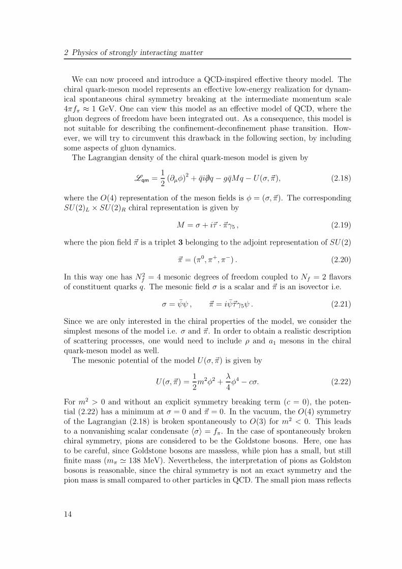
We can now proceed and introduce a QCD-inspired effective theory model. Thechiral quark-meson model represents an effective low-energy realization for dynam-ical spontaneous chiral symmetry breaking at the intermediate momentum scale4πfπ ≈ 1 GeV. One can view this model as an effective model of QCD, where thegluon degrees of freedom have been integrated out. As a consequence, this model isnot suitable for describing the confinement-deconfinement phase transition. How-ever, we will try to circumvent this drawback in the following section, by includingsome aspects of gluon dynamics.
The Lagrangian density of the chiral quark-meson model is given by
Lqm =1
2(∂µφ)2 + qi/∂q − gqMq − U(σ, ~π), (2.18)
where the O(4) representation of the meson fields is φ = (σ, ~π). The correspondingSU(2)L × SU(2)R chiral representation is given by
M = σ + i~τ · ~πγ5 , (2.19)
where the pion field ~π is a triplet 3 belonging to the adjoint representation of SU(2)
~π = (π0, π+, π−) . (2.20)
In this way one has N2f = 4 mesonic degrees of freedom coupled to Nf = 2 flavors
of constituent quarks q. The mesonic field σ is a scalar and ~π is an isovector i.e.
σ = ψψ , ~π = iψ~τγ5ψ . (2.21)
Since we are only interested in the chiral properties of the model, we consider thesimplest mesons of the model i.e. σ and ~π. In order to obtain a realistic descriptionof scattering processes, one would need to include ρ and a1 mesons in the chiralquark-meson model as well.
The mesonic potential of the model U(σ, ~π) is given by
U(σ, ~π) =1
2m2φ2 +
λ
4φ4 − cσ. (2.22)
For m2 > 0 and without an explicit symmetry breaking term (c = 0), the poten-tial (2.22) has a minimum at σ = 0 and ~π = 0. In the vacuum, the O(4) symmetryof the Lagrangian (2.18) is broken spontaneously to O(3) for m2 < 0. This leadsto a nonvanishing scalar condensate 〈σ〉 = fπ. In the case of spontaneously brokenchiral symmetry, pions are considered to be the Goldstone bosons. Here, one hasto be careful, since Goldstone bosons are massless, while pion has a small, but stillfinite mass (mπ ≃ 138 MeV). Nevertheless, the interpretation of pions as Goldstonbosons is reasonable, since the chiral symmetry is not an exact symmetry and thepion mass is small compared to other particles in QCD. The small pion mass reflects
14

2.3 The Polyakov quark-meson model
the explicit symmetry breaking through the two lightest quarks i.e. up and downquark.
Here we want to stress the fact that the scalar condensate is closely related tothe quark condensate 〈qq〉 and for small values of 〈σ〉 the two condensates areproportional in the chiral limit. At this point it is also interesting to emphasize thatchiral symmetry resembles a typical spin system known from statistical physics.
The explicit symmetry breaking term cσ in the potential provides the mass mπ
to the pions. At the tree level, the expression
c0 = fπm2π (2.23)
yields the physical pion mass in vacuum. For convenience we introduce a dimen-sionless parameter
h =c
c0(2.24)
as a measure for for the strength of the symmetry breaking term. The physical valueat tree level is h = 1. We will make use of this parameter later in Chapter 4. In amedium, the chiral symmetry of the Lagrangian is restored leading to a vanishingchiral condensate at some critical temperature and/or density.
Closely connected with the chiral quark-meson model are the following, very im-portant and useful relations. However, we refrain from going into details concerningtheir derivation and just quote them. The origin of their importance lies in thefact that knowing them, we can connect the parameters of the model with actualphysical observables. The first relation, that relates the constituent quark mass mq
to the pion decay constant fπ is the Goldberger-Treiman relation
gAmq = gfπ, (2.25)
where g is the Yukawa coupling and gA ≃ 1.25. In other words, this relation connectsthe minimum of the mesonic potential with fπ. On the other hand the Gell-Mann-Oakes-Renner relation is given by
m2πf
2π =
1
2(mu +md) 〈qq〉 = mc〈qq〉. (2.26)
Here we can relate the pion mass mπ to the chiral condensate 〈qq〉 and the currentquark mass mc.
2.3 The Polyakov quark-meson model
As we have already mentioned in the previous section, the chiral quark-meson modelis often used as an effective realization of the low-energy sector of QCD, whichbelongs to the O(4) universality class. It should however be emphasized that the low
15
2 Physics of strongly interacting matter
energy properties of QCD are captured only incompletely since confinement effectsare not properly taken into account. Clearly, any description of the QCD chiral phasetransition within the quark-meson model also has some drawbacks and limitations.Furthermore, due to the replacement of the local SU(Nc) gauge invariance by aglobal symmetry one can not address the deconfinement phenomena in QCD. Thelack of understanding the deconfinement phenomena is one of the most importantissues encountered in such an analysis. One possibility to circumvent this problemis to incorporate gluons and their dynamics into the existing chiral model. By doingso, confinement effects can be included, at least approximately. The importance ofincluding gluons is obvious, since their contribution to the bulk thermodynamics ofhot and dense matter is significant, as we will show in Chapter 5. Thus, the needfor having an appropriate model where gluonic degrees of freedom are included isobvious.
Before we give a closer description of the model itself, let us briefly and schemat-ically address the issue of confinement. Mesons and baryons represent the wellknown and at the same time the most observed states in nature. On a more ele-mentary level they consist of either quark/antiquark pair (mesons) or three quarks(baryons)6. The quarks interact via the exchange of gluons. Due to this interactionquarks/antiquarks are bound, i.e. confined, and thus not observed as free particles.In other words, quarks and gluons appear as free particles only at small distances.As a consequence, quarks can only be studied as constituents of hadrons.
Now we proceed with the question how one can address, and later incorporate insome given effective model, the effect of confinement. Here we follow the argumentsgiven in Refs. [13, 14]. An SU(N) non-Abelian gauge theory (with quarks included),as we have seen previously, is invariant under local SU(N) symmetry transformation.This implies that the covariant derivative (2.5) and field ψ transform as
Dµ → U †Dµ U , ψ → U † ψ , (2.27)
where the symmetry transformation U ∈ SU(N). However, one can define anothersymmetry transformation of the form
Uc = eiϑ I , (2.28)
where I represents the unit matrix. On the other hand, Uc belongs to the SU(N)group, hence it satisfies
detUc = 1, U †c Uc = Uc U †
c = I . (2.29)
From this requirement, one deduces that the phase factor in Eq. (2.28) must read
ϑ =2πn
N, n = 0, 1, . . . (N − 1) . (2.30)
6The most prominent baryons are proton (2 up and 1 down quark) and neutron (2 down and 1up quark).
16

2.3 The Polyakov quark-meson model
Figure 2.2: An artist’s view of confinement [5]. In nature there are no free quarksand any attempt to separate a pair of quarks will result in the productionof quark-antiquark pairs, yielding again color neutral objects, hadrons.
Thus, this symmetry transformation is not a continuous one, and hence it defines aglobal Z(N) symmetry transformation.
In a general case of an SU(N) non-Abelian gauge theory at finite temperature,Polyakov and ’t Hooft [12, 13] conjectured that there is a gauge invariant operatorthat can be identified as an order parameter. In the case of three colors (Nc = 3)the corresponding global symmetry transformations belong to the Z(3) group. Thisgroup is the center group of SUc(3) and from the mathematical point of view it isa cyclic group. The order parameter for the Z(3) symmetry group is constructedusing the Polyakov loop 7. The Polyakov loop represents one of the most importantobservables in QCD at finite temperatures. It is represented as a matrix in colorspace given by:
L(~x) = P exp
i
β∫
0
dτA0(~x, τ)
, (2.31)
where P stands for path ordering and β = 1/T . In the heavy quark limit the decon-finement phase transition is well defined and QCD has the Z(3) center symmetrywhich is spontaneously broken in the high temperature phase. The order parameter
7Some authors introduce an order parameter for the Z(N) symmetry via the so-called thermalWilson line. The Polyakov loop is then defined as a trace of the timelike Wilson line.
17

2 Physics of strongly interacting matter
of the Z(3) symmetry in this case is the thermal expectation value of the trace ofthe Polyakov loop
ℓ =1
Nc〈TrcL(~x)〉, ℓ∗ =
1
Nc〈TrcL
†(~x)〉. (2.32)
Under a global Z(3) transformation ℓ transforms by an overall phase factor
ℓ→ exp
(2πin
3
)
ℓ, n = 0, 1, 2. (2.33)
In the absence of dynamical quarks, i.e. in the heavy quark limit of QCD, theexpectation value of the Polyakov loop indeed serves as an order parameter for thedeconfinement phase transition. As a consequence of the confinement/deconfinementphase transition, the Polyakov loop acquires a nonzero expectation value. Thus, wehave
ℓ = 0 −→ confined phase (T < Td)
ℓ 6= 0 −→ deconfined phase (T > Td),
where Td is the deconfinement temperature. It is interesting to note that, contraryto the O(4) symmetry, the Z(3) symmetry is broken at high and not at low tem-peratures. Thus, in contrast to other symmetry breaking phase transitions, thehigh temperature phase is the ordered phase and consequently, the low temperaturephase the disordered one in the Z(3) symmetry.
In general, the fields ℓ and ℓ∗ are different at non-zero quark chemical potential.For the SUc(3) color gauge group the Polyakov loop matrix L satisfies the followingrules
LL† = 1 and detL = 1, (2.34)
and can be written in diagonal form
L = diag(
eiϕ, eiϕ′
, e−i(ϕ+ϕ′))
(2.35)
in the Polyakov gauge.It should be noted that in the presence of dynamical quarks the Z(3) symmetry
is explicitly broken and there is no order parameter which characterizes the decon-finement phase transition in this case. Nevertheless, the Polyakov loop remains auseful concept also for dynamical quarks, an indicator of a rapid crossover transitiontowards confinement.
The Polyakov quark-meson model was first introduced in Ref. [33] as a new methodto extend the 2-flavor chiral quark-meson model by coupling it with the Polyakovloop. In this model, it is possible to address both, the chiral and confining propertiesof QCD and investigate them on a mean field level.
18

2.3 The Polyakov quark-meson model
The Lagrangian of the PQM model is given by
Lpqm = q (i /D − g(σ + iγ5~τ~π)) q +1
2(∂µσ)2 +
1
2(∂µ~π)2 − U(σ, ~π) − U(ℓ, ℓ∗) , (2.36)
where U(ℓ, ℓ∗) is the potential for the gluon field expressed in terms of the tracedPolyakov loop and its conjugate. As in the case for the chiral quark-meson model,meson fields have an O(4) symmetry and the corresponding SU(2)L × SU(2)R rep-resentation given by φ = (σ, ~π) and σ + i~τ · ~πγ5 respectively. Thus, again one hasN2f = 4 mesonic degrees of freedom coupled to Nf = 2 flavors of constituent quarks
q. The coupling between the effective gluon field and the quarks is implementedthrough a covariant derivative
Dµ = ∂µ − iAµ, (2.37)
where the spatial components of the gauge field are set to zero i.e. Aµ = δµ0A0. Thepurely mesonic potential U(σ, ~π) of the model is defined as
U(σ, ~π) =λ
4
(σ2 + ~π2 − v2
)2 − cσ (2.38)
and the potential of the gluon field is given in the following form
U(ℓ, ℓ∗)
T 4= −b2(T )
2ℓ∗ℓ− b3
6(ℓ3 + ℓ∗3) +
b44
(ℓ∗ℓ)2 , (2.39)
with
b2(T ) = a0 + a1
(T0
T
)
+ a2
(T0
T
)2
+ a3
(T0
T
)3
(2.40)
where a0 = 6.75, a1 = −1.95, a2 = 2.625, a3 = −7.44, b3 = 0.75 and b4 = 7.5.The coefficients are chosen in such a way as to reproduce the equation of state inpure gauge theory on the lattice. At the temperature T0 = 270 MeV, which is thecritical temperature obtained for pure gauge theory, the potential (2.39) yields afirst order phase transition. However, the choice of the potential for the gluon fieldgiven by Eq. (2.39) is not the only one. Another possibility is to replace the higherorder polynomial terms in ℓ and ℓ∗ with a logarithmic term [24]. Thus, the potentialU(ℓ, ℓ∗) can be also expressed in the following form [58]
U(ℓ, ℓ∗)
T 4= −1
2a(T )ℓ∗ℓ+ b(T ) log
(1 − 6ℓ∗ℓ+ 4(ℓ3 + ℓ∗3) − 3(ℓ∗ℓ)2
), (2.41)
where
a(T ) = a0 + a1
(T0
T
)
+ a2
(T0
T
)2
, b(T ) = b3
(T0
T
)3
. (2.42)
19

2 Physics of strongly interacting matter
The coefficients (a0, a1, a2, b3) have different numerical values then the coefficientsin Eqs. (2.39) and (2.40).
The effective potential U(ℓ, ℓ∗) is constructed from lattice data and is required tosatisfy the Z(3) center symmetry like the pure gauge theory. Furthermore, in thepure gauge theory the mean value ℓ, ℓ∗ are given by the minima of U(ℓ, ℓ∗). Thus, atlow temperatures the effective Polyakov loop potential must have an absolute min-imum at ℓ = 0 in order to be consistent with lattice predictions. For temperaturesabove the critical one the minimum is shifted to some finite value of ℓ. Finally, athigh temperatures i.e. in the limit T → ∞ the value of the Polyakov loop is ℓ→ 1.
We will finish this chapter with a few remarks. We have briefly discussed thestrong interaction and some low-energy effective realization of it. We confined our-selves to the two-flavor model, knowing that QCD exhibits an approximate chiralsymmetry in the up/down sector (Nf = 2) and, that QCD in this sector then belongto the same universality class as the O(4) model. This particular feature we use inChapter 4. Furthermore, we do not attempt to incorporate all effects of the confine-ment in the effective model. Rather, we combine a chirally symmetric model withthe Polyakov loop potential constructed (with appropriately fitted parameters) soas to simulate the first order confinement/deconfinement phase transition. In Chap-ter 5 we present results which provide input for further theoretical/phenomenologicalstudies in this direction.
20

Chapter 3
Renormalization group method
The Renormalization Group (RG) is a theoretical tool, which among many otheravailable methods in physics, is considered to be one of the most important ideas inquantum field theory (QFT). Besides the RG there is a variety of other methods de-veloped over the years one uses to tackle various problems encountered in QFT, suchas perturbation theory or various numerical techniques. Although their usefulnessin solving and understanding a large number of problems has been demonstrated, itoften happens that the applicability of a particular method is restricted to a specificenergy or length scale. Moreover, many problems cannot be investigated due theapproximations used within these methods. Hence, there was a need for a methodthat, at least to some extent, overcomes all these problems. During the recent yearsthe RG method has proven to be one of the most promising tools theorists haveat hand. The applicability of RG covers a whole range of physics and physicalphenomena that are usually plagued with divergences. Starting with its role as anovel method in QFT, the RG has developed into an uniquely effective techniquewidely used also in statistical physics, condensed matter theory and all other areasof physics where non-perturbative effects make systematic calculations difficult.
One of the most successful application of the RG has been to the theory of phasetransitions and critical phenomena. Being in its nature highly non-perturbative,the critical phenomena turned out to be an ideal testing ground for the applicabilityof the RG method. In the vicinity of a second-order phase transition long rangefluctuations are important and have to be accounted for in the calculations. Also, atthe critical temperature Tc measurable physical observables diverge and a specific setof parmeters called critical exponents describe their behavior. Various experimentalobservations indicate that the critical exponents are universal and depend only onthe symmetry and dimension of the physical system under investigation. In thelight of these findings, one can understand the large amount of effort invested in
21

3 Renormalization group method
understanding the nature and origin of the singular behavior of thermodynamicfunctions at the critical point characterized by the critical exponents. For a long timethere has been only one theoretical approach for describing phase transitions knownas mean field approximation. Introduced by P. E. Weiss as a theory of magnetism,the mean field approximation where no fluctuations are taken into account, in manycases fails in giving an accurate and quantitatively correct description of phasetransitions. Also the values for critical exponents calculated within this simpleapproximation often differ significantly from their known experimental values sincemean field approximation neglects the influence of the fluctuations and other non-perturbative effects in the very vicinity of the phase transition. However, despiteall drawbacks, the mean field approximation has been applied as a testing tool toinvestigate a new type of phase transition. The important theoretical breaktrough inunderstanding the physics behind critical phenomena (and other non-perturbativephenomena) came with Wilson’s RG concept.
Wilson’s idea is based on a simple and yet very shrewd observation that onecan construct an effective theory for a specific set of degrees of freedom of somegiven physical system. This particular effective theory is constructed by integratingout degrees of freedom we are not interested in. Consequently we are left with asubset of the initial system where the original number of degrees of freedom hasbeen reduced. The core of Wilson’s idea is the procedure of coarse-graining. Withinsuch an approach, Wilson conjectured that it should be possible to integrate outirrelevant degrees of freedom (short distance quantities or the “high energy modes”)by an iterative procedure and in the limit of very small momenta (long distances) allrelevant physical information should then be contained in the effective Hamiltonian.
On the other hand, in 1966 Kadanoff introduced a technique called block spintransformation. This approach is also often used to elucidate the RG idea. Again,one reduces the degrees of freedom of a model, now given as Ising spins located on asquare lattice. The RG transformation is achieved through dividing the lattice intoblocks with the same length. We assume that each block contains four spins locatedat every corner. The procedure of reduction of degrees of freedom is done assumingthat four spins in one block can be treated as one single effective spin so that theoriginal lattice can be replaced with a new one.
The whole idea concerning the RG transformation is based on one simple, butessential fact that physics is scale dependent. In other words, there is a minimumlength a which one uses in describing a given set of physical phenomena. Differentdegrees of freedom as well as different dynamics reveal at each scale a. Thus, thereis a whole set of physical theories used to investigate the properties and behavior ofrelevant degrees of freedom at a given scale. At scales a ∼ 1 m, classical mechanicsplays a crucial role in describing and explaining physical phenomena. By furtherlowering the scale a, other relevant degrees of freedom will emerge such as nucleonsat scales a ∼ 10−13 cm or quarks at a ∼ (10−14 − 10−18) cm, for instance. Now itbecomes clear why it is possible to apply this important and indispensable technique
22

of successively integrating out certain (irrelevant) degrees of freedom from a physicaltheory. Altough at first sight this procedure might look a bit unphysical or evenillogical because of a possible lost of information, its core idea lies in the fact thattheories at one scale decouple from theories valid at another scale. It might wellbe that at Planck length scales (length of approximately 10−35 m) the (super)stringtheory is relevant, but in order to describe the motion of a pendulum we do notneed any knowledge about molecules, atoms, quarks or (super)strings.
One of the most significant advantages of the RG method is that it can describephysics across different momentum scales. In particular, within the RG frameworkone can capture the dynamics of the long-range fluctuations near the critical point.It should also be noted that in perturbation theory fluctuations of all wavelengthsare treated on the same footing. Here, within the RG approach one can choosean appropriate approximation scheme and do all necessary summations within thechosen scheme.
From the mathematical point of view the RG can be thought of as a set of sym-metry transformations that leave the physics invariant. Whenever there is someoperation (in this case a binary one) that has a specific set of features one can speakof a group1. However, altough the RG is a continuous (or discrete) group of sym-metry transformations it is not a group in a strict mathematical sense but only asemigroup. For treating the RG as a group in the algebraic sense, one importantfeature is missing and that is the inverse property. Generally, an RG transformationis not invertible (at least not without a serious ambiguity) and hence it is not agroup.
The basic idea of the renormalization group and its important features are pre-sented in this chapter following the arguments given in Refs. [15, 16]. One of thepossible RG approaches, the Functional Renormalization Group (FRG), we intro-duce later in this chapter which we close with a derivation of the flow equation forthe effective average action. For a more detailed discussion regarding the origin andapplications of the RG method, we refer the interested reader to [15, 16, 17] andreferences therein.
1For a given binary operation ∗, a set G with elements A, B, C . . . ∈ G represents a group if thefollowing four properties are fulfilled
A, B ∈ G → A ∗ B ∈ G closure,
A, B, C ∈ G → (A ∗ B) ∗ C = A ∗ (B ∗ C) associativity,
∀A ∈ G → I ∗ A = A ∗ I = A identity,
∀A ∈ G, ∃A−1 ∈ G → A ∗ A−1 = A−1 ∗ A = I inverse.
23

3 Renormalization group method
3.1 Basic ideas of the renormalization group
Let us start with an infinitely dimensional space of Hamiltonians H or in other wordsa space of coupling constants ~G. Here ~G = (G1, G2, . . . ) stands for the strengthsof all possible couplings compatible with the symmetries of a system. Furthermore,we pick some Hamiltonian of a given physical system H[s, ~G] ∈ H. The set s that
together with coupling constants ~G characterizes the Hamiltonian, represents somemicroscopic variables (vectors, tensors, etc. that can be thought of as quantumfields in a quantum field theory or spins located on discrete lattice sites in statisticalphysics). Each of these constants defines a point in the space H. The renormalizationgroup transformation can now be defined by introducing an operator R that actson the Hamiltonian H[s, ~G] in the following way
RH[s, ~G] = H′[s′, ~G′]. (3.1)
What is achieved by this transformation is that the initial Hamiltonian H[s, ~G]
is transformed or renormalized in order to obtain a new Hamiltonian H′[s′, ~G′].Furthermore, the RG transformation operator R also reduces the number of degreesof freedom N to
N ′ = N/ad (3.2)
where d is the dimension of a system and a is some spatial rescaling factor.Now, depending on the problem we want to handle, we might be interested only
in the physics at long distances (compared to the rescaling factor a). We expecthowever that the characteristics of long wavelength fluctuations are independent ofthe microscopic details of a theory. Hence, the idea is to remove all irrelevant degreesof freedom from the theory.
Let us divide our original set of variables s into the following two subsets i.e.
s< = sN ′, (3.3a)
s> = s(N −N ′). (3.3b)
Since we are not interested in the variables s>, they will be removed from the problemby integrating them out. After doing so, what is left is an effective Hamiltonian ofthe original system Heff [s<, ~G<]. This Hamiltonian contains only the informationnecessary to compute the long wavelength properties of the system.
Here we want to stress the fact that the RG transformation does not by any meanschange the partition function of the system. This is an essential feature that RGtransformation has to satisfy in order to leave the “original” physics unchanged.Indeed, the partition function of the renormalized system can be written in thefollowing form∫
N ′
ds′eH′[s′, ~G′] =
∫
N ′
ds<eHeff [s<, ~G<] =
∫
N ′
ds<
∫
N−N ′
ds>eH[s<+s>, ~G<+ ~G>] =
∫
N
dseH[s, ~G],
(3.4)
24

3.1 Basic ideas of the renormalization group
where from the last equation follows the “original “ partition function of the system.The next step that has to be done is the rescaling of all spatial vectors i.e.
x′
= x/a (3.5)
for coordinates, andp
′
= p a , (3.6)
for momenta. Accordingly, the variables s also have to be rescaled by some rescalingfactor 2 b in order to preserve their fluctuation magnitude.
Let us repeat what has been done up to now. We have basically rescaled thevariables that the Hamiltonian H[s, ~G] depends on, and obtained the renormalized
Hamiltonian Heff [s<, ~G<] = H′[s′, ~G′] that retains all the original information of thesystem. This procedure can now be repeated using the renormalized HamiltonianH′[s′, ~G′] as the starting one i.e.
RH′[s′, ~G′] = H′′[s′′, ~G′′], RH′′[s′′, ~G′′] = H′′′[s′′′, ~G′′′], . . . (3.7)
An important question arises during this iteration procedure and that is the oneregarding the end of the procedure. In other words, how many times can we spatiallyrescale variable s? The RG transformation of rescaling and relabeling stops at a fixedpoint that is defined as
RH∗[s∗, ~G∗] = H∗[s∗, ~G∗]. (3.8)
Here we have that a point under some RG transformation maps onto itself, thus theiteration procedure ends.
Here we should stress the importance and show a few interesting features of a fixedpoint. In the vicinity of a fixed point the RG equation defined by the transformationlaw Eq. (3.1), can be linearized. To do so, first we write the Hamiltonian H[s, ~G]near a fixed point as
H[s, ~G] = H∗[s∗, ~G∗] + δH[s, ~G] (3.9)
where δH[s, ~G] is small. According to Eq. (3.1) and using the main characteristic ofthe RG transformation at the fixed point we have the following expression
R(
H∗[s∗, ~G∗] + δH[s, ~G])
= H∗[s∗, ~G∗] + RlinδH[s, ~G] = H∗[s∗, ~G∗] + δH′[s′, ~G′],
(3.10)
where Rlin is a linear operator where higher order terms O((δH[s, ~G])2) are ne-glected. The original RG transformation (or differential equation if we replace theoperator R with a corresponding differential operator) has been reduced to a linearproblem in the vicinity of a fixed point. This gives us the possibility to determinethe eigenvalues and eigenvectors of the linear operator Rlin. Thus, we may write
RlinδHk[s, ~G] = λk(a)δHk[s, ~G] (3.11)
2Depending on the type of the variable s one has to use different rescaling factors.
25

3 Renormalization group method
and solve the eigenvalue problem to obtain the corresponding eigenvalues λk(a)and eigenvectors (or “eigenoperators“) δHk. Consequently, one can represent the
Hamiltonian H[s, ~G] using the following general expansion
H[s, ~G] = H∗[s∗, ~G∗] +∑
k
lkδHk[s, ~G], (3.12)
where lk are expansion coefficients. At this point we can introduce the notion ofrelevance of operators δHk[s, ~G]. For λk > 0 the operator is relevant at the fixedpoint, for λk < 0 the operator is irrelevant and in the case where λk = 0 the operatoris considered to be marginal. One can also raise a question regarding the importanceof a fixed point. In order to obtain a fixed point solution of a given physical system wehave to solve Eq. (3.8). This equation can be an algebraic or a differential equation.In the case that Eq. (3.8) has only a trivial solution the corresponding system hasno interactions and this fixed point solution is known as the Gaussian fixed point.Needless to say, from a physical point of view, the most interesting solutions arethe non trivial ones, the so called Wilson-Fisher fixed points. These non trivialfixed points represent then critical states of a given system. How the system inthe critical state behaves, depends on the properties of the RG transformation. Ifsome system, described by Hamiltonian H[s1, ~G1] ∈ H, undergoes a second orderphase transition at some critical temperature Tc, the correlation length ξ diverges.Under the RG transformation R, Hamiltonian H[s1, ~G1] maps onto H[s2, ~G2], andagain ξ diverges. Now, one can define the critical surface in the space H as a setof Hamiltonians H[si, ~Gi], i = 1, 2, 3 . . . for which ξ → ∞. The critical surface isstable under RG transformations (3.1). Also, at the fixed point the physics is sameat all scales.
Intimately related with the notion of a fixed point of the RG transformationis the concept of universality. In the space of Hamiltonians H we have, from aphysical point of view a variety of systems (systems that differ significantly fromeach other by having different physical character) described by their corresponding
Hamiltonians H[s, ~G]. Universality reflects the feature that, altough some physicalsystems show different properties or behavior, they belong to the same universalityclass if attracted by the same fixed point. This expedient feature is often used inthe theory of critical phenomena. If two different physical systems belong to thesame universality class, a full description of the critical behavior of, let us say, thefirst system can be obtained by studying the second system. In this case one usuallysays that these two systems have the same asymptotic long wavelength physics andthus the same universal behavior. As a consequence we can literally reduce thecomplexity of a problem.
26

3.2 Functional renormalization group
3.2 Functional renormalization group
In this section we give a more detailed description of one particular RG method,namely the functional renormalization group (FRG). As the name indicates, this ap-proach is based on the functional method used in computation of various generatingfunctionals that contain all relevant information about some physical system. Thus,the FRG incorporates the basic idea of the RG transformation with the functionalapproach.
The FRG is an important tool for addressing nonperturbative problems withinthe quantum field theory. It is based on an infrared (IR) regularization with themomentum scale parameter k of the full propagator which turns the correspondingeffective action into a scale dependent functional Γk [36, 37, 38, 39, 40, 41]. Thismethod is just one of many other RG techniques presently available. Later in thissection, we will outline the basics of FRG approach and derive its main part i.e. theflow equation for the effective average action that we later use as the starting pointin our FRG based calculations.
3.2.1 Effective average action
Before we give the basic concepts of the FRG and derive the corresponding flowequation let us first introduce a few important objects that appear in quantum fieldtheory and statistical physics and which allow us to introduce the notion of theeffective average action.
The basic object in the context of quantum field theory is the generating functionalof the n-point correlation functions. This functional is given by the following pathintegral representation in the presence of an external field or source J(x) in thed-dimensional Euclidean space R
d
Z[J ] =
∫
Dχe−S[χ]+R
xχ(x)J(x), (3.13)
where χ(x) : Rd → R is a single-component real field variable. The classical action
S[χ] that governs its dynamics is related to the corresponding Lagrangian3 L of
3Here we will be somewhat lax, and refer to L as the Lagrangian and not the Lagrangian density.Usually, one introduces the action S as the time integral of the Lagrangian L by
S =
∫
dtL ,
where the Lagrangian L is given as the spatial integral of the Lagrangian density L
L =
∫
d3xL .
Consequently the integration over the space-time volume V = dtd3x of the system yields the
27

3 Renormalization group method
the system by
S[χ] =
∫
x
L ,
∫
x
≡∫
ddx (3.14)
and the usual Boltzmann factor is given by exp(−S[χ]). The functional integrationthat appears in the definition of the generating functional Z[J ] stands for the sumover all microscopic states. Consequently, the field χ(x) represents different physicalobservables such as spin, magnetization, mass field etc. The functional Z[J ] is alsoknown as the partition function in statistical physics and without an external sourceJ(x) reads
Z = Tre−H/T =∑
n
e−En/T , (3.15)
where trace represents an integration over all microscopic degrees of freedom presentin a system and En are eigenvalues of the Hamiltonian H . The partition functionZ can also be expressed in the following form
Z =∑
i
∫
dχi 〈χi|e−H/T |χi〉 , (3.16)
where the summation is to be performed over all states. By making an analyticalcontinuation to imaginary time (t→ −iτ) the partition function takes the form4
Z =
∫
Dχi (τ)e−SE (3.17)
and SE is the Euclidean action.Now we turn back to the source dependent partition function Z[J ]. Greens func-
tions generated by taking functional derivatives of the functional Z[J ] with respectto the source J are disconnected Greens functions. Using this kind of Greens func-tions is not very suitable since they do not contribute to the S-matrix. Thus, oneusually introduces a generating functional for the connected Greens functions as
W [J ] = lnZ[J ]. (3.18)
Now, by taking the functional derivatives of W [J ] with respect to the source J(x)we obtain the average density correlation
δW [J ]
δJ(x)= 〈χ(x)〉 = φ(x) (3.19)
action S
S =
∫
V
L .
4For details about the path integral formalism and imaginary time we refer the interested readerto Ref. [97].
28

3.2 Functional renormalization group
or the density-density correlation
δ2W [J ]
δJ(x)δJ(y)= 〈χ(x)χ(y)〉 − 〈χ(x)〉〈χ(y)〉. (3.20)
Finally, the effective action Γ[φ] is obtained by a Legendre transformation
Γ[φ] = −W [J ] +
∫
x
φ(x)J(x) , (3.21)
and represents the generating functional of the one-particle irreducible (1PI) corre-lation functions. For a given physical theory existing sources or external fields cannow be obtained through the effective action Γ[φ] i.e.
δΓ[φ]
δφ(x)= J(x). (3.22)
Furthermore, it is obvious from Eq. (3.22) that for vanishing external fields theequilibrium state of a theory is given by the minimum of Γ[φ]. In other wordsthe ground state of a theory is given by the minimum of the effective action. Itshould also be stressed that the second functional derivative of the effective actionis equivalent to the inverse propagator. Another essential feature of Γ[φ] is that fieldequations derived from it include all quantum effects and thus are exact.
The effective average action Γk that depends on a scale k represents a simplegeneralization of the standard effective action Γ[φ] acting as the generating func-tional of the one-particle irreducible (1PI) Green functions. The main objective isto start at some high UV scale Λ where the physics is described by some classicalaction S and then to successively integrate out quantum fluctuations by loweringthe scale k. In this way it is possible to calculate the generating functional for 1PIgraphs. A particular feature Γk incorporates is that only fluctuations with momentaq2 ≥ k2 are included whereas fluctuations with q2 ≤ k2 are suppressed. This can beachieved following the same line of reasoning as by constructing the effective actionΓ[φ] where we have introduced the generating functional of the n-point correlationfunctions Z[J ]. Hence, we can define the k dependent generating functional Zk[J ]as
Zk[J ] =
∫
Λ
Dχe−S[χ]+R
xχ(x)J(x)−∆Sk [χ]. (3.23)
Here we have included a new term ∆Sk[χ] that represents an infrared (IR) cutoffterm and reads in the momentum space
∆Sk[χ] =1
2
∫ddq
(2πd)χ∗(q)Rk(q)χ(q) (3.24)
29

3 Renormalization group method
where χ∗(q) = χ(−q). There are several conditions that the cutoff function Rk(q)has to fullfill. Generally, for the regulator is required the following
limq2/k2→0
Rk(q2) > 0. (3.25)
This important requirement makes the effective propagator (at vanishing field) finitein the IR limit q2 → 0, and no IR divergences appear in the presence of masslessmodes. Consequently, the regulator Rk acts as an IR regulator. The second property
limk2/q2→0
Rk(q2) = 0 (3.26)
ensures that Rk vanishes in the IR. In this way the regulator Rk(q) is removed in thephysical limit and we can obtain in the limit k → 0 the 1PI generating functional(Γ = limk→0 Γk). Finally, by the third condition
limk→Λ
Rk(q2) → ∞ (3.27)
the initial conditions at the UV scale Λ are recovered and the scale dependenteffective action Γk approaches the microscopic action S in the UV limit.
The above mentioned features that the IR cutoff has to satisfy can be implementedby the e.g. following form
Rk(q) ∼q2
eq2/k2 − 1. (3.28)
Generally, it is not always an easy task to find an adequate cutoff function. If thereare low mass fermions in a theory, the regulator must preserve chiral symmetry. Forgauge theories the situation is even worse owing to gauge symmetry breaking by theregulator. In our work we do not encounter these problems5. In our calculations weshall use the so called optimized cutoff functions for reasons which will be explainedin the forthcoming chapter. Their precise description will be given later in thissection.
The next logical step in the derivation of the effective average action is to definethe scale-dependent generating functional for the connected Greens functions by
Wk[J ] = lnZk[J ]. (3.29)
As in the case for the effective action Γ[φ] (cf. Eq. (3.19)) the expectation valuesof the fields χ in the presence of the cutoff term ∆Sk[χ] are obtained by taking thefunctional derivatives of Wk[J ] with respect to the source J(x). Finally, using amodified Legendre transformation of the form
Γk[φ] = −Wk[J ] +
∫
x
φ(x)J(x) − ∆Sk[φ] (3.30)
5The problem of gauge symmetry breaking in the presence of cutoff functions can be successfullycircumvented via modified Ward-Takahashi identities that recover the original gauge invariance.
30

3.2 Functional renormalization group
0 0.2 0.4 0.6 0.8 1
0.40.60.8
11.21.41.61.8
2
scale k
Γk
k=0 k=Λ
IR UV
Γ1PIS
Figure 3.1: Illustration of interpolation of the effective average action Γk betweenthe classical action S at some UV scale Λ and the full quantum actionΓ in the limit k → 0 in the IR.
we can define the effective average action Γk. The effective average action Γk governsthe dynamics of a theory at a momentum scale k and interpolates between the bareaction Γk=Λ ≡ S and the full quantum effective action Γk=0 = Γ. In Fig. 3.1 werepresent graphically this interpolation of Γk between S and Γk=0. At k = 0 there isno IR cutoff present anymore. Thus all fluctuations are included and by definitionthe effective average action equals the standard action (the generating functional of1PI Green functions). If there is some physical UV cutoff Λ in a theory the effectiveaverage action at the scale k = Λ Γk=Λ is associated with the microscopic (classical)action S.
3.2.2 Flow equation
Now we will derive the flow equation for the effective average action. This flowequation is essential and represents the crucial part in the FRG approach. Usingthis particular flow equation, we are able to follow the change of the scale dependenteffective action Γk at scale k with a change of the RG scale.
For the sake of simplicity we will consider only a one component field φ (e.g.scalar theory). First, we take a derivative of Eq. (3.30) with respect to the scale k
∂kΓk[φ] = −∂kWk[J ] −∫
x
δWk
δJ(x)∂kJ(x) +
∫
x
φ(x)∂kJ(x) − ∂k∆Sk[φ]. (3.31)
According to Eq. (3.19) the second and third term cancel. Furthermore, it follows
31

3 Renormalization group method
Figure 3.2: A typical cutoff function Rk and its derivative ∂tRk in the FRG approachas a functions of momentum p2. Both functions are shown for fixedk2 [40].
from Eq. (3.24) that the derivative of the cutoff term ∆Sk[φ] is of the form
∂k∆Sk[φ] =1
2
∫
x,y
φ(x)∂kRkφ(y). (3.32)
In order to proceed with the derivation, we first have to find the scale derivative ofthe scale-dependent generating functional for the connected Greens functions Wk[J ]for a fixed source J . Thus, starting from Eq. (3.29) we have
∂kWk[J ] =1
Zk∂k
∫
Dχe−S[χ]+R
xχ(x)J(x)−∆Sk [χ]
=1
Zk
∫
Dχ (−∂k∆Sk[χ]) e−S[χ]+R
xχ(x)J(x)−∆Sk [χ]
=1
Zk
∫
Dχ
−1
2
∫
x,y
χ(x)∂kRkχ(y)
e−S[χ]+R
xχ(x)J(x)−∆Sk [χ]
= −1
2
∫
x,y
∂kRk1
Zk
∫
Dχχ(x)χ(y)e−S[χ]+R
xχ(x)J(x)−∆Sk[χ]
︸ ︷︷ ︸
〈χ(x)χ(y)〉
. (3.33)
Now, we can use Eq. (3.19) and Eq. (3.20) to write the following decomposition
〈χ(x)χ(y)〉 = G(x, y) + φ(x)φ(y), (3.34)
32

3.2 Functional renormalization group
where we have introduced the notation
G(x, y) =δ2W [J ]
δJ(x)δJ(y)(3.35)
for the connected two-point functions. Plugging this result into Eq. (3.31) we endup with the flow equation for the effective average action
∂kΓk[φ] =1
2
∫
x,y
G(x, y)∂kRk. (3.36)
Altough we have derived the flow equation for Γk[φ] we will go one step further andexpress this flow as a functional differential equation for the effective average actionΓk[φ].
In order to do so let us first find the inverse of G(x, y). The starting point isEq. (3.30) and its variation with respect to the field φ(x). Thus, using the variationcondition on the effective average action we have
δΓk[φ]
δφ(x)= −δWk[J ]
δφ(x)+
∫
y
δJ(y)
δφ(x)φ(y) +
∫
y
J(y)δ(x− y) − δ∆Sk[φ]
δφ(x)
= −∫
y
δWk[J ]
δJ(y)︸ ︷︷ ︸
φ(y)
δJ(y)
δφ(x)+
∫
y
δJ(y)
δφ(x)φ(y) + J(x) − δ∆Sk[φ]
δφ(x)
= J(x) − δ∆Sk[φ]
δφ(x)
= J(x) − φ(x)Rk. (3.37)
The variation of the cutoff term is obtained using Eq. (3.24), but now given incoordinate space
δ∆Sk[φ]
δφ(x)=
δ
δφ(x)
1
2
∫
y,z
φ(y)Rkφ(z)
= φ(x)Rk (3.38)
The second variation with respect to φ(y) gives
δ2Γk[φ]
δφ(x)δφ(y)=δJ(x)
δφ(y)−Rk(x, y), (3.39)
where we have introduced the short hand notation Rk(x, y) = Rkδ(x− y). The goalwe aim for is to show the following identity
δJ(x)
δφ(y)=
(δ2W
δJ(x)δJ(y)
)−1
. (3.40)
33

3 Renormalization group method
∂kΓk[φ] = 12
Figure 3.3: Graphical representation of the flow equation for the effective averageaction Γk[φ]. The complete field dependent propagator is represented bythe double line and the solid dot denotes the insertion of ∂kRk.
By taking a variation on Eq. (3.19) with respect to φ(y) we have
δ
δφ(y)
(δW [J ]
δJ(x)
)
= δ(x− y). (3.41)
Thus, we can write the following set of identities
δ(x− y) =δ2W
δJ(x)δφ(y)=
∫
z
(δ2W
δJ(x)δJ(z)
δJ(z)
δφ(y)
)
(z, y)
=
∫
z
δ2W
δJ(x)δJ(z)
(δ2Γk[φ]
δφ(z)δφ(y)+Rk
)
(z, y)
=
∫
z
δ2W
δJ(x)δJ(z)
(
Γ(2)k [φ] +Rk
)
(z, y). (3.42)
From the last step follows Eq. (3.40). Finally, we can write the flow equation forthe effective average action Γk[φ] as
∂kΓk[φ] =1
2
∫
x,y
G(x, y)∂kRk =1
2
∫
x
[(
Γ(2)k [φ] +Rk
)−1
∂kRk
]
. (3.43)
Since no approximations have been introduced during the derivation of flow equationfor the effective average action Γk[φ], this flow is in the literature also referred toas the exact RG flow equation. However, as one starts with the tedious procedureof solving the exact flow equation, various approximation schemes and truncationshave to be used and the exactness is lost.
The flow equation can be written in momentum space and extended to includefermions as well. The full form of the flow equation is usually written in the following
34

3.2 Functional renormalization group
more compact matrix form
∂kΓk[Φ, ψ, ψ] =1
2STr
[(
Γ(2)k [Φ, ψ, ψ] + Rk
)−1
∂kRk
]
(3.44)
where the matrix Γ(2)k [Φ, ψ, ψ] has the following block substructure in boson-antifermion-
fermion space
Γ(2)k [Φ, ψ, ψ] =
Γ(2)k,ΦΦ Γ
(2)
k,ΦψΓ
(2)k,Φψ
Γ(2)
k,ψΦΓ
(2)
k,ψψΓ
(2)
k,ψψ
Γ(2)k,ψΦ Γ
(2)
k,ψψΓ
(2)k,ψψ
, (3.45)
and the elements of matrix (3.45) are second order functional derivatives of Γk withrespect to corresponding fields. The supertrace STr in the Eq. (3.44) denotes amomentum integration and a summation over all internal indices like e.g. flavor,color, and/or Dirac indices and Φ and ψ, ψ denote bosonic and (anti)fermionic fields,respectively. The cutoff function has also an appropriate matrix structure
Rk =
RkB 0 00 0 RkF
0 −RkF 0
, (3.46)
where RkB denotes bosonic and RkF fermionic regulator. It should be noted thatthe IR cutoff does not mix bosons and fermions.
The flow equation for the effective average action is a functional differential equa-tion because of the appearance of the exact propagator (Γ
(2)k [φ] + Rk)
−1. Also, thebare action S enters the flow only in the form of an initial condition. A specificphysical system investigated within the FRG approach is completely defined viaEq. (3.44) and the initial condition ΓΛ = S. Together with a given form of thecutoff function Rk one has a closed system with no infinities in the flow equationand all microscopic physics is encoded in the microscopic effective action ΓΛ. Thereason why infinities are absent in the flow equation is because the term ∂kRk ispresent. Indeed, only momenta q2 ≤ k2 contribute to the flow at scale k i.e. thehigh momentum modes q2 ≥ k2 are effectively integrated out. As a consequence weare left with a completely finite flow, both in the UV and in the IR regime.
The flow equation has also a simple one loop structure as shown in Fig. 3.3.Contrary to the perturbation theory where n-loop diagrams require n dimensionalintegrals, here one has to deal with only one integral.
In the end, it is interesting to note a close resemblance of the flow equation (3.44)to a one-loop equation. Indeed, for the lowest non-trivial order of the loop expansionone obtains
Γk[φ] = S[φ] +1
2Tr log
(S(2)[φ] +Rk
). (3.47)
35
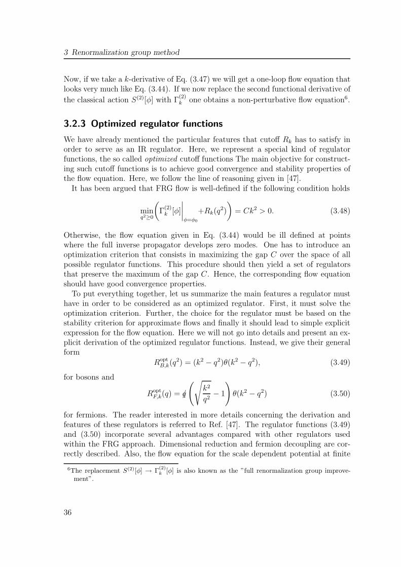
3 Renormalization group method
Now, if we take a k-derivative of Eq. (3.47) we will get a one-loop flow equation thatlooks very much like Eq. (3.44). If we now replace the second functional derivative of
the classical action S(2)[φ] with Γ(2)k one obtains a non-perturbative flow equation6.
3.2.3 Optimized regulator functions
We have already mentioned the particular features that cutoff Rk has to satisfy inorder to serve as an IR regulator. Here, we represent a special kind of regulatorfunctions, the so called optimized cutoff functions The main objective for construct-ing such cutoff functions is to achieve good convergence and stability properties ofthe flow equation. Here, we follow the line of reasoning given in [47].
It has been argued that FRG flow is well-defined if the following condition holds
minq2≥0
(
Γ(2)k [φ]
∣∣∣∣φ=φ0
+Rk(q2)
)
= Ck2 > 0. (3.48)
Otherwise, the flow equation given in Eq. (3.44) would be ill defined at pointswhere the full inverse propagator develops zero modes. One has to introduce anoptimization criterion that consists in maximizing the gap C over the space of allpossible regulator functions. This procedure should then yield a set of regulatorsthat preserve the maximum of the gap C. Hence, the corresponding flow equationshould have good convergence properties.
To put everything together, let us summarize the main features a regulator musthave in order to be considered as an optimized regulator. First, it must solve theoptimization criterion. Further, the choice for the regulator must be based on thestability criterion for approximate flows and finally it should lead to simple explicitexpression for the flow equation. Here we will not go into details and present an ex-plicit derivation of the optimized regulator functions. Instead, we give their generalform
RoptB,k(q
2) = (k2 − q2)θ(k2 − q2), (3.49)
for bosons and
RoptF,k(q) = q/
(√
k2
q2− 1
)
θ(k2 − q2) (3.50)
for fermions. The reader interested in more details concerning the derivation andfeatures of these regulators is referred to Ref. [47]. The regulator functions (3.49)and (3.50) incorporate several advantages compared with other regulators usedwithin the FRG approach. Dimensional reduction and fermion decoupling are cor-rectly described. Also, the flow equation for the scale dependent potential at finite
6The replacement S(2)[φ] → Γ(2)k [φ] is also known as the ”full renormalization group improve-
ment”.
36

3.2 Functional renormalization group
temperature and chemical potential that is derived using the set of optimized regu-lators, can be factorized into a thermal and vacuum part. Consequently, the thermaland vacuum part contribute additively to the flow. Numerical stability of the solu-tions of the flow equation is also achieved by using the regulators (3.49) and (3.50).
In the forthcoming chapter we will use the above mentioned regulators, slightlymodify them and adapt them to suit our needs in the case for finite temperaturesand chemical potential and in the presence of a gluonic background.
37

38

Chapter 4
Critical phenomena and O(4) scaling
The understanding of the phase structure and the critical properties of the stronglyinteracting medium is one of the central problems that is addressed in the contextof QCD. Lattice Gauge Theory (LGT) calculations show that at finite temperaturethere is a clear separation between the confined-hadronic and deconfined, quark-gluon plasma phase. Following universality arguments, it is expected, that two-flavorQCD exhibits the second order chiral phase transition and belongs to the same uni-versality class as the O(4) spin system in three dimensions [52, 53, 54, 55, 56, 57].Consequently, the long-range properties of the chiral phase transition can be studiedindependently of the specific dynamics within various effective models. The chiralquark-meson model is often used as an effective realization of the low-energy sectorof the QCD belonging to the O(4) universality class [66]. The concept of universal-ity allows us to study the chiral quark-meson model (or any other suitable effectivemodel that belongs to the same O(4) class) instead of QCD itself in order to extractinformation concerning the critical behavior. Thus, by exploring the thermody-namics near the phase transition within this model, one can unravel the leadingsingularities of thermodynamic quantities in two-flavor QCD at the second orderchiral phase transition. Clearly, any description of the QCD chiral phase transi-tion within the quark-meson model has some limitations. First, one cannot addressto the deconfinement phenomena in QCD and second, one cannot obtain quanti-tative information on the thermodynamics outside the chiral critical region or onnon-universal quantities like the critical temperature Tc. However, by exploring thethermodynamics of this model, we can study the problem of the universal propertiesrelated with the dynamical chiral symmetry breaking at finite temperature and/ordensity. In general, the phase transition and critical phenomena are connected witha singular behavior of various susceptibilities which are related to fluctuations ofphysical quantities. In a system with a second order phase transition there are long
39

4 Critical phenomena and O(4) scaling
range critical correlations that appear due to the presence of massless modes. Thisresults in divergent fluctuations.
The mean field theory, often used to describe the chiral phase transition [58,59, 42], usually fails to give a correct description of the critical phenomena sinceit neglects the influence of the fluctuations and non-perturbative effects near thephase transition. However, the methods based on the renormalization group (RG)can account for both these important effects (see eg. [17]). The advantage of theRG method is that it can describe physics across different momentum scales. Inparticular, within the RG framework one can capture the dynamics of the long-range fluctuations near the critical point. The Wilsonian RG techniques such as thefunctional renormalization group (FRG) are particularly useful in describing phasetransitions [39].
The phase transition in the chiral quark-meson model has already been studiedusing different RG approaches [60, 61, 62, 63, 64, 65, 66, 67] both in the vacuum aswell as in the medium at finite temperature and chemical potential. Also, variouscritical exponents at the critical point have also been calculated. One of the im-portant results of the RG theory is the prediction, that near the phase transition,the models belonging to the same universality class should have the same criticalexponents and the scaling functions.
In this chapter we study the universal properties of the chiral phase transitionwithin the FRG method applied to the chiral quark-meson model. Furthermore, wealso examine the scaling functions for different physical quantities and the equationof state. We obtain the critical exponents for the order parameter and its transverseand longitudinal susceptibilities as well as the correlation lengths and calculate theeffective critical exponents in the presence of a chiral symmetry breaking field. Fi-nally, we show a direct way for determining the critical exponents, and explore thescaling behavior of different ratios of the susceptibilities and the order parameter.We close this chapter by showing that within the FRG method and upon applicationof the suitable truncation of the FRG flow equation, the chiral quark-meson modelexhibits the universal behavior that is quantitatively consistent with that obtainedrecently in the LGT calculations for the O(4) spin system in three dimensions.
4.1 FRG method at finite temperature and chemical
potential
We start with the chiral quark-meson model in order to explore the scaling propertiesof the chiral phase transition and the corresponding critical equation of state. Thisparticular effective model is relevant for studying strongly interacting hot and densematter with two degenerate light-quark flavors, since it is expected to belong to thesame universality class as QCD at the chiral phase transition.
40

4.1 FRG method at finite temperature and chemical potential
We use the FRG method to explore the critical properties near the chiral phasetransition. The advantage we have of using this RG scheme is that we can obtaina quantitatively correct description of critical phenomena, since the influence offluctuations and non-perturbative effects are taken into account within this method.We are also able to find an effective potential at finite temperature and density.
We start with the flow equation (3.44) written in the form where bosonic andfermionic contributions to the flow are separated. Here we do not have fermionsources (constant fermionic background) so that Eq. (3.44) reduces to
∂kΓk[Φ, ψ] =1
2Tr
[(
Γ(2)k [Φ, ψ] +RkB
)−1
∂kRkB
]
−Tr
[(
Γ(2)k [Φ, ψ] +RkF
)−1
∂kRkF
]
,
(4.1)
where Γ(2)k denotes the second functional derivative of Γk[Φ, ψ] with respect to the
field variables and corresponds to the inverse exact propagator at the scale k. Theregulators RkB and RkF denote bosonic and fermionic cutoff functions respectively.Finally, the trace in Eq. (4.1) denotes a momentum integration and a summationover all internal indices like e.g. flavor, color, and/or Dirac indices.
The effect of fluctuations, which is of crucial importance if we want to obtaina correct picture of chiral phase transition, is gradually included in Γk by solvingthe FRG flow equation (4.1). This procedure corresponds to solving an infinitetower of coupled functional differential equations. Needless to say, such a demandposes an unavailing task. Thus, in practice one has to find a suitable truncation ofthis system of equations and a corresponding approximation to the effective averageaction. Here, we employ the following truncation for the effective action given inEuclidean space-time
Γk =
∫
d4x
[1
2Zφ,k (∂µφ)2 + Zψ,kψ∂/ψ + gψ (σ + i~τ · ~πγ5)ψ + Uk(ρ)
]
, (4.2)
where the field ρ is introduced as
ρ =1
2φ2 =
1
2
(σ2 + ~π2
), φ = (σ, ~π). (4.3)
and the fermionic field ψ carries two flavors corresponding to the up and downquarks.
In the following we assume that each spectral function is dominated by a pole,corresponding to a quasiparticle. Furthermore, we neglect the wavefunction renor-malization for both the bosonic and fermionic fields (Zφ,k = Zψ,k = 1), i.e. theanomalous dimension is set to zero. Thus, changes of quasiparticle properties inthe medium are accounted for, but the fragmentation of single-particle strengthis ignored. Finally, we neglect the scale dependence of the Yukawa coupling g inEq. (4.2). Consequently, the only scale dependence we are left with is that of the
41
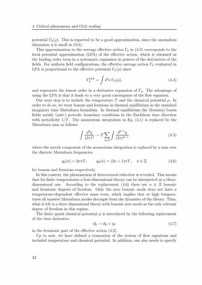
4 Critical phenomena and O(4) scaling
potential Uk(ρ). This is expected to be a good approximation, since the anomalousdimension η is small in O(4).
This approximation to the average effective action Γk in (4.2) corresponds to thelocal potential approximation (LPA) of the effective action, which is obtained asthe leading order term in a systematic expansion in powers of the derivatives of thefields. For uniform field configurations, the effective average action Γk evaluated inLPA is proportional to the effective potential Uk(ρ) since
ΓLPAk =
∫
d4xUk(ρ), (4.4)
and represents the lowest order in a derivative expansion of Γk. The advantage ofusing the LPA is that it leads to a very good convergence of the flow equation.
Our next step is to include the temperature T and the chemical potential µ. Inorder to do so, we treat bosons and fermions in thermal equilibrium in the standardimaginary time Matsubara formalism. In thermal equilibrium the (fermion) bosonfields satisfy (anti-) periodic boundary conditions in the Euclidean time directionwith periodicity 1/T . The momentum integration in Eq. (4.1) is replaced by theMatsubara sum as follows:
∫ddq
(2π)d→ T
∑
n∈Z
∫dd−1q
(2π)d−1(4.5)
where the zeroth component of the momentum integration is replaced by a sum overthe discrete Matsubara frequencies
q0(n) = 2nπT, q0(n) = (2n+ 1)πT , n ∈ Z (4.6)
for bosons and fermions respectively.In this context, the phenomenon of dimensional reduction is revealed. This means
that for finite temperatures a four-dimensional theory can be interpreted as a three-dimensional one. According to the replacement (4.6) there are n ∈ Z bosonicand fermionic degrees of freedom. Only the zero bosonic mode does not have atemperature-dependent effective mass term, which implies that at high tempera-tures all massive Matsubara modes decouple from the dynamics of the theory. Thus,what is left is a three dimensional theory with bosonic zero mode as the only relevantdegree of freedom in this regime.
The finite quark chemical potential µ is introduced by the following replacementof the time derivative
∂0 → ∂0 + iµ (4.7)
in the fermionic part of the effective action (4.2).Up to now, we have defined a truncation of the system of flow equations and
included temperature and chemical potential. In addition, one also needs to specify
42

4.1 FRG method at finite temperature and chemical potential
the regulator functions Rk. As we have already mentioned in the previous chap-ter, we will use the optimized cutoff functions throughout this work. However, weemploy a slightly modified form of the optimized regulator, where the Euclidean4-momentum squared q2 is replaced by the 3-momentum squared q2. Thus, as abosonic regulator function we use the following choice
RoptB,k(q
2) = (k2 − q2)θ(k2 − q2). (4.8)
The fermionic cutoff function should be consistent with chiral symmetries of thesystem under investigation. One possibility to preserve this consistency is to requirethe same Lorentz structure for the fermionic regulator RkF as for the kinetic termfor free fermions. At finite chemical potential µ we use [48]
RoptF,k(q) =
(q/+ iµγ0
)
(√
(q0 + iµ)2 + k2
(q0 + iµ)2 + q2− 1
)
θ(k2 − q2). (4.9)
Clearly, the modified regulator functions are invariant only under spatial rotationsof the momentum q in a particular frame, but not under Euclidean rotations involv-ing the imaginary time direction. However, this is not a crucial issue in calculationsat finite temperature and chemical potential, where the heath bath anyway definesa preferred frame. Furthermore, the Euclidean invariant form leads to various diffi-culties, as pointed out in [68]. A great advantage of the regulators (4.8) and (4.9)is that in the quasiparticle approximation, the Matsubara sums for the one loopdiagrams are identical to those appearing in a free theory.
Let us now derive the flow equation for the effective average action at finite Tand µ with the above generalization. First, we note that one can separate thecontributions from bosonic and fermionic fluctuations, respectively
∂kUk(ρ) = ∂kUk,B(ρ) + ∂kUk,F (ρ). (4.10)
We start the derivation by considering only the bosonic part of the flow in thevacuum and include temperature later.
Within the LPA, the bosonic part of the flow is given by the following expressionin momentum space
∂kUk,B(ρ) =1
2Tr
[(∂2Uk(ρ)
∂φi∂φj+ (q2 +RkB)δij
)−1
∂kRkB
]
. (4.11)
Further, according to Eq. (4.3) the derivatives of the effective potential are
∂Uk(ρ)
∂φi=∂Uk(ρ)
∂ρ
∂
∂φi
(1
2φnφn
)
=∂Uk(ρ)
∂ρφnδin (4.12)
43
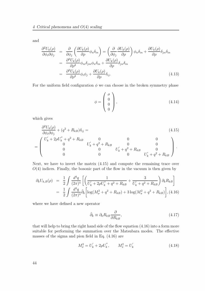
4 Critical phenomena and O(4) scaling
and
∂2Uk(ρ)
∂φi∂φj=
∂
∂φj
(∂Uk(ρ)
∂ρφnδin
)
=
(∂
∂φj
∂Uk(ρ)
∂ρ
)
φnδin +∂Uk(ρ)
∂ρδjnδin
=∂2Uk(ρ)
∂ρ2φmδjmφnδin +
∂Uk(ρ)
∂ρδjnδin
=∂2Uk(ρ)
∂ρ2φiφj +
∂Uk(ρ)
∂ρδij . (4.13)
For the uniform field configuration φ we can choose in the broken symmetry phase
φ =
σ000
, (4.14)
which gives
∂2Uk(ρ)
∂φi∂φj+ (q2 +RkB)δij = (4.15)
=
U′
k + 2ρU′′
k + q2 +RkB 0 0 00 U
′
k + q2 +RkB 0 00 0 U
′
k + q2 +RkB 00 0 0 U
′
k + q2 +RkB
.
Next, we have to invert the matrix (4.15) and compute the remaining trace overO(4) indices. Finally, the bosonic part of the flow in the vacuum is then given by
∂kUk,B(ρ) =1
2
∫d4q
(2π)4
[(1
U′
k + 2ρU′′
k + q2 +RkB
+3
U′
k + q2 +RkB
)
∂kRkB
]
=1
2
∫d4q
(2π)4∂k
[
log(M2σ + q2 +RkB) + 3 log(M2
π + q2 +RkB)
]
, (4.16)
where we have defined a new operator
∂k ≡ ∂kRkB∂
∂RkB, (4.17)
that will help to bring the right hand side of the flow equation (4.16) into a form moresuitable for performing the summation over the Matsubara modes. The effectivemasses of the sigma and pion field in Eq. (4.16) are
M2σ = U
′
k + 2ρU′′
k , M2π = U
′
k (4.18)
44

4.1 FRG method at finite temperature and chemical potential
where the primes denote derivatives with respect to the field ρ. Evaluated at thevacuum expectation value the masses reduce to the physical masses at the scalek = 0.
Now, in the bosonic part of the vacuum flow (4.16) we can include a temperatureT via Eq. (4.5) (q0 = q0(n) = 2nπT ) and make use of the optimized bosonic regula-tor (4.8). Being now in a heath bath, we can switch our notation, and use, insteadof the k-dependent effective potential Uk(ρ) a scale dependent grand canonical po-tential Ωk(T, µ; ρ). In the LPA, the effective average action Γk is proportional tothe effective potential (cf. Eq. (4.4)) and generally, the effective action Γ can beexpressed in terms of the effective potential (i.e. the grand canonical potential) as
Ω =T
VΓ . (4.19)
Thus, for the bosonic contribution we have the following
∂kΩk,B(T, µ; ρ) =1
2
∫d3q
(2π)3T
+∞∑
n=−∞
∂
∂k
[log(q2
0 + q2 +M2σ + k2 − q2)
+ 3 log(q20 + q2 +M2
π + k2 − q2)]. (4.20)
Due to the form of the optimized cutoff function, the momentum integration istrivial to perform, thus we are left only with the following sum over the Matsubaramodes
∂kΩk,B(T, µ; ρ) =k4
6π2T
+∞∑
n=−∞
(1
q20 + E2
σ
+3
q20 + E2
π
)
(4.21)
whereEσ =
√
k2 +M2σ , Eπ =
√
k2 +M2π (4.22)
denote the sigma and pion energies, respectively. Finally, using the standard results,we can perform the Matsubara summation as follows
+∞∑
n=−∞
(1
q20 + ω2
)
=1
2Tωcoth
( ω
2T
)
. (4.23)
Let us now turn to the fermionic part of the flow that can be written in thefollowing form
∂kUk,F (ρ) = −Tr[(
Γ2k +RkF
)−1∂kRkF
]
, (4.24)
where the functional derivatives of Γk with respect to the fields ψ and ψ have to betaken in the fermion-antifermion space and read
Γ2k[ψ, ψ] = q/+ iµγ0 + g(σ + i~τ · ~πγ5). (4.25)
45

4 Critical phenomena and O(4) scaling
The trace in the fermion-antifermion space represents now both, momentum inte-gration and summation over flavor, color, and Dirac indices. Defining the fermionicanalogue of the operator (4.17), summing over internal indices and using the identityTr log = log det we have1
∂kUk,F (ρ) = −νq∫
d4q
(2π)4
∂
∂klog det
[
q/+ iµγ0 + g(σ + i~τ · ~πγ) +RkF
]
. (4.26)
With νq = 2NcNf = 12 we have denoted the number of internal quark degrees offreedom. After calculating the determinant in (4.26) one obtains
∂kUk,F (ρ) = −νq∫
d4q
(2π)4
∂
∂klog
(
(q0 + iµ)2 + k2 +M2q
)
, (4.27)
where Mq is the effective quark mass
M2q = 2ρg2. (4.28)
Inclusion of temperature in (4.27) and calculation of the momentum integral (thisis again trivial, due to the optimized fermionic cutoff function (4.9)) leads to thefollowing expression for the fermionic contribution to the flow of k-dependent grandcanonical potential
∂kΩk,F (T, µ; ρ) = −2νqk4
6π2T
n=+∞∑
n=−∞
1
(q0 + iµ)2 + E2q
, (4.29)
where we now have q0 = q0(n) = (2n+ 1)πT and the quark energy given by
Eq =√
k2 + 2ρg2. (4.30)
The sum appearing in Eq. (4.29) has to be slightly rearranged in order to performMatsubara summation. A simple algebraic manipulation yields
∑
n
1
(q0 + iµ)2 + E2q
=1
2Eq
∑
n
(Eq − µ
q20 + (Eq − µ)2
+Eq + µ
q20 + (Eq + µ)2
)
. (4.31)
Finally, using again standard techniques, the Matsubara summation can be per-formed with the following result
+∞∑
n=−∞
(1
q20 + ω2
)
=1
2Tωtanh
( ω
2T
)
. (4.32)
1Here we deal with a determinant of 2 × Nc × Nf = 12 dimensional matrix in Dirac, color andflavor space.
46

4.1 FRG method at finite temperature and chemical potential
Now we can put all the pieces together and write down the flow equation for thescale dependent grand canonical potential Ωk(T, µ) within the FRG approach forthe chiral quark-meson model
∂kΩk(T, µ; ρ) =k4
12π2
[3
Eπcoth
(Eπ2T
)
+1
Eσcoth
(Eσ2T
)
− νq1
Eq
(
tanh
(Eq − µ
2T
)
+ tanh
(Eq + µ
2T
))]
. (4.33)
By rewriting Eq. (4.33) by means of occupation numbers, we obtain a more trans-parent form of the flow equation [48]
∂kΩk(T, µ; ρ) =k4
12π2
[
3
Eπ
(
1 + 2nB(Eπ)
)
+1
Eσ
(
1 + 2nB(Eσ)
)
− 2νqEq
(
1 − nF (Eq) − nF (Eq)
)]
. (4.34)
Here nB(Eπ,σ) and nF (Eq), nF (Eq) represent the well known bosonic and fermionicdistribution functions respectively,
nB(Eπ,σ) =1
eEπ,σ/T − 1(4.35)
nF (Eq) =1
e(Eq−µ)/T + 1, nF (Eq) =
1
e(Eq+µ)/T + 1. (4.36)
In the flow equation (4.34) the vacuum and thermal contributions are clearly sepa-rated.
A this point we want to stress the fact that the flow equations (4.33) and (4.34)are identical to the ones obtained within the proper time renormalization group(PTRG) scheme [66, 46]. In fact, it was shown by Litim [47] that, in vacuum, thePTRG scheme, with a properly chosen cutoff function, is equivalent to the optimizedFRG flow in the LPA.
The flow equation for Ωk(T, µ; ρ) is solved numerically. One can either discretizethe potential on a grid or expand it in powers of the fields (σ, ρ) where ρ is givenby Eq. (4.3). This means that we have simply made a change of variables (σ, π) →(σ, ρ). Here, we apply the second method and expand the potential Ωk(T, µ), exceptfor the symmetry breaking term, in a Taylor series in a local coupling around theminimum σ0 =
√2ρ0,
Ωk(T, µ) =∑
m
am,k(T, µ)
m!(ρk − ρ0)
m − cσk. (4.37)
47

4 Critical phenomena and O(4) scaling
For an explicit broken symmetry (c 6= 0) the condition
dΩk(T, µ)
dσ
∣∣∣∣min
= 0 (4.38)
determines the position of the physical minimum at the scale k. Using Eq. (4.38)we find
c = a1σ0 (4.39)
which relates the coupling a1 and the expectation value of the scalar field σ0. Inorder to obtain a finite set of differential equations, we truncate the Taylor expansionin Eq. (4.37) at m = 3. We use the following identity
dΩ′
k
dk=∂Ω
′
k
∂ρ
dρ
dk+∂Ω
′
k
∂k(4.40)
and the corresponding relations for Ω′′
and Ω′′′
. In Eq. (4.40) the terms ∂Ω′
k etc.are evaluated using the expansion (4.37) truncated at m = 3. However, it shouldbe noted that ∂Ωk/∂ρ vanishes, due to the gap equation (4.38), so that dΩk/dρ =∂Ωk/∂ρ.
Finally, we obtain the following set of coupled differential equations
da0
dk=
c√2ρk
dρ
dk+ ∂kΩk, (4.41a)
dρ
dk= − 1
(c/(2ρk)3/2 + a2)∂kΩ
′k, (4.41b)
da2
dk= a3
dρ
dk+ ∂kΩ
′′k, (4.41c)
da3
dk= ∂kΩ
′′′k . (4.41d)
In the following we consider only the case of vanishing chemical potential, thuswe put µ = 0, while the external field is kept finite in our calculations. The chirallimit is then obtained by setting c→ 0.
The flow equations are solved numerically starting at a cutoff scale Λ = 1.2 GeV.The initial parameters are chosen to reproduce in the vacuum the physical pion massmπ = 138 MeV, the pion decay constant fπ = 93 MeV, the sigma mass mσ = 600MeV and the constituent quark mass mq = 300 MeV. The strength of the externalfield c0 and the Yukawa coupling (g = 3.2) are fixed by the pion mass and theconstituent quark mass. The pion and the sigma masses at a given momentum scalek, are given by
m2π,k =
c√2ρk
, m2σ,k =
c√2ρk
+ 2ρka2,k (4.42)
48
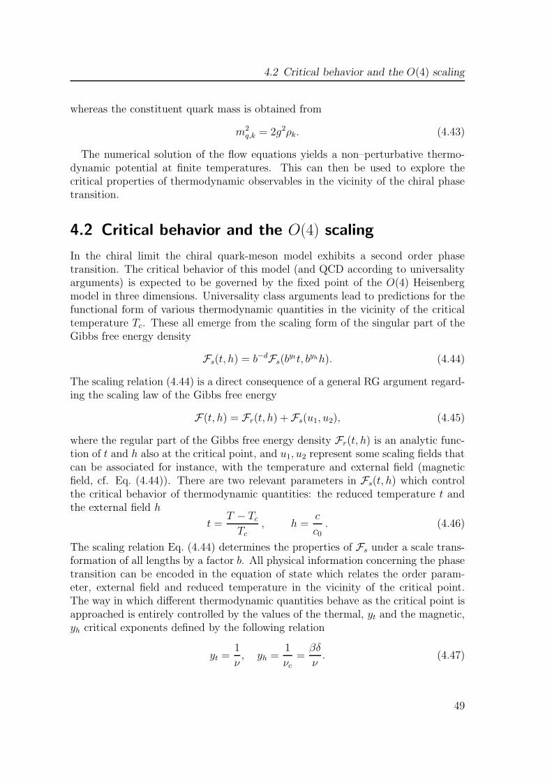
4.2 Critical behavior and the O(4) scaling
whereas the constituent quark mass is obtained from
m2q,k = 2g2ρk. (4.43)
The numerical solution of the flow equations yields a non–perturbative thermo-dynamic potential at finite temperatures. This can then be used to explore thecritical properties of thermodynamic observables in the vicinity of the chiral phasetransition.
4.2 Critical behavior and the O(4) scaling
In the chiral limit the chiral quark-meson model exhibits a second order phasetransition. The critical behavior of this model (and QCD according to universalityarguments) is expected to be governed by the fixed point of the O(4) Heisenbergmodel in three dimensions. Universality class arguments lead to predictions for thefunctional form of various thermodynamic quantities in the vicinity of the criticaltemperature Tc. These all emerge from the scaling form of the singular part of theGibbs free energy density
Fs(t, h) = b−dFs(bytt, byhh). (4.44)
The scaling relation (4.44) is a direct consequence of a general RG argument regard-ing the scaling law of the Gibbs free energy
F(t, h) = Fr(t, h) + Fs(u1, u2), (4.45)
where the regular part of the Gibbs free energy density Fr(t, h) is an analytic func-tion of t and h also at the critical point, and u1, u2 represent some scaling fields thatcan be associated for instance, with the temperature and external field (magneticfield, cf. Eq. (4.44)). There are two relevant parameters in Fs(t, h) which controlthe critical behavior of thermodynamic quantities: the reduced temperature t andthe external field h
t =T − TcTc
, h =c
c0. (4.46)
The scaling relation Eq. (4.44) determines the properties of Fs under a scale trans-formation of all lengths by a factor b. All physical information concerning the phasetransition can be encoded in the equation of state which relates the order param-eter, external field and reduced temperature in the vicinity of the critical point.The way in which different thermodynamic quantities behave as the critical point isapproached is entirely controlled by the values of the thermal, yt and the magnetic,yh critical exponents defined by the following relation
yt =1
ν, yh =
1
νc=βδ
ν. (4.47)
49

4 Critical phenomena and O(4) scaling
The critical exponents are used to describe the behavior of various physical observ-ables in the vicinity of a critical temperature Tc. In this region physical observablesshow a power law behavior characterized by the corresponding critical exponent.There are many critical exponents (α, β, δ, γ, ν, η) and some of them we calculatelater in the following subsections. Here we mention also the so called hyperscalingrelations that the critical exponents satisfy
δ − 1 =γ
β, (4.48a)
γ = ν(2 − η), (4.48b)
dν = β(1 + δ), (4.48c)
α = 2 − dν. (4.48d)
The scaling relations Eqs.(4.48b) and (4.48d) are known as Fisher’s and Josephson’slaw respectively. We should note here the fact that Eq. (4.48d) is not valid for d > 4.
4.2.1 Order parameter
A phase transition involving spontaneous symmetry breaking, is signaled by thevanishing of an order parameter, when approached from the broken symmetry phase.In the quark meson model, a possible order parameter related with chiral symmetrybreaking is obtained by differentiating the free energy with respect to the externalfield h. Thus, it follows from Eqs. (2.22) and (4.3) that the order parameter can beidentified with the thermodynamic average of the sigma field
〈σ〉 =√
2ρ0. (4.49)
In the FRG approach, the 〈σ〉 is directly obtained from the flow equation (4.41b).Indeed, for a given temperature T by solving the set of coupled flow equations we get〈σ〉 by substituting for ρ0 the value of ρk obtained at the end of the flow (k → 0). Inthis way the order parameter contains the relevant contributions from fluctuations.
In Fig. 4.1 we show the resulting order parameter dependence on the reducedtemperature t and for different values of the external field h. In the chiral limit i.e.for h = 0, the order parameter 〈σ〉 smoothly decreases with increasing T and finallyvanishes exactly at the critical temperature where t = 0. This is a typical behaviorthat is expected in a system with the second order phase transition. For the finiteh, the chiral symmetry of the Lagrangian is explicitly broken. The external field de-stroys the second order phase transition which turns into a crossover. Consequently,for small h, 〈σ〉 still shows a very abrupt change in a narrow temperature interval, atthe so called pseudo-critical temperature. However, in this case the order parameterremains non-zero, even at very high temperatures, as seen in Fig. 4.1. Consequently,for h 6= 0 there is no true phase transition.
50
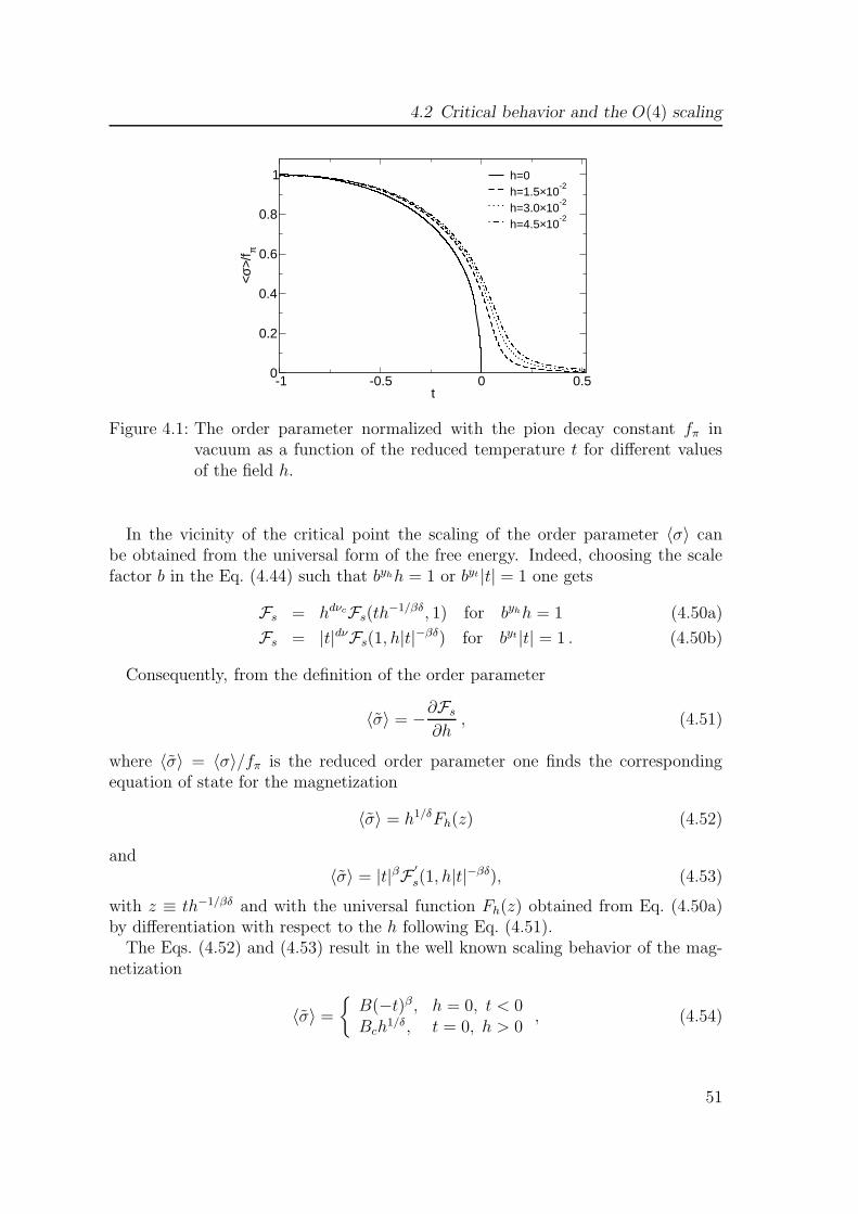
4.2 Critical behavior and the O(4) scaling
-1 -0.5 0 0.5t
0
0.2
0.4
0.6
0.8
1
<σ>/
f π
h=0h=1.5×10
-2
h=3.0×10⁻²
h=4.5×10⁻²
Figure 4.1: The order parameter normalized with the pion decay constant fπ invacuum as a function of the reduced temperature t for different valuesof the field h.
In the vicinity of the critical point the scaling of the order parameter 〈σ〉 canbe obtained from the universal form of the free energy. Indeed, choosing the scalefactor b in the Eq. (4.44) such that byhh = 1 or byt |t| = 1 one gets
Fs = hdνcFs(th−1/βδ, 1) for byhh = 1 (4.50a)
Fs = |t|dνFs(1, h|t|−βδ) for byt|t| = 1 . (4.50b)
Consequently, from the definition of the order parameter
〈σ〉 = −∂Fs
∂h, (4.51)
where 〈σ〉 = 〈σ〉/fπ is the reduced order parameter one finds the correspondingequation of state for the magnetization
〈σ〉 = h1/δFh(z) (4.52)
and〈σ〉 = |t|βF ′
s(1, h|t|−βδ), (4.53)
with z ≡ th−1/βδ and with the universal function Fh(z) obtained from Eq. (4.50a)by differentiation with respect to the h following Eq. (4.51).
The Eqs. (4.52) and (4.53) result in the well known scaling behavior of the mag-netization
〈σ〉 =
B(−t)β , h = 0, t < 0Bch
1/δ, t = 0, h > 0, (4.54)
51

4 Critical phenomena and O(4) scaling
-14 -12 -10log(t)
-5
-4
-3
log(
<σ>/
f π)
-36 -34 -32 -30log(h)
-7.5
-7
-6.5
-6
log(
<σ>/
f π)
Figure 4.2: The critical exponent β (left panel) and δ (right panel). See text fordetails.
where B and Bc are the amplitudes of the magnetization at the critical point (t = 0)and at the so called coexistence line (t < 0, h = 0) [78]. The scaling behavior of theorder parameter in the chiral limit, when approaching the critical temperature t = 0from below, is controlled by the critical exponent β. Thus, β can be obtained as theslope of the logarithm of 〈σ〉 if plotted as a function of log(t). On the other hand,the critical exponent δ controls the scaling behavior of 〈σ〉 at the critical point t = 0as h→ 0.
Fig. 4.2 shows the scaling properties of 〈σ〉 close to the critical point (t → 0) forvanishing external field as well as the scaling with h at the (pseudo)critical point(t = 0).
In both cases the order parameter calculated in the quark-meson model withinthe FRG method shows a scaling behavior that is expected from the Eq. (4.44).This demonstrates that, in the parameter range considered, the free energy of thequark-meson model is dominated by the singular part (cf. Eq. (4.44)). Applyinga linear logarithmic fit to the results from Fig. 4.2 we have obtained the followingvalues for the critical exponents
β ≃ 0.402 and δ ≃ 4.818. (4.55)
In the mean field approximation one also finds scaling of the order parameter〈σ〉 close to the critical point, but with different critical exponents, β = 0.5 andδ = 3. Thus, the singularity at the chiral phase transition is modified substantiallyby fluctuations.
The values (4.55) of β and δ obtained from the fit to the functional dependencies of〈σ〉 shown in the Fig. 4.2 are consistent with that expected in the O(4) universalityclass. Indeed, in a Monte Carlo simulation of the three-dimensional O(4) spin model,Kanaya and Kaya [76] find β = 0.3836(46) and δ = 4.851(22). The agreement with
52

4.2 Critical behavior and the O(4) scaling
-1e-05 0 1e-05t
-2
-1
0
1
Rh
<σ>
1e-18 1e-15 1e-12 1e-09 1e-06h
0
0.1
0.2
0.3
0.4
0.5
t=-3.2×10⁻⁶
t=-2.6×10⁻⁶
t=-1.9×10⁻⁶
Rh
<σ>
Figure 4.3: The left-hand figure: the ratio Rh〈σ〉 as a function of t calculated at fixed
h = 5.65× 10⁻¹³. The right-hand figure: the ratio as a function of h forthree different values of the reduced temperature t.
this precision calculation is satisfactory, given our simple Ansatz. Consequently, weconclude that the critical properties of the chiral order parameter in the quark-mesonmodel are indeed governed by the O(4) universality class. Our results, obtained inthe relatively simple LPA, illustrate the efficiency of the FRG approach to correctlyaccount for a non-perturbative, long distance physics near a phase transition.
In the formulation of the flow equation for the quark-meson model we have ne-glected the wavefunction renormalization for both bosonic and fermionic fields. Thecoincidence of our critical exponents for chiral order parameter with O(4) latticeresults as well as with the previous studies [61] which account for anomalous di-mension in the FRG flow, indicates that this effect is not of particular relevancewhen quantifying the singular properties of the order parameter at the chiral phasetransition.
So far we have discussed the scaling of the order parameter 〈σ〉 with t for h = 0in the chirally broken phase and with h at t = 0. In the chiral limit, the orderparameter vanishes identically in the symmetric phase, i.e. for t > 0. Thus, theorder parameter does not exhibit a singularity when the critical point is approachedfrom above. However, since for h 6= 0 the order parameter is always non-zero, it isinteresting to explore its behavior for small but finite values of h, when the criticalpoint is approached from the broken (t < 0) as well as from the symmetric (t > 0)phase. The scaling behavior is in this case characterized by a so-called effectivecritical exponent [69, 70].
For a given h, this exponent is defined by
Rh〈σ〉 ≡
d log 〈σ〉d log t
=t
〈σ〉∂〈σ〉∂t
. (4.56)
53
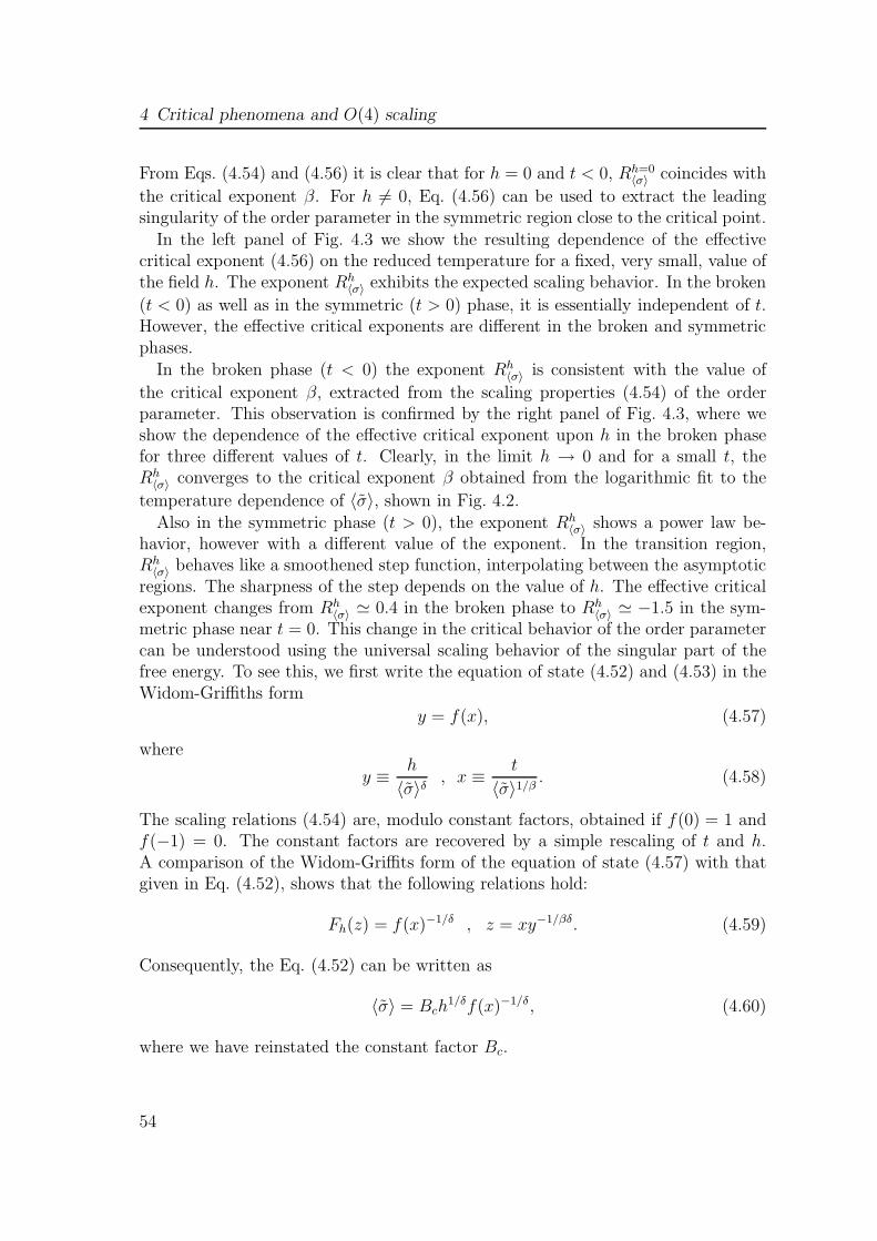
4 Critical phenomena and O(4) scaling
From Eqs. (4.54) and (4.56) it is clear that for h = 0 and t < 0, Rh=0〈σ〉 coincides with
the critical exponent β. For h 6= 0, Eq. (4.56) can be used to extract the leadingsingularity of the order parameter in the symmetric region close to the critical point.
In the left panel of Fig. 4.3 we show the resulting dependence of the effectivecritical exponent (4.56) on the reduced temperature for a fixed, very small, value ofthe field h. The exponent Rh
〈σ〉 exhibits the expected scaling behavior. In the broken
(t < 0) as well as in the symmetric (t > 0) phase, it is essentially independent of t.However, the effective critical exponents are different in the broken and symmetricphases.
In the broken phase (t < 0) the exponent Rh〈σ〉 is consistent with the value of
the critical exponent β, extracted from the scaling properties (4.54) of the orderparameter. This observation is confirmed by the right panel of Fig. 4.3, where weshow the dependence of the effective critical exponent upon h in the broken phasefor three different values of t. Clearly, in the limit h → 0 and for a small t, theRh
〈σ〉 converges to the critical exponent β obtained from the logarithmic fit to the
temperature dependence of 〈σ〉, shown in Fig. 4.2.Also in the symmetric phase (t > 0), the exponent Rh
〈σ〉 shows a power law be-havior, however with a different value of the exponent. In the transition region,Rh
〈σ〉 behaves like a smoothened step function, interpolating between the asymptoticregions. The sharpness of the step depends on the value of h. The effective criticalexponent changes from Rh
〈σ〉 ≃ 0.4 in the broken phase to Rh〈σ〉 ≃ −1.5 in the sym-
metric phase near t = 0. This change in the critical behavior of the order parametercan be understood using the universal scaling behavior of the singular part of thefree energy. To see this, we first write the equation of state (4.52) and (4.53) in theWidom-Griffiths form
y = f(x), (4.57)
where
y ≡ h
〈σ〉δ , x ≡ t
〈σ〉1/β . (4.58)
The scaling relations (4.54) are, modulo constant factors, obtained if f(0) = 1 andf(−1) = 0. The constant factors are recovered by a simple rescaling of t and h.A comparison of the Widom-Griffits form of the equation of state (4.57) with thatgiven in Eq. (4.52), shows that the following relations hold:
Fh(z) = f(x)−1/δ , z = xy−1/βδ. (4.59)
Consequently, the Eq. (4.52) can be written as
〈σ〉 = Bch1/δf(x)−1/δ, (4.60)
where we have reinstated the constant factor Bc.
54

4.2 Critical behavior and the O(4) scaling
This equation of state can be used to explore the scaling properties of 〈σ〉 whenapproaching the critical point from the symmetric phase. For t > 0 and for h →0, the chiral order parameter (normalized to its value in vacuum) is very small.Consequently, the argument x of the function f(x) in equation (4.60) is very largeand the scaling behavior of 〈σ〉 for t > 0 and for small but finite h is determined bythe asymptotic form of the scaling function f(x) for x → ∞. In this limit, f(x) isgiven by Griffiths’ analyticity condition [79],
f(x) =∞∑
n=1
fnxγ−2(n−1)β . (4.61)
Approximating the scaling function f(x) by the leading term, f(x) ≃ xγ and follow-ing the Eq. (4.60), one finds that for t > 0 and h → 0 the equation of state scalesas
〈σ〉 = Bch1/δf(x)−1/δ ∼ h1/δx−γ/δ
= h1/δ(t〈σ〉−1/β
)−γ/δ
= h1/δt−γ/δ〈σ〉γ/βδ. (4.62)
From the last line in (4.62) one has
〈σ〉1−γ/βδ = h1/δt−γ/δ −→ 〈σ〉 = t−γh, (4.63)
where we have used the hyperscaling relation Eq. (4.48a). Thus, for t > 0 andh 6= 0, the order parameter diverges for t→ 0, while for h = 0 it vanishes identically,indicating that this equation remains correct also in the chiral limit.
From the scaling behavior of 〈σ〉 shown in the left panel of Fig. 4.3, we findγ ≃ 1.6. This is consistent with the lattice result for the O(4) spin system obtained inRef. [76], γ ≃ 1.5. Thus, the FRG method applied to the quark meson model yieldsa scaling behavior of the order parameter, which is consistent with that found forthe O(4) universality class. This is the case at the critical point, on the coexistenceline and when approaching the critical point from the high temperature phase for afinite value of the external magnetic field.
4.2.2 Chiral susceptibility
The critical properties of a thermodynamic system can be explored by studying thefluctuations of various observables. In particular, the fluctuations of the order pa-rameter are a sensitive probe of the order of the phase transition and the positionof a possible critical end point. In statistical physics, fluctuations are reflected inthe corresponding susceptibilities χ. In the case of the chiral order parameter, thecorresponding susceptibility is defined as the response to a change of the external
55

4 Critical phenomena and O(4) scaling
-0.0005 0 0.0005t
0
5
10
15
20
25
χ σ/106
h=6.0×10⁻⁹
h=9.0×10⁻⁹
h=1.2×10⁻⁸
h=1.5×10⁻⁸
Figure 4.4: Normalized susceptibility χσ as a function of the reduced temperature tfor different values of the field h.
field h; the susceptibility χ is obtained by taking the second derivative of the effec-tive potential with respect to h. The susceptibility in other channels is computedanalogously. It follows that the susceptibilities are inversely proportional to the cor-responding mass squared. Consequently, the divergence of a susceptibility, e.g. atthe critical end point, signals a zero-mass mode of some effective field.
In the chiral quark-meson model, we are not only dealing with a massless sigmafield but also with a pseudo-Goldstone mode, controlled by the pion mass. Thesigma and the pion represent the longitudinal and transverse modes of the O(4)field φ, respectively. Consequently, one distinguishes between the longitudinal andtransverse order parameter susceptibilities.
The longitudinal susceptibility is introduced as the usual derivative of the mag-netization with respect to the external field
χl = χσ =∂〈σ〉∂h
, (4.64)
whereas the transverse susceptibility, which is directly related to the fluctuation ofthe Goldstone modes, is obtained from
χt = χπ =〈σ〉h. (4.65)
The latter expression is a direct consequence of the O(4) invariance of the free energyfor h = 0 and follows from the corresponding Ward identity [74].
The critical behavior of the longitudinal and transverse chiral susceptibility canbe obtained from the scaling form of the singular part of the free energy or directly
56

4.2 Critical behavior and the O(4) scaling
-26 -24 -22 -20log(h)
-13
-12
-11
-10
-9
log(
t max
)
-13 -12 -11 -10log(tmax)
18
20
22
log(
χ σmax
)
Figure 4.5: Scaling of the pseudo-critical temperature corresponding to the maxi-mum of the χσ (left panel) and the scaling of the maxima of χσ (rightpanel).
from the magnetic equation of state (4.60). In Fig. 4.4 we show the longitudinalsusceptibility normalized to its value in vacuum (χσ/χ0) as a function of the re-duced temperature for several values of the symmetry breaking field h. At finite h,this susceptibility shows a peak structure with a maximum at the pseudo-criticaltemperature tmax(h). With decreasing h, there is a shift of tmax and an increase ofthe fluctuations at the pseudo-critical point. In the chiral limit χσ diverges at thetransition temperature, because the mass of the sigma field vanishes.
Using the results shown in the Fig. 4.4, one can define a pseudo-critical line in the(t, h)-plane that characterizes the dependence of the transition temperature tmax
on the symmetry breaking field h. Renormalization group arguments imply thatthe pseudo-critical temperature and the maximum of the longitudinal susceptibilityshould exhibit universal scaling according to [75]:
tmax(h) ≃ Tph1/(γ+β), χσ(tmax, h) ≃ Cpt
−γmax, (4.66)
with O(4) critical exponents.In Fig. 4.5 we confront the scaling behavior of the susceptibility with Eq. (4.66).
The critical exponents are extracted by performing a linear logarithmic fit to thepseudo-critical temperature and the maximum value of the susceptibility. We find,
1/(γ + β) = 0.494 and γ = 1.618 ,
which implies β = 0.406, in good agreement with the results obtained above usingEqs. (4.54) and (4.63). Thus, the scaling of χσ with the symmetry breaking field his also consistent with O(4) universality.
In the symmetric phase the longitudinal and the transversal susceptibility shouldcoincide (χσ = χπ). In addition, the strength of the singularities of both these
57

4 Critical phenomena and O(4) scaling
-12 -11 -10 -9log(t)
18
20
22
log(
χ σ)
Figure 4.6: The logarithm of the susceptibility for h→ 0 for different values of log(t)in the symmetric phase. The solid line is a linear fit.
susceptibilities at the critical point t = 0 should be controlled by the same criticalexponents. To find the right scaling behavior of susceptibilities when approachingthe critical point from the symmetric phase we use the Widom-Griffits form of theequation of state (4.60) together with the large-x expansion of the scaling functionf(x). From Eqs. (4.63), (4.64) and (4.65) it is clear that in the symmetric phase(t > 0) and h→ 0
χσ = χπ ≃ t−γ . (4.67)
Thus, when approaching the critical point from the symmetric phase the scalingbehavior of the longitudinal and transverse susceptibility should be controlled bythe critical exponent γ. Fig. 4.6 shows the scaling behavior of the susceptibility fort > 0 and in the limit of h→ 0. From the slope of the line we obtain
γ = 1.575.
This value of the critical exponent γ differs only slightly from that obtained whenanalyzing the scaling of the maxima of the χσ following the Eq. (4.66). One of thereasons for this small difference can be traced back to the problem with an exactdetermination of the critical temperature.
In the broken phase, along the coexistence line, the longitudinal and transversesusceptibilities show different critical behavior. In the chiral limit, the order param-eter is finite in the broken phase as long as t < 0. Thus, knowing that the transversesusceptibility χπ is directly related to the order parameter through Eq. (4.65), oneexpects that it diverges as
χπ ∼ h−1 for T < Tc (4.68)
58

4.2 Critical behavior and the O(4) scaling
due to the appearance of the Goldstone bosons. A less obvious result is the expecteddivergence of the longitudinal susceptibility on the coexistence line where the leadingorder term has a divergence of the form [57]
χσ ∼ h−1/2 for T < Tc. (4.69)
The scaling properties of the longitudinal and the transverse susceptibilities canbe directly obtained from the Widom-Griffiths form of the equation of state. Let usstart with the longitudinal susceptibility χσ that has the following scaling
χσ = Bch1/δ−1 βf(x)1−1/δ
βδf(x) − xf ′(x). (4.70)
Starting from Eqs. (4.60) and (4.64) we have
χσ =∂〈σ〉∂h
=∂
∂h
(Bch
1/δf(x)−1/δ)
=1
δBch
1/δ−1f(x)−1/δ − 1
δBch
1/δf(x)−1/δ−1f ′(x)∂x
∂h. (4.71)
In order to proceed, we have to find the derivative ∂x/∂h. Indeed, using Eq (4.58)one gets
∂x
∂h=
∂
∂h
(t
〈σ〉1/β)
= − t
β
1
〈σ〉1/β+1
∂〈σ〉∂h
= −xβ
1
〈σ〉χσ. (4.72)
Now, plugging this result back into Eq. (4.71) yields the following expression
χσ =1
δBch
1/δ−1f(x)−1/δ +Bch1/δ x
βδ
1
〈σ〉f(x)−1/δ−1f ′(x)χσ
=1
δBch
1/δ−1f(x)−1/δ +x
βδf(x)−1f ′(x)χσ (4.73)
where we have used Eq. (4.60) in the last step. By solving the above equation forχσ, we finally obtain Eq. (4.70). For the scaling of the transverse susceptibility χπone gets
χπ = Bch1/δ−1f(x)−1/δ, (4.74)
which is trivial to obtain using Eqs. (4.60) and (4.65).Now, we will scrutinize the behavior of susceptibilities in the broken phase. It has
been already mentioned that both, χσ and χπ diverge as h−1/2 and h−1 respectivelyfor all T < Tc. Indeed, from the scaling behavior of 〈σ〉 in the broken phase i.e. atthe coexistence line (4.54) and using Eq. (4.65) follows
χπ ∼ h−1(−t)β . (4.75)
This scaling behavior could also be obtained from Eq. (4.74). The scaling of χσ isless trivial to obtain, but still feasible and fortunately, not tedious. However, some
59

4 Critical phenomena and O(4) scaling
approximation of the scaling function f(x) has to be used. In the vicinity to thecoexistence line where x → −1 the scaling function was shown to behave as [78]
f(x) ≈ (1 + x)2, (4.76)
with1 + x = a1y
1/2 + a2y + . . . (4.77)
for the system in three dimensions. Having these results at hand, Eq. (4.70) can berewritten as
χσ ≃ h1/δ−1 (1 + x)2−2/δ
βδ(1 + x)2 − 2x(1 + x)= h1/δ−1 (1 + x)1−2/δ
βδ(1 + x) − 2x≃ h1/δ−1(1 + x)1−2/δ.
(4.78)In the last step we have used the fact that the denominator is approximately constantfor x = −1. Now, the next approximation we use is Eq. (4.77) that together withEq. (4.58) yields
χσ ≃ h1/δ−1y1/2−1/δ = h1/δ−1(h〈σ〉−δ
)1/2−1/δ= h−1/2〈σ〉−δ/2+1. (4.79)
Again, we make use of our knowledge of how 〈σ〉 scales for T < Tc given by Eq. (4.54)and finally obtain
χσ ∼ h−1/2(−t)β−(βδ)/2. (4.80)
Consequently, Eqs. (4.80) and (4.75) clearly show, how the longitudinal and trans-verse susceptibilities diverge in the broken phase and near the coexistence line.Fig. 4.7 shows the behavior of the longitudinal and transverse susceptibilities as afunction of t and h near the coexistence line as obtained in the quark meson modelwithin the FRG method. Both susceptibilities show the scaling behavior as expectedfrom the Eqs. (4.80) and (4.75). From the linear fit to the results in the Fig. 4.7–leftwe get the values 0.499 and 1.000 for the critical exponents of the χσ and χπ suscep-tibilities respectively. These results are in excellent agreement with that expectedfrom the Eqs. (4.80) and (4.75). The corresponding fit to χσ and χπ in Fig. 4.7-rightgives,
(β − βδ/2) = −0.617 and β = 0.395,
the values that are also consistent with our previous findings for the critical expo-nents β and δ calculated from the scaling of the order parameter.
In order to show the scaling behavior of the longitudinal and transverse suscepti-bility in a broad parameter range which covers the broken and symmetric phase weintroduce the ratio
Rhχπ,σ
=t
χπ,σ
∂χπ,σ∂t
(4.81)
for the transverse χπ and the longitudinal χσ susceptibilities. The quantity Rhχπ,σ
,similarly to (4.56) defines an effective critical exponent. In the Fig. 4.8 we summa-rized the t and h dependence of the Rh
χπand Rh
χσin the vicinity of the critical point.
60

4.2 Critical behavior and the O(4) scaling
-32 -30 -28log(h)
10
20
30
40
log(
χ)
σπ
-12 -10 -8log(t)
20
22
24
log(
χ)
σπ
Figure 4.7: Critical exponents for the χσ and χπ in the broken phase (t < 0) closeto the critical point. See text for details.
In the left-hand figure we illustrate how the critical exponents of the susceptibilitiesare changing from the broken to symmetric phase for a fixed h. In the right-handfigure we show the h–dependence of Rh
χπ,σin the symmetric phase for a few values
of t.In the symmetric phase χπ and χσ coincide, thus their critical behavior is deter-
mined by the same exponent (γ ∼ 1.58) as obtained from the Fig. 4.8-left. Thisscaling of Rh
χπ,σis also shown in the Fig. 4.8-right for fixed t > 0 as a function of h.
In the broken phase (see Fig. 4.8–left) there is a clear splitting in the numericalvalues of the critical exponents,
Rhχπ
∼ β
andRhχσ
∼ β(1 − δ/2)
indicating a different sensitivity of the longitudinal and the transverse susceptibilitiesto the chiral symmetry breaking.
The coincidence of the transverse and longitudinal susceptibilities and their similarscaling properties at the transition point, can be used to directly obtain the criticalexponent δ [71, 72, 73]. Indeed, considering the ratio of χπ and χσ such that
∆(t, h) =χ−1π
χ−1σ
=hχσ〈σ〉 (4.82)
and applying the scaling behavior of the chiral susceptibilities one finds that
limh→0
∆(t, h) =
1, t > 01/δ, t = 00, t < 0
(4.83)
61
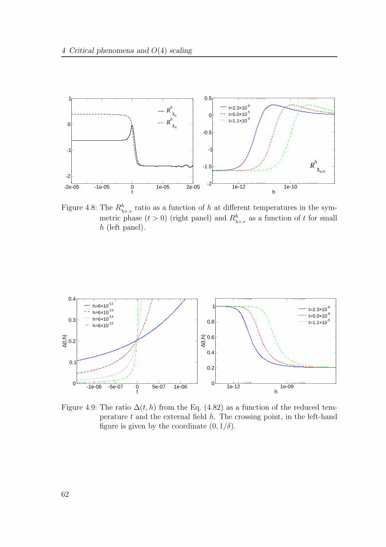
4 Critical phenomena and O(4) scaling
-2e-05 -1e-05 0 1e-05 2e-05t
-2
-1
0
1
Rh
χσ
Rh
χπ
1e-12 1e-10h
-2
-1.5
-1
-0.5
0
0.5
t=2.3×10⁻⁶
t=5.0×10⁻⁵
t=1.1×10⁻⁵
Rh
χσ,π
Figure 4.8: The Rhχσ,π
ratio as a function of h at different temperatures in the sym-
metric phase (t > 0) (right panel) and Rhχσ,π
as a function of t for smallh (left panel).
-1e-06 -5e-07 0 5e-07 1e-06t
0
0.1
0.2
0.3
0.4
∆(t,h
)
h=6×10-12
h=6×10-13
h=6×10-14
h=6×10-15
1e-12 1e-09h
0
0.2
0.4
0.6
0.8
1
∆(t,h
)
t=2.3×10⁻⁶
t=5.0×10⁻⁶
t=1.1×10⁻⁵
Figure 4.9: The ratio ∆(t, h) from the Eq. (4.82) as a function of the reduced tem-perature t and the external field h. The crossing point, in the left-handfigure is given by the coordinate (0, 1/δ).
62

4.2 Critical behavior and the O(4) scaling
Consequently, ∆(t, h) can be used to directly extract the value of the criticalexponent δ without any logarithmic fits. In addition, this ratio can also be used tofind a position of the critical point where all ∆(t, h) are plotted as a function of tfor different values of h crosses.
In the Fig. 4.9-left we show the resulting behavior of ∆(t, h) as a function of t fordifferent values of h. As expected all lines for different h cross at t = 0 giving
δ ≈ 4.91.
This value slightly deviates from that obtained previously using a logarithmic fitbut agrees better with the LGT expectations [71].
Fig. 4.9-right shows the scaling of ∆(t, h) as a function of h for fixed t > 0. In thechiral limit, that is for h = 0 the longitudinal and transverse susceptibility coincide,thus ∆(t, h) = 1 as seen in this figure. On the other hand for h→ ∞, ∆(t, h) → 1/δ.The last behavior is a direct consequence of the equation of state (4.53) and thedefinition (4.82). Indeed, from these equations one finds that
∆(t, h) =hχσ
tβF ′
s(1, ht−βδ)
≃ F (h/tβδ) ,
with F (x) being some scaling function. Consequently, the limits t → 0 at finite hor h→ ∞ at finite t should result in the same value of ∆(t, h).
4.2.3 Correlation length
The phase transition can be identified not only by considering the critical behaviorof the order parameter or its susceptibilities, but also the correlation length ξ whichgoverns the exponential decay of the correlation function. The correlation length isquantified by the relevant mass scale in a system. In the chiral model consideredhere, there are two relevant mass scales, the transverse mass connected to the pionand the longitudinal mass related to the sigma field. Consequently, one introducesthe transverse ξπ and the longitudinal ξσ correlation lengths. In the critical regionthe ξt and ξl can also be connected with the corresponding susceptibilities [77]
χl ∼ ξ2l , χt ∼ ξ2
t . (4.84)
Consequently, in the chiral quark-meson model, the correlation lengths are connectedwith the pion and the sigma masses
ξσ ∼ 1
mσ, ξπ ∼ 1
mπ. (4.85)
Fig. 4.10 shows the correlation lengths, ξσ and ξπ calculated at the critical pointt = 0 as a function of the external field h. Both, ξσ and ξπ diverge as h → 0. This
63
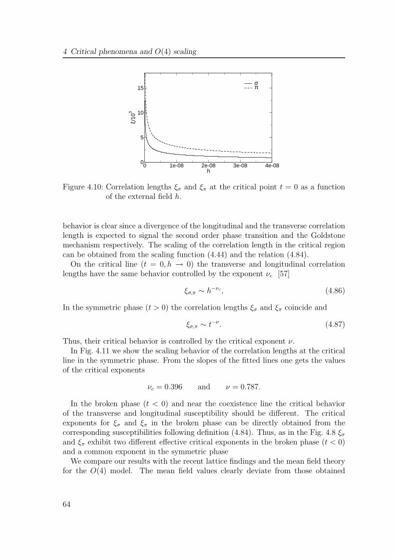
4 Critical phenomena and O(4) scaling
0 1e-08 2e-08 3e-08 4e-08h
0
5
10
15
ξ/10
3
σπ
Figure 4.10: Correlation lengths ξσ and ξπ at the critical point t = 0 as a functionof the external field h.
behavior is clear since a divergence of the longitudinal and the transverse correlationlength is expected to signal the second order phase transition and the Goldstonemechanism respectively. The scaling of the correlation length in the critical regioncan be obtained from the scaling function (4.44) and the relation (4.84).
On the critical line (t = 0, h → 0) the transverse and longitudinal correlationlengths have the same behavior controlled by the exponent νc [57]
ξσ,π ∼ h−νc , (4.86)
In the symmetric phase (t > 0) the correlation lengths ξσ and ξπ coincide and
ξσ,π ∼ t−ν . (4.87)
Thus, their critical behavior is controlled by the critical exponent ν.In Fig. 4.11 we show the scaling behavior of the correlation lengths at the critical
line in the symmetric phase. From the slopes of the fitted lines one gets the valuesof the critical exponents
νc = 0.396 and ν = 0.787.
In the broken phase (t < 0) and near the coexistence line the critical behaviorof the transverse and longitudinal susceptibility should be different. The criticalexponents for ξσ and ξπ in the broken phase can be directly obtained from thecorresponding susceptibilities following definition (4.84). Thus, as in the Fig. 4.8 ξσand ξπ exhibit two different effective critical exponents in the broken phase (t < 0)and a common exponent in the symmetric phase
We compare our results with the recent lattice findings and the mean field theoryfor the O(4) model. The mean field values clearly deviate from those obtained
64

4.3 Conclusions
-32 -30 -28 -26log(h)
10
12
14
log(
ξ)
σπ
-12 -11 -10 -9log(t)
8
9
10
11
log(
ξ)Figure 4.11: The critical exponent νc for correlation lengths ξσ and ξπ on the critical
line t = 0 (left panel) and the critical exponent ν in the symmetricphase t > 0 (right panel). The solid lines represent linear fits.
within the FRG approach, showing the importance of quantum fluctuations nearthe critical point. Our results for different critical exponents are found to be in aquite good agreement with the Monte Carlo lattice results [76] in spite of the fact,that we have neglected the anomalous dimension terms in the flow equation. Thescale η, of the anomalous dimension defined as
η ≡ − ∂
∂tlogZ, (4.88)
where Z is the wavefunction renormalization can be extracted through the hyper-scaling relation
δ =d+ 2 − η
d− 2 + η, (4.89)
which together with our value for δ results in
η ≈ 0.031.
This result appears in the range obtained within LGT calculations where (η =0.0254 [76]). The small value of η explains why the anomalous dimension leads toa rather small corrections for different exponents and the scaling properties of thephysical observables within the FRG approach. We have summarized our results fordifferent critical exponents in Table 4.1.
4.3 Conclusions
In this chapter we have discussed the critical properties of the quark-meson effectivemodel related with the chiral phase transition at finite temperature. We have focused
65

4 Critical phenomena and O(4) scaling
β δ γ ν νc αO(4) latticea 0.3836 4.851 1.477 0.7479 0.4019b -0.244Mean Field 0.5 3 1 0.5 1/3 0
FRG (our work) 0.397(2) 4.818 1.603(9) 0.801(47) 0.396 -0.361b
Table 4.1: The critical exponents for the O(4) model from the FRG studies, theLGT and the mean-field calculations. The quoted errors in our resultsare due to different methods that were used to find the critical exponents(see text); adata taken from [76]; bfrom the hyperscaling relations.
on the universal scaling behavior of different physical quantities. In order to correctlyaccount for the quantum fluctuations and non-perturbative effects we have appliedthe functional renormalization group method. Deriving the flow equation for thescale dependent thermodynamic potential at finite temperature and density in thepresence of an external field we have used the polynomial truncation method tosolve this equation numerically. We have shown, that with our particular choice ofthe optimized regulator functions this method provides numerically stable results.We have neglected the bosonic and fermionic wave function renormalization and therunning of the Yukawa coupling. However, we have argued, that such effects leadonly to the sub-leading corrections to a scaling near the phase transition.
Within the scope of our investigations, we have calculated different thermody-namical quantities that are sensitive to the chiral phase transition. In particular, wehave analyzed the scaling behavior of the chiral order parameter, its longitudinal andtransverse susceptibilities as well as the correlation lengths in the chiral limit and inthe presence of an external field. The results show that the chiral order parameterand its susceptibilities scale near the chiral phase transition following the universalscaling behavior of the singular part of the free energy. Here we have extracted thecorresponding critical exponents at the critical point and at the coexistence line andhave also analyzed the scaling of the pseudocritical temperature and the maxima ofthe longitudinal susceptibility at the finite external field.
As the most interesting case we have analyzed the leading scaling behavior of thelongitudinal and transverse susceptibilities and their different ratios when approach-ing the critical point from the symmetric and the broken phase with finite externalfield. Our results show that this scaling is consistent with the Widom-Griffiths mag-netic equation of state in the systematic ǫ-expansion of the scaling function. Thecritical exponents obtained in this work are in a very good agreement with the re-cent LGT results obtained for the O(4) spin system. This confirms the expectationsthat the chiral phase transition of the 2-flavor effective chiral Lagrangian belongsto the O(4) universality class. This also supports the validity of the FRG approachand the truncation methods of the flow equation used in our calculations to cor-
66
4.3 Conclusions
rectly account for the quantum fluctuations and the non-perturbative long distancedynamics near the chiral phase transition.
67

68

Chapter 5
Thermodynamics of hot and dense
matter
During recent years the importance of studying the phase structure of strongly inter-acting matter has been widely recognized. The phase diagram of a thermodynamicsystem may be mapped out by studying fluctuations and their response to changes ofthe thermodynamic parameters. Understanding the critical properties of the QCDmedium and its phase diagram is a central problem in strong interaction physics,which is being addressed in both theoretical and experimental studies. The phasediagram of QCD, a theory that is considered to govern the strong interaction, can beaccessed experimentally in heavy-ion collision experiments at the BNL RelativisticHeavy-Ion Collider (RHIC), the CERN Super Proton Synchrotron (SPS) and theLarge Hadron Collider (LHC). It is expected that under extreme conditions such ashigh temperature and/or density the vacuum of strongly interacting matter changes,rendering novel phases. One usually speaks of a chirally symmetric or deconfinedphase or a color superconducting phase. These phase transitions are also very im-portant in the physics of the early universe and for understanding the compositionand properties of compact stars. A proper understanding of the phase diagram ofstrongly interacting matter will be an important step towards the clarification ofthe dynamics of QCD. The most important and at the same time highly intriguingphenomena of QCD in the nonperturbative regime are chiral symmetry breakingand confinement. The interplay of the two is still an open issue and the subject ofimmense interest. Usually one speaks of two different QCD phase transitions thattake place if either the temperature or the density crosses some critical point. Eachtransition is well defined in some limit of QCD. In the limit of infinite quark massesthe deconfinement phase transition occurs. On the other hand, for vanishing quarkmasses, the chiral (symmetry-restoring) phase transition takes place instead. For
69
5 Thermodynamics of hot and dense matter
physical quark masses, neither of the two transitions is, due to the explicit symme-try breaking, strictly speaking a phase transition. Nevertheless, the correspondingcrossover transition can be identified by studying the relevant susceptibilities. Theunderlying reason for the coincidence of the two transitions, observed in lattice QCDcalculations, is presently subject of intense investigations.
In order to give satisfying answers to a variety of questions regarding the originand nature of QCD phase transitions quite a few theoretical and phenomenologicalmodels and approaches have been developed and during the years further extendedand improved. Lattice Gauge Theory (LGT), in particular, has provided substantialinsight into the physics of the transition between the low temperature hadronicand high temperature quark-gluon plasma phase [80, 83, 84, 85, 86, 87, 88, 89,90, 91, 45, 81, 82]. Effective models also provide a useful qualitative descriptionof the chiral phase transition [43, 24, 92, 93, 94, 95, 44, 33]. Also, the physics ofcolor deconfinement and its relation to chiral symmetry breaking has been recentlystudied in terms of effective chiral models [20, 21, 22, 23, 24, 25, 26, 27, 42, 28,29, 30, 31, 32, 33]. Here, the expectation that the critical behavior of such modelsis governed by the same universality class as QCD [52] is of central importance.Furthermore, recent experimental data from heavy-ion collisions at RHIC and SPSprovide new insight into the properties and behavior of a deconfined medium createdin dynamical systems [96].
In this chapter, we investigate some thermodynamic aspects of hot and densematter in both, the mean field and FRG approach. As an effective model of QCDwe use the quark-meson Lagrangian coupled to the Polyakov loop [33]. Here, wefocus on the phase structure and several thermodynamic observables sensitive to thephase transition. These observables include the fluctuations of the net quark numberdensity and the ratio of its fourth to second order cumulant moments (kurtosis). Weuse universality arguments, relating QCD with chiral effective models, to explore theproperties of the kurtosis and the inverse compressibility in hot and dense matter.We also study the dependence of these observables on the pion mass near the chiraltransition. Furthermore, we compare our results with the chiral quark-meson modelwithout Polyakov loops to emphasize the importance of the gluon degrees of freedom.Within the FRG approach, the phase structure and thermodynamics of the PQMmodel is the main point of our investigation. Here however, a full RG treatmentof all fields is very complex and beyond the scope of this thesis. Instead, in thisexploratory investigation we treat the Polyakov loop on a mean field level, while forthe quarks and meson fields we employ the full RG machinery. We see a qualitativedifference when comparing with the full RG treatment of chiral quark-meson modelwithout Polyakov loops. Also, the phase diagram of the PQM model in mean fieldapproximation changes once fluctuations are included. In the end we try to link theeffective model with QCD, using ideas presented in Ref. [46], in order to circumventthe cutoff problem inevitably present in the RG approach.
70

5.1 Chiral models in mean field approximation
5.1 Chiral models in mean field approximation
In this section we consider the PQM model in the mean field approximation. Webegin with the grand canonical partition function
Z = Tr exp [−(H− µN)/T ] =
∫∏
a
Dϕa exp
[∫
d4x(Lpqm + µqγ0q
)]
, (5.1)
where a runs over all fields ϕ present in the PQM model and the Lagrangian of thePQM model Lpqm has been introduced in Chapter 2. The mean field approxima-tion consists in replacing the meson fields by their expectation values. All vacuumand thermal fluctuations are then neglected while the (anti)quarks are retained asquantum fields. Thus, we have the following representation of the partition functionZ of the PQM model in mean field approximation (up to an overall normalizationfactor)
Z = exp
[
−VT
(
U(σ, ~π) + U(ℓ, ℓ∗)
)]∫
DqDq exp
1/T∫
0
dτ
∫
d3x(Lquark + µqγ0q
)
,
(5.2)where
Lquark = q (i /D − g(σ + iγ5~τ~π)) q. (5.3)
The action given in the exponent of Eq. (5.1) is quadratic in quark fields, hence thefunctional integral is of the Gaussian type. The integration over fermions (quarks)is then easily performed by using standard techniques [97, 98]. Here we use thefollowing formula for a n-dimensional Gaussian type integral over the fermionicfields η, given the symmetric matrix A [97, 98]:
∫ n∏
i=1
dη∗i dηi exp
[
−∑
i,j
η∗iAijηj
]
= detA. (5.4)
This integration results in the following expression for the partition function
Z = exp
[
−VT
(
U(σ, ~π) + U(ℓ, ℓ∗)
)]
detDf , (5.5)
where detDf represents the fermionic determinant and
Df =(/p− g(σ + i~τ · ~πγ5) + γ0(µ+ A0)
)/T. (5.6)
In a spatially uniform system the grand canonical potential per unit volume Ω(T, µ)is a function of temperature T and chemical potential µ and is determined as thelogarithm of the partition function Z in the following way
Ω(T, µ) = −TV
logZ. (5.7)
71

5 Thermodynamics of hot and dense matter
All relevant thermodynamic quantities can then be obtained from the grand canon-ical potential
Ω(T, µ) = U(ℓ, ℓ∗) + U(σ) + Ωqq(ℓ, ℓ∗, σ). (5.8)
This potential is obtained from the mean field Lagrangian by introducing averagedmeson fields and after integrating out fermions. The quark/antiquark contributionreads as follows
Ωqq = −2NfT
∫d3p
(2π)3Trcln(1 + Le−(Ep−µ)/T ) + ln(1 + L†e−(Ep+µ)/T )
, (5.9)
where the divergent part in Eq. (5.9) which is due to the negative energy statesof the Dirac sea, is neglected 1. More precisely, the divergence can be absorbedin renormalized vacuum quantities. The term that is neglected is a finite logarith-mic correction to the thermodynamic potential Ω(T, µ). The quasi-particle energypresent in Eq. (5.9) is given by
Ep =√
~p 2 +m2q (5.10)
where mq = gσ is the constituent quark mass and µ the quark chemical potential.
What is left to be done is to evaluate the remaining trace in color space. To doso, we start with the Polyakov gauge given by Eq. (2.35). Now, using Eq. (2.32)and having in mind that we work with three colors (Nc = 3) it is straightforward toobtain the following expressions
ℓ =1
3
(
eiϕ + eiϕ′
+ e−i(ϕ+ϕ′))
, (5.11a)
ℓ∗ =1
3
(
e−iϕ + e−iϕ′
+ ei(ϕ+ϕ′))
. (5.11b)
With this at hand and, using the relation Tr ln = ln det, we can proceed with the
1This is different in Nambu-Jona-Lasinio (NJL) model, which is another effective chiral modelused for exploring qualitative features of the chiral symmetry in QCD. Here, the part comingfrom the Dirac sea cannot be neglected. This contribution is regularized by introducing amomentum cutoff. The remaining finite quark/antiquark contribution is in the NJL modelresponsible for the dynamical breaking of chiral symmetry.
72

5.1 Chiral models in mean field approximation
calculation of the color trace and finally obtain
Trc ln(1 + Le−(Ep−µ)/T
)= ln det
(1 + Le−(Ep−µ)/T
)
= lndet
1 0 00 1 00 0 1
+ e−(Ep−µ)/T
eiϕ 0 00 eiϕ
′
00 0 e−i(ϕ+ϕ′)
= ln[
(1 + e−(Ep−µ)/T eiϕ)(1 + e−(Ep−µ)/T eiϕ′
)(1 + e−(Ep−µ)/T e−i(ϕ+ϕ′))]
= ln
1 + e−2(Ep−µ)/T (e−iϕ + e−iϕ′
+ ei(ϕ+ϕ′))︸ ︷︷ ︸
3ℓ∗
+ e−(Ep−µ)/T (eiϕ + eiϕ′
+ e−i(ϕ+ϕ′))︸ ︷︷ ︸
3ℓ
+e−3(Ep−µ)/T
= ln[1 + 3(ℓ+ ℓ∗e−(Ep−µ)/T )e−(Ep−µ)/T + e−3(Ep−µ)/T
]. (5.12)
The second trace in Eq. (5.9) is obtained using the same procedure
Trc ln(1 + L†e−(Ep+µ)/T
)= ln
[1 + 3(ℓ∗ + ℓe−(Ep+µ)/T )e−(Ep+µ)/T + e−3(Ep+µ)/T
].
(5.13)After this algebraic exercise, we obtain the quark/antiquark contribution to the
grand canonical potential in the form
Ωqq = −2NfT
∫d3p
(2π)3
ln[1+3(ℓ+ ℓ∗e−(Ep−µ)/T )e−(Ep−µ)/T+e−3(Ep−µ)/T
]
+ ln[1+3(ℓ∗ + ℓe−(Ep+µ)/T )e−(Ep+µ)/T+e−3(Ep+µ)/T
]. (5.14)
The form of the potential (5.14) incorporates an interesting feature of the PQMmodel. First, under the charge conjugation transformation, µ → −µ, the roles ofquarks and antiquarks are exchanged. Furthermore, also the roles of the Polyakovloop and its conjugate are exchanged under this transformation.
It is interesting to examine the low and high temperature behavior of the PQMmodel. Again, we start with Eq. (5.14) and deduce from it the expected behavior atlow temperatures. Indeed, in the limit of ℓ, ℓ∗ → 0 (which is what one anticipates inthe low temperature limit) there is a suppression of one- and two-quark states, sothat effectively only three-quark states are left. This is easy to see from Eq. (5.14)when ℓ, ℓ∗ → 0. On the other hand, for high temperatures the Polyakov loopsapproach unity, i.e. ℓ, ℓ∗ → 1 so that (5.12) (and (5.13) accordingly) yields
ln[1 + 3(1 + e−(Ep−µ)/T )e−(Ep−µ)/T + e−3(Ep−µ)/T
]
= ln[(
1 + e−(Ep−µ)/T)3]
= 3 ln[1 + e−(Ep−µ)/T
]. (5.15)
73

5 Thermodynamics of hot and dense matter
In this way one recovers from Eq. (5.14) the standard quark and antiquark con-tributions to the grand canonical potential for the two flavor chiral quark-mesonmodel
Ωqq = −6NfT
∫d3p
(2π)3
(ln[1 + e−(Ep−µ)/T ] + ln[1 + e−(Ep+µ)/T ]
), (5.16)
with three colors (Nc = 3).In order to start with the investigation of the PQM model, we have to set the
starting point, i.e. formulate the gap equations. The phase structure of the modeland all relevant thermodynamics can be deduced from the solution of the equationsof motion (gap equations for the relevant fields present in the model). These areobtained by extremizing the thermodynamic potential with respect to the threeuniform mean fields σ, ℓ and ℓ∗
∂Ω
∂σ=∂Ω
∂ℓ=∂Ω
∂ℓ∗
∣∣∣∣σ=〈σ〉,ℓ=〈ℓ〉,ℓ∗=〈ℓ∗〉
= 0 . (5.17)
The solutions of the three coupled equations determine the behavior of the chiral or-der parameter 〈σ〉 and the Polyakov loop expectation values 〈ℓ〉 and 〈ℓ∗〉 as functionsof T and µ. In other words, by using the mean field approach we approximate thethree independent fields σ, ℓ and ℓ∗ by their thermal averages, which are determinedby the stationary points of the thermodynamic potential.
In the calculations that follow, we fix the model parameters in vacuum by requiringthat the experimental values of the pion decay constant fπ = 93 MeV, the pion massmπ = 138 MeV, the sigma mass mσ = 600 MeV as well as the constituent quarkmass mq = 300 MeV are reproduced. The Yukawa coupling g is fixed by choosing avalue for the constituent quark mass in vacuum g = mq/fπ. For a given pion massmπ the explicit symmetry breaking parameter is given by c = fπm
2π. The quartic
coupling λ is determined by the sigma massmσ via the relation λ = (m2σ−m2
π)/(2f2π).
Finally, the parameter v2 is found by minimizing the potential in radial directionand is given by v2 = 〈σ〉2 − c/(λ〈σ〉). Thus, the remaining parameters in the PQMmodel c, v, λ and g are set to c = 1.77 × 10⁶ MeV3, v = 87.6 MeV, λ = 19.7 andg = 3.2.
We neglect the possible µ-dependence of the parameter T0 [33], and choose T0 =208 MeV in all calculations, at µ = 0 as well as at nonvanishing µ. We also notethat our value for T0 differs from that of Refs. [42, 27]. For a detailed discussionconcerning the µ-dependence of the temperature T0 in the Polyakov loop potentialwe refer the interested reader to Ref. [33].
We will also do calculations in the chiral quark-meson model (i.e. without Polyakovloops). We stress the fact, that the parameters of this model are tuned in such away as to obtain the same physical values in the vacuum as in the PQM model. Inthis way we obtain a consistent picture for both models and a comparison makessense.
74

5.1 Chiral models in mean field approximation
0 50 100 150 200 250 300T [MeV]
0
0.2
0.4
0.6
0.8
1
l
0 50 100 150 200 250 300T [MeV]
0
0.005
0.01
0.015
0.02
∂ l / ∂ T
Figure 5.1: Polyakov loop variable ℓ for µ = 0 in the mean field approximation (leftpanel) and its derivative ∂ℓ/∂T (right panel).
5.1.1 Thermodynamics and phase structure
In order to analyze the thermodynamics and the phase structure of the PQM modellet us start with the mean field analysis of the Polyakov loop expectation value. Thebasic properties of confinement have already been discussed in Chapter 2 and wehave seen that the Polyakov loop serves as an order parameter of the Z(3) symmetry.For vanishing chemical potential, the Polyakov loop and its conjugate are equal i.e.ℓ = ℓ∗. In Fig. 5.1-left we show the temperature dependence of ℓ at µ = 0 for aphysical pion mass. It is well known that the temperature derivative of an orderparameter is peaked near the transition temperature. In fact, this peak can be usedto define pseudocritical temperature in the presence of an explicit symmetry breakingterm2. In order to find the pseudocritical temperature associated with the Polyakovloop we thus investigate the temperature dependence of the temperature derivative∂ℓ/∂T . From the position of the peak one can read off the corresponding value forthe pseudocritical temperature as shown in Fig. 5.1-right. With the parameter setgiven above, we thus find Tdec ≃ 184 MeV for the deconfinement temperature.
Our next aim is to study the in-medium meson and quark masses. The mesonmasses are obtained by taking the second derivatives of the grand canonical poten-tial Ω(T, µ) with respect to the corresponding fields. These derivatives have to beevaluated at the minimum of the potential Ω(T, µ) defined by Eq. (5.17). Here, wecalculate the sigma and pion mass for the PQM model. According to the consider-ations given above, the in-medium meson masses are given by
m2σ(T, µ) =
∂2Ω(T, µ)
∂σ2
∣∣∣∣min
, m2πi
(T, µ) =∂2Ω(T, µ)
∂πi∂πi
∣∣∣∣min
(5.18)
2Another possible definition is obtained by having the peak of the corresponding susceptibility.In the limit of weak explicit symmetry breaking one expects the various definitions to agree.
75

5 Thermodynamics of hot and dense matter
0 50 100 150 200 250T [MeV]
0
100
200
300
400
500
600
m [M
eV]
mσmπ
0 50 100 150 200 250 300 350T [MeV]
0
50
100
150
200
250
300
350
mq
[MeV
]
Figure 5.2: The pion and sigma masses (left panel) and constituent quark mass (rightpanel) as function of the temperature at µ = 0 for the PQM model inmean field approximation.
while the constituent quark mass in the medium is given by mq = gσ.
In Fig. 5.2-left we show the temperature dependence of the sigma and pion massesfor µ = 0. At high temperatures the masses are approximately degenerate forT ≥ 190 MeV and increase roughly linearly with temperature T . For a relativebroad range of temperatures the pion mass is almost constant, but at high tem-peratures mπ increases, together with the sigma mass, signalling chiral symmetryrestoration. On the other hand, the sigma mass exhibits a dip at approximatelyT ≃ 184 MeV (i.e. the chiral susceptibility χσ has a maximum at this temperature).We remind the reader that we found Tdec ≃ 184 MeV for the deconfinement tran-sition temperature. These results are in accordance with recent findings about thecoincidence of deconfinement and chiral transition for vanishing chemical potentialin the PQM model [33]. For finite values of µ this coincidence is in general notpresent anymore.
The behavior of the quark mass mq at µ = 0 as a function of the temperature Tis shown in Fig. 5.2-right. The constituent quark mass is almost constant, mq ≃ 300MeV, up to Tcrit (here, Tcrit stands for both, the chiral and deconfinement transitiontemperature) and then it shows an abrupt change in a narrow temperature intervaland rapidly decreases. In contrast to the chiral limit (i.e. without an explicitsymmetry breaking term i.e. mπ = 0), mq never reaches zero value in the case of aphysical pion mass.
In the following we focus on the quark sector of the thermodynamic potential.Following the procedure in LGT studies [80], we use the Taylor expansion of thepresure in µ/T to compute various observables. In LGT the extrapolation to finitevalues of the chemical potential µ is impeded by the so called sign problem3. One
3The introduction of a finite chemical potential in LGT leads to the sign problem. The complete
76

5.1 Chiral models in mean field approximation
possible way to circumvent this problem is to use the aforementioned Taylor expan-sion in powers of µ/T around µ = 0. In particular the thermodynamic pressure isexpressed as
P (T, µ)
T 4=
∞∑
n=0
1
n!cn(T )
(µ
T
)n
(5.19)
with the expansion coefficients
cn(T ) =∂n(p (T, µ)/T 4)
∂(µ/T )n
∣∣∣∣µ=0
. (5.20)
It should be stressed that only even powers appear in Eq. (5.19) due to the chargeconjugation symmetry of a system at µ = 0.
The Taylor coefficients are generalized susceptibilities corresponding to momentsof the net quark number [80, 45, 81, 82]. In particular, the first two non-vanishingderivatives, c2 and c4 are the second and fourth order cumulants which are relatedto fluctuations of net quark number, δNq = Nq − 〈Nq〉, as follows:
c2 =χqT 2
=1
T 3V
(< (δNq)
2 >)
=1
T 3V
(< N2
q > − < Nq >2)
c4 =1
T 3V
(< (δNq)
4 > −3 < (δNq)2 >2
), (5.21)
with
χq =∂nq(T, µ)
∂µ= −∂
2Ω(T, µ)
∂µ2(5.22)
being the quark number susceptibility. The quark number density nq(T, µ) is definedas
nq(T, µ) = −∂Ω(T, µ)
∂µ(5.23)
and is related to the net baryon density nB by nq = 3nB.We will start with our investigation of the behavior of coefficients c2 and c4 in the
mean field approximation and without Polyakov loops. This means that we startwith the chiral quark-meson model in our study. We use the expansion given byEq. (5.19) and calculate c2 and c4 at vanishing chemical potential. Our results areshown in Fig. 5.3. The most prominent feature is the expected absence of suppressionof quark degrees of freedom at low temperatures. This behavior is best seen inFig. 5.3-left. The second notable feature is that both, c2 as well as c4 vary sharply
form of the partition function on the lattice is given by [1]
Z =
∫
[dU ]DetF [U ] exp(−Sg(U)) ,
where the gauge fields are represented by the group element U , the measure is the Haar measure
77

5 Thermodynamics of hot and dense matter
0.5 1 1.5 2T/Tc
0
0.5
1
1.5
2
c 2
0.5 1 1.5 2T/Tc
0
1
2
3
4
5
6
7
c 4
Figure 5.3: Coefficient c2 (left panel) and coefficient c4 (right panel) in the meanfield approximation for the chiral quark-meson model.
in the vicinity of the critical temperature. The coefficient c4 shows a peak at the(pseudo)critical temperature Tc as seen in Fig. 5.3-right. In the high temperaturelimit both coefficient show a very nice convergence towards their correspondingStefan-Boltzmann limit. In the Stefan-Boltzmann limit, the coefficients c2 and c4have only contributions from fermions and in the high temperature region the quark-antiquark contribution to the thermodynamic pressure converges to that of an idealgas of quarks given by the following expression4
Pqq(T, µ)
T 4= NfNc
[1
12π2
(µ
T
)4
+1
6
(µ
T
)2
+7π2
180
]
. (5.24)
By comparing Eq. (5.24) with the expression for the Taylor expanded pressure (5.19),the Stefan-Boltzmann limits for c2 and c4 can easily be determined
c2 = 2!NcNf
6= 2, T → ∞, (5.25a)
c4 = 24!NcNf
12π2=
12
π2, T → ∞. (5.25b)
The Stefan-Boltzmann values exactly match the values c2 and c4 approach in Fig. 5.3.Next, we would like to investigate how a gluonic background (here introduced
via Polyakov loop and its conjugate coupled to the quarks) affects the behavior ofcoefficients c2 and c4. We use the same expansion of pressure as in the previous case
dU and DetF [U ] is the fermionic determinant. At finite µ and for Nc = 3, the fermionicdeterminant is complex and since the partition function is real, there is a cancellation amongvarious gauge configurations.
4The reader interested in derivation of Eq. (5.24) can consult Appendix B where we discuss thelow- and high-temperature limits of the fermion contribution to the pressure in more detail.
78

5.1 Chiral models in mean field approximation
0.6 0.8 1 1.2 1.4 1.6 1.8 2T/Tc
0
0.5
1
1.5
c 2
0.5 1 1.5 2T/Tc
0
1
2
3
4
5
6
c 4
Figure 5.4: Coefficient c2 (left panel) and coefficient c4 (right panel) in the meanfield approximation for the PQM model.
given by Eq. (5.19) and calculate the coefficients c2 and c4 for PQM model in themean field approximation. The results obtained are shown in Fig. 5.4. The expectedsuppression of quark degrees of freedom at low temperatures, due to the presenceof Polyakov loops is clearly seen in the behavior of c2 in Fig. 5.4-left. Further, whatcan also be seen in Fig. 5.4-left is that coefficient c2 shows the well known continuousincrease towards the high temperature ideal gas value. However, here we note thatc2 reaches about 85% of its Stefan-Boltzmann value at T ≃ 2 Tc, yet this is stillconsistent with lattice data. In the critical region close to the critical temperatureTc the coefficient c2 again varies quite rapidly. A rapid variation in the vicinity ofthe critical temperature is characteristic for the fourth order coefficient c4 as well.In Fig. 5.4-right we observe a pronounced peak at the critical temperature Tc. Thehigh temperature behavior of c4 is quite different in the PQM model than in thecase when Polyakov loops are absent. Here, the coefficient c4 shows a very slowconvergence to its ideal gas value. In fact, the value obtained for c4 at very hightemperatures is almost twice the corresponding ideal gas value. The different high-temperature behavior of the chiral quark-meson model with and without Polyakovloops is clearly a consequence of the coupling of the quarks to the Polyakov looprather than an effect of the mean field dynamics, as conjectured in Ref. [44].
Our next point of study, in connection with coefficients c2 and c4, is their ratio.Studies of QCD on the lattice at finite temperature and density show that the ratioof the quartic to quadratic fluctuations of the net quark number R4,2 is a valuableprobe of deconfinement and chiral dynamics [45, 90, 91, 81, 82]. We focus on theratio
R4,2 =〈(δN)4〉〈(δN)2〉 − 3〈(δN)2〉 =
c4c2, (5.26)
which we refer to as the kurtosis of the quark number fluctuations. Generally, the
79

5 Thermodynamics of hot and dense matter
kurtosis is introduced in probability theory as a measure of peakedness of a distri-bution. Strictly speaking, in statistics the kurtosis is given by the fourth momentdivided by the second moment squared
r4,2 =〈(δN)4〉〈(δN)2〉2 . (5.27)
One can also define the kurtosis excess R4,2 as
R4,2 = r4,2 − 3 . (5.28)
Depending on the sign of the kurtosis, one defines a distribution which peakednessis described by the kurtosis R4,2 as
distribution =
leptokurtic , R4,2 > 0
mesokurtic , R4,2 = 0
platykurtic , R4,2 < 0
(5.29)
Our definition of the ratio R4,2 given in Eq. (5.26) corresponds to the kurtosis excessbut with an atypical normalization. The reason for choosing this definition is thatit is sensitive to the baryon number of the effective fermion degrees of freedom.
Before considering R4,2 near the chiral phase transition, we first focus on itsbehavior well above and below the transition region. For high temperatures, i.e.T ≫ T0, the ratio mq/T ≪ 1 and the Polyakov loop l → 1. Hence, the quark-antiquark contribution to the thermodynamic pressure converges to that of an idealgas of massless quarks given by (5.24). From Eqs. (5.25a) and (5.25b), it triviallyfollows
R4,2|T≫T0=
6
π2, (5.30)
where R4,2 is evaluated at µ = 0. One of the main features of a chiral Lagrangiancoupled to the Polyakov loop is ”statistical confinement” which implies, that at smallT , the effective degrees of freedom are three quark states [43, 24]. This is explicitlyseen in Eq. (5.14), where for small T ≪ T0 the Polyakov loop l ≃ 0, implyingsuppression of the one- and two-quark states in the partition sum. Consequently, inthe Boltzmann approximation5 the fermion contribution to the pressure is
Pqq(T, µ)
T 4≃ 2Nf
27π2
(3mq
T
)2
K2
(3mq
T
)
cosh3µ
T. (5.31)
Thus, at low temperatures the quark/antiquark contribution to the thermodynamicpressure is that of a non-interacting gas composed of particles and antiparticles
5The Boltzmann approximation is valid for µ ≈ 0 if 3mq/T ≫ 1. This condition is clearly satisfiedfor T < T0 ≃ 200 MeV since mq ≃ 300 MeV.
80
5.1 Chiral models in mean field approximation
with mass M = 3mq and baryon number B = 1 and B = −1, respectively. Theeffective degeneracy of these particles is 2Nf/27. The suppression by a factor 1/27,compared to a gas of free nucleons, is due to the rescaling of the momenta impliedby the transformation
3√
p2 +m2 →√
k2 + (3m)2 .
For more details on the derivation of Eq. (5.31) we refer again to Appendix B. Animportant feature of the pressure (5.31) is the factorization of the M/T and µ/Tdependence,
Pqq(T, µ)
T 4= f
(M
T
)
cosh3µ
T. (5.32)
A similar factorization occurs in the hadron resonance gas model HRG, althoughwith a more complicated function f(M/T ). In the HRG, the corresponding functioninvolves a sum over all baryon states [45, 99, 100, 101]. We note, that the Polyakov-loop models fail to reproduce the pressure of a resonance gas, even when the HRGis restricted to a gas of nucleons and ∆ resonances (more generally the lowest three-quark multiplets) and their masses are approximated by MN ∼ M∆ ∼ 3mq. Theorigin of this failure is twofold: on the one hand the suppression factor mentionedabove and, on the other hand, an incorrect dependence on Nf . The latter is dueto the fact that only states where all three quarks have the same flavor are countedin (5.31).
Since the HRG seems to provide a satisfactory description of the QCD equationof state at low temperatures [45, 99, 100, 101], the effective model considered herecan, strictly speaking, be valid only near the phase transition, where the dynamicsis controlled by chiral symmetry. However, the model may still be useful outsidethe critical region, for computing observables that are not sensitive to details of themass spectrum. The kurtosis (5.26) fulfils this criterion at least at low temperatures.Indeed, from Eqs. (5.26) and (5.32) it follows that the function f(M/T ), whichdepends on the mass spectrum, cancels in the ratios, leading to
R4,2|T≪T0= 9. (5.33)
The kurtosis (5.26) depends on the net quark content of the baryon number car-rying effective degrees of freedom. For instance, at low temperatures, R4,2 = (3B)2.Consequently, in the low-temperature confining phase, B = 1 and R4,2 = 9, as foundalso in the hadron resonance gas model [80, 45]. On the other hand, in the purequark-meson model, i.e. neglecting the effects of the Polyakov loop, the relevantfermionic degrees of freedom are single quarks, at all temperatures. Therefore, thecorresponding value of the kurtosis in the low temperature limit is R4,2 = 1. Clearly,in an effective chiral model with quark degrees of freedom, the Polyakov loop is es-sential for obtaining the correct low temperature behavior of the kurtosis. Here weshould stress again that Polyakov loop models can reproduce the correct value of
81

5 Thermodynamics of hot and dense matter
0.5 1 1.5 2T/Tc
0
5
10
15 mπ=138 MeVmπ=200 MeVmπ=300 MeV
R4,2
0.5 1 1.5 2 2.5 3T/Tc
0
1
2
3mπ=138 MeVmπ=300 MeVmπ=750 MeV
R4,2
Figure 5.5: The kurtosis R4,2 for various values of the pion mass in the PQM (leftpanel) and in the chiral quark-meson model (right panel). The temper-ature is normalized to the pseudocritical temperature Tc for a physicalvalue of the pion mass.
R4,2, although they do not yield a realistic description of the pressure at low tem-peratures, because the dependence on details of the baryon spectrum cancels in theratio c4/c2.
Let us now discuss the temperature dependence ofR4,2. By inspection of Eqs. (5.30)and (5.33) we conclude that the kurtosis, for fixed µ/T , is temperature independentfar above and below the transition. However, the high- and low-temperature valuesdiffer considerably, implying that R4,2 must vary near the phase transition. Themajor contribution to the change of the kurtosis R4,2 between the low and high tem-perature limits is due to the change of the relevant baryon number carrying degreesof freedom, from three-quark states to single quarks. Thus, indeed the kurtosis is,as noted in [45], an excellent probe of deconfinement. It is clear from this discussionthat, well above and below the transition, R4,2 is independent of mπ. However, asillustrated in Fig. 5.5 this is not the case in the phase transition region.
In Fig. 5.5 we also show, that for T < Tc the kurtosis in both the PQM and QMmodels converges fairly rapidly to its low-temperature limit, independently of thevalue of mπ. The temperature (in)dependence of R4,2 in both models is consistentwith LGT findings in 2- and 2+1-flavor QCD [80, 45]. However, as discussed above,only the PQM model correctly reproduces the low T limit, R4,2|T≪Tc
= 9.
At high temperatures, the kurtosis in the QM model reaches the asymptotic valuealready at T ≃ 1.5Tc, independently on the value of the pion mass, in full agreementwith LGT results [80, 45]. However, this is not the case for the PQM model, whereeven at T > 2Tc, R4,2 is still by factor 2 above the ideal gas value. Clearly, thekurtosis R4,2 represents the ratio of the coefficients c4 and c2 (cf. Eq. (5.26)), thus
82

5.1 Chiral models in mean field approximation
we expect the deviation from the Stefan-Boltzmann limit as already seen for c4.Thus, the coupling of the Polyakov loops to the quarks induces the deviation of R4,2
of the ideal gas value. The ideal gas value of R4,2 is in the PQM model reachedat high T if both mq/T ≪ 1 and l ≃ 1. The first requirement is indeed satisfiedalready at T > (1.2−1.5)Tc, but the second one is not valid even at T > 2Tc. This isa direct consequence of the parametrization of the Polyakov loop effective potentialin the PQM Lagrangian (2.36). The parameters of the effective potential were fixedby fitting SU(3) lattice results, where l approaches its asymptotic value very slowly.This discussion points to a clear limitation of the applicability of the PQM model tothe interpretation of LGT results at high temperatures where e.g., the interactionsof quarks with space-like Wilson loops, not included in the PQM model, could berelevant.
Near the chiral transition, the kurtosis is strongly dependent on the pion mass. Fora physical pion mass, R4,2 exhibits a peak in both models. With increasing mπ thepeak height gradually decreases and its position is shifted to larger temperatures,reflecting an increase in the (pseudo)critical temperature Tc. The dependence ofthe kurtosis on the pion mass is stronger in the QM than in the PQM model. Acomparison with LGT results [80, 45] show that the PQM model yields a much betteroverall description of the LGT data. For large mπ there is a smooth change of thekurtosis between its limiting high- and low-temperature values, in agreement with 2-flavor QCD on the lattice [80, 45]. On the other hand, for physical mπ, R4,2 increasesat Tc beyond the low-temperature value R4,2 ≃ 9. Both these results, togetherwith the low temperature limit, are consistent with the LGT results in 2 and 2+1flavor [90, 91] QCD, obtained for mπ ≃ 770 MeV and mπ ≃ 220 MeV, respectively.The only problem of the PQM model in this context is the high-temperature behaviorof R4,2, discussed above, while the QM model yields an incorrect low-temperaturelimit and a too strong dependence on the pion mass near the phase transition.Consequently, we restrict our discussion below to the PQM model.
As a consequence of O(4) scaling, one expects a strong variation of the kurtosiswith mπ near the chiral phase transition [45]. At µ = 0, the singular part of the netquark number fluctuations and the fourth order cumulant scale as
χq ≃ t1−α (5.34a)
c4 ≃ t−α, (5.34b)
where t = |T −Tc|/Tc and α is the critical exponent of the specific heat. In the O(4)universality class, α is small and negative, α ≃ −0.26. Consequently, the regularpart dominates in the susceptibility χq, whereas the singular part of c4 correspondsto a cusp. In the presence of a term that explicitly breaks the O(4) symmetry, thecusp is smoothened and can, for small pion masses, be seen in R4,2 as a peak at Tc.For larger mπ, c4 is dominated by the regular part, resulting in monotonic change ofR4,2 in the transition region. These expectations, which are borne out in the PQMmodel, are consistent with LGT results.
83

5 Thermodynamics of hot and dense matter
In the following we discuss a thermodynamic observable that can be used in theprocess of locating the critical point in a phase diagram. It has been conjecturedthat the compressibility represents such an observable. The compressibility of asystem can be thought of as a response to a pressure change. The observable weare interested in, is the dimensionless ratio of the inverse isothermal compressibilitygiven by
κ−1 = −V(∂p
∂V
)
T
=n2q
χq, (5.35)
and Gibb’s free energy density defined as
G = µnq. (5.36)
Thus, taking the ratio of Eqs. (5.35) and (5.36) we consider the following observable
Rκ =κ−1
µnq=
nqµχq
. (5.37)
Before we investigate the behavior of Rκ, we shall discuss, as we have alreadydone for the kurtosis, its low and high temperature limits. We use again Eq. (5.24)and the definitions of χq and nq given by Eqs. (5.22) and (5.21) and obtain
Rκ|T≫T0=
(µ/T )2 + π2
3(µ/T )2 + π2. (5.38)
In contrast to the discussion of R4,2 (that has been evaluated at µ = 0), for Rκ wehere retain the µ dependence in anticipation of the application below.
We have already discussed the unreliability of the PQM model for describing thepressure of a resonance gas at low temperatures. However, we have seen that forthe kurtosis as well as for other observables, insensitive to the mass spectrum usefulresults can still be obtained. Thus, we also employ Rκ outside the critical region, atlow temperatures.
In this case, from the fermionic contribution to the pressure at low tempera-tures (5.31) and Eqs. (5.22) and (5.21) we find
Rκ|T≪T0=
T
3µtanh
3µ
T. (5.39)
For reference we also give the dimensionless inverse compressibility in the approxi-mation, where nq and χq are computed to next-to-leading order in µ/T
Rκ|T≪T0=
2 + 3(µ/T )2
2 + 9(µ/T )2. (5.40)
From Eq. (5.38) we conclude that Rκ is temperature independent (here we as-sume a fixed value of µ/T ) above the phase transition. Since there are significant
84

5.1 Chiral models in mean field approximation
0.5 1 1.5 2T/Tc
0.4
0.5
0.6
0.7
0.8
mπ=138 MeVmπ=200 MeVmπ=300 MeV
Rκ
0.5 1 1.5 2T/Tc
0.4
0.5
0.6
0.7
0.8
0.9
1
µ/T=0.4µ/T=0.6µ/T=0.8µ/T CEP
Rκ
Figure 5.6: The inverse dimensionless compressibility Rκ computed in the PQMmodel at fixed µ/T = 0.8 for various values of mπ (left panel) and atfixed mπ = 138 MeV for different µ/T (right panel). The curve labelledCEP corresponds to the value of µ/T at the critical end point. Thearrows in the right panel indicate the low-temperature values of Rκ at agiven µ/T . The temperature is normalized as in the Fig. 5.5.
differences in the value of Rκ at low and high temperatures, Rκ must vary in thevicinity of the phase transition.
Apart from being temperature independent outside the critical region, Rκ alsodoes not depend on the pion mass mπ far above and far below the phase transitionregion. As we have already discussed, due to O(4) scaling, the kurtosis shows astrong variation with mπ near the chiral phase transition. We have shown thescaling of χq and c4 at µ = 0 (cf. Eqs. (5.34a) and (5.34b)). However, at finitechemical potential, the singularity is stronger. This means that c4 diverges at theO(4) line whereas the quark number susceptibility χq develops a cusp. Furthermore,χq diverges at the critical end point (CEP), in accordance with Z(2) universality.Consequently, the inverse compressibility, which depends on the susceptibility χq (cf.Eq. (5.37)), is an interesting observable that can be used to verify the existence ofthe CEP, to identify its position, provided it exists and to establish the universalityclass of the chiral transition.
Let us now also discuss how Rκ depends on the pion mass, as we have done forthe kurtosis R4,2. Near the chiral transition, Rκ shows a rather strong dependenceon the pion mass. For large mπ, Rκ is smoothly increasing between the low- andhigh-temperature values. On the other hand, for the physical value of the pion mass(mπ = 138 MeV), a dip develops in the vicinity of Tc. As shown in the right panelof Fig. 5.6, the value of Rκ at the dip drops with increasing µ/T . This is consistentwith recent lattice results [90, 91] obtained in 2+1 flavor QCD for mπ = 220 MeV.
For the parameters used in our calculations, the CEP appears in the PQM model
85

5 Thermodynamics of hot and dense matter
0 50 100 150 200 250 300µ [MeV]
0
50
100
150
200
250T
[MeV
]
crossoverCEP
150 155 160 165µ [MeV]
0
1
2
3
4
5
6
7
1/c2×10-4
Figure 5.7: The phase diagram of the PQM model in mean field approximation withthe CEP located at (Tc, µc) = (163, 164) MeV (left panel) and inverse ofthe coefficient c2 along the crossover line in the vicinity of CEP (rightpanel).
at µ/T ≃ 1. Consequently, at this value of µ/T , Rκ should vanish at the criticaltemperature. It is clear from the right panel of Fig. 5.6 that Rκ reflects the O(4)critical dynamics. However, the approximate Rκ, obtained by a Taylor expansion ofthe numerator and the denominator, is not adequate to identify the position of theCEP by a zero of Rκ. Although the value of Rκ at Tc drops with increasing µ/T , asthe CEP is approached, it remains different from zero. This is clearly a consequenceof the Taylor expansion, since the zero of Rκ is due to the singularity of the quarknumber susceptibility, which is not reproduced by a polynomial of finite order.
In the left panel of Fig. 5.6 we show the temperature dependence of the dimen-sionless inverse compressibility Rκ (5.37) computed in the PQM model for fixedµ/T = 0.8 and for various values of mπ. We follow the procedure in the LGTcalculations of [80, 45], and compute nq and χq keeping only the first two non-vanishing coefficients, c2 and c4. The low T values of Rκ are consistent with thelow-temperature limit (5.40), indicated by the arrows in the right panel. For largetemperatures, T ≫ Tc, Rκ is independent of mπ and slowly converges to the idealgas value (5.30). Similarly as in the case of R4,2, Rκ deviates substantially from theStefan-Boltzmann result, due to the gentle approach of the Polyakov loop to unity.
In the end of the mean field analysis, we shall explore the phase diagram of thePQM model and locate the critical endpoint. One of the most interesting stud-ies concerning QCD thermodynamics is the phase structure and the correspondingphase diagram. Several effective theories predict the existence of the CEP in theQCD phase diagram. The CEP marks the end of the first order phase transitionline and for temperatures above the CEP a smooth crossover takes place. Even forphysical pion masses the phase transition at the CEP is a second order one. Thus,
86

5.2 Chiral models in FRG approach
a divergence of the quark number susceptibility χq signals the location of the CEP.Since the chiral susceptibility χσ is proportional to the inverse of the sigma masssquared
χσ ∼ 1
m2σ
,
a zero of the sigma mass mσ along the chiral boundary can be used to determinethe position of the CEP. The values of T and µ were mσ = 0 correspond to theposition of CEP. Equivalently, one can consider the net quark number fluctuationsc2 which, according to the Z(2) universality, diverge at the CEP. This is easy to seefrom Eq. (5.21) where c2 ∼ χq. We will follow a similar line of reasoning and useEq. (5.19) where the coefficient c2 is defined. It is clear that the Taylor coefficient c2can be interpreted as the quark number susceptibility (divided by the temperaturesquared) at µ = 0. The idea is to use the expansion (5.19) also at finite valuesof chemical potential µ and not only at µ = 0. In this way we can calculate thesusceptibility c2 along the crossover line. As we approach the CEP we expect to seea rapid increase in c2 and finally a divergence at the CEP.
Our results for the behavior of c2 along the crossover line in the vicinity of theCEP are shown in Fig. 5.7-right. Here we plot the inverse of the coefficient c2 alongthe crossover line and observe a decrease towards zero as the CEP is approached.The CEP is located at (Tc, µc) = (163, 164) MeV which is in perfect agreement withthe value obtained in [33]. The corresponding phase diagram of the PQM model inthe mean field approximation with the CEP is shown in Fig. 5.7-left. The crossoverline itself is determined by finding the maximum of the chiral susceptibility (i.e.the inverse of sigma mass squared). Under mean field dynamics the PQM modelexhibits a smooth crossover on the temperature axis as shown in Fig. 5.7-left, whereto the right of the CEP, the transition is first order (not shown in the figure).
5.2 Chiral models in FRG approach
In this section we treat the PQM model within the FRG approach, in order to go be-yond the mean field approximation and to include vacuum and thermal fluctuations.However, we stress the fact that altough we use the FRG formalism, the Polyakovloop variables will be treated on a mean field level. In the flow of quarks and mesonswe include a coupling of the quarks with a background gluonic field. Altough wetreat Polyakov loops only on a mean field level, we expect to see the influence ofgluonic background on the flow. In this way we can extend various renormalizationgroup treatments of the chiral quark meson model by including gluonic degrees offreedom in the flow equation. This approximation is a first step towards full RGtreatment of the PQM model.
In the analysis of the vacuum and thermal fluctuations and the thermodynamics
87

5 Thermodynamics of hot and dense matter
in the PQM model, we start with the following truncated action
Γk =
∫
d4x
1
2(∂µφ)2 + ψ∂/ψ + gψ (σ + i~τ · ~πγ5)ψ + Uk(ρ) ,
, (5.41)
and introduce the finite quark chemical potential µ and the gauge potential A0
through the following substitution of the time derivative
∂0 → ∂0 + i(µ+ iA0). (5.42)
In Eq. (5.41) we do not show the explicit contribution of the Polyakov loop poten-tial (2.39). Here, we will apply, as in the Chapter 4, the optimized cutoff functions.For bosons, the cutoff function that depends only on spatial components reads
RoptB,k(q
2) = (k2 − q2)θ(k2 − q2). (5.43)
whereas for fermions we use [49]
RoptF,k(q) = (q/+ iγ0α0)
(√
(q0 + iα0)2 + k2
(q0 + iα0)2 + q2− 1
)
θ(k2 − q2). (5.44)
where α0 = µ + iA0 is modified due to coupling of the fermions to the backgroundgluons. Using Eq. (5.41) with the cutoff functions given above we obtain the fol-lowing flow equation for the scale dependent grand canonical potential Ωk(T, µ) forfinite temperature and chemical potential in a gluonic background [49]
∂kΩk(T, µ) =k4
12π2
[
3
Eπ
(
1 + 2nB(Eπ)
)
+1
Eσ
(
1 + 2nB(Eσ)
)
− 2νqEq
(
1 −N(ℓ, ℓ∗;T, µ) − N(ℓ, ℓ∗;T, µ)
)]
. (5.45)
The functions N(ℓ, ℓ∗;T, µ) and N(ℓ, ℓ∗;T, µ) in the fermionic part of the flow rep-resent the modified distribution functions given by
N(ℓ, ℓ∗;T, µ) =1 + 2ℓ∗ exp(β(Eq − µ)) + ℓ exp(2β(Eq − µ))
1 + 3ℓ exp(2β(Eq − µ)) + 3ℓ∗ exp(β(Eq − µ)) + exp(3β(Eq − µ))(5.46)
and
N(ℓ, ℓ∗;T, µ) =1 + 2ℓ exp(β(Eq + µ)) + ℓ∗ exp(2β(Eq + µ))
1 + 3ℓ exp(β(Eq + µ)) + 3ℓ∗ exp(2β(Eq + µ)) + exp(3β(Eq + µ)).
(5.47)
88

5.2 Chiral models in FRG approach
The symmetry under charge conjugation introduced above is easily seen in the formof N(ℓ, ℓ∗;T, µ) and N(ℓ, ℓ∗;T, µ). For µ→ −µ the Polyakov loop and its conjugateare interchanged,
N(ℓ∗, ℓ;T,−µ) = N(ℓ, ℓ∗;T, µ). (5.48)
Furthermore, in the high temperature limit where ℓ, ℓ∗ → 1 the usual Fermi-Diracdistribution functions are recovered
N(ℓ, ℓ∗ = 1;T, µ) → 1
exp β(Eq − µ) + 1,
N(ℓ, ℓ∗ = 1;T, µ) → 1
exp β(Eq + µ) + 1.
Consequently, in this limit one recovers the flow equation for the chiral quark-mesonmodel without Polyakov loops, as expected (cf. Eq. (4.34)). On the other hand, forℓ, ℓ∗ → 0 which is expected to be the case at low temperatures, only three quarkstates contribute in the fermionic part of the flow.
The Polyakov loop variables appearing in Eq. (5.45) will be treated on a meanfield level. Thus, in order to solve the flow equation Eq. (5.45) we first solve themean field equations of motion Eq. (5.17) for a given temperature and chemicalpotential. The mean field values for ℓ and ℓ∗ obtained in this way serve as input forthe solution of Eq. (5.45) at the same temperature and chemical potential using themethod described in Chapter 4. The initial values for the flow equation (5.45) arefixed in such a way as to obtain physical values for the pion decay constant and forthe sigma, pion and constituent quark masses. Here we employ the same value forthe UV cutoff as the one used in Chapter 4 in order to have a consistent picture ofthe FRG analysis.
In order to investigate the phase structure of the model we first calculate theorder parameter 〈σ〉 and its derivative with respect to the temperature at vanishingchemical potential µ. The corresponding results are presented in Fig. 5.8.
As expected, the model exhibits a smooth crossover on the temperature axisfor a physical pion mass as illustrated by the temperature dependence of the orderparameter 〈σ〉 shown in Fig. 5.8-left. The pseudocritical temperature in the presenceof an explicit symmetry breaking term is identified by a peak in the temperaturederivative of the order parameter. However, in Fig. 5.8-right we see two pronouncedpeaks appearing at different temperatures. This behavior is probably a consequenceof the model and the approximations used. It is related to the way the backgroundgluon field is included in the flow equation. The first peak corresponds to thedeconfinement transition in the mean field calculation. The second peak, on theother hand corresponds to the critical temperature of the chiral phase transitionfrom the RG flow. Whether this behavior persists when also the fluctuations of thePolyakov loop are properly included remains open and calls for further RG studies.In this context it is interesting to note that a coincidence of the two transitions is not
89

5 Thermodynamics of hot and dense matter
0 100 200 300 400T [MeV]
0
0.5
1
<σ>/
<σ> va
c
0 100 200 300 400T [MeV]
0
0.2
0.4
0.6
0.8
1
∂<σ>/∂T
Figure 5.8: Order parameter for the chiral phase transition 〈σ〉 at µ = 0 (left panel)and derivative −∂〈σ〉/∂T in FRG approach (right panel).
obtained in the present approximation by tuning the parameter T0. In general therelation between deconfinement and chiral phase transition is not well establishedand at present also recent LGT calculations lead to conflicting conclusions aboutthe relative position of these transitions at finite T [18, 19].
Our next subjects of study within the FRG formalism are the Taylor expansioncoefficients c2 and c4. As in the mean field case, we calculate the pressure (5.19) atfixed temperature T as a function of chemical potential µ and then fit to a polynomialin µ. In this way we extract the polynomial coefficients from the fit. First, we willneglect the gluonic background and apply the FRG to the chiral quark-meson model.Here we use the flow equation (4.34) (or equivalently Eq. (5.45) with the conditionℓ, ℓ∗ → 1) and solve it with the same initial conditions that in vacuum reproducethe physical values of relevant observables (cf. Chapter 4). In Fig. 5.9 we show ourresults for the coefficients c2 and c4.
As already observed in the mean field calculation, the lack of suppression of quarkdegrees of freedom in the low temperature regime is clearly reflected in these results.However, at high temperatures the behavior of the coefficients c2 and c4 differsconsiderably from that seen in the mean field approximation. The application ofthe RG method leads to strong suppression of fluctuations just above the chiraltransition due to the UV cutoff. This is also the reason why c2 and c4 do notconverge to their ideal gas values.
The next step in the study of c2 and c4 within the FRG framework is the inclusionof Polyakov loops. Although we treat Polyakov loops only on a mean field level, wedo expect to see a change in behavior of coefficients due to the presence of thegluonic background. Indeed, we observe the expected suppression of quark degreesof freedom at low temperatures as seen in Fig. 5.10.
The non-vanishing background field essentially modifies the properties of the
90
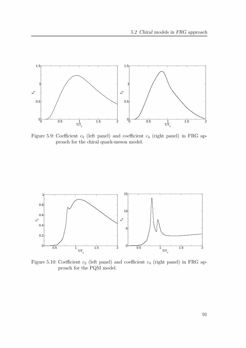
5.2 Chiral models in FRG approach
0 0.5 1 1.5 2T/Tc
0
0.5
1
1.5
c 2
0 0.5 1 1.5 2T/Tc
0
0.5
1
1.5
c 4
Figure 5.9: Coefficient c2 (left panel) and coefficient c4 (right panel) in FRG ap-proach for the chiral quark-meson model.
0.5 1 1.5 2T/Tc
0
0.2
0.4
0.6
0.8
1
c 2
0.5 1 1.5 2T/Tc
0
5
10
15
c 4
Figure 5.10: Coefficient c2 (left panel) and coefficient c4 (right panel) in FRG ap-proach for the PQM model.
91

5 Thermodynamics of hot and dense matter
quark fluctuations and consequently influences the low temperature behavior of thesecond and fourth order coefficient. Thus, in the chirally broken phase, there is astrong suppression of the quark fluctuations due to their coupling to the Polyakovloop. This is because, as already observed under mean field dynamics, the Polyakovloop suppresses the contributions of single and double quark modes to the thermo-dynamic potential. Second, similarly as in the case of the order parameter 〈σ〉 (cf.Fig. 5.8) there is a remnant of the deconfinement transition seen as a small peak atT = Tdec. Still, the quantum fluctuations in the chiral quark-meson model, with andwithout Polyakov loops clearly preserve the essential, low temperature behavior ofc2 and c4.
As in the mean field case we also investigate the behavior of the R4,2 ratios de-fined as the kurtosis in Eq. (5.26). The low temperature behavior of kurtosis asthe measure of the quark content of the leading particles carrying baryon number ispreserved within the FRG scheme. At low temperature, the kurtosis in the FRG-PQM model equals R4,2 = 9, in agreement with the LGT and hadron resonance gasmodel results [80, 45]. In the absence of the Polyakov loop in the flow equation, theone- instead of three- quark states dominate the thermodynamics at low tempera-ture. Consequently, in the FRG-QM model R4,2 = 1 is obtained instead of 9. Fromthe above discussion it is clear that the interactions of quarks with the backgroundPolyakov loop are essential to correctly reproduce the asymptotic behaviors of theR4,2 found in the LGT calculations.
At high temperature, due to finite cutoff effects (ΛUV = 1.2 GeV) the ratio R4,2
calculated in the chiral quark-meson model and PQM model does not converge tothe expected ideal gas value, where R4,2 = 6/π2. The strong suppression of c4 at hightemperature due to the finite cutoff seen in Fig. 5.9-right implies large deviations ofR4,2 from its asymptotic, ideal gas value. The cutoff actually also affects the criticalregion and leads in the FRG approach to the shift of the peak position of c4 towardsT < Tc. This behavior is also seen in Fig. 5.9-left.
A characteristic feature of the FRG-PQM model is a remnant of the deconfinementtransition that appears as a peak in the chiral susceptibility and the higher ordermoments of quark fluctuations. Such a behavior is also seen in Fig. 5.11-right inthe R4,2 ratio. The basic property of kurtosis as a measure of the net quark contentof the baryon number carrying effective degrees of freedom is clearly related toeither confinement or “statistical confinement“. However, the pion mass dependenceand increase of R4,2 near Tc when approaching the chiral limit is quantitativelyconsistent with O(4) scaling [102]. In the FRG-PQM model, the observed splittingof the ”deconfinement” and ”chiral” peak in R4,2 may be a consequence of theparticular truncation of the effective action in Eq. (5.45) and the fact that in theactual calculations Tdec < Tc by construction. Nevertheless, the enhancement of thekurtosis in the critical region could be of physical importance indicating that thelattice results for the kurtosis in the critical region are due to the combination ofconfinement and chiral dynamics. Clearly, it would be very interesting to implement
92

5.2 Chiral models in FRG approach
0.5 1 1.5 2T/Tc
0
0.5
1
1.5
R4,2
0.5 1 1.5T/Tc
0
5
10
15
20
R4,2
Figure 5.11: The kurtosis R4,2 calculated within FRG scheme in the quark-mesonmodel (left panel) and in the Polyakov loop extended quark-mesonmodel (right panel).
the RG scheme such that it includes also fluctuations of the Polyakov loop. Thiswould allow us to explore the relation between the confinement and chiral transitionwithin the PQM model and study their contributions to the relative net quarknumber fluctuations in the critical region.
We will finish our FRG treatment of the PQM model by studying the corre-sponding phase diagram, which is shown for a physical pion mass in Fig. 5.12-left.Comparing the mean field results obtained previously with the RG results shown inFig. 5.12-left it is clear that there is a significant shift in the position of the CEPtowards smaller temperatures and higher chemical potential due to fluctuations. Inthe mean field approximation we located the CEP at Tc = 163 MeV and µc = 164MeV whereas in our RG studies we find Tc = 98 MeV and µc = 307 MeV. To locatethe position of the CEP in the phase diagram, we have applied the same procedureas in the mean field case. The change of fluctuations at finite chemical potentialalong the chiral boundary line has been calculated using the Taylor expansion (5.19)around µ = µc. Then, the c2(Tc) is a measure of the net quark number fluctuationsat finite critical chemical potential. In Fig. 5.12-right we show the inverse c2 alongthe crossover line obtained in the FRG framework. There is a clear decrease of 1/c2with increasing µ. The value of µ = µc where 1/c2 → 0, as in the mean field case,indicates the position of the CEP. Also, there is a clear shift in the position of the chi-ral boundary to higher temperatures due to quantum fluctuations. Such a behaviorwas also observed in the chiral quark-meson model within the FRG approach [59].
93

5 Thermodynamics of hot and dense matter
0 100 200 300 400µ [MeV]
0
50
100
150
200
250T
[MeV
]
crossoverCEP
306 306.2 306.4 306.6µ [MeV]
0
2
4
6
8
10
12
1/c2×10-4
Figure 5.12: The phase diagram of the PQM model in FRG approach with the CEPlocated at (Tc, µc) = (98, 307) MeV (left panel) and inverse of the coef-ficient c2 along the crossover line in the vicinity of CEP (right panel).
5.2.1 Linking with QCD
In the previous section we have analyzed several thermodynamic observables withthe FRG formalism. Despite the fact that by using the RG technique one can includealso meson loops (i.e. take into account quantum fluctuations), there is a significantdrawback that plagues the FRG calculations. The inevitable introduction of an UVcutoff ΛUV , where the initial conditions for the flow equations are given, affects thehigh temperature physics6.
In order to obtain more realistic results within the RG approach, one has to care-fully choose the right value for the UV cutoff ΛUV . This choice can depend on thephysics or the temperature region one wants to investigate. Hence, there is sometemperature beyond which one cannot trust the RG results anymore. In this regionthe UV cutoff ΛUV suppresses high momenta, which in turn influences observablesthat are calculated within RG approach. What happens in the high temperatureregion, we have already seen in Fig. 5.9. Various thermodynamic quantities decreaseat high temperatures (they do not converge to the Stefan-Boltzmann limits). Thecoefficient c2 obtained from the pressure, also shows this behavior. The RG calcu-lations lead to a strong suppression of fluctuations just above the chiral transitiondue to the UV cutoff which is set to ΛUV = 1.2 GeV. Thus, removing the cutoff ΛUV
and matching the low energy theory with the high temperature region is a highlynon-trivial task.
Now we extend the flow equation for the grand canonical potential Ω(T, µ) given
6The matter concerning the cutoff effect is a subtle issue. Still, the choice of an effective fieldtheory can also have a considerable influence on the high (or low) energy physics. The chiralquark-meson model is a low energy model and lacks gauge degrees of freedom. This can alsobe a reason for obtaining results that deviate from LGT calculations.
94

5.2 Chiral models in FRG approach
by Eq. (5.45) in order to approach the high energy sector of QCD. The idea is toadd to Eq. (5.45) a flow equation for the high-energy degrees of freedom. A firstattempt in this direction has been made in Ref. [46]. According to LGT [50, 51] theequation of state of an interacting system has the properties of a free gas at hightemperatures (T ≥ 200 MeV). Thus, one can neglect the full gauge interactions ofthe high energy QCD and approximate the corresponding system with a free gasof quarks and gluons at some scale k > ΛUV . The advantage of using this sort ofan approximation is to remove the cutoff ΛUV which is inevitably present duringintegration of Eq. (5.45).
We start with the flow equation without Polyakov loops for several reasons. First,by using the set of optimized regulators we can integrate the existing flow equationfor chiral quark-meson model for the high-energy degrees of freedom analytically.The second point is that we are interested only in the high-energy part of the flowi.e. for k > ΛUV . For the energy scale k < ΛUV we will switch again to Eq. (5.45).Here we use a simplified model of a gas of massless quarks and gluons to link thehigh-energy degrees of freedom with the chiral low-energy part.
We again use the optimized cutoff functions and neglect the current quark massfor the two light flavors. The flow equation for the high-energy part has then thefollowing form
∂kΩUVk (T, µ) =
k3
12π2
[
16
(
1 + 2nB(k)
)
− 2νq
(
1 − nF (k) − nF (k)
)]
. (5.49)
In order to link the effective chiral quark-meson model with high-energy degreesof freedom we shall adapt the idea introduced in Ref. [46] and proceed as follows.First, we integrate Eq. (5.49) starting with some cutoff Λ∞ which can be placedat infinity, to ΛUV which is the cutoff used for integrating flow equation (5.45) orits simplified form with no Polyakov loop. At the scale k = ΛUV we switch toEq. (5.45) or its analogue without Polyakov loop and integrate the remaining flowequation down to k = 0. In this way one has a smooth transition from the highenergy part of the theory to the chiral low-energy part. The main goal we aim forin this approximation is to remove the dependence on the cutoff ΛUV . This is easyto achieve due to the simple form of Eq. (5.49) which allows an analytic integrationstarting from infinity.
The integration of Eq. (5.49) yields
ΩUV (T, µ) =1
6π2
(16NB + 12NF − 12NF
)∣∣∣∣
ΛUV
∞
(5.50)
95

5 Thermodynamics of hot and dense matter
where the following functions have been introduced
NB =k4
8− k3TLi1[e
−k/T ] − 3k2T 2Li2[e−k/T ]
−6kT 3Li3[e−k/T ] − 6T 4Li4[e
−k/T ], (5.51a)
NF =k4
8− k3TLi1[e
−(k−µ)/T ] − 3k2T 2Li2[e−(k−µ)/T ]
−6kT 3Li3[e−(k−µ)/T ] − 6T 4Li4[e
−(k−µ)/T ], (5.51b)
NF =k4
8− k3TLi1[−e−(k+µ)/T ] − 3k2T 2Li2[−e−(k+µ)/T ]
−6kT 3Li3[−e−(k+µ)/T ] − 6T 4Li4[−e−(k+µ)/T ], (5.51c)
and Lin[z] are the polylogarithmic functions given in Appendix B. The arguments ofthe polylogarithm functions in Eqs. (5.51a), (5.51b) and (5.51c) represent the clas-sical Maxwell-Boltzmann distribution functions for gluons, quarks and antiquarksrespectively. Using the feature that the polylogarithmic function vanishes at zero,Eq. (5.50) can further be calculated by substituting the limits of integration. Obvi-ously, a divergent part in Eq. (5.50) will nevertheless remain. However, the vacuumpart can also be easily calculated
ΩUVvac (T, µ) =
8
3π2
(Λ4UV
8− Λ4
∞
8
)
. (5.52)
Knowing that the finite temperature part of the pressure does not depend on thevacuum energy, we can extract the high-energy contribution to the pressure, sincethe regularized divergent part of the potential drops out [46]. This high-energycontribution we then add to the one obtained from the RG calculation. We showour results in Fig. 5.13.
There is now a smooth transition of fluctuations from the high- to the chiral,low-energy part of the theory. Also for high temperatures we observe that both, c2and c4 approach to their ideal gas value. This has not been the case where thesecoefficients have been calculated only within a RG method, due to a finite UV cutoff.
5.3 Conclusions
In this chapter we have investigated some thermodynamic properties as well as thephase structure of hot and dense matter. As a tool, we used both, the mean fieldapproximation and the FRG approach. The effective model we have used was thePQM model. In order to exhibit the importance of gluonic degrees of freedom, wealso used the chiral quark-meson model and compared the results obtained with thismodel with the ones where gluon dynamics is included via the Polyakov loop.
96

5.3 Conclusions
0 0.5 1 1.5 2T/Tc
0
0.5
1
1.5
2
c 2
0 0.5 1 1.5 2T/Tc
0
0.5
1
1.5
2
c 4
Figure 5.13: Taylor expansion coefficient c2 (left panel) and c4 (right panel) for thechiral quark-meson model calculated in the FRG approach with a cutoffΛUV (solid line) and after removing the cutoff by the inclusion of anadditional flow for a free gas of quarks and gluons (dashed line).
The mean field investigation of the PQM model started with the exploration ofthe temperature dependence of the Polyakov loop at vanishing chemical potential µ.We used this behavior to determine the deconfinement transition temperature. Thistemperature was obtained by calculating the temperature derivative of the Polyakovloop. The position of the peak marks the deconfinement transition.
The next subject we addressed was the in-medium meson masses and the con-stituent quark mass. We have studied their behavior also at µ = 0. Subsequentto this study, we have applied the Taylor expansion method of the pressure forvanishing µ. The reason for this was twofold. First, we wanted to emphasize theimportance of gluonic degrees of freedom. Second, we used this expansion in thestudy of further thermodynamic observables that have proven to be valuable probesof deconfinement and chiral dynamics. We have extracted the expansion coefficientsc2 and c4 and showed their temperature dependence. In the case where no gluonicbackground is present (chiral quark-meson model) we see, as expected, the absenceof suppression of quark degrees of freedom at low temperatures. On the other hand,after calculating coefficient c2 for the PQM model, the suppression in the low tem-perature region is present.
In the first part of the chapter, the focus of our study was also on the propertiesof the kurtosis R4,2 of net quark number fluctuations and the dimensionless inversecompressibility Rκ. We have studied the behavior of these observables near thechiral transition as functions of the pion mass. We showed that it is necessary toinclude the coupling of the quarks to the Polyakov loop, in order to reproduce thelow-temperature behavior of the kurtosis expected in QCD. We also demonstratedthat near the pseudocritical temperature, both these observables are very sensitive
97

5 Thermodynamics of hot and dense matter
to the pion mass. For the physical value of mπ, the kurtosis develops a peak and theinverse compressibility a dip at the pseudocritical temperature. These structuresdisappear for large mπ. Our results supports the notion that, for physical quarkmasses, the strange quark decouples from the critical fluctuations and the scalingproperties are governed by O(4), the expected universality class of two flavor QCD.We also found a suppression of Rκ, as the critical end point CEP is approached.However, Rκ remains finite at the CEP, if the Taylor expansion in µ/T of thethermodynamic pressure is used.
Furthermore, we also explored the phase diagram of the PQM model, for thephysical pion mass. Exploring the behavior of the coefficient c2 along the crossoverline, we located the position of the CEP. We calculated the inverse of c2 along thecrossover line from the Taylor expansion of the pressure, but now, at finite valuesof chemical potential µ. Consequently, as c2 is related to the fluctuations of thenet quark number, we observed a rapid decrease of the inverse of c2 as the CEP isapproached.
In the second part, we applied the FRG method to the chiral quark-meson modelas well as to the PQM model. We have discussed different thermodynamic prop-erties of the PQM model including quantum fluctuations within FRG method. Inorder to do so, we have introduced a suitable truncation of the PQM model that al-lowed us to extend the previous RG based studies of the chiral quark-meson model.This truncation consists of introducing a coupling of fermions to Polyakov loops.We have derived and subsequently solved the flow equation for the scale depen-dent thermodynamic potential at finite temperature and density in the presence ofa background gluonic field. In our studies of thermodynamics we have discussedthe role of fluctuations on the critical properties of the model. We have shownthat the non-perturbative dynamics introduced within the FRG method modifiesthe phase diagram leading to a shift in the position of the CEP towards lower tem-perature. Furthermore, following the investigations in the mean field approximationwe have again, now within the FRG method, analyzed the fluctuations of the netquark number density and the ratio of its fourth to second order cumulant moments(kurtosis). A comparison of the FRG approach with and without gluon backgroundfield was performed. We have shown that the FRG extended quark-meson modelpreserves basic properties of kurtosis obtained in the LGT calculations only if thePolyakov loop is included in the flow equation. Thus, the extension of the FRGmethod proposed here, that accounts for couplings of fermions to background gluonfields is of particular relevance if the quark-meson model is considered as an effectivedescription of the QCD thermodynamics near the phase transition.
Finally, the influence of the ultraviolet cutoff effects on the thermodynamics withinthe FRG approach was also discussed. By means of a simple model that is repre-sented as a free gas of massless quarks and gluons, we have introduced an additionalflow equation for the high-energy degrees of freedom. Within this approximationwe have undertaken a full RG study of the coefficients c2 and c4 for the chiral
98

5.3 Conclusions
quark-meson model. The results are in excellent agreement with the correspondingStefan-Boltzmann limits in the high temperature region. The cutoff effect has beensuccessfully removed, and the Taylor expansion coefficients approach their expectedideal gas values.
99

100

Chapter 6
Summary and outlook
In this thesis the main subject of investigation was the behavior of matter underextreme conditions, i.e. hot and dense matter. We have used two effective theorymodels (the chiral quark-meson model and the Polyakov quark-meson model) inorder to assess various thermodynamic properties as well as the critical behavior ofQCD at nonvanishing temperature and chemical potential. In order to obtain ourresults, we have used the aforementioned models as a low-energy realization of QCD.In the low-energy region QCD is highly nonperturbative (i.e. calculation based onperturbation theory fail). As a tool for performing the calculations we have employedthe functional renormalization group approach to assess the role of fluctuations.Besides the RG approach, we have also used the mean field approximation. TheRG approach has proven to be useful in investigating the scaling behavior of thechiral quark-meson model, whereas both, the RG and mean field calculations havebeen used in exploring various thermodynamic properties, the phase diagram andthe phase structure of the chiral quark-meson and the PQM model. Apart fromcomparing the results that have been obtained within these two different approaches,we have also investigated the effects of including or excluding certain degrees offreedom present in the models. In this way we have put emphasis on the gluonicdegrees of freedom and their contribution to QCD thermodynamics. The importanceof having a gluonic background in effective QCD-inspired model is highlighted byour results obtained both, in the mean field as well as in the RG approach. Wehave also obtained the corresponding phase diagrams for both models, calculatedfor physical pion masses. In each case we have also located the critical endpoint atthe end of the crossover line.
101

6 Summary and outlook
Summary
In the first chapter of this thesis we have given a short motivation for our study.What followed, was Chapter 2 where some basic concepts regarding (non)-Abeliangauge theories were introduced and explained. Here, we avoided going into de-tails (especially into subtle mathematical details concerning functional methods andgroup theory, since they are not of crucial importance in our work) and rather triedto give an overall picture of gauge theories and especially the strong interaction. Fur-ther, in this chapter we have also introduced models used in our studies, namely thechiral quark-meson model and its extension, the Polyakov quark-meson model. Forboth models we have given the Lagrangians and discussed the main features. In theend, the basic concepts of chiral symmetry breaking and confinement/deconfinementwere introduced and discussed.
The renormalization group approach was introduced in Chapter 3. In the first partof Chapter 3, the motivation for using the RG method was given. This particulartheoretical method was the main tool in the calculations, where we explored thecritical properties and the scaling behavior of the chiral quark-meson model. At thebeginning of Chapter 3, we introduced the main ideas of the RG approach. Next,we also discussed the most important features of the RG and briefly discussed theproblems where this method has already been successfully applied.
The focus of this presentation were the critical phenomena, as the most prominentexample of the success of the RG approach in physics. Later, in the subsequentsection of Chapter 3, we focused on one special RG approach, namely the functionalrenormalization group (FRG) approach. Before giving the main characteristics ofthe FRG, we also introduced the basic concepts of some important objects thatappear in quantum field theory and statistical physics. The notions of the generatingfunctional of the n-point correlation functions, (dis)connected Green functions andfinally, the effective action have been introduced and briefly explained. The mostimportant part, the flow equation for the effective average action was derived. Wealso discussed the most important features and properties of the flow equation, thatwas the starting point in all our RG investigation at nonvanishing temperature andchemical potential.
In Chapter 4 we employed the FRG method in order to explore the critical prop-erties of the chiral-quark meson model and the O(4) scaling. As a starting pointfor our study we used the flow equation for the scale dependent thermodynamicpotential at finite temperature and density, which we derived in the presence of asymmetry-breaking external field. The main focus of our study was the universalscaling behavior of various physical quantities that are sensitive to the chiral phasetransition.
We also analyzed the leading scaling behavior of the longitudinal and transversesusceptibilities as well as their ratios. In this case, the critical point was approachedfrom the side of the symmetric and the broken phase for small, but finite values of the
102

external field. The notion of effective critical exponents was defined and connectedwith the calculated ratios of some physical quantities. The values of the critical ex-ponents that were extracted, directly through logarithmic fits and indirectly throughdifferent ratios of corresponding observables, confirm the expectations that the chi-ral phase transition of the 2-flavor effective chiral quark-meson model belongs to theO(4) universality class.
In Chapter 5 we considered the chiral quark-meson model and the PQM modelalso for finite values of the chemical potential. The first part of the analysis was donein the mean field approximation. Subjects of our study was different thermodynamicproperties as well as the phase structure of these models. Here, we have focused onthe behavior of the kurtosis R4,2 of the net quark number fluctuations and the di-mensionless inverse compressibility Rκ near the chiral transition as functions of thepion mass. In all these calculations, we have employed the Taylor expansion of thepressure and also extracted the expansion coefficients c2 and c4. By observing howthese coefficients behave as functions of temperature T , we demonstrated the impor-tance of gluonic degrees of freedom in the model. Using the same Taylor expansion,but now expanding the pressure around the non zero (critical) chemical potential,we have calculated the coefficient c2 along the crossover line. The coefficient c2 isrelated to fluctuations of net quark number and consequently, this method has beenused to locate the position of the critical endpoint in the phase diagram.
In the second part of Chapter 5, the PQM model was analyzed within the FRGapproach. Still, the Polyakov loop variable was treated on the mean field level. Wehave again in our calculations used the Taylor expansion of the pressure to calculatecoefficients the c2 and c4. First, all calculations have been done for the chiral quark-meson model. Later, we have included Polyakov loops in order to explore the effectof having gluonic degrees of freedom in the model. As in the mean field case,we showed the corresponding phase diagram with the critical endpoint, that wasdetermined in the same way as in the mean field approximation.
In the end we have also addressed the issue of the cutoff effect. This effect is alwayspresent in RG calculations, and here we used a simplified model to alleviate thisproblem. A further flow equation for the thermodynamic potential was introduced inorder to link the chiral quark-meson model with the high energy sector of QCD [46].The full gauge interactions of the high energy sector of QCD were neglected. As aconsequence, the system in this regime was approximated by a free gas of quarks andgluons. We showed in the case of the coefficients c2 and c4 for the chiral quark-mesonmodel how the cutoff effect can be reduced. This was achieved by integrating theflow equation for a free gas of quarks and gluons from infinity to the cutoff ΛUV andthen we have switched to the flow equation for the chiral quark-meson model usedin our previous calculations. In this way we obtained for both coefficients c2 andc4 a smooth transition from the low energy (chiral) to the high energy part of thetheory. Moreover, the cutoff effect was to a large extent removed and c2 and c4 showa nice convergence to the corresponding ideal gas values in the high temperature
103

6 Summary and outlook
limit.
Outlook
There are several possible extensions of the work and results presented in this thesis.First, regarding the mean field analysis, one could extend the results presented hereby an exact mean field calculation of the dimensionless inverse compressibility Rκ.Due to the Taylor expansion, the value of Rκ is finite even as the CEP is approached.This however should not be the case, since it is expected that Rκ goes to zero. TheTaylor expansion used in this work is however good enough to estimate the valueof Rκ but not adequate to identify the exact location of the CEP. Thus, we expectthat an exact calculation of the dimensionless inverse compressibility must give zerovalue for Rκ at the CEP. This calculation would then underpin the claim that thevanishing of Rκ should be treated as a signal that the CEP has been approached.
In respect of different approaches and methods used to locate the CEP (theoreti-cally and experimentally) one particular idea has attracted a lot of attention in theheavy-ion community. It has been proposed that the so called focusing of the isen-tropic lines in the QCD phase diagram could indicate the position of the CEP [103].This means that the CEP should act as an attractor for isentropic lines in hot anddense matter. Studies done recently within the mean field approximation, show thatno strong focusing behavior exists near the CEP [104]. Preliminary results obtainedin the mean field approximation as well as in the RG approach confirm these re-sults [105]. Even if fluctuations are included, no focusing behavior is observed. Weconclude that focusing towards the CEP is not a universal phenomenon. The workon this subject is still in progress, and the results are not presented in this thesis.
We have also addressed another subject concerning the RG treatment, namely thecutoff effect. It would be interesting to investigate this subtle issue as well as the oneconcerning the connection between a mean field approximation and a RG approach.In which limit is an RG calculation equivalent to a mean field approximation? Is aUV cutoff in a mean field calculation (for the chiral quark-meson model, where theDirac see has been neglected, cf. Chapter 2) equivalent to the RG cutoff? Some ofthese issues are addressed in our recent work [105] that is still in progress.
One of the most challenging and interesting extensions of this work would betowards a full RG treatment of the PQM model. In this thesis, the Polyakov loopvariable was studied only in the mean field approximation. A full RG treatment ofthe Polyakov loop would yield results beyond the usual mean field analysis, since allfluctuations would then be taken into account. In this work we have gone one stepbeyond the mean field analysis of the PQM model, by coupling the Polyakov loopwith quarks within a truncation scheme that is then suitable for a FRG treatment.What is missing in the present approach is the RG flow of the Polyakov loop whichwould include all fluctuations and would consequently allow a full RG treatment of
104

the PQM model. In the end, in order to obtain a model that could be extendedtowards full QCD one would also need to include the whole gauge dynamics. It isplausible that such a full RG analysis would yield results that could give a valuableinput to further theoretical and experimental studies of hot and dense QCD matter.This would bring us, at least one step, closer to the understanding of the nature ofQCD phase transition(s).
105

106

Appendix A
Notations and conventions
Throughout this thesis we work in Euclidean spacetime. For the standard Diracgamma matrices we have
γµ, γν = −2δµν . (A.1)
Their standard representation is given by
γ0 =
(i 00 −i
)
, γj =
(0 −σjσj 0
)
, γ5 =
(0 −1−1 0
)
, (A.2)
where σj are the Pauli matrices
σ1 =
(0 11 0
)
, σ2 =
(0 −ii 0
)
, σ3 =
(1 00 −1
)
. (A.3)
107

108

Appendix B
Temperature limits
In this Appendix we investigate more closely the temperature limits of the fermioniccontribution to the pressure of the system. We also provide a bit more detailsconcerning derivation of Eqs. (5.24) and (5.31).
Low-temperature limit
In the low-temperature limit one has ℓ, ℓ∗ → 0, which implies the suppression of theone- and two-quark states. The pressure of a system P (T, µ) is related to the grandcanonical potential Ω(T, µ) by
P (T, µ) = −Ω(T, µ)
V. (B.1)
Now, using Eq. (5.14) the fermion contribution to the pressure is of the form
Pqq =NfT
π2
∞∫
0
dp p2(ln[1 + e−3(Ep−µ)/T ] + ln[1 + e−3(Ep+µ)/T ]
). (B.2)
This expression can be brought in other form after integration by parts and reads
Pqq =NfT
π2
∞∫
0
dpp4
Ep
(1
e3(Ep−µ)/T+
1
e3(Ep+µ)/T
)
. (B.3)
The next step is to change the variable x = Ep/mq that transforms (B.3) as follows
Pqq =NfT
π2
∞∫
1
dxm4q
(x2 − 1
) 3
2
(1
e3(mqx−µ)/T + 1+
1
e3(mqx+µ)/T + 1
)
. (B.4)
109

B Temperature limits
In order to solve the integrals present in (B.4) we have to use the Boltzmann ap-proximation, that is valid if 3mq/T > 1. Thus, in this approximation the fermionicpart of the pressure is
Pqq ≃NfT
π2
∞∫
1
dxm4q
(x2 − 1
) 3
2
(e−3(mqx−µ)/T + e−3(mqx+µ)/T
). (B.5)
At this point we have to make a small, but inevitably mathematical detour byintroducing the modified Bessel function of the second kind Kn(z) that satisfiesvarious identities1. We will make use of the following identity
Kn(z) =
√π
(n− 1
2
)!
(z
2
)n∞∫
1
dx (x2 − 1)n−1
2 e−zx. (B.6)
Now, we can represent the fermionic pressure in the low-temperature region, in theBoltzmann approximation with
Pqq(T, µ)
T 4=
2Nf
27π2
(3mq
T
)2
K2
(3mq
T
)
cosh3µ
T, (B.7)
that is nothing but Eq. (5.31).
High-temperature limit
As in the low-temperature case, we start with Eq. (5.14) that for ℓ, ℓ∗ → 1 reducesto
Ωqq
V= −Pqq = −2NcNfT
∫d3p
(2π)3
(ln[1 + e−(Ep−µ)/T ] + ln[1 + e−(Ep+µ)/T ]
). (B.8)
Further integration by parts that can be done in the same way as in the low tem-perature limit, yields for the pressure
Pqq = 2NcNfT1
6π2
∞∫
0
dpp4
Ep(nF (Ep) + nF (Ep)) , (B.9)
1By definition, modified Bessel functions of the second kind represent one of the solution to themodified Bessel differential equation
z2 d2y
dz2+ z
dy
dz− (z2 + n2)y = 0.
110

where nF (Ep) and nF (Ep) are fermionic distribution functions and Ep =√~p 2 +m2
q
is the quark energy. In the case of a massless free quark/antiquark gas (mq → 0),the expression for the pressure simplifies considerably, and reads
Pqq = 2NcNf1
6π2
∞∫
0
dp p3
(1
e(p−µ/)T + 1+
1
e(p+µ/)T + 1
)
. (B.10)
Finally, the integrals appearing in (B.10) can be integrated analytically yielding
Pqq = 2NcNf1
6π2(−6T 4)
(Li4(−eµ/T ) + Li4(−e−µ/T )
). (B.11)
With Lin(z) we have defined the polylogarithm function that is also known as deJonquiere’s function. In a complex plane z it is defined through the following sum
Lin(z) =
∞∑
k=1
zk
kn. (B.12)
The integral representation of the polylogarithm function is given by
Lin+1(z) =
z∫
0
Lin(t)
tdt. (B.13)
For negative integer values of n the polylogarithm function Lin(z) can be expressedas a ratio of polynomials. The polylogarithm functions in (B.11) are given by
Li4(−eµ/T ) + Li4(−e−µ/T ) = −7π4
360− π2
12
(µ
T
)2
− 1
24
(µ
T
)4
, (B.14)
and plugging this result back into (B.11) finally gives Eq. (5.24)
Pqq(T, µ)
T 4= NfNc
[1
12π2
(µ
T
)4
+1
6
(µ
T
)2
+7π2
180
]
. (B.15)
111

112

Bibliography
[1] K. Yagi, T. Hatsuda, Y. Miake, Quark-Gluon Plasma: From Big Bang to LittleBang, (Cambridge University Press, Cambridge, England, 2005).
[2] P. de Forcrand, S. Kim and O. Philipsen, A QCD chiral critical point at smallchemical potential: is it there or not?, PoS LAT2007, 178 (2007).
[3] http://www.star.bnl.gov/public/imagelib/collisions2001/ev2 front.jpg.
[4] H. Meyer-Ortmanns, Phase transitions in quantum chromodynamics, Rev. Mod.Phys. 68, 473 (1996).
[5] http://www.gsi.de/fair/overview/research/antiprotons.html.
[6] http://www.gsi.de/fair/overview/research/nuclear-matter.html
[7] M. Gell-Mann and F. E. Low, Quantum electrodynamics at small distancesPhys. Rev. 95, 1300 (1954).
[8] D. J. Gross and F. Wilczek, Ultraviolet behavior of non-Abelian gauge theories,Phys. Rev. Lett. 30, 1343 (1973).
[9] H. D. Politzer, Reliable perturbative results for strong interactions?, Phys. Rev.Lett. 30, 1346 (1973).
[10] S. Bethke, alpha(s) at Zinnowitz 2004, Nucl. Phys. Proc. Suppl. 135, 345(2004).
[11] M. Gell-Mann and M. Levy, The axial vector current in beta decay, NuovoCimento 16, 705 (1960).
113

Bibliography
[12] A. M. Polyakov, Thermal Properties Of Gauge Fields And Quark Liberation,Phys. Lett. B 72, 477 (1978).
[13] G. ’t Hooft, On The Phase Transition Towards Permanent Quark Confinement,Nucl. Phys. B 138, 1 (1978).
[14] R. D. Pisarski, Notes on the deconfining phase transition, arXiv:hep-ph/0203271.
[15] M. E. Fisher, The renormalization group in the theory of critical behavior, Rev.Mod. Phys. 46, 597 (1974).
[16] M. E. Fisher, Renormalization group theory: Its basis and formulation in sta-tistical physics, Rev. Mod. Phys. 70, 653 (1998).
[17] S. K. Ma, Introduction to the renormalization group, Rev. Mod. Phys. 45, 589(1973).
[18] M. Cheng et al., QCD equation of state with almost physical quark masses,Phys. Rev. D 77, 014511 (2008).
[19] Y. Aoki, Z. Fodor, S. D. Katz and K. K. Szabo, The QCD transition tempera-ture: Results with physical masses in the continuum limit, Phys. Lett. B 643,46 (2006).
[20] A. Gocksch and M. Ogilvie, Finite temperature deconfinement and chiral sym-metry restoration at strong coupling, Phys. Rev. D 31, 877 (1985).
[21] M. Buballa, NJL model analysis of quark matter at large density, Phys. Rept.407, 205 (2005).
[22] P. N. Meisinger and M. C. Ogilvie, Chiral symmetry restoration and ZN sym-metry, Phys. Lett. B 379, 163 (1996).
[23] P. N. Meisinger, T. R. Miller and M. C. Ogilvie, Phenomenological equationsof state for the quark-gluon plasma, Phys. Rev. D 65, 034009 (2002).
[24] K. Fukushima, Chiral effective model with the Polyakov loop, Phys. Lett. B 591,277 (2004).
[25] F. Sannino, Polyakov loops versus hadronic states, Phys. Rev. D 66, 034013(2002).
[26] A. Mocsy, F. Sannino and K. Tuominen, Confinement versus chiral symmetry,Phys. Rev. Lett. 92, 182302 (2004).
114

Bibliography
[27] C. Ratti, M. A. Thaler and W. Weise, Phases of QCD: Lattice thermodynamicsand a field theoretical model, Phys. Rev. D 73, 014019 (2006).
[28] S. Digal, E. Laermann and H. Satz, Deconfinement through chiral symmetryrestoration in two-flavour QCD, Eur. Phys. J. C 18, 583 (2001).
[29] E. Megias, E. Ruiz Arriola and L. L. Salcedo, Polyakov loop in chiral quarkmodels at finite temperature, Phys. Rev. D 74, 065005 (2006).
[30] E. M. Ilgenfritz and J. Kripfganz, Dynamical fermions at nonzero chemicalpotential and temperature: Mean field approach, Z. Phys. C 29, 79 (1985).
[31] K. Fukushima, Effects of chiral restoration on the behaviour of the Polyakovloop at strong coupling, Phys. Lett. B 553, 38 (2003).
[32] K. Fukushima, Relation between the Polyakov loop and the chiral order param-eter at strong coupling, Phys. Rev. D 68, 045004 (2003).
[33] B. J. Schaefer, J. M. Pawlowski and J. Wambach, The phase structure of thePolyakov-quark-meson model, Phys. Rev. D 76, 074023 (2007).
[34] C. Wetterich, Average action and the renormalization group equations, Nucl.Phys. B 352, 529 (1991).
[35] N. Tetradis and C. Wetterich, Scale dependence of the average potential aroundthe maximum in Phi**4 theories, Nucl. Phys. B 383, 197 (1992).
[36] C. Wetterich, Exact evolution equation for the effective potential, Phys. Lett. B301, 90 (1993).
[37] T. R. Morris, The exact renormalization group and approximate solutions, Int.J. Mod. Phys. A 9, 2411 (1994).
[38] U. Ellwanger, Flow equations for N point functions and bound states, Z. Phys.C 62, 503 (1994).
[39] J. Berges, N. Tetradis and C. Wetterich, Non-perturbative renormalization flowin quantum field theory and statistical physics, Phys. Rept. 363, 223 (2002).
[40] H. Gies, Introduction to the functional RG and applications to gauge theories,arXiv:hep-ph/0611146.
[41] B. Delamotte, An introduction to the nonperturbative renormalization group,arXiv:cond-mat/0702365.
[42] C. Sasaki, B. Friman and K. Redlich, Susceptibilities and the phase structureof a chiral model with Polyakov loops, Phys. Rev. D 75, 074013 (2007).
115

Bibliography
[43] C. Ratti, S. Roessner, M. A. Thaler and W. Weise, Thermodynamics of thePNJL model, Eur. Phys. J. C 49, 213 (2007).
[44] S. K. Ghosh, T. K. Mukherjee, M. G. Mustafa and R. Ray, Susceptibilities andspeed of sound from PNJL model, Phys. Rev. D 73, 114007 (2006).
[45] S. Ejiri, F. Karsch and K. Redlich, Hadronic fluctuations at the QCD phasetransition, Phys. Lett. B 633, 275 (2006).
[46] J. Braun, K. Schwenzer and H. J. Pirner, Linking the quark meson model withQCD at high temperature, Phys. Rev. D 70, 085016 (2004).
[47] D. F. Litim, Optimized renormalization group flows, Phys. Rev. D 64, 105007(2001).
[48] B. Stokic, B. Friman and K. Redlich, The functional renormalization groupmethod and O(4) scaling, (to be submitted to Phys. Rev. D).
[49] B. Stokic, B. Friman and K. Redlich, Quantum fluctuations and the thermody-namics of the Polyakov loop extended quark-meson model, (to be submitted toPhys. Rev. D).
[50] G. Boyd, J. Engels, F. Karsch, E. Laermann, C. Legeland, M. Lutgemeier andB. Petersson, Thermodynamics of SU(3) Lattice Gauge Theory, Nucl. Phys. B469, 419 (1996).
[51] F. Karsch, E. Laermann and A. Peikert, The pressure in 2, 2+1 and 3 flavourQCD, Phys. Lett. B 478, 447 (2000).
[52] R. D. Pisarski and F. Wilczek, Remarks on the chiral phase transition in chro-modynamics, Phys. Rev. D 29, 338 (1984).
[53] K. Rajagopal and F. Wilczek, Static and dynamic critical phenomena at asecond order QCD phase transition, Nucl. Phys. B 399, 395 (1993).
[54] F. Parisen Toldin, A. Pelissetto and E. Vicari, The 3-D O(4) universality classand the phase transition in two-flavor QCD, JHEP 0307, 029 (2003).
[55] J. Engels, S. Holtmann, T. Mendes and T. Schulze, Finite size scaling functionsfor 3-d O(4) and O(2) spin models and QCD, Phys. Lett. B 514, 299 (2001).
[56] J. Engels and T. Mendes, Goldstone mode effects and scaling function for thethree-dimensional O(4) model, Nucl. Phys. B 572, 289 (2000).
[57] J. Engels, L. Fromme and M. Seniuch, Correlation lengths and scaling functionsin the three-dimensional O(4) model, Nucl. Phys. B 675, 533 (2003).
116

Bibliography
[58] S. Roessner, C. Ratti and W. Weise, Polyakov loop, diquarks and the two-flavourphase diagram, Phys. Rev. D 75, 034007 (2007).
[59] B. J. Schaefer and J. Wambach, Susceptibilities near the QCD (tri)critical point,Phys. Rev. D 75, 085015 (2007).
[60] D. U. Jungnickel and C. Wetterich, Effective action for the chiral quark-mesonmodel, Phys. Rev. D 53, 5142 (1996).
[61] J. Berges, D. U. Jungnickel and C. Wetterich, Two flavor chiral phase transitionfrom nonperturbative flow equations, Phys. Rev. D 59, 034010 (1999).
[62] J. Berges, D. U. Jungnickel and C. Wetterich, The chiral phase transition athigh baryon density from nonperturbative flow equations, Eur. Phys. J. C 13,323 (2000).
[63] B. J. Schaefer and H. J. Pirner, The equation of state of quarks and mesons ina renormalization group flow picture, Nucl. Phys. A 660, 439 (1999).
[64] J. Meyer, G. Papp, H. J. Pirner and T. Kunihiro, Renormalization group flowequation at finite density, Phys. Rev. C 61, 035202 (2000).
[65] N. Tetradis, The quark-meson model and the phase diagram of two-flavourQCD, Nucl. Phys. A 726, 93 (2003).
[66] B. J. Schaefer and J. Wambach, The phase diagram of the quark meson model,Nucl. Phys. A 757, 479 (2005).
[67] J. Braun and B. Klein, Scaling functions for the O(4)-model in d = 3 dimen-sions, Phys. Rev. D 77, 096008 (2008).
[68] J. P. Blaizot, A. Ipp, R. Mendez-Galain and N. Wschebor, Perturbation the-ory and non-perturbative renormalization flow in scalar field theory at finitetemperature, Nucl. Phys. A 784, 376 (2007).
[69] E. K. Riedel and F. J. Wegner, Effective critical and tricritical exponents, Phys.Rev. B 9, 294 (1974).
[70] D. O’Connor and C. R. Stephens, Renormalization group theory of crossovers,Phys. Rept. 363, 425 (2002).
[71] G. Boyd, J. Fingberg, F. Karsch, L. Karkkainen and B. Petersson, Criticalexponents of the chiral transition in strong coupling QCD, Nucl. Phys. B 376,199 (1992).
[72] F. Karsch and E. Laermann, Susceptibilities, the specific heat and a cumulantin two flavor QCD, Phys. Rev. D 50, 6954 (1994).
117

Bibliography
[73] A. Kocic, J. B. Kogut and M. P. Lombardo, Universal properties of chiralsymmetry breaking, Nucl. Phys. B 398, 376 (1993).
[74] E. Berezin, D. J. Wallace and K. G. Wilson, Feynman-graph expansion for theequation of state near the critical point, Phys. Rev. B 7, 232 (1973).
[75] A. Pelissetto and E. Vicari, Critical phenomena and renormalization group the-ory, Phys. Rept. 368, 549 (2002).
[76] K. Kanaya and S. Kaya, Critical exponents of a three dimensional O(4) spinmodel, Phys. Rev. D 51, 2404 (1995).
[77] M. E. Fisher, V. Privman, First-order transitions breaking O(n) symmetry:Finite-size scaling, Phys. Rev. B 32, 447 (1985).
[78] D. J. Wallace and R. K. P. Zia, Singularities induced by Goldstone modes, Phys.Rev. B 12, 5340 (1975).
[79] R. B. Griffiths, Thermodynamic functions for fluids and ferromagnets near thecritical point, Phys. Rev. 158, 176 (1967).
[80] C. R. Allton, S. Ejiri, S. J. Hands, O. Kaczmarek, F. Karsch, E. Laermann andC. Schmidt, The equation of state for two flavor QCD at non-zero chemicalpotential, Phys. Rev. D 68, 014507 (2003).
[81] F. Karsch, S. Ejiri and K. Redlich, Hadronic fluctuations in the QGP, Nucl.Phys. A 774, 619 (2006).
[82] S. Ejiri et al., The QCD equation of state for two flavours at non-zero chemicalpotential, Nucl. Phys. A 774, 837 (2006).
[83] Z. Fodor and S. D. Katz, Lattice determination of the critical point of QCD atfinite T and µ, JHEP 0203, 014 (2002).
[84] Z. Fodor and S. D. Katz, Critical point of QCD at finite T and µ, lattice resultsfor physical quark masses, JHEP 0404, 050 (2004).
[85] M. D’Elia and M. P. Lombardo, Finite density QCD via imaginary chemicalpotential, Phys. Rev. D 67, 014505 (2003).
[86] P. de Forcrand and O. Philipsen, The QCD phase diagram for three degenerateflavors and small baryon density, Nucl. Phys. B 673, 170 (2003).
[87] R. V. Gavai and S. Gupta, Fluctuations, strangeness and quasi-quarks in heavy-ion collisions from lattice QCD, Phys. Rev. D 73, 014004 (2006).
118

Bibliography
[88] R. V. Gavai and S. Gupta, Simple patterns for non-linear susceptibilities nearT (c), Phys. Rev. D 72, 054006 (2005).
[89] R. V. Gavai and S. Gupta, Quark number susceptibilities and the Wroblewskiparameter, Eur. Phys. J. C 43, 31 (2005).
[90] F. Karsch, Recent lattice results on finite temperature and density QCD, part I,PoS CPOD07, 026 (2007).
[91] C. Schmidt [for RBC-Bielefeld Collaboration], Baryon number, strangeness andelectric charge fluctuations at zero and non-zero chemical potential, J. Phys. G35, 104093 (2008).
[92] C. Sasaki, B. Friman and K. Redlich, Quark number fluctuations in a chiralmodel at finite baryon chemical potential, Phys. Rev. D 75, 054026 (2007).
[93] C. Sasaki, B. Friman and K. Redlich, Chiral phase transition in the presence ofspinodal decomposition, Phys. Rev. D 77, 034024 (2008).
[94] C. Sasaki, B. Friman and K. Redlich, Effective chiral model with Polyakov loopsand its application to hot/dense medium, Prog. Theor. Phys. Suppl. 168, 291(2007).
[95] K. Redlich, B. Friman and C. Sasaki, QCD phase diagram and charge fluctua-tions, J. Phys. G 34, S437 (2007).
[96] See e.g. Proceedings of ”Quark Matter 2008”.
[97] M. Le Bellac, Thermal Field Theory, (Cambridge University Press, Cambridge,England, 1996).
[98] J. I. Kapusta, Finite Temperature Field Theory, (Cambridge University Press,Cambridge, England, 1989).
[99] F. Karsch, K. Redlich and A. Tawfik, Thermodynamics at non-zero baryonnumber density: A comparison of lattice and hadron resonance gas model cal-culations, Phys. Lett. B 571, 67 (2003).
[100] F. Karsch, K. Redlich and A. Tawfik, Hadron resonance mass spectrum andlattice QCD thermodynamics, Eur. Phys. J. C 29, 549 (2003).
[101] K. Redlich, F. Karsch and A. Tawfik, Heavy ion collisions and lattice QCD atfinite baryon density, J. Phys. G 30, S1271 (2004).
[102] B. Stokic, B. Friman and K. Redlich, Kurtosis and compressibility near thechiral phase transition, arXiv:0809.3129 [hep-ph] (submitted to Phys. Lett. B).
119

Bibliography
[103] C. Nonaka and M. Asakawa, Hydrodynamical evolution near the QCD criticalend point, Phys. Rev. C 71, 044904 (2005).
[104] T. Kahara and K. Tuominen, Degrees of freedom and the phase transitions oftwo flavor QCD, Phys. Rev. D 78, 034015 (2008).
[105] E. Nakano, B. Stokic, B. J. Schaefer, B. Friman and K. Redlich, (work inprogress).
120

Acknowledgements
First of all, I would like to express my gratitude to my supervisor Professor BengtFriman. He always had an open door and ear. I am very grateful for his patienceand willingness to discuss many different topics at any time.
I am also very thankful to Professor Jochen Wambach for accepting to referee mythesis as well as for inviting me to come to Darmstadt.
I am especially indebted to Professor Krzysztof Redlich. I have had the goodfortune to have the opportunity and honour to work with him on several projectsduring my last year of PhD studies. Further, I would also like to acknowledge manyinteresting and stimulating discussions with Dr. Eiji Nakano.
Thanks to all former and present colleagues from the GSI theory group for anice working atmosphere. Also, thanks are due to my fellow PhD students fromthe Helmholtz Research School with whom I spent great times at many lectureweeks and workshops. Especially, I would like to thank Dr. Henner Busching forthe excellent job he did (and still is doing) as the coordinator of the HelmholtzResearch School.
My family has always been on my side, in good times and in bad times. I amdeeply grateful to my dear parents Vera and Branko Stokic. Their financial supportmade my education possible and their unlimited love and encouragement helped meout in all that I have chosen to do.
The final words go to my wife Tamara, for she was (and still is) my tower ofstrength. I cannot put into words all my feelings, nor can I ever make her aware ofhow much her love and tenderness means to me. Without her endless support andbelief in me, I would never have finished this work.
121

122

Lebenslauf
Name Borislav StokicGeburtsdatum 20. 05. 1975Geburtsort Olten (Schweiz)Familienstand verheiratet
09/1990–06/1994 “Uros-Predic-Gymnasium“, Pancevo (Serbien)
10/1994–06/1996 Studium der Elektrotechnik an der Universitat Belgrad (Serbien)
10/1996–10/2002 Studium der theoretischen Physik an der Universitat Belgrad (Serbien)
11/2002–11/2003 Diplomarbeit an der Universitat Belgrad (Serbien)
11/2003–06/2004 Aufbaustudium am Institut fur Physik Belgrad (Serbien)
06/2004–12/2008 Promotion an der TU Darmstadt
123

124

Eidesstattliche Erklarung
Hiermit erklare ich eidesstattlich, dass ich die vorliegende Dissertation selbstandigverfasst, keine anderen als die angegebenen Hilfsmittel verwendet und bisher nochkeinen Promotionsversuch unternommen habe.
Darmstadt, im Dezember 2008
(Unterschrift)
125