Renewable Energy Sources and

Dispersed Power Generation

Chapter 6

Small-Hydro Power

Rui Castro

Edition 0 – October 2018

ii

ABOUT THE AUTHOR

Rui Castro is a Professor at the Power Systems Section, Electrical and Computer Engineering De-

partment of Técnico Lisboa (IST) and a researcher at INESC-ID/IST.

He lectures the IST Master’s Courses on “Renewable Energy and Dispersed Power Generation” and

“Economics and Energy Markets” and the PhD Course on “Renewable Energy Resources”. He pub-

lished two books, one on Renewable Energy and the other on Power Systems (in Portuguese). He

has participated in several projects with the industry, namely with EDP group, REN (Portuguese

Transmission System Operator) and ERSE (Portuguese Energy Regulator). In the last 3 years, he

published more than 20 papers in top international journals, covering topics on renewable energy,

impact of PV systems on the LV distribution grid, demand side management, offshore wind farms,

energy resource scheduling on smart grids, water pumped storage systems, battery energy stor-

age systems.

More details can be found at his website.

Readers are kindly asked to report any errors in this text to rcastro@tecnico.ulisboa.pt.

iii

LIST OF ACRONYMS

FDC – Flow Duration Curve

NPV – Net Present Value

O&M – Operation and Maintenance

pu – per unit

SHP – Small Hydro Plant

RES – Renewable Energy Sources

iv

INDEX

1 Introduction ............................................................................................................................................................... 1

2 Flow Duration Curve .............................................................................................................................................. 3

3 Turbine Choice ......................................................................................................................................................... 5

3.1 Turbine Types .................................................................................................................................................. 5

3.2 Turbine Efficiency ........................................................................................................................................... 7

3.3 Turbine Choice ................................................................................................................................................ 7

4 Electrical Energy Yield – Simplified Model .................................................................................................... 9

4.1 One Single Turbine ......................................................................................................................................10

4.2 Two Equal Turbines .....................................................................................................................................12

5 Electrical Energy Yield – Introduction to the Detailed Model .............................................................15

5.1 Computing the Output Power as a Function of the Flow ............................................................16

5.2 Installed Capacity .........................................................................................................................................19

5.3 The Power Curve and Electrical Energy Yield ....................................................................................19

5.4 The Two Turbine-Generator Case .........................................................................................................23

1

1 INTRODUCTION

In Portugal, the path towards the renewables was initiated in the early 80’s by the

Small-Hydro Plants (SHP). At that time, people begun to be aware of the finite

nature of fossil fuels and their associated pollution problems. As Portugal had a

valuable knowledge on large hydro plants, SHP were chosen by the investors to

be the first truly renewable power installations in Portugal. In between, the inter-

est for SHP decreased, as new economical places become hard to find and wind

power begun its walking to current competitiveness with other power sources.

According to the standards, the following classifications apply:

Table 1-1: Small-Hydro Plants classifications.

Capacity (MW)

Small-Hydro < 10

Mini-Hydro < 2

Micro-Hydro < 0.5

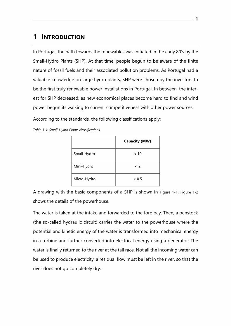
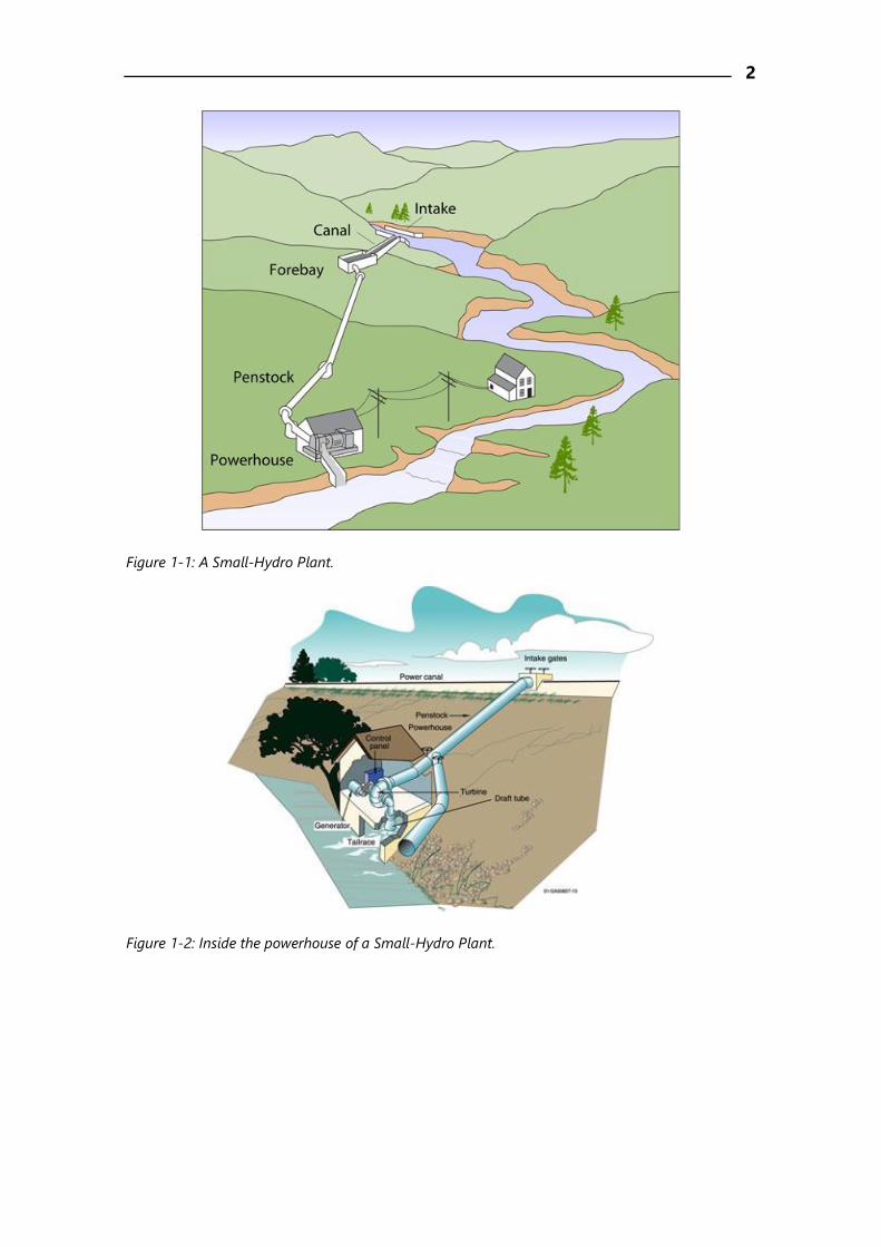
A drawing with the basic components of a SHP is shown in Figure 1-1. Figure 1-2

shows the details of the powerhouse.

The water is taken at the intake and forwarded to the fore bay. Then, a penstock

(the so-called hydraulic circuit) carries the water to the powerhouse where the

potential and kinetic energy of the water is transformed into mechanical energy

in a turbine and further converted into electrical energy using a generator. The

water is finally returned to the river at the tail race. Not all the incoming water can

be used to produce electricity, a residual flow must be left in the river, so that the

river does not go completely dry.

2

Figure 1-1: A Small-Hydro Plant.

Figure 1-2: Inside the powerhouse of a Small-Hydro Plant.

3

2 FLOW DURATION CURVE

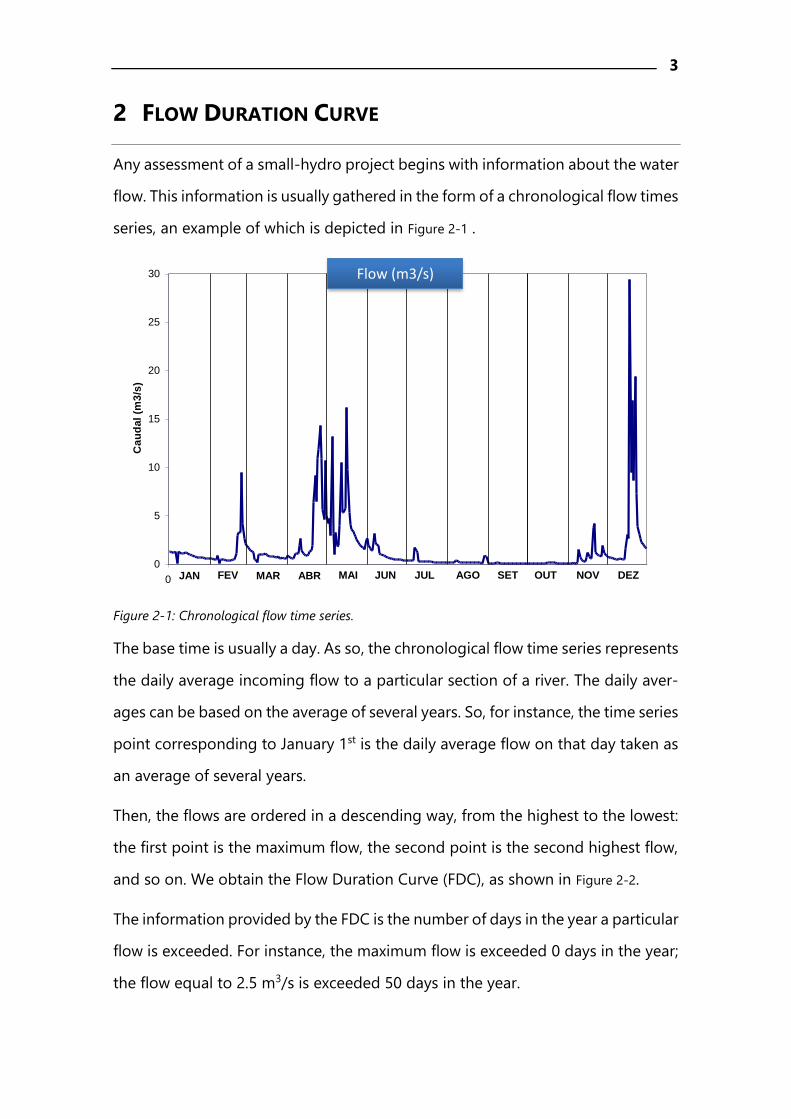
Any assessment of a small-hydro project begins with information about the water

flow. This information is usually gathered in the form of a chronological flow times

series, an example of which is depicted in Figure 2-1 .

Figure 2-1: Chronological flow time series.

The base time is usually a day. As so, the chronological flow time series represents

the daily average incoming flow to a particular section of a river. The daily aver-

ages can be based on the average of several years. So, for instance, the time series

point corresponding to January 1st is the daily average flow on that day taken as

an average of several years.

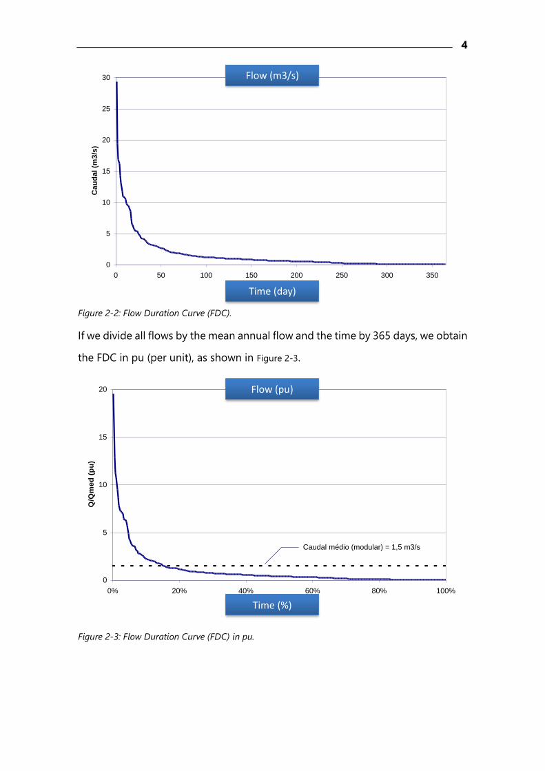
Then, the flows are ordered in a descending way, from the highest to the lowest:

the first point is the maximum flow, the second point is the second highest flow,

and so on. We obtain the Flow Duration Curve (FDC), as shown in Figure 2-2.

The information provided by the FDC is the number of days in the year a particular

flow is exceeded. For instance, the maximum flow is exceeded 0 days in the year;

the flow equal to 2.5 m3/s is exceeded 50 days in the year.

0

5

10

15

20

25

30

0

Ca

ud

al

(m3

/s)

JAN FEV MAR ABR MAI JUN JUL AGO SET OUT NOV DEZ

Flow (m3/s)

4

Figure 2-2: Flow Duration Curve (FDC).

If we divide all flows by the mean annual flow and the time by 365 days, we obtain

the FDC in pu (per unit), as shown in Figure 2-3.

Figure 2-3: Flow Duration Curve (FDC) in pu.

0

5

10

15

20

25

30

0 50 100 150 200 250 300 350

Tempo (dia)

Ca

ud

al

(m3

/s)

0

5

10

15

20

0% 20% 40% 60% 80% 100%

Tempo (%)

Q/Q

me

d (

pu

)

Caudal médio (modular) = 1,5 m3/s

Flow (m3/s)

Time (day)

Flow (pu)

Time (%)

5

3 TURBINE CHOICE

3.1 TURBINE TYPES

The detailed analysis of hydro turbines is outside the scope of this course. We

offer hereafter some basics on hydro turbines. Basically, there are two types of

hydro turbines: impulse turbines and reaction turbines.

In impulse turbines, the stator has nozzle jets and the rotor is a wheel with spoon-

shaped buckets, at atmospheric pressure. They are used for high heads and low

flows. Examples of impulse turbines are Pelton, Turgo and Banki-Mitchell hydro

turbines, Pelton being the most know type. In Figure 3-1, we show the rotor and

the nozzle jets of a Pelton turbine.

Figure 3-1: Rotor (left) and nozzle jets (right) of a Pelton turbine .

As far as reaction turbines are concerned, in the stator there is a distributor and

the rotor is composed of a runner, where the pressure is not constant and the

water is accelerated.

6

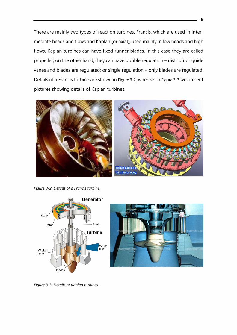
There are mainly two types of reaction turbines. Francis, which are used in inter-

mediate heads and flows and Kaplan (or axial), used mainly in low heads and high

flows. Kaplan turbines can have fixed runner blades, in this case they are called

propeller; on the other hand, they can have double regulation – distributor guide

vanes and blades are regulated; or single regulation – only blades are regulated.

Details of a Francis turbine are shown in Figure 3-2, whereas in Figure 3-3 we present

pictures showing details of Kaplan turbines.

Figure 3-2: Details of a Francis turbine.

Figure 3-3: Details of Kaplan turbines.

7

3.2 TURBINE EFFICIENCY

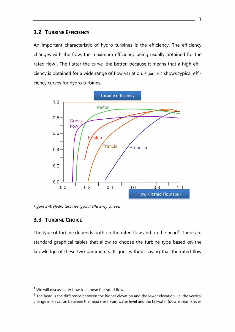
An important characteristic of hydro turbines is the efficiency. The efficiency

changes with the flow, the maximum efficiency being usually obtained for the

rated flow1. The flatter the curve, the better, because it means that a high effi-

ciency is obtained for a wide range of flow variation. Figure 3-4 shows typical effi-

ciency curves for hydro turbines.

Figure 3-4: Hydro turbines typical efficiency curves.

3.3 TURBINE CHOICE

The type of turbine depends both on the rated flow and on the head2. There are

standard graphical tables that allow to choose the turbine type based on the

knowledge of these two parameters. It goes without saying that the rated flow

1 We will discuss later how to choose the rated flow. 2 The head is the difference between the higher elevation and the lower elevation, i.e. the vertical

change in elevation between the head (reservoir) water level and the tailwater (downstream) level.

Turbine efficiency

Flow / Rated Flow (pu)

8

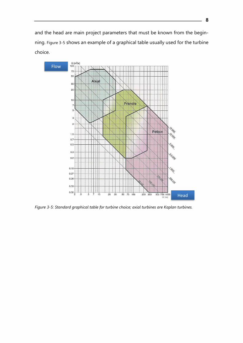
and the head are main project parameters that must be known from the begin-

ning. Figure 3-5 shows an example of a graphical table usually used for the turbine

choice.

Figure 3-5: Standard graphical table for turbine choice; axial turbines are Kaplan turbines.

Flow

Head

9

4 ELECTRICAL ENERGY YIELD – SIMPLIFIED MODEL

In this chapter, we are going through a simplified model to compute the electrical

energy yield of a small-hydro power plant. This model is used in early stages of

the project and provides an estimation of the electricity production that can be

expected.

The first step is to define the rated flow. In the past, the project engineer selected

the rated flow based on his own experience, his choice usually laying in a rated

flow that is exceeded in 15% to 40% of the time. Nowadays, powerful computa-

tion tools are available and the rated flow is chosen as the one that maximizes an

economic assessment index, the NPV, for instance. The process of selecting the

rated flow is therefore an iterative process.

The first approach for the rated flow is usually to take it as the mean annual flow.

Then, the electricity production is computed and a NPV is obtained. The process

is repeated for different values of the rated flow, the final decision being the rated

flow that maximizes the NPV. In what follows, it is assumed that the rated flow is

known.

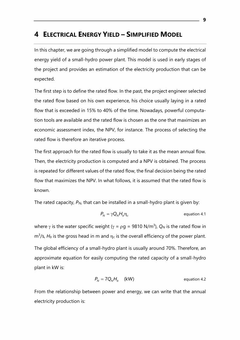
The rated capacity, PN, that can be installed in a small-hydro plant is given by:

N N b cP Q H equation 4.1

where is the water specific weight ( = g = 9810 N/m3), QN is the rated flow in

m3/s, Hb is the gross head in m and c is the overall efficiency of the power plant.

The global efficiency of a small-hydro plant is usually around 70%. Therefore, an

approximate equation for easily computing the rated capacity of a small-hydro

plant in kW is:

7 (kW)N N bP Q H equation 4.2

From the relationship between power and energy, we can write that the annual

electricity production is:

10

( ) 9810 ( ) ( ) ( )a uE P t dt Q t h t t dt equation 4.3

where we assume that all quantities in equation 4.1 can change in time. hu is the

useful head (gross head minus all the hydraulic losses) and is the combined

efficiency of the turbine, generator, transformer and auxiliary equipment.

4.1 ONE SINGLE TURBINE

To begin with, we shall address the case of a small-hydro plant equipped with a

single turbine.

We target a simplified model. So, we assume that both the head and the efficiency

are constant. The head is equal to the gross head and the overall efficiency is

around 70%.

We have to take a closer look at the flow, which is impossible to assume as con-

stant, because it is apparent from the FDC that it changes. The process to take

the flow variation into account will be described next.

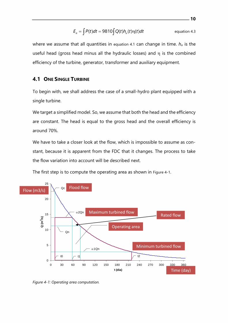
The first step is to compute the operating area as shown in Figure 4-1.

Figure 4-1: Operating area computation.

0

5

10

15

20

25

0 30 60 90 120 150 180 210 240 270 300 330 360

t (dia)

Q (

m3/s

)

Qc

Qn

2Qn

1Qn

Área de exploração

t0 t2t1

Flow (m3/s)

Time (day)

Operating area

Flood flow

Maximum turbined flow

Minimum turbined flow

Rated flow

11

The rated flow, which is assumed to be known is marked in the FDC. Only for the

purpose of this simplified model, two factors are defined for each type of hydro

turbine:

1

2

mT

N

MT

N

Q

Q

Q

Q

equation 4.4

where QMT is the maximum turbined flow, QmT is the minimum turbined flow and

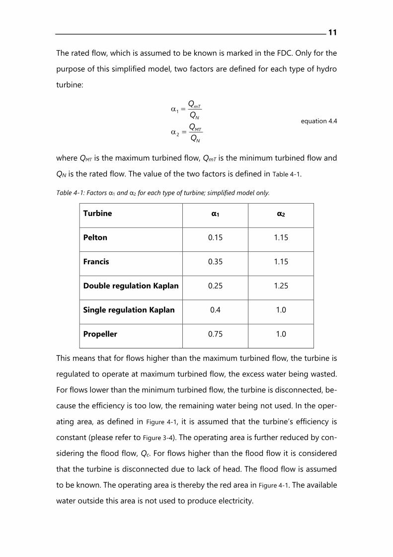
QN is the rated flow. The value of the two factors is defined in Table 4-1.

Table 4-1: Factors α1 and α2 for each type of turbine; simplified model only.

Turbine α1 α2

Pelton 0.15 1.15

Francis 0.35 1.15

Double regulation Kaplan 0.25 1.25

Single regulation Kaplan 0.4 1.0

Propeller 0.75 1.0

This means that for flows higher than the maximum turbined flow, the turbine is

regulated to operate at maximum turbined flow, the excess water being wasted.

For flows lower than the minimum turbined flow, the turbine is disconnected, be-

cause the efficiency is too low, the remaining water being not used. In the oper-

ating area, as defined in Figure 4-1, it is assumed that the turbine’s efficiency is

constant (please refer to Figure 3-4). The operating area is further reduced by con-

sidering the flood flow, Qc. For flows higher than the flood flow it is considered

that the turbine is disconnected due to lack of head. The flood flow is assumed

to be known. The operating area is thereby the red area in Figure 4-1. The available

water outside this area is not used to produce electricity.

12

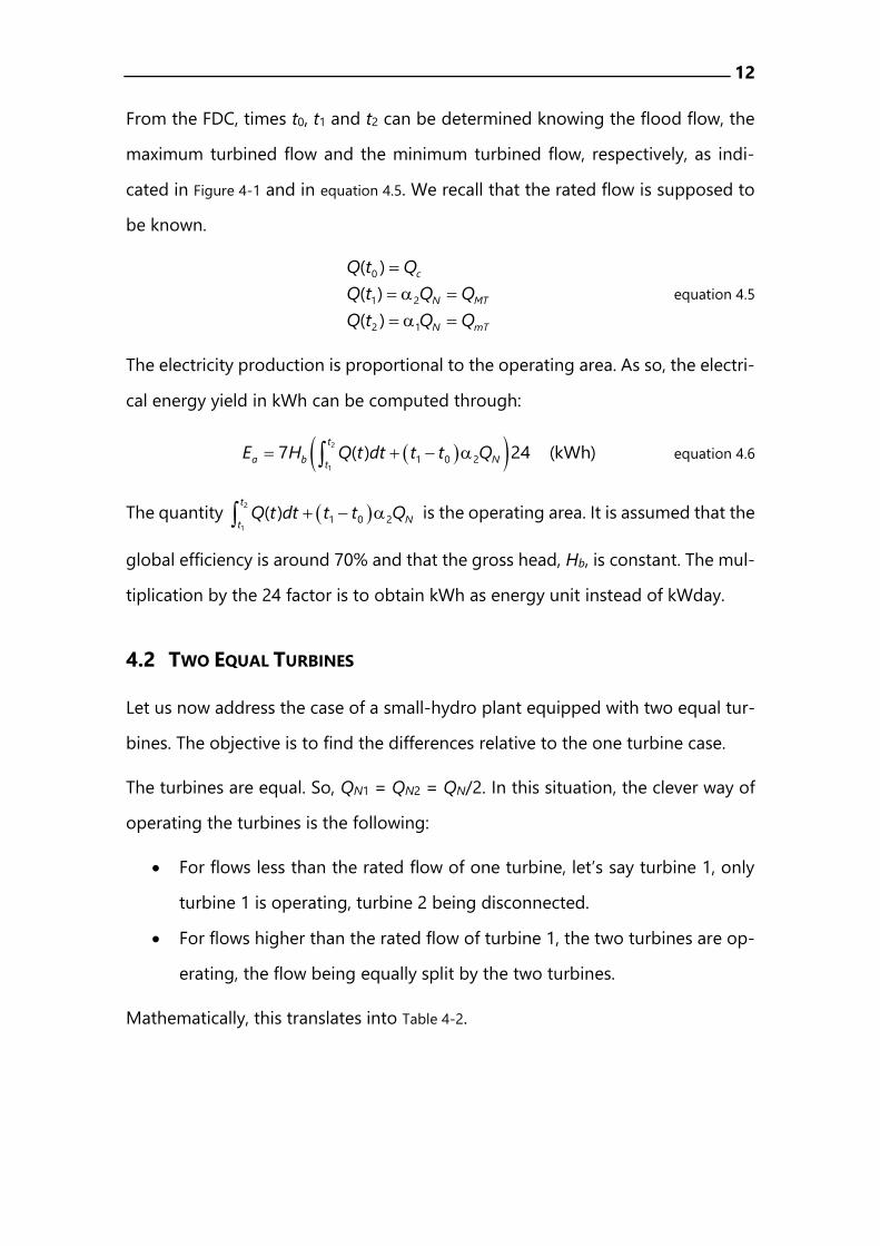
From the FDC, times t0, t1 and t2 can be determined knowing the flood flow, the

maximum turbined flow and the minimum turbined flow, respectively, as indi-

cated in Figure 4-1 and in equation 4.5. We recall that the rated flow is supposed to

be known.

0

1 2

2 1

( )

( )

( )

c

N MT

N mT

Q t Q

Q t Q Q

Q t Q Q

equation 4.5

The electricity production is proportional to the operating area. As so, the electri-

cal energy yield in kWh can be computed through:

2

11 0 27 ( ) 24 (kWh)

t

a b Nt

E H Q t dt t t Q equation 4.6

The quantity 2

11 0 2( )

t

Nt

Q t dt t t Q is the operating area. It is assumed that the

global efficiency is around 70% and that the gross head, Hb, is constant. The mul-

tiplication by the 24 factor is to obtain kWh as energy unit instead of kWday.

4.2 TWO EQUAL TURBINES

Let us now address the case of a small-hydro plant equipped with two equal tur-

bines. The objective is to find the differences relative to the one turbine case.

The turbines are equal. So, QN1 = QN2 = QN/2. In this situation, the clever way of

operating the turbines is the following:

For flows less than the rated flow of one turbine, let’s say turbine 1, only

turbine 1 is operating, turbine 2 being disconnected.

For flows higher than the rated flow of turbine 1, the two turbines are op-

erating, the flow being equally split by the two turbines.

Mathematically, this translates into Table 4-2.

13

Table 4-2: Two equal turbines operating mode.

Qj Turbine 1 Turbine 2

0 Qj < QN/2 Qj 0

QN/2 < Qj α2QN Qj/2 Qj/2

This is clever because it is better, from an efficiency point-of-view, to have one

turbine at full capacity than two turbines at half capacity.

The maximum turbined flow is unchanged relatively to the single turbine case,

because:

2

2 2

1

MT Ni N

i

Q Q Q

equation 4.7

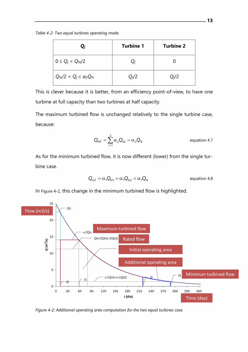
As for the minimum turbined flow, it is now different (lower) from the single tur-

bine case.

1 1 1 2 1mT N N NQ Q Q Q equation 4.8

In Figure 4-2, this change in the minimum turbined flow is highlighted.

Figure 4-2: Additional operating area computation for the two equal turbines case.

0

5

10

15

20

25

0 30 60 90 120 150 180 210 240 270 300 330 360

t (dia)

Q (

m3/s

)

Qc

Qn=2Qn1=2Qn2

2Qn

1Qn1=1Qn2

Área de exploração

t0

t2t1

t3

Área adicional 2

Flow (m3/s)

Time (day)

Additional operating area

Maximum turbined flow

Minimum turbined flow

Rated flow

Initial operating area

14

A new time t3 is now defined as:

3 1 1 1( )2

NN

QQ t Q equation 4.9

The total energy produced in the case the small hydro plant is equipped with two

equal turbines is:

3

11 0 27 ( ) 24 (kWh)

t

a b Nt

E H Q t dt t t Q equation 4.10

Comparing equation 4.6 and equation 4.10, it is apparent that, for the same installed

capacity, a small-hydro plant equipped with two turbines will produce always

more energy than if it is equipped with a single turbine. This is because, a smaller

turbine can pick-up lower flows. However, this does not mean that a two turbine

installation is better than a single turbine one. Indeed, for the same installed ca-

pacity, the cost of two equally sized turbines, with half the rated capacity each, is

higher than the cost of a full rated capacity single turbine. The same applies for

the O&M costs. The best solution is provided by the NPV computation, which

determines if the increased investment is compensated by increased production.

15

5 ELECTRICAL ENERGY YIELD – INTRODUCTION TO THE

DETAILED MODEL

In a design phase, more detailed models are needed to compute the electrical

energy yield of a small-hydro plant. One of these models is going to be presented

next.

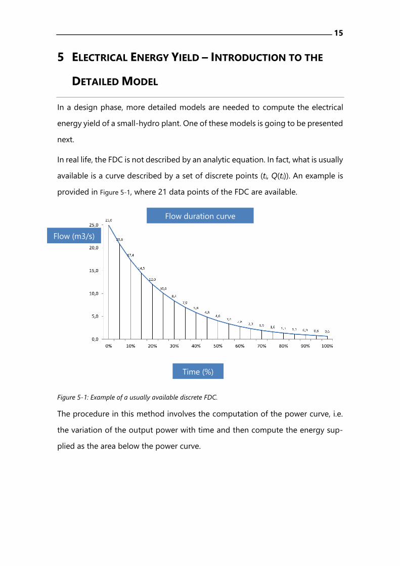
In real life, the FDC is not described by an analytic equation. In fact, what is usually

available is a curve described by a set of discrete points (ti, Q(ti)). An example is

provided in Figure 5-1, where 21 data points of the FDC are available.

Figure 5-1: Example of a usually available discrete FDC.

The procedure in this method involves the computation of the power curve, i.e.

the variation of the output power with time and then compute the energy sup-

plied as the area below the power curve.

Flow (m3/s)

Time (%)

Flow duration curve

16

5.1 COMPUTING THE OUTPUT POWER AS A FUNCTION OF THE FLOW

The general equation to compute the output electrical power as a function of the

incoming flow is:

_ _ _( ) ( ) ( ) ( ) (1 )i i u b hydr i u flood i t i u g transfo otherP Q Q H h Q h Q Q p equation 5.1

where:

P is the electrical power output in W.

Qi is the incoming flow at point i of the FDC in m3/s.

is the water specific weight 9810 N/m3.

Hb is the gross head in m.

hhydr are the hydraulic circuit losses for the used flow Qi_u in m.

Qi_u is the used flow in m, which is the flow that is forwarded to the turbine.

hflood are the flood losses for the incoming flow Qi in m.

t is the turbine efficiency for the used flow Qi_u.

g is the generator efficiency, which is assumed to be constant.

transfo is the transformer efficiency, which is assumed to be constant.

pother are other losses, e.g. in the auxiliary services of the power station,

which are assumed to be constant.

A residual flow must be left in the river, so that the riverbed is not dry. We, there-

fore, define the available flow, Q’i, as:

' max( ; 0)i i rQ Q Q equation 5.2

where Qr is the residual flow. The residual flow must be known, normally it is

about 3%–5% of the rated flow.

In this model, it is assumed that the maximum turbined flow is equal to the rated

flow. We recall that no α1 and α2 apply in the detailed model. Thus, the used flow,

i.e. the flow that is forwarded to the turbine, is:

_ min( ' ; )i u i NQ Q Q equation 5.3

17

The hydraulic circuit losses are losses inside the pipes (penstock) that carry the

water from the higher elevation to the powerhouse. The hydraulic circuit head

losses are proportional to the square of the flow, in the same way the Joule losses

are proportional to the square of the current, in electrical circuits. Accordingly, we

can write:

2

_max i u

hydr b hydr

N

Qh H p

Q

equation 5.4

where max

hydrp is the maximum value of the hydraulic circuit losses as a percentage

of the gross head, Hb. Its value must be known, a common value being about 3%–

5%. Of course, the hydraulic circuit losses depend upon the used flow, as this is

the turbined flow, the one that travels inside the penstock. These losses are max-

imum for the rated flow, which is the maximum turbined flow.

The flood flow losses are not related to the used flow, but instead to the incoming

flow. In fact, a flood flow causes a reduction in the available head, this reduction

being accounted for in this parameter. The flood losses are maximum for the

maximum incoming flow and are null for the rated flow. It makes no sense to

compute the flood losses for flows lower than the rated flow, because these flows

do not cause flood. Hence, the flood flow losses can be written as:

2

max

max

i Nflood flood i N

N

Q Qh h Q Q

Q Q

equation 5.5

where max

floodh is the maximum value of the flood losses in m, which must be known

or estimated somehow. Qmax is the maximum incoming flow (the maximum of the

FDC).

The efficiency of the turbine is specific of each turbine. Analysing several efficiency

curves for the different types of turbines, as the ones showed in Figure 3-4, the

following general-purpose model for the efficiency of any turbine was built:

18

_1 1 i u

t

N

Q

Q

equation 5.6

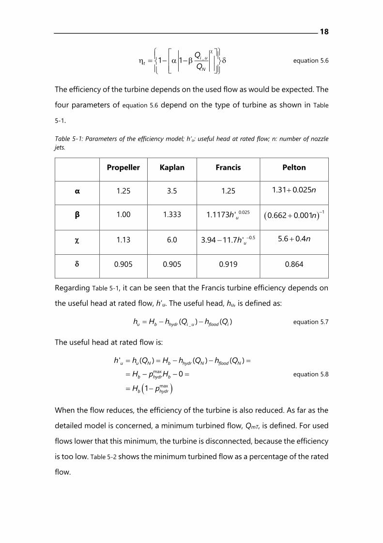
The efficiency of the turbine depends on the used flow as would be expected. The

four parameters of equation 5.6 depend on the type of turbine as shown in Table

5-1.

Table 5-1: Parameters of the efficiency model; h’u: useful head at rated flow; n: number of nozzle

jets.

Propeller Kaplan Francis Pelton

α 1.25 3.5 1.25 1.31 0.025n

β 1.00 1.333 0.0251.1173 'uh 1

0.662 0.001n

1.13 6.0 0.53.94 11.7 'uh 5.6 0.4n

0.905 0.905 0.919 0.864

Regarding Table 5-1, it can be seen that the Francis turbine efficiency depends on

the useful head at rated flow, h’u. The useful head, hu, is defined as:

_( ) ( )u b hydr i u flood ih H h Q h Q equation 5.7

The useful head at rated flow is:

max

max

' ( ) ( ) ( )

0

1

u u N b hydr N flood N

b hydr b

b hydr

h h Q H h Q h Q

H p H

H p

equation 5.8

When the flow reduces, the efficiency of the turbine is also reduced. As far as the

detailed model is concerned, a minimum turbined flow, QmT, is defined. For used

flows lower that this minimum, the turbine is disconnected, because the efficiency

is too low. Table 5-2 shows the minimum turbined flow as a percentage of the rated

flow.

19

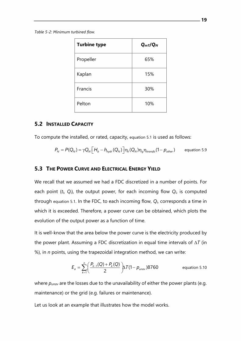
Table 5-2: Minimum turbined flow.

Turbine type QmT/QN

Propeller 65%

Kaplan 15%

Francis 30%

Pelton 10%

5.2 INSTALLED CAPACITY

To compute the installed, or rated, capacity, equation 5.1 is used as follows:

( ) ( ) ( ) (1 )N N N b hydr N t N g transfo otherP P Q Q H h Q Q p equation 5.9

5.3 THE POWER CURVE AND ELECTRICAL ENERGY YIELD

We recall that we assumed we had a FDC discretized in a number of points. For

each point (ti, Qi), the output power, for each incoming flow Qi, is computed

through equation 5.1. In the FDC, to each incoming flow, Qi, corresponds a time in

which it is exceeded. Therefore, a power curve can be obtained, which plots the

evolution of the output power as a function of time.

It is well-know that the area below the power curve is the electricity produced by

the power plant. Assuming a FDC discretization in equal time intervals of T (in

%), in n points, using the trapezoidal integration method, we can write:

1

1

( ) ( )(1 )8760

2

nk k

a unav

k

P Q P QE T p

equation 5.10

where punav are the losses due to the unavailability of either the power plants (e.g.

maintenance) or the grid (e.g. failures or maintenance).

Let us look at an example that illustrates how the model works.

20

Example 5—1

Consider a SHP with a gross head of 6.35 m where the FDC is described by

( ) 25exp 100Q t t (t in days and Q in m3/s). The maximum hydraulic circuit

head losses are 4% and the maximum flood losses are 6.1 m. The efficiencies of the

generator and transformer are 95% and 99%, respectively, and other losses can be

fixed in 2%. The unavailability losses are estimated in 4%. The SHP is equipped with

a double regulation Kaplan turbine. The rated flow is 11.25 m3/s and the residual

ecologic flow is 1 m3/s. Compute the annual electricity yield of the SHP.

Solution:

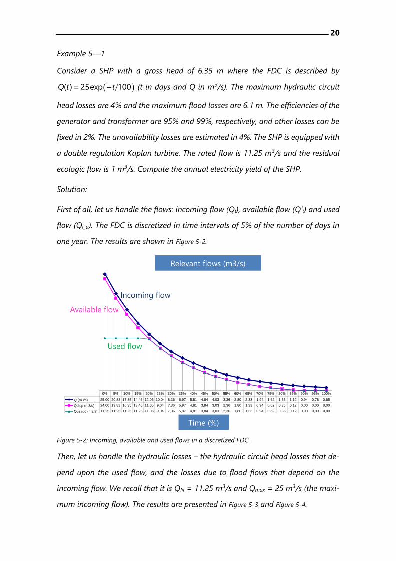
First of all, let us handle the flows: incoming flow (Qi), available flow (Q’i) and used

flow (Qi_u). The FDC is discretized in time intervals of 5% of the number of days in

one year. The results are shown in Figure 5-2.

Figure 5-2: Incoming, available and used flows in a discretized FDC.

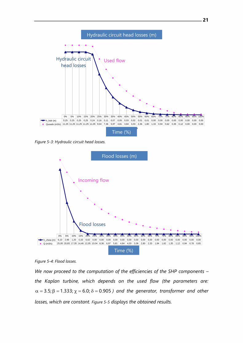
Then, let us handle the hydraulic losses – the hydraulic circuit head losses that de-

pend upon the used flow, and the losses due to flood flows that depend on the

incoming flow. We recall that it is QN = 11.25 m3/s and Qmax = 25 m3/s (the maxi-

mum incoming flow). The results are presented in Figure 5-3 and Figure 5-4.

Curvas de duração de caudais (m3/s)

Tempo

Q (m3/s) 25,00 20,83 17,35 14,46 12,05 10,04 8,36 6,97 5,81 4,84 4,03 3,36 2,80 2,33 1,94 1,62 1,35 1,12 0,94 0,78 0,65

Qdisp (m3/s) 24,00 19,83 16,35 13,46 11,05 9,04 7,36 5,97 4,81 3,84 3,03 2,36 1,80 1,33 0,94 0,62 0,35 0,12 0,00 0,00 0,00

Qusado (m3/s) 11,25 11,25 11,25 11,25 11,05 9,04 7,36 5,97 4,81 3,84 3,03 2,36 1,80 1,33 0,94 0,62 0,35 0,12 0,00 0,00 0,00

0% 5% 10% 15% 20% 25% 30% 35% 40% 45% 50% 55% 60% 65% 70% 75% 80% 85% 90% 95% 100%

Time (%)

Relevant flows (m3/s)

Incoming flow

Available flow

Used flow

21

Figure 5-3: Hydraulic circuit head losses.

Figure 5-4: Flood losses.

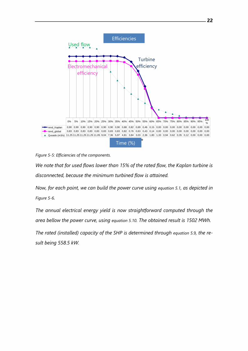
We now proceed to the computation of the efficiencies of the SHP components –

the Kaplan turbine, which depends on the used flow (the parameters are:

3.5; 1.333; 6.0; 0.905 ) and the generator, transformer and other

losses, which are constant. Figure 5-5 displays the obtained results.

Altura de perdas no circuito hidráulico (m)

Tempo

h_hidr (m) 0,25 0,25 0,25 0,25 0,24 0,16 0,11 0,07 0,05 0,03 0,02 0,01 0,01 0,00 0,00 0,00 0,00 0,00 0,00 0,00 0,00

Qusado (m3/s) 11,25 11,25 11,25 11,25 11,05 9,04 7,36 5,97 4,81 3,84 3,03 2,36 1,80 1,33 0,94 0,62 0,35 0,12 0,00 0,00 0,00

0% 5% 10% 15% 20% 25% 30% 35% 40% 45% 50% 55% 60% 65% 70% 75% 80% 85% 90% 95% 100%

Altura de perdas dos caudais de cheia (m)

Tempo

h_cheia (m) 6,10 2,96 1,20 0,33 0,02 0,00 0,00 0,00 0,00 0,00 0,00 0,00 0,00 0,00 0,00 0,00 0,00 0,00 0,00 0,00 0,00

Q (m3/s) 25,00 20,83 17,35 14,46 12,05 10,04 8,36 6,97 5,81 4,84 4,03 3,36 2,80 2,33 1,94 1,62 1,35 1,12 0,94 0,78 0,65

0% 5% 10% 15% 20% 25% 30% 35% 40% 45% 50% 55% 60% 65% 70% 75% 80% 85% 90% 95% 100%

Time (%)

Hydraulic circuit head losses (m)

Used flow Hydraulic circuit

head losses

Time (%)

Flood losses (m)

Incoming flow

Flood losses

22

Figure 5-5: Efficiencies of the components.

We note that for used flows lower than 15% of the rated flow, the Kaplan turbine is

disconnected, because the minimum turbined flow is attained.

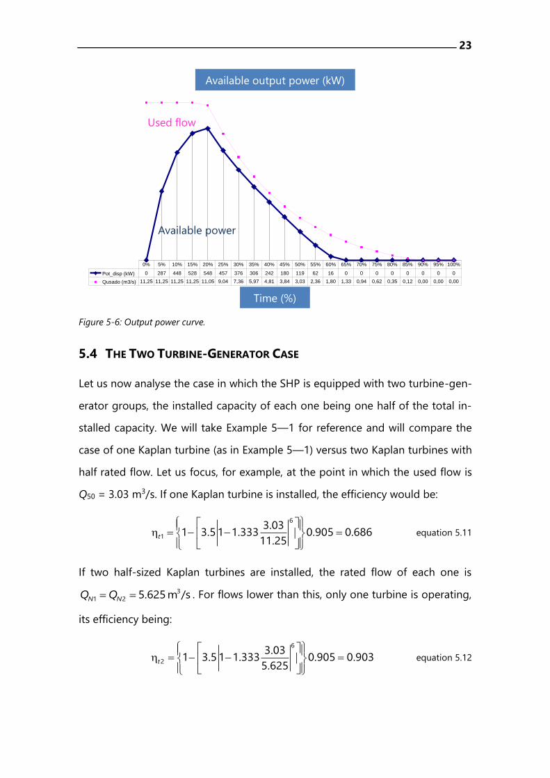
Now, for each point, we can build the power curve using equation 5.1, as depicted in

Figure 5-6.

The annual electrical energy yield is now straightforward computed through the

area bellow the power curve, using equation 5.10. The obtained result is 1502 MWh.

The rated (installed) capacity of the SHP is determined through equation 5.9, the re-

sult being 558.5 kW.

Rendimentos

Tempo

rend_Kaplan 0,90 0,90 0,90 0,90 0,90 0,90 0,90 0,90 0,88 0,82 0,69 0,46 0,15 0,00 0,00 0,00 0,00 0,00 0,00 0,00 0,00

rend_global 0,83 0,83 0,83 0,83 0,83 0,83 0,83 0,83 0,82 0,76 0,63 0,43 0,14 0,00 0,00 0,00 0,00 0,00 0,00 0,00 0,00

Qusado (m3/s) 11,25 11,25 11,25 11,25 11,05 9,04 7,36 5,97 4,81 3,84 3,03 2,36 1,80 1,33 0,94 0,62 0,35 0,12 0,00 0,00 0,00

0% 5% 10% 15% 20% 25% 30% 35% 40% 45% 50% 55% 60% 65% 70% 75% 80% 85% 90% 95%100

%

Turbine

efficiency

Time (%)

Efficiencies

Used flow

Electromechanical

efficiency

23

Figure 5-6: Output power curve.

5.4 THE TWO TURBINE-GENERATOR CASE

Let us now analyse the case in which the SHP is equipped with two turbine-gen-

erator groups, the installed capacity of each one being one half of the total in-

stalled capacity. We will take Example 5—1 for reference and will compare the

case of one Kaplan turbine (as in Example 5—1) versus two Kaplan turbines with

half rated flow. Let us focus, for example, at the point in which the used flow is

Q50 = 3.03 m3/s. If one Kaplan turbine is installed, the efficiency would be:

6

1

3.031 3.5 1 1.333 0.905 0.686

11.25t

equation 5.11

If two half-sized Kaplan turbines are installed, the rated flow of each one is

3

1 2 5.625 m /sN NQ Q . For flows lower than this, only one turbine is operating,

its efficiency being:

6

2

3.031 3.5 1 1.333 0.905 0.903

5.625t

equation 5.12

Potência disponível (kW)

Tempo

Pot_disp (kW) 0 287 448 528 548 457 376 306 242 180 119 62 16 0 0 0 0 0 0 0 0

Qusado (m3/s) 11,25 11,25 11,25 11,25 11,05 9,04 7,36 5,97 4,81 3,84 3,03 2,36 1,80 1,33 0,94 0,62 0,35 0,12 0,00 0,00 0,00

0% 5% 10% 15% 20% 25% 30% 35% 40% 45% 50% 55% 60% 65% 70% 75% 80% 85% 90% 95% 100%

Time (%)

Available output power (kW)

Used flow

Available power

24

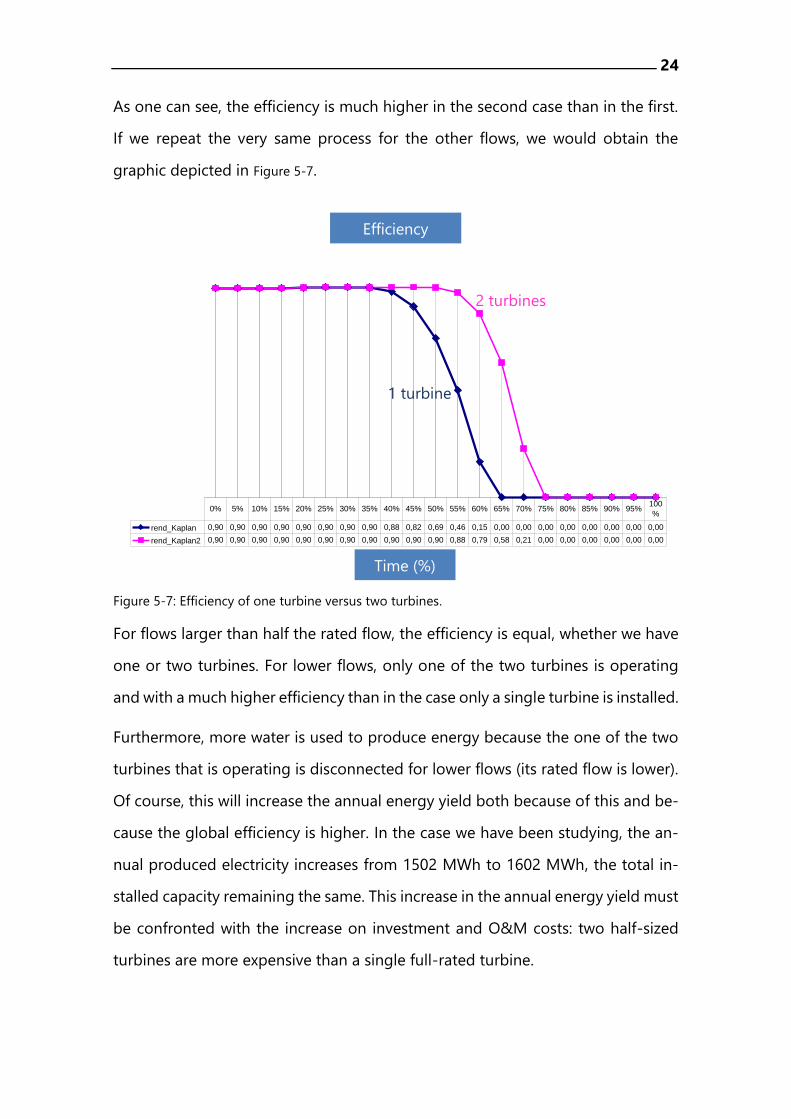
As one can see, the efficiency is much higher in the second case than in the first.

If we repeat the very same process for the other flows, we would obtain the

graphic depicted in Figure 5-7.

Figure 5-7: Efficiency of one turbine versus two turbines.

For flows larger than half the rated flow, the efficiency is equal, whether we have

one or two turbines. For lower flows, only one of the two turbines is operating

and with a much higher efficiency than in the case only a single turbine is installed.

Furthermore, more water is used to produce energy because the one of the two

turbines that is operating is disconnected for lower flows (its rated flow is lower).

Of course, this will increase the annual energy yield both because of this and be-

cause the global efficiency is higher. In the case we have been studying, the an-

nual produced electricity increases from 1502 MWh to 1602 MWh, the total in-

stalled capacity remaining the same. This increase in the annual energy yield must

be confronted with the increase on investment and O&M costs: two half-sized

turbines are more expensive than a single full-rated turbine.

Rendimentos

Tempo

rend_Kaplan 0,90 0,90 0,90 0,90 0,90 0,90 0,90 0,90 0,88 0,82 0,69 0,46 0,15 0,00 0,00 0,00 0,00 0,00 0,00 0,00 0,00

rend_Kaplan2 0,90 0,90 0,90 0,90 0,90 0,90 0,90 0,90 0,90 0,90 0,90 0,88 0,79 0,58 0,21 0,00 0,00 0,00 0,00 0,00 0,00

0% 5% 10% 15% 20% 25% 30% 35% 40% 45% 50% 55% 60% 65% 70% 75% 80% 85% 90% 95%100

%

Time (%)

Efficiency

2 turbines

1 turbine