Embed Size (px)
Citation preview
Rendering High Detail Models from Displacement Maps
Martin Volovar∗
Supervised by: Peter Drahos†
Institute of Applied InformaticsFaculty of Informatics and Information Technologies
Slovak Technical UniversityBratislava / Slovakia
Abstract
In this paper, we present a method to generate a high res-olution mesh from low poly mesh directly on GPU to re-duce bandwidth overhead between GPU and CPU. We useknown methods such as subdivision surface, displacementmapping and adaptive tessellation to generate more geom-etry in certain parts where it is necessary. This methodis suitable for animation because small numbers of controlpoints are modified. The main aim of this work is effectiverender a high quality mesh in the real time.
Keywords: Vector displacement map, Adaptive tessella-tion, Feature adaptive subdivision
1 Introduction
Since the first GPU has been released, GPU performancehas been highly increased. Modern high-end GPUs canrender around 6 billion triangles per second [11]. Mem-ory bandwidth and an I/O latency has been improved too,but not as much as GPU render speed. What was notlimiting factor before, is now a performance bottleneck.Transferring data between CPU and GPU is not a prob-lem if a model geometry is static. In case of a model ani-mation, modifying complex objects on CPU and updatingGPU buffers can be impossible for every frame [9]. Mo-tivation is to transfer only small parts of data and calcu-late model on GPU instead of transferring whole updatedmodel. These parts could be changed position of controlvertices or a changed sub-image of a displacement map.
Further motivation is to take advantage of adding de-tail dynamically in certain parts of model. This allowsto change a complexity of a model according to its flat-ness and a screen space area. There is a similar methodnamed LOD (Level of detail), which uses pre-generatedmodels in different resolutions, but that method requiresmore memory and there is a problem in a continuity whenthe resolution is switched.
∗[email protected]†peter [email protected]
2 Background
This section describes methods to generate high detailmesh from control mesh.
2.1 Subdivision surfaces
Smooth surfaces often occur in the nature. Traditionalmethod, polygon surface, requires many polygons to ap-proximate a smoothness [4]. Geometric modelling of com-plex models is problematic. In the past, memory for stor-ing complex models was expensive. Using subdivisionsurfaces it is possible save memory storage.
Subdivision surfaces are a curved-surface representa-tion defined by a control mesh [2]. Subdivision surfacesmooths initial model using recursive subdivision algo-rithm [3]. Subdivision level depends on how many subdi-vision steps are required. Subdivision step has two stages:mesh refinement and vertex placement. Mesh refinementsubdivide every face and edge. Vertex placement set vertexposition according to subdivision rule. Position is calcu-lated by linear interpolation of neighbour vertices.
Hypothetical surface created after an infinite number ofsubdivision steps is called limit surface [2]. The limit sur-face has often C2 continuity everywhere, except at extraor-dinary vertices [10]. The most well-known subdivision al-gorithm for quad meshes is Catmull-Clark.
Adaptive subdivision allows to use different subdivisionlevel on certain parts of mesh. Adaptive subdivision usesflatness test to avoid subdividing flat parts of model [2].
In feature adaptive subdivision method, the limit sub-division surface is described by a collection of bi-cubicB-spline patches [8]. This is advantage because patchescan be rendered directly using hardware tessellation. In-stead of uniform subdivision, where geometry complexitygrows exponentially, using feature adaptive subdivision,complexity is close to linear [6].
2.2 Tessellation
Tessellation is the process of breaking patch into manysmaller primitives [11]. Patch is defined as set of controlpoints. Patch type can be line, triangle, quad, B-Spline,
Proceedings of CESCG 2016: The 20th Central European Seminar on Computer Graphics (non-peer-reviewed)
Bezier, etc. Tessellation factor controls fineness of patch.Adjacent edges should have the same tessellation factorbecause T-vertices could create a crack. Tessellation canconvert quads to triangles, but common usage is to add ge-ometric detail. Tessellation is now hardware accelerated.
2.3 Displacement mapping
Displacement mapping is using with tessellation to addhigh frequency detail with low memory I/O [7]. Instead ofcreating a smooth surface with subdivision surface, usingdisplacement mapping it is possible make a rough surface.
A displacement map is a special type of texture wherethe stored values refer to a displacement of a vector. Acommonly used type of displacement maps is the scalardisplacement map, where each value corresponds to a dis-placement along the normal vector of a vertex. Scalar dis-placement map is easy to compute since normal vectorsare cached. With vector displacement map it is possibledisplace vertex to any direction. Vector displacement maprequires more memory than scalar because it uses all tan-gent vectors - t, b, n.
3 Our Contribution
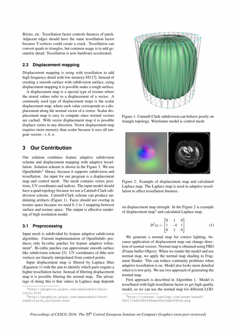
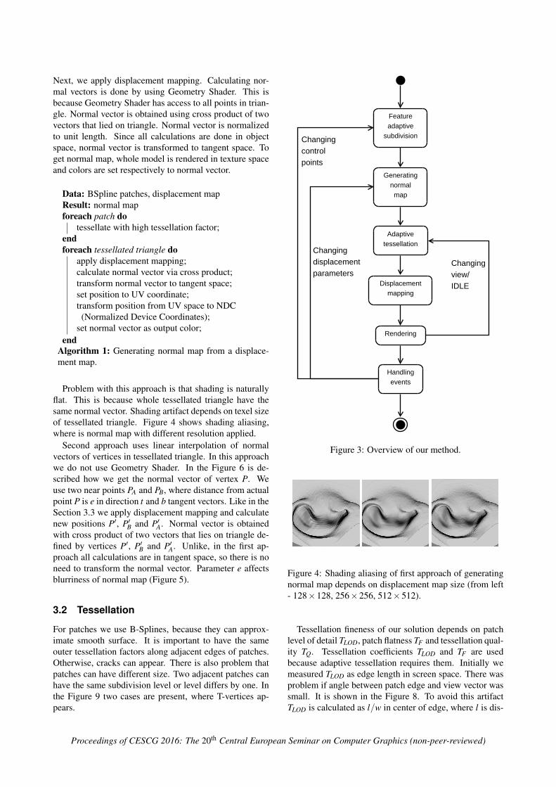
Our solution combines feature adaptive subdivisionscheme and displacement mapping with adaptive tessel-lation. Solution scheme is shown in the Figure 3. We useOpenSubdiv1 library, because it supports subdivision andtessellation. An input for our program is a displacementmap and control mesh. The mesh contains vertex posi-tions, UV coordinates and indices. The input model shouldhave a quad topology because we use a Catmull-Clark sub-division scheme. Catmull-Clark scheme can produce un-dulating artifacts (Figure 1). Faces should not overlap intexture space because we need 0..1 to 1 mapping betweensurface and texture space. The output is effective render-ing of high resolution model.
3.1 Preprocessing
Input mesh is subdivided by feature adaptive subdivisionalgorithm. Current implementation of OpenSubdiv pro-duces only bi-cubic patches for feature adaptive refine-ment2. Bi-cubic patches can approximate smooth surfacelike subdivision scheme [5]. UV coordinates of thhe newvertices are linearly interpolated from control points.
Input displacement map is filtered by Laplace filter(Equation 1) with the aim to identify which parts require ahigher tessellation factor. Instead of filtering displacementmap it is possible filtering the normal map. The advan-tage of doing this is that values in Laplace map depends
1http://graphics.pixar.com/opensubdiv/docs/intro.html
2http://graphics.pixar.com/opensubdiv/docs/subdivision_surfaces.html
Figure 1: Catmull-Clark subdivision can behave poorly ontriangle topology. Wireframe model is control mesh.
Figure 2: Example of displacement map and calculatedLaplace map. The Laplace map is used in adaptive tessel-lation to affect tessellation fineness.
on displacement map strength. In the Figure 2 is exampleof displacement map3 and calculated Laplace map.
D2xy =
0 1 01 −4 10 1 0
(1)
We generate a normal map for correct lighting, be-cause application of displacement map can change direc-tion of normal vectors. Normal map is obtained using FBO(Frame buffer Object). When we render the model and usenormal map, we apply the normal map shading in Frag-ment Shader. This can reduce continuity problems whenadaptive tessellation is on. Model also looks more detailedwhen it is low poly. We use two approach of generating thenormal map.
First approach is described in Algorithm 1. Model istessellated with high tessellation factor to get high qualitymodel, so we can use the normal map for different LOD.
3http://content.luxology.com/asset/exref/fd5171e820982995daaf5e15db00955d.png
Proceedings of CESCG 2016: The 20th Central European Seminar on Computer Graphics (non-peer-reviewed)
Next, we apply displacement mapping. Calculating nor-mal vectors is done by using Geometry Shader. This isbecause Geometry Shader has access to all points in trian-gle. Normal vector is obtained using cross product of twovectors that lied on triangle. Normal vector is normalizedto unit length. Since all calculations are done in objectspace, normal vector is transformed to tangent space. Toget normal map, whole model is rendered in texture spaceand colors are set respectively to normal vector.
Data: BSpline patches, displacement mapResult: normal mapforeach patch do
tessellate with high tessellation factor;endforeach tessellated triangle do
apply displacement mapping;calculate normal vector via cross product;transform normal vector to tangent space;set position to UV coordinate;transform position from UV space to NDC
(Normalized Device Coordinates);set normal vector as output color;
endAlgorithm 1: Generating normal map from a displace-ment map.
Problem with this approach is that shading is naturallyflat. This is because whole tessellated triangle have thesame normal vector. Shading artifact depends on texel sizeof tessellated triangle. Figure 4 shows shading aliasing,where is normal map with different resolution applied.
Second approach uses linear interpolation of normalvectors of vertices in tessellated triangle. In this approachwe do not use Geometry Shader. In the Figure 6 is de-scribed how we get the normal vector of vertex P. Weuse two near points PA and PB, where distance from actualpoint P is e in direction t and b tangent vectors. Like in theSection 3.3 we apply displacement mapping and calculatenew positions P′, P′B and P′A. Normal vector is obtainedwith cross product of two vectors that lies on triangle de-fined by vertices P′, P′B and P′A. Unlike, in the first ap-proach all calculations are in tangent space, so there is noneed to transform the normal vector. Parameter e affectsblurriness of normal map (Figure 5).
3.2 Tessellation
For patches we use B-Splines, because they can approx-imate smooth surface. It is important to have the sameouter tessellation factors along adjacent edges of patches.Otherwise, cracks can appear. There is also problem thatpatches can have different size. Two adjacent patches canhave the same subdivision level or level differs by one. Inthe Figure 9 two cases are present, where T-vertices ap-pears.
Featureadaptive
subdivision
Generatingnormalmap
Adaptivetessellation
Displacementmapping
Rendering
Handlingevents
Changingcontrolpoints
Changingdisplacementparameters
Changingview/IDLE
Figure 3: Overview of our method.
Figure 4: Shading aliasing of first approach of generatingnormal map depends on displacement map size (from left- 128×128, 256×256, 512×512).
Tessellation fineness of our solution depends on patchlevel of detail TLOD, patch flatness TF and tessellation qual-ity TQ. Tessellation coefficients TLOD and TF are usedbecause adaptive tessellation requires them. Initially wemeasured TLOD as edge length in screen space. There wasproblem if angle between patch edge and view vector wassmall. It is shown in the Figure 8. To avoid this artifactTLOD is calculated as l/w in center of edge, where l is dis-
Proceedings of CESCG 2016: The 20th Central European Seminar on Computer Graphics (non-peer-reviewed)
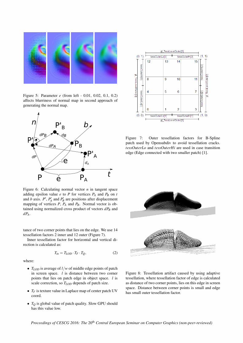
Figure 5: Parameter e (from left - 0.01, 0.02, 0.1, 0.2)affects blurriness of normal map in second approach ofgenerating the normal map.
P PA
PB
e
e
P'
t
b
P'A
P'BdPB
dPA
n
dB
dP
dA
Figure 6: Calculating normal vector n in tangent spaceadding epsilon value e to P for vertices PA and PB on tand b axis. P′, P′A and P′B are positions after displacementmapping of vertices P, PA and PB. Normal vector is ob-tained using normalized cross product of vectors dPB anddPA.
tance of two corner points that lies on the edge. We use 14tessellation factors 2 inner and 12 outer (Figure 7).
Inner tessellation factor for horizontal and vertical di-rection is calculated as:
Tin = TLOD ·TF ·TQ, (2)
where:
• TLOD is average of l/w of middle edge points of patchin screen space. l is distance between two cornerpoints that lies on patch edge in object space. l isscale correction, so TLOD depends of patch size.
• TF is texture value in Laplace map of center patch UVcoord.
• TQ is global value of patch quality. Slow GPU shouldhas this value low.
Figure 7: Outer tessellation factors for B-Splinepatch used by Opensubdiv to avoid tessellation cracks.tessOuterLo and tessOuterHi are used in case transitionedge (Edge connected with two smaller patch) [1].
Figure 8: Tessellation artifact caused by using adaptivetessellation, where tessellation factor of edge is calculatedas distance of two corner points, lies on this edge in screenspace. Distance between corner points is small and edgehas small outer tessellation factor.
Proceedings of CESCG 2016: The 20th Central European Seminar on Computer Graphics (non-peer-reviewed)

a) b)
Figure 9: T-vertices occur in edge where patch has a) samesubdivision level, but different outer tessellation factor onadjacent edge b) subdivision level that differs by one andtessOuterLo, tessOuterHi tessellation factors are not thesame as tessOuter of adjacent edge of smaller patch.
Tin is rounded to nearest integer value and clamped, sominimal value can be 1. This is because inner tessellationwith level less than 1 is undefined.
The easiest solution to avoid T-vertices is to set globalouter tessellation factor to a constant value and in case oftransition edge to double it. Problem with this solutionis that inner tessellation factors change over surface andouter tessellation factor does not have to suit well. Our ad-vanced method is based on simple idea that adjacent vertexhas the same UV coordinate. We use the same Equation 2like on inner tessellation factor, but coefficients TLOD andTF are calculated differently. For neighbour patches thatuses same subdivision level, TLOD is l/w of middle edgepoint in screen space. Else TLOD is calculated as l/w ofcenter in edge for Lo and Hi segments. If adjacent patchhave the same subdivision level then TF uses UV coordi-nate of middle point edge. In other case UV coordinate ischosen with weight 1/4 and 3/4 of corner UV coordinatesbecause it is center of edge in smaller patch.
3.3 Displacement mapping
We use a vector displacement map. Tangent vectors - t,b, n are calculated from barycentric patch coordinates andpatch parameters. Calculating a new position P′ of a vertexin an object space is in the Equation 3.
P′ =
PxPyPz
+ s ·
tx bx nxty by nytz bz nz
dr−odg−odb−o
, (3)
where:
• P′ is new position in object space after the displace-ment mapping.
• P is an old position in object space before the dis-placement mapping.
• t, b, n are unit tangent vectors defined in object space.
• s is a strength of displacement.
• d is a vector displacement value in displacement map.
Figure 10: Morphing animation using linear interpolationof two displacement map.
Figure 11: Animation, where control vertex is changing.
• o is a texture value, where displacement is zero. Forunsigned displacement map it should be zero and forsigned displacement map it should be set to 0.5.
4 Results
We can animate model changing displacement parametersor changing control points position. Our solutions canwith a small amount of control vertices change shape ofmodel (Figure 11). It is also possible to create morphinganimation with linear interpolation of two displacementmaps (Figure 10). Our solution uses adaptive tessellation,so generated geometry is view dependent (Figure 12). Inour tests we use Nvidia GT 740M GPU and i7-4702MQCPU.
Generating subdivision surface from control mesh isfast (Table 2) because we use feature adaptive subdivisionrather than uniform subdivision. Feature adaptive subdivi-sion is usually faster than uniform because feature adap-tive subdivision uses fewer patches than uniform subdivi-sion uses quads (Table 1). This is because bi-cubic patchescan better approximate limit surface. However, quad usesonly 4 vertices instead of 16 in case of B-Splines. Modelcomplexity of feature adaptive subdivision grows linearlyinstead of exponentially. CPU time is measured via highresolution timer4 in beginning and ending of generatingfunction. OpenGL functions can be asynchronous, soGPU time is measured using GL TIME ELAPSED query.
4https://msdn.microsoft.com/en-us/library/windows/desktop/dn553408
Proceedings of CESCG 2016: The 20th Central European Seminar on Computer Graphics (non-peer-reviewed)
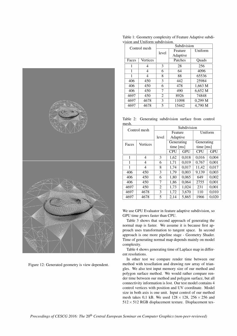
Figure 12: Generated geometry is view dependent.
Table 1: Geometry complexity of Feature Adaptive subdi-vision and Uniform subdivision.
Control mesh Subdivision
level FeatureAdaptive
Uniform
Faces Vertices Patches Quads1 4 3 28 2561 4 6 64 40961 4 8 88 65536
406 450 3 442 25984406 450 6 478 1,663 M406 450 7 490 6,652 M4697 450 2 8926 748484697 4678 3 11098 0,299 M4697 4678 5 15442 4,790 M
Table 2: Generating subdivision surface from controlmesh.
Control mesh Subdivision
levelFeature
AdaptiveUniform
Faces Vertices Generatingtime [ms]
Generatingtime [ms]
CPU GPU CPU GPU1 4 3 1,62 0,018 0,016 0,0041 4 6 1,71 0,019 0,767 0,0011 4 8 1,74 0,017 11,42 0,017
406 450 3 1,79 0,003 9,139 0,003406 450 6 1,80 0,065 649 0,002406 450 7 1,86 0,064 2755 0,001
4697 450 2 1,73 1,024 231 0,0014697 4678 3 1,72 3,670 110 0,0104697 4678 5 2,14 5,865 1966 0,020
We use GPU Evaluator in feature adaptive subdivision, soGPU time grows faster than CPU.
Table 3 shows that second approach of generating thenormal map is faster. We assume it is because first ap-proach uses transformation to tangent space. In secondapproach is one more pipeline stage - Geometry Shader.Time of generating normal map depends mainly on modelcomplexity.
Table 4 shows generating time of Laplace map in differ-ent resolutions.
In other test we compare render time between ourmethod with tessellation and drawing raw array of trian-gles. We also test input memory size of our method andpolygon surface method. We would rather compare ren-der time between our method and polygon surface, but allconnectivity information is lost. Our test model contains 4control vertices with position and UV coordinate. Modelsize in both axis is one unit. Input control of our methodmesh takes 0,1 kB. We used 128× 128, 256× 256 and512× 512 RGB displacement texture. Displacement tex-
Proceedings of CESCG 2016: The 20th Central European Seminar on Computer Graphics (non-peer-reviewed)
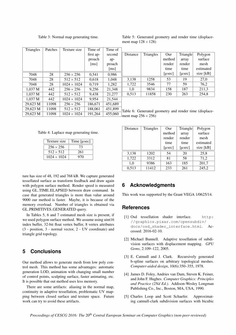
Table 3: Normal map generating time.
Triangles Patches Texture size Time offirst ap-proach[ms]
Time ofsecond
ap-proach[ms]
7048 28 256×256 0,541 0,9867048 28 512×512 0,618 1,0487048 28 1024×1024 0,719 1,282
1,037 M 442 256×256 9,256 21,3481,037 M 442 512×512 9,438 21,2771,037 M 442 1024×1024 9,954 21,544
29,623 M 11098 256×256 186,671 451,68929,623 M 11098 512×512 188,061 451,89929,623 M 11098 1024×1024 191,264 455,060
Table 4: Laplace map generating time.
Texture size Time [µsec]256×256 73512×512 261
1024×1024 970
ture has size of 48, 192 and 768 kB. We capture generatedtessellated surface as transform feedback and draw againwith polygon surface method. Render speed is measuredusing GL TIME ELAPSED between draw command. Incase that generated triangles is more than value around9000 our method is faster. Maybe, it is because of thememory overload. Number of triangles is obtained viaGL PRIMITIVES GENERATED query.
In Tables 5, 6 and 7 estimated mesh size is present, ifwe used polygon surface method. We assume using uint16index buffer, 32-bit float vertex buffer, 8 vertex attributes(3 - position, 3 - normal vector, 2 - UV coordinate) andtriangle grid topology.
5 Conclusions
Our method allows to generate mesh from low poly con-trol mesh. This method has some advantages: automaticgeneration LOD, animation with changing small numberof control points, sculpting surface, faster animating, etc.It is possible that out method uses less memory.
There are some artifacts: aliasing in the normal map,continuity in adaptive tessellation, problematic UV map-ping between closed surface and texture space. Futurework can try to avoid these artifacts.
Table 5: Generated geometry and render time (displace-ment map 128×128)
Distance Triangles Ourmethodrendertime
[µsec]
Trianglearray
rendertime
[µsec]
Polygonsurfacemesh
estimatedsize [kB]
3,138 1258 53 19 27,01,722 3546 77 59 76,21,0 9834 158 187 211,3
0,513 11858 230 263 254,8
Table 6: Generated geometry and render time (displace-ment map 256×256)
Distance Triangles Ourmethodrendertime
[µsec]
Trianglearray
rendertime
[µsec]
Polygonsurfacemesh
estimatedsize [kB]
3,138 1202 54 20 25,81,722 3312 81 58 71,21,0 9386 163 185 201,7
0,513 11412 233 261 245,2
6 Acknowledgments
This work was supported by the Grant VEGA 1/0625/14.
References
[1] Osd tessellation shader interface. http://graphics.pixar.com/opensubdiv/docs/osd_shader_interface.html. Ac-cessed: 2016-02-10.
[2] Michael Bunnell. Adaptive tessellation of subdi-vision surfaces with displacement mapping. GPUGems, 2:109–122, 2005.
[3] E. Catmull and J. Clark. Recursively generatedb-spline surfaces on arbitrary topological meshes.Computer-aided design, 10(6):350–355, 1978.
[4] James D. Foley, Andries van Dam, Steven K. Feiner,and John F. Hughes. Computer Graphics: Principlesand Practice (2Nd Ed.). Addison-Wesley LongmanPublishing Co., Inc., Boston, MA, USA, 1990.
[5] Charles Loop and Scott Schaefer. Approximat-ing catmull-clark subdivision surfaces with bicubic
Proceedings of CESCG 2016: The 20th Central European Seminar on Computer Graphics (non-peer-reviewed)
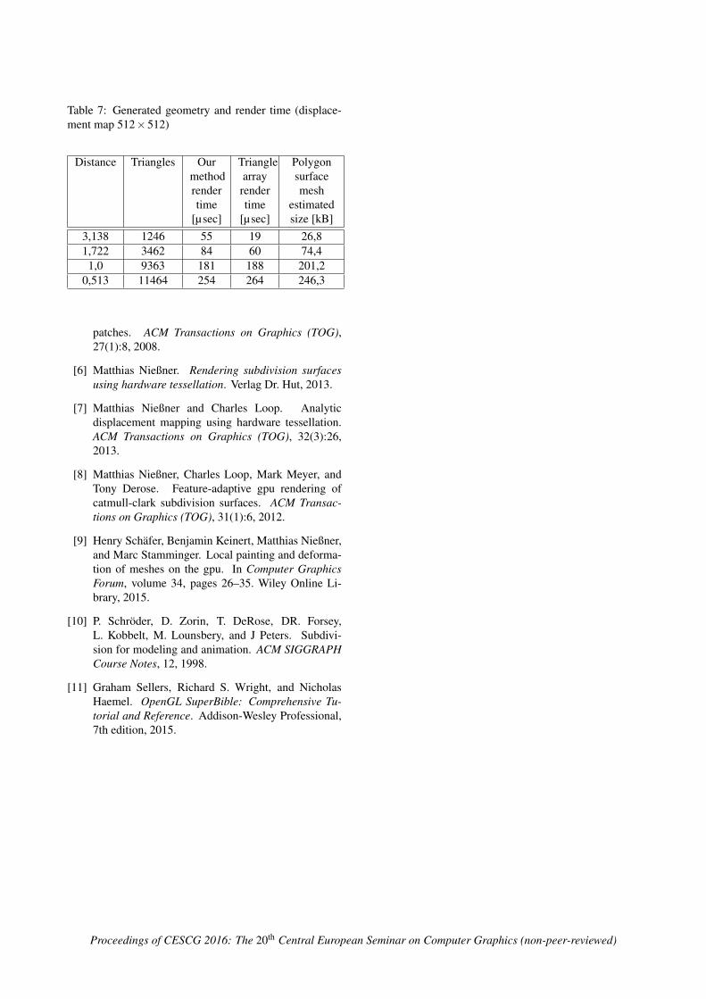
Table 7: Generated geometry and render time (displace-ment map 512×512)
Distance Triangles Ourmethodrendertime
[µsec]
Trianglearray
rendertime
[µsec]
Polygonsurfacemesh
estimatedsize [kB]
3,138 1246 55 19 26,81,722 3462 84 60 74,4
1,0 9363 181 188 201,20,513 11464 254 264 246,3
patches. ACM Transactions on Graphics (TOG),27(1):8, 2008.
[6] Matthias Nießner. Rendering subdivision surfacesusing hardware tessellation. Verlag Dr. Hut, 2013.
[7] Matthias Nießner and Charles Loop. Analyticdisplacement mapping using hardware tessellation.ACM Transactions on Graphics (TOG), 32(3):26,2013.
[8] Matthias Nießner, Charles Loop, Mark Meyer, andTony Derose. Feature-adaptive gpu rendering ofcatmull-clark subdivision surfaces. ACM Transac-tions on Graphics (TOG), 31(1):6, 2012.
[9] Henry Schafer, Benjamin Keinert, Matthias Nießner,and Marc Stamminger. Local painting and deforma-tion of meshes on the gpu. In Computer GraphicsForum, volume 34, pages 26–35. Wiley Online Li-brary, 2015.
[10] P. Schroder, D. Zorin, T. DeRose, DR. Forsey,L. Kobbelt, M. Lounsbery, and J Peters. Subdivi-sion for modeling and animation. ACM SIGGRAPHCourse Notes, 12, 1998.
[11] Graham Sellers, Richard S. Wright, and NicholasHaemel. OpenGL SuperBible: Comprehensive Tu-torial and Reference. Addison-Wesley Professional,7th edition, 2015.
Proceedings of CESCG 2016: The 20th Central European Seminar on Computer Graphics (non-peer-reviewed)