Rendered Path: Range-Free Localization in Anisotropic Sensor Networks with Holes

Mo Li, Yunhao Liu 973 WSN Joint Lab

Hong Kong University of Science and Technology {limo, liu}@cse.ust.hk

ABSTRACT Sensor positioning is a crucial part of many location-dependent applications that utilize wireless sensor networks (WSNs). Current localization approaches can be divided into two groups: range-based and range-free. Due to the high costs and critical as-sumptions, the range-based schemes are often impractical for WSNs. The existing range-free schemes, on the other hand, suffer from poor accuracy and low scalability. Without the help of a large number of uniformly deployed seed nodes, those schemes fail in anisotropic WSNs with possible holes. To address this issue, we propose the Rendered Path (REP) protocol. To the best of our knowledge, REP is the only range-free protocol for locating sen-sors with constant number of seeds in anisotropic sensor net-works.

Categories and Subject Descriptors C.2.1 [Computer Communication Networks]: Network Architecture and Design – Distributed networks; Wireless communication; C.2.4 [Computer Communication Networks]: Distributed Systems - Dis-tributed applications; E.1 [Data]: Data Structures – Graph and net-works.

General Terms Algorithms, Design, Theory

Keywords Wireless Sensor Network; Range-free; Localization; Anisotropic

1. INTRODUCTION The ability to automatically locate sensor nodes is essential in many WSN applications. The current approaches for this mainly fall into two categories: range-based and range-free [9]. Range-based approaches assume that sensor nodes are able to measure the distances, or even relative directions of their neighbor nodes, based on Time of Arrival (TOA) [25], Time Difference of Arrival (TDOA) [19], Radio Signal Strength (RSS) [1] or Angle of Arrival (AOA) [17], etc. Such assumptions are critical, introduc-ing extra requirements and costs to the hardware design of sensor node devices. Furthermore, in many practical situations, the meas-

urements are far from accurate (and even sometimes unobtainable) due to highly dynamic environments. In order to address this issue, many range-free approaches have been proposed. These ap-proaches do not require sensors to have special hardware func-tionalities, and each senor can merely know the existence of its neighbor nodes.

Range-free localization techniques are considered more cost-effective and less limited for a wider range of applications in WSNs than range-based techniques. To truly adopt range-free approaches, however, many challenges need to be addressed. Since there is no way to measure physical distances between nodes, existing approaches depend largely on connectivity-based algo-rithms, setting a tradeoff between the accuracy and the number of location-equipped seed nodes [4] needed as referees. The draw-backs of such approaches are obvious. To accurately localize the undetermined nodes, the number of seeds needs to be proportional to the network size. Also, the seeds need to be uniformly deployed [4, 9, 11, 13], and many approaches assume that seed nodes have radio ranges that are ten times larger than those of normal nodes. In [9], to obtain an estimation error below the node radio range R, each undetermined node must hear at least 7 seeds as referees on average. To our knowledge, in sensor networks, DV-hop [18] is the only approach which employs a constant number of seeds, but it relies on the heuristic of proportionality between the Euclidean distance and hop count in isotropic networks. The system esti-mates the average distance per hop from seed locations and the hop count among seeds.

Most previous approaches would fail in anisotropic networks, where holes exist among sensor nodes. In anisotropic networks, the Euclidean distances between a pair of nodes may not correlate closely with the hop counts between them because the path be-tween them may have to curve around intermediate holes. Thus, the proportionality heuristic [18] no longer holds. Indeed, anisot-ropic networks are more likely to exist in practice for several rea-sons. First, in many real applications, sensor nodes/seeds can rarely be uniformly deployed over the field due to the geographi-cal obstacles. Second, even if we assume that the initial sensor network is isotropic, unbalanced power consumption among nodes will likely create holes in the network. Last, events such as exter-nal interference may cause communication failures which result in holes in the network. Some space embedding approaches [13, 21] enable the localization in anisotropic networks. However, they all imply the critical assumption that a percentage of seed nodes are uniformly deployed over the network.

In this work, we propose REndered Path (REP) protocol, a range-free scheme for locating sensors in anisotropic WSNs with holes. By path rendering and virtual hole construction operations in a distributed manner, REP is able to accurately estimate the

Permission to make digital or hard copies of all or part of this work for personal or classroom use is granted without fee provided that copies are not made or distributed for profit or commercial advantage and that copies bear this notice and the full citation on the first page. To copy otherwise, or republish, to post on servers or to redistribute to lists, requires prior specific permission and/or a fee. MobiCom’07, September 9–14, 2007, Montreal, Quebec, Canada. Copyright 2007 ACM 978-1-59593-681-3/07/0009...$5.00.

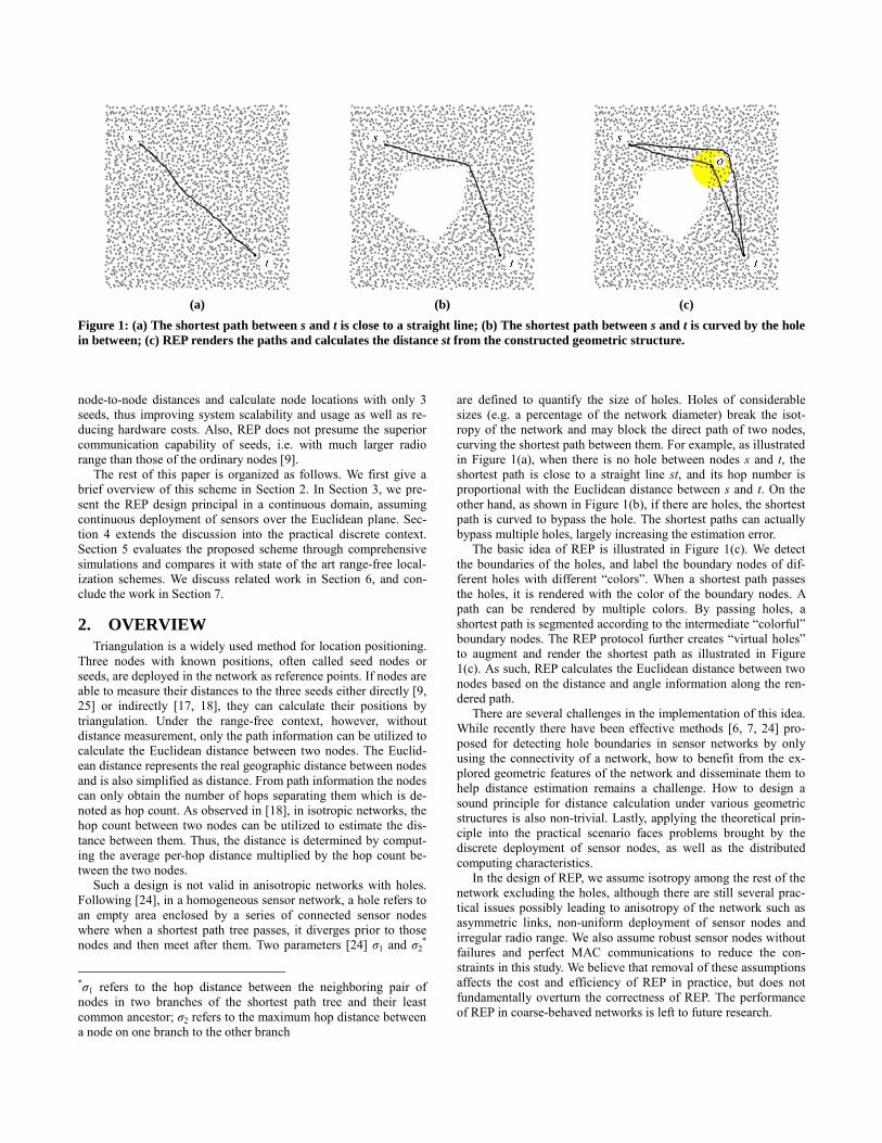
(a) (b) (c)

Figure 1: (a) The shortest path between s and t is close to a straight line; (b) The shortest path between s and t is curved by the hole in between; (c) REP renders the paths and calculates the distance st from the constructed geometric structure.

node-to-node distances and calculate node locations with only 3 seeds, thus improving system scalability and usage as well as re-ducing hardware costs. Also, REP does not presume the superior communication capability of seeds, i.e. with much larger radio range than those of the ordinary nodes [9].

The rest of this paper is organized as follows. We first give a brief overview of this scheme in Section 2. In Section 3, we pre-sent the REP design principal in a continuous domain, assuming continuous deployment of sensors over the Euclidean plane. Sec-tion 4 extends the discussion into the practical discrete context. Section 5 evaluates the proposed scheme through comprehensive simulations and compares it with state of the art range-free local-ization schemes. We discuss related work in Section 6, and con-clude the work in Section 7.

2. OVERVIEW Triangulation is a widely used method for location positioning. Three nodes with known positions, often called seed nodes or seeds, are deployed in the network as reference points. If nodes are able to measure their distances to the three seeds either directly [9, 25] or indirectly [17, 18], they can calculate their positions by triangulation. Under the range-free context, however, without distance measurement, only the path information can be utilized to calculate the Euclidean distance between two nodes. The Euclid-ean distance represents the real geographic distance between nodes and is also simplified as distance. From path information the nodes can only obtain the number of hops separating them which is de-noted as hop count. As observed in [18], in isotropic networks, the hop count between two nodes can be utilized to estimate the dis-tance between them. Thus, the distance is determined by comput-ing the average per-hop distance multiplied by the hop count be-tween the two nodes.

Such a design is not valid in anisotropic networks with holes. Following [24], in a homogeneous sensor network, a hole refers to an empty area enclosed by a series of connected sensor nodes where when a shortest path tree passes, it diverges prior to those nodes and then meet after them. Two parameters [24] σ1 and σ2

*

*σ1 refers to the hop distance between the neighboring pair of nodes in two branches of the shortest path tree and their least common ancestor; σ2 refers to the maximum hop distance between a node on one branch to the other branch

are defined to quantify the size of holes. Holes of considerable sizes (e.g. a percentage of the network diameter) break the isot-ropy of the network and may block the direct path of two nodes, curving the shortest path between them. For example, as illustrated in Figure 1(a), when there is no hole between nodes s and t, the shortest path is close to a straight line st, and its hop number is proportional with the Euclidean distance between s and t. On the other hand, as shown in Figure 1(b), if there are holes, the shortest path is curved to bypass the hole. The shortest paths can actually bypass multiple holes, largely increasing the estimation error.

The basic idea of REP is illustrated in Figure 1(c). We detect the boundaries of the holes, and label the boundary nodes of dif-ferent holes with different “colors”. When a shortest path passes the holes, it is rendered with the color of the boundary nodes. A path can be rendered by multiple colors. By passing holes, a shortest path is segmented according to the intermediate “colorful” boundary nodes. The REP protocol further creates “virtual holes” to augment and render the shortest path as illustrated in Figure 1(c). As such, REP calculates the Euclidean distance between two nodes based on the distance and angle information along the ren-dered path.

There are several challenges in the implementation of this idea. While recently there have been effective methods [6, 7, 24] pro-posed for detecting hole boundaries in sensor networks by only using the connectivity of a network, how to benefit from the ex-plored geometric features of the network and disseminate them to help distance estimation remains a challenge. How to design a sound principle for distance calculation under various geometric structures is also non-trivial. Lastly, applying the theoretical prin-ciple into the practical scenario faces problems brought by the discrete deployment of sensor nodes, as well as the distributed computing characteristics.

In the design of REP, we assume isotropy among the rest of the network excluding the holes, although there are still several prac-tical issues possibly leading to anisotropy of the network such as asymmetric links, non-uniform deployment of sensor nodes and irregular radio range. We also assume robust sensor nodes without failures and perfect MAC communications to reduce the con-straints in this study. We believe that removal of these assumptions affects the cost and efficiency of REP in practice, but does not fundamentally overturn the correctness of REP. The performance of REP in coarse-behaved networks is left to future research.

α αθ

(a) (b) (a) (b)

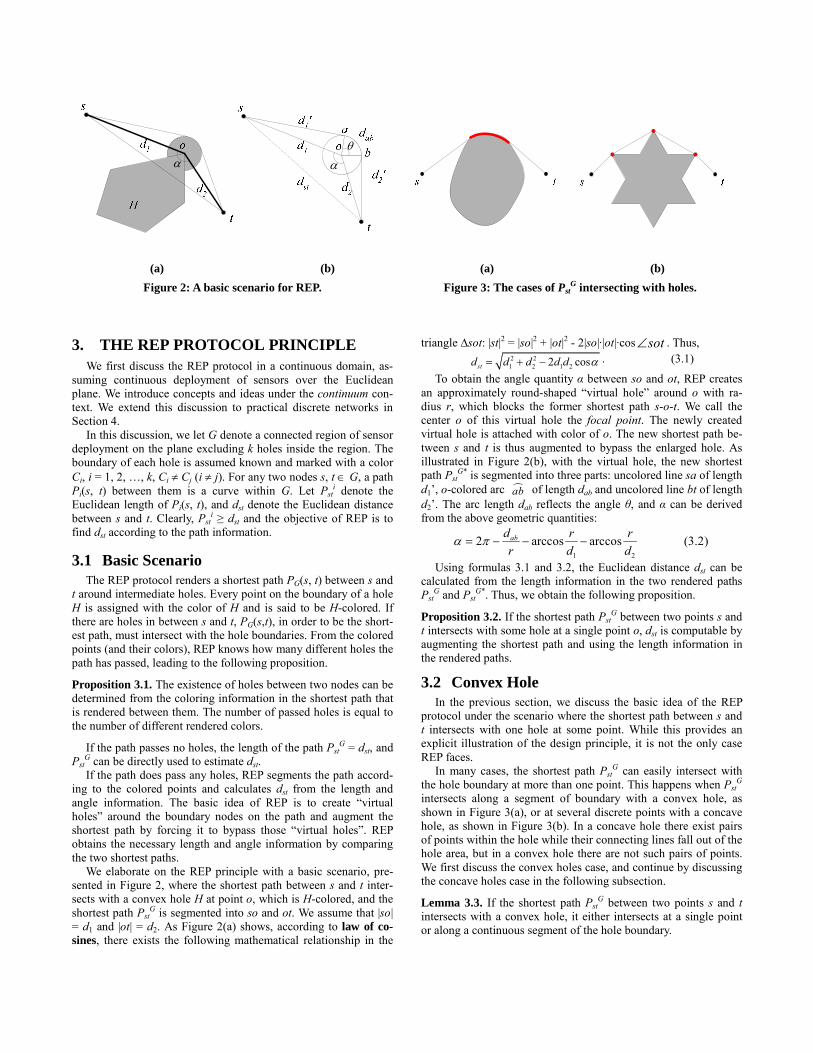
Figure 2: A basic scenario for REP. Figure 3: The cases of PstG intersecting with holes.

3. THE REP PROTOCOL PRINCIPLE We first discuss the REP protocol in a continuous domain, as-

suming continuous deployment of sensors over the Euclidean plane. We introduce concepts and ideas under the continuum con-text. We extend this discussion to practical discrete networks in Section 4.

In this discussion, we let G denote a connected region of sensor deployment on the plane excluding k holes inside the region. The boundary of each hole is assumed known and marked with a color Ci, i = 1, 2, …, k, Ci ≠ Cj (i ≠ j). For any two nodes s, t ∈ G, a path Pi(s, t) between them is a curve within G. Let Pst

i denote the Euclidean length of Pi(s, t), and dst denote the Euclidean distance between s and t. Clearly, Pst

i ≥ dst and the objective of REP is to find dst according to the path information.

3.1 Basic Scenario The REP protocol renders a shortest path PG(s, t) between s and t around intermediate holes. Every point on the boundary of a hole H is assigned with the color of H and is said to be H-colored. If there are holes in between s and t, PG(s,t), in order to be the short-est path, must intersect with the hole boundaries. From the colored points (and their colors), REP knows how many different holes the path has passed, leading to the following proposition.

Proposition 3.1. The existence of holes between two nodes can be determined from the coloring information in the shortest path that is rendered between them. The number of passed holes is equal to the number of different rendered colors.

If the path passes no holes, the length of the path PstG = dst, and

PstG can be directly used to estimate dst.

If the path does pass any holes, REP segments the path accord-ing to the colored points and calculates dst from the length and angle information. The basic idea of REP is to create “virtual holes” around the boundary nodes on the path and augment the shortest path by forcing it to bypass those “virtual holes”. REP obtains the necessary length and angle information by comparing the two shortest paths. We elaborate on the REP principle with a basic scenario, pre-sented in Figure 2, where the shortest path between s and t inter-sects with a convex hole H at point o, which is H-colored, and the shortest path Pst

G is segmented into so and ot. We assume that |so| = d1 and |ot| = d2. As Figure 2(a) shows, according to law of co-sines, there exists the following mathematical relationship in the

triangle ∆sot: |st|2 = |so|2 + |ot|2 - 2|so|·|ot|·cos sot∠ . Thus, 2 2

1 2 1 22 cosstd d d d d α= + − . (3.1)

To obtain the angle quantity α between so and ot, REP creates an approximately round-shaped “virtual hole” around o with ra-dius r, which blocks the former shortest path s-o-t. We call the center o of this virtual hole the focal point. The newly created virtual hole is attached with color of o. The new shortest path be-tween s and t is thus augmented to bypass the enlarged hole. As illustrated in Figure 2(b), with the virtual hole, the new shortest path Pst

G* is segmented into three parts: uncolored line sa of length d1’, o-colored arc ab of length dab and uncolored line bt of length d2’. The arc length dab reflects the angle θ, and α can be derived from the above geometric quantities:

1 2

2 arccos arccos (3.2)abd r rr d d

α π= − − −

Using formulas 3.1 and 3.2, the Euclidean distance dst can be calculated from the length information in the two rendered paths Pst

G and PstG*. Thus, we obtain the following proposition.

Proposition 3.2. If the shortest path PstG between two points s and

t intersects with some hole at a single point o, dst is computable by augmenting the shortest path and using the length information in the rendered paths.

3.2 Convex Hole In the previous section, we discuss the basic idea of the REP protocol under the scenario where the shortest path between s and t intersects with one hole at some point. While this provides an explicit illustration of the design principle, it is not the only case REP faces. In many cases, the shortest path Pst

G can easily intersect with the hole boundary at more than one point. This happens when Pst

G intersects along a segment of boundary with a convex hole, as shown in Figure 3(a), or at several discrete points with a concave hole, as shown in Figure 3(b). In a concave hole there exist pairs of points within the hole while their connecting lines fall out of the hole area, but in a convex hole there are not such pairs of points. We first discuss the convex holes case, and continue by discussing the concave holes case in the following subsection.

Lemma 3.3. If the shortest path PstG between two points s and t

intersects with a convex hole, it either intersects at a single point or along a continuous segment of the hole boundary.

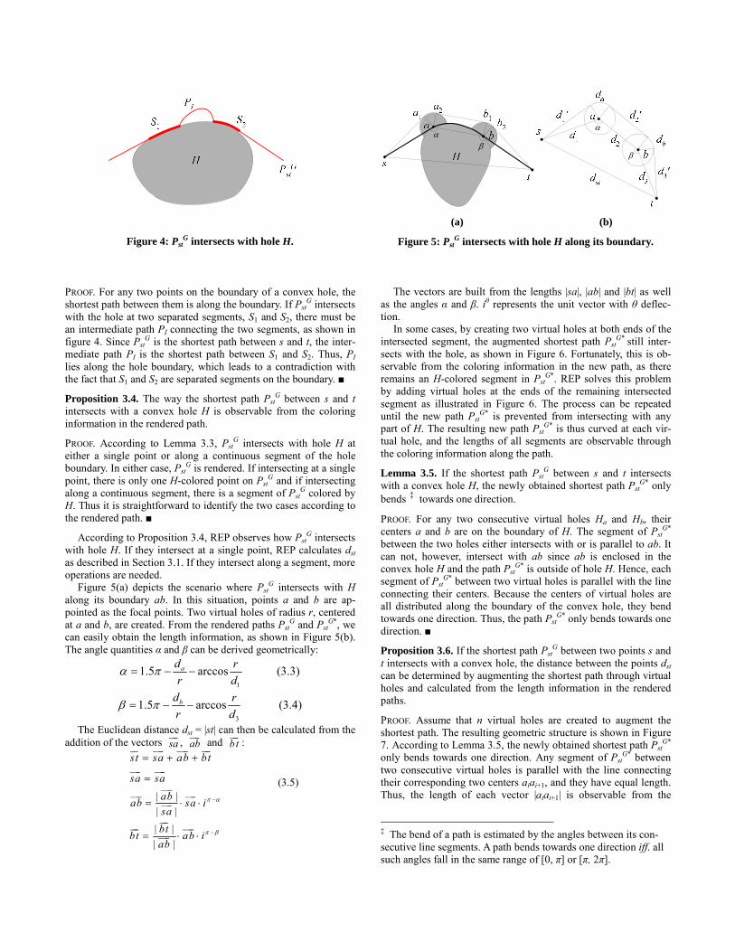
Figure 4: PstG intersects with hole H.

PROOF. For any two points on the boundary of a convex hole, the shortest path between them is along the boundary. If Pst

G intersects with the hole at two separated segments, S1 and S2, there must be an intermediate path PI connecting the two segments, as shown in figure 4. Since Pst

G is the shortest path between s and t, the inter-mediate path PI is the shortest path between S1 and S2. Thus, PI lies along the hole boundary, which leads to a contradiction with the fact that S1 and S2 are separated segments on the boundary. ■

Proposition 3.4. The way the shortest path PstG between s and t

intersects with a convex hole H is observable from the coloring information in the rendered path.

PROOF. According to Lemma 3.3, PstG intersects with hole H at

either a single point or along a continuous segment of the hole boundary. In either case, Pst

G is rendered. If intersecting at a single point, there is only one H-colored point on Pst

G and if intersecting along a continuous segment, there is a segment of Pst

G colored by H. Thus it is straightforward to identify the two cases according to the rendered path. ■

According to Proposition 3.4, REP observes how PstG intersects

with hole H. If they intersect at a single point, REP calculates dst as described in Section 3.1. If they intersect along a segment, more operations are needed. Figure 5(a) depicts the scenario where Pst

G intersects with H along its boundary ab. In this situation, points a and b are ap-pointed as the focal points. Two virtual holes of radius r, centered at a and b, are created. From the rendered paths Pst

G and PstG*, we

can easily obtain the length information, as shown in Figure 5(b). The angle quantities α and β can be derived geometrically:

1

1.5 arccos (3.3)ad rr d

α π= − −

3

1.5 arccos (3.4)bd rr d

β π= − −

The Euclidean distance dst = |st| can then be calculated from the addition of the vectors sa , ab and bt : st sa ab bt= + +

| || || || |

sa sa

abab sa isabtbt ab iab

π α

π β

−

−

=

= ⋅ ⋅

= ⋅ ⋅

(3.5)

β

αβ

α

(a) (b)

Figure 5: PstG intersects with hole H along its boundary.

The vectors are built from the lengths |sa|, |ab| and |bt| as well as the angles α and β. iθ represents the unit vector with θ deflec-tion. In some cases, by creating two virtual holes at both ends of the intersected segment, the augmented shortest path Pst

G* still inter-sects with the hole, as shown in Figure 6. Fortunately, this is ob-servable from the coloring information in the new path, as there remains an H-colored segment in Pst

G*. REP solves this problem by adding virtual holes at the ends of the remaining intersected segment as illustrated in Figure 6. The process can be repeated until the new path Pst

G* is prevented from intersecting with any part of H. The resulting new path Pst

G* is thus curved at each vir-tual hole, and the lengths of all segments are observable through the coloring information along the path.

Lemma 3.5. If the shortest path PstG between s and t intersects

with a convex hole H, the newly obtained shortest path PstG* only

bends ‡ towards one direction.

PROOF. For any two consecutive virtual holes Ha and Hb, their centers a and b are on the boundary of H. The segment of Pst

G* between the two holes either intersects with or is parallel to ab. It can not, however, intersect with ab since ab is enclosed in the convex hole H and the path Pst

G* is outside of hole H. Hence, each segment of Pst

G* between two virtual holes is parallel with the line connecting their centers. Because the centers of virtual holes are all distributed along the boundary of the convex hole, they bend towards one direction. Thus, the path Pst

G* only bends towards one direction. ■

Proposition 3.6. If the shortest path PstG between two points s and

t intersects with a convex hole, the distance between the points dst can be determined by augmenting the shortest path through virtual holes and calculated from the length information in the rendered paths.

PROOF. Assume that n virtual holes are created to augment the shortest path. The resulting geometric structure is shown in Figure 7. According to Lemma 3.5, the newly obtained shortest path Pst

G* only bends towards one direction. Any segment of Pst

G* between two consecutive virtual holes is parallel with the line connecting their corresponding two centers aiai+1, and they have equal length. Thus, the length of each vector |aiai+1| is observable from the

‡ The bend of a path is estimated by the angles between its con-secutive line segments. A path bends towards one direction iff. all such angles fall in the same range of [0, π] or [π, 2π].

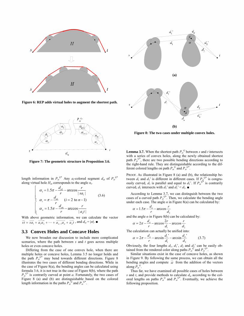
Figure 6: REP adds virtual holes to augment the shortest path.

1α

2α 1nα −

nα

Figure 7: The geometric structure in Proposition 3.6.

length information in Pst

G* Any ai-colored segment dai of PstG*

along virtual hole Hai corresponds to the angle αi.

11

1

1.5 arccos| |

( 2 to 1)

1.5 arccos| |

a

aii

ann

n

d rr sa

d i nr

d rr a t

α π

α π

α π

⎧ = − −⎪⎪⎪ = − = −⎨⎪⎪ = − −⎪⎩

(3.6)

With above geometric information, we can calculate the vector

1 1 2 1n n nst sa a a a a a t−= + + + + , and dst = |st|. ■

3.3 Convex Holes and Concave Holes We now broaden our discussion to include more complicated scenarios, where the path between s and t goes across multiple holes or even concave holes. Differing from the case of one convex hole, when there are multiple holes or concave holes, Lemma 3.5 no longer holds and the path Pst

G* may bend towards different directions. Figure 8 illustrates the two cases of different bending directions. While in the case of Figure 8(a), the bending angles can be calculated using formula 3.6, it is not true in the case of Figure 8(b), where the path Pst

G* is contrarily curved at point a. Fortunately, the two cases of Figure 8 (a) and (b) are distinguishable based on the colored length information in the paths Pst

G and PstG*.

α

(a)

α

(b)

Figure 8: The two cases under multiple convex holes.

Lemma 3.7. When the shortest path PstG between s and t intersects

with a series of convex holes, along the newly obtained shortest path Pst

G*, there are two possible bending directions according to the right-hand rule. They are distinguishable according to the dif-ferent colored lengths on path Pst

G and PstG*.

PROOF. As illustrated in Figure 8 (a) and (b), the relationship be-tween d1 and d1’ is different in different cases. If Pst

G* is congru-ously curved, d1 is parallel and equal to d1’. If Pst

G* is contrarily curved, d1 intersects with d1’ and d1’ < d1. ■

According to Lemma 3.7, we can distinguish between the two cases of a curved path Pst

G*. Then, we calculate the bending angle under each case. The angle α in Figure 8(a) can be calculated by:

2

1.5 arccosad rr d

α π= − −

and the angle α in Figure 8(b) can be calculated by:

1 2

22 arccos arccosad r rr d d

α π= − − −

The calculation can actually be unified into: 1 2

1 2

' '2 arcsin arcsin (3.7)ad d dr d d

α π= − − −

Obviously, the four lengths d1, d1’, d2 and d2’ can be easily ob-tained from the rendered color along paths Pst

G and PstG*.

Similar situations exist in the case of concave holes, as shown in Figure 9. By following the same process, we can obtain all the bending angles and compute st from the addition of the vectors along Pst

G. Thus far, we have examined all possible cases of holes between s and t, and provide methods to calculate dst according to the col-ored lengths on paths Pst

G and PstG*. Eventually, we achieve the

following proposition.

(a) (b)

Figure 9: The two cases under concave holes.

Proposition 3.8. The distance dst between any two points s and t is computable from the length information in the paths rendered between them.

4 THE REP PROTOCOL IN PRACTICE We have described the principle of the REP protocol in the continuous domain. In a real deployed sensor network, however, sensors are distributed discretely on the field. Also, due to the lack of global coordination, the methods of coloring the nodes, render-ing the paths, and disseminating the coloring information in a distributed manner need to be addressed. In the range-free context, each sensor node only detects the existence of its neighbors. This means that we do not have the distances so that the REP protocol needs to be fine-tuned in order to minimize the errors in deriving the Euclidean distances from the hop count. Note that we only assume three location-equipped seeds are distributed throughout the network.

The practical REP protocol includes five major components: boundary detection, shortest path exploration, virtual hole con-struction, virtual shortest path construction, and distance comput-ing. The protocol proceeds as follows. First, the system detects and enumerates the holes inside the hole boundary as well as the nodes on the boundary using the algorithm in [24]. Then, each node explores the shortest path to the three seeds and calculates the Euclidean distances to them by rendering and augmenting the shortest paths. Based on the estimated distances to the seeds, the nodes localize themselves by triangulation. All operations are carried out in a distributed fashion among discrete sensor nodes. We present the details of the five REP components in the rest of this section.

4.1 Boundary Detection In this component, REP detects the boundaries of holes. Each hole is enumerated and attached with an ID. Each boundary node belongs to a certain hole and is tagged with the hole ID. There have been many algorithms proposed to detect and distinguish the nodes on hole boundaries in sensor networks by only using the connectivity of a network [6, 7]. A recently proposed algorithm [24] elegantly detects all boundaries, groups the boundary nodes, and connects them into meaningful boundaries for each hole. We can directly use the design in [24] to enumerate the holes and color the boundary nodes with each hole ID. After boundary detection, each boundary node Vi in the network is detected and it allocates a space to store its color CH, i.e. its corresponding hole ID H(Vi). The ordinary nodes will not be labeled with any color or hole ID.

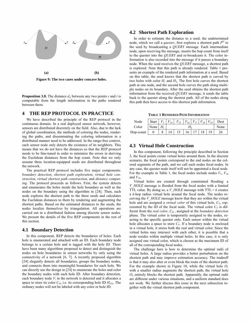
4.2 Shortest Path Exploration In order to estimate the distance to a seed, the undetermined node, which we call a quester, first explores a shortest path PG to the seed by broadcasting a QUERY message. Each intermediate node, upon receiving the message, inserts the hop count from itself to the quester into the QUERY and re-broadcasts it. The color in-formation is also recorded into the message if it passes a boundary node. When the seed receives the QUERY message, a shortest path is explored. Note that this path is already rendered. Table 1 pre-sents an example of the rendered path information at a seed. Based on this table, the seed knows that the shortest path is curved by two holes with color H1 and H2. The first hole curves the shortest path at one node, and the second hole curves the path along multi-ple nodes on its boundary. After the seed obtains the shortest path information from the received QUERY message, it sends the table back to the quester along the shortest path. All of the nodes along this path then have access to this shortest path information.

TABLE 1 RENDERED PATH INFORMATION

Node Start V1 V14 V15 V16 V17 V18 V19 DestColor None H1 H2 None

Hop-count 0 8 14 15 16 17 18 19 26

4.3 Virtual Hole Construction In this component, following the principle described in Section

3, the focal points create virtual holes around them. In the discrete scenario, the focal points correspond to the end nodes on the col-ored segments of the path, and we call such nodes focal nodes. In any case, the quester node itself will not be appointed a focal node. For the example in Table 1, the focal nodes include nodes V1, V14 and V19.

Virtual holes are created through constrained flooding: a V_HOLE message is flooded from the focal nodes with a limited TTL value. By doing so, a V_HOLE message with TTL = k creates a k-hop radius virtual hole around the focal node. The nodes re-ceiving the V_HOLE message know that they are within the virtual hole and are assigned a virtual color of this virtual hole, CV, rep-resented by the ID of the focal node. The virtual color CV is dif-ferent from the real color, CH , assigned at the boundary detection phase. The virtual color is temporarily assigned to the nodes, re-acting to the specific quester only. Each sensor within the virtual hole allocates a space to store CV. If a boundary node is enclosed in a virtual hole, it stores both the real and virtual color. Since the virtual holes may intersect with each other, it is possible that a node resides within multiple virtual holes. In this case, it is only assigned one virtual color, which is chosen as the maximum ID of all of the corresponding focal nodes.

The challenge here is how to determine the optimal radii of virtual holes. A large radius provides a better perturbation on the shortest path and may improve estimation accuracy. The tradeoff is that it may also alter or even block the route of the shortest path. For the example shown in Figure 10, while the virtual hole O1 with a smaller radius augments the shortest path, the virtual hole O2 entirely blocks the shortest path. Apparently, the optimal radii are different under various situations, and a uniform standard does not work. We further discuss this issue in the next subsection to-gether with the virtual shortest path component.

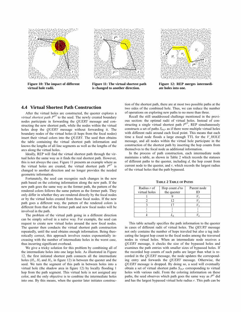
Figure 10: The impact of different virtual hole radii.

Figure 11: The virtual shortest path is changed to another direction.

Figure 12: REP merges intermedi-ate holes into one.

4.4 Virtual Shortest Path Construction After the virtual holes are constructed, the quester explores a

virtual shortest path PG* to the seed. The newly created boundary nodes participate in forwarding the QUERY message and con-structing the new shortest path, while the nodes within the virtual holes drop the QUERY message without forwarding it. The boundary nodes of the virtual holes (k hops from the focal nodes) insert their virtual colors into the QUERY. The seed then obtains the table containing the virtual shortest path information and knows the lengths of all line segments as well as the lengths of the arcs along the virtual holes.

Ideally, REP will find the virtual shortest path through the vir-tual holes the same way as it finds the real shortest path. However, this is not always the case. Figure 11 presents an example where as the virtual holes are created, the virtual shortest path PG* is changed to another direction and no longer provides the needed geometric information.

Fortunately, the seed can recognize such changes in the new path based on the coloring information along the new path. If the new path goes the same way as the former path, the pattern of the rendered colors follows the same pattern as the former path. They only differ in whether they are rendered directly by the focal nodes or by the virtual holes created from those focal nodes. If the new path goes a different way, the pattern of the rendered colors is different from that of the former path and new focal nodes will be involved in the path.

The problem of the virtual path going in a different direction can be simply solved in a naïve way. For example, the seed can request to create new virtual holes around the new focal nodes. The quester then conducts the virtual shortest path construction repeatedly, until the seed obtains enough information. Being theo-retically correct, this approach involves routes exponentially in-creasing with the number of intermediate holes in the worst case, thus incurring significant overhead.

We give a tricky solution for this problem by combining all of the intermediate holes into one large hole. As illustrated in Figure 12, the first initiated shortest path connects all the intermediate holes (H1, H2 and H3, in figure 12) in between the quester and the seed. We turn the segment of this path in between holes into a virtual hole (the shadow area in figure 12) by locally flooding 1 hop from the path segment. This virtual hole is not assigned any color, and the only objective is to combine the intermediate holes into one. By this means, when the quester later initiates construc-

tion of the shortest path, there are at most two possible paths at the two sides of the combined hole. Thus, we can reduce the number of operations on exploring new paths to no more than three.

Recall the still unaddressed challenge mentioned in the previ-ous section: the optimal radii of virtual holes. Instead of con-structing a single virtual shortest path PG*, REP simultaneously constructs a set of paths SPG* as if there were multiple virtual holes with different radii around each focal point. This means that each time a focal node floods a large enough TTL for the V_HOLE message, and all nodes within the virtual hole participate in the construction of the shortest path by inserting the hop counts from themselves to the focal node as additional information.

In the process of path construction, each intermediate node maintains a table, as shown in Table 2 which records the statuses of different paths to the quester, including d, the hop count from current node to the quester, and r, which records the largest radius of the virtual holes that the path bypassed.

TABLE 2 TABLE OF PATHS

Radius r of virtual holes

Hop count d to the quester

Parent node ID

1 9 V1 2 12 V2 3 17 V3

k Lk Vk

This table actually specifies the path information to the quester in cases of different radii of virtual holes. The QEURY message not only contains the number of hops traveled but also a tag indi-cating the largest hop count to the focal nodes among the traversed nodes in virtual holes. When an intermediate node receives a QUERY message, it checks the size of the bypassed holes and examines the path entries with smaller sizes of bypassed holes. If the recorded hop counts of such paths are larger than what is re-corded in the QUERY message, the node updates the correspond-ing entry and forwards the QUERY message. Otherwise, the QUERY message is dropped. By doing so, a seed will eventually obtain a set of virtual shortest paths SPG* corresponding to virtual holes with various radii. From the coloring information on these paths, the seed observes which path goes the same way as PG did and has the largest bypassed virtual hole radius r. This path can be

appointed as PG* and used to calculate the distance with mini-mized error. Such an operation is equivalent to dynamically tuning the optimized radii of virtual holes, but in a distributed and con-current manner. The process is accomplished in one turn of flood-ing.

4.5 Distance Computing Using the two rendered paths, the real and the virtual shortest

paths, a seed can calculate the direct distance to the quester based on the principle described in Section 3. The seed then delivers this distance value to the quester along the path PG. The delivery also triggers focal nodes to eliminate the virtual holes by locally flood-ing the V_HOLE_ELIMINATE messages. Note that in this stage the distance between the seed and quester is represented in terms of hop counts, while what we need is the physical distance. Since we assume no ranging capability of each node, there is no direct way to map the hop count to the Euclidean distance. We address this issue by first computing the hop count of the direct way be-tween each pair of seeds, using REP protocol. Since the Euclidean distances between seeds are known, we can then estimate the av-erage length of each hop by comparing the two types of distances. Using the three Euclidean distances from the seeds, a quester can then easily compute its location by triangulation.

4.6 Further Discussion For simplicity, in previous discussions, we assume that the REP scheme is sequentially carried out. Each time, one node holds global resources for calculating the distances to the three seeds. This significantly limits the efficiency and scalability of the pro-tocol. In the implementation, we can use the pairing of a seed and a quester’s node ID as an identifier and attach it to the corre-sponding paths. This identifier is used to mark the concerned par-ties participating in the interactive operations, and is disseminated to the corresponding virtual holes created along the first generated shortest path PG. In the following operations, all participating parties limit their actions within the local domain under this iden-tifier. The virtual holes only render the paths with the same identi-fier. One node may belong to multiple local domains and acts dif-ferently for different identifiers according to its role in each do-main. By doing so, multiple nodes may initiate their queries si-multaneously under different identifiers and the operations are carried out in parallel without conflicts. We summarize REP protocol in several aspects including pro-tocol features, applicability and overhead. Under the range-free context, REP can utilize as few as 3 seeds to localize nodes in anisotropic networks. REP does not presume super seeds. Each seed is assumed to have the same communication capability as an ordinary node. To calculate the location, each node needs several rounds of query flooding to find different rendered paths and ac-cordingly calculate the Euclidean distances to the seeds. With the help of hole combination and parallel path construction the rounds of query flooding are limited within a constant: < 9 for a single node to all three seeds. Consequently for an entire network, the communication overhead is bounded by O(n2) where n is the number of nodes in the network. The seed nodes bear most of the computational burden. Each seed deals with distance queries from all the network and for each query the seed does at most O(L) computations to calculate the distance from the rendered path, where L is the number of holes within the network. Thus for each seed, the computation overhead is O(nL).

Table 3 compares REP with the three state-of-the-art range-free approaches: DV-hop [18] PDM [13] and APIT [9]. DV-hop pre-sumes isotropic networks and triangulates the node location with its network distances to the 3 seeds. Each node floods the network for computing the hop counts so the communication cost of DV-hop is O(n2). Each seed accepts requests from all the network and sends out feedbacks with O(n) computation cost. PDM is a space embedding approach which with the help of a portion of seeds can handle anisotropic networks. Relying on each node flooding the network to estimate the hop counts to all the seeds, PDM has O(n2) communication cost. For each seed, the cost to compute the transformation matrix is O(n3). APIT is a typical connectivity-based approach employing super seeds with much larger transmitting radii than ordinary nodes. The seeds locally broadcast their locations and the undetermined nodes do not send any requests. They only listen to the seeds and determine their location locally. Thus the communication cost is O(n) and the computation cost is O(1).

TABLE 3 PROTOCOL COMPARISON

Protocol Seed number

Commu-nication

Computa-tion cost

Applicable networks

DV-hop 3 O(n2) O(n) Isotropic

PDM O(n) O(n2) O(n3) Anisotropic uniform seeds

APIT O(n) super O(n) O(1) Anisotropic

uniform seeds

REP 3 O(n2) O(nL) Anisotropic

5 PERFORMANCE EVALUATION We have implemented the REP protocol and evaluated its per-formance through extensive simulations. We focus on investigat-ing the errors in REP distance estimation and localization. Com-parisons are made with the three approaches we mentioned: DV-hop [18] PDM [13] and APIT [9].

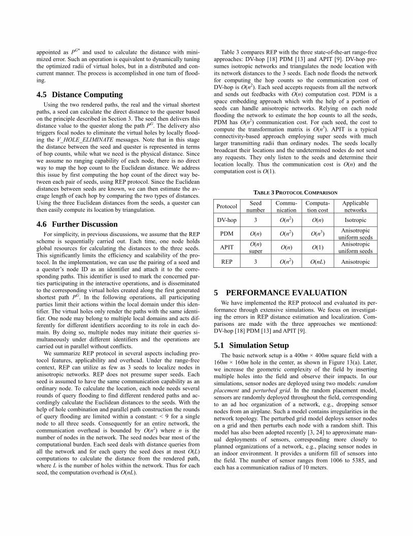
5.1 Simulation Setup The basic network setup is a 400m × 400m square field with a 160m × 160m hole in the center, as shown in Figure 13(a). Later, we increase the geometric complexity of the field by inserting multiple holes into the field and observe their impacts. In our simulations, sensor nodes are deployed using two models: random placement and perturbed grid. In the random placement model, sensors are randomly deployed throughout the field, corresponding to an ad hoc organization of a network, e.g., dropping sensor nodes from an airplane. Such a model contains irregularities in the network topology. The perturbed grid model deploys sensor nodes on a grid and then perturbs each node with a random shift. This model has also been adopted recently [3, 24] to approximate man-ual deployments of sensors, corresponding more closely to planned organizations of a network, e.g., placing sensor nodes in an indoor environment. It provides a uniform fill of sensors into the field. The number of sensor ranges from 1006 to 5385, and each has a communication radius of 10 meters.

(a) In perturbed grid deployment of 3024 nodes (average degree = 7.3), the real distance is 68.7 meters and the es-timated distance is 63.6 meters (7.4% error).

(b) In random deployment of 3027 nodes (average degree = 7.3), the real distance is 69.1 meters and the estimated distance is 77.2 meters (11.7% error).

(c) In perturbed grid deployment of 5376 nodes (average degree = 12.9), the real distance is 67.9 meters and the estimated distance is 64.2 meters (5.4% error).

(d) In random deployment of 5385 nodes (average degree = 12.9), the real distance is 68.9 meters and the estimated distance is 61.5 meters (10.7% error).

Figure 13: REP distance measurement under various settings.

Seed 1 (25, 85)

Seed 2 (40, 10)

Seed 3(80, 50)

1 2 3 4 5 6

0

10

20

30

40

50

Virtual hole radius (hops)

Erro

r rat

e (%

)

(a) (b)

Figure 14: REP distance estimation error V.S. virtual hole radius.

Figure 15: Localization performance under REP distance measurement.

(a) (b) (c)

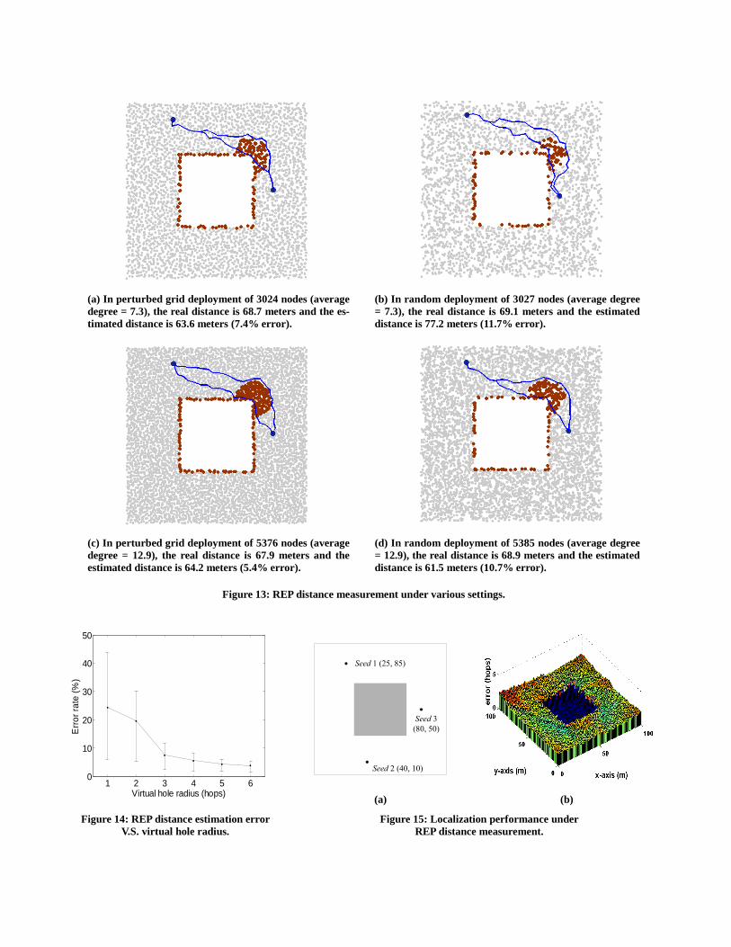
Figure 16: Network settings. (a) Basic setting, 5376 nodes (average degree = 12.9); (b) Two holes, 4697 nodes (average degree = 12.9); (c) Two holes (one concave), 5142 nodes (av-erage degree = 12.8).

TABLE 4 REP PERFORMANCE

Perturbed grid deployment Distance Localization

Number of de-ployed nodes (ave. degree)

Ave. distance estimation error (%)

Ave. local-ization error

(m)

Standard deviation (m)

n = 1986 (4.8) 11.4 25.5 9.7 n = 3024 (7.3) 5.6 15.2 6.5 n = 5376 (12.9) 3.5 10.4 4.3 n = 8407 (20.2) 3.2 10.2 3.5

Random deployment Distance Localization

Ave. distance estimation error (%)

Ave. local-ization error

(m)

Standard deviation (m)

n = 1979 (4.9)* N/A N/A N/A n = 3027 (7.3) 7.8 18.7 7.9 n = 5385 (12.9) 6.5 16.8 7.4 n = 8387 (20.1) 3.7 11.2 4.1

* The network seldom connects under this setting.

TABLE 5 PERFORMANCE COMPARISON

Distance Localization Network setting Ave. distance

estimation error (%)

Ave. localiza-tion error (m)

Standard deviation

(m) REP 3.5 10.4 4.3 Setting a

DV-hop 18.5 46.2 24.5 REP 4.4 11.5 6.2 Setting b

DV-hop 20.7 51.8 30.6 REP 4.1 10.6 4.9 Setting c

DV-hop 34.9 96.8 24.5

5.2 REP Performance We first focus on the distance measurement error of REP. Fig-ure 13 illustrates how REP works in a simple scenario. The two created paths, shortest and virtual shortest, are colored in blue. The boundary nodes and nodes within the virtual hole are marked with the color red. For simplicity, in the first simulation, we set the radius of the virtual holes as 4 hops, and later we show the impact of virtual hole radii.

We see that the error of REP under perturbed grid deployment is around 5-7%, which is better than that of REP under random deployment, around 11%. In all cases, the estimation error is less than 12%, and denser networks always have smaller errors. Actu-ally, in our simulations, the network hardly keeps connected with lower average degree. The performance shown in figure 13(b) provides the worst among all of the simulation results.

We have emphasized that the radii of virtual holes greatly affect the accuracy. We test this impact by varying the radius from 1 hop to 6 hops. Figure 14 plots the results when we conduct the simula-tion based on the network topology shown in figure 13(c). For each radius test, we randomly choose 50 sets of distance estimates (we choose node pairs whose connecting shortest path is at least 10 hops and involves boundary nodes) and record the errors. We observe that REP bears high errors on distance estimations when the virtual hole radii are small. The average estimation error is 24.3% for 1 hop radius and 19.5% for 2 hop radius. The deviation for the two cases is also high. As the radius is increased, the esti-mation error becomes limited and stabilized. Below 10% estima-tion error is preserved when the radius is larger than 3 hops. When the radius is set to 6, the worst case error is less than 5%, and the average is only 3.7%.

We then insert three seeds and locate ordinary nodes using REP. We use the same network setting as that shown in figure 13(c). The seeds have the same communication radius as ordinary nodes and are placed as shown in figure 15(a). Figure 15(b) plots the error map on the field. The localization error is estimated in terms of the average distance per hop (around 7.23 meters per hop in the simulation). Most of the errors are limited to below a 2 hops (be-low 15 meters). The nodes farther from the seeds often bear larger errors.

We vary network settings and estimate locations for every node using the REP protocol. Each experiment takes 10 runs and we report the average, as summarized in Table 4. Again, in both de-ployments, the distance estimation errors are smaller in denser networks, and consequently, localization errors and the corre-sponding standard deviation values are also lower.

5.3 Comparative Study We compare REP with DV-hop [18], PDM [13] and APIT [9] schemes. As previously mentioned, differing from REP, the three approaches are designed blind to the geometric features of net-works. Specifically, DV-hop targets isotropic networks and suffers large measurement errors in anisotropic networks with holes. PDM and APIT rely on the uniform deployment of a large number of seeds within the network to assist localization. REP outper-forms DV-hop PDM and APIT in the sense that REP achieves a much higher accuracy in anisotropic networks with the help of only 3 seeds. In this set of simulations, besides the basic settings shown in figure 16(a), we increase the geometric complexity of the network by inserting more holes, as shown in figure 16(b), and inserting a concave hole in the field, shown in figure 16(c). We assume (1) a perturbed grid deployment, (2) the density of nodes is kept consis-tent with the average degree around 12.9, and (3) only 3 seeds are deployed. Here PDM and APIT are not compared because the seeds are much fewer than they expect and thus lead to very poor perform-ance. We perform REP and DV-hop localization 10 runs for each setting and locate every node for each run. Table 5 shows the re-sults, where REP achieves much smaller errors in distance estima-tion and localization. The standard deviation of the localization

error in REP is also much smaller. Particularly, while REP achieves stable localization errors for the 3 settings, the perform-ance of DV-hop largely degrades as the network geometric com-plexity increases. In setting (c), DV-hop localization incurs 34.9% distance estimation error which means 96.8 meters in absolute distance. We increase the number of seeds so that we can also compare the performance with PDM and APIT. We examine the network settings of figure 16(a) - (c). The seeds are uniformly deployed in the field. We note that in the design of APIT, the transmitting range of seeds is assumed to be a factor ANR [9] of the transmit-ting range of a regular node. In our simulation, the factor ANR is assumed to be 10, which is the same as what APIT assumes.

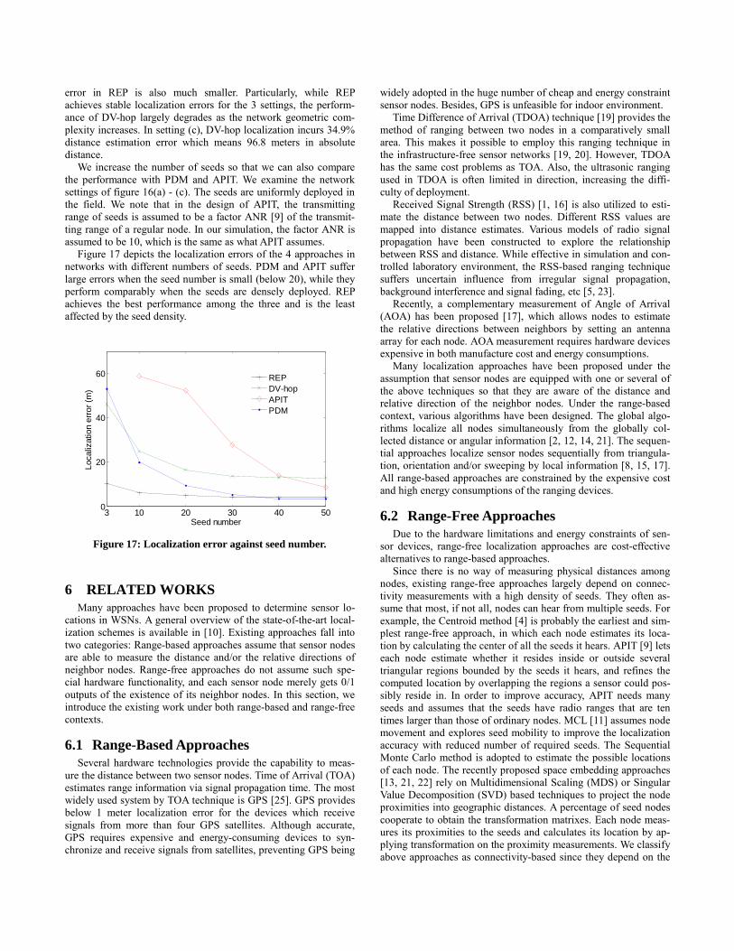
Figure 17 depicts the localization errors of the 4 approaches in networks with different numbers of seeds. PDM and APIT suffer large errors when the seed number is small (below 20), while they perform comparably when the seeds are densely deployed. REP achieves the best performance among the three and is the least affected by the seed density.

3 10 20 30 40 500

20

40

60

Seed number

Loca

lizat

ion

erro

r (m

)

REPDV-hopAPITPDM

Figure 17: Localization error against seed number.

6 RELATED WORKS

Many approaches have been proposed to determine sensor lo-cations in WSNs. A general overview of the state-of-the-art local-ization schemes is available in [10]. Existing approaches fall into two categories: Range-based approaches assume that sensor nodes are able to measure the distance and/or the relative directions of neighbor nodes. Range-free approaches do not assume such spe-cial hardware functionality, and each sensor node merely gets 0/1 outputs of the existence of its neighbor nodes. In this section, we introduce the existing work under both range-based and range-free contexts.

6.1 Range-Based Approaches Several hardware technologies provide the capability to meas-ure the distance between two sensor nodes. Time of Arrival (TOA) estimates range information via signal propagation time. The most widely used system by TOA technique is GPS [25]. GPS provides below 1 meter localization error for the devices which receive signals from more than four GPS satellites. Although accurate, GPS requires expensive and energy-consuming devices to syn-chronize and receive signals from satellites, preventing GPS being

widely adopted in the huge number of cheap and energy constraint sensor nodes. Besides, GPS is unfeasible for indoor environment. Time Difference of Arrival (TDOA) technique [19] provides the method of ranging between two nodes in a comparatively small area. This makes it possible to employ this ranging technique in the infrastructure-free sensor networks [19, 20]. However, TDOA has the same cost problems as TOA. Also, the ultrasonic ranging used in TDOA is often limited in direction, increasing the diffi-culty of deployment. Received Signal Strength (RSS) [1, 16] is also utilized to esti-mate the distance between two nodes. Different RSS values are mapped into distance estimates. Various models of radio signal propagation have been constructed to explore the relationship between RSS and distance. While effective in simulation and con-trolled laboratory environment, the RSS-based ranging technique suffers uncertain influence from irregular signal propagation, background interference and signal fading, etc [5, 23]. Recently, a complementary measurement of Angle of Arrival (AOA) has been proposed [17], which allows nodes to estimate the relative directions between neighbors by setting an antenna array for each node. AOA measurement requires hardware devices expensive in both manufacture cost and energy consumptions. Many localization approaches have been proposed under the assumption that sensor nodes are equipped with one or several of the above techniques so that they are aware of the distance and relative direction of the neighbor nodes. Under the range-based context, various algorithms have been designed. The global algo-rithms localize all nodes simultaneously from the globally col-lected distance or angular information [2, 12, 14, 21]. The sequen-tial approaches localize sensor nodes sequentially from triangula-tion, orientation and/or sweeping by local information [8, 15, 17]. All range-based approaches are constrained by the expensive cost and high energy consumptions of the ranging devices.

6.2 Range-Free Approaches Due to the hardware limitations and energy constraints of sen-sor devices, range-free localization approaches are cost-effective alternatives to range-based approaches. Since there is no way of measuring physical distances among nodes, existing range-free approaches largely depend on connec-tivity measurements with a high density of seeds. They often as-sume that most, if not all, nodes can hear from multiple seeds. For example, the Centroid method [4] is probably the earliest and sim-plest range-free approach, in which each node estimates its loca-tion by calculating the center of all the seeds it hears. APIT [9] lets each node estimate whether it resides inside or outside several triangular regions bounded by the seeds it hears, and refines the computed location by overlapping the regions a sensor could pos-sibly reside in. In order to improve accuracy, APIT needs many seeds and assumes that the seeds have radio ranges that are ten times larger than those of ordinary nodes. MCL [11] assumes node movement and explores seed mobility to improve the localization accuracy with reduced number of required seeds. The Sequential Monte Carlo method is adopted to estimate the possible locations of each node. The recently proposed space embedding approaches [13, 21, 22] rely on Multidimensional Scaling (MDS) or Singular Value Decomposition (SVD) based techniques to project the node proximities into geographic distances. A percentage of seed nodes cooperate to obtain the transformation matrixes. Each node meas-ures its proximities to the seeds and calculates its location by ap-plying transformation on the proximity measurements. We classify above approaches as connectivity-based since they depend on the

measure of connectivity between a node and the seeds. Their ma-jor limitation is that they all rely on a large number, generally proportional to the network size, of uniformly-distributed seeds in the network. DV-hop [18], employing a constant number of seeds, relies on the heuristic of proportionality between the distance and hop count in isotropic networks. The system estimates the aver-age-distance-per-hop from seed locations and the hop count among seeds. Each node measures the hop count to at least 3 seeds and translates these into distances. By triangulation, the location is then calculated. However, the DV-hop method yields high local-ization errors in anisotropic networks, where the existence of holes breaks the proportionality between the distance and hop count, and thus, leads to inaccurate location estimates.

7 CONCLUSIONS Locating sensors is necessary for many location-dependent applications that utilize wireless sensor networks. Due to high costs and critical assumptions, the range-based schemes are often impractical. The existing range-free schemes, however, suffer from poor accuracy and low scalability. Without the help of a large number of uniformly deployed super sensors, those schemes fail in anisotropic WSNs.

We propose the Rendered Path (REP) protocol, a range-free lo-calization scheme in anisotropic sensor networks. REP captures the geometric features of the network and disseminates such in-formation by rendering the shortest paths among nodes. By intro-ducing the virtual hole concept, REP constructs virtual shortest paths in order to estimate the distances between node pairs. The most important contributions of this work are that during localiza-tion, REP releases (1) necessity of ranging devices, (2) depend-ence on large numbers of uniformly deployed seed nodes, and (3) assumption of isotropic networks. Our analysis and simulations show the effectiveness and scalability of REP. We also compare the advantages of the REP against existing range-free approaches. We believe that our design will make the range-free localization schemes more practical for large-scale WSNs.

ACKNOWLEDGEMENT The authors would like to thank the anonymous reviewers for

their constructive feedback and valuable input. This work is sup-ported in part by the Hong Kong RGC grant HKUST6169/07E, the HKUST Digital Life Research Center Grant, the National Ba-sic Research Program of China (973 Program) under grant No. 2006CB303000, and NSFC Key Project grant No. 60533110.

REFERENCES [1] P. Bahl and V. N. Padmanabhan, “RADAR: An In-Building

RF-Based User Location and Tracking System,” in Proceed-ings of IEEE INFOCOM, 2000.

[2] P. Biswas and Y. Ye, “Semidefinite Programming for Ad Hoc Wireless Sensor Network Localization,” in Proceedings of IEEE/ACM IPSN, 2004.

[3] J. Bruck, J. Gao and A. A. Jiang, “MAP: Medial Axis Based Geometric Routing in Sensor Network,” in Proceedings of ACM MobiCom, 2005.

[4] N. Bulusu, J. Heidemann and D. Estrin, “GPS-less Low Cost Outdoor Localization For Very Small Devices,” IEEE Personal Communication Magazine, vol. 7(5), pp. 28 - 34, 2000.

[5] M. Carvalho and J. J. Garcia-Luna-Aceves, “A Scalable Model for Channel Access Protocols in Multihop Ad Hoc Networks,” in Proceedings of ACM MobiCom, 2004.

[6] S. P. Fekete, A. Kroller, D. Pfister, S. Fischer and C. Busch-mann, “Neighbor-based Topology Recognition in Sensor Net-works,” in Proceedings of ALGOSENSORS, 2004.

[7] S. Funke, “Topological Hole Detection in Wireless Sensor Networks and its Applications,” in Proceedings of Joint Work-shop on Foundations of Mobile Computing, 2005.

[8] D. Goldenberg, P. bihler, M. Gao, J. Fang, B. Anderson, et al., “Localization in Sparse Networks using Sweeps,” in Proceed-ings of ACM MobiCom, 2006.

[9] T. He, C. Huang, B. M. Blum, J. A. Stankovic and T. F. Abdel-zaher, “Range-Free Localization Schemes in Large Scale Sen-sor Networks,” in Proceedings of ACM MobiCom, 2003.

[10] J. Hightower and G. Borriello, “Location Systems for Ubiqui-tous Computing,” IEEE Computer, vol. 34, pp. 57 - 66, 2001.

[11] L. Hu and D. Evans, “Localization for Mobile Sensor Net-works,” in Proceedings of ACM MobiCom, 2004.

[12] X. Ji and H. Zha, “Sensor Positioning in Wireless Ad-hoc Sen-sor Networks with Multidimensional Scaling,” in Proceedings of IEEE INFOCOM, 2004.

[13] H. Lim and J. C. Hou, “Localization for Anisotropic Sensor Networks,” in Proceedings of IEEE INFOCOM, 2005.

[14] H. Lim, L. Kung, J. Hou and H. Luo, “Zero-Configuration, Robust Indoor Localization: Theory and Experimentation,” in Proceedings of IEEE INFOCOM, 2006.

[15] D. Moore, J. Leonard, D. Rus and S. Teller, “Robust Distrib-uted Network Localization with Noisy Range Measurements,” in Proceedings of ACM SenSys, 2004.

[16] L. M. Ni, Y. Liu, Y. C. Lau and A. Patil, “LANDMARC: In-door Location Sensing Using Active RFID,” in Proceedings of IEEE PerCom, 2003.

[17] D. Niculescu and B. Nath, “Ad Hoc Positioning System (APS) using AOA,” in Proceedings of IEEE INFOCOM, 2003.

[18] D. Niculescu and B. Nath, “DV Based Positioning in Ad Hoc Networks,” Journal of Telecommunication Systems, 2003.

[19] A. Savvides, C. Han and M. B. Srivastava, “Dynamic Fine-Grained Localization in Ad-Hoc Networks of Sensors,” in Proceedings of ACM MobiCom, 2001.

[20] A. Savvides, H. Park and M. Srivastava, “The Bits and Flops of the N-Hop Multilateration Primitive for Node Localization Problems,” in Proceedings of ACM WSNA, 2002.

[21] Y. Shang and W. Ruml, “Improved MDS-Based Localization,” in Proceedings of IEEE INFOCOM, 2004.

[22] Y. Shang, W. Ruml, Y. Zhang and M. P. J. Fromherz, “Local-ization from mere connectivity,” in Proceedings of ACM Mo-biHoc, 2003.

[23] S. Vedantam, U. Mitra and A. Sabharwal, “Sensing the Channel Sensor Networks with Shared Sensing and Communications,” in Proceedings of IEEE/ACM IPSN, 2006.

[24] Y. Wang, J. Gao and J. S. B. Mitchell, “Boundary Recognition in Sensor Networks by Topological Methods,” in Proceedings of ACM MobiCom, 2006.

[25] B. H. Wellenhoff, H. Lichtenegger and J. Collins, Global Posi-tioning System: Theory and Practice: Springer Verlag, 1997.