Embed Size (px)
Citation preview
UNIVERSIDADE FEDERAL DE SANTA CATARINA
PROGRAMA DE PÓS - GRADUAÇÃO EM ENGENHARIA DE
AUTOMAÇÃO E SISTEMAS
Renan Augusto Starke
DESIGN AND EVALUATION OF A VLIW
PROCESSOR FOR REAL-TIME SYSTEMS
Florianópolis
2016

Renan Augusto Starke
DESIGN AND EVALUATION OF A VLIW PROCESSOR FOR
REAL-TIME SYSTEMS
A Thesis submitted to the Automa-tion and Systems Engineering Post-graduate Program in partial fulfillmentof the requirements for the degree ofDoctor of Philosophy in Automationand Systems Engineering.Supervisor: Rômulo Silva de Oliveira
Florianópolis2016
Ficha de identificação da obra elaborada pelo autor, através do Programa de Geração Automática da Biblioteca Universitária da UFSC.
Starke, Renan Augusto Design and Evaluation of a VLIW Processor for Real-TimeSystems / Renan Augusto Starke ; orientador, Rômulo Silvade Oliveira - Florianópolis, SC, 2016. 204 p.
Tese (doutorado) - Universidade Federal de SantaCatarina, Centro Tecnológico. Programa de Pós-Graduação emEngenharia de Automação e Sistemas.
Inclui referências
1. Engenharia de Automação e Sistemas. 2. Real timesystems. 3. Very Long Instruction Word (VLIW) processor.4. Worst-Case Execution Time (WCET) Analysis. I. Oliveira,Rômulo Silva de. II. Universidade Federal de SantaCatarina. Programa de Pós-Graduação em Engenharia deAutomação e Sistemas. III. Título.
DESIGN AND EVALUATION OF A VLIW PROCESSOR FORREAL-TIME SYSTEMS
Renan Augusto Starke
This Thesis is hereby approved and recommended for acceptance in partialfulfillment of the requirements for the degree of “Doctor of philosophy in
Automation and Systems Engineering.”
June 6th, 2016.
Prof. Rômulo Silva de Oliveira, Dr.Supervisor
Prof. Daniel Coutinho, Dr.Coordinator of the Automation and Systems
Engineering Postgraduate Program
Examining Committee:
Prof. Rômulo Silva de Oliveira, Dr. – UFSCChair
Prof. Anderson Luiz Fernandes Perez, Dr. – UFSC
Prof. Joni da Silva Fraga, Dr. – UFSC
Prof. Rafael Rodrigues Obelheiro, Dr. – UDESC
Prof. Rodolfo Jardim de Azevedo, Dr. – UNICAMP
Prof. Werner Kraus Junior, Dr. – UFSC
Explanations exist: they have existed for all times, forthere is always an easy solution to every problem – neat,plausible and wrong.– H.L. Mencken, “The Divine Afflatus”, in the New YorkEvening Mail, November 16, 1917


ACKNOWLEDGEMENTS
I thank to professor Rômulo Silva de Oliveira for his dedica-tion, encouragement, patience and the great suggestions when the wayseemed unclear.
I thank my family for their trust and support during the course.In particular I thank my parents allowing access to high quality edu-cation. A special thank to my future wife Allessa Mariá Maiochi whowaited and supported me for these years.
I also thank to laboratory colleagues for friendship, help in cor-rections, sharing and improvement of ideas. A special thank to myfriend Andreu Carminati who helped to make this work possible withthe compiler back-end implementation, ideas and tips.
Finally thanks to CAPES for the financial support that enabledthis work.

ABSTRACT
Nowadays, many real-time applications are very complex and as the com-plexity and the requirements of those applications become more demand-ing, more hardware processing capacity is necessary. The correct func-tioning of real-time systems depends not only on the logically correct re-sponse, but also on the time when it is produced. General purpose proces-sor design fails to deliver analyzability due to their non-deterministic be-havior caused by the use of cache memories, dynamic branch prediction,speculative execution and out-of-order pipelines. In this thesis, we designand evaluate the performance of VLIW (Very Long Instruction Word) ar-chitectures for real-time systems with an in-order pipeline consideringWCET (Worst-case Execution Time) performance. Techniques on ob-taining the WCET of VLIW machines are also considered and we makea quantification on how important are hardware techniques such as staticbranch prediction, predication, pipeline speed of complex operations suchas memory access and multiplication for high-performance real-time sys-tems. The memory hierarchy is out of scope of this thesis and we useda classic deterministic structure formed by a direct mapped instructioncache and a data scratchpad memory. A VLIW prototype was imple-mented in VHDL from scratch considering the HP VLIW ST231 ISA.We also show some compiler insights and we use a representative subsetof the Mälardalen’s WCET benchmarks for validation and performancequantification. Supporting our objective to investigate and evaluate hard-ware features which reconcile determinism and performance, we madethe following contributions: design space investigation and evaluation re-garding VLIW processors, complete WCET analysis for the proposed de-sign, complete VHDL design and timing characterization, detailed brancharchitecture, low-overhead full-predication system for VLIW processors.
Keywords: Real time systems, Very Long Instruction Word (VLIW) pro-cessor, Worst-Case Execution Time (WCET) Analysis.

RESUMO EXPANDIDO
CONSIDERAÇÕES SOBRE PROJETO DE PROCESSADORESVLIW PARA SISTEMAS DE TEMPO REAL
Palavras-chave: Sistemas de tempo real, processadores VLIW (Very-Long Instruction Word), análise de pior tempo de computação (WCET– Worst-case Execution Time)
Introdução
Atualmente, aplicações de tempo estão tornando-se cada vez maiscomplexas e, conforme os requisitos destes sistemas aumentam, maior é ademanda por capacidade de processamento. Contudo, o correto funciona-mento destas aplicações não está em função somente da correta respostalógica, mas também no tempo que ela é produzida.
Nos últimos anos, houve uma quantidade significativa de pesquisasvoltadas a arquiteturas de processadores temporalmente previsíveis como intuito de utilizá-los em sistemas de tempo real. Como o principal ob-jetivo de projeto de processadores de propósito geral tem-se mantido namelhora do desempenho de caso médio, a utilização destes em sistemas detempo real tornou-se consideravelmente complexa devido à necessidadede análises para obtenção de parâmetros temporais.
Sistemas de tempo real são geralmente modelados por um conjuntode tarefas onde cada uma possui seu pior tempo de execução (WCET –Worst-case Execution Time), período e prazo (deadline) e estes parâme-tros são utilizados em testes de escalonabilidade formais. Em conjuntocom um algoritmo de escalonamento de tarefas, é formado um problemade escalonabilidade onde o objetivo é verificar se todas as tarefas cum-prem seus deadlines: o tempo de resposta de uma tarefa deve sempreser menor ou igual ao seu respectivo deadline. Obter o pior tempo decomputação tem se mostrado complexo e dependente de parâmetros re-lacionados ao hardware como arquitetura do processador e da memória.Obter o WCET eficientemente e com precisão é necessário tanto para omais simples quanto ao mais complexo teste de escalonabilidade.
As principais abordagens para obter o WCET são medições, análisesestáticas e análises híbridas. A prática mais comum na indústria é o usode medições executando o sistema no hardware alvo. Nas análises estáti-cas, não há execução mas a estimação do WCET é realizada utilizando-sede um modelo matemático constituído pelo o binário da tarefa e caracte-rísticas da plataforma alvo. No caso das análises híbridas, são combina-das análises estáticas com medições. Independentemente da abordagem,ferramentas de análise WCET fornecem uma estimativa do tempo de exe-cução de um código que deverá ser igual ou maior que WCET real. Apli-cações complexas são difíceis de analisar por qualquer abordagem (GUS-TAFSSON, 2008). Análises estáticas podem gerar problemas complexosnão escaláveis geralmente relacionados ao hardawre, enquanto mediçõesnecessitam de casos de uso que não necessariamente produzem o WCETde uma aplicação. Para amenizar o problema relacionado a estimação doWCET, tem-se mostrado interesse em arquiteturas projetadas especifica-mente para sistemas de tempo real, como os trabalhos de (SCHOEBERLet al., 2011), (LIU et al., 2012) e (SCHOEBERL et al., 2015)
Nesta tese, investiga-se uma arquitetura de processador VLIW –Very-Long Instruction Word especificamente projetada para sistemas detempo real considerando sua análise do pior tempo de computação (WCET– Worst-case Execution Time). Técnicas para obtenção do WCET paramáquinas VLIW são consideradas e quantifica-se a importância de técni-cas de hardware como previsor de fluxo estático, predicação, bem comovelocidade do processador para instruções complexas como acesso a me-mória e multiplicação. A arquitetura de memória não faz parte do escopodeste trabalho e para tal utilizamos uma estrutura determinista formadapor uma memória cache com mapeamento direto para instruções e umamemória de rascunho (scratchpad) para dados. Nós também considera-mos a implementação em VHDL do protótipo para inferir suas caracterís-ticas temporais mantendo compatibilidade com o conjunto de instruções(ISA) HP VLIW ST231. Em termos de avaliação, foi utilizado um con-junto representativo de código exemplos da Universidade de Mälardalenque é amplamente utilizado em avaliações de sistemas de tempo-real.
Objetivos
O objetivo desta tese é investigar características de arquitetura deprocessadores que levam a um projeto determinista mas também que con-sideram o desempenho de pior caso (redução do WCET). A tese a serdemonstrada é que é possível utilizar elementos de hardware que aumen-tam o desempenho mas que são previsíveis o suficiente para garantir umaanálise estática eficiente e precisa. Para demonstrar previsibilidade, é in-teressante demonstrar as técnicas de análise envolvidas na obtenção deWCET de tarefas. Portanto, a construção de uma ferramenta de WCETassim como os aspectos envolvidos na modelagem do hardware tambémsão assuntos cobertos neste trabalho.
Entre os elementos arquiteturais considerados, têm-se:
∙ Pipeline:
Pipeline é uma técnica que permite que operações complexas sejamorganizadas em outras mais simples com o objetivo de aumentar de-sempenho. No caso de processadores deterministas, pipelines sãonecessários mas as instruções devem ser executadas em ordem. Pi-pelines com execução fora de ordem permitem um alto desempenhode caso médio mas prejudicam a análise de WCET devido a anoma-lias temporais (LUNDQVIST; STENSTROM, 1999).
∙ Paralelismo entre instruções:
Nos processadores modernos, o termo superescalar é utilizado quandomais de uma instrução é executada em cada estágio de pipeline. Esteprojeto supera a limitação de desempenho (throughput) de apenasuma instrução executada por ciclo de máquina. No caso de proces-sadores para sistemas de tempo-real, a execução de múltiplas ins-truções por estágio de pipeline também pode ser utilizado utilizandoum projeto Very Long Instruction Word (VLIW) (FISHER; FARA-BOSHI; YOUNG, 2005). Máquinas VLIW são mais adequadas parasistemas de tempo real pois o escalonamento de instruções é deter-minado pelo compilador e não em tempo de execução. Isso simpli-fica a análise estática, pois escalonamento dinâmico de instruções
não precisa ser modelado.
∙ Primeiro nível do sub-sistema de memória:
O sub-sistema de memória é um assunto relevante em vários traba-lhos (REINEKE et al., 2011). Há diversas abordagens e algumasdelas requerem modificações complexas no compilador ou no hard-ware (SCHOEBERL et al., 2011). Neste trabalho, nós tratamos daprevisibilidade do sub-sistema de memória utilizando uma memóriacache de instruções com mapeamento direto bem como uma memó-ria de rascunho (scratchpad) para dados. Memórias de rascunho sãosimilares às caches mas seu conteúdo é gerenciado explicitamentepelo software.
∙ Previsão de fluxo:
Modificações no controle de fluxo de um programa são realizadaspor instruções especiais chamadas branches. Elas são utilizadas paraestruturas com condicionamentos (if ), laços (for e while) e geral-mente degradam o desempenho do pipeline devido a ciclos de para-das (stalls). Uma maneira de reduzir esta limitação é o uso de previ-sores de fluxo. Há os previsores dinâmicos e os estáticos. Os dinâ-micos prejudicam a previsibilidade enquanto os estáticos possuemcaracterísticas interessantes para sistemas de tempo real (BURGUI-ERE; ROCHANGE; SAINRAT, 2005). Nós consideraremos os pre-visores estáticos, demonstrando sua importância em termos de de-sempenho bem como a metodologia para considerá-los na análiseWCET.
∙ Predicação:
Predicação é uma técnica na qual instruções são condicionalmenteexecutadas baseando-se em um registrador Booleano. É diferentedos branches pois não há qualquer modificação no fluxo do pro-grama para ignorar instruções. Há dois tipos de predicação: com-pleta e parcial. Predicação completa permite que instruções sejamexecutadas ou ignoradas diretamente conforme o valor de um re-gistrador Booleano (esta predicação é comumente empregada nosprocessadores ARM). No caso da predicação parcial, instruções não
são ignoradas mas dois valores podem ser selecionados utilizandoum tipo especial de instrução (select). Predicação é uma técnica im-portante para reduzir caminhos em um programa induzindo o para-digma da programação de caminho único (Single-path programmingparadigm) (PUSCHNER, 2005). Nós suportamos ambos os tipos depredicação e a versão completa é reestruturada para reduzir o im-pacto no hardware.
∙ Instruções aritméticas complexas:
Há várias instruções aritméticas complexas como divisão e multipli-cação que diminuem o desempenho do processador. Frequentementeestas instruções são suportadas apenas por software, principalmentea divisão. Neste trabalho, tanto divisão quanto multiplicação porhardware são implementadas para que tenham previsibilidade inde-pendentemente de seus parâmetros de entrada.
Contribuições
Dentre as contribuições deste trabalho, nós podemos citar: inves-tigação sobre o espaço de projeto, avaliação de desempenho através deconjunto representativo de códigos exemplos, detalhamento completo daanálise estática, implementação VHDL, caracterização temporal de cadacomponente de hardware, detalhamento da arquitetura de controle defluxo e um sistema de predicação completo de baixo impacto para pro-cessadores VLIW.
Realizou-se uma avaliação extensiva das técnicas apontadas acimaconsiderando os benefícios em termos de desempenho de pior caso. Notou-se que uma avaliação tão ampla nunca havia sido considerada nos traba-lhos relacionados pois nestes são focados objetivos específicos como sub-sistema de memória, multi-threading ou multi-core. Nossa avaliação podeguiar novas linhas de pesquisas relacionadas com sistemas de tempo real.
Foram também abordadas todas as análises necessárias para estimaro WCET de programas compilados para o processador considerado nestetrabalho, incluindo cache, modelagem do pipeline e busca do pior cami-
nho do programa. Uma descrição completa de uma análise WCET paraprocessadores VLIW também não foi abordada nos trabalhos relaciona-dos.
Todos os detalhes da arquitetura de controle de fluxo são descri-tos, incluindo a metodologia para modelagem durante a análise WCET.Também ampliamos o ISA para suportar previsão de desvio estático, bemcomo os benefícios de usar ou não esta tecnologia em sistemas de temporeal.
Quanto ao sistema de predicação completo, foi proposto um sistemaque adiciona baixa sobrecarga nos caminhos de dados de hardware e nasua lógica de atalhos (forwarding logic). O sistema proposto diminui ouso de instruções de controle de fluxo, bem como permite a utilizaçaode técnicas de desenrolamento de laços (loop unrolling). No entanto, apredicação sozinha não é suficiente para aumentar o desempenho e pre-visibilidade e seu uso pode aumentar o tempo de execução (WCET). De-vido a isso, propõe-se o uso de uma abordagem híbrida com suporte dehardware para predicação e previsão estática de fluxo. Isto leva a umaredução significativa do pior tempo de computação e permite otimizaçõesdurante a compilação que pode selecionar a técnica apropriada para cadaestrutura.
Conclusão
Neste trabalho considerou-se elementos arquiteturais de processa-dores que beneficiam a análise estática mas também contribuem para oaumento do desempenho, principalmente para o pior caso de execução.
Como sistemas modernos impõem maiores requisitos funcionais,processadores de maior desempenho são necessários. Portanto, é neces-sário analisar os pontos fortes das técnicas de hardware usadas em pro-cessadores modernos, por exemplo paralelismo temporal e espacial naexecução de instruções, previsão de desvios e predição, e para adaptá-lospara aplicações em tempo real. Algumas destas técnicas exigem modifica-ções, devido à alta complexidade do hardware, enquanto outros precisamde um comportamento temporal bem definido. Para atingir esses objeti-
vos, foram propostas novas abordagens, a fim de melhorar a eficiência ea escalabilidade da análise temporal, especialmente a análise de tempo deexecução do pior caso. Mostrou-se que o projeto de processadores deveaumentar o nível de importância do determinismo.
Foi possível verificar através dos testes de desempenho que as técni-cas abordadas aumentaram o desempenho em todos os programas consi-derados. Além disso, mostrou-se detalhadamente as técnicas necessáriaspara realizar análise estática obtendo assim o WCET para todos progra-mas testados.
A implementação VHDL do processador mostrou-se desafiadoramas contribuiu significativamente para a caracterização temporal de cadaelemento de hardware.

LIST OF FIGURES
Figure 1 – The worst-case execution time problem . . . . . . . . . 32Figure 2 – Example of timing anomaly . . . . . . . . . . . . . . . 34Figure 3 – Generic 5-stage pipeline representation. . . . . . . . . . 49Figure 4 – Generic 5-stage pipeline with forward paths. . . . . . . 51Figure 5 – Diversified pipeline example. . . . . . . . . . . . . . . 53Figure 6 – Example of a dynamic pipeline. . . . . . . . . . . . . . 54Figure 7 – Example of a two-bit branch predictor (SHEN et al.,
2005). . . . . . . . . . . . . . . . . . . . . . . . . . . 57Figure 8 – Instruction bundle decoding example. . . . . . . . . . . 87Figure 9 – VLIW processor overview. . . . . . . . . . . . . . . . 90Figure 10 – Detail of execution units stages. . . . . . . . . . . . . . 92Figure 11 – Pipeline behavior of a “not taken” branch. . . . . . . . 98Figure 12 – Pipeline behavior of a “taken” directed branch. . . . . . 100Figure 13 – Pipeline behavior of a “taken” branch without direction
change or other direct control flow operations. . . . . . 100Figure 14 – Pipeline behavior of a mispredicted direction. . . . . . 101Figure 15 – Memory unit logic diagram. . . . . . . . . . . . . . . . 104Figure 16 – VLIW processor overview (reproduced from Figure 9). 112Figure 17 – Cache VHDL component. . . . . . . . . . . . . . . . . 112Figure 18 – Cache states and behavior. . . . . . . . . . . . . . . . . 113Figure 19 – ROM controller behavior. . . . . . . . . . . . . . . . . 114Figure 20 – Instruction bundle decoder VHDL component. . . . . . 115Figure 21 – Cache buffer component. . . . . . . . . . . . . . . . . 116Figure 22 – Front-end control behavior. . . . . . . . . . . . . . . . 118Figure 23 – Wave form of the pipeline front-end. . . . . . . . . . . 119Figure 24 – Control flow unit component. . . . . . . . . . . . . . . 121Figure 25 – Logic diagram for one read port. . . . . . . . . . . . . 124Figure 26 – Pipeline inter-stage responsible for the predication logic.126Figure 27 – Pipeline behavior of interlock RAW dependency. . . . . 128Figure 28 – Arithmetic and logic unit diagram. . . . . . . . . . . . 130Figure 29 – Forward logic multiplexers for one ALU. . . . . . . . . 130Figure 30 – Memory unit states and behavior . . . . . . . . . . . . 132
Figure 31 – Memory effective address calculation with forward. . . 133Figure 32 – Multiplication and division unit components per slot. . 135Figure 33 – Multiplication and division unit states and behavior . . 136Figure 34 – Data-flow between the compiler and WCET/linker . . . 141Figure 35 – Control flow graph example. . . . . . . . . . . . . . . 143Figure 36 – Cache abstract reachable state example . . . . . . . . . 148Figure 37 – CONFLICT classification example. . . . . . . . . . . . 151Figure 38 – Example of timing composition of two successive (lin-
ear addresses) basic blocks . . . . . . . . . . . . . . . 154Figure 39 – Example of a C program and its control-flow graph. . . 157Figure 40 – Multigraph of the example . . . . . . . . . . . . . . . . 161Figure 41 – WCET final result of example of Figure 39 . . . . . . . 162Figure 42 – WCET reduction between single-issue and four-issue. . 170Figure 43 – WCET reduction on using branch prediction. Under-
lined ones have null reduction. . . . . . . . . . . . . . 172Figure 44 – WCET reduction with dual-ported scratchpad. Under-
lined ones have null reduction. . . . . . . . . . . . . . 173Figure 45 – WCET reduction on using predication. . . . . . . . . . 174Figure 46 – Total WCET reduction. . . . . . . . . . . . . . . . . . 175
LIST OF TABLES
Table 1 – Arithmetic instructions specification. . . . . . . . . . . . 46Table 2 – Memory instructions specification. . . . . . . . . . . . . 47Table 3 – Control flow instructions specifications. . . . . . . . . . 47Table 4 – Maximum necessary stall cycles for dependency reso-
lution. . . . . . . . . . . . . . . . . . . . . . . . . . . . 50Table 5 – Maximum necessary stall cycles for dependency reso-
lution with forward paths. . . . . . . . . . . . . . . . . 51Table 6 – Basic differences between VLIW and Superscalar designs 55Table 7 – Comparison between branch code, full and partial pred-
ication (HP ST200 ISA – Apendix A). . . . . . . . . . . 59Table 8 – Comparison of techniques for general-purpose and real-
time processors . . . . . . . . . . . . . . . . . . . . . . 65Table 9 – Summary of related project objectives . . . . . . . . . . 77Table 10 – Operation encoding. . . . . . . . . . . . . . . . . . . . 88Table 11 – Example of simple true mode predication system. . . . . 95Table 12 – Example of complete mode predication system. . . . . . 96Table 13 – Example of nested if-then-else with full and partial pred-
ication systems. . . . . . . . . . . . . . . . . . . . . . . 97Table 14 – Example of data dependency between operations. . . . . 106Table 15 – Operation packing considering anti-dependencies, and
ignoring them. . . . . . . . . . . . . . . . . . . . . . . 107Table 16 – Instruction alignment in basic blocks. . . . . . . . . . . 108Table 17 – Pipeline features comparison . . . . . . . . . . . . . . . 110Table 18 – Cache address fields . . . . . . . . . . . . . . . . . . . 113Table 19 – Example of interlock cases. . . . . . . . . . . . . . . . . 127Table 20 – FPGA resources usage (Cyclone IV GX – EP4CGX15
0DF31C7). Resource usage reported by Quartus II 64-bit V 15.0.0 Build 145 WEB Edition. . . . . . . . . . . 138
Table 21 – Processor instruction timing . . . . . . . . . . . . . . . 139Table 22 – Additional time for multicycle instruction timing . . . . 153Table 23 – Modeling factor for each type of transition flow . . . . . 155Table 24 – Objective function modeling using Language MathProg. 156
Table 25 – Control-flow conservation restrictions using languageMathProg. . . . . . . . . . . . . . . . . . . . . . . . . . 158
Table 26 – Loop restrictions using language MathProg. . . . . . . . 159Table 27 – Conservation restrictions using language MathProg. . . . 159Table 28 – Cache restrictions using language MathProg. . . . . . . 162Table 29 – Mälardalen WCET benchmarks (GUSTAFSSON et al.,
2010) . . . . . . . . . . . . . . . . . . . . . . . . . . . 166Table 30 – Execution and worst-case performance comparing VEX
and our prototype and WCET absolute values. WCETand Exec. time in cycles. IPC is Instructions per cycle . 168
Table 31 – List of operation operands . . . . . . . . . . . . . . . . 197Table 32 – List of supported operations . . . . . . . . . . . . . . . 202
CONTENTS
1 INTRODUCTION . . . . . . . . . . . . . . . . . . 311.1 Basic concepts and motivation . . . . . . . . . . . . 321.1.1 Timing anomalies . . . . . . . . . . . . . . . . . . . 331.1.2 Timing predictability . . . . . . . . . . . . . . . . . 341.1.3 Timing composabilty . . . . . . . . . . . . . . . . . 361.2 Thesis objective . . . . . . . . . . . . . . . . . . . . 371.3 Contributions . . . . . . . . . . . . . . . . . . . . . 401.4 Text organization . . . . . . . . . . . . . . . . . . . 41
2 PROCESSORS AND PREDICTABILITY CONSID-ERATIONS . . . . . . . . . . . . . . . . . . . . . . 43
2.1 Pipeline principles . . . . . . . . . . . . . . . . . . 442.1.1 Minimizing pipeline stalls . . . . . . . . . . . . . . 472.2 Multiple instruction fetching . . . . . . . . . . . . . 522.2.1 Out-of-order execution . . . . . . . . . . . . . . . . 522.2.2 In-order execution . . . . . . . . . . . . . . . . . . 542.3 Branch prediction . . . . . . . . . . . . . . . . . . . 562.4 Predication . . . . . . . . . . . . . . . . . . . . . . 582.5 Cache memories . . . . . . . . . . . . . . . . . . . . 602.6 Scratchpad Memory . . . . . . . . . . . . . . . . . 612.7 Chip Multithreading . . . . . . . . . . . . . . . . . 622.8 Chip Multiprocessing . . . . . . . . . . . . . . . . . 632.9 Summary . . . . . . . . . . . . . . . . . . . . . . . 64
3 RELATED WORK . . . . . . . . . . . . . . . . . . 673.1 The Komodo approach . . . . . . . . . . . . . . . . 673.1.1 Real-time jamuth . . . . . . . . . . . . . . . . . . . 683.2 The JOP Java processor . . . . . . . . . . . . . . . 693.3 The MCGREP processor . . . . . . . . . . . . . . . 703.4 The PRET architecture . . . . . . . . . . . . . . . . 713.5 The Patmos approach . . . . . . . . . . . . . . . . . 723.6 The CarCore processor . . . . . . . . . . . . . . . . 73
3.7 Multicore solutions . . . . . . . . . . . . . . . . . . 743.7.1 The Merasa project . . . . . . . . . . . . . . . . . . 743.7.2 The T-CREST project . . . . . . . . . . . . . . . . 753.8 Summary . . . . . . . . . . . . . . . . . . . . . . . 75
4 THESIS RATIONALE AND DESIGN DECISIONS 794.1 Target systems and requirements . . . . . . . . . . 804.2 Thesis Objective . . . . . . . . . . . . . . . . . . . . 814.3 Architecture . . . . . . . . . . . . . . . . . . . . . . 824.4 Design decisions . . . . . . . . . . . . . . . . . . . . 854.4.1 Instruction set and encoding . . . . . . . . . . . . . 854.4.1.1 Instruction bundle encoding . . . . . . . . . . . . . . . 85
4.4.1.2 Operation encoding . . . . . . . . . . . . . . . . . . . 88
4.4.2 Processor pipeline . . . . . . . . . . . . . . . . . . . 894.4.3 Predication . . . . . . . . . . . . . . . . . . . . . . 934.4.4 Branch prediction . . . . . . . . . . . . . . . . . . . 954.4.5 First level of the memory subsystem . . . . . . . . . 1014.4.5.1 Instruction cache . . . . . . . . . . . . . . . . . . . . . 102
4.4.5.2 Data memory interface . . . . . . . . . . . . . . . . . . 103
4.4.6 Compiler support . . . . . . . . . . . . . . . . . . . 1054.5 Summary . . . . . . . . . . . . . . . . . . . . . . . 109
5 VHDL IMPLEMENTATION AND TIMING CHAR-ACTERISTICS . . . . . . . . . . . . . . . . . . . . 111
5.1 Instruction cache . . . . . . . . . . . . . . . . . . . 1115.2 Pipeline front-end . . . . . . . . . . . . . . . . . . . 1155.3 The control-flow system . . . . . . . . . . . . . . . 1205.4 Register files . . . . . . . . . . . . . . . . . . . . . . 1225.5 Predication support . . . . . . . . . . . . . . . . . . 1255.6 Pipeline interlock . . . . . . . . . . . . . . . . . . . 1275.7 Arithmetic and Logic units . . . . . . . . . . . . . . 1295.8 Data memory interface . . . . . . . . . . . . . . . . 1325.9 Multiplication and division unit . . . . . . . . . . . 1335.10 Timing characteristics and FPGA resource utilization137
5.11 Summary . . . . . . . . . . . . . . . . . . . . . . . 137
6 WORST-CASE EXECUTION TIME ANALYSIS . 1416.1 Basic concepts . . . . . . . . . . . . . . . . . . . . . 1426.2 Instruction cache analysis . . . . . . . . . . . . . . 1456.2.1 Reachable and effective abstract state . . . . . . . . 1466.2.2 Cache accesses classification . . . . . . . . . . . . . 1496.3 Pipeline modeling . . . . . . . . . . . . . . . . . . . 1506.4 Worst-case path search . . . . . . . . . . . . . . . . 1546.4.1 ILP Constraints . . . . . . . . . . . . . . . . . . . . 1576.5 Summary . . . . . . . . . . . . . . . . . . . . . . . 163
7 EVALUATION . . . . . . . . . . . . . . . . . . . . 1657.1 Impact of the compiler on the performance . . . . . 1677.2 Use of processors with wider fetch . . . . . . . . . . 1697.3 Use of “taken”/“not taken” static branch prediction 1717.4 Reducing execution stage overhead . . . . . . . . . 1727.5 Predication . . . . . . . . . . . . . . . . . . . . . . 1737.6 Overall reduction and impact on WCET calculation 1747.7 Contributions to the state of the art . . . . . . . . . 176
8 FINAL REMARKS . . . . . . . . . . . . . . . . . . 1798.1 Publications . . . . . . . . . . . . . . . . . . . . . . 1838.2 Suggestions of future work . . . . . . . . . . . . . . 184
BIBLIOGRAPHY . . . . . . . . . . . . . . . . . . . 187
APPENDIX 195
APPENDIX A – LIST OF SUPPORTED OPERA-TIONS . . . . . . . . . . . . . . . 197

27
LIST OF ABBREVIATIONS AND ACRONYMS
ALU Arithmetic Logic Unit
BCET Best-Case Execution Time
CISC Complex Instruction Set Computing
FPGA Field-Programmable Gate Array
FSM Finite State Machine
ISA Instruction Set Architecture
LLVM Low Level Virtual Machine compiler infrastructure
LVT Live Value Table
NOP No Operation
RAM Random Access Memory
RISC Reduced Instruction Set Computing
ROM Read-Only Memory
SRAM Static Random Access Memory
VEX VLIW Example
VHDL VHSIC Hardware Description Language
VHSIC Very High Speed Integrated Circuit
VLIW Very Long Instruction Word
WCET Worst-Case Execution Time

29
LIST OF SYMBOLS
CFG Control-Flow Graph
d j_i Edge from node j to i
δ Transition-flow modeling factor
E Edge set of a graph
EMBi(c) Effective Memory Block set of a basic block i andcache line c
G Graph
nc Total number of cache misses inside a basic block
nm Total number of high latency memory access insidea basic block
RMBi(c) Reaching Memory Block set of a basic block i andcache line c
tbb Basic-block time
tc Cache-miss time
ti_ j Time of basic block i when executing from predeces-sor j
tm High-latency memory access time
tp Pipeline modeling time
ti Time of basic block i
V Vertex set of a graph
v Vertex of a graph
xi Total number of times a basic block executes

31
1 INTRODUCTION
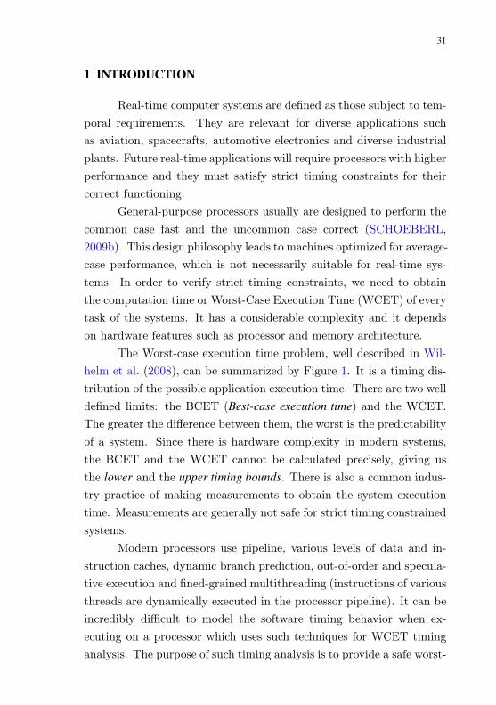
Real-time computer systems are defined as those subject to tem-poral requirements. They are relevant for diverse applications suchas aviation, spacecrafts, automotive electronics and diverse industrialplants. Future real-time applications will require processors with higherperformance and they must satisfy strict timing constraints for theircorrect functioning.
General-purpose processors usually are designed to perform thecommon case fast and the uncommon case correct (SCHOEBERL,2009b). This design philosophy leads to machines optimized for average-case performance, which is not necessarily suitable for real-time sys-tems. In order to verify strict timing constraints, we need to obtainthe computation time or Worst-Case Execution Time (WCET) of everytask of the systems. It has a considerable complexity and it dependson hardware features such as processor and memory architecture.
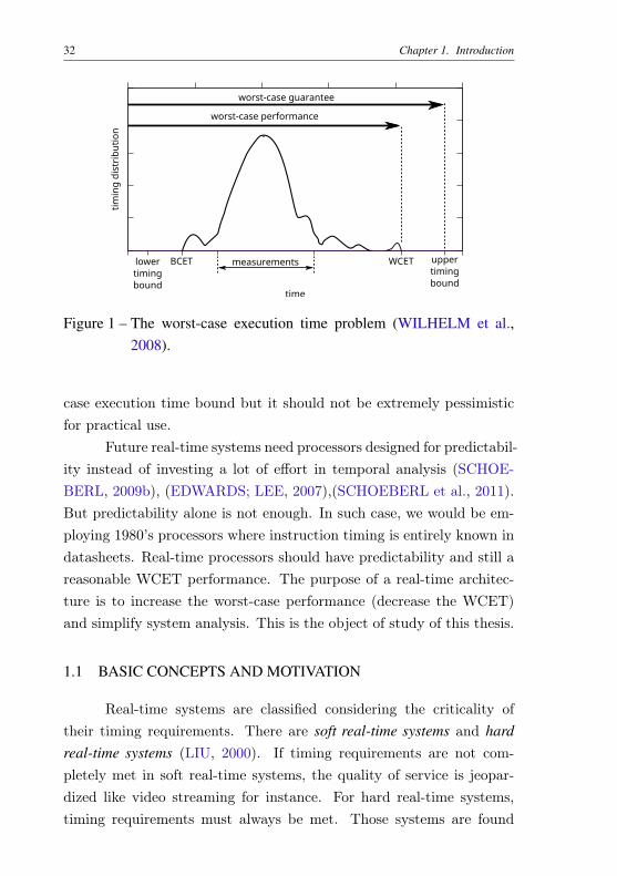
The Worst-case execution time problem, well described in Wil-helm et al. (2008), can be summarized by Figure 1. It is a timing dis-tribution of the possible application execution time. There are two welldefined limits: the BCET (Best-case execution time) and the WCET.The greater the difference between them, the worst is the predictabilityof a system. Since there is hardware complexity in modern systems,the BCET and the WCET cannot be calculated precisely, giving usthe lower and the upper timing bounds. There is also a common indus-try practice of making measurements to obtain the system executiontime. Measurements are generally not safe for strict timing constrainedsystems.
Modern processors use pipeline, various levels of data and in-struction caches, dynamic branch prediction, out-of-order and specula-tive execution and fined-grained multithreading (instructions of variousthreads are dynamically executed in the processor pipeline). It can beincredibly difficult to model the software timing behavior when ex-ecuting on a processor which uses such techniques for WCET timinganalysis. The purpose of such timing analysis is to provide a safe worst-
32 Chapter 1. Introduction
timin
g di
stri
butio
n
time
BCET WCETlowertimingbound
uppertimingbound
worst-case guarantee
worst-case performance
measurements
Figure 1 – The worst-case execution time problem (WILHELM et al.,2008).
case execution time bound but it should not be extremely pessimisticfor practical use.
Future real-time systems need processors designed for predictabil-ity instead of investing a lot of effort in temporal analysis (SCHOE-BERL, 2009b), (EDWARDS; LEE, 2007),(SCHOEBERL et al., 2011).But predictability alone is not enough. In such case, we would be em-ploying 1980’s processors where instruction timing is entirely known indatasheets. Real-time processors should have predictability and still areasonable WCET performance. The purpose of a real-time architec-ture is to increase the worst-case performance (decrease the WCET)and simplify system analysis. This is the object of study of this thesis.
1.1 BASIC CONCEPTS AND MOTIVATION
Real-time systems are classified considering the criticality oftheir timing requirements. There are soft real-time systems and hardreal-time systems (LIU, 2000). If timing requirements are not com-pletely met in soft real-time systems, the quality of service is jeopar-dized like video streaming for instance. For hard real-time systems,timing requirements must always be met. Those systems are found
1.1. Basic concepts and motivation 33
in critical applications like aviation or space systems where temporalfailures could lead to catastrophic consequences.
Real-time systems are modeled by tasks which are abstractions ofworks competing for resources. Tasks are comprised by timing parame-ters like WCET (C), maximum activation frequency or period (T ) anddeadline (D). The feasibility of a system is verified through schedu-lability analysis where it is ensured that all deadlines are respected.There is a lot of scheduling approaches for real-time systems (DAVIS;BURNS, 2011) and knowledge of the tasks WCET is always a concern.
The importance of obtaining the WCET of each task for systemanalysis is not a new problem. The question is how to estimate thisfundamental parameter for systems where they are not only restrictedto strict timing constraints but reasonable WCET performance is alsorequired. This is the main motivation of this work where we will investi-gate processor architecture features capable of guaranteeing timing pre-dictability, timing composability and increasing WCET performance.
1.1.1 Timing anomalies
The term anomaly denotes a deviation of the expected behaviorfrom the real behavior. A timing anomaly is the unexpected deviationof real hardware behavior compared with the model used during tempo-ral analysis (WENZEL et al., 2005). Predictions from models becomewrong and this could lead to erroneous calculation results by WCETanalysis methods. Thus, the concept of timing anomalies rather relatesto WCET analysis and does not denote malicious behavior during ex-ecution.
WCET analysis is commonly performed in many phases. Onephase is responsible for the processor hardware modeling and it com-putes upper bounds for program code snippets called basic blocks. Thetiming of each block is usually calculated independently from the othersand it must consider an initial state. Due to lack of state information(the processor model may contain simplifications), it is assumed theworst behavior of hardware components (e.g. cache misses). Due to
34 Chapter 1. Introduction
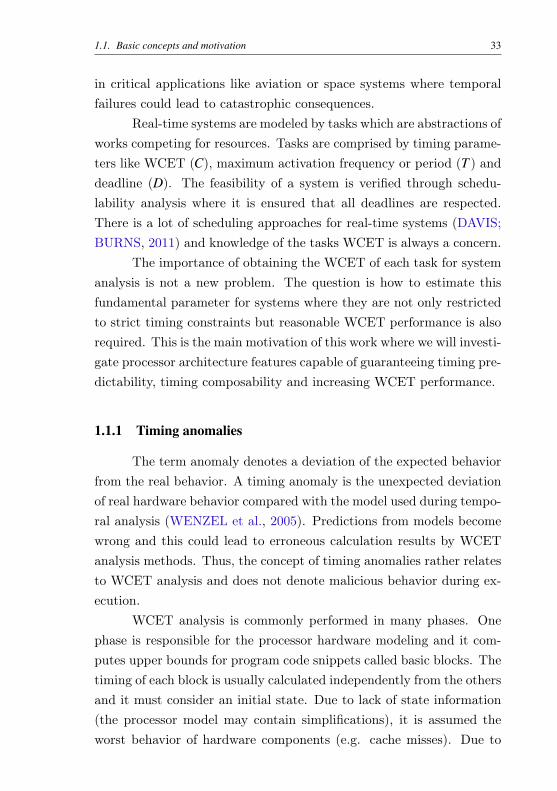
timing anomalies, assuming local worst case not necessarily means thatthe worst computation time is calculated. Figure 2 illustrates an ex-ample of timing anomaly. A cache hit in code snippet “a” triggers aprefetch. This prefetch evicts the contents of snippet “b” and the ex-ecution of a→ b takes 8 cycles. On the other side, if there is a missin “a” , there is no eviction of “b” and the execution of a→ b takes 5cycles. This simple example demonstrates that local worst case of “a”does not necessarily produces the global worst case of a→ b executiondue to a simple 3-cycle prefetch.
cycle
Cache MISS in a
Cache HIT in a
0 1 2 3 4 5 6 7 8
prefetch evicts cache contents of b
Figure 2 – Example of timing anomaly. Adapted from (WENZEL et al.,2005).
Timing anomalies are common for dynamic scheduling in out-of-order processors (LUNDQVIST; STENSTROM, 1999). There aremethods to analyze this type of architecture but usually they lead tooverestimations or extremely complex approaches. Sometimes proces-sor features (like dynamic branch prediction) must be disabled to guar-antee a feasible WCET calculation.
1.1.2 Timing predictability
A real-time system is not necessarily a high-performance system.A common error is to assume that a task has to run on a fast proces-sor to meet its deadline. Fast processors usually improve average-caseperformance but can easily jeopardize the WCET analysis due to pre-dictability issues.
To make sure that all tasks of the system meet their respec-tive deadlines, it is necessary to determine the WCET of each one.
1.1. Basic concepts and motivation 35
This is possible if the hardware is time predictable or time analyzable.This two concepts are formalized in (GRUND; REINEKE; WILHELM,2011). Predictability is not a Boolean property. It should be expressedby ranges allowing the comparison of systems, i.e., system X is morepredictable than Y . Moreover it considers some level of accuracy andthe maximum level is obtained when the system can be exactly pre-dicted. Analyzability is how the system timing is modeled and it indi-cates the capacity of this modeling to predict timing properties.
There are other predictability definitions as the one described in(THIELE; WILHELM, 2004). They use the difference between the real(exact) WCET and the estimated upper bound. Later, in (KIRNER;PUSCHNER, 2010), they used the range between real BCET and realWCET where a lower range implies a better predictability and BCETequals to WCET is the maximum achievable predictability.
Predictability definitions/quantifications that use exact valuesof WCET/BCET may be impractical because they actually cannot beknown, only estimated (SCHOEBERL, 2012). Systems should be com-pared considering three basic aspects: hardware, compiler and WCETanalysis tool. The relevance of two of them can be characterized as fol-lows. A task τ has 1000 WCET cycles running on processor A, but 800WCET cycles running on processor B (considering hypothetically bothexact WCET values). Clearly, if we know those exact WCET values,processor B is better than A. Unfortunately, the WCET estimation isperformed by a tool Sa for processor A and another tool Sb for processorB and their estimated upper bounds are 1100 cycles and 1300 cyclesfor A and B respectively. Now processor A is better. If predictabilityis estimated by WCET real
WCET bound for instance, PA = 0.91 and PB = 0.61, A ismore predictable than B and the tool Sa is also better. An efficiencyproblem arises if tool Sa takes one day and tool Sb takes minutes toestimate the WCET of task τ .
As we can see, the notion of predictability should capture whethera specified property of a system can be predicted by an optimal anal-ysis and to what level of precision (GRUND; REINEKE; WILHELM,2011)
36 Chapter 1. Introduction
1.1.3 Timing composabilty
The complexity and the level of the requirements of real-timesystems are reasonable nowadays. It is necessary to analyse the sys-tem to verify if timing requirements are met. But as described in(PUSCHNER; KIRNER; PETTIT, 2009), there is a lack of methodsand tools to effectively reason about the timing of software. It is dif-ficult for real-time software systems to be constructed hierarchicallyfrom components while still guaranteeing timing properties. To achievea hierarchical construction, system components should be both com-posable and compositional from the timing perspective. Composabilityfocuses on preservation of properties of an individual component whenit is integrated in an application and compositionality is the ability ofdeducing global properties of the composed system from properties ofits constituent modules (MARTÍNEZ; CUEVAS; DRAKE, 2012). Be-sides compositionality and composability, other properties should bepresent (PUSCHNER; KIRNER; PETTIT, 2009) to achieve a com-posable timing analysis: support for hierarchical development process,predictability, scalability and performance.
Most hardware architectures used today can not provide theproperties listed by (PUSCHNER; KIRNER; PETTIT, 2009). Re-garding composability, real-time tasks executing on the same hardwarecompete for resources whose access times are state-dependent such asdata cache memories and branch buffers (used in branch prediction).The state of these resources depends on the data addresses and onthe access history. We can see that state depends on spatial and tem-poral aspects and, of course, the update strategy because both cacheand branch buffers have space limitations. The use of those hardwaremechanisms degrade composability because the property of an individ-ual module or task is not preserved when it is integrated with othertasks. The lack of composability when using branch prediction anddata cache memories degrades scalability as well because branch pre-diction interferes with cache contents. WCET analysis must considerboth branch directions when the analysis cannot anticipate the outcome
1.2. Thesis objective 37
of the prediction.Composability and predictability are also greatly affected in the
presence of timing anomalies. Timing anomalies related to WCETanalyses were first described by (LUNDQVIST; STENSTROM, 1999).A timing anomaly is a situation where the local worst case does notcontribute to the global worst case, i.e., a cache miss, though increasingthe execution time, results in shorter global execution time. The firstcondition to avoid timing anomalies is the use of in-order resources(LUNDQVIST; STENSTROM, 1999) what is not common in todayhardware architectures. Timing anomalies jeopardize the composabil-ity because we cannot divide WCET calculation in subproblems. Pre-dictability is also affected because simplifications on the analyses willnot produce results with a reasonable accuracy margin.
In order to guarantee a composable timing analysis, state-of-the-art processor technologies such as dynamic branch prediction andcache memories with out-of-order pipelines should be avoided. Yet, asstated by (PUSCHNER; KIRNER; PETTIT, 2009), strategies adoptedin real-time architectures should not lead to significant performancelosses when compared to state-of-the-art technologies.
1.2 THESIS OBJECTIVE
The objective of this thesis is to investigate various processorarchitecture features that lead to a predictable design with reasonableWCET performance. The thesis to be demonstrated is that it is possi-ble to assemble together hardware elements that increase performancebut are predictable enough to ensure efficient and precise analyses. Asdescribed in the previous section, one of the first steps to demonstratepredictability is by obtaining the WCET. The construction of a WCETanalysis tool as well as aspects involved with the hardware are also sub-jects of this work.
Among the architectural elements that are covered, we have:
∙ Processor pipeline:
38 Chapter 1. Introduction
Pipelining is a technique where complex operations are organizedinto sequential simpler ones to increase throughput. In the caseof predictable processor design, pipelines are necessary but in-structions should be executed in-order. Pipelines with out-of-order execution allow high average-case performance but jeop-ardize WCET analysis due to timing anomalies (LUNDQVIST;STENSTROM, 1999).
∙ Instruction parallelism:
In modern processor design, the concept of superscalar is exten-sively used where more than one instruction is executed in eachpipeline stage. This design overcomes the limitation of standardpipelines where the maximum throughput is one instruction percycle. In the case of real-time processors, multiple instructionscould also be executed in each pipeline stage using the Very LongInstruction Word (VLIW) design philosophy (FISHER; FARA-BOSHI; YOUNG, 2005). VLIW machines are better for real-timesystems because instruction scheduling is fixed and defined offlineduring compilation time and, that enhances the analyzability. Nohardware for instruction scheduling have to be modeled in VLIWdesign.
∙ First level of the memory subsystem:
Memory subsystems designed for real-time systems are the sub-ject of various recent works (REINEKE et al., 2011). There areseveral approaches and some of them require complex modifica-tions in the compiler and/or overload the hardware (SCHOE-BERL et al., 2011). In this work, we will address the memorypredictability issues using a direct-mapped instruction cache anda scratchpad memory for data. Scratchpad memories are simi-lar to caches but their contents must be managed explicitly bysoftware.
∙ Branch prediction:
1.2. Thesis objective 39
Branches are instructions that perform conditional control-flowmodifications. They are used for if, for and while structures andthey usually decrease pipeline performance adding stall cycles tothe pipeline. One way to overcome this limitation is the use ofbranch prediction. There are dynamic branch predictions andstatic branch predictions. The use of dynamic branch predictionsjeopardizes predictability and the static ones provide interestingWCET performance (BURGUIERE; ROCHANGE; SAINRAT,2005). We support static branch prediction demonstrating itsimportance in terms of performance and we provide methods forcorrect WCET analyzability.
∙ Predication:
Predication is a technique where instructions are conditionally ex-ecuted based on a Boolean register. It is different from branchesbecause there is not any control flow modification to execute orignore instructions. There are two types of predication: partialand full. Full predication allows instructions to be executed orignored directly based on a Boolean register (this type of predi-cation is common in ARM architectures). In case of partial pred-ication, instructions cannot be ignored through a Boolean oper-ator but two values can be selected using special select instruc-tions. Predication is an important technique to reduce programpaths through inducing to the single-path programming paradigm(PUSCHNER, 2005). We support both partial and full predica-tion but the latter is simplified to improve WCET analysis with-out jeopardizing performance.
∙ Complex arithmetic instructions:
There are complex arithmetic instructions like division and mul-tiplication that impose considerable overhead to the processorpipeline. Frequently, those instructions are only supported viasoftware, mainly division. In this work we support both hard-
40 Chapter 1. Introduction
ware division and multiplication and they are implemented tohave constant timing independently of their input parameters.
We conduct a study of the impact on the WCET performanceof those processor features that are typically disabled or not fully ex-plored in real-time applications. Such features include the use of staticscheduling VLIW processor with wide fetch, the importance of staticbranch prediction, the performance of complex instructions (memory,multiplications, division) and the use of predication.
Increasing the performance of real-time processors while preserv-ing analyzability is a relevant subject. For that purpose, we analyzethe WCET performance of the deterministic four-issue Very Long In-struction Word (VLIW) processor prototype describing its features andits timing characteristics. This prototype is implemented in VHDL us-ing an Altera Cyclone IV GX (EP4CGX150DF31C7) in a DE2i-150development board.
Besides the VHDL prototype, there are other products of thisthesis like the implementation of the hardware modeling of the WCETanalysis tool and cycle accurate software simulator. Both WCET anal-ysis tool and the simulator are written in C++. In order to have acompiler for the architecture and to provide a customizable environ-ment to research real-time compiler capabilities, a new code generatorback-end for LLVM (LATTNER; ADVE, 2004) was implemented butit is out of the scope of this thesis.
In terms of test cases, we used representative examples of Mälar-dalen WCET benchmarks (GUSTAFSSON et al., 2010) which are com-monly used for WCET evaluations.
1.3 CONTRIBUTIONS
Regarding our main contributions to real-time processor archi-tectures, we can highlight:
∙ Design space investigation and evaluation:
1.4. Text organization 41
We made a complete evaluation of the proposed techniques andwe highlighted their performance benefits.
∙ Complete WCET analysis for the proposed design:
We present all necessary analyses to perform WCET estimationsof programs compiled for the design proposed in this thesis. Suchanalyses include cache modeling, pipeline modeling and worst-case path search. An integrated environment between WCETand compiler is utilized to enhance WCET estimation.
∙ Complete VHDL design and timing characterization:
We describe the implementation of the researched approaches re-garding our deterministic real-time processor. We describe thetiming of each module and their VHDL implementation, whichare necessary for WCET modeling and estimation.
∙ Detailed branch architecture:
All details of the branch architecture are described including ourmethodology to model it during WCET analyses. We also ex-tended the ISA to support static branch prediction and estimatedthe performance benefits of using or not this technology in real-time systems.
∙ Low overhead full predication system for VLIW processors:
We propose a low-overhead full-predication system without addingoverhead to the hardware data paths or its forwarding logic. Theproposed predication system enhances the support of the singlepath execution as well as loop unrolling techniques.
1.4 TEXT ORGANIZATION
This thesis is organized in eight chapters including the Introduc-tion which covers some basic concepts about predictability considera-tions, our main motivation and the thesis objective.
42 Chapter 1. Introduction
Chapter 2 describes techniques employed in modern processorsand how they affect hardware predictability. Pipeline principles, in- andout-of-order execution, branch prediction and predication are topics inthe scope of this chapter.
Chapter 3 presents a list of related researches with their maincontribution and objectives.
Chapter 4 is the core of this thesis. We describe the thesis ratio-nale and the problem defining our target system and its requirements.We discuss design decisions for the proposed architecture comparingthem with the related researches and we highlight our contributions.
Chapter 5 presents the VHDL hardware implementation of thedesign. This chapter is important because the implementation is thearchitecture realization of the proposed design. With this realization, wecan infer hardware complexity of each component and the timing of theprocessor. The timing behavior is important for the WCET estimationwhich is covered in Chapter 6. This particular chapter describes howwe propose to analyze the processor using composability. Instructioncache modeling, pipeline analysis and worst-case path search are topicsin the scope of this chapter.
Chapter 7 describes our evaluation methodology. We assess theimpact of architecture techniques upon WCET performance. The mainidea is to quantitatively show WCET performance gains consideringfeatures employed in our design such as wide instruction fetching, la-tency of memory operations, static branch prediction and predication.
Finally, Chapter 8 presents our final remarks and suggestions forfuture work.
43
2 PROCESSORS AND PREDICTABILITY CONSIDERATIONS
In this chapter we briefly describe some important processor as-pects that will be used throughout this thesis. We also consider theimpact of using those techniques in the design of a processor suitablefor future real-time systems.
The design and specification of a microprocessor include its In-struction Set Architecture (ISA). It specifies what instructions the pro-cessor can execute. The hardware implementation is characterized by aHardware Description Language (HDL) and it describes simple Booleanlogic (logic gates), registers and more complex structures such as de-coders and multiplexers. Entire functional modules such as adder andmultiplier circuits can be developed with these HDL structures.
Literature usually defines three abstraction levels (SHEN et al.,2005) for computer architectures: architecture, implementation and re-alization. The architecture specifies the ISA and defines the fundamen-tal processor behavior. All software must be encoded using such ISA.Some examples of ISA are MIPS32, AMD x86_64, ARM e ST200. Theimplementation specifies the project of the architecture, known as mi-croarchitecture. The implementation is responsible for pipeline, cachememories and branch prediction specifications. The realization of aprocessor implementation is the physical encapsulation. In the caseof microprocessors, this encapsulation is the chip. Realizations canvary depending on operating frequency, cache memory capacity, buses,lithography and packing. Realization also impacts on attributes as diesize, power and reliability.
The ISA also defines a contract between the software and thehardware. This contract leads to an independent software and hard-ware development. Programs encoded using a particular ISA can beexecuted on different implementations with different levels of perfor-mance.
44 Chapter 2. Processors and predictability considerations
2.1 PIPELINE PRINCIPLES
Pipelining is a powerful technique to increase performance with-out massive hardware replication. Its main purpose is to increase theprocessor throughput with a low hardware increment. Throughput isthe amount of instructions performed per unit of time – Instructionsper cycle (IPC) . If a processor performs one instruction per unit oftime, its throughput is 1/D where D is the instruction’s latency. Whenusing a pipeline, the processor subsystem is decomposed between sev-eral multiple simple stages adding a memory (buffer) between each ofthose stages. The original instruction is now composed of k stages anda new instruction can be initialized immediately after the previous onereaches the second stage. Instead of issuing an instruction after D unitsof time, the processor issues a new one after D/k units of time and theinstructions are overlapped along the pipeline stages.
The performance improvement is ideally proportional to the pipe-line length. However, there are physical limitations that reduce thenumber of feasible pipeline stages. In general, the limit of how a syn-chronous system can be divided into stages is associated with the mini-mum time required for the circuit operation: the uncertainty associatedon using high frequencies and the distribution of circuit delays. Besidesphysical limitations, there is a cost and performance ratio that deter-mines the optimal number of pipeline stages for a processor (SHEN etal., 2005) since hardware needs to be added for each added pipelinestage.
There are three basic challenges on using pipelines:
∙ Pipeline stages should be balanced to provide uniform sub-computa-tions with same latency.
∙ Instructions should be unified to provide identical sub-computationsusing all stages.
∙ Instructions should be independent to reduce pipeline stalls.
2.1. Pipeline principles 45
Uniform sub-computations with the same latency reduce internalpipeline fragmentation. It is difficult to provide perfect and balancedstages and the pipeline operating frequency will be associated with thestage with higher latency. Processors also execute different types ofinstructions and not all of them will require all stages to execute. Sinceusually it is not possible to unify all sub-computations for all typesof instructions, some degree of external fragmentation will exist andinstructions need to pass every pipeline stage even if a particular stageis not required. If all computations were independent, a pipeline couldoperate in a continuous stream and it achieves to maximum throughput.Unfortunately, processor instructions are not fully independent and theresult of one instruction could be required for the computation of thenext one. If there is no hardware mechanism to forward this result tothe next instruction, the pipeline must stall to guarantee instructionsemantics.
One generic 5-stage pipeline is naturally formed by one basicinstruction cycle divided into the next five generic sub-computations:
1. Fetching (F).
2. Decoding (D).
3. Executing (E).
4. Memory accessing (M).
5. Results writing back (WB).
This generic pipeline begins with an instruction being fetchedfrom memory. Next, it is decoded to determine which type of work willbe performed and one or more operators are fetched from the processorregisters. As soon as the operators are available, the decoded instruc-tion is executed and the cycle ends by writing back the result in thememory or in the registers. During these five generic sub-computations,some exceptions can occur by changing the machine state and they arenot explicitly specified in the instruction. The complexity and latencyof each stage varies significantly depending on the processor’s ISA.
46 Chapter 2. Processors and predictability considerations
Considering a modern RISC processor, the generic 5-stage pipelineexecutes three basic instructions classes:
1. Arithmetic and logical instructions (add, sub, shift) – performedby an ALU (Arithmetic Logical Unit);
2. Memory instructions (load/store): performed by a memory unitthat moves data between register and memory;
3. Control flow instructions (branch, calls and jumps): performedby a branch unit that manipulates the control flow.
Arithmetic instructions are restricted only to processor registeroperands. Only memory instructions access the memory. These restric-tions form a load/store RISC architecture. Control flow instructionsare used to manipulate the control flow to support function calls/re-turns as well as loop, if-then-else and while structures. They usuallyuse relative addressing and the calculation of target address uses theprogram counter (PC) as reference.
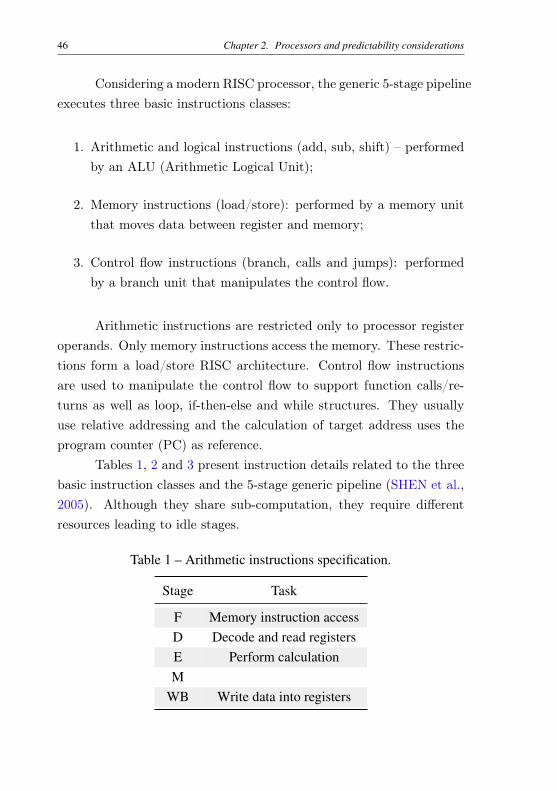
Tables 1, 2 and 3 present instruction details related to the threebasic instruction classes and the 5-stage generic pipeline (SHEN et al.,2005). Although they share sub-computation, they require differentresources leading to idle stages.
Table 1 – Arithmetic instructions specification.
Stage Task
F Memory instruction accessD Decode and read registersE Perform calculationM
WB Write data into registers
2.1. Pipeline principles 47
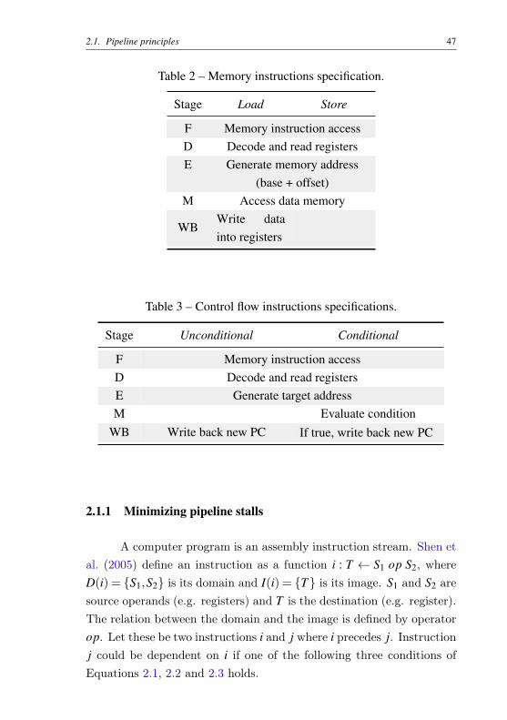
Table 2 – Memory instructions specification.
Stage Load Store
F Memory instruction accessD Decode and read registersE Generate memory address
(base + offset)M Access data memory
WBWrite datainto registers
Table 3 – Control flow instructions specifications.
Stage Unconditional Conditional
F Memory instruction accessD Decode and read registersE Generate target addressM Evaluate condition
WB Write back new PC If true, write back new PC
2.1.1 Minimizing pipeline stalls
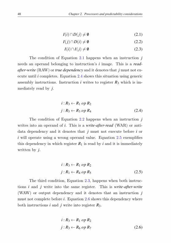
A computer program is an assembly instruction stream. Shen etal. (2005) define an instruction as a function i : T ← S1 op S2, whereD(i) = {S1,S2} is its domain and I(i) = {T} is its image. S1 and S2 aresource operands (e.g. registers) and T is the destination (e.g. register).The relation between the domain and the image is defined by operatorop. Let these be two instructions i and j where i precedes j. Instructionj could be dependent on i if one of the following three conditions ofEquations 2.1, 2.2 and 2.3 holds.
48 Chapter 2. Processors and predictability considerations
I(i)∩D( j) ̸= /0 (2.1)
I( j)∩D(i) ̸= /0 (2.2)
I(i)∩ I( j) ̸= /0 (2.3)
The condition of Equation 2.1 happens when an instruction jneeds an operand belonging to instruction’s i image. This is a read-after-write (RAW) or true dependency and it denotes that j must not ex-ecute until i completes. Equation 2.4 shows this situation using genericassembly instructions. Instruction i writes to register R3 which is im-mediately read by j.
i : R3← R1 op R2
j : R5← R3 op R4 (2.4)
The condition of Equation 2.2 happens when an instruction jwrites into an operand of i. This is a write-after-read (WAR) or anti-data dependency and it denotes that j must not execute before i ori will operate using a wrong operand value. Equation 2.5 exemplifiesthis dependency in which register R1 is read by i and it is immediatelywritten by j.
i : R3← R1 op R2
j : R1← R4 op R5 (2.5)
The third condition, Equation 2.3, happens when both instruc-tions i and j write into the same register. This is write-after-write(WAW) or output dependency and it denotes that an instruction jmust not complete before i. Equation 2.6 shows this dependency whereboth instructions i and j write into register R3.
i : R3← R1 op R2
j : R3← R6 op R7 (2.6)
2.1. Pipeline principles 49
All above dependencies must be respected to ensure correct pro-gram semantics. Pipelines could easily break instruction semantics andthere must be mechanisms for identifying and resolving them. A po-tential dependency violation is known as a pipeline hazard.
D:
E:
M:
WB:
F:
D
E
M
F
WB
ALU Load Store Branch
Arithmeticexecution
Registerswrite back
Address generation
Memoryread
Instruction fetch
Instruction decoding and register reading
Memory write
PCupdate
Branchevaluation
PC update
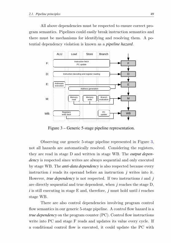
Figure 3 – Generic 5-stage pipeline representation.
Observing our generic 5-stage pipeline represented in Figure 3,not all hazards are automatically resolved. Considering the registers,they are read in stage D and written in stage WB. The output depen-dency is respected since writes are always sequential and only executedby stage WB. The anti-data dependency is also respected because everyinstruction i reads its operand before an instruction j writes into it.However, true dependency is not respected. If two instructions i and jare directly sequential and true dependent, when j reaches the stage D,i is still executing in stage E and, therefore, j must hold until i reachesstage WB.
There are also control dependencies involving program controlflow semantics in our generic 5-stage pipeline. A control flow hazard is atrue dependency on the program counter (PC). Control flow instructionswrite into PC and stage F reads and updates its value every cycle. Ifa conditional control flow is executed, it could update the PC with
50 Chapter 2. Processors and predictability considerations
the target address on true condition or the next linear address couldbe fetched on false. Since the control flow instructions update the PConly in the stage WB, there is a true dependency violation because PCis read before WB updates the new address.
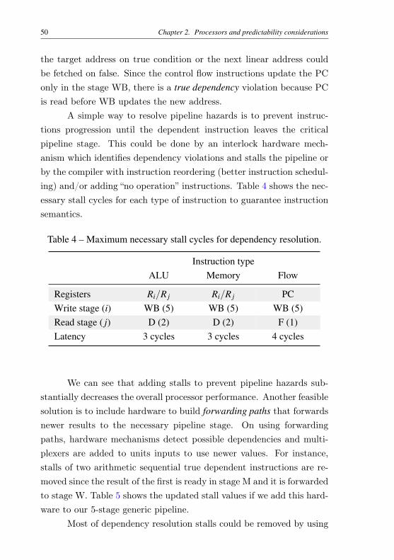
A simple way to resolve pipeline hazards is to prevent instruc-tions progression until the dependent instruction leaves the criticalpipeline stage. This could be done by an interlock hardware mech-anism which identifies dependency violations and stalls the pipeline orby the compiler with instruction reordering (better instruction schedul-ing) and/or adding “no operation” instructions. Table 4 shows the nec-essary stall cycles for each type of instruction to guarantee instructionsemantics.
Table 4 – Maximum necessary stall cycles for dependency resolution.
Instruction typeALU Memory Flow
Registers Ri/R j Ri/R j PCWrite stage (i) WB (5) WB (5) WB (5)Read stage ( j) D (2) D (2) F (1)Latency 3 cycles 3 cycles 4 cycles
We can see that adding stalls to prevent pipeline hazards sub-stantially decreases the overall processor performance. Another feasiblesolution is to include hardware to build forwarding paths that forwardsnewer results to the necessary pipeline stage. On using forwardingpaths, hardware mechanisms detect possible dependencies and multi-plexers are added to units inputs to use newer values. For instance,stalls of two arithmetic sequential true dependent instructions are re-moved since the result of the first is ready in stage M and it is forwardedto stage W. Table 5 shows the updated stall values if we add this hard-ware to our 5-stage generic pipeline.
Most of dependency resolution stalls could be removed by using
2.1. Pipeline principles 51
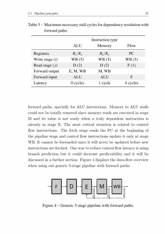
Table 5 – Maximum necessary stall cycles for dependency resolution withforward paths.
Instruction typeALU Memory Flow
Registers Ri/R j Ri/R j PCWrite stage (i) WB (5) WB (5) WB (5)Read stage ( j) D (2) D (2) F (1)Forward output E, M, WB M, WBForward input ALU ALU FLatency 0 cycles 1 cycle 4 cycles
forward paths, specially for ALU instructions. Memory to ALU stallscould not be totally removed since memory reads are executed in stageM and its value is not ready when a truly dependent instruction isalready in stage E. The most critical situation is related to controlflow instructions. The fetch stage reads the PC at the beginning ofthe pipeline stage and control flow instructions update it only at stageWB. It cannot be forwarded since it will never be updated before newinstructions are fetched. One way to reduce control flow latency is usingbranch prediction but it could decrease predictability and it will bediscussed in a further section. Figure 4 displays the data-flow overviewwhen using our generic 5-stage pipeline with forward paths.
F E M WBD
ULA
to U
LA
MEM
to U
LA
WB
to U
LA
Figure 4 – Generic 5-stage pipeline with forward paths.
52 Chapter 2. Processors and predictability considerations
2.2 MULTIPLE INSTRUCTION FETCHING
Pipelines described in the previous section reach a theoreticalk speed-up factor where k is the number of stages. Their maximumthroughput could also reach about 1 instruction per cycle (IPC). In-stead of dividing the work in k simpler stages, we can reach this per-formance replicating the work with k copies allowing a different type ofinstruction level parallelism (ILP). Standard pipelines provide temporalparallelism while allowing multiple instruction execution give us spatialparallelism. If temporal and spatial parallelism are combined, proces-sors could reach more than one instruction per cycle. Pipelining alliedwith wider instruction fetch constitute superscalar and VLIW (VeryLong Instruction Word) machines. Both types of machines providehigher ILP and the basic difference between them is related to instruc-tion scheduling. In superscalar machines, the hardware is responsiblefor instruction scheduling while in VLIW machines, instructions arestatically scheduled by the compiler.
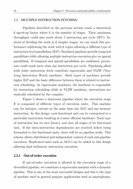
Figure 5 shows a dual-issue pipeline where the execution stageE is composed of different types of execution units. This machinecan, for instance, execute at the same time one ALU and one memoryinstruction. In this design, each functional unit can be customized to aparticular instruction resulting in a more efficient hardware. Each typeof instruction has its own latency and uses all stages of its functionalunit. If the intra-instruction dependencies are resolved before beingforwarded to the functional units, there will be no pipeline stalls. Thisscheme allows distributed and independent control of each sub-pipelineexecution. Replicated units such as ALUs can be added to this designallowing dual arithmetic instruction execution.
2.2.1 Out-of-order execution
If out-of-order execution is allowed in the execution stage of adiversified pipeline, we constitute a superscalar machine with a dynamicpipeline. This is one of the most successful designs and this is the typeof machine used in general purpose applications such as smartphones,
2.2. Multiple instruction fetching 53
F
E
D
M1
M2
ALU FP1
FP2
FP3
Br1
Br2
WB
Figure 5 – Diversified pipeline example: Mx are memory sub-stages, FPx
are floating-point stages and BRx are branch stages.
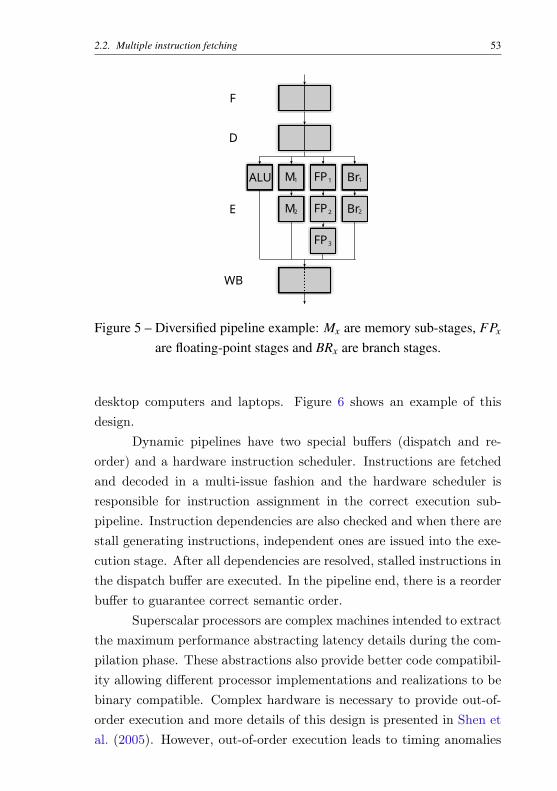
desktop computers and laptops. Figure 6 shows an example of thisdesign.
Dynamic pipelines have two special buffers (dispatch and re-order) and a hardware instruction scheduler. Instructions are fetchedand decoded in a multi-issue fashion and the hardware scheduler isresponsible for instruction assignment in the correct execution sub-pipeline. Instruction dependencies are also checked and when there arestall generating instructions, independent ones are issued into the exe-cution stage. After all dependencies are resolved, stalled instructions inthe dispatch buffer are executed. In the pipeline end, there is a reorderbuffer to guarantee correct semantic order.
Superscalar processors are complex machines intended to extractthe maximum performance abstracting latency details during the com-pilation phase. These abstractions also provide better code compatibil-ity allowing different processor implementations and realizations to bebinary compatible. Complex hardware is necessary to provide out-of-order execution and more details of this design is presented in Shen etal. (2005). However, out-of-order execution leads to timing anomalies
54 Chapter 2. Processors and predictability considerations
F
E
D
M1
M2
ULA PF1
PF2
PF3
Br1
Br2
WB
in order
out of order
dispatch buffer
reorder buffer
out of order
in order
Figure 6 – Dynamic pipeline example: Mx are memory sub-stages, FPx
are floating-point stages and BRx are branch stages.
and the high hardware complexity leads to unbounded states duringWCET analysis.
2.2.2 In-order execution
Multiple instruction fetching with in-order execution and with-out hardware instruction scheduling leads to a VLIW (Very Long In-struction Word) design. The VLIW philosophy exposes the hardwarenot only at the ISA level but also at Instruction Level Parallelism (ILP).Superscalar machines extracted ILP using hardware features rearrang-ing operations not directly specified in the code. VLIW processors donot perform any instruction scheduling and ILP must be provided bythe compiler. Instruction rearranging (scheduling) is performed offlineduring compilation and the processor executes instructions exactly asdefined by the compiler. The main idea is not to let the hardware dothings that cannot be seen in programming, to reduce processor com-
2.2. Multiple instruction fetching 55
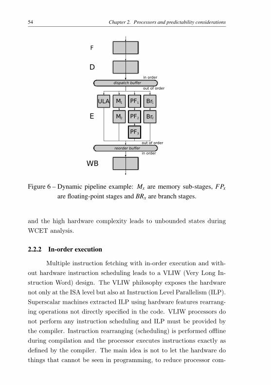
Table 6 – Basic differences between VLIW and Superescalar designs(FISHER; FARABOSHI; YOUNG, 2005).
Superescalar VLIW
Instructionflow
Multiple scalar opera-tions are fetched
Instructions are fetchedsequentially but withmultiple operations
Scheduling Hardware dynamicscheduler
Compiler static sched-uler
Fetch width Hardware dynamicallydetermines the numberof fetched instructions
Compiler determinesstatically the number offetched instructions
Instructionordering
Dynamic fetching al-lowing out-of-order andin-order execution
Static fetching withonly in-order execution
Implications Superescalar design isrelated to microarchi-tecture techniques
VLIW is an architec-tural technique. Hard-ware details are ex-posed to the compiler
plexity, to have only simple instructions and to increase predictabilitywhen needed. Table 6 shows basic differences between superscalar andVLIW designs.
VLIW designs are not commonly used in general purpose com-puting but they are very popular in embedded applications. SeveralDSPs (Digital Signal Processors) like Texas Instrument C6x, Agere/-Motorola StarCore, Suns’s MAJC, Fujitsu’s FR-V, STss HP/ST Lx(ST200), Philips’ Trimedia, Silicon Hive Avispa, Tensilica Xtensa Lxand Analog Devices TigerShark are VLIW processors. Intel’s Itaniumarchitecture for servers also uses this design philosophy.
VLIW compilers are more sophisticated since they must performoperations usually executed by the superscalar hardware. A superscalar
56 Chapter 2. Processors and predictability considerations
control unit avoids sophisticated compilers. The fact that all ILP ex-traction is done by the hardware every time an instruction is fetchedby the processor control unit shows that this work could be easily doneby the compiler. The code reordering after out-of-order execution isrelatively trivial and compilers can handle it easily and they can evolvefaster than a new processor construction.
Considering real-time systems, VLIW is a very interesting solu-tion since hardware modeling is considerably less complex, in-order exe-cution avoids timing anomalies and higher performance can be achievedusing multi-issue instruction fetching.
2.3 BRANCH PREDICTION
Conditional control flow instructions are usually responsible forif and loop program constructions and, unfortunately, they break theideal pipeline flow reducing performance. Since control flow dependen-cies cannot be forwarded, as showed in Section 2.1, branch predictiontechniques are commonly used to reduce this performance loss.
Instead of stalling the pipeline until the branch condition isevaluated and the target address computed, both are speculated andpipeline continues to execute a speculated path. This additional hard-ware is the branch predictor and it is responsible for condition/targetaddress speculation and the recovery if the wrong path is taken.
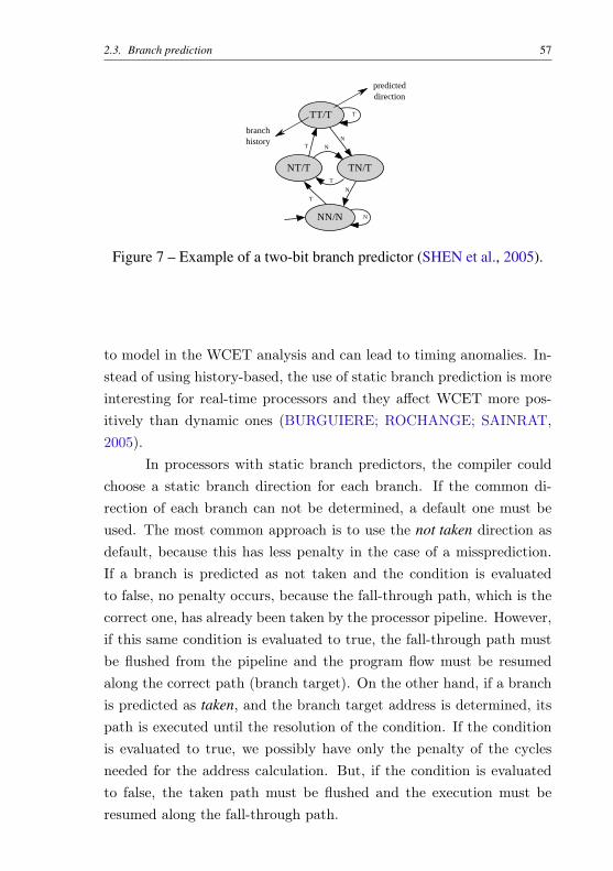
General purpose modern processors use advanced history basedbranch predictors. This type of dynamic predictor registers previouslybranch directions as taken (T) or not taken (N) and their addresses aswell. To predict the path of the next branch, this history is considered.History based predictors are very effective and they can predict 99% ofbranch directions (SHEN et al., 2005). Figure 7 illustrates the behaviorof a two-bit predictor. Two-bit states and target addresses for eachbranch are registered into hardware buffers known as Branch TargetBuffers (BTB) and they are essentially fully-associative caches.
Hardware elements which use execution history to increase per-formance are not very suitable for real-time systems. They are difficult
2.3. Branch prediction 57
NN/N N
NT/T
T
TT/T
T
TN/T
N
T
N
N
T
predicteddirection
branchhistory
Figure 7 – Example of a two-bit branch predictor (SHEN et al., 2005).
to model in the WCET analysis and can lead to timing anomalies. In-stead of using history-based, the use of static branch prediction is moreinteresting for real-time processors and they affect WCET more pos-itively than dynamic ones (BURGUIERE; ROCHANGE; SAINRAT,2005).
In processors with static branch predictors, the compiler couldchoose a static branch direction for each branch. If the common di-rection of each branch can not be determined, a default one must beused. The most common approach is to use the not taken direction asdefault, because this has less penalty in the case of a missprediction.If a branch is predicted as not taken and the condition is evaluatedto false, no penalty occurs, because the fall-through path, which is thecorrect one, has already been taken by the processor pipeline. However,if this same condition is evaluated to true, the fall-through path mustbe flushed from the pipeline and the program flow must be resumedalong the correct path (branch target). On the other hand, if a branchis predicted as taken, and the branch target address is determined, itspath is executed until the resolution of the condition. If the conditionis evaluated to true, we possibly have only the penalty of the cyclesneeded for the address calculation. But, if the condition is evaluatedto false, the taken path must be flushed and the execution must beresumed along the fall-through path.
58 Chapter 2. Processors and predictability considerations
2.4 PREDICATION
Predication is an architecture technique that helps the compilerto convert control dependencies into data dependencies. By using pred-icates, individual instructions can be deactivated by the Boolean valuewithout any program flow operation. This leads to conditional execu-tion or guarded execution (FISHER; FARABOSHI; YOUNG, 2005).
This is a powerful technology specially for real-time systems be-cause it gives the compiler the ability to reduce branch instructionsand avoid branch prediction side effects and possible pipeline hazards.Many modern processors use this technique and its use will be illus-trated by the simple C language code in Table 7. There are two typesof predication: full and partial. In full predication, an additional bitguard (px) is read for each instruction and if it is false, this particularinstruction is ignored. In partial predication, the processor’s ISA sup-ports a select or conditional move and a particular value is moved toits destination based on the bit guard. Table 7 shows the conditionalcode showed previously in normal mode (with branch), partial and fullpredication modes.
In the normal execution, the instruction at Line 1 makes thecomparison (cmpgt: compare greater than) assuming that variable xis in register r5 and the result is stored at the bit register p1. br fperforms a branch to L1 if p1 is false (brf: branch if false). We cannote that the multiplication at Line 4 is ignored using a control flow in-struction. Observing the full-predication execution, there is no controlflow operation and the multiplication (mull) is automatically ignored ifp1 is false. In the partial-predication, the multiplication is always exe-cuted at line 1 but its result is only considered if the select instruction(slct) at Line 4 moves the result to register r3 if p1 is true.
There are several works like (MAHLKE et al., 1995; CHOI etal., 2001) considering the predication for general purpose processorsand Intel’s Intanium has a very aggressive predication system. Be-sides helping to reduce control flow instructions, the average-case per-formance could be easily jeopardized because in both partial and full
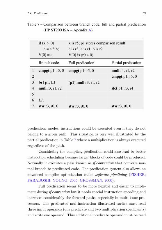
2.4. Predication 59
Table 7 – Comparison between branch code, full and partial predication(HP ST200 ISA – Apendix A).
if (x > 0) x is r5; p1 stores comparison resultc = a * b; c is r3; a is r1; b is r2
V[0] = c; V[0] is (r0 + 0)
Branch code Full predication Partial predication
1 cmpgt p1, r5, 0 cmpgt p1, r5, 0 mull r4, r1, r22 cmpgt p1, r5, 03 brf p1, L1 (p1) mull r3, r1, r24 mull r3, r1, r2 slct p1, r3, r456 L1:7 stw r3, r0, 0 stw r3, r0, 0 stw r3, r0, 0
predication modes, instructions could be executed even if they do notbelong to a given path. This situation is very well illustrated by thepartial predication in Table 7 where a multiplication is always executedregardless of the path.
Considering the compiler, predication could also lead to betterinstruction scheduling because larger blocks of code could be produced.Normally it executes a pass known as if conversion that converts nor-mal branch to predicated code. The predication system also allows anadvanced compiler optimization called software pipelining (FISHER;FARABOSHI; YOUNG, 2005; GROSSMAN, 2000).
Full predication seems to be more flexible and easier to imple-ment during if conversion but it needs special instruction encoding andincreases considerably the forward paths, especially in multi-issue pro-cessors. The predicated mul instruction illustrated earlier must readthree input operands (one predicate and two multiplication coefficients)and write one operand. This additional predicate operand must be read
60 Chapter 2. Processors and predictability considerations
every time an instruction is decoded and 3 bits of instruction encodingare lost if seven predicates are supported. The partial system, mean-while, needs only subtle ISA modifications adding few special condi-tional move instructions.
In the case of real-time systems, predication is important becauseit increases the code predictably and leads to programs with fewer paths(GEYER et al., 2013). The performance loss of the average case is alsonot an issue because real-time systems need performance of the worst-case scenario and fewer differences of the best-case, average-case andworst-case times lead to higher predictability.
2.5 CACHE MEMORIES
Cache memories are generally used to minimize the gap betweenprocessor and memory performances. Usually, main memory is slowerthan the processor so a fast cache is placed between them where mostrecent data is stored promoting faster access.
A cache memory is characterized by its capacity, line size andassociativity. Capacity is the caches’ total number of bytes; line size isthe quantity of bytes transferred from memory to cache when a cachemiss occurs. A cache could have n = capacity
line. size lines. Caches are muchsmaller than main memory and associativity consists of the mappingof various main memory addresses to cache lines. A direct-mappedcache has unitary associativity, where a specific main memory addressis always mapped to the same cache line. If associativity is two, a mainmemory address is mapped to 2 different cache lines. When associativ-ity is not unitary some sort of replacement policy must exist to decidewhich line will have data eviction. There are basically three policiesimplemented in the cache design: FIFO (first in, first out), LRU (LeastRecently Used) and random.
Considering cache misses, there are three main causes:
∙ Compulsory misses or cold cache: they happen when there isthe first reference to a particular memory address. These are
2.6. Scratchpad Memory 61
fundamental misses and they cannot be completely avoided byany technique.
∙ Capacity misses: they happen when there is no space left in thecache to store a particular memory block. Increasing the cachesize can eliminate some or all of the capacity misses.
∙ Conflict misses: they happen due to imperfect allocation andmapping of memory blocks to cache lines. Changes in associativ-ity or indexing function can improve conflict misses.
Various cache levels could also be used in processor design withdifferent sizes and associativities. However, these complex cache de-signs are not suitable for real-time processors because they can easilyforbid WCET analysis due to complex cache interference and no deter-ministic data eviction (SCHOEBERL, 2009b). Shared instruction anddata caches should also be avoided. During worst-case cache analysis,accessed memory addresses must be predicted. Data from the instruc-tion memory are easier to determine if the call tree is known. However,dynamically allocated data (heap) are difficult to predict statically be-cause such addresses are only available at runtime. Without knowingthe address, a single access can influence all cache sets. Predictableeviction policies like LRU are also more suitable for real-time applica-tions.
2.6 SCRATCHPAD MEMORY
Scratchpad memories are designed with the same technology ofcache memories, but they do not implement hardware data manage-ment. On using scratchpads, the compiler must explicitly manage datamemory using static or dynamic allocation. When exposing the mem-ory hierarchy with scratchpads, more work must be done by the com-piler. However, timing of memory accesses depends only on which andhow many memory blocks are accessed and additional latencies or un-known states provided by the hardware controller are non-existent. The
62 Chapter 2. Processors and predictability considerations
predictability associated with utilizing scratchpads is very interestingfor real-time applications. Since hardware controllers are non-existent,this additional area can be used in order to increase scratchpad size.
Scratchpads and main memory address spaces are usually unifiedand transfers between them are performed by Direct Memory Access(DMA) protocols (BANAKAR et al., 2002). The difference betweenan access to the main memory and to the scratchpad is only theiraddresses. Furthermore, there is not any hardware coherence protocolbetween memories. If necessary, such coherence must be developed insoftware.
There are various methods of performing data management forscratchpads for real-time systems including analysis for preemptivemultitasking (WHITHAM et al., 2012). There are additional approachesthat favor static partitioning of the scratchpad among real-time tasks(WHITHAM; AUDSLEY, 2010).
2.7 CHIP MULTITHREADING
Chip multithreading is another technique to increase processorperformance. Typically, fine-grained multithreading is implementedwhere instructions of different threads are overlapped in the processorpipeline. The execution stage with various units is shared among mul-tithreading fetch units and instructions of diverse threads are executedin parallel. Since different execution contexts are necessary, generalpurpose registers and state registers are replicated by the number ofsupported hardware threads. If there is some resource contention, likea single memory unit for instance, threads are typically stalled untilthis resource is available. This is the basic principle of Intel’s Hyper-threading technology and a dual multithreading system behaves like adual core system for the operating system.
Fine-grained multithreading is possible for real-time systems ifthe hardware thread scheduler and resource contention protocols arewell defined and predictable. Round-robin scheduler and Timed Divi-sion Access (TDM) protocol are usually employed. Multithreading can
2.8. Chip Multiprocessing 63
also remove pipeline dependencies. If we have a five-stage pipeline withfive hardware threads, it is possible to remove all forward logic sincefor each pipeline stage there will be a different thread instruction exe-cuting and pipeline dependencies never occur. This is the fundamentalidea of the work of Liu et al. (2012). However, if the number of acti-vated threads is less than the number of hardware threads available,the number of instructions per cycle is severely penalized. Consideringa scenario with only one activated thread and five hardware threads,the number of instructions per cycle is only 0.2 since a newer instruc-tion can only be issued after the old one is completed. Memory accessfor multithreading systems should also be special to remove or decreasethread interference.
Some works like Schoeberl (2009b) criticize chip multithreadingfor real-time systems since its analysis is more complex and the repli-cated hardware could be used for chip multiprocessing.
2.8 CHIP MULTIPROCESSING
Most modern computer systems available today use processorswith a single chip and multiple cores. Commonly these cores share asingle main memory and they are developed with complex and largeshared caches. Memory consistency between cores is usually managedby hardware and there are complex internal chip networks to supportdata transfer and consistency between all cores.
Real-time systems with chip multiprocessing are also viable andthis is a tendency as the complexity of these systems grows. Unfor-tunately, the technology employed in general purpose computing doesnot apply for real-time systems because it increases average-case perfor-mance but predictability proprieties are lost. Shared caches and com-plex hardware networks make the WCET analysis unfeasible. Thereare several works like Schoeberl et al. (2015) dealing with multipro-cessor designs for real time. In most approaches Timed Division Ac-cess (TDM) protocols are accompanied by real-time networks and datatransfer between cores is explicitly managed.
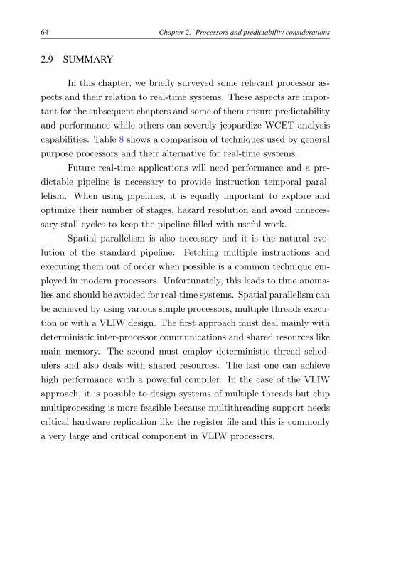
64 Chapter 2. Processors and predictability considerations
2.9 SUMMARY
In this chapter, we briefly surveyed some relevant processor as-pects and their relation to real-time systems. These aspects are impor-tant for the subsequent chapters and some of them ensure predictabilityand performance while others can severely jeopardize WCET analysiscapabilities. Table 8 shows a comparison of techniques used by generalpurpose processors and their alternative for real-time systems.
Future real-time applications will need performance and a pre-dictable pipeline is necessary to provide instruction temporal paral-lelism. When using pipelines, it is equally important to explore andoptimize their number of stages, hazard resolution and avoid unneces-sary stall cycles to keep the pipeline filled with useful work.
Spatial parallelism is also necessary and it is the natural evo-lution of the standard pipeline. Fetching multiple instructions andexecuting them out of order when possible is a common technique em-ployed in modern processors. Unfortunately, this leads to time anoma-lies and should be avoided for real-time systems. Spatial parallelism canbe achieved by using various simple processors, multiple threads execu-tion or with a VLIW design. The first approach must deal mainly withdeterministic inter-processor communications and shared resources likemain memory. The second must employ deterministic thread sched-ulers and also deals with shared resources. The last one can achievehigh performance with a powerful compiler. In the case of the VLIWapproach, it is possible to design systems of multiple threads but chipmultiprocessing is more feasible because multithreading support needscritical hardware replication like the register file and this is commonlya very large and critical component in VLIW processors.
2.9. Summary 65
Table 8 – Comparison of techniques for general-purpose and real-timeprocessors
Feature General purpose Real time
Pipeline Long with out-of orderexecution
Simple with in-orderexecution
Caches Complex with variouslevels, shared and com-plex associativities
Separate caches orscratchpad memory
Branch Dynamic predictors Static or non predictorsSuperscalability Multi-issue and out-of-
orderVarious simple coresor in-order multi issue(VLIW)
Chip multi-threading
Lots of hardwarethreads competing forshared resources
Avoid, use multiplecores or threads withinterleaved pipeline
Chip multipro-cessors
Shared caches withcore inter-interference
Separated cachesor scratchpads withpredictable core com-munication

67
3 RELATED WORK
The design of deterministic computer architectures for real-timesystems is very relevant and there are several works in this researchfield. Since high-performance general-purpose processors are not suit-able, it is desired to have new predictable architectures enhancing theWCET analyzability while not ignoring more stringent performancerequirements. The main concern is related to WCET analysis.
In this chapter we survey related work on predictable architec-tures. Compiler techniques, timing analysis techniques and architec-tural techniques are all important for the predictability of computerarchitectures. However, we focus mainly on architectural techniquesfor hard real-time systems only to limit the scope of this survey. Wecan also note that all the predictability considerations described inChapter 2 are considered for all related works.
3.1 THE KOMODO APPROACH
Uhrig, Mische and Ungerer (2007) propose a multithreaded Javaprocessor with an integrated real-time scheduler named Komodo. Itis an IP core for Altera’s System-on-Programmable-Chip environment1 having a five-stage pipeline: instruction fetch, instruction decode,operand fetch, execute and stack cache.
Komodo executes Java applications directly without a Java Vir-tual Machine or an operating system. Reducing those software lay-ers increases real-time capability and predictability that is very dif-ficult when a virtual machine or operating system has to be stati-cally analyzed. The main purpose of the Komodo approach is to ver-ify the suitability of hardware multithreading for real-time event han-dling in combination with appropriate real-time scheduling techniques(KREUZINGER et al., 2003). They support the following hardwareschedulers: Fixed Priority Preemptive (FPP), Earliest Deadline First
1 https://www.altera.com/products/design-software/fpga-design/quartus-ii/quartus-ii-subscription-edition/qts-qsys.html
68 Chapter 3. Related work
(EDF), Least Laxity First (LLF) and Guarantee Percentage (GP).Java threads are invoked as Interrupt Service Threads (ISTs)
instead of the Interrupt Service Routines (ISRs) of conventional pro-cessors with zero-cycle context switching overhead. A real-time garbagecollector is also included in this approach and it executes within its ownhardware thread slot at the same time of other application threads.
In terms of data memory, they used an operand stack of 2k-entrystack cache integrated within the pipeline and it is shared between allhardware thread slots. Also, memories are overclocked to guarantee sin-gle cycle pipeline access avoiding threads interference and predictabletiming. Static Random Memories (SRAM) should be clocked as a fac-tor of two but dynamic ones (DRAM) require a higher factor. Theinstruction memory is simple using a scratchpad RAM, cache or com-bined (scratch and cache). When configured with a scratch RAM, it isused for the most important trap routines and all other instructions arefetched out of the memory. Cache is a small 128 byte direct mappedinstruction cache and all instructions including the trap routines arefetched out of the main memory or the cache. The combined methodincludes a scratchpad memory for traps and cache for applications.Traps are not cacheable.
Measurements were made in Uhrig, Mische and Ungerer (2007)to evaluate the performance of the whole Java system and the resourcerequirements but WCET obtaining was out of the scope of their work.A frequency of 33 MHz was achieved implementing Komodo with fourthreads in a Altera’s Cyclone II EP2C35F484C7 FPGA. Their evalua-tions and conclusions showed a very low pipeline utilization for singlethreaded applications (33%) but it could reach 92% when using fourthreads.
3.1.1 Real-time jamuth
Based on Komodo, jamuth (Java multithreaded) was introducedin Uhrig and Wiese (2007). It is also an IP core for Altera’s System-on-Programmable-Chip environment but three additional units were
3.2. The JOP Java processor 69
introduced: evaluation unit, java timer and Interrupt controller (IRQ).The first is responsible for debugging, timer is used for Java temporalmethods and IRQ is responsible for peripheral components and threadwake-ups.
The memory interface of jamuth was also changed and now con-nected to external buses, in this case, the Altera’s Qsys interconnect 2
and can no longer support single cycle access. Due to this change, in-structions are now fetched from three different sources: external mem-ory, instruction cache and scratchpad memory. Real-time threads and agarbage collector are allocated to the scratchpad. The internal threadscheduler is simplified and supports only Fixed Priority Preemptive(FPP) and Guarantee Percentage (GP) schedulers.
In terms of evaluation, measurements were made in Uhrig andWiese (2007) to evaluate pipeline utilization and the garbage collectorusing different Java benchmarks and various memory configurations.WCET obtaining is also not considered in their work.
3.2 THE JOP JAVA PROCESSOR
JOP is a small Java processor for embedded real-time systemsintroduced by Schoeberl (2008) and it stands for Java Optimized Proces-sor. While Komodo is intended to investigate the suitability of hard-ware multithreading, JOP is single threaded and it is optimized forembedded Java systems.
This processor is a stack computer using its own instruction set.Java bytecodes are translated into single or sequences of microcodeinstructions. It has three microcode pipeline stages: microcode fetch,decode and execute. Another stage is necessary for bytecode fetch. Atypical JOP configuration contains the JOP core, a memory interfaceand IO devices.
What makes JOP very noteworthy is its cache architecture. In-structions are fetched from a special method cache (SCHOEBERL,2004). Also, no conventional register file is required and Java byte-
2 http://quartushelp.altera.com/13.1/mergedProjects/system/qsys/qsys_about_sys_interconnect.htm
70 Chapter 3. Related work
codes operate directly in a runtime special stack cache (SCHOEBERL,2005).
The idea of the method cache is to store complete methods wherea main memory transaction is only performed on a miss during methodinvocation or method return. It is organized in blocks and their replace-ment depends on the methods call tree, instead of instruction addresses.The average-case performance of the method cache is similar to a direct-mapped cache and Schoeberl (2008) argue that it is easier to analyzeduring WCET computation.
The stack cache operates inside the processor pipeline using adual-ported memory and it also includes the stack management. Thestack is a heavily accessed memory region and it is organized in twolevels. The two top elements are implemented as registers and the lowerlevel as an on-chip memory. Hardware controls data between these twolevels but data management between the on-chip memory and the mainmemory are subjected to microcode control. It occurs when there is amethod invocation, method return or thread switch.
The simplicity of JOP yields to tight WCET bounds as describedin Schoeberl et al. (2010). In this work, they describe a tool for WCETanalysis considering JOP and several experiments where benchmarksare conducted.
3.3 THE MCGREP PROCESSOR
MCGREP is a re-configurable processor for real-time systemsand it stands for Microprogrammed Coarse Grained Re-configurableProcessor (WHITHAM; AUDSLEY, 2006).
It has a two-stage pipeline where most opcodes execute in onemachine cycle and longer opcodes stall the pipeline. Memories and I/Odevices are connected by a single bus and there are no caches. Essen-tially MCGREP works as a simple processor but the re-configurablepart permits application specific operations to be encoded as singleinstructions to increase performance.
3.4. The PRET architecture 71
They use the gcc compiler with OpenRisc ISA 3 and a microcodecompiler to generate application-specific instructions. Differently fromother approaches, MCGREP adds a new option for predictable proces-sor where it achieves performance by accelerating application-specificfunctions using reconfigurable logic.
Whitham and Audsley (2006) demonstrate the timing of severaloperations but evaluations are performed using instructions per cyclesinstead of WCET timing.
3.4 THE PRET ARCHITECTURE
PRET stands for precision timed machine and its main purposeis repeatable timing instead of time predictability (LIU; REINEKE;LEE, 2010). Repeatable timing gives an exact timing of each processorinstruction regardless of any dependencies.
Liu et al. (2012) implements PRET using a subset of the ARMv4ISA and an in-order, single-issue five-stage pipeline with thread inter-leaving. It is a multithreaded architecture as Komodo, but they use athread-interleaved pipeline to increase the performance using a round-robin thread scheduling policy to reduce the context-switch overheadto zero and to maintain repeatable timing for all hardware threads.
There is an unique hardware thread executing in each pipelinestage. This minimizes instruction dependencies and inter-pipeline stageforward logic. They also do not use caches, only scratchpad memoriesexplicitly controlled by software.
PRET also introduces timing instructions to the ISA level addedto the co-processor instructions slots: get_ time, delay_until, excep-tion_on_expire and deactivate_exception. Get_ time is used to obtainthe current clock value, delay_until is used to postpone thread executionuntil an input timestamp, exception_on_expire and deactivate_exceptioncontrols exception generation using timing values. Those instructionsare used for deadline checking or timing checking for a given code snip-pet.
3 https://sourceware.org/cgen/gen-doc/openrisc.html
72 Chapter 3. Related work
This architecture avoids resource conflicts at the memory inter-face using bank privatization in Dynamic Random Access Memories(DRAM) as described in Reineke et al. (2011). In this work they intro-duce repeatable DRAM controller where refresh cycles are not sched-uled by the memory controller. Banks are refreshed individually in casethe application is not accessing memory. For instance, control flow in-structions send refresh commands to the private bank of its currentthread slots.
3.5 THE PATMOS APPROACH
Schoeberl et al. (2011) describe a VLIW processor named Pat-mos. It is a statically scheduled, dual-issue RISC processor that isoptimized for real-time systems. Patmos has two five-stage pipelinesand a register file shared among them. This architecture is also fullypredicated. They could execute up two instructions per cycle withexception of branches and memory access that leads to pipeline stalls.
Patmos follows the same memory architecture as JOP (SCHOE-BERL, 2008) with specialized caches: cache for functions (methodcache), cache for stack, cache for data and a general purpose scratchpadmemory. Each cache is specialized considering data and configuration.For instance, the stack cache has direct-mapped configuration and thedata cache has a highly associative configuration. Memory loads areexecuted in phases: the result of a memory load is stored in a dedicatedregister that it is read later by a special instruction. Each data cacheis also accessed by a different type of memory instruction.
The programming model of Patmos is more complex than thatof traditional processors. The compiler must explicitly select memoryinstructions to access different caches and two instructions are requiredfor memory loads. Greater effort spent in the software developmentcould improve predictability. All instruction delays are explicitly visibleat the ISA-level and there are no variable timing instructions except forcache accesses. Schoeberl et al. (2011) argue also that various cachescould also improve the analyzability resulting in a less pessimist WCET
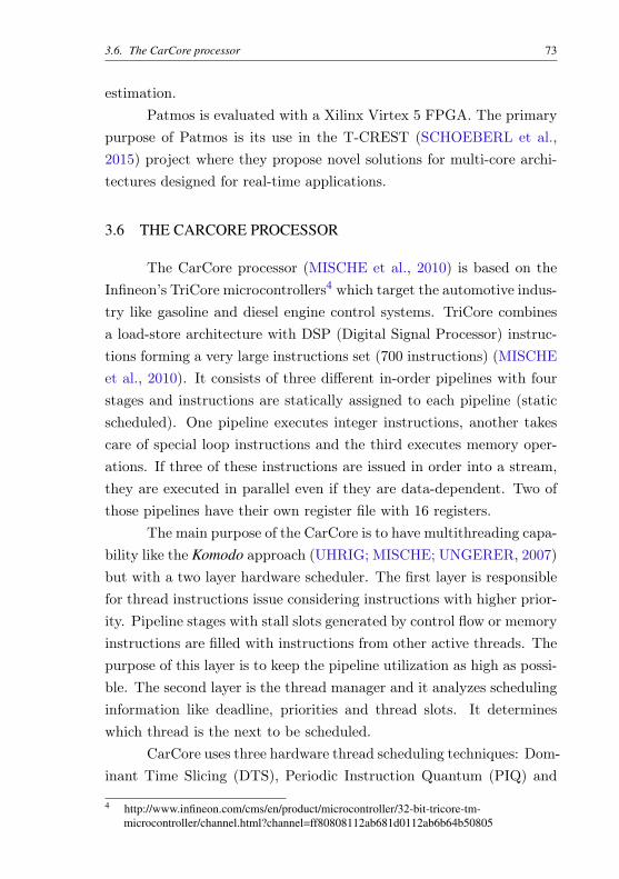
3.6. The CarCore processor 73
estimation.Patmos is evaluated with a Xilinx Virtex 5 FPGA. The primary
purpose of Patmos is its use in the T-CREST (SCHOEBERL et al.,2015) project where they propose novel solutions for multi-core archi-tectures designed for real-time applications.
3.6 THE CARCORE PROCESSOR
The CarCore processor (MISCHE et al., 2010) is based on theInfineon’s TriCore microcontrollers4 which target the automotive indus-try like gasoline and diesel engine control systems. TriCore combinesa load-store architecture with DSP (Digital Signal Processor) instruc-tions forming a very large instructions set (700 instructions) (MISCHEet al., 2010). It consists of three different in-order pipelines with fourstages and instructions are statically assigned to each pipeline (staticscheduled). One pipeline executes integer instructions, another takescare of special loop instructions and the third executes memory oper-ations. If three of these instructions are issued in order into a stream,they are executed in parallel even if they are data-dependent. Two ofthose pipelines have their own register file with 16 registers.
The main purpose of the CarCore is to have multithreading capa-bility like the Komodo approach (UHRIG; MISCHE; UNGERER, 2007)but with a two layer hardware scheduler. The first layer is responsiblefor thread instructions issue considering instructions with higher prior-ity. Pipeline stages with stall slots generated by control flow or memoryinstructions are filled with instructions from other active threads. Thepurpose of this layer is to keep the pipeline utilization as high as possi-ble. The second layer is the thread manager and it analyzes schedulinginformation like deadline, priorities and thread slots. It determineswhich thread is the next to be scheduled.
CarCore uses three hardware thread scheduling techniques: Dom-inant Time Slicing (DTS), Periodic Instruction Quantum (PIQ) and
4 http://www.infineon.com/cms/en/product/microcontroller/32-bit-tricore-tm-microcontroller/channel.html?channel=ff80808112ab681d0112ab6b64b50805
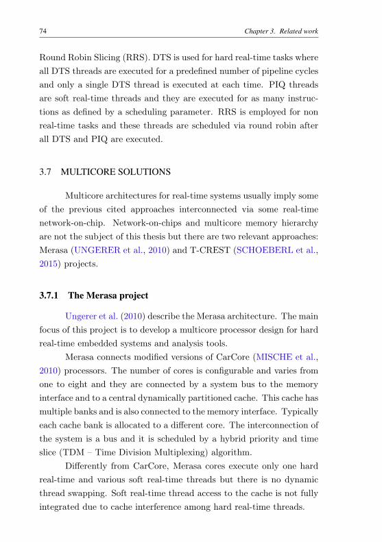
74 Chapter 3. Related work
Round Robin Slicing (RRS). DTS is used for hard real-time tasks whereall DTS threads are executed for a predefined number of pipeline cyclesand only a single DTS thread is executed at each time. PIQ threadsare soft real-time threads and they are executed for as many instruc-tions as defined by a scheduling parameter. RRS is employed for nonreal-time tasks and these threads are scheduled via round robin afterall DTS and PIQ are executed.
3.7 MULTICORE SOLUTIONS
Multicore architectures for real-time systems usually imply someof the previous cited approaches interconnected via some real-timenetwork-on-chip. Network-on-chips and multicore memory hierarchyare not the subject of this thesis but there are two relevant approaches:Merasa (UNGERER et al., 2010) and T-CREST (SCHOEBERL et al.,2015) projects.
3.7.1 The Merasa project
Ungerer et al. (2010) describe the Merasa architecture. The mainfocus of this project is to develop a multicore processor design for hardreal-time embedded systems and analysis tools.
Merasa connects modified versions of CarCore (MISCHE et al.,2010) processors. The number of cores is configurable and varies fromone to eight and they are connected by a system bus to the memoryinterface and to a central dynamically partitioned cache. This cache hasmultiple banks and is also connected to the memory interface. Typicallyeach cache bank is allocated to a different core. The interconnection ofthe system is a bus and it is scheduled by a hybrid priority and timeslice (TDM – Time Division Multiplexing) algorithm.
Differently from CarCore, Merasa cores execute only one hardreal-time and various soft real-time threads but there is no dynamicthread swapping. Soft real-time thread access to the cache is not fullyintegrated due to cache interference among hard real-time threads.
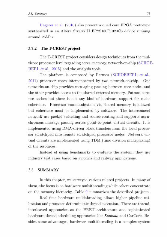
3.8. Summary 75
Ungerer et al. (2010) also present a quad core FPGA prototypesynthesized in an Altera Stratix II EP2S180F1020C3 device runningaround 25Mhz.
3.7.2 The T-CREST project
The T-CREST project considers design techniques from the mul-ticore processor level regarding cores, memory, network-on-chip (SCHOE-BERL et al., 2015) and the analysis tools.
The platform is composed by Patmos (SCHOEBERL et al.,2011) processor cores interconnected by two network-on-chip. Onenetworks-on-chip provides messaging passing between core nodes andthe other provides access to the shared external memory. Patmos coresuse caches but there is not any kind of hardware support for cachecoherence. Processor communication via shared memory is allowedbut coherence must be implemented by software. The interconnectnetwork use packet switching and source routing and supports asyn-chronous message passing across point-to-point virtual circuits. It isimplemented using DMA-driven block transfers from the local proces-sor scratchpad into remote scratchpad processor nodes. Network vir-tual circuits are implemented using TDM (time division multiplexing)of the resources.
Instead of using benchmarks to evaluate the system, they useindustry test cases based on avionics and railway applications.
3.8 SUMMARY
In this chapter, we surveyed various related projects. In many ofthem, the focus is on hardware multithreading while others concentrateon the memory hierarchy. Table 9 summarizes the described projects.
Real-time hardware multithreading allows higher pipeline uti-lization and promotes deterministic thread execution. There are thread-interleaved approaches as the PRET architecture and sophisticatedhardware thread scheduling approaches like Komodo and CarCore. Be-sides some advantages, hardware multithreading is a complex system
76 Chapter 3. Related work
and additional hardware elements like the register file must be repli-cated. Schoeberl (2009b) argues that the additional hardware could beemployed to chip multiprocessing instead of chip multithreading.
Patmos and JOP use a unique cache system where several spe-cialized caches are proposed. It requires effort on the part of softwaredevelopment, but it can enhance the analyzability of the system. Thecompiler must explicitly select memory instructions to access differentcaches and two instructions are required for memory loads.
We can note that all related works have a main objective regard-ing determinism and differently of them, our work is concentrated inthe investigation of a VLIW processor for hard real-time applications.There are many design space investigations and it is not clear how theyimpact on the WCET performance. Among them, we can highlight:pipeline dependencies resolution, full predication for 4-issue VLIW pro-cessor, branch architecture and all of these features are considered inthe WCET analysis tool.
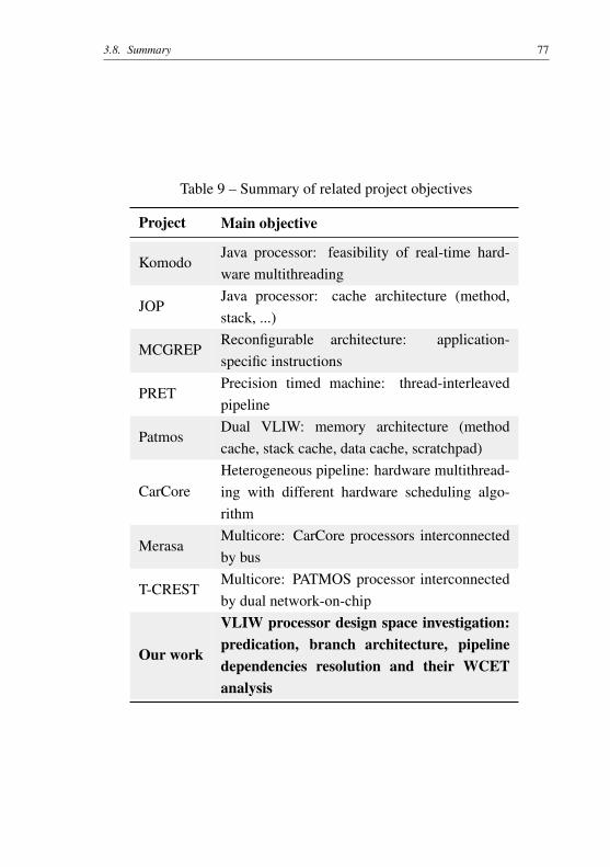
3.8. Summary 77
Table 9 – Summary of related project objectives
Project Main objective
KomodoJava processor: feasibility of real-time hard-ware multithreading
JOPJava processor: cache architecture (method,stack, ...)
MCGREPReconfigurable architecture: application-specific instructions
PRETPrecision timed machine: thread-interleavedpipeline
PatmosDual VLIW: memory architecture (methodcache, stack cache, data cache, scratchpad)
CarCoreHeterogeneous pipeline: hardware multithread-ing with different hardware scheduling algo-rithm
MerasaMulticore: CarCore processors interconnectedby bus
T-CRESTMulticore: PATMOS processor interconnectedby dual network-on-chip
Our work
VLIW processor design space investigation:predication, branch architecture, pipelinedependencies resolution and their WCETanalysis

79
4 THESIS RATIONALE AND DESIGN DECISIONS
The analysis of real-time systems is a challenging task and re-quires the union of numerous techniques. Typically the problem isdivided into two main areas: scheduling analysis and temporal analysisof individual tasks.
Scheduling analysis is responsible for verifying the system fea-sibility as a scheduling problem: we want to verify if a task set canexecute properly respecting the individual deadline of each task.
The formulation of the scheduling problem will always dependon the temporal system parameters. Obtaining these parameters is theresponsibility of the task’s individual temporal analysis. Some of theseparameters are dependent on what we want to control or sample usinga real-time system, like the activation frequency or task period (T ).However, a key parameter is the Worst-Case Execution Time (WCET)of each task – (C). Every scheduling analysis depends on the WCET.The focus of this work is on the temporal analysis of individual tasks,more specifically, on researching deterministic hardware techniques toimprove the WCET analysis but also increase processor performance.
As noted briefly in the previous chapters, in recent years con-siderable research effort has been done on providing time-predictablearchitectures for real-time systems. Since general-purpose processorsusually focus on average-case performance (SCHOEBERL et al., 2015),analyzing real-time systems and obtaining WCET using those proces-sors became very complex. Real-time applications are becoming in-creasingly more complex requiring more processing power with em-bedded systems providing more and more “desktop-like” functionality.However, the use of standard processor design choices to improve per-formance is usually not possible for real-time systems because it greatlyjeopardizes determinism proprieties.
In this chapter, we describe the target problem and the thesisrationale. We will present the target systems, their requirements anddiscuss design decisions for the proposed architecture comparing themwith the related researches.
80 Chapter 4. Thesis rationale and design decisions
4.1 TARGET SYSTEMS AND REQUIREMENTS
Currently the use of microprocessors is ubiquitous. They arewidely embedded in general consumer goods (cameras, TVs, videogameconsoles, robots), automotive market (navigation, vision), aviation andcommunication (cell phones, routers). Another market for microproces-sors is the personal computer (PC) as the main processor. Because ofthe versatility of a PC, its processor is usually called a general-purposeprocessor and the user can reprogram it and extend its functionalitywith new software using complex and big applications. In the case ofembedded computing systems, they are encapsulated in a device andgenerally are not intended to reprogramming by the user. Moreover,embedded processors, which are the focus of this work, must complywith various non-functional requirements:
∙ Instead of running functions as quickly as possible, embeddedapplications often must respect the real-time requirements (com-pliance with deadlines).
∙ Embedded devices, especially powered by batteries, have energyrestrictions.
∙ Instead of binary compatibility, source compatibility is more im-portant.
Safety standards for embedded applications (DO-178B, DO-178C,IEC-61508, ISO-26262, EN-50125, etc.) require identifying potentialfunctional and non-functional hazards and we must demonstrate thatthe software complies with safety goals. Testing with intensive mea-surements is tedious and also typically not safe. It is often impossibleto prove that the worst-case conditions have actually been taken intoaccount. As DO-178B succinctly puts it, “testing, in general, cannotshow the absence of errors”.
Despite the differences between general purpose and embeddedcomputing, the addition of new functionality such as audio/video pro-cessing, networking, security, automation and control, among others,
4.2. Thesis Objective 81
increases the need for more advanced processors for embedded appli-cations. However, deterministic hardware is necessary when the appli-cation has hard real-time requirements.
In terms of target systems and requirements, we will focus:
∙ Target systems: embedded systems.
∙ Low-level requirements: hard real-time. The proposed designmust be time predictable allowing safe and precise WCET estima-tions. We must design techniques to obtain worst-case behaviorand timing of every used hardware component.
∙ High-level requirements: the architecture should use an ISA –Instruction Set Architecture – that allows the use of a modernC compiler. It should provide clear and well defined instructionencoding, adequate set of arithmetic instructions, typical memoryaccess instruction with base plus offset addressing mode and allowthe use of function calling/returning.
4.2 THESIS OBJECTIVE
The general objective of this thesis is to investigate various pro-cessor architecture features that lead to predictable designs with rea-sonable WCET performance. The thesis to be demonstrated is that itis possible to assemble together hardware elements that increase per-formance but are predictable enough to ensure precise and efficienttemporal analyses. In order to improve them, especially the worst-caseexecution time analysis, the design of processors should increase thelevel of importance of the determinism.
Therefore, it is necessary to analyze the strengths of hardwaretechniques used in state-of-the-art processors, for example temporaland spatial parallelism (pipeline), branch prediction and predication,and to align them to real-time applications. Some of these techniquesrequire modifications due to high hardware complexity while othersneed a well-defined timing behavior. In order to achieve these goals,
82 Chapter 4. Thesis rationale and design decisions
we propose new approaches considering the following items which aredescribed in the next sections:
∙ Target architecture definition: based on the predictability con-siderations, what is a good target architecture model?
∙ Predication: how predication could be improved without jeopar-dizing pipeline performance due to overheads in the encoding anddata paths?
∙ Branch prediction: how much performance is gained by usingbranch prediction? How we define its timing behavior?
∙ Pipeline dependencies: which are the main sources of dependen-cies and how to deal with them?
∙ High latency operations: how much performance is lost with highlatency operations like memory access, multiplication and divi-sion? How to deal with it?
Besides the approaches exposed above, one of the most impor-tant tasks of this thesis is to propose a WCET analysis for the pro-posed architecture. This analyzer and Mälardalen WCET benchmarks(GUSTAFSSON et al., 2010) are used to make evaluations regardingdeterminism and performance.
4.3 ARCHITECTURE
After having laid the ground work for predictability considera-tions of processors, related research, our target class of system and itsrequirements, we noticed that there are basically two main approachesfor real-time computer architectures: chip multithreading and VLIW– Very Long Instruction Word processors, since superscalabilty andout-of-order execution are not adequate.
Chip multithreading permits several threads to share pipeline re-sources possibly increasing performance and pipeline utilization. How-ever, it requires some critical components (such as the register file) to
4.3. Architecture 83
be replicated for the number of threads because the hardware needsdifferent execution contexts. Multithreading as a thread interleavedpipeline (used in PRET) could also remove data dependencies betweenpipeline stages because in each different pipeline stage there is a differ-ent thread executing. Using this technique, in (LIU et al., 2012), it isargued that they do not use forwarding logic and use round-robin forfine-grained thread scheduling. If there is no forwarding logic betweenstages and less than 4 threads, some sort of stalling should occur. Onthe other hand, the use of round-robin thread scheduling impacts theresponse time of the task set: fetching the next instruction for a threadmust wait the fetch for all other threads, i.e., if we have 4 threads anda pipeline with 4 stages, after 4 cycles another instruction is fetchedfor a particular thread.
In contrast to chip multithreading, VLIW machines increasesingle-threading performance where instructions are executed in thepipeline in temporal and spatial parallelism, i.e., more than one oper-ation in each pipeline stage. To do so, execution units like arithmeticunits are replicated, being this a common practice in state-of-the-artprocessors. Differently from those processors, VLIW instructions arestatically scheduled during compilation, which is very interesting be-cause it is defined offline and does not depend on hardware fetch states.VLIW typically uses less power comparing to superscalar out-of-orderdesigns since less hardware is required for instruction scheduling. Com-pared to PRET, VLIW also needs forwarding logic and, with moreparallel execution units, this forwarding logic becomes more complex.But according to (FISHER; FARABOSHI; YOUNG, 2005), 4-issue for-warding logic is perfectly feasible, even in soft-core implementations.As noted before, in (SCHOEBERL et al., 2011) they presented a VLIWdual-fetch processor optimized for real-time applications named Pat-mos. Compared to state-of-the-art and commercial VLIW processors,Patmos is relatively simple: dual issue and five stage pipeline. The ma-jor difference of Patmos is its memory architecture, which has differentcache memories for each segment: stack, heap, instruction, etc. Ac-cess to different data caches in Patmos uses different ISA instructions.
84 Chapter 4. Thesis rationale and design decisions
The use of different caches for different kinds of data could simplifythe WCET analysis. However, the programming model is also affected,particularly the compiler if there are distinct memory instructions touse. Patmos also supports fully predicated instructions to promote thesingle-path programming paradigm (PUSCHNER, 2005).
A comparison between single and multithreading is not the pur-pose of this thesis, since both have suitable applications. Our focus isplaced on the VLIW approach. The research of real-time computer ar-chitectures is challenging and involves many aspects, not all problemswere resolved by recent published papers and, to continue research-ing, a customizable platform is necessary. Besides being predictable, areal-time processor should have a reasonable worst-case performance.State-of-the-art processors are superscalar since they fetch and executemore than one instruction per cycle. VLIW could be used to do so ina real-time platform.
Our first contribution to the state of the art is the investigationof the design space of VLIW processors for hard real-time applications.It is already known that VLIW approaches are more adequate for real-time applications but static instruction scheduling alone is not enoughto guarantee determinism. VLIW requires some sort of instruction en-coding since parallel operations are scheduled together by the compiler.Instruction encoding could be as simple as adding nops to empty op-erations slots or as complex as CISC encoding with variable operationdelimitation. The use of a simple encoding jeopardizes performancesince it adds instruction memory overhead and a complex encodingjeopardizes determinism since pre-fetch buffers could be necessary inthe pipeline front-end. There are many other design space investiga-tions and they will be described in the following sections. We can alsohighlight: pipeline dependencies resolution, full predication for 4-issueVLIW processors, branch architecture and the first level of the memorysubsystem.
We can also note that the only recent work that directly appliesVLIW for real-time systems is Patmos. Its primary focus is the memoryarchitecture and it was used later in the T-CREST multi-core project.
4.4. Design decisions 85
The WCET estimation of Patmos is not clearly described since it uses aprototype of aiT 1 proprietary software. We make a second contributionsince every hardware aspect we used in the processor is clearly describedin the WCET analysis tool.
4.4 DESIGN DECISIONS
After we defined VLIW as the target architecture, this sectiondescribes our new approaches and answer the questions raised earlier.We also consider important decisions like Instruction Set Architecture(ISA), instruction encoding, compiler and memory architecture, sincea processor can not work without them.
4.4.1 Instruction set and encoding
We adopted a subset of the HP VLIW ST231 instruction set withcustomized special instructions. By using this instruction set, we relyon a vast VLIW documentation, a compiler and cycle accurate simula-tor. This documentation and tools are presented in Fisher, Faraboshiand Young (2005) covering the VLIW architecture in a way similar toPatterson and Hennessy (2007) covering the MIPS architecture. Bothcompiler and simulator are called VEX – VLIW EXample 2. They areproprietary and their source code is not available but we can use themas a baseline since the VLIW approach of these tools does not considerreal-time aspects and WCET analysis. The VEX compiler is based onthe Multiflow C compiler with global trace instruction scheduling andit is highly optimized for VLIW processors.
4.4.1.1 Instruction bundle encoding
In a VLIW machine, an instruction or instruction bundle is com-prised of operations or syllables. Considering a 4-issue fetch unit, aninstruction can be composed of one, two, three, four operations or many
1 http://www.absint.com/ait/2 http://www.hpl.hp.com/downloads/vex/
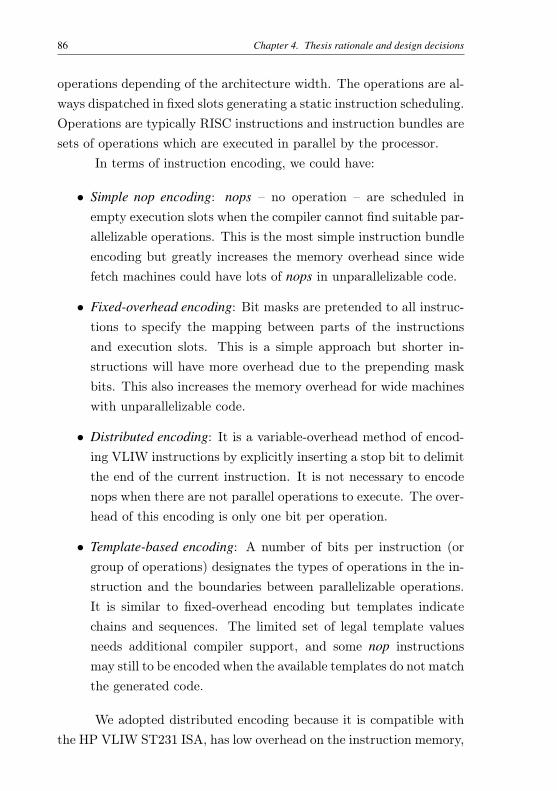
86 Chapter 4. Thesis rationale and design decisions
operations depending of the architecture width. The operations are al-ways dispatched in fixed slots generating a static instruction scheduling.Operations are typically RISC instructions and instruction bundles aresets of operations which are executed in parallel by the processor.
In terms of instruction encoding, we could have:
∙ Simple nop encoding: nops – no operation – are scheduled inempty execution slots when the compiler cannot find suitable par-allelizable operations. This is the most simple instruction bundleencoding but greatly increases the memory overhead since widefetch machines could have lots of nops in unparallelizable code.
∙ Fixed-overhead encoding: Bit masks are pretended to all instruc-tions to specify the mapping between parts of the instructionsand execution slots. This is a simple approach but shorter in-structions will have more overhead due to the prepending maskbits. This also increases the memory overhead for wide machineswith unparallelizable code.
∙ Distributed encoding: It is a variable-overhead method of encod-ing VLIW instructions by explicitly inserting a stop bit to delimitthe end of the current instruction. It is not necessary to encodenops when there are not parallel operations to execute. The over-head of this encoding is only one bit per operation.
∙ Template-based encoding: A number of bits per instruction (orgroup of operations) designates the types of operations in the in-struction and the boundaries between parallelizable operations.It is similar to fixed-overhead encoding but templates indicatechains and sequences. The limited set of legal template valuesneeds additional compiler support, and some nop instructionsmay still to be encoded when the available templates do not matchthe generated code.
We adopted distributed encoding because it is compatible withthe HP VLIW ST231 ISA, has low overhead on the instruction memory,
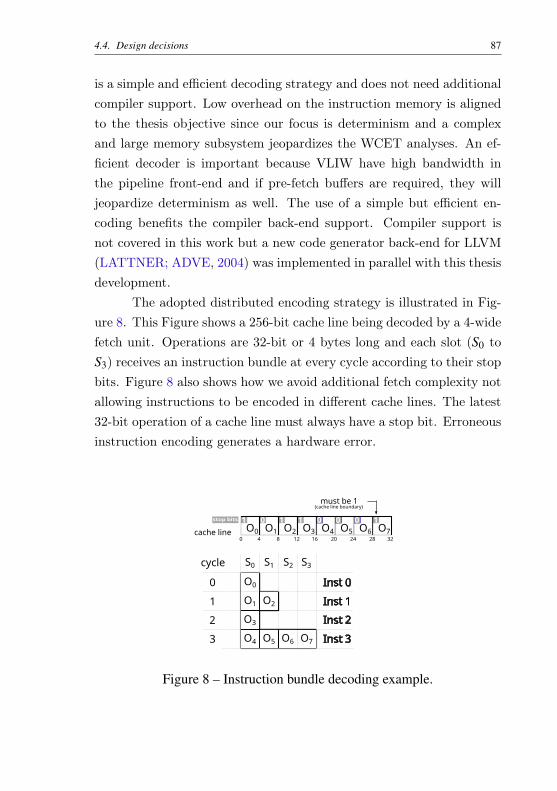
4.4. Design decisions 87
is a simple and efficient decoding strategy and does not need additionalcompiler support. Low overhead on the instruction memory is alignedto the thesis objective since our focus is determinism and a complexand large memory subsystem jeopardizes the WCET analyses. An ef-ficient decoder is important because VLIW have high bandwidth inthe pipeline front-end and if pre-fetch buffers are required, they willjeopardize determinism as well. The use of a simple but efficient en-coding benefits the compiler back-end support. Compiler support isnot covered in this work but a new code generator back-end for LLVM(LATTNER; ADVE, 2004) was implemented in parallel with this thesisdevelopment.
The adopted distributed encoding strategy is illustrated in Fig-ure 8. This Figure shows a 256-bit cache line being decoded by a 4-widefetch unit. Operations are 32-bit or 4 bytes long and each slot (S0 toS3) receives an instruction bundle at every cycle according to their stopbits. Figure 8 also shows how we avoid additional fetch complexity notallowing instructions to be encoded in different cache lines. The latest32-bit operation of a cache line must always have a stop bit. Erroneousinstruction encoding generates a hardware error.
O01
cache line
must be 1
O10
O21
O31
O71
O40
O50
O600 0 00 0 00 0 0
40 8 12 16 20 24 28 32
stop bits
(cache line boundary)
O7O4 O6O5
O3
O1 O2
O0
cycle
0
1
2
3
S1 S2 S3
Inst 0
Inst 1
Inst 2
Inst 3
S0
Figure 8 – Instruction bundle decoding example.
88 Chapter 4. Thesis rationale and design decisions
4.4.1.2 Operation encoding
Table 10 presents a summary of the VLIW ST231 ISA operationencoding. The encoding is well defined: the format field is used toidentify different classes between integer, special, memory or controlflow operations. The special class is used for selecting instructions andother special instructions like break point and long immediates. Theopcode field specifies the operation type considering the format classes.Bits 20..12 are assigned to short immediate, destination or operand 2registers depending on the operation format and opcode. Bits 11..6 areassigned to operand 2 or destination registers and it also depends onthe format and opcode. Bits 5..0 are only assigned to register operand1. More details of the operation encoding can be found in the ST231Core and Instruction Set Architecture Manual 3.
Table 10 – Operation encoding.
Bits Function Description
31 Stop bit Determines bundle ending
30 Full-predicationNot supported by ST-231, used forfull predication extension
29..28 FormatOperation Format: integer, special,memory or control flow classes
27..21 Opcode Operation opcode within format class
20..12 Immediate/dest/src2Short immediate, destination registeror operand 2 register
11..6 dest/scr2 Register operand 2 or destination5..0 src1 Register operand 1
The VLIW ST231 ISA supports only partial predication: thehardware supports select instructions in which one value is selectedbetween two input parameters and one binary selector (predicate). Webelieve that partial predication alone generates too much instruction
3 http://lipforge.ens-lyon.fr/docman/view.php/53/26/st231arch.pdf
4.4. Design decisions 89
memory and compiler overhead. We extended predication capabilitiesadding full predication support where blocks of instructions can beturned off. This feature will be described in Section 4.4.3.
Like the ST231 ISA, we support 9-bit immediate data (encodedin a single operation) or long 32-bit immediate data (using 64-bit).Long immediates can be on the left or right of an arithmetic operationusing the special long immediate operation.
Branches and jumps use a 23-bit PC (Program Counter) offset.The integer offset is encoded using bits 22..0 when using the control-flowinstruction format. Function calls to 32-bit addresses are supported bya register indirect branch and link instruction.
There is a complete set of compare instructions and they areflexible: the destination can be a predicate or a general purpose registerand the source can be only register or register/immediate. A total of64 32-bit registers could be encoded ($r) and 8 1-bit predicates ($br).The number of predicates can only be increased using a clustered designbecause there are no available encoding bits. The complete operationlist is available in Appendix A.
4.4.2 Processor pipeline
We propose a VLIW design featuring with full forwarded exe-cution stage units to prevent additional stalls from Read after Write(RAW) data dependencies. It means that any calculation performedby any unit is forwarded to the unit which needs the data. Figure 9shows an overview of the adopted pipeline design. Forwarding logicdata paths and the register file are omitted. The black arrows indicatethe data path between the pipeline stages and the execution units. A64 32-bit register file and a 8 1-bit predicate register file are commonto all execution units.
Our design has 5 stages:
∙ “F” – Cache Buffer: This stage is connected directly to the cacheinstruction memory and it represents the pipeline front-end. Itcontrols the cache memory providing its address and receives stall
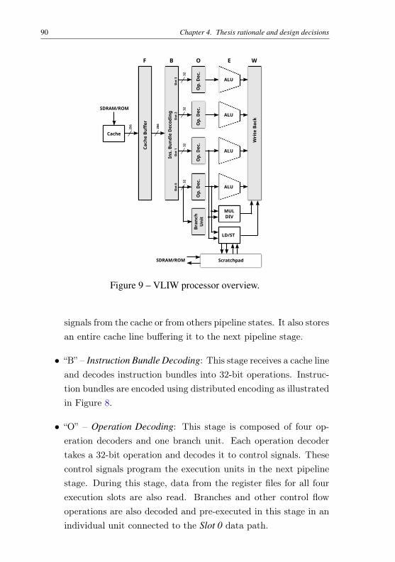
90 Chapter 4. Thesis rationale and design decisions
Wri
te B
ack
Ins.
Bun
dle
Dec
odin
g
ALU
ALU
ALU
ALU
Op.
Dec
.
LD/ST
MULDIV
Bran
chU
nit
Slot
0Sl
ot 1
Slot
2Sl
ot 3
256
256
3232
3232
Cach
e Bu
ffer
Op.
Dec
.O
p. D
ec.
Op.
Dec
.
F B O E W
Cache
CacheScratchpad
SDRAM/ROM
SDRAM/ROM
Figure 9 – VLIW processor overview.
signals from the cache or from others pipeline states. It also storesan entire cache line buffering it to the next pipeline stage.
∙ “B” – Instruction Bundle Decoding: This stage receives a cache lineand decodes instruction bundles into 32-bit operations. Instruc-tion bundles are encoded using distributed encoding as illustratedin Figure 8.
∙ “O” – Operation Decoding: This stage is composed of four op-eration decoders and one branch unit. Each operation decodertakes a 32-bit operation and decodes it to control signals. Thesecontrol signals program the execution units in the next pipelinestage. During this stage, data from the register files for all fourexecution slots are also read. Branches and other control flowoperations are also decoded and pre-executed in this stage in anindividual unit connected to the Slot 0 data path.
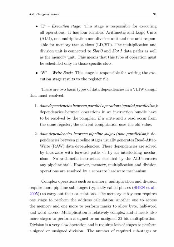
4.4. Design decisions 91
∙ “E” – Execution stage: This stage is responsible for executingall operations. It has four identical Arithmetic and Logic Units(ALU), one multiplication and division unit and one unit respon-sible for memory transactions (LD/ST). The multiplication anddivision unit is connected to Slot 0 and Slot 1 data paths as wellas the memory unit. This means that this type of operation mustbe scheduled only in those specific slots.
∙ “W” – Write Back: This stage is responsible for writing the exe-cution stage results to the register file.
There are two basic types of data dependencies in a VLIW designthat must resolved:
1. data dependencies between parallel operations (spatial parallelism):dependencies between operations in an instruction bundle haveto be resolved by the compiler: if a write and a read occur fromthe same register, the current computation uses the old value.
2. data dependencies between pipeline stages (time parallelism): de-pendencies between pipeline stages usually generates Read-After-Write (RAW) data dependencies. These dependencies are solvedby hardware with forward paths or by an interlocking mecha-nism. No arithmetic instruction executed by the ALUs causesany pipeline stall. However, memory, multiplication and divisionoperations are resolved by a separate hardware mechanism.
Complex operations such as memory, multiplication and divisionrequire more pipeline sub-stages (typically called phases (SHEN et al.,2005)) to carry out their calculations. The memory subsystem requiresone stage to perform the address calculation, another one to accessthe memory and one more to perform masks to allow byte, half-wordand word access. Multiplication is relatively complex and it needs alsomore stages to perform a signed or an unsigned 32-bit multiplication.Division is a very slow operation and it requires lots of stages to performa signed or unsigned division. The number of required sub-stages or
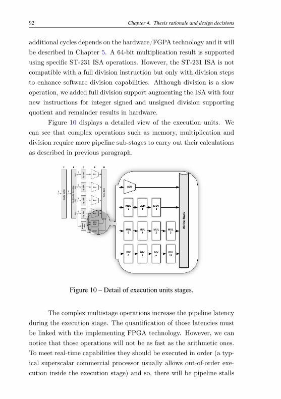
92 Chapter 4. Thesis rationale and design decisions
additional cycles depends on the hardware/FGPA technology and it willbe described in Chapter 5. A 64-bit multiplication result is supportedusing specific ST-231 ISA operations. However, the ST-231 ISA is notcompatible with a full division instruction but only with division stepsto enhance software division capabilities. Although division is a slowoperation, we added full division support augmenting the ISA with fournew instructions for integer signed and unsigned division supportingquotient and remainder results in hardware.
Figure 10 displays a detailed view of the execution units. Wecan see that complex operations such as memory, multiplication anddivision require more pipeline sub-stages to carry out their calculationsas described in previous paragraph.
Wri
te B
ack
Ins.
Bun
dle
Dec
odin
g
ALU
ALU
ALU
ALU
Op.
Dec
.
LD/ST
MULDIV
Bran
chU
nit
Slot
0Sl
ot 1
Slot
2Sl
ot 3
256
256
3232
3232
Cach
e Bu
ffer
Op.
Dec
.O
p. D
ec.
Op.
Dec
.
F B O E W
ALUW
rite
Bac
k
MUL0
MUL1
MUL2
DIV0
DIV1
DIVn
DIV19
MUL3
Figure 10 – Detail of execution units stages.
The complex multistage operations increase the pipeline latencyduring the execution stage. The quantification of those latencies mustbe linked with the implementing FPGA technology. However, we cannotice that those operations will not be as fast as the arithmetic ones.To meet real-time capabilities they should be executed in order (a typ-ical superscalar commercial processor usually allows out-of-order exe-cution inside the execution stage) and so, there will be pipeline stalls
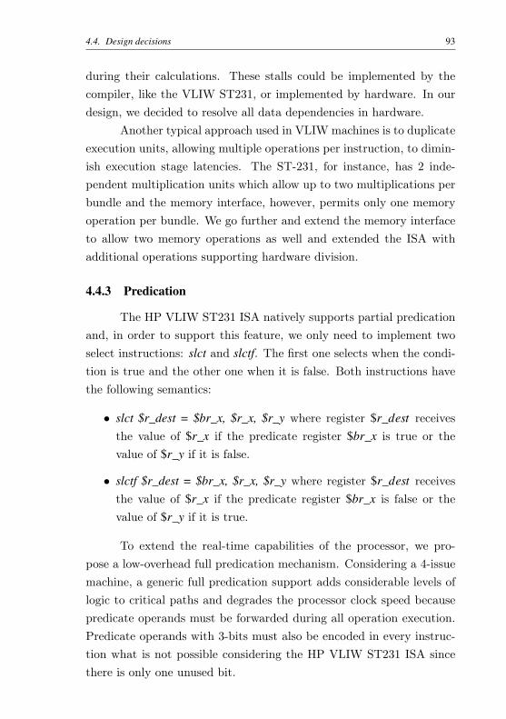
4.4. Design decisions 93
during their calculations. These stalls could be implemented by thecompiler, like the VLIW ST231, or implemented by hardware. In ourdesign, we decided to resolve all data dependencies in hardware.
Another typical approach used in VLIW machines is to duplicateexecution units, allowing multiple operations per instruction, to dimin-ish execution stage latencies. The ST-231, for instance, has 2 inde-pendent multiplication units which allow up to two multiplications perbundle and the memory interface, however, permits only one memoryoperation per bundle. We go further and extend the memory interfaceto allow two memory operations as well and extended the ISA withadditional operations supporting hardware division.
4.4.3 Predication
The HP VLIW ST231 ISA natively supports partial predicationand, in order to support this feature, we only need to implement twoselect instructions: slct and slctf. The first one selects when the condi-tion is true and the other one when it is false. Both instructions havethe following semantics:
∙ slct $r_dest = $br_x, $r_x, $r_y where register $r_dest receivesthe value of $r_x if the predicate register $br_x is true or thevalue of $r_y if it is false.
∙ slctf $r_dest = $br_x, $r_x, $r_y where register $r_dest receivesthe value of $r_x if the predicate register $br_x is false or thevalue of $r_y if it is true.
To extend the real-time capabilities of the processor, we pro-pose a low-overhead full predication mechanism. Considering a 4-issuemachine, a generic full predication support adds considerable levels oflogic to critical paths and degrades the processor clock speed becausepredicate operands must be forwarded during all operation execution.Predicate operands with 3-bits must also be encoded in every instruc-tion what is not possible considering the HP VLIW ST231 ISA sincethere is only one unused bit.
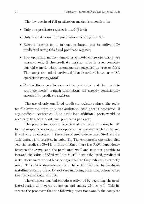
94 Chapter 4. Thesis rationale and design decisions
The low overhead full predication mechanism consists in:
∙ Only one predicate register is used ($br4);
∙ Only one bit is used for predication encoding (bit 30);
∙ Every operation in an instruction bundle can be individuallypredicated using this fixed predicate register;
∙ Two operating modes: simple true mode where operations areexecuted only if the predicate register value is true; completetrue/false mode where operations are executed on true or false.The complete mode is activated/deactivated with two new ISAoperations paron/paroff ;
∙ Control flow operations cannot be predicated and they reset tocomplete mode. Branch instructions are already conditionallyexecuted by predicate registers.
The use of only one fixed predicate register reduces the regis-ter file overhead since only one additional read port is necessary. Ifany predicate register could be used, four additional ports would benecessary to read 4 additional predicates per cycle.
The predication system is activated primarily on using bit 30.In the simple true mode, if an operation is encoded with bit 30 set,it will only be executed if the value of predicate register $br4 is true.This feature is illustrated in Table 11. The comparison operation thatsets the predicate $br4 is in Line 4. Since there is a RAW dependencybetween the cmpgt and the predicated mull and it is not possible toforward the value of $br4 while it is still been calculated, predicatedinstructions must wait at least one cycle before the predicate is correctlyread. This RAW dependency could be either resolved by hardwareinstalling a stall cycle or by software including other instruction beforethe predicated code snippet.
The complete true/false mode is activated by beginning the pred-icated region with paron operation and ending with paroff. This in-structs the processor that the following operations are in the complete
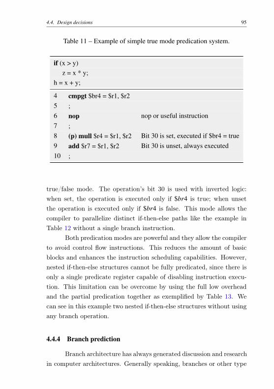
4.4. Design decisions 95
Table 11 – Example of simple true mode predication system.
if (x > y)z = x * y;
h = x + y;
4 cmpgt $br4 = $r1, $r25 ;6 nop nop or useful instruction7 ;8 (p) mull $r4 = $r1, $r2 Bit 30 is set, executed if $br4 = true9 add $r7 = $r1, $r2 Bit 30 is unset, always executed10 ;
true/false mode. The operation’s bit 30 is used with inverted logic:when set, the operation is executed only if $br4 is true; when unsetthe operation is executed only if $br4 is false. This mode allows thecompiler to parallelize distinct if-then-else paths like the example inTable 12 without a single branch instruction.
Both predication modes are powerful and they allow the compilerto avoid control flow instructions. This reduces the amount of basicblocks and enhances the instruction scheduling capabilities. However,nested if-then-else structures cannot be fully predicated, since there isonly a single predicate register capable of disabling instruction execu-tion. This limitation can be overcome by using the full low overheadand the partial predication together as exemplified by Table 13. Wecan see in this example two nested if-then-else structures without usingany branch operation.
4.4.4 Branch prediction
Branch architecture has always generated discussion and researchin computer architectures. Generally speaking, branches or other type
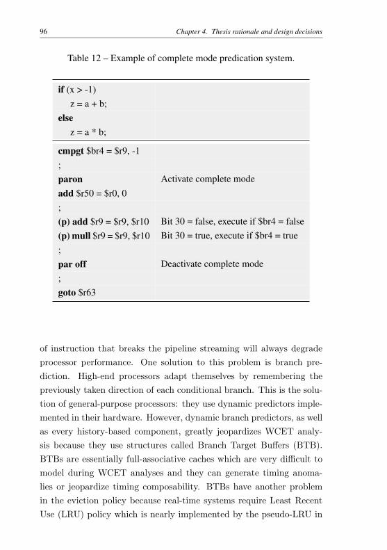
96 Chapter 4. Thesis rationale and design decisions
Table 12 – Example of complete mode predication system.
if (x > -1)z = a + b;
elsez = a * b;
cmpgt $br4 = $r9, -1;paron Activate complete modeadd $r50 = $r0, 0;(p) add $r9 = $r9, $r10 Bit 30 = false, execute if $br4 = false(p) mull $r9 = $r9, $r10 Bit 30 = true, execute if $br4 = true;par off Deactivate complete mode;goto $r63
of instruction that breaks the pipeline streaming will always degradeprocessor performance. One solution to this problem is branch pre-diction. High-end processors adapt themselves by remembering thepreviously taken direction of each conditional branch. This is the solu-tion of general-purpose processors: they use dynamic predictors imple-mented in their hardware. However, dynamic branch predictors, as wellas every history-based component, greatly jeopardizes WCET analy-sis because they use structures called Branch Target Buffers (BTB).BTBs are essentially full-associative caches which are very difficult tomodel during WCET analyses and they can generate timing anoma-lies or jeopardize timing composability. BTBs have another problemin the eviction policy because real-time systems require Least RecentUse (LRU) policy which is nearly implemented by the pseudo-LRU in
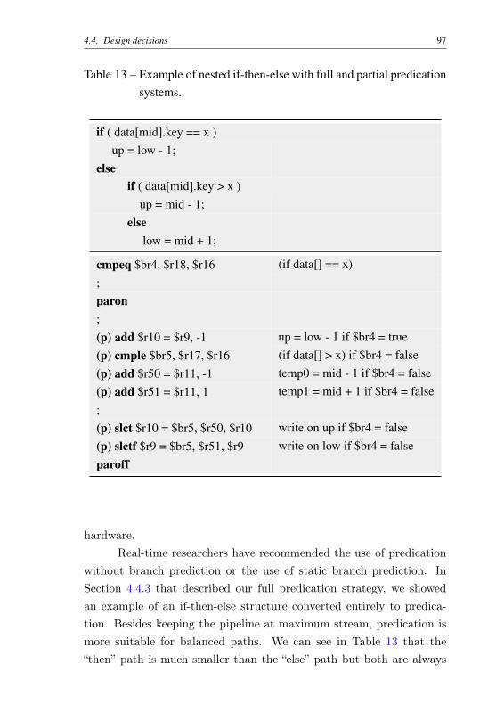
4.4. Design decisions 97
Table 13 – Example of nested if-then-else with full and partial predicationsystems.
if ( data[mid].key == x )up = low - 1;
elseif ( data[mid].key > x )
up = mid - 1;else
low = mid + 1;
cmpeq $br4, $r18, $r16 (if data[] == x);paron;(p) add $r10 = $r9, -1 up = low - 1 if $br4 = true(p) cmple $br5, $r17, $r16 (if data[] > x) if $br4 = false(p) add $r50 = $r11, -1 temp0 = mid - 1 if $br4 = false(p) add $r51 = $r11, 1 temp1 = mid + 1 if $br4 = false;(p) slct $r10 = $br5, $r50, $r10 write on up if $br4 = false(p) slctf $r9 = $br5, $r51, $r9 write on low if $br4 = falseparoff
hardware.Real-time researchers have recommended the use of predication
without branch prediction or the use of static branch prediction. InSection 4.4.3 that described our full predication strategy, we showedan example of an if-then-else structure converted entirely to predica-tion. Besides keeping the pipeline at maximum stream, predication ismore suitable for balanced paths. We can see in Table 13 that the“then” path is much smaller than the “else” path but both are always
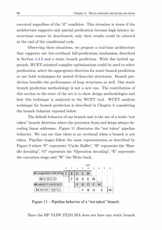
98 Chapter 4. Thesis rationale and design decisions
executed regardless of the “if” condition. This situation is worse if thearchitecture supports only partial predication because high latency in-structions cannot be deactivated, only their results could be selectedat the end of the conditional code.
Observing these situations, we propose a real-time architecturethat supports our low-overhead full-predication mechanism describedin Section 4.4.3 and a static branch prediction. With this hybrid ap-proach, WCET-oriented compiler optimizations could be used to selectpredication, select the appropriate direction for static branch predictionor use both techniques for nested if-then-else structures. Branch pre-diction benefits the performance of loop structures as well. Our staticbranch prediction methodology is not a new one. The contribution ofthis section to the state of the art is to show design methodologies andhow this technique is analyzed in the WCET tool. WCET analysistechnique for branch prediction is described in Chapter 6 consideringthe branch behavior exposed below.
The default behavior of our branch unit is the use of a static “nottaken” branch direction where the processor front-end keeps always de-coding linear addresses. Figure 11 illustrates the “not taken” pipelinebehavior. We can see that there is no overhead when a branch is nottaken. Pipeline stages follow the same representation as described byFigure 9 where “F” represents “Cache Buffer”, “B” represents the “Bun-dle decoding”, “O” represents the “Operation decoding”, “E” representsthe execution stage and “W” the Write back.
cycle
61: cmpgt $br0 = $r9, $r10
62: br $br0, 26
63: add $r11 = $r10, $r11
64: ldw $r8 = 16[$r12]
0 1 2 3 4 5 6 7 8
Figure 11 – Pipeline behavior of a “not taken” branch.
Since the HP VLIW ST231 ISA does not have any static branch
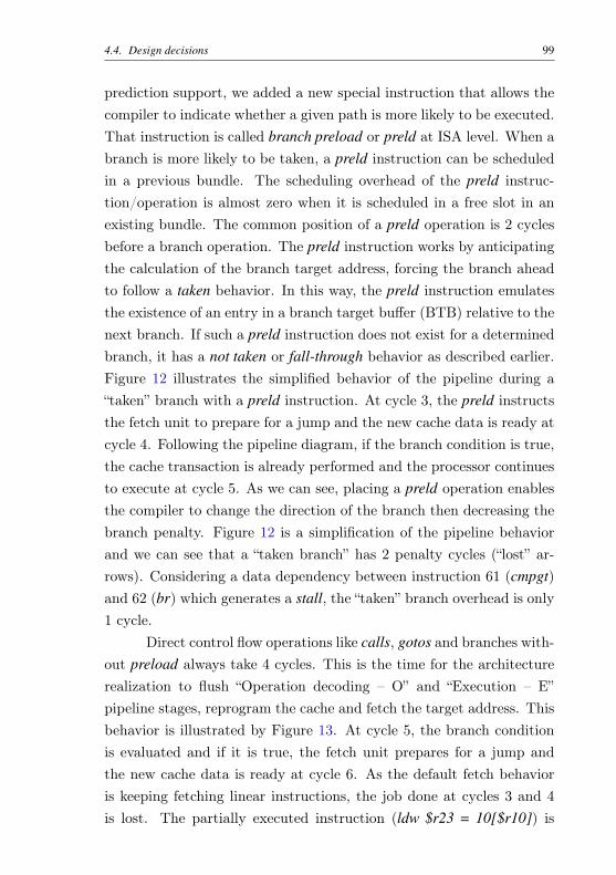
4.4. Design decisions 99
prediction support, we added a new special instruction that allows thecompiler to indicate whether a given path is more likely to be executed.That instruction is called branch preload or preld at ISA level. When abranch is more likely to be taken, a preld instruction can be scheduledin a previous bundle. The scheduling overhead of the preld instruc-tion/operation is almost zero when it is scheduled in a free slot in anexisting bundle. The common position of a preld operation is 2 cyclesbefore a branch operation. The preld instruction works by anticipatingthe calculation of the branch target address, forcing the branch aheadto follow a taken behavior. In this way, the preld instruction emulatesthe existence of an entry in a branch target buffer (BTB) relative to thenext branch. If such a preld instruction does not exist for a determinedbranch, it has a not taken or fall-through behavior as described earlier.Figure 12 illustrates the simplified behavior of the pipeline during a“taken” branch with a preld instruction. At cycle 3, the preld instructsthe fetch unit to prepare for a jump and the new cache data is ready atcycle 4. Following the pipeline diagram, if the branch condition is true,the cache transaction is already performed and the processor continuesto execute at cycle 5. As we can see, placing a preld operation enablesthe compiler to change the direction of the branch then decreasing thebranch penalty. Figure 12 is a simplification of the pipeline behaviorand we can see that a “taken branch” has 2 penalty cycles (“lost” ar-rows). Considering a data dependency between instruction 61 (cmpgt)and 62 (br) which generates a stall, the “taken” branch overhead is only1 cycle.
Direct control flow operations like calls, gotos and branches with-out preload always take 4 cycles. This is the time for the architecturerealization to flush “Operation decoding – O” and “Execution – E”pipeline stages, reprogram the cache and fetch the target address. Thisbehavior is illustrated by Figure 13. At cycle 5, the branch conditionis evaluated and if it is true, the fetch unit prepares for a jump andthe new cache data is ready at cycle 6. As the default fetch behavioris keeping fetching linear instructions, the job done at cycles 3 and 4is lost. The partially executed instruction (ldw $r23 = 10[$r10]) is
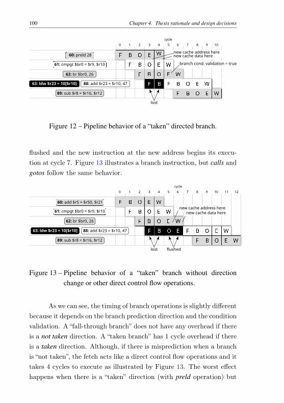
100 Chapter 4. Thesis rationale and design decisions
cycle
61: cmpgt $br0 = $r9, $r10
62: br $br0, 26
89: sub $r8 = $r16, $r12
60: preld 28
0 1 2 3 4 5 6 7 8 9 10
branch cond. validation = true
new cache address here
88: add $r23 = $r10, 4763: ldw $r23 = 10[$r10]
lost
new cache data here
Figure 12 – Pipeline behavior of a “taken” directed branch.
flushed and the new instruction at the new address begins its execu-tion at cycle 7. Figure 13 illustrates a branch instruction, but calls andgotos follow the same behavior.
cycle
61: cmpgt $br0 = $r9, $r10
62: br $br0, 26
89: sub $r8 = $r16, $r12
60: add $r5 = $r50, $r21
0 1 2 3 4 5 6 7 8 9 10 11 12
new cache address herenew cache data here
88: add $r23 = $r10, 4763: ldw $r23 = 10[$r10]
lost flushed
Figure 13 – Pipeline behavior of a “taken” branch without directionchange or other direct control flow operations.
As we can see, the timing of branch operations is slightly differentbecause it depends on the branch prediction direction and the conditionvalidation. A “fall-through branch” does not have any overhead if thereis a not taken direction. A “taken branch” has 1 cycle overhead if thereis a taken direction. Although, if there is misprediction when a branchis “not taken”, the fetch acts like a direct control flow operations and ittakes 4 cycles to execute as illustrated by Figure 13. The worst effecthappens when there is a “taken” direction (with preld operation) but
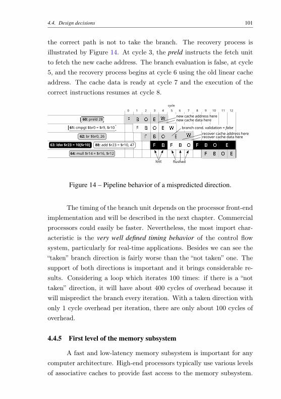
4.4. Design decisions 101
the correct path is not to take the branch. The recovery process isillustrated by Figure 14. At cycle 3, the preld instructs the fetch unitto fetch the new cache address. The branch evaluation is false, at cycle5, and the recovery process begins at cycle 6 using the old linear cacheaddress. The cache data is ready at cycle 7 and the execution of thecorrect instructions resumes at cycle 8.
cycle
61: cmpgt $br0 = $r9, $r10
62: br $br0, 26
64: mull $r14 = $r16, $r12
60: preld 28
0 1 2 3 4 5 6 7 8 9 10
new cache address here
branch cond. validation = false
88: add $r23 = $r10, 4763: ldw $r23 = 10[$r10]
lost
new cache data here
recover cache address hererecover cache data here
flushed
11 12
Figure 14 – Pipeline behavior of a mispredicted direction.
The timing of the branch unit depends on the processor front-endimplementation and will be described in the next chapter. Commercialprocessors could easily be faster. Nevertheless, the most import char-acteristic is the very well defined timing behavior of the control flowsystem, particularly for real-time applications. Besides we can see the“taken” branch direction is fairly worse than the “not taken” one. Thesupport of both directions is important and it brings considerable re-sults. Considering a loop which iterates 100 times: if there is a “nottaken” direction, it will have about 400 cycles of overhead because itwill mispredict the branch every iteration. With a taken direction withonly 1 cycle overhead per iteration, there are only about 100 cycles ofoverhead.
4.4.5 First level of the memory subsystem
A fast and low-latency memory subsystem is important for anycomputer architecture. High-end processors typically use various levelsof associative caches to provide fast access to the memory subsystem.
102 Chapter 4. Thesis rationale and design decisions
However, the use of this approach is not recommended for real-timesystems as discussed in Chapter 2 because it jeopardizes WCET anal-yses.
Recent real-time literature has recommended the use of direct-mapped caches, scratchpad memories or an approach used by Patmosand introduced in Schoeberl (2009a). This approach proposes the useof different caches for different data areas. It is not the purpose of ourwork to propose a new real-time memory architecture. For the firstlevel of the memory subsystem, we use:
∙ instruction memory: direct-mapped cache.
∙ data memory: scratchpad.
Considering the memory subsystem, we contribute with two in-vestigations. First, we investigate how to connect this cache to VLIWpipeline front-end and mainly how the latency of this memory is con-sidered during the WCET analysis. Second, the use of a typical mem-ory access instruction with base plus offset addressing mode introducesadditional latency on the memory instructions, specially for a VLIWprocessor because they have several parallel data paths. We provide aperformance study about using single or multi-port scratchpad accessto diminish the memory latency.
4.4.5.1 Instruction cache
The memory interface connected to the pipeline front-end mustsupply enough data to keep the 4-issue pipeline busy. In VLIW ter-minology, instructions are composed of operations and our four-issuemachine executes up to four operations per cycle forming a 128-bitinstruction word.
Since the main focus of this work is not the memory subsys-tem, any instruction-memory configuration could be used including ascratchpad instruction memory or the method cache presented by PAT-MOS (SCHOEBERL et al., 2011). We used a simple 32-lines of 256-bitblock directed-mapped cache in order to provide sufficient bandwidth
4.4. Design decisions 103
to the pipeline, respect real-time capabilities and to simplify the worst-case execution time analysis. The most important contribution is thecache WCET analysis described in Chapter 6.
4.4.5.2 Data memory interface
The data memory interface was designed to access a scratchpadmemory since we are not considering a complex memory architecturein order to keep a deterministic design.
We considered a unified 32-bit memory address space. Addresses0 to 0x3FFFFFFF (1GiB) are mapped to the instruction memory,0x40000000 to 0x403FFFFF (4MiB) to the scratchpad memory and0x80000000 to 0xFFFFFFFF (2 GiB) to external SDRAM memory.Address space between scratchpad and external SDRAM could be usedfor IO. Data movement between memories (ROM/scratchpad and SD-RAM/ scratchpad) is planned to be done via DMA (Direct MemoryAccess) operations and direct access using memory instructions is onlyavailable for the scratchpad memory. A real-time memory controllerwith a DMA unit is not in the scope of this thesis but it is fully de-scribed in the work of Reineke et al. (2011).
We support base plus offset memory addressing with the follow-ing semantics:
∙ load $rx = immediate_offset [register_base]: loads data from mem-ory with address [ register_base + immediate_offset ] to register$rx.
∙ store immediate_offset [register_base] = $rx: stores the value ofregister $rx to memory with address [ register_base + immedi-ate_offset ].
We target an access to the scratchpad of one cycle, but the en-tire memory instruction transaction is actually a multi-stage operationwith more cycles in order to support base plus offset and byte accessmodes. Memory instructions specification generally determines 2 stagesto perform a memory transaction. One stage is necessary to calculate
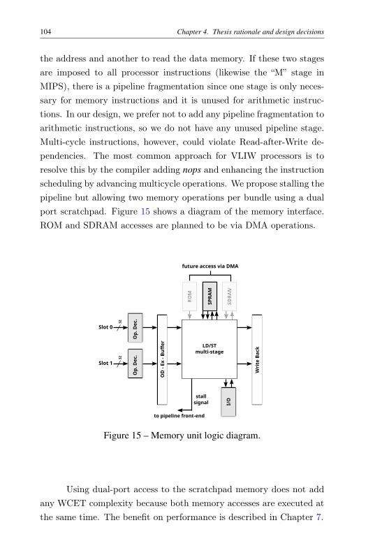
104 Chapter 4. Thesis rationale and design decisions
the address and another to read the data memory. If these two stagesare imposed to all processor instructions (likewise the “M” stage inMIPS), there is a pipeline fragmentation since one stage is only neces-sary for memory instructions and it is unused for arithmetic instruc-tions. In our design, we prefer not to add any pipeline fragmentation toarithmetic instructions, so we do not have any unused pipeline stage.Multi-cycle instructions, however, could violate Read-after-Write de-pendencies. The most common approach for VLIW processors is toresolve this by the compiler adding nops and enhancing the instructionscheduling by advancing multicycle operations. We propose stalling thepipeline but allowing two memory operations per bundle using a dualport scratchpad. Figure 15 shows a diagram of the memory interface.ROM and SDRAM accesses are planned to be via DMA operations.
32
Op.
Dec
.
OD
- Ex
- Bu
ffer
Slot 0
LD/STmulti-stage
32
Op.
Dec
.
Slot 1
Wri
te B
ack
SPRA
M
I/O
ROM
SDRA
M
stallsignal
to pipeline front-end
future access via DMA
Figure 15 – Memory unit logic diagram.
Using dual-port access to the scratchpad memory does not addany WCET complexity because both memory accesses are executed atthe same time. The benefit on performance is described in Chapter 7.
4.4. Design decisions 105
4.4.6 Compiler support
In order to have a compiler for the architecture and to provide acustomizable environment to research real-time compiler capabilities,a new code generator back-end for LLVM (LATTNER; ADVE, 2004)was implemented and it makes part of a different thesis. In this Sectionwe only provide an overview of the back-end.
LLVM is a compiler infrastructure targeted to be modular andextensible. As compiler front-end we used Clang4, which supports C-like languages.
Since the processor has a substantial number of registers, it ispossible to reduce the access to memory data in a compiled program. Asubstantial source of memory operations are the accesses to local vari-ables that are allocated in the procedure stack. Most of the variablesthat are originally allocated in the stack can be promoted to permanentregister variables. This promotion of stack to register variables is doneby a pass called PromoteMemoryToRegisterPass, which already existsin LLVM, and is enabled by the back-end. The execution of this passreduces significantly the number of memory access of programs, due tothe fact that the Clang front-end always allocates local variables in thestack.
Considering instruction ordering to expose ILP to the proces-sor, we used the default VLIW scheduler. This algorithm performstop-down list scheduling locally in each basic block. As input data,the scheduling process uses a simplified description of the processorresources (represented as a hazard recognizer) and a machine code ba-sic block to be scheduled. Instruction scheduling is performed beforethe register allocation process, so the output of this phase is not acomplete machine code representation. There is no global instructionscheduler for VLIW architectures in LLVM. Global instruction sched-ulers can explore ILP across basic block boundaries, resulting in betterperformance when compared with the local ones. Examples of globalschedulers are Superblock Scheduling (HWU et al., 1993) and Trace
4 http://clang.llvm.org/
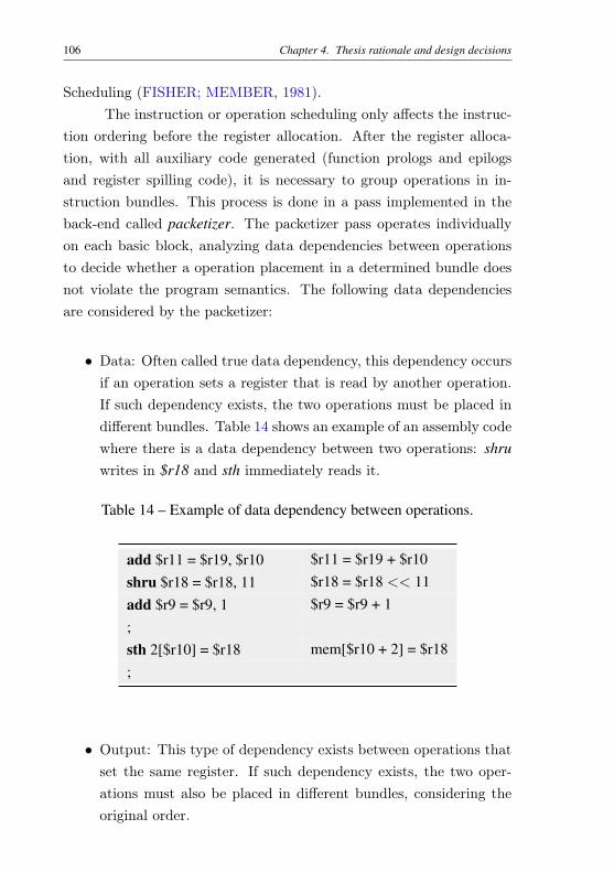
106 Chapter 4. Thesis rationale and design decisions
Scheduling (FISHER; MEMBER, 1981).The instruction or operation scheduling only affects the instruc-
tion ordering before the register allocation. After the register alloca-tion, with all auxiliary code generated (function prologs and epilogsand register spilling code), it is necessary to group operations in in-struction bundles. This process is done in a pass implemented in theback-end called packetizer. The packetizer pass operates individuallyon each basic block, analyzing data dependencies between operationsto decide whether a operation placement in a determined bundle doesnot violate the program semantics. The following data dependenciesare considered by the packetizer:
∙ Data: Often called true data dependency, this dependency occursif an operation sets a register that is read by another operation.If such dependency exists, the two operations must be placed indifferent bundles. Table 14 shows an example of an assembly codewhere there is a data dependency between two operations: shruwrites in $r18 and sth immediately reads it.
Table 14 – Example of data dependency between operations.
add $r11 = $r19, $r10 $r11 = $r19 + $r10shru $r18 = $r18, 11 $r18 = $r18 << 11add $r9 = $r9, 1 $r9 = $r9 + 1;sth 2[$r10] = $r18 mem[$r10 + 2] = $r18;
∙ Output: This type of dependency exists between operations thatset the same register. If such dependency exists, the two oper-ations must also be placed in different bundles, considering theoriginal order.
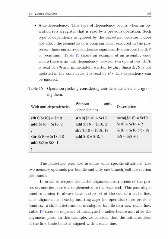
4.4. Design decisions 107
∙ Anti-dependency: This type of dependency occurs when an op-eration sets a register that is read by a previous operation. Suchtype of dependency is ignored by the packetizer because it doesnot affect the semantics of a program when executed in the pro-cessor. Ignoring anti-dependencies significantly improves the ILPof programs. Table 15 shows an example of an assembly codewhere there is an anti-dependency between two operations: $r10is read by sth and immediately written by shr. Since $r10 is notupdated in the same cycle it is read by shr, this dependency canbe ignored.
Table 15 – Operation packing considering anti-dependencies, and ignor-ing them.
With anti-dependenciesWithout anti-dependencies
Description
sth 0[$r10] = $r19 sth 0[$r10] = $r19 mem[$r10] = $r19add $r16 = $r16, 2 add $r16 = $r16, 2 $r16 = $r16 + 2; shr $r10 = $r18, 18 $r10 = $r10 >> 18shr $r10 = $r18, 18 add $r8 = $r8, 1 $r8 = $r8 + 1add $r8 = $r8, 1 ;;
The packetizer pass also assumes some specific situations, liketwo memory operands per bundle and only one branch/call instructionper bundle.
In order to respect the cache alignment restrictions of the pro-cessor, another pass was implemented in the back-end. This pass alignsbundles aiming to always have a stop bit at the end of a cache line.This alignment is done by inserting nops (no operation) into previousbundles, to shift a determined misaligned bundle to a new cache line.Table 16 shows a sequence of misaligned bundles before and after thealignment pass. In this example, we consider that the initial addressof the first basic block is aligned with a cache line.
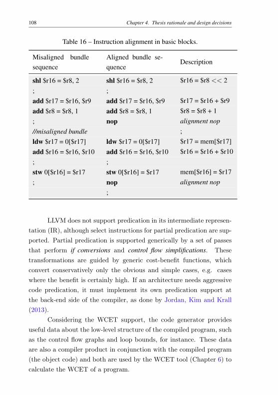
108 Chapter 4. Thesis rationale and design decisions
Table 16 – Instruction alignment in basic blocks.
Misaligned bundlesequence
Aligned bundle se-quence
Description
shl $r16 = $r8, 2 shl $r16 = $r8, 2 $r16 = $r8 << 2; ;add $r17 = $r16, $r9 add $r17 = $r16, $r9 $r17 = $r16 + $r9add $r8 = $r8, 1 add $r8 = $r8, 1 $r8 = $r8 + 1; nop alignment nop
//misaligned bundle ;ldw $r17 = 0[$r17] ldw $r17 = 0[$r17] $r17 = mem[$r17]add $r16 = $r16, $r10 add $r16 = $r16, $r10 $r16 = $r16 + $r10; ;stw 0[$r16] = $r17 stw 0[$r16] = $r17 mem[$r16] = $r17; nop alignment nop
;
LLVM does not support predication in its intermediate represen-tation (IR), although select instructions for partial predication are sup-ported. Partial predication is supported generically by a set of passesthat perform if conversions and control flow simplifications. Thesetransformations are guided by generic cost-benefit functions, whichconvert conservatively only the obvious and simple cases, e.g. caseswhere the benefit is certainly high. If an architecture needs aggressivecode predication, it must implement its own predication support atthe back-end side of the compiler, as done by Jordan, Kim and Krall(2013).
Considering the WCET support, the code generator providesuseful data about the low-level structure of the compiled program, suchas the control flow graphs and loop bounds, for instance. These dataare also a compiler product in conjunction with the compiled program(the object code) and both are used by the WCET tool (Chapter 6) tocalculate the WCET of a program.
4.5. Summary 109
4.5 SUMMARY
We started this Chapter discussing the challenging task of ana-lyzing real-time systems, specially due to the motivation of obtainingsafe and more precise WCET estimations. There are different hardwarerequirements between general-purpose and real-time systems althoughboth of them need constant performance enhancements.
Regarding our objective to improve performance and determin-ism, we exposed several processor architecture features that lead topredictable design but also increases the WCET performance. We havesecured our low-level requirements focusing on hard real-time systemsbut also not forgetting the high-level requirements allowing our designto be applicable to modern systems using a modern ISA and a moderncompiler back-end.
We discussed the design decisions through an architecture over-view. We focus on a real-time processor architecture using a 4-issueVLIW design with 32-bit RISC operations using HP ST231 ISA. Wesupport both types of predication as well as static branch predictionwith well-defined behavior. Table 17 presents a synthesis of real-timeprocessor features considering the standard ST231, PATMOS, PRETand the prototype described in this thesis.
Regarding our contributions for real-time processor architectures,we can highlight:
∙ Low-overhead full-predication system for VLIW processors.
∙ Detailed branch architecture.
∙ VHDL design and timing characteristic.
∙ Complete WCET analysis for the proposed design.
∙ Design space investigation and evaluation.
5 ARMv4 supports full predication, but there is no mention in (LIU et al., 2012) about PREThardware support.
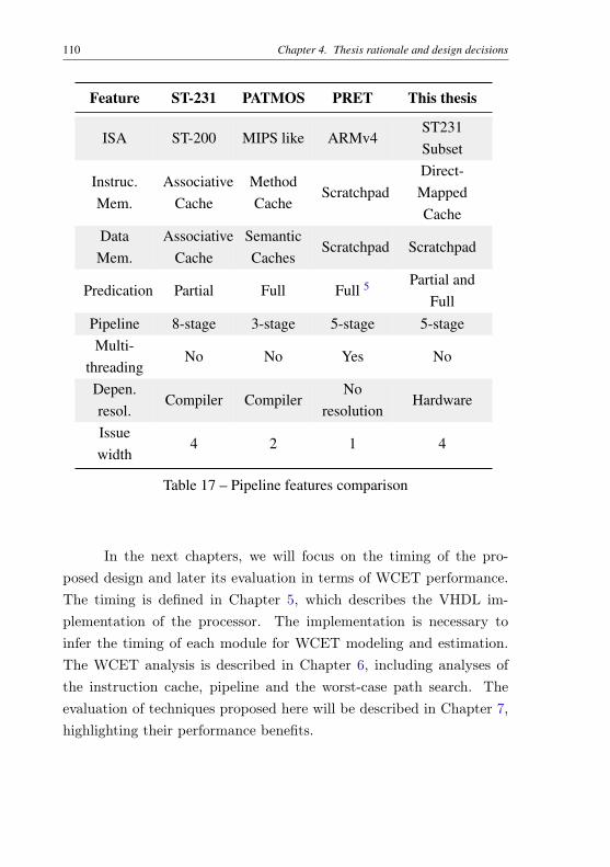
110 Chapter 4. Thesis rationale and design decisions
Feature ST-231 PATMOS PRET This thesis
ISA ST-200 MIPS like ARMv4ST231Subset
Instruc.Mem.
AssociativeCache
MethodCache
ScratchpadDirect-MappedCache
DataMem.
AssociativeCache
SemanticCaches
Scratchpad Scratchpad
Predication Partial Full Full 5 Partial andFull
Pipeline 8-stage 3-stage 5-stage 5-stageMulti-
threadingNo No Yes No
Depen.resol.
Compiler CompilerNo
resolutionHardware
Issuewidth
4 2 1 4
Table 17 – Pipeline features comparison
In the next chapters, we will focus on the timing of the pro-posed design and later its evaluation in terms of WCET performance.The timing is defined in Chapter 5, which describes the VHDL im-plementation of the processor. The implementation is necessary toinfer the timing of each module for WCET modeling and estimation.The WCET analysis is described in Chapter 6, including analyses ofthe instruction cache, pipeline and the worst-case path search. Theevaluation of techniques proposed here will be described in Chapter 7,highlighting their performance benefits.
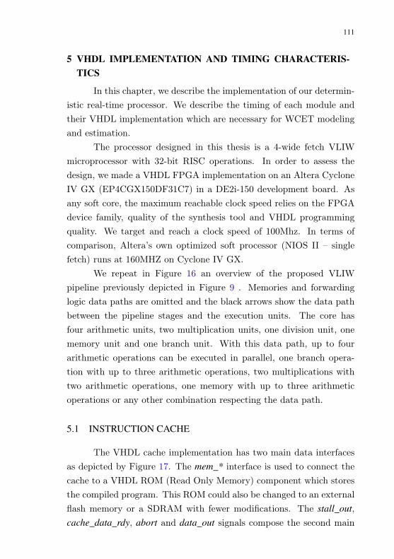
111
5 VHDL IMPLEMENTATION AND TIMING CHARACTERIS-TICS
In this chapter, we describe the implementation of our determin-istic real-time processor. We describe the timing of each module andtheir VHDL implementation which are necessary for WCET modelingand estimation.
The processor designed in this thesis is a 4-wide fetch VLIWmicroprocessor with 32-bit RISC operations. In order to assess thedesign, we made a VHDL FPGA implementation on an Altera CycloneIV GX (EP4CGX150DF31C7) in a DE2i-150 development board. Asany soft core, the maximum reachable clock speed relies on the FPGAdevice family, quality of the synthesis tool and VHDL programmingquality. We target and reach a clock speed of 100Mhz. In terms ofcomparison, Altera’s own optimized soft processor (NIOS II – singlefetch) runs at 160MHZ on Cyclone IV GX.
We repeat in Figure 16 an overview of the proposed VLIWpipeline previously depicted in Figure 9 . Memories and forwardinglogic data paths are omitted and the black arrows show the data pathbetween the pipeline stages and the execution units. The core hasfour arithmetic units, two multiplication units, one division unit, onememory unit and one branch unit. With this data path, up to fourarithmetic operations can be executed in parallel, one branch opera-tion with up to three arithmetic operations, two multiplications withtwo arithmetic operations, one memory with up to three arithmeticoperations or any other combination respecting the data path.
5.1 INSTRUCTION CACHE
The VHDL cache implementation has two main data interfacesas depicted by Figure 17. The mem_* interface is used to connect thecache to a VHDL ROM (Read Only Memory) component which storesthe compiled program. This ROM could also be changed to an externalflash memory or a SDRAM with fewer modifications. The stall_out,cache_data_rdy, abort and data_out signals compose the second main
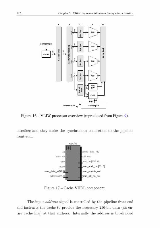
112 Chapter 5. VHDL implementation and timing characteristics
Wri
te B
ack
Ins.
Bun
dle
Dec
odin
g
ALU
ALU
ALU
ALU
Op.
Dec
.
LD/ST
MULDIV
Bran
chU
nit
Slot
0Sl
ot 1
Slot
2Sl
ot 3
256
256
3232
3232
Cach
e Bu
ffer
Op.
Dec
.O
p. D
ec.
Op.
Dec
.
F B O E W
Cache
CacheScratchpad
SDRAM/ROM
SDRAM/ROM
Figure 16 – VLIW processor overview (reproduced from Figure 9).
interface and they make the synchronous connection to the pipelinefront-end.
cache
abort
clk
mem_clk
reset
address[22..0]
mem_data_in[31..0]
cache_data_rdy
mem_enable_out
mem_clk_en_out
stall_out
mem_addr_out[31..0]
data_out[255..0]
Figure 17 – Cache VHDL component.
The input address signal is controlled by the pipeline front-endand instructs the cache to provide the necessary 256-bit data (an en-tire cache line) at that address. Internally the address is bit-divided
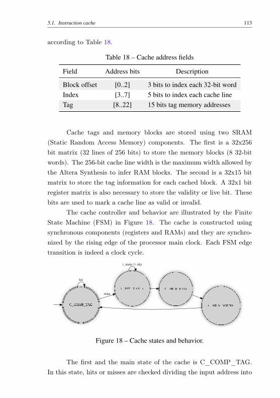
5.1. Instruction cache 113
according to Table 18.
Table 18 – Cache address fields
Field Address bits Description
Block offset [0..2] 3 bits to index each 32-bit wordIndex [3..7] 5 bits to index each cache lineTag [8..22] 15 bits tag memory addresses
Cache tags and memory blocks are stored using two SRAM(Static Random Access Memory) components. The first is a 32x256bit matrix (32 lines of 256 bits) to store the memory blocks (8 32-bitwords). The 256-bit cache line width is the maximum width allowed bythe Altera Synthesis to infer RAM blocks. The second is a 32x15 bitmatrix to store the tag information for each cached block. A 32x1 bitregister matrix is also necessary to store the validity or live bit. Thesebits are used to mark a cache line as valid or invalid.
The cache controller and behavior are illustrated by the FiniteState Machine (FSM) in Figure 18. The cache is constructed usingsynchronous components (registers and RAMs) and they are synchro-nized by the rising edge of the processor main clock. Each FSM edgetransition is indeed a clock cycle.
hit
miss
i_mem != rdy
Figure 18 – Cache states and behavior.
The first and the main state of the cache is C_COMP_TAG.In this state, hits or misses are checked dividing the input address into
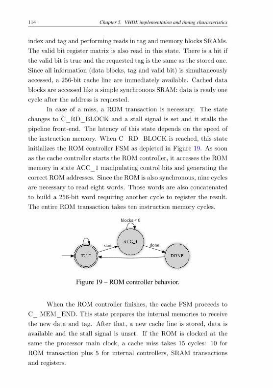
114 Chapter 5. VHDL implementation and timing characteristics
index and tag and performing reads in tag and memory blocks SRAMs.The valid bit register matrix is also read in this state. There is a hit ifthe valid bit is true and the requested tag is the same as the stored one.Since all information (data blocks, tag and valid bit) is simultaneouslyaccessed, a 256-bit cache line are immediately available. Cached datablocks are accessed like a simple synchronous SRAM: data is ready onecycle after the address is requested.
In case of a miss, a ROM transaction is necessary. The statechanges to C_RD_BLOCK and a stall signal is set and it stalls thepipeline front-end. The latency of this state depends on the speed ofthe instruction memory. When C_RD_BLOCK is reached, this stateinitializes the ROM controller FSM as depicted in Figure 19. As soonas the cache controller starts the ROM controller, it accesses the ROMmemory in state ACC_1 manipulating control bits and generating thecorrect ROM addresses. Since the ROM is also synchronous, nine cyclesare necessary to read eight words. Those words are also concatenatedto build a 256-bit word requiring another cycle to register the result.The entire ROM transaction takes ten instruction memory cycles.
start
blocks < 8
done
Figure 19 – ROM controller behavior.
When the ROM controller finishes, the cache FSM proceeds toC_ MEM_END. This state prepares the internal memories to receivethe new data and tag. After that, a new cache line is stored, data isavailable and the stall signal is unset. If the ROM is clocked at thesame the processor main clock, a cache miss takes 15 cycles: 10 forROM transaction plus 5 for internal controllers, SRAM transactionsand registers.
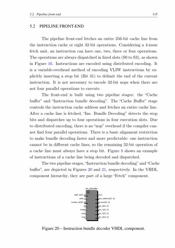
5.2. Pipeline front-end 115
5.2 PIPELINE FRONT-END
The pipeline front-end fetches an entire 256-bit cache line fromthe instruction cache or eight 32-bit operations. Considering a 4-issuefetch unit, an instruction can have one, two, three or four operations.The operations are always dispatched in fixed slots (S0 to S3), as shownin Figure 16. Instructions are encoded using distributed encoding. Itis a variable-overhead method of encoding VLIW instructions by ex-plicitly inserting a stop bit (Bit 31) to delimit the end of the currentinstruction. It is not necessary to encode 32-bit nops when there arenot four parallel operations to execute.
The front-end is built using two pipeline stages: the “Cachebuffer” and “Instruction bundle decoding”. The “Cache Buffer” stagecontrols the instruction cache address and fetches an entire cache line.After a cache line is fetched, “Ins. Bundle Decoding” detects the stopbits and dispatches up to four operations in four execution slots. Dueto distributed encoding, there is no “nop” overhead if the compiler can-not find four parallel operations. There is a basic alignment restrictionto make bundle decoding faster and more predictable: one instructioncannot be in different cache lines, so the remaining 32-bit operation ofa cache line must always have a stop bit. Figure 8 shows an exampleof instructions of a cache line being decoded and dispatched.
The two pipeline stages, “Instruction bundle decoding” and “Cachebuffer”, are depicted in Figures 20 and 21, respectively. In the VHDLcomponent hierarchy, they are part of a large “Fetch” component.
ins_decoder
addr_ld
clk
enable
preld
reset
addr_in[22..0]
bundle_in[255..0]
error
slot_0[31..0]
slot_1[31..0]
slot_2[31..0]
slot_3[31..0]
recover[22..0]
next_address[22..0]
Figure 20 – Instruction bundle decoder VHDL component.
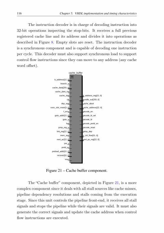
116 Chapter 5. VHDL implementation and timing characteristics
The instruction decoder is in charge of decoding instruction into32-bit operations inspecting the stop-bits. It receives a full previousregistered cache line and its address and divides it into operations asdescribed in Figure 8. Empty slots are reset. The instruction decoderis a synchronous component and is capable of decoding one instructionper cycle. This decoder must also support synchronous load to supportcontrol flow instructions since they can move to any address (any cacheword offset).
cache_buffer
branch_in
cache_data_rdy
cache_stall
clk
dep_stall
f_error
goto_in
halt
jump_reg_in
mem_stall
pre_jr
preld_en
reset
next_pc[22..0]
cache_data[255..0]
link_reg[22..0]
b_address[22..0]
goto_addr[22..0]
preload_addr[22..0]
exec_slot_mask[3..0]
recover[22..0]
cache_abort
decode_en
decode_ld
decode_ld_sel
decode_preld_en
decode_reset
delay_dep
next_pc_reg[22..0]
bundle_out[255..0]
b_address_reg[22..0]
n_ctrl_flow[31..0]
cache_address[22..0]
Figure 21 – Cache buffer component.
The “Cache buffer” component, depicted in Figure 21, is a morecomplex component since it deals with all stall sources like cache misses,pipeline dependency resolutions and stalls coming from the executionstage. Since this unit controls the pipeline front-end, it receives all stallsignals and stops the pipeline while their signals are valid. It must alsogenerate the correct signals and update the cache address when controlflow instructions are executed.
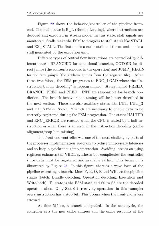
5.2. Pipeline front-end 117
Figure 22 shows the behavior/controller of the pipeline front-end. The main state is B_L (Bundle Loading), where instructions aredecoded and executed in stream mode. In this state, stall signals aremonitored. Stalls make the FSM to progress to stall states like STALLand EX_STALL. The first one is a cache stall and the second one is astall generated by the execution unit.
Different types of control flow instructions are controlled by dif-ferent states: BRANCHIN for conditional branches, GOTOIN for di-rect jumps (the address is encoded in the operation) and JUMP_REGINfor indirect jumps (the address comes from the register file). Afterthese transitions, the FSM progresses to ENC_LOAD where the “In-struction bundle decoding” is reprogrammed. States named PRELD,BRANCH_PRED and PRED_ INIT are responsible for branch pre-diction. The branch behavior and timing will be better described inthe next section. There are also auxiliary states like INIT, INIT_2and EX_STALL_SYNC_2 which are necessary to enable data to becorrectly registered during the FSM progression. The states HALTEDand ENC_ERROR are reached when the CPU is halted by a halt in-struction or when there is an error in the instruction decoding (cachealignment/stop bits missing).
The front-end controller was one of the most challenging parts ofthe processor implementation, specially to reduce unnecessary latenciesand to keep a synchronous implementation. Avoiding latches on usingregisters enhances the VHDL synthesis but complicates the controllersince data must be registered and available earlier. This behavior isillustrated by Figure 23. In this figure, there is a wave form of thepipeline executing a branch. Lines F, B, O, E and WB are the pipelinestages (Fetch, Bundle decoding, Operation decoding, Execution andWrite-back). F_state is the FSM state and S0 to S3 are the decodedoperation slots. Only Slot 0 is receiving operations in this example:every instruction has a stop bit. This occurs when the front-end is lessstressed.
At time 515 ns, a branch is signaled. In the next cycle, thecontroller sets the new cache address and the cache responds at the
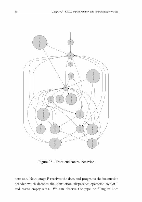
118 Chapter 5. VHDL implementation and timing characteristics
IDLE
STALL
HALTED
ENC_ERROR
INIT
GOTOIN
JUMP_REGIN
BRANCHIN
B_L
EXSTALL
PRELD
INIT_2
FLOW_STALL
EX_STALL_SYNC
ENC_LOAD
FLOW_EXSTALL
BRANCH_PRED
PRED_IN
IT
Figure 22 – Front-end control behavior.
next one. Next, stage F receives the data and programs the instructiondecoder which decodes the instruction, dispatches operation to slot 0and resets empty slots. We can observe the pipeline filling in lines
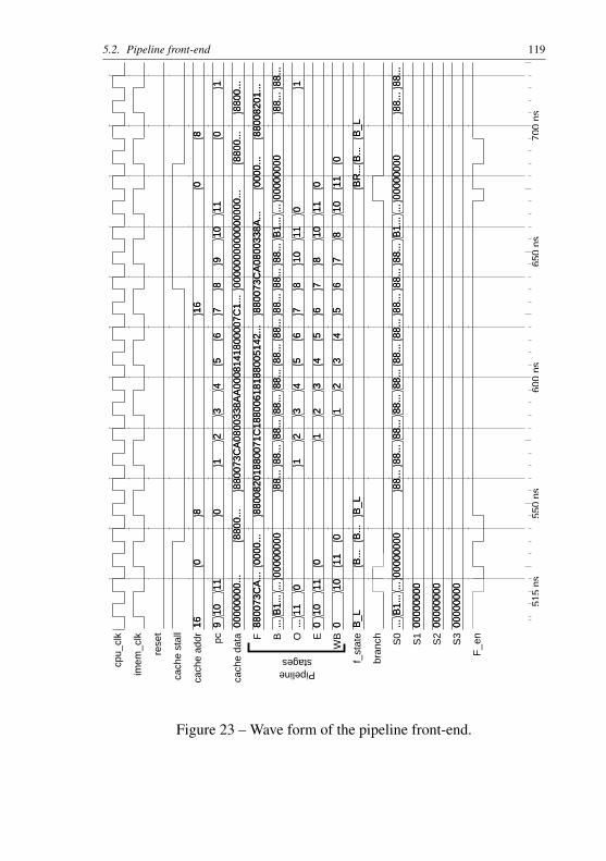
5.2. Pipeline front-end 119
160
816
08
910
110
12
34
56
78
910
110
1
0000
0000
...88
00...
8800
73C
A08
0033
8AA
0008
1418
0000
7C1.
..00
0000
0000
0000
00...
8800
...88
00...
8800
73C
A...
0000
...88
0082
0188
0071
C18
8006
1818
8005
142.
..88
0073
CA
0800
338A
...00
00...
8800
8201
...
...B
1...
...00
0000
0088
...88
...88
...88
...88
...88
...88
...88
...88
...88
...B
1...
...00
0000
0088
...88
...
...11
01
23
45
67
810
110
1
010
110
12
34
56
78
1011
0
010
110
12
34
56
78
1011
0
B_L
B...
B...
B_L
BR
...B
...B
_L
...B
1...
...00
0000
0088
...88
...88
...88
...88
...88
...88
...88
...88
...88
...B
1...
...00
0000
0088
...88
...
0000
0000
0000
0000
0000
0000
550
ns60
0 ns
650
ns70
0 ns
cpu_
clk
imem
_clk
rese
t
cach
e st
all
cach
e ad
dr16
08
160
8
pc9
1011
01
23
45
67
89
1011
01
cach
e da
ta00
0000
00...
8800
...88
0073
CA
0800
338A
A00
0814
1800
007C
1...
0000
0000
0000
0000
...88
00...
8800
...
F88
0073
CA
...00
00...
8800
8201
8800
71C
1880
0618
1880
0514
2...
8800
73C
A08
0033
8A...
0000
...88
0082
01...
B...
B1.
.....
0000
0000
88...
88...
88...
88...
88...
88...
88...
88...
88...
88...
B1.
.....
0000
0000
88...
88...
O...
110
12
34
56
78
1011
01
E0
1011
01
23
45
67
810
110
WB
010
110
12
34
56
78
1011
0
f_st
ate
B_L
B...
B...
B_L
BR
...B
...B
_L
bran
ch S0
...B
1...
...00
0000
0088
...88
...88
...88
...88
...88
...88
...88
...88
...88
...B
1...
...00
0000
0088
...88
...
S1
0000
0000
S2
0000
0000
S3
0000
0000
F_e
n
Pipelinestages
515
ns
Figure 23 – Wave form of the pipeline front-end.
120 Chapter 5. VHDL implementation and timing characteristics
F to WB. Considering timing, we can note that to produce a decodedoperation in slot 0 at 545ns, the cache was programmed at 515ns. Whenthe fetch operates in full stream mode with 4 operations per cycle,a cache line address is generated on every cycle and this behavior isdynamic since instructions may have 1, 2, 3 or 4 operations. Thefront-end must control the pipeline considering possible high timingstall cycles, possible dependencies with one stall cycle, control flowinstructions and dynamic instruction size.
5.3 THE CONTROL-FLOW SYSTEM
The control-flow system is composed by the branch unit and bythe pipeline front-end. The front-end, as indicated earlier, controlsthe cache considering its signals, timing and address. It also controlsinstruction decoding. The branch unit, on the other side, instructsthe front end when there are control-flow operations, evaluates theconditions for conditional branches and calculates the correct targetaddresses.
The processor branch unit takes care of all control flow oper-ations including direct, indirect and conditional jumps. They mustalways be encoded in the first operation of an instruction: the branchunit is connected only to Slot S0 data path as shown in Figure 16.Conditional branch instructions are encoded with a binary predicate($br) and a 23-bit offset parameter relative to the program counter(23-bit immediate). Branch conditions are calculated separately fromthe branch operation using arithmetic operations. Direct jumps alsouse a 23-bit offset parameter relative to the program counter. Indirectjumps use the address specified in the register without offset.
In order to perform a control-flow operation, the processor mustdecode the correct control-flow type, perform the address calculationand reprogram the pipeline front end. The control-flow system is incharge of detecting the control-flow type and calculating the targetaddress. It signals the front end to reprogram the fetch unit providingthe correct target address and the control-flow type. Cache transactions
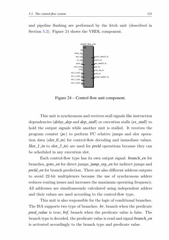
5.3. The control-flow system 121
and pipeline flushing are performed by the fetch unit (described inSection 5.2). Figure 24 shows the VHDL component.
control_flow_unit
clk
delay_dep
dep_stall
ex_stall
pred_value
reset
slot_0_in[31..0]
slot_1_in[31..0]
slot_2_in[31..0]
slot_3_in[31..0]
pc[22..0]
branch_en
goto_en
jump_reg_en
preld_en
branch_addr[22..0]
goto_addr[22..0]
preload_addr[22..0]
Figure 24 – Control flow unit component.
This unit is synchronous and receives stall signals like instructiondependencies (delay_dep and dep_stall) or execution stalls (ex_stall) tohold the output signals while another unit is stalled. It receives theprogram counter (pc) to perform PC relative jumps and slot opera-tion data (slot_0_in) for control-flow decoding and immediate values.Slot_1_in to slot_3_in) are used for preld operations because they canbe scheduled in any execution slot.
Each control-flow type has its own output signal: branch_en forbranches, goto_en for direct jumps, jump_reg_en for indirect jumps andpreld_en for branch prediction. There are also different address outputsto avoid 22-bit multiplexers because the use of synchronous addersreduces routing issues and increases the maximum operating frequency.All addresses are simultaneously calculated using independent addersand their values are used according to the control-flow type.
This unit is also responsible for the logic of conditional branches.The ISA supports two type of branches: br, branch when the predicatepred_value is true; brf, branch when the predicate value is false. Thebranch type is decoded, the predicate value is read and signal branch_enis activated accordingly to the branch type and predicate value.
122 Chapter 5. VHDL implementation and timing characteristics
5.4 REGISTER FILES
The register file is the primary and the fastest data storage area.In the case of a RISC processor, all processing data must be in theregister file to be manipulated. Essentially, the register file is an arrayof registers and it must provide fast and dynamic access.
A register file of a single-fetch processor must provide at leasttwo read and one write ports. Two read ports are necessary to readinstruction operands while a write port is utilized to write processingresults. In the case of pipelined processors, those ports are accessed inevery clock cycle since operands are read in earlier pipeline stages andthe result of further instruction is stored in the write-back phase.
For VLIW processors, the register file is even more complex. A4-issue machine needs to read eight operands (two for each slot) andwrite four results at every cycle. This gives a total of twelve dynamicaccess ports. Those ports should also provide simultaneous access toevery register address and forward a fresh result to a reading port if awrite occurs at the same cycle. Multi-ported register files are typicallyconstructed with expensive specialized SRAMs (Static RAMs) sinceconventional SRAMs provide only two ports.
In the context of this thesis, two register files are necessary withthe following characteristics:
∙ General purpose register file:
– 8 read ports.
– 4 write ports.
– 64 general purpose 32-bit registers (6 address bits).
– Internal forward unit (writes are immediately forwarded toread ports).
∙ Predicates register file:
– 4 read ports.
– 1 fixed read port for full predication ($br4).
5.4. Register files 123
– 8 1-bit predicate/branch registers (3 address bits).
– Internal forward unit (writes are immediately forwarded toread ports).
There are many ways to implement a register file in FPGA. Usingonly combinational logic (register/latches) does not produce an efficientdesign. As FPGAs have lots of memory blocks, it is better to usethem to store register file data. Unfortunately FPGA RAM blocksusually have just 2 ports: 1 for reading and 1 for writing. Therefore,to efficiently implement a register file, we need to replicate the memoryblocks and track the most recent copy. For instance, if we have 4 writeports, we have 4 copies of the registers. The problem is how to trackthe most recent value in a read operation.
There are two recent works, (LAFOREST; STEFFAN, 2010) and(LAFOREST et al., 2012), that show how to efficiently track the mostrecent copy. The first one uses a structure called Live Value Table(LVT) that stores the write port number in a write operation and thisvalue is used to multiplex the recent value in a read operation (all copiesof the register file are read at the same time). LVT is implemented usingonly logic elements because it needs the same number of write and readports as the register file but it needs much fewer hardware resourcesthan a whole register file implemented with logic elements.
In the second work (LAFOREST et al., 2012), they use XORoperations to track the most recent copy. Bitwise XOR is commutative,associative and it has 3 interesting properties: A⊕0 = A, B⊕B = 0 andA⊕B⊕B = A. In this implementation, a value that has to be writtenin a bank is first XORED with all other replicated banks. On a read,the register file returns the most recent value using the same XORoperation doing XOR of all replicated banks and returning the mostrecent one. The drawback of the XOR design is that each write requiresreading, since we must store the write value XOR the old value of thatlocation from the other bank. This increases the number of FPGAmemories required to implement the design and the register file mustbe clocked twice as fast as the pipeline. The LVT design uses more logic
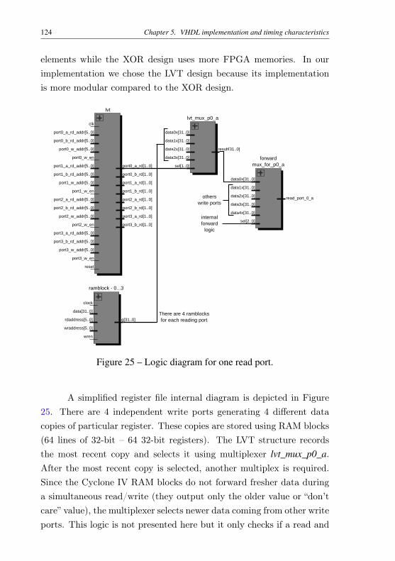
124 Chapter 5. VHDL implementation and timing characteristics
elements while the XOR design uses more FPGA memories. In ourimplementation we chose the LVT design because its implementationis more modular compared to the XOR design.
lvt
clk
port0_w_en
port1_w_en
port2_w_en
port3_w_en
reset
port0_w_addr[5..0]
port1_w_addr[5..0]
port2_w_addr[5..0]
port3_w_addr[5..0]
port0_a_rd_addr[5..0]
port0_b_rd_addr[5..0]
port1_a_rd_addr[5..0]
port1_b_rd_addr[5..0]
port2_a_rd_addr[5..0]
port2_b_rd_addr[5..0]
port3_a_rd_addr[5..0]
port3_b_rd_addr[5..0]
port0_a_rd[1..0]
port0_b_rd[1..0]
port1_a_rd[1..0]
port1_b_rd[1..0]
port2_a_rd[1..0]
port2_b_rd[1..0]
port3_a_rd[1..0]
port3_b_rd[1..0]
forwardmux_for_p0_a
data0x[31..0]
data1x[31..0]
data2x[31..0]
data3x[31..0]
data4x[31..0]
sel[2..0]
read_port_0_a
internalforward
logic
otherswrite ports
ramblock - 0...3
clock
wren
data[31..0]
rdaddress[5..0]
wraddress[5..0]
q[31..0]
lvt_mux_p0_a
data0x[31..0]
data1x[31..0]
data2x[31..0]
data3x[31..0]
sel[1..0]
result[31..0]
There are 4 ramblocksfor each reading port
Figure 25 – Logic diagram for one read port.
A simplified register file internal diagram is depicted in Figure25. There are 4 independent write ports generating 4 different datacopies of particular register. These copies are stored using RAM blocks(64 lines of 32-bit – 64 32-bit registers). The LVT structure recordsthe most recent copy and selects it using multiplexer lvt_mux_p0_a.After the most recent copy is selected, another multiplex is required.Since the Cyclone IV RAM blocks do not forward fresher data duringa simultaneous read/write (they output only the older value or “don’tcare” value), the multiplexer selects newer data coming from other writeports. This logic is not presented here but it only checks if a read and
5.5. Predication support 125
write occur simultaneously and selects the correct/newer data. TheLVT manages a total of 32 RAM blocks: 8 read ports with 4 writeports require 32 copies of the registers.
In order to improve the register file implementation since LVTuses too much memory and bitwise XORs requires a pipelined registerfile, we can use temporary register attached to each functional unit.This technique was used in (SANTOS; AZEVEDO; ARAUJO, 2006)and present interesting results. Temporary registers in each functionalunit minimize the pressure over the global register file and could alsoreduce the overall number of register file ports. On choosing this tech-nique, we also must optimize the register allocation in the compiler.
5.5 PREDICATION SUPPORT
Typically, supporting full predication adds considerable levels oflogic to critical processor data paths (FISHER; FARABOSHI; YOUNG,2005), specially in instruction encoding and forwarding paths. How-ever, the proposed method uses an available encoding bit and does notadd logic to the forwarding paths since only dual paths with only onepredicate is considered. Besides being simple, it does not diminish thepredication capabilities.
Like other registers, predicate register $br4 is read immediatelyafter a VLIW instruction is decoded into S0 to S3 operation slots duringthe “Operation Decoding – O” pipeline stage. Since $br4 must be readin every cycle, an additional fixed address read port is added to thepredicate register file. Adding this new port to this register file has alow impact since there are only 8 1-bit registers and its read addressis fixed. Compared to the general purpose register file which has 1232-bit ports, the predicate register file is considerably simpler having 91-bit ports (5 read ports and 4 write ports).
After the operations are decoded and before they are executedby the arithmetic and memory units, they are registered in a inter-stage pipeline buffer as illustrated in Figure 26. The deactivation logicis executed by the “OD - EX - Buffer”. This buffer is a synchronous
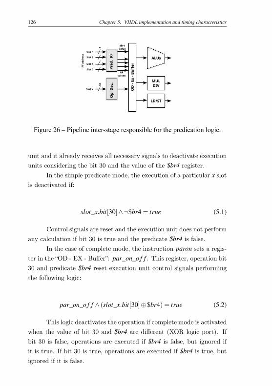
126 Chapter 5. VHDL implementation and timing characteristics
ALUs
32
Op.
Dec
.Pr
ed.
RF
OD
- Ex
- Bu
ffer
Slot x
Slot 0
3
Slot 1
Slot 2
Slot 3
RF a
ddre
ss
LD/ST
MULDIV
RF values
$br4 value
Figure 26 – Pipeline inter-stage responsible for the predication logic.
unit and it already receives all necessary signals to deactivate executionunits considering the bit 30 and the value of the $br4 register.
In the simple predicate mode, the execution of a particular x slotis deactivated if:
slot_x.bit[30]∧¬$br4 = true (5.1)
Control signals are reset and the execution unit does not performany calculation if bit 30 is true and the predicate $br4 is false.
In the case of complete mode, the instruction paron sets a regis-ter in the “OD - EX - Buffer”: par_on_o f f . This register, operation bit30 and predicate $br4 reset execution unit control signals performingthe following logic:
par_on_o f f ∧ (slot_x.bit[30]⊕$br4) = true (5.2)
This logic deactivates the operation if complete mode is activatedwhen the value of bit 30 and $br4 are different (XOR logic port). Ifbit 30 is false, operations are executed if $br4 is false, but ignored ifit is true. If bit 30 is true, operations are executed if $br4 is true, butignored if it is false.
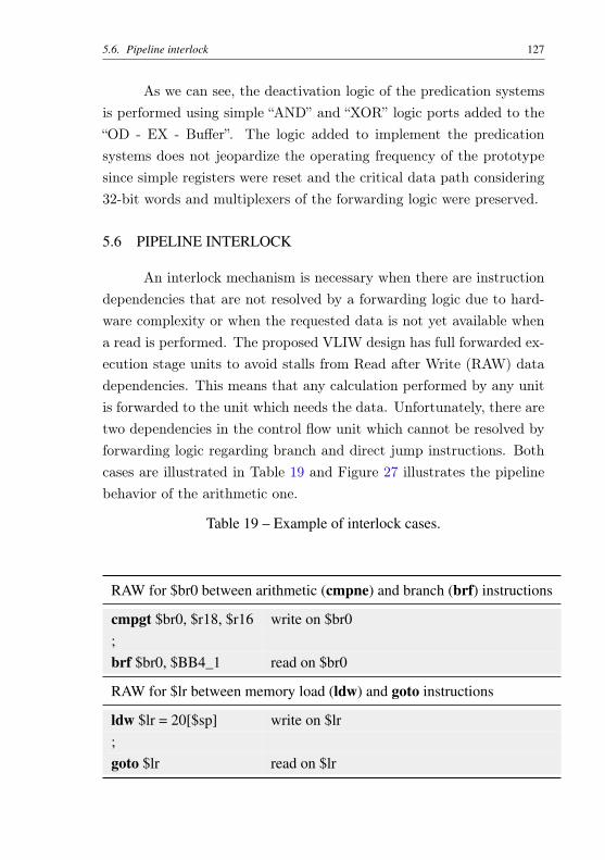
5.6. Pipeline interlock 127
As we can see, the deactivation logic of the predication systemsis performed using simple “AND” and “XOR” logic ports added to the“OD - EX - Buffer”. The logic added to implement the predicationsystems does not jeopardize the operating frequency of the prototypesince simple registers were reset and the critical data path considering32-bit words and multiplexers of the forwarding logic were preserved.
5.6 PIPELINE INTERLOCK
An interlock mechanism is necessary when there are instructiondependencies that are not resolved by a forwarding logic due to hard-ware complexity or when the requested data is not yet available whena read is performed. The proposed VLIW design has full forwarded ex-ecution stage units to avoid stalls from Read after Write (RAW) datadependencies. This means that any calculation performed by any unitis forwarded to the unit which needs the data. Unfortunately, there aretwo dependencies in the control flow unit which cannot be resolved byforwarding logic regarding branch and direct jump instructions. Bothcases are illustrated in Table 19 and Figure 27 illustrates the pipelinebehavior of the arithmetic one.
Table 19 – Example of interlock cases.
RAW for $br0 between arithmetic (cmpne) and branch (brf) instructions
cmpgt $br0, $r18, $r16 write on $br0;brf $br0, $BB4_1 read on $br0
RAW for $lr between memory load (ldw) and goto instructions
ldw $lr = 20[$sp] write on $lr;goto $lr read on $lr

128 Chapter 5. VHDL implementation and timing characteristics
cycle
61: cmpgt $br0 = $r18, $r16
62: br $br0, $BB4_1
0 1 2 3 4 5 6
cmpgt is still executingwhile br needs the value of $br0
61: cmpgt $br0 = $r18, $r16
62: br $br0, $BB4_1
one cycle stall
Figure 27 – Pipeline behavior of interlock RAW dependency.
The interlock is a hardware protection and it is only activatedwhen those instructions are executed subsequently. In both cases, thereis a stall cycle which can be avoided when the compiler schedules a nondependent instruction before the control-flow one.
The interlock is implemented comparing control signals between“Execution” (E) and the “Operation Decoding” (O) stages. The com-plete logic is described in Algorithm 1.
The RAW branch interlock compares the predicate register (br−branch_reg), read for the branch operation during the “O” stage, withthe predicate register destination written during the “E” stage. Whenthere is subsequent read and write, the signal branch_wb_en will betrue as well as the destination and read branch register addresses willbe equal. In this case, the signal ctrl_ f low_stall instructs the pipelinefront end to stop. Since the “E” stage continues to execute, as soon asthe arithmetic instruction follows to the next pipeline stage, interlocklogic will be false and the front-end resumes the pipeline execution.We only consider a reading register in the slot_0 because control-flowoperations are only scheduled in the slot_0 data path.
The RAW goto interlock works like the branch one. First, itchecks whether there is a goto operation in slot_0 and then it checks ifthe goto operation reads the same register address of the memory loadoperation (mem_reg_dest). The goto interlock has only two statementsbecause memory operations are only scheduled in slot_0 and slot_1.
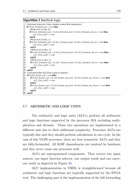
5.7. Arithmetic and Logic units 129
Algorithm 1 Interlock logic1: {Activated when slot_0 has a branch control flow instruction}2: if O.slot_0.branch_op = true then3: {Write in br in Slot_0}4: if O.slot_0.branch_reg = E.slot_0.branch_dest ∧E.slot_0.branch_wb_en = true then5: ctrl_ f low_stall := true6: end if7: {Write in br in Slot_1}8: if O.slot_0.branch_reg = E.slot_1.branch_dest ∧E.slot_1.branch_wb_en = true then9: ctrl_ f low_stall := true
10: end if11: {Write in br in Slot_2}12: if O.slot_0.branch_reg = E.slot_2.branch_dest ∧E.slot_2.branch_wb_en = true then13: ctrl_ f low_stall := true14: end if15: {Write in br in Slot_3}16: if O.slot_0.branch_reg = E.slot_3.branch_dest ∧E.slot_3.branch_wb_en = true then17: ctrl_ f low_stall := true18: end if19: end if20: {Activated when slot_0 has a goto to register}21: if O.slot_0.goto_op = true then22: if O.slot_0.goto_reg = E.slot_0.mem_reg_dest ∧E.slot_0.mem_reg_wb_en = true then23: ctrl_ f low_stall := true24: end if25: if O.slot_0.goto_reg = E.slot_0.mem_reg_dest ∧E.slot_0.mem_reg_wb_en = true then26: ctrl_ f low_stall := true27: end if28: end if
5.7 ARITHMETIC AND LOGIC UNITS
The arithmetic and logic units (ALUs) perform all arithmeticand logic functions supported by the processor ISA excluding multi-plication and division. Those two operations are implemented in adifferent unit due to their additional complexity. Processor ALUs aretypically fast and they should perform calculations in one cycle. In thecase of this VLIW processor, there are four symmetric ALUs and theyare fully-forwarded. All RAW dependencies are resolved by hardwareand they never cause any processor stall.
ALUs are reprogrammed components. They receive two inputsources, one input function selector, one output result and one carry-out result as depicted by Figure 28.
ALU implementation in VHDL is straightforward because allarithmetic and logic functions are typically supported by the FPGAtool. The challenging part is the implementation of the full forwarding
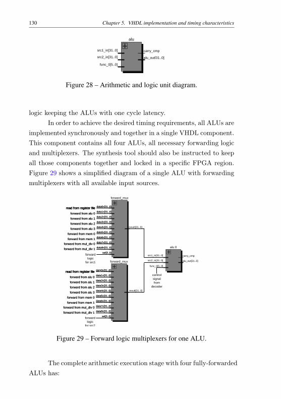
130 Chapter 5. VHDL implementation and timing characteristics
alu
src1_in[31..0]
func_0[5..0]
carry_cmp
alu_out[31..0]src2_in[31..0]
Figure 28 – Arithmetic and logic unit diagram.
logic keeping the ALUs with one cycle latency.In order to achieve the desired timing requirements, all ALUs are
implemented synchronously and together in a single VHDL component.This component contains all four ALUs, all necessary forwarding logicand multiplexers. The synthesis tool should also be instructed to keepall those components together and locked in a specific FPGA region.Figure 29 shows a simplified diagram of a single ALU with forwardingmultiplexers with all available input sources.
alu 0
controlsignalfrom
decoder
src1_in[31..0]
func_0[5..0]
carry_cmp
alu_out[31..0]src2_in[31..0]
forward_mux
data0x[31..0]
data1x[31..0]
data2x[31..0]
data3x[31..0]
data4x[31..0]
data5x[31..0]
data6x[31..0]
data7x[31..0]
data8x[31..0]
sel[3..0]
result[31..0]
result[31..0]
forwardlogic
for src1
read from register fileread from register file
forward from alu 0
forward from alu 1
forward from alu 2
forward from alu 3
forward from mem 0
forward from mem 1
forward from mul_div 0
forward from mul_div 1
data0x[31..0]
data1x[31..0]
data2x[31..0]
data3x[31..0]
data4x[31..0]
data5x[31..0]
data6x[31..0]
data7x[31..0]
data8x[31..0]
sel[3..0]
read from register fileread from register file
forward from alu 0
forward from alu 1
forward from alu 2
forward from alu 3
forward from mem 0
forward from mem 1
forward from mul_div 0
forward from mul_div 1
forward_mux
data0x[31..0]
data1x[31..0]
data2x[31..0]
data3x[31..0]
data4x[31..0]
data5x[31..0]
data6x[31..0]
data7x[31..0]
data8x[31..0]
sel[3..0]forward
logicfor src2
read from register fileread from register file
forward from alu 0
forward from alu 1
forward from alu 2
forward from alu 3
forward from mem 0
forward from mem 1
forward from mul_div 0
forward from mul_div 1
data0x[31..0]
data1x[31..0]
data2x[31..0]
data3x[31..0]
data4x[31..0]
data5x[31..0]
data6x[31..0]
data7x[31..0]
data8x[31..0]
sel[3..0]
read from register fileread from register file
forward from alu 0
forward from alu 1
forward from alu 2
forward from alu 3
forward from mem 0
forward from mem 1
forward from mul_div 0
forward from mul_div 1
Figure 29 – Forward logic multiplexers for one ALU.
The complete arithmetic execution stage with four fully-forwardedALUs has:
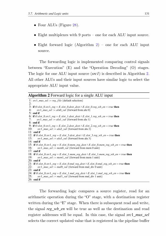
5.7. Arithmetic and Logic units 131
∙ Four ALUs (Figure 28).
∙ Eight multiplexes with 9 ports – one for each ALU input source.
∙ Eight forward logic (Algorithm 2) – one for each ALU inputsource.
The forwarding logic is implemented comparing control signalsbetween “Execution” (E) and the “Operation Decoding” (O) stages.The logic for one ALU input source (src1) is described in Algorithm 2.All other ALUs and their input sources have similar logic to select theappropriate ALU input value.
Algorithm 2 Forward logic for a single ALU input1: src1_mux_sel := reg_ f ile {default selection}2:3: if O.slot_0.src1_reg = E.slot_0.dest_dest ∧E.slot_0.reg_wb_en = true then4: src1_mux_sel := alu0_val {forward from alu 0}5: end if6: if O.slot_0.src1_reg = E.slot_1.dest_dest ∧E.slot_1.reg_wb_en = true then7: src1_mux_sel := alu1_val {forward from alu 1}8: end if9: if O.slot_0.src1_reg = E.slot_2.dest_dest ∧E.slot_2.reg_wb_en = true then
10: src1_mux_sel := alu2_val {forward from alu 2}11: end if12: if O.slot_0.src1_reg = E.slot_3.dest_dest ∧E.slot_3.reg_wb_en = true then13: src1_mux_sel := alu3_val {forward from alu 3}14: end if15: if O.slot_0.src1_reg = E.slot_0.mem_reg_dest ∧E.slot_0.mem_reg_wb_en = true then16: src1_mux_sel := mem0_val {forward from mem 0 unit}17: end if18: if O.slot_0.src1_reg = E.slot_1.mem_reg_dest ∧E.slot_1.mem_reg_wb_en = true then19: src1_mux_sel := mem1_val {forward from mem 1 unit}20: end if21: if O.slot_0.src1_reg = E.slot_0.mul_reg_dest ∧E.slot_0.mul_reg_wb_en = true then22: src1_mux_sel := mul0_val {forward from mul_div 0 unit}23: end if24: if O.slot_0.src1_reg = E.slot_1.mul_reg_dest ∧E.slot_1.mul_reg_wb_en = true then25: src1_mux_sel := mul1_val {forward from mul_div 1 unit}26: end if
The forwarding logic compares a source register, read for anarithmetic operation during the “O” stage, with a destination registerwritten during the “E” stage. When there is subsequent read and write,the signal reg_wb_en will be true as well as the destination and readregister addresses will be equal. In this case, the signal src1_mux_selselects the correct updated value that is registered in the pipeline buffer
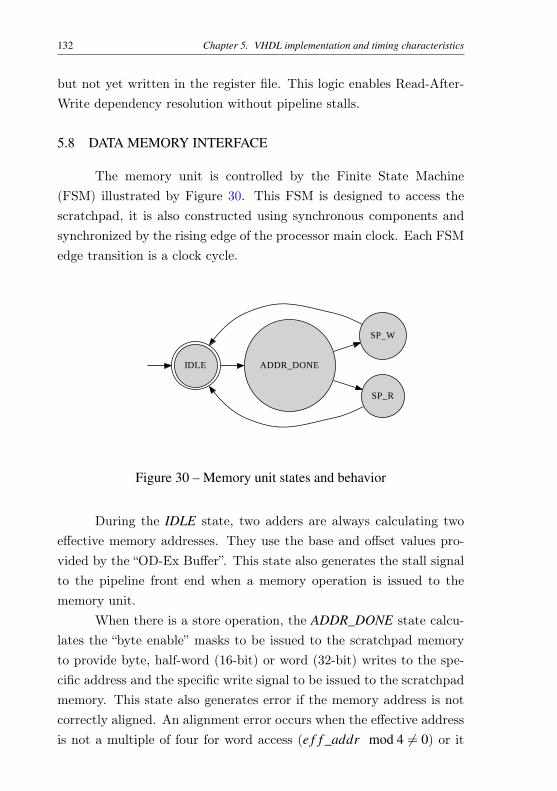
132 Chapter 5. VHDL implementation and timing characteristics
but not yet written in the register file. This logic enables Read-After-Write dependency resolution without pipeline stalls.
5.8 DATA MEMORY INTERFACE
The memory unit is controlled by the Finite State Machine(FSM) illustrated by Figure 30. This FSM is designed to access thescratchpad, it is also constructed using synchronous components andsynchronized by the rising edge of the processor main clock. Each FSMedge transition is a clock cycle.
IDLE ADDR_DONE
SP_W
SP_R
Figure 30 – Memory unit states and behavior
During the IDLE state, two adders are always calculating twoeffective memory addresses. They use the base and offset values pro-vided by the “OD-Ex Buffer”. This state also generates the stall signalto the pipeline front end when a memory operation is issued to thememory unit.
When there is a store operation, the ADDR_DONE state calcu-lates the “byte enable” masks to be issued to the scratchpad memoryto provide byte, half-word (16-bit) or word (32-bit) writes to the spe-cific address and the specific write signal to be issued to the scratchpadmemory. This state also generates error if the memory address is notcorrectly aligned. An alignment error occurs when the effective addressis not a multiple of four for word access (e f f _addr mod 4 ̸= 0) or it
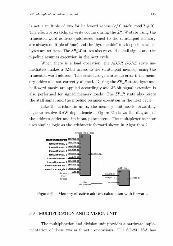
5.9. Multiplication and division unit 133
is not a multiple of two for half-word access (e f f _addr mod 2 ̸= 0).The effective scratchpad write occurs during the SP_W state using thetruncated word address (addresses issued to the scratchpad memoryare always multiple of four) and the “byte enable” mask specifies whichbytes are written. The SP_W states also resets the stall signal and thepipeline resumes execution in the next cycle.
When there is a load operation, the ADDR_DONE state im-mediately makes a 32-bit access to the scratchpad memory using thetruncated word address. This state also generates an error if the mem-ory address is not correctly aligned. During the SP_R state, byte andhalf-word masks are applied accordingly and 32-bit signal extension isalso performed for signed memory loads. The SP_R state also resetsthe stall signal and the pipeline resumes execution in the next cycle.
Like the arithmetic units, the memory unit needs forwardinglogic to resolve RAW dependencies. Figure 31 shows the diagram ofthe address adder and its input parameters. The multiplexer selectoruses similar logic as the arithmetic forward shown in Algorithm 2.
addr_addr
dataa[31..0]
clk
result[31..0]datab[31..0]
forward_mux - base
data0x[31..0]
data1x[31..0]
data2x[31..0]
data3x[31..0]
data4x[31..0]
data5x[31..0]
data6x[31..0]
data7x[31..0]
data8x[31..0]
sel[3..0]
result[31..0]
forwardlogic
for src1
read from register fileread from register file
forward from alu 0
forward from alu 1
forward from alu 2
forward from alu 3
forward from mem 0
forward from mem 1
forward from mul_div 0
forward from mul_div 1
data0x[31..0]
data1x[31..0]
data2x[31..0]
data3x[31..0]
data4x[31..0]
data5x[31..0]
data6x[31..0]
data7x[31..0]
data8x[31..0]
sel[3..0]
read from register fileread from register file
forward from alu 0
forward from alu 1
forward from alu 2
forward from alu 3
forward from mem 0
forward from mem 1
forward from mul_div 0
forward from mul_div 1
offset9-bit immediate
Figure 31 – Memory effective address calculation with forward.
5.9 MULTIPLICATION AND DIVISION UNIT
The multiplication and division unit provides a hardware imple-mentation of these two arithmetic operations. The ST-231 ISA has
134 Chapter 5. VHDL implementation and timing characteristics
a large set with 17 types of multiplications but it is not compatiblewith full division operations. It only supports division steps where acomplete division with quotient and remain results of integer divisionsmust be assisted by software using loops or compiler library calls.
This unit provides signed and unsigned 32-bit multiplication sup-porting 2 multiplications per instruction bundle. ST-231 ISA’s 17 typesof multiplications were generalized with 3 different operations: simpli-fied multiplication (mull) which returns the 32-bit lower bits of a 64-bitsigned result, high order multiplication (mull64h) which returns the 32-bit higher bits of a 64-bit signed result and unsigned high order mul-tiplication (mull64hu) which returns the 32-bit higher bits of a 64-bitunsigned result. Accordingly with the LLVM compiler documentation(LATTNER; ADVE, 2004) 1, these three operations must be supportedand they are enough to provide signed and unsigned hardware multi-plications. Further operations could be supported but their use aresubject to compiler back end implementation
Considering the division, we added hardware support increasingthe ISA with four new operations for integer signed and unsigned divi-sion with quotient and remainder individual results. Only one divisionoperation is supported per bundle. The supported operations are: div_rwhich returns the remainder of a signed 32-bit division, div_q whichreturns the quotient of a signed 32-bit division, div_ru which returnsthe remainder of a unsigned 32-bit division and div_qu which returnsthe quotient of a unsigned 32-bit division. Accordingly with the LLVMcompiler documentation (LATTNER; ADVE, 2004), these operationsmust be supported to avoid division implemented by software usinglibrary functions.
The multiplication and division arithmetic operations are per-formed by six components implemented by the Altera function library.They are illustrated by Figure 32.
Two individual 32-bit multipliers are required to support signedand unsigned operations and their result are 64-bit large (mul_64_signed
1 http://llvm.org/
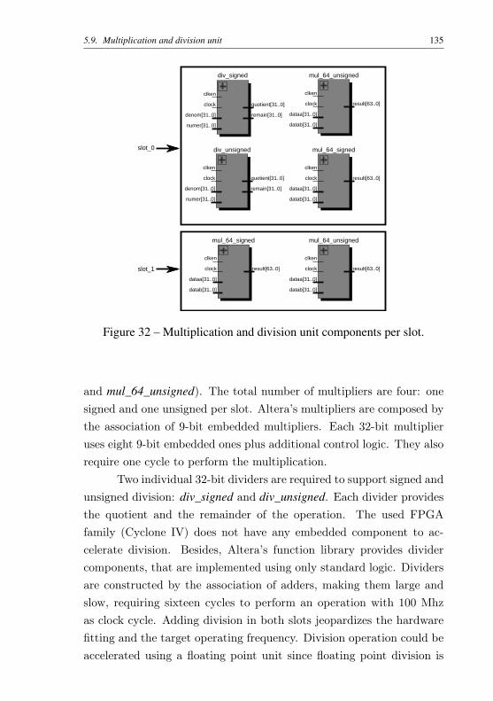
5.9. Multiplication and division unit 135
div_signed
clken
clock
denom[31..0]
numer[31..0]
quotient[31..0]
remain[31..0]
div_unsigned
clken
clock
denom[31..0]
numer[31..0]
quotient[31..0]
remain[31..0]
mul_64_unsigned
clken
clock
dataa[31..0]
datab[31..0]
result[63..0]
mul_64_signed
clken
clock
dataa[31..0]
datab[31..0]
result[63..0]
slot_0
mul_64_unsigned
clken
clock
dataa[31..0]
datab[31..0]
result[63..0]
mul_64_signed
clken
clock
dataa[31..0]
datab[31..0]
result[63..0]slot_1
Figure 32 – Multiplication and division unit components per slot.
and mul_64_unsigned). The total number of multipliers are four: onesigned and one unsigned per slot. Altera’s multipliers are composed bythe association of 9-bit embedded multipliers. Each 32-bit multiplieruses eight 9-bit embedded ones plus additional control logic. They alsorequire one cycle to perform the multiplication.
Two individual 32-bit dividers are required to support signed andunsigned division: div_signed and div_unsigned. Each divider providesthe quotient and the remainder of the operation. The used FPGAfamily (Cyclone IV) does not have any embedded component to ac-celerate division. Besides, Altera’s function library provides dividercomponents, that are implemented using only standard logic. Dividersare constructed by the association of adders, making them large andslow, requiring sixteen cycles to perform an operation with 100 Mhzas clock cycle. Adding division in both slots jeopardizes the hardwarefitting and the target operating frequency. Division operation could beaccelerated using a floating point unit since floating point division is
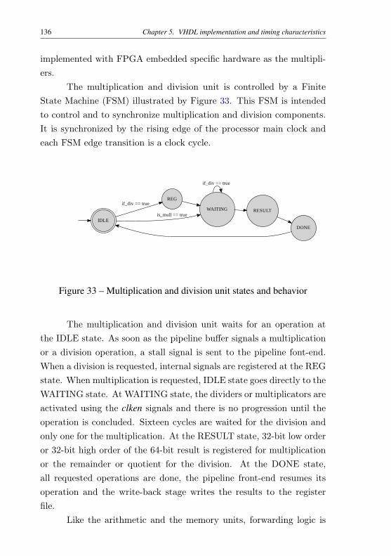
136 Chapter 5. VHDL implementation and timing characteristics
implemented with FPGA embedded specific hardware as the multipli-ers.
The multiplication and division unit is controlled by a FiniteState Machine (FSM) illustrated by Figure 33. This FSM is intendedto control and to synchronize multiplication and division components.It is synchronized by the rising edge of the processor main clock andeach FSM edge transition is a clock cycle.
IDLE
REGif_div == true
WAITINGis_mull == true
if_div == true
RESULT
DONE
Figure 33 – Multiplication and division unit states and behavior
The multiplication and division unit waits for an operation atthe IDLE state. As soon as the pipeline buffer signals a multiplicationor a division operation, a stall signal is sent to the pipeline font-end.When a division is requested, internal signals are registered at the REGstate. When multiplication is requested, IDLE state goes directly to theWAITING state. At WAITING state, the dividers or multiplicators areactivated using the clken signals and there is no progression until theoperation is concluded. Sixteen cycles are waited for the division andonly one for the multiplication. At the RESULT state, 32-bit low orderor 32-bit high order of the 64-bit result is registered for multiplicationor the remainder or quotient for the division. At the DONE state,all requested operations are done, the pipeline front-end resumes itsoperation and the write-back stage writes the results to the registerfile.
Like the arithmetic and the memory units, forwarding logic is
5.10. Timing characteristics and FPGA resource utilization 137
necessary as well. 9-input multiplexers are placed before dividers andmultiplicators inputs and their selection logic is similar to the previ-ously described Algorithm 2.
5.10 TIMING CHARACTERISTICS AND FPGA RESOURCE UTI-LIZATION
The FPGA resource utilization is shown in Table 20 with a clockspeed of 100MHz. The execution stage length description for eachinstruction type is shown in Table 21.
We can summaries the timing information required for the WCETanalyzer as follows:
∙ Cycle time: 10ns
∙ Cache miss: 15 cycles.
∙ Interlock latency: 1 cycle, only between arithmetic compares andconditional branches.
∙ Execution stage latencies: Table 21.
∙ Control-flow latencies:
– Not taken branch: no latency.
– Taken branch: 4 cycles.
– Call, goto: 4 cycles.
– Predicted taken branch: 1 cycle.
– Misspredicted branch: 6 cycles.
5.11 SUMMARY
The instruction cache memory was implemented in the FPGAusing internal RAM blocks. The instruction cache has 32 lines with256 bits per line forming a 1kb direct-mapped cache memory.
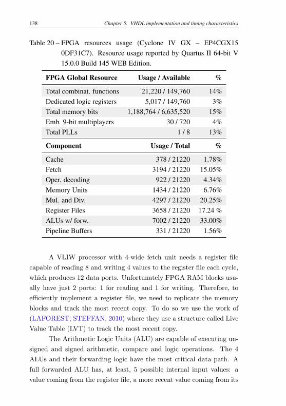
138 Chapter 5. VHDL implementation and timing characteristics
Table 20 – FPGA resources usage (Cyclone IV GX – EP4CGX150DF31C7). Resource usage reported by Quartus II 64-bit V15.0.0 Build 145 WEB Edition.
FPGA Global Resource Usage / Available %
Total combinat. functions 21,220 / 149,760 14%Dedicated logic registers 5,017 / 149,760 3%Total memory bits 1,188,764 / 6,635,520 15%Emb. 9-bit multiplayers 30 / 720 4%Total PLLs 1 / 8 13%
Component Usage / Total %
Cache 378 / 21220 1.78%Fetch 3194 / 21220 15.05%Oper. decoding 922 / 21220 4.34%Memory Units 1434 / 21220 6.76%Mul. and Div. 4297 / 21220 20.25%Register Files 3658 / 21220 17.24 %ALUs w/ forw. 7002 / 21220 33.00%Pipeline Buffers 331 / 21220 1.56%
A VLIW processor with 4-wide fetch unit needs a register filecapable of reading 8 and writing 4 values to the register file each cycle,which produces 12 data ports. Unfortunately FPGA RAM blocks usu-ally have just 2 ports: 1 for reading and 1 for writing. Therefore, toefficiently implement a register file, we need to replicate the memoryblocks and track the most recent copy. To do so we use the work of(LAFOREST; STEFFAN, 2010) where they use a structure called LiveValue Table (LVT) to track the most recent copy.
The Arithmetic Logic Units (ALU) are capable of executing un-signed and signed arithmetic, compare and logic operations. The 4ALUs and their forwarding logic have the most critical data path. Afull forwarded ALU has, at least, 5 possible internal input values: avalue coming from the register file, a more recent value coming from its
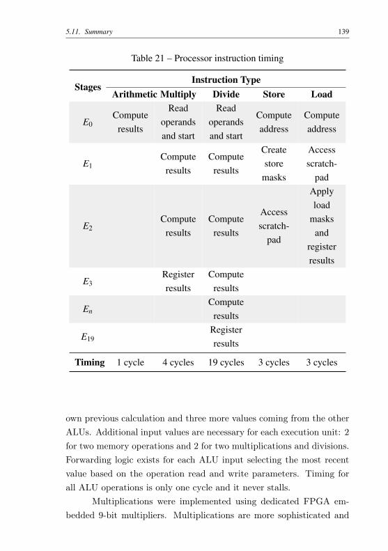
5.11. Summary 139
Table 21 – Processor instruction timing
StagesInstruction Type
Arithmetic Multiply Divide Store Load
E0Compute
results
Readoperandsand start
Readoperandsand start
Computeaddress
Computeaddress
E1Compute
resultsCompute
results
Createstore
masks
Accessscratch-
pad
E2Compute
resultsCompute
results
Accessscratch-
pad
Applyload
masksand
registerresults
E3Registerresults
Computeresults
EnCompute
results
E19Registerresults
Timing 1 cycle 4 cycles 19 cycles 3 cycles 3 cycles
own previous calculation and three more values coming from the otherALUs. Additional input values are necessary for each execution unit: 2for two memory operations and 2 for two multiplications and divisions.Forwarding logic exists for each ALU input selecting the most recentvalue based on the operation read and write parameters. Timing forall ALU operations is only one cycle and it never stalls.
Multiplications were implemented using dedicated FPGA em-bedded 9-bit multipliers. Multiplications are more sophisticated and
140 Chapter 5. VHDL implementation and timing characteristics
they need 4 stages to complete. Considering the current implementingtechnology, the number of substages is equal to the number of cycles. Adivision specialized VHDL block uses only combination logic. A singledivision requires 19 cycles to target 100Mhz and it is a very large com-ponent. To implement one hardware signed and one unsigned divisionwe need as much logic cells as half of the entire arithmetic unit (4 ALUwith all forwarding logic).
The Load/Store unit accesses only the scratchpad memory. Dataaccess from other memories should be done via DMA operation but thisis not covered in this thesis. A real-time deterministic DRAM controlleris described in the work of (REINEKE et al., 2011). The instructionmemory was implemented using internal FPGA memory with 2 readports, one for cache access and one DMA unit. The Scratchpad alsoused internal FPGA memory. Both scratchpad and SDRAM operateat 100Mhz.
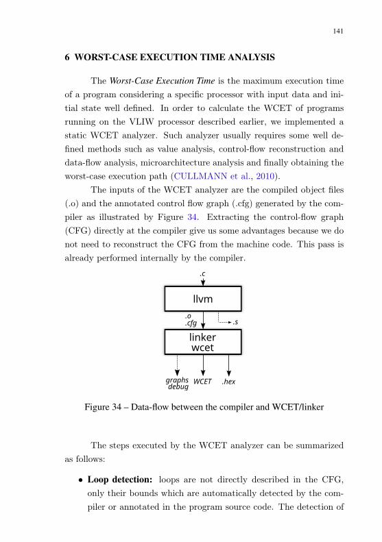
141
6 WORST-CASE EXECUTION TIME ANALYSIS
The Worst-Case Execution Time is the maximum execution timeof a program considering a specific processor with input data and ini-tial state well defined. In order to calculate the WCET of programsrunning on the VLIW processor described earlier, we implemented astatic WCET analyzer. Such analyzer usually requires some well de-fined methods such as value analysis, control-flow reconstruction anddata-flow analysis, microarchitecture analysis and finally obtaining theworst-case execution path (CULLMANN et al., 2010).
The inputs of the WCET analyzer are the compiled object files(.o) and the annotated control flow graph (.cfg) generated by the com-piler as illustrated by Figure 34. Extracting the control-flow graph(CFG) directly at the compiler give us some advantages because we donot need to reconstruct the CFG from the machine code. This pass isalready performed internally by the compiler.
llvm
linkerwcet
.o.s.cfg
.c
.hexWCETgraphsdebug
Figure 34 – Data-flow between the compiler and WCET/linker
The steps executed by the WCET analyzer can be summarizedas follows:
∙ Loop detection: loops are not directly described in the CFG,only their bounds which are automatically detected by the com-piler or annotated in the program source code. The detection of
142 Chapter 6. Worst-case Execution time analysis
loops uses Tarjan’s algorithm (LENGAUER; TARJAN, 1979) foridentifying strongly connected components in graphs.
∙ Instruction cache analysis: analysis for classification of cacheaccesses in always miss, always hit, first miss and conflict.
∙ Pipeline modeling: This pass models the VLIW pipeline behaviorcalculating the basic block times, disregarding any cache effects.
∙ Worst-case path search: This phase searches for the worst-casepath and its respective computation time (WCET), consideringthe previous analyses. We used Implicit Path Enumeration Tech-nique – IPET (LI; MALIK, 1995), which produces an optimalsolution, for this purpose.
Since the proposed architecture does not suffer from timing anoma-lies, we can conduct each analysis in isolation and combine the resultsat the path search phase.
Like most WCET analyzers, the implemented one is context sen-sitive. The analyzer considers the paths by which each node of the CFGcan be reached, and computes the behavior of cache and executions foreach node in each of these contexts. For example, loops may have a dif-ferent execution time for the first iteration, when instructions must beloaded in the cache. This behavior can be extracted by cache analysis,which is the subject of the next section.
6.1 BASIC CONCEPTS
Programs need to be represented mathematically to performstatic analysis. They are composed by a control flow graph, basicblocks, loops and paths. Aho et al. (2011) defined each one as follows:
Definition 1. (Basic Block – bb) A basic block is a maximal sequenceof instructions, which can be reached only by its first instruction and theonly way out is its last instruction.
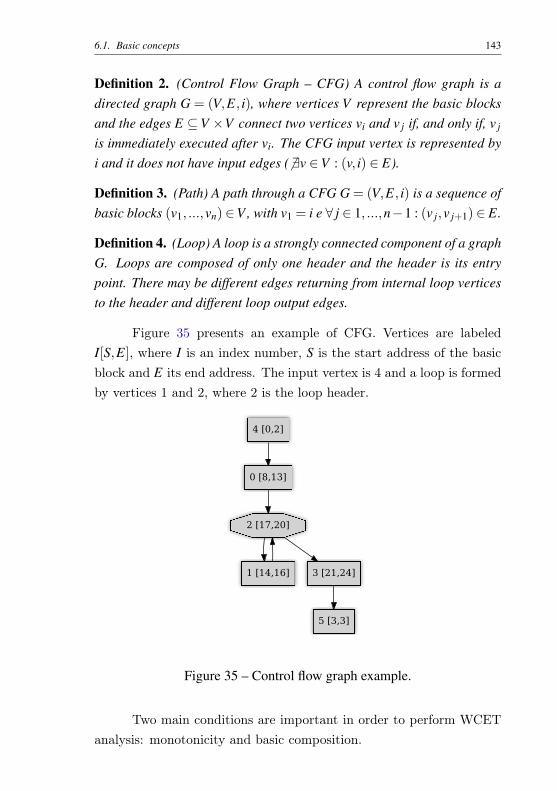
6.1. Basic concepts 143
Definition 2. (Control Flow Graph – CFG) A control flow graph is adirected graph G = (V,E, i), where vertices V represent the basic blocksand the edges E ⊆V ×V connect two vertices vi and v j if, and only if, v j
is immediately executed after vi. The CFG input vertex is represented byi and it does not have input edges (̸ ∃v ∈V : (v, i) ∈ E).
Definition 3. (Path) A path through a CFG G = (V,E, i) is a sequence ofbasic blocks (v1, ...,vn)∈V , with v1 = i e ∀ j ∈ 1, ...,n−1 : (v j,v j+1)∈ E.
Definition 4. (Loop) A loop is a strongly connected component of a graphG. Loops are composed of only one header and the header is its entrypoint. There may be different edges returning from internal loop verticesto the header and different loop output edges.
Figure 35 presents an example of CFG. Vertices are labeledI[S,E], where I is an index number, S is the start address of the basicblock and E its end address. The input vertex is 4 and a loop is formedby vertices 1 and 2, where 2 is the loop header.
0 [8,13]
2 [17,20]
1 [14,16] 3 [21,24]
5 [3,3]
4 [0,2]
Figure 35 – Control flow graph example.
Two main conditions are important in order to perform WCETanalysis: monotonicity and basic composition.
144 Chapter 6. Worst-case Execution time analysis
Monotonicity means that an instruction with a higher latencynecessarily maintains or increases the time of a sequence of instructionsunder analysis. A higher latency instruction should never decrease theoverall execution time because the local worst case should not diminishthe global worst case. In the case of temporal anomalies, this assump-tion does not hold.
Basic composition means that the WCET values of sub-paths canbe safely composed when calculating the overall WCET. Like mono-tonicity, the basic composition property is also lost in the presence oftemporal anomalies.
The processor described in this thesis does not present timinganomalies and so we can assume monotonicity and basic composition.The purpose of the next analyses is to obtain the individual basic blocktiming which it can be expressed by:
tbb = tp +nc.tc +nm.tm (6.1)
Symbol tp is the basic block pipeline timing considering all mul-tistage operations and nc.tc is the number of cache misses multiplied bythe cache penalty. The processor only accesses the scratchpad mem-ory and this is already considered as a multistage operation during thepipeline analysis. An eventual memory penalty (as a DMA transfer)could be modeled by nm.tm where nm is the number of memory accessesand tm is the memory access timing.
After the timings of all basic blocks are estimated, the programexecution time is calculated by:
ob j = maximize ∑∀bbi
xi× ti (6.2)
Symbol xi is the number of times basic block bbi is executed andti is the worst execution time of bbi.
6.2. Instruction cache analysis 145
6.2 INSTRUCTION CACHE ANALYSIS
Cache memories are necessary to minimize the gap between pro-cessor and memory performances. Usually, main memory has a clockthat is slower than the processor, so a fast cache is placed betweenthem where most recent data is stored, promoting faster access. Weuse a direct-mapped instruction cache memory, so some sort of analy-sis is necessary to model cache misses during WCET analysis. Usuallycache analysis is performed using abstract interpretation as describedin (ALT et al., 1996) but here we used traditional data flow analysis tocompute cache states. Similar analyses are also used in (MUELLER;WHALLEY, 1995) and (LEE et al., 1998).
A cache memory is characterized by its capacity, line size andassociativity.
Definition 5. (Capacity) Capacity is the cache’s total number of bytes.
Definition 6. (Line or block size) Line size is the quantity of bytes trans-ferred from memory to cache when a cache miss occurs. A cache shouldhave n = capacity
line. size lines.
Definition 7. (Associativity) It consists of the mapping of various mainmemory addresses to cache lines. A direct-mapped cache has unitaryassociativity, where a main memory specific address is always mappedto the same cache line. If associativity is 2, a main memory address ismapped to 2 different cache lines. When associativity is not unitary somesort of replacement policy must exist to decide which line will have dataeviction. The relation n
assoc. defines the number of sets of a cache.
In the context of this work, we will focus only on unitary asso-ciativity (direct mapping) when one memory block can reside only in aspecific cache line. This feature does not impose a restriction upon theanalysis, but is related to the used direct-mapping configuration in thehardware. A direct-mapping cache memory is formed by a sequence oflines L = l1, l2, ln... which store a set of memory blocks M = m1,m2...ms.A memory block m with address addr is stored in line li following Equa-
146 Chapter 6. Worst-case Execution time analysis
tion 6.3. The operator % represents the modulus or remainder of thedivision.
li = addr(m) % n (6.3)
Regarding the presence of the existence of a particular instruc-tion in the cache, we define:
Definition 8. An instruction could be in the cache if: 1) there was atransition sequence in which the block corresponding to the instructionmemory had been referenced in previous basic blocks; 2) this memoryblock is referenced previously in the same basic block.
Definition 9. (Abstract state) An abstract state of the cache of a basicblock is the subset of all memory blocks that can be cached before execut-ing the basic block.
Definition 10. (Reachable abstract state) A reachable abstract state isthe subset of all memory blocks that can be reached by CFG transitions.
Definition 11. (Effective abstract state) An effective abstract state of abasic block is a subset of all memory blocks that can be reached by con-sidering all the CFG paths to the basic block in analysis.
6.2.1 Reachable and effective abstract state
We can construct the reachable abstract state where we can mapall memory blocks accessed by every basic block. This analysis uses thesame principles of reaching definitions in traditional data flow analysisand it follows Algorithm 3.
Figure 36 shows an example of data flow applied to cache anal-ysis. The abstract reachable state (RMBbb(cl) = data) is beside eachoutput edge. bb is the basic block number, cl is the cache line anddata represents an identifier of the memory data, the memory addressindex. Figure 36 also shows which cache line is accessed by a basicblock and its memory address index inside the nodes (l0 = 0 for ba-sic block 0 and l1 = 1 for basic block 4). It is very easy to know the
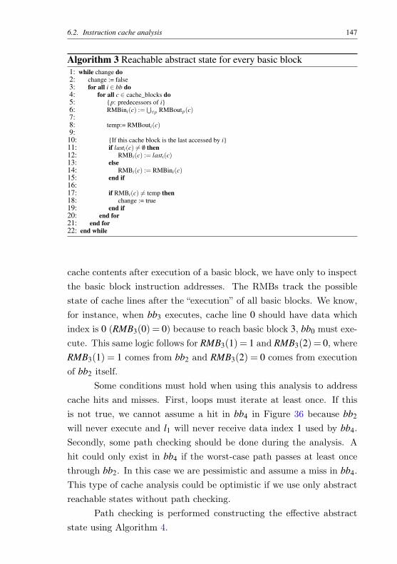
6.2. Instruction cache analysis 147
Algorithm 3 Reachable abstract state for every basic block1: while change do2: change := false3: for all i ∈ bb do4: for all c ∈ cache_blocks do5: {p: predecessors of i}6: RMBini(c) :=
⋃∀p RMBoutp(c)
7:8: temp:= RMBouti(c)9:
10: {If this cache block is the last accessed by i}11: if lasti(c) ̸= /0 then12: RMBi(c) := lasti(c)13: else14: RMBi(c) := RMBini(c)15: end if16:17: if RMBi(c) ̸= temp then18: change := true19: end if20: end for21: end for22: end while
cache contents after execution of a basic block, we have only to inspectthe basic block instruction addresses. The RMBs track the possiblestate of cache lines after the “execution” of all basic blocks. We know,for instance, when bb3 executes, cache line 0 should have data whichindex is 0 (RMB3(0) = 0) because to reach basic block 3, bb0 must exe-cute. This same logic follows for RMB3(1) = 1 and RMB3(2) = 0, whereRMB3(1) = 1 comes from bb2 and RMB3(2) = 0 comes from executionof bb2 itself.
Some conditions must hold when using this analysis to addresscache hits and misses. First, loops must iterate at least once. If thisis not true, we cannot assume a hit in bb4 in Figure 36 because bb2
will never execute and l1 will never receive data index 1 used by bb4.Secondly, some path checking should be done during the analysis. Ahit could only exist in bb4 if the worst-case path passes at least oncethrough bb2. In this case we are pessimistic and assume a miss in bb4.This type of cache analysis could be optimistic if we use only abstractreachable states without path checking.
Path checking is performed constructing the effective abstractstate using Algorithm 4.
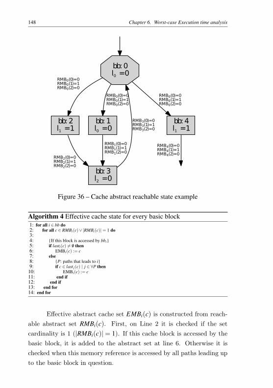
148 Chapter 6. Worst-case Execution time analysis
bb: 0l0 = 0
bb: 1l0 = 0
RMB0(0)= 0RMB0(1)= 1RMB0(2)= 0
bb: 2l1 = 1
RMB0(0)= 0RMB0(1)= 1RMB0(2)= 0
bb: 4l1 = 1
RMB0(0)= 0RMB0(1)= 1RMB0(2)= 0
bb: 3l2 = 0
RMB1(0)= 0RMB1(1)= 1RMB1(2)= 0
RMB2(0)= 0RMB2(1)= 1RMB2(2)= 0
RMB3(0)= 0RMB3(1)= 1RMB3(2)= 0
RMB4(0)= 0RMB4(1)= 1RMB4(2)= 0
Figure 36 – Cache abstract reachable state example
Algorithm 4 Effective cache state for every basic block1: for all i ∈ bb do2: for all c ∈ RMBi(c)∨|RMBi(c)|= 1 do3:4: {If this block is accessed by bbi}5: if lasti(c) ̸= /0 then6: EMBi(c) := c7: else8: {P: paths that leads to i}9: if c ∈ last j(c) | j ∈ ∀P then
10: EMBi(c) := c11: end if12: end if13: end for14: end for
Effective abstract cache set EMBi(c) is constructed from reach-able abstract set RMBi(c). First, on Line 2 it is checked if the setcardinality is 1 (|RMBi(c)|= 1). If this cache block is accessed by thebasic block, it is added to the abstract set at line 6. Otherwise it ischecked when this memory reference is accessed by all paths leading upto the basic block in question.
6.2. Instruction cache analysis 149
Considering the example in Figure 36 and the basic block 4,the algorithm has the following execution in the construction of theeffective abstract state for cache line 1 of basic block 0 (EMB0(1)):
∙ if vertex 0 accessed l1 = 1, we could terminate and it will beclassified as a cache hit;
∙ following vertex 0, we check 3, where there is no access;
∙ following vertex 3, we check 2. In this vertex, l1 = 1 is accessedand this path search is ended;
∙ following vertex 3, we check 1. There is not a l1 = 1 access andwe continue;
∙ following vertex 1, we check 0. Vertex 0 was already visited. Wecan conclude that there is a path where l1 = 1 is not referenced;
∙ l1 = 1 does not belong to the effective abstract state of basic block0 and therefore there is a cache miss in basic block 4.
6.2.2 Cache accesses classification
We classify all program instructions in “always miss”, “alwayshit”, “first miss” and “conflict” after the data flow analysis in conjunctionwith path checking – reachable and effective abstract state.
Definition 12. (A_MISS) There is a cache fault every time this instructionis executed – always miss.
A_MISS classification occurs in compulsory or capacity faults.For example, a compulsory miss occurs in bb0 in Figure 36 since the firstinstruction of the program is not in the cache memory at the beginningof the program execution. A_Miss is also the correct classification forthe instruction of bb4, since l1 = 1 does not exist in the effective abstractstate of bb0 (predecessor of bb4).
Definition 13. (A_HIT) There is a cache hit every time this instruction isexecuted – always hit.
150 Chapter 6. Worst-case Execution time analysis
A_HIT is the class for instructions where: 1) they are not thebasic block first instruction or the first instruction of a cache line; 2)they are in the cache effective state. In the case of Figure 36, allinstructions of the bb1 can be classified as hits because their cache linewill always be previously accessed by the bb0.
Definition 14. (F_MISS) This classification is related to loops. There isa cache miss only at the first iteration of the loop – first miss;
In the case of F_MISS, if a loop iterates 100 times, there is acache miss only at the first iteration. For the other 99 iterations, thereare cache hits. This classification occurs in the bb2 of Figure 36 forl1 = 1 since it is not accessed by any predecessor except itself.
Definition 15. (CONFLICT) This classification occurs when there aremultiple reachable paths to a particular basic block and each of thesepaths has a different effective cache state, which may cause faults ormisses depending on the path flow.
CONFLICT occurs, for example, in bb3 of Figure 37. If theexecution flow is 0→ 2→ 3, there is a cache hit since l1 = 1 is accessedin bb2; if the execution flow is 0→ 1→ 3, there is a cache miss sincethere are no references to l1 = 1 in predecessor basic blocks.
After instruction classification, we can count the number of faults(A_MISS) that impact directly on the basic block time. The classesF_MISS and CONFLICT are used during the path analysis to deter-mine the program flow that maximizes the execution time.
6.3 PIPELINE MODELING
The objective of this analysis is to determine the execution timeof instructions and basic blocks when executed on the processor pipeline.This analysis does not consider hardware elements like instruction cache.
Pipelined processors, the execution time of a single instructionin cycles will be at least to the number of pipeline stages. However, thistime may be higher if any hazard occurs involving data dependencies
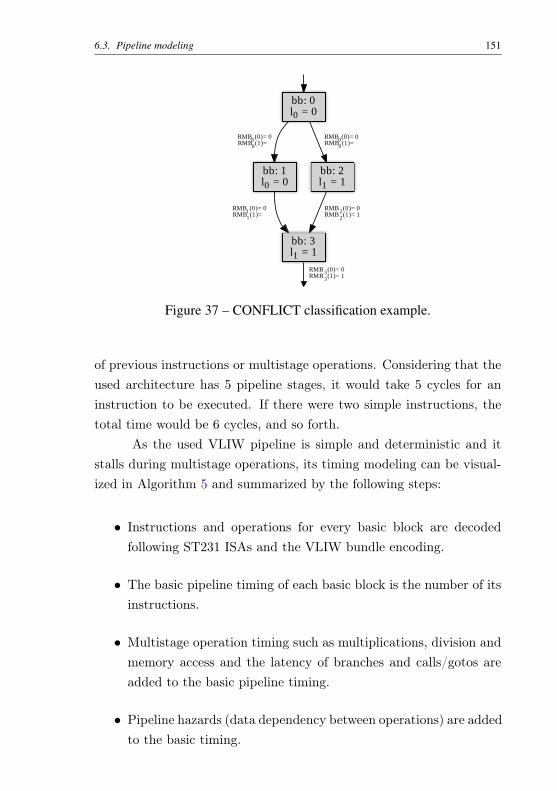
6.3. Pipeline modeling 151
bb: 0l0 = 0
bb: 1l0 = 0
RMB0(0)= 0RMB0(1)=
bb: 2l1 = 1
bb: 3l1 = 1
RMB1(0)= 0RMB1(1)=
RMB 2(0)= 0RMB 2(1)= 1
RMB 3(0)= 0RMB 3(1)= 1
RMB0(0)= 0RMB0(1)=
Figure 37 – CONFLICT classification example.
of previous instructions or multistage operations. Considering that theused architecture has 5 pipeline stages, it would take 5 cycles for aninstruction to be executed. If there were two simple instructions, thetotal time would be 6 cycles, and so forth.
As the used VLIW pipeline is simple and deterministic and itstalls during multistage operations, its timing modeling can be visual-ized in Algorithm 5 and summarized by the following steps:
∙ Instructions and operations for every basic block are decodedfollowing ST231 ISAs and the VLIW bundle encoding.
∙ The basic pipeline timing of each basic block is the number of itsinstructions.
∙ Multistage operation timing such as multiplications, division andmemory access and the latency of branches and calls/gotos areadded to the basic pipeline timing.
∙ Pipeline hazards (data dependency between operations) are addedto the basic timing.
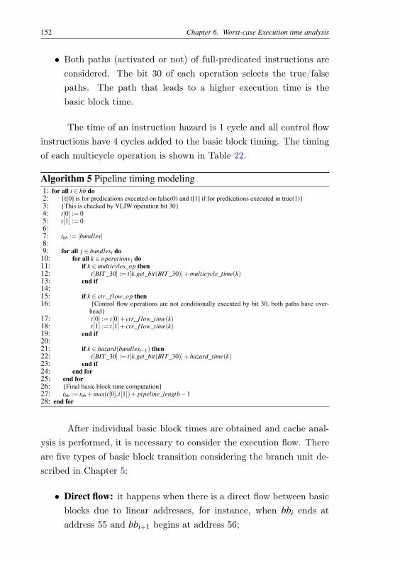
152 Chapter 6. Worst-case Execution time analysis
∙ Both paths (activated or not) of full-predicated instructions areconsidered. The bit 30 of each operation selects the true/falsepaths. The path that leads to a higher execution time is thebasic block time.
The time of an instruction hazard is 1 cycle and all control flowinstructions have 4 cycles added to the basic block timing. The timingof each multicycle operation is shown in Table 22.
Algorithm 5 Pipeline timing modeling1: for all i ∈ bb do2: {t[0] is for predications executed on false(0) and t[1] if for predications executed in true(1)}3: {This is checked by VLIW operation bit 30}4: t[0] := 05: t[1] := 06:7: tbb := |bundles|8:9: for all j ∈ bundlesi do
10: for all k ∈ operations j do11: if k ∈ multicyles_op then12: t[BIT _30] := t[k.get_bit(BIT _30)]+multicycle_time(k)13: end if14:15: if k ∈ ctr_ f low_op then16: {Control flow operations are not conditionally executed by bit 30, both paths have over-
head}17: t[0] := t[0]+ ctr_ f low_time(k)18: t[1] := t[1]+ ctr_ f low_time(k)19: end if20:21: if k ∈ hazard(bundlesi−1) then22: t[BIT _30] := t[k.get_bit(BIT _30)]+hazard_time(k)23: end if24: end for25: end for26: {Final basic block time computation}27: tbb := tbb +max(t[0], t[1])+ pipeline_length−128: end for
After individual basic block times are obtained and cache anal-ysis is performed, it is necessary to consider the execution flow. Thereare five types of basic block transition considering the branch unit de-scribed in Chapter 5:
∙ Direct flow: it happens when there is a direct flow between basicblocks due to linear addresses, for instance, when bbi ends ataddress 55 and bbi+1 begins at address 56;
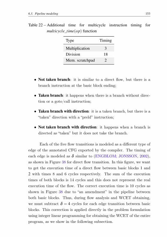
6.3. Pipeline modeling 153
Table 22 – Additional time for multicycle instruction timing formulticycle_time(op) function
Type Timing
Multiplication 3Division 18Mem. scratchpad 2
∙ Not taken branch: it is similar to a direct flow, but there is abranch instruction at the basic block ending;
∙ Taken branch: it happens when there is a branch without direc-tion or a goto/call instruction;
∙ Taken branch with direction: it is a taken branch, but there is a“taken” direction with a “preld” instruction;
∙ Not taken branch with direction: it happens when a branch isdirected as “taken” but it does not take the branch.
Each of the five flow transitions is modeled as a different type ofedge of the annotated CFG exported by the compiler. The timing ofeach edge is modeled as δ similar to (ENGBLOM; JONSSON, 2002),as shown in Figure 38 for direct flow transition. In this figure, we wantto get the execution time of a direct flow between basic blocks 1 and2 with times 8 and 6 cycles respectively. The sum of the executiontimes of both blocks is 14 cycles and this does not represent the realexecution time of the flow. The correct execution time is 10 cycles asshown in Figure 38 due to “an amendment” in the pipeline betweenboth basic blocks. Thus, during flow analysis and WCET obtaining,we must subtract δ = 4 cycles for each edge transition between basicblocks. This correction is applied directly in the problem formulationusing integer linear programming for obtaining the WCET of the entireprogram, as we show in the following subsection.
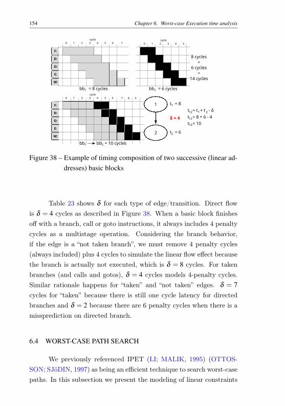
154 Chapter 6. Worst-case Execution time analysis
cycle
F:
0 1 2 3 4 5 6
D:
O:
E:
W:
7cycle
0 1 2 3 4 5
bb1 = 8 cycles bb2 = 6 cyclescycle
0 1 2 3 4 5 6 7 8 9
F:
D:
O:
E:
W:
bb1 bb2 = 10 cycles
8 cycles+
6 cycles=
14 cycles
1
2
t = 81
t = 62
δ = 4
t = t + t - δ t = 8 + 6 - 4t = 10
1 212
12
12
Figure 38 – Example of timing composition of two successive (linear ad-dresses) basic blocks
Table 23 shows δ for each type of edge/transition. Direct flowis δ = 4 cycles as described in Figure 38. When a basic block finishesoff with a branch, call or goto instructions, it always includes 4 penaltycycles as a multistage operation. Considering the branch behavior,if the edge is a “not taken branch”, we must remove 4 penalty cycles(always included) plus 4 cycles to simulate the linear flow effect becausethe branch is actually not executed, which is δ = 8 cycles. For takenbranches (and calls and gotos), δ = 4 cycles models 4-penalty cycles.Similar rationale happens for “taken” and “not taken” edges. δ = 7cycles for “taken” because there is still one cycle latency for directedbranches and δ = 2 because there are 6 penalty cycles when there is amissprediction on directed branch.
6.4 WORST-CASE PATH SEARCH
We previously referenced IPET (LI; MALIK, 1995) (OTTOS-SON; SJöDIN, 1997) as being an efficient technique to search worst-casepaths. In this subsection we present the modeling of linear constraints
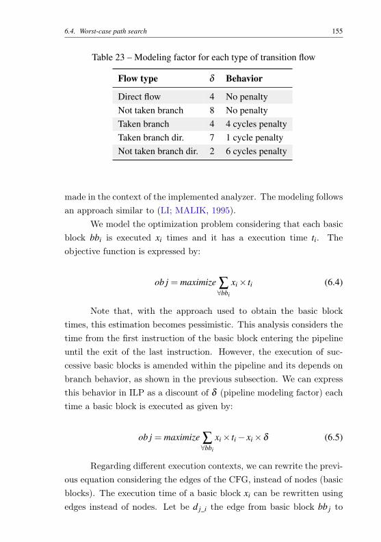
6.4. Worst-case path search 155
Table 23 – Modeling factor for each type of transition flow
Flow type δ Behavior
Direct flow 4 No penaltyNot taken branch 8 No penaltyTaken branch 4 4 cycles penaltyTaken branch dir. 7 1 cycle penaltyNot taken branch dir. 2 6 cycles penalty
made in the context of the implemented analyzer. The modeling followsan approach similar to (LI; MALIK, 1995).
We model the optimization problem considering that each basicblock bbi is executed xi times and it has a execution time ti. Theobjective function is expressed by:
ob j = maximize ∑∀bbi
xi× ti (6.4)
Note that, with the approach used to obtain the basic blocktimes, this estimation becomes pessimistic. This analysis considers thetime from the first instruction of the basic block entering the pipelineuntil the exit of the last instruction. However, the execution of suc-cessive basic blocks is amended within the pipeline and its depends onbranch behavior, as shown in the previous subsection. We can expressthis behavior in ILP as a discount of δ (pipeline modeling factor) eachtime a basic block is executed as given by:
ob j = maximize ∑∀bbi
xi× ti− xi×δ (6.5)
Regarding different execution contexts, we can rewrite the previ-ous equation considering the edges of the CFG, instead of nodes (basicblocks). The execution time of a basic block xi can be rewritten usingedges instead of nodes. Let be d j_i the edge from basic block bb j to
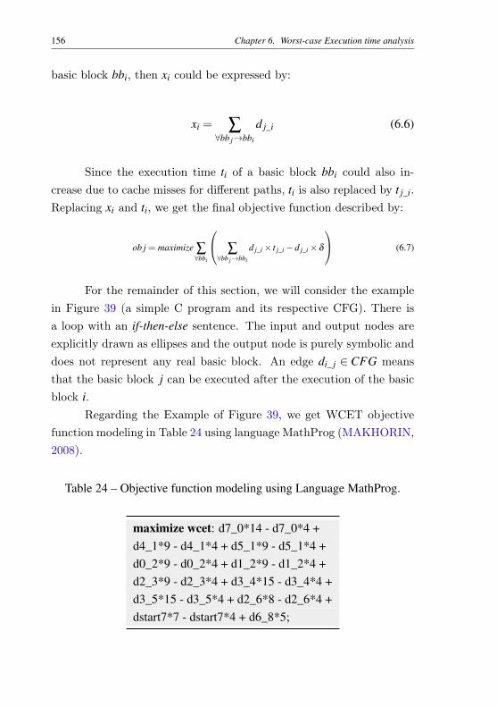
156 Chapter 6. Worst-case Execution time analysis
basic block bbi, then xi could be expressed by:
xi = ∑∀bb j→bbi
d j_i (6.6)
Since the execution time ti of a basic block bbi could also in-crease due to cache misses for different paths, ti is also replaced by t j_i.Replacing xi and ti, we get the final objective function described by:
ob j = maximize ∑∀bbi
∑∀bb j→bbi
d j_i× t j_i−d j_i×δ
(6.7)
For the remainder of this section, we will consider the examplein Figure 39 (a simple C program and its respective CFG). There isa loop with an if-then-else sentence. The input and output nodes areexplicitly drawn as ellipses and the output node is purely symbolic anddoes not represent any real basic block. An edge di_ j ∈ CFG meansthat the basic block j can be executed after the execution of the basicblock i.
Regarding the Example of Figure 39, we get WCET objectivefunction modeling in Table 24 using language MathProg (MAKHORIN,2008).
Table 24 – Objective function modeling using Language MathProg.
maximize wcet: d7_0*14 - d7_0*4 +d4_1*9 - d4_1*4 + d5_1*9 - d5_1*4 +d0_2*9 - d0_2*4 + d1_2*9 - d1_2*4 +d2_3*9 - d2_3*4 + d3_4*15 - d3_4*4 +d3_5*15 - d3_5*4 + d2_6*8 - d2_6*4 +dstart7*7 - dstart7*4 + d6_8*5;
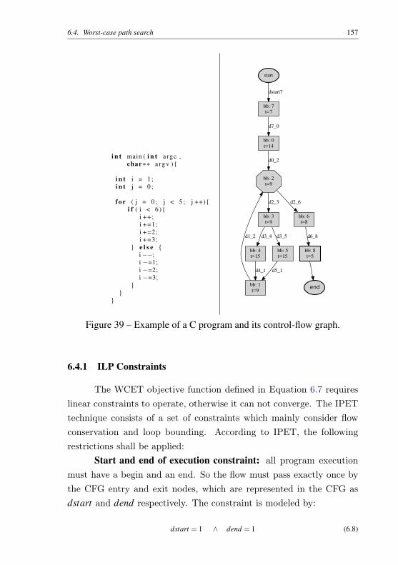
6.4. Worst-case path search 157
i n t main ( i n t argc ,char** a rgv ) {
i n t i = 1 ;i n t j = 0 ;
f o r ( j = 0 ; j < 5 ; j ++){i f ( i < 6 ){
i ++;i +=1;i +=2;i +=3;
} e l s e {i−−;i −=1;i −=2;i −=3;
}}
}
start
bb: 7t=7
dstart7
bb: 0t=14
bb: 2t=9
d0_2
bb: 1t=9
d1_2
bb: 3t=9
d2_3
bb: 6t=8
d2_6
bb: 4t=15
d3_4
bb: 5t=15
d3_5
d4_1 d5_1
bb: 8t=5
d6_8
d7_0
end
Figure 39 – Example of a C program and its control-flow graph.
6.4.1 ILP Constraints
The WCET objective function defined in Equation 6.7 requireslinear constraints to operate, otherwise it can not converge. The IPETtechnique consists of a set of constraints which mainly consider flowconservation and loop bounding. According to IPET, the followingrestrictions shall be applied:
Start and end of execution constraint: all program executionmust have a begin and an end. So the flow must pass exactly once bythe CFG entry and exit nodes, which are represented in the CFG asdstart and dend respectively. The constraint is modeled by:
dstart = 1 ∧ dend = 1 (6.8)
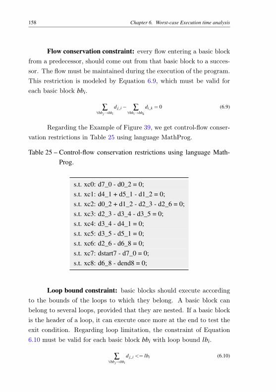
158 Chapter 6. Worst-case Execution time analysis
Flow conservation constraint: every flow entering a basic blockfrom a predecessor, should come out from that basic block to a succes-sor. The flow must be maintained during the execution of the program.This restriction is modeled by Equation 6.9, which must be valid foreach basic block bbi.
∑∀bb j→bbi
d j_i− ∑∀bbi→bbk
di_k = 0 (6.9)
Regarding the Example of Figure 39, we get control-flow conser-vation restrictions in Table 25 using language MathProg.
Table 25 – Control-flow conservation restrictions using language Math-Prog.
s.t. xc0: d7_0 - d0_2 = 0;s.t. xc1: d4_1 + d5_1 - d1_2 = 0;s.t. xc2: d0_2 + d1_2 - d2_3 - d2_6 = 0;s.t. xc3: d2_3 - d3_4 - d3_5 = 0;s.t. xc4: d3_4 - d4_1 = 0;s.t. xc5: d3_5 - d5_1 = 0;s.t. xc6: d2_6 - d6_8 = 0;s.t. xc7: dstart7 - d7_0 = 0;s.t. xc8: d6_8 - dend8 = 0;
Loop bound constraint: basic blocks should execute accordingto the bounds of the loops to which they belong. A basic block canbelong to several loops, provided that they are nested. If a basic blockis the header of a loop, it can execute once more at the end to test theexit condition. Regarding loop limitation, the constraint of Equation6.10 must be valid for each basic block bbi with loop bound lbi.
∑∀bb j→bbi
d j_i <= lbi (6.10)
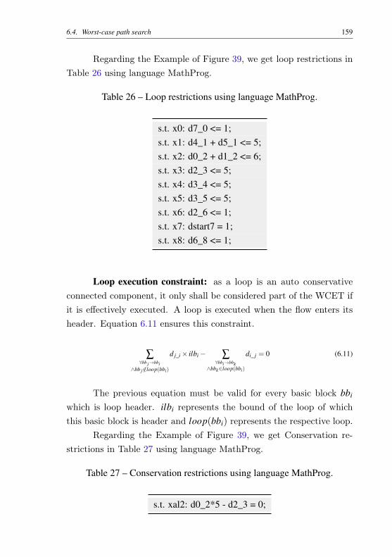
6.4. Worst-case path search 159
Regarding the Example of Figure 39, we get loop restrictions inTable 26 using language MathProg.
Table 26 – Loop restrictions using language MathProg.
s.t. x0: d7_0 <= 1;s.t. x1: d4_1 + d5_1 <= 5;s.t. x2: d0_2 + d1_2 <= 6;s.t. x3: d2_3 <= 5;s.t. x4: d3_4 <= 5;s.t. x5: d3_5 <= 5;s.t. x6: d2_6 <= 1;s.t. x7: dstart7 = 1;s.t. x8: d6_8 <= 1;
Loop execution constraint: as a loop is an auto conservativeconnected component, it only shall be considered part of the WCET ifit is effectively executed. A loop is executed when the flow enters itsheader. Equation 6.11 ensures this constraint.
∑∀bb j→bbi
∧bb j /∈loop(bbi)
d j_i× ilbi− ∑∀bbi→bbk
∧bbk∈loop(bbi)
di_ j = 0 (6.11)
The previous equation must be valid for every basic block bbi
which is loop header. ilbi represents the bound of the loop of whichthis basic block is header and loop(bbi) represents the respective loop.
Regarding the Example of Figure 39, we get Conservation re-strictions in Table 27 using language MathProg.
Table 27 – Conservation restrictions using language MathProg.
s.t. xal2: d0_2*5 - d2_3 = 0;
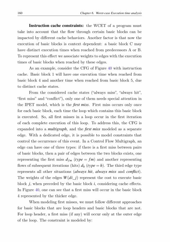
160 Chapter 6. Worst-case Execution time analysis
Instruction cache constraints: the WCET of a program musttake into account that the flow through certain basic blocks can beimpacted by different cache behaviors. Another factor is that now theexecution of basic blocks is context dependent: a basic block C mayhave distinct execution times when reached from predecessors A or B.To represent this effect we associate weights to edges with the executiontimes of basic blocks when reached by these edges.
As an example, consider the CFG of Figure 40 with instructioncache. Basic block 1 will have one execution time when reached frombasic block 4 and another time when reached from basic block 5, dueto distinct cache states.
From the considered cache states (“always miss”, “always hit”,“first miss” and “conflict”), only one of them needs special attention inthe IPET model, which is the first miss. First miss occurs only oncefor each basic block, each time the loop which contains this basic blockis executed. So, all first misses in a loop occur in the first iterationof each complete execution of this loop. To address this, the CFG isexpanded into a multigraph, and the first miss modeled as a separateedge. With a dedicated edge, it is possible to model constraints thatcontrol the occurrence of this event. In a Control Flow Multigraph, anedge can have one of three types: if there is a first miss between pairsof basic blocks, then a pair of edges between the two blocks exists, onerepresenting the first miss d f m (type = f m) and another representingflows of subsequent iterations (hits) dh (type = h). The third edge typerepresents all other situations (always hit, always miss and conflict).The weights of the edges W (di_ j) represent the cost to execute basicblock j, when preceded by the basic block i, considering cache effects.In Figure 40, one can see that a first miss will occur in the basic block4 represented by the thicker edge.
When modeling first misses, we must follow different approachesfor basic blocks that are loop headers and basic blocks that are not.For loop header, a first miss (if any) will occur only at the outer edgeof the loop. The constraint is modeled by:
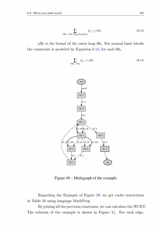
6.4. Worst-case path search 161
∑∀bb j→bbi∧bb j /∈loop(bbi)
d j_i ≤ elbi (6.12)
elbi is the bound of the outer loop bbi. For normal basic blocksthe constraint is modeled by Equation 6.13, for each bbi.
∑∀bb j→bbi
d j_i ≤ elbi (6.13)
start
bb: 7
dstart7
bb: 0
bb: 2
d0_2
bb: 1
d1_2
bb: 3
d2_3fmd2_3h
bb: 6
d2_6
bb: 4
d3_4fm d3_4h
bb: 5
d3_5h d3_5fm
d4_1 d5_1
bb: 8
d6_8
d7_0
end
Figure 40 – Multigraph of the example
Regarding the Example of Figure 39, we get cache restrictionsin Table 28 using language MathProg.
By joining all the previous constrains, we can calculate the WCET.The solution of the example is shown in Figure 41. For each edge,
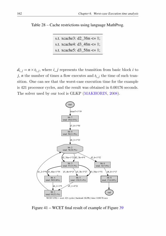
162 Chapter 6. Worst-case Execution time analysis
Table 28 – Cache restrictions using language MathProg.
s.t. xcache3: d2_3fm <= 1;s.t. xcache4: d3_4fm <= 1;s.t. xcache5: d3_5fm <= 1;
di_ j = n× ti_ j, where i_ j represents the transition from basic block i toj, n the number of times a flow executes and ti_ j the time of such tran-sition. One can see that the worst-case execution time for the exampleis 421 processor cycles, and the result was obtained in 0.00176 seconds.The solver used by our tool is GLKP (MAKHORIN, 2008).
WCET CFG > wcet: 421 cycles | backend: GLPK | time: 0.00176 secs
start
bb: 7total: 19(4.51%)
dstart7=1*19
bb: 0total: 50(11.9%)
bb: 2total: 78(18.5%)
d0_2=1*33
bb: 1total: 93(22.1%)
d1_2=5*9
bb: 3total: 57(13.5%)
d2_3fm=1*21 d2_3h=4*9
bb: 6total: 32(7.6%)
d2_6=1*32
bb: 4total: 39(9.26%)
d3_4fm=1*39 d3_4h=0*15
bb: 5total: 132(31.4%)
d3_5h=3*27 d3_5fm=1*51
d4_1=1*9 d5_1=4*21
bb: 8total: 17(4.04%)
d6_8=1*17
d7_0=1*50
end
Figure 41 – WCET final result of example of Figure 39
6.5. Summary 163
6.5 SUMMARY
This chapter presented techniques to perform the WCET analy-sis for the VLIW processor considered in this thesis. A tool consideringall described aspects was implemented in C++. Since we target per-formance enhancement on using VLIW machines for real-time systems,all evaluations performed were obtained through this WCET analysis.
In relation to static analysis, we can notice that it is a task thatdemands the union of numerous techniques such as data flow analy-sis (cache), path analysis (IPET) and modeling of internal processorcomponents. The more complex is the system in question, more com-plex are the techniques used. Nevertheless, it is very important thatthe system allows monotonicity and basic composition properties. Ifthese assumptions hold, we can increase the efficiency and precision ofa particular technique, such as cache analysis, and increase the over-all WCET analysis capabilities. Otherwise, the analysis will becomeincreasingly complex.

165
7 EVALUATION
In this chapter, we evaluate the impact of several architecturetechniques upon WCET performance. The main idea is to quantita-tively show WCET performance gains considering features like widerinstructions fetching, multiple memory operations, static branch pre-diction and predication.
To make WCET evaluations, we used the new code genera-tor back-end for LLVM (LATTNER; ADVE, 2004) and the describedWCET analyzer to compute the WCET of representative examples ofMälardalen WCET benchmarks (GUSTAFSSON et al., 2010). BothLLVM and the WCET framework are implemented in C++ and theirsource code are available upon request as well as the processor VHDLcode.
The Mälardalen WCET benchmarks are a set of programs thathave been assembled to make comparison between WCET tools. Anumber of WCET analysis tools have emerged in recent years and acomparison between these tools requires a common set of benchmarks.The typical evaluation metric is the accuracy of the WCET estimate,but of equal importance are other properties such as performance andthe ability to handle all code constructs found in real-time systems.The goal of the Mälardalen WCET benchmarks is to provide an easilyavailable, tested, and well documented common set of benchmarks inorder to enable comparative evaluations of different algorithms, meth-ods, and tools.
Table 29 shows a description of used benchmarks excluding thosewhich use library functions, floating-point calculations and recursion.Static data are allocated to scratchpad memory during processor bootprocess and this time is not included. Some benchmarks are so smallthat this may have a non-null impact on performance.
The performance of a program execution on a processor dependson the compiler capabilities for that specific processor. Besides seman-tics, a VLIW compiler must also consider other hardware aspects toenhance performance. We also show how our LLVM code generator
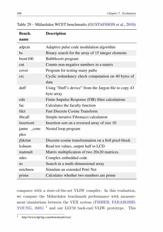
166 Chapter 7. Evaluation
Table 29 – Mälardalen WCET benchmarks (GUSTAFSSON et al., 2010)
Bench.name
Description
adpcm Adaptive pulse code modulation algorithmbs Binary search for the array of 15 integer elementsbsort100 Bubblesort programcnt Counts non-negative numbers in a matrixcover Program for testing many pathscrc Cyclic redundancy check computation on 40 bytes of
dataduff Using “Duff’s device” from the Jargon file to copy 43
byte arrayedn Finite Impulse Response (FIR) filter calculationsfac Calculates the faculty functionfdct Fast Discrete Cosine Transformfibcall Simple iterative Fibonacci calculationinsertsort Insertion sort on a reversed array of size 10janne _com-plex
Nested loop program
jfdctint Discrete-cosine transformation on a 8x8 pixel blocklcdnum Read ten values, output half to LCDmatmult Matrix multiplication of two 20x20 matrices.ndes Complex embedded codens Search in a multi-dimensional arraynsichneu Simulate an extended Petri Netprime Calculates whether two numbers are prime
compares with a state-of-the-art VLIW compiler. In this evaluation,we compare the Mälardalen benchmark performance with measure-ment/simulations between the VEX system (FISHER; FARABOSHI;YOUNG, 2005) 1 and our LLVM back-end/VLIW prototype. This
1 http://www.hpl.hp.com/downloads/vex/
7.1. Impact of the compiler on the performance 167
is the only evaluation we use measurements instead of WCET perfor-mance. Since we do not have access to the framework from other relatedresearches, some of them are proprietary, we use our own framework inorder to estimate worst-case performance enhancement.
7.1 IMPACT OF THE COMPILER ON THE PERFORMANCE
We used the VEX system (FISHER; FARABOSHI; YOUNG,2005) which consists of a VLIW compiler (based on the Multiflow Ccompiler with global trace instruction scheduling) and a parameterizedcycle accurate simulator to demonstrate that different compilers havegreat influence upon performance. VEX is distributed as a binarypackage for the Linux operating system and we do not have access to itssource code. Unfortunately we could not adapt the WCET analyzer forthis platform so this is the only section where the results are evaluatedusing simulation instead of WCET.
We set VEX in a way as similar as possible to the describedarchitecture. Cache configuration is identical (1KB direct mapped).There are the same number of execution units and branch latency isalso identical. The VEX data cache is configured to have null latencyduring miss or write back in order to simulate a scratchpad memoryand its allocation during boot. Some benchmarks are so small thatthis may have a non-null impact on measured performances. We alsoutilized standard compiler optimization flags (-O2) for VEX.
The results of this section regarding the LLVM were obtained byexecuting the compiled and linked benchmarks using the synthesizableVHDL code in ModelSim2 and executing the code on the DE2i-150board. There is a VHDL module who monitors the performance infor-mation. Since there is no variation in the benchmark input data, identi-cal results are obtained executing each benchmark more than once forboth platforms/compilers. In this evaluation, all available hardwarefeatures (predication, branch prediction, etc) are enabled in both VEXand LLVM.
2 Modelsim is a VHDL simulator from Altera’s Quartus Design Suit http://www.altera.com
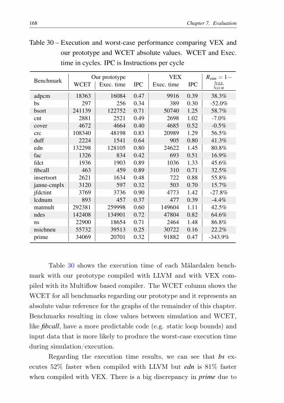
168 Chapter 7. Evaluation
Table 30 – Execution and worst-case performance comparing VEX andour prototype and WCET absolute values. WCET and Exec.time in cycles. IPC is Instructions per cycle
BenchmarkOur prototype VEX Rsim = 1−
WCET Exec. time IPC Exec. time IPC tV EXtLLV M
adpcm 18363 16084 0.47 9916 0.39 38.3%bs 297 256 0.34 389 0.30 -52.0%bsort 241139 122752 0.71 50740 1.25 58.7%cnt 2881 2521 0.49 2698 1.02 -7.0%cover 4672 4664 0.40 4685 0.52 -0.5%crc 108340 48198 0.83 20989 1.29 56.5%duff 2224 1541 0.64 905 0.80 41.3%edn 132298 128105 0.80 24622 1.45 80.8%fac 1326 834 0.42 693 0.51 16.9%fdct 1936 1903 0.89 1036 1.33 45.6%fibcall 463 459 0.89 310 0.71 32.5%insertsort 2621 1634 0.48 722 0.88 55.8%janne-cmplx 3120 597 0.32 503 0.70 15.7%jfdctint 3769 3736 0.90 4773 1.42 -27.8%lcdnum 893 457 0.37 477 0.39 -4.4%matmult 292381 259998 0.60 149604 1.11 42.5%ndes 142408 134901 0.72 47804 0.82 64.6%ns 22900 18654 0.71 2464 1.48 86.8%nsichneu 55732 39513 0.25 30722 0.16 22.2%prime 34069 20701 0.32 91882 0.47 -343.9%
Table 30 shows the execution time of each Mälardalen bench-mark with our prototype compiled with LLVM and with VEX com-piled with its Multiflow based compiler. The WCET column shows theWCET for all benchmarks regarding our prototype and it represents anabsolute value reference for the graphs of the remainder of this chapter.Benchmarks resulting in close values between simulation and WCET,like fibcall, have a more predictable code (e.g. static loop bounds) andinput data that is more likely to produce the worst-case execution timeduring simulation/execution.
Regarding the execution time results, we can see that bs ex-ecutes 52% faster when compiled with LLVM but edn is 81% fasterwhen compiled with VEX. There is a big discrepancy in prime due to
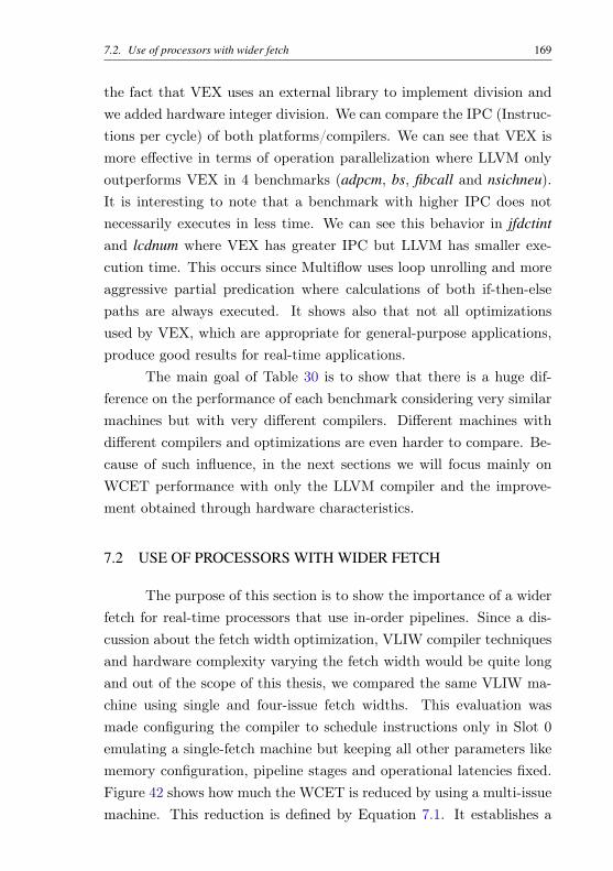
7.2. Use of processors with wider fetch 169
the fact that VEX uses an external library to implement division andwe added hardware integer division. We can compare the IPC (Instruc-tions per cycle) of both platforms/compilers. We can see that VEX ismore effective in terms of operation parallelization where LLVM onlyoutperforms VEX in 4 benchmarks (adpcm, bs, fibcall and nsichneu).It is interesting to note that a benchmark with higher IPC does notnecessarily executes in less time. We can see this behavior in jfdctintand lcdnum where VEX has greater IPC but LLVM has smaller exe-cution time. This occurs since Multiflow uses loop unrolling and moreaggressive partial predication where calculations of both if-then-elsepaths are always executed. It shows also that not all optimizationsused by VEX, which are appropriate for general-purpose applications,produce good results for real-time applications.
The main goal of Table 30 is to show that there is a huge dif-ference on the performance of each benchmark considering very similarmachines but with very different compilers. Different machines withdifferent compilers and optimizations are even harder to compare. Be-cause of such influence, in the next sections we will focus mainly onWCET performance with only the LLVM compiler and the improve-ment obtained through hardware characteristics.
7.2 USE OF PROCESSORS WITH WIDER FETCH
The purpose of this section is to show the importance of a widerfetch for real-time processors that use in-order pipelines. Since a dis-cussion about the fetch width optimization, VLIW compiler techniquesand hardware complexity varying the fetch width would be quite longand out of the scope of this thesis, we compared the same VLIW ma-chine using single and four-issue fetch widths. This evaluation wasmade configuring the compiler to schedule instructions only in Slot 0emulating a single-fetch machine but keeping all other parameters likememory configuration, pipeline stages and operational latencies fixed.Figure 42 shows how much the WCET is reduced by using a multi-issuemachine. This reduction is defined by Equation 7.1. It establishes a
170 Chapter 7. Evaluation
relation between the WCET of each benchmark execution with single-operation and four-operation fetching and it demonstrates how fast thesame program is executed considering worst-case conditions.
R f etch = 1−t f our
tsingle(7.1)
0
5
10
15
20
25
30
35
40
adpc
m bsbs
ort
cnt
cove
rcr
cdu
ffed
nfa
cfd
ctfib
call
inse
rtso
rtja
nne-
cmpl
xjfd
ctin
tlc
dnum
mat
mul
tnd
es nsns
ichn
eupr
ime
%R f
etch
= 1
- tfo
ur/ t
sing
le
Figure 42 – WCET reduction between single-issue and four-issue.
We can see that WCET performance does not depend only on thehardware fetch width but also on the compiler instruction schedulingcapabilities (as discussed earlier in Section 7.1) and on the possibil-ity of parallelization of the code at the instruction level. Because ofthis, we do not observe a WCET reduction of 75% increasing only thefetch width. However, the performance of all benchmarks was increaseddemonstrating the advantage of using VLIW machines in real-time sys-tems. Three of the benchmarks (bs, cnt and cover) decreased theirWCET less than 5%, demonstrating poor instruction parallelization.Others like fdct had 36% of decreased WCET. The fdct – Fast DiscreteCosine Transform – has many calculations based on integer array el-ements and it is highly parallelizable: our LLVM compiler producedan average of 3.20 operations per instruction bundle while bs has only1.23 operations per instruction bundle. With a state-of-the-art com-
7.3. Use of “taken”/“not taken” static branch prediction 171
piler, the performance increase on using a VLIW processor will be evenhigher.
7.3 USE OF “TAKEN”/“NOT TAKEN” STATIC BRANCH PREDIC-TION
Previously we described the branch unit which supports “taken”and “not-taken” static branch predictions. Figure 43 shows how muchthe WCET decreases on using a “taken”/“not taken” solution insteadof only a “not taken” solution. This reduction is defined by Equation7.2 and it relates the WCET between both “taken” and “not-taken”(T-NT) enabled and only “not-taken” (NT) enabled. All other hard-ware features are identically enabled in both WCET computations (twomemory execution units, two multiplication units and predication dis-abled). We have changed only the direction of branches belonging toloops and underlined benchmark labels had null WCET decrease. Theyrequire a compiler WCET oriented static branch prediction as show in(BURGUIERE; ROCHANGE; SAINRAT, 2005) and this is hardwareindependent.
Rbranch = 1− tT−NT
tNT(7.2)
More than half of the benchmarks had WCET reduction whenthe hardware supports both “taken” and “not-taken” predictions. Thereduction depends on the code structure and we can notice that up to12% of reduction could be achieved even without a WCET orientedstatic branch prediction. That demonstrates the importance of branchprediction for high performance real-time systems. It is interesting tonote that the static branch prediction does impact WCET calculationbut could be successfully modeled through different transition flows(Chapter 6).
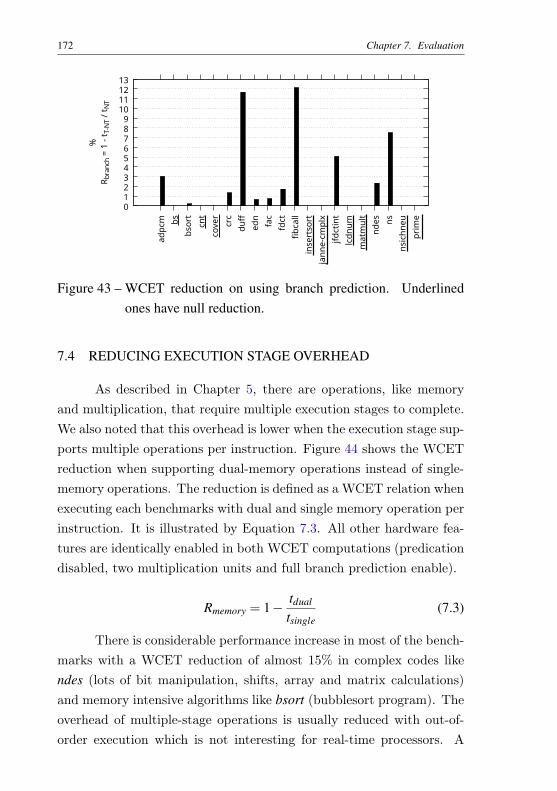
172 Chapter 7. Evaluation
0123456789
10111213
adpc
m bsbs
ort
cnt
cove
rcr
cdu
ffed
nfa
cfd
ctfib
call
inse
rtso
rtja
nne-
cmpl
xjfd
ctin
tlc
dnum
mat
mul
tnd
es nsns
ichn
eupr
ime
%R b
ranc
h=
1 - t
T-N
T/ t
NT
Figure 43 – WCET reduction on using branch prediction. Underlinedones have null reduction.
7.4 REDUCING EXECUTION STAGE OVERHEAD
As described in Chapter 5, there are operations, like memoryand multiplication, that require multiple execution stages to complete.We also noted that this overhead is lower when the execution stage sup-ports multiple operations per instruction. Figure 44 shows the WCETreduction when supporting dual-memory operations instead of single-memory operations. The reduction is defined as a WCET relation whenexecuting each benchmarks with dual and single memory operation perinstruction. It is illustrated by Equation 7.3. All other hardware fea-tures are identically enabled in both WCET computations (predicationdisabled, two multiplication units and full branch prediction enable).
Rmemory = 1− tdual
tsingle(7.3)
There is considerable performance increase in most of the bench-marks with a WCET reduction of almost 15% in complex codes likendes (lots of bit manipulation, shifts, array and matrix calculations)and memory intensive algorithms like bsort (bubblesort program). Theoverhead of multiple-stage operations is usually reduced with out-of-order execution which is not interesting for real-time processors. A
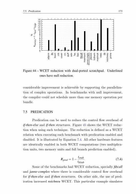
7.5. Predication 173
0123456789
101112131415
adpc
m bsbs
ort
cnt
cove
rcr
cdu
ffed
nfa
cfd
ctfib
call
inse
rtso
rtja
nne-
cmpl
xjfd
ctin
tlc
dnum
mat
mul
tnd
es nsns
ichn
eupr
ime
%R m
emor
y=
1 - t
dual
/ tsi
ngle
Figure 44 – WCET reduction with dual-ported scratchpad. Underlinedones have null reduction.
considerable improvement is achievable by supporting the paralleliza-tion of complex operations. In benchmarks with null improvement,the compiler could not schedule more than one memory operation perbundle.
7.5 PREDICATION
Predication can be used to reduce the control flow overhead ofif-then-else and if-then structures. Figure 45 shows the WCET reduc-tion when using such technique. The reduction is defined as a WCETrelation when executing each benchmark with predication enabled anddisabled. It is illustrated by Equation 7.4. All other hardware featuresare identically enabled in both WCET computations (two multiplica-tion units, two memory units and full branch prediction enabled).
Rpred = 1− tenab
tdisab(7.4)
Some of the benchmarks had WCET reduction, specially fibcalland janne-complex where there is considerable control flow overheadfor if-then-else and if-then structures. On other side, the use of pred-ication increased nsichneu WCET. This particular example simulates
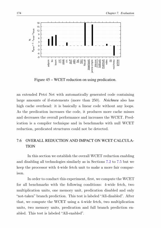
174 Chapter 7. Evaluation
-9
-6
-3
0
3
6
9
12
15
18
adpc
m bsbs
ort
cnt
cove cr
cdu
ffed
nfa
cfd
ctfib
call
inse
rtso
rtja
nne-
cmpl
xjfd
ctin
tlc
dnum
mat
mul
tnd
es nsns
ichn
eupr
ime
%R p
red
= 1
- ten
ab/ t
disa
b
Figure 45 – WCET reduction on using predication.
an extended Petri Net with automatically generated code containinglarge amounts of if-statements (more than 250). Nsichneu also hashigh cache overhead: it is basically a linear code without any loops.As the predication increases the code, it produces more cache missesand decreases the overall performance and increases the WCET. Pred-ication is a compiler technique and in benchmarks with null WCETreduction, predicated structures could not be detected.
7.6 OVERALL REDUCTION AND IMPACT ON WCET CALCULA-TION
In this section we establish the overall WCET reduction enablingand disabling all technologies similarly as in Sections 7.2 to 7.5 but wekeep the processor with 4-wide fetch unit to make a more fair compar-ison.
In order to conduct this experiment, first, we compute the WCETfor all benchmarks with the following conditions: 4-wide fetch, twomultiplication units, one memory unit, predication disabled and only“not-taken” branch prediction. This test is labeled “All-disabled”. Afterthat, we compute the WCET using a 4-wide fetch, two multiplicationunits, two memory units, predication and full branch prediction en-abled. This test is labeled “All-enabled”.
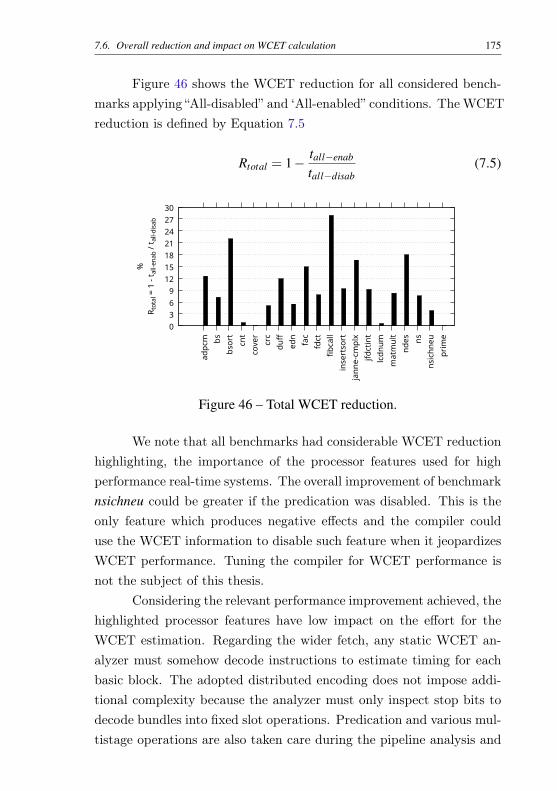
7.6. Overall reduction and impact on WCET calculation 175
Figure 46 shows the WCET reduction for all considered bench-marks applying “All-disabled” and ‘All-enabled” conditions. The WCETreduction is defined by Equation 7.5
Rtotal = 1− tall−enab
tall−disab(7.5)
0369
12151821242730
adpc
m bsbs
ort
cnt
cove
rcr
cdu
ffed
nfa
cfd
ctfib
call
inse
rtso
rtja
nne-
cmpl
xjfd
ctin
tlc
dnum
mat
mul
tnd
es nsns
ichn
eupr
ime
%R t
otal
= 1
- tal
l-ena
b/ t
all-d
isab
Figure 46 – Total WCET reduction.
We note that all benchmarks had considerable WCET reductionhighlighting, the importance of the processor features used for highperformance real-time systems. The overall improvement of benchmarknsichneu could be greater if the predication was disabled. This is theonly feature which produces negative effects and the compiler coulduse the WCET information to disable such feature when it jeopardizesWCET performance. Tuning the compiler for WCET performance isnot the subject of this thesis.
Considering the relevant performance improvement achieved, thehighlighted processor features have low impact on the effort for theWCET estimation. Regarding the wider fetch, any static WCET an-alyzer must somehow decode instructions to estimate timing for eachbasic block. The adopted distributed encoding does not impose addi-tional complexity because the analyzer must only inspect stop bits todecode bundles into fixed slot operations. Predication and various mul-tistage operations are also taken care during the pipeline analysis and
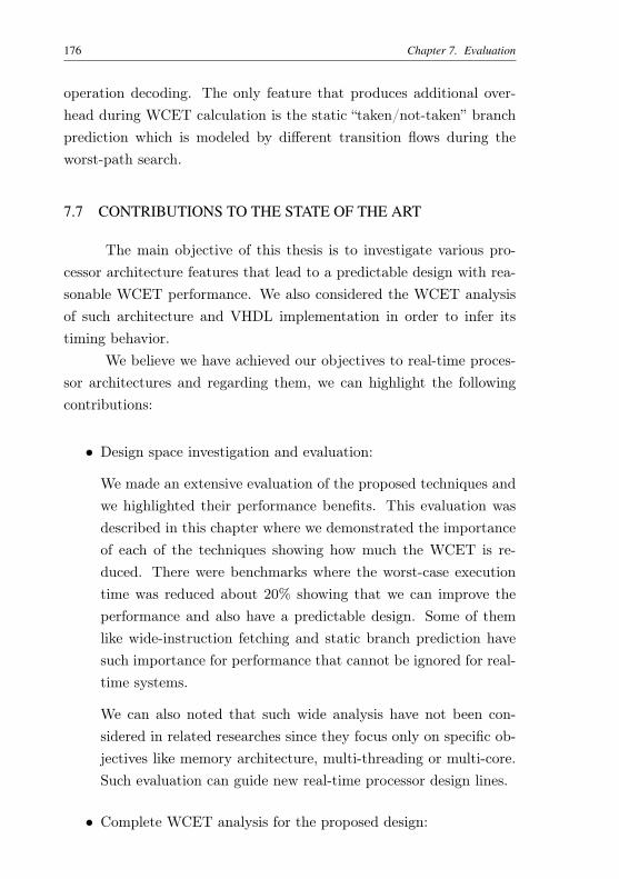
176 Chapter 7. Evaluation
operation decoding. The only feature that produces additional over-head during WCET calculation is the static “taken/not-taken” branchprediction which is modeled by different transition flows during theworst-path search.
7.7 CONTRIBUTIONS TO THE STATE OF THE ART
The main objective of this thesis is to investigate various pro-cessor architecture features that lead to a predictable design with rea-sonable WCET performance. We also considered the WCET analysisof such architecture and VHDL implementation in order to infer itstiming behavior.
We believe we have achieved our objectives to real-time proces-sor architectures and regarding them, we can highlight the followingcontributions:
∙ Design space investigation and evaluation:
We made an extensive evaluation of the proposed techniques andwe highlighted their performance benefits. This evaluation wasdescribed in this chapter where we demonstrated the importanceof each of the techniques showing how much the WCET is re-duced. There were benchmarks where the worst-case executiontime was reduced about 20% showing that we can improve theperformance and also have a predictable design. Some of themlike wide-instruction fetching and static branch prediction havesuch importance for performance that cannot be ignored for real-time systems.
We can also noted that such wide analysis have not been con-sidered in related researches since they focus only on specific ob-jectives like memory architecture, multi-threading or multi-core.Such evaluation can guide new real-time processor design lines.
∙ Complete WCET analysis for the proposed design:
7.7. Contributions to the state of the art 177
We presented all necessary analysis to perform WCET estima-tions of programs compiled for the proposed processor design.Such analyses included cache modeling, pipeline modeling andworst-case path search and they are described in Chapter 6. Theexistence of a WCET analyzer is important in order to achievea predictable hardware design and, an integrated environmentbetween WCET and compiler enhances WCET estimation.
A complete description of a WCET analyzer for a VLIW architec-ture have not been considered in related researches. The Patmosapproach, which is the only one that uses the VLIW approach,uses the commercial aiT3 WCET analyzer. With our WCET an-alyzer and our design space exploration we could identify quan-titatively how much hardware techniques contribute to WCETreduction, as well as how to analyze them during WCET staticestimation.
∙ Complete VHDL design and timing characterization:
We described an implementation of our deterministic real-timeprocessor. We described the timing of each module and theirVHDL implementation which are necessary for WCET modelingand estimation.
Since the related researches focus on specific objectives, a projectlike ours that involves WCET analyzer, compiler and processordesign brings a great research framework for future real-time re-searches.
∙ Detailed branch architecture:
All details of the branch architecture are described including ourmethodology to model it during WCET analyses. We also ex-tended the ISA to support static branch prediction as well as theperformance benefits of using or not this technology in real-timesystems.
3 http://www.absint.com/ait/
178 Chapter 7. Evaluation
Some related researches do not recommend the use of static branchprediction since they add complexity to the WCET analyzer.However, the performance of loop structures are greatly jeop-ardized without branch prediction technology. We showed that apredictable static branch predictor can be analyzed using differ-ent transition flows and it greatly increases performance.
∙ Low overhead full predication system for VLIW processors:
We propose a low-overhead full-predication system without addingoverhead to the hardware data paths or its forwarding logic. Theproposed predication system enhances the support of the singlepath execution as well as loop unrolling techniques. However,predication alone is not enough in order to increase performanceand predictability. The use of predication can actually increasethe WCET. Because of this we propose the use of a hybrid ap-proach with hardware support of a low-overhead predication sys-tem and static branch prediction. This leads to significant WCETreduction and allows compiler WCET optimization by selectingthe appropriate technique.
179
8 FINAL REMARKS
The objective of this thesis was to investigate various processorarchitecture features that lead to a predictable design with reasonableWCET performance. The thesis demonstrated that it is possible toassemble together hardware elements that increase performance butare predictable enough to ensure efficient and precise analyses. Thisis highly motivated by the fact that despite the differences betweengeneral-purpose and embedded computing, the addition of new func-tionality such as audio/video processing, networking, security, automa-tion and control, among others, increases the need for more advancedprocessors for embedded applications. However, deterministic hard-ware is necessary when the application has hard real-time requirements.We can also note that safety standards for embedded applications (DO-178B, DO-178C, IEC-61508, ISO-26262, EN-50125, etc.) require iden-tifying potential functional and non-functional hazards and we mustdemonstrate that the software comply with safety goals. Testing withintensive measurements is tedious and also typically not safe. It is oftenimpossible to prove that the worst-case conditions have actually beentaken into account. As DO-178B succinctly puts it, “testing, in general,cannot show the absence of errors.”
Therefore, it is necessary to analyze the strengths of hardwaretechniques used in state-of-the-art processors, for example temporaland spatial parallelism (pipeline), branch prediction and predication,and to align them to real-time applications. Some of these techniquesrequire modifications due to high hardware complexity while othersneed a well-defined timing behavior. In order to achieve these goals,we propose new approaches in order to improve the efficiency and scal-ability of temporal analysis, especially the worst-case execution timeanalysis. We showed that the design of processors should increase thelevel of importance of the determinism. In this thesis, we focus on do-ing so considering several processor architecture features that lead topredictable design but also improving the WCET performance.
Supporting our objective to investigate and evaluate hardware
180 Chapter 8. Final remarks
features which reconcile determinism and performance, we made thefollowing contributions:
∙ Design space investigation and evaluation regarding VLIW pro-cessors.
∙ Complete WCET analysis for the proposed design.
∙ Complete VHDL design and timing characterization.
∙ Detailed branch architecture.
∙ Low-overhead full-predication system for VLIW processors.
Regarding the design-space investigation and performance eval-uation, we made an intensive investigation of the literature analyzingthe proposed techniques for real-time processors. This investigationlead us to some of our design decisions but there was a lack of perfor-mance evaluations. We knew, for instance, that the use of predicationis interesting for real-time processors but how much this technique con-tributes to WCET performance enhancement and how hard the hard-ware is pushed to support a generic predication system were questionsto be answered. Same doubts turned up on branch prediction as well.Some works propose to not use branch prediction at all but how muchthis hurts pipeline performance? In order to answer these questions,we made an extensive evaluation including the impact of the compileron the performance which is specially important for processors withwide-fetch, in-order execution and static instruction scheduler. Otherexperiments were made to evaluate our design decisions consideringwider fetch, the use or not of branch prediction and predication andthe benefits of dual-port memory access. Most of them lead to signifi-cant WCET reduction while others need more compiler support to befully explored.
It is very important to have a WCET analyzer to infer proprietiesand make performance evaluations. In the context of this work, we usedstate-of-the-art techniques, like the Implicit Path Enumeration Tech-nique (IPET) for worst-case path search, and proposed new strategies
181
in order to estimate WCET of programs running on our VLIW plat-form. Execution of various paths while using predication was modeledduring pipeline analysis as well as the timing of multi-cycle operations.Control-flow instruction timing was also modeled in conjunction withIPET by using different transition flows (δ ) for each type of basic blocktransition. Cache memory behavior was also considered by the WCETanalyzer and, even being a single direct-mapped cache, the modelingof its timing was very challenging specially during validation due tocomplex control-flow structures such as nested loops. We can also notethat an integrated data flow between the compiler and the analyzerillustrated by our tool is very important when implementing a WCETanalyzer. Much of the data required for WCET estimation is alwaysproduced by the compiler, specially the control-flow graph and loop an-notations, and an integration of these tools makes WCET computationmore efficient and precise. With our WCET analyzer and our designspace exploration we could identify quantitatively how much hardwaretechniques contribute to WCET reduction as well as how to analyzethem during WCET static estimation. We concluded that the knowl-edge of a WCET analyzer is important in order to achieve a predictablehardware design and that an integrated environment between WCETand compiler enhances WCET estimation.
We made also a complete VHDL implementation of the proposeddesign. This step was important to infer the timing behavior and thehardware complexity of each module. The use of a hardware descriptionlanguage to implement the design was very challenging. In order toreach the desired clock speed and to use the proper hardware designmethodology, most of the modules were implemented synchronously.Some of them are naturally implemented this way, but the pipelinefront-end required considerable levels of logic with various states inits finite state machine. Large components, like the arithmetic unitsand its forwarding logic have to be optimized in the VHDL code leveland they were pinned to specific FPGA regions in order to reach thedesired performance. The processor researched in this thesis was a 4-wide fetch VLIW microprocessor with 32-bit RISC operations and it
182 Chapter 8. Final remarks
was synthesized on an Altera Cyclone IV GX (EP4CGX150DF31C7) ina DE2i-150 development board. We targeted and reached a clock speedof 100Mhz and it required a total of 21,220 of 149,760 (14%) FPGAcombination function resources. In terms of FPGA memory utilization,it required a total of 1,188,764 of 6,635,520 (15%) memory bits.
Branch architecture has always generated discussion and researchin computer architectures. We showed that static branch prediction isvery important to increase the WCET performance of real-time sys-tems especially for loops which are very predictable. In special, weproved that the use of static branch predication does not add signifi-cant hardware complexity and its WCET analysis is feasible. We mustonly model different basic block transition flows. Since WCET anal-ysis is feasible and it reduces the WCET for more than half of thebenchmarks when the hardware supports both “taken” and “not-taken”predictions, we cannot ignore the use of branch prediction for real-timesystems. We also noted that the WCET reduction depends on the codestructure and up to 12% of reduction could be achieved even withouta WCET-oriented static branch prediction.
Predication has become important for real-time systems becauseit can improve performance and determinism as well, but it adds morecomplexity to hardware and software. Generic full predication addsconsiderable levels of logic to critical processor data paths, specially ininstruction encoding and forwarding paths. The compiler must also bedesigned to use this technology with if-conversions. In terms of hard-ware, we proposed a low-overhead full-predication mechanism in orderto extend the real-time capabilities of the processor. We fixed the pred-icate register, we used only one operation encoding bit and we addedtwo operation modes assisted by special ISA instruction. With thesefeatures, we added full predication support, including complex nestedstructures using full and partial predication, without adding latencies tocritical processor data paths. The support of predication could reducethe WCET of some benchmarks and for some of them this techniquereduced the WCET by about 15%. However, predication alone is notenough in order to increase performance and predictability. The use of
8.1. Publications 183
predication may increase WCET. Because of this we propose the useof a hybrid approach with hardware support of a low-overhead predi-cation system and static branch prediction. This leads to a significantWCET reduction and allows compiler WCET optimization by selectingthe appropriate technique.
We believe we have achieved our objectives contributing to thestate of the art by providing a clear evaluation of the proposed tech-niques as well as a complete framework for further real time researches.We have also secured our low-level requirements focusing on hard real-time systems but also not forgetting the high-level requirements allow-ing our design to be applicable to modern systems using modern ISAand a modern compiler back-end. The VLIW ST231 ISA operationencoding provided a clear and well defined instruction encoding, ade-quate set of arithmetic instructions, typical memory access instructionwith base plus offset addressing mode and allowed the use of func-tion calling/returning. This enhanced the construction of the compilerback-end as well as the decoding during the WCET analysis.
8.1 PUBLICATIONS
This work generated the following publications in conference pro-ceedings:
1. Starke, R. A., Carminati, A., & de Oliveira, R. S. (2015). In-vestigating a four-issue deterministic VLIW architecture for real-time systems. In 2015 IEEE 13th International Conference onIndustrial Informatics (INDIN) (pp. 215–220). Cambrigde - UK:IEEE. http://doi.org/10.1109/INDIN.2015.7281737
2. Silva, K. P., Starke, R. A., & de Oliveira, R. S. (2015). Value anal-ysis for the determination of memory instruction latency in a WCETtool. In 2015 IEEE 13th International Conference on Indus-trial Informatics (INDIN) (pp. 252–257). IEEE. http://doi.org/10.1109/INDIN.2015.7281743
Publication in journals:
184 Chapter 8. Final remarks
1. Starke, R. A., Carminati, A., & de Oliveira, R. S. Evaluating theDesign of a VLIW Processor for Real-Time Systems. ACM Trans-actions on Embedded Computing Systems. Accepted on Decem-ber 7th, 2015. Publication on Vol. 15, No. 3, Article 46. DOI:http://dx.doi.org/10.1145/2889490.
Submitted for publication:
1. Starke, R. A., Carminati, A., & de Oliveira, R. S. Evaluationof a Low Overhead Predication System for a Deterministic VLIWArchitecture Targeting Real-Time Applications. Microprocessorsand Microsystems. Submitted on October 29th, 2015.
2. Carminati, A., Starke, R. A., & de Oliveira, R. S. On implement-ing a WCET analyzer with data integration for a compositional ar-chitecture. Springer Design Automation for Embedded Systems.Submitted on August 25th, 2015.
3. Carminati, A., Starke, R. A., & de Oliveira, R. S. On the Useof Static Branch Prediction to Reduce the Worst-Case ExecutionTime of Real-Time Applications. Journal of System and Software.Submitted on January 6th, 2016.
8.2 SUGGESTIONS OF FUTURE WORK
We believe there are several directions in which this researchcould be continued.
In terms of hardware, the first research is the support of DMA(Direct Memory Access) operations between memories. This featurewill allow the use of a memory hierarchy but its design must considerdeterministic properties like other processor features. On supportinglarge memories with a memory hierarchy, the compiler and the WCETanalyzer should be modified to include the use and analysis of suchfeatures. The use of other types of memories in the first level couldbe also researched: an instruction scratchpad, a data cache memory orsemantic caches like the Patmos approach.
8.2. Suggestions of future work 185
In order to support a complete real-time application with a real-time operating system, peripherals like timers and a vectored interruptcontroller should also be included in the design. This allows avionics orautomotive applications to be used as case studies inferring proprietiesand helping to increase the performance, efficiency and precision of theframework.
In terms of WCET analyzer, a value analysis could be consideredin order to detect unfeasible paths and loop bounds. This technique willgreatly increase the WCET precision and safety. Cache analysis couldalso be improved with a better first miss detection and the support ofassociative caches with Least Recent Use (LRU) eviction policy. Wecould also investigate new methods in order to consider processor tim-ing properties into scheduling equations (e.g. context-switch overheadand shared data).
Working together with the compiler development, the instruc-tion per cycle (IPC) could also be increased with a global instructionscheduler. This also allows a more efficient multi-stage operation de-pendency resolution not stalling the pipeline for all cycles. Our currentcompiler back-end implementation does not consider any Read-After-Write dependencies between pipeline stages and a more sophisticatedhardware dependency resolution will only increase hardware complex-ity. If multi-stage operations could be re-scheduled and reordered, ahardware mechanism could detect the necessary time to satisfy depen-dencies instead of stalling all cycles every time a multi-stage operationis executed. This can also be implemented splitting multiplication anddivision in two parts like the MIPS architecture: first, calculation isdone and its result is read later (a special instruction reads the resultafter the calculation). If we use this strategy, pipeline stall is not nec-essary but the compiler or the hardware must be modified in order tokeep semantics if a result is requested before it is ready.
We can also increase our performance evaluation consideringaverage-case performance generating random input parameters. SinceWCET analysis tools for all related work are not available, we can com-pare our design with others considering small assembly code snippets.

187
BIBLIOGRAPHY
AHO, A. V. et al. Compilers: Principles, Techniques, and Tools. [S.l.]:Pearson Education, 2011. ISBN 9780133002140. 142
ALT, M. et al. Cache behavior prediction by abstract interpretation. In: StaticAnalysis. [S.l.: s.n.], 1996. p. 52–66. 145
BANAKAR, R. et al. Scratchpad memory: a design alternative forcache on-chip memory in embedded systems. Proceedings of the TenthInternational Symposium on Hardware/Software Codesign. CODES 2002(IEEE Cat. No.02TH8627), Acm, p. 73–78, 2002. 62
BURGUIERE, C.; ROCHANGE, C.; SAINRAT, P. A Case for Static BranchPrediction in Real-Time Systems. In: 11th IEEE International Conference onEmbedded and Real-Time Computing Systems and Applications (RTCSA’05).IEEE, 2005. p. 33–38. ISBN 0-7695-2346-3. Disponível em: <http://ieeexplore.ieee.org/lpdocs/epic03/wrapper.htm?arnumber=1541053>. 14,39, 57, 171
CHOI, Y. et al. The Impact of If-conversion and Branch Prediction onProgram Execution on the Intel&Reg; Itanium&Trade; Processor. In:Proceedings of the 34th Annual ACM/IEEE International Symposiumon Microarchitecture. Washington, DC, USA: IEEE Computer Society,2001. (MICRO 34), p. 182–191. ISBN 0-7695-1369-7. Disponível em:<http://dl.acm.org/citation.cfm?id=563998.564023>. 58
CULLMANN, C. et al. Predictability considerations in the design ofmulti-core embedded systems. Ingenieurs de l’Automobile, v. 807, p. 36–42,2010. 141
DAVIS, R. I.; BURNS, A. A survey of hard real-time scheduling formultiprocessor systems. ACM Computing Surveys, v. 43, n. 4, p. 1–44, out.2011. ISSN 03600300. 33
EDWARDS, S. A.; LEE, E. A. The case for the precision timed (PRET)machine. In: Proceedings of the 44th annual conference on Designautomation - DAC ’07. New York, New York, USA: ACM Press, 2007.p. 264. ISBN 9781595936271. ISSN 0738100X. 32
ENGBLOM, J.; JONSSON, B. Processor pipelines and theirproperties for static WCET analysis. In: Embedded Software.[s.n.], 2002. p. 334–348. ISBN 3-540-44307-X. Disponível em:<http://www.springerlink.com/index/J9C2BLLEWB0LMWC1.pdf>. 153
188 Bibliography
FISHER, J. A.; FARABOSHI, P.; YOUNG, C. Emebedded Computing:A VLIW Approach to Architecture Compilers and Tools. [S.l.]: MorganKaufmann Publishers, 2005. 709 p. ISBN 1558607668. 13, 38, 55, 58, 59,83, 85, 125, 166, 167
FISHER, J. A.; MEMBER, S. Trace Scheduling: A Technique forGlobal Microcode Compaction. IEEE Transactions on Computers, C-30,n. 7, p. 478–490, jul. 1981. ISSN 0018-9340. Disponível em: <http://ieeexplore.ieee.org/lpdocs/epic03/wrapper.htm?arnumber=1675827>. 106
GEYER, C. B. et al. Time-predictable code execution - Instruction-setsupport for the single-path approach. In: 16th IEEE International Symposiumon Object/component/service-oriented Real-time distributed Computing(ISORC 2013). IEEE, 2013. p. 1–8. ISBN 978-1-4799-2111-9. Disponívelem: <http://ieeexplore.ieee.org/lpdocs/epic03/wrapper.htm?arnumber=6913195>. 60
GROSSMAN, J. P. Compiler and Architectural Techniques for Improvingthe Effectiveness of VLIW Compilation. [S.l.], 2000. Disponível em:<http://www.ai.mit.edu/projects/aries/>. 59
GRUND, D.; REINEKE, J.; WILHELM, R. A Template for PredictabilityDefinitions with Supporting Evidence. In: LUCAS, P. et al. (Ed.).Bringing Theory to Practice: Predictability and Performance in EmbeddedSystems. Dagstuhl, Germany: Schloss Dagstuhl–Leibniz-Zentrum fuerInformatik, 2011. (OpenAccess Series in Informatics (OASIcs), v. 18),p. 22–31. ISBN 978-3-939897-28-6. ISSN 2190-6807. Disponível em:<http://drops.dagstuhl.de/opus/volltexte/2011/3078>. 35
GUSTAFSSON, J. Usability Aspects of WCET Analysis. 2008 11th IEEEInternational Symposium on Object and Component-Oriented Real-TimeDistributed Computing (ISORC), Ieee, p. 346–352, maio 2008. Disponívelem: <http://ieeexplore.ieee.org/lpdocs/epic03/wrapper.htm?arnumber=4519598>. 12
GUSTAFSSON, J. et al. The M{ä}lardalen WCET Benchmarks - Past,Present and Future. In: Proceedings of the 10th International Workshopon Worst-Case Execution Time Analysis. [s.n.], 2010. Disponível em:<http://www.es.mdh.se/publications/1895->. 22, 40, 82, 165, 166
HWU, W. M. W. et al. The superblock: An effective technique forVLIW and superscalar compilation. The Journal of Supercomputing,v. 7, n. 1-2, p. 229–248, maio 1993. ISSN 0920-8542. Disponívelem: <http://link.springer.com/article/10.1007/BF01205185http://link.springer.com/10.1007/BF01205185>. 105
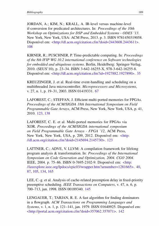
Bibliography 189
JORDAN, A.; KIM, N.; KRALL, A. IR-level versus machine-levelif-conversion for predicated architectures. In: Proceedings of the 10thWorkshop on Optimizations for DSP and Embedded Systems - ODES ’13.New York, New York, USA: ACM Press, 2013. p. 3. ISBN 9781450319058.Disponível em: <http://dl.acm.org/citation.cfm?doid=2443608.2443611>.108
KIRNER, R.; PUSCHNER, P. Time-predictable computing. In: Proceedingsof the 8th IFIP WG 10.2 international conference on Software technologiesfor embedded and ubiquitous systems. Berlin, Heidelberg: Springer-Verlag,2010. (SEUS’10), p. 23–34. ISBN 3-642-16255-X, 978-3-642-16255-8.Disponível em: <http://dl.acm.org/citation.cfm?id=1927882.1927890>. 35
KREUZINGER, J. et al. Real-time event-handling and scheduling on amultithreaded Java microcontroller. Microprocessors and Microsystems,v. 27, n. 1, p. 19–31, 2003. ISSN 01419331. 67
LAFOREST, C.; STEFFAN, J. Efficient multi-ported memories for FPGAs.Proceedings of the ACM/SIGDA 18th International Symposium on FieldProgrammable Gate Arrays, ACM Press, New York, New York, USA, p. 41,2010. 123, 138
LAFOREST, C. E. et al. Multi-ported memories for FPGAs viaXOR. Proceedings of the ACM/SIGDA international symposiumon Field Programmable Gate Arrays - FPGA ’12, ACM Press,New York, New York, USA, p. 209, 2012. Disponível em: <http://dl.acm.org/citation.cfm?doid=2145694.2145730>. 123
LATTNER, C.; ADVE, V. LLVM: A compilation framework for lifelongprogram analysis & transformation. In: Proceedings of the InternationalSymposium on Code Generation and Optimization, 2004. CGO 2004.IEEE, 2004. p. 75–86. ISBN 0-7695-2102-9. Disponível em: <http://ieeexplore.ieee.org/lpdocs/epic03/wrapper.htm?arnumber=1281665>. 40,87, 105, 134, 165
LEE, C.-g. et al. Analysis of cache-related preemption delay in fixed-prioritypreemptive scheduling. IEEE Transactions on Computers, v. 47, n. 6, p.700–713, jun. 1998. ISSN 00189340. 145
LENGAUER, T.; TARJAN, R. E. A fast algorithm for finding dominatorsin a flowgraph. ACM Transactions on Programming Languages andSystems, v. 1, n. 1, p. 121–141, jan. 1979. ISSN 01640925. Disponível em:<http://portal.acm.org/citation.cfm?doid=357062.357071>. 142
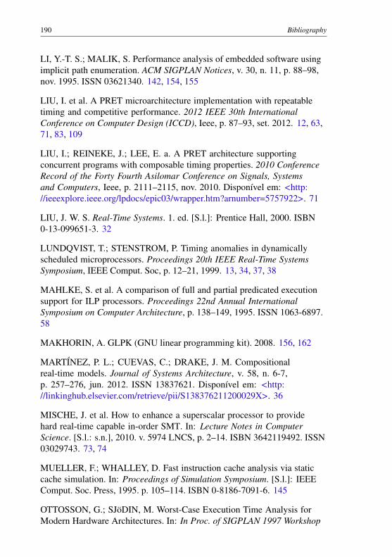
190 Bibliography
LI, Y.-T. S.; MALIK, S. Performance analysis of embedded software usingimplicit path enumeration. ACM SIGPLAN Notices, v. 30, n. 11, p. 88–98,nov. 1995. ISSN 03621340. 142, 154, 155
LIU, I. et al. A PRET microarchitecture implementation with repeatabletiming and competitive performance. 2012 IEEE 30th InternationalConference on Computer Design (ICCD), Ieee, p. 87–93, set. 2012. 12, 63,71, 83, 109
LIU, I.; REINEKE, J.; LEE, E. a. A PRET architecture supportingconcurrent programs with composable timing properties. 2010 ConferenceRecord of the Forty Fourth Asilomar Conference on Signals, Systemsand Computers, Ieee, p. 2111–2115, nov. 2010. Disponível em: <http://ieeexplore.ieee.org/lpdocs/epic03/wrapper.htm?arnumber=5757922>. 71
LIU, J. W. S. Real-Time Systems. 1. ed. [S.l.]: Prentice Hall, 2000. ISBN0-13-099651-3. 32
LUNDQVIST, T.; STENSTROM, P. Timing anomalies in dynamicallyscheduled microprocessors. Proceedings 20th IEEE Real-Time SystemsSymposium, IEEE Comput. Soc, p. 12–21, 1999. 13, 34, 37, 38
MAHLKE, S. et al. A comparison of full and partial predicated executionsupport for ILP processors. Proceedings 22nd Annual InternationalSymposium on Computer Architecture, p. 138–149, 1995. ISSN 1063-6897.58
MAKHORIN, A. GLPK (GNU linear programming kit). 2008. 156, 162
MARTÍNEZ, P. L.; CUEVAS, C.; DRAKE, J. M. Compositionalreal-time models. Journal of Systems Architecture, v. 58, n. 6-7,p. 257–276, jun. 2012. ISSN 13837621. Disponível em: <http://linkinghub.elsevier.com/retrieve/pii/S138376211200029X>. 36
MISCHE, J. et al. How to enhance a superscalar processor to providehard real-time capable in-order SMT. In: Lecture Notes in ComputerScience. [S.l.: s.n.], 2010. v. 5974 LNCS, p. 2–14. ISBN 3642119492. ISSN03029743. 73, 74
MUELLER, F.; WHALLEY, D. Fast instruction cache analysis via staticcache simulation. In: Proceedings of Simulation Symposium. [S.l.]: IEEEComput. Soc. Press, 1995. p. 105–114. ISBN 0-8186-7091-6. 145
OTTOSSON, G.; SJöDIN, M. Worst-Case Execution Time Analysis forModern Hardware Architectures. In: In Proc. of SIGPLAN 1997 Workshop
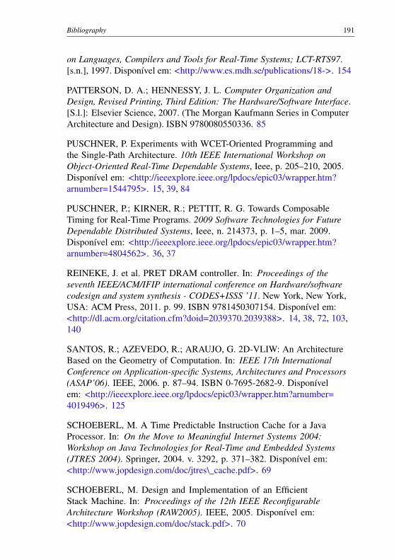
Bibliography 191
on Languages, Compilers and Tools for Real-Time Systems; LCT-RTS97.[s.n.], 1997. Disponível em: <http://www.es.mdh.se/publications/18->. 154
PATTERSON, D. A.; HENNESSY, J. L. Computer Organization andDesign, Revised Printing, Third Edition: The Hardware/Software Interface.[S.l.]: Elsevier Science, 2007. (The Morgan Kaufmann Series in ComputerArchitecture and Design). ISBN 9780080550336. 85
PUSCHNER, P. Experiments with WCET-Oriented Programming andthe Single-Path Architecture. 10th IEEE International Workshop onObject-Oriented Real-Time Dependable Systems, Ieee, p. 205–210, 2005.Disponível em: <http://ieeexplore.ieee.org/lpdocs/epic03/wrapper.htm?arnumber=1544795>. 15, 39, 84
PUSCHNER, P.; KIRNER, R.; PETTIT, R. G. Towards ComposableTiming for Real-Time Programs. 2009 Software Technologies for FutureDependable Distributed Systems, Ieee, n. 214373, p. 1–5, mar. 2009.Disponível em: <http://ieeexplore.ieee.org/lpdocs/epic03/wrapper.htm?arnumber=4804562>. 36, 37
REINEKE, J. et al. PRET DRAM controller. In: Proceedings of theseventh IEEE/ACM/IFIP international conference on Hardware/softwarecodesign and system synthesis - CODES+ISSS ’11. New York, New York,USA: ACM Press, 2011. p. 99. ISBN 9781450307154. Disponível em:<http://dl.acm.org/citation.cfm?doid=2039370.2039388>. 14, 38, 72, 103,140
SANTOS, R.; AZEVEDO, R.; ARAUJO, G. 2D-VLIW: An ArchitectureBased on the Geometry of Computation. In: IEEE 17th InternationalConference on Application-specific Systems, Architectures and Processors(ASAP’06). IEEE, 2006. p. 87–94. ISBN 0-7695-2682-9. Disponívelem: <http://ieeexplore.ieee.org/lpdocs/epic03/wrapper.htm?arnumber=4019496>. 125
SCHOEBERL, M. A Time Predictable Instruction Cache for a JavaProcessor. In: On the Move to Meaningful Internet Systems 2004:Workshop on Java Technologies for Real-Time and Embedded Systems(JTRES 2004). Springer, 2004. v. 3292, p. 371–382. Disponível em:<http://www.jopdesign.com/doc/jtres\_cache.pdf>. 69
SCHOEBERL, M. Design and Implementation of an EfficientStack Machine. In: Proceedings of the 12th IEEE ReconfigurableArchitecture Workshop (RAW2005). IEEE, 2005. Disponível em:<http://www.jopdesign.com/doc/stack.pdf>. 70
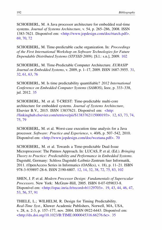
192 Bibliography
SCHOEBERL, M. A Java processor architecture for embedded real-timesystems. Journal of Systems Architecture, v. 54, p. 265–286, 2008. ISSN1383-7621. Disponível em: <http://www.jopdesign.com/doc/rtarch.pdf>.69, 70, 72
SCHOEBERL, M. Time-predictable cache organization. In: Proceedingsof the First International Workshop on Software Technologies for FutureDependable Distributed Systems (STFSSD 2009). [S.l.: s.n.], 2009. 102
SCHOEBERL, M. Time-Predictable Computer Architecture. EURASIPJournal on Embedded Systems, v. 2009, p. 1–17, 2009. ISSN 1687-3955. 31,32, 61, 63, 76
SCHOEBERL, M. Is time predictability quantifiable? 2012 InternationalConference on Embedded Computer Systems (SAMOS), Ieee, p. 333–338,jul. 2012. 35
SCHOEBERL, M. et al. T-CREST: Time-predictable multi-corearchitecture for embedded systems. Journal of Systems Architecture,Elsevier B.V., 2015. ISSN 13837621. Disponível em: <http://linkinghub.elsevier.com/retrieve/pii/S1383762115000193>. 12, 63, 73, 74,75, 79
SCHOEBERL, M. et al. Worst-case execution time analysis for a Javaprocessor. Software: Practice and Experience, v. 40/6, p. 507–542, 2010.Disponível em: <http://www.jopdesign.com/doc/wcetana.pdf>. 70
SCHOEBERL, M. et al. Towards a Time-predictable Dual-IssueMicroprocessor: The Patmos Approach. In: LUCAS, P. et al. (Ed.). BringingTheory to Practice: Predictability and Performance in Embedded Systems.Dagstuhl, Germany: Schloss Dagstuhl–Leibniz-Zentrum fuer Informatik,2011. (OpenAccess Series in Informatics (OASIcs), v. 18), p. 11–21. ISBN978-3-939897-28-6. ISSN 2190-6807. 12, 14, 32, 38, 72, 75, 83, 102
SHEN, J. P. et al. Modern Processor Design: Fundamentals of SuperscalarProcessors. New York: McGraw-Hill, 2005. ISBN 0-07-059033-8.Disponível em: <http://opac.inria.fr/record=b1129703>. 19, 43, 44, 46, 47,53, 56, 57, 91
THIELE, L.; WILHELM, R. Design for Timing Predictability.Real-Time Syst., Kluwer Academic Publishers, Norwell, MA, USA,v. 28, n. 2-3, p. 157–177, nov. 2004. ISSN 0922-6443. Disponível em:<http://dx.doi.org/10.1023/B:TIME.0000045316.66276.6e>. 35
Bibliography 193
UHRIG, S.; MISCHE, J.; UNGERER, T. An IP Core for EmbeddedJava Systems. In: Embedded Computer Systems: Architectures,Modeling, and Simulation. [s.n.], 2007. p. 263–272. Disponível em:<http://link.springer.com/10.1007/978-3-540-73625-7\_28>. 67, 68, 73
UHRIG, S.; WIESE, J. jamuth: an IP processor core for embeddedJava real-time systems. In: Proceedings of the 5th internationalworkshop on Java technologies for real-time and embedded systems -JTRES ’07. [s.n.], 2007. p. 230. ISBN 9781595938138. Disponível em:<http://dl.acm.org/citation.cfm?doid=1288940.1288974>. 68, 69
UNGERER, T. et al. Merasa: Multicore Execution of Hard Real-TimeApplications Supporting Analyzability. IEEE Micro, v. 30, n. 5, p. 66–75,set. 2010. ISSN 0272-1732. 74, 75
WENZEL, I. et al. Principles of Timing Anomalies in SuperscalarProcessors. In: Fifth International Conference on Quality Software. [S.l.]:IEEE, 2005. p. 295–306. ISBN 0-7695-2472-9. 33, 34
WHITHAM, J.; AUDSLEY, N. MCGREP–A Predictable Architecture forEmbedded Real-Time Systems. 2006 27th IEEE International Real-TimeSystems Symposium (RTSS’06), Ieee, p. 13–24, 2006. 70, 71
WHITHAM, J.; AUDSLEY, N. Investigating Average versus Worst-CaseTiming Behavior of Data Caches and Data Scratchpads. 2010 22ndEuromicro Conference on Real-Time Systems, Ieee, p. 165–174, jul. 2010. 62
WHITHAM, J. et al. Investigation of Scratchpad Memory for PreemptiveMultitasking. 2012 IEEE 33rd Real-Time Systems Symposium, Ieee, p. 3–13,dez. 2012. 62
WILHELM, R. et al. The worst-case execution-time problem - overview ofmethods and survey of tools. ACM Transactions on Embedded ComputingSystems, v. 7, n. 3, p. 1–53, abr. 2008. ISSN 15399087. 31, 32


Appendix

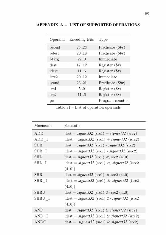
197
APPENDIX A – LIST OF SUPPORTED OPERATIONS
Operand Encoding Bits Type
bcond 25..23 Predicate ($br)bdest 20..18 Predicate ($br)btarg 22..0 Immediatedest 17..12 Register ($r)idest 11..6 Register ($r)isrc2 20..12 Immediatescond 23..21 Predicate ($br)src1 5..0 Register ($r)src2 11..6 Register ($r)pc Program counter
Table 31 – List of operation operands
Mnemonic Semantic
ADD dest = signext32 (src1) + signext32 (src2)ADD_I idest = signext32 (src1) + signext32 (isrc2)SUB dest = signext32 (src1) - signext32 (src2)SUB_I idest = signext32 (src1) - signext32 (isrc2)SHL dest = signext32 (src1) ≪ src2 (4..0)SHL_I idest = signext32 (src1) ≪ signext32 (isrc2
(4..0))SHR dest = signext32 (src1) ≫ src2 (4..0)SHR_I idest = signext32 (src1) ≫ signext32 (isrc2
(4..0))SHRU dest = signext32 (src1) ≫ src2 (4..0)SHRU_I idest = signext32 (src1) ≫ signext32 (isrc2
(4..0))AND dest = signext32 (src1) & signext32 (src2)AND_I idest = signext32 (src1) & signext32 (isrc2)ANDC dest = signext32 (src1) & signext32 (src2)
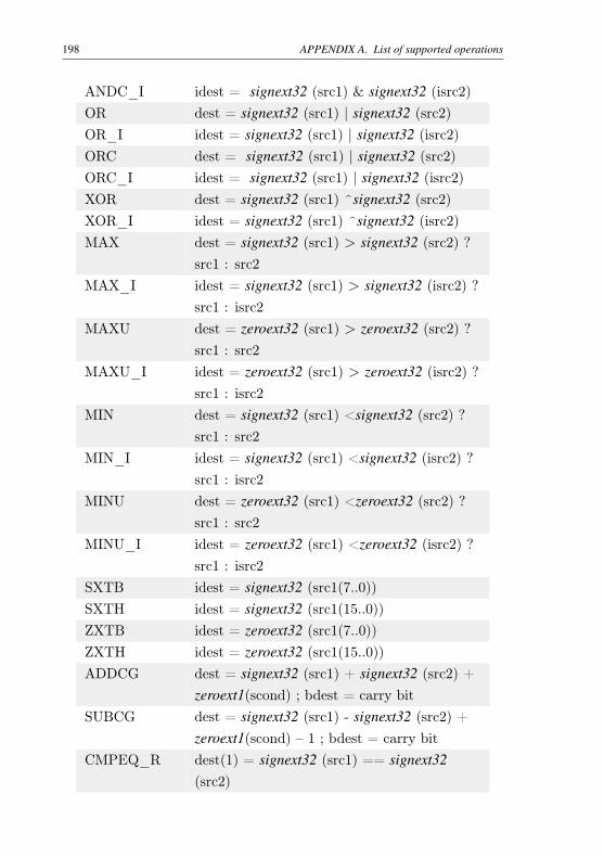
198 APPENDIX A. List of supported operations
ANDC_I idest = signext32 (src1) & signext32 (isrc2)OR dest = signext32 (src1) | signext32 (src2)OR_I idest = signext32 (src1) | signext32 (isrc2)ORC dest = signext32 (src1) | signext32 (src2)ORC_I idest = signext32 (src1) | signext32 (isrc2)XOR dest = signext32 (src1) ^signext32 (src2)XOR_I idest = signext32 (src1) ^signext32 (isrc2)MAX dest = signext32 (src1) > signext32 (src2) ?
src1 : src2MAX_I idest = signext32 (src1) > signext32 (isrc2) ?
src1 : isrc2MAXU dest = zeroext32 (src1) > zeroext32 (src2) ?
src1 : src2MAXU_I idest = zeroext32 (src1) > zeroext32 (isrc2) ?
src1 : isrc2MIN dest = signext32 (src1) <signext32 (src2) ?
src1 : src2MIN_I idest = signext32 (src1) <signext32 (isrc2) ?
src1 : isrc2MINU dest = zeroext32 (src1) <zeroext32 (src2) ?
src1 : src2MINU_I idest = zeroext32 (src1) <zeroext32 (isrc2) ?
src1 : isrc2SXTB idest = signext32 (src1(7..0))SXTH idest = signext32 (src1(15..0))ZXTB idest = zeroext32 (src1(7..0))ZXTH idest = zeroext32 (src1(15..0))ADDCG dest = signext32 (src1) + signext32 (src2) +
zeroext1(scond) ; bdest = carry bitSUBCG dest = signext32 (src1) - signext32 (src2) +
zeroext1(scond) – 1 ; bdest = carry bitCMPEQ_R dest(1) = signext32 (src1) == signext32
(src2)
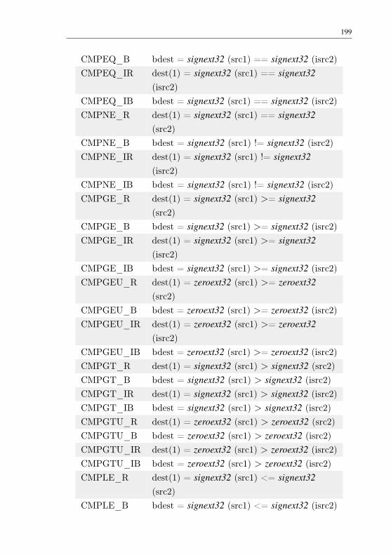
199
CMPEQ_B bdest = signext32 (src1) == signext32 (isrc2)CMPEQ_IR dest(1) = signext32 (src1) == signext32
(isrc2)CMPEQ_IB bdest = signext32 (src1) == signext32 (isrc2)CMPNE_R dest(1) = signext32 (src1) == signext32
(src2)CMPNE_B bdest = signext32 (src1) != signext32 (isrc2)CMPNE_IR dest(1) = signext32 (src1) != signext32
(isrc2)CMPNE_IB bdest = signext32 (src1) != signext32 (isrc2)CMPGE_R dest(1) = signext32 (src1) >= signext32
(src2)CMPGE_B bdest = signext32 (src1) >= signext32 (isrc2)CMPGE_IR dest(1) = signext32 (src1) >= signext32
(isrc2)CMPGE_IB bdest = signext32 (src1) >= signext32 (isrc2)CMPGEU_R dest(1) = zeroext32 (src1) >= zeroext32
(src2)CMPGEU_B bdest = zeroext32 (src1) >= zeroext32 (isrc2)CMPGEU_IR dest(1) = zeroext32 (src1) >= zeroext32
(isrc2)CMPGEU_IB bdest = zeroext32 (src1) >= zeroext32 (isrc2)CMPGT_R dest(1) = signext32 (src1) > signext32 (src2)CMPGT_B bdest = signext32 (src1) > signext32 (isrc2)CMPGT_IR dest(1) = signext32 (src1) > signext32 (isrc2)CMPGT_IB bdest = signext32 (src1) > signext32 (isrc2)CMPGTU_R dest(1) = zeroext32 (src1) > zeroext32 (src2)CMPGTU_B bdest = zeroext32 (src1) > zeroext32 (isrc2)CMPGTU_IR dest(1) = zeroext32 (src1) > zeroext32 (isrc2)CMPGTU_IB bdest = zeroext32 (src1) > zeroext32 (isrc2)CMPLE_R dest(1) = signext32 (src1) <= signext32
(src2)CMPLE_B bdest = signext32 (src1) <= signext32 (isrc2)
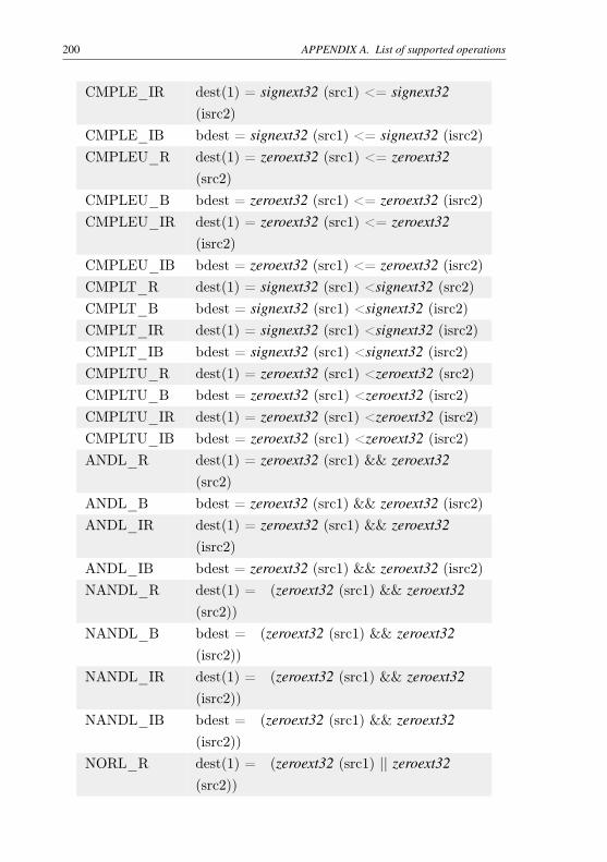
200 APPENDIX A. List of supported operations
CMPLE_IR dest(1) = signext32 (src1) <= signext32(isrc2)
CMPLE_IB bdest = signext32 (src1) <= signext32 (isrc2)CMPLEU_R dest(1) = zeroext32 (src1) <= zeroext32
(src2)CMPLEU_B bdest = zeroext32 (src1) <= zeroext32 (isrc2)CMPLEU_IR dest(1) = zeroext32 (src1) <= zeroext32
(isrc2)CMPLEU_IB bdest = zeroext32 (src1) <= zeroext32 (isrc2)CMPLT_R dest(1) = signext32 (src1) <signext32 (src2)CMPLT_B bdest = signext32 (src1) <signext32 (isrc2)CMPLT_IR dest(1) = signext32 (src1) <signext32 (isrc2)CMPLT_IB bdest = signext32 (src1) <signext32 (isrc2)CMPLTU_R dest(1) = zeroext32 (src1) <zeroext32 (src2)CMPLTU_B bdest = zeroext32 (src1) <zeroext32 (isrc2)CMPLTU_IR dest(1) = zeroext32 (src1) <zeroext32 (isrc2)CMPLTU_IB bdest = zeroext32 (src1) <zeroext32 (isrc2)ANDL_R dest(1) = zeroext32 (src1) && zeroext32
(src2)ANDL_B bdest = zeroext32 (src1) && zeroext32 (isrc2)ANDL_IR dest(1) = zeroext32 (src1) && zeroext32
(isrc2)ANDL_IB bdest = zeroext32 (src1) && zeroext32 (isrc2)NANDL_R dest(1) = (zeroext32 (src1) && zeroext32
(src2))NANDL_B bdest = (zeroext32 (src1) && zeroext32
(isrc2))NANDL_IR dest(1) = (zeroext32 (src1) && zeroext32
(isrc2))NANDL_IB bdest = (zeroext32 (src1) && zeroext32
(isrc2))NORL_R dest(1) = (zeroext32 (src1) || zeroext32
(src2))
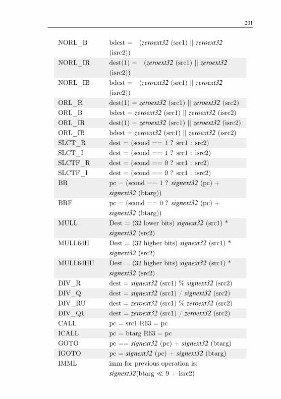
201
NORL_B bdest = (zeroext32 (src1) || zeroext32(isrc2))
NORL_IR dest(1) = (zeroext32 (src1) || zeroext32(isrc2))
NORL_IB bdest = (zeroext32 (src1) || zeroext32(isrc2))
ORL_R dest(1) = zeroext32 (src1) || zeroext32 (src2)ORL_B bdest = zeroext32 (src1) || zeroext32 (isrc2)ORL_IR dest(1) = zeroext32 (src1) || zeroext32 (isrc2)ORL_IB bdest = zeroext32 (src1) || zeroext32 (isrc2)SLCT_R dest = (scond == 1 ? src1 : src2)SLCT_I dest = (scond == 1 ? src1 : isrc2)SLCTF_R dest = (scond == 0 ? src1 : src2)SLCTF_I dest = (scond == 0 ? src1 : isrc2)BR pc = (scond == 1 ? signext32 (pc) +
signext32 (btarg))BRF pc = (scond == 0 ? signext32 (pc) +
signext32 (btarg))MULL Dest = (32 lower bits) signext32 (src1) *
signext32 (src2)MULL64H Dest = (32 higher bits) signext32 (src1) *
signext32 (src2)MULL64HU Dest = (32 higher bits) signext32 (src1) *
signext32 (src2)DIV_R dest = signext32 (src1) % signext32 (src2)DIV_Q dest = signext32 (src1) / signext32 (src2)DIV_RU dest = zeroext32 (src1) % zeroext32 (src2)DIV_QU dest = zeroext32 (src1) / zeroext32 (src2)CALL pc = src1 R63 = pcICALL pc = btarg R63 = pcGOTO pc == signext32 (pc) + signext32 (btarg)IGOTO pc = signext32 (pc) + signext32 (btarg)IMML imm for previous operation is:
signext32(btarg ≪ 9 + isrc2)
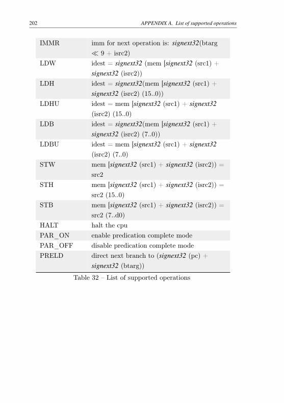
202 APPENDIX A. List of supported operations
IMMR imm for next operation is: signext32(btarg≪ 9 + isrc2)
LDW idest = signext32 (mem [signext32 (src1) +signext32 (isrc2))
LDH idest = signext32(mem [signext32 (src1) +signext32 (isrc2) (15..0))
LDHU idest = mem [signext32 (src1) + signext32(isrc2) (15..0)
LDB idest = signext32(mem [signext32 (src1) +signext32 (isrc2) (7..0))
LDBU idest = mem [signext32 (src1) + signext32(isrc2) (7..0)
STW mem [signext32 (src1) + signext32 (isrc2)) =src2
STH mem [signext32 (src1) + signext32 (isrc2)) =src2 (15..0)
STB mem [signext32 (src1) + signext32 (isrc2)) =src2 (7..d0)
HALT halt the cpuPAR_ON enable predication complete modePAR_OFF disable predication complete modePRELD direct next branch to (signext32 (pc) +
signext32 (btarg))
Table 32 – List of supported operations