Embed Size (px)
Citation preview

REMOVAL OF OIL FROM WATER USING FUNGAL BIOMASS
A Thesis
Submitted to the Faculty of Graduate Studies and Research
In Partial Fulfillment of the Requirements
For the degree of
Doctor of Philosophy
In
Environmental Systems Engineering
University of Regina
By
Asha Srinivasan
Regina, Saskatchewan
February 2012
Copyright 2012: A. Srinivasan

I 1 Library and Archives Canada
Published Heritage Branch
Bibliotheque et Archives Canada
Direction du Patrimoine de ('edition
395 Wellington Street 395, rue Wellington Ottawa ON KlA ON4 Ottawa ON MA ON4 Canada Canada
NOTICE: AVIS:
The author has granted a non-exclusive license allowing Library and Archives Canada to reproduce, publish, archive, preserve, conserve, communicate to the public by telecommunication or on the Internet, loan, distrbute and sell theses worldwide, for commercial or non-commercial purposes, in microform, paper, electronic and/or any other formats.
The author retains copyright ownership and moral rights in this thesis. Neither the thesis nor substantial extracts from it may be printed or otherwise reproduced without the author's permission.
L'auteur a accord permettant a la 131 Canada de repro( sauvegarder, con par telecommunic distribuer et vend monde, a des fine support microforn autres formats.
L'auteur conserve et des droits more la these ni des ex ne doivent etre irr reproduits sans sl
1*1 Library and Archives Bibliotheque et Canada Archives Canada
Published Heritage Direction du Branch Patrimoine de I'edition
395 Wellington Street 395, rue Wellington Ottawa ON K1A 0N4 Ottawa ON K1A 0N4 Canada Canada
NOTICE:
The author has granted a nonexclusive license allowing Library and Archives Canada to reproduce, publish, archive, preserve, conserve, communicate to the public by telecommunication or on the Internet, loan, distrbute and sell theses worldwide, for commercial or noncommercial purposes, in microform, paper, electronic and/or any other formats.
AVIS:
L'auteur a accord permettant a la Bi
Canada de reproc sauvegarder, con partelecommunic distribuer et vend monde, a des fins support microforn autres formats.
The author retains copyright ownership and moral rights in this thesis. Neither the thesis nor substantial extracts from it may be printed or otherwise reproduced without the author's permission.
L'auteur conserve et des droits more la these ni des ex ne doivent etre irr reproduits sans s<

UNIVERSITY OF REGINA
FACULTY OF GRADUATE STUDIES AND RESEARCH
SUPERVISORY AND EXAMINING COMMITTEE
Asha Srinivasan, candidate for the degree of Doctor of Philosophy in Environmental Systems Engineering, has presented a thesis titled, Removal of Oil from Water Using Fungal Biomass, in an oral examination held on December 16, 2011. The following committee members have found the thesis acceptable in form and content, and that the candidate demonstrated satisfactory knowledge of the subject material.
External Examiner:
Co-Supervisor:
Co-Supervisor:
Committee Member:
Committee Member:
Committee Member:
Committee Member:
Chair of Defense:
*Not present at defense
Dr. Jian Peng, University of Saskatchewan
Dr. Tsun Wai Kelvin Ng, Envirnmental Systems Engineering.
Dr. Thiruvenkatachari Viraraghavan, Adjunct
Dr. Yee-Chung Jin, Envirnmental Systems Engineering
Dr. Dena McMartin, Environmental Systems Engineering
Dr. Amr Henni, Industrial Systems Engineering
Dr. Harold Weger, Department of Biology
Dr. Dongyan Blachford, Faculty of Graduate Studies & Research
UNIVERSITY OF REGINA
FACULTY OF GRADUATE STUDIES AND RESEARCH
SUPERVISORY AND EXAMINING COMMITTEE
Asha Srinivasan, candidate for the degree of Doctor of Philosophy in Environmental Systems Engineering, has presented a thesis titled, Removal of Oil from Water Using Fungal Biomass, in an oral examination held on December 16, 2011. The following committee members have found the thesis acceptable in form and content, and that the candidate demonstrated satisfactory knowledge of the subject material.
External Examiner: Dr. Jian Peng, University of Saskatchewan
Co-Supervisor: Dr. Tsun Wai Kelvin Ng, Envirnmental Systems Engineering.
Co-Supervisor: Dr. Thiruvenkatachari Viraraghavan, Adjunct
Committee Member: Dr. Yee-Chung Jin, Envirnmental Systems Engineering
Committee Member: Dr. Dena McMartin, Environmental Systems Engineering
Committee Member: Dr. Amr Henni, Industrial Systems Engineering
Committee Member: Dr. Harold Weger, Department of Biology
Chair of Defense: Dr. Dongyan Blachford, Faculty of Graduate Studies & Research
*Not present at defense

Abstract
The presence of oil in water is of major concern due to its impact on the
environment. Various materials, used to remove oil from water, have either exhibited low
removal efficiencies or are not selective. The use of biomaterials such as bacteria, fungi,
or plant biomass, to adsorb organic substances, has been examined to a limited extent; the
biosorption of oil from water by fungal biomass has not been investigated, so far.
The present study evaluated the potential of non-viable Mucor rouxii biomass
with respect to the removal of three representative oils (Standard Mineral Oil (SMO),
Canola Oil (CO) and Bright-Edge 80 cutting oil) from water via a series of batch and
column adsorption experiments. A preliminary batch adsorption study was conducted to
evaluate oil removal capacities of two non-viable fungal biomasses, Mucor rouxii and
Absidia coerulea. Non- viable M rouxii biomass was found to be more effective than A.
coerulea biomass in removing oil from water. A fractional factorial design analysis was
conducted to screen significant factors influencing the removal of three oils from water
using M rouxii biomass. pH of the solution was observed to be the most influencing
parameter. Temperature had an effect on SMO and Bright-Edge 80 removal while the
adsorbent dose was found to influence the removal of SMO.
Detailed batch adsorption studies were therefore conducted to remove oil from
water using M rouxii biomass by varying the solution pH, the adsorbent dosage, the oil
concentration and the temperature. Adsorption of the three oils on to the M rouxii
biomass followed the pseudo second-order model. On further analysis, adsorption process
was found to have followed the intra-particle diffusion mechanism along with boundary
ii
Abstract
The presence of oil in water is of major concern due to its impact on the
environment. Various materials, used to remove oil from water, have either exhibited low
removal efficiencies or are not selective. The use of biomaterials such as bacteria, fungi,
or plant biomass, to adsorb organic substances, has been examined to a limited extent; the
biosorption of oil from water by fungal biomass has not been investigated, so far.
The present study evaluated the potential of non-viable Mucor rouxii biomass
with respect to the removal of three representative oils (Standard Mineral Oil (SMO),
Canola Oil (CO) and Bright-Edge 80 cutting oil) from water via a series of batch and
column adsorption experiments. A preliminary batch adsorption study was conducted to
evaluate oil removal capacities of two non-viable fungal biomasses, Mucor rouxii and
Absidia coerulea. Non- viable M. rouxii biomass was found to be more effective than A.
coerulea biomass in removing oil from water. A fractional factorial design analysis was
conducted to screen significant factors influencing the removal of three oils from water
using M. rouxii biomass. pH of the solution was observed to be the most influencing
parameter. Temperature had an effect on SMO and Bright-Edge 80 removal while the
adsorbent dose was found to influence the removal of SMO.
Detailed batch adsorption studies were therefore conducted to remove oil from
water using M. rouxii biomass by varying the solution pH, the adsorbent dosage, the oil
concentration and the temperature. Adsorption of the three oils on to the M. rouxii
biomass followed the pseudo second-order model. On further analysis, adsorption process
was found to have followed the intra-particle diffusion mechanism along with boundary
ii

layer diffusion. The Langmuir and Freundlich adsorption models were able to adequately
describe the equilibrium isotherms at different temperatures (5, 15, 22, and 30 °C).
Thermodynamic analysis showed adsorption to be spontaneous and endothermic. The
activation parameters indicated that adsorption was likely diffusion controlled. Chemical
modifications of the biomass and the FTIR analysis showed that carboxyl and amino
groups, present on the M rouxii cell surface were involved in oil sorption.
A continuous column study was carried out using immobilized M rouxii biomass
beads as a biosorbent for the removal of the three oils from water. The Thomas, Yan and
Yoon-Nelson models were found to be suitable in describing column behavior for all
three studied oils. Following column regeneration using de-ionized water, the beads
could be reused to remove oil to that of its initial capacity. Investigations on the
breakdown mechanisms and flow characteristics indicated the possible sequential
occurrence of coalescence and filtration in the immobilized M rouxii biomass bed.
In summary, non-viable M rouxii biomass was found to be an effective medium
for oil removal. This research improves our understanding of the mechanisms
contributing to adsorption of oil by the biomass. Immobilized biomass can be employed
in packed bed columns and re-used to increase their economic attractiveness. The
fundamental understanding of the breakthrough curve behavior is important for process
scale-up under realistic conditions. Further, the study provides a better knowledge on oil-
in-water emulsion flow in coalescing beds. These findings are significant for future
development of filtration systems in coalescing oil droplets that can be used for emulsion
separation.
iii
layer diffusion. The Langmuir and Freundlich adsorption models were able to adequately
describe the equilibrium isotherms at different temperatures (5, 15, 22, and 30 °C).
Thermodynamic analysis showed adsorption to be spontaneous and endothermic. The
activation parameters indicated that adsorption was likely diffusion controlled. Chemical
modifications of the biomass and the FTIR analysis showed that carboxyl and amino
groups, present on the M. rouxii cell surface were involved in oil sorption.
A continuous column study was carried out using immobilized M. rouxii biomass
beads as a biosorbent for the removal of the three oils from water. The Thomas, Yan and
Yoon-Nelson models were found to be suitable in describing column behavior for all
three studied oils. Following column regeneration using de-ionized water, the beads
could be reused to remove oil to that of its initial capacity. Investigations on the
breakdown mechanisms and flow characteristics indicated the possible sequential
occurrence of coalescence and filtration in the immobilized M. rouxii biomass bed.
In summary, non-viable M. rouxii biomass was found to be an effective medium
for oil removal. This research improves our understanding of the mechanisms
contributing to adsorption of oil by the biomass. Immobilized biomass can be employed
in packed bed columns and re-used to increase their economic attractiveness. The
fundamental understanding of the breakthrough curve behavior is important for process
scale-up under realistic conditions. Further, the study provides a better knowledge on oil-
in-water emulsion flow in coalescing beds. These findings are significant for future
development of filtration systems in coalescing oil droplets that can be used for emulsion
separation.
iii

Acknowledgements
I am grateful to my supervisor, Dr. T. Viraraghavan, for his guidance,
encouragement, and understanding that he extended throughout the course of this work. I
thank my co-supervisor, Dr. Kelvin Ng, for his valuable suggestions and assistance in the
preparation of this thesis. I also wish to thank the following members of the dissertation
committee, Dr. Y-C. Jin, Dr. Dena McMartin, Dr. Harold Weger, Dr. Amr Henni and Dr.
Nader Mahinpey for their valuable input over the course of my study.
I would like to acknowledge the assistance of Mr. S. R. Dhanushkodi, University
of Waterloo, who conducted surface area, FTIR and SEM analyses, Dr. Raimar
LObenberg, University of Alberta, who measured the zeta potential of the samples and
Ms. Lauren Bradshaw, University of Regina, who conducted surface area analysis of the
biomaterials. I thank Mr. Herald Berwald who provided the free Bright-Edge 80 cutting
oil used in the study.
I would like to thank the Natural Sciences and Engineering Research Council of
Canada for their financial support to this study by way of a grant to Dr. T. Viraraghavan.
I would like to thank the Faculty of Graduate Studies and Research, University of Regina,
for the partial financial support through graduate scholarships and teaching assistantships.
I also wish to thank the Faculty of Engineering and Applied Science, University of
Regina, for partial financial support.
Above all, I love and appreciate my family for their understanding and moral
support throughout this research.
iv
Acknowledgements
I am grateful to my supervisor, Dr. T. Viraraghavan, for his guidance,
encouragement, and understanding that he extended throughout the course of this work. I
thank my co-supervisor, Dr. Kelvin Ng, for his valuable suggestions and assistance in the
preparation of this thesis. I also wish to thank the following members of the dissertation
committee, Dr. Y-C. Jin, Dr. Dena McMartin, Dr. Harold Weger, Dr. Amr Henni and Dr.
Nader Mahinpey for their valuable input over the course of my study.
I would like to acknowledge the assistance of Mr. S. R. Dhanushkodi, University
of Waterloo, who conducted surface area, FTIR and SEM analyses, Dr. Raimar
Lobenberg, University of Alberta, who measured the zeta potential of the samples and
Ms. Lauren Bradshaw, University of Regina, who conducted surface area analysis of the
biomaterials. I thank Mr. Herald Berwald who provided the free Bright-Edge 80 cutting
oil used in the study.
I would like to thank the Natural Sciences and Engineering Research Council of
Canada for their financial support to this study by way of a grant to Dr. T. Viraraghavan.
I would like to thank the Faculty of Graduate Studies and Research, University of Regina,
for the partial financial support through graduate scholarships and teaching assistantships.
I also wish to thank the Faculty of Engineering and Applied Science, University of
Regina, for partial financial support.
Above all, I love and appreciate my family for their understanding and moral
support throughout this research.
iv
Table of Contents
Abstract ii
Acknowledgements iv
Table of Contents v
List of Figures x
List of Tables xvi
List of Abbreviations, Symbols, Nomenclature xxi
Chapter 1 Introduction 1
1.1 Background 1
1.2 Sources and Quantity of Generated Oily Waters 3
1.3 Existing Treatment Technologies for Oily Water 4
1.4 Environmental Legislation and Concerns 4
1.5 Rationale for using M rouxii Biomass as an Adsorbent for Oil Removal 6
1.6 Objectives and Scope of this Study 8
Chapter 2 Literature Review 11
2.1 Emulsions 11
2.1.1 Classification of Emulsions 11
2.1.2 Physical Characteristics of Emulsions 12
2.1.3 Emulsion Droplet Characteristics 13
2.1.4 Emulsion Stability 14
2.2 Removal of Oil from Water 16
2.2.1 Dissolved Air Flotation 16
v
Table of Contents
Abstract ii
Acknowledgements iv
Table of Contents v
List of Figures x
List of Tables xvi
List of Abbreviations, Symbols, Nomenclature xxi
Chapter 1 Introduction 1
1.1 Background 1
1.2 Sources and Quantity of Generated Oily Waters 3
1.3 Existing Treatment Technologies for Oily Water 4
1.4 Environmental Legislation and Concerns 4
1.5 Rationale for using M. ronxii Biomass as an Adsorbent for Oil Removal 6
1.6 Objectives and Scope of this Study 8
Chapter 2 Literature Review 11
2.1 Emulsions 11
2.1.1 Classification of Emulsions 11
2.1.2 Physical Characteristics of Emulsions 12
2.1.3 Emulsion Droplet Characteristics 13
2.1.4 Emulsion Stability 14
2.2 Removal of Oil from Water 16
2.2.1 Dissolved Air Flotation 16
v

2.2.2 Aerobic Treatment of Oily Wastewater 19
2.2.3 Anaerobic Treatment of Oily Wastewaters 23
2.2.1 Enzymes for the Treatment of Oily Wastewaters 27
2.2.2 Microbial Degradation of Oils 32
2.2.3 Removal of Oil by Various Sorbents 39
2.2.4 Summary 45
2.3 Adsorption Processes in Environmental Engineering 45
2.3.1 Theoretical Background 45
2.3.2 Adsorption Kinetics 46
2.3.3 Adsorption Isotherm 48
2.3.4 Thermodynamic and Activation Parameters 49
2.3.5 Fixed Bed Column in Adsorption Studies 51
2.4 Breakdown Mechanisms 59
2.4.1 Filtration Mechanisms 59
2.4.2 Coalescence Mechanisms 61
Chapter 3 Materials and Methods 66
3.1 Glassware Preparation 66
3.2 Experimental Materials 66
3.3 Preparation of Oil-in-water Emulsions 67
3.4 Characterization of Oil-in-water Emulsions 67
3.5 Preparation of Fungal Seed 68
3.6 Preparation of Non-viable Fungal Biomass 68
vi

3.7 Characterization of Fungal Biomass 69
3.7.1 Surface Area Analysis and Surface Charge Measurement 70
3.7.2 Scanning Electron Microscope (SEM) Studies 70
3.7.3 Fourier Transform Infrared (FTIR) Analysis 71
3.8 Oil Concentration Measurement 71
3.9 Batch Biosorption Experiments 74
3.9.1 Preliminary Studies 75
3.9.2 Factorial Design of Experiments 75
3.9.3 Effect of pH 78
3.9.4 Effect of Concentration 78
3.9.5 Batch Kinetic Studies 79
3.9.6 Batch Isotherm Studies 79
3.9.7 Batch Desorption Studies 80
3.9.8 Modification of Functional Groups and Lipid Extraction 80
3.10 Use of Immobilized Biomass in Oil Removal 82
3.10.1 Procedure for Immobilization of Biomass 82
3.10.2 Characterization of Immobilized M rouxii Beads 82
3.11 Column Studies 83
3.11.1 Continuous Breakthrough Studies 83
3.11.1 Column Regeneration and Reuse 85
3.11.2 Coalescence/ Filtration Experiments 85
Chapter 4 Results and Discussion 89
vii
3.7 Characterization of Fungal Biomass 69
3.7.1 Surface Area Analysis and Surface Charge Measurement 70
3.7.2 Scanning Electron Microscope (SEM) Studies 70
3.7.3 Fourier Transform Infrared (FTIR) Analysis 71
3.8 Oil Concentration Measurement 71
3.9 Batch Biosorption Experiments 74
3.9.1 Preliminary Studies 75
3.9.2 Factorial Design of Experiments 75
3.9.3 Effect of pH 78
3.9.4 Effect of Concentration 78
3.9.5 Batch Kinetic Studies 79
3.9.6 Batch Isotherm Studies 79
3.9.7 Batch Desorption Studies 80
3.9.8 Modification of Functional Groups and Lipid Extraction 80
3.10 Use of Immobilized Biomass in Oil Removal 82
3.10.1 Procedure for Immobilization of Biomass 82
3.10.2 Characterization of Immobilized M. rouxii Be ads 82
3.11 Column Studies 83
3.11.1 Continuous Breakthrough Studies 83
3.11.1 Column Regeneration and Reuse 85
3.11.2 Coalescence/ Filtration Experiments 85
Chapter 4 Results and Discussion 89
vii

4.1 Data and Supplemental Figures 89
4.2 Characterization of Oil 89
4.3 Characterization of M rouxii Biomass and Other Adsorbents 94
4.4 Biosorption of Oil using Different Biomaterials 94
4.5 Factorial Design of Experiments 107
4.5.1 Pareto Plot of Effect 113
4.5.2 Main Effects Plot 113
4.5.3 Interaction Effects Plot 120
4.5.4 Normal Probability Plot of Residuals 124
4.6 Effect of pH on Biosorption 125
4.7 Effect of Concentration on Biosorption 130
4.8 Batch Kinetic Studies 132
4.9 Batch Isotherm Studies 143
4.10 Thermodynamics and Activation Parameters 147
4.11 Batch Desorption Studies 149
4.12 Surface Functional Groups on M rouxii Biomass 149
4.13 Role of Surface Functional Groups, Lipids and Surface Charge on Oil Biosorption
154
4.14 Immobilization of Fungal Biomass and its use in Biosorption 162
4.14.1 Batch Studies using Immobilized Biomass Beads 163
4.15 Column Breakthrough Studies 166
4.15.1 The Thomas Model 166
viii
4.1 Data and Supplemental Figures 89
4.2 Characterization of Oil 89
4.3 Characterization of M. rouxii Z?iomass and Other Adsorbents 94
4.4 Biosorption of Oil using Different Biomaterials 94
4.5 Factorial Design of Experiments 107
4.5.1 Pareto Plot of Effect 113
4.5.2 Main Effects Plot 113
4.5.3 Interaction Effects Plot 120
4.5.4 Normal Probability Plot of Residuals 124
4.6 Effect of pH on Biosorption 125
4.7 Effect of Concentration on Biosorption 130
4.8 Batch Kinetic Studies 132
4.9 Batch Isotherm Studies 143
4.10 Thermodynamics and Activation Parameters 147
4.11 Batch Desorption Studies 149
4.12 Surface Functional Groups on M. rouxii Biomass 149
4.13 Role of Surface Functional Groups, Lipids and Surface Charge on Oil Biosorption
154
4.14 Immobilization of Fungal Biomass and its use in Biosorption 162
4.14.1 Batch Studies using Immobilized Biomass Beads 163
4.15 Column Breakthrough Studies 166
4.15.1 The Thomas Model 166
viii
4.15.2 The Yan Model 171
4.15.3 The Belter and Chu Models 173
4.15.4 The Yoon and Nelson Model 180
4.15.5 The Outman Model 181
4.15.6 The Wolborska Model 181
4.16 Column Regeneration and Reuse 185
4.17 Coalescence/Filtration Mechanism 189
Chapter 5 Conclusion and Recommendations 209
5.1 Conclusion 209
5.2 Practical Research Applications 211
5.3 Contribution to the Field 214
5.4 Recommendations for Further Study 216
References 218
Appendix A Data and Supplementary Figures 248
Appendix B Design of Batch and Column Adsorber System 284
ix
4.15.2 The Yan Model 171
4.15.3 The Belter and Chu Models 173
4.15.4 The Yoon and Nelson Model 180
4.15.5 The Oulman Model 181
4.15.6 The Wolborska Model 181
4.16 Column Regeneration and Reuse 185
4.17 Coalescence/Filtration Mechanism 189
Chapter 5 Conclusion and Recommendations 209
5.1 Conclusion 209
5.2 Practical Research Applications 211
5.3 Contribution to the Field 214
5.4 Recommendations for Further Study 216
References 218
Appendix A Data and Supplementary Figures 248
Appendix B Design of Batch and Column Adsorber System 284
ix

List of Figures
Figure 3.1: Schematics of the experimental set up used for breakthrough studies 84
Figure 3.2: Schematics of the experimental set up used for breakdown studies 86
Figure 4.1: Zeta potential of autoclaved M rouxii biomass and oil-in-water emulsions 91
Figure 4.2: Scanning electron micrographs 96
Figure 4.3: Plot of diameter versus % walnut shell media passing the related sieve 98
Figure 4.4: Adsorption capacity versus time for SMO 99
Figure 4.5: Adsorption capacity versus time for CO 100
Figure 4.6: Adsorption capacity versus time for Bright-Edge 80 101
Figure 4.7: Pareto chart for standardized effects for the removal of SMO 114
Figure 4.8: Pareto chart for standardized effects for the removal of CO 115
Figure 4.9: Pareto chart for standardized effects for the removal of Bright-Edge 80 116
Figure 4.10: Main effects plot for the removal of SMO 117
Figure 4.11: Main effects plot for the removal of CO 118
Figure 4.12: Main effects plot for the removal of Bright-Edge 80 119
Figure 4.13: Interaction effects plot for the removal of SMO 121
Figure 4.14: Interaction effects plot for the removal of CO 122
Figure 4.15: Interaction effects plot for the removal of Bright-Edge 80 123
Figure 4.16: Normal probability plot of the residuals for removal of SMO 126
Figure 4.17: Normal probability plot of the residuals for removal of CO 127
Figure 4.18: Normal probability plot of the residuals for removal of Bright-Edge 80 128
List of Figures
Figure 3.1: Schematics of the experimental set up used for breakthrough studies 84
Figure 3.2: Schematics of the experimental set up used for breakdown studies 86
Figure 4.1: Zeta potential of autoclaved M. rouxii biomass and oil-in-water emulsions 91
Figure 4.2: Scanning electron micrographs 96
Figure 4.3: Plot of diameter versus % walnut shell media passing the related sieve 98
Figure 4.4: Adsorption capacity versus time for SMO 99
Figure 4.5: Adsorption capacity versus time for CO 100
Figure 4.6: Adsorption capacity versus time for Bright-Edge 80 101
Figure 4.7: Pareto chart for standardized effects for the removal of SMO 114
Figure 4.8: Pareto chart for standardized effects for the removal of CO 115
Figure 4.9: Pareto chart for standardized effects for the removal of Bright-Edge 80 116
Figure 4.10: Main effects plot for the removal of SMO 117
Figure 4.11: Main effects plot for the removal of CO 118
Figure 4.12: Main effects plot for the removal of Bright-Edge 80 119
Figure 4.13: Interaction effects plot for the removal of SMO 121
Figure 4.14: Interaction effects plot for the removal of CO 122
Figure 4.15: Interaction effects plot for the removal of Bright-Edge 80 123
Figure 4.16: Normal probability plot of the residuals for removal of SMO 126
Figure 4.17: Normal probability plot of the residuals for removal of CO 127
Figure 4.18: Normal probability plot of the residuals for removal of Bright-Edge 80 128
x

Figure 4.19: Effect of pH on biosorption of oils and zeta potential of autoclaved M rouxii
biomass and three oil-in-water emulsions 129
Figure 4.20: Percentage removal of oil at various initial concentrations 131
Figure 4.21: SMO concentration versus time for different temperatures 133
Figure 4.22: CO concentration versus time for different temperatures 134
Figure 4.23: Bright-Edge 80 concentration versus time for different temperatures 135
Figure 4.24: Rate of SMO biosorption predicted by Lagergren and Ho models at 22°C 140
Figure 4.25: Rate of CO biosorption predicted by Lagergren and Ho models at 22°C 141
Figure 4.26: Rate of Bright-Edge 80 biosorption predicted by Lagergren and Ho models
at 22°C 142
Figure 4.27: Desorption plot for M rouxii biomass using water as an eluent 150
Figure 4.28: FTIR spectra of M rouxii biomass before and after oil adsorption 151
Figure 4.29: FTIR spectra of biomass residue (B1) after methanol and hydrochloric acid
treatment before and after oil adsorption 155
Figure 4.30: FTIR spectra of biomass residue (B2) after formic acid and formaldehyde
treatment before and after oil adsorption 156
Figure 4.31: FTIR spectra of biomass residue (B3) after nitromethane and
triethylphosphite treatment before and after oil adsorption 157
Figure 4.32: FTIR spectra of biomass residue (B4) after acetone treatment before and
after oil adsorption. 158
Figure 4.33: FTIR spectra of biomass residue (B5) after benzene treatment before and
after oil adsorption 159
xi
Figure 4.19: Effect of pH on biosorption of oils and zeta potential of autoclaved M. rouxii
biomass and three oil-in-water emulsions 129
Figure 4.20: Percentage removal of oil at various initial concentrations 131
Figure 4.21: SMO concentration versus time for different temperatures 133
Figure 4.22: CO concentration versus time for different temperatures 134
Figure 4.23: Bright-Edge 80 concentration versus time for different temperatures 135
Figure 4.24: Rate of SMO biosorption predicted by Lagergren and Ho models at 22°C 140
Figure 4.25: Rate of CO biosorption predicted by Lagergren and Ho models at 22°C 141
Figure 4.26: Rate of Bright-Edge 80 biosorption predicted by Lagergren and Ho models
at 22°C 142
Figure 4.27: Desorption plot for M. rouxii biomass using water as an eluent 150
Figure 4.28: FTIR spectra of M. rouxii biomass before and after oil adsorption 151
Figure 4.29: FTIR spectra of biomass residue (Bl) after methanol and hydrochloric acid
treatment before and after oil adsorption 15 5
Figure 4.30: FTIR spectra of biomass residue (B2) after formic acid and formaldehyde
treatment before and after oil adsorption 156
Figure 4.31: FTIR spectra of biomass residue (B3) after nitromethane and
triethylphosphite treatment before and after oil adsorption 157
Figure 4.32: FTIR spectra of biomass residue (B4) after acetone treatment before and
after oil adsorption. 15 8
Figure 4.33: FTIR spectra of biomass residue (B5) after benzene treatment before and
after oil adsorption 15 9
XI
Figure 4.34: Diameter size versus percent of immobilized beads passing the sieve 164
Figure 4.35: Breakthrough curves for SMO predicted using Thomas model 167
Figure 4.36: Breakthrough curves for CO predicted using Thomas model 168
Figure 4.37: Breakthrough curves for Bright-Edge 80 predicted using Thomas model 169
Figure 4.38: Breakthrough curves for SMO predicted using Yan model 174
Figure 4.39: Breakthrough curves for CO predicted using Yan model 175
Figure 4.40: Breakthrough curves for Bright-Edge 80 predicted using Yan model 176
Figure 4.41: Breakthrough curves for SMO predicted using Belter and Chu models 177
Figure 4.42: Breakthrough curves for CO predicted using Belter and Chu models 178
Figure 4.43: Breakthrough curves for Bright-Edge 80 predicted using Belter and Chu
models 179
Figure 4.44: Breakthrough curves for SMO predicted using Yoon and Nelson model 182
Figure 4.45: Breakthrough curves for CO predicted using Yoon and Nelson model 183
Figure 4.46: Breakthrough curves for Bright-Edge 80 using Yoon and Nelson model 184
Figure 4.47: Desorption profile for SMO using de-ionized water 186
Figure 4.48: Desorption profile for CO using de-ionized water 187
Figure 4.49: Desorption profile for Bright-Edge 80 using de-ionized water 188
Figure 4.50: Breakthrough curve for SMO for the second run 190
Figure 4.51: Breakthrough curve for CO for the second run 191
Figure 4.52: Breakthrough curve for Bright-Edge 80 for the second run 192
Figure 4.53: Linearized plot of single-phase flow pressure drop 193
Figure 4.54: Predicted versus actual headloss for single-phase flow 196
xii

Figure 4.55: Linearized plot of two-phase flow pressure drop
Figure 4.56: Predicted versus actual headloss for single-phase flow
Figure 4.57: Coalescence efficiency versus Reynolds number
197
198
202
Figure 4.58: Plot of the ratio of the drop diameter to the immobilized M rouxii biomass
bead diameter versus bed depth for various flow rates 205
Figure 4.59: Average holdup versus Reynolds number 206
Figure 4.60: Coalescence kinetics for SMO predicted by the Crickmore model 208
Figure A.1: Rate of SMO biosorption by Lagergren and Ho kinetic models at 5°C 266
Figure A.2: Rate of SMO biosorption by Lagergren and Ho kinetic models at 15°C 266
Figure A.3: Rate of SMO biosorption by Lagergren and Ho kinetic models at 30°C 267
Figure A.4: Rate of CO biosorption by Lagergren and Ho kinetic models at 5°C 267
Figure A.5: Rate of CO biosorption by Lagergren and Ho kinetic models at 15°C 268
Figure A.6: Rate of CO biosorption by Lagergren and Ho kinetic models at 30°C 268
Figure A.7: Rate of Bright-Edge 80 biosorption by Lagergren and Ho models at 5°C 269
Figure A.8: Rate of Bright-Edge 80 biosorption by Lagergren and Ho models at 15°C 269
Figure A.9: Rate of Bright-Edge 80 biosorption by Lagergren and Ho models at 30°C 270
Figure A.10: Rate of SMO biosorption by intra-particle diffusion model at 5°C 270
Figure A.11: Rate of SMO biosorption by intra-particle diffusion model at 15°C 271
Figure A.12: Rate of SMO biosorption by intra-particle diffusion model at 22°C 271
Figure A.13: Rate of SMO biosorption by intra-particle diffusion model at 30°C 272
Figure A.14: Rate of CO biosorption by intra-particle diffusion model at 5°C 272
Figure A.15: Rate of CO biosorption by intra-particle diffusion model at 15°C 273
Figure 4.55 : Linearized plot of two-phase flow pressure drop 197
Figure 4.56: Predicted versus actual headloss for single-phase flow 198
Figure 4.57: Coalescence efficiency versus Reynolds number 202
Figure 4.58: Plot of the ratio of the drop diameter to the immobilized M. rouxii biomass
bead diameter versus bed depth for various flow rates 205
Figure 4.59: Average holdup versus Reynolds number 206
Figure 4.60: Coalescence kinetics for SMO predicted by the Crickmore model 208
Figure A. 1: Rate of SMO biosorption by Lagergren and Ho kinetic models at 5°C 266
Figure A.2: Rate of SMO biosorption by Lagergren and Ho kinetic models at 15°C 266
Figure A.3: Rate of SMO biosorption by Lagergren and Ho kinetic models at 30°C 267
Figure A.4: Rate of CO biosorption by Lagergren and Ho kinetic models at 5°C 267
Figure A.5: Rate of CO biosorption by Lagergren and Ho kinetic models at 15°C 268
Figure A.6: Rate of CO biosorption by Lagergren and Ho kinetic models at 30°C 268
Figure A.7: Rate of Bright-Edge 80 biosorption by Lagergren and Ho models at 5°C 269
Figure A.8: Rate of Bright-Edge 80 biosorption by Lagergren and Ho models at 15°C 269
Figure A.9: Rate of Bright-Edge 80 biosorption by Lagergren and Ho models at 30°C 270
Figure A. 10: Rate of SMO biosorption by intra-particle diffusion model at 5°C 270
Figure A. 11: Rate of SMO biosorption by intra-particle diffusion model at 15°C 271
Figure A. 12: Rate of SMO biosorption by intra-particle diffusion model at 22°C 271
Figure A. 13: Rate of SMO biosorption by intra-particle diffusion model at 30°C 272
Figure A. 14: Rate of CO biosorption by intra-particle diffusion model at 5°C 272
Figure A. 15: Rate of CO biosorption by intra-particle diffusion model at 15°C 273

Figure A.16: Rate of CO biosorption by infra-particle diffusion model at 22°C 273
Figure A.17: Rate of CO biosorption by intra-particle diffusion model at 30°C 274
Figure A.18: Rate of Bright-Edge 80 biosorption by intra-particle diffusion model at 5°C
274
Figure A.19: Rate of Bright-Edge 80 biosorption by intra-particle diffusion model at
15°C
Figure A.20: Rate of Bright-Edge 80 biosorption by infra-particle diffusion model at
22°C
Figure A.21: Rate of Bright-Edge 80 biosorption by intra-particle diffusion model at
30°C
275
275
276
Figure A.22: The Langmuir and Freundlich isotherm for biosorption of SMO at 5°C 276
Figure A.23: The Langmuir and Freundlich isotherm for biosorption of SMO at 15°C 277
Figure A.24: The Langmuir and Freundlich isotherm for biosorption of SMO at 22°C 277
Figure A.25: The Langmuir and Freundlich isotherm for biosorption of CO at 5°C 278
Figure A.26: The Langmuir and Freundlich isotherm for biosorption of CO at 22°C 278
Figure A.27: The Langmuir and Freundlich isotherm for biosorption of CO at 30°C 279
Figure A.28: The Langmuir and Freundlich isotherm model plots for biosorption of
Bright-Edge 80 at 5°C 279
Figure A.29: The Langmuir and Freundlich isotherm model plots for biosorption of
Bright-Edge 80 at 22 °C 280
Figure A.30: The Langmuir and Freundlich isotherm model plots for biosorption of
Bright-Edge 80 at 30 °C 280
xiv
Figure A. 16: Rate of CO biosorption by intra-particle diffusion model at 22°C 273
Figure A. 17: Rate of CO biosorption by intra-particle diffusion model at 30°C 274
Figure A. 18: Rate of Bright-Edge 80 biosorption by intra-particle diffusion model at 5°C
274
Figure A. 19: Rate of Bright-Edge 80 biosorption by intra-particle diffusion model at
15°C 275
Figure A.20: Rate of Bright-Edge 80 biosorption by intra-particle diffusion model at
22°C 275
Figure A.21: Rate of Bright-Edge 80 biosorption by intra-particle diffusion model at
30°C 276
Figure A.22: The Langmuir and Freundlich isotherm for biosorption of SMO at 5°C 276
Figure A.23: The Langmuir and Freundlich isotherm for biosorption of SMO at 15°C 277
Figure A.24: The Langmuir and Freundlich isotherm for biosorption of SMO at 22°C 277
Figure A.25: The Langmuir and Freundlich isotherm for biosorption of CO at 5°C 278
Figure A.26: The Langmuir and Freundlich isotherm for biosorption of CO at 22°C 278
Figure A.27: The Langmuir and Freundlich isotherm for biosorption of CO at 30°C 279
Figure A.28: The Langmuir and Freundlich isotherm model plots for biosorption of
Bright-Edge 80 at 5°C 279
Figure A.29: The Langmuir and Freundlich isotherm model plots for biosorption of
Bright-Edge 80 at 22 °C 280
Figure A.30: The Langmuir and Freundlich isotherm model plots for biosorption of
Bright-Edge 80 at 30 °C 280
xiv

Figure A.31: Breakthrough curve predicted by Oulman model for SMO 281
Figure A.32: Breakthrough curve predicted by Oulman model for CO 281
Figure A.33: Breakthrough curve predicted by Oulman model for Bright-Edge 80 282
Figure A.34: Breakthrough curve predicted by Wolbroska model for SMO 282
Figure A.35: Breakthrough curve predicted by Wolbroska model for CO 283
Figure A.36: Breakthrough curve predicted by Wolbroska model for Bright-Edge 80 283
xv

List of Tables
Table 1.1: Chitosan content in fungi 7
Table 2.1: Biological treatment 28
Table 2.2: Microbial degradation 40
Table 2.3: Oil sorption capacity of different media 43
Table 2.4: Design criteria for packed bed columns 53
Table 2.5: Design details of lab scale columns used in biosorption studies 54
Table 3.1: Oil in water measurement methods 72
Table 3.2: Coded and uncoded values of the factors 76
Table 4.1: Characteristics of oils used for the study at 20°C 90
Table 4.2: Characteristics of the solvent used in the measurement of oil 92
Table 4.3: Emulsion classification based on the diameter of oil droplets 93
Table 4.4: Characteristics of M rouxii biomass 95
Table 4.5: Characteristics of other adsorbents used in the preliminary study 97
Table 4.6: Residual oil concentration obtained using different biomaterials 102
Table 4.7: Oil removals by biomaterials 104
Table 4.8: Uncoded design table for the factors and response 108
Table 4.9: Estimated effects and coefficients for the removal of SMO (% coded units) 109
Table 4.10: Estimated effects and coefficients for the removal of CO (% coded units) 110
Table 4.11: Estimated effects and coefficients for the removal of Bright-Edge 80 (%
coded units) 111
xvi
List of Tables
Table 1.1: Chitosan content in fungi 7
Table 2.1: Biological treatment 28
Table 2.2: Microbial degradation 40
Table 2.3: Oil sorption capacity of different media 43
Table 2.4: Design criteria for packed bed columns 53
Table 2.5: Design details of lab scale columns used in biosorption studies 54
Table 3.1: Oil in water measurement methods 72
Table 3.2: Coded and uncoded values of the factors 76
Table 4.1: Characteristics of oils used for the study at 20°C 90
Table 4.2: Characteristics of the solvent used in the measurement of oil 92
Table 4.3: Emulsion classification based on the diameter of oil droplets 93
Table 4.4: Characteristics of M. rouxii biomass 95
Table 4.5: Characteristics of other adsorbents used in the preliminary study 97
Table 4.6: Residual oil concentration obtained using different biomaterials 102
Table 4.7: Oil removals by biomaterials 104
Table 4.8: Uncoded design table for the factors and response 108
Table 4.9: Estimated effects and coefficients for the removal of SMO (% coded units) 109
Table 4.10: Estimated effects and coefficients for the removal of CO (% coded units) 110
Table 4.11: Estimated effects and coefficients for the removal of Bright-Edge 80 (%
coded units) 111
xvi

Table 4.12: Comparison of oil removal efficiencies of M rouxii biomass and other
sorbents obtained in batch studies
Table 4.13: Parameters calculated using kinetic models
Table 4.14: Isotherm model constants
Table 4.15: Separation factor, RL based on the Langmuir equation
Table 4.16: Thermodynamic and activation parameter
137
138
145
146
148
Table 4.17: Functional groups of autoclaved biomass of M rouxii biomass, oil adsorbed
biomass and the corresponding infrared absorption wavelengths (Lin-Vien 1991) 152
Table 4.18: Oil removal by raw and chemically modified M rouxii biomass 160
Table 4.19: Characteristics of immobilized M rouxii biomass 165
Table 4.20: Parameters calculated using kinetic models 170
Table 4.21: Comparison of Thomas constants for other oil sorbents 172
Table 4.22: Summary of coalescence and filtration data 195
Table 4.23: Average saturation values of the immobilized M rouxii biomass bed 200
Table 4.24: Coalescence efficiency 201
Table 5.1: Cost of adsorbents required to treat 100 m3 per day of oily water based on
SMO data 212
Table 5.2: Design of batch adsorber system for M rouxii biomass and SMO with a flow
rate of 100 m3 per day 213
Table 5.3: Design of immobilized M rouxii filter for SMO with a flow rate of 100 m3 per
day 215
Table A.1: Batch kinetic data for SMO 248
xvii
Table 4.12: Comparison of oil removal efficiencies of M. rouxii biomass and other
sorbents obtained in batch studies 137
Table 4.13: Parameters calculated using kinetic models 138
Table 4.14: Isotherm model constants 145
Table 4.15: Separation factor, RL based on the Langmuir equation 146
Table 4.16: Thermodynamic and activation parameter 148
Table 4.17: Functional groups of autoclaved biomass of M. rouxii biomass, oil adsorbed
biomass and the corresponding infrared absorption wavelengths (Lin-Vien 1991) 152
Table 4.18: Oil removal by raw and chemically modified M. rouxii biomass 160
Table 4.19: Characteristics of immobilized M. rouxii biomass 165
Table 4.20: Parameters calculated using kinetic models 170
Table 4.21: Comparison of Thomas constants for other oil sorbents 172
Table 4.22: Summary of coalescence and filtration data 195
Table 4.23: Average saturation values of the immobilized M. rouxii biomass bed 200
Table 4.24: Coalescence efficiency 201
Table 5.1: Cost of adsorbents required to treat 100 m3 per day of oily water based on
SMOdata 212
Table 5.2: Design of batch adsorber system for M. rouxii biomass and SMO with a flow
rate of 100 m3 per day 213
Table 5.3: Design of immobilized M rouxii filter for SMO with a flow rate of 100 m3 per
day 215
Table A. 1: Batch kinetic data for SMO 248
xvii

Table A.2: Batch kinetic data for CO 249
Table A.3: Batch kinetic data for Bright-Edge 80 250
Table A.4: Batch isotherm data for SMO 250
Table A.5: Batch isotherm data for CO 251
Table A.6: Batch isotherm data for Bright-Edge 80 251
Table A.7: Desorption data for SMO 251
Table A.8: Desorption data for CO 252
Table A.9: Desorption data for Bright-Edge 80 252
Table A.10: Batch study with immobilized biomass beads for 6 h 253
Table A.11: Batch kinetic studies with immobilized biomass beads at pH 3.0 253
Table A.12: Column breakthrough data 254
Table A.13: Column desorption data for SMO 255
Table A.14: Column desorption data for CO 255
Table A.15: Column desorption data for Bright-Edge 80 256
Table A.16: Column breakthrough second run data for SMO 256
Table A.17: Column breakthrough second run data for CO 257
Table A.18: Column breakthrough second run data for Bright-Edge 80 257
Table A.19: Experimental and predicted head loss for single-phase flow 258
Table A.20: Experimental and predicted head loss for two-phase flow 259
Table A.21: Drop diameters (gm) for 12 mL/min 260
Table A.22: Drop density (no./ cm3) for 12 mL/min 260
Table A.23: Coalescence efficiency for 12 mL/min 261
xviii
Table A.2: Batch kinetic data for CO 249
Table A.3: Batch kinetic data for Bright-Edge 80 250
Table A.4: Batch isotherm data for SMO 250
Table A.5: Batch isotherm data for CO 251
Table A.6: Batch isotherm data for Bright-Edge 80 251
Table A.7: Desorption data for SMO 251
Table A.8: Desorption data for CO 252
Table A.9: Desorption data for Bright-Edge 80 252
Table A. 10: Batch study with immobilized biomass beads for 6 h 253
Table A. 11: Batch kinetic studies with immobilized biomass beads at pH 3.0 253
Table A. 12: Column breakthrough data 254
Table A. 13: Column desorption data for SMO 255
Table A. 14: Column desorption data for CO 255
Table A. 15: Column desorption data for Bright-Edge 80 256
Table A. 16: Column breakthrough second run data for SMO 256
Table A.17: Column breakthrough second run data for CO 257
Table A. 18: Column breakthrough second run data for Bright-Edge 80 257
Table A. 19: Experimental and predicted head loss for single-phase flow 258
Table A.20: Experimental and predicted head loss for two-phase flow 259
Table A.21: Drop diameters (|im) for 12 mL/min 260
Table A.22: Drop density (no./ cm3) for 12 mL/min 260
Table A.23: Coalescence efficiency for 12 mL/min 261
xviii

Table A.24: Drop diameters (gm) for 16 mL/min 261
Table A.25: Drop density (no./ cm3) for 16 mL/min 261
Table A.26: Coalescence efficiency for 16 mL/min 262
Table A.27: Drop diameters (µm) for 20 mL/min 262
Table A.28: Drop density (no./ cm3) for 20 mL/min 262
Table A.29: Coalescence efficiency for 20 mL/min 263
Table A.30: Drop diameters (gm) for 24 mL/min 263
Table A.31: Drop density (no./ cm3) for 24 mL/min 263
Table A.32: Coalescence efficiency for 24 mL/min 264
Table A.33: Drop diameters (µm) for 28 mL/min 264
Table A.34: Drop density (no./ cm3) for 28 mL/min 264
Table A.35: Coalescence efficiency for 28 mL/min 264
Table A.36: Drop diameters (gm) for 32 mL/min 265
Table A.37: Drop density (no./ cm3) for 32 mL/min 265
Table A.38: Coalescence efficiency for 32 mL/min 265
Table A.39: Data used to fit Crickmore model 265
Table Bl: Design of batch adsorber system for M rouxii biomass and SMO with a flow
rate of 100 m3/d 284
Table B2: Design of batch adsorber system for M rouxii biomass and CO with a flow
rate of 100 m3/d 284
Table B3: Design of batch adsorber system for M rouxii biomass and Bright-Edge 80
with a flow rate of 100 m3/d 285
xix
Table A.24: Drop diameters (urn) for 16 mL/min 261
Table A.25: Drop density (no./ cm3) for 16 mL/min 261
Table A.26: Coalescence efficiency for 16 mL/min 262
Table A.27: Drop diameters (|im) for 20 mL/min 262
Table A.28: Drop density (no./ cm3) for 20 mL/min 262
Table A.29: Coalescence efficiency for 20 mL/min 263
Table A.30: Drop diameters (urn) for 24 mL/min 263
Table A.31: Drop density (no./ cm3) for 24 mL/min 263
Table A.32: Coalescence efficiency for 24 mL/min 264
Table A.33: Drop diameters (|im) for 28 mL/min 264
Table A.34: Drop density (no./ cm3) for 28 mL/min 264
Table A.35: Coalescence efficiency for 28 mL/min 264
Table A.36: Drop diameters (jam) for 32 mL/min 265
Table A.37: Drop density (no./ cm3) for 32 mL/min 265
Table A.38: Coalescence efficiency for 32 mL/min 265
Table A.39: Data used to fit Crickmore model 265
Table Bl: Design of batch adsorber system for M. rouxii biomass and SMO with a flow
rate of 100 m3/d 284
Table B2: Design of batch adsorber system for M. rouxii biomass and CO with a flow
rate of 100 m3/d 284
Table B3: Design of batch adsorber system for M. rouxii biomass and Bright-Edge 80
with a flow rate of 100 m3/d 285
xix

Table B4: Design of immobilized M rouxii biomass column filter for SMO with a flow
rate of 100 m3/d 286
Table B5: Design of immobilized M rouxii biomass column filter for CO with a flow rate
of 100 m3/d
Table B6: Design of immobilized M rouxii biomass column filter for Bright-Edge 80
with a flow rate of 100 m3/d
xx
287
288
Table B4: Design of immobilized M. rouxii biomass column filter for SMO with a flow
rate of 100 m3/d 286
Table B5: Design of immobilized M. rouxii biomass column filter for CO with a flow rate
of 100 m3/d 287
Table B6: Design of immobilized M. rouxii biomass column filter for Bright-Edge 80
with a flow rate of 100 m3/d 288
xx
List of Abbreviations, Symbols, Nomenclature
A Arrhenius factor
a Yan constant denoting the slope of the function.
b Langmuir constant
Bo Specific permeability coefficient
BOD Biological oxygen demand
C Concentration of solute in solution at equilibrium
C Effluent concentration
Co Influent concentration
CA Fraction of fluid emulsified
CA0 Fraction of fluid emulsified at entrance to the packed bed
Ce Equilibrium solute concentration
CO Canola oil
COD Chemical oxygen demand
Cs Concentration of solute in solution
d Throughput volume
DAF Dissolved air flotation
df Average diameter of immobilized biomass beads
di Average particle size of the distribution
Ead Activation energy for adsorption
EPA Environmental Protection Agency
erf(x) Error function of x
xxi
List of Abbreviations, Symbols, Nomenclature
A Arrhenius factor
a Yan constant denoting the slope of the function.
b Langmuir constant
Bo Specific permeability coefficient
BOD Biological oxygen demand
C Concentration of solute in solution at equilibrium
C Effluent concentration
Co Influent concentration
CA Fraction of fluid emulsified
CAO Fraction of fluid emulsified at entrance to the packed bed
Ce Equilibrium solute concentration
CO Canola oil
COD Chemical oxygen demand
Cs Concentration of solute in solution
d Throughput volume
DAF Dissolved air flotation
df Average diameter of immobilized biomass beads
dj Average particle size of the distribution
Ead Activation energy for adsorption
EPA Environmental Protection Agency
erf(x) Error function of x
xxi

FTIR Fourier transform infrared analysis
GAC Granular activated carbon
gc Acceleration due to gravity
K Rate constant of adsorption used in Arrhenius equation
K Adsorption rate coefficient
ko Shape factor
ki Lagergren rate constant for adsorption
k1 Carman-Kozeny constant for single-phase flow
k2 Pseudo-second order adsorption rate constant
k2 Carman-Kozeny constant for two-phase flow
kc Crickmore rate constant for coalescence
KF Freundlich equilibrium constant indicative of adsorption capacity
Intra-particle diffusion rate constant
kJ Kilo joule
Kr Thomas rate constant
KyN Yoon Nelson rate constant
L Bed length
m Mass of the adsorbent
n Freundlich adsorption equilibrium constant indicative of adsorption
intensity
N Adsorption capacity coefficient
Na Saturation concentration in the Wolborska model
FTIR Fourier transform infrared analysis
GAC Granular activated carbon
gc Acceleration due to gravity
K Rate constant of adsorption used in Arrhenius equation
K Adsorption rate coefficient
ko Shape factor
k\ Lagergren rate constant for adsorption
ki Carman-Kozeny constant for single-phase flow
ki Pseudo-second order adsorption rate constant
k2 Carman-Kozeny constant for two-phase flow
kc Crickmore rate constant for coalescence
Kp Freundlich equilibrium constant indicative of adsorption capacity
ki Intra-particle diffusion rate constant
kJ Kilo joule
Kj Thomas rate constant
KYN Yoon Nelson rate constant
L Bed length
m Mass of the adsorbent
n Freundlich adsorption equilibrium constant indicative of adsorption
intensity
N Adsorption capacity coefficient
N0 Saturation concentration in the Wolborska model
xxii

NRe Reynolds number
OMW Olive mill wastewater
POME Palm oil mill effluent
q Amount of adsorbate adsorbed per unit mass of adsorbent
Q Volumetric flow rate
Qo Langmuir constant
ge Amount of adsorbate adsorbed at equilibrium
qt Amount of adsorbate adsorbed at time t
R Universal gas constant
RBC Rotating biological contactor
RL Separation factor
Sd Average saturation
SEM Scanning electron microscope
SMO Standard mineral oil
t Residence time inside the column
T Tortuosity
to Temporal parameter
tin Time required for 50% adsorbate breakthrough
Te Absolute temperature
U Superficial velocity
UASB Upflow anaerobic sludge blanket digestion
UASFF Upflow anaerobic sludge-fixed film
Np_e Reynolds number
OMW Olive mill wastewater
POME Palm oil mill effluent
q Amount of adsorbate adsorbed per unit mass of adsorbent
Q Volumetric flow rate
Qo Langmuir constant
qe Amount of adsorbate adsorbed at equilibrium
q, Amount of adsorbate adsorbed at time t
R Universal gas constant
RBC Rotating biological contactor
RL Separation factor
Sa Average saturation
SEM Scanning electron microscope
SMO Standard mineral oil
t Residence time inside the column
T Tortuosity
to Temporal parameter
ti/2 Time required for 50% adsorbate breakthrough
Te Absolute temperature
U Superficial velocity
UASB Upflow anaerobic sludge blanket digestion
UASFF Upflow anaerobic sludge-fixed film
xxiii

V Throughput volume
VFA Volatile fatty acids
VORW Vegetable oil refinery wastewater
X„, Amount of solute adsorbed in forming a complete monolayer
Z Height of the column
AG° Gibbs free energy change
AFP Heat of adsorption or enthalpy change
API Pressure drop across the bed for single-phase flow
AP2 Pressure drop across the bed for two-phase flow
AS° Entropy change
13a Kinetic coefficient of the external mass transfer
Ye Dynamic viscosity of continuous phase
E Porosity of immobilized biomass bed in single-phase flow
Et Porosity of immobilized biomass bed in two-phase flow
ric Overall coalescence efficiency
a Standard deviation
t Residence time
'E' Modified residence time
(I)H Average holdup
xxiv
V Throughput volume
VFA Volatile fatty acids
VORW Vegetable oil refinery wastewater
Xm Amount of solute adsorbed in forming a complete monolayer
Z Height of the column
AG0 Gibbs free energy change
A/f° Heat of adsorption or enthalpy change
APi Pressure drop across the bed for single-phase flow
AP2 Pressure drop across the bed for two-phase flow
AS0 Entropy change
Pa Kinetic coefficient of the external mass transfer
yc Dynamic viscosity of continuous phase
e Porosity of immobilized biomass bed in single-phase flow
et Porosity of immobilized biomass bed in two-phase flow
r|c Overall coalescence efficiency
a Standard deviation
x Residence time
x' Modified residence time
4>H Average holdup
xxiv

Chapter 1
Introduction
1.1 Background
Rapid urbanization creates an annual increase in the discharge of oil-containing
wastewater into the environment. Oil and grease in wastewater constitute a complex,
heterogeneous matrix and their sources range from the hydrocarbons (petroleum based)
to fatty matter from animal and vegetable sources (Franson and Eaton 2005). Oils can
cause environmental pollution during various stages of production, transportation,
refining and utilization. Oils found in contaminated waters can be fats, lubricants, cutting
liquids, heavy hydrocarbons such as tars, grease, crude oils, diesel oil, and light
hydrocarbons such as kerosene, jet fuel and gasoline. A primary component of oil
contaminants are crudes and its derivatives. Principally, crudes include paraffin, olefin,
naphthene and aromatic hydrocarbons; oxygen, sulfur and nitrogen are present in the
form of compounds containing these elements (Pushkarev et al. 1983). Mineral oils
consist of mixtures of high molecular paraffins, naphthene and aromatic hydrocarbons
with a certain admixture of tar and asphaltene substances (Pushkarev et al. 1983). Light
mineral oil is a paraffin oil that may contain mixtures of alkanes in the range of C8 to
C15 carbon atoms. Cutting oils such as Bright-Edge 80 are made of 85 — 95%
hydrotreated naphthenic oil with chlorinated fatty esters and sulfitrized hydrocarbon.
Vegetable oils are essentially triglycerides consisting of straight chain fatty acids
attached, as esters, to glycerol (Wakelin and Forster 1997). The component fatty acids of
edible oil vary considerably and can differ in chain length, may be saturated or
1
Chapter 1
Introduction
1.1 Background
Rapid urbanization creates an annual increase in the discharge of oil-containing
wastewater into the environment. Oil and grease in wastewater constitute a complex,
heterogeneous matrix and their sources range from the hydrocarbons (petroleum based)
to fatty matter from animal and vegetable sources (Franson and Eaton 2005). Oils can
cause environmental pollution during various stages of production, transportation,
refining and utilization. Oils found in contaminated waters can be fats, lubricants, cutting
liquids, heavy hydrocarbons such as tars, grease, crude oils, diesel oil, and light
hydrocarbons such as kerosene, jet fuel and gasoline. A primary component of oil
contaminants are crudes and its derivatives. Principally, crudes include paraffin, olefin,
naphthene and aromatic hydrocarbons; oxygen, sulfur and nitrogen are present in the
form of compounds containing these elements (Pushkarev et al. 1983). Mineral oils
consist of mixtures of high molecular paraffins, naphthene and aromatic hydrocarbons
with a certain admixture of tar and asphaltene substances (Pushkarev et al. 1983). Light
mineral oil is a paraffin oil that may contain mixtures of alkanes in the range of C8 to
C15 carbon atoms. Cutting oils such as Bright-Edge 80 are made of 85 - 95%
hydrotreated naphthenic oil with chlorinated fatty esters and sulfurized hydrocarbon.
Vegetable oils are essentially triglycerides consisting of straight chain fatty acids
attached, as esters, to glycerol (Wakelin and Forster 1997). The component fatty acids of
edible oil vary considerably and can differ in chain length, may be saturated or
1
unsaturated, and may contain an odd or even number of carbon atoms. Canola oil
comprises of oleic, linoleic, linolenic and erucic acids. Palm oil has a fatty acid profile
including palmitic, linoleic, oleic and steric acids while olive oil has palmitoleic,
palmitic, linoleic and oleic acids (Ayorinde et al. 2007).
Oil can be characterized in three ways: by polarity, biodegradability and physical
characteristics. Polar oils normally are derived from animal and vegetable material such
as wastes from food processing operations. It is generally acknowledged that polar oils
are biodegradable and therefore, become part of the organic load that must be handled in
a biological treatment process. Non-polar oils are usually derived from petroleum or
mineral sources. The physical characteristics of oils are usually designated as being non-
floatable or dispersed (emulsified) and non-dispersed (Young 1979).
Most industrial wastewaters contain oil-in-water emulsions among their basic
contaminants. Oily wastewater may contain, in addition to oil, metal shavings, silt,
surfactants, cleansers, soaps, solvents and other residue. The most common and widely
used emulsifying agents for cutting oil in cold rolling operation at metallurgical plants
and cold cutting operations at metal working industry are soaps and sulfonates. The soaps
used contain fatty acids and oleic acid, stearic acid and palmitic acids are most widely
used. One of the most accepted emulsifiers for cutting oil is a mixture of both oleic acid
and amines (Biswas, 1973). Many emulsified oils can be removed from wastewater by
primary sedimentation, skimming or adsorption. Nevertheless, chemically or physically
stabilized oil-water emulsions should be managed in an appropriate manner. The
presence of emulsified oil in wastewaters is of serious concern as it often results in
2

fouling of process equipment and creates problems during biological treatment of such
wastewaters. Oils that pass through physical-chemical processes contribute Biological
Oxygen Demand (BOD) and Chemical Oxygen Demand (COD) in effluents (Chao and
Yang 1981; Keenan and Sabelnikov 2000; Chang et al. 2001).
1.2 Sources and Quantity of Generated Oily Waters
Oil is considered to be a principal energy source. The average production of
Canadian crude oil in the year 2010 is estimated to be 474335 m3/day (IEA 2011). Global
oil demand in 2012 is expected to rise by 1.5 million barrels/day, year-on-year, up to 91.0
million barrels/day (IEA 2011). Petroleum products are used as raw materials in a wide
variety of industries, generating large quantities of hydrocarbon-containing oily
wastewater from various industrial sources.
Major industrial sources of oily wastewater include petroleum refineries, metal
• manufacturing and machining, and food processors. Plant and animal oils are handled in
industries such as olive oil and palm oil mills, butter, paints, polishes, detergent and soap
manufacturing units (Stams and Oude 1997). Industries such as slaughterhouses, dairies,
meatpacking and food processing operations are also known to produce oily wastewaters.
Sources of oil in municipal wastewater are kitchen and human wastes (Quemnuer and
Marty 1994) and constitute one of the major types of organic matter found in municipal
wastewater (Quemeneur and Marty 1994; Raunkjaer et al. 1994).
3
fouling of process equipment and creates problems during biological treatment of such
wastewaters. Oils that pass through physical-chemical processes contribute Biological
Oxygen Demand (BOD) and Chemical Oxygen Demand (COD) in effluents (Chao and
Yang 1981; Keenan and Sabelnikov 2000; Chang et al. 2001).
1.2 Sources and Quantity of Generated Oily Waters
Oil is considered to be a principal energy source. The average production of
Canadian crude oil in the year 2010 is estimated to be 474335 m3/day (IEA 2011). Global
oil demand in 2012 is expected to rise by 1.5 million barrels/day, year-on-year, up to 91.0
million barrels/day (IEA 2011). Petroleum products are used as raw materials in a wide
variety of industries, generating large quantities of hydrocarbon-containing oily
wastewater from various industrial sources.
Major industrial sources of oily wastewater include petroleum refineries, metal
manufacturing and machining, and food processors. Plant and animal oils are handled in
industries such as olive oil and palm oil mills, butter, paints, polishes, detergent and soap
manufacturing units (Stams and Oude 1997). Industries such as slaughterhouses, dairies,
meatpacking and food processing operations are also known to produce oily wastewaters.
Sources of oil in municipal wastewater are kitchen and human wastes (Quemnuer and
Marty 1994) and constitute one of the major types of organic matter found in municipal
wastewater (Quemeneur and Marty 1994; Raunkjaer et al. 1994).
3

1.3 Existing Treatment Technologies for Oily Water
The best available technologies for oil removal include chemical treatment,
gravity separation, parallel-plate coalescers, gas flotation, cyclone separation, granular
media filtration, membrane processes, biological processes and adsorption (Yang et al.
2002). Although many advanced technologies such as microfiltration and ultra filtration
(Lipp et al. 1998) have been developed and applied to oily water treatment, expensive
initial operating costs prohibit the wide application of such membrane filtration
technologies. Deep-bed filtration is an attractive method to separate immiscible liquid
from polluted wastewater. Many natural and synthetic media are available to treat oily
waters. The media can be classified as filtering media (sand, coal, and diatomaceous
earth), coalescing media (fiberglass, polypropylene) and adsorption media (activated
carbon and peat). Among several chemical and physical methods, adsorption process is
one of the most widely used methods in wastewater systems (Ahmad et al. 2005b).
1.4 Environmental Legislation and Concerns
Numerous standards and regulations exist regarding the discharge of oily waters.
Factors affecting the standards and regulations include the type of industry, the quantity
of waste generated, and the environmental significance of the discharge area. In Canada,
the Fisheries Act recommends a hydrocarbon discharge of less than 10 mg/L. The
Canadian Council of Ministers of the Environment does offer a recommended practice,
which requires storm water runoff to be treated at 15 mg/L or less (Environment Canada
1976). With regard to the shipping industry, Canadian marine regulations require the
4

discharges to meet 15 mg/L or less. However, the discharges from the inland waters of
Canada must meet 5 mg/L or less. In the United States, permits granted under the
National Pollutant Discharge Elimination System program are generally administered by
the various state environmental agencies under the supervision of the US Environmental
Protection Agency (EPA). Most states and localities require discharges to contain 15
mg/L or less oil and grease, based on a 24-hour composite sample. Oil and grease may
include petroleum hydrocarbons as well as animal and vegetable oils. The technology-
based oil and grease limit, established by the effluent limitations guidelines for
agriculture and wildlife, use sub-category produced water with a maximum concentration
of 35 mg/L. The offshore sub-category effluent guidelines limit oil and grease in
produced water discharges to an average of 29 mg/L and a maximum of 42 mg/L (Wilson
2007).
Over the past several years, various governments of the European community have
enacted different legal requirements regarding the discharge of oil in water but the
European Committee for Standardization (CEN) has been working on a unified standard
for separator systems for oil and petrol (European Committee for Standardization 2002).
An effluent quality of 5 mg/L or less is required for separators for the processing of
rainwater where the discharge is released into surface water. An effluent quality of 100
mg/L or less is required for separators when processing industrial streams or rainwater
into sewer systems.
5

1.5 Rationale for using M. rouxii Biomass as an Adsorbent for Oil Removal
The use of biomaterials or biomass such as bacteria, fungi, yeast or even some
plant biomass to adsorb organic substances has been limited (Volesky 2003). Biosorption
is the term used to describe this phenomenon, which is based on passive sequestration by
a non-metabolizing, non-living biomass, while the term "bioaccumulation" is used to
refer to the active, metabolically mediated transport and deposition of chemical species.
Numerous studies exist which show that the fungal biomass of the order of Mucorales
represents a good biosorbent material (Volesky and Holan 1995). The biosorption
capacity of fungi is associated with their cell wall structure, which contains mainly chitin
and chitosan.
It has been observed that chitosan from crab shells has been effective in removing
oil from vegetable oil industry wastewater (Ahmad et al. 2005a). Chitosan is a natural
deacetylated polysaccharide, which has been used in a variety of practical fields
including wastewater treatment (Ravi Kumar 2000). It is therefore considered likely that
fungi, having chitosan in their cell wall, may prove to be an excellent sorbent to remove
oil from wastewaters. Table 1.1 provides the chitosan content in the cell wall of various
fungi.
Mucor rouxii and Absidia coerulea cell walls have a high chitosan content (Table
1.1), hence they may be good candidates for this study. The biomass of fungus M rouxii
is a type of biomaterial, which has been used in many applications of separation
technology. M rouxii is a filamentous fungus in which chitosan is the most abundant
component (33%) of the cell wall.
6
1.5 Rationale for using M. rouxii Biomass as an Adsorbent for Oil Removal
The use of biomaterials or biomass such as bacteria, fungi, yeast or even some
plant biomass to adsorb organic substances has been limited (Volesky 2003). Biosorption
is the term used to describe this phenomenon, which is based on passive sequestration by
a non-metabolizing, non-living biomass, while the term "bioaccumulation" is used to
refer to the active, metabolically mediated transport and deposition of chemical species.
Numerous studies exist which show that the fungal biomass of the order of Mucorales
represents a good biosorbent material (Volesky and Holan 1995). The biosorption
capacity of fungi is associated with their cell wall structure, which contains mainly chitin
and chitosan.
It has been observed that chitosan from crab shells has been effective in removing
oil from vegetable oil industry wastewater (Ahmad et al. 2005a). Chitosan is a natural
deacetylated polysaccharide, which has been used in a variety of practical fields
including wastewater treatment (Ravi Kumar 2000). It is therefore considered likely that
fungi, having chitosan in their cell wall, may prove to be an excellent sorbent to remove
oil from wastewaters. Table 1.1 provides the chitosan content in the cell wall of various
fungi.
Mucor rouxii and Absidia coerulea cell walls have a high chitosan content (Table
1.1), hence they may be good candidates for this study. The biomass of fungus M. rouxii
is a type of biomaterial, which has been used in many applications of separation
technology. M. rouxii is a filamentous fungus in which chitosan is the most abundant
component (33%) of the cell wall.
6

Table 1.1: Chitosan content in fungi
Fungi Chitosan Yield Reference
Absidia coerulea 16.9% dry biomass Jawarska (2003)
10.4% /weight of dry fungal cells Miyoshi et al. (1992)
Absidia repens 15.2% of dry biomass Jawarska (2003)
Cunninghamella enchinulata
7% per mycelia dry weight
9.4% /weight of dry fungal cells
Tan et al. (1996)
Miyoshi et al. (1992)
Cunninghamella elegans
2% dry cell weight Amorim et al. (2001)
Gongronella butleri 20% of dry biomass Jawarska (2003)
Mucor racemosus 3.5% dry cell weight Amorim et al. (2000)
Mucor rouxianus 18.1% of dry biomass Jawarska (2003)
Mucor rouxii 30 — 40% of cell wall Arcdiacono and Kaplan (2004)
30 - 35% cell wall Arcdiacono et al. (1988)
33% of cell wall Bartnicki-Garcia and Nickerson (1962)
7.4 — 23.3% Knorr and Klein (1986)
20% of dry biomass Jawarska (2003)
12.5% of dry weight of mycelium Wu et al. (2005)
4 — 8 % of dry cell wall material White et al. (1979)
7.3% on dry basis in mycelia Synowiecki and Al-Khateeb (1997)
Phycomyces blakesleeanus
9.0 —12.2% Knorr and Klein (1986)
Rhizopus oryzae Up to 9.1% Yoshihara et al. (2003)
Rhizopus delamer 7.1% /weight of dry fungal cells Miyoshi et al. (1992)
7
Table 1.1: Chitosan content in fungi
Fungi Chitosan Yield Reference
Absidia coerulea 16.9% dry biomass Jawarska (2003)
10.4% /weight of dry fungal cells Miyoshi et al. (1992)
Absidia repens 15.2% of dry biomass Jawarska (2003)
Cunninghamella enchinulata
7% per mycelia dry weight
9.4% /weight of dry fungal cells
Tan etal. (1996)
Miyoshi et al. (1992)
Cunninghamella elegans
2% dry cell weight Amorim et al. (2001)
Gongronella butleri 20% of dry biomass Jawarska (2003)
Mucor racemosus 3.5% dry cell weight Amorim et al. (2000)
Mucor rouxianus 18.1% of dry biomass Jawarska (2003)
Mucor rouxii 30 - 40% of cell wall Arcdiacono and Kaplan (2004)
30 - 35% cell wall Arcdiacono et al. (1988)
33% of cell wall Bartnicki-Garcia and Nickerson (1962)
7.4-23.3% Knorr and Klein (1986)
20% of dry biomass Jawarska (2003)
12.5% of dry weight of mycelium Wu et al. (2005)
4 - 8 % of dry cell wall material White et al. (1979)
7.3% on dry basis in mycelia Synowiecki and Al-Khateeb (1997)
Phycomyces blakesleeanus
9.0-12.2% Knorr and Klein (1986)
Rhizopus oryzae Up to 9.1% Yoshihara et al. (2003)
Rhizopus delamer 7.1% /weight of dry fungal cells Miyoshi et al. (1992)
7

During the life cycle of M rouxii, a chemical defferenciation of cell walls takes
place, where it is evident that the highest proportion of chitosan is present during the
hyphae stage (Bartnicki-Garcia and Nickerson 1962). M rouxii contains large quantities
of chitosan, chitin, and phosphate on its cell wall (Bartnicki-Garcia and Nickerson 1962;
Muzzarelli 1977). Large quantities of positively charged chitosan and negatively charged
phosphate, and glucouronic acid on the cell wall of M. rouxii, have been found to present
extensive possibilities in binding heavy metals (Volesky 1993).
So far, work has not been conducted on the removal of oil from water by non-
viable fungal adsorbents, although, a few studies have been conducted regarding the
uptake of oil by live fungi (Srinivasan and Viraraghavan 2007). Therefore, this study
focuses on using Mucor rouxii biomass as a biosorbent for the removal of different types
of oil from water.
1.6 Objectives and Scope of this Study
The objectives of this research are as follows:
1. to evaluate the potential of M rouxii in the removal of oil from water;
2. to examine the major factors which affect the biosorption of oil by M rouxii
biomass as per set experimental conditions using a factorial design of
experiments;
3. to identify optimum conditions for the biosorption of oil by M rouxii biomass;
to identify the mechanisms involved in biosorption of oil by the M rouxii
biomass;
8
During the life cycle of M. rouxii, a chemical defferenciation of cell walls takes
place, where it is evident that the highest proportion of chitosan is present during the
hyphae stage (Bartnicki-Garcia and Nickerson 1962). M. rouxii contains large quantities
of chitosan, chitin, and phosphate on its cell wall (Bartnicki-Garcia and Nickerson 1962;
Muzzarelli 1977). Large quantities of positively charged chitosan and negatively charged
phosphate, and glucouronic acid on the cell wall of M. rouxii, have been found to present
extensive possibilities in binding heavy metals (Volesky 1993).
So far, work has not been conducted on the removal of oil from water by non
viable fungal adsorbents, although, a few studies have been conducted regarding the
uptake of oil by live fungi (Srinivasan and Viraraghavan 2007). Therefore, this study
focuses on using Mucor rouxii biomass as a biosorbent for the removal of different types
of oil from water.
1.6 Objectives and Scope of this Study
The objectives of this research are as follows:
1. to evaluate the potential of M. rouxii in the removal of oil from water;
2. to examine the major factors which affect the biosorption of oil by M. rouxii
biomass as per set experimental conditions using a factorial design of
experiments;
3. to identify optimum conditions for the biosorption of oil by M. rouxii biomass;
to identify the mechanisms involved in biosorption of oil by the M. rouxii
biomass;
8

4. to examine the removal of oil, under dynamic conditions, using an immobilized
biomass;
5. to study the regeneration of adsorbent; and
6. to identify various breakdown mechanisms involved in the removal of oil by M
rouxii biomass.
The scope of the study includes the following:
1. a review of literature regarding the removal of oil by various treatment methods,
properties and the classification of emulsions and various breakdown mechanisms
involved in the oil removal process;
2. a preliminary evaluation of the oil removal capacity of M rouxii biomass in
comparison with chitosan and walnut shell media;
3. characterization of the M rouxii biomass and various oil-in-water emulsions;
4. factorial design of experiments in order to identify major factors affecting the
biosorption of oil by M rouxii biomass;
5. batch adsorption kinetics and isotherm studies;
6. regeneration of adsorbed oil from the M rouxii biomass using de-ionized water;
7. batch experiments to identify mechanisms involved in the removal of oil by M
rouxii biomass;
8. Fourier transform infrared spectroscopy analysis of M rouxii biomass, before and
after oil adsorption, in order to understand the mechanisms involved in
biosorption;
9
4. to examine the removal of oil, under dynamic conditions, using an immobilized
biomass;
5. to study the regeneration of adsorbent; and
6. to identify various breakdown mechanisms involved in the removal of oil by M.
rouxii biomass.
The scope of the study includes the following:
1. a review of literature regarding the removal of oil by various treatment methods,
properties and the classification of emulsions and various breakdown mechanisms
involved in the oil removal process;
2. a preliminary evaluation of the oil removal capacity of M. rouxii biomass in
comparison with chitosan and walnut shell media;
3. characterization of the M. rouxii biomass and various oil-in-water emulsions;
4. factorial design of experiments in order to identify major factors affecting the
biosorption of oil by M. rouxii biomass;
5. batch adsorption kinetics and isotherm studies;
6. regeneration of adsorbed oil from the M. rouxii biomass using de-ionized water;
7. batch experiments to identify mechanisms involved in the removal of oil by M.
rouxii biomass;
8. Fourier transform infrared spectroscopy analysis of M. rouxii biomass, before and
after oil adsorption, in order to understand the mechanisms involved in
biosorption;
9

9. immobilization of the M rouxii biomass, in the form of spherical beads onto a
polymer matrix, and use of the beads in batch and column studies for the removal
of oil from water;
10. continuous column breakthrough studies;
11. elution of biosorbed oil from the immobilized biomass beads and the regeneration
and reuse of the bead in column studies; and
12. column experiments to identify various breakdown mechanisms such as filtration
and coalescence that may occur in the M rouxii biomass bed.
10
9. immobilization of the M. rouxii biomass, in the form of spherical beads onto a
polymer matrix, and use of the beads in batch and column studies for the removal
of oil from water;
10. continuous column breakthrough studies;
11. elution of biosorbed oil from the immobilized biomass beads and the regeneration
and reuse of the bead in column studies; and
12. column experiments to identify various breakdown mechanisms such as filtration
and coalescence that may occur in the M. rouxii biomass bed.
10

Chapter 2
Literature Review
2.1 Emulsions
2.1.1 Classification of Emulsions
An emulsion can be defined as a heterogeneous system consisting of one or more
immiscible liquids intimately dispersed within one another in droplet form. The material
within the emulsion droplets is usually referred to as "the dispersed phase" and the
material that makes up the surrounding liquid is usually referred to as "the continuous
phase" (Williams 2007). Typically, the range of diameter of the emulsion droplets lies
between 0.1 to 100 gm. Emulsions are a special type of colloidal systems in which the
droplets often exceed the size limit of the colloidal system (1 gm) (Schramm 1992).
Emulsions may be classified depending on the organization of the oil and aqueous phase
as: 1) a system consisting of oil droplets dispersed in an aqueous phase which is called
"oil-in-water (0/W) emulsions", and 2) a system consisting of water droplets dispersed in
an oil phase called "a water-in-oil (W/0) emulsion" (Williams 2007).
As a result of hydrophobicity, the contact between oil and water in the emulsions
is thermodynamically unfavorable. The stability of emulsions may be improved with the
addition of surfactants or emulsifiers (Becher 1977). Emulsifiers are surface—active
molecules that adsorb droplets in the emulsions at the surface (Williams 2007). The type
of oil, its concentration, and the hardness and the temperature of water affect the stability
of an oil-in-water emulsion. The stability of emulsions is determined by the surface
11
Chapter 2
Literature Review
2.1 Emulsions
2.1.1 Classification of Emulsions
An emulsion can be defined as a heterogeneous system consisting of one or more
immiscible liquids intimately dispersed within one another in droplet form. The material
within the emulsion droplets is usually referred to as "the dispersed phase" and the
material that makes up the surrounding liquid is usually referred to as "the continuous
phase" (Williams 2007). Typically, the range of diameter of the emulsion droplets lies
between 0.1 to 100 fim. Emulsions are a special type of colloidal systems in which the
droplets often exceed the size limit of the colloidal system (1 (im) (Schramm 1992).
Emulsions may be classified depending on the organization of the oil and aqueous phase
as: 1) a system consisting of oil droplets dispersed in an aqueous phase which is called
"oil-in-water (O/W) emulsions", and 2) a system consisting of water droplets dispersed in
an oil phase called "a water-in-oil (W/O) emulsion" (Williams 2007).
As a result of hydrophobicity, the contact between oil and water in the emulsions
is thermodynamically unfavorable. The stability of emulsions may be improved with the
addition of surfactants or emulsifiers (Becher 1977). Emulsifiers are surface-active
molecules that adsorb droplets in the emulsions at the surface (Williams 2007). The type
of oil, its concentration, and the hardness and the temperature of water affect the stability
of an oil-in-water emulsion. The stability of emulsions is determined by the surface
11

tension, the double electrical layers over the surfaces and the size of particles. Emulsifiers
are added to decrease surface tension and change the potential at the double layer.
Adsorption of emulsifier molecules that contain ionized or ionizable groups on the
surface of droplets changes the electrical charge of emulsion droplets. The double layer
makes the emulsion stable, preventing coagulation of the particles (Pushkarev 1983).
2.1.2 Physical Characteristics of Emulsions
Most oil-in-water emulsions may appear to have a watery, creamy, viscous and
oily texture. The majority of emulsions exhibit a milky opaqueness in their appearance.
When a light beam is incident upon the surface of an emulsion, a portion of the incident
light beam is transmitted through the emulsion while another portion is reflected.
Transmission and absorption of light by an emulsion depends upon size, concentration,
refractive index, and the presence of any chromophoric material in the emulsion
(Williams 2007). An oil-in-water emulsion is colored by dyes that are soluble in water.
Hence, the overall appearance of an emulsion is influenced by its structure and
composition. The color intensity of an emulsion may decrease with an increasing droplet
concentration. Generally, an oil-in-water emulsion has a high specific conductance
(Schramm 1992). Phase inversion may occur when mixed with additional oil.
12

2.1.3 Emulsion Droplet Characteristics
Important physicochemical and functional properties of emulsions are governed
by the presence and characteristics of the droplets. The emulsifier type, its concentration
and the homogenization conditions used in the preparation of an emulsion largely
determine the size of the droplets in an emulsion (Pushkarev 1983). An emulsion that
contains droplets of the same size is denoted as monodisperse, and droplets having a
range of different sizes are referred to as "polydisperse" (Williams 2007). Droplets in a
polydisperse emulsion are represented either by full particle size distribution, or in most
cases, by the mean size of the emulsion droplets. Manipulating their electrical charge can
control the physicochemical properties of emulsions. The electrical charge of emulsion
droplets depends upon the type and concentration of surface-active molecules present at
the interface and the pH and ionic concentration of the aqueous phase. The droplet's
electrical properties are characterized by the surface charge density (a) and the electrical
surface potential (410) (Williams 2007). When the electrical charge of the emulsion
droplets is sufficiently large, the droplets are prevented from aggregating due to
electrostatic repulsion between them. By changing the pH of the aqueous phase, the
emulsifier can be made to lose its charge resulting in weak repulsive forces that may lead
to droplet aggregation. Thus, choosing emulsifiers with desirable charge properties and
controlling the aqueous phase properties can manipulate the electrical charge on an
emulsion droplet.
The droplet interfacial region plays a major role in determining the properties of
the emulsion. The droplet interface is comprised of a narrow region (2 — 20 urn thick) that
13
2.1.3 Emulsion Droplet Characteristics
Important physicochemical and functional properties of emulsions are governed
by the presence and characteristics of the droplets. The emulsifier type, its concentration
and the homogenization conditions used in the preparation of an emulsion largely
determine the size of the droplets in an emulsion (Pushkarev 1983). An emulsion that
contains droplets of the same size is denoted as monodisperse, and droplets having a
range of different sizes are referred to as "polydisperse" (Williams 2007). Droplets in a
polydisperse emulsion are represented either by full particle size distribution, or in most
cases, by the mean size of the emulsion droplets. Manipulating their electrical charge can
control the physicochemical properties of emulsions. The electrical charge of emulsion
droplets depends upon the type and concentration of surface-active molecules present at
the interface and the pH and ionic concentration of the aqueous phase. The droplet's
electrical properties are characterized by the surface charge density (a) and the electrical
surface potential (\|/o) (Williams 2007). When the electrical charge of the emulsion
droplets is sufficiently large, the droplets are prevented from aggregating due to
electrostatic repulsion between them. By changing the pH of the aqueous phase, the
emulsifier can be made to lose its charge resulting in weak repulsive forces that may lead
to droplet aggregation. Thus, choosing emulsifiers with desirable charge properties and
controlling the aqueous phase properties can manipulate the electrical charge on an
emulsion droplet.
The droplet ihterfacial region plays a major role in determining the properties of
the emulsion. The droplet interface is comprised of a narrow region (2 - 20 nm thick) that

surrounds each emulsion droplet (Williams 2007). The composition and structure of the
interfacial region are determined by the type and concentration of surface-active species
present. The physicochemical properties and stability of emulsions depend upon the
extent of droplet aggregation and the characteristics of any aggregates formed. The
interactions between two emulsion droplets can be described in terms of an inter-droplet
pair potential. The overall inter-droplet pair potential acting between two droplets is the
result of different interactions, such as van der Waals, steric, electrostatic, depletion,
hydrophobic and hydration interactions (Williams 2007). Generally, droplets tend to
aggregate when attractive interactions dominate but droplets would remain as individual
entities when repulsive forces dominate.
2.1.4 Emulsion Stability
The term "emulsion stability" is broadly used to describe the ability of an
emulsion to resist changes in its properties, over time. The stability of an emulsion can be
regarded as a situation within the system wherein the suspended droplets do not settle out
or float rapidly, and the droplets do not coalesce quickly (Schramm 1992). Most
importantly, physical mechanisms that may work against the stability of an emulsion are:
a) creaming; b) sedimentation; c) aggregation; and d) coalescence.
Creaming is the upward movement of droplets resulting from a density difference
between the two liquid phases where droplets have less of a density than in the aqueous
phase. Sedimentation is the opposite of creaming, resulting in a downward movement of
droplets. Droplets in emulsions are in constant motion due to the effects of thermal 14
surrounds each emulsion droplet (Williams 2007). The composition and structure of the
interfacial region are determined by the type and concentration of surface-active species
present. The physicochemical properties and stability of emulsions depend upon the
extent of droplet aggregation and the characteristics of any aggregates formed. The
interactions between two emulsion droplets can be described in terms of an inter-droplet
pair potential. The overall inter-droplet pair potential acting between two droplets is the
result of different interactions, such as van der Waals, steric, electrostatic, depletion,
hydrophobic and hydration interactions (Williams 2007). Generally, droplets tend to
aggregate when attractive interactions dominate but droplets would remain as individual
entities when repulsive forces dominate.
2.1.4 Emulsion Stability
The term "emulsion stability" is broadly used to describe the ability of an
emulsion to resist changes in its properties, over time. The stability of an emulsion can be
regarded as a situation within the system wherein the suspended droplets do not settle out
or float rapidly, and the droplets do not coalesce quickly (Schramm 1992). Most
importantly, physical mechanisms that may work against the stability of an emulsion are:
a) creaming; b) sedimentation; c) aggregation; and d) coalescence.
Creaming is the upward movement of droplets resulting from a density difference
between the two liquid phases where droplets have less of a density than in the aqueous
phase. Sedimentation is the opposite of creaming, resulting in a downward movement of
droplets. Droplets in emulsions are in constant motion due to the effects of thermal
14

energy, gravity or applied mechanical force, as a result of which two or more droplets
frequently bump together. After the collisions, droplets may either move apart or remain
aggregated depending upon the dominance of attractive and repulsive forces between
them. Aggregation is sometimes referred to as "flocculation".
Coalescence is a process whereby two or more liquid droplets merge together to
form a single layer droplet with a reduced surface area. Coalescence causes emulsion
droplets to cream or sediment due to an increased size of the droplets (Williams 2007).
The rate at which coalescence proceed and the physical mechanism by which it occurs is
dependent upon the nature of the emulsifier used to stabilize the system.
The stability of an emulsion can be described in making reference to the drop size
distribution of the dispersed phase. Based on the drop diameter of oil, oil-in-water
emulsions can be classified as follows (Tabakin et al. 1978a,b):
1) Free oil: the oil droplet size is greater than 150 gm. In free oils, oil droplets rise
rapidly to the surface under quiescent conditions;
2) Mechanical dispersion: fine droplets range in size from 150 to 20 gm. Mechanical
dispersions are stabilized by forces such as electrical charges and not through the
influence of surface active agents;
3) Chemically stabilized emulsions: droplets range in size from 20 to 5 gm. Oil
droplets in chemically stabilized emulsions are similar to mechanical dispersions
but have enhanced stability resulting from surface active agents at the oil-water
interface;
15
energy, gravity or applied mechanical force, as a result of which two or more droplets
frequently bump together. After the collisions, droplets may either move apart or remain
aggregated depending upon the dominance of attractive and repulsive forces between
them. Aggregation is sometimes referred to as "flocculation".
Coalescence is a process whereby two or more liquid droplets merge together to
form a single layer droplet with a reduced surface area. Coalescence causes emulsion
droplets to cream or sediment due to an increased size of the droplets (Williams 2007).
The rate at which coalescence proceed and the physical mechanism by which it occurs is
dependent upon the nature of the emulsifier used to stabilize the system.
The stability of an emulsion can be described in making reference to the drop size
distribution of the dispersed phase. Based on the drop diameter of oil, oil-in-water
emulsions can be classified as follows (Tabakin et al. 1978a,b):
1) Free oil: the oil droplet size is greater than 150 (im. In free oils, oil droplets rise
rapidly to the surface under quiescent conditions;
2) Mechanical dispersion: fine droplets range in size from 150 to 20 nm. Mechanical
dispersions are stabilized by forces such as electrical charges and not through the
influence of surface active agents;
3) Chemically stabilized emulsions: droplets range in size from 20 to 5 nm. Oil
droplets in chemically stabilized emulsions are similar to mechanical dispersions
but have enhanced stability resulting from surface active agents at the oil-water
interface;
15

4) Dissolved oil: the droplet size is typically less than 5 pm and are truly soluble
species in the chemical sense;
5) Micro emulsions: very small droplet sizes of < 0.01 1.tm. These are systems with
low interfacial tension that allow spontaneous or nearly spontaneous
emulsification and are thought to be thermodynamically stable.
2.2 Removal of Oil from Water
2.2.1 Dissolved Air Flotation
Dissolved Air Flotation (DAF) is a process for removing suspended particles from
liquid by bringing the particles to the surface of the liquid. Air is dissolved, at high
pressure in a saturator, and micro bubbles are formed when water is released into the
flotation cell at atmospheric pressure. The micro bubbles become attached to the
particles, increasing their buoyancy and allowing them to rise to the surface. Volesky and
Agathos (1974) critically reviewed air floatation processes for oil refinery effluent
treatment and concluded that removal efficiencies of 65% to more than 90% can be
achieved for oil and suspended solids. DAF, in combination with flocculation, can reduce
oil content in refinery wastewater to levels approaching oil solubility (API 1969). DAF
equipment, generally used for the treatment of refinery waste, would include packaged
units of steel construction with capacities of up to 2000 gpm (Wang et al. 2004). A
relatively new design of a high rate DAF unit uses a shallow bed system with only a 3
minute retention time and operates at an overflow rate of 3.5 gpm/sq. ft. This unit has
16
4) Dissolved oil: the droplet size is typically less than 5 nm and are truly soluble
species in the chemical sense;
5) Micro emulsions: very small droplet sizes of < 0.01 (im. These are systems with
low interfacial tension that allow spontaneous or nearly spontaneous
emulsification and are thought to be thermodynamically stable.
2.2 Removal of Oil from Water
2.2.1 Dissolved Air Flotation
Dissolved Air Flotation (DAF) is a process for removing suspended particles from
liquid by bringing the particles to the surface of the liquid. Air is dissolved, at high
pressure in a saturator, and micro bubbles are formed when water is released into the
flotation cell at atmospheric pressure. The micro bubbles become attached to the
particles, increasing their buoyancy and allowing them to rise to the surface. Volesky and
Agathos (1974) critically reviewed air floatation processes for oil refinery effluent
treatment and concluded that removal efficiencies of 65% to more than 90% can be
achieved for oil and suspended solids. DAF, in combination with flocculation, can reduce
oil content in refinery wastewater to levels approaching oil solubility (API 1969). DAF
equipment, generally used for the treatment of refinery waste, would include packaged
units of steel construction with capacities of up to 2000 gpm (Wang et al. 2004). A
relatively new design of a high rate DAF unit uses a shallow bed system with only a 3
minute retention time and operates at an overflow rate of 3.5 gpm/sq. ft. This unit has
16

been used in petrochemical complexes as a secondary clarifier to improve the operation
and capacity of an existing activated sludge system (Wang et al. 2004). Moursi and Abo-
Elela (1982) evaluated the use of chemical coagulation, followed by dissolved air
flotation as a treatment process for the primary effluent of refinery wastewater.
Considerable reductions of 94.4%, 95%, 95%, 85%, and 96.5%, respectively in turbidity,
COD, total oil and grease, phenols, and total oils were obtained. The data showed that
when wastewater was chemically pretreated to break the oil emulsion, dissolved air
flotation units were capable of removing most of the emulsified oil in addition to the
original free oil content. Removal rate of hydrocarbon compounds was generally found to
increase as the solubility of compounds decreased. The results obtained following the
treatment of refinery wastewater showed some of the hydrocarbon compounds were
completely removed.
Galil and Wolf (2001) conducted laboratory batch experiments to evaluate the
removal efficiencies of suspended solids, general organic matter, hydrocarbons and
phenols by DAF using chemical flocculation, followed by DAF. The flocculant dose
(aluminum sulfate (alum) or a cationic polyelectrolyte) and the air to solids ratio were
controlled. The DAF process reduced the general hydrocarbon content by 50 to 90%. The
results indicated that chemical flocculation, followed by DAF, efficiently removed the
emulsified phase, which could be aggregated and separated at the surface. However, it
was found that the process could also remove substantial amounts of dissolved organic
matter. Tansel and Pascual (2004) conducted studies to evaluate the individual and
interactive effects of the operational variables of the DAF process regarding the removal
17
been used in petrochemical complexes as a secondary clarifier to improve the operation
and capacity of an existing activated sludge system (Wang et al. 2004). Moursi and Abo-
Elela (1982) evaluated the use of chemical coagulation, followed by dissolved air
flotation as a treatment process for the primary effluent of refinery wastewater.
Considerable reductions of 94.4%, 95%, 95%, 85%, and 96.5%, respectively in turbidity,
COD, total oil and grease, phenols, and total oils were obtained. The data showed that
when wastewater was chemically pretreated to break the oil emulsion, dissolved air
flotation units were capable of removing most of the emulsified oil in addition to the
original free oil content. Removal rate of hydrocarbon compounds was generally found to
increase as the solubility of compounds decreased. The results obtained following the
treatment of refinery wastewater showed some of the hydrocarbon compounds were
completely removed.
Galil and Wolf (2001) conducted laboratory batch experiments to evaluate the
removal efficiencies of suspended solids, general organic matter, hydrocarbons and
phenols by DAP using chemical flocculation, followed by DAF. The flocculant dose
(aluminum sulfate (alum) or a cationic polyelectrolyte) and the air to solids ratio were
controlled. The DAF process reduced the general hydrocarbon content by 50 to 90%. The
results indicated that chemical flocculation, followed by DAF, efficiently removed the
emulsified phase, which could be aggregated and separated at the surface. However, it
was found that the process could also remove substantial amounts of dissolved organic
matter. Tansel and Pascual (2004) conducted studies to evaluate the individual and
interactive effects of the operational variables of the DAF process regarding the removal
17

efficiency of petroleum hydrocarbons from water sources contaminated with fuel oils. A
series of batch and continuous experiments (utilizing full pressurization and effluent
recirculation) were conducted using a 60 L DAF system, which could be operated either
in batch or continuous modes. The factorial analysis showed that for the batch mode of
operation, oil concentration, detention time, coagulant use, and water type had a
significant effect on petroleum hydrocarbon removal. However, with respect to the
continuous DAF runs, the only variable that was significant at the 95% confidence level
was detention time. The average petroleum hydrocarbon removal efficiency for batch
runs was 77 ± 2 and for continuous runs, with full pressurization, it was 86 ± 2%.
Azbar and Yonar (2004) studied various schemes of treating Vegetable Oil
Refinery Wastewater (VORW) and concluded it can be successfully treated using a
combination of physicochemical and biological methods. A pretreatment scheme of the
DAF unit, after coagulation and flocculation, was observed to be effective in minimizing
operating costs. The physicochemical treatment processes were found to significantly
influence the relative biodegradability of the VORW. Al-Shamrani et al. (2002)
conducted studies on synthetic industrial effluent, prepared by stabilizing low
concentrations of oil (Catenex 11, Shell, UK) in aqueous dispersion with a non-ionic
surfactant (Span 20), and DAF was used to clarify this wastewater. Measurements
indicated a saturator efficiency of approximately 90% was achieved and it was found that
increasing the working pressure of the saturator had less of an effect on the separation of
oil droplets than increasing the recycle ratio. Optimum conditions for separation are
obtained with an air to oil ratio of 0.0075, corresponding to a recycle ratio of 10%. The
18
efficiency of petroleum hydrocarbons from water sources contaminated with fuel oils. A
series of batch and continuous experiments (utilizing full pressurization and effluent
recirculation) were conducted using a 60 L DAF system, which could be operated either
in batch or continuous modes. The factorial analysis showed that for the batch mode of
operation, oil concentration, detention time, coagulant use, and water type had a
significant effect on petroleum hydrocarbon removal. However, with respect to the
continuous DAF runs, the only variable that was significant at the 95% confidence level
was detention time. The average petroleum hydrocarbon removal efficiency for batch
runs was 11 ±2 and for continuous runs, with full pressurization, it was 86 ± 2%.
Azbar and Yonar (2004) studied various schemes of treating Vegetable Oil
Refinery Wastewater (VORW) and concluded it can be successfully treated using a
combination of physicochemical and biological methods. A pretreatment scheme of the
DAF unit, after coagulation and flocculation, was observed to be effective in minimizing
operating costs. The physicochemical treatment processes were found to significantly
influence the relative biodegradability of the VORW. Al-Shamrani et al. (2002)
conducted studies on synthetic industrial effluent, prepared by stabilizing low
concentrations of oil (Catenex 11, Shell, UK) in aqueous dispersion with a non-ionic
surfactant (Span 20), and DAF was used to clarify this wastewater. Measurements
indicated a saturator efficiency of approximately 90% was achieved and it was found that
increasing the working pressure of the saturator had less of an effect on the separation of
oil droplets than increasing the recycle ratio. Optimum conditions for separation are
obtained with an air to oil ratio of 0.0075, corresponding to a recycle ratio of 10%. The
18

polyelectrolytes were found to be ineffective in enhancing separation. When aluminum
sulphate was used, it was found that it was important to decrease the magnitude of the
zeta potential in order to decrease electrostatic repulsion so that the emulsion was
destabilized prior to flotation. Under these conditions, DAF yielded near complete oil
separation even at a moderate working pressure and recycle ratio when the oil droplets
were destabilized. The treatment of oil-in-water emulsions containing n-octane (used as
simulated wastewater) was investigated by means of dissolved-air flotation jar-tests
(Zouboulis and Avranas 2000). The use of polyelectrolytes was observed to be
ineffective, while the addition of ferric chloride and a subsequent application of
dissolved-air flotation were found to be very efficient. At optimum defined experimental
conditions (recycle ratio: 30%, pH: 6, [Fe31: 100 mg/L and [sodium oleate]: 50 mg/L) of
more than 95% of the emulsified oil was effectively separated from an initial
concentration of 500 mg/L.
2.2.2 Aerobic Treatment of Oily Wastewater
In aerobic wastewater treatment systems, oils are generally believed to be
biodegradable and therefore, considered part of the treated organic load (Young, 1979).
Young (1979) reported that oxygen demand of influent dispersed polar oil should be
considered part of the normal BOD load headed to the treatment plant so that effluent
BOD measurements would include the oxygen demand of biodegradable oil in the
effluent samples. Moreover, the amount of oil present in an activated sludge system was
19
polyelectrolytes were found to be ineffective in enhancing separation. When aluminum
sulphate was used, it was found that it was important to decrease the magnitude of the
zeta potential in order to decrease electrostatic repulsion so that the emulsion was
destabilized prior to flotation. Under these conditions, DAF yielded near complete oil
separation even at a moderate working pressure and recycle ratio when the oil droplets
were destabilized. The treatment of oil-in-water emulsions containing n-octane (used as
simulated wastewater) was investigated by means of dissolved-air flotation jar-tests
(Zouboulis and Avranas 2000). The use of polyelectrolytes was observed to be
ineffective, while the addition of ferric chloride and a subsequent application of
dissolved-air flotation were found to be very efficient. At optimum defined experimental
conditions (recycle ratio: 30%, pH: 6, [Fe3+]: 100 mg/L and [sodium oleate]: 50 mg/L) of
more than 95% of the emulsified oil was effectively separated from an initial
concentration of 500 mg/L.
2.2.2 Aerobic Treatment of Oily Wastewater
In aerobic wastewater treatment systems, oils are generally believed to be
biodegradable and therefore, considered part of the treated organic load (Young, 1979).
Young (1979) reported that oxygen demand of influent dispersed polar oil should be
considered part of the normal BOD load headed to the treatment plant so that effluent
BOD measurements would include the oxygen demand of biodegradable oil in the
effluent samples. Moreover, the amount of oil present in an activated sludge system was
19

to be related to the occurrence of filamentous actinomycete Narcodia amarae, known to
be involved in the formation of scum and stable foams (Becker et al. 1999).
2.2.2.1 Treatment of Oily Wastewater in an Activated Sludge Process
Young (1979) carried out studies by mixing biological solids with vegetable oil
and correlated the effluent BOD characteristics with the amount of oil added. It was
observed that the removal of oil by mixed microbial population was equal to, or better
than BOD removal, suggesting not only biodegradation occurred, but also adsorption
took place. Hsu et al. (1983) conducted a batch study using acclimated activated sludge
for olive oil degradation. The results showed the maximum removal rate of olive oil was
in the order of 0.1 g/L/h. Adsorption of oil was found to also contribute to the removal
from wastewater. The results suggest that oil adsorption may influence the performance
of aerobic processes such as the Activated Sludge Process (ASP). In a study carried out
by Jung et al. (2002), an activated sludge process which treated oil at concentrations of
400 and 600 mg/L, achieved COD removal efficiencies of 86 and 75%, respectively.
However, at 800 mg/L of oil in the feed, the COD removal efficiency of the bioreactor
dropped markedly. Liu et al. (2004) achieved a 90% COD removal efficiency at a high
oil concentration of 660 mg/L on a batch activated sludge system under mesophilic
conditions, with a temperature as low as 21°C. Also, at 13,500 mg/L of oil concentration,
activated sludge still achieved removals in the range of 64 — 76%. The results
contradicted with those of Jung et al. (2002) and it was postulated that the nature of oil in
the wastewater, studied by Liu et al. (2004), was predominantly more of animal origin
20
to be related to the occurrence of filamentous actinomycete Narcodia amarae, known to
be involved in the formation of scum and stable foams (Becker et al. 1999).
2.2.2.1 Treatment of Oily Wastewater in an Activated Sludge Process
Young (1979) carried out studies by mixing biological solids with vegetable oil
and correlated the effluent BOD characteristics with the amount of oil added. It was
observed that the removal of oil by mixed microbial population was equal to, or better
than BOD removal, suggesting not only biodegradation occurred, but also adsorption
took place. Hsu et al. (1983) conducted a batch study using acclimated activated sludge
for olive oil degradation. The results showed the maximum removal rate of olive oil was
in the order of 0.1 g/L/h. Adsorption of oil was found to also contribute to the removal
from wastewater. The results suggest that oil adsorption may influence the performance
of aerobic processes such as the Activated Sludge Process (ASP). In a study carried out
by Jung et al. (2002), an activated sludge process which treated oil at concentrations of
400 and 600 mg/L, achieved COD removal efficiencies of 86 and 75%, respectively.
However, at 800 mg/L of oil in the feed, the COD removal efficiency of the bioreactor
dropped markedly. Liu et al. (2004) achieved a 90% COD removal efficiency at a high
oil concentration of 660 mg/L on a batch activated sludge system under mesophilic
conditions, with a temperature as low as 21°C. Also, at 13,500 mg/L of oil concentration,
activated sludge still achieved removals in the range of 64 - 76%. The results
contradicted with those of Jung et al. (2002) and it was postulated that the nature of oil in
the wastewater, studied by Liu et al. (2004), was predominantly more of animal origin
than mineral origin, which was not only non-inhibitory but also biodegradable. Also, it
was suggested that mechanisms such as coating the biological floc and hindering oxygen
transfer by oil had adverse impacts upon the biological system.
A study by Wakelin and Forster (1997) showed that acclimatized activated sludge
exhibited a higher performance than a non-acclimatized activated sludge even though the
microbial growth pattern and removal of oil were similar. Since activated sludge is a
mixture of different microorganisms, which can be dominated by different species, their
respective domination can be dictated by the type and concentration of the substrate
(Kovarova-Kovar and Egli 1998). Therefore, the results, as reported by Wakelin and
Forster (1997, suggest the differences in overall performancei of the various microbial
cultures could be due to differences in enzyme systems. This further suggests the use of
mixed microbial cultures such as activated sludge, particularly when it has been
acclimatized to oil, can offer a best option for the treatment of oily wastewaters. Mkhize
et al. (2000) evaluated the efficiency of a laboratory scale activated sludge process to
treat edible oil refining industry effluent. Treatability studies were conducted using an
anaerobic/aerobic Sequencing Batch Reactor (SBR). The results showed a 75% influent
COD reduction and more than 90% removal of oils and suspended solids. Aggelis et al.
(2001) evaluated the performance of separate aerobic, anaerobic and a combined
anaerobic - aerobic process for the biological treatment of green olive debittering
wastewater. Aerobic treatment resulted in a degradation efficiency of 72 — 76% but
required a pH correction and thus, hardly affected the polyphenolic compounds.
21
than mineral origin, which was not only non-inhibitory but also biodegradable. Also, it
was suggested that mechanisms such as coating the biological floe and hindering oxygen
transfer by oil had adverse impacts upon the biological system.
A study by Wakelin and Forster (1997) showed that acclimatized activated sludge
exhibited a higher performance than a non-acclimatized activated sludge even though the
microbial growth pattern and removal of oil were similar. Since activated sludge is a
mixture of different microorganisms, which can be dominated by different species, their
respective domination can be dictated by the type and concentration of the substrate
(Kovarova-Kovar and Egli 1998). Therefore, the results, as reported by Wakelin and
Forster (1997, suggest the differences in overall performances of the various microbial
cultures could be due to differences in enzyme systems. This further suggests the use of
mixed microbial cultures such as activated sludge, particularly when it has been
acclimatized to oil, can offer a best option for the treatment of oily wastewaters. Mkhize
et al. (2000) evaluated the efficiency of a laboratory scale activated sludge process to
treat edible oil refining industry effluent. Treatability studies were conducted using an
anaerobic/aerobic Sequencing Batch Reactor (SBR). The results showed a 75% influent
COD reduction and more than 90% removal of oils and suspended solids. Aggelis et al.
(2001) evaluated the performance of separate aerobic, anaerobic and a combined
anaerobic - aerobic process for the biological treatment of green olive debittering
wastewater. Aerobic treatment resulted in a degradation efficiency of 72 - 76% but
required a pH correction and thus, hardly affected the polyphenolic compounds.
21

However, the combined anaerobic — aerobic treatment achieved a COD and polyphenol
reduction by 74% and 20%, respectively.
2.2.2.2 Treatment of Oily Wastewater in an Attached Growth Process
A continuous bench scale Rotating Biological Contactor (RBC) was studied by
Najafpour et al. (2005) to treat Palm Oil Mill Effluents (POME) using S. cerevisiae as the
biomass. In the study, about 88% COD was removed with the lowest flow rate being 1.1
L/h of POME. When the flow rate was increased to 3.6 L/h, COD removal decreased to
57%. It was found that the initial biomass loading and fixing biofilm of S. cerevisiae on
the surface of RBC significantly improved the treatability of POME. In a study carried
out by El-Masry et al. (2004), a sand biofilm filter system, with bacterial strains of
Pseudomonas sp. and P. diminuta, was used for the removal of vegetable oil. Even in
cases of a high degree of pollution, an oil removal of 100% efficiency, a BOD of 96%
and a COD of 96%, at a 50 mL/h flow rate using one unit of biofilm system, was
achieved. When using two units in sequence, a complete removal of oil, BOD and COD,
with an efficiency of 100%, at a flow rate of 100 mL/h, was achieved.
2.2.2.3 Treatment of Oily Wastewater in a Combined Suspended and Attached
Growth System
In order to enhance the biodegradation of oils, Keenan and Sabelnikov (2000)
proposed using a combination of suspended and attached growth treatment systems, using
22
However, the combined anaerobic - aerobic treatment achieved a COD and polyphenol
reduction by 74% and 20%, respectively.
2.2.2.2 Treatment of Oily Wastewater in an Attached Growth Process
A continuous bench scale Rotating Biological Contactor (RBC) was studied by
Najafpour et al. (2005) to treat Palm Oil Mill Effluents (POME) using S. cerevisiae as the
biomass. In the study, about 88% COD was removed with the lowest flow rate being 1.1
L/h of POME. When the flow rate was increased to 3.6 L/h, COD removal decreased to
57%. It was found that the initial biomass loading and fixing biofilm of S. cerevisiae on
the surface of RBC significantly improved the treatability of POME. In a study carried
out by El-Masiy et al. (2004), a sand biofilm filter system, with bacterial strains of
Pseudomonas sp. and P. diminuta, was used for the removal of vegetable oil. Even in
cases of a high degree of pollution, an oil removal of 100% efficiency, a BOD of 96%
and a COD of 96%, at a 50 mL/h flow rate using one unit of biofilm system, was
achieved. When using two units in sequence, a complete removal of oil, BOD and COD,
with an efficiency of 100%, at a flow rate of 100 mL/h, was achieved.
2.2.2.3 Treatment of Oily Wastewater in a Combined Suspended and Attached
Growth System
In order to enhance the biodegradation of oils, Keenan and Sabelnikov (2000)
proposed using a combination of suspended and attached growth treatment systems, using

selected bacterial strains that were capable of degrading oils. The authors found that the
oil content in the effluent could not be reduced to values below 0.3 g/L from 1.5 g/L
using a suspended growth treatment system. However, adding a biofilter to the suspended
growth system substantially reduced the oil content in the wastewater to 0.03 g/L. An
increase in the efficiency of the system was the result of an increased concentration of
bacterial cells, which was accompanied by increased microbial activity, growth and
maintenance of microbial populations associated with attached growth systems. However
the treatment system reported by Keenan and Sabelnikov (2000) sporadically failed and
the content of oil in wastewater increased to 0.4 g/L. The authors attributed this failure to
a malfunction of the pH adjustment system.
2.2.3 Anaerobic Treatment of Oily Wastewaters
During the anaerobic treatment of oily wastewater, biotransformation of oil takes
place according to the following steps (Novak and Carlson 1970):
• Hydrolysis to unsaturated long chain fatty acids (LCFA);
• Saturation of unsaturated LCFAs; and
• 13- oxidation of saturated LCFA to volatile fatty acids.
During anaerobic treatment processes, the characteristics of oily wastewater lead to many
challenges. Sludges with diverse characteristics of poor activity can develop and form
foam on the surface of water. This may result in a loss of biomass with effluent, a
decrease in biomass quantity within the reactor and an efficiency of the treatment system.
In addition, oil can be adsorbed on the surface of the anaerobic sludge, which may limit
23
selected bacterial strains that were capable of degrading oils. The authors found that the
oil content in the effluent could not be reduced to values below 0.3 g/L from 1.5 g/L
using a suspended growth treatment system. However, adding a biofilter to the suspended
growth system substantially reduced the oil content in the wastewater to 0.03 g/L. An
increase in the efficiency of the system was the result of an increased concentration of
bacterial cells, which was accompanied by increased microbial activity, growth and
maintenance of microbial populations associated with attached growth systems. However
the treatment system reported by Keenan and Sabelnikov (2000) sporadically failed and
the content of oil in wastewater increased to 0.4 g/L. The authors attributed this failure to
a malfunction of the pH adjustment system.
2.2.3 Anaerobic Treatment of Oily Wastewaters
During the anaerobic treatment of oily wastewater, biotransformation of oil takes
place according to the following steps (Novak and Carlson 1970):
• Hydrolysis to unsaturated long chain fatty acids (LCFA);
• Saturation of unsaturated LCFAs; and
• P- oxidation of saturated LCFA to volatile fatty acids.
During anaerobic treatment processes, the characteristics of oily wastewater lead to many
challenges. Sludges with diverse characteristics of poor activity can develop and form
foam on the surface of water. This may result in a loss of biomass with effluent, a
decrease in biomass quantity within the reactor and an efficiency of the treatment system.
In addition, oil can be adsorbed on the surface of the anaerobic sludge, which may limit
23

the transport of soluble substrate to the biomass. At a lower temperature, oils may
solidify and create operational problems such as clogging and the production of
unpleasant odours (Cammarota and Freire 2006).
Problems with respect to anaerobic treatment of wastewater containing oil are the
result of two phenomena: (1) adsorption of a light oil layer around biomass particles
causing biomass flotation and washout and (2) acute toxicity of LCFA, especially
unsaturated LCFA, to both methanogens and acetogens, the two main trophic groups
involved in LCFA degradation (Hanalei et al. 1981). The conversion of LCFA to acetate
in an anaerobic process limits gas production and the removal of COD (Saacti et al.
2003). The design of anaerobic systems with which to treat wastewaters containing
vegetable oils account for the slow degradation of LCFA and the potential inhibition by
LCFA. The breakdown of LCFA is often the rate-limiting step in the degradation of a
complex substrate (Salminen et al. 2000).
Experimental work, carried out by Beccari et al. (1998), on the anaerobic
treatment of Olive Oil Mill Wastewater (OMW) showed the inhibition of methane
production was mainly caused by the presence of lipids in the OMW. Experimental work
carried out in a semi- continuous two-reactor system, fed with diluted OMW, identified
the saturation of unsaturated LCFA as the key factor preventing inhibition of
methanogenesis. It was concluded that the presence of modest hydrogenotrophic activity
in the first reactor was sufficient to obtain an almost quantitative conversion of
unsaturated LCFAs to palmitic acid, thus, drastically lowering inhibition on
methanogenesis in the second reactor. However, degradation of saturated LCFAs did not
24
the transport of soluble substrate to the biomass. At a lower temperature, oils may
solidify and create operational problems such as clogging and the production of
unpleasant odours (Cammarota and Freire 2006).
Problems with respect to anaerobic treatment of wastewater containing oil are the
result of two phenomena: (1) adsorption of a light oil layer around biomass particles
causing biomass flotation and washout and (2) acute toxicity of LCFA, especially
unsaturated LCFA, to both methanogens and acetogens, the two main trophic groups
involved in LCFA degradation (Hanaki et al. 1981). The conversion of LCFA to acetate
in an anaerobic process limits gas production and the removal of COD (Saacti et al.
2003). The design of anaerobic systems with which to treat wastewaters containing
vegetable oils account for the slow degradation of LCFA and the potential inhibition by
LCFA. The breakdown of LCFA is often the rate-limiting step in the degradation of a
complex substrate (Salminen et al. 2000).
Experimental work, carried out by Beccari et al. (1998), on the anaerobic
treatment of Olive Oil Mill Wastewater (OMW) showed the inhibition of methane
production was mainly caused by the presence of lipids in the OMW. Experimental work
carried out in a semi- continuous two-reactor system, fed with diluted OMW, identified
the saturation of unsaturated LCFA as the key factor preventing inhibition of
methanogenesis. It was concluded that the presence of modest hydrogenotrophic activity
in the first reactor was sufficient to obtain an almost quantitative conversion of
unsaturated LCFAs to palmitic acid, thus, drastically lowering inhibition on
methanogenesis in the second reactor. However, degradation of saturated LCFAs did not
24
continue beyond the formation of palmitic acid. Concentration of hydrogenotrophic
bacteria within the acidogenic reactor was not high enough to allow the progression of
the 0- oxidation down to the VFAs. Another study was carried out by Beccari et al.
(1996) regarding OMW in order to investigate interaction between the acidogenesis and
methanogenesis occurring in anaerobic digestion. It was observed that most of the lipids
in OMW were degraded in both stages. A low methanogenic activity, established in
acidogenic conditions due to the partial degradation of the chemical inhibitor, was
observed to be the key factor in determining lipid degradation, even in acidogenesis. The
results of the study suggested two-phase anaerobic digestion might be adopted as a
suitable process to optimize OMW degradation.
Saacti et al. (2003) investigated the treatment of wastewater from a sunflower oil
industry in a pilot-scale mesophilic Upflow Anaerobic Sludge Blanket digestion (UASB)
reactor. Removal efficiencies of total lipids and fatty acids were observed to be above
70% at organic loading rates between 1.6 and 7.8 kg COD/ m3 d and optimum retention
times of 2.0 and 2.8 days. The conversion rate of removed COD to methane was between
0.16 and 0.35 m3 CH4 / kg COD. Hanaki et al. (1990) anaerobically treated cafeteria
wastewater containing approximately 30% oil on a COD basis, in single-phase and two-
phase systems. The two-phase system achieved approximately 85% of methane
conversion from the removed COD, while the single-phase system achieved about 70%
on average. The oil content in the wastewaters on a COD basis reflected the differences
between the two systems. Therefore, the results showed that oil was degraded well in the
two-phase system, while little degradation took place in a single-phase system. POME
25
continue beyond the formation of palmitic acid. Concentration of hydrogenotrophic
bacteria within the acidogenic reactor was not high enough to allow the progression of
the P- oxidation down to the VFAs. Another study was carried out by Beccari et al.
(1996) regarding OMW in order to investigate interaction between the acidogenesis and
methanogenesis occurring in anaerobic digestion. It was observed that most of the lipids
in OMW were degraded in both stages. A low methanogenic activity, established in
acidogenic conditions due to the partial degradation of the chemical inhibitor, was
observed to be the key factor in determining lipid degradation, even in acidogenesis. The
results of the study suggested two-phase anaerobic digestion might be adopted as a
suitable process to optimize OMW degradation.
Saacti et al. (2003) investigated the treatment of wastewater from a sunflower oil
industry in a pilot-scale mesophilic Upflow Anaerobic Sludge Blanket digestion (UASB)
reactor. Removal efficiencies of total lipids and fatty acids were observed to be above
70% at organic loading rates between 1.6 and 7.8 kg COD/ m3 d and optimum retention
times of 2.0 and 2.8 days. The conversion rate of removed COD to methane was between
0.16 and 0.35 m3 CH4 / kg COD. Hanaki et al. (1990) anaerobically treated cafeteria
wastewater containing approximately 30% oil on a COD basis, in single-phase and two-
phase systems. The two-phase system achieved approximately 85% of methane
conversion from the removed COD, while the single-phase system achieved about 70%
on average. The oil content in the wastewaters on a COD basis reflected the differences
between the two systems. Therefore, the results showed that oil was degraded well in the
two-phase system, while little degradation took place in a single-phase system. POME
25

treatability in an anaerobic hybrid digester, studied by Borja et al. (1996), showed that at
an Organic Loading Rate (OLR) of 16.2 g/L day and an HRT of 3.5 days, COD removal
efficiency and a methane yield of 92% and 0.34 m3/kg were achieved, respectively.
Najafpour et al. (2006) studied anaerobic digestion of POME in an Upflow Anaerobic
Sludge-fixed Film (UASFF) bioreactor. The study revealed the use of the UASFF reactor
was a good strategy in order to accelerate anaerobic granulation and to achieve high COD
removal efficiency in a short period of time. The reactor was found to be very efficient in
the treatment of diluted and high strength POME at a high OLR and a short HRT. High
COD removals of 89 and 97%, at an HRT of 1.5 and 3 days, were achieved, respectively.
Also, it showed that the use of packing media in the middle portion reduced channeling
and loss of biomass due to flotation associated with poorly performing UASB reactors.
Faisal and Unno (2001) studied the treatability of POME using a Modified Anaerobic
Bioreactor (MABR). It was observed the removal of COD and oil varied from 87 to 95%
and from 44 to 91%, respectively.
Filidei et al. (2003) studied anaerobic digestion of OMW on a laboratory scale
involving chemical-physical processes, followed by biological treatment. Anaerobic
digestion was observed to reduce organic load by 78 - 89% and phytotoxocity tests
carried out on Lepidium sativum seeds showed that the anaerobic treatment considerably
reduced the phytotoxic character of OMW. Anaerobic digestion of chemically pretreated
OMW was observed by Banitez et al. (2001) to reduce COD in the range of 0.77 - 0.65 g
of COD degraded per g of COD fed to the reactor. Wahaab and El-Awady (1999) studied
the treatment of meat processing wastewater containing oil and grease in a UASB reactor,
26
followed by a RBC. A removal efficiency of only 58% was achieved for oil by the UASB
and when a RBC followed, an overall efficiency of 91% was achieved with an oil
concentration of 10 mg/L in the final effluent. Nakhla et al. (2003) evaluated the use of a
new biosurfactant, derived from cactus, for the treatment of oily wastewater
anaerobically. The addition of biosurfactant to the oily wastewater produced a 164 —
238% increase in the total COD biodegradation rate coefficient. Results from a full-scale
mesophilic anaerobic digestion system indicated that the addition of biosurfactant at
doses of 130 - 200 mg/L decreased oil concentrations from 66,300 to 10,200 mg/L over a
two-month period. Aerobic and anaerobic processes for the removal of oil from
wastewater are given in Table 2.1.
2.2.1 Enzymes for the Treatment of Oily Wastewaters
Lipases are enzymes or biocatalysts, which have the ability to catalyze the
cleavage of carboxyl ester bonds in tri-, di-, and mono- acylglycerols (Balcao et al. 1996).
Lipases cleave ester bonds of triacylglycerols with the consumption of water molecules
(hydrolysis). There are several research studies available regarding the treatment of oily
wastes using lipase (Wakelin and Forster 1997; Cammarota et al. 2001). However, the
majority of the studies were focused on the pre-treatment of wastewater with
synthetically added oils. There is a wide range of scientific studies investigating
enzymatic hydrolysis processes to precede traditional biological treatment. The enzymes
27
followed by a RBC. A removal efficiency of only 58% was achieved for oil by the UASB
and when a RBC followed, an overall efficiency of 91% was achieved with an oil
concentration of 10 mg/L in the final effluent. Nakhla et al. (2003) evaluated the use of a
new biosurfactant, derived from cactus, for the treatment of oily wastewater
anaerobically. The addition of biosurfactant to the oily wastewater produced a 164 -
238% increase in the total COD biodegradation rate coefficient. Results from a full-scale
mesophilic anaerobic digestion system indicated that the addition of biosurfactant at
doses of 130 - 200 mg/L decreased oil concentrations from 66,300 to 10,200 mg/L over a
two-month period. Aerobic and anaerobic processes for the removal of oil from
wastewater are given in Table 2.1.
2.2.1 Enzymes for the Treatment of Oily Wastewaters
Lipases are enzymes or biocatalysts, which have the ability to catalyze the
cleavage of carboxyl ester bonds in tri-, di-, and mono- acylglycerols (Balcao et al. 1996).
Lipases cleave ester bonds of triacylglycerols with the consumption of water molecules
(hydrolysis). There are several research studies available regarding the treatment of oily
wastes using lipase (Wakelin and Forster 1997; Cammarota et al. 2001). However, the
majority of the studies were focused on the pre-treatment of wastewater with
synthetically added oils. There is a wide range of scientific studies investigating
enzymatic hydrolysis processes to precede traditional biological treatment. The enzymes
27
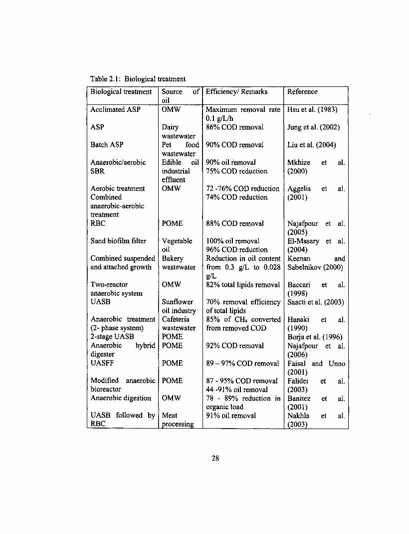
Table 2.1: Biological treatment
Biological treatment Source of oil
Efficiency! Remarks Reference
Acclimated ASP OMW Maximum removal rate Hsu et al. (1983) 0.1 g/L/h
ASP Dairy wastewater
86% COD removal Jung et al. (2002)
Batch ASP Pet food wastewater
90% COD removal Liu et al. (2004)
Anaerobic/aerobic Edible oil 90% oil removal Mkhize et al. SBR industrial
effluent 75% COD reduction (2000)
Aerobic treatment OMW 72 -76% COD reduction Aggelis et al. Combined anaerobic-aerobic treatment
74% COD reduction (2001)
RBC POME 88% COD removal Najafpour et al. (2005)
Sand biofilm filter Vegetable 100% oil removal El-Masary et al. oil 96% COD reduction (2004)
Combined suspended Bakery Reduction in oil content Keenan and and attached growth wastewater from 0.3 g/L to 0.028 Sabelnikov (2000)
Two-reactorTwo-reactor anaerobic system
OMW -
82% total lipids removal Baccari et al. (1998)
UASB Sunflower oil industry
70% removal efficiency of total lipids
Saacti et al. (2003)
Anaerobic treatment Cafeteria 85% of CH4 converted Hanaki et al. (2- phase system) wastewater from removed COD (1990) 2-stage UASB POME Borja et al. (1996) Anaerobic hybrid digester
POME 92% COD removal Najafpour et al. (2006)
UASFF POME 89 — 97% COD removal Faisal and Unno (2001)
Modified anaerobic POME 87 - 95% COD removal Falidei et al. bioreactor 44 -91% oil removal (2003) Anaerobic digestion OMW 78 - 89% reduction in
organic load Banitez et al. (2001)
UASB followed by Meat 91% oil removal Nakhla et al. RBC processing (2003)
28
Table 2.1: Biological treatment
Biological treatment Source of oil
Efficiency/ Remarks Reference
Acclimated ASP OMW Maximum removal rate Hsu et al. (1983) 0.1 g/L/h
ASP Dairy 86% COD removal Jung et al. (2002) wastewater
Batch ASP Pet food 90% COD removal Liu et al. (2004) wastewater
Anaerobic/aerobic Edible oil 90% oil removal Mkhize et al. SBR industrial 75% COD reduction (2000)
effluent Aerobic treatment OMW 72 -76% COD reduction Aggelis et al. Combined 74% COD reduction (2001) anaerobic-aerobic treatment RBC POME 88% COD removal Najafpour et al.
(2005) Sand biofilm filter Vegetable 100% oil removal El-Masary et al.
oil 96% COD reduction (2004) Combined suspended Bakery Reduction in oil content Keenan and and attached growth wastewater from 0.3 g/L to 0.028 Sabelnikov (2000)
g/L Two-reactor OMW 82% total lipids removal Baccari et al. anaerobic system (1998) UASB Sunflower 70% removal efficiency Saacti et al. (2003)
oil industry of total lipids Anaerobic treatment Cafeteria 85% of CH> converted Hanaki et al. (2- phase system) wastewater from removed COD (1990) 2-stage UASB POME Boija et al. (1996) Anaerobic hybrid POME 92% COD removal Najafpour et al. digester (2006) UASFF POME 89 - 97% COD removal Faisal and Unno
(2001) Modified anaerobic POME 87 - 95% COD removal Falidei et al. bioreactor 44-91% oil removal (2003) Anaerobic digestion OMW 78 - 89% reduction in Banitez et al.
organic load (2001) UASB followed by Meat 91% oil removal Nakhla et al. RBC processing (2003)
28
catalyze the hydrolysis of complex organic compounds, transforming them into
substances which can be readily biodegraded by the microbial consortium present in
subsequent biological treatments (Cammarota and Freire 2006). However, the use of
enzyme preparations is not attractive due to the fact it is only used for the hydrolysis of
oils to fatty acids and glycerol (Malcata et al. 1992; Paiva et al. 2000). The liberated fatty
acids can form colloidal particles that aggregate and precipitate from solutions during
changes in environmental conditions during the treatment system, causing clogging and
process failure (Chao and Yang 1981). Therefore, this approach provides only a partial
solution to the problem. Process stability may also depend upon the state of the added
enzyme preparations. If added to a solution, enzymes would disappear from the system. It
is also difficult to recover enzymes from reactor effluent at the end of the catalytic
process, which is an even more expensive exercise. In contrast, immobilized enzymes
would be retained within the system and most likely would improve stability in relation
to environmental conditions (Malcata et al. 1992). Immobilized enzymes have the
advantages of multiple usage, controlled reactions, and mechanical stability (Murray et
al. 1997). Despite the advantages, the use of immobilized enzymes in wastewater
treatment has been limited by several factors, mainly due to the high cost of the enzymes
connected with the immobilization procedure. Also, loss of enzyme activity during the
immobilization procedure and during the reaction is the main hurdle in the way of
widespread commercialization (Murray et al. 1997).
In a study conducted by Jeganathan et al. (2006), hydrolysis of oil originating
from pet food industrial wastewater was evaluated. Lipase from Candida rugosa was
29

immobilized and applied into the hydrolysis experiment. Lipase from Candida rugosa is
a microbial enzyme produced by the fermentation of yeasts. It was extensively used for
oil hydrolysis (Murray et al. 1997; Knezeric et al. 1998; Murthy et al. 2004) because it is
one of the commercially available lipases that have the ability to liberate all types of acyl
chains. The study showed approximately 50% of oil was hydrolyzed due to enzyme
activity. A significant increment in COD and VFA production was also observed. During
the 3-day experiment, approximately 65% of the beads were recovered and
approximately 70% of the enzyme activity remained in the beads after hydrolysis. The
study showed the immobilized lipase could be used up to 4 cycles with a 55% activity
recovery. However, after 4 cycles, the activity loss was critical, probably due to lipase
leakage from the beads and/or blockage of substrate/product. The study showed the
potential of immobilized lipase as a pre-treatment step in the biological treatment of pet
food manufacturing wastewater.
Jung et al. (2002) treated dairy wastewater in a batch activated sludge system with
and without an enzymatic pre-hydrolysis stage. A fermented babassu cake containing
Penicillium restrictum lipase was used in the pre-hydrolysis stage. The efficiency of pre-
hydrolysis was monitored via the formation of free acids. During the study, a marked
difference between the concentration of free acids, before and after hydrolysis, was
observed, indicating a modification in composition of wastewater even when a small
quantity of fermented cake (0.2) was utilized. Following enzymatic hydrolysis, COD
values were observed to rise due to the presence of organic compounds other than
microorganisms and proteins in the enzymatic cake. Although fed with high COD
30
concentrations, the hydrolyzed bioreactor maintained COD removal efficiencies in the
range of 82% to 93%, indicating that products of enzymatic hydrolysis were easily
metabolized by the microbial consortium present in the activated sludge. Also, biomass
growth was observed to be more intense in the hydrolyzed bioreactor.
Leal et al. (2006) conducted a study regarding the biological treatment of dairy
wastewater containing high levels of oil. The study used two identical Upflow Anaerobic
Sludge Blanket (UASB) reactors, one fed with wastewater from an upstream enzymatic
hydrolysis step and the other with raw wastewater. Hydrolysis was carried out at 35°C for
14 hours using an enzyme prepared via solid-state fermentation, showing pronounced
lipase activity. The UASB reactor fed with the hydrolyzed wastewater assimilated the
increase of oil content in the influent and showed stable COD removal even when the oil
concentration was raised to 1000 mg/L. Dharmshiti and Kuhasuntisuk (1998)
investigated the effect of the addition of lipase to a biological system treating restaurant
wastewater. The oil content was totally removed after 48 hours of incubating the
wastewater with the enzyme. However, the amount of enzyme preparation used in the
study was appreciably high. Cammarota and Freire (2006) first proposed hydrolysis of oil
by solid preparation of lipase using dairy wastewater. The results of the work showed that
pre-treatment with enzymatic hydrolysis improved the treatment of dairy wastewater in a
bench scale UASB reactor. Leal et al. (2002) carried out a similar work using a liquid
enzyme and batch operated anaerobic reactors. The highest level of oil investigated by
the authors was 1200 mg/L and the removal attained in reactors fed with the hydrolyzed
stream was significantly higher than that reached in the control reactor without pre-
31

treatment. Therefore, enzymatic pre-treatment was found to improve the performance of
anaerobic reactors, which treat industrial wastewaters containing high oil concentrations.
Gombert et al. (1999) studied lipase production by Penicillium restrictum in solid-state
fermentation using a babassu oil cake as a substrate. The highest lipase activity was
observed after 24 hours of cultivation with 2% olive oil enrichment.
2.2.2 Microbial Degradation of Oils
Generally, microbial oil degradation is considered to occur as a result of
hydrolysis of oil by secretion of lipase, an oil-degrading enzyme, which degrades the oil
to organic acids and Volatile Fatty Acids (VFA) via beta-oxidation, a fatty acid
degradation pathway. Finally, oil is decomposed to CO2 and H2O (Taken et al. 2005).
Keenan and Sabelnikov (2000) studied the biodegradation of corn, olive, sunflower and
waste oils employing a variety of bacterial strains such as Acinetobacter sp.,
Rhodococcus sp. and Caseobacter sp. that were isolated from different environments
based on their ability to grow on vegetable and waste oils and by commercial bacterial
preparations specifically designed for oil degradation. As for all bacterial strains and
preparations, only corn oil and waste oils supported microbial growth more efficiently
than either olive or sunflower oil. Moreover, the Caseobacter strain and one commercial
preparation could not grow on olive oil at all. Wakelin and Forster (1997) reported
similar results regarding the Acinetobacter strain, which was found to grow efficiently on
oils including Rhodococcus rubra, Nocardia amarae, and Microthrix parvicella.
However, even Acinetobacter sp. could not reduce the content of lipids in wastewater to
32
treatment. Therefore, enzymatic pre-treatment was found to improve the performance of
anaerobic reactors, which treat industrial wastewaters containing high oil concentrations.
Gombert et al. (1999) studied lipase production by Penicillium restrictum in solid-state
fermentation using a babassu oil cake as a substrate. The highest lipase activity was
observed after 24 hours of cultivation with 2% olive oil enrichment.
2.2.2 Microbial Degradation of Oils
Generally, microbial oil degradation is considered to occur as a result of
hydrolysis of oil by secretion of lipase, an oil-degrading enzyme, which degrades the oil
to organic acids and Volatile Fatty Acids (VFA) via beta-oxidation, a fatty acid
degradation pathway. Finally, oil is decomposed to CO2 and H2O (Takeno et al. 2005).
Keenan and Sabelnikov (2000) studied the biodegradation of com, olive, sunflower and
waste oils employing a variety of bacterial strains such as Acinetobacter sp.,
Rhodococcus sp. and Caseobacter sp. that were isolated from different environments
based on their ability to grow on vegetable and waste oils and by commercial bacterial
preparations specifically designed for oil degradation. As for all bacterial strains and
preparations, only corn oil and waste oils supported microbial growth more efficiently
than either olive or sunflower oil. Moreover, the Caseobacter strain and one commercial
preparation could not grow on olive oil at all. Wakelin and Forster (1997) reported
similar results regarding the Acinetobacter strain, which was found to grow efficiently on
oils including Rhodococcus rubra, Nocardia amarae, and Microthrix parvicella.
However, even Acinetobacter sp. could not reduce the content of lipids in wastewater to
values lower than 0.1 g/L. From an initial oil content of 1.5 g/L, the lowest values
achieved using Acinetobacter sp. were 0.35 g/L for corn oil and 0.267 g/L for waste oil.
Keenan and Sabelnikov (2000) also reported that microbial growth was more so on
unrefined oils than on refined oils; this was likely because the former contained nutrients,
which were removed while making refined oil.
In a study carried out by El-Bestawy et al. (2005), eight bacterial species were
isolated from vegetable oil contaminated industrial wastewater, four of which were found
to have the ability to degrade oil in the contaminated wastewater. The isolates were
identified as Pseudomonas sp., P. diminuta, P. Pseudoalcaligenes and Escherichia sp.
Results showed that all tested bacteria were able to degrade palm oil completely and
utilized free fatty acids as a carbon source. The combination, Pseudomonas sp. and P.
diminuta, produced the highest degradative activity followed by combination,
Pseudomonas sp., P. diminuta and P. Pseudoalcaligenes. Also, the combination of
Pseudomonas sp. and P. diminuta produced the highest activity in reducing COD by 93%
and BOD by 100%.
An inoculum containing a mixed culture of fifteen bacterial isolates from various
fatty wastewater samples was developed by Tano-Debrah et al. (1999) to degrade oils.
The inoculum was effective in wastewaters with pH ranging from 4.5 to 9.5 and the
optimum treatment temperature was 20 — 25°C. It was observed that the growth of
organisms was better in an alkaline medium due to better emulsification. Microorganisms
generally live at the oil-water interfaces and the attack on oil molecules and microbial
oxidation is rapid when the hydrocarbon molecule is in intimate contact with water at
33
values lower than 0.1 g/L. From an initial oil content of 1.5 g/L, the lowest values
achieved using Acinetobacter sp. were 0.35 g/L for corn oil and 0.267 g/L for waste oil.
Keenan and Sabelnikov (2000) also reported that microbial growth was more so on
unrefined oils than on refined oils; this was likely because the former contained nutrients,
which were removed while making refined oil.
In a study carried out by El-Bestawy et al. (2005), eight bacterial species were
isolated from vegetable oil contaminated industrial wastewater, four of which were found
to have the ability to degrade oil in the contaminated wastewater. The isolates were
identified as Pseudomonas sp., P. diminuta, P. Pseudoalcaligenes and Escherichia sp.
Results showed that all tested bacteria were able to degrade palm oil completely and
utilized free fatty acids as a carbon source. The combination, Pseudomonas sp. and P.
diminuta, produced the highest degradative activity followed by combination,
Pseudomonas sp., P. diminuta and P. Pseudoalcaligenes. Also, the combination of
Pseudomonas sp. and P. diminuta produced the highest activity in reducing COD by 93%
and BOD by 100%.
An inoculum containing a mixed culture of fifteen bacterial isolates from various
fatty wastewater samples was developed by Tano-Debrah et al. (1999) to degrade oils.
The inoculum was effective in wastewaters with pH ranging from 4.5 to 9.5 and the
optimum treatment temperature was 20 - 25°C. It was observed that the growth of
organisms was better in an alkaline medium due to better emulsification. Microorganisms
generally live at the oil-water interfaces and the attack on oil molecules and microbial
oxidation is rapid when the hydrocarbon molecule is in intimate contact with water at
33

temperatures ranging from 15 to 35*C, which means adequate mixing or dispersion of the
water and oil is necessary for effective degradation. Adequate mixing occurs in emulsion
formation. Biodegradative tests with the inoculum on samples of eight different oils,
developed by Tano-Debrah et al. (1999), showed that the organisms in the culture could
degrade several oils of plant and animal origin.
Takeno et al. (2005) studied the removal of cooking oil from domestic
wastewater. A continuous treatment of oil containing wastewater was carried out with
agar-immobilized Rhodobacter Shaeroide S, a photosynthetic bacterium, at a fixed
dilution rate of 0.4 /day. The results indicated that 96% of the oil was removed from the
wastewater, and the maximum removal rate of oil reached approximately 3.83 kg
oil/m3/day. The study showed that immobilized photosynthetic bacteria directly
decomposed one part of the oil contained in the wastewater, while oil-decomposing
bacteria (naturally growing Pseudomonas and Bacillus) decomposed another part of the
oil, degrading it to organic fatty acids such as propionic and acetic acid. Photosynthetic
bacteria consumed these acids. As a result, oil degradation was promoted by the addition
of photosynthetic bacteria and the combination showed significant decomposition of oil
from wastewater.
Prasertasan et al. (2004) investigated the bioseparation of suspended solids and oil
from POME. Two thermotolerant lipase producing fungal isolates, ST4 and ST29, were
observed to remove 98.9% and 88.9% of oil, respectively. The high treatment efficiency
was found to be the consequence of the entrapment of the majority of suspended solids
and residual oil of POME in the polymer excreted from these strains. Lipases are widely
34
temperatures ranging from 15 to 35°C, which means adequate mixing or dispersion of the
water and oil is necessary for effective degradation. Adequate mixing occurs in emulsion
formation. Biodegradative tests with the inoculum on samples of eight different oils,
developed by Tano-Debrah et al. (1999), showed that the organisms in the culture could
degrade several oils of plant and animal origin.
Takeno et al. (2005) studied the removal of cooking oil from domestic
wastewater. A continuous treatment of oil containing wastewater was carried out with
agar-immobilized Rhodobacter Shaeroide S, a photosynthetic bacterium, at a fixed
dilution rate of 0.4 /day. The results indicated that 96% of the oil was removed from the
wastewater, and the maximum removal rate of oil reached approximately 3.83 kg
oil/m3/day. The study showed that immobilized photosynthetic bacteria directly
decomposed one part of the oil contained in the wastewater, while oil-decomposing
bacteria (naturally growing Pseudomonas and Bacillus) decomposed another part of the
oil, degrading it to organic fatty acids such as propionic and acetic acid. Photosynthetic
bacteria consumed these acids. As a result, oil degradation was promoted by the addition
of photosynthetic bacteria and the combination showed significant decomposition of oil
from wastewater.
Prasertasan et al. (2004) investigated the bioseparation of suspended solids and oil
from POME. Two thermotolerant lipase producing fungal isolates, ST4 and ST29, were
observed to remove 98.9% and 88.9% of oil, respectively. The high treatment efficiency
was found to be the consequence of the entrapment of the majority of suspended solids
and residual oil of POME in the polymer excreted from these strains. Lipases are widely
34

produced in fungi and their production and activity in organisms such as Rhizopus,
Mucor and Aspergillus, have been well studied (Jensen 1971; Akhtar et al. 1980; Chopra
and Khuller 1983). In a study conducted by Gopinath et al. (2005) on thirty-four wild
fungal species associated with edible oil mill waste, the species Absidia colymbifera,
Aspergillus fumigatus, Aspergillus japonicus, Aspergillus nidulans, Aspergillus terreus,
Cunninghamella verticillata, Curvularia pallescens, Fusarium oxysporum, Geotrichum
candidum, Mucor racemosus, Penicillium citrinum, Penicillium frequentans, Rhizopus
stolonifer, and Trichoderma viride were found to exhibit maximum lipase activity. The
literature advises that lipase-producing fungi can utilize oil as a main carbon source,
which has approximately twice the energy value of glucose, and are capable of reducing
the COD of oil effluent (Koritala et al. 1987; Ratledge 1992). When fungi are confronted
with fats and oils in a growth medium, triacylglycerol is hydrolyzed by fungal lipases to
yield diacylglycerol, monoacylglycerols, free fatty acids and glycerol.
Mucor circinelloides was found to effectively degrade a laboratory-based
sunflower oil waste (Joseph et al. 2005). The fungus was found to exhibit a preference
towards the utilization of unsaturated fatty acids in the presence of acetate. The study
suggested that fungi could be used in oil waste removal while, at the same time, biomass,
rich in essential fatty acids such as linoleic acid and GLA, can also be produced. Fabritius
et al. (1998) studied bioconversions of sunflower oil and rapeseed oil in fed-batch
cultures fermented with Candida tropicalis. Co-fermentations with palmitic acid resulted
in successful transformations to different 3- hydroxydioic acids.
35
produced in fungi and their production and activity in organisms such as Rhizopus,
Mucor and Aspergillus, have been well studied (Jensen 1971; Akhtar et al. 1980; Chopra
and Khuller 1983). In a study conducted by Gopinath et al. (2005) on thirty-four wild
fungal species associated with edible oil mill waste, the species Absidia corymbifera,
Aspergillus fumigatus, Aspergillus japonicus, Aspergillus nidulans, Aspergillus terreus,
Cunninghamella verticillata, Curvularia pallescens, Fusarium oxysporum, Geotrichum
candidum, Mucor racemosus, Penicillium citrinum, Penicillium frequentans, Rhizopus
stolonifer, and Trichoderma viride were found to exhibit maximum lipase activity. The
literature advises that lipase-producing fungi can utilize oil as a main carbon source,
which has approximately twice the energy value of glucose, and are capable of reducing
the COD of oil effluent (Koritala et al. 1987; Ratledge 1992). When fungi are confronted
with fats and oils in a growth medium, triacylglycerol is hydrolyzed by fungal lipases to
yield diacylglycerol, monoacylglycerols, free fatty acids and glycerol.
Mucor circinelloides was found to effectively degrade a laboratory-based
sunflower oil waste (Joseph et al. 2005). The fungus was found to exhibit a preference
towards the utilization of unsaturated fatty acids in the presence of acetate. The study
suggested that fungi could be used in oil waste removal while, at the same time, biomass,
rich in essential fatty acids such as linoleic acid and GLA, can also be produced. Fabritius
et al. (1998) studied bioconversions of sunflower oil and rapeseed oil in fed-batch
cultures fermented with Candida tropicalis. Co-fermentations with palmitic acid resulted
in successful transformations to different 3- hydroxydioic acids.
35

The ability of Aspergillus fumigatus Fres. and Aspergillus nidulans (Eidam) wint,
from Nigerian palm products, to degrade vegetable oils was examined (Ogundero 1982).
Both species were found to readily hydrolyze palm oil and palm kernel oil and good
growth was recorded with respect to triglycerides, which were used as a source of carbon.
Extracellular lipases were detected and found to be active at a pH level of 5.6. Barker and
Worgan (1981) investigated the growth of Aspergillus oryzae on palm oil effluent. The
fungus grew in a batch culture indicating the utilization of principal substrate
components, followed by a period of protein assimilation and then, lipid and
carbohydrate utilization. Supplementation with an inorganic nitrogen source was found to
be necessary and BOD reductions of 75% and COD reductions of 75% to 80% were
observed in batch cultures.
Aspergillus niger was observed to posses extracellular enzymes that hydrolyze
pectins, polyphenols and tannins. It degrades many phenolic compounds and can be used
in the pretreatment of olive black water (Hamdi et al. 1991). The organic fraction of olive
oil mill waste includes sugars, tannins, polyphenols, polyalcohols, pectins and lipids
(Hamdi 1993). Hamdi et al. (1991) observed a reduction in COD of 52.5% using A. niger
in aerobic conditions. Average COD removals of 55%, 52.5% and 62.8% in olive mill
wastewater, fermented with Geotrichium sp, Aspergillus sp, Candida tropicalis,
respectively, were observed by Fadil et al. (2003). Under optimum conditions, C.
versicolor and F. trogii removed 63% and 70% of COD, respectively (Yesilada et al.
1998). The addition of sulphate, glucose and nitrogen had no effect upon biodegradation
and immobilized fungi in calcium alginate gels, obtained at high yields. In a study
36

conducted by Yesilada et al. (1999), while treating OMW aerobically with fungi, it was
found that Coriolus versicolor, Funalia trogii and Pleurotus sarorcaju showed high
reductions in COD. The ability of Phanerochaete chrysosporium to degrade the phenolic
compounds of olive oil mill wastewater, using cells immobilized on loofah, was
examined by Ahmadi et al. (2006). The fungus did not grow on the concentrated
wastewater and a reduction in COD of 5% was observed. Pleurotus ostreatus grown in
bioreactor batch cultures in a model OMW (diluted and sterilized) was observed to cause
significant phenolic removal (Aggelis et al. 2003). Laccase, the sole ligninolytic enzyme
detected in the growth environment, was found during primary metabolic growth. The
toxicity of OMW against the seeds of Lepidium sativum and the marine Branchiopoda
Artemia sp. was observed to decrease after biotreatment. Pleurotus ostreatus was able to
reduce phenolic content and the toxicity of sterilized OMW, in bioreactor cultures.
During a study carried out by Zheng et al. (2003) regarding the treatment of salad oil
manufacturing wastewater, using yeast isolates, a large loss of biomass was observed
which subsequently reduced the treatment efficiency. Of the five yeast species used in the
study, only Candida tropicalis remained in the aeration tank, possibly because it had
better settleability. An addition of nitrogen to the final effluent stimulated the activity of
this yeast, which resulted in treatment efficiency similar to that of the mixed yeast
system. Lanciotti et al. (2005) examined the ability of different Yarrowia lipolytica yeast
strains to grow in OMW and to reduce its COD level. Results showed that several
Yarrowia lipolytica strains are good candidates for the reduction of the pollution potential
of OMW and for the production of enzymes and metabolites such as lipase and citric
37

acid. In another study conducted on Yarrowia lipolytica, it was observed that the yeast
reduced the COD level of OMW by 80% and produced a useful biomass and enzyme
lipase (Sciolli and Vollaro 1997).
2.2.2.1 Biodegradation of Oil under Thermophilic Conditions
At temperatures above 50°C, the oil aggregates melt, and stable emulsions of
substrates with large surface areas are formed during agitation. Under such conditions,
the bioavailability of such hydrophobic substrates for enzymes and microorganisms is
significantly increased. From a technological point of view, high temperatures are
desirable, because the viscosity of the streams decrease, and thus, diffusion and mass
transfer are accelerated (Becker et al. 1999). The biological treatment of oils under
thermophilic conditions, i.e., above 60 °C, is expected to be advantageous due to
favorable changes in physical properties of the hydrophobic compounds with increasing
temperature.
Becker et al. (1999) studied the aerobic thermophilic degradation of olive oil
using a pure culture of bacterial strain, Bacillus thermoleovorans 1111-91, in a
continuously operated stirred tank reactor. It was observed that an oil removal of more
than 90% of the initial oil concentration of 2 g/L was obtained at a residence time of 2
hours. A relatively high maximum biomass yield of 1.05 g dry cell per g of olive oil
consumed was measured in the study. A severe growth inhibition was observed when the
feed olive oil concentration was increased to more than 4 g/L. Compared with data from
mesophilic processes, the oil degradation rates obtained under thermophilic conditions,
38
acid. In another study conducted on Yarrowia lipolytica, it was observed that the yeast
reduced the COD level of OMW by 80% and produced a useful biomass and enzyme
lipase (Sciolli and Vollaro 1997).
2.2.2.1 Biodegradation of Oil under Thermophilic Conditions
At temperatures above 50°C, the oil aggregates melt, and stable emulsions of
substrates with large surface areas are formed during agitation. Under such conditions,
the bioavailability of such hydrophobic substrates for enzymes and microorganisms is
significantly increased. From a technological point of view, high temperatures are
desirable, because the viscosity of the streams decrease, and thus, diffusion and mass
transfer are accelerated (Becker et al. 1999). The biological treatment of oils under
thermophilic conditions, i.e., above 60 °C, is expected to be advantageous due to
favorable changes in physical properties of the hydrophobic compounds with increasing
temperature.
Becker et al. (1999) studied the aerobic thermophilic degradation of olive oil
using a pure culture of bacterial strain, Bacillus thermoleovorans IHI-91, in a
continuously operated stirred tank reactor. It was observed that an oil removal of more
than 90% of the initial oil concentration of 2 g/L was obtained at a residence time of 2
hours. A relatively high maximum biomass yield of 1.05 g dry cell per g of olive oil
consumed was measured in the study. A severe growth inhibition was observed when the
feed olive oil concentration was increased to more than 4 g/L. Compared with data from
mesophilic processes, the oil degradation rates obtained under thermophilic conditions,

were extremely high. Lapara and Alleman (1999) attributed this difference to the fact that
nitrifying bacteria, floc-forming organisms and higher organisms that aid flocculations
were not present, which affected sludge sedimentation. Markossian et al. (2000) carried
out a study regarding the same strain, Bacillus thermoleovorans IHI-91, and observed
that the aerobic bacterium grew optimally at 65°C with a pH of 6.0 and secreted a high
level of lipase. The strain was observed to utilize several oils such as olive oil, sunflower
oil, soya oil, and fish oil as sole carbon and energy sources without an additional supply
of growth factors. A degradation of about 93% of triolein, which is present in olive oil,
was observed after only 7 hours of fermentation, at a maximal growth rate of 1.0 /h. Due
to its production of high concentrations of thermoactive lipases and esterases, the
bacterium was found to be capable of degrading a wide range of oils at high
temperatures. Results related to the microbial degradation of oil from wastewater are
summarized in Table 2.2.
2.2.3 Removal of Oil by Various Sorbents
In the past, many sorbents such as activated carbon, peat, bentonit, and
organoclay have been used to remove oil from wastewater. Activated carbon is an •
adsorbent that is commonly used in the removal of a wide variety of organic compounds
including oil from water (Ahmad et al. 2005b; Alther 1995; Alther 1996; Mathavan and
Viraraghavan 1989; Viraraghavan and Moazed 2003; Zunan et al. 1995). The
disadvantage of using activated carbon in removing oil from water is that emulsified oil
can bind its pore spaces during operation (Mysore et al. 2006).
39
were extremely high. Lapara and Alleraan (1999) attributed this difference to the fact that
nitrifying bacteria, floc-forming organisms and higher organisms that aid flocculations
were not present, which affected sludge sedimentation. Markossian et al. (2000) carried
out a study regarding the same strain, Bacillus thermoleovorans IHI-91, and observed
that the aerobic bacterium grew optimally at 65°C with a pH of 6.0 and secreted a high
level of lipase. The strain was observed to utilize several oils such as olive oil, sunflower
oil, soya oil, and fish oil as sole carbon and energy sources without an additional supply
of growth factors. A degradation of about 93% of triolein, which is present in olive oil,
was observed after only 7 hours of fermentation, at a maximal growth rate of 1.0 /h. Due
to its production of high concentrations of thermoactive lipases and esterases, the
bacterium was found to be capable of degrading a wide range of oils at high
temperatures. Results related to the microbial degradation of oil from wastewater are
summarized in Table 2.2.
2.2.3 Removal of Oil by Various Sorbents
In the past, many sorbents such as activated carbon, peat, bentonit, and
organoclay have been used to remove oil from wastewater. Activated carbon is an
adsorbent that is commonly used in the removal of a wide variety of organic compounds
including oil from water (Ahmad et al. 2005b; Alther 1995; Alther 1996; Mathavan and
Viraraghavan 1989; Viraraghavan and Moazed 2003; Zunan et al. 1995). The
disadvantage of using activated carbon in removing oil from water is that emulsified oil
can bind its pore spaces during operation (Mysore et al. 2006).

Table 2.2: Microbial degradation
Microorganism Source Efficiency/ Remarks Reference
Acinetobacter sp. Rhodococcus sp.
Corn, olive, sunflower and
Corn and waste oil supported all bacterial
Keenan and Sabelnikov
Caseobacter sp. waste oils strains than olive and
(2000) sunflower oil
Acinetobacter P. Corn and waste oil
Reduce lipid content from 1.5 g/L to 0.35 g/L for corn and to 0.267 g/L for waste oil.
Wakelin and Forster (1997)
Pseudomonas sp. Pseudomonas sp. And P. diminuta P. pseudoalcaligens Vegetable oil P. diminuta combined,
reduced COD by 93% and El-Bestawy et al. (2005)
Escherichia sp. BOD by 100% Rhodobacter Domestic Takeno et al. shaeroide S wastewater
96% oil removal (2005)
Mucor circinelloides Sunflower oil waste
Presence of acetate enhanced sunflower oil utilization
Joseph et al. (2005)
Aspergillus fumigatus Aspergillus nidulans
Vegetable oils Hydrolyze palm and palm kernel oil
Ogundero (1982)
Barker and Aspergillus oryzae POME 75-80% COD reduction Worgan
(1981)
Aspergillus niger OMW 52.5% COD reduction Hamdi et al. (1991)
C. versicolor OMW
63% COD reduction Yesilada et F. trogii 70% COD reduction al. (1998) C. versicolor F. trogii P. sarorcaju
OMW High COD reduction Yesilada et al. (1999)
Phanerochaete chlysosporium OMW 50% COD reduction Ahmadi et al.
(2006) Scioli and Vollaro
Yarrowia lipolytica OMW 80% COD reduction (1997); Lanciotti et al. (2005)
40
Table 2.2: Microbial degradation
Microorganism Source Efficiency/ Remarks Reference
Acinetobacter sp. Rhodococcus sp. Caseobacter sp.
Acinetobacter sp.
Pseudomonas sp. P. diminuta P. pseudoalcaligens Escherichia sp. Rhodobacter shaeroide S
Mucor circinelloides
Aspergillus fumigatus Aspergillus nidulans
Aspergillus oryzae
Aspergillus niger
C. versicolor F. trogii C. versicolor F. trogii P. sarorcaju Phanerochaete chrysosporium
Yarrowia lipolytica
Corn, olive, sunflower and waste oils
Corn and waste oil
Vegetable oil
Domestic wastewater
Sunflower oil waste
Vegetable oils
POME
OMW
OMW
OMW
OMW
OMW
Corn and waste oil supported all bacterial strains than olive and sunflower oil Reduce lipid content from 1.5 g/L to 0.35 g/L for corn and to 0.267 g/L for waste oil. Pseudomonas sp. And P. diminuta combined, reduced COD by 93% and BOD by 100%
96% oil removal
Presence of acetate enhanced sunflower oil utilization
Hydrolyze palm and palm kernel oil
75-80% COD reduction
52.5% COD reduction
63% COD reduction 70% COD reduction
High COD reduction
50% COD reduction
80% COD reduction
Keenan and Sabelnikov (2000)
Wakelin and Forster (1997)
El-Bestawy et al. (2005)
Takeno et al. (2005)
Joseph et al. (2005)
Ogundero (1982)
Barker and Worgan (1981) Hamdi et al. (1991) Yesilada et al. (1998)
Yesilada et al. (1999)
Ahmadi et al. (2006) Scioli and Vollaro (1997); Lanciotti et al. (2005)
40

Crushed and/or processed plant materials have been used to adsorb oil from surfaces for
some time. For example, cotton linters, crushed corncobs and modified pulp have been
investigated (Johnson et al. 1973; Silva-Tilak 2002; Sun et al. 2002). Deschamps et al.
(2003) used cotton as a bed material to recover oil from oily water and found the oil—
water separation could be improved at a lower temperature, lower flow, a deeper bed
material and larger oil drop. Mathavan and Viraraghavan (1992) used horticultural peat
as a bed material to examine the capability of the filter bed in oily water clean-up.
Moazed and Viraraghavan (2002) examined the ability of an anthracite/organoclay
mixture in removing oil from water. Varghese and Cleveland (1998) studied the
feasibility of using a kenaf-filled filter in removing oil from a surfactant-stabilized oil-in
water emulsion. The possibilities of reed canary grass, flax and hemp fiber as oil
absorbing filter materials were investigated by Pasila (2004). It was found that these
materials were able to separate oil from water during the filtration of oily water.
Oil removal efficiencies of 98.2%, 46.3%, 86.5%, 98.2 %, 99.2%, 92.4%, and
94.2% were obtained for peat, coal, sand, amberlite, activated carbon, polypropylene, and
fiberglass, respectively (Viraraghavan and Mathavan 1990). Sodium bentonite was found
to be effective in removing oil and efficiencies of 88-94% for Standard Mineral Oil
(SMO), 85-96% and 87-96% for two cutting oils, 84-86% for produced water from
production wells, and 54-87% for refinery effluent were obtained (Viraraghavan and
Moazed 2003). Moazed and Viraraghavan (2001) showed that bentonite organo-
clay/anthracite were quite effective in breaking down a number of oil-in-water emulsions.
In a recent study, Ahmad et al. (2005a) investigated adsorption of residue oil from Palm
41
Crushed and/or processed plant materials have been used to adsorb oil from surfaces for
some time. For example, cotton linters, crushed corncobs and modified pulp have been
investigated (Johnson et al. 1973; Silva-Tilak 2002; Sun et al. 2002). Deschamps et al.
(2003) used cotton as a bed material to recover oil from oily water and found the oil-
water separation could be improved at a lower temperature, lower flow, a deeper bed
material and larger oil drop. Mathavan and Viraraghavan (1992) used horticultural peat
as a bed material to examine the capability of the filter bed in oily water clean-up.
Moazed and Viraraghavan (2002) examined the ability of an anthracite/organoclay
mixture in removing oil from water. Varghese and Cleveland (1998) studied the
feasibility of using a kenaf-filled filter in removing oil from a surfactant-stabilized oil-in
water emulsion. The possibilities of reed canary grass, flax and hemp fiber as oil
absorbing filter materials were investigated by Pasila (2004). It was found that these
materials were able to separate oil from water during the filtration of oily water.
Oil removal efficiencies of 98.2%, 46.3%, 86.5%, 98.2 %, 99.2%, 92.4%, and
94.2% were obtained for peat, coal, sand, amberlite, activated carbon, polypropylene, and
fiberglass, respectively (Viraraghavan and Mathavan 1990). Sodium bentonite was found
to be effective in removing oil and efficiencies of 88-94% for Standard Mineral Oil
(SMO), 85-96% and 87-96% for two cutting oils, 84—86% for produced water from
production wells, and 54-87% for refinery effluent were obtained (Viraraghavan and
Moazed 2003). Moazed and Viraraghavan (2001) showed that bentonite organo-
clay/anthracite were quite effective in breaking down a number of oil-in-water emulsions.
In a recent study, Ahmad et al. (2005a) investigated adsorption of residue oil from Palm
41

Oil Mill Effluent (POME) using chitosan from crab shells. Chitosan was found to remove
almost 99% of residue oil from POME. Chitosan, in powder form, had a higher capacity
for residue oil compared to the flake form. Several of the physicochemical parameters of
adsorption were evaluated at dynamic and equilibrium conditions. The results of this
study can be useful with respect to further applications in treatments of oily wastewaters
(Ahmad et al. 2005a). Studies have been conducted to evaluate the use of walnut shell
filters as an alternative to conventional sand filters to remove free oils and suspended
solids (Blumenschein et al. 2001). USFilter Zimpro products, USA have developed an
Auto-Shell Walnut shell filter to remove oily contaminants from water (USFilter
Corporation 2005). The walnut shell media was found to have good oil adsorbent ability
and low media gravity (Yang et al. 2002). The media have been observed to be tough
enough to maintain their size during the back washing operation, thereby reducing
possible loss during the filtration process (Rahman 1992). Srinivasan and Viraraghavan
(2008) conducted batch kinetic studies to evaluate the equilibrium time required by
walnut shell media to sorb oil. As for pure oil medium, sorption capacities of 0.30 g/g,
0.51 g/g and 0.58 g/g were obtained for standard mineral oil, canola oil and Bright- Edge
oil, respectively. Walnut shells remove oil by coalescing oil droplets but do not bind with
them. Similar sorption capacity tests have been conducted by Mysore et al. (2004) on
vermiculite for both pure oil and oil on aqueous medium. The external surface of the
hydrophobic vermiculite had a wax coating, which resulted in adsorption followed by
absorption of oil (Mysore et al. 2004). Oil sorption capacity values of different materials
are provided in Table 2.3.
42
Oil Mill Effluent (POME) using chitosan from crab shells. Chitosan was found to remove
almost 99% of residue oil from POME. Chitosan, in powder form, had a higher capacity
for residue oil compared to the flake form. Several of the physicochemical parameters of
adsorption were evaluated at dynamic and equilibrium conditions. The results of this
\
study can be useful with respect to further applications in treatments of oily wastewaters
(Ahmad et al. 2005a). Studies have been conducted to evaluate the use of walnut shell
filters as an alternative to conventional sand filters to remove free oils and suspended
solids (Blumenschein et al. 2001). USFilter Zimpro products, USA have developed an
Auto-Shell Walnut shell filter to remove oily contaminants from water (USFilter
Corporation 2005). The walnut shell media was found to have good oil adsorbent ability
and low media gravity (Yang et al. 2002). The media have been observed to be tough
enough to maintain their size during the back washing operation, thereby reducing
possible loss during the filtration process (Rahman 1992). Srinivasan and Viraraghavan
(2008) conducted batch kinetic studies to evaluate the equilibrium time required by
walnut shell media to sorb oil. As for pure oil medium, sorption capacities of 0.30 g/g,
0.51 g/g and 0.58 g/g were obtained for standard mineral oil, canola oil and Bright- Edge
oil, respectively. Walnut shells remove oil by coalescing oil droplets but do not bind with
them. Similar sorption capacity tests have been conducted by Mysore et al. (2004) on
vermiculite for both pure oil and oil on aqueous medium. The external surface of the
hydrophobic vermiculite had a wax coating, which resulted in adsorption followed by
absorption of oil (Mysore et al. 2004). Oil sorption capacity values of different materials
are provided in Table 2.3.
42

Table 2.3: Oil sorption capacity of different media
Media Oil studied Sorption capacity (g/g)
Reference
Penalia Peat Finland SMO 3.42 Thun et al (1983) Saskatchewan peat SMO 7.85 Mathavan and Canada Viraraghavan (1990) Expanded vermiculite SMO 2.53 Hydrophobic vermiculite
SMO 2.45
Expanded vermiculite Canola 2.57 Hydrophobic vermiculite
Canola 2.48 Mysore et al. (2004)
Expanded vermiculite Kutwell 45 2.62 Hydrophobic vermiculite
Kutwell 45 2.53
Oclansorb (treated natural peat)
Crude 2.23
Zugol (modified pine bark)
Crude 1.56 Environment Canada
Verdyol (treated vegetable fibre)
Crude 0.52 (1985)
Seaclean (natural feathers)
Crude 0.65
Walnut shell media SMO 0.30 Walnut shell media Canola 0.51 Srinivasan and
Walnut shell media Bright-Edge 80 0.58 Viraraghavan (2008)
Hemp fiber and reed canary grass
Fuel oil No. 2 2.0 - 4.0 Pasila (2004)
Hollow cellulosic B - heavy oil 11.1 Kobayashi et al. kapok fiber Machine oil 7.80 (1977) Bagasse mesh Light crude 3.38
Gas oil 4.07 Bayab et al. (2005) Heavy crude 5.30
Polypropylene Light crude 8.26 nonwoven mesh Gas oil 8.46 Bayab et al. (2005)
Heavy crude 9.12 Rice hull mesh Light crude 3.80 Bayab et al. (2005)
Gas oil 3.81 Heavy crude 5.15
Salvinia sp. Vaseline Marlin oil
7.30 11.60 Ribeiro et al. (2003)
43
Table 2.3: Oil sorption capacity of different media
Media Oil studied Sorption capacity (g/g)
Reference
Penalia Peat Finland SMO 3.42 Thun et al (1983) Saskatchewan peat SMO 7.85 Mathavan and Canada Viraraghavan (1990) Expanded vermiculite SMO 2.53 Hydrophobic SMO 2.45 vermiculite Expanded vermiculite Canola 2.57 Hydrophobic Canola 2.48 Mysore et al. (2004) vermiculite Expanded vermiculite Kutwell 45 2.62 Hydrophobic Kutwell 45 2.53 vermiculite Oclansorb (treated Crude 2.23 natural peat) Zugol (modified pine Crude 1.56 bark) Environment Canada Verdyol (treated Crude 0.52 (1985) vegetable fibre) Seaclean (natural Crude 0.65 feathers) Walnut shell media SMO 0.30
Srinivasan and Walnut shell media Canola 0.51
Srinivasan and
Walnut shell media Bright-Edge 80 0.58 Viraraghavan (2008)
Hemp fiber and reed Fuel oil No. 2 2.0-4.0 Pasila (2004) canary grass Hollow cellulosic B - heavy oil 11.1 Kobayashi et al. kapok fiber Machine oil 7.80 (1977) Bagasse mesh Light crude 3.38
Gas oil 4.07 Bayab et al. (2005) Heavy crude 5.30
Polypropylene Light crude 8.26 nonwoven mesh Gas oil 8.46 Bayab et al. (2005)
Heavy crude 9.12 Rice hull mesh Light crude 3.80 Bayab et al. (2005)
Gas oil 3.81 Heavy crude 5.15
Salvinia sp. Vaseline 7.30 Ribeiro et al. (2003)
Salvinia sp. Marlin oil 11.60
Ribeiro et al. (2003)
43

Table 23: Oil sorption capacity of different media (Contd.)
Media Oil studied Sorption capacity (g/g)
Reference
Chitosan powder POME 0.60 Ahmad et al. (2005a) Chitosan flake POME 0.50 Kapok fiber Gas station runoff 827 Cattail fiber Gas station runoff 1107 Salvinia sp. Gas station runoff 944 Polyester fiber Wood chip
Gas station runoff Gas station runoff
1008 343
Khan et al. (2004)
Rice husk Gas station runoff 298 Coconut husk Gas station runoff 58 Bagasse Gas station runoff 19 Felt A — grade heavy oil 17 Activated carbon fibers Cotton fiber fabric
A — grade heavy oil
A — grade heavy oil
20
7.40 Inagaki et al. (2002)
Exfoliated graphite A — grade heavy oil 83 B — grade heavy oil 67
Ground chrome Diesel motor oil 7.0 shavings Premium motor oil 6.5
Used oil 7.6 Gammoun et al. Raw chrome Diesel motor oil 3.7 (2007) shavings Premium motor oil 3.8
Used oil 3.8 Loose natural wool Oily wastewater 5.56 Wool based nonwoven materials
Oily wastewater 5.48 Rajakovic et al. (2007)
Sepiolite Oily wastewater 0.19 SDS modified chitosan
Cutting fluid effluent 2.50 Piyamongkala et al. (2008)
Polyacrylonitrile Motor oil SAE -30 10 fiber Multigrade engine oil 12
Modified Motor oil SAE — 50 Motor oil SAE -30
14 17 Ji et al. (2009)
polyacrylonitrile Multigrade engine oil 16 fiber Motor oil SAE — 50 18 Recycled wool based Diesel fuel 9.62 nonwoven material Crude oil
Base oil 11.06 12.98
Radetic et al. (2008)
Vegetable oil 13.16
44
Table 2.3: Oil sorption capacity of different media (Contd.)
Media Oil studied Sorption Reference capacity (R/R)
Chitosan powder POME 0.60 Ahmad et al. (2005a) Chitosan flake POME 0.50 Kapok fiber Gas station runoff 827 Cattail fiber Gas station runoff 1107 Salvinia sp. Gas station runoff 944 Polyester fiber Gas station runoff 1008 IfHnn *»t nl Wood chip Gas station runoff 343
jsjidn ei di.
Rice husk Gas station runoff 298 Coconut husk Gas station runoff 58 Bagasse Gas station runoff 19 Felt A - grade heavy oil 17 Activated carbon A - grade heavy oil 20 fibers Cotton fiber fabric A - grade heavy oil 7.40
Inagaki et al. (2002)
Exfoliated graphite A - grade heavy oil 83 B - grade heavy oil 67
Ground chrome Diesel motor oil 7.0 shavings Premium motor oil 6.5
Used oil 7.6 Gammoun et al. Raw chrome Diesel motor oil 3.7 (2007) shavings Premium motor oil 3.8
Used oil 3.8 Loose natural wool Oily wastewater 5.56 Wool based Oily wastewater 5.48 Rajakovic et al. nonwoven materials (2007) Sepiolite Oily wastewater 0.19 SDS modified Cutting fluid effluent 2.50 Piyamongkala et al. chitosan (2008) Polyacrylonitrile Motor oil SAE -30 10 fiber Multigrade engine oil 12
Motor oil SAE - 50 14 Ji et al. (2009) Modified Motor oil SAE -30 17 Ji et al. (2009)
polyacrylonitrile Multigrade engine oil 16 fiber Motor oil SAE - 50 18 Recycled wool based Diesel fuel 9.62 nonwoven material Crude oil 11.06
Radetic et al. (2008) Base oil 12.98
Radetic et al. (2008)
Vegetable oil 13.16
44

2.2.4 Summary
A review of the literature showed conventional treatment methods such as
dissolved air flotation and biological treatment are generally effective in the removal of
oil. Adsorption methods are equally effective, especially for smaller systems. Activated
carbon is not only costly but also creates binding problems. Therefore, a search for less-
costly alternative adsorbents has opened a new area of investigation where biosorbents
have been studied. However, no research with respect to the use of microbial sorbents for
oil removal has been undertaken. Although live biomass is part of the biological
treatment for oil removal, no studies regarding the use of non-viable microbial biomass
for oil removal exist. Such a study would fill a void in this field.
2.3 Adsorption Processes in Environmental Engineering
2.3.1 Theoretical Background
Adsorption is a surface phenomenon that is defined as the accumulation of
dissolved substances at interfaces or between phases. The dissolved substance being
adsorbed is called "adsorbate" and the solid phase on which the accumulation of
adsorbate takes place is called "adsorbent". Adsorption of dissolved substances on a
microbial cell surface has been defined as "biosorption". Adsorption takes place as a
result of either a solvent motivated force, which relates to surface tension, and/or an
adsorbent motivated force that combines chemical, electrostatic, and physical interactions
between an adsorbate and an adsorbent (Weber and DiGiano 1996). Chemisorption
involves the formation of a chemical bond between the adsorbate and the surface while
45
2.2.4 Summary
A review of the literature showed conventional treatment methods such as
dissolved air flotation and biological treatment are generally effective in the removal of
oil. Adsorption methods are equally effective, especially for smaller systems. Activated
carbon is not only costly but also creates binding problems. Therefore, a search for less-
costly alternative adsorbents has opened a new area of investigation where biosorbents
have been studied. However, no research with respect to the use of microbial sorbents for
oil removal has been undertaken. Although live biomass is part of the biological
treatment for oil removal, no studies regarding the use of non-viable microbial biomass
for oil removal exist. Such a study would fill a void in this field.
2.3 Adsorption Processes in Environmental Engineering
2.3.1 Theoretical Background
Adsorption is a surface phenomenon that is defined as the accumulation of
dissolved substances at interfaces or between phases. The dissolved substance being
adsorbed is called "adsorbate" and the solid phase on which the accumulation of
adsorbate takes place is called "adsorbent". Adsorption of dissolved substances on a
microbial cell surface has been defined as "biosorption". Adsorption takes place as a
result of either a solvent motivated force, which relates to surface tension, and/or an
adsorbent motivated force that combines chemical, electrostatic, and physical interactions
between an adsorbate and an adsorbent (Weber and DiGiano 1996). Chemisorption
involves the formation of a chemical bond between the adsorbate and the surface while
adsorption, due to electrostatic interaction, is the result of coulombic forces of attraction
between the oppositely charged ionic species of the adsorbent and the adsorbate.
Physisorption involves weaker interactions that occur as a result of van der Waals forces
of attraction between the adsorbate and adsorbent rather than electron transfer between
the two.
2.3.2 Adsorption Kinetics
The adsorption process results in the removal of an adsorbate from a solution,
which simultaneously increases the concentration of an adsorbate at the surface of an
adsorbent. This process continues until the concentration of the adsorbate remaining in
the solution achieves a dynamic equilibrium with the concentration of adsorbent on the
adsorbent surface. The time required for this stage to be completed is called "equilibrium
time for adsorption". When the equilibrium stage is reached, adsorption process is
assumed to be complete and no further removal of adsorbate takes place.
2.3.2.1 The Legergren Model
Lagergren (1898) showed that the rate of adsorption of pollutants on the adsorbent
followed a pseudo-first order equation. The non-linear equation is expressed as follows:
q, = qe [1— exp (—kit)]
46
2.1
adsorption, due to electrostatic interaction, is the result of coulombic forces of attraction
between the oppositely charged ionic species of the adsorbent and the adsorbate.
Physisorption involves weaker interactions that occur as a result of van der Waals forces
of attraction between the adsorbate and adsorbent rather than electron transfer between
the two.
2.3.2 Adsorption Kinetics
The adsorption process results in the removal of an adsorbate from a solution,
which simultaneously increases the concentration of an adsorbate at the surface of an
adsorbent. This process continues until the concentration of the adsorbate remaining in
the solution achieves a dynamic equilibrium with the concentration of adsorbent on the
adsorbent surface. The time required for this stage to be completed is called "equilibrium
time for adsorption". When the equilibrium stage is reached, adsorption process is
assumed to be complete and no further removal of adsorbate takes place.
2.3.2.1 The Legergren Model
Lagergren (1898) showed that the rate of adsorption of pollutants on the adsorbent
followed a pseudo-first order equation. The non-linear equation is expressed as follows:
2.1
46

where k1 is the Lagergren rate constant for adsorption (10, qe is the amount of adsorbate
adsorbed at equilibrium (mg/g) and q, is the amount of adsorbate adsorbed (mg/g) at any
given time t (h).
2.3.2.2 The Ho Model
A pseudo-second order reaction rate equation was proposed by Ho and McKay
(1998) to study the kinetics of adsorption. The model involves the basic assumption that
an adsorption reaction on the surface of adsorbent is the rate-controlling step. The
equation is expressed as follows:
- k2tqe2 qt
1+(k2tqe2) 2.2
where k2 is the pseudo-second order adsorption rate constant (g/(mg h)) and qe and qr
were defined earlier.
2.3.2.3 The Weber and Morris Model
The intra-particle diffusion model proposed by Weber and Morris (1963) is
expressed by the following equation:
q,- k,t Y2 +C 2.3
where lc, is the intra-particle diffusion rate constant (mg/g h"2) and C is the intercept
(mg/g). A plot of q, versus t"2 will be a straight line with a slope k, and intercept C when
adsorption mechanism follows the intra-particle diffusion process.
47
where k\ is the Lagergren rate constant for adsorption (h-1), qe is the amount of adsorbate
adsorbed at equilibrium (mg/g) and qt is the amount of adsorbate adsorbed (mg/g) at any
given time t (h).
2.3.2.2 The Ho Model
A pseudo-second order reaction rate equation was proposed by Ho and McKay
(1998) to study the kinetics of adsorption. The model involves the basic assumption that
an adsorption reaction on the surface of adsorbent is the rate-controlling step. The
equation is expressed as follows:
where k2 is the pseudo-second order adsorption rate constant (g/(mg h)) and qe and q,
were defined earlier.
2.3.2.3 The Weber and Morris Model
The intra-particle diffusion model proposed by Weber and Morris (1963) is
expressed by the following equation:
where &,• is the intra-particle diffusion rate constant (mg/g h1/2) and C is the intercept
(mg/g). A plot of qt versus tm will be a straight line with a slope kt and intercept C when
adsorption mechanism follows the intra-particle diffusion process.
k2tq) 2.2
, * ^ q, -k t t +C 2.3
47

2.3.3 Adsorption Isotherm
An adsorption isotherm gives the relationship between the solid phase
concentration of an adsorbate or the amount of adsorbate adsorbed per unit weight of
adsorbent and the solution phase concentration of an adsorbate at equilibrium condition at
a particular temperature. The most common forms of adsorption isotherms used in
environmental engineering are the Langmuir and Freundlich models (Benefield et al.
1982).
2.3.3.1 The Langmuir Model
The Langmuir model can be described as follows (Langmuir, 1918; Weber,
1972):
QobCe (1+bCe )
2.4
where q is the amount of adsorbate adsorbed per unit mass of adsorbent (mg/g); Qo the
constant, indicating the mass of adsorbed solute completely required to saturate a unit
mass of adsorbent (mg/g); b the constant, related to the net enthalpy of adsorption
(L/mg); and Ce is the equilibrium solute concentration (mg/L). The Langmuir model was
developed based on assumptions: 1) the maximum adsorption corresponds to a saturated
monolayer of solute molecules on the adsorbent surface; 2) the energy of adsorption is
constant; 3) there is no transmigration of adsorbate in the plane of the surface; and 4) the
adsorption process is reversible. The Langmuir model applies strictly to homogenous
48
2.3.3 Adsorption Isotherm
An adsorption isotherm gives the relationship between the solid phase
concentration of an adsorbate or the amount of adsorbate adsorbed per unit weight of
adsorbent and the solution phase concentration of an adsorbate at equilibrium condition at
a particular temperature. The most common forms of adsorption isotherms used in
environmental engineering are the Langmuir and Freundlich models (Benefield et al.
1982).
2.3.3.1 The Langmuir Model
The Langmuir model can be described as follows (Langmuir, 1918; Weber,
1972):
q. Q°bC< 2.4 (1 + BC.)
where q is the amount of adsorbate adsorbed per unit mass of adsorbent (mg/g); Qo the
constant, indicating the mass of adsorbed solute completely required to saturate a unit
mass of adsorbent (mg/g); b the constant, related to the net enthalpy of adsorption
(L/mg); and Ce is the equilibrium solute concentration (mg/L). The Langmuir model was
developed based on assumptions: 1) the maximum adsorption corresponds to a saturated
monolayer of solute molecules on the adsorbent surface; 2) the energy of adsorption is
constant; 3) there is no transmigration of adsorbate in the plane of the surface; and 4) the
adsorption process is reversible. The Langmuir model applies strictly to homogenous
48

surfaces. The characteristics of the Langmuir isotherm could be expressed in terms of
separation factor RL that is defined as follows (Hall et al. 1966):
RL (1+ bC0 )
1 2.5
where Co is the initial concentration (mg/L) and b the Langmuir constant. According to
the value of RL, the isotherm is considered to be of the following types: RL > 1,
unfavorable; RL = 1, linear; 0 < RL < 1, favorable; and RL = 0, irreversible.
2.3.3.2 The Freundlich Isotherm
The Freundlich isotherm has a general form (Freundlich, 1906; Weber and
DiGiano, 1996):
q- K FCr 2.6
where q is the amount of adsorbate adsorbed per unit mass of adsorbent (mg/g); KF the
equilibrium constant indicative of adsorption capacity (mg/g); Ce the concentration of
adsorbate in solution at equilibrium; and n is the adsorption equilibrium constant
indicative of adsorption intensity.
2.3.4 Thermodynamic and Activation Parameters
2.3.4.1 Gibb's Free Energy Change
Gibbs Free Energy Change (G°) is the fundamental criterion of spontaneity.
Reaction occurs spontaneously at a given temperature if the value of AG° is negative. The
49
surfaces. The characteristics of the Langmuir isotherm could be expressed in terms of
separation factor Rl that is defined as follows (Hall et al. 1966):
where Co is the initial concentration (mg/L) and b the Langmuir constant. According to
the value of RL, the isotherm is considered to be of the following types: RL > 1,
unfavorable; RL = 1, linear; 0 <RL< 1, favorable; and RL = 0, irreversible.
2.3.3.2 The Freundlich Isotherm
The Freundlich isotherm has a general form (Freundlich, 1906; Weber and
DiGiano, 1996):
2.6
where q is the amount of adsorbate adsorbed per unit mass of adsorbent (mg/g); KF the
equilibrium constant indicative of adsorption capacity (mg/g); Ce the concentration of
adsorbate in solution at equilibrium; and n is the adsorption equilibrium constant
indicative of adsorption intensity.
2.3.4 Thermodynamic and Activation Parameters
2.3.4.1 Gibb's Free Energy Change
Gibbs Free Energy Change (G°) is the fundamental criterion of spontaneity.
Reaction occurs spontaneously at a given temperature if the value of AG0 is negative. The
49
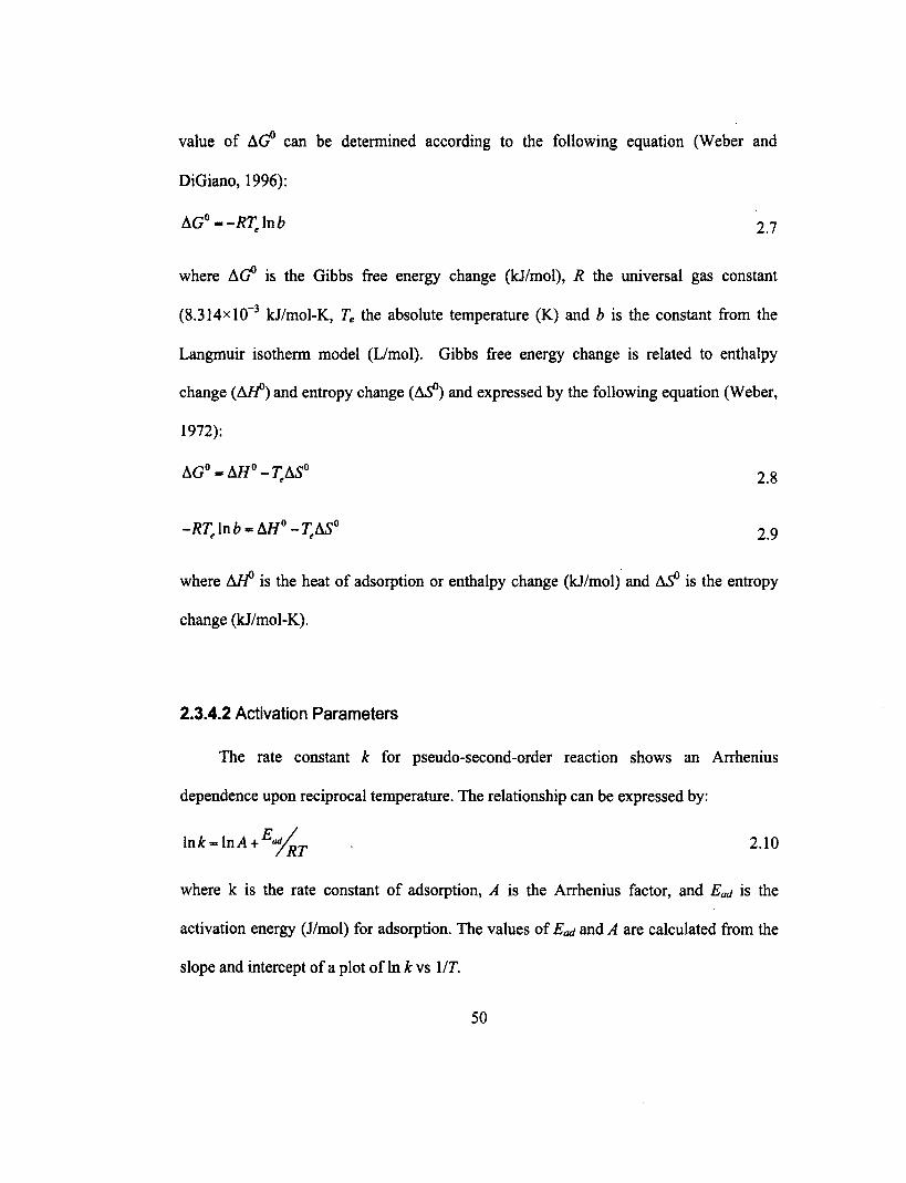
value of AG° can be determined according to the following equation (Weber and
DiGiano, 1996):
AG° -RT: In b 2.7
where AG° is the Gibbs free energy change (kJ/mol), R the universal gas constant
(8.314x 10⁻³ kJ/mol-K, Te the absolute temperature (K) and b is the constant from the
Langmuir isotherm model (L/mol). Gibbs free energy change is related to enthalpy
change (AH°) and entropy change (AS°) and expressed by the following equation (Weber,
1972):
AG° AH° - TAS° 2.8
-RT, In b MI° -TAS° 2.9
where AH° is the heat of adsorption or enthalpy change (kJ/mol) and AS° is the entropy
change (kJ/mol-K).
2.3.4.2 Activation Parameters
The rate constant k for pseudo-second-order reaction shows an Arrhenius
dependence upon reciprocal temperature. The relationship can be expressed by:
Ink-InA+Ea/ RT 2.10
where k is the rate constant of adsorption, A is the Arrhenius factor, and E ad is the
activation energy (J/mol) for adsorption. The values of E ad and A are calculated from the
slope and intercept of a plot of Ink vs 1/T.
50
value of AG0 can be determined according to the following equation (Weber and
DiGiano, 1996):
AG0 "-RT e \nb 2.7
where AG0 is the Gibbs free energy change (kJ/mol), R the universal gas constant
(8.314xl0-3 kJ/mol-K, Te the absolute temperature (K) and b is the constant from the
Langmuir isotherm model (L/mol). Gibbs free energy change is related to enthalpy
change (Aff) and entropy change (AS0) and expressed by the following equation (Weber,
1972):
&G°-AH°-T eM° 2.8
-RTe In = Aif0 - TeAS° 2.9
where A//0 is the heat of adsorption or enthalpy change (kJ/mol) and A5° is the entropy
change (kJ/mol-K).
2.3.4.2 Activation Parameters
The rate constant k for pseudo-second-order reaction shows an Arrhenius
dependence upon reciprocal temperature. The relationship can be expressed by:
lnfc = ln A + E°y^j 2.10
where k is the rate constant of adsorption, A is the Arrhenius factor, and Eaj is the
activation energy (J/mol) for adsorption. The values of Ead and A are calculated from the
slope and intercept of a plot of In k vs 1 IT.
50

2.3.5 Fixed Bed Column in Adsorption Studies
The successful design of a column adsorption process requires the prediction of the
concentration-time profile or breakthrough curve for the effluent. A number of
mathematical models have been developed to describe the concentration time profile in
order to assist in the design. In general, mechanisms operating in a biosorption column
involve axial dispersion in the direction of the liquid flow, film diffusion resistance, intra-
particle diffusion resistance which may include both pore and surface diffusion, and
sorption kinetics at the adsorbent surface (Chu 2004; Pagnanelli 2011). Non-linearity,
associated with equilibrium expressions, leads to sets of partial differential equations that
may require a complicated numerical solution. In addition, independent experiments may
be required to estimate the numerous equilibrium, transport, and sorption kinetic
parameters involved (Chu, 2004). Otherwise, multi-parameter fitting of breakthrough
curves may reduce the physical significance of the mechanistic parameters (Pagnanelli
2011). Obtaining a numerical solution with current computing facilities may no longer be
rigorous but semi-emperical or approximate methods are still extensively used to
simulate breakthrough curves of adsorption columns (Cooney 1999). Different kinetic
models, useful in process design, can be fitted to the column data to determine the
characteristic parameters of the column. Several widely used models for column design
are: Thomas, Yan, Belter, Chu, Yoon—Nelson, Oulman, and Wolborska models. The
Thomas model (Thomas 1948) is a second order reversible reaction model while Bohart—
Adams is a quasi-chemical kinetic model (Wang et al. 2010). The Yan model (Yan et al.
2001) is a dose—response model while the Belter and Cussler model (Belter and Cussler
51
2.3.5 Fixed Bed Column in Adsorption Studies
The successful design of a column adsorption process requires the prediction of the
concentration-time profile or breakthrough curve for the effluent. A number of
mathematical models have been developed to describe the concentration time profile in
order to assist in the design. In general, mechanisms operating in a biosorption column
involve axial dispersion in the direction of the liquid flow, film diffusion resistance, intra-
particle diffusion resistance which may include both pore and surface diffusion, and
sorption kinetics at the adsorbent surface (Chu 2004; Pagnanelli 2011). Non-linearity,
associated with equilibrium expressions, leads to sets of partial differential equations that
may require a complicated numerical solution. In addition, independent experiments may
be required to estimate the numerous equilibrium, transport, and sorption kinetic
parameters involved (Chu, 2004). Otherwise, multi-parameter fitting of breakthrough
curves may reduce the physical significance of the mechanistic parameters (Pagnanelli
2011). Obtaining a numerical solution with current computing facilities may no longer be
rigorous but semi-emperical or approximate methods are still extensively used to
simulate breakthrough curves of adsorption columns (Cooney 1999). Different kinetic
models, useful in process design, can be fitted to the column data to determine the
characteristic parameters of the column. Several widely used models for column design
are: Thomas, Yan, Belter, Chu, Yoon-Nelson, Oulman, and Wolborska models. The
Thomas model (Thomas 1948) is a second order reversible reaction model while Bohart-
Adams is a quasi-chemical kinetic model (Wang et al. 2010). The Yan model (Yan et al.
2001) is a dose-response model while the Belter and Cussler model (Belter and Cussler
51

1988) is a simple two-parameter model. The design criteria for lab scale packed bed
columns, as suggested in the literature, is given in Table 2.4 and the design details
regarding the lab scale packed columns, used in various biosorption studies, are provided
in Table 2.5. The design criteria, available in the literature, differ considerably.
Crittenden and Sowerby (1990) stated that conflicting criteria for packed bed
reactors arose when attempting to minimize the effects of radial temperature gradients
and channeling and wall effects. Carberry (1976) recommends a column to particle
diameter of less than 5 to 6 to avoid excessive radial temperature gradients. Whereas
Rase (1977) recommends the ratio should be greater than about 10 to avoid channeling
and wall effects (Crittenden and Sowerby 1990).
2.3.5.1 The Thomas Model
The Thomas model is widely used to evaluate column performance. It can be used
to predict a breakthrough curve and the maximum solute uptake by an adsorbent. The
Thomas model (Thomas 1948) has the following form (Reynolds and Richards 1996):
C0 1+ exp (K7/ Qfqom — Coll)
2.11
where Ce is the effluent adsorbate concentration (mg/L); Co the influent adsorbate
concentration (mg/L); KT the Thomas rate constant (L/min mg); qo the maximum solid
phase concentration of the solute (mg/g); m the mass of the adsorbent (g); V the
throughput volume (mL); and Q is the volumetric flow rate (mL/min).
52
1988) is a simple two-parameter model. The design criteria for lab scale packed bed
columns, as suggested in the literature, is given in Table 2.4 and the design details
regarding the lab scale packed columns, used in various biosorption studies, are provided
in Table 2.5. The design criteria, available in the literature, differ considerably.
Crittenden and Sowerby (1990) stated that conflicting criteria for packed bed
reactors arose when attempting to minimize the effects of radial temperature gradients
and channeling and wall effects. Carberry (1976) recommends a column to particle
diameter of less than 5 to 6 to avoid excessive radial temperature gradients. Whereas
Rase (1977) recommends the ratio should be greater than about 10 to avoid channeling
and wall effects (Crittenden and Sowerby 1990).
2.3.5.1 The Thomas Model
The Thomas model is widely used to evaluate column performance. It can be used
to predict a breakthrough curve and the maximum solute uptake by an adsorbent. The
Thomas model (Thomas 1948) has the following form (Reynolds and Richards 1996):
where Ce is the effluent adsorbate concentration (mg/L); C0 the influent adsorbate
concentration (mg/L); Kj the Thomas rate constant (L/min mg); q0 the maximum solid
phase concentration of the solute (mg/g); m the mass of the adsorbent (g); V the
throughput volume (mL); and Q is the volumetric flow rate (mL/min).
Q 2.11
52

Table 2.4: Design criteria for packed bed columns
Remarks Design criteria Reference
Lab columns, to Diameter of column — At least 4 in; Height Benefield et al. reduce wall effects of column -25-35 ft; Flow rate — Minimum (1982)
1 gpm/ft2; Diameter of column: particle diameter - 25:1; Empty bed contact time -20 to 50 min
Lab or pilot Diameter of column - Minimum 2.54 cm columns (1 in); Height of column - Minimum 61cm
(24 in)
Diameter of column - 3.5 cm; Flow rate - Reynolds and
Lab or pilot Maximum 0.5 gpm/ ft2 Richards (1995)
columns - To avoid channeling
Flow rate - Maximum 1 gpm/ft2
Diameter of column - 9.5 cm; Flow rate -Maximum 1.5 gpm/ft2
To investigate Flow rate - 1-3 gpm/ ft2; Recommended effects of flow rates
midrange flow rate - 0.5-4 gpm/ ft2
Perrich (1981) Typical values feasible for most applications
Empty bed contact time - 15, 30, 60, 90, 120 min
For GAC Empty bed contact time - 5-30 min Asano et al. contactors (2006)
Rapid small scale Diameter of column - 2-4 cm; height of Crittenden et al. column test column — 30 cm; length of bed - 5-15 cm; (1991)
Height of column: diameter of particle -20:1 (or greater)
For isothermal Turbulent conditions (Re>10); Height of operation column: diameter of column more than 20
Axial peclet number important
Height of column: particle diameter - Less than 50 Carberry (1976)
Avoid channeling Diameter of column: particle diameter -& wall effects Less than 5 to 6
Avoid channeling Diameter of column: particle diameter - Rase (1977) & wall effects Greater than about 10
Account column height: particle dia 100 or less Hill (1977) Dispersion
53
Table 2.4: Design criteria for packed bed columns
Remarks Design criteria Reference
Lab columns, to reduce wall effects
Lab or columns
pilot
Lab or pilot columns - To avoid channeling
To investigate effects of flow rates
Typical values feasible for most applications
For contactors
GAC
Rapid small scale column test
For isothermal operation
Axial peclet number important
Avoid channeling & wall effects
Avoid channeling & wall effects
Account Dispersion
Diameter of column - At least 4 in; Height of column -25-35 ft; Flow rate - Minimum 1 gpm/ft2; Diameter of column: particle diameter - 25:1; Empty bed contact time -20 to 50 min
Diameter of column - Minimum 2.54 cm (1 in); Height of column - Minimum 61cm (24 in)
Diameter of column - 3.5 cm; Flow rate -Maximum 0.5 gpm/ ft2
Flow rate - Maximum 1 gpm/ft2
Diameter of column - 9.5 cm; Flow rate -Maximum 1.5 gpm/ft2
Flow rate - 1-3 gpm/ ft2; Recommended midrange flow rate - 0.5-4 gpm/ ft2
Empty bed contact time - 15, 30, 60, 90, 120 min
Empty bed contact time - 5-30 min
Diameter of column - 2-4 cm; height of column - 30 cm; length of bed - 5-15 cm; Height of column: diameter of particle -20:1 (or greater)
Turbulent conditions (Re>10); Height of column: diameter of column more than 20
Height of column: particle diameter - Less than 50
Diameter of column: particle diameter -Less than 5 to 6
Diameter of column: particle diameter -Greater than about 10
column height: particle dia 100 or less
Benefield et al. (1982)
Reynolds and Richards (1995)
Perrich (1981)
Asano et al. (2006)
Crittenden et al. (1991)
Carberry (1976)
Rase (1977)
Hill (1977)
53

Table 2.5: Design details of lab scale columns used in biosorption studies
Dia of column (cm)
Length of bed (cm)
Flow rate (mL/ min)
Empty bed contact time (min)
Hydraulic loading rate (gpm/ft2)
Sorbent used/ material removed from water
Reference
3 10.3 0.58 A. niger/ Cd, Kapoor and
1.27 24.5 Cu, Pb Viraraghavan
1.8 17.2 0.35 A. niger/Ni (1998)
Fu and 1.27 23.5 6 4.9 1.16 A. niger! dyes Viraraghavan
(2003) 2.28 16.1 0.44 M rouxii/ Pb Yan and
1.27 29 2.59 2.66
14.2 13.8
0.50 0.52
M rouxii/ Cd M rouxii/Ni
Viraraghavan (2001)
2.22 16.5 0.43 M rouxii/ Zn
1.6 55 2.4 46.1 0.29 A. niger/ Cr Mungasavalliet al. (2007) Mathialagan
3.18 38 8 37.7 0.25 Perlite/ Cd andViraraghavan (2002)
1.25 20 12 2.0 2.40 Vermicul-ite! oil
Mysore et al. (2006)
Organoc-lay Moazed and 1.9 100 12 23.6 1.04 anthracite! oil Viraraghavan
(Breakthrough) (2001) 12 23.6 1.04
1.9 100
16 20 24 28
17.7 14.2 11.8 10.1
1.39 1.73 2.08 2.43
Organoclay- anthracite! oil (Breakdown)
Moazed and Viraraghavan (2002)
32 8.9 2.77
10 30 50 47.1 0.16 Peat/ oil (B reakthrough)
Mathavan and Viraraghavan (1989)
4.3 120.0 6.0 290.3 0.1 S. cerevisiae/ Ramirez et al. 12.0 145.1 0.2 Cr (III) and Cr (2007) 15.0 116.1 0.3 (VI)
54
Table 2.5: Design details of lab scale columns used in biosorption studies
Dia of column (cm)
Length of bed (cm)
Flow rate (mL/ min)
Empty bed contact time (min)
1.27 24.5 3
1.8
10.3
17.2
1.27 23.5 6 4.9
1.27 29
2.28 2.59 2.66 2.22
16.1 14.2 13.8 16.5
1.6 55 2.4 46.1
3.18 38 8 37.7
1.25 20 12 2.0
1.9 100 12 23.6
1.9 100
12 16 20 24 28 32
23.6 17.7 14.2 11.8 10.1 8.9
10 30 50 47.1
4.3 120.0 6.0 12.0 15.0
290.3 145.1 116.1
Hydraulic loading rate (gpm/ft2)
Sorbent used/ material removed from water
Reference
0.58
0.35
1.16
0.44 0.50 0.52 0.43
0.29
0.25
2.40
1.04
1.04 1.39 1.73 2.08 2.43 2.77
0.16
0.1 0.2 0.3
A. niger/ Cd, Cu, Pb
A. niger/ Ni
A. niger/ dyes
M. rouxii/ Pb M. rouxii/ Cd M. rouxii/ Ni M. rouxii/ Zn
A. niger/ Cr
Perlite/ Cd
Vermicul-ite/ oil Organoc-lay anthracite/ oil (Breakthrough)
Organoclay-anthracite/ oil (Breakdown)
Peat/ oil (Breakthrough)
S. cerevisiae/ Cr (III) and Cr (VI)
Kapoor and Viraraghavan (1998)
Fu and Viraraghavan (2003) Yan and Viraraghavan (2001)
Mungasavalli etal. (2007) Mathialagan and Viraraghavan (2002) Mysore et al. (2006) Moazed and Viraraghavan (2001)
Moazed and Viraraghavan (2002)
Mathavan and Viraraghavan (1989) Ramirez et al. (2007)
54

Table 2.5: Design details of lab scale columns used in biosorption studies (contd.)
Dia of column (cm)
Length of bed (cm)
Flow rate (mL/ min)
Empty bed contact time (min)
Hydraulic loading rate (gpm/ft)
Sorbent used/ material removed from water
Reference
1.0 30.0 0.5 47.1 0.2 Bottom ash and de-oiled soya/
Mittal et al. (2008)
Metanil Yellow
0.8 8.0 0.4 10.5 0.2 Cedar saw Hamdaoui (2006) 0.9 4.6 0.4 dust/ 2.0 2.0 1.0 Methylene
0.8 16.0 0.4 21.0 0.2 Blue 0.9 9.3 0.4 2.0 4.0 1.0
1.0 6.0 0.8 5.4 0.3 Immobilize Aksu and Gonen 1.6 2.7 0.5 d activated (2004) 3.2 1.4 1.1 sludge/
phenol 1.2 15.0 8.2 2.1 1.8 Natural Han et al. (2007a)
5.2 3.3 1.1 zeolite/ 2.2 7.7 0.5 Methylene
Blue 1.5 8.4 8.2 1.8 1.1 Rice husk/ Han et al. (2007b)
13.0 8.2 2.8 Methylene 25.4 8.2 5.5 Blue 39.0 8.2 8.4
2.8 30.6 6.0 31.4 0.2 Sargassum sp. / copper
Borba et al. (2008)
(II)
55
Table 2.5: Design details of lab scale columns used in biosorption studies (contd.)
Dia of Length Flow Empty Hydraulic Sorbent Reference column of bed rate bed loading used/ (cm) (cm) (mL/ contact rate material
min) time (gpm/ft2) removed (min) from water
1.0 30.0 0.5 47.1 0.2 Bottom ash Mittal et al. (2008) and de-oiled soya/ Metanil Yellow
0.8 8.0 0.4 10.5 0.2 Cedar saw Hamdaoui (2006) 0.9 4.6 0.4 dust/ 2.0 2.0 1.0 Methylene
0.8 16.0 0.4 21.0 0.2 Blue 0.9 9.3 0.4 2.0 4.0 1.0
1.0 6.0 0.8 5.4 0.3 Immobilize Aksu and Gonen 1.6 2.7 0.5 d activated (2004) 3.2 1.4 1.1 sludge/
phenol 1.2 15.0 8.2 2.1 1.8 Natural Han et al. (2007a)
5.2 3.3 1.1 zeolite/ 2.2 7.7 0.5 Methylene
Blue 1.5 8.4 8.2 1.8 1.1 Rice husk/ Han et al. (2007b)
13.0 8.2 2.8 Methylene 25.4 8.2 5.5 Blue 39.0 8.2 8.4
2.8 30.6 6.0 31.4 0.2 Sargassum Borba et al. (2008) sp. / copper (II)
55

The rate constant, KT, is a lumped parameter containing the effects of both intrinsic
kinetics and mass transfer. Its value is dependent upon the relative magnitudes of the
processes, which may be affected by the operating conditions and system variables of the
fixed bed column (Wang et al. 2010). The difference between breakthrough curves
calculated from the Thomas model and from other realistic diffusion equation models is
small (Ruthven, 1984).
2.3.5.2 The Yan Model
Column kinetics in a biosorption column was described by a modified dose—
response model proposed by Yan et al. (2001) and the Thomas model. The model was
developed for heavy metal removal in a biosorption column and is used to describe the
binary response regression problem. The logistic equation is expressed as follows:
Ce = 1
Co
1
1+{/} a
2.12
where d is the throughput volume that produces the same Ce/C0 value at 50% removal
and a is the constant, denoting the slope of the function.
2.3.5.3 The Belter and Chu Models
The models used in this study were the models developed by Belter et al. (1988)
(Equation 2.13) and modified by Chu (2004), as shown in Equations 2.14 and 2.15.
56
The rate constant, Kj, is a lumped parameter containing the effects of both intrinsic
kinetics and mass transfer. Its value is dependent upon the relative magnitudes of the
processes, which may be affected by the operating conditions and system variables of the
fixed bed column (Wang et al. 2010). The difference between breakthrough curves
calculated from the Thomas model and from other realistic diffusion equation models is
small (Ruthven, 1984).
2.3.5.2 The Yan Model
Column kinetics in a biosorption column was described by a modified dose-
response model proposed by Yan et al. (2001) and the Thomas model. The model was
developed for heavy metal removal in a biosorption column and is used to describe the
binary response regression problem. The logistic equation is expressed as follows:
where d is the throughput volume that produces the same CJCQ value at 50% removal
and a is the constant, denoting the slope of the function.
2.3.5.3 The Belter and Chu Models
The models used in this study were the models developed by Belter et al. (1988)
(Equation 2.13) and modified by Chu (2004), as shown in Equations 2.14 and 2.15.
2.12
56

t —t0_1i(i+erfCo y2ato
Ce 1 Co 2
Ce 1
Co 2
1+ erf
1+ erf
t—t0)exp(a(X0))
(t— t0)exp(—a(yto ))
Via;
2.13
2.14
2.15
where erf(x) is the error function of x, t the residence time inside the column, to the
temporal parameter which indicates the time required for the outlet contaminant
concentration to be half of the one inlet contaminant concentration and a is the standard
deviation which is a measure of the slope of the breakthrough curve. Model parameters to
and a can be estimated by fitting Equations 2.14 and 2.15 into the experimental
breakthrough data.
2.3.5.4 The Yoon and Nelson Model
Yoon and Nelson (1984) have developed a relatively simple model addressing
adsorption and breakthrough of adsorbate vapors or gases with respect to activated
charcoal. The Yoon and Nelson equation, related to a single- component system, is
expressed as:
57
£l Co
2.13
('-'•)rap(CT(X)) 2.14
(,-,„)exp (-a(^J) 2.15
where erf(x) is the error function of x, t the residence time inside the column, to the
temporal parameter which indicates the time required for the outlet contaminant
concentration to be half of the one inlet contaminant concentration and a is the standard
deviation which is a measure of the slope of the breakthrough curve. Model parameters to
and a can be estimated by fitting Equations 2.14 and 2.15 into the experimental
breakthrough data.
2.3.5.4 The Voori and Nelson Model
Yoon and Nelson (1984) have developed a relatively simple model addressing
adsorption and breakthrough of adsorbate vapors or gases with respect to activated
charcoal. The Yoon and Nelson equation, related to a single- component system, is
expressed as:
57

In t -t K Co - C
YN y 2 YN 2.16
where KYN is the rate constant (min-I); tut, the time required for 50% adsorbate
breakthrough (min) and t is the breakthrough time (min). Values of KYN and ti /2 may be
determined from a plot of in C/(Co-C) versus sampling time (t) according to Equation
2.16. If the theoretical model accurately characterizes the experimental data, this plot will
result in a straight line with slope of Km and an intercept KYN t1/2.
2.3.5.5 The Oulman Model
Oulman proposed the use of a bed depth service model to simulate Granular
Activated Carbon (GAC) adsorption beds (Oulman 1980). The model was first developed
by Bohart and Adams (1920) and based upon surface reaction theory. The Bohart-Adams
equation is as follows:
ln ...1).KNx
KC °t t 2.17
in which C is the effluent concentration (mg/L); Co is the influent concentration (mg/L);
K is the adsorption rate coefficient (L /mg min); N is the adsorption capacity coefficient
(mg/L); x is the bed depth (cm); u is the linear velocity (cm/min); and t is the time (min).
The Bohart-Adams equation can be rewritten as Equation 2.18 where a = KNxIu and b =
KC0.
C 1
C o 1+ e °-b`
58
2.18
2.16
where KYN is the rate constant (min-1); ti/2, the time required for 50% adsorbate
breakthrough (min) and t is the breakthrough time (min). Values of KYN and ti/2 may be
determined from a plot of In C/(Co-C) versus sampling time (t) according to Equation
2.16. If the theoretical model accurately characterizes the experimental data, this plot will
result in a straight line with slope of KYN and an intercept KYN ti/2.
2.3.5.5 The Oulman Model
Oulman proposed the use of a bed depth service model to simulate Granular
Activated Carbon (GAC) adsorption beds (Oulman 1980). The model was first developed
by Bohart and Adams (1920) and based upon surface reaction theory. The Bohart-Adams
equation is as follows:
in which C is the effluent concentration (mg/L); Co is the influent concentration (mg/L);
K is the adsorption rate coefficient (L /mg min); N is the adsorption capacity coefficient
(mg/L); x is the bed depth (cm); u is the linear velocity (cm/min); and t is the time (min).
The Bohart-Adams equation can be rewritten as Equation 2.18 where a = KNx/u and b =
2.17
KC0.
C 1
C0 " l + ea~b' 2.18
58

The Oulman model, as given by Equation 2.18 is equivalent to the 'logistic curve', an S-
shaped curve that is symmetrical around its midpoint at 1= a/b, C = C0/2.
2.3.5.6 The Wolborska Model
The Wolborska (1989) model generally describes the concentration distribution in
the bed for the low concentration region (low C/C0) of the breakthrough curve:
C Cot I 3 In C: a a
C 0 N 0 U 0
2.19
where pa is the kinetic coefficient of the external mass transfer (min-1), Na is the
saturation concentration in the Wolborska model (mg/L), Uo is the superficial velocity
(mm/min), and Z is the height of the column (mm). The expression of the Wolborska
model is equivalent to the Adams-Bohart model if coefficient k is equal to 13./N0. So, the
parameters in the two models can be determined from a plot of In (C/C0) against t at a
given bed height and flow rate.
2.4 Breakdown Mechanisms
2.4.1 Filtration Mechanisms
Particle removal mechanisms of granular media filtration may be divided into two
sequential steps: transport and attachment. Mechanisms involved in the transport of a
particle, from the bulk fluid to the surface of the filter medium, may include straining,
sedimentation, diffusion, interception, hydrodynamics, and flocculation. The mechanisms
59
The Oulman model, as given by Equation 2.18 is equivalent to the 'logistic curve', an S-
shaped curve that is symmetrical around its midpoint at t ~ alb, C = Co/2.
2.3.5.6 The Wolborska Model
The Wolborska (1989) model generally describes the concentration distribution in
the bed for the low concentration region (low C/Co) of the breakthrough curve:
I„£.ASL, M 219 c0 N, u„
where pa is the kinetic coefficient of the external mass transfer (min-1), N0 is the
saturation concentration in the Wolborska model (mg/L), U0 is the superficial velocity
(mm/min), and Z is the height of the column (mm). The expression of the Wolborska
model is equivalent to the Adams-Bohart model if coefficient k is equal to pa/iVo- So, the
parameters in the two models can be determined from a plot of In (C/Co) against t at a
given bed height and flow rate.
2.4 Breakdown Mechanisms
2.4.1 Filtration Mechanisms
Particle removal mechanisms of granular media filtration may be divided into two
sequential steps: transport and attachment. Mechanisms involved in the transport of a
particle, from the bulk fluid to the surface of the filter medium, may include straining,
sedimentation, diffusion, interception, hydrodynamics, and flocculation. The mechanisms
59

of particle attachment to filter media may occur via physical adsorption (electrostatic,
electrokinetic, and vander Waals forces), chemical adsorption (bonding and chemical
interaction), and biological growth. Sherony and Kintner (1971a,b) presented the
following filtration models to predict the head-loss across a filter bed involving single and
two-phase flows, respectively:
36LUyck, (1— 0 2API - (For single-phase flow)
cqgce32.20
36LUyck2 (1— e, )2 2.21 (For two-phase flow)
(.1;
2 where, AP1= pressure drop across the bed for single-phase flow [M/L ]; AP2 = pressure
2 drop across the bed for two-phase flow [MA, yc= dynamic viscosity of the continuous
phase [M/LT]; k1= Carman-Kozeny constant for single-phase flow (dimensionless); k2=
Carman-Kozeny constant for two-phase flow (dimensionless); gc = acceleration due to
gravity, 9.8 m/s2 [M/T2]; E = porosity of immobilized biomass bed in single-phase flow
(dimensionless); et = porosity of immobilized biomass bed in two-phase flow
(dimensionless); df = average diameter of immobilized biomass beads [L]; L = bed length
[L]; and U = superficial velocity [LIT]. The Carman-Kozeny constant (k1) is related to the
shape factor (k0) by the following equation (Carman 1956):
k,- koT2 2.22
where T is tortuosity. The value of T depends upon the pore structure of the medium.
With respect to pores of a medium having a straight path, the value of T is 1. As for a
medium having a non-straight path of pores, the value of T can be estimated as 1/e
60
of particle attachment to filter media may occur via physical adsorption (electrostatic,
electrokinetic, and vander Waals forces), chemical adsorption (bonding and chemical
interaction), and biological growth. Sherony and Kintner (1971a,b) presented the
following filtration models to predict the head-loss across a filter bed involving single and
two-phase flows, respectively:
. _ 36LUy ck.(l-£)2 2 20 AP, -—^—— (For single-phase flow)
d fg c£
A n 36LUy ck2{l-£,)2 ^ s 2.21 AP, —^ — (For two-phase flow)
df8A
2 where, APi= pressure drop across the bed for single-phase flow [M/L ]; AP2 = pressure
2 drop across the bed for two-phase flow [M/L ]; yc= dynamic viscosity of the continuous
phase [M/LT]; ki= Carman-Kozeny constant for single-phase flow (dimensionless); k2=
Carman-Kozeny constant for two-phase flow (dimensionless); gc = acceleration due to
2 , gravity, 9.8 m/s [M/T ]; e = porosity of immobilized biomass bed in single-phase flow
(dimensionless); et = porosity of immobilized biomass bed in two-phase flow
(dimensionless); df = average diameter of immobilized biomass beads [L]; L = bed length
[L]; and U = superficial velocity [L/T], The Carman-Kozeny constant (ki) is related to the
shape factor (ko) by the following equation (Carman 1956):
*1 - KT1 2.22
where T is tortuosity. The value of T depends upon the pore structure of the medium.
With respect to pores of a medium having a straight path, the value of T is 1. As for a
medium having a non-straight path of pores, the value of T can be estimated as 1/e
60

(Johnston 1983).
One very important concept in applying filtration equations to two-phase flow is
that of relative permeability. Bear (1972) outlined factors affecting relative permeability
and stated saturation had a considerable effect upon the other parameters. The specific
permeability coefficient (Bo) of materials having high porosities can be calculated using
the following relationship, as proposed by Kozeny (Carman 1956):
d2E32.23 Bo -
16k1 (1 —
The Kozeny equation for a specific permeability coefficient is applicable to laminar
flows. According to Sherony et al. (1978), the condition for laminar flow is:
NRe <10 (1—e)
where NRe is the Reynolds number.
2.24
2.4.2 Coalescence Mechanisms
The coalescence process can be described as a phenomenon in which droplets
from the discontinuous phase of an emulsion tend to produce extensively large droplets
until eventually a separate phase may be created (Schramm 1992). The process is usually
initiated by a collision between the droplets that is sufficient enough to break the
interfacial film. Once the droplets are in physical contact, the process is completed by
surface forces (Chieu et al. 1975). The coalescence mechanism takes place according to
three major steps (Hazlett 1969): approach, attachment, and release. The approach
61
(Johnston 1983).
One very important concept in applying filtration equations to two-phase flow is
that of relative permeability. Bear (1972) outlined factors affecting relative permeability
and stated saturation had a considerable effect upon the other parameters. The specific
permeability coefficient (Bo) of materials having high porosities can be calculated using
the following relationship, as proposed by Kozeny (Carman 1956):
B - ^ 2.23 ° 16^(1-e)2
The Kozeny equation for a specific permeability coefficient is applicable to laminar
flows. According to Sherony et al. (1978), the condition for laminar flow is:
7^ <10 2.24 (l-e)
where Afa is the Reynolds number.
2.4.2 Coalescence Mechanisms
The coalescence process can be described as a phenomenon in which droplets
from the discontinuous phase of an emulsion tend to produce extensively large droplets
until eventually a separate phase may be created (Schramm 1992). The process is usually
initiated by a collision between the droplets that is sufficient enough to break the
interfacial film. Once the droplets are in physical contact, the process is completed by
surface forces (Chieu et al. 1975). The coalescence mechanism takes place according to
three major steps (Hazlett 1969): approach, attachment, and release. The approach
61
mechanism involves bringing a dispersed-phase droplet to the surface of the filter
medium or to the surface of a droplet attached to the surface medium. The main forces
involved in the approach step include interception, diffusion, inertial impaction,
electrostatic attraction, van der Waals force and sedimentation (Hazlett 1969). In the
attachment process, the oil droplets displace water film from the surface of the material
and preferentially wet its surface. If the media is wetted by the dispersed phase, drops
will coalescence onto the media surface to form a film upon which subsequent drops will
coalesce. However, if the media is not wetted by the dispersed phase, coalescence
between drops will occur in the pores of the media. In the release step, the hydrodynamic
force acting upon a drop overcomes the adhesive force between the droplet and the
material (Hazlett 1969). Several mathematical models have been developed to describe
the process of coalescence. Sheroney and Kintner (1971 a,b) developed a collision model,
which relates the overall collision frequency between droplets and particles of the bed to
the overall coalescence efficiency. The theory of the model was based largely upon the
impaction contact mechanism: droplets moving with the continuous phase collide with
other droplets previously attached to the medium. Although other mechanisms were
identified, it was shown that the order of magnitude of collision frequencies due to
impaction was high enough to neglect the other mechanisms (Sheroney and Kintner,
1971a). This model predicts the ratio of outlet to inlet particle number densities (Y) in
terms of other parameters as follows:
62
mechanism involves bringing a dispersed-phase droplet to the surface of the filter
medium or to the surface of a droplet attached to the surface medium. The main forces
involved in the approach step include interception, diffusion, inertial impaction,
electrostatic attraction, van der Waals force and sedimentation (Hazlett 1969). In the
attachment process, the oil droplets displace water film from the surface of the material
and preferentially wet its surface. If the media is wetted by the dispersed phase, drops
will coalescence onto the media surface to form a film upon which subsequent drops will
coalesce. However, if the media is not wetted by the dispersed phase, coalescence
between drops will occur in the pores of the media. In the release step, the hydrodynamic
force acting upon a drop overcomes the adhesive force between the droplet and the
material (Hazlett 1969). Several mathematical models have been developed to describe
the process of coalescence. Sheroney and Kintner (1971a,b) developed a collision model,
which relates the overall collision frequency between droplets and particles of the bed to
the overall coalescence efficiency. The theory of the model was based largely upon the
impaction contact mechanism: droplets moving with the continuous phase collide with
other droplets previously attached to the medium. Although other mechanisms were
identified, it was shown that the order of magnitude of collision frequencies due to
impaction was high enough to neglect the other mechanisms (Sheroney and Kintner,
1971a). This model predicts the ratio of outlet to inlet particle number densities (Y) in
terms of other parameters as follows:
62

2.25
Y — exp 4 (1 —S,) d
where: c = porosity of the immobilized biomass beads (dimensionless); Sd = average
saturation (the fraction of the void volume occupied by the dispersed phase adhering to
the solid, dimensionless); di = average particle size of the distribution [L]; df =
immobilized biomass bead diameter; ic = the overall coalescence efficiency (fraction);
and L = bed length [L]. The Sherony and Kintner model was recently modified by Li and
Gu (2005), taking into consideration both the collisions between a droplet in the stream
and a droplet deposited on the solid surface and the collisions between two droplets in the
stream. However, this modified model has undergone only limited-testing and the
specific mechanisms affecting the overall coalescence efficiency of the granular beds
could not be adequately assessed.
If, Sd, di, df, E, L and Y are known, Tic can be determined using the above equation.
The values of di, df, c, L and Y can be measured experimentally. The assumptions based
upon which the above model was developed are (Sherony and Kintner 1971a,b): 1) the
model is confined to emulsion concentrations of 1000 mg/L or less flowing into the bed;
2) the bed is randomly packed fiber with a resident population of adhering drops and size
distribution of the held drops is constant with time; 3) the particles from the liquid
interact with the hold-up by collision; 4) the velocity is independent of particle mass; 5)
in the velocity region of interest, the impaction mechanism is predominant; 6) the number
density of particles to the fiber is dependent upon the degree of saturation of the bed; 7)
63
where: e = porosity of the immobilized biomass beads (dimensionless); Sa = average
saturation (the fraction of the void volume occupied by the dispersed phase adhering to
the solid, dimensionless); di = average particle size of the distribution [L]; df =
immobilized biomass bead diameter; r|c = the overall coalescence efficiency (fraction);
and L = bed length [L]. The Sherony and Kintner model was recently modified by Li and
Gu (2005), taking into consideration both the collisions between a droplet in the stream
and a droplet deposited on the solid surface and the collisions between two droplets in the
stream. However, this modified model has undergone only limited-testing and the
specific mechanisms affecting the overall coalescence efficiency of the granular beds
could not be adequately assessed.
If, Sd, di, df, E, L and Y are known, r|c can be determined using the above equation.
The values of dj, df, e, L and Y can be measured experimentally. The assumptions based
upon which the above model was developed are (Sherony and Kintner 1971a,b): 1) the
model is confined to emulsion concentrations of 1000 mg/L or less flowing into the bed;
2) the bed is randomly packed fiber with a resident population of adhering drops and size
distribution of the held drops is constant with time; 3) the particles from the liquid
interact with the hold-up by collision; 4) the velocity is independent of particle mass; 5)
in the velocity region of interest, the impaction mechanism is predominant; 6) the number
density of particles to the fiber is dependent upon the degree of saturation of the bed; 7)

emulsion flowing through the bed does not form a continuum; and 8) the possibility of a
collision between two drops is independent of drop diameter.
The average saturation (Sd) of the dispersed phase is related to the change in
porosity (et) by:
sd = (1 — ft) 2.26
The porosity of the bed in two-phase flow will be calculated using the following
relationship developed by dividing Equation 2.20 by Equation 2.21 and re-arranging:
dPik2e3 )3
'3—
AP2k, (1— e)2 (1 — e ,)22.27
where f3 is a dimensionless parameter.
The average saturation (Sd) in Equation 2.26 can be calculated using Equation
2.27. The average holdup is defined as the volume of dispersed phase per volume of solid
retained. The average holdup O H) of a bed can be calculated by the following equation,
as presented by Sherony et al. (1978):
Sd (1— e)
£
2.28
Breaking of naphtha/water and water/naphtha emulsions with a packed bed coalescence,
using Ottawa sand, was examined by Crickmore et al. (1989). Process variables
influencing the packed bed in coalescing emulsions were screened and the qualitative
relationship between the influential process variables and emulsion coalescence were
determined. The flow rate was identified as affecting the emulsion coalescence and other
variables such as the type of packing, packing size range, and temperature and was found
64
emulsion flowing through the bed does not form a continuum; and 8) the possibility of a
collision between two drops is independent of drop diameter.
The average saturation (S<j) of the dispersed phase is related to the change in
porosity (et) by:
The porosity of the bed in two-phase flow will be calculated using the following
relationship developed by dividing Equation 2.20 by Equation 2.21 and re-arranging:
where P is a dimensionless parameter.
The average saturation (Sd) in Equation 2.26 can be calculated using Equation
2.27. The average holdup is defined as the volume of dispersed phase per volume of solid
retained. The average holdup (0h) of a bed can be calculated by the following equation,
as presented by Sherony et al. (1978):
Breaking of naphtha/water and water/naphtha emulsions with a packed bed coalescence,
using Ottawa sand, was examined by Crickmore et al. (1989). Process variables
influencing the packed bed in coalescing emulsions were screened and the qualitative
relationship between the influential process variables and emulsion coalescence were
determined. The flow rate was identified as affecting the emulsion coalescence and other
variables such as the type of packing, packing size range, and temperature and was found
2.26
WAP"*)' "(l-e,)! "P
APfe3 E> 2.27
64

to have no significant effect. Preliminary examination revealed that coalescence of an
emulsion was solely a function of the residence time in the bed and a kinetic expression
should be able to correlate the coalescence data. The relationship between emulsion
coalescence and residence time was described by a first-order rate equation:
CA ws CA0 exp(-01 2.29
where, CA = fraction of fluid emulsified at t', CA0 = fraction of fluid emulsified at
entrance to the packed bed, IQ = rate constant for coalescence, t'= modified residence
time.
r
AE 2.30
where, t= residence time, A = cross-sectional area of the empty tube, and E = void
fraction of the packed bed.
65
to have no significant effect. Preliminary examination revealed that coalescence of an
emulsion was solely a function of the residence time in the bed and a kinetic expression
should be able to correlate the coalescence data. The relationship between emulsion
coalescence and residence time was described by a first-order rate equation:
C>CAoexp(-*cT') 2 29
where, CA = fraction of fluid emulsified at x', CA0 = fraction of fluid emulsified at
entrance to the packed bed, kc = rate constant for coalescence, x - modified residence
time.
T'-— 2.30 Ae
where, x= residence time, A = cross-sectional area of the empty tube, and e = void
fraction of the packed bed.
65

Chapter 3
Materials and Methods
3.1 Glassware Preparation
All glassware for use in the experiments was washed with a laboratory detergent,
rinsed with tap water, further washed with hydrochloric acid, and finally rinsed twice
with deionized water and dried prior to use.
3.2 Experimental Materials
Two fungal strains, Mucor rouxii and Absidia coerulea, were purchased from
American Type Culture Collection (ATCC), Rockville, Maryland, USA (ATCC #24905,
ATCC #10738a). Chitosan from crab shells (Aldrich 417963) was purchased from
Sigma-Aldrich Corporation, Ontario, Canada. Walnut shell media was supplied by
USFilter, part of the Water Technology division of Siemen's Industrial Solutions and
Services (I&S) Group, USA. Types of oil found in contaminated water include fats;
lubricants; cutting fluids; heavy hydrocarbons such as tars, grease, crude oil, diesel oils;
and light hydrocarbons such as kerosene, jet fuel, and gasoline (Braden, 1994). The
following oils were used in the study typically representing a refined mineral oil, a
vegetable oil and a cutting oil:
• Standard (light) Mineral Oil (SMO) marketed by Fisher Scientific Company,
USA, emulsified with oleic acid and triethanolamine using Regina tap water
according to the procedure used by Biswas (1973);
66

• Vegetable oil, Canola Oil (CO) marketed in Canada, emulsified in the same
manner as SMO; and
• DoALL Bright-Edge 80, a cutting oil manufactured by DoALL Company, IL,
USA, emulsified in the same manner as SMO;
3.3 Preparation of Oil-in-water Emulsions
Oil (21.25 g) was poured into a beaker to which 18.80 g of oleic acid was added.
This mixture was stirred continuously using a magnetic stirrer for 15 minutes, producing
a clear mixture followed by an addition of 9.95 g of triethanolamine. The resulting
mixture was stirred at a high speed to produce a clear mixture with bubbles inside the
solution. The oil mixture was diluted with tap water to two litres. This was then mixed
thoroughly in a blender for 15 minutes. This oil emulsion was used as a 25,000 mg/L
concentrate. The working stock solution was prepared by diluting with tap water. This oil
emulsion was prepared based on the procedure adopted by Biswas (1973).
3.4 Characterization of Oil-in-water Emulsions
The density of oils was determined by weighing a known volume (25 mL) of oil
in a pycnometer. Viscosity was measured according to ASTM (1963). The viscosity of
the oils was determined by comparing the efflux time of a liquid having a known
viscosity to that of oil with unknown viscosity, as given below:
67

12= WI/ P2t2 3.1
Where, t = Efflux time; p = Density of the liquid; rl 1 = Viscosity of water; and rl 2 =
Viscosity of oil. Interfacial tension of the oil was measured with a Spinning Drop
Interfacial Tensiometer Model 510 marketed by Temco Inc., Tulsa, Oklahoma, USA. The
surface charges of SMO and CO were taken from measurements done by Mysore et al.
(2005). Surface charge of Bright-Edge 80 cutting oil was measured using Zetasizer,
model HSA 3000 (Malvern, Worcestershire, England).
3.5 Preparation of Fungal Seed
Freeze dried cultures received from ATCC were activated in sterile water for
seeding. Deionized water (100 mL) was autoclaved for 15 minutes at 121 °C and 124 kPa
and allowed to cool to room temperature. Freeze dried cultures were soaked in 10 mL of
sterile water for 45 minutes before transferring to a potato-dextrose agar surface. Bacto
potato dextrose agar (PDA) 39 g/L was used to prepare the agar surfaces. Approximately
2 mL of this suspension was transferred to each PDA plate. The plates were incubated for
7-10 days at 22±2°C to fully activate the fungal strain. This culture was used to grow the
biomass for experimental purposes.
3.6 Preparation of Non-viable Fungal Biomass
M rouxii strain was routinely maintained on potato dextrose agar plates. It was
grown aerobically by the shake flask method. It was cultivated using a growth medium
68
til/ 112= pit]/ p2t2 3 i
Where, t = Efflux time; p = Density of the liquid; TI i = Viscosity of water; and t] 2 =
Viscosity of oil. Interfacial tension of the oil was measured with a Spinning Drop
Interfacial Tensiometer Model 510 marketed by Temco Inc., Tulsa, Oklahoma, USA. The
surface charges of SMO and CO were taken from measurements done by Mysore et al.
(2005). Surface charge of Bright-Edge 80 cutting oil was measured using Zetasizer,
model HSA 3000 (Malvern, Worcestershire, England).
3.5 Preparation of Fungal Seed
Freeze dried cultures received from ATCC were activated in sterile water for
seeding. Deionized water (100 mL) was autoclaved for 15 minutes at 121 °C and 124 kPa
and allowed to cool to room temperature. Freeze dried cultures were soaked in 10 mL of
sterile water for 45 minutes before transferring to a potato-dextrose agar surface. Bacto®
potato dextrose agar (PDA) 39 g/L was used to prepare the agar surfaces. Approximately
2 mL of this suspension was transferred to each PDA plate. The plates were incubated for
7-10 days at 22±2°C to fully activate the fungal strain. This culture was used to grow the
biomass for experimental purposes.
3.6 Preparation of Non-viabie Fungal Biomass
M. rouxii strain was routinely maintained on potato dextrose agar plates. It was
grown aerobically by the shake flask method. It was cultivated using a growth medium
68

comprised of yeast extract (3 g/L), peptone (10 g/L) and glucose (replaced by dextrose)
(20 g/L) (Bartnickni-Garcia and Nickerson 1962; Muzzarelli et al. 1994). The pH of the
growth medium was maintained at 4.5 by 1.0 N HCI. The culture was grown in an
aerobic condition at room temperature (22 ± 2°C) with 100 mL of the liquid medium in
250 mL conical flasks on a rotary shaker agitated at 125 rpm. M rouxii was harvested
after three days of growth by filtering the growth medium through a 150 gm sieve. The
harvested fungal biomass was washed with generous amounts of deionized water and
autoclaved for 30 minutes at 121°C and 103 kPa. The autoclaved biomass was allowed to
cool and dried in an oven at 60 °C for 24 hours. The dried biomass was powdered into a
fine size using a grinder. The biomass passing through a 400 mesh sieve was used for the
experiment. A. coerulea strains were also prepared in the same manner as those of M
rouxii, except that the pH of the growth medium for A. coerulea was maintained at 5.0 by
1.0 N HCI and was harvested after 4 days of growth.
3.7 Characterization of Fungal Biomass
Porosity of the adsorbent was determined by the graduated cylinder technique
(AEEP 1988) by placing a known volume of adsorbent into a measuring cylinder and
filling it with water. The amount of water required to fill in the voids was measured and
the porosity determined. The moisture content of the adsorbent was measured by
electronic balance according to ASTM (1992). The samples were mixed thoroughly and a
known amount was placed in the pre-weighed porcelain dish. The sample was then oven-
dried at 105°C for 16 hours, cooled and weighed. The loss in weight was used to
69
comprised of yeast extract (3 g/L), peptone (10 g/L) and glucose (replaced by dextrose)
(20 g/L) (Bartnickni-Garcia and Nickerson 1962; Muzzarelli et al. 1994). The pH of the
growth medium was maintained at 4.5 by 1.0 N HC1. The culture was grown in an
aerobic condition at room temperature (22 ± 2°C) with 100 mL of the liquid medium in
250 mL conical flasks on a rotary shaker agitated at 125 rpm. M. rouxii was harvested
after three days of growth by filtering the growth medium through a 150 |im sieve. The
harvested fungal biomass was washed with generous amounts of deionized water and
autoclaved for 30 minutes at 121 °C and 103 kPa. The autoclaved biomass was allowed to
cool and dried in an oven at 60 °C for 24 hours. The dried biomass was powdered into a
fine size using a grinder. The biomass passing through a 400 mesh sieve was used for the
experiment. A. coerulea strains were also prepared in the same manner as those of M.
rouxii, except that the pH of the growth medium for A coerulea was maintained at 5.0 by
1.0 N HCI and was harvested after 4 days of growth.
3.7 Characterization of Fungal Biomass
Porosity of the adsorbent was determined by the graduated cylinder technique
(AEEP 1988) by placing a known volume of adsorbent into a measuring cylinder and
filling it with water. The amount of water required to fill in the voids was measured and
the porosity determined. The moisture content of the adsorbent was measured by
electronic balance according to ASTM (1992). The samples were mixed thoroughly and a
known amount was placed in the pre-weighed porcelain dish. The sample was then oven-
dried at 105°C for 16 hours, cooled and weighed. The loss in weight was used to

calculate the moisture content. The pH of the adsorbent was determined by electronic
ASTM measurements (ASTM 1989). A known weight of the adsorbent was placed in 350
mL deionized water and allowed to soak for 30 minutes with occasional stirring. The pH
was then determined using an Accumet pH meter (Fisher Scientific Ltd, Model 600).
3.7.1 Surface Area Analysis and Surface Charge Measurement
Surface area and pore size measurements of the powdered autoclaved biomass
were carried out using Micromeritics® ASAP 2020 accelerated surface area and
porosimetry analyzer. The surface charge of the autoclaved M rouxii biomass was
measured using Zetasizer, model HSA 3000 (Malvern, Worcestershire, England) at the
University of Alberta, Canada. An average particle size of the biomass was also
measured using the Zetasizer.
3.7.2 Scanning Electron Microscope (SEM) Studies
Scanning Electron Microscope (SEM) images of biomass samples (before and after
sorption of oil) were obtained using a LEO FESEM 1530 unit with a field emission
Gemini Column. The samples were gold coated for 120 s prior to SEM scanning.
70
calculate the moisture content. The pH of the adsorbent was determined by electronic
ASTM measurements (ASTM 1989). A known weight of the adsorbent was placed in 350
mL deionized water and allowed to soak for 30 minutes with occasional stirring. The pH
was then determined using an Accumet pH meter (Fisher Scientific Ltd, Model 600).
3.7.1 Surface Area Analysis and Surface Charge Measurement
Surface area and pore size measurements of the powdered autoclaved biomass
were carried out using Micromeritics® ASAP 2020 accelerated surface area and
porosimetry analyzer. The surface charge of the autoclaved M. rouxii biomass was
measured using Zetasizer, model HSA 3000 (Malvern, Worcestershire, England) at the
University of Alberta, Canada. An average particle size of the biomass was also
measured using the Zetasizer.
3.7.2 Scanning Electron Microscope (SEM) Studies
Scanning Electron Microscope (SEM) images of biomass samples (before and after
sorption of oil) were obtained using a LEO FESEM 1530 unit with a field emission
Gemini Column. The samples were gold coated for 120 s prior to SEM scanning.
70

3.7.3 Fourier Transform Infrared (FTIR) Analysis
Autoclaved biomass and oil-loaded biomass were analyzed qualitatively on a Bio-
Rad FTS-60 infrared system using the potassium bromide (KBr) pellet technique (6 mg
sample/400 mg KBr).
3.8 Oil Concentration Measurement
Oil and grease are defined as any material recovered as a substance soluble in the
solvent (Franson and Eaton 2005). In the determination of oil and grease, an absolute
quantity of a specific substance is not measured; instead oil and grease are defined by the
method used for their determination (Franson and Eaton 2005). Although a variety of
non-hydrocarbon solvents are commercially available for the determination of oil and
grease using the Infrared (IR) method, for certain regulatory purposes, USEPA currently
recommends only n-hexane (Pushkarev et al. 1983; Franson and Eaton 2005; Tyrie and
Caudle 2007). As for liquid samples, the 21s` edition of Standard Methods prescribes four
methods for oil and grease determination: 1) the liquid/liquid partition-gravimetric
(5520B); 2) the partition-infrared (5520C); 3) the soxhelet method (5520D); and 4) the
solid-phase, partition-gravimetric (Franson and Eaton 2005). Several oil measurement
techniques such as gravimetric, IR, UltraViolet (UV) and colorimetric methods are listed
in Table 3.1. In the partition-gravimetric method (5520B), dissolved or emulsified oil is
extracted from water by intimate contact with an extracting solvent. However, this
method is not suitable for samples that contain volatile hydrocarbons, because they would
be lost in the solvent-removal operations of this procedure. Soxhlet method (5520D) is
71
3.7.3 Fourier Transform Infrared (FTIR) Analysis
Autoclaved biomass and oil-loaded biomass were analyzed qualitatively on a Bio-
Rad FTS-60 infrared system using the potassium bromide (KBr) pellet technique (6 mg
sample/400 mg KBr).
3.8 Oil Concentration Measurement
Oil and grease are defined as any material recovered as a substance soluble in the
solvent (Franson and Eaton 2005). In the determination of oil and grease, an absolute
quantity of a specific substance is not measured; instead oil and grease are defined by the
method used for their determination (Franson and Eaton 2005). Although a variety of
non-hydrocarbon solvents are commercially available for the determination of oil and
grease using the Infrared (IR) method, for certain regulatory purposes, USEPA currently
recommends only n-hexane (Pushkarev et al. 1983; Franson and Eaton 2005; Tyrie and
Caudle 2007). As for liquid samples, the 21st edition of Standard Methods prescribes four
methods for oil and grease determination: 1) the liquid/liquid partition-gravimetric
(5520B); 2) the partition-infrared (5520C); 3) the soxhelet method (5520D); and 4) the
solid-phase, partition-gravimetric (Franson and Eaton 2005). Several oil measurement
techniques such as gravimetric, IR, Ultraviolet (UV) and colorimetric methods are listed
in Table 3.1. In the partition-gravimetric method (5520B), dissolved or emulsified oil is
extracted from water by intimate contact with an extracting solvent. However, this
method is not suitable for samples that contain volatile hydrocarbons, because they would
be lost in the solvent-removal operations of this procedure. Soxhlet method (5520D) is
71

Table 3.1: Oil in water measurement methods
Method Extraction solvent Remarks Reference Gravimetric n-hexane Legally defines oil in the US. Franson and (USEPA Method 1664;
Measures only organic compounds that are extractable from water in n-hexane at pH
Eaton (2005)
Standard Methods
2.0 and that remain after hexane is evaporated.
5520B)
Infrared Trichlorotrifluro- C-H bond present in the oil Franson and (Standard ethane, non- absorbs IR energy at a Eaton (2005); Methods hydrocarbon wavelength of 3.41 µ (2900 cm" Tyrie and 5520C) solvents such as 1). Since water absorbs IR Caudle
tetrachlorothylene, carbon
energy at this wavelength, measurements must be made on
(2007); Ibrahim et al.
tetrachloride. a sample using a solvent that does not absorb IR radiation. Calibrated with a standard sample of known concentration.
(2009); Sokolovic et al. (2010)
Ultra violet Extraction solvents Aromatic compounds absorb UV Bastow et al. method such as isopropanol radiation and fluoresce. UV is (1997); Tyrie
have been reported. Measurements can also be made without an extraction solvent.
not absorbed by water. However, other components in the wastewater such as iron may fluoresce. So instruments using extraction have an advantage.
and Caudle (2007)
Colorimetric Generally no The absorption of energy in the Biswas methods extraction is visible light range is used as the (1973);
required. A solvent detection process. The Tellez et al. like methylene chloride has been used to impart color to the oil containing wastewater.
instrument needs to be calibrated with a known concentration.
(2005)
Particle No extraction is No calibration is required. Tyrie and counting required Particle counting methods
cannot normally see below 2 µ.. Caudle (2007)
72
Table 3.1: Oil in water measurement methods
Method Extraction solvent Remarks Reference Gravimetric (USEPA Method 1664; Standard Methods 5520B)
Infrared (Standard Methods 5520C)
n-hexane
Ultra violet method
Colorimetric methods
Particle counting
Trichlorotrifluro-ethane, non-hydrocarbon solvents such as tetrachlorothylene, carbon tetrachloride.
Extraction solvents such as isopropanol have been reported. Measurements can also be made without an extraction solvent.
Generally no extraction is required. A solvent like methylene chloride has been used to impart color to the oil containing wastewater.
No extraction is required
Legally defines oil in the US. Measures only organic compounds that are extractable from water in n-hexane at pH 2.0 and that remain after hexane is evaporated.
C-H bond present in the oil absorbs IR energy at a wavelength of 3.41 n (2900 cm" '). Since water absorbs IR energy at this wavelength, measurements must be made on a sample using a solvent that does not absorb IR radiation. Calibrated with a standard sample of known concentration.
Aromatic compounds absorb UV radiation and fluoresce. UV is not absorbed by water. However, other components in the wastewater such as iron may fluoresce. So instruments using extraction have an advantage.
The absorption of energy in the visible light range is used as the detection process. The instrument needs to be calibrated with a known concentration.
No calibration is required. Particle counting methods cannot normally see below 2 it.
Franson and Eaton (2005)
Franson and Eaton (2005); Tyrie and Caudle (2007); Ibrahim et al. (2009); Sokolovic et al. (2010)
Bastow et al. (1997); Tyrie and Caudle (2007)
Biswas (1973); Tellez et al. (2005)
Tyrie and Caudle (2007)
72

the method of choice when relatively polar, heavy petroleum fractions are present, or
when the levels of the nonvolatile greases may challenge the solubility limit of the
solvent. The infrared spectroscopic method may have an advantage over other methods
when determining the sum of extractables of unknown origin for which it is generally
difficult to plot a calibration curve. This is possible due to the fact that light absorption
bands of the C-H bond belong to the infrared region at a wavelength of 2900 aril . The C-
H bonds are mostly characteristic of any organic compound and the number of bonds per
unit of mass varies less for substances of variable composition than does the number of
any other functional group. Therefore, the calibration curves plotted for various types of
oils diverge by not more than 5 — 10% (Pushkarev et al. 1983). However, the infrared
absorption bands of water (0-H) bonds are also localized in the region around 3000 cm I.
Hence, the method requires complete elimination of water from the sample for which an
extracting solvent containing no C-H bonds should be used.
Due to its advantages and precision, the partition-infrared method was used in this
study. The use of IR techniques to measure oil in water has been widely reported in the
literature (Mathavan and Viraraghavan 1992; Moazed and Viraraghavan 2005; Mysore et
al. 2005). Other than conventional IR spectroscopy (Sokolovic 2010), equipment such as
Horiba OCMA 220, and InfraCal CVH have been reported to provide an analysis of oil
content of water samples (Mathavan and Viraraghavan 1992; Moazed and Viraraghavan
2005; Mysore et al. 2005; Ibrahim et al. 2009). Among IR techniques, oil determination
by Horiba OCMA 220 using different solvents has been extensively studied (Mathavan
and Viraraghavan 1990). Different solvents such as carbon tetrachloride and
73
the method of choice when relatively polar, heavy petroleum fractions are present, or
when the levels of the nonvolatile greases may challenge the solubility limit of the
solvent. The infrared spectroscopic method may have an advantage over other methods
when determining the sum of extractables of unknown origin for which it is generally
difficult to plot a calibration curve. This is possible due to the fact that light absorption
bands of the C-H bond belong to the infrared region at a wavelength of 2900 cm*1. The C-
H bonds are mostly characteristic of any organic compound and the number of bonds per
unit of mass varies less for substances of variable composition than does the number of
any other functional group. Therefore, the calibration curves plotted for various types of
oils diverge by not more than 5 - 10% (Pushkarev et al. 1983). However, the infrared
absorption bands of water (O-H) bonds are also localized in the region around 3000 cm"1.
Hence, the method requires complete elimination of water from the sample for which an
extracting solvent containing no C-H bonds should be used.
Due to its advantages and precision, the partition-infrared method was used in this
study. The use of IR techniques to measure oil in water has been widely reported in the
literature (Mathavan and Viraraghavan 1992; Moazed and Viraraghavan 2005; Mysore et
al. 2005). Other than conventional IR spectroscopy (Sokolovic 2010), equipment such as
Horiba OCMA 220, and InfraCal CVH have been reported to provide an analysis of oil
content of water samples (Mathavan and Viraraghavan 1992; Moazed and Viraraghavan
2005; Mysore et al. 2005; Ibrahim et al. 2009). Among IR techniques, oil determination
by Horiba OCMA 220 using different solvents has been extensively studied (Mathavan
and Viraraghavan 1990). Different solvents such as carbon tetrachloride and
73

tetrachloroethylene have been used for extraction prior to oil determination by IR
techniques (Mathavan and Viraraghavan 1992; Moazed and Viraraghavan 2005; Mysore
et al. 2005). A Horiba OCMA-350 Oil Content Analyzer will be used in the measurement
of oil. Horiba OCMA-350 has an inbuilt NDIR spectrophotometer and displays oil
concentration directly in mg/L on a digital panel. Oil will be extracted with
tetrachloroethylene (ultra-resi analyzed) before being analyzed by OCMA-350. The
measurement range of Horiba OCMA-350 is from 0 to 200 mg/L and 0 to 1000 mg/g.
3.9 Batch Biosorption Experiments
Oil-in-water emulsions of 100 mL volume were contacted with 0.2 g of the fungal
biomass at a speed of 175 rpm in a platform shaker (Model: Classic C2), manufactured
by New Brunswick Scientific, New Jersey, USA. The study was carried out with an
initial oil concentration of 200 mg/L for 6 hours. The pH was adjusted using 0.1 M HCI
or 0.1 M NaOH solution. The experiments were conducted under controlled pH
conditions using buffer solutions (Lange, 1973). 0.2 M of sodium phosphate and 0.1 M of
citric acid were used in different ratios to adjust the pH. The oil-in-water emulsions were
vacuum-filtered through a 1.2 lam glass micro-filter after biosorption experiments were
taken. A control with no biomass was also set up for each run. All experiments were
conducted in duplicate and the mean values were used in the analysis of the data. The
filtrate was analyzed for oil concentration using Horiba OCMA-350 oil content analyzer
(Horiba Instruments Inc., CA).
74
tetrachloroethylene have been used for extraction prior to oil determination by IR
techniques (Mathavan and Viraraghavan 1992; Moazed and Viraraghavan 2005; Mysore
et al. 2005). A Horiba OCMA-350 Oil Content Analyzer will be used in the measurement
of oil. Horiba OCMA-350 has an inbuilt NDIR spectrophotometer and displays oil
concentration directly in mg/L on a digital panel. Oil will be extracted with
tetrachloroethylene (ultra-resi analyzed) before being analyzed by OCMA-350. The
measurement range of Horiba OCMA-350 is from 0 to 200 mg/L and 0 to 1000 mg/g.
3.9 Batch Biosorption Experiments
Oil-in-water emulsions of 100 mL volume were contacted with 0.2 g of the fungal
biomass at a speed of 175 rpm in a platform shaker (Model: Classic C2), manufactured
by New Brunswick Scientific, New Jersey, USA. The study was carried out with an
initial oil concentration of 200 mg/L for 6 hours. The pH was adjusted using 0.1 M HC1
or 0.1 M NaOH solution. The experiments were conducted under controlled pH
conditions using buffer solutions (Lange, 1973). 0.2 M of sodium phosphate and 0.1 M of
citric acid were used in different ratios to adjust the pH. The oil-in-water emulsions were
vacuum-filtered through a 1.2 jim glass micro-filter after biosorption experiments were
taken. A control with no biomass was also set up for each run. All experiments were
conducted in duplicate and the mean values were used in the analysis of the data. The
filtrate was analyzed for oil concentration using Horiba OCMA-350 oil content analyzer
(Horiba Instruments Inc., CA).
74

3.9.1 Preliminary Studies
Two fungal biomasses, Mucor rouxii and Absidia coerulea, along with chitosan
and walnut shell media were the biomaterials used. Oil-in-water emulsions of 100 mL
volume were contacted with 0.2 g of each adsorbent at two pH values of 5.0 and 7.6 for 6
hours. The objective of this study was to examine the removal of three oils from water
using non-viable fungal biomasses M rouxii and A. coerulea and compare their
adsorption capacities with those of chitosan and walnut shell media.
3.9.2 Factorial Design of Experiments
In order to evaluate factors that influence the percent removal of oil by M rouxii
biomass, a two-level-five factors fractional factorial experiment was designed. Five
factors that are generally known to influence batch adsorption were chosen to study the
response as percentage removal of oil by sorption on M rouxii biomass. The five factores
chosen were pH of the solution, temperature, adsorbent dose, concentration of oil and
rotational speed of the shaker. Each factor was studied at two levels - low level and high
level. To analyze the factorial design, the original measurement units for the experimental
factors (uncoded units) were transformed into coded units (Minitab 2007). Five factors
were analyzed at 2 levels and the factor levels were coded as -1 (low) and +1 (high)
(Table 3.2). The response was expressed as the percent removal of oil by M rouxii
biomass. Two pH conditions of 3.0 and 9.0 were chosen to represent highly acidic and
highly alkaline conditions. Temperatures of 5 and 30°C were chosen to represent a range
of cold and warm conditions. Typical mean influent oil concentration into wastewater
75
3.9.1 Preliminary Studies
Two fungal biomasses, Mucor rouxii and Absidia coerulea, along with chitosan
and walnut shell media were the biomaterials used. Oil-in-water emulsions of 100 mL
volume were contacted with 0.2 g of each adsorbent at two pH values of 5.0 and 7.6 for 6
hours. The objective of this study was to examine the removal of three oils from water
using non-viable fungal biomasses M. rouxii and A. coerulea and compare their
adsorption capacities with those of chitosan and walnut shell media.
3.9.2 Factorial Design of Experiments
In order to evaluate factors that influence the percent removal of oil by M. rouxii
biomass, a two-level-five factors fractional factorial experiment was designed. Five
factors that are generally known to influence batch adsorption were chosen to study the
response as percentage removal of oil by sorption on M. rouxii biomass. The five factores
chosen were pH of the solution, temperature, adsorbent dose, concentration of oil and
rotational speed of the shaker. Each factor was studied at two levels - low level and high
level. To analyze the factorial design, the original measurement units for the experimental
factors (uncoded units) were transformed into coded units (Minitab 2007). Five factors
were analyzed at 2 levels and the factor levels were coded as -1 (low) and +1 (high)
(Table 3.2). The response was expressed as the percent removal of oil by M. rouxii
biomass. Two pH conditions of 3.0 and 9.0 were chosen to represent highly acidic and
highly alkaline conditions. Temperatures of 5 and 30°C were chosen to represent a range
of cold and warm conditions. Typical mean influent oil concentration into wastewater

Table 3.2: Coded and uncoded values of the factors
Factor Coded low level
Corresponding uncoded low values
Coded high level
Corresponding uncoded high values
pH -1 3 +1 9 Temperature -1 5°C +1 30°C Dose of biomass -1 0.05 g +1 0.5 g Concentration of oil
-1 50 mg/L +1 350 mg/L
Speed -1 100 rpm +1 200 rpm
76
Table 3.2: Coded and uncoded values of the factors
Factor Coded low Corresponding Coded Corresponding level uncoded low high level uncoded high
values values pH -1 3 +1 9 Temperature -1 5°C +1 30°C Dose of biomass -1 0.05 g +1 0.5 g Concentration of oil Speed
-1 50 mg/L +1 350 mg/L Concentration of oil Speed -1 100 rpm +1 200 rpm
76

treatment plant in refineries such as Consumer's Cooperative Refineries Limited
(CCRL), Regina is 350 mg/L. Hence a high oil concentration of 350 mg/L was chosen for
the study. The minimum number of experimental runs which must be carried out for a
two level - five factor design is 25 = 32 runs. This is called a 25 full factorial design. With
two replicates, the number of test runs increases to 64, which is large. When the number
of factors is more than four, fractional factorial designs can be used. The information on
the main effects and two-order interactions can be obtained by running only a fraction of
the full-factorial design (Antony 2003). A fractional factorial design is represented by 2(k-
P), where k is the number of factors and 1/2P represents the fraction of the full factorial 2k.
A 2(5-1) fractional factorial design is 1/2th fraction of a 25 full factorial experiment.
In this way, five factors at two levels may be studied in just 16 (i.e. 2(54)) experimental
trials instead of 32 trials (25). MINITABTM release 15 (Minitab 2007) statistical software
was used to create and analyze the experimental data, in order to measure the effect of
various factors regarding the removal of oil from water.
Five factors were analyzed at 2 levels using a 1/2 fraction factorial 25-1 Resolution
V design resulting in 16 runs. The resolution is a description of the design that gives the
extent to which interactions will be confounded with other factors and interactions
(Minitab 2007). In Resolution V design, no main effect or two-factor interaction is
confounded with any other main effect or two-factor interaction (Minitab 2007). All
experimental trials were replicated and thus, 32 experiments were conducted in random
order as generated by MINITAB.
Oil-in-water emulsions of 100 mL volume were contacted for 6 hours with the M
77
treatment plant in refineries such as Consumer's Cooperative Refineries Limited
(CCRL), Regina is 350 mg/L. Hence a high oil concentration of 350 mg/L was chosen for
the study. The minimum number of experimental runs which must be carried out for a
two level - five factor design is 2s = 32 runs. This is called a 25 full factorial design. With
two replicates, the number of test runs increases to 64, which is large. When the number
of factors is more than four, fractional factorial designs can be used. The information on
the main effects and two-order interactions can be obtained by running only a fraction of
the full-factorial design (Antony 2003). A fractional factorial design is represented by 2(k"
p), where k is the number of factors and 1/2P represents the fraction of the full factorial 2k.
A 2(s_1) fractional factorial design is 172th fraction of a 25 full factorial experiment.
In this way, five factors at two levels may be studied in just 16 (i.e. 2(5"1)) experimental
trials instead of 32 trials (25). MINITAB™ release 15 (Minitab 2007) statistical software
was used to create and analyze the experimental data, in order to measure the effect of
various factors regarding the removal of oil from water.
Five factors were analyzed at 2 levels using a V4 fraction factorial 25"1 Resolution
V design resulting in 16 runs. The resolution is a description of the design that gives the
extent to which interactions will be confounded with other factors and interactions
(Minitab 2007). In Resolution V design, no main effect or two-factor interaction is
confounded with any other main effect or two-factor interaction (Minitab 2007). All
experimental trials were replicated and thus, 32 experiments were conducted in random
order as generated by MINITAB.
Oil-in-water emulsions of 100 mL volume were contacted for 6 hours with the M.
11

rouxii biomass at a desired rotational speed. Experiments were conducted under
controlled pH conditions using buffer solutions. Experiments at temperatures other than
room temperature were conducted in a temperature—controlled chamber. A control (oil in
water with no biomass) was also set up for each run. Based on the fractional factorial
design analysis, the influential parameters that affect the removal of different types of oils
from water by M rouxii biomass were found. The effect of parameters such as pH, dose,
oil concentration, temperature, and time on biosorption of oil using M rouxii biomass
was studied in further detail.
3.9.3 Effect of pH
pH studies were conducted by shaking 100 mL of 200 mg/L of oil-in-water
emulsion separately, with 0.2 g of autoclaved M rouxii biomass, over a range of pH
values from 3 to 9 inch increments of 1. The pH was kept constant during the study.
Samples were shaken for 6 hours at 175 rpm at room temperature (22 ± 2 °C). An
optimum pH was selected for further study.
3.9.4 Effect of Concentration
Concentration studies were conducted by shaking 100 mL of oil-in-water
emulsion with 0.2 g of autoclaved M rouxii biomass, over a range of concentration
values from 50 to 350 mg/L in increments of 50 mg/L at pH 3.0. Samples were shaken
for 6 hours at 175 rpm at room temperature (22 ± 2 °C).
78
rouxii biomass at a desired rotational speed. Experiments were conducted under
controlled pH conditions using buffer solutions. Experiments at temperatures other than
room temperature were conducted in a temperature-controlled chamber. A control (oil in
water with no biomass) was also set up for each run. Based on the fractional factorial
design analysis, the influential parameters that affect the removal of different types of oils
from water by M, rouxii biomass were found. The effect of parameters such as pH, dose,
oil concentration, temperature, and time on biosorption of oil using M. rouxii biomass
was studied in further detail.
3.9.3 Effect of pH
pH studies were conducted by shaking 100 mL of 200 mg/L of oil-in-water
emulsion separately, with 0.2 g of autoclaved M. rouxii biomass, over a range of pH
values from 3 to 9 inch increments of 1. The pH was kept constant during the study.
Samples were shaken for 6 hours at 175 rpm at room temperature (22 ± 2 °C). An
optimum pH was selected for further study.
3.9.4 Effect of Concentration
Concentration studies were conducted by shaking 100 mL of oil-in-water
emulsion with 0.2 g of autoclaved M. rouxii biomass, over a range of concentration
values from 50 to 350 mg/L in increments of 50 mg/L at pH 3.0. Samples were shaken
for 6 hours at 175 rpm at room temperature (22 ± 2 °C).

3.9.5 Batch Kinetic Studies
Kinetic studies were conducted at an optimum pH of 3.0 with 100 mL of 200
mg/L of oil and 0.2 g of autoclaved biomass. The samples were collected at the following
intervals of time: 0.25, 0.5, 0.75, 1, 1.25, 1.5, 1.75, 2.0, 2.25, 2.5, 2.75, 3.0, 3.5, 4.0, 5.0,
and 6.0 h. Batch kinetic experiments were conducted at 5±2, 15±2, 22±2 (room
temperature), and 30±2°C. Experiments at temperatures other than room temperature
were conducted in a temperature—controlled chamber. Data from kinetic studies were
fitted to the models developed by Lagregren (1898), Ho and McKay (1998) and Weber
and Morris (1963) to examine biosorption kinetics. Non-linear regression was performed
with statistical software STATISTICA, version 5.0 for Windows (Statistica, 1997).
3.9.6 Batch Isotherm Studies
Isotherm studies were conducted at pH 3 with 100 mL of 200 mg/L of oil and of
varying doses of autoclaved biomass (0.03, 0.04, 0.06, 0.08, 0.1, 0.2, and 0.4 g) at 5, 15,
22 ± 2 and 30 °C. Samples were shaken for 6 hours to ensure that equilibrium was
reached, and then filtered and analyzed for oil concentration. Data from isotherm studies
were fitted to the Langmuir and Freundlich isotherm models. Non-linear regression was
performed with the statistical software STATISTICA, version 5.0 for Windows
(Statistica, 1997).
79
3.9.5 Batch Kinetic Studies
Kinetic studies were conducted at an optimum pH of 3.0 with 100 mL of 200
mg/L of oil and 0.2 g of autoclaved biomass. The samples were collected at the following
intervals of time: 0.25, 0.5,0.75, 1, 1.25, 1.5, 1.75, 2.0, 2.25, 2.5, 2.75, 3.0, 3.5, 4.0, 5.0,
and 6.0 h. Batch kinetic experiments were conducted at 5±2, 15±2, 22±2 (room
temperature), and 30±2°C. Experiments at temperatures other than room temperature
were conducted in a temperature-controlled chamber. Data from kinetic studies were
fitted to the models developed by Lagregren (1898), Ho and McKay (1998) and Weber
and Morris (1963) to examine biosorption kinetics. Non-linear regression was performed
with statistical software STATISTICA, version 5.0 for Windows (Statistica, 1997).
3.9.6 Batch Isotherm Studies
Isotherm studies were conducted at pH 3 with 100 mL of 200 mg/L of oil and of
varying doses of autoclaved biomass (0.03, 0.04, 0.06, 0.08, 0.1, 0.2, and 0.4 g) at 5, 15,
22 ± 2 and 30 °C. Samples were shaken for 6 hours to ensure that equilibrium was
reached, and then filtered and analyzed for oil concentration. Data from isotherm studies
were fitted to the Langmuir and Freundlich isotherm models. Non-linear regression was
performed with the statistical software STATISTICA, version 5.0 for Windows
(Statistica, 1997).
79

3.9.7 Batch Desorption Studies
Desorption studies were preceded by isotherm studies. Isotherm studies were
conducted at room temperature (22 ± 2 °C), as described earlier. For each oil-in-water
emulsion, after the equilibrium shaking time, samples were filtered and collected for the
analysis of oil concentration. The biomass collected on the filter paper, which was loaded
with oil, was thoroughly scraped off and put back into clean 125 mL conical flasks.
Conical flasks were filled with oil-free deionized water. The resulting oil-loaded
autoclaved biomass and oil-free solutions were shaken for a time interval equal to
equilibrium time (obtained previously in the batch kinetic studies). Solution mixtures
were filtered and analyzed for oil. When using deionized water, buffer salts were not used
and the pH of the solutions during the desorption experiments was monitored.
3.9.8 Modification of Functional Groups and Lipid Extraction
Portions of the autoclaved biomass were chemically treated in different ways to
modify specific functional groups that may be present on the biomass. Kapoor and
Viraraghavan (1997) conducted a similar procedure for metal biosorption using A. niger
biomass and they confirmed the modification of different surface functional groups using
FTIR analysis. Chemical treatments applied to the biomass were as follows: the
modification of carboxyl functional groups was carried out by shaking 2 g of the
autoclaved biomass in 130 mL of anhydrous methanol (CH3OH) and 1.2 mL of
concentrated hydrochloric acid for 6 hours at 125 rpm. This treatment causes
80

esterification of the carboxylic acids that may be present on the biomass (Gardea-
Torresdey et al., 1990; Drake et al., 1996). The general reaction scheme is:
RCOOH + CH 30H —9. RCOOCH3 + H2O 3.2
The biomass residue obtained was referred to as B 1. The modification of amino
functional groups was carried out by shaking 1 g of autoclaved biomass with 20 mL of
formaldehyde (HCHO) and 40 mL of formic acid (HCOOH) for 6 hours at 125 rpm. This
treatment causes methylation of amines that may be present on the biomass. The general
reaction scheme is (Loudon, 1984):
RCH2NH2 --, RCH 2N (CH 3)2 + CO2 + H2O 3.3
The obtained biomass residue was referred to as B2. The modification of phosphate
functional groups was carried out by heating 1 g of autoclaved biomass under reflux
conditions with 40 mL of triethylphosphite and 30 mL of nitromethane for 6 hours. This
treatment causes esterification of the phosphate groups that may be present on the
biomass (Tobin et al. 1990). The obtained biomass residue was referred to as B3. The
lipid fractions of the biomass were extracted by heating 1 g of autoclaved biomass under
reflux conditions with 75 mL of acetone and 75 mL of benzene, separately, for 6 hours
(Tobin et al. 1990). The obtained biomass residues were referred to as B4 and B5. All
biomass residues were gently washed with deionized water, dried at 40°C and finely
powdered before use. Biosorption experiments were conducted at room temperature by
shaking 0.2 g of biomass B1—B5, separately, in 100 mL of solution containing 200 mg/L
oil at pH 3 for 6 hours. A control was also run under the same conditions with 0.2 g of the
autoclaved biomass.
81
esterification of the carboxylic acids that may be present on the biomass (Gardea-
Torresdey et al., 1990; Drake et al., 1996). The general reaction scheme is:
RCOOH + CH3OH -» RCOOCH3 + H20 3 2
The biomass residue obtained was referred to as Bl. The modification of amino
functional groups was carried out by shaking 1 g of autoclaved biomass with 20 mL of
formaldehyde (HCHO) and 40 mL of formic acid (HCOOH) for 6 hours at 125 rpm. This
treatment causes methylation of amines that may be present on the biomass. The general
reaction scheme is (Loudon, 1984):
RCH2NH2 — RCH2N(CH3\ + C02 + H20 33
The obtained biomass residue was referred to as B2. The modification of phosphate
functional groups was carried out by heating 1 g of autoclaved biomass under reflux
conditions with 40 mL of triethylphosphite and 30 mL of nitromethane for 6 hours. This
treatment causes esterification of the phosphate groups that may be present on the
biomass (Tobin et al. 1990). The obtained biomass residue was referred to as B3. The
lipid fractions of the biomass were extracted by heating 1 g of autoclaved biomass under
reflux conditions with 75 mL of acetone and 75 mL of benzene, separately, for 6 hours
(Tobin et al. 1990). The obtained biomass residues were referred to as B4 and B5. All
biomass residues were gently washed with deionized water, dried at 40°C and finely
powdered before use. Biosorption experiments were conducted at room temperature by
shaking 0.2 g of biomass B1-B5, separately, in 100 mL of solution containing 200 mg/L
oil at pH 3 for 6 hours. A control was also run under the same conditions with 0.2 g of the
autoclaved biomass.
81

3.10 Use of Immobilized Biomass in Oil Removal
3.10.1 Procedure for immobilization of Biomass
Powdered M rouxii biomass was immobilized in a polysulfone matrix following the
procedure described by Kapoor and Viraraghavan (1998), but with certain changes.
Seven grams of powdered pretreated biomass and 7 g of polysulfone were mixed in 100
mL of N, N-dimethyl Formamide (DMF). The beaker was immediately sealed to avoid
volatilization of DMF and then shaken for approximately 16 hours on a magnetic shaker
for polysulfone to completely dissolve in DMF and form a uniformally consistent slurry.
The slurry was sucked into a 10 mL syringe and allowed to drop slowly into a tub of
deionized water. Due to the consistency of the slurry and the contact with air for a brief
moment, spherical droplets formed beads upon contact with the deionized water in the
tub. The biomass was thus immobilized within the solidified polysulfone matrix. The
beads were cured in a moderately agitated deionized water bath for 24 hours to diffuse
the DMF. After curing, the beads were air dried for 3 days at room temperature (22 ± 2
°C).
3.10.2 Characterization of Immobilized M. rouxii Beads
Porosity of the beads was determined by graduated cylinder technique (AEEP 1988)
placing a known volume of adsorbent in a measuring cylinder and filling it with water.
The amount of water required to fill in the voids was measured and the porosity
determined. A sieve analysis of the immobilized biomass beads was conducted with the
82
3.10 Use of Immobilized Biomass in Oil Removal
3.10.1 Procedure for Immobilization of Biomass
Powdered M. rouxii biomass was immobilized in a polysulfone matrix following the
procedure described by Kapoor and Viraraghavan (1998), but with certain changes.
Seven grams of powdered pretreated biomass and 7 g of polysulfone were mixed in 100
mL of N, TV-dimethyl Formamide (DMF). The beaker was immediately sealed to avoid
volatilization of DMF and then shaken for approximately 16 hours on a magnetic shaker
for polysulfone to completely dissolve in DMF and form a uniformally consistent slurry.
The slurry was sucked into a 10 mL syringe and allowed to drop slowly into a tub of
deionized water. Due to the consistency of the slurry and the contact with air for a brief
moment, spherical droplets formed beads upon contact with the deionized water in the
tub. The biomass was thus immobilized within the solidified polysulfone matrix. The
beads were cured in a moderately agitated deionized water bath for 24 hours to diffuse
the DMF. After curing, the beads were air dried for 3 days at room temperature (22 ± 2
*C).
3.10.2 Characterization of Immobilized M. rouxii Beads
Porosity of the beads was determined by graduated cylinder technique (AEEP 1988)
placing a known volume of adsorbent in a measuring cylinder and filling it with water.
The amount of water required to fill in the voids was measured and the porosity
determined. A sieve analysis of the immobilized biomass beads was conducted with the
82

use of sieves of sizes 2.36, 2.0, 1.18, 0.85, 0.6 and 0.42 mm. Beads with an irregular
shape and beads smaller than 0.42 mm or bigger than 2.36 mm were discarded.
3.11 Column Studies
3.11.1 Continuous Breakthrough Studies
Immobilized biomass beads (4.5 g) were packed into a plastic column 1.27 cm in
diameter and 45 cm in height, with a bed depth of 30 cm (Figure 3.1). Glass beads were
placed on both ends of the column (height of 1 cm), to allow for even distribution of the
influent and also to prevent the biomass beads from floating. Glass wool was placed
between the glass beads and the biomass beads at the bottom of the column. The column
was sealed at the bottom using a rubber stopper with a single bore. Tygon tubing was
used for the connections. The ratio of column diameter to particle diameter was 6.5,
which agrees with the criteria suggested by Carberry (1976). The empty bed contact time
was 15 minutes, which is the suggested typical value for feasible applications by Perrich
(1981). The oil-in-water emulsion was fed by a peristaltic pump through the column at a
flow rate of 2.6 mL/min (0.5 gpm/ft2). Reynolds and Richards (1995) suggested a flow
rate of 0.5 to 1.5 gpm/ft2 to avoid channeling. The initial concentration of the oil was 50
mg/L. Effluent samples were collected at regular time intervals. Once the ratio of effluent
to influent concentration reached a value of approximately 0.95 or higher, the column
study was terminated. At this point, the column was considered to have reached
exhaustion. Six kinetic models were fitted to the column data to predict breakthrough
curves. They are: Thomas, Yan, Belter, Chu, Yoon—Nelson, Oulman, and Wolborska 83
use of sieves of sizes 2.36, 2.0, 1.18, 0.85, 0.6 and 0.42 mm. Beads with an irregular
shape and beads smaller than 0.42 mm or bigger than 2.36 mm were discarded.
3.11 Column Studies
3.11.1 Continuous Breakthrough Studies
Immobilized biomass beads (4.5 g) were packed into a plastic column 1.27 cm in
diameter and 45 cm in height, with a bed depth of 30 cm (Figure 3.1). Glass beads were
placed on both ends of the column (height of 1 cm), to allow for even distribution of the
influent and also to prevent the biomass beads from floating. Glass wool was placed
between the glass beads and the biomass beads at the bottom of the column. The column
was sealed at the bottom using a rubber stopper with a single bore. Tygon tubing was
used for the connections. The ratio of column diameter to particle diameter was 6.5,
which agrees with the criteria suggested by Carberry (1976). The empty bed contact time
was 15 minutes, which is the suggested typical value for feasible applications by Perrich
(1981). The oil-in-water emulsion was fed by a peristaltic pump through the column at a
flow rate of 2.6 mL/min (0.5 gpm/fit2). Reynolds and Richards (1995) suggested a flow
rate of 0.5 to 1.5 gpm/ft2 to avoid channeling. The initial concentration of the oil was 50
mg/L. Effluent samples were collected at regular time intervals. Once the ratio of effluent
to influent concentration reached a value of approximately 0.95 or higher, the column
study was terminated. At this point, the column was considered to have reached
exhaustion. Six kinetic models were fitted to the column data to predict breakthrough
curves. They are: Thomas, Yan, Belter, Chu, Yoon-Nelson, Oulman, and Wolborska
83

Influent line
Siosorbent beads
111111111111111•11 Emulsion reservoir
Effluent to drain
Figure 3.1: Schematics of the experimental set up used for breakthrough studies
84
Influent line
# *12.7
E E
-7 mn
Siosorbent beads
•S2L—i—— 4u> y
\
Emulsion reservoir
Effluent to drain
Figure 3.1: Schematics of the experimental set up used for breakthrough studies
84

models. Non-linear regression will be performed with the statistical software
STATISTICA for Windows (Statistica 1997).
3.11.1 Column Regeneration and Reuse
After the column reached exhaustion, the column saturated with oil was eluted using
DI water to desorb oil from beads. Samples were collected at regular time intervals to
measure the concentration of oil in the effluent. Then, the column was fed again with the
same oil-in-water emulsion with a concentration of 50 mg/L oil under similar
experimental conditions as that of the initial run for the second cycle of operation to
investigate the potential of reusing the beads for oil removal. Effluent oil samples were
collected at regular time intervals. The breakthrough curve for the second run of
operation was fitted to the Thomas model. Non-linear regression was performed with the
statistical software STATISTICA for Windows (Statistica 1997).
3.11.2 Coalescence/ Filtration Experiments
An experimental column of 1600 mm length and 19 mm inner diameter was used in
the study (Figure 3.2). An immobilized biomass bed of 1000 mm depth was used and
manometers were installed at 200, 400, 600, 800, and 1000 mm depths to monitor the
pressure drop across the bed. Correspondingly, five sample ports were used to collect
samples to measure the oil concentration, diameter of the oil droplets, and drop densities.
Six different flow rates of 12, 16, 20, 24, 28, and 32 mL/min (1.0, 1.3, 1.7, 2.0, 2.3, and
85
models. Non-linear regression will be performed with the statistical software
STATISTICA for Windows (Statistica 1997).
3.11.1 Column Regeneration and Reuse
After the column reached exhaustion, the column saturated with oil was eluted using
DI water to desorb oil from beads. Samples were collected at regular time intervals to
measure the concentration of oil in the effluent. Then, the column was fed again with the
same oil-in-water emulsion with a concentration of 50 mg/L oil under similar
experimental conditions as that of the initial run for the second cycle of operation to
investigate the potential of reusing the beads for oil removal. Effluent oil samples were
collected at regular time intervals. The breakthrough curve for the second run of
operation was fitted to the Thomas model. Non-linear regression was performed with the
statistical software STATISTICA for Windows (Statistica 1997).
3.11.2 Coalescence/ Filtration Experiments
An experimental column of 1600 mm length and 19 mm inner diameter was used in
the study (Figure 3.2). An immobilized biomass bed of 1000 mm depth was used and
manometers were installed at 200, 400, 600, 800, and 1000 mm depths to monitor the
pressure drop across the bed. Correspondingly, five sample ports were used to collect
samples to measure the oil concentration, diameter of the oil droplets, and drop densities.
Six different flow rates of 12, 16,20,24,28, and 32 mL/min(1.0, 1.3, 1.7, 2.0,2.3, and

Influent line
1000 mm EMuent to drain
Emulsion reservoir
Figure 3.2: Schematics of the experimental set up used for breakdown studies
86
Influent line
J »13 mm
JL—H
200 mm
400 mm
600 mm
800 mm
1000 mm
Manometers
Emulsion reservoir
Effluent to drain
Figure 3.2: Schematics of the experimental set up used for breakdown studies
86

2 2.7 gpm/ft , respectively) were used in the experiments. As for lab scale columns,
Benefield et al. (1982) suggested a flow rate of 1 gpm/ft2 to reduce wall effects and
Perrich (1981) suggested 1 — 3 gpm/ft2 to investigate the effects of flow rates. The initial
concentration of the oil was 50 mg/L. Experiments were terminated when the ratio of
effluent oil concentration to influent oil concentration reached a value of approximately
0.95. The diameter of the SMO-in-water emulsion droplets and drop density of the
effluent samples was measured by a Spectrex Laser Particle Counter (Spectrex
Corporation, U.S.A., Model SPC-510). The experimental procedure involves filling the
system with single-phase (Regina tap water without oil) first and measuring the pressure
drop across the bed for various flow rates. Experiments were monitored for equilibrium
pressure drop. The equilibrium pressure drop was visually monitored by observing min-
imum fluctuations of water levels in the manometers. With respect to single-phase flow,
the pressure drop reached equilibrium within 45 minutes from the start of the run. After
reaching a steady-state condition, oil-in-water emulsion was allowed in the immobilized
M rouxii biomass bed and the pressure drop was monitored for the two-phase flow. With
respect to the two-phase flow, the equilibrium pressure drop was measured at the end of
the runs, for all the flow rates studied.
Data collected from the experimental column were analyzed to predict the head-loss
across the immobilized biomass bed for single-phase flow using Equation 2.20. Then, the
Carman-Kozeny constant (k1) was calculated from the pressure drop data. The pressure
drop data from the two-phase (oil-in-water emulsion) flow through the immobilized M
rouxii biomass bed was analyzed using Equation 2.21 to evaluate the Carman-Kozeny
87
2 2.7 gpm/ft, respectively) were used in the experiments. As for lab scale columns,
Benefield et al. (1982) suggested a flow rate of 1 gpm/ft2 to reduce wall effects and
Perrich (1981) suggested 1 - 3 gpm/ft2 to investigate the effects of flow rates. The initial
concentration of the oil was 50 mg/L. Experiments were terminated when the ratio of
effluent oil concentration to influent oil concentration reached a value of approximately
0.95. The diameter of the SMO-in-water emulsion droplets and drop density of the
effluent samples was measured by a Spectrex Laser Particle Counter (Spectrex
Corporation, U.S.A., Model SPC-510). The experimental procedure involves filling the
system with single-phase (Regina tap water without oil) first and measuring the pressure
drop across the bed for various flow rates. Experiments were monitored for equilibrium
pressure drop. The equilibrium pressure drop was visually monitored by observing min
imum fluctuations of water levels in the manometers. With respect to single-phase flow,
the pressure drop reached equilibrium within 45 minutes from the start of the run. After
reaching a steady-state condition, oil-in-water emulsion was allowed in the immobilized
M. rouxii biomass bed and the pressure drop was monitored for the two-phase flow. With
respect to the two-phase flow, the equilibrium pressure drop was measured at the end of
the runs, for all the flow rates studied.
Data collected from the experimental column were analyzed to predict the head-loss
across the immobilized biomass bed for single-phase flow using Equation 2.20. Then, the
Carman-Kozeny constant (ki) was calculated from the pressure drop data. The pressure
drop data from the two-phase (oil-in-water emulsion) flow through the immobilized M.
rouxii biomass bed was analyzed using Equation 2.21 to evaluate the Carman-Kozeny
87

constant, k2. The average saturation (Sd) was calculated using Equation 2.26. To
determine the average saturation, initially the value of p was calculated using Equation
2.27. In order to calculate 13, experimental values of a i (single-phase pressure drop), AP2
(two-phase pressure drop), and 8 (porosity of the immobilized biomass bed) were used
assuming k2/k1 =1. With this f3 value obtained, c was determined using the relationship
between p and et given in Equation 2.27. The iteration was carried out using Matlab to
obtain 8, This et value was immediately used again in Equation 2.27 to estimate k2. With
the new value of k2, a new value of p was determined. For each set of p, et, k2, the average
saturation was calculated. The overall coalescence efficiency (Tic) was calculated using
Equation 2.25 for each flow rate. Equations 2.29 and 2.30 were applied to the
coalescence data to evaluate the model proposed by Crickmore et al. (1989).
88
constant, k2. The average saturation (S<j) was calculated using Equation 2.26. To
determine the average saturation, initially the value of P was calculated using Equation
2.27. In order to calculate P, experimental values of APi (single-phase pressure drop), AP2
(two-phase pressure drop), and e (porosity of the immobilized biomass bed) were used
assuming k2/ki =1. With this P value obtained, £t was determined using the relationship
between P and et given in Equation 2.27. The iteration was carried out using Matlab to
obtain £t. This et value was immediately used again in Equation 2.27 to estimate k2. With
the new value of k2, a new value of p was determined. For each set of P, £t, k2, the average
saturation was calculated. The overall coalescence efficiency (rjc) was calculated using
Equation 2.25 for each flow rate. Equations 2.29 and 2.30 were applied to the
coalescence data to evaluate the model proposed by Crickmore et al. (1989).
88

Chapter 4
Results and Discussion
4.1 Data and Supplemental Figures
All raw data used in the analysis are provided in Appendix A. Figures A.1 to A.36
in Appendix A supplement the figures in the main body of the thesis.
4.2 Characterization of Oil
The characteristics of oils used in the study are presented in Table 4.1. Surface
charges of the three oil-in-water emulsions at different pH conditions are presented in
Figure 4.1. The characteristics of the solvent, tetrachloroethylene (Ultra Resi - Analysed)
used in the measurement of oil by Horiba OCMA 350 oil content analyzer are shown in
Table 4.2. The characteristics of the three oil-in-water emulsions used in the study based
on the diameter of oil droplets are summarized in Table 4.3. The droplet size analysis
showed that SMO had droplet sizes in the range of 18.2 to 25.1 gm and can be classified
as dispersed and emulsified oils. Both CO and Bright-Edge 80 had droplet sizes in the
range of 13.3 to 15.1 gm and 12 to 7.9 gm, respectively and therefore, are classified as
emulsified and soluble oils.
89
Chapter 4
Results and Discussion
4.1 Data and Supplemental Figures
All raw data used in the analysis are provided in Appendix A. Figures A. 1 to A.36
in Appendix A supplement the figures in the main body of the thesis.
4.2 Characterization of Oil
The characteristics of oils used in the study are presented in Table 4.1. Surface
charges of the three oil-in-water emulsions at different pH conditions are presented in
Figure 4.1. The characteristics of the solvent, tetrachloroethylene (Ultra Resi - Analysed)
used in the measurement of oil by Horiba OCMA 350 oil content analyzer are shown in
Table 4.2. The characteristics of the three oil-in-water emulsions used in the study based
on the diameter of oil droplets are summarized in Table 4.3. The droplet size analysis
showed that SMO had droplet sizes in the range of 18.2 to 25.1 nm and can be classified
as dispersed and emulsified oils. Both CO and Bright-Edge 80 had droplet sizes in the
range of 13.3 to 15.1 jim and 12 to 7.9 (im, respectively and therefore, are classified as
emulsified and soluble oils.
89

Table 4.1: Characteristics of oils used for the study at 20°C
Type of oil Density (kg/m3) Viscosity (Pa.$) Interfacial tension (dynes/cm)
SMO
Canola oil
Bright-Edge 80
841.9
913.2
821.5
0.143
0.070
0.023
5.3
3.1
2.7
90
Table 4.1: Characteristics of oils used for the study at 20°C
Type of oil Density (kg/m3) Viscosity (Pa.s) Interfacial tension (dynes/cm)
SMO 841.9 0.143 5.3
Canola oil 913.2 0.070 3.1
Bright-Edge 80 821.5 0.023 2.7
90

40
20
E ri -20
O' a -40
N
-60
-80
-100
—'--Zeta potential of SMO —0-- Zeta potential of CO
Zeta potential of Bright-Edge 80 zeta potential of Mucor rouxii
Figure 4.1: Zeta potential of autoclaved M rouxii biomass and oil-in-water emulsions
91
> E
I "20
c ® o Q. • 8 N
-60 -
-80 -
100
• Zeta potential of SMO —o— zeta potential of CO
—a— Zeta potential of Bright-Edge 80 —*— zeta potential of Mucor rouxii
Figure 4.1: Zeta potential of autoclaved M. rouxii biomass and oil-in-water emulsions
91

Table 4.2: Characteristics of the solvent used in the measurement of oil
Characteristics Description
Chemical name Tetrachloroethylene
Commercial name Ultra Resi-Analyzed
Formula C12C:CC12
Molecular weight 165.83 g/mol
Boiling Point 121.1 °C
Melting Point -19 °C
Flash point 38 °C
Vapor Pressure 18 mm Hg at 25 °C
Solubility 0.015 gin 100 g of water
Appearance Clear, colorless liquid
Odor Ethereal odor
92
Table 4.2: Characteristics of the solvent used in the measurement of oil
Characteristics Description
Chemical name T etrachloroethylene
Commercial name Ultra Resi-Analyzed
Formula C12C:CC12
Molecular weight 165.83 g/mol
Boiling Point 121.1 °C
Melting Point -19 °C
Flash point 38 °C
Vapor Pressure 18 mm Hg at 25 °C
Solubility 0.015 g in 100 g of water
Appearance Clear, colorless liquid
Odor Ethereal odor
92

Table 4.3: Emulsion classification based on the diameter of oil droplets
Type of emulsion Range of diameter (Am)
Mean diameter (gm) Classification
SMO 18.2 — 25.1 21 Dispersed and emulsified
Canola oil 13.3 — 15.1 14 Emulsified and soluble
Bright-Edge 80 7.9 — 12 10 Emulsified and soluble
93
Table 4.3: Emulsion classification based on the diameter of oil droplets
Type of emulsion Range of diameter (Hm)
Mean diameter (nm) Classification
SMO 18.2-25.1 21 Dispersed emulsified
and
Canola oil 13.3-15.1 14 Emulsified soluble
and
Bright-Edge 80 7.9-12 10 Emulsified soluble
and
93

4.3 Characterization of M. rouxii Biomass and Other Adsorbents
The characteristics of autoclaved powdered M rouxii biomass are presented in
Table 4.4. The surface area of M rouxii biomass was 20.55 m2/g and the average particle
size was 5.47 x 104 cm. Surface charges of autoclaved M rouxii biomass at different pH
conditions are presented in Figure 4.1. SEM images of the raw M rouxii biomass are
shown in Figure 4.2a. Pores of the raw M rouxii biomass are clearly observed from
Figure 4.2a. The surface morphology of the biomass after adsorption of SMO, CO, and
Bright-Edge 80 are shown in Figure 4.2b, c and d, respectively. The SEM images with
best resolutions are presented in the figure. A definite change in the surface morphology
of the biomass following adsorption of oil was observed in all three cases as the SEM
images showed adsorbed oil in the form of a muddy-like substance on the biomass
surface. The characteristics of other biomaterials are presented in Table 4.5. A plot of the
diameter versus the percent (weight %) of walnut shell media passing the related sieve is
shown in Figure 4.3 and the particle mean size was 56.28 mm.
4.4 Biosorption of Oil using Different Blomaterials
The pH of all three oil-in-water emulsions was in the range of 7.5-7.6. The study
examined the effect of slightly acidic and slightly basic pH. The adsorption capacities of
the four biomaterials media at pH 7.6 and 5.0 are shown in Figures 4.4 to 4.6. Residual
oil concentrations obtained by using four different biomaterials are presented in Table
4.6.
94
4.3 Characterization of M. rouxii Biomass and Other Adsorbents
The characteristics of autoclaved powdered M. rouxii biomass are presented in
Table 4.4. The surface area of M. rouxii biomass was 20.55 m2/g and the average particle
size was 5.47 x 10"4 cm. Surface charges of autoclaved M. rouxii biomass at different pH
conditions are presented in Figure 4.1. SEM images of the raw M. rouxii biomass are
shown in Figure 4.2a. Pores of the raw M. rouxii biomass are clearly observed from
Figure 4.2a. The surface morphology of the biomass after adsorption of SMO, CO, and
Bright-Edge 80 are shown in Figure 4.2b, c and d, respectively. The SEM images with
best resolutions are presented in the figure. A definite change in the surface morphology
of the biomass following adsorption of oil was observed in all three cases as the SEM
images showed adsorbed oil in the form of a muddy-like substance on the biomass
surface. The characteristics of other biomaterials are presented in Table 4.5. A plot of the
diameter versus the percent (weight %) of walnut shell media passing the related sieve is
shown in Figure 4.3 and the particle mean size was 56.28 mm.
4.4 Biosorption of Oil using Different Biomaterials
The pH of all three oil-in-water emulsions was in the range of 7.5-7.6. The study
examined the effect of slightly acidic and slightly basic pH. The adsorption capacities of
the four biomaterials media at pH 7.6 and 5.0 are shown in Figures 4.4 to 4.6. Residual
oil concentrations obtained by using four different biomaterials are presented in Table
4.6.
94

Table 4.4: Characteristics of M rouxii biomass
Characteristics Values M rouxii
pH 6.4
Moisture content (%) 4.6
Porosity (%) 85
Surface area (m2/g) 20.55
Color Light brown
Chemical analysis (% by weight)' Chitosan — 32.7
Chitin — 9.4
• Lipids — 7.8
Fucose — 3.8
Mannose — 1.6
Galactose — 1.6
Protein — 6.3
Phosphate 23.3
Magnesium — 1.0
Calcium — 1.0
Glucuronic acid — 11.8
1. Composition of M rouxii cell wall was obtained from Bartnicki-Garcia and Nickerson, 1962.
95
Table 4.4: Characteristics of M. rouxii biomass
Characteristics Values M. rouxii
pH 6.4
Moisture content (%) 4.6
Porosity (%) 85
Surface area (m2/g) 20.55
Color Light brown
Chemical analysis (% by weight)1 Chitosan - 32.7
Chitin - 9.4
Lipids - 7.8
Fucose - 3.8
Mannose - 1.6
Galactose - 1.6
Protein - 6.3
Phosphate 23.3
Magnesium -1.0
Calcium - 1.0
Glucuronic acid -11.8
1. Composition of M. rouxii cell wall was obtained from Bartnicki-Garcia and Nickerson, 1962.
95

(a)
Figure 4.2: Scanning electron micrographs (a) raw M rouxii biomass, (b) SMO-adsorbed M rouxii biomass, (c) CO-adsorbed M
rouxii biomass and (d) Bright-Edge 80-adsorbed M rouxii biomass
96
Figure 4.2: Scanning electron micrographs (a) raw M. rouxii biomass, (b) SMO-adsorbed M. rouxii biomass, (c) CO-adsorbed M.
rouxii biomass and (d) Bright-Edge 80-adsorbed M. rouxii biomass
96

Table 4.5: Characteristics of other adsorbents used in the preliminary study
Characteristics Values A. coeruleal Chitosan 2 Walnut shell media3
pH 4.5 6.8 7.5
Moisture content (%) 4.7 2.8 2.0
Density (kg/L) 0.6
Specific gravity 1.2-1.4
Porosity (%) 60 62 52
Surface area (m2/g) 0.68 0.65 for 0.17 Sigma C3646
Color Light brown Faintly beige Light Brown
Chemical analysis (% by weight)
Chitosan — 10.4 > 85% deacetylation
Nitrogen - 0.10
Sp. Cellulose -40.60
Lignin - 20.30
Toluene solubility -0.5-1.0
Methoxyl - 6.5
Chlorine - 0.10
Ash - 1.5
Cutin - 1.0
Note: 1. Percentage of chitosan on A. coerulea cell wall was obtained from Miyoshi et al. 1992. 2. The degree of deacetylation is > 85%; surface area of chitosan was obtained from Uzun 2006. 3. Density, specific gravity, and chemical analysis of walnut shell media were provided by USFilter, USA.
97
Table 4.5: Characteristics of other adsorbents used in the preliminary study
Characteristics Values A. coerulea1 Chitosan2 Walnut shell media3
PH 4.5 6.8 7.5
Moisture content (%) 4.7 2.8 2.0
Density (kg/L) 0.6
Specific gravity 1.2-1.4
Porosity (%) 60 62 52
Surface area (m2/g) 0.68 0.65 for 0.17 Sigma C3646
Color Light brown Faintly beige Light Brown
Chemical analysis (% by Chitosan -10.4 > 85% Nitrogen - 0.10 weight) deacetylation Sp. Cellulose
40.60
Lignin - 20.30
Toluene solubility -0.5-1.0
Methoxyl - 6.5
Chlorine - 0.10
Ash -1.5
Cutin -1.0
Note: 1. Percentage of chitosan on A. coerulea cell wall was obtained from Miyoshi et al. 1992. 2. The degree of deacetylation is > 85%; surface area of chitosan was obtained from Uzun 2006. 3. Density, specific gravity, and chemical analysis of walnut shell media were provided by USFilter, USA.
97

70 -
60
50
0 40
To
a. 30
20
10
• • 0 , • ,
0 0.2 0.4 0.6 0.8
Diamter (mm)
1 1.2 1.4
Figure 4.3: Plot of diameter versus % walnut shell media passing the related sieve
98
O) c 10 M (0 Q.
0.4 0.6 1.4 0 0.2 0.8 1 1.2
Diamter (mm)
Figure 4.3: Plot of diameter versus % walnut shell media passing the related sieve
98

100
90
_80
-5470
7460
1.50
40
x,30
20
<10
0 2 4
Time (h) 6
M. rouxii pH 7.6
A. Coerulea pH 7.6
Chitosan pH 7.6
Walnut shell media pH 7.6 M. rouxii pH 5
- A. coerulea pH 5
-- Chitosan pH 5
Walnut shell media
8
Figure 4.4: Adsorption capacity versus time for SMO
99
Time (h)
M. rouxii pH 7.6
—a— A. Coeailea pH 7.6
—A— Chitosan pH 7.6
—X— Walnut shell media pH 7.6
.0.- M. rouxii pH 5
- -Q-- A. coeailea pH 5
& - Chitosan pH 5
-X-- Walnut shell media
Figure 4.4: Adsorption capacity versus time for SMO
99
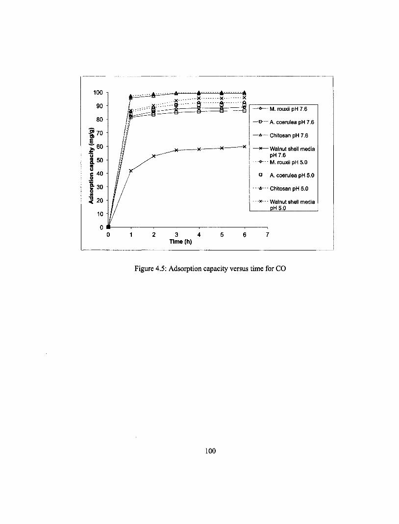
100
90
80
I s: 70 E
60
. 50 Uc 40 0 T.: IS 30
i < 20
10
0
--0-- M. rouxii pH 7.6
--e-- A. coerulea pH 7.6
--A-- Chitosan pH 7.6
x-- Walnut shell media pH 7.6
- - -0- - - M. rouxii pH 5.0
0 A. coerulea pH 5.0
---0--- Chitosan pH 5.0
- - -x- - - Walnut shell media pH 5.0
3 4 5 6 7 Time (h)
Figure 4.5: Adsorption capacity versus time for CO
100
• • • • » M. rouxii pH 7.6
—B— - A. coerulea pH 7.6
A— Chitosan pH 7.6
X— - Walnut shell media pH 7.6
- M. rouxii pH 5.0
• A. coerulea pH 5.0
- - A - - - Chitosan pH 5.0
- -X- - - Walnut shell media pH 5.0
2 3 4 Time (h)
Figure 4.5: Adsorption capacity versus time for CO
100

100
590
1.80
.970 o. co uc 60 o 150 0 to Q40
30
20
10
0 1 2 3 4
Time (h) 5
--4)-- M. rouxii pH 7.6
—a-- A. coerulea pH 7.6
--a-- Chitosan pH 7.6
-x-- Walnut shell media pH 7.6
- - -4- - - M. rouxii pH 5.0
---0-- - A. Coerulea pH 5.0
- --a- - - Chitosan pH 5.0
---x--- Walnut shell media pH 50
7
Figure 4.6: Adsorption capacity versus time for Bright-Edge 80
101
100
»90 ::
£
A a
-A
Q - •
X X -——X—
0 ..0 0 —-a— —a —B— —•
2 3 4 Time (h)
—0 M. rouxii pH 7.6
• A. coerulea pH 7.6
—a— - Chitosan pH 7.6
- Walnut shell media pH 7.6
- M. rouxii pH 5.0
—0- -- A. Coerulea pH 5.0
—A- - - Chitosan pH 5.0
—X- -- Walnut shell media DH 5.0
Figure 4.6: Adsorption capacity versus time for Bright-Edge 80
101

Table 4.6: Residual oil concentration obtained using different biomaterials
M rouxii A. coerulea Chitosan Walnut shell Oil Time, pH pH pH pH pH pH pH pH
h 7.6 5.0 7.6 5.0 7.6 5.0 7.6 5.0 SMO
1 75.6 65.7 88.0 72.6 26.6 17.3 150.7 67.7 2 72.0 57.3 82.0 64.5 23.7 12.2 142.0 49.3 3 69.1 46.8 79.1 55.8 13.3 5.0 135.1 35.6 4 66.9 45.8 78.1 55.4 9.1 2.1 128.0 33.8 5 66.3 45.8 77.6 55.6 9.6 1.2 118.1 34.1 6 66.0 45.6 78.0 55.8 9.2 0.8 123.9 35.0
CO 1 35.4 28.9 37.1 32.1 8.0 5.3 116.0 27.1 2 28.9 22.6 33.1 26.7 5.3 2.8 94.3 19.8 3 24.6 18.4 29.9 19.2 1.8 1.2 85.6 12.4 4 23.2 15.3 28.6 18.9 1.7 0.6 84.4 8.8 5 23.9 15.6 27.8 18.7 1.8 0.5 82.8 9.1 6 22.2 15.0 27.2 18.9 1.7 0.3 80.4 8.0
Bright-Edge 80 1 81.1 47.8 84.7 49.8 32.8 14.6 61.7 17.1 2 78.7 38.1 81.1 44.2 27.1 12.2 58.9 14.6 3 73.7 34.7 79.8 41.7 24.7 8.1 56.4 . 10.5 4 72.2 32.1 79.1 39.9 23.7 6.8 54.3 9.4 5 71.8 31.9 78.8 40.1 24.9 6.1 54.5 9.8 6 71.1 32.0 79.0 39.8 22.2 6.3 53.5 9.3
Note: All values 'n mg/L; initial oil concentration = 200 mg/L
102
Table 4.6: Residual oil concentration obtained using different biomaterials
M. rouxii A. coerulea Chitosan Walnut shell Oil Time, pH pH PH pH PH PH PH PH
h 7.6 5.0 7.6 5.0 7.6 5.0 7.6 5.0 SMO
1 75.6 65.7 88.0 72.6 26.6 17.3 150.7 67.7 2 72.0 57.3 82.0 64.5 23.7 12.2 142.0 49.3 3 69.1 46.8 79.1 55.8 13.3 5.0 135.1 35.6 4 66.9 45.8 78.1 55.4 9.1 2.1 128.0 33.8 5 66.3 45.8 77.6 55.6 9.6 1.2 118.1 34.1 6 66.0 45.6 78.0 55.8 9.2 0.8 123.9 35.0
CO 1 35.4 28.9 37.1 32.1 8.0 5.3 116.0 27.1 2 28.9 22.6 33.1 26.7 5.3 2.8 94.3 19.8 3 24.6 18.4 29.9 19.2 1.8 1.2 85.6 12.4 4 23.2 15.3 28.6 18.9 1.7 0.6 84.4 8.8 5 23.9 15.6 27.8 18.7 1.8 0.5 82.8 9.1 6 22.2 15.0 27.2 18.9 1.7 0.3 80.4 8.0
Bright-Edge 8( 1 81.1 47.8 84.7 49.8 32.8 14.6 61.7 17.1 2 78.7 38.1 81.1 44.2 27.1 12.2 58.9 14.6 3 73.7 34.7 79.8 41.7 24.7 8.1 56.4 10.5 4 72.2 32.1 79.1 39.9 23.7 6.8 54.3 9.4 5 71.8 31.9 78.8 40.1 24.9 6.1 54.5 9.8 6 71.1 32.0 79.0 39.8 22.2 6.3 53.5 9.3
Note: All values in mg/L; initial oil concentration = 200 mg/L
102

Each batch test was conducted in triplicate and the mean is represented by one data point
in the figures. The deviations of the three points from the mean were found to be within
±1%; the standard deviation for each set of data was found to be relatively small
compared to the mean. Among the three oils studied, maximum oil removals were
observed in the case of canola oil for all four adsorbents (Table 4.7). The adsorption
capacities for canola oil at pH 5.0 were 92.5, 90.5, 99.9, and 96 mg/g by M rouxii, A.
coerulea, chitosan and walnut shell media, respectively. This could be due to the fact that
in comparison with the other two emulsions, vegetable oil emulsions are known for their
limited stability (Vesala et al. 1985). Vegetable oils predominantly consist of
triglycerides (Pushkarev et al. 1983) and emulsions based on oils from the triglyceride
group showed poor stability in comparison with emulsions based on hydrocarbon oils
(Ozgen et al. 2006). At pH 5.0, minimum oil removal was obtained in the case of Bright-
Edge 80 using the four adsorbents studied. Bright-Edge 80 cutting oil is the one with the
least interfacial tension among the oils studied. Low interfacial tension would result in
reduced free surface energy associated with the formation of droplets. It enhances the
formation of smaller emulsion droplets with greater kinetic stability (Aserin 2007). Better
oil removals for all three oils were obtained at pH 5.0 than at pH 7.6 for all four
adsorbents. According to Figure 4.1, in the case of all three oils, the zeta-potential value
was less electronegative at pH 5.0 when compared to that at pH 7.0. Zeta-potential
indicates the stability of oil-in-water emulsions. A higher magnitude of zeta-potential
would refer to greater forces of repulsion between particles in the emulsion, which would
lead to better stability of the emulsions (Reynolds and Richards 1995). With a decrease in
103
Each batch test was conducted in triplicate and the mean is represented by one data point
in the figures. The deviations of the three points from the mean were found to be within
±1%; the standard deviation for each set of data was found to be relatively small
compared to the mean. Among the three oils studied, maximum oil removals were
observed in the case of canola oil for all four adsorbents (Table 4.7). The adsorption
capacities for canola oil at pH 5.0 were 92.5, 90.5, 99.9, and 96 mg/g by M. rouxii, A,
coerulea, chitosan and walnut shell media, respectively. This could be due to the fact that
in comparison with the other two emulsions, vegetable oil emulsions are known for their
limited stability (Vesala et al. 1985). Vegetable oils predominantly consist of
triglycerides (Pushkarev et al. 1983) and emulsions based on oils from the triglyceride
group showed poor stability in comparison with emulsions based on hydrocarbon oils
(Ozgen et al. 2006). At pH 5.0, minimum oil removal was obtained in the case of Bright-
Edge 80 using the four adsorbents studied. Bright-Edge 80 cutting oil is the one with the
least interfacial tension among the oils studied. Low interfacial tension would result in
reduced free surface energy associated with the formation of droplets. It enhances the
formation of smaller emulsion droplets with greater kinetic stability (Aserin 2007). Better
oil removals for all three oils were obtained at pH 5.0 than at pH 7.6 for all four
adsorbents. According to Figure 4.1, in the case of all three oils, the zeta-potential value
was less electronegative at pH 5.0 when compared to that at pH 7.0. Zeta-potential
indicates the stability of oil-in-water emulsions. A higher magnitude of zeta-potential
would refer to greater forces of repulsion between particles in the emulsion, which would
lead to better stability of the emulsions (Reynolds and Richards 1995). With a decrease in
103

Table 4.7: Oil removals by biomaterials
Oil removals, % Oil pH M rouxii A. coerulea Chitosan Walnut shell SMO 7.6 67 61 96 38
5.0 77 72 99 83 CO 7.6 89 87 99 60
5.0 93 91 99 96 Bright-Edge 80 7.6 65 61 89 73
5.0 84 80 97 96 Note: Initial concentration = 200 mg/L; Time of contact = 6 h; Adsorbent dose = 0.2 g.
104
Table 4.7: Oil removals by biomaterials
Oil removals, % Oil PH M. rouxii A. coerulea Chitosan Walnut shell SMO 7.6 67 61 96 38
5.0 77 72 99 83 CO 7.6 89 87 99 60
5.0 93 91 99 96 Bright-Edge 80 7.6 65 61 89 73
5.0 84 80 97 96 Note: Initial concentration = 200 mg/L; Time of contact = 6 h; Adsorbent dose = 0.2 g.
104

the magnitude of zeta-potential, the possibility of coagulation of dispersed particles
increases and the emulsion becomes less stable (Riddick 1968; Pushkarev et al. 1983).
Hence, a lower electro-negativity value of pH 5.0 for the three oils studied resulted in
higher removal efficiency. Similar behavior was found by Ahmad et al. (2005a) with
chitosan, which was used to remove residue oil from POME. They observed that when
the pH was lower than 5.0, the percentage of residue oil adsorption could be increased to
99%. Also, at a pH of more than 5.0, the percentage of adsorption was found to decrease
and when the pH was 7.0, the percentage of residue oil adsorption was the lowest. Similar
trends were observed with bentonite and activated carbon which, when used for
adsorption of residue oil from POME, showed a higher oil removal at a pH of less than
5.0 (Ahmad et al. 2005b). It was suggested that the acidic conditions acted as a catalyst to
catalyze the reaction between the residue oil molecules and the adsorption site of chitosan
(-NH2 group) (Ahmad et al. 2005a). In the case of fungal biomass, their surfaces have
been generally observed to be negatively charged because of the ionization of functional
groups present (Yan and Viraraghavan 2003). At acidic pH, some of the functional
groups present in the fungal cell wall will be positively charged and the negative charge
intensity on the sites will be reduced, which might have an effect on the sorption
characteristics of the biomass (Yan and Viraraghavan 2003). Uptake by dead fungal cells
takes place as a result of the functional groups of the cell and, in particular, the cell wall.
The mechanism of uptake by the cell wall has been broadly categorized as: (1) uptake
directed by functional groups such as phosphate, carboxyl, amine and phosphate diester
species of the compounds; and (2) physio-chemical interactions directed by adsorption
105

phenomena (Kapoor and Viraraghavan 1995). Biosorption mechanisms have been found
to include ion-exchange, co-ordination, complexation, chelation, adsorption and
microprecipitation (Yan and Viraraghavan 2000). At this stage, it is necessary to carry
out more detailed studies to understand the specific mechanism involved in the
biosorption of oil by fungal adsorbents. The mechanism of oil removal in the case of
walnut shell media has been observed to be sorption (Rahman 1992). Oil is found at the
interstices of the finely divided granules of the walnut shell media, which was observed
to be an excellent coalescing material.
Among the two fungal biomasses studied, M rouxii was found to be better for oil
sorption than A. coerulea. The adsorption capacity of M rouxii at pH 5.0 for SMO,
canola oil and Bright-Edge 80 were 77.2, 92.5, and 84 mg/g, respectively. The higher
adsorption capacity for oil by M rouxii, when compared to A. coerulea, could be due to
its higher BET surface area. Most adsorbents with a higher surface area have been found
to facilitate adsorption of residue oil (Ahmad et al. 2005a). Mycelium of M rouxii grows
in the form of suspended' growth leading to a larger surface area of the biomass for
adsorption (Yan and Viraraghavan 2000). In the case of A. coerulea, it grows in the form
of pellets with a lower surface area. Most Absidia species are found to have a strong
inclination to form pellets during their growth in a fermenter (Davoust and Persson
1992). Yan and Viraraghavan (2000) have observed that the biosorption capacity of
heavy metals were higher for M rouxii than for A. niger and the difference was ascribed
to the larger surface area of M rouxii. The effectiveness of M rouxii in removing the oils
follows this order: CO, SMO, and Bright-Edge 80. The oil adsorption capacity by M
106
phenomena (Kapoor and Viraraghavan 1995). Biosorption mechanisms have been found
to include ion-exchange, co-ordination, complexation, chelation, adsorption and
microprecipitation (Yan and Viraraghavan 2000). At this stage, it is necessary to carry
out more detailed studies to understand the specific mechanism involved in the
biosorption of oil by fungal adsorbents. The mechanism of oil removal in the case of
walnut shell media has been observed to be sorption (Rahman 1992). Oil is found at the
interstices of the finely divided granules of the walnut shell media, which was observed
to be an excellent coalescing material.
Among the two fungal biomasses studied, M. rouxii was found to be better for oil
sorption than A. coerulea. The adsorption capacity of M. rouxii at pH 5.0 for SMO,
canola oil and Bright-Edge 80 were 77.2, 92.5, and 84 mg/g, respectively. The higher
adsorption capacity for oil by M. rouxii, when compared to A. coerulea, could be due to
its higher BET surface area. Most adsorbents with a higher surface area have been found
to facilitate adsorption of residue oil (Ahmad et al. 2005a). Mycelium of M. rouxii grows
in the form of suspended growth leading to a larger surface area of the biomass for
adsorption (Yan and Viraraghavan 2000). In the case of A. coerulea, it grows in the form
of pellets with a lower surface area. Most Absidia species are found to have a strong
inclination to form pellets during their growth in a fermenter (Davoust and Persson
1992). Yan and Viraraghavan (2000) have observed that the biosorption capacity of
heavy metals were higher for M. rouxii than for A. niger and the difference was ascribed
to the larger surface area of M. rouxii. The effectiveness of M. rouxii in removing the oils
follows this order: CO, SMO, and Bright-Edge 80. The oil adsorption capacity by M.
106

rouxii was lower when compared with that of crab shell chitosan. However, M rouxii is
found to contain approximately 32% of chitosan in its cell wall (Bartnicki-Garcia and
Nickerson 1962, exhibiting an adsorption capacity of 92.5 mg/g for canola oil at pH 5.0
while pure chitosan showed an adsorption capacity of 99.9 mg/g. Oil uptake by M rouxii
is also influenced by other functional groups present in the cell wall.
4.5 Factorial Design of Experiments
The design matrix of uncoded values for the factors and the response in terms of
the percent removal of SMO, CO and Bright-Edge 80 for all experimental runs including
replicates, are shown in Table 4.8. A linear regression model was fitted for the
experimental data using the least square technique using MINITAB. The model
coefficients for the removal, the effects and standardized effects of the factors and
interactions, and p-values of the effects in the model are shown in Tables 4.9 - 4.11 for
SMO, CO, and Bright-Edge 80, respectively. The net effect is a difference between the
responses of two levels (high and low level) of factors; the regression model coefficients
are obtained by dividing the net effects by two. The standardized effects are obtained by
dividing the regression coefficients by standard error coefficient (Antony, 2003). The p-
value is the probability value used to determine the effects in the model that are
statistically significant. P-value is termed as the probability that measures the strength of
the evidence against a null hypothesis (Moore, 2009). As for a 95% confidence level, the
p-value should be less than or equal to 0.05 (0 < 0.05) for the effect to be statistically
significant.
107
rouxii was lower when compared with that of crab shell chitosan. However, M, rouxii is
found to contain approximately 32% of chitosan in its cell wall (Bartnicki-Garcia and
Nickerson 1962, exhibiting an adsorption capacity of 92.5 mg/g for canola oil at pH 5.0
while pure chitosan showed an adsorption capacity of 99.9 mg/g. Oil uptake by M. rouxii
is also influenced by other functional groups present in the cell wall.
4.5 Factorial Design of Experiments
The design matrix of uncoded values for the factors and the response in terms of
the percent removal of SMO, CO and Bright-Edge 80 for all experimental runs including
replicates, are shown in Table 4.8. A linear regression model was fitted for the
experimental data using the least square technique using MINITAB. The model
coefficients for the removal, the effects and standardized effects of the factors and
interactions, and /^-values of the effects in the model are shown in Tables 4.9 - 4.11 for
SMO, CO, and Bright-Edge 80, respectively. The net effect is a difference between the
responses of two levels (high and low level) of factors; the regression model coefficients
are obtained by dividing the net effects by two. The standardized effects are obtained by
dividing the regression coefficients by standard error coefficient (Antony, 2003). The p-
value is the probability value used to determine the effects in the model that are
statistically significant. P-value is termed as the probability that measures the strength of
the evidence against a null hypothesis (Moore, 2009). As for a 95% confidence level, the
p-value should be less than or equal to 0.05 (0 < 0.05) for the effect to be statistically
significant.
107

Table 4.8: Uncoded design table for the factors and response
Run pH Temp- erature
(°C)
Dose (g)
Conc- entration (mg/L)
Speed (rpm)
% removal of SMO
% removal of CO
% removal
of Bright-Edge 80
1 3 5 0.05 350 100 99.90 99.97 99.90 2 3 5 0.50 50 100 80.20 99.40 89.14 3 9 30 0.05 50 200 38.00 54.00 87.60 4 3 5 0.05 50 200 94.80 99.60 91.80 5 9 5 0.50 50 200 27.00 59.60 68.80 6 9 5 0.50 350 100 51.70 46.80 13.40 7 9 30 0.50 50 100 60.00 61.60 57.40 8 3 30 0.50 50 200 96.40 98.00 88.20 9 3 5 0.50 350 200 99.77 99.77 98.80 10 9 5 0.05 350 200 9.10 23.10 8.00 11 9 30 0.50 350 200 58.00 79.70 69.40 12 9 30 0.05 50 200 39.10 56.00 88.00 13 9 5 0.05 50 100 23.40 90.40 44.60 14 3 30 0.50 50 200 96.70 97.70 88.00 15 3 5 0.05 350 100 99.70 99.80 99.10 16 3 30 0.05 350 200 98.40 99.80 99.60 17 3 30 0.05 50 100 99.60 99.80 90.60 18 9 5 0.50 50 200 28.00 60.10 68.90 19 9 30 0.50 350 200 58.40 80.10 70.00 20 3 5 0.50 50 100 80.60 99.60 89.90 21 3 30 0.05 50 100 99.50 99.30 91.00 22 3 30 0.50 350 100 97.40 97.90 97.00 23 9 5 0.50 350 100 52.00 47.10 14.20 24 3 5 0.50 350 200 99.40 98.60 98.60 25 3 30 0.05 350 200 98.80 99.70 99.30 26 9 30 0.05 350 100 37.10 55.40 36.80 27 9 5 0.05 50 100 25.00 91.00 44.40 28 9 30 0.05 350 100 37.40 55.10 37.20 29 3 30 0.50 350 100 97.70 97.20 97.20 30 9 30 0.50 50 100 61.20 62.00 58.00 31 9 5 0.05 350 200 10.00 22.80 9.00 32 3 5 0.05 50 200 95.10 99.40 92.00
108
Table 4.8: Uncoded design table for the factors and response
Run PH Temp Dose Conc Speed % % % erature (g) entration (rpm) removal removal removal
(°C) (mg/L) ofSMO of CO of Bright-Edge 80
1 3 5 0.05 350 100 99.90 99.97 99.90 2 3 5 0.50 50 100 80.20 99.40 89.14 3 9 30 0.05 50 200 38.00 54.00 87.60 4 3 5 0.05 50 200 94.80 99.60 91.80 5 9 5 0.50 50 200 27.00 59.60 68.80 6 9 5 0.50 350 100 51.70 46.80 13.40 7 9 30 0.50 50 100 60.00 61.60 57.40 8 3 30 0.50 50 200 96.40 98.00 88.20 9 3 5 0.50 350 200 99.77 99.77 98.80 10 9 5 0.05 350 200 9.10 23.10 8.00 11 9 30 0.50 350 200 58.00 79.70 69.40 12 9 30 0.05 50 200 39.10 56.00 88.00 13 9 5 0.05 50 100 23.40 90.40 44.60 14 3 30 0.50 50 200 96.70 97.70 88.00 15 3 5 0.05 350 100 99.70 99.80 99.10 16 3 30 0.05 350 200 98.40 99.80 99.60 17 3 30 0.05 50 100 99.60 99.80 90.60 18 9 5 0.50 50 200 28.00 60.10 68.90 19 9 30 0.50 350 200 58.40 80.10 70.00 20 3 5 0.50 50 100 80.60 99.60 89.90 21 3 30 0.05 50 100 99.50 99.30 91.00 22 3 30 0.50 350 100 97.40 97.90 97.00 23 9 5 0.50 350 100 52.00 47.10 14.20 24 3 5 0.50 350 200 99.40 98.60 98.60 25 3 30 0.05 350 200 98.80 99.70 99.30 26 9 30 0.05 350 100 37.10 55.40 36.80 27 9 5 0.05 50 100 25.00 91.00 44.40 28 9 30 0.05 350 100 37.40 55.10 37.20 29 3 30 0.50 350 100 97.70 97.20 97.20 30 9 30 0.50 50 100 61.20 62.00 58.00 31 9 5 0.05 350 200 10.00 22.80 9.00 32 3 5 0.05 50 200 95.10 99.40 92.00
108

Table 4.9: Estimated effects and coefficients for the removal of SMO (% coded units)
Term Net effect
Regression coefficient
Standardized effect (T)
p-value
Constant 67.17 753.50 0.000
pH -57.41 -28.71 -322.02 0.000
Temperature 12.38 6.19 69.42 0.000
Dose 8.72 4.36 48.93 0.000
Concentration 3.76 1.88 21.09 0.000
Speed -3.46 -1.73 -19.43 0.000
pH*Temperature 8.00 4.00 44.86 0.000
pH*Dose 13.43 6.71 75.31 0.000
pH*Concentration -2.26 -1.13 -12.68 0.000
pH*speed -6.56 -3.28 -36.80 0.000
Temperature*Dose 1.01 0.51 5.69 0.000
Temperature*Concentration -4.67 -2.34 -26.21 0.000
Temperature*speed 2.70 1.35 15.15 0.000
Dose*Concentration 6.77 3.39 37.99 0.000
Dose*speed 1.32 0.66 7.42 0.000
Concentration*speed -1.66 -0.83 -9.34 0.000
Note: Standard error coefficient for all cases = 0.08914
109
Table 4.9: Estimated effects and coefficients for the removal of SMO (% coded units)
Term Net effect
Regression coefficient
Standardized effect (T)
p-v alue
Constant 67.17 753.50 0.000
PH -57.41 -28.71 -322.02 0.000
Temperature 12.38 6.19 69.42 0.000
Dose 8.72 4.36 48.93 0.000
Concentration 3.76 1.88 21.09 0.000
Speed -3.46 -1.73 -19.43 0.000
pH*Temperature 8.00 4.00 44.86 0.000
pH*Dose 13.43 6.71 75.31 0.000
pH*Concentration -2.26 -1.13 -12.68 0.000
pH*speed -6.56 -3.28 -36.80 0.000
Temperature ""Dose 1.01 0.51 5.69 0.000
Temperature*Concentration -4.67 -2.34 -26.21 0.000
T emperature* speed 2.70 1.35 15.15 0.000
Dose* Concentration 6.77 3.39 37.99 0.000
Dose*speed 1.32 0.66 7.42 0.000
Concentration* speed -1.66 -0.83 -9.34 0.000
Note: Standard error coefficient for all cases = 0.08914
109

Table 4.10: Estimated effects and coefficients for the removal of CO (% coded units)
Term Net effect
Regression coefficient
Standardized effect (T)
p-value
Constant 79.07 922.86 0.000
pH -40.05 -20.02 -233.69 0.000
Temperature 3.52 1.76 20.52 0.000
Dose 2.50 1.25 14.59 0.000
Concentration -7.79 -3.90 -45.47 0.000
Speed -4.65 -2.32 -27.13 0.000
pH*Temperature 4.36 2.18 25.44 0.000
pH*Dose 3.65 1.83 21.30 0.000
pH*Concentration -7.78 -3.89 -45.42 0.000
pH*Speed -4.60 -2.30 -26.84 0.000
Temperature*Dose 4.39 2.19 25.60 0.000
Temperature*Concentration 12.35 6.18 72.09 0.000
Temperature*Speed 9.24 4.62 53.90 0.000
Dose*Concentration 8.94 4.47 52.15 0.000
Dose*Speed 12.40 6.20 72.34 0.000
Concentration*Speed 5.19 2.59 30.27 0.000
Note: Standard error coefficient for all cases = 0.08568
110
Table 4.10: Estimated effects and coefficients for the removal of CO (% coded units)
Term Net Regression Standardized p-value effect coefficient effect (T)
Constant 79.07 922.86 0.000
pH -40.05 -20.02 -233.69 0.000
Temperature 3.52 1.76 20.52 0.000
Dose 2.50 1.25 14.59 0.000
Concentration -7.79 -3.90 -45.47 0.000
Speed -4.65 -2.32 -27.13 0.000
pH*Temperature 4.36 2.18 25.44 0.000
pH*Dose 3.65 1.83 21.30 0.000
pH*Concentration -7.78 -3.89 -45.42 0.000
pH* Speed -4.60 -2.30 -26.84 0.000
Temperature * Dose 4.39 2.19 25.60 0.000
T emperature * Concentration 12.35 6.18 72.09 0.000
Temperature*Speed 9.24 4.62 53.90 0.000
Dose* Concentration 8.94 4.47 52.15 0.000
Dose* Speed 12.40 6.20 72.34 0.000
Concentration* Speed 5.19 2.59 30.27 0.000
Note: Standard error coefficient for all cases = 0.08568
110
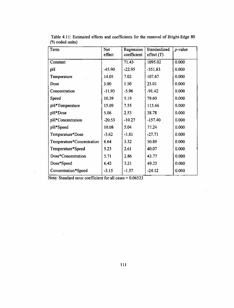
Table 4.11: Estimated effects and coefficients for the removal of Bright-Edge 80 (% coded units)
Term Net effect
Regression coefficient
Standardized effect (T)
p-value
Constant 71.43 1095.02 0.000
pH -45.90 -22.95 -351.83 0.000
Temperature 14.05 7.02 107.67 0.000
Dose 3.00 1.50 23.01 0.000
Concentration -11.93 -5.96 -91.42 0.000
Speed 10.39 5.19 79.60 0.000
pH*Temperature 15.09 7.55 115.66 0.000
pH*Dose 5.06 2.53 38.78 0.000
pH*Concentration -20.53 -10.27 -157.40 0.000
pH*Speed 10.08 5.04 77.24 0.000
Temperature*Dose -3.62 -1.81 -27.71 0.000
Temperature*Concentration 6.64 3.32 50.89 0.000
Temperature*Speed 5.23 2.61 40.07 0.000
Dose*Concentration 5.71 2.86 43.77 0.000
Dose*Speed 6.42 3.21 49.23 0.000
Concentration*Speed -3.15 -1.57 -24.12 0.000
Note: Standard error coefficient for all cases = 0.06523
111
Table 4.11: Estimated effects and coefficients for the removal of Bright-Edge 80 (% coded units)
Term Net Regression Standardized p-value effect coefficient effect (T)
Constant 71.43 1095.02 0.000
pH -45.90 -22.95 -351.83 0.000
Temperature 14;05 7.02 107.67 0.000
Dose 3.00 1.50 23.01 0.000
Concentration -11.93 -5.96 -91.42 0.000
Speed 10.39 5.19 79.60 0.000
pH*Temperature 15.09 7.55 115.66 0.000
pH*Dose 5.06 2.53 38.78 0.000
pH*Concentration -20.53 -10.27 -157.40 0.000
pH* Speed 10.08 5.04 77.24 0.000
Temperature *Dose -3.62 -1.81 -27.71 0.000
Temperature * Concentration 6.64 3.32 50.89 0.000
Temperature * Speed 5.23 2.61 40.07 0.000
Dose*Concentration 5.71 2.86 43.77 0.000
Dose*Speed 6.42 3.21 49.23 0.000
Concentration* Speed -3.15 -1.57 -24.12 0.000
Note: Standard error coefficient for all cases = 0.06523
111

A statistical analysis (normal probability plot) of the data in terms of the standardized
residual was also conducted to verify the normality of the data. The absolute value of the
estimated effect determines its relative strength over the response. The higher the value of
the effect, the higher the influence over the response. The significance level for this
model was chosen to be 0.05 (95% confidence level). Solution pH had the highest effect
on the removal of all three oils. A negative sign of the effect indicates that a low factor
setting (-1) would result in a higher removal (Minitab 2007). A decrease in solution pH to
3.0 from 9.0 increased the percent removal of SMO, CO and Bright-Edge 80 to as high as
99%. It was found that pH 3.0 is the point at which the zeta-potential of autoclaved M
rouxii was zero. Acidic pH has been found to increase the percentage of residue oil
adsorption to 99% according to Ahmad et al (2005a). Similar trends were observed with
bentonite and activated carbon which when used for adsorption of residue oil from
POME, showed higher oil removal at a pH of less than 5.0 (Ahmad et al 2005b). As for
the removal of SMO, the magnitude of effects of each factor and their interactions were
found to increase in the following order: pH > pH*Dose > Temperature. With respect to
the removal of CO, the increasing order of the effects was given by: pH > Dose*Speed >
Temperature*Concentration. Bright-Edge 80, was given by: pH > pH*Concentration >
pH*Temperature > Temperature. The p-values in the estimated effects and coefficients
were used to determine statistically significant individual and interaction effects. All
factors or combination of factors were found to be statistically significant (p-values <
0.05) for the removal of SMO, CO and Bright-Edge 80.
112
A statistical analysis (normal probability plot) of the data in terms of the standardized
residual was also conducted to verify the normality of the data. The absolute value of the
estimated effect determines its relative strength over the response. The higher the value of
the effect, the higher the influence over the response. The significance level for this
model was chosen to be 0.05 (95% confidence level). Solution pH had the highest effect
on the removal of all three oils. A negative sign of the effect indicates that a low factor
setting (-1) would result in a higher removal (Minitab 2007). A decrease in solution pH to
3.0 from 9.0 increased the percent removal of SMO, CO and Bright-Edge 80 to as high as
99%. It was found that pH 3.0 is the point at which the zeta-potential of autoclaved M.
rouxii was zero. Acidic pH has been found to increase the percentage of residue oil
adsorption to 99% according to Ahmad et al (2005a). Similar trends were observed with
bentonite and activated carbon which when used for adsorption of residue oil from
POME, showed higher oil removal at a pH of less than 5.0 (Ahmad et al 2005b). As for
the removal of SMO, the magnitude of effects of each factor and their interactions were
found to increase in the following order: pH > pH*Dose > Temperature. With respect to
the removal of CO, the increasing order of the effects was given by: pH > Dose*Speed >
Temperature*Concentration. Bright-Edge 80, was given by: pH > pH*Concentration >
pH * Temperature > Temperature. The /^-values in the estimated effects and coefficients
were used to determine statistically significant individual and interaction effects. All
factors or combination of factors were found to be statistically significant (p-values <
0.05) for the removal of SMO, CO and Bright-Edge 80.
112

4.5.1 Pareto Plot of Effect
The Pareto plot visually represents the absolute values of the effects of the main
factors and the effects of the interaction of factors. A reference line is drawn to indicate
the factors, which extend past this line, are potentially important (Antony 2003). pH had
the greatest effect on the removal for all three oils (Figures 4.7 - 4.9). In the figures, the
reference line can be found near the vertical axis. The effects above the reference line are
statistically significant at a 95% confidence level and all effects were found to be
statistically significant. The relative importance of each factor and the combination of
factors can be observed according to the Pareto plots for all three oils.
4.5.2 Main Effects Plot
The main effects plot is shown in Figures 4.10 — 4.12 with respect to the removal
of SMO, CO, and Bright-Edge 80, respectively. It indicates the relative strength of the
effects of various factors. A main effect is present when the mean response changes
across the level of a factor. The sign of the main effect indicates the directions of the
effect. It can be observed from the main effects plot that for all three oils, the effect of pH
was characterized by a greater degree of departure from the overall mean. The pH had a
negative effect upon the removal of all three oils. For SMO, temperature and dose
showed a slight positive effect upon removal. As for CO, the concentration had a slight
negative effect upon removal. With respect to the Bright-Edge 80, temperature and speed
had a slight positive effect while concentration was found to have a slight negative effect.
All other factors showed a smaller change. The patterns were previously identified by
113
4.5.1 Pareto Plot of Effect
The Pareto plot visually represents the absolute values of the effects of the main
factors and the effects of the interaction of factors. A reference line is drawn to indicate
the factors, which extend past this line, are potentially important (Antony 2003). pH had
the greatest effect on the removal for all three oils (Figures 4.7 - 4.9). In the figures, the
reference line can be found near the vertical axis. The effects above the reference line are
statistically significant at a 95% confidence level and all effects were found to be
statistically significant. The relative importance of each factor and the combination of
factors can be observed according to the Pareto plots for all three oils.
4.5.2 Main Effects Plot
The main effects plot is shown in Figures 4.10-4.12 with respect to the removal
of SMO, CO, and Bright-Edge 80, respectively. It indicates the relative strength of the
effects of various factors. A main effect is present when the mean response changes
across the level of a factor. The sign of the main effect indicates the directions of the
effect. It can be observed from the main effects plot that for all three oils, the effect of pH
was characterized by a greater degree of departure from the overall mean. The pH had a
negative effect upon the removal of all three oils. For SMO, temperature and dose
showed a slight positive effect upon removal. As for CO, the concentration had a slight
negative effect upon removal. With respect to the Bright-Edge 80, temperature and speed
had a slight positive effect while concentration was found to have a slight negative effect.
All other factors showed a smaller change. The patterns were previously identified by

Pareto Chart of the Standardized Effects (response is % Removal, Alpha = 0.05)
2..1 A
AC
B
C AB
CD AE BD D
E
BE AD DE
CE BC
0 50 100 150 200 250 Standardized Effect
300 350
Factor Name A pH B Temperature C Dose D Concentration E speed
Figure 4.7: Pareto chart for standardized effects for the removal of SMO
114
Pareto Chart of the Standardized Effects (response is % Removal, Alpha = 0.05)
2.1 Factor Name A PH B Temperature C Dose
D Concentration E speed
CD-
0 50 100 150 200 250 300 350 Standardized Effect
Figure 4.7: Pareto chart for standardized effects for the removal of SMO
114

Pareto Chart of the Standardized Effects (response is % Removal, Alpha = 0.05)
2.1 A
CE
BD BE CD
D AD DE
AE
BC AB AC
B
0 50 100 150 Standardized Effect
200 250
Factor Name A pH B Temperature C Dose D Concentration E Speed
Figure 4.8: Pareto chart for standardized effects for the removal of CO
115
[2
2.1
A
CE
BD
BE
CD
D
AD
DE
E
AE
BC
AB
AC
B
C
Pareto Chart of the Standardized Effects (response is % Removal, Alpha = 0.05)
~50 100 150 Standardized Effect
Factor Name A PH B Temperature C Dose D Concentration E Speed
200 *250
Figure 4.8: Pareto chart for standardized effects for the removal of CO
115

Pareto Chart of the Standardized Effects (response is % Removal, Alpha = 0.05)
1
2.1 A
AD
AB B D
E AE BD CE
CD BE
AC sc DE
C
0 . I
100 200 300 Standardized Effect
400
Factor Name A pH B Temperature C Dose D Concentration E Speed
Figure 4.9: Pareto chart for standardized effects for the removal of Bright-Edge 80
116
2.1
A AO
AB
B D E
AE
BD
CE CD BE
AC
BC
DE C
w
Pareto Chart of the Standardized Effects (response is % Removal, Alpha = 0.05)
1
loo"
Factor Name A PH B Temperature C Dose D Concentration E Speed
200 300 Standardized Effect
"400
Figure 4.9: Pareto chart for standardized effects for the removal of Bright-Edge 80
116

Main Effects Plot for % Removal Data Means
100
80
60
C 40
i 100
80
60
40
pH Temperature Dose
_.-----.
\
•- e-----
3 5 Concentration speed
•
50 350 100 200
0.
Figure 4.10: Main effects plot for the removal of SMO
117
o.
Main Effects Plot for % Removal Data Means
Temperature Dose 100-
80-
60-
40-c
i 0.05 0.50
speed Concentration 100-
80-
60-
50 350 100 200
Figure 4.10: Main effects plot for the removal of SMO
117

Main Effects Plot for % Removal Data Means
100
90
80
70
60
pH Temperature Dose
3 9
100-
90-
80-
70-
60-
Concentration Speed
50 350 100 200
0.05
Figure 4.11: Main effects plot for the removal of CO
118
0.50
Main Effects Plot for % Removal Data Means
Concentration
Figure 4.11: Main effects plot for the removal of CO
118
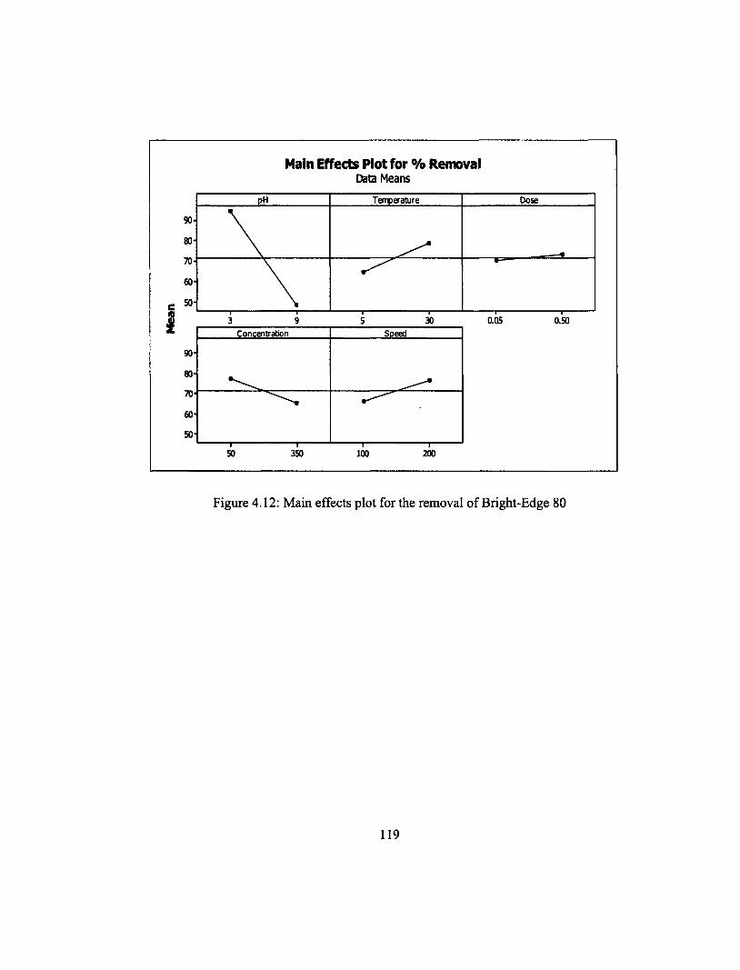
Main Effects Plot for % Removal Data Means
C
i
90
80
70
60
50
90
80
70
60
50
pH Temperature Dose
—,=,",-----'°---.
\
•--' .. . .'a
3 Concentration Speed
.----'--.
50 350 100 200
0.05 0.50
Figure 4.12: Main effects plot for the removal of Bright-Edge 80
119
Main Effects Plot for % Removal Data Means
Temperature Dose
90-
80-
70-
60-
0.05 0.50
Speed Concentration
90-
80-
70-
60-
50-
50 350 100 200
Figure 4.12: Main effects plot for the removal of Bright-Edge 80
119

statistical significance. Statistical analysis of experimental data showed the effects of the
factors upon removal percentage of the three oils were not similar. This could be due to
the fact that the composition of the three oil-in-water emulsions used in the study was
different.
4.5.3 Interaction Effects Plot
The interaction effects plots are shown in Figures 4.13 — 4.15 for the removal of
SMO, CO, and Bright-Edge 80, respectively. The plots provide the mean response of two
factors at all possible combinations of their settings. If the lines are not parallel, it is an
indication of interaction between the two factors (Antony 2003). The interaction plots for
all three oils showed the pH interacted strongly with all other factors indicating pH to be
a predominant influencing factor in removal. A decrease in the solution pH to 3.0
increased the percent removal of the oils. The concentration of SMO and the dose of the
adsorbent showed a minor interaction with each other (Figure 4.13). When an adsorbent
dose of 0.5 g was used, the percent removal of SMO decreased at a SMO concentration
of 50 mg/L and the percent removal of SMO increased at a SMO concentration of 350
mg/L. Percent removal of SMO appeared not to be affected at a low dose of 0.05 g,
irrespective of the SMO concentration. A higher removal of SMO was observed at a dose
of 0.5 g for both concentrations than at a dose of 0.05 g. Adsorbent dose was previously
found to be statistically significant in the removal of SMO. As for CO, combinations of
the adsorbent dose and the rotational speed, solution temperature and rotational speed,
120
statistical significance. Statistical analysis of experimental data showed the effects of the
factors upon removal percentage of the three oils were not similar. This could be due to
the fact that the composition of the three oil-in-water emulsions used in the study was
different.
4.5.3 Interaction Effects Plot
The interaction effects plots are shown in Figures 4.13-4.15 for the removal of
SMO, CO, and Bright-Edge 80, respectively. The plots provide the mean response of two
factors at all possible combinations of their settings. If the lines are not parallel, it is an
indication of interaction between the two factors (Antony 2003). The interaction plots for
all three oils showed the pH interacted strongly with all other factors indicating pH to be
a predominant influencing factor in removal. A decrease in the solution pH to 3.0
increased the percent removal of the oils. The concentration of SMO and the dose of the
adsorbent showed a minor interaction with each other (Figure 4.13). When an adsorbent
dose of 0.5 g was used, the percent removal of SMO decreased at a SMO concentration
of 50 mg/L and the percent removal of SMO increased at a SMO concentration of 350
mg/L. Percent removal of SMO appeared not to be affected at a low dose of 0.05 g,
irrespective of the SMO concentration. A higher removal of SMO was observed at a dose
of 0.5 g for both concentrations than at a dose of 0.05 g. Adsorbent dose was previously
found to be statistically significant in the removal of SMO. As for CO, combinations of
the adsorbent dose and the rotational speed, solution temperature and rotational speed,
120

Interaction Plot for % Removal Data Means
Figure 4.13: Interaction effects plot for the removal of SMO
121
Interaction Plot for % Removal Data Means
30 0,05 0,^0 SO 3y 100 2g0
w .s*
W
•- *
*- » ft-
"" *•«
*- • •— — Hi i I
"
Dole
-III
Concentration —
PH
• 3
-m- 9
Temperature
m 5
-m- 30
Dose
0.05
—*- 0.50
Concentration
50
350
Figure 4.13: Interaction effects plot for the removal of SMO
121

Interaction Plot for % Removal Data Means
Figure 4.14: Interaction effects plot for the removal of CO
122
Interaction Plot for % Removal Data Means
J 0.(15 Q.ft) 2 2L 200
wr
Tmpanhn ^
f :
DOM
Concvtattn
PH
3
9
Temperature
5
30
Dose
m 0.05
0.50
Concentration
50
-9- 350
Figure 4.14: Interaction effects plot for the removal of CO
122

Figure 4.15: Interaction effects plot for the removal of Bright-Edge 80
123
Interaction Plot for % Removal Data Means
PH
J 2L
Tupwhw
0.05 OfO
DMI
100 29a -100
pH
• 75 • 3
-50 9
-100 -100 Temperature
•75 • 5
-50 30
-100 Dose
-75 —•— 0.05
-50 —Wr~ 0.50
- 100 - 100 Concentration
k 75 m 50
-so 350
Figure 4.15: Interaction effects plot for the removal of Bright-Edge 80
123

solution temperature and CO concentration and adsorbent dose and CO concentration
showed antagonistic effects (Figure 4.14). The concentration of CO and solution
temperature showed a slight interaction with each other. The percent removal of CO was
not affected by the rotational speed at a CO concentration of 350 mg/L while the percent
removal of CO increased at a CO concentration of 50 mg/L and a rotational speed of 100
rpm. The interaction effect between temperature and adsorbent dose showed that percent
removal of CO was higher at a solution temperature of 30°C and an adsorbent dose of 0.5
g. The percent removal of CO remained the same at a solution temperature of 5°C,
irrespective of the adsorbent dose. In the case of Bright-Edge 80, the solution temperature
and Bright-Edge 80 concentration, solution temperature and adsorbent dose, and solution
temperature and rotational speed had an interaction with each other (Figure 4.15). In all
cases, the percent removal of Bright-Edge 80 was found to be higher at 30 °C. The
adsorbent dose and Bright-Edge 80 concentration and adsorbent dose and rotational
speed were also found to have an interaction with each other. In both cases, the percent
removal of Bright-Edge 80 was found to increase at a higher adsorbent dose. Other
interactions showed no prominent features as far as this discussion.
4.5.4 Normal Probability Plot of Residuals
One of the key assumptions for the statistical analysis of data from the
experiments is that the data came from a normal distribution (Antony 2003). Plotting a
normal probability plot of the residuals can verify the normality of the data. If the points
on the plot fall fairly close to a straight line, then the data are normally distributed
124

(Antony 2003). The normal probability plot of the residuals for SMO, CO and Bright-
Edge 80 are shown in Figures 4.16 — 4.18, respectively. It can be observed that for all
three oils, the points are fairly close to the straight line. Therefore, the experimental data
is from a normally distributed population.
4.6 Effect of pH on Biosorption
Maximum oil removals for all three oils were obtained at pH 3.0. The results of
pH studies and zeta potentials of the three oils and the biomass are shown in Figure 4.19.
The percent removal of oil decreased with an increase in pH for all three oils. At pH 3, an
almost 98% removal of oil was achieved for all three oils and at pH 9, the oil removal
decreased to < 35% for SMO and Bright-Edge 80 and to 87% approximately for CO. The
initial pH of all three oil-in-water emulsions was in the range of 7.5-7.6. The percentage
of oil removal for SMO, CO and Bright-Edge 80 at this pH was approximately 66%, 87%
and 63 %, respectively. The isoelectric point of the biomass was found to be at pH 3.0.
The surface charge of the M rouxii biomass above the isoelectric pH was negative.
Surface charges of the three oils were, for the most part, negative above pH 3.0. As the
pH is lowered, the overall surface charge on the biomass will become positive or less
negative which will promote a stronger attraction towards negatively charged groups
present in the oil. As the pH of the system increases, the number of negatively charged
sites increases and the number of positively charged sites decreases. This causes a
hindrance to the sorption of the negatively charged functional groups in the oil resulting
125
(Antony 2003). The normal probability plot of the residuals for SMO, CO and Bright-
Edge 80 are shown in Figures 4.16 - 4.18, respectively. It can be observed that for all
three oils, the points are fairly close to the straight line. Therefore, the experimental data
is from a normally distributed population.
4.6 Effect of pH on Biosorption
Maximum oil removals for all three oils were obtained at pH 3.0. The results of
pH studies and zeta potentials of the three oils and the biomass are shown in Figure 4.19.
The percent removal of oil decreased with an increase in pH for all three oils. At pH 3, an
almost 98% removal of oil was achieved for all three oils and at pH 9, the oil removal
decreased to < 35% for SMO and Bright-Edge 80 and to 87% approximately for CO. The
initial pH of all three oil-in-water emulsions was in the range of 7.5-7.6. The percentage
of oil removal for SMO, CO and Bright-Edge 80 at this pH was approximately 66%, 87%
and 63 %, respectively. The isoelectric point of the biomass was found to be at pH 3.0.
The surface charge of the M. rouxii biomass above the isoelectric pH was negative.
Surface charges of the three oils were, for the most part, negative above pH 3.0. As the
pH is lowered, the overall surface charge on the biomass will become positive or less
negative which will promote a stronger attraction towards negatively charged groups
present in the oil. As the pH of the system increases, the number of negatively charged
sites increases and the number of positively charged sites decreases. This causes a
hindrance to the sorption of the negatively charged functional groups in the oil resulting
125

Normal Probability Plot (response is % Removal)
Figure 4.16: Normal probability plot of the residuals for removal of SMO
126
Normal Probability Plot (response is % Removal)
95-
90-
80-
70-
t 2 £
30-
20-
10-
-1.0 -0.5 0.0 0.5- 1.0 Residual
Figure 4.16: Normal probability plot of the residuals for removal of SMO
126

Figure 4.17: Normal probability plot of the residuals for removal of CO
127
Normal Probability Plot (response is % Removal)
95-
90-
80-
70-
60-
50-
40-
30-
20-
8 £
10-
-1.0 -0.5 0.5 0.0 1.0 Residual
Figure 4.17: Normal probability plot of the residuals for removal of CO
127

Figure 4.18: Normal probability plot of the residuals for removal of Bright-Edge 80
128
Normal Probability Plot (response is % Removal)
95-
90-
80-
70-
60-
so
lo-
-0.50 -0.75 -0.25 0.00 0.25 0.50 Residual
Figure 4.18: Normal probability plot of the residuals for removal of Bright-Edge 80
128

r 150
- % removal of SMO % removal of Bright-Edge 80
—0—Zeta potential of CO —a—zeta potential of Mucor rouxii
—2-- % removal of CO --e—Zeta potential of SMO - -a—Zeta potential of Bright-Edge 80
125 1
100
75
50
25
-25
-50
-75
-100
Zet
a po
tent
ial,
mV
Figure 4.19: Effect of pH on biosorption of oils and zeta potential of autoclaved M rouxii biomass and three oil-in-water emulsions
129 -
120 150
125
100 - 100
5 60
-25
-50
-75
-100 9 2 3 5 6 8 4 7
' % removal of SMO —•— % removal of CO —*— % removal of Bright-Edge 80 —•— Zeta potential of SMO —o—Zeta potential of CO —*—Zeta potential of Bright-Edge 80 —*— zeta ootentlal of Mucor rouxii
Figure 4.19: Effect of pH on biosorption of oils and zeta potential of autoclaved M. rouxii biomass and three oil-in-water emulsions
129

in a decrease in sorption of oil at higher pH levels. A negatively charged surface site on
the adsorbent does not favor adsorption of oil, due to the electrostatic repulsion. Also,
lower adsorption of oil at alkaline pH is due to the presence of excess hydroxyl ions
competing with the negatively charged functional groups in oil for the adsorption sites.
However, Bright-Edge 80 showed a percent removal of 100, indicating other types of
interactions, other than electrostatic interactions, could be involved. At pH 3.0, the
magnitude of zeta potential of Bright-Edge 80 emulsion was found to be low. The
magnitude of zeta potential refers to forces of repulsion between oil particles in the
emulsion that lead to the stability of emulsions; the lower the magnitude of zeta potential,
the lesser the stability of emulsion.
4.7 Effect of Concentration on Biosorption
Results showing the effect of the initial oil concentration between 50 mg/L and
350 mg/L at room temperature (22 ± 2 °C), and at a pH of 3.0 are given in Figure 4.20.
The percent removal rate of oil via M rouxii increased upon increasing the initial
concentration of up to 200 mg/L. The percent removal of oil dropped with an initial oil
concentration higher than 200 mg/L. The adsorption capacity of the biomass was found to
increase with an initial concentration of oil for the entire concentration range. This could
be due to the fact that the initial concentration provides an important driving force with
which to overcome all mass transfer resistances of the oil between the aqueous and solid
phases.
130
in a decrease in sorption of oil at higher pH levels. A negatively charged surface site on
the adsorbent does not favor adsorption of oil, due to the electrostatic repulsion. Also,
lower adsorption of oil at alkaline pH is due to the presence of excess hydroxyl ions
competing with the negatively charged functional groups in oil for the adsorption sites.
However, Bright-Edge 80 showed a percent removal of 100, indicating other types of
interactions, other than electrostatic interactions, could be involved. At pH 3.0, the
magnitude of zeta potential of Bright-Edge 80 emulsion was found to be low. The
magnitude of zeta potential refers to forces of repulsion between oil particles in the
emulsion that lead to the stability of emulsions; the lower the magnitude of zeta potential,
the lesser the stability of emulsion.
4.7 Effect of Concentration on Biosorption
Results showing the effect of the initial oil concentration between 50 mg/L and
350 mg/L at room temperature (22 ± 2 °C), and at a pH of 3.0 are given in Figure 4.20.
The percent removal rate of oil via M. rouxii increased upon increasing the initial
concentration of up to 200 mg/L. The percent removal of oil dropped with an initial oil
concentration higher than 200 mg/L. The adsorption capacity of the biomass was found to
increase with an initial concentration of oil for the entire concentration range. This could
be due to the fact that the initial concentration provides an important driving force with
which to overcome all mass transfer resistances of the oil between the aqueous and solid
phases.
130

100
_ 98
2 96
0 E 94
92
90
88
86
SMO
-0- CO
0 50 100 150 200 250 300
Concentration mg/L
350 400
Bright-Edge 80
Figure 4.20: Percentage removal of oil at various initial concentrations
131
Concentration mg/L
Figure 4.20: Percentage removal of oil at various initial concentrations
131

4.8 Batch Kinetic Studies
Batch kinetic studies showed that equilibrium was reached within 3 h, 2 h and 1 h
of contact for SMO, CO, and Bright-Edge 80, respectively using M rouxii biomass.
Residual oil concentration versus time profile for SMO, CO, and Bright-Edge 80 are
given in Figures 4.21 — 4.23, respectively. As for SMO, an increase in the temperature led
to an increase in the initial adsorption rate, but adsorption capacities at 6 hours for the
four temperatures studied, were close to each other. With respect to SMO, the time taken
to reach equilibrium shortened from 2.75 hours to 1 hour when the temperature was
increased from 5°C to 3 °C while it took approximately 0.75 hours at all four
temperatures for Bright-Edge 80. In the case of CO, equilibrium occurred at 0.75 h at 5°C
while it took 1.75 hours before the temperature was increased to 22°C. However, at 30°C,
equilibrium was reached at 0.5 h. The reason for the attainment of rapid equilibrium at
30°C could be due to the fact that stability of emulsions decreases when temperatures are
increased above room temperature; this decreases the external phase viscosity and the
relative solubilities of the emulsifying agents (Manning and Thompson 1995). Studies
regarding the rate of adsorption by the M rouxii biomass showed that sorption of the oils
to the M rouxii biomass consisted of two distinct phases: a primary phase characterized
by rapid sorption, and a secondary phase characterized by slow sorption (Moazed and
Viraraghavan 2005). The rapid phase accounted for a major portion of the total oil
sorption, while the secondary phase contributed to a relatively small portion. The rapid
phase lasted approximately 15 to 30 minutes in all cases. Residual oil concentrations of
132
4.8 Batch Kinetic Studies
Batch kinetic studies showed that equilibrium was reached within 3 h, 2 h and 1 h
of contact for SMO, CO, and Bright-Edge 80, respectively using M. rouxii biomass.
Residual oil concentration versus time profile for SMO, CO, and Bright-Edge 80 are
given in Figures 4.21 - 4.23, respectively. As for SMO, an increase in the temperature led
to an increase in the initial adsorption rate, but adsorption capacities at 6 hours for the
four temperatures studied, were close to each other. With respect to SMO, the time taken
to reach equilibrium shortened from 2.75 hours to 1 hour when the temperature was
increased from 5°C to 3 °C while it took approximately 0.75 hours at all four
temperatures for Bright-Edge 80. In the case of CO, equilibrium occurred at 0.75 h at 5°C
while it took 1.75 hours before the temperature was increased to 22°C. However, at 30°C,
equilibrium was reached at 0.5 h. The reason for the attainment of rapid equilibrium at
30°C could be due to the fact that stability of emulsions decreases when temperatures are
increased above room temperature; this decreases the external phase viscosity and the
relative solubilities of the emulsifying agents (Manning and Thompson 1995). Studies
regarding the rate of adsorption by the M. rouxii biomass showed that sorption of the oils
to the M. rouxii biomass consisted of two distinct phases: a primary phase characterized
by rapid sorption, and a secondary phase characterized by slow sorption (Moazed and
Viraraghavan 2005). The rapid phase accounted for a major portion of the total oil
sorption, while the secondary phase contributed to a relatively small portion. The rapid
phase lasted approximately 15 to 30 minutes in all cases. Residual oil concentrations of
132

250
E 200
0 0
150 05C
rzt 015 C
A22 C 100
X30 C
50
0 0.5 1 1.5 2 2.5
Time, h
4-3 3.5
Figure 4.21: SMO concentration versus time for different temperatures
133
4
250
£ 200 B
0 CM
§ 1 5 0
1 g gioo o o
0 5 C
• 15 C
A22C
X 3 0 C
^ A & £ —j^ |—n—^—
1.5 2 2.5 3
Time, h
# 3.5
Figure 4.21: SMO concentration versus time for different temperatures
133

250
1). 200
0 0
•
❑ 150 0
0
`4 100 0 U
so
05 C
015 C
A22 C
X30 C
0 - -1-144-4-1141-411-11-11-111- --EU---11 0 0.5 1 1.5 2 2.5 3 3.5 4
Time, h
Figure 4.22: CO concentration versus time for different temperatures
134
250
200 s o c 150
<a H c u u c o o C3 ri
e$
100
50
05 c • 15 C
A22C
X 3 0 C
0.5 1.5 2 2.5
Time, h
3.5
Figure 4.22: CO concentration versus time for different temperatures
134

Res
idu
al c
once
ntr
atio
n o
f o
il, i
ng/L
250
200
150 <> 5C
015C 100 -
50 -
22C
x 30C
a I 4 0 4 0 0 0 0.5 1 1.5 2 2.5 ' 3 3.5 4
Time, h
Figure 4.23: Bright-Edge 80 concentration versus time for different temperatures
135
• 15C
A 22C
X30C
1 1.5 2
Time.h
Figure 4.23: Bright-Edge 80 concentration versus time for different temperatures
135

approximately 52 mg/L, 18 mg/L and 12 mg/L were observed at 22°C after the rapid
phase for SMO, CO and Bright-Edge 80, respectively. This was because active
adsorption sites of the adsorbent could become involved in adsorption as soon as the
adsorbent was introduced into the system. The slow secondary phase of oil uptake may
be due to the reduced availability of the active sites. During the mixing period, breakage
of the oil droplets is enhanced, encouraging adsorption of oil by the adsorbent (Ahmad et
al. 2005a). Oil adsorption capacities of the biomass after 6 hours of contact were 97.7
mg/g, 98 mg/g and 98 mg/g for SMO, CO and Bright-Edge 80, respectively at 22°C. A
comparison of oil removal efficiencies of M rouxii biomass and other sorbents is given
in Table 4.12. Batch studies using similar oil-in-water emulsions were conducted by
Moazed (2000), Moazed and Viraraghavan (2005) and Mysore et al. (2005). M rouxii
biomass showed a higher oil adsorption capacity than vermiculite, powdered organo clay
or organo clay/ anthracite. The Adsorption capacity of SMO by M rouxii biomass and
bentonite were comparable. Kinetic data were fitted to pseudo first-order, pseudo second-
order and infra-particle diffusion models. The rate constants and the correlation
coefficients (r) for all three models at four temperatures are provided in Table 4.13. The
correlation coefficient (r) is the Pearson product-moment correlation coefficient, which is
a dimensionless measure of the linear association between two variables. Based on the
correlation coefficient values (r) and test of statistical significance at a 95% confidence
level, it was found that the Ho pseudo second-order model was able to describe the
adsorption kinetics of SMO, CO and Bright-Edge 80 onto the M rouxii biomass.
136
approximately 52 mg/L, 18 mg/L and 12 mg/L were observed at 22°C after the rapid
phase for SMO, CO and Bright-Edge 80, respectively. This was because active
adsorption sites of the adsorbent could become involved in adsorption as soon as the
adsorbent was introduced into the system. The slow secondary phase of oil uptake may
t be due to the reduced availability of the active sites. During the mixing period, breakage
of the oil droplets is enhanced, encouraging adsorption of oil by the adsorbent (Ahmad et
al. 2005a). Oil adsorption capacities of the biomass after 6 hours of contact were 97.7
mg/g, 98 mg/g and 98 mg/g for SMO, CO and Bright-Edge 80, respectively at 22°C. A
comparison of oil removal efficiencies of M. rouxii biomass and other sorbents is given
in Table 4.12. Batch studies using similar oil-in-water emulsions were conducted by
Moazed (2000), Moazed and Viraraghavan (2005) and Mysore et al. (2005). M. rouxii
biomass showed a higher oil adsorption capacity than vermiculite, powdered organo clay
or organo clay/ anthracite. The Adsorption capacity of SMO by M. rouxii biomass and
bentonite were comparable. Kinetic data were fitted to pseudo first-order, pseudo second-
order and intra-particle diffusion models. The rate constants and the correlation
coefficients (r) for all three models at four temperatures are provided in Table 4.13. The
correlation coefficient (r) is the Pearson product-moment correlation coefficient, which is
a dimensionless measure of the linear association between two variables. Based on the
correlation coefficient values (r) and test of statistical significance at a 95% confidence
level, it was found that the Ho pseudo second-order model was able to describe the
adsorption kinetics of SMO, CO and Bright-Edge 80 onto the M, rouxii biomass.
136

Table 4.12: Comparison of oil removal efficiencies of M rouxii biomass and other sorbents obtained in batch studies
Sorbents Oil Adsorption capacity (mg/g)
Initial conc- entration (1110-)
Final conc- entration (mgt)
% removal
M rouxii biomass SMO 97.5 200 5 97.5 Bentonite SMO 98.2 502 11 97.8 Powdered organo clay SMO 44.8 235.5 11.2 95.3 Organo clay/anthracite SMO 2.3 235.2 120 49.0 Bentonite organoclay SMO 29.0 236 10 94.0 Expanded vermiculite SMO 11.5 218 45 79.0 Hydrophobized vermiculite
SMO 10.2 218 65 56.0
M rouxii biomass CO 98.0 200 4 98.0 Expanded vermiculite CO 7.3 205 95 53.6 Hydrophobized vermiculite
CO 7.9 205 86 58.0
M rouxii biomass Bright- 98.0 200 4 98.0 Edge 80
Bentonite KUT45 58.5 305 12.4 95.9 Powdered organo clay KUT45 75.4 381 3.8 99.0 Organo clay/anthracite KUT45 5.2 330 70.8 78.6 Bentonite organoclay KUT45 358 381 10 97.0 Expanded vermiculite KUT45 10.1 170 18 89.4 Hydrophobized vermiculite
KUT45 5.3 170 90 49.0
Bentonite RE 0.9 5.2 0.7 86.5 Powdered organo clay RE 2.2 25.7 14.5 43.6 Organo clay/anthracite RE 0.1 5.2 1.0 80.8 Bentonite organoclay RE 0.7 26 10 61.0 Expanded vermiculite RE 0.4 11.5 4.9 57.0 Hydrophobized vermiculite
RE 0.3 11.5 6.5 43.0
Note: Values for bentonite, powdered organo clay, organo clay/anthracite and bentonite organoclay were obtained from Moazed (2000) and Moazed and Viraraghavan (2005). Values for expanded and hydrophobized vermiculite were obtained from Mysore et al. (2005). KUT45 is Kutwell oil; RE is refinery effluent. All studies were conducted at 22 ± 2 °C
137
Table 4.12: Comparison of oil removal efficiencies of M. rouxii biomass and other sorbents obtained in batch studies
Sorbents Oil Adsorption Initial Final % capacity conc conc removal (mg/g) entration
(mg/L) entration (mg/L)
M. rouxii biomass SMO 97.5 200 5 97.5 Bentonite SMO 98.2 502 11 97.8 Powdered organo clay SMO 44.8 235.5 11.2 95.3 Organo clay/anthracite SMO 2.3 235.2 120 49.0 Bentonite organoclay SMO 29.0 236 10 94.0 Expanded vermiculite SMO 11.5 218 45 79.0 Hydrophobized SMO 10.2 218 65 56.0 vermiculite M. rouxii biomass CO 98.0 200 4 98.0 Expanded vermiculite CO 7.3 205 95 53.6 Hydrophobized CO 7.9 205 86 58.0 vermiculite M. rouxii biomass Bright-
Edge 80
98.0 200 4 98.0
Bentonite KUT45 58.5 305 12.4 95.9 Powdered organo clay KUT45 75.4 381 3.8 99.0 Organo clay/anthracite KUT45 5.2 330 70.8 78.6 Bentonite organoclay KUT45 358 381 10 97.0 Expanded vermiculite KUT45 10.1 170 18 89.4 Hydrophobized KUT45 5.3 170 90 49.0 vermiculite Bentonite RE 0.9 5.2 0.7 86.5 Powdered organo clay RE 2.2 25.7 14.5 43.6 Organo clay/anthracite RE 0.1 5.2 1.0 80.8 Bentonite organoclay RE 0.7 26 10 61.0 Expanded vermiculite RE 0.4 11.5 4.9 57.0 Hydrophobized RE 0.3 11.5 6.5 43.0 vermiculite Note: Values for bentonite, powdered organo clay, organo clay/anthracite and bentonite organoclay were obtained from Moazed (2000) and Moazed and Viraraghavan (2005). Values for expanded and hydrophobized vermiculite were obtained from Mysore et al. (2005). KUT45 is Kutwell oil; RE is refinery effluent. All studies were conducted at 22 ± 2 °C
137

Table 4.13: Parameters calculated using kinetic models
Oil-in- water
emulsions
Lagergren model Ho model Intra-particle diffusion model
k1 q, r k2 q, r ki C r (1/h) (mg/g) (g/m (mg/g) (na/g (mg/
g-h) h") g) SMO 5 °C 5.85 97.21 0.93 0.13 100.75 0.98 13.73 77.4 0.90 15 °C 5.32 96.37 0.84 0.11 100.75 0.98 20.03 68.9 0.97 22 °C 3.75 94.91 0.85 0.06 101.21 0.96 21.54 61.9 0.91 30 °C 5.71 98.48 0.95 0.14 101.73 0.96 29.97 65.7 0.94 CO 5 °C 16.87 98.22 0.85 2.44 98.46 0.95 2.11 95.9 0.90 15 °C 15.54 97.97 0.89 1.82 98.28 0.95 2.83 94.9 0.90 22 °C 9.79 97.09 0.79 0.39 98.36 0.95 7.69 86.8 0.98 30 °C 15.10 97.94 0.90 1.62 98.29 0.96 8.64 91.0 0.90 Bright-Edge 80 5 °C 15.17 97.94 0.97 1.79 98.24 0.95 8.42 94.5 0.90 15 °C 14.01 97.86 0.89 1.21 98.33 0.97 4.99 92.8 0.96 22 °C 12.99 97.59 0.74 0.79 98.33 0.96 6.19 90.8 0.97 30 °C 17.51 97.92 0.88 2.84 98.12 0.98 5.43 91.4 0.96 Note: r - correlation coefficient; all model parameters are statistically significant (t-test) at 95% confidence level.
138
Table 4.13: Parameters calculated using kinetic models
Oil-in-water
Lagergren model Ho model Intra-particle diffusion model
emulsions ki
(1/h) <le
(mg/g) r k2
(g/m g-h)
<h (mg/g)
r C (mg/ 8)
r
SMO 5 °C 5.85 97.21 0.93 0.13 100.75 0.98 13.73 77.4 0.90 15 °C 5.32 96.37 0.84 0.11 100.75 0.98 20.03 68.9 0.97 22 °C 3.75 94.91 0.85 0.06 101.21 0.96 21.54 61.9 0.91 30 °C 5.71 98.48 0.95 0.14 101.73 0.96 29.97 65.7 0.94 CO 5 °C 16.87 98.22 0.85 2.44 98.46 0.95 2.11 95.9 0.90 15 °C 15.54 97.97 0.89 1.82 98.28 0.95 2.83 94.9 0.90 22 °C 9.79 97.09 0.79 0.39 98.36 0.95 7.69 86.8 0.98 30 °C 15.10 97.94 0.90 1.62 98.29 0.96 8.64 91.0 0.90 Bright-Edge 80 5 °C 15.17 97.94 0.97 1.79 98.24 0.95 8.42 94.5 0.90 15 °C 14.01 97.86 0.89 1.21 98.33 0.97 4.99 92.8 0.96 22 °C 12.99 97.59 0.74 0.79 98.33 0.96 6.19 90.8 0.97 30 °C 17.51 97.92 0.88 2.84 98.12 0.98 5.43 91.4 0.96 Note: r - correlation coefficient; all model parameters are statistically significant (/-test) at 95% confidence level.
138

The predicted fit for the pseudo first-order and pseudo second-order models for the
observed data for at 22°C SMO, CO and Bright-Edge 80 are shown in Figures 4.24 —
4.26, respectively. Plots at other temperatures are shown in Figures A.1 to A.9. It was
found that the correlation coefficient (r) for the first-order reaction was lower than 0.9 in
most cases. It was likely that adsorption of oil onto the M rouxii biomass was not a first-
order reaction. The Ho pseudo-second order model predicted higher values for qe than
the Lagergren model, and the qe values obtained from the Ho model were closer to the
observed values. The 'ye values obtained from both models for SMO, CO and Bright-Edge
80 were all above 95.0 mg/g, which showed the ability of the M rouxii biomass to adsorb
such oils. The basic assumption of the pseudo-second order model is that adsorption
reaction on the surface of the adsorbent is the rate-controlling step. In general, the
mechanism of adsorption may be assumed to involve the following four steps: (i) bulk
diffusion; (ii) film diffusion; (iii) intra-particle diffusion or pore diffusion; and (iv)
chemical reaction (Mathews and Weber, 1976). Since adsorption of oil by M rouxii
biomass is a rapid process, the rate of adsorption is possibly governed either by an
external mass transfer rate or an intra-particle diffusion rate. Therefore, the intra-particle
diffusion model was analyzed. A plot of q, versus t 112 should be a straight line if intra-
particle diffusion is involved in adsorption process and if this line passes through the
origin, the intra-particle diffusion is the rate-controlling step. As for all three oils, the plot
was identified as an initial curve, followed by a flat portion (the linear portion of the plots
are given in Figures A.10 to A.21). Previous work showed that the plot of sql versus t1/2
might present as multi-linearity having two or more stages (Ahmad et al. 2005a).
139
The predicted fit for the pseudo first-order and pseudo second-order models for the
observed data for at 22°C SMO, CO and Bright-Edge 80 are shown in Figures 4.24 -
4.26, respectively. Plots at other temperatures are shown in Figures A.l to A.9. It was
found that the correlation coefficient (r) for the first-order reaction was lower than 0.9 in
most cases. It was likely that adsorption of oil onto the M. rouxii biomass was not a first-
order reaction. The Ho pseudo-second order model predicted higher values for qe than
the Lagergren model, and the qe values obtained from the Ho model were closer to the
observed values. The qe values obtained from both models for SMO, CO and Bright-Edge
80 were all above 95.0 mg/g, which showed the ability of the M. rouxii biomass to adsorb
such oils. The basic assumption of the pseudo-second order model is that adsorption
reaction on the surface of the adsorbent is the rate-controlling step. In general, the
mechanism of adsorption may be assumed to involve the following four steps: (i) bulk
diffusion; (ii) film diffusion; (iii) intra-particle diffusion or pore diffusion; and (iv)
chemical reaction (Mathews and Weber, 1976). Since adsorption of oil by M. rouxii
biomass is a rapid process, the rate of adsorption is possibly governed either by an
external mass transfer rate or an intra-particle diffusion rate. Therefore, the intra-particle
diffusion model was analyzed. A plot of qt versus tm should be a straight line if intra-
particle diffusion is involved in adsorption process and if this line passes through the
origin, the intra-particle diffusion is the rate-controlling step. As for all three oils, the plot
was identified as an initial curve, followed by a flat portion (the linear portion of the plots
are given in Figures A. 10 to A.21). Previous work showed that the plot of q, versus tin
might present as multi-linearity having two or more stages (Ahmad et al. 2005a).
139

100 -
95 -
90
ao @) 85 E
80
Z3 75 0
70 0
65
60
55
50
0 0 0 ' . --- - - - 0
0 Adsorption capacity - observed
Adsorption capacity predicted -Lagergren (r = 0.85)
Adsorption capacity predicted - Ho (r = 0.96)
3 Time, h 4 5 6
Figure 4.24: Rate of SMO biosorption predicted by Lagergren and Ho models at 22°C
140
100
95
90
80
75 O Adsorption capacity - observed
70
Adsorption capacity predicted -Lagergren (r = 0.85) 65
60 Adsorption capacity predicted - Ho (r = 0.96)
55
2 3 Time, h 4 5 6 7
Figure 4.24: Rate of SMO biosorption predicted by Lagergren and Ho models at 22°C
140

100 -
98
to
E96-
Cd
94 o 0 Adsorption capacity observed
,,§92 Adsorption capacity predicted -
Lagergren (r = 0.79)
90 Adsorption capacity predicted - Ho (r = 0.95)
AQQQQQ .. - -Q- -Q __
88 0 2 3 4
Time, h 5 6 7
Figure 4.25: Rate of CO biosorption predicted by Lagergren and Ho models at 22°C
141
° Adsorption capacity observed
Adsorption capacity predicted -Lagergren (r = 0.79)
Adsorption capacity predicted - Ho (r = 0.95)
88 3 4
Time, h
Figure 4.25: Rate of CO biosorption predicted by Lagergren and Ho models at 22°C
141

100 •i
99 1
98 Q _Q- 0- - -0- ----- --------
96
95
94 -
93 4 -r
0 1
0 Adsorption capacity - Observed
7
Adsorption capacity predicted -Lagergren (r = 0.74)
Adsorption capacity predicted -Ho (r = 0.96)
2 3 4 5
Time, h
Figure 4.26: Rate of Bright-Edge 80 biosorption predicted by Lagergren and Ho models at 22°C
142
100
99 -
Ztr „ 8 0 .0 -Q-0 .—0-—Q-—0—Q-
O Adsorption capacity - Observed
• Adsorption capacity predicted -Lagergren (r = 0.74)
Adsorption capacity predicted -Ho (r = 0.96)
B 4
Time, h
Figure 4.26: Rate of Bright-Edge 80 biosorption predicted by Lagergren and Ho models at 22°C
142

The first stage refers to the instantaneous adsorption stage, the second stage is the
gradual adsorption where the intra-particle diffusion is controlled and the third stage is
the final equilibrium stage where the intra-particle starts to slow down due to extremely
low residue oil in the solution (Ahmad et al. 2005a). In the case of the three oils studied,
during the initial curve portion, adsorption process followed boundary layer diffusion and
the later flat portion was an indication of the intra-particle diffusion. This showed the
presence of boundary layer diffusion along with intra-particle diffusion, which controls
oil adsorption by M rouxii biomass. According to the majority of systems reported in the
literature, there is some evidence of boundary layer resistance in the initial stages of
adsorption process. A good correlation of rate data (r > 0.9) for all three oils justifies the
intra-particle diffusion mechanism. The values of the intercept, C, from Table 4.13, gives
an idea about the boundary layer thickness: the larger the intercept, the greater the
boundary layer effect. According to Table 4.13, it can be observed that the thickness of
the boundary layer was higher for CO and Bright-Edge 80 than for SMO.
4.9 Batch Isotherm Studies
Isotherm studies yield important data regarding the equilibrium distribution of a
solute between the adsorbent and liquid phases at a constant temperature. It is critical in
optimizing the use of adsorbents. With respect to all three oils, an increase in biomass
dose from 0.03 g to 0.4 g resulted in a decrease in its adsorption capacity. The number of
adsorption sites increased with an increase in the adsorbent dosage. Oil removal
increased from 82% to 95% for Bright-Edge 80 with an increase in biomass dose from
143
The first stage refers to the instantaneous adsorption stage, the second stage is the
gradual adsorption where the intra-particle diffusion is controlled and the third stage is
the final equilibrium stage where the intra-particle starts to slow down due to extremely
low residue oil in the solution (Ahmad et al, 2005a). In the case of the three oils studied,
during the initial curve portion, adsorption process followed boundary layer diffusion and
the later flat portion was an indication of the intra-particle diffusion. This showed the
presence of boundary layer diffusion along with intra-particle diffusion, which controls
oil adsorption by M. rouxii biomass. According to the majority of systems reported in the
literature, there is some evidence of boundary layer resistance in the initial stages of
adsorption process. A good correlation of rate data (r > 0.9) for all three oils justifies the
intra-particle diffusion mechanism. The values of the intercept, C, from Table 4.13, gives
an idea about the boundary layer thickness: the larger the intercept, the greater the
boundary layer effect. According to Table 4.13, it can be observed that the thickness of
the boundary layer was higher for CO and Bright-Edge 80 than for SMO.
4.9 Batch Isotherm Studies
Isotherm studies yield important data regarding the equilibrium distribution of a
solute between the adsorbent and liquid phases at a constant temperature. It is critical in
optimizing the use of adsorbents. With respect to all three oils, an increase in biomass
dose from 0.03 g to 0.4 g resulted in a decrease in its adsorption capacity. The number of
adsorption sites increased with an increase in the adsorbent dosage. Oil removal
increased from 82% to 95% for Bright-Edge 80 with an increase in biomass dose from
143

0.03 g to 0.2 g. This result was expected because as the biomass dose increased, the
number of adsorbent particles surrounding the oil droplets increased and therefore, the
particles sorbed more oil to their surfaces. An increase in biomass dose over 0.2 g did not
result in any increase in percent removal of oil in all cases. This may be due to the
binding of almost all of the oil to the adsorbent. The decrease in adsorption capacity with
the increase in the adsorbent dosage was mainly attributed to the fact that some of the
adsorption sites remained unsaturated during adsorption process (Achak et al. 2009). The
Langmuir and Freundlich isotherm models were evaluated to examine biosorption. The
constants of the adsorption parameters and the correlation coefficient (r) at all
temperatures for all three oils are summarized in Table 4.14. Isotherm plots are shown in
Figures A.22 to A.30. Model parameters regarding the biosorption of oil on the M rouxii
biomass were statistically significant at a 95% confidence level for both the Langmuir
and Freundlich isotherm models. Based on the correlation coefficient values (r), the
Freundlich isotherm model was able to fit the experimental data better. The Langmuir
isotherm assumes homogenous surface energy distribution (Langmuir 1916). The value
of the separation factor RL, calculated from the Langmuir isotherm constant, was between
0.2 and 0.8 for all three oils, indicating that adsorption was favorable (Table 4.15). The
Freundlich isotherm assumes a heterogeneous surface with a non-uniform distribution of
heat of adsorption over the surface (Freundlich, 1906). The high value of Freundlich
constant KF for all three oils showed the oil adsorption capacity of the biomass was very
high. The values of n were greater than 1, reflecting favorable adsorption.
144
0.03 g to 0.2 g. This result was expected because as the biomass dose increased, the
number of adsorbent particles surrounding the oil droplets increased and therefore, the
particles sorbed more oil to their surfaces. An increase in biomass dose over 0.2 g did not
result in any increase in percent removal of oil in all cases. This may be due to the
binding of almost all of the oil to the adsorbent. The decrease in adsorption capacity with
the increase in the adsorbent dosage was mainly attributed to the fact that some of the
adsorption sites remained unsaturated during adsorption process (Achak et al. 2009). The
Langmuir and Freundlich isotherm models were evaluated to examine biosorption. The
constants of the adsorption parameters and the correlation coefficient (r) at all
temperatures for all three oils are summarized in Table 4.14. Isotherm plots are shown in
Figures A.22 to A.30. Model parameters regarding the biosorption of oil on the M. rouxii
biomass were statistically significant at a 95% confidence level for both the Langmuir
and Freundlich isotherm models. Based on the correlation coefficient values (r), the
Freundlich isotherm model was able to fit the experimental data better. The Langmuir
isotherm assumes homogenous surface energy distribution (Langmuir 1916). The value
of the separation factor RL, calculated from the Langmuir isotherm constant, was between
0.2 and 0.8 for all three oils, indicating that adsorption was favorable (Table 4.15). The
Freundlich isotherm assumes a heterogeneous surface with a non-uniform distribution of
heat of adsorption over the surface (Freundlich, 1906). The high value of Freundlich
constant KF for all three oils showed the oil adsorption capacity of the biomass was very
high. The values of n were greater than 1, reflecting favorable adsorption.
144

Table 4.14: Isotherm model constants
Oil-in- water
emulsions
Langmuir Freundlich
b (L/mg) Q° (mg/g) r KF (L/mg) N r
SMO 5 °C 0.014 2564.82 0.95 41.11 1.24 0.98
15 °C 0.008 4174.15 0.95 33.36 1.05 0.97
22 °C 0.02 1660.08 0.96 40.16 1.12 0.97
30 °C 0.004 8901.18 0.95 30.12 1.00 0.97
CO 5 °C 0.018 2107.43 0.95 42.84 1.17 0.98
15 °C 0.005 5827.36 0.96 30.65 1.03 0.97
22 °C 0.015 2727.53 0.95 30.6 1.01 0.97
30 °C 0.019 1793.44 0.95 41.29 1.21 0.97
Bright-Edge 80 5 °C 0.005 6533.35 0.95 25.95 1.01 0.98
15 °C 0.004 6175.04 0.96 26.85 1.02 0.98
22 °C 0.011 2019.25 0.96 26.56 1.16 0.97
30 °C 0.0011 33982.13 0.95 19.4 1.01 0.98
Note: r - correlation coefficient; model parameters are statistically significant (t-test) at 95% confidence level
145
Table 4.14: Isotherm model constants
Oil-in-water
emulsions
Langmuir Freundlich
b (L/mg) e"(mg/g) r KF (L/mg) N r
SMO 5 °C 0.014 2564.82 0.95 41.11 1.24 0.98
15 °C 0.008 4174.15 0.95 33.36 1.05 0.97
22 °C 0.02 1660.08 0.96 40.16 1.12 0.97
30 °C 0.004 8901.18 0.95 30.12 1.00 0.97
CO 5 °C 0.018 2107.43 0.95 42.84 1.17 0.98
15 °C 0.005 5827.36 0.96 30.65 1.03 0.97
22 °C 0.015 2727.53 0.95 30.6 1.01 0.97
30 °C 0.019 1793.44 0.95 41.29 1.21 0.97
Bright-Edge 80 5 °C 0.005 6533.35 0.95 25.95 1.01 0.98
15 °C 0.004 6175.04 0.96 26.85 1.02 0.98
22 °C 0.011 2019.25 0.96 26.56 1.16 0.97
30 °C 0.0011 33982.13 0.95 19.4 1.01 0.98
Note: r - correlation coefficient; model parameters are statistically significant (t-test) at 95% confidence level
145

Table 4.15: Separation factor, RL based on the Langmuir equation
Temperature (`) C) RL values
SMO CO Bright-Edge 80
5 0.26 0.22 0.50
15 0.38 0.50 0.55
22 0.20 0.25 0.31
30 0.55 0.21 0.82
146
Table 4.15: Separation factor, Ri based on the Langmuir equation
Temperature (° C) Ri values
SMO CO Bright-Edge 80
5 0.26 0.22 0.50
15 0.38 0.50 0.55
22 0.20 0.25 0.31
30 0.55 0.21 0.82
146

4.10 Thermodynamics and Activation Parameters
The values of 4H° and AS° were determined from the slope and intercept at the
plot of In b versus 1/T. Thermodynamic and activation parameters obtained in the study
are shown in Table 4.16. The values of AG° were found to be negative for the three oils at
all four temperatures, indicating that adsorption was a spontaneous process. The AG°
values obtained for the three oils in the study were between -9.0 to —17.0 kJ/mol
approximately. The AG° values up to -20 kJ/mol involve physisorption while AG° values
greater than -40 kJ/mol were consistent with chemisorption (Pokhrel and Viraraghavan,
2008). The AH° value associated with chemisorption may be 100 to 400 kJ/mol while that
of physisorption may be as high as 20 kJ/mol (Weber and DiGiano, 1996). The
magnitude of the AH° values for the three oils, given in Table 4.16, showed the process
was not chemisorption but physisorption. The positive values of AH° for SMO, CO and
Bright-Edge 80 showed the endothermic nature of the process. The values of AS° were
positive for SMO and Bright-Edge 80, reflecting the affinity of oil towards the biomass.
The negative value of AS° for CO indicates the randomness of the decreases at the solid—
solution interface during adsorption of CO on the biomass. The rates of most chemical
reactions increase as the temperature is increased. In the rate law, temperature
dependence appears in the rate constant. The activation energy was determined from the
slope of linear plot of In k versus 1/T. The activation energies obtained were 27, 11.3 and
33.2 kJ/mol for adsorption of SMO, CO and Bright-Edge 80, respectively. Activation
energies lower than 42 kJ/mol indicate a diffusion-controlled process while activation
energies higher than 42 kJ/mol indicate a chemically controlled process (Sparks, 1989).
147
4.10 Thermodynamics and Activation Parameters
The values of AH0 and AS? were determined from the slope and intercept at the
plot of In b versus 1/T. Thermodynamic and activation parameters obtained in the study
are shown in Table 4.16. The values of AG0 were found to be negative for the three oils at
all four temperatures, indicating that adsorption was a spontaneous process. The AG0
values obtained for the three oils in the study were between -9.0 to -17.0 kJ/mol
approximately. The AG0 values up to -20 kJ/mol involve physisorption while AG0 values
greater than -40 kJ/mol were consistent with chemisorption (Pokhrel and Viraraghavan,
2008). The AH0 value associated with chemisorption may be 100 to 400 kJ/mol while that
of physisorption may be as high as 20 kJ/mol (Weber and DiGiano, 1996). The
magnitude of the AH0 values for the three oils, given in Table 4.16, showed the process
was not chemisorption but physisorption. The positive values of AH0 for SMO, CO and
Bright-Edge 80 showed the endothermic nature of the process. The values of AS0 were
positive for SMO and Bright-Edge 80, reflecting the affinity of oil towards the biomass.
The negative value of AS0 for CO indicates the randomness of the decreases at the solid-
solution interface during adsorption of CO on the biomass. The rates of most chemical
reactions increase as the temperature is increased. In the rate law, temperature
dependence appears in the rate constant. The activation energy was determined from the
slope of linear plot of In k versus 1/T. The activation energies obtained were 27, 11.3 and
33.2 kJ/mol for adsorption of SMO, CO and Bright-Edge 80, respectively. Activation
energies lower than 42 kJ/mol indicate a diffusion-controlled process while activation
energies higher than 42 kJ/mol indicate a chemically controlled process (Sparks, 1989).
147

Table 4.16: Thermodynamic and activation parameter
Temperature (`) C) AG° (kJ/mo1) AH° (kJ/mol) AS° (J/mol) Ead
(kJ/mol) SMO 5 15 22 30
-9.86 -11.56 -9.59 -13.90
25.23 125.29 27.0
CO 5 15 22 30
-9.28 -12.68 -10.30 -9.98
11.89 -78.91 11.3
Bright-Edge 80 5 15 22 30
-12.24 -13.22 -11.06 -17.10
30.17 149.75 33.2
148
Table 4.16: Thermodynamic and activation parameter
Temperature (° C) AG0 (kJ/mol) AHU (kJ/mol) AS0 (J/mol) Ead (kJ/mol)
SMO 5 -9.86 15 22
-11.56 -9.59
25.23 125.29 27.0
30 -13.90 CO 5 -9.28 15 22
-12.68 -10.30
11.89 -78.91 11.3
30 -9.98 Bright-Edge 80 5 -12.24 15 22
-13.22 -11.06
30.17 149.75 33.2
30 -17.10
148

Hence, it can be concluded that oil adsorption by M rouxii biomass could be controlled
by diffusion.
4.11 Batch Desorption Studies
The results of desorption tests using DI water are presented in Figure 4.27.
Similar results were observed when using DI water as eluent to desorb oil from oil-
adsorbed vermiculite (Mysore et al., 2005). Oil recovered by desorbing M rouxii biomass
that had adsorbed CO was 18% while for SMO and Bright-Edge 80 it was approximately
14 and 12%, respectively. The percent of desorption was found to increase with the mass
of oil-adsorbed biomass. The use of warm water at 40°C or higher may be an effective
method to regenerate an oil adsorbent (Moazed 2000).
4.12 Surface Functional Groups on M. rouxii Biomass
Functional groups present on the cell surface can be identified by Fourier
Transform Infrared (FTIR) spectroscopy as each group has a unique energy absorption
band. The FTIR spectra obtained for the autoclaved biomass is shown in Figure 4.28. The
infrared absorption wavelengths of each peak and the corresponding functional groups of
the autoclaved and oil adsorbed biomass are presented in Table 4.17. The spectra of raw
biomass showed a trough (marked A) observed at 3417 cm-I resulting from the NH2
asymmetric stretch mode of amines. The troughs resulting from bonded OH groups were
also observed in the range of 3300 - 3450 crril .
149
Hence, it can be concluded that oil adsorption by M. rouxii biomass could be controlled
by diffusion.
4.11 Batch Desorption Studies
The results of desorption tests using DI water are presented in Figure 4.27.
Similar results were observed when using DI water as eluent to desorb oil from oil-
adsorbed vermiculite (Mysore et al., 2005). Oil recovered by desorbing M. rouxii biomass
that had adsorbed CO was 18% while for SMO and Bright-Edge 80 it was approximately
14 and 12%, respectively. The percent of desorption was found to increase with the mass
of oil-adsorbed biomass. The use of warm water at 40°C or higher may be an effective
method to regenerate an oil adsorbent (Moazed 2000).
4.12 Surface Functional Groups on M. rouxii Biomass
Functional groups present on the cell surface can be identified by Fourier
Transform Infrared (FTIR) spectroscopy as each group has a unique energy absorption
band. The FTIR spectra obtained for the autoclaved biomass is shown in Figure 4.28. The
infrared absorption wavelengths of each peak and the corresponding functional groups of
the autoclaved and oil adsorbed biomass are presented in Table 4.17. The spectra of raw
biomass showed a trough (marked A) observed at 3417 cm"1 resulting from the NH2
asymmetric stretch mode of amines. The troughs resulting from bonded OH groups were
also observed in the range of 3300 - 3450 cm"1.
149

% re
cove
ry o
f oil
20
18
16
14
12
1
6
4
--11— CO
Bright-Edge 80
,
0 0.05 0.1 0.15 0.2 0.25 0.3 0.35 0.4 0.45 Mass of biomass, g
Figure 4.27: Desorption plot for M rouxii biomass using water as an eluent
150
20 -
18
16
14
"3 12 o
« 10 o o u i-
0s
8
6
4
2
SMO
CO
Bright-Edge 80
0.05 0.1 0.15 0.2 0.25 0.3 0.35 0.4 0.45 Mass of biomass, g
Figure 4.27: Desorption plot for M. rouxii biomass using water as an eluent
150

100
90 •
40 •
Before adsorption SMO adsortvd
— Bright-Edge SO adiatied - - a&orbed
...ore. • •
• • . ••e".. •
I, ' k ••
't • ...... "' 1 ••••e• , /
' 1
•
A
a
F
BC
••
30 4000 3500 3000 2500 2000
Wave number, cm'
D
1500 1000 500
Figure 4.28: FTIR spectra of M rouxii biomass before and after oil adsorption
151
0
too ~ Before adsorption
~ Bnght-Fdgc SO adsorkd 90
80
.r*
70
50
40
4000 3500 3000 2500 2000 1500 500 1000 0
Wave number, cm1
Figure 4.28: FTIR spectra of M. rouxii biomass before and after oil adsorption
151

Table 4.17: Functional groups of autoclaved biomass of M rouxii biomass, oil adsorbed biomass and the corresponding infrared absorption wavelengths (Lin-Vien 1991)
Observed wavenumber (cm-i) Wavenumber (cm -1)
Assignment
Raw SMO- adsorbed
CO- adsorbed
Bright-Edge 80-adsorbed
3300- 3446 3433 3300- 3200-3500 0—H stretching 3450 3430 3100-3500 N—H stretching
(Primary and secondary amines and amides stretching)
2935 2935 2932 2932 2700-2950 C—H stretching 2889 2912 2889 2891 1658 1658 1653 1655 1640-1670 C=0 amide 1558 1558 1558 1551 1400-1660 N—H bending
(Primary and secondary amines and amides)
1402 1385 1385 1384 1300-1420 COO- of carboxylate group
1230 1319 1269 1255 1000-1300 C-O stretching of COOH
1157 1158 1159 1157 1150 Phosphate groups 1086 1086 1082 1087 1030-1100 1053 1053 1056 1036 910-1040
152
Table 4.17: Functional groups of autoclaved biomass of M. rouxii biomass, oil adsorbed biomass and the corresponding infrared absorption wavelengths (Lin-Vien 1991)
Observed wavenumber (cm ') Wavenumber (cm-1)
Assignment
Raw SMO- CO- Bright-adsorbed adsorbed Edge 80-
adsorbed 3300- 3446 3433 3300- 3200-3500 O-H stretching 3450 3430 3100-3500 N-H stretching
(Primary and secondary amines and amides stretching)
2935 2935 2932 2932 2700-2950 C-H stretching 2889 2912 2889 2891 1658 1658 1653 1655 1640-1670 C=0 amide 1558 1558 1558 1551 1400-1660 N-H bending
(Primary and secondary amines and amides)
1402 1385 1385 1384 1300-1420 COO- of carboxylate group
1230 1319 1269 1255 1000-1300 C-0 stretching of COOH
1157 1158 1159 1157 1150 Phosphate groups 1086 1086 1082 1087 1030-1100 1053 1053 1056 1036 910-1040
152

Thus, the broad trough observed at 3,418 cm-1 might be an indication of both amine and
bonded OH groups. The C-H group was indicated by the trough (marked B and C)
observed at 2935 and 2889 cm'. A trough (marked D) was observed at 1659 cm-1 which
resulted from the C=0 stretching mode of primary and secondary amides and was
indicative of an amide 1 band. The trough (marked E) observed at 1,558 cm' showed the
presence of amide-2 which resulted from a combination of N-H bending and C=N
stretching. The trough (marked F) present at 1402 cm-1 showed the presence of COO" of
carboxylate group. The C-O stretch of carboxylic acid was expected in the range of 1320
- 1210 cm' and the trough (marked G) at 1230 cm' can be indicative of the same. The
troughs (marked H, I and J) at 1157, 1086 and 1053 cm-1 were due to the presence of a
phosphate functional group in the biomass. The functional groups assigned to the M.
rouxii biomass, used in this study, were in good agreement with that reported in the
literature (Majumdar et al. 2008; Yan and Viraraghavan, 2008). The FTIR spectra of the
three different oil adsorbed biomasses showed changes of band over the raw autoclaved
biomass. The trough observed at 3417 cm 1 corresponding to N-H stretching was shifted
to 3446, 3433 and 3431 cm 1 for the SMO-adsorbed, CO-adsorbed and Bright-Edge 80-
adsorbed biomass, respectively. Further, troughs at 1402 and 1230 cm' corresponding to
COO- and C-O stretch of —COOH groups, respectively, as observed for raw biomass, had
been shifted to a lower energy in all three cases after adsorption. A possible interaction of
oil molecules with amine and carboxyl groups of the biomass was inferred.
153
Thus, the broad trough observed at 3,418 cm-1 might be an indication of both amine and
bonded OH groups. The C-H group was indicated by the trough (marked B and C)
observed at 2935 and 2889 cm-1. A trough (marked D) was observed at 1659 cm-1 which
resulted from the C=0 stretching mode of primary and secondary amides and was
indicative of an amide 1 band. The trough (marked E) observed at 1,558 cm-1 showed the
presence of amide-2 which resulted from a combination of N-H bending and C=N
stretching. The trough (marked F) present at 1402 cm"1 showed the presence of COO" of
carboxylate group. The C-0 stretch of carboxylic acid was expected in the range of 1320
-1210 cm"1 and the trough (marked G) at 1230 cm'1 can be indicative of the same. The
troughs (marked H, I and J) at 1157, 1086 and 1053 cm"1 were due to the presence of a
phosphate functional group in the biomass. The functional groups assigned to the M.
rouxii biomass, used in this study, were in good agreement with that reported in the
literature (Majumdar et al. 2008; Yan and Viraraghavan, 2008). The FTIR spectra of the
three different oil adsorbed biomasses showed changes of band over the raw autoclaved
biomass. The trough observed at 3417 cm"1 corresponding to N-H stretching was shifted
to 3446, 3433 and 3431 cm"1 for the SMO-adsorbed, CO-adsorbed and Bright-Edge 80-
adsorbed biomass, respectively. Further, troughs at 1402 and 1230 cm'1 corresponding to
COO- and C-0 stretch of -COOH groups, respectively, as observed for raw biomass, had
been shifted to a lower energy in all three cases after adsorption. A possible interaction of
oil molecules with amine and carboxyl groups of the biomass was inferred.
153

4.13 Role of Surface Functional Groups, Lipids and Surface Charge on Oil
Biosorption
The modification of the functional groups and lipid extraction from the cell wall
of M rouxii biomass resulted in blocking those functional groups and the lipids from
taking part in oil biosorption. The different chemical treatments resulted in five types of
biomass: B1-biomass with carboxyl groups modified; B2-biomass with amino groups
modified; B3- biomass with phosphate groups modified; and B4 and B5-biomasses in
which lipid fractions of the cell walls were extracted. The IR spectra obtained for
biomass treated with methanol and hydrochloric acid (B1) indicated the trough observed
at 1402 cm-I was reduced in intensity, showing a partial removal of ester from the
biomass after chemical modification and as a result of esterification (Figure 4.29). The IR
spectrum of the biomass treated with formic acid and formaldehyde (B2), as presented in
Figure 4.30, showed the trough as observed at wave number 3417 cm-I in the raw
biomass, was reduced in intensity and had broadened, indicating changes in the amino
group or a reduction of the N-H bond of amines in the biomass. In the IR spectrum of
biomass treated with nitromethane and triethyl phosphite (B3), the shoulder near 1053
--1 cm was not apparent, indicating an esterification of the phosphate groups (Figure 4.31).
The IR spectrum of biomass treated with acetone and benzene (B4 and B5), as presented
in Figure 4.32 and Figure 4.33, respectively showed reduced intensity in troughs with
wave numbers 1402 and 1230 cm-I. This may be attributed to the extraction of
carboxylates from the biomass. The percent oil removal by raw and chemically modified
M rouxii biomass is given in Table 4.18.
154
4.13 Role of Surface Functional Groups, Lipids and Surface Charge on Oil
Biosorption
The modification of the functional groups and lipid extraction from the cell wall
of M. rouxii biomass resulted in blocking those functional groups and the lipids from
taking part in oil biosorption. The different chemical treatments resulted in five types of
biomass: Bl-biomass with carboxyl groups modified; B2-biomass with amino groups
modified; B3- biomass with phosphate groups modified; and B4 and B5-biomasses in
which lipid fractions of the cell walls were extracted. The IR spectra obtained for
biomass treated with methanol and hydrochloric acid (Bl) indicated the trough observed
at 1402 cm-1 was reduced in intensity, showing a partial removal of ester from the
biomass after chemical modification and as a result of esterification (Figure 4.29). The IR
spectrum of the biomass treated with formic acid and formaldehyde (B2), as presented in
Figure 4.30, showed the trough as observed at wave number 3417 cm"1 in the raw
biomass, was reduced in intensity and had broadened, indicating changes in the amino
group or a reduction of the N-H bond of amines in the biomass. In the IR spectrum of
biomass treated with nitromethane and triethyl phosphite (B3), the shoulder near 1053
cm"1 was not apparent, indicating an esterification of the phosphate groups (Figure 4.31).
The IR spectrum of biomass treated with acetone and benzene (B4 and B5), as presented
in Figure 4.32 and Figure 4.33, respectively showed reduced intensity in troughs with
wave numbers 1402 and 1230 cm-1. This may be attributed to the extraction of
carboxylates from the biomass. The percent oil removal by raw and chemically modified
M. rouxii biomass is given in Table 4.18.
154

50
45
40
35
30 .
25
20
15
10
5'
0
l'rudsorbed biomass
""— SMO adsorbed blooms,.
'CO adsorbed biomass
" 8'1011-Edge SO actuated "-ass.%
0.00 4...%
mo w'•
-I'
1%
..... $ •
0 • 't 0
•
n 5 11t I 1.1.
I.I
: \
. , 4000 3500 3000 2500 2000 1500 1000 500 0
Win nunthcr, cm 1
Figure 4.29: FTIR spectra of biomass residue (B1) after methanol and hydrochloric acid treatment before and after oil adsorption
155
so
SMO o&orted bmnuss. 45
~ ' ' B n g h t - E d g c M a d K H f c t d KiTat 40
35
30
25
20
15
10
5
0 4000 3500 3000 2500 2000 1500 1000 500 0
Wave number, cm!
Figure 4.29: FTIR spectra of biomass residue (Bl) after methanol and hydrochloric acid treatment before and after oil adsorption
155

Tra
nsr
nit
tan
ec
10
0
—'-uoadsorbed biomass
"''' "" SMO adsorbed biomass
CO adsorbed biomass
' • Bright-Edge 80 adsorbed biomass
...••••••••
• • ,•'• /1 • • "I
• • •
• "ft • •
/ ,• ,
„ Ot • '••
A / ts` I
e` '. - / %% I 4 ...,./' ,./
.,., '14 I ,1 % $ • • : $ %., f i
• .. ''''' , .II • t • '
1 1 I , 0
I ' o 11 I I V
1
0.' I ; . 0 e. It
I ‘t ,Iii. j ' t'i I I ' Fq • 1 1
' i : l ot % 4
11;
4000 3500 3000 2500 2000 1500 Ws% e number. cm
1000 500
Figure 4.30: FTIR spectra of biomass residue (B2) after formic acid and formaldehyde treatment before and after oil adsorption
156
60
50
30
20
10
' • ¥
»•» <»
""•unadsoibed biomass SMO adsaiwd hcmms
' "CO adsotwd biomass '' Bnghl-Edy 80 adtortwi biomMS
0 •L-> •— 4000 3500 2500 2000 1500
Wave number, em 1000 500
Figure 4.30: FTIR spectra of biomass residue (B2) after formic acid and formaldehyde treatment before and after oil adsorption
156

70
40
10
Unadsorbed biomass
SMO adsorbed bornass
- CO adsorbed biomass
" Blight-Edge BO adsorbed biomass
h001 * PIWON ir .0 0 NI
I. -5 v 5 ,
\
r"0..
• 1 I ,t;
,
. , 51 t 1 I •
3500 3000 2500 2000 Wave number. cm'
1500
****.-111
1
1000 500 0
Figure 4.31: FTIR spectra of biomass residue (B3) after nitromethane and triethylphosphite treatment before and after oil adsorption
157
70
50-
40
30
20
10
0 4000 3500 3000 0 2500 2000 1500 1000 500
Wave number, era-'
Figure 4.31: FTIR spectra of biomass residue (B3) after nitromethane and triethylphosphite treatment before and after oil adsorption
157

40
t.. 30
4000
--- Unadsorbed biomass
SMO adsorbed biomass
—CO adsorbed biomass
" Bri9ht-Edge 80 adsorbed biomass
3500 3000 2500 2000 Wave number. cm
1500
ay. ,•'
a 1
1000 500 0
Figure 4.32: FTIR spectra of biomass residue (B4) after acetone treatment before and after oil adsorption.
158
60 —Unadswbsd biomass -• SMO Khub«d two mast ' "CO adsorbed biomass '' Bright-Edge 80 adsortwd btomaa
50
40
30
20
10
0 4000 3500 3000 2500 2000 1500 1000 500 0
Wave number, cm
Figure 4.32: FTIR spectra of biomass residue (B4) after acetone treatment before and after oil adsorption.
158

rransm
ettan..z
70 Unadimbirl Moms
''''' SMO adsorbed biomass
- -00 adsothed Nom.-
- " Bright.tdre, 80 adsorbed biomass
1%.. ./ k 1,1
r • I
40
30
20
10
............
3500 3000 2500
Was munIvr.
2000
••• 1 -•,•••••
1,0, •
1500
•
1000 500 0
Figure 4.33: FTIR spectra of biomass residue (B5) after benzene treatment before and after oil adsorption
159
70
SMOadsiiitaibwass
• "CO adsorM tanas
•' Bright-Edge St) adsorbed bioniass
60
50
40
30
20
10
0 4000 3500 3000 2500 2000 1500 1000 0
Wave number, cm'1
Figure 4.33: FTIR spectra of biomass residue (B5) after benzene treatment before and after oil adsorption
159

Table 4.18: Oil removal by raw and chemically modified M rouxii biomass
Biomass Oil removal (%) SMO CO Bright-Edge 80
Raw 98 99 98 B1 98 80 43 B2 98 99 98 B3 99 98 98 B4 98 98 97 B5 90 78 54
160
Table 4.18: Oil removal by raw and chemically modified M. rouxii biomass
Biomass Oil removal (%) SMO CO Bright-Edge 80
Raw 98 99 98 B1 98 80 43 B2 98 99 98 B3 99 98 98 B4 98 98 97 B5 90 78 54
160

Results of oil biosorption studies for the five chemically treated biomasses showed that
percent removal of SMO was lower for B5 by 10% over that obtained by raw biomass.
As for CO and Bright-Edge 80, percent removal of oil was lower than raw biomass when
B1 and B5 were involved. Percent removal of Bright-Edge 80 was reduced to 42.5% and
53.5% when BI and B5 were used, respectively. Both B1 and B5 have been modified to
extract the carboxyl functional groups and hence, the results of the oil biosorption study
suggest carboxyl groups might have taken part in oil biosorption. The trough observed at
the raw M rouxii at wavenumber 1402 cm' is indicative of deprotonated COO- of
carboxylate groups. At pH 6.4, which is the pH of the raw M rouxii biomass, the surface
charge of the material remains negative (Figure 4.1). When the oil biosorption study was
conducted at pH 3.0, protonation of such oxygen containing functional groups (COO-)
could have reduced the repulsion between the oil and other dissociated groups in the
biomass resulting in better removals. The FTIR spectra of oil adsorbed chemically
modified biomasses showed peak shift and an evident reduction in the intensity of the
3417 cm -1 N-H stretching trough, for most cases. However, oil removals using biomass
with methylation of amino groups (B2) were not significant. It should be noted that FTIR
spectra of chemically modified B2 biomass had indicated the presence of N-H stretching,
after chemical modification, with a reduced intensity in comparison with that of the raw
M rouxii biomass. The presence of the N-H stretching peak after chemical modification
of the amine groups (B2) was observed by Yan and Viraraghavan (2008). There was a
possibility that the strong band observed in the region of 3300 - 3450 cm-1 for raw M
rouxii biomass was a result of N-H and 0-H stretching vibrations. Since the M rouxii
161
Results of oil biosoiption studies for the five chemically treated biomasses showed that
percent removal of SMO was lower for B5 by 10% over that obtained by raw biomass.
As for CO and Bright-Edge 80, percent removal of oil was lower than raw biomass when
B1 and B5 were involved. Percent removal of Bright-Edge 80 was reduced to 42.5% and
53.5% when B1 and B5 were used, respectively. Both B1 and B5 have been modified to
extract the carboxyl functional groups and hence, the results of the oil biosorption study
suggest carboxyl groups might have taken part in oil biosorption. The trough observed at
the raw M. rouxii at wavenumber 1402 cm"1 is indicative of deprotonated COO- of
carboxylate groups. At pH 6.4, which is the pH of the raw M. roiaii biomass, the surface
charge of the material remains negative (Figure 4.1). When the oil biosorption study was
conducted at pH 3.0, protonation of such oxygen containing functional groups (COO-)
could have reduced the repulsion between the oil and other dissociated groups in the
biomass resulting in better removals. The FTIR spectra of oil adsorbed chemically
modified biomasses showed peak shift and an evident reduction in the intensity of the
3417 cm"1 N-H stretching trough, for most cases. However, oil removals using biomass
with methylation of amino groups (B2) were not significant. It should be noted that FTIR
spectra of chemically modified B2 biomass had indicated the presence of N-H stretching,
after chemical modification, with a reduced intensity in comparison with that of the raw
M. rouxii biomass. The presence of the N-H stretching peak after chemical modification
of the amine groups (B2) was observed by Yan and Viraraghavan (2008). There was a
possibility that the strong band observed in the region of 3300 - 3450 cm"1 for raw M.
rouxii biomass was a result of N-H and O-H stretching vibrations. Since the M. rouxii
161

cell wall contains different polymers such as chitosan, glucan, proteins and lipids, it may
not be possible that there is overlapping of N-H and 0-H stretching vibrations (Majumdar
et al., 2008). The FTIR analysis of the M rouxii biomass showed the biomass surface
consists mainly of amino, amide, carboxyl, hydroxyl, and phosphate functional groups.
The study showed the involvement of —COON and to some extent -NH2 in oil uptake. Oil
removal was not affected in the cases of B2, B3 and B4 biomasses.
4.14 Immobilization of Fungal Biomass and its use in Biosorption
The use of dead biomass in powdered form in a fixed bed column has limitations
such as difficulty in the separation of biomass after adsorption, mass loss after
regeneration (Kapoor and Viraraghavan 1998; Yan and Viraraghavan 2000), and low
strength and small particle size (Tsezos 1990). The dead biomass must be immobilized in
a granular or polymeric matrix to improve the mechanical strength of the biosorbent.
Polysulfone was used as the solid matrix in the study as it has been proven to be an
amorphous, rigid, heat resistant and chemically stable thermoplastic material (Kapoor and
Viraraghavan 1998). The sieve analysis of the beads showed that the size of the majority
of the immobilized M rouxii biomass beads ranged from 0.42 to 2.36 mm. The
coefficient of uniformity Cu, of the beads could be calculated using the equation:
C = 6°u Dw
162
4.1
cell wall contains different polymers such as chitosan, glucan, proteins and lipids, it may
not be possible that there is overlapping of N-H and O-H stretching vibrations (Majumdar
et al., 2008). The FTIR analysis of the M. rouxii biomass showed the biomass surface
consists mainly of amino, amide, carboxyl, hydroxyl, and phosphate functional groups.
The study showed the involvement of-COOH and to some extent -NH2 in oil uptake. Oil
removal was not affected in the cases of B2, B3 and B4 biomasses.
4.14 Immobilization of Fungal Biomass and its use in Biosorption
The use of dead biomass in powdered form in a fixed bed column has limitations
such as difficulty in the separation of biomass after adsorption, mass loss after
regeneration (Kapoor and Viraraghavan 1998; Yan and Viraraghavan 2000), and low
strength and small particle size (Tsezos 1990). The dead biomass must be immobilized in
a granular or polymeric matrix to improve the mechanical strength of the biosorbent.
Polysulfone was used as the solid matrix in the study as it has been proven to be an
amorphous, rigid, heat resistant and chemically stable thermoplastic material (Kapoor and
Viraraghavan 1998). The sieve analysis of the beads showed that the size of the majority
of the immobilized M. rouxii biomass beads ranged from 0.42 to 2.36 mm. The
coefficient of uniformity Cu, of the beads could be calculated using the equation:
C 4.1 " D ^10
162

where D is the diameter of the particles and the subscript (10, 60) refers to the percent
that is smaller. Results showed that the value of Cu was 1.71, the effective size (D10) of
the beads was 1.28 mm and the average particle size was 2.11 mm. The plot of diameter
versus weight percent of immobilized biomass beads passing the related sieve is shown in
Figure 4.34. The characteristics of the immobilized beads are given in Table 4.19.
4.14.1 Batch Studies using Immobilized Biomass Beads
Batch kinetic studies similar to that of powdered biomass were conducted using
immobilized biomass to investigate changes in equilibrium time. Polysulfone beads
without biomass were used as a control and it was found to remove less than 2% of oil, in
all three cases, which was negligible. Also, the beads did not disintegrate due to agitation
at 175 rpm for 6 hours. Batch studies with immobilized beads were conducted at two
different pH conditions of 3.0 and 7.6 for 6 hours. Following 6 hours, approximately 86
to 89% and 25 to 76% of oil was removed at a pH of 3.0 and 7.6, respectively. The values
were lower than those obtained using powdered biomass (Tables A.10 and A.11). Batch
kinetic studies conducted using immobilized beads at a pH of 6.0 consisted of a primary
rapid phase followed by a secondary slow phase. Equilibrium times were 5, 3 and 4 hours
for SMO, CO and Bright-Edge 80, respectively. Immobilization of the biomass may have
either affected the free movement of solute to the sites or masked the sites (Prakashan et
al., 1999). A change in the characteristics of the biomass after immobilization may be
responsible for the longer equilibrium time and lower performance.
163
where D is the diameter of the particles and the subscript (10, 60) refers to the percent
that is smaller. Results showed that the value of Cu was 1.71, the effective size (Dio) of
the beads was 1.28 mm and the average particle size was 2.11 mm. The plot of diameter
versus weight percent of immobilized biomass beads passing the related sieve is shown in
Figure 4.34. The characteristics of the immobilized beads are given in Table 4.19.
4.14.1 Batch Studies using Immobilized Biomass Beads
Batch kinetic studies similar to that of powdered biomass were conducted using
immobilized biomass to investigate changes in equilibrium time. Polysulfone beads
without biomass were used as a control and it was found to remove less than 2% of oil, in
all three cases, which was negligible. Also, the beads did not disintegrate due to agitation
at 175 rpm for 6 hours. Batch studies with immobilized beads were conducted at two
different pH conditions of 3.0 and 7.6 for 6 hours. Following 6 hours, approximately 86
to 89% and 25 to 76% of oil was removed at a pH of 3.0 and 7.6, respectively. The values
were lower than those obtained using powdered biomass (Tables A. 10 and A.l 1). Batch
kinetic studies conducted using immobilized beads at a pH of 6.0 consisted of a primary
rapid phase followed by a secondary slow phase. Equilibrium times were 5, 3 and 4 hours
for SMO, CO and Bright-Edge 80, respectively. Immobilization of the biomass may have
either affected the free movement of solute to the sites or masked the sites (Prakashan et
al., 1999). A change in the characteristics of the biomass after immobilization may be
responsible for the longer equilibrium time and lower performance.
163

90
80
70
r 60
cs. 50
1 40
10
0 0 0.5 1 1.5
Diameter (mm)
1 2.5
Figure 4.34: Diameter size versus percent of immobilized beads passing the sieve
164
90
80
70
60
50
40
30
20
10
0 0 0.5 1.5 2.5 1 2
Diameter (mm)
Figure 4.34: Diameter size versus percent of immobilized beads passing the sieve
164

Table 4.19: Characteristics of immobilized M rouxii biomass
Characteristics Values
Uniformity coefficient 1.71
Effective size (mm) 1.28
Average size (mm) 2.11
Bulk density (g/cm3) 0.119
Porosity (%) 47.5
165
Table 4.19: Characteristics of immobilized M. rouxii biomass
Characteristics Values
Uniformity coefficient 1.71
Effective size (mm) 1.28
Average size (mm) 2.11
Bulk density (g/cm3) 0.119
Porosity (%) 47.5
165

4.15 Column Breakthrough Studies
4.15.1 The Thomas Model
Breakthrough experiments lasted 42, 24, and 30 hours for SMO, CO and Bright-Edge 80,
respectively. The initial pH of the three emulsions was in the range of 7.5 to 7.6 and in
the effluent it was in the range of 7.0 to 7.3. Data were fitted to the Thomas model
through non-linear regression analysis to determine the maximum solid-phase
concentration (qo) using STATISTICA (Release 5.0). Breakthrough curves, predicted
using the Thomas model for the biosorption of SMO, CO and Bright-Edge 80 on the
immobilized beads, are shown in Figures 4.35 — 4.37, respectively. According to the high
correlation coefficient (r > 0.95) and the t statistical significance at the 95% confidence
level, it can be said that the Thomas equation could reasonably describe the breakthrough
data. However, the Thomas model does not give a good fit to the experimental data at the
beginning. Initially adsorption was very rapid probably due to the availability of reaction
sites to remove oil. When these sites are gradually occupied, the removal becomes less
effective. A possible reason could be that when the residence time of the solute in the
column is not long enough for adsorption equilibrium to be reached, the oil in the
emulsion leaves the column before equilibrium occurs. The Thomas Equation parameters
such as Kr and qo values are shown in Table 4.20. The Thomas model was derived from
the equation of mass conservation in a flow system (Thomas 1948). The model is
developed based on the assumption that the rate driving force obeys second-order
reversible reaction kinetics, and adsorption equilibrium follows the Langmuir model with
no axial dispersion (Thomas 1948).
166
4.15 Column Breakthrough Studies
4.15.1 The Thomas Model
Breakthrough experiments lasted 42, 24, and 30 hours for SMO, CO and Bright-Edge 80,
respectively. The initial pH of the three emulsions was in the range of 7.5 to 7.6 and in
the effluent it was in the range of 7.0 to 7.3. Data were fitted to the Thomas model
through non-linear regression analysis to determine the maximum solid-phase
concentration (qo) using STATISTICA (Release 5.0). Breakthrough curves, predicted
using the Thomas model for the biosorption of SMO, CO and Bright-Edge 80 on the
immobilized beads, are shown in Figures 4.35 - 4.37, respectively. According to the high
correlation coefficient (r > 0.95) and the t statistical significance at the 95% confidence
level, it can be said that the Thomas equation could reasonably describe the breakthrough
data. However, the Thomas model does not give a good fit to the experimental data at the
beginning. Initially adsorption was very rapid probably due to the availability of reaction
sites to remove oil. When these sites are gradually occupied, the removal becomes less
effective. A possible reason could be that when the residence time of the solute in the
column is not long enough for adsorption equilibrium to be reached, the oil in the
emulsion leaves the column before equilibrium occurs. The Thomas Equation parameters
such as Kt and qo values are shown in Table 4.20. The Thomas model was derived from
the equation of mass conservation in a flow system (Thomas 1948). The model is
developed based on the assumption that the rate driving force obeys second-order
reversible reaction kinetics, and adsorption equilibrium follows the Langmuir model with
no axial dispersion (Thomas 1948).
166

1
0.9
0.8
0.7
0.6
0 0.5
U
0.4
0.3
0.2
0.1
0 0.5 1 1.5
4
lK 4
3: Experimental
iThomas Predicted
2.5 3 3.5 4 4.5 5 5.5
Volume (L)
Figure 4.35: Breakthrough curves for SMO predicted using Thomas model
167
0.9
0.8
0.7
0.6
0.5
0.4
0.3
* Experimental 0.2
Thomas Predicted 0.1
0 0 0.5 1 1.5 2 2.5 3 3.5 4 4.5 5 5.5 6 6.5 7
Volume (L)
Figure 4.35: Breakthrough curves for SMO predicted using Thomas model
167

0.8 •
0.7
0.6
c) Sz..) 0.5
0.4
0.3
0.2
0.1
0
3: Experimental
- r
Thomas Predicted
0.5 1 1.5 2 2.5 3 3.5 4
Volume (L)
Figure 4.36: Breakthrough curves for CO predicted using Thomas model
168
0.9
0.8
0.7
0.6
0.4
0.3
0.2 * Experimental
Thomas Predicted 0.1
0.5 0 1.5 1 2 2.5 3.5 3 4
Volume (L)
Figure 4.36: Breakthrough curves for CO predicted using Thomas model
168

0
0.9
0.8
0.7
0.6
0.5
0.4
1 1.5 2 2.5
Volume (L)
3: Experimental
3.5
Thomas Predicted
4 4.5
Figure 4.37: Breakthrough curves for Bright-Edge 80 predicted using Thomas model
169
0.9
0.8
0.7
0.6
o ^ 0.5 U
0.4
0.3
0.2
* Experimental
—Thomas Predicted 0.1
0 0.5 1.5 2.5 1 2 3 3.5 4 4.5 5
Volume (L)
Figure 4.37: Breakthrough curves for Bright-Edge 80 predicted using Thomas model
169

Table 4.20: Parameters calculated using kinetic models
SMO CO Bright-Edge 80 Model Constants r Constants r Constants r Thomas KT = 7x10⁻⁵
L/min mg qo = 14.67 mg/g
0.95 KT = 8.3x10⁻⁵L/min mg qo = 9.87 mg/g
0.98 KT = 6x10⁻⁵L/min mg qo = 10.67 mg/g
0.97
Yan a = 1.29 0.99 a = 1.29 0.95 a = 0.98 0.95 Belter to = 520 min
a = 0.98 0.92 to = 347.1
min a= 1.17
0.96 to = 376.7 min a= 1.39
0.95
Chu form 1 (Eq. 2.14)
to = 410.5 min a = 0.84
0.81 to = 381.8 min a= 1.19
0.82 to = 405.2 min a= 1.36
0.74
Chu form 1 (Eq. 2.15)
to = 420 min a = 0.46
0.93 to = 311.6 min a = 0.49
0.86 to = 338 min a = 0.48
0.76
Yoon Nelson KyN = 0.002 min-' t112 = 775 min
0.91 KyN = 0.003 min-' tin = 406 min
0.96 KyN = 0.003 min i• -
t112 = 424 min
0.96
Oulman K = 6.5x10⁻⁵L/min mg N = 25430.6 mg/L
0.96 K = 8.3x10⁻⁵L/min mg N = 17081.6 mg/L
0.98 K = 6.4x10⁻⁵ L/min mg N = 18508.8 mg/L
0.98
Wolbroska 13a = 0.16 min-' No = 2058.8 mg/L
0.87 a = 0.11 min-1No = 2143 mg/L
0.9 pa = 0.1 min-' No = 2292 mg/L
0.95
Second run (after regeneration) Thomas
KT = 1.4x10⁻⁴L/min mg qo = 2.54 mg/g
0.91 KT = 1.1x10⁻⁴L/min mg qo = 0.03 mg/g
0.9 KT = 1.05x10⁻⁴L/min mg qo = 0.49 mg/g
0.9
Note: r - correlation coefficient. All model parameters statistically significant (t-test) at 95% confidence
level
170
Table 4.20: Parameters calculated using kinetic models
SMO CO Bright-Edge 80 Model Constants r Constants r Constants r Thomas Kj = 7xl0'5
L/min mg q0 = 14.67 mg/g
0.95 £T = 8.3xl0"5
L/min mg q0 = 9.87 mg/g
0.98 Kt = 6xl0"5
L/min mg q0 = 10.67 mg/g
0.97
Yan a= 1.29 0.99 a = 1.29 0.95 a = 0.98 0.95 Belter to = 520 min
a = 0.98 0.92 to = 347.1
min o= 1.17
0.96 to = 376.7 min a = 1.39
0.95
Chu form 1 (Eq. 2.14)
to = 410.5 min a = 0.84
0.81 to = 381.8 min
1.19
0.82 to = 405.2 min a = 1.36
0.74
Chu form 1 (Eq. 2.15)
to = 420 min a = 0.46
0.93 to = 311.6 min o = 0.49
0.86 to = 338 min a = 0.48
0.76
Yoon Nelson KYN = 0.002 min"1
tl/2 = 775 min
0.91 KYN = 0.003 min"1
tj/2 = 406 min
0.96 KYN =0.003 min"1
ti/2 = 424 min
0.96
Oulman K = 6.5x10 s
L/min mg N = 25430.6 mg/L
0.96 K = 8.3xl0"5
L/min mg N = 17081.6 mg/L
0.98 K = 6.4x10' 5 L/min mg N 18508.8 mg/L
0.98
Wolbroska Pa = 0.16 min'1
N0 = 2058.8 mg/L
0.87 Pa = 0.11 min"1
No = 2143 mg/L
0.9 Pa = 0.1 min"1
No = 2292 mg/L
0.95
Second run (after regeneration) Thomas
Kr= 1.4xl0"4
L/min mg q0 = 2.54 mg/g
0.91 Kt= l.lxl 0"4
L/min mg q0 = 0.03 mg/g
0.9 Kr
1.05xl0"4
L/min mg q0 = 0.49 mg/g
0.9
Note: r - correlation coefficient. All model parameters statistically significant (/-test) at 95% confidence
level
170

Based on the qo values obtained for the Thomas model, the adsorption capacity of oil on
the immobilized M rouxii beads were 14.67, 9.87 and 10.67 mg/g for SMO, CO, and
Bright-Edge 80, respectively. The maximum solid phase concentrations were based on
the mass of beads. If the concentrations were based on the biomass mass, the maximum
solid phase concentration would be twice as high as the values shown above, as the bead
composition consisted of 50% biomass and 50% polysulfone. Thus, qo values based on
the mass of biomass would be 29.34, 19.74 and 21.34 mg/g for SMO, CO, and Bright-
Edge 80, respectively. The values of the Thomas constants from column studies using
other sorbents for oil removal are given in Table 4.21. The adsorption capacity (q0)
values, calculated from the Thomas model, imply that the immobilized M rouxii biomass
showed a higher oil adsorption capacity than vermiculite for both SMO and CO.
However, the adsorption capacity of SMO by horticultural peat was higher than that of
the immobilized M rouxii biomass, which may be attributed to the fibrous nature of peat.
4.15.2 The Yan Model
The value of maximum solid phase concentration of solute (q0) obtained from the
Yan's model, based on the immobilized M rouxii bead mass were 11.6, 9.4, and 10.4
mg/g for SMO, CO, and Bright-Edge 80, respectively. The go value, based on the mass of
biomass, would be 23.2, 18.8 and 20.8 mg/g for SMO, CO, and Bright-Edge 80,
respectively. The qo values predicted by the Thomas model were slightly higher than the
values predicted by the Yan model for all three oils. Yan's empirical model is developed
171
Based on the qg values obtained for the Thomas model, the adsorption capacity of oil on
the immobilized M. rouxii beads were 14.67, 9.87 and 10.67 mg/g for SMO, CO, and
Bright-Edge 80, respectively. The maximum solid phase concentrations were based on
the mass of beads. If the concentrations were based on the biomass mass, the maximum
solid phase concentration would be twice as high as the values shown above, as the bead
composition consisted of 50% biomass and 50% polysulfone. Thus, qo values based on
the mass of biomass would be 29.34, 19.74 and 21.34 mg/g for SMO, CO, and Bright-
Edge 80, respectively. The values of the Thomas constants from column studies using
other sorbents for oil removal are given in Table 4.21. The adsorption capacity (q0)
values, calculated from the Thomas model, imply that the immobilized M. rouxii biomass
showed a higher oil adsorption capacity than vermiculite for both SMO and CO.
However, the adsorption capacity of SMO by horticultural peat was higher than that of
the immobilized M. rouxii biomass, which may be attributed to the fibrous nature of peat.
4.15.2 The Yan Model
The value of maximum solid phase concentration of solute (q0) obtained from the
Yan's model, based on the immobilized M. rouxii bead mass were 11.6, 9.4, and 10.4
mg/g for SMO, CO, and Bright-Edge 80, respectively. The q0 value, based on the mass of
biomass, would be 23.2, 18.8 and 20.8 mg/g for SMO, CO, and Bright-Edge 80,
respectively. The qQ values predicted by the Thomas model were slightly higher than the
values predicted by the Yan model for all three oils. Yan's empirical model is developed
171

Table 4.21: Comparison of Thomas constants for other oil sorbents
Oil Media Comg/ L
C mg/ L
Bed mass/ depth kg/m
Flow mL/ min
Breakt- hrough volume L
K L/h- kg
co kg/kg
SMO Peat 218 84 0.175/ 50 782 27.6 1.58 0.3
MCO Peat 210 187 0.175/ 50 1080 30.2 1.33 0.3
CUT Peat 278 205 0.175/ 25 120 32.4 0.14 0.3
RE Peat 8.9 8.3 0.175/ 25 480 21 0.03 0.3
PW Peat 38 37 0.175/ 50 810 85.9 0.19 0.3
SMO Organolcay/ anthracite
46 44 0.225/1 12 47.5 113 0.0025
KUT Organolcay/ anthracite
49 44 0.225/1 12 34.6 1748 0.0014
VAL Organolcay/ anthracite
51 48 0.225/1 12 30.2 9328 0.0008
RE Organoclay/ anthracite
8.3 6 0.225/1 12 95.0 3892 0.0019
SMO Vermiculite 47 43 0.016/ 12 8.64 0.34 0.0012 0.2
CO Vermiculite 45 41 0.016/ 12 8.64 0.08 0.0077 0.2
KUT Vermiculite 30 27.3 0.016/ 12 14.4 0.17 0.0061 0.2
RE Vermiculite 11 10 0.016/ 12 14.4 0.08 0.0027 0.2
SMO Immobilized 50 48 0.0045/ 2.6 6.55 4200 0.0098 M rouxii 0.3
CO Immobilized 50 48 0.0045/ 2.6 3.74 4980 0.0146 M rouxii 0.3
Bright Immobilized 50 48 0.0045/ 2.6 4.68 3600 0.0106 -Edge M rouxii 0.3 80
Note: Co - Influent concentration; C - Effluent concentration MCO - Midale crude oil; CUT- Cutting RE - Refinery effluent; PW - Produced water; KUT- Kutwell 45 oil; VAL - Valcool oil. The values of horticultural peat were obtained from Viraraghavan and Mathavan (1989); the values of organo clay/anthracite were obtained from Moazed (2001); the values of vermiculite were obtained from Mysore et al. (2006). All model parameters statistically significant (t-test) at 95% confidence level.
172
Table 4.21: Comparison of Thomas constants for other oil sorbents
Oil Media Co C Bed Flow Breakt K qo mg/ mg/ mass/ mL/ hrough L/h- kg/kg L L depth min volume kg
kg/m L SMO Peat 218 84 0.175/ 50 782 27.6 1.58
0.3 MCO Peat 210 187 0.175/ 50 1080 30.2 1.33
0.3 CUT Peat 278 205 0.175/ 25 120 32.4 0.14
0.3 RE Peat 8.9 8.3 0.175/
n i 25 480 21 0.03
PW Peat 38 37 V/.J
0.175/ 50 810 85.9 0.19 0.3
SMO Organolcay/ 46 44 0.225/1 12 47.5 113 0.0025 anthracite
KUT Organolcay/ 49 44 0.225/1 12 34.6 1748 0.0014 anthracite
VAL Organolcay/ 51 48 0.225/1 12 30.2 9328 0.0008 anthracite
RE Organoclay/ 8.3 6 0.225/1 12 95.0 3892 0.0019 anthracite
SMO Vermiculite 47 43 0.016/ 12 8.64 0.34 0.0012 0.2
CO Vermiculite 45 41 0.016/ 12 8.64 0.08 0.0077 0.2
KUT Vermiculite 30 27.3 0.016/ 12 14.4 0.17 0.0061 0.2
RE Vermiculite 11 10 0.016/ 12 14.4 0.08 0.0027 0.2
SMO Immobilized 50 48 0.0045/ 2.6 6.55 4200 0.0098 M. rouxii 0.3
CO Immobilized 50 48 0.0045/ 2.6 3.74 4980 0.0146 M. rouxii 0.3
Bright Immobilized 50 48 0.0045/ 2.6 4.68 3600 0.0106 -Edge M. rouxii 0.3 80
Note: C0 - Influent concentration; C - Effluent concentration; MCO - Midale crude oil; CUT- Cutting oil, RE - Refinery effluent; PW - Produced water; KUT- Kutwell 45 oil; VAL - Valcool oil. The values of horticultural peat were obtained from Viraraghavan and Mathavan (1989); the values of organo clay/anthracite were obtained from Moazed (2001); the values of vermiculite were obtained from Mysore et al. (2006). All model parameters statistically significant (/-test) at 95% confidence level.
172
to minimize the error resulting from the use of the Thomas model, especially at lower or
higher time periods of the breakthrough curve.Breakthrough curves, predicted using the
Yan model for biosorption of SMO, CO and Bright-Edge 80 on the immobilized beads,
are shown in Figures 4.38 — 4.40, respectively. High correlation coefficient (r > 0.95)
values and t statistical significance at a 95% confidence level were obtained from the Yan
model. This showed the Yan model described the breakthrough curves with great
accuracy. The values of the empirical constant 'a' and correlation coefficient for the oils
are given in Table 4.20. The limitation of the Yan model is that it may be difficult to
relate the empirical parameter 'a' with the experimental conditions, so the scale up of the
system may be difficult (Lodeiro et al. 2006).
4.15.3 The Belter and Chu Models
Experimental data were fitted to the mathematical models proposed by Belter et
al. (1988) and Chu (2004) in Figures 4.41 — 4.43 for SMO, CO, and Bright-Edge 80,
respectively. Equations 2.14 and 2.15 were modified from Equation 2.13 by Chu (2004)
so that the experimental data would fit better even if the breakthrough curve were
symmetrical or asymmetrical. The Belter model is capable of describing only symmetric
breakthrough curve behavior. The process variables such as the flow rate, bed height and
average size of the sorbent were not used to develop Equation 2.13 and it is necessary to
empirically correlate the two model parameters with these variables (Chu 2004). The
model parameters a and to and the correlation coefficient (r) values obtained for the oils
are shown in Table 4.20. With respect to all three oils, the breakthrough curve showed a
173
to minimize the error resulting from the use of the Thomas model, especially at lower or
higher time periods of the breakthrough curve.Breakthrough curves, predicted using the
Yan model for biosorption of SMO, CO and Bright-Edge 80 on the immobilized beads,
are shown in Figures 4.38 - 4.40, respectively. High correlation coefficient (r > 0.95)
values and t statistical significance at a 95% confidence level were obtained from the Yan
model. This showed the Yan model described the breakthrough curves with great
accuracy. The values of the empirical constant'a' and correlation coefficient for the oils
are given in Table 4.20. The limitation of the Yan model is that it may be difficult to
relate the empirical parameter 'o' with the experimental conditions, so the scale up of the
system may be difficult (Lodeiro et al. 2006).
4.15.3 The Belter and Chu Models
Experimental data were fitted to the mathematical models proposed by Belter et
al. (1988) and Chu (2004) in Figures 4.41 - 4.43 for SMO, CO, and Bright-Edge 80,
respectively. Equations 2.14 and 2.15 were modified from Equation 2.13 by Chu (2004)
so that the experimental data would fit better even if the breakthrough curve were
symmetrical or asymmetrical. The Belter model is capable of describing only symmetric
breakthrough curve behavior. The process variables such as the flow rate, bed height and
average size of the sorbent were not used to develop Equation 2.13 and it is necessary to
empirically correlate the two model parameters with these variables (Chu 2004). The
model parameters a and to and the correlation coefficient (r) values obtained for the oils
are shown in Table 4.20. With respect to all three oils, the breakthrough curve showed a
173

0 0.5 1 1.5
r Experimental
Yan Predicted
2.5 3 3.5 4 4.5 5 5.5
Volume (L)
6.5
Figure 4.38: Breakthrough curves for SMO predicted using Yan model
174
1
0.9
0.8
0.7
0.6
0.5
0.4
0.3
0.2 * Experimental
•Yan Predicted 0.1
0 0 0.5 1 1.5 2 2.5 3 3.5 4 4.5 5 5.5 6 6.5 7
Volume (L)
Figure 4.38: Breakthrough curves for SMO predicted using Yan model
174

0
R. 0.5 .
0.4
4
0 0.5 1 1.5 2 2.5
Volume (L)
3: Experimental
••• •Yan Predicted
3.5
Figure 4.39: Breakthrough curves for CO predicted using Yan model
175
0.9
0.8
0.7
0.6
^0.5
0.4
0.3
0.2 * Experimental
0.1 Yan Predicted
0 0.5 1 1.5 2.5 2 3.5 3 4
Volume (L)
Figure 4.39: Breakthrough curves for CO predicted using Yan model
175
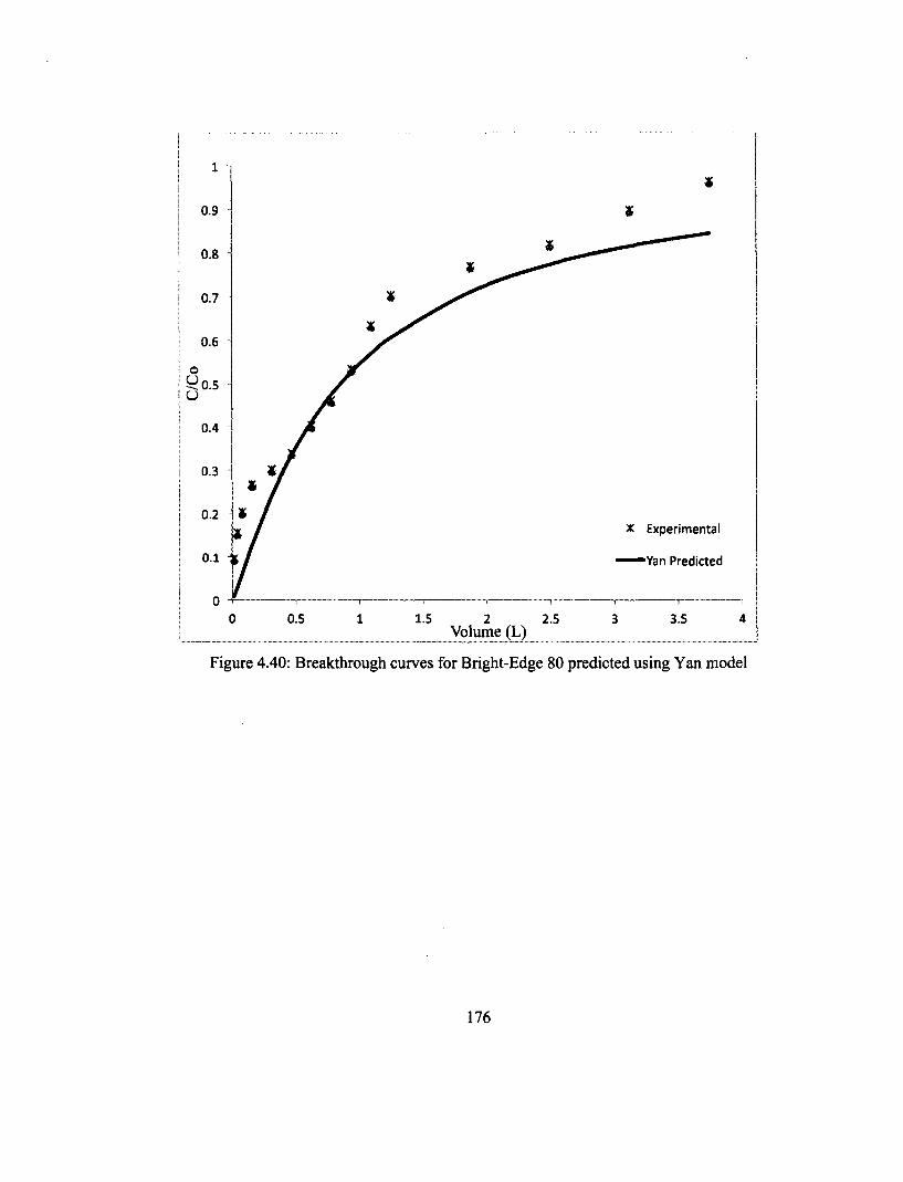
4
4
x Experimental
Yan Predicted
0 0.5 1 1.5 2 2.5 Volume (L)
Figure 4.40: Breakthrough curves for Bright-Edge 80 predicted using Yan model
176
3.5
0.9
0.8
0.7
0.6
0.4
0.3
0.2 * Experimental
0.1 Yan Predicted
0 0.5 4 1 1.5 2 2.5 3 3.5 Volume (L)
Figure 4.40: Breakthrough curves for Bright-Edge 80 predicted using Yan model
176

0.8
0 0.6
C.)
0
4 ............... ........
.....
-SMO C/CO Belter and Cussler Predicted
•-• SMO C/CO Chu 1 Predicted
SMO C/C0 Chu 2 Predicted
SMO C/CO Experimental
500 1000 1500
Time, min
2000 2500 3000
Figure 4.41: Breakthrough curves for SMO predicted using Belter and Chu models
177
0.8
SMO C/CO Belter and Cussler Predicted
0.4
SMO C/CO Chu 1 Predicted
SMO C/CO Chu 2 Predicted
0.2
* SMO C/CO Experimental
1000 3000 0 500 1500 2000 2500
Time, min
Figure 4.41: Breakthrough curves for SMO predicted using Belter and Chu models
177

X CO MO Experimental
CO MO Belter and Cussler Predicted
—• — CO MO Chu 1 Predicted
CO C/C0 Chu 2 Predicted
0 200 400 600 800 1000
Time, min
1200 1400 1600
Figure 4.42: Breakthrough curves for CO predicted using Better and Chu models
178
1
0.8
* CO C/CO Experimental 0.4
CO C/CO Belter and Cussler Predicted
CO C/CO Chu 1 Predicted 0.2
CO C/CO Chu 2 Predicted
0 200 600 0 400 1000 1200 1400 1600 800
Time, min
Figure 4.42: Breakthrough curves for CO predicted using Belter and Chu models
178
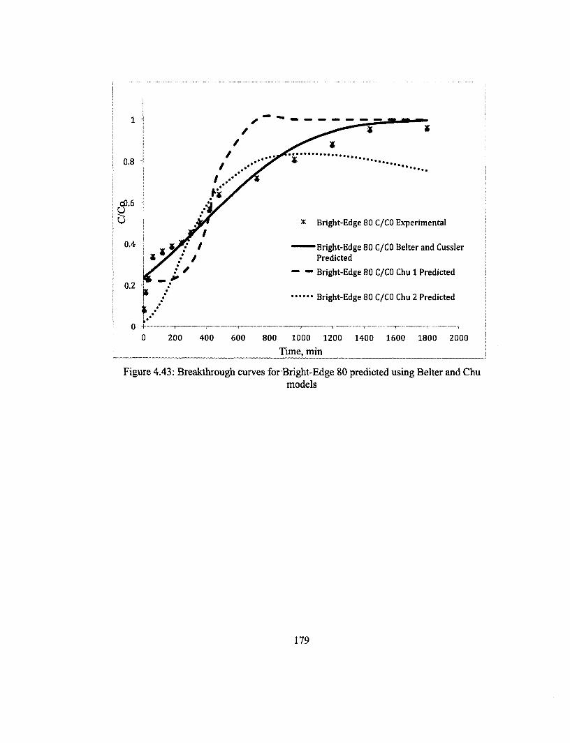
c0.6 frig
.1.1It WNW
4
.....
....................................
U Bright-Edge 80 C/CO Experimental
0.4 / """""•••"Bright-Edge 80 C/CO Belter and Cussler : Predicted
• ••• Bright-Edge 80 C/CO Chu 1 Predicted
0.2 Bright-Edge 80 C/CO Chu 2 Predicted
*•
1••••0 +
0 200 400 600 800 1000 1200 1400 1600 1800 2000
Time, min
Figure 4.43: Breakthrough curves for Bright-Edge 80 predicted using Belter and Chu models
179
0.8
* Bright-Edge 80 C/CO Experimental
0.4 Bright-Edge 80 C/CO Belter and Cussler
Predicted
Bright-Edge 80 C/CO Chu 1 Predicted
0.2 Bright-Edge 80 C/CO Chu 2 Predicted
0 200 400 600 800 1000 1200 1400 1600 1800 2000
Time, min
Figure 4.43: Breakthrough curves for Bright-Edge 80 predicted using Belter and Chu models
179
good fit to the model described by Equation 2.13 with r2 values higher than 0.92 at a 95%
confidence level. The model equation employed by Chu in Equation 2.15 (with negative
sign in exponential terms) fitted better than Equation 2.14 (with positive sign in
exponential terms) for all oils. In the case of SMO, the breakthrough curve was well
described by both Equations 2.13 and 2.15 showing a high r2 value (> 0.92) at a 95%
confidence interval. In the case of all oils, Equation 2.15 underestimates the effluent oil
concentration, while the model in Equation 2.14 overestimates the experimental values.
In addition, Equations 2.13 and 2.14 predict a nonzero effluent concentration at t = 0
which contradicts real conditions for the three oils. The modeling results of Chu (2004)
showed that Equation 2.14 was capable of simulating breakthrough curves with a broad
leading edge whileEquation 2.15 could be used to describe breakthrough curves with a
broad trailing edge. However, using these simple models to design or optimize fixed bed
biosorption columns requires knowledge of the effect of the process variables on the two
model parameters, to and a (Chu 2004).
4.15.4 The Yoon and Nelson Model
A simple theoretical model developed by Yoon—Nelson was applied to investigate the
breakthrough behavior of the oils on immobilized biomass beads. This model is based
upon the assumption that the rate of decrease in the probability of adsorption for each
adsorbate molecule is proportional to the probability of adsorbate adsorption and the
probability of adsorbate breakthrough on the adsorbent (Hamdaoui 2006). The values of
KyN and t12 are listed in Table 4.20. Breakthrough curves predicted using the Yoon and
180
good fit to the model described by Equation 2.13 with r2 values higher than 0.92 at a 95%
confidence level. The model equation employed by Chu in Equation 2.15 (with negative
sign in exponential terms) fitted better than Equation 2.14 (with positive sign in
exponential terms) for all oils. In the case of SMO, the breakthrough curve was well
described by both Equations 2.13 and 2.15 showing a high r2 value (> 0.92) at a 95%
confidence interval. In the case of all oils, Equation 2.15 underestimates the effluent oil
concentration, while the model in Equation 2.14 overestimates the experimental values.
In addition, Equations 2.13 and 2.14 predict a nonzero effluent concentration at t = 0
which contradicts real conditions for the three oils. The modeling results of Chu (2004)
showed that Equation 2.14 was capable of simulating breakthrough curves with a broad
leading edge whileEquation 2.15 could be used to describe breakthrough curves with a
broad trailing edge. However, using these simple models to design or optimize fixed bed
biosorption columns requires knowledge of the effect of the process variables on the two
model parameters, to and a (Chu 2004).
4.15.4 The Yoon and Nelson Model
A simple theoretical model developed by Yoon-Nelson was applied to investigate the
breakthrough behavior of the oils on immobilized biomass beads. This model is based
upon the assumption that the rate of decrease in the probability of adsorption for each
adsorbate molecule is proportional to the probability of adsorbate adsorption and the
probability of adsorbate breakthrough on the adsorbent (Hamdaoui 2006). The values of
Kyn and ti/2 are listed in Table 4.20. Breakthrough curves predicted using the Yoon and
180

Nelson model are given in Figures 4.44 — 4.46 for SMO, CO, and Bright-Edge 80,
respectively. Both CO and Bright-Edge 80 showed high correlation values (r > 0.95) and
the correlation was statistically significant (from t-test) at the 95% confidence level. The
model equations obtained with the non-linear regression analysis of the Yoon Nelson
model could describe the breakthrough data better for CO and Bright-Edge 80.
4.15.5 The Oulman Model
Experimental data were fitted to the Oulman model given in Equation 2.17
(Figures A.31 to A.33). Equation parameters such as K and No values are given in Table
4.20. The high correlation coefficient (r > 0.96) and the t statistical significance at the
95% confidence level indicated that the Oulman equation could describe the
breakthrough data reasonably. The Oulman equation, a re-written form of the Bohart—
Adams model can be considered a simple form of the Thomas model. When the isotherm
is highly favorable, the Thomas model is reduced to the Bohart—Adams. Bohart—Adams
model and is derived based on the assumption that adsorption is an irreversible second
order reaction. The rate constant K obtained from the Oulman model is approximately the
same as Kr , as predicted by the Thomas model.
4.15.6 The Wolborska Model
The Wolborska sorption model was applied to experimental data for the
description of the initial part of the breakthrough curve (Figures A.34 to A.36). This
approach was focused upon the estimation of characteristic parameters such as maximum
181
Nelson model are given in Figures 4.44 - 4.46 for SMO, CO, and Bright-Edge 80,
respectively. Both CO and Bright-Edge 80 showed high correlation values (r > 0.95) and
the correlation was statistically significant (from t-test) at the 95% confidence level. The
model equations obtained with the non-linear regression analysis of the Yoon Nelson
model could describe the breakthrough data better for CO and Bright-Edge 80.
4.15.5 The Oulman Model
Experimental data were fitted to the Oulman model given in Equation 2.17
(Figures A.31 to A.33). Equation parameters such as K and No values are given in Table
4.20. The high correlation coefficient (r > 0.96) and the t statistical significance at the
95% confidence level indicated that the Oulman equation could describe the
breakthrough data reasonably. The Oulman equation, a re-written form of the Bohart-
Adams model can be considered a simple form of the Thomas model. When the isotherm
is highly favorable, the Thomas model is reduced to the Bohart-Adams. Bohart-Adams
model and is derived based on the assumption that adsorption is an irreversible second
order reaction. The rate constant K obtained from the Oulman model is approximately the
same as Kt , as predicted by the Thomas model.
4.15.6 The Wolborska Model
The Wolborska sorption model was applied to experimental data for the
description of the initial part of the breakthrough curve (Figures A.34 to A.36). This
approach was focused upon the estimation of characteristic parameters such as maximum
181

0.9
0.8
0.7
0.6
9 .`-te. 0.5 • U
0.4
0.3
0.2 j 40.1 0.0
0 500 1000 1500 2000 2500 3000
Time (min)
Yoon Nelson Predicted
Experimental
Figure 4.44: Breakthrough curves for SMO predicted using Yoon and Nelson model
182
1.0
0.9
0.8
0.7
0.6
0.5
0.4
0.3
0.2 Yoon Nelson Predicted
* Experimental 0.1
0.0 500 1500 0 2500 1000 2000 3000
Time (min)
Figure 4.44: Breakthrough curves for SMO predicted using Yoon and Nelson model
182

1.0
0.9
0.8
0.7
0.3 4
0.2 4
0.1 -$
0.0 --0
4
200 400 600 800 1000
time (min)
Yoon Nelson Predicted
Experimental
1200 1400 1600
Figure 4.45: Breakthrough curves for CO predicted using Yoon and Nelson model
183
1.0
0.9
0.8
0.7
0.6
o ^ 0.5 O
0.4
0.3
Yoon Nelson Predicted 0.2
* Experimental 0.1
0.0 200 0 400 600 800 1000 1200 1400 1600
time (min)
Figure 4.45: Breakthrough curves for CO predicted using Yoon and Nelson model
183

1.0
0.9
0.8
0.7
0.6
0 Cz? 0.5
0.4
0.3
IS 0.2 i x ••••••••Yoon Nelson Predicted
0.1 x Experimental
0.0 4-- —/ , 0 200 400 600 800 1000 1200 1400 1600 1800 2000
Time (min)
Figure 4.46: Breakthrough curves for Bright-Edge 80 using Yoon and Nelson model
184
1.0
0.9
0.8
0.7
0.6
0.5
0.4
0.3
0.2 Yoon Nelson Predicted
0.1 * Experimental
0.0
0 200 400 600 800 1000 1200 1400 1600 1800 2000
Time (min) ^
Figure 4.46: Breakthrough curves for Bright-Edge 80 using Yoon and Nelson model
184

sorption capacity (No) and kinetic coefficient of the external mass transfer (pa). After
applying Equation 2.19 to the experimental data, a linear relationship between In (C/Co)
and t was obtained for In (C/Co) < —0.3, for all three breakthrough curves (r > 0.85).
Breakthrough curves for SMO and CO showed a high correlation coefficient (r > 0.9) at a
95% confidence interval. Respective values of No and pa calculated from the ln(C/Co)
versus t plots for the oils are presented in Table 4.20. This showed that the overall system
kinetics was dominated by external mass transfer in the initial part of sorption in the
column. The kinetic coefficient pa reflects the effect of both mass transfer in the liquid
phase and axial dispersion. Wolborska observed that in short beds or at high flow rates of
solution through the bed, the axial diffusion is negligible and 13a = Po, the external mass
transfer coefficient. Although the Wolborska model provides a simple and
comprehensive approach to running and evaluating sorption- column tests, its validity
was limited to the range of the used conditions. The expression of the Wolborska model
is equivalent to the Adams—Bohart relation if the coefficient KAB is equal to Pa /N0.
4.16 Column Regeneration and Reuse
Concentrations of oil in elutant for columns that had been fed SMO, CO, and
Bright-Edge 80, respectively are shown in Figures 4.47 — 4.49, respectively. The results
showed the adsorbed oils can be desorbed from the beads in the column. The desorption
produced no visible effects upon the physical properties of the beads. The re-generated
column was then fed with the same oil-in-water emulsion. The Thomas model equations
185
sorption capacity (No) and kinetic coefficient of the external mass transfer (pa). After
applying Equation 2.19 to the experimental data, a linear relationship between In (C/Co)
and t was obtained for In (C/Co) < -0.3, for all three breakthrough curves (r > 0.85).
Breakthrough curves for SMO and CO showed a high correlation coefficient (r > 0.9) at a
95% confidence interval. Respective values of No and pa calculated from the ln(C/Co)
versus t plots for the oils are presented in Table 4.20. This showed that the overall system
kinetics was dominated by external mass transfer in the initial part of sorption in the
column. The kinetic coefficient pa reflects the effect of both mass transfer in the liquid
phase and axial dispersion. Wolborska observed that in short beds or at high flow rates of
solution through the bed, the axial diffusion is negligible and Pa = p0) the external mass
transfer coefficient. Although the Wolborska model provides a simple and
comprehensive approach to running and evaluating sorption- column tests, its validity
was limited to the range of the used conditions. The expression of the Wolborska model
is equivalent to the Adams-Bohart relation if the coefficient KAB is equal to Pa /N0.
4.16 Column Regeneration and Reuse
Concentrations of oil in elutant for columns that had been fed SMO, CO, and
Bright-Edge 80, respectively are shown in Figures 4.47 - 4.49, respectively. The results
showed the adsorbed oils can be desorbed from the beads in the column. The desorption
produced no visible effects upon the physical properties of the beads. The re-generated
column was then fed with the same oil-in-water emulsion. The Thomas model equations
185

400 -
350
t 300
5 e 250 O • 200
6 • 150
(.5) 100 - 50
0
**
0 50 100 150 200 250 300 350 400 450 500
Time, min
Figure 4.47: Desorption profile for SMO using de-ionized water
186
400
350
300
„ 250 a o 13 200 -b a g 150 fi o u 100
50
0 0 50 100 150 200 250 300 350 400 450 500
Time, min
Figure 4.47: Desorption profile for SMO using de-ionized water
186

180
160
140
e 120
o 100
• 80
c.) O 60 0
40
20
0
•
•
• • # *
•
0 50 100 150 200 250 300 350
Time, min
Figure 4.48: Desorption profile for CO using de-ionized water
187
180 "
160 • , 140
"a. a 120
•
• o 100 t
1 80
a 60 -o U
40 •
20 •
N
0 0 50 100 150 200 250 300 350
Time, min
Figure 4.48: Desorption profile for CO using de-ionized water
187

Con
cent
rati
on,
160
140
120
100
80
60
40
20
0
•
50
* # #
100 150 200 250 300 350 400
Time, min
Figure 4.49: Desorption profile for Bright-Edge 80 using de-ionized water
188
160
140
120
100
80
60
40
20
0
•
50 100 150 200 250
Time, min
t * #
300 350 400
Figure 4.49: Desorption profile for Bright-Edge 80 using de-ionized water
188

and parameters kT and qo for the second run are shown in Table 4.20. The value of qo
obtained was 2.5, 0.03, and 0.5 mg/g for SMO, CO and Bright-Edge 80, respectively.
However, it may be noted that the correlation coefficient was much lower than that
obtained from the first cycle. Under the effluent pH and other similar operation
conditions, the qo value in the second cycle should not generally exceed the value in the
first cycle (Yan and Viraraghavan 2001). Nevertheless, it could be observed that the
regenerated beads retained the capability to adsorb oil. Figures 4.50 — 4.52 show the plot
of the ratio of effluent to influent oil concentration versus the bed volume for SMO, CO,
and Bright-Edge 80, respectively. As in the first cycle, the non-linear regression analysis
provided a higher correlation coefficient (r > 0.9) for all oils. Thus, based on the results, it
can be expected that the regenerated immobilized biomass can also be reused in a
biosorption column.
4.17 Coalescence/Filtration Mechanism
The head-loss across the immobilized biomass bed for single-phase flow was
predicted using Equation 2.20 and the linearized plot is presented in Figure 4.53. The plot
shows the pressure data fitted the equation very well, with an R2 value of 0.96. The
average value of the Carman-Kozeny constant (k1), determined from the slope of the
regression line, was 5.03. The value of k1, obtained for the immobilized M rouxii
biomass bed, appeared to be reasonable as similar k1 values were obtained by Carman
(1956) (4.5-5.1 for medium spheres) and Wiggins et al (1939) (4 to 6.5 for glass fibers,
189
and parameters kj and qo for the second run are shown in Table 4.20. The value of qo
obtained was 2.5, 0.03, and 0.5 mg/g for SMO, CO and Bright-Edge 80, respectively.
However, it may be noted that the correlation coefficient was much lower than that
obtained from the first cycle. Under the effluent pH and other similar operation
conditions, the qo value in the second cycle should not generally exceed the value in the
first cycle (Yan and Viraraghavan 2001). Nevertheless, it could be observed that the
regenerated beads retained the capability to adsorb oil. Figures 4.50 - 4.52 show the plot
of the ratio of effluent to influent oil concentration versus the bed volume for SMO, CO,
and Bright-Edge 80, respectively. As in the first cycle, the non-linear regression analysis
provided a higher correlation coefficient (r > 0.9) for all oils. Thus, based on the results, it
can be expected that the regenerated immobilized biomass can also be reused in a
biosorption column.
4.17 Coalescence/Filtration Mechanism
The head-loss across the immobilized biomass bed for single-phase flow was
predicted using Equation 2.20 and the linearized plot is presented in Figure 4.53. The plot
shows the pressure data fitted the equation very well, with an R2 value of 0.96. The
average value of the Carman-Kozeny constant (ki), determined from the slope of the
regression line, was 5.03. The value of ki, obtained for the immobilized M. rouxii
biomass bed, appeared to be reasonable as similar ki values were obtained by Carman
(1956) (4.5-5.1 for medium spheres) and Wiggins et al (1939) (4 to 6.5 for glass fibers,
189

1.2
4
0.8
U 0.
0.4 SMO C/Co - Experimental
0.2 —SMO C/Co - Thomas Predicted 4
0 0.5 1 1.5 2 2.5 3 3.5 4
Volume, L
Figure 4.50: Breakthrough curve for SMO for the second run
190
1.2
0.8
o
0.6 U
* SMO C/Co - Experimental 0.4
0.2 SMO C/Co - Thomas Predicted
0 0.5 1 1.5 2 2.5 3 3.5 4
Volume, L
Figure 4.50: Breakthrough curve for SMO for the second run
190

0 0.5
)1'. CO C/Co - Experimental
CO C/Co - Thomas Predicted
1 1.5
Volume, L
2
Figure 4.51: Breakthrough curve for CO for the second run
191
2.5
1.2
0.8
* CO C/Co - Experimental
0.4
CO C/Co - Thomas Predicted
0.2
0 0.5 1 1.5 2.5 2
Volume, L
Figure 4.51: Breakthrough curve for CO for the second run
191

1.2
0.8
0 U 0.6
0.4
0.2
0
Bright-Edge 80 C/Co - Experimental
Bright-Edge 80 C/Co - Thomas Predicted
0.5 1 1.5 2 2.5 3
Volume, L
Figure 4.52: Breakthrough curve for Bright-Edge 80 for the second run
192
1.2
1
0.8
* Bright-Edge 80 C/Co - Experimental 0.6
0.4
Bright-Edge 80 C/Co - Thomas
Predicted 0.2
0 0.5 1.5 2.5 0 1 2 3
Volume, L
Figure 4.52: Breakthrough curve for Bright-Edge 80 for the second run
192

0.35
0.3
0.25
0.1 1
0.05
0 4-
0 0.01 0.02 0.03 0.04 0.05 0.06 0.07
y = 5.03x - 0.02 R2 =0.96
36uy,(1-E)2/(df2gcE3)
Figure 4.53: Linearized plot of single-phase flow pressure drop
193
0.05
0
y = 5.03x- 0.02
R2 = 0.96
0 0.01 0.02 0.03 0.04 0.05 0.06 0.07
36UYc(l-£)V(df2gcE3)
Figure 4.53: Linearized plot of single-phase flow pressure drop
193
glass wool, fiber glass and yarn). The condition of laminar flow defined by Equation 2.23
with Reynolds numbers of 1.6 to 4.3 and a porosity value of 0.475 was valid. A summary
of coalescence/filtration performance and the values of k1, as reported in literature, are
shown in Table 4.22. The specific permeability coefficient (Bo) of the immobilized
biomass beads, calculated using Equation 2.23 with a k1 value of 5.03, was found to be
-8 2 2.135 x 10 m . The value of Tortuosity (T) for immobilized biomass medium with a
porosity of 0.475 was found to be 2.105. Using the value of T in Equation 2.22, the value
of ko (shape factor) was calculated as 1.13. Carman (1956) reported the ko value to be in
the range of 1.2 to 3.0 depending upon the media shape. Moazed and Viraraghavan
(2002) observed a low T value of 1.0 for an organo-clay/anthracite mixture used in their
study and attributed that it may be due to the characteristics of the mixed media. The
filtration model of Carman-Kozeny for single-phase flow, as given by Equation 2.20, was
used to predict the head-loss across the immobilized M rouxii biomass bed at different
depths. The results of the predicted and experimental head-losses across the bed for
single-phase flow (Regina tap water) are shown in Figure 4.54. The high correlation
coefficient with a R2 value of 0.99 indicated that the Carman-Kozeny filtration model can
be applied to predict the head-loss from the single-phase flow through the immobilized
M rouxii biomass bed. The data of pressure drop from the two-phase (oil-in-water
emulsion) flow through the immobilized M rouxii biomass bed was analyzed using
Equation 2.21 to evaluate the Carman-Kozeny constant, k2. The linear plot of Equation
2.21 for two-phase flow is shown in Figure 4.55. The results of predicted and
experimental head-losses across the bed for two-phase flow are shown in Figure 4.56. A
194
glass wool, fiber glass and yarn). The condition of laminar flow defined by Equation 2.23
with Reynolds numbers of 1.6 to 4.3 and a porosity value of 0.475 was valid. A summary
of coalescence/filtration performance and the values of ki, as reported in literature, are
shown in Table 4.22. The specific permeability coefficient (Bo) of the immobilized
biomass beads, calculated using Equation 2.23 with a kj value of 5.03, was found to be
-8 2
2.135 x 10 m . The value of Tortuosity (T) for immobilized biomass medium with a
porosity of 0.475 was found to be 2.105. Using the value of T in Equation 2.22, the value
of ko (shape factor) was calculated as 1.13. Carman (1956) reported the ko value to be in
the range of 1.2 to 3.0 depending upon the media shape. Moazed and Viraraghavan
(2002) observed a low T value of 1.0 for an organo-clay/anthracite mixture used in their
study and attributed that it may be due to the characteristics of the mixed media. The
filtration model of Carman-Kozeny for single-phase flow, as given by Equation 2.20, was
used to predict the head-loss across the immobilized M. rouxii biomass bed at different
depths. The results of the predicted and experimental head-losses across the bed for
single-phase flow (Regina tap water) are shown in Figure 4.54. The high correlation
coefficient with a R2 value of 0.99 indicated that the Carman-Kozeny filtration model can
be applied to predict the head-loss from the single-phase flow through the immobilized
M. rouxii biomass bed. The data of pressure drop from the two-phase (oil-in-water
emulsion) flow through the immobilized M. rouxii biomass bed was analyzed using
Equation 2.21 to evaluate the Carman-Kozeny constant, k.2. The linear plot of Equation
2.21 for two-phase flow is shown in Figure 4.55. The results of predicted and
experimental head-losses across the bed for two-phase flow are shown in Figure 4.56. A
194

Table 4.22: Summary of coalescence and filtration data
Influent characteristics
Media characteristics
Design factors
Final oil concen-tration
K1 Reference
•
Lab-prepared Fibrous glass Filter area 30 ppm 4.4 Chieu et al. emulsified coker #2 oil, 100 ppm
material, 10 mm fiber size, 75% porosity
0.018 m2, loading rate 5 m3
m2/day
(1975)
Lab-prepared Horticultural Filter area 79 126 — 3.4 Mathavan and emulsified peat, 1.6 mm cm2
, loading 130 Viraraghavan mineral oil in water, 131 mg/L
particle dia, 79% porosity
rate 0.26 — 0.51 m3
m2/day
mg/L (1992)
Lab-prepared Organo- Filter area 2.8 45 — 46 4.29 Moazed and emulsified clay/anthracite cm2, loading mg/L Viraraghavan mineral oil in water, 48 mg/L
mixture, 2.1 mm particle dia, 48.5% porosity
rate 1 — 2.7 gpm/ft2
(2002)
Lab-prepared Polypropylene 254 — 581 12.8 Li and Gu emulsified instow crude oil/ mineral oil in water, 2000, 5000 and 10000 ppm
fibres, 170 gm, 48% porosity
Nylon fibres, 80
'1111, 45%
porosity
mL/min
.367 — 813 mL/min
(2005)
Granular polypropylene, 684 iirn, porosity 38.4%
177 — 542 mL/min
9.67
Produced water 1 - 264
Granular media, 0.569 mm
Filter area 5.5 cm2, 2 — 10
13.3 — 23.2
1.5 Multon and Viraraghavan
mg/L
Produced water 2 — 212 mg/L
particle size, 56% porosity
gpm/ft2 mg/L
7.1 — 56.8 mg/L
(2006)
Lab-prepared Immobilized M Filter area 2.8 47 — 48 5.03 Present study emulsified mineral oil in water, 50 mg/L
rouxii, 2.11 mm particle dia, 47.5% porosity
cm2, loading rate 1 — 2.7 gpm/ft2
mg/L
195
Table 4.22: Sximmary of coalescence and filtration data
Influent characteristics
Media characteristics
Design factors
Final oil concentration
K, Reference
Lab-prepared emulsified coker #2 oil, 100 ppm
Fibrous glass material, 10 mm fiber size, 75% porosity
Filter area 0.018 m2, loading rate 5 m3 m2/day
30 ppm 4.4 Chieu et al. (1975)
Lab-prepared emulsified mineral oil in water, 131 mg/L
Horticultural peat, 1.6 mm particle dia, 79% porosity
Filter area 79 cm2, loading rate 0.26 -0.51 m3
m2/day
126 -130 mg/L
3.4 Mathavan and Viraraghavan (1992)
Lab-prepared emulsified mineral oil in water, 48 mg/L
Organo-clay/anthracite mixture, 2.1 mm particle dia, 48.5% porosity
Filter area 2.8 cm2, loading rate 1 - 2.7 gpm/ft2
45 -46 mg/L
4.29 Moazed and Viraraghavan (2002)
Lab-prepared emulsified instow crude oil/ mineral oil in water, 2000, 5000 and 10000 ppm
Polypropylene fibres, 170 [im, 48% porosity
Nylon fibres, 80 Hm, 45% porosity
Granular polypropylene, 684 nm, porosity 38.4%
254 - 581 mL/min
•367 - 813 mL/min
177 - 542 mL/min
12.8
9.67
Li and Gu (2005)
Produced water 1 - 264 mg/L
Produced water 2 - 212 mg/L
Granular media, 0.569 mm particle size, 56% porosity
Filter area 5.5 c m 2 , 2 - 1 0 gpm/ft2
13.3 -23.2 mg/L
7.1 -56.8 mg/L
1.5 Multon and Viraraghavan (2006)
Lab-prepared emulsified mineral oil in water, 50 mg/L
Immobilized M. rouxii, 2.11 mm particle dia, 47.5% porosity
Filter area 2.8 •y
cm, load ing rate 1 - 2.7 gpm/ft2
47-48 mg/L
5.03 Present study
195

0.35
0.3 -
a..3
0.25
0.2
0.15 -
6' 0 1a. •
0.05
0 0 0.05 0.1 0.15 0.2
Experimental APJL
y 1.09x + 0.0004 R2 =0.99
- - • - 45 degree line
Linear (Trendline)
0.25
Figure 4.54: Predicted versus actual headloss for single-phase flow
196
0.3
•
0.35
0.3
>0.25 Qm | 0.2
2 0.15 13 t 01
0.05
0
y = 1.09x + 0.0004 R2 = 0.99
0.05 0.1 0.15 0.2
Experimental AP/L
45 degree line
Linear (Trendline)
0.25 0.3
Figure 4.54: Predicted versus actual headloss for single-phase flow
196

0.9 -
0.8 -
0.7 -
0.6
0.5 -a <3 0.4 -
0.3 -
0.2
0.1 -
0
y = 2.98x + 0.04 R2 =0.86 vAk
•
0 0.02 0.04 0.06 0.08 0.1 0.12 0.14 0.16 0.18
3611,4:(1-02/(d?g,f t3)
Figure 4.55: Linearized plot of two-phase flow pressure drop
197
0.9
0.8
0.7
0.6
< 0.5 h <1 0.4
0.3
0.2
0.1
0
y = 2.98x + 0.04
R2 = 0.86
0.02 0.04 0.06 0.08 0.1 0.12
36Uyc(l-hy/(d(%^)
0.14 0.16 0.18
Figure 4.55: Linearized plot of two-phase flow pressure drop
197

0.6
0.5
0.4
,E•1 0.3 Q
"CJ 2
41" 0.2
0.1
0
♦ *
y = 1.05x - 0.03 R2 = 0.97 •
- • - • - 45 degree line
0.05 0.1 0.15 0.2 0.25 0.3
Experimental AWL
0.35
Linear (Trendline)
r
0.4 0.45 0.5
Figure 4.56: Predicted versus actual headloss for single-phase flow
198
0.6
y = 1.05x - 0.03
R2 = 0.97
45 degree line 0.2
Linear
(Trendline)
—r—
0.1
—r
0.2
~f~~ """ '"T 0.25 0.3
-p. ..
0.35
""" T "'"T 0.4 0.45 0 0.05 0.15 0.5
Experimental AP/L
Figure 4.56: Predicted versus actual headloss for single-phase flow
198

high correlation coefficient with a R2 value of 0.97 was obtained. The average value of k2,
as determined from the slope of the regression line was 2.98. In general, as far as the two-
phase flow, the head-loss predictions were closer to the measured values at lower flow
rates. As for higher flow rates, especially in the case of two-phase flow, the predicted
head-loss values were higher than the measured values at all depths of the bed. A similar
trend has been found both by Mathavan and Viraraghavan (1992) and Moazed and
Viraraghavan (2002) and the difference was attributed to be between predicted and
measured head-loss values to differences in average saturation for various flow rates.
The specific permeability coefficient (Bo) obtained for two-phase flow, using Equation
-8 2 2.23, was found to be 1.58 x 10 m . The permeability coefficient for two-phase flow did
not differ appreciably compared with the single-phase flow permeability. Both Mathavan
and Viraraghavan (1992) and Moazed and Viraraghavan (2002) observed a slight
decrease in permeability for two-phase flow due to the negligible void space occupied by
the oil droplets in the bed. The average saturation (SO was calculated using Equation
2.26. Table 4.23 provides average saturation values for the immobilized M rouxii
biomass bead bed used in this study. The degree of saturation was found to increase with
an increasing flow rate. Average saturations of 10.3% and 20.8% were obtained for flow
rates of 12 mL/min and 32 mL/min, respectively. The overall coalescence efficiency (Tic)
was calculated using Equation 2.25 for each flow rate. Results are given in Table 4.24. A
plot of coalescence efficiency versus Reynolds number for different bed depths is given
in Figure 4.57. The coalescence efficiency is plotted against Reynolds number to ensure
199
high correlation coefficient with a R2 value of 0.97 was obtained. The average value of k2,
as determined from the slope of the regression line was 2.98. In general, as far as the two-
phase flow, the head-loss predictions were closer to the measured values at lower flow
rates. As for higher flow rates, especially in the case of two-phase flow, the predicted
head-loss values were higher than the measured values at all depths of the bed. A similar
trend has been found both by Mathavan and Viraraghavan (1992) and Moazed and
Viraraghavan (2002) and the difference was attributed to be between predicted and
measured head-loss values to differences in average saturation for various flow rates.
The specific permeability coefficient (Bo) obtained for two-phase flow, using Equation
-8 2
2.23, was found to be 1.58 * 10 m . The permeability coefficient for two-phase flow did
not differ appreciably compared with the single-phase flow permeability. Both Mathavan
and Viraraghavan (1992) and Moazed and Viraraghavan (2002) observed a slight
decrease in permeability for two-phase flow due to the negligible void space occupied by
the oil droplets in the bed. The average saturation (Sd) was calculated using Equation
2.26. Table 4.23 provides average saturation values for the immobilized M. rouxii
biomass bead bed used in this study. The degree of saturation was found to increase with
an increasing flow rate. Average saturations of 10.3% and 20.8% were obtained for flow
rates of 12 mL/min and 32 mL/min, respectively. The overall coalescence efficiency (r]c)
was calculated using Equation 2.25 for each flow rate. Results are given in Table 4.24. A
plot of coalescence efficiency versus Reynolds number for different bed depths is given
in Figure 4.57. The coalescence efficiency is plotted against Reynolds number to ensure
199

Table 4.23: Average saturation values of the immobilized M rouxii biomass bed
Flow (mL/min) A P1 A P2 A P1/is P2 B Et Sd
12 0.098 0.162 0.605 0.235 0.426 0.103
16 0.125 0.219 0.568 0.198 0.41 0.137
20 0.156 0.281 0.557 0.167 0.395 0.169
24 0.201 0.332 0.609 0.157 0.388 0.182
28 0.230 0.392 0.589 0.144 0.381 0.198
32 0.276 0.454 0.613 0.136 0.376 0.208
200
Table 4.23: Average saturation values of the immobilized M. rouxii biomass bed
Flow (mL/min) API A P2 AP1/AP2 B sd
12 0.098 0.162 0.605 0.235 0.426 0.103
16 0.125 0.219 0.568 0.198 0.41 0.137
20 0.156 0.281 0.557 0.167 0.395 0.169
24 0.201 0.332 0.609 0.157 0.388 0.182
28 0.230 0.392 0.589 0.144 0.381 0.198
32 0.276 0.454 0.613 0.136 0.376 0.208
200

Table 4.24: Coalescence efficiency
Coalescence efficiency (fraction)
Bed height (mm) Flow rate (mL/min)
12 16 20 24 28 32
20 0.159 0.12 0.10 0.081 0.080 0.080
40 0.086 0.067 0.054 0.053 0.047 0.047
60 0.060 0.048 0.039 0.039 0.035 0.032
80 0.045 0.039 0.028 0.032 0.027 0.026
100 0.041 0.034 0.027 0.025 0.023 0.020
201

0200 mm 0.18 —
❑400 mm ›, 0.16 -
A600 mm -6 0.14
T)X800 mm
0.12
8 ce) a)
0.1
0.08 0 0 0
X1000 mm
U 0.06
0.04 U
0.02
0 0 0.1 0.2 0.3
log NRe
0.4 0.5 0.6
Figure 4.57: Coalescence efficiency versus Reynolds number
202
0.18
>> 0.16 o c 0) 0.14
0.12
o B o u ca 8 o.i CO <D K 0-08 o
0.06
0.04
0.02
0
0
•
6 0
A 1
•
0200 mm
• 400 mm
A 600 mm
X800 mm
*1000 mm
0 0 0
• •
0.1 0.2 0.3 0.4 0.5 0.6
log NRe
Figure 4.57: Coalescence efficiency versus Reynolds number
202

laminar flow in the system. In the laminar flow regime, the oil droplets will be considered
as moving in streamlines and wall effects will become negligible. The coalescence
efficiency was a maximum for the flow rate of 12 mL/min at all depths. The overall
coalescence efficiency ranged from 15.9 to 4% at the lowest flow rate of 12 mL/min and
from 8 to 2% at the highest flow rate of 32 mL/min. It is possible that a flow rate of 12
mL/min might be the optimum velocity to attain maximum coalescence efficiency in the
immobilized M rouxii biomass bed. However, Sherony et al. (1978) observed an increase
in coalescence efficiency with increasing velocity. Yet, it was pointed out that Sherony's
filtration theories were not very successful at predicting the capture of particulates from
water by sand beds, likely due to the underestimation of surface chemical forces in the
filtration theory (Speilman and Goren 1970). The coalescence efficiency was observed to
decrease with an increase in bed depth. Maximum and minimum coalescence efficiencies
of 15.9% and 4.0% were obtained at 200 mm and 1000 mm depth, respectively for a flow
rate of 12 mL/min. Both Mathavan and Viraraghavan (1992) and Moazed and
Viraraghavan (2002) who conducted similar studies on SMO observed decreasing
efficiency with an increasing bed depth. However, this contradicts the findings of
Sherony et al. (1971b) where the efficiency was found to increase with depth. Chieu et al.
(1975) predicted that a minimum oil saturation of 10 to 15% was necessary for
coalescence to occur in a synthetic media. In the present study, the saturation values
ranged from 10 to 20%. However, the low coalescence efficiency obtained could be
attributed to high stability of the SMO emulsion that was stabilized using emulsifiers in
the study. Mathavan and Viraraghavan (1992) concluded the peat bed used in their study
203
laminar flow in the system. In the laminar flow regime, the oil droplets will be considered
as moving in streamlines and wall effects will become negligible. The coalescence
efficiency was a maximum for the flow rate of 12 mL/min at all depths. The overall
coalescence efficiency ranged from 15.9 to 4% at the lowest flow rate of 12 mL/min and
from 8 to 2% at the highest flow rate of 32 mL/min. It is possible that a flow rate of 12
mL/min might be the optimum velocity to attain maximum coalescence efficiency in the
immobilized M. rouxii biomass bed. However, Sherony et al. (1978) observed an increase
in coalescence efficiency with increasing velocity. Yet, it was pointed out that Sherony's
filtration theories were not very successful at predicting the capture of particulates from
water by sand beds, likely due to the underestimation of surface chemical forces in the
filtration theory (Speilman and Goren 1970). The coalescence efficiency was observed to
decrease with an increase in bed depth. Maximum and minimum coalescence efficiencies
of 15.9% and 4.0% were obtained at 200 mm and 1000 mm depth, respectively for a flow
rate of 12 mL/min. Both Mathavan and Viraraghavan (1992) and Moazed and
Viraraghavan (2002) who conducted similar studies on SMO observed decreasing
efficiency with an increasing bed depth. However, this contradicts the findings of
Sherony et al. (1971b) where the efficiency was found to increase with depth. Chieu et al.
(1975) predicted that a minimum oil saturation of 10 to 15% was necessary for
coalescence to occur in a synthetic media. In the present study, the saturation values
ranged from 10 to 20%. However, the low coalescence efficiency obtained could be
attributed to high stability of the SMO emulsion that was stabilized using emulsifiers in
the study. Mathavan and Viraraghavan (1992) concluded the peat bed used in their study
203

could not filter or coalesce highly stable emulsions having droplet diameters of less than
10 gm. In the present study, droplet diameters of less than 6.9 gm were not found and the
results may agree with the findings of Mathavan and Viraraghavan (1992). The plot of
the ratio of drop diameter to immobilized M rouxii biomass bead diameter for various
flow rates at various depths is given in Figure 4.58. In the study, the initial average drop
diameter of the oil droplet was measured to be 21 gm and as the experiments proceeded,
the diameter of the oil droplets was lower than approximately 12.5 gm (range 6.9 — 12. 5
gm) at the end of the runs. The ratio of the drop diameter to biomass bead diameter
decreased as the bed depth increased from 200 mm to 1000 mm for all flow rates. The
ratio followed a decreasing trend with the bed depth for all flow rates. This decrease in
the ratio can be attributed to the filtration of drops with the biomass bed depth. The
influent drop diameter was 21 gm while the drop diameter of the effluent was less than
12.5 p.M. The decrease in the drop diameter in the effluent could be due to larger droplets
being filtered out and smaller droplets coalescing to form particles that are large enough
to be filtered out. The average holdup of the immobilized M rouxii biomass bed was
calculated using Equation 2.28. The plot of average holdup versus Reynolds number is
given in Figure 4.59. The holdup equation showed a fair agreement with experimental
data. The average holdup values of the bed increased as the Reynolds number increased.
However, Sherony et al. (1978) observed a decreasing bed holdup with an increasing
Reynolds number. It should be noted that the Reynolds numbers in their study were in the
range of 0.1 —1.0 in comparison to Reynolds numbers found in the present study (1.49 to
204
could not filter or coalesce highly stable emulsions having droplet diameters of less than
10 Jim. In the present study, droplet diameters of less than 6.9 jim were not found and the
results may agree with the findings of Mathavan and Viraraghavan (1992). The plot of
the ratio of drop diameter to immobilized M. rouxii biomass bead diameter for various
flow rates at various depths is given in Figure 4.58. In the study, the initial average drop
diameter of the oil droplet was measured to be 21 urn and as the experiments proceeded,
the diameter of the oil droplets was lower than approximately 12.5 (im (range 6.9 - 12. 5
(Am) at the end of the runs. The ratio of the drop diameter to biomass bead diameter
decreased as the bed depth increased from 200 mm to 1000 mm for all flow rates. The
ratio followed a decreasing trend with the bed depth for all flow rates. This decrease in
the ratio can be attributed to the filtration of drops with the biomass bed depth. The
influent drop diameter was 21 nm while the drop diameter of the effluent was less than
12.5 (Am. The decrease in the drop diameter in the effluent could be due to larger droplets
being filtered out and smaller droplets coalescing to form particles that are large enough
to be filtered out. The average holdup of the immobilized M. rouxii biomass bed was
calculated using Equation 2.28. The plot of average holdup versus Reynolds number is
given in Figure 4.59. The holdup equation showed a fair agreement with experimental
data. The average holdup values of the bed increased as the Reynolds number increased.
However, Sherony et al. (1978) observed a decreasing bed holdup with an increasing
Reynolds number. It should be noted that the Reynolds numbers in their study were in the
range of 0.1 - 1.0 in comparison to Reynolds numbers found in the present study (1.49 to
204

0.065 012 mL/min ❑16 mL/min
20 mL/min X24 mL/min
0.06 X28 mL/min 032 mL/min
0.055 - 0 b
7:1
0.05
0 0 A
0.045
0.04 0 20 40 60 80 100
Bed height, mm
Figure 4.58: Plot of the ratio of the drop diameter to the immobilized M rouxii biomass bead diameter versus bed depth for various flow rates
205
0.065
0.06
0.055
T3 ^5 TJ
0.05
0.045
0.04
• 0 6
20
& • 0
012 mL/min • 16 mL/min
A20 mL/min X24 mL/min
*28 mL/min 032 mL/min
0
B y
0
&
40 60
Bed height, mm
0
A
80
6
100
Figure 4.58: Plot of the ratio of the drop diameter to the immobilized M. rouxii biomass bead diameter versus bed depth for various flow rates
205

0.14
0.12
♦ 0.1 - y = 0.13x + 0.058
R2 =0.97
0,, 0.08 ♦
0 0.06
0.04 -
0.02 -
0 0 0.1 0.2 0.3 0.4 0.5 0.6
log NRe
Figure 4.59: Average holdup versus Reynolds number
206
y = 0.13x +0.058
0 0.1 0.2 0.3 0.4 0.5 0.6
log NRe
Figure 4.59: Average holdup versus Reynolds number
206

3.65). A decrease in coalescence efficiency, effluent oil concentration and effluent drop
diameter can all be attributed to the action of filtration and coalescence. Equations 2.29
and 2.30 were applied to the coalescence data to evaluate the model proposed by
Crickmore et al. (1989). The simplistic empirical model describes coalescence as a first
order rate equation. Influent and effluent oil concentrations were used in the equation as
the fraction of the fluid emulsified at the entrance and exit to the packed bed (Multon and
Viraraghavan 2006). ln(CA/CAO) versus t' was plotted to determine the rate constants for
coalescence (Figure 4.60). The coalescence data for SMO fitted the Crickmore model
reasonably well (R2 = 0.93). Rate constant (1c) from the plot was determined to be
0.0011 cm2/h. The value of the rate constant in this study appeared to be low compared to
the range of values obtained by Crickmore et al. (1989) (0.021 to 0.056 cm2/s) and
Multon and Viraraghavan (2006) (0.0032 and 0.0143 cm2/min). Additional experimental
runs with different bed depths, as carried out by Crickmore et al. (1989), may be required
to evaluate the suitability of this model in order to predict coalescence kinetics. Due to
the simplicity of this equation, it was difficult to determine whether it models
coalescence, filtration, or a combination of both (Multon and Viraraghavan 2006).
207
3.65). A decrease in coalescence efficiency, effluent oil concentration and effluent drop
diameter can all be attributed to the action of filtration and coalescence. Equations 2.29
and 2.30 were applied to the coalescence data to evaluate the model proposed by
Crickmore et al. (1989). The simplistic empirical model describes coalescence as a first
order rate equation. Influent and effluent oil concentrations were used in the equation as
the fraction of the fluid emulsified at the entrance and exit to the packed bed (Multon and
Viraraghavan 2006). ln(CA/CAO) versus T' was plotted to determine the rate constants for
coalescence (Figure 4.60). The coalescence data for SMO fitted the Crickmore model
reasonably well (R2 = 0.93). Rate constant (Kc) from the plot was determined to be
0.0011 cm2/h. The value of the rate constant in this study appeared to be low compared to
the range of values obtained by Crickmore et al. (1989) (0.021 to 0.056 cm2/s) and
Multon and Viraraghavan (2006) (0.0032 and 0.0143 cm2/min). Additional experimental
runs with different bed depths, as carried out by Crickmore et al. (1989), may be required
to evaluate the suitability of this model in order to predict coalescence kinetics. Due to
the simplicity of this equation, it was difficult to determine whether it models
coalescence, filtration, or a combination of both (Multon and Viraraghavan 2006).
207

1 rr- 1
10 20 30 40 50 60 70 80 90 100
-0.02
-0.04
-0.06 u
-0.0s
-0.1
-0.12
-0.14 hfcm2
y = -0.0011x - 0.022 Rz = 0.93
Figure 4.60: Coalescence kinetics for SMO predicted by the Crickmore model
208
0 0 I ( I f I J 1 I 1
1 10 20 30 40 50 60 70 80 90 100
-0.02 - y =-0.001 lx-0.022 Rz = 0.93
-0.04 "
§-0.06 " y • u 5 - 0 0 8 -
-0.1
-0.12 • -0.14 ^ -0.14 ^
t', h/cm2
Figure 4.60: Coalescence kinetics for SMO predicted by the Crickmore model
208
Chapter 5
Conclusion and Recommendations
5.1 Conclusion
The potential of fungus M rouxii to remove three different oils from water was
investigated via a series of batch and dynamic column studies. The following summations
were drawn based on the studies:
1. The factorial design of the experiments showed the pH was the most influential
parameter with respect to the removal of SMO, CO and Bright-Edge 80 by M
rouxii biomass. Adsorbent dose and temperature were found to have an effect on
the removal of SMO, oil concentration had an effect on the removal of CO and
temperature was found to have an effect on the removal of Bright-Edge 80. It is
important to note that these statements are valid within the lower and upper limits
of the factors: adsorbent dose (0.05 g to 0.5 g), temperature (5 to 30°C),
concentration (50 to 350 mg/L) and speed (100 to 200 rpm).
2. The results of batch adsorption studies showed M rouxii biomass could remove
up to 98% of oil from water. A decrease in the pH of solution led to a significant
increase in the oil-sorption capacity of the biomass. Adsorption of the three oils
was best at pH 3.0, the zero point charge of the biomass. Oil sorption on M rouxii
biomass was rapid with an equilibrium time of less than 3 hours. The rate of
adsorption of the three oils onto the M rouxii biomass was initially fast, followed
by a second phase characterized by slow sorption. Temperature had a relatively
minor effect as adsorption capacities of the biomass.
209
Chapter 5
Conclusion and Recommendations
5.1 Conclusion
The potential of fungus M. rouxii to remove three different oils from water was
investigated via a series of batch and dynamic column studies. The following summations
were drawn based on the studies:
1. The factorial design of the experiments showed the pH was the most influential
parameter with respect to the removal of SMO, CO and Bright-Edge 80 by M.
rouxii biomass. Adsorbent dose and temperature were found to have an effect on
the removal of SMO, oil concentration had an effect on the removal of CO and
temperature was found to have an effect on the removal of Bright-Edge 80. It is
important to note that these statements are valid within the lower and upper limits
of the factors: adsorbent dose (0.05 g to 0.5 g), temperature (5 to 30°C),
concentration (50 to 350 mg/L) and speed (100 to 200 rpm).
2. The results of batch adsorption studies showed M. rouxii biomass could remove
up to 98% of oil from water. A decrease in the pH of solution led to a significant
increase in the oil-sorption capacity of the biomass. Adsorption of the three oils
was best at pH 3.0, the zero point charge of the biomass. Oil sorption on M. rouxii
biomass was rapid with an equilibrium time of less than 3 hours. The rate of
adsorption of the three oils onto the M. rouxii biomass was initially fast, followed
by a second phase characterized by slow sorption. Temperature had a relatively
minor effect as adsorption capacities of the biomass.
209

3. Adsorption process was found to follow the pseudo second-order model. An
analysis of data showed that an infra-particle diffusion mechanism could play a
significant role in adsorption of oil by the biomass, and it was likely that
adsorption rate was controlled by a diffusion process.
4. The equilibrium data for the tested three oils were adequately described by the
Langmuir and Freundlich isotherm models. The oil sorption process was found to
be spontaneous and endothermic. Carboxyl and amide functional groups in the
biomass were likely involved in oil biosorption.
5. The Wolborska model better described the initial part of the breakthrough curve.
The Belter model reasonably predicted the experimental data. The breakthrough
curves were not described well by the modified Chu model equations. The
simulation of the whole breakthrough curve was better reflected by the Thomas,
Yan and Yoon Nelson models.
6. Both single-phase and two-phase flow data were shown to fit the Carman-Kozeny
equation. Average saturation values of the immobilized M rouxii biomass,
obtained from the Carman-Kozeny equation, increased with an increasing flow
rate. Maximum and minimum coalescence efficiencies of 15.9% and 4.0% were
obtained at 200 mm and 1000 mm depth, respectively, for a flow rate of 12
mL/min. The Crickmore model was adequate to describe the
coalescence/filtration of an oil-in-water emulsion as a first order rate equation.
210
3. Adsorption process was found to follow the pseudo second-order model. An
analysis of data showed that an intra-particle diffusion mechanism could play a
significant role in adsorption of oil by the biomass, and it was likely that
adsorption rate was controlled by a diffusion process.
4. The equilibrium data for the tested three oils were adequately described by the
Langmuir and Freundlich isotherm models. The oil sorption process was found to
be spontaneous and endothermic. Carboxyl and amide functional groups in the
biomass were likely involved in oil biosorption.
5. The Wolborska model better described the initial part of the breakthrough curve.
The Belter model reasonably predicted the experimental data. The breakthrough
curves were not described well by the modified Chu model equations. The
simulation of the whole breakthrough curve was better reflected by the Thomas,
Yan and Yoon Nelson models.
6. Both single-phase and two-phase flow data were shown to fit the Carman-Kozeny
equation. Average saturation values of the immobilized M. rouxii biomass,
obtained from the Carman-Kozeny equation, increased with an increasing flow
rate. Maximum and minimum coalescence efficiencies of 15.9% and 4.0% were
obtained at 200 mm and 1000 mm depth, respectively, for a flow rate of 12
mL/min. The Crickmore model was adequate to describe the
coalescence/filtration of an oil-in-water emulsion as a first order rate equation.
210

5.2 Practical Research Applications
By using the maximum adsorption capacity data of an adsorbent for the particular
oil-in-water emulsion, it is possible to calculate the amount of adsorbent required to
reduce oil in oily water to a desired concentration. The amount and cost of different
biomaterials used in the preliminary study, as required to obtain an effluent concentration
of 10 mg/L for SMO for a daily flow of 100 m3/d, are shown in Table 5.1. The amount of
powdered M rouxii biomass required to reduce oil from water to a desired concentration
can be determined by applying the relevant adsorption isotherm (Table 5.2). Batch
adsorption systems, which are basically operated on a fill-and-draw basis, are suitable to
treat small wastewater volumes. The CCRL, Regina, Saskatchewan, Canada treats
approximately 4700 m3/d of effluent with an average initial oil concentration of 350
mg/L and the treated effluent has an average oil concentration of 10-15 mg/L. The
wastewater treatment plant at the CCRL includes an American Petroleum Institute (API)
separator followed by an equalization pond, two aeration ponds and finally a stabilization
pond, whose effluent is finally discharged to Regina municipal sewer system. Total
Petroleum Hydrocarbon (TPH) concentration of the influent to API separator range from
24 — 558 mg/L (mean 350 mg/L), TPH concentration of the effluent from the API
separator that is fed to the stabilization range from 14 — 438 mg/L (mean 173 mg/L) and
in the final effluent from the stabilization pond, it ranges from 5 — 13 mg/L (mean 9
mg/L) (Aruldoss and Viraraghavan, 1998). A continuous adsorption system with an
immobilized fungal biomass medium (beads) may be required to treat such a large
quantity of wastewater.
211
5.2 Practical Research Applications
By using the maximum adsorption capacity data of an adsorbent for the particular
oil-in-water emulsion, it is possible to calculate the amount of adsorbent required to
reduce oil in oily water to a desired concentration. The amount and cost of different
biomaterials used in the preliminary study, as required to obtain an effluent concentration
of 10 mg/L for SMO for a daily flow of 100 m3/d, are shown in Table 5.1. The amount of
powdered M. rouxii biomass required to reduce oil from water to a desired concentration
can be determined by applying the relevant adsorption isotherm (Table 5.2). Batch
adsorption systems, which are basically operated on a fill-and-draw basis, are suitable to
treat small wastewater volumes. The CCRL, Regina, Saskatchewan, Canada treats
approximately 4700 m3/d of effluent with an average initial oil concentration of 350
mg/L and the treated effluent has an average oil concentration of 10-15 mg/L. The
wastewater treatment plant at the CCRL includes an American Petroleum Institute (API)
separator followed by an equalization pond, two aeration ponds and finally a stabilization
pond, whose effluent is finally discharged to Regina municipal sewer system. Total
Petroleum Hydrocarbon (TPH) concentration of the influent to API separator range from
24 - 558 mg/L (mean 350 mg/L), TPH concentration of the effluent from the API
separator that is fed to the stabilization range from 14 - 438 mg/L (mean 173 mg/L) and
in the final effluent from the stabilization pond, it ranges from 5-13 mg/L (mean 9
mg/L) (Aruldoss and Viraraghavan, 1998). A continuous adsorption system with an
immobilized fungal biomass medium (beads) may be required to treat such a large
quantity of wastewater.
211

Table 5.1: Cost of adsorbents required to treat 100 m3 per day of oily water based on SMO data
M rouxii A. coerulea Chitosan Walnut shell
Adsorption capacity, mg/g
77.2 72.1 99.6 82.5
Mass of adsorbent required, kg/d
246 264 191 230
Cost of adsorbent, $/kg
1 - 51 1 - 51 132 3.843
Cost of adsorbent required, $/day
246 —1231 264 —1318 2480 884
Note: Initial concentration = 200 mg/L; Final concentration = 10 mg/L Cost of specifically cultured fungi was obtained from Kuyucak 1990.
2 Cost of chitosan obtained from Chi and Cheng 2006. 3 Cost of walnut shell media provided by USFilter, USA in 2006.
212
Table 5.1: Cost of adsorbents required to treat 100 m3 per day of oily water based on SMO data
M. rouxii A. coerulea Chitosan Walnut shell
Adsorption capacity, mg/g
77.2 72.1 99.6 82.5
Mass of adsorbent required, kg/d
246 264 191 230
Cost of adsorbent, $/kg
1 - 51 1 -51 132 3.843
Cost of adsorbent required, $/day
246- 1231 264- 1318 2480 884
Note: Initial concentration = 200 mg/L; Final concentration = 10 mg/L 1 Cost of specifically cultured fiingi was obtained from Kuyucak 1990. 2 Cost of chitosan obtained from Chi and Cheng 2006. 3 Cost of walnut shell media provided by USFilter, USA in 2006.
212

Table 5.2: Design of batch adsorber system for M rouxii biomass and SMO with a flow rate of 100 m3 per day
Descriptions Calculations Isotherm model used Freundlich Isotherm equation x/m = kCA(1/n) Isotherm constants
K 40.16 1/n (n = 1.12) 0.893
Initial oil concentration, mg/L 200 Final oil concentration, mg/L 5 Percentage of oil removal 97.5 x/m value mg/g 168.99 Mass of oil removed kg/d 19.5 Mass of biomass required using x/m value (kg/d) 115.39
213
Table 5.2: Design of batch adsorber system for M. rouxii biomass and SMO with a flow rate of 100 m3 per day
Descriptions Calculations Isotherm model used Freundlich Isotherm equation x/m = kCA(l/n) Isotherm constants
K 40.16 l/n(n= 1.12) 0.893
Initial oil concentration, mg/L 200 Final oil concentration, mg/L 5 Percentage of oil removal 97.5 x/m value mg/g 168.99 Mass of oil removed kg/d 19.5 Mass of biomass required using x/m value (kg/d) 115.39
213

The design of an immobilized M rouxii biomass filter can be carried out using
kinetic rate constants and a scale-up approach. In the present study, the Thomas kinetic
model was used in the design. Details of such a design for SMO for a daily flow of 100
m3/d, using both approaches, are presented in Table 5.3. Details of design of batch and
column adsorber systems for three oils are given in Appendix B.
5.3 Contribution to the Field
So far, no research has been conducted regarding the use of microbial biomass
sorbents to remove oil from water. Until now, purely studies on the use of live biomass,
as part of biological treatment to remove oil, are available. The current research regarding
the use of non-viable fungi provides a new basis upon which to promote an understanding
of the processes involved in the biosorption of oil from water. Biomass of fungus Mucor
rouxii was chosen as a candidate for use in the study because of the presence of a high
content of chitosan in its cell wall. Chitosan was shown earlier shown to remove oil from
water. The hypothesis was that if pure chitosan effectively removed oil, then a fungal
biomass having a high chitosan content in its cell wall could be effective in removing oil
from water. Batch adsorption and column studies were conducted to test this hypothesis.
M rouxii biomass was shown to efficiently remove oil from water. Batch
adsorption studies exposed the optimum conditions required for biosorption of oil,
determined the rate and thermodynamics of adsorption and mechanisms involved in the
214
The design of an immobilized M. ronxii biomass filter can be carried out using
kinetic rate constants and a scale-up approach. In the present study, the Thomas kinetic
model was used in the design. Details of such a design for SMO for a daily flow of 100
m3/d, using both approaches, are presented in Table 5.3. Details of design of batch and
column adsorber systems for three oils are given in Appendix B.
5.3 Contribution to the Field
So far, no research has been conducted regarding the use of microbial biomass
sorbents to remove oil from water. Until now, purely studies on the use of live biomass,
as part of biological treatment to remove oil, are available. The current research regarding
the use of non-viable fungi provides a new basis upon which to promote an understanding
of the processes involved in the biosorption of oil from water. Biomass of fungus Mucor
rouxii was chosen as a candidate for use in the study because of the presence of a high
content of chitosan in its cell wall. Chitosan was shown earlier shown to remove oil from
water. The hypothesis was that if pure chitosan effectively removed oil, then a fungal
biomass having a high chitosan content in its cell wall could be effective in removing oil
from water. Batch adsorption and column studies were conducted to test this hypothesis.
M. rouxii biomass was shown to efficiently remove oil from water. Batch
adsorption studies exposed the optimum conditions required for biosorption of oil,
determined the rate and thermodynamics of adsorption and mechanisms involved in the
214

Table 5.3: Design of immobilized M rouxii filter for SMO with a flow rate of 100 m3 per day
Inside diameter of column, mm Length of bed, mm Mass of biomass in the column, kg Packed density of biomass in the column, kg/m3
By scale-up approach: Unit liquid flow rate, L/h Bed volume, L Bed volume per unit time, BV/h Design bed volume, m3Mass of immobilized biomass required, kg From breakthrough curve for allowable 10 mg/L oil concentration, the corresponding volume, L Emulsion treated per kg of biomass, L/kg Biomass exhausted per hour, kg/h Breakthrough time d Breakthrough volume m3
By kinetic approach: KT, L/h-kg
go, kg/kg Co, mg/L C, mg/L Flow, m3/d Applying Thomas equation and solving for M, kg/h
12.70 300.00 0.0045
118.50
0.16 0.13 1.26 3.31 391.91
0.45
100 41.67 0.39 39.19
4200
0.0098 50 10 100
422.4
215
Table 5.3: Design of immobilized M. rouxii filter for SMO with a flow rate of 100 m3 per day
Inside diameter of column, mm Length of bed, mm Mass of biomass in the column, kg Packed density of biomass in the column, kg/m3
By scale-up approach: Unit liquid flow rate, L/h Bed volume, L Bed volume per unit time, BV/h Design bed volume, m3
Mass of immobilized biomass required, kg From breakthrough curve for allowable 10 mg/L oil concentration, the corresponding volume, L Emulsion treated per kg of biomass, L/kg Biomass exhausted per hour, kg/h Breakthrough time d Breakthrough volume m3
By kinetic approach: Kt, L/h-kg
q0, kg/kg Co, mg/L C, mg/L Flow, m3/d Applying Thomas equation and solving for M, kg/h
300.00 0.0045
118.50
391.91
41.67
0.0098
422.4
215

process. The research was further supported by a detailed investigation regarding the role
of various functional groups present on the M rouxii biomass towards oil biosorption.
The aforementioned analyses produced a very unique study and contributed to the
fundamental understanding of oil biosorption by microbial sorbents.
Column breakthrough studies predicted the concentration-time profile for the
effluent, which will ultimately assist in the successful design of a column adsorption
process. The powdered biomass was immobilized to ensure its use as a packing medium
in a fixed bed column. Investigations with respect to the breakdown mechanisms and
flow characteristics involved in an immobilized biomass bed evaluated the applicability
of the well-known Carman-Kozeny filtration equation and coalescence efficiency. The
column studies, involving immobilized biomass, lend themselves to be used as a medium
in a filtration mode.
This work is very original and unique as it provides an important foundation for
studies on biosorption of oil by fungal sorbents, focuses on understanding adsorption
process mechanisms and highlights the use of biomass in fixed bed adsorption and
filtration applications.
5.4 Recommendations for Further Study
The following topics are recommended for further study:
1. Examine the removal of other pollutants such as heavy metals and odor producing
compounds that are typically found in oil containing wastewaters by M rouxii
biomass;
216
process. The research was further supported by a detailed investigation regarding the role
of various functional groups present on the M. rouxii biomass towards oil biosorption.
The aforementioned analyses produced a very unique study and contributed to the
fundamental understanding of oil biosorption by microbial sorbents.
Column breakthrough studies predicted the concentration-time profile for the
effluent, which will ultimately assist in the successful design of a column adsorption
process. The powdered biomass was immobilized to ensure its use as a packing medium
in a fixed bed column. Investigations with respect to the breakdown mechanisms and
flow characteristics involved in an immobilized biomass bed evaluated the applicability
of the well-known Carman-Kozeny filtration equation and coalescence efficiency. The
column studies, involving immobilized biomass, lend themselves to be used as a medium
in a filtration mode.
This work is very original and unique as it provides an important foundation for
studies on biosorption of oil by fungal sorbents, focuses on understanding adsorption
process mechanisms and highlights the use of biomass in fixed bed adsorption and
filtration applications.
5.4 Recommendations for Further Study
The following topics are recommended for further study:
1. Examine the removal of other pollutants such as heavy metals and odor producing
compounds that are typically found in oil containing wastewaters by M. rouxii
biomass;
216

2. Conduct experiments to evaluate the potential of immobilized M rouxii biomass
in removing oil from various industrial effluents such as refineries, food
processing, and metalworking units as only synthetically prepared oil-in-water
emulsions were considered in the present study;
3. Conduct experiments to study the possibility of a combined treatment scheme for
the effective removal of oil by powdered biosorbents with subsequent flotation.
4. Conduct experiments to evaluate the effect of surfactants on oil removal
efficiency;
5. Conduct experiments to evaluate the effect of bed length and particle size on oil
removal efficiency in a packed bed column containing immobilized M rouxii
biomass;
6. Establish an association between functional groups present in the fungal cell wall
and different chemical structures and compositions of oil molecules on
biosorption of oil by fungal biomass;
7. Investigate the effects of DMF on chemical modifications of fungal biomass
during the bead production process; and
8. Investigate the disposal options available for spent biomass such as landfilling in
order to understand the long-term environmental effects due to possible
desorption and migration.
217
2. Conduct experiments to evaluate the potential of immobilized M. rouxii biomass
in removing oil from various industrial effluents such as refineries, food
processing, and metalworking units as only synthetically prepared oil-in-water
emulsions were considered in the present study;
3. Conduct experiments to study the possibility of a combined treatment scheme for
the effective removal of oil by powdered biosorbents with subsequent flotation.
4. Conduct experiments to evaluate the effect of surfactants on oil removal
efficiency;
5. Conduct experiments to evaluate the effect of bed length and particle size on oil
removal efficiency in a packed bed column containing immobilized M. rouxii
biomass;
6. Establish an association between functional groups present in the fungal cell wall
and different chemical structures and compositions of oil molecules on
biosorption of oil by fungal biomass;
7. Investigate the effects of DMF on chemical modifications of fungal biomass
during the bead production process; and
8. Investigate the disposal options available for spent biomass such as landfilling in
order to understand the long-term environmental effects due to possible
desorption and migration.
217

References
Achak, M., Hafid, A., Ouazzani, N., Sayad, S. and Mandi, L. (2009). Low cost biosorbent
`banana peel' for the removal of phenolic compounds from olive oil mill
wastewater: kinetic and equilibrium studies. Journal of Hazardous Materials, 166,
117-125.
AEEP (Association of Environmental Engineering Professors) (1988). Environmental
engineering unit operations and unit processes laboratory manual. M. T. Suidan,
Editor, Department of Civil Engineering, University of Illinois at Urbana-
Champaign, USA.
Aggelis, G., Gavala, H. N. and Lyberatos, G. (2001). Combined and separate arobic and
anaerobic biotreatment of green olive debittering wastewater. Journal of
Agricultural Engineering Research, 80(3), 283-292.
Aggelis, G., Iconomou, D., Christou, M., Bokas, 0., Kotzailias, S., Christou, G., Tsagou,
V. and Papanikolaou, S. (2003). Phenolic removal in a model olive oil mill
wastewater using Pleurotus ostreatus in bioreactor cultures and biological
evaluation of the process. Water Research, 37(16), 3897-3904.
Ahmad, A.L., Sumathi, S. and Hameed, B.H. (2005a). Adsorption of residue oil from
palm oil mill effluent using powder and flake chitosan: equilibrium and kinetic
studies. Water Research, 39, 2483-2494.
Ahmad, A.L., Sumathi, S. and Hameed, B.H. (2005b). Residual oil and suspended solid
removal using natural adsorbents chitosan, bentonite and activated carbon: a
comparative study. Chemical Engineering Journal, 108, 179-185.
218
References
Achak, M., Hafid, A., Ouazzani, N., Sayad, S. and Mandi, L. (2009). Low cost biosorbent
'banana peel' for the removal of phenolic compounds from olive oil mill
wastewater: kinetic and equilibrium studies. Journal of Hazardous Materials, 166,
117-125.
AEEP (Association of Environmental Engineering Professors) (1988). Environmental
engineering unit operations and unit processes laboratory manual. M. T. Suidan,
Editor, Department of Civil Engineering, University of Illinois at Urbana-
Champaign, USA.
Aggelis, G., Gavala, H. N. and Lyberatos, G. (2001). Combined and separate arobic and
anaerobic biotreatment of green olive debittering wastewater. Journal of
Agricultural Engineering Research, 80(3), 283-292.
Aggelis, G., Iconomou, D., Christou, M., Bokas, O., Kotzailias, S., Christou, G., Tsagou,
V. and Papanikolaou, S. (2003). Phenolic removal in a model olive oil mill
wastewater using Pleurotus ostreatus in bioreactor cultures and biological
evaluation of the process. Water Research, 37(16), 3897-3904.
Ahmad, A.L., Sumathi, S. and Hameed, B.H. (2005a). Adsorption of residue oil from
palm oil mill effluent using powder and flake chitosan: equilibrium and kinetic
studies. Water Research, 39, 2483-2494.
Ahmad, A.L., Sumathi, S. and Hameed, B.H. (2005b). Residual oil and suspended solid
removal using natural adsorbents chitosan, bentonite and activated carbon: a
comparative study. Chemical Engineering Journal, 108, 179-185.
218

Ahmadi, M., Vahabzadeh, F., Bonakdarpour, B.Mehranian, M. and Mofarrah, E. (2006).
Phenolic removal in olive oil mill wastewater using loofah-immobilized
Phanerochaete chrysosporium. World Journal of Microbiology and Biotechnology,
22(2), 119-127.
Akhtar, M. W., Mirza, A. Q. and Chuhati, M. I. D. (1980). Lipase production in Mucor
hiemalis. Applied and Environmental Microbiology, 40(2), 257-263.
Aksu, Z. and Gonen, F. (2004). Biosorption of phenol by immobilized activated sludge in
a continuous packed bed: prediction of breakthrough curves. Process Biochemistry,
39, 599-613.
Al-Shamrani, A.A., James, A. and Xiao, H. (2002) Separation of oil from water by
dissolved air flotation. Colloids and Surfaces A: Physicochemical and Engineering
Aspects, 209, 15-26.
Alther, G.R. (1995). Organically modified clay removes oil from water. Waste
Management, 15(8), 623-628.
Alther, G.R. (1996). Organoclays lead the way to zero discharge. Environmental
Solutions, 9(8), 22 — 25.
Amorim' R., de Souza, W., Fukushima, K. and de Campos-Takaki, G. (2001). Faster
chitosan production by mucoralean strains in submerged culture. Brazilian Journal
of Microbiology, 32 (1), 20-23.
Antony, J. (2003). Design of Experiments for Engineers and Scientists. Butterworth-
Heinemann, New York, USA.
219
Ahmadi, M., Vahabzadeh, F., Bonakdarpour, B.Mehranian, M. and Mofarrah, E. (2006).
Phenolic removal in olive oil mill wastewater using loofah-immobilized
Phanerochaete chrysosporium. World Journal of Microbiology and Biotechnology,
22(2), 119-127.
Akhtar, M. W., Mirza, A. Q. and Chuhati, M. I. D. (1980). Lipase production in Mucor
hiemalis. Applied and Environmental Microbiology, 40(2), 257-263.
Aksu, Z. and Gonen, F. (2004). Biosorption of phenol by immobilized activated sludge in
a continuous packed bed: prediction of breakthrough curves. Process Biochemistry,
39, 599-613.
Al-Shamrani, A.A., James, A. and Xiao, H. (2002) Separation of oil from water by
dissolved air flotation. Colloids and Surfaces A: Physicochemical and Engineering
Aspects, 209, 15-26.
Alther, G.R. (1995). Organically modified clay removes oil from water. Waste
Management, 15(8), 623-628.
Alther, G.R. (1996). Organoclays lead the way to zero discharge. Environmental
Solutions, 9(8), 22 - 25.
Amorim' R., de Souza, W., Fukushima, K. and de Campos-Takaki, G. (2001). Faster
chitosan production by mucoralean strains in submerged culture. Brazilian Journal
of Microbiology, 32 (1), 20-23.
Antony, J. (2003). Design of Experiments for Engineers and Scientists. Butterworth-
Heinemann, New York, USA.
219

API (American Petroleum Institute) (1969). Manual on disposal of refinery wastes.
American Petroleum Institute, Washington, DC.
Arcidiacono, S. and Kaplan, L.D. (2004). Molecular weight distribution of chitosan
isolated from Mrouxii under different culture and processing conditions.
Biotechnology and Bioengineering, 39(3), 281-286.
Arcidiacono, S., Lombardi, S.J. and Kaplan, L.D. (1988). Fermentation, processing and
enzyme charecterization for chitosan biosynthesis — by Mucor rouxii. Proceedings
from the 4th International Conference on Chitin and Chitosan, Norway, August 22-
24.
Asano, T., Tsuchihashi, R. and Metcalf and Eddy Inc. (2006). Water reuse: issue,
technologies and applications. Pt edition, McGraw Hill, USA.
Aserin, A. (2007). Multiple emulsions: technology and applications. Wiley-Interscience,
Hoboken, New Jersey, USA.
ASTM (American Society for Testing and Materials) (1963). Standard test method for
finding viscosity of fluids, ASTM-D445. Philadelphia, USA.
ASTM (American Society for Testing and Materials) (1989). Standard test method for
pH of soils, ASTM-D4972-89. Philadelphia, USA.
ASTM (American Society for Testing and Materials) (1992). Standard test method for
laboratory determination of water (moisture) content of soil and rock, ASTM
D2216-92. Philadelphia, USA.
Ayorinde, F.O., Garvin, K. and saeed, K. (2000). Determination of the fatty acid
composition of saponified vegetable oils using matrix-assisted laser
220
API (American Petroleum Institute) (1969). Manual on disposal of refinery wastes.
American Petroleum Institute, Washington, DC.
Arcidiacono, S. and Kaplan, L.D. (2004). Molecular weight distribution of chitosan
isolated from M.rouxii under different culture and processing conditions.
Biotechnology andBioengineering, 39(3), 281-286.
Arcidiacono, S., Lombardi, S.J. and Kaplan, L.D. (1988). Fermentation, processing and
enzyme charecterization for chitosan biosynthesis - by Mucor rouxii. Proceedings
from the 4th International Conference on Chitin and Chitosan, Norway, August 22-
24.
Asano, T., Tsuchihashi, R. and Metcalf and Eddy Inc. (2006). Water reuse: issue,
technologies and applications. 1st edition, McGraw Hill, USA.
Aserin, A. (2007). Multiple emulsions: technology and applications. Wiley-Interscience,
Hoboken, New Jersey, USA.
ASTM (American Society for Testing and Materials) (1963). Standard test method for
finding viscosity of fluids, ASTM-D445. Philadelphia, USA.
ASTM (American Society for Testing and Materials) (1989). Standard test method for
pH of soils, ASTM-D4972-89. Philadelphia, USA.
ASTM (American Society for Testing and Materials) (1992). Standard test method for
laboratory determination of water (moisture) content of soil and rock, ASTM
D2216-92. Philadelphia, USA.
Ayorinde, F.O., Garvin, K. and saeed, K. (2000). Determination of the fatty acid
composition of saponified vegetable oils using matrix-assisted laser
220

desorption/ionization time-of-flight mass spectroscopy. Rapid Communications in
Mass Spectroscopy, 14(7), 600-615.
Azbar, N. and Yonar, T. (2004). Comparative evaluation of a laboratory and full-scale
treatment alternatives for the vegetable oil refining industry wastewater (VORW).
Process Biochemistry, 39, 869-875.
Azizian, S. (2004). Kinetic models of sorption: a theoretical analysis. Journal of Colloid
and Interface Science, 276, 47-52.
Balcao, V.M., Paiva, A.L. and Malcata, F.X. (1996). Bioreactors with immobilized
lipases - State of the art. Enzyme and Microbial Technology, 18(6), 392-416.
Banitez F.J., Acero, J.L., Gonzalez, T. and Garcia, J. (2001). Organic matter removal
from wastewaters of the black olive industry by chemical and biological
procedures. Process Biochemistry, 37(3), 257-265.
Barker, T.W. and Worgan J.T. (1981). The utilization of palm oil processing effluents as
substrates for microbial protein production by the fungus Aspergillus oryzae.
Applied Microbiology and Biotechnology, 11(4), 234-240.
Bartnicki-Garcia, S. and Nickerson, W.Y. (1962). Isolation, composition and structure of
cell walls of filamentous and yeast-like forms of Mucor rouxii. Biochemistry and
Biophysics Acta, 58, 102-119.
Bastow, T., Durnie, W.H., Jefferson, A. and Pang, J. (1997). Ultraviolet spectroscopy for
the analysis of oil-in-water effluent using isopropanol as co-solvent. Applied
Spectroscopy, 51, 318-322.
Bayab, A., Aghamiri, S.F., Moheb, A. and Vakili-Nezhrad, R. (2005). Oil spill cleanup
221
desorption/ionization time-of-flight mass spectroscopy. Rapid Communications in
Mass Spectroscopy, 14(7), 600-615.
Azbar, N. and Yonar, T. (2004). Comparative evaluation of a laboratory and full-scale
treatment alternatives for the vegetable oil refining industry wastewater (VORW).
Process Biochemistry, 39, 869-875.
Azizian, S. (2004). Kinetic models of sorption: a theoretical analysis. Journal of Colloid
and Interface Science, 276,47-52.
Balcao, V.M., Paiva, A.L. and Malcata, F.X. (1996). Bioreactors with immobilized
lipases - State of the art. Enzyme and Microbial Technology, 18(6), 392-416.
Banitez F.J., Acero, J.L., Gonzalez, T. and Garcia, J. (2001). Organic matter removal
from wastewaters of the black olive industry by chemical and biological
procedures. Process Biochemistry, 37(3), 257-265.
Barker, T.W. and Worgan J.T. (1981). The utilization of palm oil processing effluents as
substrates for microbial protein production by the fungus Aspergillus oryzae.
Applied Microbiology and Biotechnology, 11(4), 234-240.
Bartnicki-Garcia, S. and Nickerson, W.Y. (1962). Isolation, composition and structure of
cell walls of filamentous and yeast-like forms of Mucor rouxii. Biochemistry and
Biophysics Acta, 58, 102-119.
Bastow, T., Dumie, W.H., Jefferson, A. and Pang, J. (1997). Ultraviolet spectroscopy for
the analysis of oil-in-water effluent using isopropanol as co-solvent. Applied
Spectroscopy, 51, 318-322.
Bayab, A., Aghamiri, S.F., Moheb, A. and Vakili-Nezhrad, R. (2005). Oil spill cleanup
221

from seawater by sorbent materials. Chemical Engineering Technology, 28 (12),
1525 —1528.
Bear, J. (1972). Dynamics of Fluids in Porous Media. American Elsevier Publishing
Company, Inc., New York, USA.
Beccari, M., Bonemazzi, F., Majone, M. and Ricardi, C. (1996). Interaction between
acidogenesis and methanogenesis in the anaerobic treatment of olive oil mill
effluents. Water Research, 30(1), 183-189.
Beccari, M., Majone, M. and Torrisi, L. (1998). Two-reactor system with partial phase
separation for anaerobic treatment of oil mill effluents. Water Science and
Technology, 38(4-5), 53-60.
Becher, P. (1977). Emulsions theory and practice. R.E. Krieger Publishing Company,
New York, USA.
Becker, P., Koster, D., Popov, M. N., Markossian, S., Antranikian, G. and Markl H.
(1999). The biodegradation of olive oil and the treatment of lipid-rich wool
scouring wastewater under aerobic thermophilic conditions. Water Research, 33(3),
653-660.
Belter, P.A., Cussler, E.L. and Hu, W-S. (1998). Bioseparations: Downstream
Processing for Biotechnology. Wiley, New York, USA.
Benefield, L.D., Judkins, J.F. and Weand, B.L. (1982). Process biochemistry for water
and wastewater treatment. Prentice-Hall Inc.: New Jersey, USA.
Biswas, N. (1973). Electrochemical Treatment of Oil Emulsions. MASc Thesis.
Department of Civil Engineering, University of Ottawa, Ottawa, Canada.
222
from seawater by sorbent materials. Chemical Engineering Technology, 28 (12),
1525- 1528.
Bear, J. (1972). Dynamics of Fluids in Porous Media. American Elsevier Publishing
Company, Inc., New York, USA.
Beccari, M., Bonemazzi, F., Majone, M. and Ricardi, C. (1996). Interaction between
acidogenesis and methanogenesis in the anaerobic treatment of olive oil mill
effluents. Water Research, 30(1), 183-189.
Beccari, M., Majone, M. and Torrisi, L. (1998). Two-reactor system with partial phase
separation for anaerobic treatment of oil mill effluents. Water Science and
Technology, 38(4-5), 53-60.
Becher, P. (1977). Emulsions theory and practice. R.E. Krieger Publishing Company,
New York, USA.
Becker, P., Koster, D., Popov, M. N., Markossian, S., Antranikian, G. and Markl H.
(1999). The biodegradation of olive oil and the treatment of lipid-rich wool
scouring wastewater under aerobic thermophilic conditions. Water Research, 33(3),
653-660.
Belter, P.A., Cussler, E.L. and Hu, W-S. (1998). Bioseparations: Downstream
Processing for Biotechnology. Wiley, New York, USA.
Benefield, L.D., Judkins, J.F. and Weand, B.L. (1982). Process biochemistry for water
and wastewater treatment. Prentice-Hall Inc.: New Jersey, USA.
Biswas, N. (1973). Electrochemical Treatment of Oil Emulsions. MASc Thesis.
Department of Civil Engineering, University of Ottawa, Ottawa, Canada.
222

Blumenschein, C.D., Severing, K.W. and Boyle, E. (2001). Walnut shell filtration for oil
and solids. AISE Steel Technology (USA), 78 (4), 33-37.
Bohart, G. and Adams, E.N. (1920). Some aspects of the behavior of charcoal with
respect to chlorine. Journal of the American Chemical Society, 42, 523-544.
Borba, E. A., da Silva, E. A., Fagundes-Klen, M. R., Kroumov, A. D. and Guirardello, R.
(2008). Prediction of the copper (II) ions dynamic removal from a medium by using
mathematical models with analytical solution. Journal of Hazardous Materials,
152(1), 366 — 372.
Borja, R., Banks, C.J., Khalaoui, B. and Martin, A. (1996). Performance evaluation of an
anaerobic hybrid digester treating palm oil mill effluent. Journal of Environmental
Science and Health, A31(6), 1379-1393.
Braden, M.L. (1994). Demulsification of oily waste waters. In: WPCF 64th Annual
Conference & Exposition Toronto, AC91-061-005, WPCF, 601 Wythe St.,
Alexandria, VA, USA.
Cammarota, M.C. and Freire, D.M.G. (2006). A review on hydrolytic enzymes in the
treatment of wastewater with high oil and grease content. Bioresource Technology,
97(17), 2195-2210.
Cammarota, M.C., Teixeira, G.A. and Freire, D.M.G. (2001). Enzymatic pre-hydrolysis
and anaerobic degradation of wastewaters with high fat content. Biotechnology
Letters, 23(19), 1591-1595.
Carberry, J.J. (1976). Chemical and catalytic reaction engineering. McGraw Hill, New
York, USA.
223
Blumenschein, C.D., Severing, K.W. and Boyle, E. (2001). Walnut shell filtration for oil
and solids. AISE Steel Technology (USA), 78 (4), 33-37.
Bohart, G. and Adams, E.N. (1920). Some aspects of the behavior of charcoal with
respect to chlorine. Journal of the American Chemical Society, 42, 523-544.
Borba, E. A., da Silva, E. A., Fagundes-Klen, M. R., Kroumov, A. D. and Guirardello, R.
(2008). Prediction of the copper (II) ions dynamic removal from a medium by using
mathematical models with analytical solution. Journal of Hazardous Materials,
152(1), 366-372.
Boija, R., Banks, C.J., Khalaoui, B. and Martin, A. (1996). Performance evaluation of an
anaerobic hybrid digester treating palm oil mill effluent. Journal of Environmental
Science and Health, A31(6), 1379-1393.
Braden, M.L. (1994). Demulsification of oily waste waters. In: WPCF 64th Annual
Conference & Exposition Toronto, AC91-061-005, WPCF, 601 Wythe St.,
Alexandria, VA, USA.
Cammarota, M.C. and Freire, D.M.G. (2006). A review on hydrolytic enzymes in the
treatment of wastewater with high oil and grease content. Bioresource Technology,
97(17),2195-2210.
Cammarota, M.C., Teixeira, G.A. and Freire, D.M.G. (2001). Enzymatic pre-hydrolysis
and anaerobic degradation of wastewaters with high fat content. Biotechnology
Letters, 23(19), 1591-1595.
Carberry, J.J. (1976). Chemical and catalytic reaction engineering. McGraw Hill, New
York, USA.
223

Carman, P. C. (1956). Flow of gases through porous media, Academic Press, Inc.: New
York, USA.
Chang, I.S., Chung, C.M. and Han, S.H. (2001). Treatment of oily wastewater by
ultrafiltration and ozone. Desalination, 133(3), 139-144.
Chao, A.C. and Yang, W. (1981). Treatment of wool scouring wastewater. Journal Water
Pollution Control Federation, 53(3), 311-317.
Chi, F.H. and Cheng, W.P. (2006). Use of chitosan as coagulant to treat wastewater from
milk processing plant. Journal of Polymers and the Environment, 14,411-417.
Chieu, J.N., Schechter, R.S., Humenick, M.J. and Gloyna, E.F. (1975). Coalescence of
emulsified wastes by fibrous bed. Technical report EHE-75-05, CRWR-126,
Department of Civil Engineering, University of Texas at Austin, USA.
Chopra, A. and Khuller, G.K. (1983). Lipids of pathogenic fungi. Progress in Lipid
Research, 22(3), 189-220.
Chu, K. (2004). Improved fixed bed models for metal biosorption. Chemical Engineering
Journal, 97,233-239.
Cooney, D.O. (1999). Adsorption Design for Wastewater Treatment. CRC Press, Boca
Raton.
Crickmore, P. J., Veljkovic, M. and Cooke, E.D. (1989). Breaking naphtha/water and
water/naphtha emulsions with a packed bed coalesce. AOSTRA Journal of Research,
5,391-396.
224
Carman, P. C. (1956). Flow of gases through porous media, Academic Press, Inc.: New
York, USA.
Chang, I.S., Chung, C.M. and Han, S.H. (2001). Treatment of oily wastewater by
ultrafiltration and ozone. Desalination, 133(3), 139-144.
Chao, A.C. and Yang, W. (1981). Treatment of wool scouring wastewater. Journal Water
Pollution Control Federation, 53(3), 311-317.
Chi, F.H. and Cheng, W.P. (2006). Use of chitosan as coagulant to treat wastewater from
milk processing plant. Journal of Polymers and the Environment, 14,411-417.
Chieu, J.N., Schechter, R.S., Humenick, M.J. and Gloyna, E.F. (1975). Coalescence of
emulsified wastes by fibrous bed. Technical report EHE-75-05, CRWR-126,
Department of Civil Engineering, University of Texas at Austin, USA.
Chopra, A. and Khuller, G.K. (1983). Lipids of pathogenic fungi. Progress in Lipid
Research, 22(3), 189-220.
Chu, K. (2004). Improved fixed bed models for metal biosorption. Chemical Engineering
Journal, 97, 233-239.
Cooney, D.O. (1999). Adsorption Design for Wastewater Treatment. CRC Press, Boca
Raton.
Crickmore, P. J., Veljkovic, M. and Cooke, E.D. (1989). Breaking naphtha/water and
water/naphtha emulsions with a packed bed coalesce. AOSTRA Journal of Research,
5, 391-396.
224

Crittenden, B.D. and Sowerby, B. (1990). Scale-up of vapor phase adsorption columns
for breaking the ethanol-water azeotrope. I.Chem.E Symposium Series No. 118,
South Wales Branch, Great Britian.
Crittenden, J.C., Reddy, P.S., Arora, H., Trynoski, J., Hand, D.W., Perram, D.L. and
Summers, R.S. (1991). Prediction of GAC performance with rapid small-scale
column tests. Journal of American Water Works Association, 83.
Davoust, N. and Persson, A. (1992). Effect of growth morphology and time of harvesting
on the chitosan yield of Absidia repens. Applied Microbiology and Biotechnology, 37,
572-575.
Deschamps, G., Camel, H., Borredon, M.E., Bonnin, C. and Vignoles, C. (2003). Oil
removal from water by selective sorption on hydrophobic cotton fibres. 1. Study of
sorption properties and comparison with other cotton fibre-based sorbents.
Environmental Science and Technology, 37,1013-1015.
Dharmsthiti, S. and Kuhasntisuk, B. (1998). Lipase from Pseudomonas aeruginosa
LP602: Biochemical properties and application for wastewater treatment. Journal
of Industrial Microbiology and Biotechnology, 21(1-2), 75-80.
Drake, L.R., Lin, S., Rayson, G.D. and Jackson, P.J. (1996). Chemical modifications and
metal binding sites of Datura innoxia. Environmental Science and Technology, 30,
110-116.
El-Bestawy, E., El-Masry, M.H. and El-Adl, N.E. (2005). The potentiality of free Gram-
negative bacteria for removing oil and grease from contaminated industrial
effluents. World Journal of Microbiology and Biotechnology, 21(6-7), 815-822.
225
Crittenden, B.D. and Sowerby, B. (1990). Scale-up of vapor phase adsorption columns
for breaking the ethanol-water azeotrope. LChem.E Symposium Series No. 118,
South Wales Branch, Great Britian.
Crittenden, J.C., Reddy, P.S., Arora, H., Trynoski, J., Hand, D.W., Perram, D.L. and
Summers, R.S. (1991). Prediction of GAC performance with rapid small-scale
column tests. Journal of American Water Works Association, 83.
Davoust, N. and Persson, A. (1992). Effect of growth morphology and time of harvesting
on the chitosan yield of Absidia repens. Applied Microbiology and Biotechnology, 37,
572-575.
Deschamps, G., Caruel, H., Borredon, M.E., Bonnin, C. and Vignoles, C. (2003). Oil
removal from water by selective sorption on hydrophobic cotton fibres. 1. Study of
sorption properties and comparison with other cotton fibre-based sorbents.
Environmental Science and Technology, 37, 1013-1015.
Dharmsthiti, S. and Kuhasntisuk, B. (1998). Lipase from Pseudomonas aeruginosa
LP602: Biochemical properties and application for wastewater treatment. Journal
of Industrial Microbiology and Biotechnology, 21(1-2), 75-80.
Drake, L.R., Lin, S., Rayson, G.D. and Jackson, P.J. (1996). Chemical modifications and
metal binding sites of Datura innoxia. Environmental Science and Technology, 30,
110-116.
El-Bestawy, E., El-Masry, M.H. and El-Adl, N.E. (2005). The potentiality of free Gram-
negative bacteria for removing oil and grease from contaminated industrial
effluents. World Journal of Microbiology and Biotechnology, 21(6-7), 815-822.
225

El-Masry, M.H., El-Bestawy, E. and El-Adl, N. (2004). Bioremediation of vegetable oil
and grease from polluted wastewater using a sand biofilm system. World Journal of
Microbiology and Biotechnology, 20(6), 551-557.
Environment Canada (1976). Guidelines for Effluent Quality and Wastewater Treatment
at Federal Establishments. EPS 1-EC-76-1, Canada.
Environment Canada (1985). Selection criteria and laboratory evaluation of oil spill
sorbent, update II, EPS report — EPS4-EP-83-4, Canada.
European Committee for Standardization (2002). Separator systems for light liquids (e.g.
oil and petrol) - Part 1: Principles of product design, performance and testing,
marking and quality control. 93/38/EEC (No) 89/106/EEC (C 319, 2005-12-14).
Fabritius, D., Schafer, H.J. and Steinbuchel, A. (1998). Bioconversion of sunflower oil,
rapeseed oil and ricinoleic acid by Candida tropicalis M25. Applied Microbiology
Biotechnology, 50(5), 573-578.
Fadil, K., Chahlaoui, A., Ouahbi, A., Zaid, A. and Borja, R. (2003). Aerobic
biodegradation and detoxification of wastewaters from the olive oil industry.
International Biodeterioration & Biodegradation, 51 (1), 37-41.
Faisal, M. and Unno, H. (2001). Kinetic analysis of palm oil mill wastewater treatment
by a modified anaerobic baffled reactor. Biochemical Engineering Journal, 9(1),
25-31.
Filidei, S., Masuandaro, G. and Ceccanti, B. (2003). Anaerobic digestion of olive oil mill
effluents: Evaluation of wastewater organic load and phytotoxicity reduction.
Water, Air and Soil Pollution, 145(1-4), 79-94.
226
El-Masry, M.H., El-Bestawy, E. and El-Adl, N. (2004). Bioremediation of vegetable oil
and grease from polluted wastewater using a sand biofilm system. World Journal of
Microbiology and Biotechnology, 20(6), 551-557.
Environment Canada (1976). Guidelines for Effluent Quality and Wastewater Treatment
at Federal Establishments. EPS l-EC-76-1, Canada.
Environment Canada (1985). Selection criteria and laboratory evaluation of oil spill
sorbent, update II, EPS report - EPS4-EP-83-4, Canada.
European Committee for Standardization (2002). Separator systems for light liquids (e.g.
oil and petrol) - Part 1: Principles of product design, performance and testing,
marking and quality control. 93/38/EEC (No) 89/106/EEC (C 319, 2005-12-14).
Fabritius, D., Schafer, H.J. and Steinbuchel, A. (1998). Bioconversion of sunflower oil,
rapeseed oil and ricinoleic acid by Candida tropicalis M25. Applied Microbiology
Biotechnology, 50(5), 573-578.
Fadil, K., Chahlaoui, A., Ouahbi, A., Zaid, A. and Boija, R. (2003). Aerobic
biodegradation and detoxification of wastewaters from the olive oil industry.
International Biodeterioration & Biodegradation, 51 (1), 37-41.
Faisal, M. and Unno, H. (2001). Kinetic analysis of palm oil mill wastewater treatment
by a modified anaerobic baffled reactor. Biochemical Engineering Journal, 9(1),
25-31.
Filidei, S., Masuandaro, G. and Ceccanti, B. (2003). Anaerobic digestion of olive oil mill
effluents: Evaluation of wastewater organic load and phytotoxicity reduction.
Water, Air and Soil Pollution, 145(1-4), 79-94.
226

Franson, M.A.H. and Eaton, A.D. (2005). Standard methods for the examination of water
and wastewater. 21st Ed., APHA, AWWA, WPCF, Washington DC.
Freundlich, H. (1906). Over the adsorption in solution. Journal of Physical Chemistry,
57A, 385-470.
Fu, Y. and Viraraghavan, T. (2003). Column studies for biosorption of dyes from
aqueous solutions on immobilized Aspergillus niger fungal biomass. Water SA, 29
(4), 465-472.
Galil, N.I. and Wolf, D. (2001). Removal of hydrocarbons from petrochemical
wastewater by dissolved air flotation. Water Science and Technology, 43(8), 107-
113.
Gammoun, A., Tahiri, S., Albizane, A., Azzi, M., Moros, J., Garrigues, S. and de la
Guardic, H. (2007). Separation of motor oils, oily wastes and hydrocarbons from
contaminated water by sorption
Materials, 145, 148 — 153.
Gardea-Torresdey, J., Becker-Hapak, M.K., Hosea, J.M. and Darnall, D.W. (1990).
Effect of chemical modification of algal carboxyl groups on metal ion binding.
Environmental Science and Technology, 24, 1372-1378.
Gombert, A.K., Lopes, A., Castilho, L.R. and Freire, D.M.G. (1999). Lipase, production
by Penicillium restrictum in a solid-state fermentation using babassu oil cake.
Process Biochemistry, 35(1), 85-90.
Gopinath, S.C.B., Anbu, P. and Hilda, A. (2005). Extracellular enzymatic activity
profiles in fungi isolated from oil-rich environments. Mycoscience, 46(2), 119-126.
on chrome shavings. Journal of Hazardous
227
Franson, M.A.H. and Eaton, A.D. (2005). Standard methods for the examination of water
and wastewater. 21st Ed., APHA, AWWA, WPCF, Washington DC.
Freundlich, H. (1906). Over the adsorption in solution. Journal of Physical Chemistry,
57A, 385-470.
Fu, Y. and Viraraghavan, T. (2003). Column studies for biosorption of dyes from
aqueous solutions on immobilized Aspergillus niger fungal biomass. Water SA, 29
(4), 465-472.
Galil, N.I. and Wolf, D. (2001). Removal of hydrocarbons from petrochemical
wastewater by dissolved air flotation. Water Science and Technology, 43(8), 107—
113.
Gammoun, A., Tahiri, S., Albizane, A., Azzi, M., Moros, J., Garrigues, S. and de la
Guardic, H. (2007). Separation of motor oils, oily wastes and hydrocarbons from
contaminated water by sorption on chrome shavings. Journal of Hazardous
Materials, 145, 148 - 153.
Gardea-Torresdey, J., Becker-Hapak, M.K., Hosea, J.M. and Darnall, D.W. (1990).
Effect of chemical modification of algal carboxyl groups on metal ion binding.
Environmental Science and Technology, 24, 1372-1378.
Gombert, A.K., Lopes, A., Castilho, L.R. and Freire, D.M.G. (1999). Lipase, production
by Penicillium restrictum in a solid-state fermentation using babassu oil cake.
Process Biochemistry, 35(1), 85-90.
Gopinath, S.C.B., Anbu, P. and Hilda, A. (2005). Extracellular enzymatic activity
profiles in fungi isolated from oil-rich environments. Mycoscience, 46(2), 119-126.
227

Hall, K.R., Eagleton, L.C., Acrivos, A. and Vermeulen, T. (1966). Pore and solid-
diffusion kinetics in fixed-bed adsorption under constant-pattern conditions.
Industrial and Engineering Chemistry Fundamentals, 5 (2), 212-223.
Hamdaoui, 0. (2006). Dynamic sorption of methylene blue by cedar sawdust and crushed
brick in fixed bed columns. Journal of Hazardous Materials B138,293-303.
Hamdi, M. (1993). Future prospects and constraints of olive oil mill wastewater use and
treatment: A review. Bioprocess Engineering, 8(5-6), 155-159.
Hamdi, M., Khadir, A. and Garcia, J. (1991). The use of Aspergillus niger for
bioconversion of olive oil mill waste-waters. Applied Microbiology Biotechnology,
34(6), 828-831.
Han, R., Wang, Y., Zou, W., Wang, Y. and Shi, J. (2007a). Comparison of linear and
nonlinear analysis in estimating the Thomas model parameters for methylene blue
adsorption onto natural zeolite in fixed-bed column. Journal of Hazardous
Materials, 145,331-335.
Han, R., Wang, Y., Yu, W., Zou, W., Shi, J. and Liu, H. (2007b). Biosorption of
methylene blue from aqueous solution by rice husk in a fixed-bed column. Journal
of Hazardous Materials, 141,713-718.
Hanaki, K., Matsuo, T. and Kumazaki, K. (1990). Treatment of oily cafeteria wastewater
by singl-phase and two-phase anaerobic filter. Water Science and Technology, 22(3-4),
299-306.
228
Hall, K.R., Eagleton, L.C., Acrivos, A. and Vermeulen, T. (1966). Pore and solid-
diffusion kinetics in fixed-bed adsorption under constant-pattern conditions.
Industrial and Engineering Chemistry Fundamentals, 5 (2), 212-223.
Hamdaoui, O. (2006). Dynamic sorption of methylene blue by cedar sawdust and crushed
brick in fixed bed columns. Journal of Hazardous Materials B138, 293-303.
Hamdi, M. (1993). Future prospects and constraints of olive oil mill wastewater use and
treatment: A review. Bioprocess Engineering, 8(5-6), 155-159.
Hamdi, M., Khadir, A. and Garcia, J. (1991). The use of Aspergillus niger for
bioconversion of olive oil mill waste-waters. Applied Microbiology Biotechnology,
34(6), 828-831.
Han, R., Wang, Y., Zou, W., Wang, Y. and Shi, J. (2007a). Comparison of linear and
nonlinear analysis in estimating the Thomas model parameters for methylene blue
adsorption onto natural zeolite in fixed-bed column. Journal of Hazardous
Materials, 145,331-335.
Han, R., Wang, Y., Yu, W., Zou, W., Shi, J. and Liu, H. (2007b). Biosorption of
methylene blue from aqueous solution by rice husk in a fixed-bed column. Journal
of Hazardous Materials, 141, 713-718.
Hanaki, K., Matsuo, T. and Kumazaki, K. (1990). Treatment of oily cafeteria wastewater
by singl-phase and two-phase anaerobic filter. Water Science and Technology, 22(3-4),
299-306.
228

Hanalei, K., Matsuo, T. and Nagase, M. (1981). Mechanism of inhibition caused by long-
chain fatty acids in anaerobic digestion process. Biotechnology and Bioengineering,
23(7), 1591-1610.
Hazlett, R.N. (1969). Fibrous bed coalescence of water. Industrial and Engineering
Chemistry Fundamentals, 8 (4), 625-632.
Hill, C.G.J. (1977). An introduction to chemical engineering kinetics and reactor design.
Wiley, New York.
Ho, Y.S. and McKay, G. (1998). Kinetic model for lead(II) sorption on to peat.
Adsorption Science and Technology, 16 (4), 243-255.
Hsu, T.C., Hanaki, K. and Matsumoto, J. (1983). Kinetics of hydrolysis, oxidation and
adsorption during olive oil degradation by activated sludge. Biotechnology and
Bioengineering, 25(7), 1829-1839.
Ibrahim, S., Ang, H-M. and Wang, S. (2009). Removal of emulsified food and mineral
oils from wastewater using surfactant modified barley straw. Bioresource
Technology, 100, 5744-5749.
Inagaki, M., Kawahara, A., Nishi, Y. and Iwashita, N. (2002). Heavy oil sorption and
recovery by using carbon fiber felts. Carbon, 40, 1487 — 1492.
Jawarska, M.M. (2003). Fungi: a source of chitosan. Recent Research Developments in
Applied Microbiology and Biotechnology, 1, 219-231.
Jeganathan, J., Bassi, A. and Nakhla, G. (2006). Pre-treatment of high oil and grease pet
food industrial wastewater using immobilized lipase hydrolization. Journal of
Hazardous Materials, 137(1),121-128.
229
Hanaki, K., Matsuo, T. and Nagase, M. (1981). Mechanism of inhibition caused by long-
chain fatty acids in anaerobic digestion process. Biotechnology andBioengineering,
23(7), 1591-1610.
Hazlett, R.N. (1969). Fibrous bed coalescence of water. Industrial and Engineering
Chemistry Fundamentals, 8 (4), 625-632.
Hill, C.G.J. (1977). An introduction to chemical engineering kinetics and reactor design.
Wiley, New York.
Ho, Y.S. and McKay, G. (1998). Kinetic model for lead(II) sorption on to peat.
Adsorption Science and Technology, 16 (4), 243-255.
Hsu, T.C., Hanaki, K. and Matsumoto, J. (1983). Kinetics of hydrolysis, oxidation and
adsorption during olive oil degradation by activated sludge. Biotechnology and
Bioengineering, 25(7), 1829-1839.
Ibrahim, S., Ang, H-M. and Wang, S. (2009). Removal of emulsified food and mineral
oils from wastewater using surfactant modified barley straw. Bioresource
Technology, 100, 5744-5749.
Inagaki, M., Kawahara, A., Nishi, Y. and Iwashita, N. (2002). Heavy oil sorption and
recovery by using carbon fiber felts. Carbon, 40,1487 - 1492.
Jawarska, M.M. (2003). Fungi: a source of chitosan. Recent Research Developments in
Applied Microbiology and Biotechnology, 1, 219-231.
Jeganathan, J., Bassi, A. and Nakhla, G. (2006). Pre-treatment of high oil and grease pet
food industrial wastewater using immobilized lipase hydrolization. Journal of
Hazardous Materials, 137(1),121-128.
229

Jensen, R.G. (1971). Lipolytic enzymes. Progress in the Chemistry of Fats and other
Lipids, 11(3), 347-394.
Ji, F., Li, C., Dong, X., Li, Y. and Wang, D. (2009). Separation of oil from oily
wastewater by sorption and coalescence technique using ethanol grafted
polyacrylonitrile. Journal of Hazardous Materials, 164, 1346 — 1351.
Johnson, R.F., Manjreker, T.G. and Halligan, J.E. (1973). Removal of oil from water
surfaces by sorption on unstructured fibers. Environmental Science and
Technology, 7 (5), 439-443.
Johnston, P.R. (1983). The most probable pore-size distribution in fluid filter media.
Journal of Testing and Evaluation, 11 (2): 117-125.
Joseph, M., Kock, J.L.F., Pohl, C.H., Botes, P.J., van Heerdan, E. and Hugo, A. (2005).
Actate-enhanced polymerized triacylglycerol utilization by Mucor circinelloides.
World Journal of Microbiology and Biotechnology, 21(1), 97-99.
Jung, F., Cammarota, M.C. and Freire, D.M.G. (2002). Impact of enzymatic pre-
hydrolysis on batch activated sludge systems dealing with oily wastewaters.
Biotechnology Letters, 24(21), 1797-1802.
Kapoor, A. and Viraraghavan, T. (1997). Heavy metal biosorption sites in Aspergillus
niger. Bioresource Technology, 61 (3), 221-227.
Kapoor, A. and Viraraghavan, T. (1998). Removal of heavy metals from aqueous
solutions using immobilized fungal biomass in continuous mode. Water Research, 32
(6), 1968-1977.
230
Jensen, R.G. (1971). Lipolytic enzymes. Progress in the Chemistry of Fats and other
Lipids, 11(3), 347-394.
Ji, F., Li, C., Dong, X., Li, Y. and Wang, D. (2009). Separation of oil from oily
wastewater by sorption and coalescence technique using ethanol grafted
polyacrylonitrile. Journal of Hazardous Materials, 164, 1346- 1351.
Johnson, R.F., Manjreker, T.G. and Halligan, J.E. (1973). Removal of oil from water
surfaces by sorption on unstructured fibers. Environmental Science and
Technology, 7 (5), 439-443.
Johnston, P.R. (1983). The most probable pore-size distribution in fluid filter media.
Journal of Testing and Evaluation, 11 (2): 117-125.
Joseph, M., Kock, J.L.F., Pohl, C.H., Botes, P.J., van Heerdan, E. and Hugo, A. (2005).
Actate-enhanced polymerized triacylglycerol utilization by Mucor circinelloides.
World Journal of Microbiology and Biotechnology, 21(1), 97-99.
Jung, F., Cammarota, M.C. and Freire, D.M.G. (2002). Impact of enzymatic pre-
hydrolysis on batch activated sludge systems dealing with oily wastewaters.
Biotechnology Letters, 24(21), 1797-1802.
Kapoor, A. and Viraraghavan, T. (1997). Heavy metal biosorption sites in Aspergillus
niger. Bioresource Technology, 61 (3), 221-227.
Kapoor, A. and Viraraghavan, T. (1998). Removal of heavy metals from aqueous
solutions using immobilized fungal biomass in continuous mode. Water Research, 32
(6), 1968-1977.
230

Kapoor, A. and Virarghavan, T. (1995). Fungal biosorption - an alternative treatment
option for heavy metal bearing wastewaters: a review. Bioresource Technology, 53,
195-206.
Keenan, D. and Sabelnikov, A. (2000). Biological augmentation eliminates grease and oil
in bakery wastewater. Water Environment Research, 72(2), 141-146.
Khan, E., Virojnagud, W. and Ratpukdi, T. (2004). Use of biomass sorbents for oil
removal from gas station runoff. Chemosphere 57, 681 — 689.
Knezeric, Z., Mojovic, L. and Adnadjevic, B. (1998). Palm oil hydrolysis by lipase from
Candida cylindracea immobilized on zeolite type. Enzyme and Microbial
Technology, 22 (4), 275-280.
Knorr, D. and Klein, J. (1986). Production and conversion of chitosan with cultures of
Mucor rouxii or Phycomycus blakesleeanus. Biotechnology Letters, 8(10), 691-694.
Kobayashi,Y., Matsuo, R., and Nishiyama, M. (1977). Method for adsorption of oils.
Japanese Patent 52,138,081, Japan.
Koritala, S., Hesseltine, C.W., Pryde, E.H. and Mounts, T.L. (1987). Biochemical
modification of fats by microorganisms: A preliminary survey. Journal of the
American Oil Chemists' Society, 64(4), 509-513.
Kovarova-Kovar, K. and Egli, T. (1998). Growth kinetics of suspended microbial cells:
From single-substrate-controlled growth to mixed-substrate kinetics. Microbiology
and Molecular Biology Reviews, 62(3), 646-666.
Kuyucak, N. (1990). Feasibility of biosorbents application. In Volesky, B. (Ed.)
Biosorption of Heavy Metals, CRC Press, Boca Raton, Florida, 371-380.
231
Kapoor, A. and Virarghavan, T. (1995). Fungal biosorption - an alternative treatment
option for heavy metal bearing wastewaters: a review. Bioresource Technology, 53,
195-206.
Keenan, D. and Sabelnikov, A. (2000). Biological augmentation eliminates grease and oil
in bakery wastewater. Water Environment Research, 72(2), 141-146.
Khan, E., Virojnagud, W. and Ratpukdi, T. (2004). Use of biomass sorbents for oil
removal from gas station runoff. Chemosphere 57, 681 - 689.
Knezeric, Z,, Mojovic, L. and Adnadjevic, B. (1998). Palm oil hydrolysis by lipase from
Candida cylindracea immobilized on zeolite type. Enzyme and Microbial
Technology, 22 (4), 275-280.
Knorr, D. and Klein, J. (1986). Production and conversion of chitosan with cultures of
Mucorrouxii or Phycomycus blakesleeanus. Biotechnology Letters, 8(10), 691-694.
Kobayashi.Y., Matsuo, R., and Nishiyama, M. (1977). Method for adsorption of oils.
Japanese Patent 52,138,081, Japan.
Koritala, S., Hesseltine, C.W., Pryde, E.H. and Mounts, T.L. (1987). Biochemical
modification of fats by microorganisms: A preliminary survey. Journal of the
American Oil Chemists' Society, 64(4), 509-513.
Kovarova-Kovar, K. and Egli, T. (1998). Growth kinetics of suspended microbial cells:
From single-substrate-controlled growth to mixed-substrate kinetics. Microbiology
and Molecular Biology Reviews, 62(3), 646-666.
Kuyucak, N. (1990). Feasibility of biosorbents application. In Volesky, B. (Ed.)
Biosorption of Heavy Metals, CRC Press, Boca Raton, Florida, 371-380.
231
Lagergren, S. (1898). About the theory of so-called adsorption of soluble substances.
Kungliga Svenska Vetenskapsakademiens. Handlingar, Band 24 (4), 1-39.
Lanciotti, R., Gianotti, A., Baldi, D., Angrisani, R., Suzzi, G., Mastrocola, D. and
Guerzoni, M.E. (2005). Use of Yarrowia lipolytica strains for the treatment of olive
mill wastewater. Bioresource Technology, 96(3), 317— 322.
Lange, A. (1973). Lange's handbook of chemistry (12th edition). In: John, A.D. (Ed.).
McGraw-Hill Book Company, New York, USA.
Langmuir, I. (1918). The adsorption of gases on plane surface of glass, mica and
platinum. Journal of the American Chemical Society, 40,1361-1403.
Lapara, T.M. and Alleman, J.E. (1999). Thermophilic aerobic biological wastewater
treatment. Water Research, 33(4), 895-908.
Leal, M.C.M.R., Cammarota, M.C., Freire D.M.G. and Sant'Anna Jr G.L. (2002).
Hydrolytic enzymes as co-adjuvant in the anaerobic treatment of dairy wastewaters.
Brazilian Journal of Chemical Engineering, 19(2), 175-80.
Leal, M.C.M.R., Freire, D.M.G., Cammarota, M.C., Sant'Anna G.L. Jr. (2006). Effect of
enzymatic hydrolysis on anaerobic treatment of dairy wastewater. Process
Biochemistry, 41(5), 1173-1178.
Li, J. and Gu, Y. (2005). Coalescence of oil-in-water emulsions in fibrous and granular
beds. Separation and Purification Technology, 42,1-13.
Lin-Vien, D. (1991). The Handbook of infrared and Raman characteristic frequencies of
organic molecules. Academic Press Inc., Boston.
232
Lagergren, S. (1898). About the theory of so-called adsorption of soluble substances.
Kungliga Svenska Vetenskapsakademiens. Handlingar, Band 24 (4), 1-39.
Lanciotti, R., Gianotti, A., Baldi, D., Angrisani, R., Suzzi, G., Mastrocola, D. and
Guerzoni, M.E. (2005). Use of Yarrowia lipolytica strains for the treatment of olive
mill wastewater. Bioresource Technology, 96(3), 317- 322.
Lange, A. (1973). Lange's handbook of chemistry (12th edition). In: John, A.D. (Ed.).
McGraw-Hill Book Company, New York, USA.
Langmuir, I. (1918). The adsorption of gases on plane surface of glass, mica and
platinum. Journal of the American Chemical Society, 40, 1361-1403.
Lapara, T.M. and Alleman, J.E. (1999). Thermophilic aerobic biological wastewater
treatment. Water Research, 33(4), 895-908.
Leal, M.C.M.R., Cammarota, M.C., Freire D.M.G. and Sant'Anna Jr G.L. (2002).
Hydrolytic enzymes as co-adjuvant in the anaerobic treatment of dairy wastewaters.
Brazilian Journal of Chemical Engineering, 19(2), 175-80.
Leal, M.C.M.R., Freire, D.M.G., Cammarota, M.C., Sant'Anna G.L. Jr. (2006). Effect of
enzymatic hydrolysis on anaerobic treatment of dairy wastewater. Process
Biochemistry, 41(5), 1173-1178.
Li, J. and Gu, Y. (2005). Coalescence of oil-in-water emulsions in fibrous and granular
beds. Separation and Purification Technology, 42, 1-13.
Lin-Vien, D. (1991). The Handbook of infrared and Raman characteristic frequencies of
organic molecules. Academic Press Inc., Boston.
232

Lipp, P., Lee, C. H., Fane, A. G. and Fell, C. J. D. (1998). A fundamental study of the
ultrafiltration of oil-water emulsions. Journal of Membrane Science, 36, 161-177.
Liu, V.L., Nakhla, G. and Bassi A. (2004). Treatability and kinetics studies of mesophilic
aerobic biodegradation of high oil and grease pet food wastewater. Journal of
Hazardous Materials, 112(1-2), 87-94.
Lodeiro, P. Herrero, R. and Sastre de Vicente, M.E. (2006). The use of protonated
Sargassum muticum as biosorbent for cadmium removal in a fixed-bed column.
Journal of Hazardous Materials B137, 244-253.
Loudon, G.M. (1984). Organic Chemistry. Addison-Wesley Publishing Company,
Reading, Massachusetts, USA.
Majumdar, S.S., Das, S.K., Saha, T., Panda, G.C., Bandyopadhyoy, T. and Guha, A.K.
(2008). Adsorption behavior of copper ions on Mucor rouxii biomass through
microscopic and FTIR analysis. Colloids and Surfaces B: Biointerfaces, 63, 138-
145.
Malcata, F.X., Reyes, H.R., Garcia, H.S., Hill, C.G. and Amundson, C.H. (1992).
Kinetics and mechanisms of reactions catalyzed by immobilized lipases. Enzyme
and Microbial Technology, 14(6), 426-446.
Manning, F.S. and Thompson, R.E. (1995). Oilfield processing of petroleum: crude oil.
Penn Well Publishing Co., Oklahoma, USA.
Markossian, S., Becker, P., Mark, H. and Antranikian, G. (2000). Isolation and
characterization of lipid-degrading Bacillus thermoleovorans IHI-91 from an
icelandic hot spring. Extremophiles, 4(6), 365-371.
233
Lipp, P., Lee, C. H., Fane, A. G. and Fell, C. J. D. (1998). A fundamental study of the
ultrafiltration of oil-water emulsions. Journal of Membrane Science, 36, 161-177.
Liu, V.L., Nakhla, G. and Bassi A. (2004). Treatability and kinetics studies of mesophilic
aerobic biodegradation of high oil and grease pet food wastewater. Journal of
Hazardous Materials, 112(1-2), 87-94.
Lodeiro, P. Herrero, R. and Sastre de Vicente, M.E. (2006). The use of protonated
Sargassum muticum as biosorbent for cadmium removal in a fixed-bed column.
Journal of Hazardous Materials B137, 244—253.
Loudon, G.M. (1984). Organic Chemistry. Addison-Wesley Publishing Company,
Reading, Massachusetts, USA.
Majumdar, S.S., Das, S.K., Saha, T., Panda, G.C., Bandyopadhyoy, T. and Guha, A.K.
(2008). Adsorption behavior of copper ions on Mucor rouxii biomass through
microscopic and FTIR analysis. Colloids and Surfaces B: Biointerfaces, 63, 138-
145.
Malcata, F.X., Reyes, H.R., Garcia, H.S., Hill, C.G. and Amundson, C.H. (1992).
Kinetics and mechanisms of reactions catalyzed by immobilized lipases. Enzyme
and Microbial Technology, 14(6), 426-446.
Manning, F.S. and Thompson, R.E. (1995). Oilfield processing of petroleum: crude oil.
Penn Well Publishing Co., Oklahoma, USA.
Markossian, S., Becker, P., Mark, H. and Antranikian, G. (2000). Isolation and
characterization of lipid-degrading Bacillus thermoleovorans IHI-91 from an
icelandic hot spring. Extremophiles, 4(6), 365-371.
233

Mathavan, G. N. and Viraraghavan, T. (1992). Coalescence/filtration of an oil-in-water
emulsion in a peat bed. Water Research, 26 (1), 91-98.
Mathavan, G.N. and Viraraghavan, T. (1989). Use of peat in the treatment of oily waters.
Water, Air and Soil Pollution, 45 (1-2), 17-26.
Mathavan, G.N. and Viraraghavan, T. (1990). Comparisons of IR determinations of oil
and grease in water. Environmental Technology, 11, 455-462.
Mathews A.P. and Weber W.J. (1976). Effects of external mass transfer and inter-particle
diffusion on adsorption. AIChE Symposium Series, 73, 91-98.
Mathialagan, T. and Viraraghavan, T. (2002). Adsorption of cadmium from aqueous
solutions by perlite. Journal of Hazardous Materials, 94 (3), 291-303.
Minitab (2007). Meet Minitab 15 for Windows, Minitab Inc., USA.
Mittal, A., Gupta, V.K., Malviya, A. and Mittal, J. (2008). Process development for the
batch and bulk removal and recovery of a hazardous, water-soluble azo dye
(Metanil Yellow) by adsorption over waste materials (Bottom Ash and De-Oiled
Soya). Journal of Hazardous Materials, 151(2-3), 821-32.
Miyoshi, H., Shimura, K., Watanabe, K. and Onodera, K. (1992). Characterization of
some fungal chitosans. Bioscience, Biotechnology and Biochemistry, 56, 1901-1905.
Mkhize, S.P., Atkinson, B.W. and Bux F. (2000). Evaluation of a laboratory-scale
biological process for the treatment of edible oil effluent. Water South Africa,
26(4), 555-558.
Moazed, H. (2000). Removal of oil from water by organo-clay and other sorbents. Ph.D.
Thesis, University of Regina, Regina, Canada.
234

Moazed, H. and Viraraghavan, T. (2001). Organo-clay anthracite filtration for oil
removal. Journal of Canadian Petroleum Technology, 49 (9), 37-42.
Moazed, H. and Viraraghavan, T. (2002). Coalescence/filtration of an oil-in-water
emulsion in a granular organo-clay/anthracite mixture bed. Water, Air and soil
Pollution 138, 253-270.
Moazed, H. and Viraraghavan, T. (2005). Removal of oil from water by bentonite
organoclay. Practice Periodical of Hazardous Toxic and Radioactive Waste
Management, 9, 130-134.
Moursy, A.S. and Abo EI-Ela, S.E. (1982). Treatment of oily refinery wastes using a
dissolved air flotation process. Environment International, 7, 267-270.
Moore, D.S. (2009). The basic practice of statistics. Fifth Eds., W.H. Freeman and
Company, New York, USA.
Multon, L.M. and Viraraghavan, T. (2006). Removal of oil from produced water by
coalescence/filtration in a granular bed. Environmental Technology, 27, 529-544.
Mungasavalli, D.P., Viraraghavan, T. and Jin, Y-C. (2007). Biosorption of chromium
from aqueous solutions by pretreated Aspergillus niger: Batch and column studies.
Colloids and Surfaces A: Physicochemical Engineering Aspects, 301, 214-223.
Murray, M., Rooney, D., Neikerk, V. M., Montenegro, A. and Weatherley, L.B. (1997).
Immobilization of lipase onto lipophilic polymer particles and application to oil
hydrolysis. Process Biochemistry, 32(6), 479-486.
235
Moazed, H. and Viraraghavan, T. (2001). Organo-clay anthracite filtration for oil
removal. Journal of Canadian Petroleum Technology, 49 (9), 37-42.
Moazed, H. and Viraraghavan, T. (2002). Coalescence/filtration of an oil-in-water
emulsion in a granular organo-clay/anthracite mixture bed. Water, Air and soil
Pollution 138, 253-270.
Moazed, H. and Viraraghavan, T. (2005). Removal of oil from water by bentonite
organoclay. Practice Periodical of Hazardous Toxic and Radioactive Waste
Management, 9, 130-134.
Moursy, A.S. and Abo EI-Ela, S.E. (1982). Treatment of oily refinery wastes using a
dissolved air flotation process. Environment International, 7, 267-270.
Moore, D.S. (2009). The basic practice of statistics. Fifth Eds., W.H. Freeman and
Company, New York, USA.
Multon, L.M. and Viraraghavan, T. (2006). Removal of oil from produced water by
coalescence/filtration in a granular bed. Environmental Technology, 27, 529-544.
Mungasavalli, D.P., Viraraghavan, T. and Jin, Y-C. (2007). Biosorption of chromium
from aqueous solutions by pretreated Aspergillus niger: Batch and column studies.
Colloids and Surfaces A: Physicochemical Engineering Aspects, 301,214-223.
Murray, M., Rooney, D., Neikerk, V. M., Montenegro, A. and Weatherley, L.B. (1997).
Immobilization of lipase onto lipophilic polymer particles and application to oil
hydrolysis. Process Biochemistry, 32(6), 479-486.
235

Murthy, V.R., Bhat, J. and Muniswaran, P.K.A. (2004). Hydrolysis of rice bran oil using
an immobilized lipase from Candida rugosa in isooctane. Biotechnology Letters,
26(7), 563-567.
Muzzarelli, R.A.A. (1977). Chitin. Pergamon Press Ltd., Oxford, England, UK.
Muzzarelli, R.A.A., lari, P., Tarsi, R., Dubini, B. and Xia, W. (1994). Chitosan from
Absidia coerulea. Carbohydrate Polymers, 25,45-50.
Mysore, D., Viraraghavan, T. and Jin, Y-C. (2006). Vermiculite filtration for removal of
oil from water. Practice Periodical of Hazardous Toxic and Radioactive Waste
Management, 10(3), 156-161.
Mysore, D., Viraraghavan, T. and Jin, Y.C. (2004). Removal of oil by vermiculite.
Fresenius Environmental Bulletin, 13(6), 560-567.
Mysore, D., Viraraghavan, T. and Jin, Y.C. (2005). Treatment of oily waters using
vermiculite. Water Research, 39,2643-2653.
Najafpour, G., Yieng, H.A., Younesi, H. and Zinatizadeh A. (2005). Effect of organic
loading on performance of rotating biological contactors using palm oil mill
effluents. Process Biochemistry, 40(8), 2879-2884.
Najafpour, G., Zinatizadeh, A.A.L., Mohamed, A.R., Hasnain Isa M. and. Nasrollahzadeh
H. (2006). High-rate anaerobic digestion of palm oil mill effluent in an upflow
anaerobic sludge-fixed film bioreactor. Process Biochemistry, 41(2), 370-379.
Nakhla, G., Al-Sabawi, M., Bassi, A. and Liu V. (2003). Anaerobic treatability of high
oil and grease rendering wastewater. Journal of Hazardous Materials, 102(2-3),
243-255.
236
Murthy, V.R., Bhat, J. and Muniswaran, P.K.A. (2004). Hydrolysis of rice bran oil using
an immobilized lipase from Candida rugosa in isooctane. Biotechnology Letters,
26(7), 563-567.
Muzzarelli, R.A.A. (1977). Chitin. Pergamon Press Ltd., Oxford, England, UK.
Muzzarelli, R.A.A., Illari, P., Tarsi, R., Dubini, B. and Xia, W. (1994). Chitosan from
Absidia coerulea. Carbohydrate Polymers, 25,45-50.
Mysore, D., Viraraghavan, T. and Jin, Y-C. (2006). Vermiculite filtration for removal of
oil from water. Practice Periodical of Hazardous Toxic and Radioactive Waste
Management, 10(3), 156-161.
Mysore, D., Viraraghavan, T. and Jin, Y.C. (2004). Removal of oil by vermiculite.
Fresenius Environmental Bulletin, 13(6), 560-567.
Mysore, D., Viraraghavan, T. and Jin, Y.C. (2005). Treatment of oily waters using
vermiculite. Water Research, 39, 2643-2653.
Najafpour, G., Yieng, H.A., Younesi, H. and Zinatizadeh A. (2005). Effect of organic
loading on performance of rotating biological contactors using palm oil mill
effluents. Process Biochemistry, 40(8), 2879-2884.
Najafpour, G., Zinatizadeh, A.A.L., Mohamed, A.R., Hasnain Isa M. and. Nasrollahzadeh
H. (2006). High-rate anaerobic digestion of palm oil mill effluent in an upflow
anaerobic sludge-fixed film bioreactor. Process Biochemistry, 41(2), 370-379.
Nakhla, G., Al-Sabawi, M., Bassi, A. and Liu V. (2003). Anaerobic treatability of high
oil and grease rendering wastewater. Journal of Hazardous Materials, 102(2-3),
243-255.
236

Novak, J.N. and Carlson, D.A. (1970). The kinetics of anaerobic long chain fatty acid
degradation. Journal Water Pollution Control Federation, 42(11), 1932-1948.
Ogundero, V.W. (1982). Hydrolysis of vegetable oils and triglycerides by thermotolerant
and zoopathogenic species of Aspergillus from Nigerian palm produce.
Mycopatholgia, 77(1), 43-46.
Outman, C.S. (1980). The logistic curve as a model for carbon bed design. Journal
American Water Works Association, 72(1), 50-53.
Owens, N. and Lee, D. (2007). The use of micro bubble flotation technology in
secondary and tertiary produced water treatment — a technical comparison with other
separation technologies. In: TUV NEL, 5th Produced Water Workshop, 30th-31st
May, Aberdeen, Scotland.
Ozgen, 0., Burcu, A. and Yasemin, Y. (2006). Effect of oil type on stability of W/O/W
emulsions. Cosmetics and toiletries, 121(7), 57-64.
Pagnanelli, F. (2011). Equilibrium, kinetic and dynamic modeling of biosorption
processes. In Microbial biosorption of metals, (Eds.) Kotrba, P., MAckova, M. and
Macek, T., Springer, Heidelberg, Germany.
Paiva, A.L., Balcao, V.M. and Malcata, F.X. (2000). Kinetics and mechanisms of
reactions catalyzed by immobilized lipases. Enzyme and Microbial Technology,
27(3-5), 187-204.
Pasila, A. (2004). A biological oil adsorption filter. Marine Pollution Bulletin, 49 (11-
12), 1006-1012.
Pasila, A. (2004). A biological oil adsorption filter. Marine Pollution Bulletin, 49, 1006 —
237
Novak, J.N. and Carlson, D.A. (1970). The kinetics of anaerobic long chain fatty acid
degradation. Journal Water Pollution Control Federation, 42(11), 1932-1948.
Ogundero, V.W. (1982). Hydrolysis of vegetable oils and triglycerides by thermotolerant
and zoopathogenic species of Aspergillus from Nigerian palm produce.
Mycopatholgia, 77(1), 43-46.
Oulman, C.S. (1980). The logistic curve as a model for carbon bed design. Journal
American Water Works Association, 72(1), 50-53.
Owens, N. and Lee, D. (2007). The use of micro bubble flotation technology in
secondary and tertiary produced water treatment - a technical comparison with other
separation technologies. In: TUV NEL, 5th Produced Water Workshop, 30th—31st
May, Aberdeen, Scotland.
Ozgen, O., Burcu, A. and Yasemin, Y. (2006). Effect of oil type on stability of W/O/W
emulsions. Cosmetics and toiletries, 121(7), 57-64.
Pagnanelli, F. (2011). Equilibrium, kinetic and dynamic modeling of biosorption
processes. In Microbial biosorption of metals, (Eds.) Kotrba, P., MAckova, M. and
Macek, T., Springer, Heidelberg, Germany.
Paiva, A.L., Balcao, V.M. and Malcata, F.X. (2000). Kinetics and mechanisms of
reactions catalyzed by immobilized lipases. Enzyme and Microbial Technology,
27(3-5), 187-204.
Pasila, A. (2004). A biological oil adsorption filter. Marine Pollution Bulletin, 49 (11-
12), 1006-1012.
Pasila, A. (2004). A biological oil adsorption filter. Marine Pollution Bulletin, 49, 1006 -
237

1012.
Perrich, J.R. (1981). Activated carbon adsorption for wastewater treatment, CRC Press:
Florida, USA.
Piyamongkala, K., Mekasut, L. and Pongstabodea, S. (2008). Cutting fluid effluent
removal by adsorption on chitosan and SDS — modified chitosan. Macromolecular
Research, 16 (6), 492 — 502.
Prakasham, R.S., Merrie, J.S., Sheela, R., Saraswathi, N. and Ramakrishna, S.V. (1999).
Biosorption of chromium VI by free and immobilized Rhizopus arrhizus.
Environmental Pollution, 104, 421-427.
Pokhrel D. and Viraraghavan, T. (2008). Arsenic removal from an aqueous solution by
modified A. niger biomass: batch kinetic and isotherm studies. Journal of
Hazardous Materials, 150, 818-825.
Prasertsan, P. Kithkun, A.H. and Mueesri, P. (2004). Bioseparation of suspended solid
and oil from palm oil mill effluent and secondary treatment by photosynthetic
bacteria. European Symposium on Environmental Biotechnology, April 25-28,
Oostende, Belgium, 771-773.
Pushkarev, V.V., Yuzhaninov, A.G. and Men, S.K. (1983). Treatment of oil-containing
wastewater. Allerton Press, Inc. NY, USA.
Quemeneur, M. and Marty, Y. (1994). Fatty acids and sterols in domestic wastewater.
Water Research, 28 (5), 1217-1226.
Radetic, M., Ilic, V., Radojevic, D., Miladinovic, R., Jocic, D. and Jovacic, P. (2008).
Efficiency of recycled wool — based nonwoven material for the removal of oils
238
1012.
Perrich, J.R. (1981). Activated carbon adsorption for wastewater treatment, CRC Press:
Florida, USA.
Piyamongkala, K., Mekasut, L. and Pongstabodea, S. (2008). Cutting fluid effluent
removal by adsorption on chitosan and SDS - modified chitosan. Macromolecular
Research, 16 (6), 492-502.
Prakasham, R.S., Merrie, J.S., Sheela, R., Saraswathi, N. and Ramakrishna, S.V. (1999).
Biosorption of chromium VI by free and immobilized Rhizopus arrhizus.
Environmental Pollution, 104,421-427.
Pokhrel D. and Viraraghavan, T. (2008). Arsenic removal from an aqueous solution by
modified A. niger biomass: batch kinetic and isotherm studies. Journal of
Hazardous Materials, 150,818-825.
Prasertsan, P. Kithkun, A.H. and Mueesri, P. (2004). Bioseparation of suspended solid
and oil from palm oil mill effluent and secondary treatment by photosynthetic
bacteria. European Symposium on Environmental Biotechnology, April 25-28,
Oostende, Belgium, 771-773.
Pushkarev, V.V., Yuzhaninov, A.G. and Men, S.K. (1983). Treatment of oil-containing
wastewater. Allerton Press, Inc. NY, USA.
Quemeneur, M. and Marty, Y. (1994). Fatty acids and sterols in domestic wastewater.
Water Research, 28 (5), 1217-1226.
Radetic, M., Ilic, V., Radojevic, D., Miladinovic, R., Jocic, D. and Jovacic, P. (2008).
Efficiency of recycled wool - based nonwoven material for the removal of oils
238

from water. Chemosphere, 70, 525 — 530.
Rahman, S.S. (1992). Evaluation of filtering efficiency of walnut granules as deep-bed
filter media. Journal of Petroleum Science and Engineering, 7 (3-4), 239-246.
Ramirez C.M., da Silva, M.P., Ferreira L.S.G. and Vasco E.O. (2007). Mathematical
models applied to the Cr(III) and Cr(VI) breakthrough curves. Journal of
Hazardous Materials, 146, 86-90.
Rane, K. D. and Hoover, D.G. (1993). Production of chitosan by fungi. Food
Biotechnology, 7, 11-33.
Rase, H.F. (1977). Chemical reactor design for process plants, Volume 1: Principles and
techniques. Wiley and Sons, New York, USA.
Ratledge, C. (1992). Microbial oxidation of fatty alcohols and fatty acids. Journal of
Chemical Technology and Biotechnology, 55(4), 399-400.
Raunkjaer, K., Hvitved-Jacobsen, T. and Nielsen, P.H. (1994). Measurement of pools of
protein, carbohydrate and lipid in domestic wastewater. Water Research, 28(2),
251-262.
Ravi Kumar, N.V.M. (2000). A review of chitin and chitosan applications. Reactive and
Functional Polymers, 46, 1-27.
Reynolds, T. D. and Richards, P. (1995). Unit operations and processes in environmental
engineering. Second ed. PWS Publishing Company, Boston, MA.
Ribeiro, T., Rubio, J. and Smith, R.W. (2003). A dried hydrophobic aquaphyte as an oil
filter for oil/water emulsions. Spill Science and Technology Bulletin, 8 (5), 483 —
489.
239
from water. Chemosphere, 70, 525 - 530.
Rahman, S.S. (1992). Evaluation of filtering efficiency of walnut granules as deep-bed
filter media. Journal of Petroleum Science and Engineering, 7 (3-4), 239-246.
Ramirez C.M., da Silva, M.P., Ferreira L.S.G. and Vasco E.O. (2007). Mathematical
models applied to the Cr(III) and Cr(VI) breakthrough curves. Journal of
Hazardous Materials, 146, 86-90.
Rane, K. D. and Hoover, D.G. (1993). Production of chitosan by fungi. Food
Biotechnology, 7, 11-33.
Rase, H.F. (1977). Chemical reactor design for process plants, Volume 1: Principles and
techniques. Wiley and Sons, New York, USA.
Ratledge, C. (1992). Microbial oxidation of fatty alcohols and fatty acids. Journal of
Chemical Technology and Biotechnology, 55(4), 399-400.
Raunkjaer, K., Hvitved-Jacobsen, T. and Nielsen, P.H. (1994). Measurement of pools of
protein, carbohydrate and lipid in domestic wastewater. Water Research, 28(2),
251-262.
Ravi Kumar, N.V.M. (2000). A review of chitin and chitosan applications. Reactive and
Functional Polymers, 46, 1-27.
Reynolds, T. D. and Richards, P. (1995). Unit operations and processes in environmental
engineering. Second ed. PWS Publishing Company, Boston, MA.
Ribeiro, T., Rubio, J. and Smith, R.W. (2003). A dried hydrophobic aquaphyte as an oil
filter for oil/water emulsions. Spill Science and Technology Bulletin, 8 (5), 483 -
489.
239

Riddick, T. M. (1968). Control of colloid stability through Zeta Potential. Zeta-Meter,
Inc., New York, N.Y., USA.
Roux-Van der Merwe, M. P., Badenhorst, J. and Britz, T. J. (2005). Fungal treatment of
edible oil-containing industrial effluent. World Journal of Microbiology and
Biotechnology, 21(6-7), 947-953.
Ruthven, D.M. (1984). Principles of Adsorption and Adsorption Processes. Wiley, New
York, USA.
Saatci, Y., Arslan, E.I. and Konar, V. (2003). Removal of total lipids and fatty acids from
sunflower oil factory effluent by UASB reactor. Bioresource Technology, 87(3),
269-272.
Salminen, E., Rintala, J., Lokshina, L. and Vavilin, V.A. (2000). Anaerobic batch
degradation of solid poultry slaughterhouse waste. Water Science and Technology,
41(3), 33-41.
Schramm, L.L. (1992). Petroleum emulsions. In Schramm. L. L. (ed.) Emulsions,
fundamentals and applications in the petroleum industry. The American Chemical
Society, Washington DC, USA.
Scioli, C. and Vollaro, L. (1997). The use of Yarrowia lipolytica to reduce pollution in
olive mill wastewaters. Water Research, 31(10), 2520-2524.
Sherony, D.F. and Kintner, R.C. (1971a). Coalescence of an emulsion in a fibrous bed:
Part I, Theory. Canadian Journal of Chemical Engineering, 49(6), 314-320.
Sherony, D.F. and Kintner, R.C. (1971b). Coalescence of an emulsion in a fibrous bed:
Part II, Experiment. Canadian Journal of Chemical Engineering, 49(6), 321-325.
240
Riddick, T. M. (1968). Control of colloid stability through Zeta Potential. Zeta-Meter,
Inc., New York, N.Y., USA.
Roux-Van der Merwe, M. P., Badenhorst, J. and Britz, T. J. (2005). Fungal treatment of
edible oil-containing industrial effluent. World Journal of Microbiology and
Biotechnology, 21(6-7), 947-953.
Ruthven, D.M. (1984). Principles of Adsorption and Adsorption Processes. Wiley, New
York, USA.
Saatci, Y., Arslan, E.I. and Konar, V. (2003). Removal of total lipids and fatty acids from
sunflower oil factory effluent by UASB reactor. Bioresource Technology, 87(3),
269-272.
Salminen, E., Rintala, J., Lokshina, L. and Vavilin, V.A. (2000). Anaerobic batch
degradation of solid poultry slaughterhouse waste. Water Science and Technology,
41(3), 33-41.
Schramm, L.L. (1992). Petroleum emulsions. In Schramm. L. L. (ed.) Emulsions,
fundamentals and applications in the petroleum industry. The American Chemical
Society, Washington DC, USA.
Scioli, C. and Vollaro, L. (1997). The use of Yarrowia lipolytica to reduce pollution in
olive mill wastewaters. Water Research, 31(10), 2520-2524.
Sherony, D.F. and Kintner, R.C. (1971a). Coalescence of an emulsion in a fibrous bed:
Part I, Theory. Canadian Journal of Chemical Engineering, 49(6), 314—320.
Sherony, D.F. and Kintner, R.C. (1971b). Coalescence of an emulsion in a fibrous bed:
Part II, Experiment. Canadian Journal of Chemical Engineering, 49(6), 321-325.
240
Sherony, D.F., Kintner, R.C. and Wasan, D.T. (1978). Coalescence of secondary
emulsions in fibrous bed, in Matijevic. E. (Ed.), Surface and Colloid Science. Vol.
10, Plenum Press, New York, USA.
Silva-Tilak, V. (2002). Method of oil cleanup using coconut coir pith. US Patent and
Trademark office. 1258 (3), USA.
Sokolovic, R.M.S., Govedarica, D.D. and Sokolovic, D.S. (2010). Separation of oil-in-
water emulsions using two coalescers of different geometry. Journal of Hazardous
Materials, 175(1-3), 1001-1006.
Sparks, D.L., (1989). Kinetics of Soil Chemical Processes. Academic Press, Inc.,
California, USA.
Spielman, L.A. and Goren, S.L. (1970). Progress in induced coalescence and a new
theoretical framework for coalescence by porous media. Industrial and Engineering
Chemistry, 62, 10-24.
Srinivasan, A. and Viraraghavan, T. (2007). Biological processes for removal of oil from
wastewater- A review. Fresenius Environmental Bulletin, 16(12a), 1532-1543.
Srinivasan, A. and Viraraghavan, T. (2008). Removal of oil by walnut shell media.
Bioresource Technology, 99, 8217-8220.
Stams, A.G. and Oude, E.S.J. (1997). Understanding and advancing wastewater
treatment. Current Opinion in Biotechnology, 8(3), 328-334.
Statistica, (1997). Statistica for Windows, Release 5.1, Statsoft Inc., Tulsa, USA.
Sun, X-F., Sun, R-C. and Sun, J-X. (2002). Acetylation of rice straw with or without
catalysts and its characterization as a natural sorbent in oil spill cleanup. Journal of
241
Sherony, D.F., Kintner, R.C. and Wasan, D.T. (1978). Coalescence of secondary
emulsions in fibrous bed, in Matijevic. E. (Ed.), Surface and Colloid Science. Vol.
10, Plenum Press, New York, USA.
Silva-Tilak, V. (2002). Method of oil cleanup using coconut coir pith. US Patent and
Trademark office. 1258 (3), USA.
Sokolovic, R.M.S., Govedarica, D.D. and Sokolovic, D.S. (2010). Separation of oil-in-
water emulsions using two coalescers of different geometry. Journal of Hazardous
Materials, 175(1-3), 1001-1006.
Sparks, D.L., (1989). Kinetics of Soil Chemical Processes. Academic Press, Inc.,
California, USA.
Spielman, L.A. and Goren, S.L. (1970). Progress in induced coalescence and a new
theoretical framework for coalescence by porous media. Industrial and Engineering
Chemistry, 62, 10-24.
Srinivasan, A. and Viraraghavan, T. (2007). Biological processes for removal of oil from
wastewater- A review. Fresenius Environmental Bulletin, 16(12a), 1532-1543.
Srinivasan, A. and Viraraghavan, T. (2008). Removal of oil by walnut shell media.
Bioresource Technology, 99, 8217-8220.
Stams, A.G. and Oude, E.S.J. (1997). Understanding and advancing wastewater
treatment. Current Opinion in Biotechnology, 8(3), 328-334.
Statistica, (1997). Statistica for Windows, Release 5.1, Statsoft Inc., Tulsa, USA.
Sun, X-F., Sun, R-C. and Sim, J-X. (2002). Acetylation of rice straw with or without
catalysts and its characterization as a natural sorbent in oil spill cleanup. Journal of
241

Agricultural and Food Chemistry, 50 (22), 6428-6433.
Synoweicki, J. and Al-Khateeb, A.A.A.Q. (1997). Mycelia of Mucor rouxii as a source of
chitosan. Food Chemistry, 60(4), 605-610.
Tabakin, R.B., Trattner, R. and Cheremisinoff, P.N. (1978a). Oil/water separation
technology: The options available Part I. Water and Sewage Works, 125(7), 74 — 77.
Tabakin, R.B., Trattner, R. and Cheremisinoff, P.N. (1978b). Oil/water separation
technology: The options available Part II. Water and Sewage Works, 125(8), 72 — 75.
Takeno, K., Yamaoka, Y. and Sasaki, K. (2005). Treatment of oil-containing sewage
wastewater using immobilized photosynthetic bacteria. World Journal of
Microbiology and Biotechnology, 21(8-9), 1385-1391.
Tan, S., Tan, T., Wong, S. and Khor, E. (1996). The chitosan yield of zygomycetes at
their optimum harvesting time. Carbohydrate Polymers, 30 (4), 239-242.
Tano-Debrah, K., Fukuyama, S., Otonari, N., Taniguchi, F. and Ogura M. (1999). An
inoculum for the aerobic treatment of wastewaters with high concentrations of fats
and oils. Bioresource Technology, 69(2),133-139.
Tansel, B. and Pascual, B. (2004). Factorial evaluation of operational variables of a DAF
process to improve PHC removal efficiency. Desalination, 169, 1-10.
Tellez, G.T., Nirmalakhandan, N. and Gardea-Torresdey, J.L. (2005). Comparison of
purge and trap GC/MS and spectrophotometry for monitoring petroleum hydrocarbon
degradation in oilfield produced waters. Microchemical Journal, 81, 12-18.
Thomas, H.C. (1948). Chromatography: a problem in kinetics, Annals of the New York
Academy of Sciences, 49, 161-182.
242
Agricultural and Food Chemistry, 50 (22), 6428-6433.
Synoweicki, J. and Al-Khateeb, A.A.A.Q. (1997). Mycelia of Mucor rouxii as a source of
chitosan. Food Chemistry, 60(4), 605-610.
Tabakin, R.B., Trattner, R. and Cheremisinoff, P.N. (1978a). Oil/water separation
technology: The options available Part I. Water and Sewage Works, 125(7), 74 - 77.
Tabakin, R.B., Trattner, R. and Cheremisinoff, P.N. (1978b). Oil/water separation
technology: The options available Part II. Water and Sewage Works, 125(8), 72-75.
Takeno, K., Yamaoka, Y. and Sasaki, K. (2005). Treatment of oil-containing sewage
wastewater using immobilized photosynthetic bacteria. World Journal of
Microbiology and Biotechnology, 21(8-9), 1385-1391.
Tan, S., Tan, T., Wong, S. and Khor, E. (1996). The chitosan yield of zygomycetes at
their optimum harvesting time. Carbohydrate Polymers, 30 (4), 239-242.
Tano-Debrah, K., Fukuyama, S., Otonari, N., Taniguchi, F. and Ogura M. (1999). An
inoculum for the aerobic treatment of wastewaters with high concentrations of fats
and oils. Bioresource Technology, 69(2),133-139.
Tansel, B. and Pascual, B. (2004). Factorial evaluation of operational variables of a DAF
process to improve PHC removal efficiency. Desalination, 169,1-10.
Tellez, G.T., Nirmalakhandan, N. and Gardea-Torresdey, J.L. (2005). Comparison of
purge and trap GC/MS and spectrophotometry for monitoring petroleum hydrocarbon
degradation in oilfield produced waters. Microchemical Journal, 81,12-18.
Thomas, H.C. (1948). Chromatography: a problem in kinetics, Annals of the New York
Academy of Sciences, 49, 161-182.
242

Thun, R., Fagernas, L. and Brandt, J. (1983). Use of thermally treated peat for water
purification. Proceedings of the International Symposium on peat utilization, C.H.
Fuchsman and S.A. Spigarelli, (ed.), Bemidji State University, Minnesota, USA,
365-379.
Tobin, J.M., Cooper, D.G. and Neufeld, R.J. (1990). Investigation of the mechanism of
metal uptake by denatured Rhizopus arrhizus biomass. Enzyme and Microbial
Technology, 12, 591-595.
Tsezos, M. (1990). Engineering aspects of metal binding by biomass. In: Ehrlich, H.L.,
Brierley, C.L. (Eds.), Microbial Minerial Recovery. McGraw-Hill, New York,
USA.
Tyrie, C.C. and Caudle, D.D. (2007). Comparing oil in water measurement methods.
Exploration and Production — Oil and Gas Review, November (2), 31-35.
USFilter Corporation, 2005. Auto-ShellTM filter: walnut shell filtration.
<www.Zimpro.usfilter.com> (accessed 05.03.07).
Uzun, I., 2006. Kinetics of the adsorption of reactive dyes by chitosan. Dyes and
Pigments, 70(2), 76-83.
Varghese, B.K. and Cleveland, T.G. (1998). Kenaf as a deep-bed filter medium to
remove oil from oil-in-water emulsions. Separation Science and Technology, 33
(14), 2197-2220.
Vesala, A., Rosenholm, J.B., Laiho, S. (1985). Increasing the stability of vegetable oil
solutions with the aid of monoglycerides and a cosurfactant. Journal of the American
Oil Chemists' Society, 62(9), 1379-1385.
243
Thun, R., Fagernas, L. and Brandt, J. (1983). Use of thermally treated peat for water
purification. Proceedings of the International Symposium on peat utilization, C.H.
Fuchsman and S.A. Spigarelli, (ed.), Bemidji State University, Minnesota, USA,
365-379.
Tobin, J.M., Cooper, D.G. and Neufeld, R.J. (1990). Investigation of the mechanism of
metal uptake by denatured Rhizopus arrhizus biomass. Enzyme and Microbial
Technology, 12, 591-595.
Tsezos, M. (1990). Engineering aspects of metal binding by biomass. In: Ehrlich, H.L.,
Brierley, C.L. (Eds.), Microbial Minerial Recovery. McGraw-Hill, New York,
USA.
Tyrie, C.C. and Caudle, D.D. (2007). Comparing oil in water measurement methods.
Exploration and Production - Oil and Gas Review, November (2), 31-35.
USFilter Corporation, 2005. Auto-ShellTM filter: walnut shell filtration.
<www.Zimpro.usfilter.com> (accessed 05.03.07).
Uzun, I., 2006. Kinetics of the adsorption of reactive dyes by chitosan. Dyes and
Pigments, 70(2), 76-83.
Varghese, B.K. and Cleveland, T.G. (1998). Kenaf as a deep-bed filter medium to
remove oil from oil-in-water emulsions. Separation Science and Technology, 33
(14), 2197-2220.
Vesala, A., Rosenholm, J.B., Laiho, S. (1985). Increasing the stability of vegetable oil
solutions with the aid of monoglycerides and a cosurfactant. Journal of the American
Oil Chemists' Society, 62(9), 1379-1385.
243

Viraraghavan, T. and Mathavan, G.N. (1990). Treatment of oily waters using peat. Water
Pollution Research Journal of Canada, 25 (1), 73-90.
Viraraghavan, T. and Mathavan, G.N. (1989). Peat filtration for oil removal. Proceedings
of the 1989 specialty conference, Environmental Engineering Division, ASCE,
Ausin, Texas, July 10-12, 635-642.
Viraraghavan, T. and Moazed, H. (2003). Removal of oil from water by bentonite.
Fresenius Environmental Bulletin, 12 (9), 1092-1097.
Volesky, B. (1993). Biosorption of heavy metals. CRC, Boca Raton, FL, USA.
Volesky, B. (2003). Sorption and Biosorption. BV Sorbex Inc., Quebec, Canada.
Volesky, B. and Agathos, S. (1974). Oil removal from refinery wastes by air flotation.
Water Pollution Research Journal of Canada, 25(1), 73-90.
Volesky, B. and Holan, Z.R. (1995). Biosorption of heavy metals. Biotechnology
Progress, 11, 235 — 250.
Wahaab R.A. and El-Awady. M.H. (1999). Anaerobic/aerobic treatment of meat
processing wastewater. The Environmentalist, 19(1), 61-65.
Wakelin, N.G. and Forster, C.F. (1997). An investigation into microbial removal of fats,
oils and greases. Bioresource Technology, 59(1), 37-43.
Wang, L., Hung, Y., Lo, H., and Yapijakis, C. (2004). Handbook of industrial treatment
and hazardous wastes treatment. Second edition, Marcel Dekker Inc., New York,
USA.
Wang, L.K., Tay, J-H., Tay, S. and Hung, Y-T. (2010). Environmental Bioengineering.
Humana Press, New York, USA.
244
Viraraghavan, T. and Mathavan, G.N. (1990). Treatment of oily waters using peat. Water
Pollution Research Journal of Canada, 25 (1), 73-90.
Viraraghavan, T. and Mathavan, G.N. (1989). Peat filtration for oil removal. Proceedings
of the 1989 specialty conference, Environmental Engineering Division, ASCE,
Ausin, Texas, July 10-12, 635-642.
Viraraghavan, T. and Moazed, H. (2003). Removal of oil from water by bentonite.
Fresenius Environmental Bulletin, 12(9), 1092-1097.
Volesky, B. (1993). Biosorption of heavy metals. CRC, Boca Raton, FL, USA.
Volesky, B. (2003). Sorption and Biosorption. BV Sorbex Inc., Quebec, Canada.
Volesky, B. and Agathos, S. (1974). Oil removal from refinery wastes by air flotation.
Water Pollution Research Journal of Canada, 25(1), 73-90.
Volesky, B. and Holan, Z.R. (1995). Biosorption of heavy metals. Biotechnology
Progress, 11, 235 - 250.
Wahaab R.A. and El-Awady. M.H. (1999). Anaerobic/aerobic treatment of meat
processing wastewater. The Environmentalist, 19(1), 61-65.
Wakelin, N.G. and Forster, C.F. (1997). An investigation into microbial removal of fats,
oils and greases. Bioresource Technology, 59(1), 37-43.
Wang, L., Hung, Y., Lo, H., and Yapijakis, C. (2004). Handbook of industrial treatment
and hazardous wastes treatment. Second edition, Marcel Dekker Inc., New York,
USA.
Wang, L.K., Tay, J-H., Tay, S. and Hung, Y-T. (2010). Environmental Bioengineering.
Humana Press, New York, USA.
244

Weber Jr, W.J. and DiGiano, F.A. (1996). Adsorption Processes. In: Process Dynamics in
Environmental Systems. John Wiley & Sons Inc., New York, USA.
Weber Jr., W. J. (1972). Physicochemical Processes for Water Quality Control, John
Wiley & Sons Inc., New York, USA.
Weber, W.J. and Morris, J.C. (1963). Kinetics of adsorption on carbon from solution, in:
Proceedings of the American Society of Civil Engineers, Journal of Sanitary
Engineering Division, 89 (SA2), 31-59.
White, S.A., Farina, P.R. and Fulton, I. (1979). Production and isolation of chitosan from
Mucor rouxii. Applied and Envionmental Microbiology, 38(2), 323-328.
Wiggins, E. J., Campbell, W. B. and Maass, 0. (1939). Determination of the specific
surface of fibrous materials. Canadian Journal of Research, 17B, 318-324.
Williams, P.A. (2007). Handbook of industrial water soluble polymers. Blackwell
Publishing, Oxford, UK.
Wolborska, A. (1989). Adsorption on activated carbon of p-nitrophenol from aqueous
solution. Water Research, 23,85-91.
Wu, T. Zivanovic, S., Draughon, F., Conway, W. and Sams, C. (2005). Physicochemical
Properties and Bioactivity of Fungal Chitin and Chitosan. Agriculture Food
Chemistry, 53 (10), 3888-3894.
Yan, G. and Viraraghavan, T. (2000). Effect of pretreatment on the bioadsorption of
heavy metals on Mucor rouxii. Water SA, 26(1) 119-124.
Yan, G. and Viraraghavan, T. (2001). Heavy metal removal in a biosorption column by
immobilized M rouxii biomass. Bioresource Technology, 78,243-249.
245
Weber Jr, WJ. and DiGiano, F.A. (1996). Adsorption Processes. In: Process Dynamics in
Environmental Systems. John Wiley & Sons Inc., New York, USA.
Weber Jr., W. J. (1972). Physicochemical Processes for Water Quality Control, John
Wiley & Sons Inc., New York, USA.
Weber, WJ. and Morris, J.C. (1963). Kinetics of adsorption on carbon from solution, in:
Proceedings of the American Society of Civil Engineers, Journal of Sanitary
Engineering Division, 89 (SA2), 31-59.
White, S.A., Farina, P.R. and Fulton, I. (1979). Production and isolation of chitosan from
Mucor rouxii. Applied and Envionmental Microbiology, 38(2), 323-328.
Wiggins, E. J., Campbell, W. B. and Maass, O. (1939). Determination of the specific
surface of fibrous materials. Canadian Journal of Research, 17B, 318-324.
Williams, P.A. (2007). Handbook of industrial water soluble polymers. Blackwell
Publishing, Oxford, UK.
Wolborska, A. (1989). Adsorption on activated carbon of /J-nitrophenol from aqueous
solution. Water Research, 23, 85-91.
Wu, T. Zivanovic, S., Draughon,F., Conway, W. and Sams, C. (2005). Physicochemical
Properties and Bioactivity of Fungal Chitin and Chitosan. Agriculture Food
Chemistry, 53 (10), 3888-3894.
Yan, G. and Viraraghavan, T. (2000). Effect of pretreatment on the bioadsorption of
heavy metals on Mucor rouxii. Water SA, 26(1) 119-124.
Yan, G. and Viraraghavan, T. (2001). Heavy metal removal in a biosorption column by
immobilized M. rouxii biomass. Bioresource Technology, 78, 243-249.
245

Yan, G. and Viraraghavan, T. (2003). Heavy-metal removal from aqueous solution by
fungus Mucor rouxii. Water Research, 37(18), 4486-4496.
Yan, G. and Viraraghavan, T. (2008). Mechanism of biosorption of heavy metals by
Mucor rouxii. Engineering in Life Sciences, 8(4), 363-371.
Yan, G., Viraraghavan, T. and Chen, M. (2001). A new model for heavy metal removal
in a biosorption column. Adsorption Science and Technology, 19 (1), 25-43.
Yang, Y., Zhang, X. and Wang, Z. (2002). Oilfield produced water treatment with
surface-modified fiber ball media filtration. Water Science and Technology, 46 (11-
12): 165-170.
Yesilada, D., Sik, S. and Sam, M. (1998). Biodegradation of olive oil mill wastewater by
Coriolus versicolor and Funalia trogii: effects of agitation, initial COD
concentration, inoculum size and immobilization. World Journal of Microbiology
and Biotechnology, 14(1), 37-42.
Yesilada, D., Sik, S. and Sam, M. (1999). Treatment of olive oil mill wastewater with
fungi. Turkish Journal of Biology, 23,231-240.
Yoon, Y.H. and Nelson, J.H. (1984). Application of gas adsorption kinetics. I. A
theoretical model for respirator cartridge service time. American Industrial Hygiene
Association Journal, 45,509-516.
Yoshihara, K., Yoshihiro, S., Hirotsu, T. and Izumoi, K. (2003). Chitosan productivity
enhancement in Rhizopus oryzae YPF-61A by D-Psicose. Journal of Bioscience
and Bioengineering, 95(3), 293-297.
246
Yan, G. and Viraraghavan, T. (2003). Heavy-metal removal from aqueous solution by
fungus Mucor rouxii. Water Research, 37(18), 4486-4496.
Yan, G. and Viraraghavan, T. (2008). Mechanism of biosorption of heavy metals by
Mucor rouxii. Engineering in Life Sciences, 8(4), 363-371.
Yan, G., Viraraghavan, T. and Chen, M. (2001). A new model for heavy metal removal
in a biosorption column. Adsorption Science and Technology, 19(1), 25-43.
Yang, Y., Zhang, X. and Wang, Z. (2002). Oilfield produced water treatment with
surface-modified fiber ball media filtration. Water Science and Technology, 46 (11-
12): 165-170.
Yesilada, D., Sik, S. and Sam, M. (1998). Biodegradation of olive oil mill wastewater by
Coriolus versicolor and Funalia trogii: effects of agitation, initial COD
concentration, inoculum size and immobilization. World Journal of Microbiology
and Biotechnology, 14(1), 37-42.
Yesilada, D., Sik, S. and Sam, M. (1999). Treatment of olive oil mill wastewater with
fungi. Turkish Journal of Biology, 23, 231-240.
Yoon, Y.H. and Nelson, J.H. (1984). Application of gas adsorption kinetics. I. A
theoretical model for respirator cartridge service time. American Industrial Hygiene
Association Journal, 45, 509-516.
Yoshihara, K., Yoshihiro, S., Hirotsu, T. and Izumoi, K. (2003). Chitosan productivity
enhancement in Rhizopus oryzae YPF-61A by D-Psicose. Journal of Bioscience
and Bioengineering, 95(3), 293-297.
246

Young, J.C. (1979). Removal of grease and oil by biological treatment processes. Journal
Water Pollution Control Federation, 51(8), 2071— 2087.
Zheng, S., Yang, M., Park, Y.H. and Liu, F. (2003). Washout of a yeast population
during continuous treatment of salad-oil-manufacturing wastewater. Bioresource
Technology, 86(3), 235-237.
Zouboulis, A.I. and Avranas, A. (2000). Treatment of oil-in-water emulsions by
coagulation and dissolved-air flotation. Colloids and Surfaces A: Physicochemical
and Engineering Aspects, 172 (1-3), 153-161.
Zunan, Q., Yiz, Z. and Yucliao, F. (1995). Removal of oil from concentrated wastewater
by attapulgite and coagulant. Water Quality Research Journal of Canada, 30(1),
89-99.
247
Young, J.C. (1979). Removal of grease and oil by biological treatment processes. Journal
Water Pollution Control Federation, 51(8), 2071- 2087.
Zheng, S., Yang, M., Park, Y.H. and Liu, F. (2003). Washout of a yeast population
during continuous treatment of salad-oil-manufacturing wastewater. Bioresource
Technology, 86(3), 235-237.
Zouboulis, A.I. and Avranas, A. (2000). Treatment of oil-in-water emulsions by
coagulation and dissolved-air flotation. Colloids and Surfaces A: Physicochemical
and Engineering Aspects, 172(1-3), 153-161.
Zunan, Q., Yiz, Z. and Yuqiao, F. (1995). Removal of oil from concentrated wastewater
by attapulgite and coagulant. Water Quality Research Journal of Canada, 30(1),
89-99.
247

Appendix A
Data and Supplementary Figures
Table A.1: Batch kinetic data for SMO
Time (h) Adsorption capacity, Q mg/g
5 °C 15 °C 22 °C 30 °C
0 0 0 0 0 0.25 76.15 75.5 74 78 0.5 90.75 85 79.1 87 0.75 92.1 86.5 80.75 95 1 93.3 91 82.5 98.7 1.25 94.85 92.5 83.6 98.8 1.5 95.25 94 83.9 98.85 1.75 96.8 95.5 85.8 98.8 2 97.15 97 97.95 98.7 2.25 97.55 98.6 97.65 98.85 2.5 97.5 98.65 97.85 98.95 2.75 98.9 98.55 97.7 98.9 3 98.8 98.6 97.7 98.8 3.5 98.85 98.6 97.7 98.85 4 98.9 98.55 97.75 98.75 4.5 98.85 98.65 97.7 98.8 5 98.95 98.6 97.65 98.85 6 98.9 98.55 97.7 98.95
248
Appendix A
Data and Supplementary Figures
Table A. 1: Batch kinetic data for SMO
Time (h) Adsorption capacity, Q mg/g
5 °C 15 °C 22 °C 30 °C
0 0 0 0 0
0.25 76.15 75.5 74 78
0.5 90.75 85 79.1 87
0.75 92.1 86.5 80.75 95
1 93.3 91 82.5 98.7
1.25 94.85 92.5 83.6 98.8
1.5 95.25 94 83.9 98.85
1.75 96.8 95.5 85.8 98.8
2 97.15 97 97.95 98.7
2.25 97.55 98.6 97.65 98.85
2.5 97.5 98.65 97.85 98.95
2.75 98.9 98.55 97.7 98.9
3 98.8 98.6 97.7 98.8
3.5 98.85 98.6 97.7 98.85
4 98.9 98.55 97.75 98.75
4.5 98.85 98.65 97.7 98.8
5 98.95 98.6 97.65 98.85
6 98.9 98.55 97.7 98.95
248

Table A.2: Batch kinetic data for CO Time (h) Adsorption capacity, Q mg/g
5 °C 15 °C 22 °C 30 °C
0 0 0 0 0 0.25 96.8 96 91 95 0.5 97.4 97 92.5 98 0.75 98.2 98 93 98.05 1 98.25 97.95 94 98.1 1.25 98.3 98.05 95 97.95 1.5 98.25 98.05 96 98 1.75 98.3 98.1 98 98.05 2 98.3 98 98.05 98.1 2.25 98.25 98.05 97.95 98.05 2.5 98.3 98.1 98.05 98 2.75 98.3 98.05 98.1 98.05 3 98.3 98 98 98 3.5 98.2 97.95 98.05 97.95 4 98.25 98 98.1 98.05 4.5 98.3 98.05 98.1 98 5 98.3 98.1 98.15 98.05 6 98.25 98.05 98 98.05
249
Table A.2: Batch kinetic data for CO
Time (h) Adsorption capacity, 0 mg/g
5 °C 15 °C 22 °C 30 °C
0 0 0 0 0 0.25 96.8 96 91 95 0.5 97.4 97 92.5 98 0.75 98.2 98 93 98.05 1 98.25 97.95 94 98.1 1.25 98.3 98.05 95 97.95 1.5 98.25 98.05 96 98 1.75 98.3 98.1 98 98.05 2 98.3 98 98.05 98.1 2.25 98.25 98.05 97.95 98.05 2.5 98.3 98.1 98.05 98 2.75 98.3 98.05 98.1 98.05 3 98.3 98 98 98 3.5 98.2 97.95 98.05 97.95 4 98.25 98 98.1 98.05 4.5 98.3 98.05 98.1 98 5 98.3 98.1 98.15 98.05 6 98.25 98.05 98 98.05
249

Table A.3: Batch kinetic data for Bright-Edge 80 Time (h) Adsorption capacity, Q (mg/g)
5 °C 15 °C 22 °C 30 °C 0 0 0 0 0 0.25 95.75 95 94 96.5 0.5 97.5 96.5 95 97.75 0.75 97.65 97.5 96 97.9 1 97.95 98 97.65 97.95 1.25 98 97.95 97.4 98 1.5 97.95. 98 97.55 97.95 1.75 98 98 97.8 98 2 97.95 97.95 97.95 98 2.25 98.05 97.95 98 97.95 2.5 98 98 98 98 2.75 98 97.95 97.95 97.95 3 97.95 98 98 98 3.5 98 98 97.9 97.95 4 97.95 97.95 97.95 98 4.5 98 97.95 98 98.05 5 98 98 97.95 98 6 98 98 98 98
Table A.4: Batch isotherm data for SMO Dose (g) Adsorption capacity, Q (mg/g)
5 °C 15 °C 22 °C 30 °C 0.03 593.33 593.33 573.33 596.67 0.04 465 465 457.5 465 0.06 318.33 318.33 315 316.67 0.08 241.5 241.25 240.63 241.25 0.1 194.5 194 194 194 0.2 98 97.6 97.75 97.75 0.4 . 49.13 48.88 48.93 49
250
Table A.3: Batch kinetic data for Bright-Edge 80
Time (h) Adsorption capacity, Q (mg/g) 5 °C 15 °C 22 °C 30 °C
0 0 0 0 0 0.25 95.75 95 94 96.5
0.5 97.5 96.5 95 97.75 0.75 97.65 97.5 96 97.9
1 97.95 98 97.65 97.95
1.25 98 97.95 97.4 98 1.5 97.95 98 97.55 97.95 1.75 98 98 97.8 98
2 97.95 97.95 97.95 98 2.25 98.05 97.95 98 97.95 2.5 98 98 98 98 2.75 98 97.95 97.95 97.95 3 97.95 98 98 98 3.5 98 98 97.9 97.95
4 97.95 97.95 97.95 98 4.5 98 97.95 98 98.05
5 98 98 97.95 98 6 98 98 98 98
Table A.4: Batch isotherm data for SMO Dose (g) Adsorption capacity, Q (mg/g)
5 °C 15 °C 22 °C 30 °C
0.03 593.33 593.33 573.33 596.67 0.04 465 465 457.5 465 0.06 318.33 318.33 315 316.67 0.08 241.5 241.25 240.63 241.25 0.1 194.5 194 194 194 0.2 98 97.6 97.75 97.75 0.4 . 49.13 48.88 48.93 49
250

Table A.5: Batch isotherm data for CO Dose (g) Adsorption capacity, Q (mg/g)
5 °C 15 °C 22 °C 30 °C 0.03 590 593.33 600 580 0.04 465 462.5 467.5 457.5 0.06 318.33 316.67 318.33 316.67 0.08 241.25 240 241.25 241.25 0.1 194 193 194 194 0.2 98 97.5 97.75 97.9 0.4 49.25 49 49 49
Table A.6: Batch isotherm data for Bright-Edge 80 Dose (g) I Adsorption capacity, Q mg/g
5 °C 15 °C 22 °C 30 °C 0.03 590 593.33 600 580 0.04 465 462.5 467.5 457.5 0.06 318.33 316.67 318.33 316.67 0.08 241.25 240 241.25 241.25 0.1 194 193 194 194 0.2 98 97.5 97.75 97.9 0.4 49.25 49 49 49
Table A.7: Desorption data for SMO
Mass of Oil Oil retained Oil Oil Percent biomass, g removed,
mg/L in the biomass
removed after
recovered in solution
recovery of oil after
after adsorption, mg/L
desorption, mg/L.
after desorption, mg/L
desorption
0.03 28 172 6 0.035 3.489 0.04 17 183 7 0.038 3.825 0.06 11 189 8 0.042 4.232 0.08 7.5 192.5 10.5 0.055 5.455 0.1 6 194 12.5 0.064 6.443 0.2 4.5 195.5 22 0.112 11.253 0.4 4.3 195.7 28 0.143 14.308
251
Table A.5: Batch isotherm data for CO Dose (g) Adsorption capacity, 0 (mg/g)
5 °C 15 °C 22 °C 30 °C
0.03 590 593.33 600 580 0.04 465 462.5 467.5 457.5 0.06 318.33 316.67 318.33 316.67 0.08 241.25 240 241.25 241.25 0.1 194 193 194 194
0.2 98 97.5 97.75 97.9 0.4 49.25 49 49 49
Table A.6: Batch isotherm data for Bright-Edge 80
Dose (g) Adsorption capacity, Q mg/g 5 °C 15 °C 22 °C 30 °C
0.03 590 593.33 600 580 0.04 465 462.5 467.5 457.5 0.06 318.33 316.67 318.33 316.67 0.08 241.25 240 241.25 241.25 0.1 194 193 194 194 0.2 98 97.5 97.75 97.9 0.4 49.25 49 49 49
Table A.7: Desorption data for SMO
Mass of Oil Oil retained Oil Oil Percent biomass, g removed, in the removed recovered in recoveiy
mg/L biomass after solution of oil after after desorption, after desorption adsorption, mg/L. desorption, mg/L mg/L
0.03 28 172 6 0.035 3.489
0.04 17 183 7 0.038 3.825
0.06 11 189 8 0.042 4.232
0.08 7.5 192.5 10.5 0.055 5.455
0.1 6 194 12.5 0.064 6.443
0.2 4.5 195.5 22 0.112 11.253
0.4 4.3 195.7 28 0.143 14.308
251

Table A.8: Desorption data for CO
Mass of Oil Oil retained Oil Oil recovered Percent biomass, g removed,
mg/L in the biomass after
removed after
in solution after
recovery of oil after
adsorption, mg/L
desorption, mg/L
desorption, m/L
desorption
0.03 20 180 6 0.033 3.333 0.04 13 187 7 0.037 3.743 0.06 9 191 9 0.047 4.712 0.08 7 193 11 0.057 5.699 0.1 6 194 12.5 0.064 6.443 0.2 4.5 195.5 24 0.123 12.276 0.4 4 196 36 0.184 18.367
Table A.9: Desorption data for Bright-Edge 80
Mass of Oil Oil retained Oil Oil recovered Percent biomass, g removed,
mg/L in the biomass after
removed after
in solution after
recovery of oil after
adsorption, mg/L
desorption, mg/L
desorption, mg/L
desorption
0.03 38 162 6 0.037 3.704 0.04 24 176 7 0.039 3.977 0.06 16 184 9 0.049 4.891 0.08 12 188 11 0.059 5.851 0.1 9 191 12 0.063 6.283 0.2 5.8 194.2 18 0.093 9.269 0.4 5 195 23 0.118 11.795
252
Table A. 8: Desorption data for CO
Mass of Oil Oil retained Oil Oil recovered Percent biomass, g removed, in the removed in solution recovery of
mg/L biomass after after after oil after adsorption, desorption, desorption, desorption mg/L mg/L mg/L
0.03 20 180 6 0.033 3.333
0.04 13 187 7 0.037 3.743
0.06 9 191 9 0.047 4.712
0.08 7 193 11 0.057 5.699
0.1 6 194 12.5 0.064 6.443
0.2 4.5 195.5 24 0.123 12.276
0.4 4 196 36 0.184 18.367
Table A.9: Desorption data for Bright-Edge 80
Mass of Oil Oil retained Oil Oil recovered Percent biomass, g removed, in the removed in solution recovery of
mg/L biomass after after after oil after adsorption, desorption, desorption, desorption mg/L mg/L mg/L
0.03 38 162 6 0.037 3.704
0.04 24 176 7 0.039 3.977
0.06 16 184 9 0.049 4.891
0.08 12 188 11 0.059 5.851
0.1 9 191 12 0.063 6.283
0.2 5.8 194.2 18 0.093 9.269
0.4 5 195 23 0.118 11.795
252

Table A.10: Batch study with immobilized biomass beads for 6 h
Oil pH Mass of immobilized beads, g
Initial concentration of oil, mg/L
Final concentration, mg/L
Percent oil removal
SMO 3.0 0.2 200 32 89 SMO 7.6 0.2 200 150 25 CO 3.0 0.2 200 25 87.5 CO 7.6 0.2 200 48 75 Bright-Edge 80 3.0 0.2 200 28 86 Bright-Edge 80 7.6 0.2 200 138 39
Table A.11: Batch kinetic studies with immobilized biomass beads at pH 3.0
Oil Oil concentration, mg/L 0.25h 0.5h lh 2h 3h 4h 5h 6h
SMO 105 82 64 45 37 35 32 32 CO 76 61 48 39 26 24 25 25 Bright- Edge 80 92 83 74 51 36
29 28 ...
28
253
Table A. 10: Batch study with immobilized biomass beads for 6 h
Oil PH Mass of Initial Final Percent immobilized concentration concentration, oil beads, g of oil, mg/L mg/L removal
SMO 3.0 0.2 200 32 89
SMO 7.6 0.2 200 150 25
CO 3.0 0.2 200 25 87.5
CO 7.6 0.2 200 48 75
Bright-Edge 80 3.0 0.2 200 28 86
Bright-Edge 80 7.6 0.2 200 138 39
Table A.l 1: Batch kinetic studies with immobilized biomass beads at pH 3.0
Oil Oil concentration, mg/L
0.25 h 0.5 h 1 h 2 h 3 h 4 h 5 h 6 h
SMO 105 82 64 45 37 35 32 32
CO 76 61 48 39 26 24 25 25
Bright-Edge 80
92 83 74 51 36 29 28 28
253

Table A.12: Column breakthrough data
Volume (L) SMO concentration (mgt-)
CO concentration (mg/-)
Bright-Edge 80concentration (mg/L)
0.013 1.3 4.8 4.2 0.039 3.8 7.8 8.4 0.078 4.8 10.2 11.6 0.156 5.5 13.4 16.9 0.312 7.8 15.1 18.2 0.468 10.7 17 19.5 0.624 16.9 20.2 20.4 0.78 20.7 23.1 22.9 0.936 23.1 26.7 25.2 1.092 26 31.8 28.5 1.248 30.6 35.2 32.1 1.872 33.4 38.5 36 2.496 36.1 41 40.5 3.12 39.5 44.9 44.2 3.744 42.1 48.2 47.8 4.68 43.7 48.1 5.616 45.4 6.552 48
254
Table A. 12: Column breakthrough data
Volume (L) SMO concentration (mg/L)
CO concentration (mg/L)
Bright-Edge 80 concentration (mg/L)
0.013 1.3 4.8 4.2
0.039 3.8 7.8 8.4
0.078 4.8 10.2 11.6
0.156 5.5 13.4 16.9
0.312 7.8 15.1 18.2
0.468 10.7 17 19.5
0.624 16.9 20.2 20.4
0.78 20.7 23.1 22.9
0.936 23.1 26.7 25.2
1.092 26 31.8 28.5
1.248 30.6 35.2 32.1
1.872 33.4 38.5 36
2.496 36.1 41 40.5
3.12 39.5 44.9 44.2
3.744 42.1 48.2 47.8
4.68 43.7 48.1
5.616 45.4
6.552 48
254

Table A.13: Column desorption data for SMO Volume (L) SMO Concentration (mg/L)
0.013 310 0.026 380 0.039 321 0.052 202 0.078 174 0.104 116 0.13 74.5
0.156 45.2 0.195 20.7 0.312 18.9 0.468 16.3 0.624 14.5 0.78 11.8 0.936 8.3 1.092 6.1 1.248 4.9
Table A.14: Column desorption data for CO Volume (L) CO concentration (mg/L)
0.013 154.5 0.026 132.7 0.039 110.1 0.052 98.7 0.078 51.4 0.104 28.6 0.13 20.5
0.156 16.8 0.195 14.1 0.312 12.3 0.468 11.7 0.624 10.9 0.702 10.3 0.78 9.8
255
Table A. 13: Column desorption data for SMO Volume (L) SMO Concentration (mg/L)
0.013 310 0.026 380 0.039 321 0.052 202 0.078 174 0.104 116 0.13 74.5
0.156 45.2 0.195 20.7 0.312 18.9 0.468 16.3 0.624 14.5 0.78 11.8 0.936 8.3 1.092 6.1 1.248 4.9
Table A. 14: Column desorption data for CO
Volume (L) CO concentration (mg/L)
0.013 154.5 0.026 132.7 0.039 110.1 0.052 98.7 0.078 51.4 0.104 28.6 0.13 20.5
0.156 16.8 0.195 14.1 0.312 12.3 0.468 11.7 0.624 10.9 0.702 10.3 0.78 9.8
255

Table A.15: Column desorption data for Bright-Edge 80
Volume (L) Bright-Edge 80 concentration (mg/L)
0.013 142.6 0.026 129.4 0.039 107.4 0.052 101 0.078 64.3 0.104 31.2 0.13 19.8
0.156 17.7 0.195 15.8 0.312 15.1 0.468 13.4 0.624 12.7 0.78 11.3
0.858 10.1 0.936 9.6
Table A.16: Column breakthrough second run data for SMO Volume (L) SMO concentration (mg/L)
0.013 5 0.039 19 0.078 22 0.156 26.7 0.312 34.1 0.468 36.3 0.624 37.8 0.78 39.2 0.936 40.9 1.092 41.7 1.248 42.9 1.872 44.1 2.496 45 3.12 47.1
3.744 48.2
256
Table A. 15: Column desorption data for Bright-Edge 80
Volume (L) Bright-Edge 80 concentration (mg/L)
0.013 142.6
0.026 129.4
0.039 107.4
0.052 101
0.078 64.3
0.104 31.2
0.13 19.8
0.156 17.7
0.195 15.8
0.312 15.1
0.468 13.4
0.624 12.7
0.78 11.3
0.858 10.1
0.936 9.6
Table A. 16: Column breakthrough second run data for SMO
Volume (L) SMO concentration (mg/L)
0.013 5
0.039 19
0.078 22
0.156 26.7
0.312 34.1
0.468 36.3
0.624 37.8
0.78 39.2
0.936 40.9
1.092 41.7
1.248 42.9
1.872 44.1
2.496 45
3.12 47.1
3.744 48.2
256

Table A.17: Column breakthrough second run data for CO Volume (L) CO concentration (mg/L)
0.013 12 0.039 28.4 0.078 31.8 0.156 34.2 0.312 35.6 0.468 37.7 0.624 39.1 0.78 41.5 0.936 42.9 1.092 44.1 1.248 45.5 1.872 46.8 2.184 48
Table A.18: Column breakthrough second run data for Bright-Edge 80 Volume (L) Bright-Edge 80 concentration (mg/L)
0.013 10 0.039 27.1 0.078 29.8 0.156 33.2 0.312 34.9 0.468 36.7 0.624 39.1 0.78 40.9
0.936 41.7 1.092 42.9 1.248 43.7 1.872 45.3 2.496 46.4 2.81 47.6
257
Table A. 17: Column breakthrough second run data for CO
Volume (L) CO concentration (mg/L)
0.013 12
0.039 28.4
0.078 31.8
0.156 34.2
0.312 35.6
0.468 37.7
0.624 39.1
0.78 41.5
0.936 42.9
1.092 44.1
1.248 45.5
1.872 46.8
2.184 48
Table A. 18: Column breakthrough second run data for Bright-Edge 80
Volume (L) Bright-Edge 80 concentration (mg/L)
0.013 10
0.039 27.1
0.078 29.8
0.156 33.2
0.312 34.9
0.468 36.7
0.624 39.1
0.78 40.9
0.936 41.7
1.092 42.9
1.248 43.7
1.872 45.3 2.496 46.4
2.81 47.6
257

Table A.19: Experimental and predicted head loss for single-phase flow Flow rate (mL/min) Depth of bed (m)
Experimental head loss (m of water)
Predicted head loss (m of water)
12 0.2 0.4 0.6 0.8 1
0.020 0.041 0.063 0.084 0.098
0.022 0.044 0.066 0.088 0.110
16 0.2 0.4 0.6 0.8 1
0.028 0.052 0.076 0.102 0.125
0.029 0.058 0.088 0.117 0.146
20 0.2 0.4 0.6 0.8 1
0.034 0.062 0.097 0.129 0.156
0.037 0.073 0.101 0.146 0.183
24 0.2 0.4 0.6 0.8 1
0.042 0.079 0.112 0.174 0.201
0.044 0.088 0.131 0.175 0.219
28 0.2 0.4 0.6 0.8 1
0.049 0.093 0.145 0.175 0.23
0.051 0.102 0.153 0.204 0.256
32 0.2 0.4 0.6 0.8 1
0.061 0.126 0.168 0.209 0.276
0.058 0.117 0.175 0.234 0.292
258
Table A. 19: Experimental and predicted head loss for single-phase flow
Flow rate (mL/min)
Depth of bed (m) Experimental head loss (m of water)
Predicted head loss (m of water)
12 0.2 0.020 0.022
0.4 0.041 0.044
0.6 0.063 0.066
0.8 0.084 0.088
1 0.098 0.110
16 0.2 0.028 0.029
0.4 0.052 0.058
0.6 0.076 0.088
0.8 0.102 0.117
1 0.125 0.146
20 0.2 0.034 0.037
0.4 0.062 0.073
0.6 0.097 0.101
0.8 0.129 0.146
1 0.156 0.183
24 0.2 0.042 0.044
0.4 0.079 0.088
0.6 0.112 0.131
0.8 0.174 0.175
1 0.201 0.219
28 0.2 0.049 0.051
0.4 0.093 0.102
0.6 0.145 0.153
0.8 0.175 0.204
1 0.23 0.256
32 0.2 0.061 0.058
0.4 0.126 0.117
0.6 0.168 0.175
0.8 0.209 0.234
1 0.276 0.292
258

Table A.20: Experimental and predicted head loss for two-phase flow Flow rate (mL/min) Depth of bed (m)
Experimental head loss (m of water)
Predicted head loss (m of water)
12 0.2 0.4 0.6 0.8 1
0.036 0.068 0.096 0.128 0.162
0.022 0.043 0.065 0.087 0.108
16 0.2 0.4 0.6 0.8 1
0.049 0.097 0.129 0.177 0.219
0.034 0.069 0.103 0.137 0.171
20 0.2 0.4 0.6 0.8 1
0.061 0.111 0.166 0.224 0.281
0.051 0.101 0.152 0.202 0.253
24 0.2 0.4 0.6 0.8 1
0.078 0.139 0.201 0.281 0.332
0.065 0.129 0.194 0.259 0.324
28 0.2 0.4 0.6 0.8 1
0.089 0.162 0.241 0.32
0.392
0.082 0.164 0.247 0.329 0.411
32 0.2 0.4 0.6 0.8 1
0.156 0.253 0.336 0.421 0.454
0.099 0.199 0.298 0.397 0.497
259
Table A.20: Experimental and predicted head loss for two-phase flow
Flow rate (mL/min)
Depth of bed (m) Experimental head loss (m of water)
Predicted head loss (m of water)
12 0.2 0.036 0.022
0.4 0.068 0.043
0.6 0.096 0.065
0.8 0.128 0.087
1 0.162 0.108 16 0.2 0.049 0.034
0.4 0.097 0.069 0.6 0.129 0.103
0.8 0.177 0.137
1 0.219 0.171 20 0.2 0.061 0.051
0.4 0 .111 0.101
0.6 0.166 0.152
0.8 0.224 0.202 1 0.281 0.253
24 0.2 0.078 0.065 0.4 0.139 0.129
0.6 0.201 0.194 0.8 0.281 0.259
1 0.332 0.324 28 0.2 0.089 0.082
0.4 0.162 0.164 0.6 0.241 0.247 0.8 0.32 0.329
1 0.392 0.411 32 0.2 0.156 0.099
0.4 0.253 0.199 0.6 0.336 0.298 0.8 0.421 0.397
1 0.454 0.497
259

Table A.21: DroD diameters m for 12 mL/min Time (h) 200 mm 400 mm 600 mm 800 mm 1000 mm
2 9.4 9.3 11.2 9.8 9.7 4 9.7 9.6 9.1 9.7 9.9 6 10.5 9.8 8.7 9.1 10 8 13.6 12.2 10.5 10.9 11.2
10 11.3 11 9.6 9.9 10.2 12 10.9 10.1 8.9 9.7 9.8 16 10.6 10 8.7 9.4 9.9 20 13.5 12.8 10.6 11.3 11.6 24 11.1 10.8 9.8 10.3 10.9 28 14.1 13 10.6 11.5 11.8 32 11.8 11.1 10.2 10.8 11.1 38 10.9 10.1 9.1 9.8 10.1 44 13.1 12.3 10.5 11.1 11.7 50 11.3 10.9 9.6 10.1 10.7
Table A.22: Drop density no./ cm3) for 12 mL/min Time (h) 200 mm 400 mm 600 mm 800 mm 1000 mm
2 151 147 143 139 135 4 135 . 131 128 124 121 6 149 142 136 131 124 8 161 151 142 133 123 10 158 149 139 128 120 12 164 153 144 136 125 16 142 132 130 136 118 20 149 138 137 141 125 24 152 142 139 146 126 28 146 137 134 140 122 32 143 134 131 138 119 38 138 131 128 134 118 44 134 127 124 129 115 50 132 124 122 127 112
260
Table A.21: Drop diameters (urn) for 12 mL/min
200 mm 400 mm 600 mm 800 mm 1000 mm
2 9.4 9.3 11.2 9.8 9.7
4 9.7 9.6 9.1 9.7 9.9
6 10.5 9.8 8.7 9.1 10
8 13.6 12.2 10.5 10.9 11.2
10 11.3 11 9.6 9.9 10.2
12 10.9 10.1 8.9 9.7 9.8
16 10.6 10 8.7 9.4 9.9
20 13.5 12.8 10.6 11.3 11.6
24 11.1 10.8 9.8 10.3 10.9
28 14.1 13 10.6 11.5 11.8
32 11.8 11.1 10.2 10.8 11.1
38 10.9 10.1 9.1 9.8 10.1
44 13.1 12.3 10.5 11.1 11.7
50 11.3 10.9 9.6 10.1 10.7
Table A.22: Drop density (no./ cm3) for 12 mL/min
Time (h) 200 mm 400 mm 600 mm 800 mm 1000 mm
2 151 147 143 139 135
4 135 131 128 124 121
6 149 142 136 131 124
8 161 151 142 133 123
10 158 149 139 128 120
12 164 153 144 136 125
16 142 132 130 136 118
20 149 138 137 141 125
24 152 142 139 146 126
28 146 137 134 140 122
32 143 134 131 138 119
38 138 131 128 134 118
44 134 127 124 129 115
50 132 124 122 127 112
260

Table A.23: Coalescence efficiency for 12 mL/min Bed length (mm)
Average drop diameter (gm)
Average drop density (no./cm3) Coalescence efficiency
200 11.56 146.71 0.159 400 10.93 138.43 0.086 600 9.79 134.07 0.060 800 10.24 134.43 0.045
1000 10.61 121.64 0.041
Table A.24: Dron diameters m for 16 mL/min Time (h) 200 mm 400 mm 600 mm 800 mm 1000 mm
2 11.3 10 10.8 10.2 9.9 4 11.8 11.1 10.6 10.9 10.4 6 13.9 12.9 12.3 12.7 12.2 8 11.1 10.9 10.5 10.8 10.2
10 10.8 10.4 10.1 10.3 9.9 12 10.4 10.1 9.8 9.9 9.4 16 11.6 10.8 10.5 10.7 10.4 20 13.1 12.3 11.5 11.9 11.2 24 12.2 12 11.2 11.6 11 28 11.5 10.9 10.5 10.8 10.3 32 11.8 11.1 10.7 10.9 10.5 38 12.7 12 11.4 11.7 11.1
Table A.25 Drop density (no./ cm3) for 16 mL/min Time (h) 200 mm 400 mm 600 mm 800 mm 1000 mm
2 145 138 130 123 116 4 141 135 127 119 113 6 139 132 125 117 112 8 142 136 128 121 114 10 146 138 131 124 117 12 132 121 112 101 92 16 135 123 115 102 96 20 138 129 121 113 105 24 140 132 125 117 110 28 136 127 119 112 103 32 133 124 116 107 99 38 131 123 112 103 91
261
Table A.23: Coalescence efficiency 'or 12 mL/min
Bed length (mm)
Average drop diameter (urn)
Average drop density (no./cm3) Coalescence efficiency
200 11.56 146.71 0.159
400 10.93 138.43 0.086
600 9.79 134.07 0.060
800 10.24 134.43 0.045
1000 10.61 121.64 0.041
Table A.24: Drop diameters (urn) for 16 mL/min
Time (h) 200 mm 400 mm 600 mm 800 mm 1000 mm
2 11.3 10 10.8 10.2 9.9
4 11.8 11.1 10.6 10.9 10.4
6 13.9 12.9 12.3 12.7 12.2
8 11.1 10.9 10.5 10.8 10.2
10 10.8 10.4 10.1 10.3 9.9
12 10.4 10.1 9.8 9.9 9.4
16 11.6 10.8 10.5 10.7 10.4
20 13.1 12.3 11.5 11.9 11.2
24 12.2 12 11.2 11.6 11
28 11.5 10.9 10.5 10.8 10.3
32 11.8 11.1 10.7 10.9 10.5
38 12.7 12 11.4 11.7 11.1
Table A.25: Drop density (no./ cm3) for 16 mL/min
Time (h) 200 mm 400 mm 600 mm 800 mm 1000 mm
2 145 138 130 123 116 4 141 135 127 119 113
6 139 132 125 117 112 8 142 136 128 121 114 10 146 138 131 124 117 12 132 121 112 101 92 16 135 123 115 102 96 20 138 129 121 113 105 24 140 132 125 117 110 28 136 127 119 112 103 32 133 124 116 107 99 38 131 123 112 103 91
261
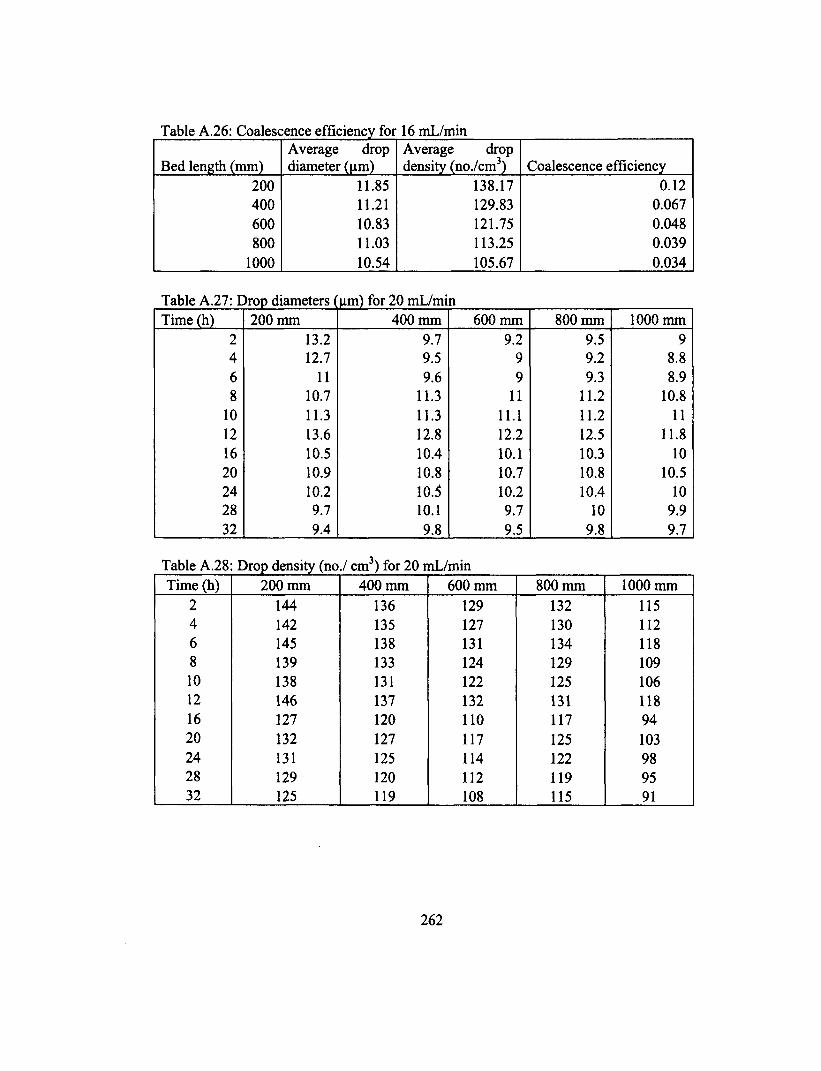
Table A.26: Coalescence efficiency for 16 mL/min
Bed length (mm) Average drop diameter (pm)
Average drop density (no./cm3) Coalescence efficiency
200 11.85 138.17 0.12 400 11.21 129.83 0.067 600 10.83 121.75 0.048 800 11.03 113.25 0.039
1000 10.54 105.67 0.034
Table A.27: Dron diameters(um) for 20 mL/min Time (h) 200 mm 400 mm 600 mm 800 mm 1000 mm
2 13.2 9.7 9.2 9.5 9 4 12.7 9.5 9 9.2 8.8 6 11 9.6 9 9.3 8.9 8 10.7 11.3 11 11.2 10.8
10 11.3 11.3 11.1 11.2 11 12 13.6 12.8 12.2 12.5 11.8 16 10.5 10.4 10.1 10.3 10 20 10.9 10.8 10.7 10.8 10.5 24 10.2 10.5 10.2 10.4 10 28 9.7 10.1 9.7 10 9.9 32 9.4 9.8 9.5 9.8 9.7
Table A.28 Drop density (no./ cm3) for 20 mL/min Time (h) 200 mm 400 mm 600 mm 800 mm 1000 mm
2 144 136 129 132 115 4 142 135 127 130 112 6 145 138 131 134 118 8 139 133 124 129 109 10 138 131 122 125 106 12 146 137 132 131 118 16 127 120 110 117 94 20 132 127 117 125 103 24 131 125 114 122 98 28 129 120 112 119 95 32 125 119 108 115 91
262
Table A.26: Coalescence efficiency for 16 mL/min
Bed length (mm) Average drop diameter (nm)
Average drop density (no./cm3) Coalescence efficiency
200 11.85 138.17 0.12
400 11.21 129.83 0.067
600 10.83 121.75 0.048
800 11.03 113.25 0.039
1000 10.54 105.67 0.034
Table A.27: Drop diameters ("nm) for 20 mL/min
Time (h) 200 mm 400 mm 600 mm 800 mm 1000 mm
2 13.2 9.7 9.2 9.5 9
4 12.7 9.5 9 9.2 8.8
6 11 9.6 9 9.3 8.9
8 10.7 11.3 11 11.2 10.8
10 11.3 11.3 11.1 11.2 11
12 13.6 12.8 12.2 12.5 11.8
16 10.5 10.4 10.1 10.3 10
20 10.9 10.8 10.7 10.8 10.5
24 10.2 10.5 10.2 10.4 10 28 9.7 10.1 9.7 10 9.9
32 9.4 9.8 9.5 9.8 9.7
Table A.28: Drop density (no./ cm3) for 20 mL/min
Time (h) 200 mm 400 mm 600 mm 800 mm 1000 mm
2 144 136 129 132 115
4 142 135 127 130 112 6 145 138 131 134 118 8 139 133 124 129 109 10 138 131 122 125 106 12 146 137 132 131 118 16 127 120 110 117 94 20 132 127 117 125 103
24 131 125 114 122 98 28 129 120 112 119 95 32 125 119 108 115 91
262

Table A.29: Coalescence efficiency for 20 mL/min
Bed length (mm) Average drop diameter (p.m)
Average drop density (no./cm3)
Coalescence efficiency
200 11.3 134.5 0.100 400 9.75 127.5 0.0536 600 9.35 118.5 0.0389 800 9.65 123.5 0.0279
1000 9.35 103.0 0.0270
Table A.30: Dron diameters In for 24 mL/min Time (h) 200 mm 400 mrn 600 nun 800 mm 1000 mm
2 13.9 13.4 12.8 13.1 12.3 4 13.2 12.9 12.4 12.7 12.1 6 10.4 12.6 12.1 12.4 11.8 8 11.3 10.7 10.1 10.4 9.7
10 10.9 10 9.4 9.7 9 12 14.4 13.5 12.9 13.2 12.6 16 11.2 10.9 10.3 10.7 9.8 20 12.1 11.2 10.5 10.9 10.2 24 10.9 9.8 9.2 9.5 8.9 28 11.3 10.8 10.1 10.5 9.6
Table A.31 Drop density (no / cm3) for 24 mL/min Time (h) 200 mm 400 mm 600 mm 800 mm 1000 mm
2 165 135 128 120 111 4 161 133 125 118 110 6 155 145 139 115 108 8 138 126 119 110 98 10 132 123 115 106 92 12 166 146 129 119 112 16 137 125 118 107 96 20 142 129 121 112 100 24 135 124 116 104 93 28 131 121 113 101 90
263
Table A.29: Coalescence efficiency for 20 mL/min
Bed length (mm) Average drop diameter (|im)
Average drop density (no./cm3)
Coalescence efficiency
200 11.3 134.5 0.100
400 9.75 127.5 0.0536
600 9.35 118.5 0.0389
800 9.65 123.5 0.0279
1000 9.35 103.0 0.0270
Table A.30: Drop diameters (urn) for 24 mL/min
Time (h) 200 mm 400 mm 600 mm 800 mm 1000 mm
2 13.9 13.4 12.8 13.1 12.3
4 13.2 12.9 12.4 12.7 12.1
6 10.4 12.6 12.1 12.4 11.8
8 11.3 10.7 10.1 10.4 9.7
10 10.9 10 9.4 9.7 9
12 14.4 13.5 12.9 13.2 12.6
16 11.2 10.9 10.3 10.7 9.8
20 12.1 11.2 10.5 10.9 10.2
24 10.9 9.8 9.2 9.5 8.9
28 11.3 10.8 10.1 10.5 9.6
Table A.31: Drop density (no./ cm3) for 24 mL/min
Time (h) 200 mm 400 mm 600 mm 800 mm 1000 mm
2 165 135 128 120 111
4 161 133 125 118 110 6 155 145 139 115 108 8 138 126 119 110 98 10 132 123 115 106 92 12 166 146 129 119 112 16 137 125 118 107 96 20 142 129 121 112 100 24 135 124 116 104 93 28 131 121 113 101 90
263

Table A.32: Coalescence efficiency for 24 mL/min
Bed length (mm) Average drop diameter (gm)
Average drop density (no./cm3)
Coalescence efficiency
200 12.6 148 0.081 400 12.1 128 0.053 600 11.45 120.5 0.039 800 11.8 110.5 0.032
1000 10.95 100.5 0.025
Table A.33: Drop diameters(um) for 28 mL/min Time (h) 200 mm 400 mm 600 mm 800 mm 1000 mm
2 14.7 13.4 12.7 13.1 12.4 4 13.6 12.2 11.5 11.8 11.2 6 12.4 11.7 11.1 11.4 10.7 8 11.1 10.8 10.2 10.5 9.8
10 14.3 13.1 12.5 12.9 12.1 12 10.8 10.1 9.5 9.7 9.1 16 11 10.5 9.9 10.2 9.3 20 10.3 9.8 9 9.3 8.5
Table A.34: Drop density (no.! cm3) for 28 rnL/min Time (h) 200 mm 400 mm 600 mm 800 mm 1000 mm
2 149 137 131 121 109 4 142 132 126 116 103 6 139 128 121 112 101 8 136 125 118 103 99 10 140 130 123 113 102 12 129 121 112 99 94 16 131 122 115 100 97 20 126 119 111 98 91
Table A.35: Coalescence efficiency for 28 mL/min
Bed length (mm) Average drop diameter (Am)
Average drop density (no./cm3)
Coalescence efficiency
200 12.5 137.5 0.080 400 11.6 128 0.047 600 10.85 121 0.035 800 11.2 109.5 0.029
1000 10.45 100 0.023
264
Table A.32: Coalescence efficiency for 24 mL/min
Bed length (mm) Average drop diameter (um)
Average drop density (no./cm3)
Coalescence efficiency
200 12.6 148 0.081
400 12.1 128 0.053
600 11.45 120.5 0.039
800 11.8 110.5 0.032
1000 10.95 100.5 0.025
Table A.33: Drop diameters (nm) for 28 mL/min
Time (h) 200 mm 400 mm 600 mm 800 mm 1000 mm
2 14.7 13.4 12.7 13.1 12.4
4 13.6 12.2 11.5 11.8 11.2
6 12.4 11.7 11.1 11.4 10.7
8 11.1 10.8 10.2 10.5 9.8
10 14.3 13.1 12.5 12.9 12.1
12 10.8 10.1 9.5 9.7 9.1
16 11 10.5 9.9 10.2 9.3
20 10.3 9.8 9 9.3 8.5
Table A.34: Drop density (no./ cm3) for 28 mL/min
Time (h) 200 mm 400 mm 600 mm 800 mm 1000 mm
2 149 137 131 121 109
4 142 132 126 116 103
6 139 128 121 112 101 8 136 125 118 103 99
10 140 130 123 113 102 12 129 121 112 99 94 16 131 122 115 100 97
20 126 119 111 98 91
Table A.35: Coalescence efficiency for 28 mL/min
Bed length (mm) Average drop diameter (um)
Average drop density (no./cm3)
Coalescence efficiency
200 12.5 137.5 0.080 400 11.6 128 0.047 600 10.85 121 0.035
800 11.2 109.5 0.029
1000 10.45 100 0.023
264

Table A.36: Dron diameters In for 32 mL/min Time (h) 200 mm 400 mm 600 mm 800 mm 1000 mm 2 14.1 13.3 12.5 12.8 12.1 4 13.7 12.6 11.8 12.3 11.6 6 11.7 11.2 10.7 10.9 10.3 8 12.6 12.1 11.5 11.9 11.2 10 11.9 11 10.2 10.5 10 12 10.5 9.8 9.1 9.5 8.7 16 11.1 10.5 9.6 10.1 9.2
Table A.37: Drop density no./ cm3) for 32 mL/min Time (h) 200 mm 400 mm 600 mm 800 mm 1000 mm
2 136 124 119 115 110 4 133 120 116 112 107 6 129 117 115 109 103 8 135 122 117 113 109 10 131 119 112 109 104 12 121 115 107 100 92 16 125 117 109 103 96
Table A.38: Coalescence efficiency for 32 mL/min
Bed length (mm) Average drop diameter (gm)
Average drop density (no./cm3)
Coalescence efficiency
200 12.60 130.5 0.081 400 11.90 120.5 0.047 600 11.05 114.0 0.033 800 11.45 109.0 0.026
1000 10.65 103.0 0.021
Table A.39: Data used to fit Crickmore model
Flow rate, rnL/min
Initial oil concentration (Co), mg/L
Effluent oil concentration (C), mg/L Time, h t', h/cm2 In (C/Co)
12 50 44.2 50 88.407 -0.123 16 50 45.4 38 69.845 -0.096 20 50 46.1 32 61.113 -0.0812 24 50 46.2 28 54.272 -0.0790 28 50 47.1 20 39.549 -0.0596 32 50 46.8 16 32.068 -0.066
265
Table A.36: Drop diameters (urn) for 32 mL/min Time (h) 200 mm 400 mm 600 mm 800 mm 1000 mm 2 14.1 13.3 12.5 12.8 12.1 4 13.7 12.6 11.8 12.3 11.6 6 11.7 11.2 10.7 10.9 10.3 8 12.6 12.1 11.5 11.9 11.2 10 11.9 11 10.2 10.5 10 12 10.5 9.8 9.1 9.5 8.7 16 11.1 10.5 9.6 10.1 9.2
Table A.37: Drop density (no./ cm3) for 32 mL/min Time (h) 200 mm 400 mm 600 mm 800 mm 1000 mm
2 136 124 119 115 110 4 133 120 116 112 107 6 129 117 115 109 103 8 135 122 117 113 109 10 131 119 112 109 104 12 121 115 107 100 92 16 125 117 109 103 96
Table A.38: Coalescence efficiency for 32 mL/min
Bed length (mm) Average drop diameter (|im)
Average drop density (no./cm3)
Coalescence efficiency
200 12.60 130.5 0.081 400 11.90 120.5 0.047 600 11.05 114.0 0.033 800 11.45 109.0 0.026
1000 10.65 103.0 0.021
Table A.39: Data used to fit Cric cmore model Initial oil Effluent oil
Flow rate, concentration concentration mL/min (Co), mg/L (C), mg/L Time, h t', h/cm2 In (C/Co)
12 50 44.2 50 88.407 -0.123 16 50 45.4 38 69.845 -0.096 20 50 46.1 32 61.113 -0.0812 24 50 46.2 28 54.272 -0.0790 28 50 47.1 20 39.549 -0.0596 32 50 46.8 16 32.068 -0.066
265
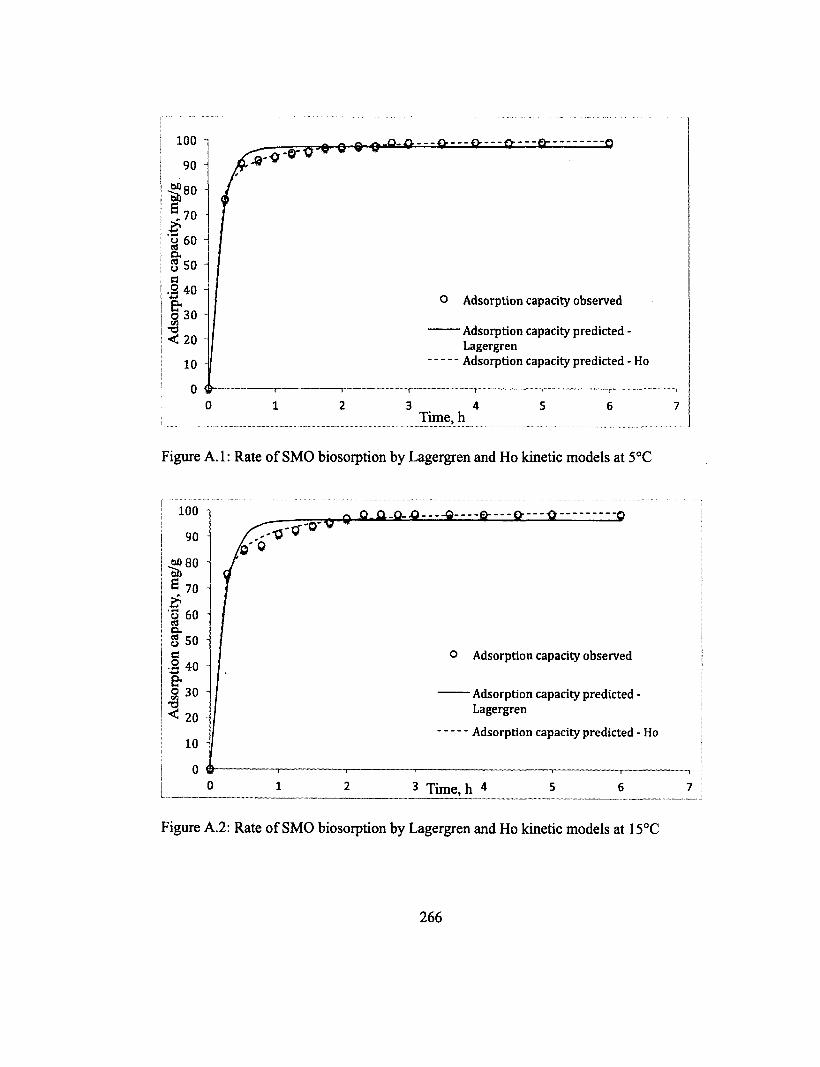
1 380
5, 70
60
8 so ..52 40
oo 30
d••t
20
10
0
0 Adsorption capacity observed
Adsorption capacity predicted -Lagergren Adsorption capacity predicted - Ho
3 4 Time, h
Figure A.1: Rate of SMO biosorption by Lagergren and Ho kinetic models at 5°C
100
90
ho 80
5 70
c.) 60 cs, 5 so
40
30 -66
20
10
0 0
"0" -0- - - - 4-
0 Adsorption capacity observed
Adsorption capacity predicted -Lagergren
Adsorption capacity predicted - Ho
3 Time, h 4
Figure A.2: Rate of SMO biosorption by Lagergren and Ho kinetic models at 15°C
266
100 - - - - o
.2 40 -o Adsorption capacity observed
o 30 -
3 < 20 -Adsorption capacity predicted -Lagergren Adsorption capacity predicted - Ho
Time, h
Figure A. 1: Rate of SMO biosorption by Lagergren and Ho kinetic models at 5°C
100 i
/q'Q
9-
O Adsorption capacity observed
Adsorption capacity predicted -Lagergren
Adsorption capacity predicted - Ho
0 1 2 3 Time, h 4 5 6 7
Figure A.2: Rate of SMO biosorption by Lagergren and Ho kinetic models at 15°C
266

Ads
orpt
ion
capa
city
, mg/
g
100
80
60
40
20
0
o Adsorption capacity observed
Adsorption capacity predicted - Lagergren
Adsorption capacity predicted - Ho
0 3 Time, h
Figure A.3: Rate of SMO biosorption by Lagergren and Ho kinetic models at 30°C
98.4
98.2 -
to 98.0 - --a) E 97.8 - -6 .5 97.6vs cd • 97.4
. 0 97.2
O 97.0 - •t1 < 96.8
96.6
Q -
o Adsorption capacity observed
Adsorption capacity predicted - Lagergren
Adsorption capacity predicted - Ho
3 4 Time, h
5
Figure A.4: Rate of CO biosorption by Lagergren and Ho kinetic models at 5°C
267
100
80
Ph 60
40
o Adsorption capacity observed
Adsorption capacity predicted - Lagergren
Adsorption capacity predicted - Ho
20
0 3 Time, h 4 0 2 1 5 6 7
Figure A.3: Rate of SMO biosorption by Lagergren and Ho kinetic models at 30°C
I5
& 8* o a o ••p & o •8 <
98.4
98.2
98.0
97.8
97.6
97.4
97.2
97.0
96.8
96.6
o 9 Q.o.ft-Q-fr-9'Q"" 0 o ® ? 0
o Adsorption capacity observed
Adsorption capacity predicted - Lagergren
Adsorption capacity predicted - Ho
3 Time, h 4
Figure A.4: Rate of CO biosorption by Lagergren and Ho kinetic models at 5°C
267

98.5
ao 98.0
5 X97.5
"c"3 co
6' 97.0
0
46 , 96.5 I
96.0
95.5 0
0 Adsorption capacity observed
Adsorption capacity predicted - Lagergren
Adsorption capacity predicted - Ho
3 Time, h 4
Figure A.5: Rate of CO biosorption by Lagergren and Ho kinetic models at 15°C
98.5
98.0
11137.5
,s5 97.0
896.5 • 1.1
95.5
o Adsorption capacity observed
Adsorption capacity predicted -Lagergren
Adsorption capacity predicted - Ho
3 Time, h 7
Figure A.6: Rate of CO biosorption by Lagergren and Ho kinetic models at 30°C
268
98.5
bo 98.0
I £97.5 G
S 97.0 a o
1*96.5 o •8 ^ 96.0
95.5
9 qq g 'o""Q
O Adsorption capacity observed
Adsorption capacity predicted - Lagergren
Adsorption capacity predicted - Ho
3 Time, h 4
Figure A.5: Rate of CO biosorption by Lagergren and Ho kinetic models at 15°C
98.5
98.0
f»7.5
897.0 & o §96.5
*•£3
&
J96.0 <
95.5
0 o 0 o..0-o-q-Q"Q""o""6""o" 0 ?
p o Adsorption capacity observed
• Adsorption capacity predicted -Lagergren
Adsorption capacity predicted - Ho
3 Time, h 4
Figure A.6: Rate of CO biosorption by Lagergren and Ho kinetic models at 30°C
268

98.5
bo 98.0
5 .6 97.5 Z)
COQ
97.0 0
4-6 o 96.5
96.0
95.5
o Adsorption capacity observed
Adsorption capacity predicted - Lagergren
Adsorption capacity predicted - Ho
0 1 2 3 Ti
4 Time, h
Figure A.7: Rate of Bright-Edge 80 biosorption by Lagergren and Ho models at 5°C
98.5
98.0
ao -a) 97.5 5
.6 97.0
ct ▪ 96.5 U
.9. • 96.0 - 46' - • 95.5
95.0
94.5
L
-- -------------------------
o Adsorption capacity observed
Adsorption capacity predicted - Lagergren
Adsorption capacity predicted - Ho
3 Time, h 4 5
Figure A.8: Rate of Bright-Edge 80 biosorption by Lagergren and Ho models at 15°C
269
98.5
to 98.0
I
£ 97-5
8 & u 97.0 C o v» fr o 96.5 •8 <
96.0
95.5
q Q g q"—2 9 Q. SL
o Adsorption capacity observed
• Adsorption capacity predicted - Lagergren
Adsorption capacity predicted - Ho
Time, h
Figure A.7: Rate of Bright-Edge 80 biosorption by Lagergren and Ho models at 5°C
98.5
98.0
bo ~Sb 97.5 £
& 97.0
U 03-96.5 Q
•2 96.0
&
J 95.5 <
95.0
94.5
o q oq.-q-o-q~o~q~ 0 q q_ 9
o Adsorption capacity observed
Adsorption capacity predicted - Lagergren
Adsorption capacity predicted - Ho
3 Time, h 4
Figure A.8: Rate of Bright-Edge 80 biosorption by Lagergren and Ho models at 15°C
269

Ads
orpt
ion
capa
city
, mg/
g
98.5 -
98.0 -
97.5
97.0
96.5 -
96.0
95.5
95.0 -
94.5
94.0
93.5
----------------------------------
0 Adsorption capacity observed
Adsorption capacity predicted -Lagergren
Adsorption capacity predicted - Ho
3 Time, h 4 7
Figure A.9: Rate of Bright-Edge 80 biosorption by Lagergren and Ho models at 30°C
Ads
orbt
ion
capa
city
, Q m
g/g
105
100
95
90
85
80
75
0 0
0 0
o Adsorption capacity -Observed
—Adsorption capacity - Predicted
o
05 0.7 0.9 1.3 1.5 1.7
Figure A.10: Rate of SMO biosorption by intra-particle diffusion model at 5°C
270
1.9
1 c3 & o d o
• m +->
& o •3 <
98.5
98.0
97.5
97.0
96.5
96.0
95.5
95.0
94.5
94.0
93.5
0 0 gL.Q 0-Q"P"o""0 * Q 0 2 0-
O Adsorption capacity observed
• Adsorption capacity predicted -Lagergren
Adsorption capacity predicted - Ho
3 Time, h 4
Figure A.9: Rate of Bright-Edge 80 biosorption by Lagergren and Ho models at 30°C
105 -i
o Adsorption capacity -Observed
Adsorption capacity - Predicted
Vt, h0-5
Figure A. 10: Rate of SMO biosorption by intra-particle diffusion model at 5°C
270

105
100
11)E 95 0'
.. ,..' 90 O RS cl. 8 85 = 0 2 80 0 ...
-6' ..:t 75
05 0.7 0.9
o Adsorption capacity -Observed
— Adsorption capacity - Predicted
1.1 'Nit, 110.5
1.3 1.5
Figure A.11: Rate of SMO biosorption by intra-particle diffusion model at 15°C
97
to - 92 E 0' p: 87 0 is to. RS O • 82 2
:r:i 4.4
., • 77 d
72
O
0 O
0 0
o Adsorption capacity -Observed
Adsorption capacity - Predicted
1.7
0 5 0.7 0.9 1.1
lit, 11°.5
1.3 1.5 1.7
Figure A.12: Rate of SMO biosorption by intra-particle diffusion model at 22°C
271
105
100 oo
S 95
8«
° Adsorption capacity -Observed
Adsorption capacity - Predicted j3 80 o M TJ < 75
0.5 0.7 0.9 1.1 1.5 1.7 1.3
Vt, h0-5
Figure A. 11: Rate of SMO biosorption by intra-particle diffiision model at 15°C
97
©«
82
-£ o -3 77
o Adsorption capacity -Observed
Adsorption capacity - Predicted
72 0.5 0.7 1.5 1.3 1.7
Vt, h0-5
Figure A. 12: Rate of SMO biosorption by intra-particle diffusion model at 22°C
271

103
98
0 E 93
CY
88 art
0 83
0 -1:1 78 44t 0.5 0.6 0.7 0.8 0.9 1 1.1 1.2 1.3
h"
0 • 0
0 Adsorption capacity -Observed
—Adsorption capacity - Predicted
Figure A.13: Rate of SMO biosorption by intra-particle diffusion model at 30°C
1 )1)E
.6
0
A
99
98.5
0
98
97.5 •
0 Adsorption capacity -Observed
97 —Adsorption capacity - Predicted
96.5 0 5 0.6 0.7 0.8 0.9 1 1.1 1.2 1.3
h"
Figure A.14: Rate of CO biosorption by intra-particle diffusion model at 5°C
272
103
6 93
u 88
O 83 o Adsorption capacity -Observed
Adsorption capacity - Predicted
1.2 0.6 0.7 0.8
Figure A. 13: Rate of SMO biosorption by intra-particle diffusion model at 30°C
"5b 98.5
o Adsorption capacity -Observed
Adsorption capacity - Predicted •3 97
Figure A. 14: Rate of CO biosorption by intra-particle diffusion model at 5°C
272

99
98.5
04 98
E 0 '97.5
97
uo 96.5 0
-° 96
< 95.5 05
0
o Adsorption capacity -Observed
— Adsorption capacity - Predicted
0
0.6 0.7 0.8 0.9 Alt, 110.5
1 1.1 1.2
Figure A.15: Rate of CO biosorption by intra-particle diffusion model at 15°C
99
98
to 97
E 96
F. 95
94
e) 93 0
,14 92
.g 91 90
05 0.7 0.9 1.1
0
o Adsorption capacity -Observed
Adsorption capacity - Predicted
h"
1.3 1.5
Figure A.16: Rate of CO biosorption by intra-particle diffusion model at 22°C
273
1.3
1.7
98.5
° Adsorption capacity -Observed 96.5
Adsorption capacity - Predicted
<95.5
1.2 1.3 0.5 0.6 0.7 0.8 0.9 1.1 1 Vt, h0 5
Figure A. 15: Rate of CO biosorption by intra-particle diffusion model at 15°C
° Adsorption capacity -Observed
—Adsorption capacity - Predicted
1.1
Vt, h0-5
Figure A. 16: Rate of CO biosorption by intra-particle diffusion model at 22°C
273

Ads
orbt
ion
capa
city
, Q m
g/g
99
98.5
98 0 0
97.5
97
96.5
96
95.5
95
94.5 0 5 0.55 0.6 0.65 0.7 0.75 0.8 0.85 0.9
119.5
o Adsorption capacity -Observed
— Adsorption capacity - Predicted
Figure A.17: Rate of CO biosorption by intra-particle diffusion model at 30°C
98.5
98
143E 97.5
0 1
-41.; 97
c) 96.5 0
6- 96
d 95.5
05
O
0
o Adsorption capacity -Observed
—Adsorption capacity - Predicted
0.6 0.7 0.8
'It, 11.0.5
0.9 1.1 1.2
Figure A.18: Rate of Bright-Edge 80 biosorption by intra-particle diffusion model at 5°C
274
99
98.5
97.5
97
g, 96.5
96
o Adsorption capacity -Observed
—Adsorption capacity - Predicted 95
94.5
0.8 0.85 0.9 0.55 0.75 0.5 0.65
Figure A. 17: Rate of CO biosorption by intra-particle diffusion model at 30°C
98.5
6 97.5
& ° 96.5
o Adsorption capacity -Observed
Adsorption capacity - Predicted
95.5
0.5 0.7 0.6 0.8 0.9
Vt, h0-5
Figure A. 18: Rate of Bright-Edge 80 biosorption by intra-particle diffusion model at 5°C
274

99
98.5
0 98 a) E 97.5 a i, 97
a 96.5cs cc.)
96 0
€ :a 95.5 0 434 95 <
94.5 05
0
0
o Adsorption capacity -Observed
—Adsorption capacity - Predicted
0.6 0.7 0.8 0.9
'It, V.51 1.1 1.2
Figure A.19: Rate of Bright-Edge 80 biosorption by intra-particle diffusion model at 15°C
Ads
orbt
ion
capa
city
, Q m
g/g
98.5
98
97.5
97
96.5
96
95.5
95
94.5
94
93.5 05 0.6 0.7
0 0
o Adsorption capacity -Observed — Adsorption capacity - Predicted
0.8 0.9
Alt, ha5
1 1.1 1.2 1.3
Figure A.20: Rate of Bright-Edge 80 biosorption by intra-particle diffusion model at 22°C
275
98.5
E 97.5
8 96.5
95.5 o Adsorption capacity -Observed
—Adsorption capacity - Predicted
94.5
1.2 1.1 0.7 0.8 0.9 1 0.5 0.6
Vt, h°-5
Figure A. 19: Rate of Bright-Edge 80 biosorption by intra-particle diffusion model at 15°C
98.5 i
o Adsorption capacity -Observed
—Adsorption capacity - Predicted
93.5 ~i > 1 1 1 1 1 1 1
0.5 0.6 0.7 0.8 0.9 1 1.1 1.2 1.3
Vt, h0-5
Figure A.20: Rate of Bright-Edge 80 biosorption by intra-particle diffusion model at 22°C
275

Ads
orbt
ion
capa
city
, Q m
g/g
98.4
98.2
98
97.8
97.6
97.4
97.2
97
96.8
96.6
96.4 05
0
0
o Adsorption capacity -Observed —Adsorption capacity - Predicted
0.6 0.7 0.8
h"
0.9 1 1.1
Figure A.21: Rate of Bright-Edge 80 biosorption by intra-particle diffusion model at 30°C
L
700
600 ao
E 500 e,os 400
g 300
en9, 200
•cs
100
0
0 Experimental
Langmuir predicted
Freundlich predicted
10 15 Ce, mg/L
20
Figure A.22: The Langmuir and Freundlich isotherm for biosorption of SMO at 5°C
276
25
98.4 i
o Adsorption capacity -Observed
—Adsorption capacity - Predicted
< )
96.4 4 . . 1 . . .
0.5 0.6 0.7 0.8 0.9 1 1.1
Vt, h05
Figure A.21: Rate of Bright-Edge 80 biosorption by intra-particle diffusion model at 30°C
700
600
500
« 400
300
O Experimental
Langmuir predicted
Freundlich predicted
g 200
100
0 0 5 10 15 20 25
Ce, mg/L
Figure A.22: The Langmuir and Freundlich isotherm for biosorption of SMO at 5°C
276

700
600 to be g 500
co 400
gi 300
200
100
0 0
o Experimental
Langmuir predicted
Freundlich predicted
10 15 Ce, mg/L
20 25
Figure A.23: The Langmuir and Freundlich isotherm for biosorption of SMO at 15°C
700
600 eo too
500
eo 400
300
200
100
0 10 15
Ce, mg/L
o Experimental
Langmuir predicted
Freundlich predicted
20 25 30
Figure A.24: The Langmuir and Freundlich isotherm for biosorption of SMO at 22°C
277
700
BO S 500
g 200
O Experimental
Langmuir predicted
Freundlich predicted
10 ^ /. 15 Ce, mg/L
20 25
Figure A.23: The Langmuir and Freundlich isotherm for biosorption of SMO at 15°C
700
600
M g 500
S 400
O Experimental
Langmuir predicted
Freundlich predicted
15 Ce, mg/L
20 25 30
Figure A.24: The Langmuir and Freundlich isotherm for biosorption of SMO at 22°C
277

700
ba 600
soo a 400 a g 300
I :0 P.
200
4< 100
0 0
o Experimental
Langmuir predicted
Freundlich predicted
10 15 20 25 Ce, mg/L
Figure A.25: The Langmuir and Freundlich isotherm for biosorption of CO at 5°C
600 OD
itik 500
.0 es 400
300
100
10 15 Ce, mg/L
Experimental
Langmuir predicted
Freundlich predicted
20
Figure A.26: The Langmuir and Freundlich isotherm for biosorption of CO at 22 °C
278
700
600
500
400
O Experimental
Langmuir predicted
Freundlich predicted
300
200
100
0 0 5 10 15 20 25
Ce, mg/L
Figure A.25: The Langmuir and Freundlich isotherm for biosorption of CO at 5°C
700
600
500
400
300 O Experimental
Langmuir predicted
Freundlich predicted
200
100
0 0 5 10 15 20 25 Ce, mg/L
Figure A.26: The Langmuir and Freundlich isotherm for biosorption of CO at 22 °C
278

700
600
iha 500
x. 400
I 8 g 300 0BA.
0 200
100 Q
0 5
--r
10
o Experimental
Langmuir predicted
Freundlich predicted
1
15 20 25 Ce, mg/L
Figure A.27: The Langmuir and Freundlich isotherm for biosorption of CO at 30°C
700
600 ba
r 500 jr ,400 a g 300
200
100
0
o Experimental
Langmuir predicted
Freundlich predicted
3
10 15 Ce, mg/L
20 25
Figure A.28: The Langmuir and Freundlich isotherm model plots for biosorption of Bright-Edge 80 at 5°C
279
700
„600 M S 500
S 400
£ 300 O Experimental
Langmuir predicted
Freundlich predicted
o 200
100
0 0 5 10 15 ,
Ce, mg/L 20 25 30
Figure A.27: The Langmuir and Freundlich isotherm for biosorption of CO at 30°C
700 1
600 as
if 500
300 -o Experimental
Langmuir predicted
Freundlich predicted
8 200 -
100
0 5 10 15 20 25 Ce, mg/L
Figure A.28: The Langmuir and Freundlich isotherm model plots for biosorption of Bright-Edge 80 at 5°C
279

700
ea 600 -1
g 500
1 . 400 -I 8 .1 300
• 200
[ ▪ 100 .1
0
o Experimental
Langmuir predicted
Freundlich predicted
10 15 20 25 30 35 40 1 Ce, mg/L
Figure A.29: The Langmuir and Freundlich isotherm model plots for biosorption of Bright-Edge 80 at 22°C
700
600 J [ IDA
soo
eta 400
O • 300
51 200
100
o Experimental
Langmuir predicted
Freundlich predicted
8 10 12 14 16 18 Ce, mg/L
Figure A.30: The Langmuir and Freundlich isotherm model plots for biosorption of Bright-Edge 80 at 30°C
280
700
600 H
S 500
2 400 -
O Experimental
Langmuir predicted
Freundlich predicted
300 -<
o 200
100
0 10 15 5 20 25 30 35 40 Ce, mg/L
Figure A.29: The Langmuir and Freundlich isotherm model plots for biosorption of Bright-Edge 80 at 22°C
700
600
« 400
o 300
Experimental
Langmuir predicted
Freundlich predicted
3 200
100
0 0 2 6 4 8 10 12 14 16 18
Ce, mg/L
Figure A.30: The Langmuir and Freundlich isotherm model plots for biosorption of Bright-Edge 80 at 30°C
280

1.0
0.9
0.8
0.7
0.6
$40.5
0.4
0.3
0.2
0.1
0.0
—Outman Predicted
• Experimental
0 500 1000 2000 2500 3000 Time
Figure A.31: Breakthrough curve predicted by Oulman model for SMO
1.0 1
0.9 -
0.8
0.7
0.6 -
0.5u
0.4
0.3
0.2 •
0.1 •
0.0
•
•
—Oulman Predicted
• Experimental
0 200 400 600 800 1000 1200 1400 1600 Time (min)
Figure A.32: Breakthrough curve predicted by Oulman model for CO
281
1.0
0.9
0.8
0.7
0.6 o ii.0.5 o
0.4
Oulman Predicted
• Experimental
0.3
0.2
0.1
2000 2500 0 500 1000 Timeim
3000 i
Figure A.31: Breakthrough curve predicted by Oulman model for SMO
l.o
0.9
0.8
0.7
0.6
Oulman Predicted
• Experimental 0.4
0.3
0.2
0.1
0.0 200 0 600 400 800 1000 1200 1400 1600
Time (min)
Figure A.32: Breakthrough curve predicted by Oulman model for CO
281

1.0
0.9
0.8
0.7
0.6 0Q0.5
0.4
0.3 J
0.2
0.1
0.0 0 200 400 600 800 1000 1200 1400 1600 1800 2000
Time (min)
— Oulman Predicted
• Experimental
Figure A.33: Breakthrough curve predicted by Oulman model for Bright-Edge 80
1.4
1.2
1 0.8
v
0.6
0.4
0.2
0
• Experimental
— Wolbroska Predicted
500 t(min)
Figure A.34: Breakthrough curve predicted by Wolbroska model for SMO
282
1000 I
1.0
0.9
0.8
0.7
0.6
Oulman Predicted 0.5
0.4 • Experimental
0.3
0.2
0.1
0.0 200 400 600 800 1000 1200 1400 1600 1800 2000 0
Time (mill)
Figure A.33: Breakthrough curve predicted by Oulman model for Bright-Edge 80
1.6
• Experimental
Wolbroska Predicted 1.4
1.2
ii 0.8
0.6
0.4
0.2
0 500 t(min)
1000
Figure A.34: Breakthrough curve predicted by Wolbroska model for SMO
282

• Experimental — Wolbroska Predicted
0 t.) (4 0.6
0 500 Time (min)
Figure A.35: Breakthrough curve predicted by Wolbroska model for CO
1.2
1
0.8
0.4
0.2
0 0
4
• Experimental — Wolbroska Predicted
4 4
TimiCOriin)
4
1000
Figure A.36: Breakthrough curve predicted by Wolbroska model for Bright-Edge 80
283
1.4
• Experimental
Wolbroska Predicted 1.2
1
0.8
0.6
0.4
0.2
0 0 500
Time (min) 1000
Figure A.35: Breakthrough curve predicted by Wolbroska model for CO
1.2
A Experimental
—Wolbroska Predicted 1
0.8
< 0.6
0.4
0.2
0 0 Timl^in) 1000
Figure A.36: Breakthrough curve predicted by Wolbroska model for Bright-Edge 80
283

Appendix B
Design of Batch and Column Adsorber System
Table B 1: Design of batch adsorber system for M rouxii biomass and SMO with a flow rate of 100 m3/d Descriptions Calculations Isotherm model used Freundlich Isotherm equation x/m = kCA(1/n) Isotherm constants
K 40.16 1/n (n = 1.12) 0.893
Initial oil concentration, mg/L 200 Final oil concentration, mg/L 5 Percentage of oil removal 97.5
=(40.16)(5)0.893)x/rn value mg/g
=168.99 =(100)(200-5)/1000
Mass of oil removed kg/d =19.5
Mass of biomass required using x/m value (kg/d) =(19.5)(1000)/(168.99) =115.39
Table B2: Design of batch adsorber system for M rouxii biomass and CO with a flow rate of 100 m3/d Descriptions Calculations Isotherm model used Freundlich Isotherm equation x/m = kCA(1/n) Isotherm constants
K 30.6 l/n (n = 1.01) 0.99
Initial oil concentration, mg/L 200 Final oil concentration, mg/L 5 Percentage of oil removal 97.5
x/m value mg/g =(30.6)(5)(0.99)=150.58
Mass of oil removed kg/d =(100)(200-5)/1000 =19.5
Mass of biomass required using x/m value (kg/d) =(19.5)(1000)/(150.58) =129.49
284
Appendix B
Design of Batch and Column Adsorber System
Table Bl: Design of batch adsorber system for M. rouxii biomass and SMO with a flow rate of 100 m3/d Descriptions Calculations Isotherm model used Isotherm equation Isotherm constants
K l/n(n = 1.12)
Initial oil concentration, mg/L Final oil concentration, mg/L Percentage of oil removal
x/m value mg/g
Mass of oil removed kg/d
Mass of biomass required using x/m value (kg/d)
Freundlich x/m = kCA(l/n)
40.16 0.893 200 5 97.5 =(40.16)(5)(0893)
=168.99 =(100)(200-5)/1000 =19.5 =(19.5)(1000)/(168.99) =115.39
Table B2: Design of batch adsorber system for M. rouxii biomass and CO with a flow rate of 100 m3/d Descriptions Calculations Isotherm model used Isotherm equation Isotherm constants
K l/n(n= 1.01)
Initial oil concentration, mg/L Final oil concentration, mg/L Percentage of oil removal
x/m value mg/g
Mass of oil removed kg/d
Mass of biomass required using x/m value (kg/d)
Freundlich x/m = kCA(l/n)
30.6 0.99 200 5 97.5 =(3O.6)(5)(0 99)
=150.58 =(100)(200-5)/1000 =19.5 =(19.5)(1000)/( 150.58) =129.49
284

Table B3: Design of batch adsorber system for M rouxii biomass and Bright-Edge 80 with a flow rate of 100 m3/d Descriptions Calculations Isotherm model used Freundlich Isotherm equation x/m = kCA(1/n) Isotherm constants
K 26.56 1/n (n = 1.16) 0.862
Initial oil concentration, mg/L 200 Final oil concentration, mg/L 5 Percentage of oil removal 97.5
x/m value mg/g =(26.56)(5)(0.862)
=106.36
Mass of oil removed kg/d =(100)(200-5)/1000 =19.5
Mass of biomass required using x/m value (kg/d) =(19.5)(1000)/(106.36) =183.33
285
Table B3: Design of batch adsorber system for M. rouxii biomass and Bright-Edge 80 with a flow rate of 100 m3/d Descriptions Calculations Isotherm model used Freundlich Isotherm equation x/m = kCA(l/n) Isotherm constants
K 26.56 l/n(n= 1.16) 0.862
Initial oil concentration, mg/L 200 Final oil concentration, mg/L 5 Percentage of oil removal
x/m value mg/g
97.5 =(26.56)(5)(0'862)
=106.36
Mass of oil removed kg/d =( 100)(200-5)/1000 =19.5
Mass of biomass required using x/m value (kg/d) =(19.5)(1000)/(106.36) =183.33
285

Table B4: Design of immobilized M rouxii biomass column filter for SMO with a flow rate of 100 m3/d By scale-up approach Flow rate, mL/min Unit liquid flow rate, L/h
Bed volume, cm3
Bed volume, L
Bed volume per unit time, BV/h
Design bed volume, m3
Inside diameter of column, mm Length of bed, mm Mass of biomass in the column, kg Packed density of biomass in the column, kg/m3Mass of immobilized biomass required, kg From breakthrough curve for allowable 10 mg/L oil concentration, the corresponding volume, L
Emulsion treated per kg of biomass, L/kg
Biomass exhausted per hour, kg/h
Breakthrough time, h
Breakthrough time, d
Breakthrough volume, m3
By kinetic approach
=2.6 =(2.6)(60)/1000 =0.156 =(3.14)(1.27)2(100)/4 =126.61 =126.61/1000 =0.127 =0.156/0.127 =1.23 =100/(1.23)(24) =3.38 =12.70 =300.00 =0.004500 =118.50 =400.74
=0.45
=0.45/0.0045 =100 =(100)(1000)/(100)(24) =41.67 =(400.74)/(41.67) =9.62 =9.62/24 =0.40074 =(0.40074)(100) =40.074
KT, L/h-kg (From Table 4.21) =4200 go, kg/kg (From Table 4.21) =0.0098 Co, mg/L =50 C, mg/L =5 Flow, m3/d =100 Flow, Q, L3/h =(100)(1000)/24 =4166.67
Volume, V, L3 =(40.074)(1000) =40074
Applying Thomas model solving for M, kg/h
(Equation 2.12) and 422.37
286
Table B4: Design of immobilized M. rouxii biomass column filter for SMO with a flow rate of 100 m3/d By scale-up approach Flow rate, mL/min =2.6
Unit liquid flow rate, L/h =(2.6)(60)/1000 =0.156
Bed volume, cm3 =(3.14)( 1.27)2( 100)/4 Bed volume, cm3
=126.61
Bed volume, L =126.61/1000 =0.127
Bed volume per unit time, BV/h =0.156/0.127 =1.23
Design bed volume, m3 =100/(1.23)(24) =3.38
Inside diameter of column, mm =12.70 Length of bed, mm =300.00 Mass of biomass in the column, kg =0.004500 Packed density of biomass in the column, kg/m3 =118.50 Mass of immobilized biomass required, kg =400.74 From breakthrough curve for allowable 10 mg/L oil =0.45 concentration, the corresponding volume, L
=0.45
Emulsion treated per kg of biomass, L/kg =0.45/0.0045 =100
Biomass exhausted per hour, kg/h =( 100)( 1000)/(100)(24) =41.67
Breakthrough time, h =(400.74)/(41.67) =9.62
Breakthrough time, d =9.62/24 =0.40074
Breakthrough volume, m3 =(0.40074)(100) =40.074
By kinetic approach Kt, L/h-kg (From Table 4.21) =4200 q0, kg/kg (From Table 4.21) =0.0098 Co, mg/L =50 C, mg/L =5
Flow, m3/d =100 Flow, Q, L3/h =(100)(1000)/24 =4166.67
Volume, V, L3 =(40.074)(1000) Volume, V, L3
-40074 Applying Thomas model (Equation 2.12) and 422.37 solving for M, kg/h
286

Table B5: Design of immobilized M rouxii biomass column filter for CO with a flow rate of 100 m3/d By scale-up approach Flow rate, mL/min Unit liquid flow rate, L/h
Bed volume, cm3
Bed volume, L
Bed volume per unit time, BV/h
Design bed volume, m3
Inside diameter of column, mm Length of bed, mm Mass of biomass in the column, kg Packed density of biomass in the column, kg/m3Mass of immobilized biomass required, kg From breakthrough curve for allowable 10 mg/L oil concentration, the corresponding volume, L
Emulsion treated per kg of biomass, L/kg
Biomass exhausted per hour, kg/h
Breakthrough time, h
Breakthrough time, d
Breakthrough volume, m3
By kinetic approach
=2.6 =(2.6)(60)/1000 =0.156 =(3.14)(1.27)2(100)/4 =126.61 =126.61/1000 =0.127 =0.156/0.127 =1.23 =100/(1.23)(24) =3.38 =12.70 =300.00 =0.0045 =118.50 =400.74
=0.08
=0.08/0.0045 =17.33 =(100)(1000)/(17.33)(24) =240.38 =(400.74)/(240.38) =1.67 =1.67/24 =0.069 =(0.069)(100) =6.95
KT, L/h-kg (From Table 4.21) =4980 qo, kg/kg (From Table 4.21) =0.0146 Co, mg/L =50 C, mg/L =5 Flow, m3/d =100 Flow, Q, L3/h =(100)(1000)/24 =4166.67
Volume, V, L3 =(6.95)(1000) =6950
Applying Thomas model (Equation solving for M, kg/h
2.12) and 149.72
287
Table B5: Design of immobilized M. rouxii biomass column filter for CO with a flow rate of 100 m3/d By scale-up approach Flow rate, mL/min =2.6
Unit liquid flow rate, L/h =(2.6)(60)/1000 =0.156
Bed volume, cm3 =(3.14)(1.27)2(100)/4 Bed volume, cm3
=126.61
Bed volume, L =126.61/1000 =0.127
Bed volume per unit time, BV/h =0.156/0.127 =1.23
Design bed volume, m3 =100/(1.23)(24) =3.38
Inside diameter of column, mm =12.70 Length of bed, mm =300.00 Mass of biomass in the column, kg =0.0045 Packed density of biomass in the column, kg/m3 =118.50 Mass of immobilized biomass required, kg =400.74 From breakthrough curve for allowable 10 mg/L oil =0.08
=0 08/0 0045 concentration, the corresponding volume, L
=0.08
=0 08/0 0045 Emulsion treated per kg of biomass, L/kg V*V W' V/• V/\y TmJ
=17.33
Biomass exhausted per hour, kg/h =(100)(1000)/(17.33)(24) =240.38
Breakthrough time, h =(400.74)/(240.38) =1.67
Breakthrough time, d =1.67/24 =0.069
Breakthrough volume, m3 =(0.069)(100) =6.95
By kinetic approach KT, L/h-kg (From Table 4.21) =4980 qo, kg/kg (From Table 4.21) =0.0146 Co, mg/L =50 C, mg/L =5
Flow, m3/d =100 Flow, Q, L3/h =(100)(1000)/24 =4166.67
Volume, V, L3 =(6.95)(1000) Volume, V, L3 =6950
Applying Thomas model (Equation 2.12) and 149.72 solving for M, kg/h
287

Table B6: Design of immobilized M rouxii biomass column filter for Bright-Edge 80 with a flow rate of 100 m3/d By scale-up approach Flow rate, mL/min Unit liquid flow rate, L/h
Bed volume, cm3
Bed volume, L
Bed volume per unit time, BV/h
Design bed volume, m3
Inside diameter of column, mm Length of bed, mm Mass of biomass in the column, kg Packed density of biomass in the column, kg/m3Mass of immobilized biomass required, kg From breakthrough curve for allowable 10 mg/L oil concentration, the corresponding volume, L
Emulsion treated per kg of biomass, L/kg
Biomass exhausted per hour, kg/h
Breakthrough time, h
Breakthrough time, d
Breakthrough volume, m3
By kinetic approach
=2.6 =(2.6)(60)/1000 =0.156 =(3.14)(1.27)2(100)14 =126.61 =126.61/1000 =0.127 =0.156/0.127 =1.23 =100/(1.23)(24) =3.38 =12.70 =300.00 =0.0045 =118.50 =400.74
=0.05
=0.05/0.0045 =11.11 =(100)(1000)/(11.11)(24) =375.0 =(400.74)/(375.0) =1.01 =1.01/24 =0.045 =(0.045)(100) =4.45
KT, L/h-kg (From Table 4.21) =3600 go, kg/kg (From Table 4.21) =0.0106 Co, mg/L =50 C, mg/L =5 Flow, m3/d =100 Flow, Q, L3/h =(100)(1000)/24 =4166.67
Volume, V, L3 =(4.45)(1000) =4450
Applying Thomas model (Equation solving for M, kg/h
2.12) and 260.904
288
Table B6: Design of immobilized M. rouxii biomass column filter for Bright-Edge 80 with a flow rate of 100 m3/d By scale-up approach Flow rate, mL/min =2.6
Unit liquid flow rate, L/h =(2.6)(60)/1000 =0.156
Bed volume, cm3 =(3.14)(1.27)2(100)/4 Bed volume, cm3
=126.61
Bed volume, L =126.61/1000
Bed volume, L =0.127
Bed volume per unit time, BV/h =0.156/0.127 =1.23
Design bed volume, m3 =100/(1.23)(24) =3.38
Inside diameter of column, mm =12.70 Length of bed, mm =300.00 Mass of biomass in the column, kg =0.0045 Packed density of biomass in the column, kg/m3 =118.50 Mass of immobilized biomass required, kg =400.74 From breakthrough curve for allowable 10 mg/L oil =0.05
=0 05/0 0045 concentration, the corresponding volume, L
=0.05
=0 05/0 0045 Emulsion treated per kg of biomass, L/kg ViVk/r \/< W i
= 11.11
Biomass exhausted per hour, kg/h =(100)(1000)/(11.11 )(24) =375.0
Breakthrough time, h =(400.74)/(375.0) =1.01
Breakthrough time, d =1.01/24 =0.045
Breakthrough volume, m3 =(0.045)(100) =4.45
By kinetic approach KT, L/h-kg (From Table 4.21) =3600 qo, kg/kg (From Table 4.21) =0.0106 Co, mg/L =50 C, mg/L =5
Flow, m3/d =100 Flow, Q, L3/h =(100)(1000)/24 =4166.67
Volume, V, L3 =(4.45)(1000) Volume, V, L3 =4450
Applying Thomas model (Equation 2.12) and 260.904 solving for M, kg/h
288