Embed Size (px)
Citation preview

Remote Sens. 2013, 5, 716-807; doi:10.3390/rs5020716OPEN ACCESS
Remote SensingISSN 2072-4292
www.mdpi.com/journal/remotesensing
Review
Recent Trend and Advance of Synthetic Aperture Radar withSelected TopicsKazuo Ouchi
Department of Computer Science, School of Electrical and Computer Engineering,National Defense Academy, 1-10-20 Hashirimizu, Yokosuka, Kanagawa 239-8686, Japan;E-Mail: [email protected]; Tel.: +81-46-841-3810 (ext. 3768); Fax: +81-46-844-5911
Received: 1 December 2012; in revised form: 14 January 2013 / Accepted: 16 January 2013 /Published: 5 February 2013
Abstract: The present article is an introductory paper in this special issue on syntheticaperture radar (SAR). A short review is presented on the recent trend and developmentof SAR and related techniques with selected topics, including the fields of applications,specifications of airborne and spaceborne SARs, and information contents in andinterpretations of amplitude data, interferometric SAR (InSAR) data, and polarimetric SAR(PolSAR) data. The review is by no means extensive, and as such only brief summaries ofof each selected topics and key references are provided. For further details, the readers arerecommended to read the literature given in the references theirin.
Keywords: synthetic aperture radar (SAR); recent development; amplitude information;interferometric SAR (InSAR); polarimetric SAR (PolSAR)
1. Introduction
In the 1985 Pioneer Award story [1], Carl Wiley, the inventor of SAR, stated with his modest manner:
I had the luck to conceive of the basic idea, which I called Doppler Beam Sharpening (DBS), ratherthan Synthetic Aperture Radar (SAR). Like all signal processing, there is a dual theory. One is afrequency-domain explanation. This is Doppler Beam Sharpening. If one prefers, one can analyzethe system in the time domain instead. This is SAR.
The conception of SAR was recorded in a Goodyear Aircraft report in 1951 by Wiley (note that theorigin of the aperture synthesis technique was an early phased array antenna called “bedspring antenna”
Remote Sens. 2013, 5 717
developed by Sir Watson-Watt in 1938 [2]), followed by the first SAR operation in 1952. Experimentscontinued with airborne SARs, and it was in 1978 when the first spaceborne SAR for earth observation onboard the SEASAT satellite was put into orbit. Despite its short lifetime of 106 days, SEASAT-SAR [3]was the pioneering mission which has lead the SAR technology to the present and future state-of-the-artstatus [4].
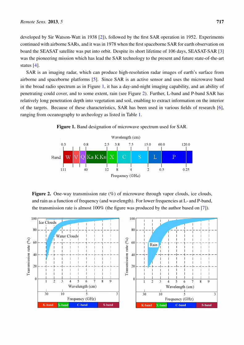
SAR is an imaging radar, which can produce high-resolution radar images of earth’s surface fromairborne and spaceborne platforms [5]. Since SAR is an active sensor and uses the microwave bandin the broad radio spectrum as in Figure 1, it has a day-and-night imaging capability, and an ability ofpenetrating could cover, and to some extent, rain (see Figure 2). Further, L-band and P-band SAR hasrelatively long penetration depth into vegetation and soil, enabling to extract information on the interiorof the targets. Because of these characteristics, SAR has been used in various fields of research [6],ranging from oceanography to archeology as listed in Table 1.
Figure 1. Band designation of microwave spectrum used for SAR.
Figure 2. One-way transmission rate (%) of microwave through vapor clouds, ice clouds,and rain as a function of frequency (and wavelength). For lower frequencies at L- and P-band,the transmission rate is almost 100% (the figure was produced by the author based on [7]).
Remote Sens. 2013, 5 718
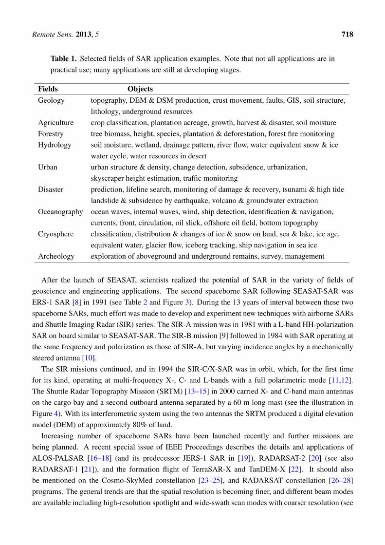
Table 1. Selected fields of SAR application examples. Note that not all applications are inpractical use; many applications are still at developing stages.
Fields ObjectsGeology topography, DEM & DSM production, crust movement, faults, GIS, soil structure,
lithology, underground resourcesAgriculture crop classification, plantation acreage, growth, harvest & disaster, soil moistureForestry tree biomass, height, species, plantation & deforestation, forest fire monitoringHydrology soil moisture, wetland, drainage pattern, river flow, water equivalent snow & ice
water cycle, water resources in desertUrban urban structure & density, change detection, subsidence, urbanization,
skyscraper height estimation, traffic monitoringDisaster prediction, lifeline search, monitoring of damage & recovery, tsunami & high tide
landslide & subsidence by earthquake, volcano & groundwater extractionOceanography ocean waves, internal waves, wind, ship detection, identification & navigation,
currents, front, circulation, oil slick, offshore oil field, bottom topographyCryosphere classification, distribution & changes of ice & snow on land, sea & lake, ice age,
equivalent water, glacier flow, iceberg tracking, ship navigation in sea iceArcheology exploration of aboveground and underground remains, survey, management
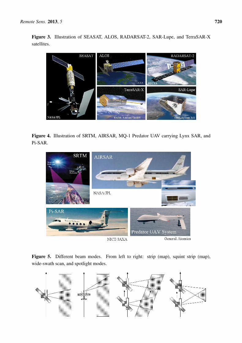
After the launch of SEASAT, scientists realized the potential of SAR in the variety of fields ofgeoscience and engineering applications. The second spaceborne SAR following SEASAT-SAR wasERS-1 SAR [8] in 1991 (see Table 2 and Figure 3). During the 13 years of interval between these twospaceborne SARs, much effort was made to develop and experiment new techniques with airborne SARsand Shuttle Imaging Radar (SIR) series. The SIR-A mission was in 1981 with a L-band HH-polarizationSAR on board similar to SEASAT-SAR. The SIR-B mission [9] followed in 1984 with SAR operating atthe same frequency and polarization as those of SIR-A, but varying incidence angles by a mechanicallysteered antenna [10].
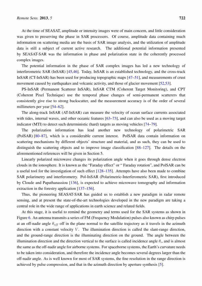
The SIR missions continued, and in 1994 the SIR-C/X-SAR was in orbit, which, for the first timefor its kind, operating at multi-frequency X-, C- and L-bands with a full polarimetric mode [11,12].The Shuttle Radar Topography Mission (SRTM) [13–15] in 2000 carried X- and C-band main antennason the cargo bay and a second outboard antenna separated by a 60 m long mast (see the illustration inFigure 4). With its interferometric system using the two antennas the SRTM produced a digital elevationmodel (DEM) of approximately 80% of land.
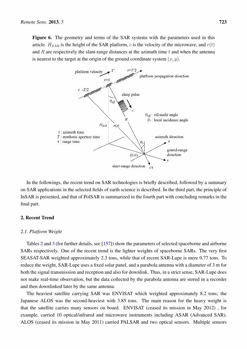
Increasing number of spaceborne SARs have been launched recently and further missions arebeing planned. A recent special issue of IEEE Proceedings describes the details and applications ofALOS-PALSAR [16–18] (and its predecessor JERS-1 SAR in [19]), RADARSAT-2 [20] (see alsoRADARSAT-1 [21]), and the formation flight of TerraSAR-X and TanDEM-X [22]. It should alsobe mentioned on the Cosmo-SkyMed constellation [23–25], and RADARSAT constellation [26–28]programs. The general trends are that the spatial resolution is becoming finer, and different beam modesare available including high-resolution spotlight and wide-swath scan modes with coarser resolution (see
Remote Sens. 2013, 5 719
Figure 5 for different bean modes). The conventional single-polarization mode is becoming dual or fullpolarimetric modes.
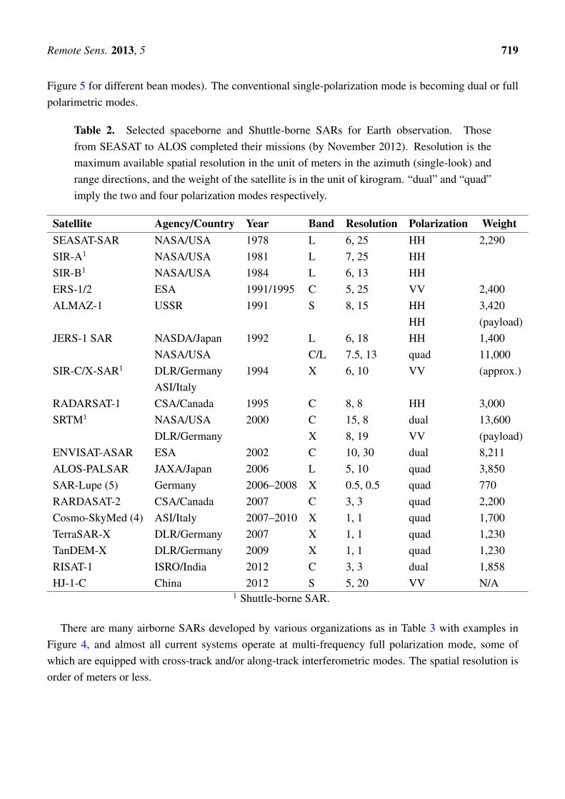
Table 2. Selected spaceborne and Shuttle-borne SARs for Earth observation. Thosefrom SEASAT to ALOS completed their missions (by November 2012). Resolution is themaximum available spatial resolution in the unit of meters in the azimuth (single-look) andrange directions, and the weight of the satellite is in the unit of kirogram. “dual” and “quad”imply the two and four polarization modes respectively.
Satellite Agency/Country Year Band Resolution Polarization WeightSEASAT-SAR NASA/USA 1978 L 6, 25 HH 2,290SIR-A1 NASA/USA 1981 L 7, 25 HHSIR-B1 NASA/USA 1984 L 6, 13 HHERS-1/2 ESA 1991/1995 C 5, 25 VV 2,400ALMAZ-1 USSR 1991 S 8, 15 HH 3,420
HH (payload)JERS-1 SAR NASDA/Japan 1992 L 6, 18 HH 1,400
NASA/USA C/L 7.5, 13 quad 11,000SIR-C/X-SAR1 DLR/Germany 1994 X 6, 10 VV (approx.)
ASI/ItalyRADARSAT-1 CSA/Canada 1995 C 8, 8 HH 3,000SRTM1 NASA/USA 2000 C 15, 8 dual 13,600
DLR/Germany X 8, 19 VV (payload)ENVISAT-ASAR ESA 2002 C 10, 30 dual 8,211ALOS-PALSAR JAXA/Japan 2006 L 5, 10 quad 3,850SAR-Lupe (5) Germany 2006–2008 X 0.5, 0.5 quad 770RARDASAT-2 CSA/Canada 2007 C 3, 3 quad 2,200Cosmo-SkyMed (4) ASI/Italy 2007–2010 X 1, 1 quad 1,700TerraSAR-X DLR/Germany 2007 X 1, 1 quad 1,230TanDEM-X DLR/Germany 2009 X 1, 1 quad 1,230RISAT-1 ISRO/India 2012 C 3, 3 dual 1,858HJ-1-C China 2012 S 5, 20 VV N/A
1 Shuttle-borne SAR.
There are many airborne SARs developed by various organizations as in Table 3 with examples inFigure 4, and almost all current systems operate at multi-frequency full polarization mode, some ofwhich are equipped with cross-track and/or along-track interferometric modes. The spatial resolution isorder of meters or less.
Remote Sens. 2013, 5 720
Figure 3. Illustration of SEASAT, ALOS, RADARSAT-2, SAR-Lupe, and TerraSAR-Xsatellites.
Figure 4. Illustration of SRTM, AIRSAR, MQ-1 Predator UAV carrying Lynx SAR, andPi-SAR.
Figure 5. Different beam modes. From left to right: strip (map), squint strip (map),wide-swath scan, and spotlight modes.

Remote Sens. 2013, 5 721
Table 3. Selected airborne SARs. Resolution is the maximum achievable spatial resolution(in general, at highest frequency band) in the unit of meters in the azimuth (single-look) andrange directions. Most of the listed airborne SARs can operate in the quad-polarization andinterferometric modes, except CALABAS and DBSAR. Lynx is an Unmanned/UninhabitedArial Vehicle (UAV)-borne SAR.
Sensor Agency/Counry Band ResolutionC/X-SAR CCRS/Canada X/C 0.9, 6AIRSAR NASA/USA C/X/L 0.6, 3E-SAR DLR/Germany X/C/S/L/P 0.3, 1F-SAR DLR/Germany X/C/S/L/P 0.3, 0.2Pi-SAR NICT, JAXA/Japan X/L 0.37, 3EMISAR DCRS/Denmark C/L 2, 2PHARUS TNO-FEL/Netherland C 1, 3Ingara DSTO/Australia X 0.15, 0.3RAMSES ONERA/France W/Ka/Ku/X/C/S/L/P 0.12, 0.12CALABAS FOA/Sewden HF/VHF 3, 3DBSAR NASA/USA L 10, 10UAVSAR NASA/USA L 1.0, 1.8Lynx Sandia/USA Ku 0.1, 0.1
Apart from spatial resolution and altitude, the main difference of airborne SARs is the requirement ofmotion compensation. The platform of spaceborne SARs is relatively stable, but the airborne SARs oftensuffer from platform instability caused by varying speed and/or motion of aircrafts. Since the azimuthreference signal assumes a stable platform path, the azimuth reference signal does not “match” the signalin raw data, and the images are degraded. It is, therefore, necessary to estimate the platform movementto produce a correct azimuth reference signal in order to form images of high quality by airborne SARs.There exist several motion compensation (also called autofocus) algorithms based on, for example,the onboard measurements, optimizing the image intensity of point-like targets, and the difference ininter-look image position in multi-look images e.g., [29,30]. These early post-processing algorithms(apart from the direct estimation by onboard sensors) include the multi-look registration or multi-lookmap drift algorithms [31,32], multi-look contrast optimization [33], prominent point processing [34],phase difference algorithm [35], and phase gradient algorithm [36,37]. These algorithms often sufferfrom long processing times. To shorten the processing time and/or to be applicable to scenes withoutprominent point-like targets, several algorithms have been proposed, including the phase adjustmentby contrast enhancement [38,39], autofocus by minimum-entropy [40], coherent map drift [41,42],and others [43,44]. It should be mentioned that spaceborne SARs, in particular interferometric SARs,sometimes suffer from image degradation by tropospheric and ionospheric effects as will be describedin Section 4.1.3. High-frequency airborne SARs may have some effects when imaging through denserain cells (see Figure 2 for microwave transmission rate), but in general, they are not affected by theatmospheric effects.
Remote Sens. 2013, 5 722
At the time of SEASAT, amplitude or intensity images were of main concern, and little considerationwas given to preserving the phase in SAR processors. Of course, amplitude data containing muchinformation on scattering media are the basis of SAR image analysis, and the utilization of amplitudedata is still a subject of current active research. The additional potential information presentedby SEASAT-SAR was the information in phase and polarization state in the coherently processedcomplex images.
The potential information in the phase of SAR complex images has led a new technology ofinterferometric SAR (InSAR) [45,46]. Today, InSAR is an established technology, and the cross-trackInSAR (CT-InSAR) has been used for producing topographic maps [47–51], and measurements of crustmovement caused by earthquakes and volcanic activity, and those of glacier movement [52,53].
PS-InSAR (Permanent Scatterer InSAR), InSAR CTM (Coherent Target Monitoring), and CPT(Coherent Pixel Technique) use the temporal phase changes of semi-permanent scatterers thatconsistently give rise to strong backscatter, and the measurement accuracy is of the order of severalmillimeters per year [54–62].
The along-track InSAR (AT-InSAR) can measure the velocity of ocean surface currents associatedwith tides, internal waves, and other oceanic features [63–73], and can also be used as a moving targetindicator (MTI) to detect such deterministic (hard) targets as moving vehicles [74–79].
The polarization information has lead another new technology of polarimetric SAR(PolSAR) [80–87], which is a considerable current interest. PolSAR data contain information onscattering mechanisms by different objects’ structure and material, and as such, they can be used todistinguish the scattering objects and to improve image classification [88–127]. The details on theaforementioned references will be given in Section 5.
Linearly polarized microwave changes its polarization angle when it goes through dense electronclouds in the ionosphere. It is known as the “Faraday effect” or “ Faraday rotation”, and PolSAR can bea useful tool for the investigation of such effect [128–135]. Attempts have also been made to combineSAR polarimetry and interferometry. Pol-InSAR (Polarimetric-Interferometric SAR), first introducedby Cloude and Papathanassiou [136], is expected to achieve microwave tomography and informationextraction in the forestry application [137–156].
Thus, the pioneering SEASAT-SAR has guided us to establish a new paradigm in radar remotesensing, and at present the state-of-the-art technologies developed in the new paradigm are taking acentral role in the wide range of applications in earth science and related fields.
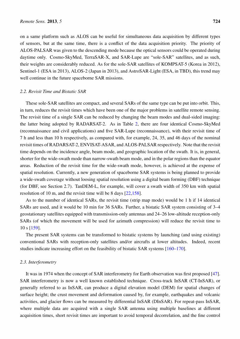
At this stage, it is useful to remind the geometry and terms used for the SAR systems as shown inFigure 6. An antenna transmits a series of FM (Frequency Modulation) pulses also known as chirp pulsesat an off-nadir angle θoff off in the plane normal to the satellite trajectory as it travels in the azimuthdirection with a constant velocity V . The illumination direction is called the slant-range direction,and the ground-range direction is the illuminating direction on the ground. The angle between theillumination direction and the direction vertical to the surface is called incidence angle θi, and is almostthe same as the off-nadir angle for airborne systems. For spaceborne systems, the Earth’s curvature needsto be taken into consideration, and therefore the incidence angle becomes several degrees larger than theoff-nadir angle. As is well known for most of SAR systems, the fine resolution in the range direction isachieved by pulse compression, and that in the azimuth direction by aperture synthesis [5].
Remote Sens. 2013, 5 723
Figure 6. The geometry and terms of the SAR systems with the parameters used in thisarticle. HSAR is the height of the SAR platform, c is the velocity of the microwave, and r(t)and R are respectively the slant-range distances at the azimuth time t and when the antennais nearest to the target at the origin of the ground coordinate system (x, y).
In the followings, the recent trend on SAR technologies is briefly described, followed by a summaryon SAR applications in the selected fields of earth science is described. In the third part, the principle ofInSAR is presented, and that of PolSAR is summarized in the fourth part with concluding remarks in thefinal part.
2. Recent Trend
2.1. Platform Weight
Tables 2 and 3 (for further details, see [157]) show the parameters of selected spaceborne and airborneSARs respectively. One of the recent trend is the lighter weights of spaceborne SARs. The very firstSEASAT-SAR weighted approximately 2.3 tons, while that of recent SAR-Lupe is mere 0.77 tons. Toreduce the weight, SAR-Lupe uses a fixed solar panel, and a parabola antenna with a diameter of 3 m forboth the signal transmission and reception and also for downlink. Thus, in a strict sense, SAR-Lupe doesnot make real-time observation, but the data collected by the parabola antenna are stored in a recorderand then downlinked later by the same antenna.
The heaviest satellite carrying SAR was ENVISAT which weighted approximately 8.2 tons; theJapanese ALOS was the second-heaviest with 3.85 tons. The main reason for the heavy weight isthat the satellite carries many sensors on board. ENVISAT (ceased its mission in May 2012) , forexample, carried 10 optical/infrared and microwave instruments including ASAR (Advanced SAR).ALOS (ceased its mission in May 2011) carried PALSAR and two optical sensors. Multiple sensors
Remote Sens. 2013, 5 724
on a same platform such as ALOS can be useful for simultaneous data acquisition by different typesof sensors, but at the same time, there is a conflict of the data acquisition priority. The priority ofALOS-PALSAR was given to the descending mode because the optical sensors could be operated duringdaytime only. Cosmo-SkyMed, TerraSAR-X, and SAR-Lupe are “sole-SAR” satellites, and as such,their weights are considerably reduced. As for the sole-SAR satellites of KOMPSAT-5 (Korea in 2012),Sentinel-1 (ESA in 2013), ALOS-2 (Japan in 2013), and AstroSAR-Light (ESA, in TBD), this trend maywell continue in the future spaceborne SAR missions.
2.2. Revisit Time and Bistatic SAR
These sole-SAR satellites are compact, and several SARs of the same type can be put into orbit. This,in turn, reduces the revisit times which have been one of the major problems in satellite remote sensing.The revisit time of a single SAR can be reduced by changing the beam modes and dual-sided imaging:the latter being adopted by RADARSAT-2. As in Table 2, there are four identical Cosmo-SkyMed(reconnaissance and civil applications) and five SAR-Lupe (reconnaissance), with their revisit time of7 h and less than 10 h respectively, as compared with, for example, 24, 35, and 46 days of the nominalrevisit times of RADARSAT-2, ENVISAT-ASAR, and ALOS-PALSAR respectively. Note that the revisittime depends on the incidence angle, beam mode, and geographic location of the swath. It is, in general,shorter for the wide-swath mode than narrow-swath beam mode, and in the polar regions than the equatorareas. Reduction of the revisit time for the wide-swath mode, however, is achieved at the expense ofspatial resolution. Currently, a new generation of spaceborne SAR systems is being planned to providea wide-swath coverage without loosing spatial resolution using a digital beam forming (DBF) technique(for DBF, see Section 2.7). TanDEM-L, for example, will cover a swath width of 350 km with spatialresolution of 10 m, and the revisit time will be 8 days [22,158].
As to the number of identical SARs, the revisit time (strip map mode) would be 1 h if 14 identicalSARs are used, and it would be 10 min for 36 SARs. Further, a bistatic SAR system consisting of 3–4geostationary satellites equipped with transmission-only antennas and 24–26 low-altitude reception-onlySARs (of which the movement will be used for azimuth compression) will reduce the revisit time to10 s [159].
The present SAR systems can be transformed to bistatic systems by launching (and using existing)conventional SARs with reception-only satellites and/or aircrafts at lower altitudes. Indeed, recentstudies indicate increasing effort on the feasibility of bistatic SAR systems [160–170].
2.3. Interferometry
It was in 1974 when the concept of SAR interferometry for Earth observation was first proposed [47].SAR interferometry is now a well known established technique. Cross-track InSAR (CT-InSAR), orgenerally referred to as InSAR, can produce a digital elevation model (DEM) for spatial changes ofsurface height; the crust movement and deformation caused by, for example, earthquakes and volcanicactivities, and glacier flows can be measured by differential InSAR (DInSAR). For repeat-pass InSAR,where multiple data are acquired with a single SAR antenna using multiple baselines at differentacquisition times, short revisit times are important to avoid temporal decorrelation, and the fine control

Remote Sens. 2013, 5 725
of baselines is also essential. The temporal decorrelation caused by the changes in shape of scatteringsurfaces is large for high-frequency SAR such as TerraSAR-X and RADARSAT-1/2 in comparison withL-band SARs. For example, high temporal coherence was achieved by L-band JERS-1 SAR between theinterval of 2 years 5 months for the surface height change caused by the 1995 Great Hanshin earthquake,Japan (see Figure 7). In order to achieve high temporal correlation and short baseline separation atX-band, a bistatic system is employed using TerraSAR-X and TanDEM-X [22,171]. For bistatic InSAR,fine positioning of two satellites and baseline control are required.
Figure 7. JERS-1 SAR DInSAR phase image showing the crust movement caused bythe 1995 Great Hanshin-Awaji Earthquake, Japan. The image center is approximatelyat (N: 34.55◦, E: 135.02◦). (Courtesy of Professor H. Ohkura, Hiroshima Institute ofTechnology, Japan).
Other applications of CT-InSAR are also being sought for image classification and change detectionusing the coherence information.
Along-track InSAR can measure the line-of-sight velocity of ocean current. This technique can beapplied to moving target indicator (MTI) including ocean current and hard targets such as vehiclesand ships. AT-InSAR was restricted to the airborne systems because of technical difficulty. The firstspaceborne AT-InSAR is made by TerraSAR-X and TanDEM-X, and the work is in progress. AT-InSARwith two antennas placed along the platform can measure the velocity in the range direction only, but theUniversity of Massachusetts developed an airborne AT-InSAR consisting of four antennas, two of whichare looking at forward direction and the other two at rear direction, and thus, the current vector can bemeasured [68,71].
The combination of interferometry with polarimetry has been studied since late 1990s. Pol-InSARis still in the developing stage, with its main theme of SAR tomography, tree height and biomass
Remote Sens. 2013, 5 726
estimations, and improvement of classification accuracy. RAMSES in Table 3, for example, includes aPol-InSAR mode at X-band with which simultaneous interferometric polarimetric data can be acquired.
2.4. Polarimetry
As mentioned earlier, there is a strong trend of utilizing polarimetric information in thepolarized SAR data. From Table 2, it can be noticed that the earlier spaceborne SARs fromSEASAT-SAR to RADARSAT-1 operated with a single polarization, and that the recent SARs includingALOS-PALSAR operate with quad- (full) polarization. SAR polarimetry using quad-polarization datais the HV-polarization base in which an antenna transmits and receives horizontally and verticallypolarized signals. A single set of image, therefore, consists of four complex images of differentpolarization combinations, i.e., HH- (transmit and receive horizontally polarized signals), HV- (transmithorizontally polarized signal, receive vertically polarized signal), VH-, and VV-polarization images. Thedual-polarization implies the combination of two polarizations such as HH and HV or HH and VV. Oncethe quad-polarization data on the HV-polarization base are acquired, the scattering matrix (composed ofHH-, HV-, VH-, and VV-polarization elements) can be transformed into those on different polarizationbases, such as the circular polarization base, where the same polarimetric information can be interpretedfrom different viewpoints.
Another technique recently suggested is the hybrid polarization imaging mode known as the compactpolarimetric SAR (CP-SAR) [172–178]. In this mode, the transmitting signals are either circularlypolarized or linearly polarized with 45◦ (or π/4) rotation from the horizontal or vertical axes, andhorizontally and vertically polarized backscattered signals are received. Although CP-SAR does notcompletely provide the information of scattering targets that can be obtained by fully polarimetricSAR, it has an advantage of transmitting only a single polarization signal instead of two (H and V)signals of fully polarimetric SAR, and thus reducing the power and hardware requirements. Further, forspaceborne circular polarized CP-SAR, the signals would not be affected by the ionospheric effect ofFaraday rotation on longer wavelengths such as L- and P-bands. Another advantage of CP-SAR is on theswath width. The pulse repetition frequency (PRF) needs to be increased for the full-polarization mode,which in turn has the effect of narrowing the swath as compared with, for example, the strip-map mode.CP-SAR can be used with no increase of the PRF, and hence without narrowing the swath width.
As to airborne SARs, almost all systems including those listed in Table 3 are capable of operating inthe quad-polarization mode, except the Swedish CALABAS-II in HH-polarization only, and DBSAR inHH/VV dual-polarization. The further details on SAR polarimetry will be given in Section 5.
2.5. Spatial Resolution
Table 2 also shows that the resolution of spaceborne SARs is improving fast. At L-band, the spatialresolution of SEASAT-SAR was 6 m in single-look azimuth direction and 25 m in range direction; whilethat of ALOS-PALSAR, the only L-band spaceborne SAR at that time, was 4.5 m (full single-look) inazimuth and 9 m in range directions. At X-band, TerraSAR-X, TanDEM-X, and COSMO-SkyMed haveachieved 1 m resolution in both directions. Even finer submetric resolution of 0.5 m is achieved bySAR-Lupe. The fine resolutions of latter three SARs are in the SpotLight mode. Note that unlike the

Remote Sens. 2013, 5 727
phase array antenna used by general SpotLight SARs, beam-steering of SAR-Lupe is made by rotatingthe parabola antenna. The resolution of the X-band TecSAR (Israel) launched in 2008 is said to be0.1–1.0 m in the SpotLight mode.
The resolution of the most airborne SARs is of the order of 1 m or submetric as listed in Table 3.The frequency band ranges from the high frequency W-band (frequency 100 GHz: wavelength 0.3 cm)of RAMSES (Regional earth observation Application for Mediterranean Sea Emergency Surveillance)by the French ONERA (Office National dfEtudes et Recherches Aerospatiales) to low frequency VHF(frequency 22–80 MHz: wavelength 3.8–13.6 m) of CARABAS-II operated by Swedish DefenceResearch Establishment. The Ka-band UAV-borne SAR has the spatial resolution as high as 10 cmin the SpotLight mode.
Higher resolution is, of course, desirable for increased accuracies in deterministic and statisticalmeasurements of physical and biophysical quantities of scattering targets, including classification,detection and identification.
2.6. UAV-Borne SAR
SARs on board of UAVs (Unmanned/Uninhabited Aerial Vehicle) have been studied and developedsince the end of the last century, and are gaining strong attention in the recent years [179–184]. ManyUAV-borne SARs (which can also be on board of airborne platforms), including Lynx in Table 3 andthose in Table 4 are capable of operating in both the Strip and SpotLight modes. A X-band SAR onboard of Global Hawk (USA) manufactured by Northrop Grumman operates at high altitude up to20 km well above the commercial air traffic with little turbulence which reduces the requirements ofmotion compensation. It has a Strip mode MTI (Moving Target Indicator) with 6 m resolution and aSpotLight mode with 1.8 m resolution. Lynx developed by Sandia Laboratory and TESAR (TacticalEndurance SAR) in the Predator system are the medium altitude UAV-SARs at Ku-band having spatialresolution of 0.1 m and 0.3 m at SpotLight and Strip modes respectively. The recent Ka-band SAR has10 cm resolution as noted earlier. Initially, these UAV-SARs have been developed and used for militaryreconnaissance, change detection, target detection and identification, but technology transfer, such as thecase of JPL/NASA’s UAVSAR, to civil applications has been in progress [185,186].
Table 4. Examples of airborne/UAV-borne SAR platforms equipped with SpotLight mode.
Platform Agency/Country Band Azimuth, Range Resolution (m)Lynx on Predator Sandia/USA Ku 0.1, 0.1Global Hawk Northrop Grumman/USA X 1.8, 1.8MiniSAR Sandia/USA Ka, Ku, X 0.1, 0.1LiMIT MIT Lincoln Lab./USA X < 1, < 1
CP-140 Spotlight SAR Lockheed Martin/Canada X < 1, < 1I-MASTER Thales-Astrium/UK Ku < 1, < 1Mini-SAR Netherlands, TNO/The Netherland X 0.05. 0.05PAMIR FHR-FGAN/Germany X 0.1, 0.1
Remote Sens. 2013, 5 728
2.7. Digital Beam Forming
With some exceptions of parabola antennas used in the SAR-Lupe constellation, the most current SARsystems use phased array antennas for beam forming using analogue electrical circuits. An alternativemethod of beam forming is to use digital circuits, known as digital beam forming (DBF). DBF is atechnique of producing multiple beams by dividing an antenna into multiple sub-apertures, and digitallyprocessing the signals of each sub-apertures independently [187]. The technique has been used in HFradars, sonar, and communication systems [188–191]; the idea of multiple-beam wide-swath SAR hasalso been suggested since 1980s [192–194]. Currently, DBF is considered to be a promising concept forfuture spaceborne SAR systems for solving the trade-off between the swath width and spatial resolutiondue to the limitation imposed by range and azimuth ambiguities. In the conventional SAR systemsbased on the analogue RF beam forming, the swath width and resolution are inversely proportional.For example, for TerraSAR-X, the azimuth resolution of 1–2 m can be achieved in the spotlight modebut with a narrow swath width of 10 km, while the swath width of the scan mode is 100 km, but theazimuth resolution is reduced to 16 m (e.g., [195,196]). A basic design of achieving high resolutionin wide swath is DBF on receive with the conventional analogue beam forming on transmit, wherea wide swath is illuminated using either a small part of an antenna or a small separate antenna, andthe scattered signal is received by multiple independent sub-apertures; these signals are then processedindependently to produce images of multiple swaths and to produce a wide-swath image by combiningthem. Several different approaches have been proposed, including a squinted geometry, a displacephase center antenna technique, both of which use sub-apertures aligned in the azimuth direction, aquad-element rectangular array system, and a high-resolution wide-swath (HRWS) system employingmultiple sub-aperture elements split into both the azimuth and range directions [192–194,197–199], aswell as the use of a large reflector antenna with feed arrays [158,200,201]. As mentioned in Section 2.2,Tandem-L will have 10 m resolution covering 350 km swath with repeat cycle of 8 days [22,158]. Anew different approach to the DBF-based HRWS SAR system has also been proposed using a staggeredillumination by continuously varying pulse repetition frequency with a full aperture on both transmissionand reception [198,202,203].
DBF has not yet been realized on the spaceborne platform, but tested on the airborne platform.The digital beamforming SAR (DBSAR) listed in Table 2 is a state-of-the-art L-band HH/VV dualpolarization SAR employing the DBF technique with multi-function capability of scatterometer andaltimeter [204]. Based on DBSAR, a P-band DBF SAR with cross-tack interferometric capability isbeing planned [205,206].
3. Amplitude Information
When SAR raw data are processed, the resultant image is in a complex format, containing amplitudeand phase (angle) in a single pixel. In this article, one pixel is assumed to be the same size as a singleresolution cell, but it should be noted that a pixel size depends on the sampling interval in the processedcomplex SAR image, and it does not always correspond to a resolution cell. The phases of a compleximage are randomly distributed over the interval (0, 2π], so that the phases do not carry information on
Remote Sens. 2013, 5 729
the scattering objects, provided that there are more than 4–8 randomly distributed elementary scattererswithin a resolution cell on the surface.
The amplitudes of each pixels are proportional to the magnitude of radar backscatter and they dependon SAR geometry, wavelength, polarization and the electrical properties of scattering objects. Theconventional method of utilizing the SAR data is the inverse problem to retrieve the physical quantitiesfrom the amplitude dependence on the properties of scattering objects. Although these SAR data areof a single set of a single wavelength and at a single polarization, the image amplitude is one of theimportant parameters, containing the most basic information on the scattering objects; and the researchon the quantitative relation between the amplitude and the scattering objects is considered to continuealongside with the new technologies of InSAR and PolSAR.
3.1. Land Surface Features
3.1.1. Different Backscattering Mechanisms
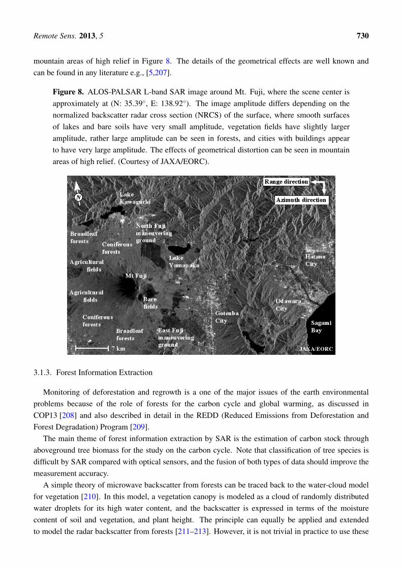
Figure 8 is an amplitude image around Mt. Fuji, Japan, acquired by ALOS-PALSAR L-band SAR.This amplitude image contains wealth of information on the scattering objects. For example, there is nobackscatter from the shadowed part in the mouth of Mt. Fuji, and the image consists of just system noise.Normalized radar cross section (NRCS) is little from dead-calm water surface of lakes and sea, because,under no wind or very low wind speed, the most of the incident microwave is reflected in the speculardirection and little is backscattered. However, NRCS increases with increasing wind speed since thesurface becomes increasingly rough. NRCS from bare soil and weed in the maneuvering grounds isslightly larger than NRCS from the water surface due to backscattering from random rough surfaces.Vegetation in agricultural fields has larger NRCS than the former areas, and NRCS from forests is verylarge. Increased NRCS from vegetation and even larger NRCS from forests are mainly caused by volumeand multiple scattering. The largest NRCS is from buildings in the cities because of multiple reflectionsbetween the ground and building walls. The very large NRCS from urban areas arises if the roads andbuilding walls are aligned orthogonal to the radar illumination direction. Thus, if the urban structures arenot in the orthogonal to the line-of-sight direction, the incident microwave does not backscatter towardthe radar antenna and the images appear dark. In order to compensate this effect, polarimetric analysescan be applied to enhance the images of urban areas [118]. Another way of compensating this effect isto use SAR images acquired from different geometries.
3.1.2. Geometrical Effects
Apart from the image amplitude modulation by the microwave scattering process, the imagemodulation by geometrical effects inherent to the side-looking radar takes an important role. Theareas surrounding Mt. Fuji are bare soil, but the face of Mt. Fuji in the radar direction appears verybright, partly because the surface is tilted toward the radar illuminating direction giving rise to increasedradar backscatter by so-called tilt modulation, and partly because of the geometrical effect known asforeshortening. The latter geometrical effect, including shadowing and layover, can be seen in the
Remote Sens. 2013, 5 730
mountain areas of high relief in Figure 8. The details of the geometrical effects are well known andcan be found in any literature e.g., [5,207].
Figure 8. ALOS-PALSAR L-band SAR image around Mt. Fuji, where the scene center isapproximately at (N: 35.39◦, E: 138.92◦). The image amplitude differs depending on thenormalized backscatter radar cross section (NRCS) of the surface, where smooth surfacesof lakes and bare soils have very small amplitude, vegetation fields have slightly largeramplitude, rather large amplitude can be seen in forests, and cities with buildings appearto have very large amplitude. The effects of geometrical distortion can be seen in mountainareas of high relief. (Courtesy of JAXA/EORC).
3.1.3. Forest Information Extraction
Monitoring of deforestation and regrowth is a one of the major issues of the earth environmentalproblems because of the role of forests for the carbon cycle and global warming, as discussed inCOP13 [208] and also described in detail in the REDD (Reduced Emissions from Deforestation andForest Degradation) Program [209].
The main theme of forest information extraction by SAR is the estimation of carbon stock throughaboveground tree biomass for the study on the carbon cycle. Note that classification of tree species isdifficult by SAR compared with optical sensors, and the fusion of both types of data should improve themeasurement accuracy.
A simple theory of microwave backscatter from forests can be traced back to the water-cloud modelfor vegetation [210]. In this model, a vegetation canopy is modeled as a cloud of randomly distributedwater droplets for its high water content, and the backscatter is expressed in terms of the moisturecontent of soil and vegetation, and plant height. The principle can equally be applied and extendedto model the radar backscatter from forests [211–213]. However, it is not trivial in practice to use these

Remote Sens. 2013, 5 731
numerical models directly to retrieve forest information and computing above-ground tree biomass, sincemany parameters, such as number of branches, orientations, and sizes, are required for computation.The practical approach is the empirical and model-based semi-empirical methods utilizing the relationbetween the SAR data and in situ sample data measured by field survey. There are four main empiricaland model-based approaches to date. The first is to use the relationship between the NRCS and biomassor stem volume, and there exist a substantial number of reports on this issue for various locationsand species [214–222] (see also a good review paper [223]). The second approach is based on SARinterferometry [224–235], (see also a recent study using UAVSAR [236]), and the third approach isbased on PolSAR and Pol-InSAR [141,144,147–150,152–156,237]. The fourth approach is to use therelation between biomass and image texture [238–243].
The method based on NRCS has been studied since 1980s. The general trend is that NRCSincreases with increasing aboveground biomass in both conifer and deciduous trees, but saturates atcertain biomass levels. This saturation biomass increases with increasing radar wavelengths. Since themicrowave of longer wavelength can penetrate deeper into forest interior, the backscattered microwavecontains more information on the forest such as branches and trunks that are the major constituents ofaboveground biomass. The dominant scatterers at X- and C-bands are the canopy layer; while those atL-band are the canopy and branches as well as the ground-volume (branches/trunks) reflection. TheP-band backscatter has similar contributions as those of L-band, but with increased ground-volumecontribution. It is also known that the cross-polarization data have higher correlation with tree biomassthan the co-polarization data. Since the present scattering theories are not practical, regression analysesare usually made using the NRCS and sample biomass data acquired by field survey, and from theregression model function the average tree biomass of forests can be estimated from the NRCS of SARdata only. The model function is not universally applicable to all types of forests, but it depends onthe forests types and locations, e.g., conifers, deciduous, broad or needle leaves, rain forests, or borealforests, and ground topography, so that the corresponding model function needs to be recalculated forthe forests of interest.
Although the topic of this section is the amplitude information, it is appropriate, at this stage, toprovide a brief account on the techniques of InSAR and Pol-InSAR for the forest information extraction.
The general approach of interferometric SAR is based on the relation of the coherence of complexinterferogram and stem volume, i.e., InSAR coherence decreases with increasing stem volume(Biomass), and also the relation of the InSAR phase with effective tree height. The coherence-basedmethod uses a semi-empirical water cloud model, and the repeat-pass InSAR coherence of a forest isconsidered as the sum of the ground and volume contributions, which are expressed in terms of stemvolume and tree height. There are several unknown parameters in this model, and they are empiricallydetermined and approximated under appropriate assumptions. The model is trained with sample dataand stem volume is estimated. For a given tree species, the stem volume is closely related to the treeheight, and biomass using allometric equations e.g., [244].
The phase-based method originates from the early study using the C-band repeat-pass ERS-1inteferometric data over boreal forests, suggesting that the coherence was high enough under stableenvironmental condition in winter to estimate the InSAR phase center (effective scattering center) whichis close to the forest height, and hence the tree height (and biomass) could be estimated [224,225].

Remote Sens. 2013, 5 732
However, Santoro et al. [233] reported that the tree height estimation by InSAR phase is less accuratethan that by InSAR coherence.
The upper limits of measurable biomass by the multi-temporal InSAR technique appear to be higherthan those of NRCS saturation biomass. However, the technique is limited by the baseline decorrelation,and environmental conditions, including wind speed, temperature, rain, and snow. The results of theC-band InSAR coherence over boreal forests suggest that the most suitable conditions for the stemvolume estimation is under stable winter conditions with a snow cover and an at least moderatebreeze [235].
The recent studies suggest that Pol-InSAR (and tomography) is an effective means of retrieving forestinformation such as tree height [141,144,147–150,152,153], and to estimate above-ground tree biomasswith increased accuracy compared with the PolSAR technique [155]. Estimated tree heights appear tobe in good agreement with lidar measurements [141,147,148,152,152,156], suggesting a potential ofcombining lidar and Pol-InSAR for forestry and related applications.
On the other hand, several reports indicate the limitation of multi-temporal Pol-InSAR and InSARmethods imposed by the temporal decorrelation caused by the environmental conditions [231,233,235],which cannot easily be quantified in terms of interferometric coherence even if the information on theseconditions are available [237].
The technique of biomass estimation by Pol-InSAR uses the Random Volume over Ground (RVoG)model which is also based on the water cloud mode. In this model, a covariance matrix is producedfrom the multiple polarimetric data sets acquired from slightly different baseline separations. Thecovariance matrix (see Equation (7) in Section 5) describes the degree of correlation between differentpolarization images that are directly related to the physical elements of scattering objects. Thiscovariance matrix is decomposed into the ground and volume contributions; the former correspondsto the surface and double-bounce scattering contributions, and the latter the scattering contribution fromvertically distributed canopy layer. In both covariance matrices, each elements (i.e., cross-covariancematrices) are proportional to the interferometric coherence or decorrelation between interferometric pairsof different baseline combinations. The forest height can be inferred from the different combinationsof interferometric coherence under the same assumptions as those for InSAR technique, where thedielectric constant of canopy layers are statistically uniform and that the volume component obeysa negative exponential function in the vertical (forest height) direction (it is based on the negativeexponential transmissibility).
The texture-based approach makes use of the non-Gaussianity of amplitude fluctuations in ahigh-resolution SAR images of forests. The principal idea of this approach is that the images of sparselydistributed trees have statistically high non-Gaussianity, and they tend to be Gaussian distributed as theforests become increasingly dense, i.e., increasing biomass. Thus, the model uses the relation betweenthe parameter(s) of the amplitude distribution function that fits best to the data and sample biomass.Wang et al. [241,242] reported that the K-distribution [238,240,245–247] is a versatile distributionfunction that describes the non-Gaussian amplitude fluctuations in the high-resolution SAR images offorests. The robust model based on the regression relation between the amplitude or intensity momentsand tree biomass does not require a distribution function [243]. Both the models have larger saturationbiomass than the NRCS model. In the texture-based technique of Wang et al. [241] and Wang and

Remote Sens. 2013, 5 733
Ouchi [242], only coniferous forests were used to test the algorithms, and thus, further studies usingdifferent types of forests are required for their validity.
It has been shown that the L-band NRCS depends also on the soil moisture [234,248]. It was foundthat the highest correlation was observed when the soil moisture was highest, that the influence of soilmoisture on NRCS was biomass dependent, and that the effect was large for smaller tree biomass for thesimple reason that the ground contribution increases with decreasing biomass. From the study over theAlaskan coniferous forests, Kasischke et al. [248] suggest that to use the L-band NRCS for the biomassestimation and monitoring forest regrowth will require development of approaches to account for thevariations of soil moisture, particularly, for the forests of low levels of aboveground biomass.
In the most studies mentioned above, the forests are located on flat ground or ground of gentleslope. In the areas of large topographic undulations or mountainous regions, there exist the effectsof foreshortening and layover, resulting in the increased NRCS and hence spurious relation between theabove ground biomass and NRCS. Thus, the removal of topographic contribution to NRCS is requiredfor such cases [207,249,250].
3.1.4. Soil Moisture
Estimation of soil moisture is one of the top-priority subjects in agriculture and in the study on theinteraction between atmosphere and land surface. Apart from the SAR parameters (radar incidenceangle, wavelength, and polarization), there are two main contribution to radar backscatter from bare soil;surface roughness and dielectric constant, the latter of which yields the soil moisture. In order to retrievethe soil moisture content, it is necessary to eliminate the contribution from surface roughness, and theproblem is ill-posed such that it is not a straightforward task from a single set of SAR data without priorknowledge. It becomes even more difficult for the fields covered by vegetation and the ploughed fieldswhich give rise to the directional and surface-tilt dependencies on microwave backscatter.
To date, three types of models for soil moisture retrieval have been proposed: physical-basedtheoretical model, semi-empirical model, and empirical model. In the physical-based model, the NRCSis computed using scattering theories that take into account the dielectric constant of the scatteringsurface [251] (see also [252]). The generally used theory is the integral equation model (IEM) firstdeveloped by Fung et al. [253], which is based on the combination of the Kirchhhoff or physicaloptics model (KM, POM) [254] and the small perturbation model (SPM) [255,256]. In principle, theformer is applicable to the surface (single-bounce) scattering from the perfectly conducting surface andis independent of polarization. The latter is polarization-dependent and is a function of the dielectricconstant of the scattering media of slightly rough surface. Although improved IEM [257,258] and severaldifferent approximations [259–262] (see also a recent comprehensive book by Fung and Chen [263])have been proposed, it is rather difficult to estimate soil moisture from theoretical models alone withoutprior knowledge such as surface roughness, and it is rarely used in practice.
Empirical models such as those of [264–266] are based on the empirical relation between the NRCSand soil moisture, and as such, they are site-limite, dependent on radar parameters and surface roughness,and require a large amount of datasets. The empirical models can be useful for the areas where sampledata are collected, but they are not, in principle, applicable to other sites.
Remote Sens. 2013, 5 734
Semi-emperical models overcome the difficulty of the theoretical models by combining thescattering theories and empirical models [267–270], which do not require prior information on surfaceroughness [271]. The model developed by Oh et al. [267,270] appears to be most widely used. In thismodel, the ratio of σHH/σV V and that of σHV /σV V are expressed as functions of the Fresnel reflectioncoefficient and surface roughness, where σmn is the NRCS of mn polarization with m,n = H,V . Sincethere are two functions (polarization ratios) and two unknown parameters (dielectric constant and surfaceroughness), the dielectric constant and hence soil moisture can be estimated by solving these twoequations with the empirical datasets of different polarizations. This model, therefore, requires fullypolarimetric data.
The semi-empirical model of Dubois et al. [268] uses the functional expressions for σHH and σV V interms of dielectric constant and surface roughness for specific radar parameters, and thus, requiring onlythe dual-polarization data sets. While, the model of Shi et al. [269] is based on the regression analysisof simulation of the IEM at a single polarization.
Numerous experimental studies have been reported on the soil moisture retrieval by active microwavesensors since mid 1970s, some of which agree and some disagree with the theoretical models andsemi-empirical models. Examples include those of [272–282]. See also the techniques based on DInSARdata [283], CP-SAR data [135], PolSAR data [284], and the combination of optical with SAR data [285]and with PolSAR data [286]. For further details, please see the special issues on SMEX 2004 (SoilMoisture Experiments 2004) [287] and Retrieval of Bio- and Geophysical Parameters from SAR Datafor Land Applications [288]; also the operational performance [289]. An excellent and comprehensivereview article with extensive reference papers by Brian et al. [290] is also available.
It may be of some interest, although SAR sensors are not onboard, that the SMOS (Soil Moisture andOcean Salinity) mission [291–293] was launched in 2009 to provide maps of soil moisture and oceansalinity by a passive L-band 2-dimensional microwave interferometric radiometer which is the first of itskind in the spacebone platform.
3.1.5. Vegetation
Another important topic in the field of agriculture is monitoring of staple foods such as rice, maze,wheat, and soybeans. Since rice, among those staple foods, is the major staple food for over the halfthe world population, monitoring of rice ecosystems by SAR is briefly described here as an example.On this topic, substantial numbers of studies have been reported to date using the test sites mainly inAsia [120,294–315].
From those studies, it is understood that the microwave backscatter at high frequencies such as K- toX-bands from rice fields is dominated by canopy scattering, while the microwave at lower frequenciessuch as L-band has contributions both from canopy and soil or water surface (when irrigated) due tolonger penetration depth. The general trend of the temporal variation of NRCS from rice fields is thatthere is a certain amount of backscatter from bare soil before irrigation, and the NRCS drops to almost asystem noise level after irrigation due to specular reflection by water surface. The area of rice plantation,and possibly yields, can be estimated from this information. The NRCS increases with the growth ofcrops, and the decreases slightly in the heading stage.

Remote Sens. 2013, 5 735
From the theoretical point of view, the temporal and spatial variations of NRCS can be computed byusing models based on the radiative transfer theory [294,297]. However, due to the local variation andcomplexity of the theory, the empirical approach based on the regression analysis of NRCS and in situdata on the rice fields is generally used to monitor the rice ecosystems.
Measurements based on a multifrequency polarimetric scatterometer indicate that the backscatteringcoefficients of the high frequency bands (K- to X-bands) correlated poorly with LAI (leaf area index)and biomass of rice plants, while LAI is best correlated with the backscattering coefficients of C-bandHH- and HV-polarizations, and the biomass is best correlated with those of L-band HH-polarization data.SAR measurements also showed that C-band HV-polarization data have a significant correlation with thedevelopment of rice plants [314,315]. In general, C-band microwave backscatter seems to show goodcorrelation with rice plants with high signal-to-noise ratio (SNR), and it is also suggested the HH/VVpolarization ratio is a useful parameter for monitoring rice during growing season and classification ofrice and non-rice fields [308,309]. Similarly, a recent study using TerraSAR-X data showed a significantcorrelation of the X-band HH/VV ratio with the development of rice plants [313]. At L-band, it wasreported that little radar backscatter from rice fields was observed in JERS-SAR and airborne Pi-SARL-band data, and occasionally it yielded the Bragg resonant backscatter from regularly planted bunchesof rice plants [301,305,307]. A recent report [311], however, showed some promise of utilizing L-bandHV-polarization data by avoiding the Bragg scattering. Wang et al. [310] also showed the possibleuse of PALSAR L-band HH-polarization data that are sensitive to the structure of rice plants thanVV-polarization data. Polarimetric analyses have been studied for the application to rice monitoring,and Li et al. [120] concluded that the Touzi decomposition [108] is best for classification of rice fields,requiring only a single date of imagery. Based on the analyses of RADARSAT-2 quad-polarizationdata, Wu et al. [314] suggested a good set of parameters to classify rice fields are those at HH- andHV-polarizations, and HH/VV ratio.
3.1.6. Other Land Features
Measurement of surface topography by radar is generally made by InSAR (see Section 4and references therein). Another technique is radargrammetry [316–319] which is based on thephotogrammetry utilizing the parallax of stereoscopic pairs of images of a same area acquired withtwo different viewing angles. The main difference between the two approaches is that the parallaxmeasurements are made using the phase difference in InSAR and amplitude in radargrammetry.Radargrammetry has been used for producing the surface relief of the planet Venus by the S-bandMagellan-SAR [320–322] and Earth by RADARSAT [323] with recent examples by TerraSAR-X [324],Cosmo-SkyMed [325], and the combination of the both [326]. These techniques require multiple setsof complex (InSAR) or amplitude (radargrammetry) SAR data. While, radarclinometry [327–333],based on the optical shape-from-shading [334], uses only a single SAR image to estimate local terrainslope by inversion of the radiometric incidence angle correction. Radarclinometry originates fromphotoclinometry (see [328] and references therein), and has been studied in the field of computervision [335]. Radarclinometry using SAR data was first proposed by Wildey [327,328] for producinglandscapes of Venus by the Venera-15 [336], where stereoscopic SAR data were not available. Sinceradarclinometry relies on the relation between the image intensity (or amplitude) and local surface
Remote Sens. 2013, 5 736
slope, modeling of intensity distribution is crucial. The Lambertian model, generally used in thephotoclinometry [334], assumes a random rough and statistically uniform surface yielding the imageintensity proportional to the cosine of the local tilt angle. However, this model is not generallyapplicable to SAR data, and various distribution functions have been used to model SAR image statistics,including Gaussian [329,337], Rayleigh [338], Gamma [339,340], and Rayleigh-Bessel composite [332]distributions (see also [238]). Radarclinometry is simple and easy to implement, but the technique isconsidered as a qualitative relief reconstruction method for its accuracy is marred by large errors causedby the geometric effect of foreshortening and speckle noise [333].
Amplitude data can be applied to monitoring and estimation of parameters of other land featuresincluding those listed in Table 1. The progress and present status in these fields of applications can befound in recent journals and proceedings (e.g., [341–344]). Note that the aforementioned referencescontain SAR applications to land surfaces using not only amplitude information but also applications toother fields such as oceanography, as well as technology and methodology.
3.2. Oceanic Features
The research and development on SAR applications to oceanography are matured to a certain level,and a large number of papers and documentations are available elsewhere (see, for example, [345,346],and the proceedings on ESA documents from the series of SEASAR Workshop [347–350]).
3.2.1. Scattering from Sea Surface
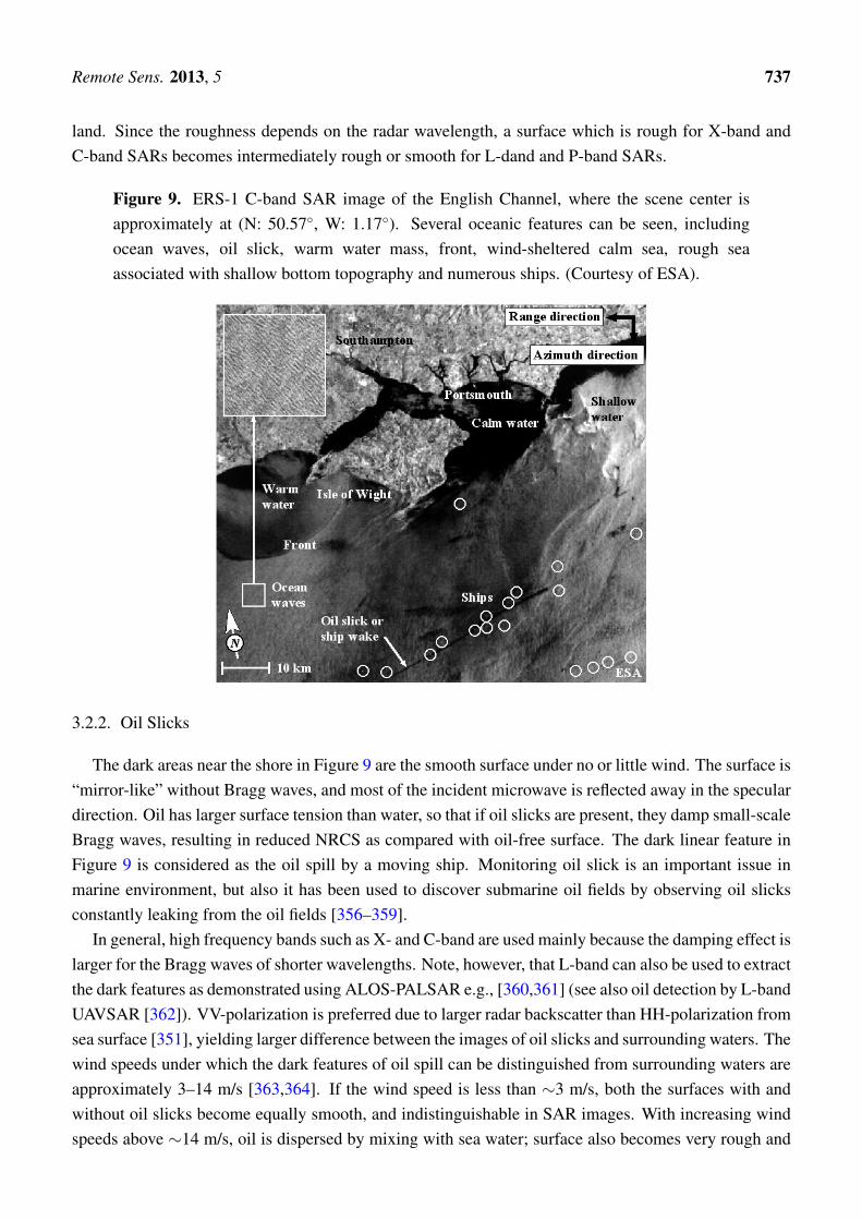
Figure 9 is the ERS-1 C-band SAR image of the English Channel. The microwave backscatteringprocess from sea surface is predominantly surface scattering (apart from volume scattering from formsand sprays, and man-made targets such as vessels), and NRCS depends on surface roughness anddielectric constant of the water, e.g., [345,351,352]. The elementary scatterers are small-scale waveswhose wavelength satisfies the Bragg resonance condition, LBragg = λ/(2 sin θi), where LBragg is thewavelength of small-scale waves, λ is the radar wavelength and θi is the incidence angle. It may beof historic interest, but as the name suggests, the Bragg resonance scattering was first discovered byBragg in the X-ray diffraction from crystals in 1913 [353,354]. It was 42 years later in 1955 that thephenomenon of the Bragg scattering in the microwave backscatter from the sea surface was first foundby Crombie [355]. There are numerous experimental evidence to support the theory of Bragg waves asthe main elementary scatterers on the sea surface. Temporal and spatial changes of the Bragg wavescaused by, for example, ocean waves, internal waves, and ocean wind, modulate the radar backscatter,and thus, these oceanic features can be made visible in SAR images.
At this stage, the criterion of surface roughness is introduced. The criterion, whether a surface isrough or smooth, is dependent on the radar wavelength and incidence angle. According to the Rayleighcriterion, the surface is considered as rough yielding large radar backscatter if the standard deviation σHof vertical undulation is large compared to the reference roughness λ/(8 cos θi), the surface is moderatelyrough and smooth if σH is comparable with and much smaller than the reference roughness respectively(σH should not be confused with NRCS σHH,V V,HV ). This criterion applies any surface over water and
Remote Sens. 2013, 5 737
land. Since the roughness depends on the radar wavelength, a surface which is rough for X-band andC-band SARs becomes intermediately rough or smooth for L-dand and P-band SARs.
Figure 9. ERS-1 C-band SAR image of the English Channel, where the scene center isapproximately at (N: 50.57◦, W: 1.17◦). Several oceanic features can be seen, includingocean waves, oil slick, warm water mass, front, wind-sheltered calm sea, rough seaassociated with shallow bottom topography and numerous ships. (Courtesy of ESA).
3.2.2. Oil Slicks
The dark areas near the shore in Figure 9 are the smooth surface under no or little wind. The surface is“mirror-like” without Bragg waves, and most of the incident microwave is reflected away in the speculardirection. Oil has larger surface tension than water, so that if oil slicks are present, they damp small-scaleBragg waves, resulting in reduced NRCS as compared with oil-free surface. The dark linear feature inFigure 9 is considered as the oil spill by a moving ship. Monitoring oil slick is an important issue inmarine environment, but also it has been used to discover submarine oil fields by observing oil slicksconstantly leaking from the oil fields [356–359].
In general, high frequency bands such as X- and C-band are used mainly because the damping effect islarger for the Bragg waves of shorter wavelengths. Note, however, that L-band can also be used to extractthe dark features as demonstrated using ALOS-PALSAR e.g., [360,361] (see also oil detection by L-bandUAVSAR [362]). VV-polarization is preferred due to larger radar backscatter than HH-polarization fromsea surface [351], yielding larger difference between the images of oil slicks and surrounding waters. Thewind speeds under which the dark features of oil spill can be distinguished from surrounding waters areapproximately 3–14 m/s [363,364]. If the wind speed is less than ∼3 m/s, both the surfaces with andwithout oil slicks become equally smooth, and indistinguishable in SAR images. With increasing windspeeds above ∼14 m/s, oil is dispersed by mixing with sea water; surface also becomes very rough and
Remote Sens. 2013, 5 738
the dumping effect becomes negligible. Oil dispersion is also caused by dissolution, oxidization, andbiodegradation. Thus, with increasing time from the oil discharge and with increasing wind speed, oilslicks become undetectable. The time that takes oil to disperse varies from day to weeks, depending onseveral factors such as the types of oil, amount of discharge, and meteorological conditions.
The main problem in the detection of oil slick features is to separate the dark features causedby oil slick from other look-alikes such as calm sea surfaces, rain cells, upwelling, and biogenicslicks [365,366]. If oil is discharged from a moving ship, a linear dark oil trail appears in SAR images,but the shapes of slicks become complex if the oil is discharged from a maneuvering ship and strongnon-uniform currents are present [367].
Several approaches have been proposed to solve this problem, including the algorithms based onneural network and fuzzy logic [368–376]. A recent study proposed a trained one-class classificationapproach [377] which appeared superior over the two-class classification algorithms such as those basedon neural network. Further advances have been made recently using polarimetric analysis [378–380]. Forfurther details, see comprehensive review articles with extensive reference papers by Topouzelis [381]and by Leifer et al. [382].
There are several operational systems for oil slick detection by SAR, such as GNOME (GeneralNOAA Operational Modeling Environment) [383] and ISTOP (Integrated Satellite Tracking ofPolluters) [384,385].
3.2.3. Ocean Winds
The wind-dependent radar backscatter as seen in Figure 9 is the basis of estimating the wind speedover the oceans. There are two approaches to the wind speed measurements by SAR. The first approachutilizes the standard algorithm based on the empirical geophysical model function (GMF) used in themicrowave wind scatterometers [8,386–389]. There are well-defined GMFs at Ku-band to L-band, inparticular, the Ku- and C-band GMFs are very accurate for the reasons that these bands are generallyused for wind scatterometers [390]. The function relates NRCS at different incidence angles to thewind speeds (10 m above the sea surface) and wind directions with respect to the line-of-sight direction.The technique requires a precise radiometric calibration of the SAR image, and the estimation accuracydecreases with increasing wind speeds.
The second approach is based on the azimuth cut-off (or correlation) algorithm [391–393]. As willbe described in the following section of ocean waves, the SAR image spectrum of a two-dimensionalwave field is constrained in the azimuth direction by the non-linear image modulation process of oceanwaves, and the smallest measurable wavelength, that is, the cut-off wavelength, is dependent on the windand sea state conditions, where the relation can be described by a quasi-linear ocean-to-SAR transformmodel [394]. Based on this rationale, a semi-emperical model was developed to estimate the wind speedfrom the azimuth cut-off wavelength without requiring the wind direction and precise calibration ofNRCS [391–393]. Although further validation tests are required, the model appears to show sufficientaccuracy under some limited conditions.
Wind speed can be measured from SAR data, but, unlike scatterometers that use multiple beams atdifferent look angles, the direction cannot be estimated directly by the single-beam SAR. In general,wind directions are estimated by other sources such as inter-look cross-spectra [395], wind streaks in
Remote Sens. 2013, 5 739
SAR images [396–398], and polarimetric analysis [399,400]. The SAR-based wind data are used tofill the gap in the scatterometer data [401–405], and to study climate, atmosphere-ocean interaction andextreme events such as hurricanes and cyclones [406–408]. They are also used in coastal zones wherethe measurements are difficult to make by wind scatterometers of low spatial resolution ranging fromseveral kilometers to few tens of kilometers. One of the interesting applications of SAR-based wind datais the search for suitable areas for constructing offshore wind farms [409–411].
3.2.4. Ocean Waves
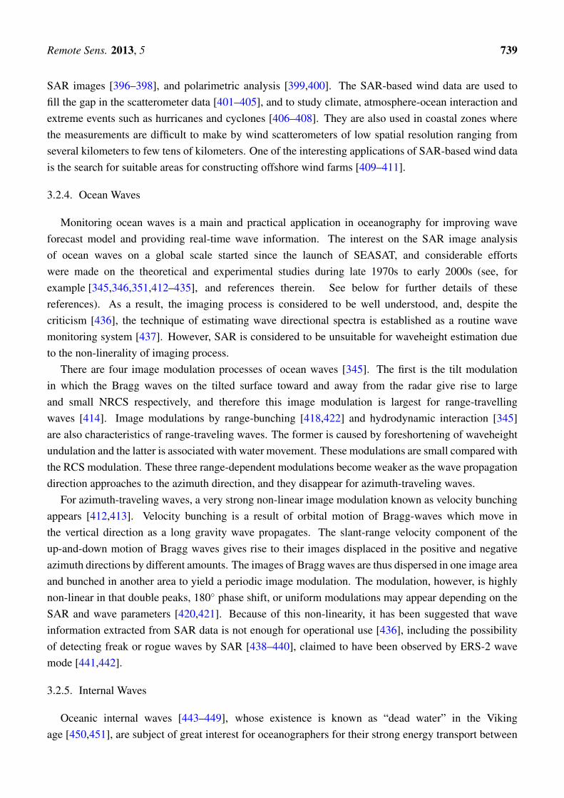
Monitoring ocean waves is a main and practical application in oceanography for improving waveforecast model and providing real-time wave information. The interest on the SAR image analysisof ocean waves on a global scale started since the launch of SEASAT, and considerable effortswere made on the theoretical and experimental studies during late 1970s to early 2000s (see, forexample [345,346,351,412–435], and references therein. See below for further details of thesereferences). As a result, the imaging process is considered to be well understood, and, despite thecriticism [436], the technique of estimating wave directional spectra is established as a routine wavemonitoring system [437]. However, SAR is considered to be unsuitable for waveheight estimation dueto the non-linerality of imaging process.
There are four image modulation processes of ocean waves [345]. The first is the tilt modulationin which the Bragg waves on the tilted surface toward and away from the radar give rise to largeand small NRCS respectively, and therefore this image modulation is largest for range-travellingwaves [414]. Image modulations by range-bunching [418,422] and hydrodynamic interaction [345]are also characteristics of range-traveling waves. The former is caused by foreshortening of waveheightundulation and the latter is associated with water movement. These modulations are small compared withthe RCS modulation. These three range-dependent modulations become weaker as the wave propagationdirection approaches to the azimuth direction, and they disappear for azimuth-traveling waves.
For azimuth-traveling waves, a very strong non-linear image modulation known as velocity bunchingappears [412,413]. Velocity bunching is a result of orbital motion of Bragg-waves which move inthe vertical direction as a long gravity wave propagates. The slant-range velocity component of theup-and-down motion of Bragg waves gives rise to their images displaced in the positive and negativeazimuth directions by different amounts. The images of Bragg waves are thus dispersed in one image areaand bunched in another area to yield a periodic image modulation. The modulation, however, is highlynon-linear in that double peaks, 180◦ phase shift, or uniform modulations may appear depending on theSAR and wave parameters [420,421]. Because of this non-linearity, it has been suggested that waveinformation extracted from SAR data is not enough for operational use [436], including the possibilityof detecting freak or rogue waves by SAR [438–440], claimed to have been observed by ERS-2 wavemode [441,442].
3.2.5. Internal Waves
Oceanic internal waves [443–449], whose existence is known as “dead water” in the Vikingage [450,451], are subject of great interest for oceanographers for their strong energy transport between

Remote Sens. 2013, 5 740
continental shelf and deep water, their effects on phytoplankton and fishery, and the effects on ships,submarines, marine architecture, oil platforms, underwater communications, and sonar, as well as theeffects on underwater workers. A comprehensive report on the oceanic internal waves is available withthe principles and examples in [452]. Internal waves are generated at the boundary of a stratified waterlayers, e.g., light (warm or low saline) water on top of dense (cold or high saline) water. When thisboundary is disturbed by ships, submarines, or the interaction between current and bottom topography,internal waves are produced on the boundary. As the waves propagate, the water particles take circularmotion, and this motion in the upper water layer gives rise to converging and diverging surface currents.The surface of current convergence becomes rough, while that of diverging current becomes smooth.These smooth and rough surfaces can be imaged by SAR as a manifestation of internal waves [453].The another mechanism is the dumping of small-scale waves by surface films in the current convergencezone which appear dark in SAR images [454–457].
Internal waves appear either as solitary waves (solitons) or a wave packet containing multiples ofwaves of increasing wavelength with increasing distance from the source of wave generation. Unlikeocean surface waves of wavelengths up to several hundreds of meters, the wavelengths of internal wavesrange from hundreds of meters to tens of kilometers with phase velocities from about 0.1 m/s to severalm/s with periods ranging from several minutes to several hours, and propagate long distance.
The general theoretical interpretation is based on the non-linear Korteweg-De Vries (K-dV) equationthat describes the interface displacement between the two layers in terms of phase velocity, non-linearcoefficient, and dispersion coefficient [458,459]. The K-dV equation, under certain conditions, has ananalytical solution that describes nonlinear solitary internal waves (solitons) in the water of constantdepth [460,461]. The amplitude, phase velocity of solitons, and horizontal velocities of water particlescan then be calculated. Because of the nonlinear nature of the K-dV equation, its solutions andapproximations under different conditions have been a subject of much interest in the fields ofmathematics and nonlinear studies as well as fluid dynamics. The modified K-dV equation takes intoaccount the effects of water depth and nonuniform medium, which can also be used to simulate theevolution of internal waves [462–470].
Given the spatial and temporal variations of the surface current induced by the internal wave, thechanges of surface waves can be approximated by using the action balance equation [471–474] thatdescribes the waveheight spectrum in terms of the varying surface current, wind speed and direction.Scattering models such as POM is then used to compute the NRCS from the water surface perturbed bythe interaction of surface waves and currents [475–477].
Observations of internal waves by optical sensors onboard aircrafts and satellites were reported inthe 1950s to 1970s [478,479], and by airborne SARs [480]. Research of internal waves by spaceborneSAR was initiated again by the launch of SEASAT in 1978. Since then numerous studies have beenreported on the naturally occurring internal waves often observed at the boundaries of deep waters andcontinental shelfs as a result of current-botoom interaction e.g., [481–493], as well as ship-generatedinternal waves [494–498]. Detection of submarines by SAR has interested military sectors for over 20years [454], but no clear evidence of detection ability has been reported to date.
Remote Sens. 2013, 5 741
3.2.6. Bottom Topography
The shallow waters in Figure 9 have large radar backscatter because the surface is rough caused bythe interaction of currents and bottom topography. The image amplitude has strong correlation withbottom topography [499–503], and using this relation, attempts have been made to map the depth ofcoastal waters [504]. A general approach is to measure first the depths at several reference points byother instruments like acoustic sensors, and using these depths as calibration data the contours of depthare computed from NRCS. The effect of bottom topography to the surface currents appears to be limitedto the waters of depth less than approximately 30–40 m. The shallow waters in Figure 9 ranges from2–33 m according to the sea chart.
3.2.7. Fronts
The linear feature of oceanic fronts between the warm water mass and cold water is known as thethermal front. Fronts are often associated with fisheries and the data can be used to locate good fishingwaters around the oceanic fronts. SAR can be a suitable sensor to locate oceanic fronts for its all-weatherand day-and-night observation ability [505–510]. Monitoring warm and cold waters, major currents andfronts can also be made by optical and thermal sensors, and thus, complementary use of these sensorscan be a possible future approach to increase the detection accuracy and information content in the data.
3.2.8. Ship Detection and Identification
Ship detection and identification by airborne radar were the major issue during the World War II, butthe research on ship detection by spaceborne SAR started when SEASAT was launched in 1978 [511].Since then a substantial number of papers and review articles have been published, including thoseof [512–532], and also good review articles are available [533–536].
The reasons for the active research on ship detection are due to the increasing international maritimeproblems and requirements, such as monitoring of maritime traffic and fishing activity, tracking andidentifying illegally operating ships, ships intruding into territorial waters, those responsible for oil spill,and surveillance of piracy [537].
At present, AIS (Automatic Identification System) is mandatory to all passenger ships and shipsover 300 tonnage cruising international waters. In the European Union, VMS (Vessel MonitoringSystem) is mandatory to all fishing boats longer than 15 m. AIS and VMS are the systems for cruisingships and monitoring stations to exchange information on their positions, types, nationalities, cruisingspeeds and directions through direct or through satellite communications. The conventional AIS systemuses ground-based monitoring stations, so that AIS signals can be received from only ships within50–70 km from coasts. In order to extend the AIS signal reception on a global scale, some commercialsatellite-borne AIS systems are being operated [538,539], and real-time vessel positions and informationare available online [540]. However, small boats and illegally operating ships are not equipped AIS/VMStransponders, and in order to detect and identify these vessels, development of vessel detection systemsincorporating spaceborne and airborne SARs has been in progress.
Algorithms for ship detection include the amplitude based Constant False Alarm Rate(CFAR) which is the standard and most widely used algorithm [541–543], multi-look

Remote Sens. 2013, 5 742
cross-correlation [515,525], along-track InSAR [521,527], polarimetric analysis (with and withoutCFAR) [516,518,523,524,526,528,529,531,532], and others (see review papers [533–536] forfurther information).
The progress of ship identification by SAR is rather slow in comparison with that of ship detectiondue mainly to low resolution of spaceborne SAR. Indeed, the DECLIM report in 2006 stated “Toderive a vessel’s type (tanker, fishing boat, etc.) is beyond today’s capabilities” [519]. However,with increasing maritime problems by vessels and increasing SAR resolution in recent years, needhas been raised by coast guards and related organizations for ship identification, which initiated theresearch and development of integrated ship detection and identification systems. There are threemain approaches to ship identification: (1) Decision-based classification [544–546]; (2) Classificationby pattern matching [547]; and (3) Multi-channel classification [516,548–552], excluding the use ofISAR (Inverse SAR) [553]. Probably, the most practical algorithm at present may be the decision-basedclassification by GMV Aerospace and Defense in Spain [546].
Currently, AIS/VIS with SAR has been used in practice by several European and Canadiancommunities. For example, MARISS (Maritime Security Services) by ESA/NASA/JPL covers the northAtlantic sea to east-Atlantic sea as well as Baltic and Mediterranean seas [554]. Others include theMEOS SAR Ship Detection system by Kongsberg Spacetec (Norway) [555], SIMONS (Ship MonitoringSystem) developed by GMV Aerospace, S.A. [556], DECLIM (Detection and Classification of MaritimeTraffic from Space) project by Joint Research Center (JRC) [514,517,519,520], and that by DefenceResearch and Development Canada [557]. These commercial and institutional systems also includealgorithms for oil spill monitoring. Further details can be found in the corresponding websites.
4. Interferometry
The concept of interferometric SAR, which is the microwave version of optical holographicinterferometry [558–560], was first applied to the planet Venus [561] and later Moon [562,563] bythe ground-based radars of MIT Lincoln Laboratory operating at 7.84 GHz (wavelength 3.83 cm) onEarth (termed as “delay-doppler method”). Its application to Earth was first suggested by Graham in1974 [47], and the practical study on SAR interferometry started in 1980s, with the pioneering studyusing the airborne JPL SAR (currently AIRSAR) data by Zebker and Goldstein [564] followed bySIR-B data [565], and those of SEASAT-SAR [566,567]. Unlike the techniques using amplitude dataor polarimetry, SAR interferometry can provide strictly quantitative measurements. Although there issome space for basic research such as phase unwrapping, the InSAR technology is now almost at acomplete stage and has been used as a practical tool. The principle of InSAR is to extract quantitativeinformation on the scattering objects from complex interferograms produced by two or more sets ofmutually correlated complex SAR images of a same scene. There are two types of InSAR depending onmeasurable quantities. The first is CT-InSAR including DInSAR (Differential InSAR) [48,51–53], andthe second is AT-InSAR e.g., [63,71] as illustrated in Figure 10. The details of these systems are beyondthe scope of this article, but brief summaries are presented as follows.
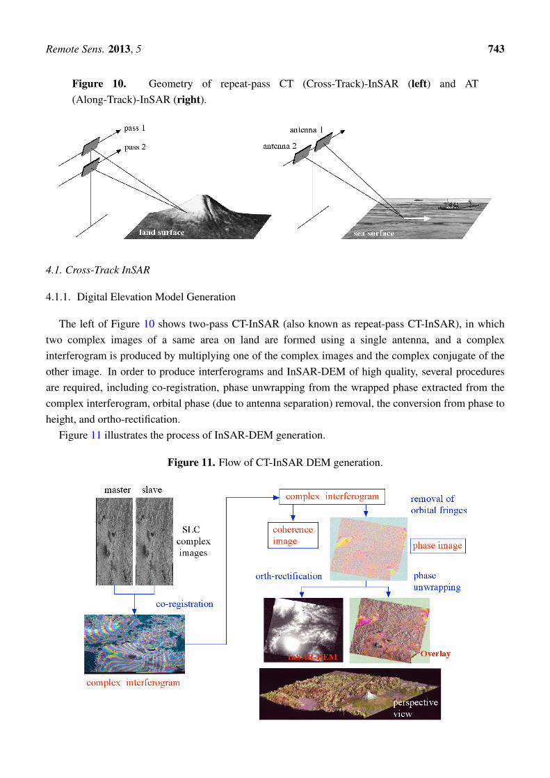
Remote Sens. 2013, 5 743
Figure 10. Geometry of repeat-pass CT (Cross-Track)-InSAR (left) and AT(Along-Track)-InSAR (right).
4.1. Cross-Track InSAR
4.1.1. Digital Elevation Model Generation
The left of Figure 10 shows two-pass CT-InSAR (also known as repeat-pass CT-InSAR), in whichtwo complex images of a same area on land are formed using a single antenna, and a complexinterferogram is produced by multiplying one of the complex images and the complex conjugate of theother image. In order to produce interferograms and InSAR-DEM of high quality, several proceduresare required, including co-registration, phase unwrapping from the wrapped phase extracted from thecomplex interferogram, orbital phase (due to antenna separation) removal, the conversion from phase toheight, and ortho-rectification.
Figure 11 illustrates the process of InSAR-DEM generation.
Figure 11. Flow of CT-InSAR DEM generation.
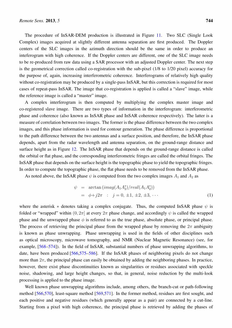
Remote Sens. 2013, 5 744
The procedure of InSAR-DEM production is illustrated in Figure 11. Two SLC (Single LookComplex) images acquired at slightly different antenna separation are first produced. The Dopplercenters of the SLC images in the azimuth direction should be the same in order to produce aninteferogram with high coherence. If the Doppler centers are different, one of the SLC image needsto be re-produced from raw data using a SAR processor with an adjusted Doppler center. The next stepis the geometrical correction called co-registration with the sub-pixel (1/8 to 1/20 pixel) accuracy forthe purpose of, again, increasing interferometric coherence. Interferograms of relatively high qualitywithout co-registration may be produced by a single-pass InSAR, but this correction is required for mostcases of repeat-pass InSAR. The image that co-registration is applied is called a “slave” image, whilethe reference image is called a “master” image.
A complex interferogram is then computed by multiplying the complex master image andco-registered slave image. There are two types of information in the interferogram: interferometricphase and coherence (also known as InSAR phase and InSAR coherence respectively). The latter is ameasure of correlation between two images. The former is the phase difference between the two compleximages, and this phase information is used for contour generation. The phase difference is proportionalto the path difference between the two antennas and a surface position, and therefore, the InSAR phasedepends, apart from the radar wavelength and antenna separation, on the ground-range distance andsurface height as in Figure 12. The InSAR phase that depends on the ground-range distance is calledthe orbital or flat phase, and the corresponding interferometric fringes are called the orbital fringes. TheInSAR phase that depends on the surface height is the topographic phase to yield the topographic fringes.In order to compute the topographic phase, the flat phase needs to be removed from the InSAR phase.
As noted above, the InSAR phase ψ is computed from the two complex images A1 and A2 as
ψ = arctan (imag(A1A∗2)/real(A1A
∗2))
= ϕ+j2π : j = 0, ±1, ±2, ±3, · · · (1)
where the asterisk ∗ denotes taking a complex conjugate. Thus, the computed InSAR phase ψ isfolded or “wrapped” within (0, 2π] at every 2π phase change, and accordingly ψ is called the wrappedphase and the unwrapped phase ϕ is referred to as the true phase, absolute phase, or principal phase.The process of retrieving the principal phase from the wrapped phase by removing the 2π ambiguityis known as phase unwrapping. Phase unwrapping is used in the fields of other disciplines suchas optical microscopy, microwave tomography, and NMR (Nuclear Magnetic Resonance) (see, forexample, [568–574]). In the field of InSAR, substantial numbers of phase unwrapping algorithms, todate, have been produced [566,575–586]. If the InSAR phases of neighboring pixels do not changemore than 2π, the principal phase can easily be obtained by adding the neighboring phases. In practice,however, there exist phase discontinuities known as singularities or residues associated with specklenoise, shadowing, and large height changes, so that, in general, noise reduction by the multi-lookprocessing is applied to the phase image.
Well known phase unwrapping algorithms include, among others, the branch-cut or path-followingmethod [566,570], least-square method [569,571]. In the former method, residues are first sought, andeach positive and negative residues (which generally appear as a pair) are connected by a cut-line.Starting from a pixel with high coherence, the principal phase is retrieved by adding the phases of
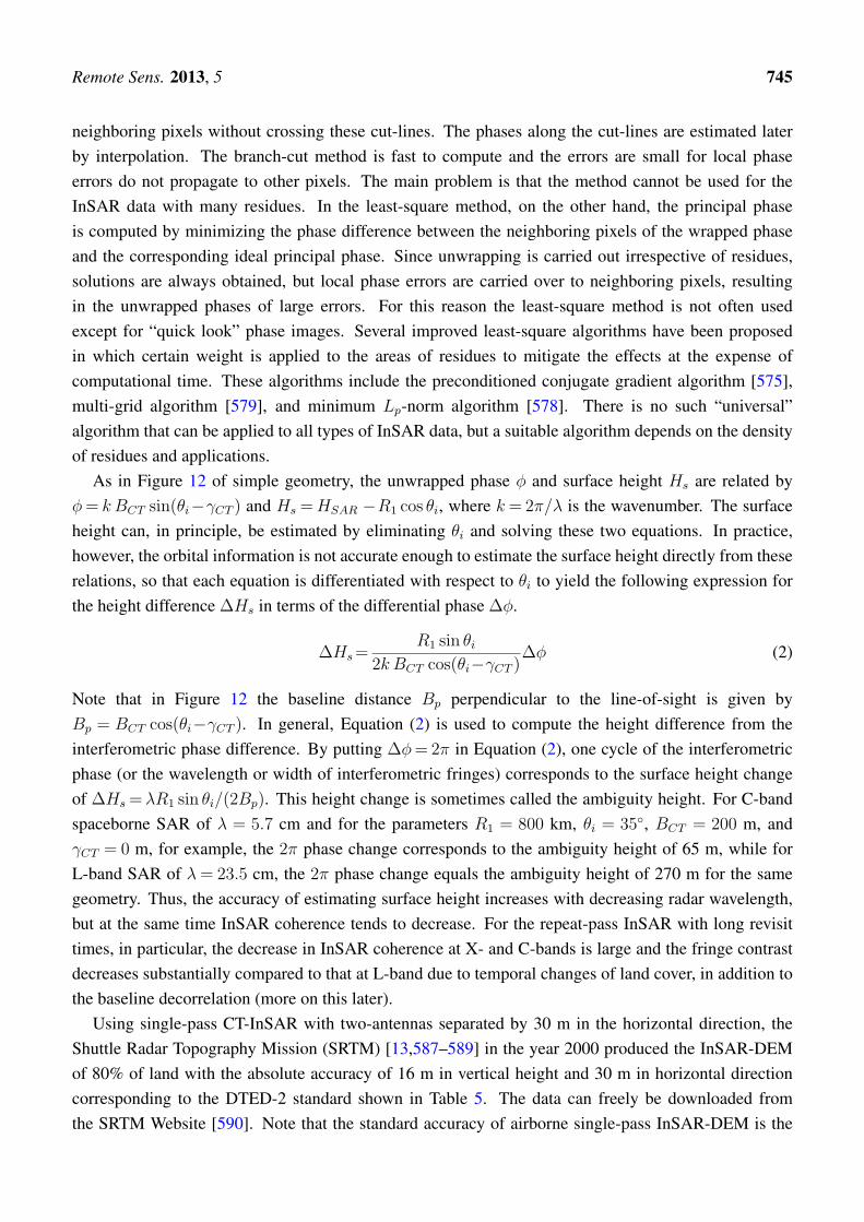
Remote Sens. 2013, 5 745
neighboring pixels without crossing these cut-lines. The phases along the cut-lines are estimated laterby interpolation. The branch-cut method is fast to compute and the errors are small for local phaseerrors do not propagate to other pixels. The main problem is that the method cannot be used for theInSAR data with many residues. In the least-square method, on the other hand, the principal phaseis computed by minimizing the phase difference between the neighboring pixels of the wrapped phaseand the corresponding ideal principal phase. Since unwrapping is carried out irrespective of residues,solutions are always obtained, but local phase errors are carried over to neighboring pixels, resultingin the unwrapped phases of large errors. For this reason the least-square method is not often usedexcept for “quick look” phase images. Several improved least-square algorithms have been proposedin which certain weight is applied to the areas of residues to mitigate the effects at the expense ofcomputational time. These algorithms include the preconditioned conjugate gradient algorithm [575],multi-grid algorithm [579], and minimum Lp-norm algorithm [578]. There is no such “universal”algorithm that can be applied to all types of InSAR data, but a suitable algorithm depends on the densityof residues and applications.
As in Figure 12 of simple geometry, the unwrapped phase ϕ and surface height Hs are related byϕ= k BCT sin(θi−γCT ) and Hs =HSAR −R1 cos θi, where k= 2π/λ is the wavenumber. The surfaceheight can, in principle, be estimated by eliminating θi and solving these two equations. In practice,however, the orbital information is not accurate enough to estimate the surface height directly from theserelations, so that each equation is differentiated with respect to θi to yield the following expression forthe height difference ∆Hs in terms of the differential phase ∆ϕ.
∆Hs=R1 sin θi
2k BCT cos(θi−γCT )∆ϕ (2)
Note that in Figure 12 the baseline distance Bp perpendicular to the line-of-sight is given byBp = BCT cos(θi−γCT ). In general, Equation (2) is used to compute the height difference from theinterferometric phase difference. By putting ∆ϕ=2π in Equation (2), one cycle of the interferometricphase (or the wavelength or width of interferometric fringes) corresponds to the surface height changeof ∆Hs = λR1 sin θi/(2Bp). This height change is sometimes called the ambiguity height. For C-bandspaceborne SAR of λ = 5.7 cm and for the parameters R1 = 800 km, θi = 35◦, BCT = 200 m, andγCT = 0 m, for example, the 2π phase change corresponds to the ambiguity height of 65 m, while forL-band SAR of λ= 23.5 cm, the 2π phase change equals the ambiguity height of 270 m for the samegeometry. Thus, the accuracy of estimating surface height increases with decreasing radar wavelength,but at the same time InSAR coherence tends to decrease. For the repeat-pass InSAR with long revisittimes, in particular, the decrease in InSAR coherence at X- and C-bands is large and the fringe contrastdecreases substantially compared to that at L-band due to temporal changes of land cover, in addition tothe baseline decorrelation (more on this later).
Using single-pass CT-InSAR with two-antennas separated by 30 m in the horizontal direction, theShuttle Radar Topography Mission (SRTM) [13,587–589] in the year 2000 produced the InSAR-DEMof 80% of land with the absolute accuracy of 16 m in vertical height and 30 m in horizontal directioncorresponding to the DTED-2 standard shown in Table 5. The data can freely be downloaded fromthe SRTM Website [590]. Note that the standard accuracy of airborne single-pass InSAR-DEM is the
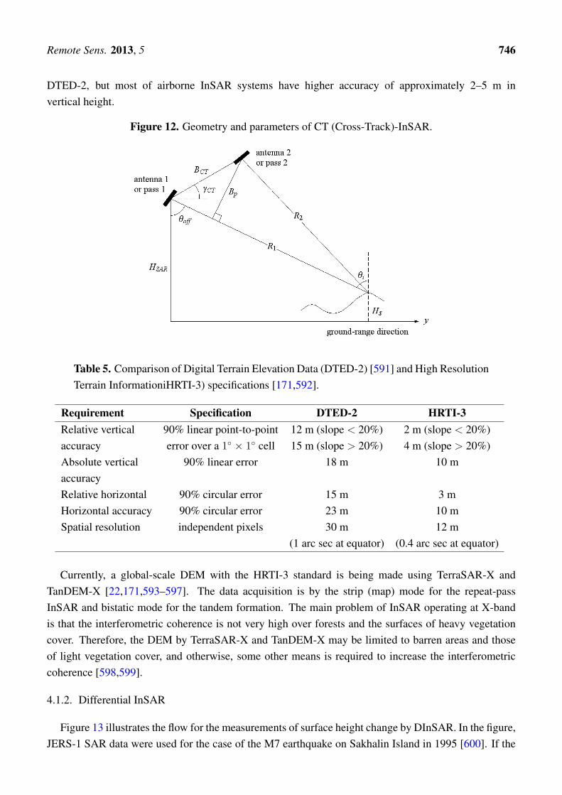
Remote Sens. 2013, 5 746
DTED-2, but most of airborne InSAR systems have higher accuracy of approximately 2–5 m invertical height.
Figure 12. Geometry and parameters of CT (Cross-Track)-InSAR.
Table 5. Comparison of Digital Terrain Elevation Data (DTED-2) [591] and High ResolutionTerrain InformationiHRTI-3) specifications [171,592].
Requirement Specification DTED-2 HRTI-3Relative vertical 90% linear point-to-point 12 m (slope < 20%) 2 m (slope < 20%)accuracy error over a 1◦ × 1◦ cell 15 m (slope > 20%) 4 m (slope > 20%)Absolute vertical 90% linear error 18 m 10 maccuracyRelative horizontal 90% circular error 15 m 3 mHorizontal accuracy 90% circular error 23 m 10 mSpatial resolution independent pixels 30 m 12 m
(1 arc sec at equator) (0.4 arc sec at equator)
Currently, a global-scale DEM with the HRTI-3 standard is being made using TerraSAR-X andTanDEM-X [22,171,593–597]. The data acquisition is by the strip (map) mode for the repeat-passInSAR and bistatic mode for the tandem formation. The main problem of InSAR operating at X-bandis that the interferometric coherence is not very high over forests and the surfaces of heavy vegetationcover. Therefore, the DEM by TerraSAR-X and TanDEM-X may be limited to barren areas and thoseof light vegetation cover, and otherwise, some other means is required to increase the interferometriccoherence [598,599].
4.1.2. Differential InSAR
Figure 13 illustrates the flow for the measurements of surface height change by DInSAR. In the figure,JERS-1 SAR data were used for the case of the M7 earthquake on Sakhalin Island in 1995 [600]. If the
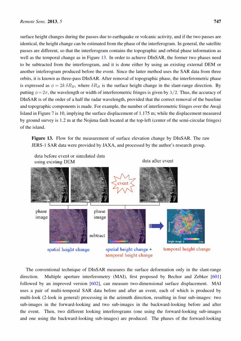
Remote Sens. 2013, 5 747
surface height changes during the passes due to earthquake or volcanic activity, and if the two passes areidentical, the height change can be estimated from the phase of the interferogram. In general, the satellitepasses are different, so that the interferogram contains the topographic and orbital phase information aswell as the temporal change as in Figure 13. In order to achieve DInSAR, the former two phases needto be subtracted from the interferogram, and it is done either by using an existing external DEM oranother inteferogram produced before the event. Since the latter method uses the SAR data from threeorbits, it is known as three-pass DInSAR. After removal of topographic phase, the interferometric phaseis expressed as ϕ = 2k δRH , where δRH is the surface height change in the slant-range direction. Byputting ϕ=2π, the wavelength or width of interferometric fringes is given by λ/2. Thus, the accuracy ofDInSAR is of the order of a half the radar wavelength, provided that the correct removal of the baselineand topographic components is made. For example, the number of interferometric fringes over the AwajiIsland in Figure 7 is 10, implying the surface displacement of 1.175 m; while the displacement measuredby ground survey is 1.2 m at the Nojima fault located at the top-left (center of the semi-circular fringes)of the island.
Figure 13. Flow for the measurement of surface elevation change by DInSAR. The rawJERS-1 SAR data were provided by JAXA, and processed by the author’s research group.
The conventional technique of DInSAR measures the surface deformation only in the slant-rangedirection. Multiple aperture interferometry (MAI), first proposed by Bechor and Zebker [601]followed by an improved version [602], can measure two-dimensional surface displacement. MAIuses a pair of multi-temporal SAR data before and after an event, each of which is produced bymulti-look (2-look in general) processing in the azimuth direction, resulting in four sub-images: twosub-images in the forward-looking and two sub-images in the backward-looking before and afterthe event. Then, two different looking interferograms (one using the forward-looking sub-imagesand one using the backward-looking sub-images) are produced. The phases of the forward-looking
Remote Sens. 2013, 5 748
and backward-looking interferograms are proportional to the forward-looking and backward-lookingdisplacements respectively. Subtraction of these phases, therefore, yields the surface displacement in theazimuth direction. Bechor and Zebker [601] tested the algorithm using ERS-2 C-band SAR data over theHector Mine earthquake in 1999, and compared with with GPS and offset-derived displacements data,resulting in the accuracy of 3–11 cm for coherence 0.8–0.4. The technique has been used by severalresearchers for the measurements of surface deformation by the 2003 Mw7.2 Altai earthquake [603],and seismic analyses e.g., [604,605].
4.1.3. Atmospheric and Ionospheric Effects
Occasionally, a phenomenon associated with microwave propagation delay caused by spatial andtemporal atmospheric variations in the troposphere is observed [606–609], in particular, in DInSARphase images. As in Figure 12, InSAR and DInSAR techniques are based on the measurements oftwo-way path difference ∆R = 2(R1 −R2) in a radar wavelength scale. If microwave pulses passthrough locally dense vapor in the troposphere, there appears a time delay caused by the vapor, andthe path difference becomes ∆R+∆RT where ∆RT is the path difference corresponding to this timedelay [610,611]. The path difference ∆RT may be as large as tens of centimeters in spatial scale [608],and therefore, the interferometric phase corresponding to this delay causes erroneous measurements ofsurface topography or deformation [612,613]. It is common to separate the tropospheric delays into twocomponents: one related to turbulent mixing processes and the other related to tropospheric stratification.
The phase delay associated with the atmospheric turbulence can be corrected or mitigated by stackingor averaging a large number of interfetograms, since the turbulence has short spatial correlation lengthwith virtually no temporal correlation between data acquisition times e.g., [608,614–616]. Troposphericstratification is associated with temperature, pressure, and water vapor, and it introduces phase delayscorrelated with topography, leading to misinterpreted InSAR data in the areas of steep topographye.g., [617]. To correct these effects, stacking of multiple interferograms is not, in general, successful,due to the periodic nature of the perturbation in the interferometric phase. Several correction methodshave been proposed, including those utilizing external independent data such as local atmosphericmodels [618], GPS (Ground Positioning System) [619–621], spaceborne optical data [622,623], a stackof small baseline SAR interferograms [624,625], and a multi-scale time-series approach [626]. Amongthose, an approach utilizing global scale atmospheric models appears very promising [627,628]. It wasalso suggested that the removal of the atmospheric effects before phase unwrapping reduces the errorsin phase unwrapping in the areas of high relief [628]. For further details, see a good review article onthe issue of atmospheric effects and their mitigation [612,613].
Spatial and temporal variations of electron density in the ionosphere have a significant impact onSAR, InSAR, and DInSAR as well as PolSAR [629–631]. The effects of ionospheric delays becomesignificant at lower frequencies, since the variance of the refractive index fluctuations is approximatelyproportional to λ4, as observed in the RADARSAT C-band and JERS-1 L-band SAR amplitude imagesover the auroral zones in Alaska, showing kilometer-scale linear or banding patterns in the azimuthdirection, termed as “azimuth streaks” [632]. The effects of ionospheric fluctuation have been observednear the magnetic poles [632,633], particularly during strong magnetic disturbances, but also in the areasaway from the polar regions, such as the ALOS-PALSAR L-band data over Japan and Brazil [634], and
Remote Sens. 2013, 5 749
the 2008 Sichuan Earthquake [635,636]. In addition to azimuth streaks, ionospheric delays caused bythe variations of total electron content (TEC) introduce Faraday rotation (see the polarization paragraphsin Section 1 and references therein), relative range delay between interferometric data acquisition times,range and azimuth defocusing, loss of interferometric coherence, and phase errors. Azimuth streaks andrange shifts cause misregistration in the subpixel correlation in both the azimuth and range directions ininterferometry, and decorrelation as reported in the study on the 2008 Sichuan Earthquake [635].
Due to the dispersive nature, the effects of ionospheric delays can, in principle, be separated fromnon-dispersive features of surface deformation and atmosphere. The range split-spectrum method [637]is based on this separation of dispersive and non-dispersive effects on the InSAR phase [638]. In thismethod, the range spectrum of an InSAR dataset is split into two parts of high and low frequencysub-bands, and each part is used to form an inteferogram. Assuming that the two interferograms have thesame non-dispersive effects with different dispersive contributions depending on the inter-band centerfrequency, the relative TEC can be estimated by subtracting the phases of these interferograms. Thesplit-spectrum method, however, can estimate only the relative values of TEC but not the absolute values.
Matter and Gray [639] suggested a method of estimating and reducing the effect of azimuth streakson the InSAR phase from a map of azimuth offset. Improved versions [635,636] have been proposedbased on the relation between the ionospheric contributions to the azimuth offset and interferometricphase derived by Mayer et al. [640,641]. From this relation the interferometric phase errors causedby the spatial variation of TEC, i.e., azimuth streaks, can be estimated empirically using the azimuthoffset values [639] and removed, enhancing surface topography and coseismic deformation measures.Another technique is based on Faraday rotation. The angle of Faraday rotation can be measured fromfully polarimetric data [642,643]. Then from the relation of the rotation angle and TEC [128] (andwith known SAR geometry), 2-dimensional distribution of TEC and hence maps of phase delay can beestimated [633,644].
These observations of atmospheric and ionospheric effects, on the other hand, may lead to newtechniques to study the high-resolution troposphere turbulence and stratification and TEC by InSARand DInSAR.
4.1.4. Examples of DInSAR Applications
The first experimental result of DInSAR was reported by Gabriel et al. [52] using the SEASAT-SARdata, detecting small elevation change caused by increased soil moisture by irrigation in the agriculturalarea of California. The first DInSAR measurements of crustal movement by earthquakes were madeusing the ERS-1 SAR data over the Landers earthquake, California in 1992 [645–647]; and the firstmeasurement of glacier flow in Antarctica by the JPL group [648]. These early studies initiated thestudy on geodetic dynamics by DInSAR that followed.
Examples of DInSAR measurements of deformation by earthquakes also include the 1994 Northridgeearthquake in California [649], the Great Hanshin-Awaji earthquake, Japan in 1995 [650] also shown inFigure 7, the Sichuan earthquake, China [651], the L’Aquila earthquake, Italy both in 2009 [652], andthe recent Tohoku-Oki earthquake in 2011 [653,654].
Surface deformation by volcanic activity was reported, such as the case of Kilauea volcano, Hawaii bySIR-C data [655] and the discovery of fore active volcanoes in the central Andes mountains previously
Remote Sens. 2013, 5 750
considered to be dormant using ERS-1 and ERS-2 data [656]. Other applications include landslideand subsidence monitoring [657,658], surface deformation by constructing dams [659], undergroundexcavations [660,661] and by groundwater extraction [662–664], and topographic changes and flow ofglaciers [665–669]. Examples and details on the InSAR and related techniques can be found in the ESAwebsite [670], and also the selected papers of the ESA Fringe 2007 Workshop a special issue of Journalof Applied Geophysics [671].
4.1.5. PS-InSAR
PS-InSAR was developed by Politechnico di Milano (Italy) in 2000 [54–56,59]. In 2003, GAMMAREMOTE SENSING (Switzerland) developed a similar software Interferometric Point Target Analysis(IPTA) combined with Persistent Scatterer InSAR [58]. A similar algorithm known as InSAR CTM(Coherent Target Monitoring) [57,60] was developed by Vexcel Corp. (currently in Microsoft Corp.),and also CPT (Coherent Pixels Technique) by the Universitat Politecnica de Catalunya, Spain [61].
The principle of PS-InSAR is to measure the phase difference of particular point-like targets whichyield consistent strong backscatter over a year or years. In general, at least 10–20 image sets arerequired to achieve PS-InSAR. Stacks of multi-temporal SAR data mitigate the phase distortion causedby atmospheric effect. The accuracy of estimating surface height deformation is of the order of fewmillimeters per year (see also [54–62]). Stacking of multiple interferograms has also been used forconventional DInSAR. An example is SBAS (small baseline subset) InSAR [624,625] which uses onlyinterferograms produced with short baseline separation in order to reduce both spatial and temporaldecorrelation, and mitigate atmospheric effects and topographic errors.
Examples of PS-InSAR include the measurements of subsidence by groundwater extraction,underground mining, and tunneling of underground railways [672–675]. PS-InSAR is very accurate andeffective in urban areas where many point-like targets exist, but not effective in natural fields withoutmany permanent (or persistent) scatterers. For such cases, several corner reflectors can be deployed assemi-permanent scatterers.
Recently, a new algorithm termed as “SqueeSAR” was proposed to utilize not only permanent(deterministic) scatterers but also distributed scatterers using their statistical property [676]. Thealgorithm is capable of measuring surface deformation over non-urban areas of sparsely distributeddeterministic scatterers. Prior to SqueeSAR, another (free) software package “StaMPS (StanfordMethod for Persistent Scatters)” was developed [677]. As for SqueeSAR, StaMPS can be applied topersistent scatterers as well as distributed scatterers by incorporating the small baseline and persistentscatterer methods.
4.1.6. Ground-Based InSAR
The principle of the ground-based InSAR is the same as that of multi-temporal InSAR and DInSARfor generating DEM [678–681], and measurements of small surface movement [682–684]. Insteadof airborne or spaceborne SARs, the system consists of (X-band in general) T/R horn antennasfixed on a platform that slides along the horizontal axis to achieve aperture synthesis. Targetsof ground-based DInSAR are generally sloped surfaces which are suspected to subside, and many
Remote Sens. 2013, 5 751
differential interferograms are made over a certain period of time, depending the magnitude ofmovement. The fixed rail on which the platform slides is considered as stationary during the observation,otherwise motion compensation is required. The system has been used to monitor the subsidence ofcliffs over which an ancient monument is standing, and suspected subsidence and hazardous areas. Notethat a recent work showed that a ground-based real-aperture radar can as well be effective for DEMgeneration [685].
4.1.7. Interferometric Coherence
Another property of complex interferograms is the interferometric coherence or degree of correlationdefined as
Γ12=|⟨A1A
∗2⟩|√
⟨I1⟩⟨I2⟩(3)
where ⟨ ⟩ indicates taking an ensemble average, and Ij=AjA∗j (j=1, 2) is the intensity. In practice, the
ensemble average is replaced by a sample average over finite pixels. If the coherence is low, the contrastof interferometric fringes becomes low, or even no fringes are produced. The areas of no interferometricfringes in the complex interferogram in Figure 11 correspond to those of little coherence. In repeat-passInSAR and DInSAR, the SAR antenna illuminates a scattering object at different incidence angles andat different times, resulting in decrease in coherence. The InSAR coherence is composed of a product offour main contributions as follows.
Γ12=ΓN · ΓT · ΓB · ΓS. (4)
ΓN is the loss of coherence by the additive system noise, which is not dominant if the signal-to-noiseratio (SNR) is sufficiently large. ΓN defines the maximum limit of coherence that can be achieved by theinterference of two complex images.
ΓT is the temporal decorrelation due to the interaction of the incident microwave with the scatteringobjects. This coherence loss includes the decorrelation by the temporal changes of scattering objects andthe volume (multiple) scattering associated with different incidence angles. For example, the surface ofwater changes between passes and hence the coherence over the water surface is theoretically zero (in realdata, it is non-zero due to statistical averaging). On the other hand, the surface of a solid ground does not,in general, change significantly, so that the coherence is very high. Vegetation and forests have moderateto low coherence due to volume scattering. As to the dependence of radar wavelength on ΓT , theX- and C-band radar backscatter from forests and vegetation are predominantly from the crown parts thatare susceptible to changes, and hence the temporal coherence takes small values. While, the backscatterof longer wavelengths (L- and P-bands) is mainly from stable ground, branches, and trunks, penetratingvegetation cover, and therefore, higher temporal coherence than X- and C-band can be obtained. Thesefactors causing the temporal decorrelation are the random changes of the backscattered fields (and hencethe speckle patterns) between the data takes, arising from the changes in the shapes of surfaces for thecase of surface scattering. In optical speckle interferometry, it is known as “speckle boiling” [686–688].
ΓB is the decorrelation caused by the baseline separation. Higher interferometric coherencecan be obtained with shorter baseline separation, but at the expense of interferometric resolution.As in Equation (2) and discussion with it, the ambiguity height is inversely proportional to the
Remote Sens. 2013, 5 752
baseline separation, and hence the accuracy of height measurements decreases with decreasing baselineseparation. A good measure for the limit of baseline separation is known as the critical baseline(separation) BC
p defined as the distance with which the corresponding interference fringes are resolved,i.e., fringe separation equals the spatial resolution cell. Then, assuming ρR as the slant-range resolutioncell, the critical baseline is defined, by setting ∆H = ρR cos θi and ∆ϕ = 2π in Equation (2), asBC
p = λR1 tan θi/(2ρR). For C-band spaceborne SAR of λ = 5.7 cm, R1 = 800 km, θi = 35◦, andρR =25 m, the critical baseline is BC
p ≃ 0.64 km. For L-band SAR of λ=23.5 cm, BCp ≃ 2.6 km for
the same geometry and resolution.ΓS describes the coherence as a function of surface slope. With reference to Figure 12, if a flat
surface is tilted toward the radar at an angle θS , the effective incidence angle becomes (θi−θS), andhence BC
p = λR1 tan(θi−θS)/(2ρR). Thus, the critical baseline becomes smaller, and the coherencedecreases. For the surface tilted away from the radar, the reverse process increases the coherence.Another simple way to look at this effect is the width (or wavelength) of interferometric fringes, given byλR1 tan(θi−θS)/(2BCT ), where γCT =0 is assumed for simplicity. It can be seen that the fringe widthdecreases as the tilt angle θS increases. It means that the ”effective” baseline separation increases, andtherefore, the coherence decreases. For the surface tilted away from the radar, the fringe width increases,so that the effective baseline separation decreases to yield higher interferometric coherence. It shouldbe mentioned that higher interferometric coherence can be gained by increasing off-nadir (incidence)angles, but at the expense of reduced NRCS, i.e., reduced SNR.
It can further be noticed that the fringe width increases as the radar wavelength λ increases, and theaccuracy of height estimation decreases as also mentioned with reference to the ambiguity height andEquation (2). On the other hand, the interferometric coherence increases with increasing λ since thecritical baseline increases. There is a trade-off between the interferometric coherence and the accuracyof height measurements. Although X- and C-band SARs are useful for DEM generation (and indeed isbeing in progress using TerraSAR-X and TanDEM-X [22,171,593–597]), L-band SAR has an advantagefor its high coherence over the surfaces covered by vegetation and insensitivity to the changes over longtime periods, in particular, for the measurements of temporal surface height changes by DInSAR.
In DInSAR, smaller or ideally no baseline separation is desirable to reduce the baseline decorrelationΓB in Equation (4). The effects of SNR and surface slope on the coherence are the same as for InSARdescribed above. The effect of volume scattering in the temporal decorrelation ΓT is also the same.Another factor which causes the temporal decorrelation is the amount of surface displacement. If asurface translates or changes its height due, for example, to earthquakes, in such a way that the phasechanges more than one cycle within the slant-range resolution cell, then interference does not occur. Thiscritical displacement in the slant-range distance corresponds to δRH=λ/2. The equivalent phenomenonhas been known in optical speckle interferometry as “speckle translation” [688,689].
It is of some interest that for large translation such as glacier flows and large deformation byearthquakes or volcanic activity, the conventional DInSAR cannot be applied due to the loss of coherenceby speckle translation. In such cases, a technique called “speckle-tracking” (also called “sub-pixel imagecorrelation”) is often used [690–694]. It is a kind of pattern matching, in which the patch of a samespeckle image is sought between two SAR images and a flow vector is produced, provided that there is nospeckle boiling. This subject matter may belong to amplitude information in Section 3, but a brief note is

Remote Sens. 2013, 5 753
given here for the sake of continuity. The second approach to tackle large deformation was the two-stephybrid algorithm based on a rubber-sheeting coregistration to improve interferometric coherence andrange offset image subtraction to mitigate steep phase gradient [695]. Unlike the conventiona methodsof InSAR, the rubber-sheeting coregistration is a non-parametric method, in which a slave image isprojected on a rubber sheet which is overlaid with a master image. Then, the slave image is distortedto match the features of the master image. A range offset image is then produced, smoothed, andsubtracted from the interferogram before phase unwrapping. Finally,the interferogram is unwrapped,and the offset field is added back to recover the true phase. Using ENVISAT-ASAR data over theGalapagos Islands, Yun et al. [695] retrieved an interferogram inside the caldera of an erupted volcano,which other conventional InSAR algorithms could not.
As mentioned in the forestry application of Section 3.1.3, InSAR coherence has some correlation withtree biomass to yield the coherence-based biomass retrieval algorithm [225,226,228,229,231,235].
4.2. Along-Track InSAR
The geometry of AT-InSAR is shown in Figure 10. AT-InSAR consists of two (or more) antennasplaced along the body of an aircraft platform, and can measure the range velocity component of movingscatterers [63–72]. In general, a forward (or aft) antenna transmits signals and return signals are recivedby both antennas. If the scatterers have a slant-range velocity component vR, the signals received by thetwo antennas have different Doppler centers, and the phase difference is given by ψ = k tBvR, wheretB = BAT/V is the time lag between the two antennas separated by the distance BAT , and V is theplatform velocity.
The system was limited to the airborne platform due to technical difficulty. In 2000, however, anexperimental AT-InSAR was carried out by Shuttle-borne SRTM. SRTM was designed originally forCT-InSAR with two antennas separated by 60 m in the cross-track direction, but in addition, theywere separated by 7 m in the along-track direction. Further, TerraSAR-X has two antennas split inthe along-track direction to experiment AT-InSAR from space for ocean current measurements [73]. Themeasurement accuracy of SRTM AT-InSAR is approximately 0.2 m/s [70], and the accuracy of 0.1 m/s isexpected by TerraSAR-X. In 2009, TanDEM-X, identical to TerraSAR-X, was launched, and AT-InSARby the formation flight is one of the secondary mission objectives [22].
The interferometric coherence is another aspect of AT-InSAR. In the same way as for CT-InSAR, thecoherence decreases with increasing baseline separation (or time-lag tB); while increasing tB increasesinterferometric phase ψ and hence increases the measurement accuracy. Thus, there is a trade-offbetween the accuracy of estimating InSAR phase (and hence velocity) and coherence. In general, theinterferometric phase of AT-InSAR does not exceed 2π for the case of ocean currents, so that phaseunwrapping is not required. The measurement accuracies of airborne AT-InSAR are few centimetersper second, depending on the radar wavelength and antenna separation. The interferometric coherenceis also a function of the time duration (surface coherence time) over which the principal scatterers, i.e.,Bragg waves, retain the same shape. Longer the wavelength of ocean waves is, longer the coherence timebecomes. For AT-InSAR operating at X- to L-bands, the coherence time is estimated as approximately0.2–0.02 ms [65,66,696–699].
Remote Sens. 2013, 5 754
As mentioned briefly in Section 2.3, the conventional AT-InSAR system with two antennas measuresonly the velocity in the range direction, while an airborne AT-InSAR equipped with four antennas wasdeveloped to produce current vectors [71].
AT-InSAR can also detect and measure the slant-range velocity of a moving hard targets such asvehicles and ships [74–79]. The principle of this technique known as moving target indicator (MTI)by AT-InSAR is essentially the same as that for current measurements. It utilizes the difference in theinterferometric phase between a moving hard target and a stationary target, in that the velocity andacceleration components in the azimuth and range directions give rise to the phase difference to thereturn signals.
5. Polarimetry
SAR polarimetry is a current “hot topic”. Expectation of polarimetry to extend the currentSAR and InSAR technologies has lead increasing number of spaceborne SARs equipped with thequad-polarimeric mode as listed in Table 2 and almost all airborne SARs are able to acquirequad-polarization data. This enthusiasm stems from the fact that polarimetric data contain moreinformation on the scattering objects than the conventional single- and dual-polarization data. PolSARdata describe the changes of polarization states of received microwave by the structures and dielectricconstants of the objects, so that these properties can, in principle, be extracted from the polarimetricdata. However, at present, SAR polarimetry and possible applications need further stringent validationusing ground-truth data, and it has not yet been used in practice as much as the DEM generation andmeasurements of surface deformation by SAR interferometry.
5.1. Principle of Polarimetry
A part of the reason for slow development of PolSAR in routine practice may be its mathematicalcomplexity in comparison with SAR interferometry. Much of PolSAR data analysis is based on thematrix manipulation, so that it deters researchers in some fields of geoscience and related applications,who are not accustomed to using complex matrix manipulation. Reflecting this, a free software isprovided by ESA to promote and expand the utilization of PolSAR data [700]. In the following, theprinciples of PolSAR are briefly summarized with least mathematics.
Polarimetric SAR measures the complex scattering matrix of a scattering object with differentpolarizations. On the linear polarization base, the microwave pulses of alternating horizontal and verticalpolarizations are transmitted from either a single antenna or multiple antennas, and the horizontal andvertical polarization components of the backscattered signals are received. There are four possiblecombinations of transmitted and received polarizations, i.e., HH: horizontal transmission and reception,HV: horizontal transmission and vertical reception, VV: vertical transmission and vertical reception, andVH: vertical transmission and horizontal reception. The scattering matrix [S] describes this relation ofthe polarization states before and after the microwave scattering by the objects, and is expressed by Er
H
ErV
=[S]
EtH
EtV
= SHH SHV
SV H SV V
EtH
EtV
(5)
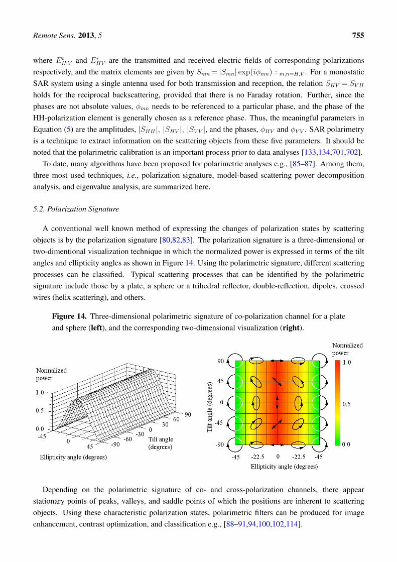
Remote Sens. 2013, 5 755
where EtH,V and Er
HV are the transmitted and received electric fields of corresponding polarizationsrespectively, and the matrix elements are given by Smn = |Smn| exp(iϕmn) : m,n=H,V . For a monostaticSAR system using a single antenna used for both transmission and reception, the relation SHV = SV H
holds for the reciprocal backscattering, provided that there is no Faraday rotation. Further, since thephases are not absolute values, ϕmn needs to be referenced to a particular phase, and the phase of theHH-polarization element is generally chosen as a reference phase. Thus, the meaningful parameters inEquation (5) are the amplitudes, |SHH |, |SHV |, |SV V |, and the phases, ϕHV and ϕV V . SAR polarimetryis a technique to extract information on the scattering objects from these five parameters. It should benoted that the polarimetric calibration is an important process prior to data analyses [133,134,701,702].
To date, many algorithms have been proposed for polarimetric analyses e.g., [85–87]. Among them,three most used techniques, i.e., polarization signature, model-based scattering power decompositionanalysis, and eigenvalue analysis, are summarized here.
5.2. Polarization Signature
A conventional well known method of expressing the changes of polarization states by scatteringobjects is by the polarization signature [80,82,83]. The polarization signature is a three-dimensional ortwo-dimentional visualization technique in which the normalized power is expressed in terms of the tiltangles and ellipticity angles as shown in Figure 14. Using the polarimetric signature, different scatteringprocesses can be classified. Typical scattering processes that can be identified by the polarimetricsignature include those by a plate, a sphere or a trihedral reflector, double-reflection, dipoles, crossedwires (helix scattering), and others.
Figure 14. Three-dimensional polarimetric signature of co-polarization channel for a plateand sphere (left), and the corresponding two-dimensional visualization (right).
Depending on the polarimetric signature of co- and cross-polarization channels, there appearstationary points of peaks, valleys, and saddle points of which the positions are inherent to scatteringobjects. Using these characteristic polarization states, polarimetric filters can be produced for imageenhancement, contrast optimization, and classification e.g., [88–91,94,100,102,114].
Remote Sens. 2013, 5 756
5.3. Model-Based Scattering Power Decomposition Analysis
In 1998, Freeman and Durden [98] proposed a three-component scattering power decompositionanalysis based on fitting the observed scattering matrix to the model-based matrix. In this analysis,the total received power P is considered as a sum of the three types of scattering powers, namely, thoseby single-bounce surface scattering, double-bounce scattering, volume (multiple) scattering as follows.
P = |SHH |2+2|SHV |2+|SV V |2=Ps+Pd+Pv (6)
where Ps, Pd, and Pv are the scattering powers by single-bounce, double-bounce, and volume scatteringsrespectively. Single-bounce surface scattering arises from the water and ground surfaces where the Braggscattering is dominant. Double-bounce scattering arises from dihedrals, for example, to wall-groundand tree trunk-ground interactions. Volume scattering can be caused by randomly orientated dipolessuch as tree branches and vegetation. Later, Yamaguchi et al. [104] extended the analysis to afour-component-scattering power decomposition by adding helix scattering. For simplicity, only thethree-component scattering power decomposition analysis is briefly described in the following.
From Equation (5), the covariance ⟨SmnS∗m′n′⟩: m,n,m′n′!H,V of different polarization combinations can
be estimated. The three- (and four-) component scattering powers are computed from the covariance orcoherency matrices. The three-component decomposition analysis assumes the reflection symmetry ofthe polarimetric covariance matrix elements, i.e., the co- and cross-polarized scattering coefficients arestatistically uncorrelated, so that the assumption of ⟨SHHS
∗HV ⟩ ≃ ⟨SV V S
∗HV ⟩ ≃ 0 holds. The reflection
symmetry occurs, for example, in L- and P-band data from forests where the phases of SHHS∗HV and
SV V S∗HV are random and uniformly distributed between (0, 2π].
The HV-base scattering matrix in Equation (5) can be represented by the covariance matrix
⟨[C]⟩=
⟨|SHH |2⟩ ⟨
√2SHHS
∗HV ⟩ ⟨SHHS
∗V V ⟩
⟨√2SHV S
∗HH⟩ ⟨2|SHV |2⟩ ⟨
√2SHV S
∗V V ⟩
⟨SV V S∗HH⟩ ⟨
√2SV V S
∗HV ⟩ ⟨|SV V |2⟩
(7)
The covariance matrix is simple and describes correlation between different polarization images that aredirectly related to the physical elements of scattering objects. Note that Equation (7) is often normalizedby the HH-polarization element as ⟨[C]⟩/⟨|SHH |2⟩.
In order to deduce the individual scattering power contributions, the scattering matrix of Equation (5)is first rotated by an angle around the radar line-of-sight direction, and expressions correspondingto the scattering elements of the covariance matrix of Equation (7) are calculated by assuming asuitable probability density function (PDF) for the orientation angles of elementary scatterers. In thethree-component decomposition analysis, this PDF is assumed to be uniform. From comparison ofthe covariance matrix elements of Equation (7) and those derived from the scattering matrix under thereflection symmetry, the following set of equations can be derived.
⟨|SHH |2⟩= |b|2fs+|a|2fd+fv⟨|SHV |2⟩=fv/3⟨SV V |2⟩=fs+fd+fv⟨SHHS
∗V V ⟩=bfs+afd+fv/3 (8)
Remote Sens. 2013, 5 757
where fs, fd, and fv are the surface, double-bounce and volume scattering contributions respectively,and a and b are unknown parameters.
The volume scattering contribution fv can be estimated directly from ⟨|SHV |2⟩ in the second ofEquation (8), so that there remain three equations and four unknown parameters. Equation (8) cannotbe solved unless one of the unknown parameters is known. An assumption is then made that if the realcomponent of ⟨SHHS
∗V V ⟩ is positive, the surface scattering is dominant and put a = −1; but if it is
negative, the double-bounce scattering is dominant and put b = 1. Once the values of a, b, fs, and fdare known, the powers, Ps, Pd, and Pv corresponding respectively to the surface, double-bounce, andvolume scattering can be estimated from
Ps=fs(1+|b|2)Pd=fd(1+|a|2)Pv=8fv/3=8⟨|SHV |2⟩ (9)
The three-component scattering decomposition assumes the reflection symmetry [98]. Thisassumption is generally valid for natural targets such as forests and vegetation, but it is often violated forurban scenes where, for example, the double-reflection scattering from the ground-building orientatedin non-orthogonal directions to the radar line-of-sight. The generalized four-component scatteringdecomposition analysis is valid without the assumption of the reflection symmetry and includes the helixscattering [104]. Helix scattering changes the linearly polarized incidence microwave to a circularlypolarized backscattered wave. This change in polarization state may be caused by, for example,crossed wires and quarter wave plates. In the four-component approach, the modified PDF takesinto account the vertical structures of tree trunks and branches and also vegetation, depending on the⟨|SHH |2⟩/⟨|SV V |2⟩ ratio.
Figure 15 shows the L-band and X-band Pi-SAR images decomposed into three scatteringpowers [305,307]. The area (the Kojima district in Okayama, Japan) is covered predominantly by ricepaddies. The image size is approximately 3.5 km in both the azimuth (from top to bottom) and range(from right to left) directions. The bunches of rice plants were mechanically transplanted in a regularinterval, and almost fully grown with height approximately 60–90 cm at the data acquisition date of the13th of July 1999.
At L-band, double-bounce scattering can be seen between roads and houses, and canal water andbanks. The dominant backscattering by double-bounce appears in the triangular district at the center ofthe image, where the walls of the houses, roads and canals that are orthogonal to the range (illumination)direction, but little double bounce scattering can be observed in other districts, where they are notnon-orthogonal to the range direction. Double-bounce scattering as a result of the Bragg resonancescattering between the bunches of rice plants and water is indicated in red in the ground survey mapin the top-left of Figure 15 [307]. Apart from the Bragg scattering, little radar backscatter is observedfrom other rice paddies due to long penetration depth of L-band microwave. Lotus plants of heightapproximately 1.5–2 m over the water indicate a mixture of double-bounce and volume scattering.Volume scattering is mainly from trees and bushes, and interestingly from vegetation in the green housescomposted of frames of metal pipes covered by polyolefin films that are transparent to microwave.

Remote Sens. 2013, 5 758
Figure 15. Airborne Pi-SAR X-band (bottom-left) and L-band (bottom-right) imagesdecomposed into three scattering powers with approximate scene center at (N: 34.57◦,E: 133.90◦).
At X-band, the dominant backscatter is volume scattering with some surface scattering.Double-bounce between the roads and houses are seen in the central triangular district, but much lessthan the L-band image. The backscatter from the canal water and banks also includes surface scatteringas well as double-bounce. The rice paddies that give rise to the double-bounce Bragg scattering at L-banddo not now satisfy the Bragg condition. Lotus fields are dominated by volume scattering, and the volumescattering contribution from the green houses is greater than the L-band image.
As can be noticed in Figure 15, the double-bounce scattering occurs between the ground and flanksof houses facing toward the radar, and also the water surface and canal banks that are orthogonal tothe radar line-of-sight. If the flanks and faces of banks are not alined in other directions, the incidentmicrowave is reflected away from the radar and little backscatter is received by the antenna, as in theupper and lower districts of the images in Figure 15. To compensate this effect and to enhance the

Remote Sens. 2013, 5 759
double-bounce scattering contribution, a four-component scattering power decomposition with rotationof coherency matrix is proposed [118] (see also [125] based on the equivalent covariance matrix). Inthis classification scheme, the coherence matrix is rotated along the radar line-of-sight, and then therotation angle that minimizes the cross-polarization (volume scattering) component is sought. Sincethe rotation is a unitary transform of the coherency matrix, the four-component (or three-component)scattering power decomposition can be applied to the rotated matrix without loss of generality. Thisalgorithm is particularly useful for improving the classification accuracy in urban areas by distinguishingthe double-bounce scattering from volume scattering.
5.4. Eigenvalue Analysis
Unlike the covariance matrix (and coherence matrix) which is a measure of the complex degree ofcoherence between different combinations of polarization data, this classification algorithm is based onthe eigenvalue analysis.
The mathematical formulation of the eigenvalue analysis is usually given in terms of the coherencymatrix ⟨[T ]⟩ which is related to the covariance matrix through the unitary transform
⟨[T ]⟩= 1
2
1 0 1
1 0 −1
0√2 0
⟨[C]⟩1 0 0
1 0√2
1 −1 0
(10)
Now, the Pauli scattering vector is defined as
kP =1√2
SHH+SV V
SHH−SV V
2SHV
(11)
where SHH+SV V , SHH−SV V , and SHV describe odd-reflection, even-reflection, and volume scatteringrespectively. Using this Pauli vector the coherency matrix can be expressed as
⟨[T ]⟩=⟨kP · k∗TP ⟩ (12)
where the superscript T means transpose, and the averaging operation is taken overN neighboring pixels.The coherency matrix can also be expressed in a diagonal form using the unitary matrix [U3]
as follows.
[T ]=[U3]
λ1 0 0
0 λ2 0
0 0 λ3
[U3]∗T (13)
where λ1 ≥ λ2 ≥ λ3 are eigenvalues (which should not be confused with the radar wavelength λ), andthe unitary matrix [U3] is given by
[U3]=[e1 e2 e3] (14)
whereej=eiϕj [ cosαj sinαj cos βjeiδj sinαj sin βjeiγj ]
T (15)
Remote Sens. 2013, 5 760
are the eigenvectors with j = 1, 2, 3. This scattering model consists of the sum of three independentscattering processes represented by the eigenvectors, e1, e2, e3, which occur with the probability
Pj=λj
λ1+λ2+λ3(16)
with P1+P2+P3 = 1. The ϕ angle is the phase of the decomposed element SHH+SV V . Note that theangle ϕ should not be confused with the interferometric phase. The α angle describes the polarizationdependence on the scattering process from surface scattering (α = 0◦) to dipole scattering (α = 45◦),and double-bounce scattering from perfectly conducting surface. The β angle corresponds to (twice)the polarization orientation angle of scatterers, such as tilted rough (Bragg) surfaces and non-uniformlydistributed tree branches and vegetation, and consequently it describes the correlation between the co-and cross-polarization scattering matrix elements. The δ angle is the phase difference between thedecomposed elements of SHH +SV V and SHH −SV V . Finally, the γ angle corresponds to the phasedifference between the decomposed elements of SHH+SV V and HHV .
The degree of randomness of scattering is determined by the entropy defined by
H=3∑
j=1
−Pj log3 Pj : 0≤H ≤1 (17)
where 0 ≤ H ≤ 1. If H=0, then the coherency matrix of Equation (13) has only one eigenvalue λ1=1,implying that there is only one scattering process, i.e., surface scattering by, for example, a plate andBragg surface. If, on the other hand, H =1, then there are three equal eigenvalues λ1 = λ2 = λ3 =1/3.Hence, there are three scattering processes of equal magnitudes, i.e., the overall scattering process israndom, indicating volume scattering from isotropic scattering elements (e.g., L-band backscatter fromforests). Thus, entropy is a measure of randomness of a scattering process.
The average of alpha angles is given by
α=P1α1+P2α2+P3α3 (18)
The alpha angles of 0◦, 45◦ and 90◦ correspond to the surface, dipole, and double-bounce scatteringsrespectively.
Anisotropy is also defined as
A=λ2−λ3λ2+λ3
(19)
A classification scheme based on the scattering process using the entropy and alpha angles wasproposed as illustrated in Figure 16. The curve shows the boundary that the values of α and H cantake, and they always fall within the left-hand side of the curve, so that no values fall in the right-handside of the boundary.
In the H/α classifier shown in Figure 16, the scattering mechanisms are defined into nine zones. Thezone 1 is the class of the high entropy with multiple scattering, and the zone 2 is the high entropy categorywithH > 0.9 and alpha angles in the range 40◦−55◦. This zone includes single scattering from a cloud ofanisotropic scatterers or multiple/volume scattering from a cloud of low-loss symmetric scatterers, suchas those from forest canopies and vegetation with randomly orientated anisotropic scatterers. The zone 4belongs to the dihedral scattering such as the double-bounce between ground and flanks of buildings, and

Remote Sens. 2013, 5 761
L- and P-band double-bounce between the ground and tree trunks passing through a cloud of branches.The zones 4–6 have medium entropy indicating the additional secondary scattering caused by increasedsurface roughness and wave penetration into vegetation. The zone 5 is the dipole scattering category withmedium entropy, corresponding to vegetation with anisotropic scatterers. The zones 7–9 are all in the lowentropy category of surface scattering, where the zone 7 corresponds to low entropy multiple scattering,including the scattering from isolated dihedral scatterers. The alpha angles in the zone 8 indicate thedipole scattering with large co-polarization amplitude difference. Sparsely distributed vegetation withanisotropic scatterers falls into this category. The zone 9 has small alpha angles so that it corresponds tothe surface scattering from rough soil and water surfaces.
Figure 16. Classification scheme based on the scattering process using the entropy H andalpha angle α.
In case of λ2 = λ3, λ2 and λ3 yield a same H , and they cannot be determined. The anisotropy ofEquation (19) can then be used to distinguish these two eigenvalues. Taking the anisotropy as the verticalaxis, the H/α space can be extended to a three-dimensional H/A/α space. It is then possible to classify thetargets in a same zone into new classes of different anisotropy values [101]. The total power instead ofthe anisotropy can also be used to extend the two-dimensional H/α space into a three-dimensional space.
Many image classifiers using PolSAR data have been proposed, most of which are based on thefeature vector in feature space. These methods are extensively used in image processing of opticalremote sensing data, including the maximum likelihood and minimum distance classifiers. A classifierknown as the Whishart classifier has also been proposed as a promising tool, utilizing the coherencymatrix which obeys the Whishart distribution [99,101,121].
Figure 17 shows an example of the eigenvalue-based classification scheme. The data were acquired byALOS-PALSAR in the polarimetric mode over the Tokyo Bay, Japan. The image size is approximately44 km and 28 km in azimuth and range directions respectively. The left and middle images arethe classified images using the H/α classifier only and with the Whishart distribution (5 iterations)respectively. It can be seen that urban areas and numerous ships are better identified by using theWhishart distribution than the H/α alone.
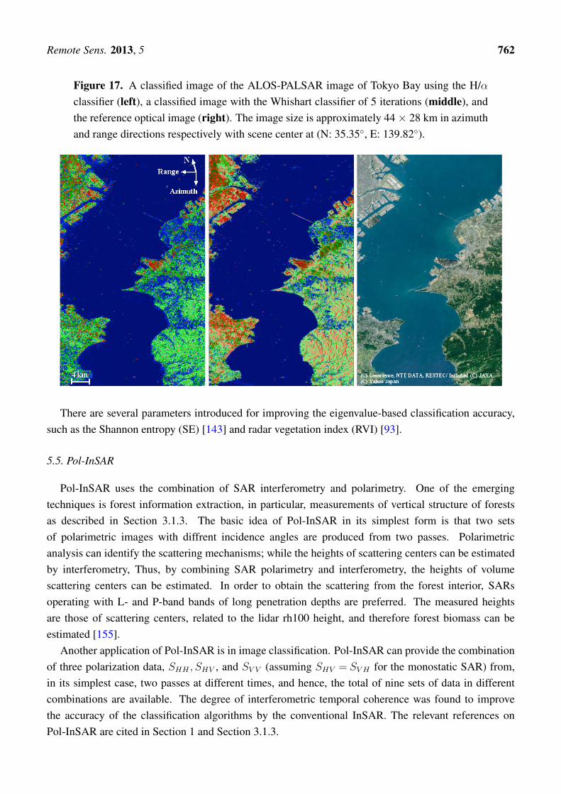
Remote Sens. 2013, 5 762
Figure 17. A classified image of the ALOS-PALSAR image of Tokyo Bay using the H/αclassifier (left), a classified image with the Whishart classifier of 5 iterations (middle), andthe reference optical image (right). The image size is approximately 44 × 28 km in azimuthand range directions respectively with scene center at (N: 35.35◦, E: 139.82◦).
There are several parameters introduced for improving the eigenvalue-based classification accuracy,such as the Shannon entropy (SE) [143] and radar vegetation index (RVI) [93].
5.5. Pol-InSAR
Pol-InSAR uses the combination of SAR interferometry and polarimetry. One of the emergingtechniques is forest information extraction, in particular, measurements of vertical structure of forestsas described in Section 3.1.3. The basic idea of Pol-InSAR in its simplest form is that two setsof polarimetric images with diffrent incidence angles are produced from two passes. Polarimetricanalysis can identify the scattering mechanisms; while the heights of scattering centers can be estimatedby interferometry, Thus, by combining SAR polarimetry and interferometry, the heights of volumescattering centers can be estimated. In order to obtain the scattering from the forest interior, SARsoperating with L- and P-band bands of long penetration depths are preferred. The measured heightsare those of scattering centers, related to the lidar rh100 height, and therefore forest biomass can beestimated [155].
Another application of Pol-InSAR is in image classification. Pol-InSAR can provide the combinationof three polarization data, SHH , SHV , and SV V (assuming SHV = SV H for the monostatic SAR) from,in its simplest case, two passes at different times, and hence, the total of nine sets of data in differentcombinations are available. The degree of interferometric temporal coherence was found to improvethe accuracy of the classification algorithms by the conventional InSAR. The relevant references onPol-InSAR are cited in Section 1 and Section 3.1.3.
Remote Sens. 2013, 5 763
The main application of PolSAR is target classification and that of Pol-InSAR is tomography.However, the measurement accuracies have not yet been fully proven in a strictly quantitative manner asthose of InSAR and DInSAR, since there are not enough reports on the comparisons using ground-truthdata, in particular, for image classification. Nevertheless, there is no doubt that quad-polarization SARdata contain much information on the scattering targets in comparison with single- and dual-polarizationdata, and radar polarimetry is expected to provide a new tool for the various fields of science andengineering in the near future.
6. Conclusions
Recent trend and advances of the state-of-the-art SAR technologies are described in this article withselected applications ranging from the conventional SAR, InSAR and DInSAR to polarimetric SAR.As is well known, increasing number of airborne SARs have been built and increasing numbers ofspaceborne SARs have been launched during the last several decades. This is due to the all-weatherand day-and-night imaging capabilities of SAR, and because the spatial resolution is improving (upto submetric) and becoming comparable with that of optical sensors. One of the interesting trends isthe increasing number of light-weight SARs. Although satellites with multiple sensors have their ownadvantages, a constellation of these compact sole-SAR satellites enables to reduce revisit intervals thathave been a major problem in satellite remote sensing. The feasibilities of bistatic SARs and digitalbeam forming are also tested using airborne SAR systems.
Amplitude is the most basic parameter in SAR data, containing information on the electric andstructural properties of scattering objects. Alongside with interferometry and polarimetry, utilizationof amplitude data in single polarization and combination of different polarizations will be continuedin various applications such as measurements of forest biomass and soil moisture, monitoring ofagricultural crops, extraction of geological features, disaster monitoring and mitigation, and those listedin Table 1. Applications of amplitude information in oceanography include the spectral estimationof ocean waves leading to improvement in wave forecast and providing real or semi-real time waveinformation, and measurements of oceanic internal waves leading to deeper understanding of theinteraction between continental shelf and deep water, their effects on phytoplankton and fishery, andthe effects on marine architecture and underwater communications. Measurements of ocean wind fieldby SAR can be made in much finer scale than wind scatterometers. Although further study is requiredfor the determination of wind direction, this application is particularly useful in estimating wind fieldnear coastal waters where the measurements are difficult to make by scatterometers of coarse resolution(order of several to few tens of kilometers). Amplitude data can also be used to monitor the spatialand temporal variations of oil slicks, major currents, fronts, and icebergs and sea ice in cryosphere.Ship detection and identification by SAR and combined with AIS are another application for combatingincreasing maritime crimes, monitoring and controlling of maritime traffics, and fishery.
Cross-track InSAR and DInSAR utilize the phase information of complex SAR images. Thistechnology is matured to an established technique for producing DEM and measurements of surfacemovement and deformation caused by earthquakes, volcanic activities, and glacier flows. Followingthe DEM of the earth by the SRTM mission in 2000, a higher resolution digital elevation model
Remote Sens. 2013, 5 764
of which the characteristics are listed in Table 5 is currently being made using TerraSAR-X andTanDEM-X data. DInSAR has been used extensively to evaluate the surface deformation associatedwith major earthquakes from the 1992 Landers earthquake in California to the recent 2011 Tohoku-Okiearthquake in the north-east Japan. Improved accuracy of the order of few millimeters per year can beachieved by PS-InSAR and related techniques for the deformation measurements over discrete persistentscatterers as well as distributed scatterers. Cross-track DInSAR measures the surface deformation onlyin the line-of-sight (slant-range) direction, but MAI (multiple aperture interferometry) can measure thealong-track (azimuth) displacement by making forward- and backward-looking interferograms frommulti-look (2-looks in general) processed sub-images before and after an event. By combining withthe conventional DInSAR technique, two-dimensional surface deformation can then be measured. Theuse of InSAR is not limited to the DEM generation and measurements of surface deformation, butcan also be applied to forestry. Although the technique and its accuracy are under study, the InSARcoherence is shown to be a useful parameter for tree height estimation. Unlike the CT-InSAR systemusing multiple antennas (for airborne systems) or multiple baselines (for both airborne and spacebornesystems) separated in the cross-track direction, the along-track InSAR system uses multiple antennasalong the platform direction, and measures current fields over oceans and rivers; it can also be used forMTI (moving target indicator). AT-InSAR has been limited to the airborne system due to the technicaldifficulty of placing multiple antennas on a satellite, but the antennas of TerraSAR-X and TanDEM-X aresplit into two sections in the along-track direction, enabling AT-InSAR from space. The current velocitymeasured by AT-InSAR is proportional to the time lag between the two antennas, so that the measurablelower velocity is limited by the small separation of the split antenna of TerraSAR-X (and TanDEM-X).However, the formation flight by these two satellites, currently being experimented, should yield flexibleand extended range of velocity measurements.
Polarimetry is a recent emerging state-of-the-art technology, and expanding the present SARtechnology to the field of new dimension. PolSAR and Pol-InSAR have been used by airborne systems,but with the launch of the first spaceborne fully polarimetric ALOS-PALSAR in 2006, interest hasaccelerated with great enthusiasm resulting in substantial numbers of research publications. In themodel-based scattering power decomposition analysis, the backscattered power can be decomposed intothree or four components of different scattering mechanisms, and thus the technique is used for a newtype of image classification, which cannot be achieved by amplitude data alone. Eigenvalue analysis candetermine the randomness of scattering by the entropy, and different scattering processes by the alphaangle. Using these two parameters in Cartesian coordinates, a new classification scheme based on thescattering process has been proposed, which can be expanded to a three-dimensional space using theanisotropy or total power. Many other classifiers based on feature vector in feature space using PolSARdata have been proposed, including one based on the Whishart distribution. While these techniques arebased on statistical averaging, pixel-based non-statistical analyses such as the Pauli decomposition havebeen used for target detection and classification. Pol-InSAR is a new technique combining polarimetryand interferometry. The former is used for classification of scattering mechanisms, and the latter forheight measurements. Thus, Pol-InSAR can be applied to estimating the height of a target having aparticular scattering process, e.g., surface, double-bounce, or volume scattering, and as such, can be usedto measure tree height. Pol-InSAR using L-band or P-band of long penetration depth can also be used for
Remote Sens. 2013, 5 765
tomography. A recent interesting new scheme is compact polarimetric SAR (CP-SAR). CP-SAR cannotprovide the full polarimetric information that can be obtained by the conventional quad-polarization data,but it has advantages of reducing the transmission power and hardware requirements, and also mitigatingthe ionospheric effects. SAR polarimetry is at a developing stage, and for practical applications, itrequires further effort for stringent validation of its methodology.
As to the present status of spaceborne SARs, CosmoSkyMed and SAR-Lupe series, andRADARSAT-2 are in operation, and TanDEM-X with TerraSAR-X has started to produce new results.Reflecting these recent trends, new spaceborne and airborne SARs are being planned by the agenciesand institutes of various countries. Using the great amount of these data, much advance is expectedin research, developing and validating new SAR technologies, and in applications to geoscience andrelated fields.
Acknowledgements
The author should like to thank the two reviewers and external editor for very constructive commentsand suggestions to improve this paper. The author is also grateful to M. Sugimoto of NationalDefense Academy, Japan for processing ALOS-PALSAR data, and to G.M. Martin of GMV Aerospace,Spain for providing information on ship detection and identification. Thanks are also due the JapanAerospace Exploration Agency (JAXA) and European Space Agency (ESA) for cordially providingALOS-PALSAR and ERS-1 SAR data respectively. Pi-SAR data were provided by the National Instituteof Information and Communications Technology (NICT), and JAXA.
References
1. Wiley, C.A. Synthetic aperture radars—A paradigm for technology evolution. IEEE Trans.Aerosp. Electron. Syst. 1985, 21, 440–443.
2. Watson-Watt, Sir, R. Three Steps to Victory; Odhams Press: London, UK, 1957.3. Jordan, R.L. The Seasat—A synthetic aperture radar system. IEEE J. Ocean. Eng. 1980, 5,
154–164.4. Evans, D.L.; Alpers, W.; Cazanave, A.; Elach, C.; Farr, T.; Glakin, D.; Holt, B.; Jones, L.;
Liu, W.T.; McCandless, W.; et al. Seasat—A 25-year legacy of success. Remote Sens. Environ.2005, 94, 384–404.
5. Curlander, J.C.; McDonough, R.N. Synthetic Aperture Radar: Systems and Signal Processing;Wiley: New York, NY, USA, 2001.
6. Elachi, C. Spaceborne Radar Remote Sensing: Applications and Technologies; IEEE Press:New York, NY, USA, 1988.
7. Ulaby, F.T.; Moore, R.K.; Fung, A.K. Microwave Remote Sensing: Active and Passive;Addison-Wesley: Reading, MA, USA, 1986; Volume I, pp. 2–3.
8. Attema, E.P.W. The active microwave instrument on-board the ERS-1 satellite. Proc. IEEE 1991,79, 791–799.
9. Cimino, J.; Elachi, C.; Settle, M. SIR-B-the second Shuttle Imaging Radar experiment. IEEETrans. Geosci. Remote Sens. 1986, GE-24, 445–452.
Remote Sens. 2013, 5 766
10. Granger, J.L. Shuttle Imaging Radar-A/B Sensors. In Proceedings of First Spaceborne ImagingRadar Symposium, Pasadena, CA, USA, 17–20 January 1983; , JPL Pub. 83-11, pp. 26–31.
11. Jordan, R.L.; Huneycutt, B.L.; Werner, M. The SIR-C/X-SAR synthetic aperture radar system.Proc. IEEE 1991, 79, 827–838.
12. Evans, D.L. Spaceborne imaging radar-C/X-band synthetic aperture radar (SIR-C/X-SAR):A look back on the tenth anniversary. IEEE Proc. Radar Son. Nav. 2006, 153, 81–85.
13. Farr, T.G.; Kobrick, M. Shuttle radar topography mission produces a wealth of data. EOS Trans.AGU 2000, 81, 583–585.
14. Werner, M. Shuttle Radar Topography Mission (SRTM), Mission overview. Frequenz 2001, 55,75–79.
15. Rabus, B.; Eineder, M.; Roth, A.; Bamler, R. The shuttle radar topography mission—A newclass of digital elevation models acquired by spaceborne radar. ISPRS J. Photogramm. 2003, 57,241–262.
16. Shimada, M. SAR programmes in JAXA: From JERS-1 to the future. IEE Proc. Radar Son.Navig. 2006, 153, 122–128.
17. Rosenqvist, A.; Shimada, M.; Ito, N.; Watanabe, M. ALOS PALSAR: A pathfinder missionfor global-scale monitoring of the environment. IEEE Trans. Geosci. Remote Sens. 2007, 45,3307–3316.
18. Shimada, M.; Tadono, T.; Rosenqvist, A. Advanced Land Observing Satellite (ALOS) andmonitoring global environmental change. Proc. IEEE 1010, 98, 780–799.
19. Nemoto, Y.; Nishino,H.; Ono, M.; Mizutamari, H.; Nishikawa, K.; Tanaka, K. Japanese EarthResources Satellite-1 synthetic aperture radar. Proc. IEEE 1991, 79, 800–809.
20. Moon, W.M.; Staples, G.; Kim, D.-J.; Park, S.-E.; Park, K.-A. RADARSAT-2 and coastalapplications: Surface wind, waterline, and intertidal flat roughness. Proc. IEEE 2010, 98,800–815.
21. Raney, R.K.; Luscombe, A.P.; Langham, E.J.; Ahmed, S. RADARSAT. Proc. IEEE 1991, 79,839–849.
22. Krieger, G.; Hajnsek, I.; Papathanassiou, P.; Younis, N.; Moriera, A. Interferometric syntheticaperture radar (SAR) missions employing formation flying. Proc. IEEE 2010, 98, 816–843.
23. COSMO-SkyMed Web Site. Available online: http://www.cosmo-skymed.it/en/index.htm(accessed on 14 November 2012).
24. Torre, A.; Capece, P. COSMO-SkyMed: The Advanced SAR Instrument. In Proceedings of 20115th International Conference on Recent Advances in Space Technologies (RASAT), Rome, Italy,9–11 June 2011; pp. 865–868.
25. Reale, D.; Nitti, D.O.; Peduto, D.; Nutricato, R.; Bovenga, F.; Fornaro, G. Postseismicdeformation monitoring with the COSMO/SKYMED constellation. IEEE Geosci. Remote Sens.Lett. 2011, 8, 696–700.
26. The RADARSAT Constellation Program. Available online: http://www.asc-csa.gc.ca/pdf/radarsat constellation eng.pdf (accessed on 14 November 2012).
Remote Sens. 2013, 5 767
27. Colinas, J.; Seguin, G.; Plourde, P. Radarsat Constellation, Moving toward Implementation.In Proceedings of IEEE International Geoscience and Remote Sensing Symposium (IGARSS),Honolulu, HI, USA, 25–30 July 2010; pp. 3232–3235.
28. Thompson, A.A. Innovative Capabilities of the RADARSAT Constellation Mission. InProceedings of 8th European Conference on Synthetic Aperture Radar (EUSAR), Aachen,Germany, 7–10 June 2010.
29. Stevens, D.R.; Cumming, I.G.; Gray, A.L. Options for airborne interferometric SAR motioncompensation. IEEE Trans. Geosci. Remote Sens. 1995, 3, 409–420.
30. Prats, P.; de Macedo, K.A.C.; Reigber, A.; Scheiber, R.; Mallorquı, J.J. Comparison oftopography-and aperture-dependent motion compensation algorithms for airborne SAR. IEEEGeosci. Remote Sens. Lett. 2007, 4, 349–353.
31. Brown, W.D.; Ghiglia, D.C. Some methods for reducing propagation-induced phase errors incoherent imaging systems. Part I. Formalism. J. Opt. Soc. Am. 1988, A5, 924–942.
32. Ghiglia, D.C.; Mastin, G.A. Two-dimensional phase correction of synthetic-aperture-radarimagery. Opt. Let. 1989, 14, 1104–1106.
33. Oliver, C.J. Synthetic-aperture radar imaging. J. Phys. D 1989, 22, 871–980.34. Werness, S.; Carrara, W.; Joyce, L.; Franczak, D. Moving target imaging algorithms for SAR
data. IEEE Trans. Aerosp. Electron. Syst. 1990, 26, 57–67.35. Yoji, G.N. Phase Difference Auto Focusing for Synthetic Aperture Radar Imaging. US Patent
No. 4,999,635, 12 March 1991.36. Eichel, P.H.; Jakpwatz, G.V., Jr. Phase-gradient algorithm as an optimal estimator of the phase
derivative. Opt. Let. 1989, 14, 1101–1103.37. Wahl, D.E.; Eichel, P.H.; Ghiglia, D.C.; Jakpwatz, G.V., Jr. Phase gradient autofocus—A robust
tool for high resolution SAR phase correction. IEEE Trans. Aerosp. Electron. Syst. 1994, 30,827–834.
38. Kolman, J. PACE: An Autofocus Algorithm for SAR. In Proceedings of 2005 IEEE InternationalRadar Conference, Arlington, VA, USA, 9–12 May 2005; pp. 310–314.
39. Yang, J.; Huang, X.; Jin, J.; Xue, G.; Zhou, Z. An interpolated phase adjustment by contrastenhancement algorithm for SAR. IEEE Geosci. Remote Sens. Lett. 2011, 8, 211–214.
40. Wang, J.; Liu, X. SAR minimum-entropy autofocus using an adaptive-order polynomial model.IEEE Geosci. Remoe Sens. Lett. 2006, 3, 512–516.
41. Samczynski, P.; Kulpa, K.S. Coherent MapDrift technique. IEEE Trans. Geosci. Remote Sens.2010, 48, 1505–1517.
42. Samczynski, P. Superconvergent velocity estimator for an autofocus coherent MapDriftTechnique. IEEE Geosci. Remote Sens. Lett. 2012, 9, 204–208.
43. Kersten, P.R.; Jansen, R.W.; Luc, K.; Ainsworth, T.L. Motion analysis in SAR images ofunfocused objects using time-frequency methods. IEEE Geosci. Remote Sens. Lett. 2007, 4,527–531.
44. Ash, J.N. An autofocus method for backprojection imagery in synthetic aperture radar. IEEEGeosci. Remote Sens. Lett. 2012, 9, 104–108.

Remote Sens. 2013, 5 768
45. Hanssen, R.F. Radar Interferometry: Data Interpretation and Error Analysis; Kluwer AcademicPublishers: Dordrecht, The Netherlands, 2001.
46. Massonnet, D.; Souyris, J.-C. SAR Interferometry: Towards the Ultimate Ranging Accuracy. InImaging with Synthetic Aperture Radar; CRC Press, Taylor Francis Group: Boca Raton, FL, USA,2008; Chapter 4, pp. 177–228.
47. Graham, L.C. Synthetic interferometer radar for topographic mapping. Proc. IEEE 1974, 62,763–768.
48. Rodriguez, E.; Martin, J.M. Theory and design of interferometric SARs. Proc. IEEE 1992, 139,147–159.
49. Gens, R.; van Genderen, J.L. SAR interferometry-Issues, techniques, applications. Int. J. RemoteSens. 1996, 17, 1803–1835.
50. Bamler, R.; Hartl, P. Synthetic aperture radar interferometry. Inverse Probl. 1998, 14, R1–R54.51. Rosen, P.; Hensley, S.; Joughin, I.R.; Li, F.K.; Madsen, S.N.; Rodriguez, E.; Goldstein, R.
Synthetic aperture radar interferometry. Proc. IEEE 2000, 88, 333–382.52. Gabriel, A.K.; Goldstein R.M.; Zebker H.A. Mapping small elevation changes over large areas:
Differential radar interferometry. J. Geophys. Res. 1989, 94, 9183–9191.53. Massonnet, D.; Feigl, K. Radar interferometry and its application to changes in the earth’s surface.
Rev. Geophys. 1998, 36, 441–500.54. Ferretti, A.; Prati, C.; Rocca, F. Nonlinear subsidence rate estimation using permanent scatterers
in differential SAR interferometry. IEEE Trans. Geosci. Remote Sens. 2000, 38, 2202–2212.55. Ferretti, A.; Prati, C.; Rocca, F. Permanent scatterers in SAR interferometry. IEEE Trans. Geosci.
Remote Sens. 2001, 39, 8–20.56. Hilley, G.E.; Bergmann, R.; Ferretti, A.; Novali, F.; Rocca, F. Dynamics of slow-moving
landslides from permanent scatter analysis. Science 2004, 304, 1952–1955.57. Van der Kooij, M.; Hughes, W.; Sato, S.; Poncos, V. Coherent Target Monitoring at High
Spatial Density: Examples of Validation Results. In Proceedings of the Advances in the Scienceand Applications of SAR Interferometry, ESA Fringe 2005, Workshop, ESA, Frascati, Italy,28 November–2 December 2005. Available online: http://earth.esa.int/fringe05/proceedings/(accessed on 15 November 2012).
58. Kampes, B.M. Radar Interferometry—Persistent Scatterer Technique; Springer: Dordrecht, TheNetherlands, 2006.
59. Rocca, F. Modeling interferogram stacks. IEEE Trans. Geosci. Remote Sens. 2007, 45,3289–3299.
60. InSAR CTM. Available online: http://www.gisat.cz/images/upload/6185b ev-ctm.pdf (accessedon 15 November 2012)
61. Blanco-Sanchez, P.; Mallorquı, J.J.; Duque, S.; Monells, D. The coherent pixels technique (CPT):An advanced DInSAR technique for nonlinear deformation monitoring. Pure Appl. Geophys.2008, 165, 1167–1194.
62. Crosetto, M.; Monserrat, O.; Cuevas, M.; Crippa, B. Spaceborne differential SAR interferometry:Data analysis tools for deformation measurement. Remote Sens. 2011, 3, 305–318.
Remote Sens. 2013, 5 769
63. Goldstein, R.M.; Zebker, H.A. Interferometric radar measurements of ocean surface currents.Nature 1987, 328, 707–709.
64. Shemer, L.; Marom M.; Markman D. Estimates of currents in the nearshore ocean region usinginterferometric synthetic aperture radar. J. Geophys. Res. 1993, 98, 7001–7010.
65. Shemer, L.; Marom M. Estimates of ocean coherence time by an interferometric SAR. Int. J.Remote Sens. 1993, 14, 3021–3029.
66. Carande, R.E. Estimating ocean coherence time using dual-baseline interferometric syntheticaperture radar. IEEE Trans. Geosci. Remote Sens. 1994, 32, 846–854.
67. Ainsworth, T.L.; Chubb, S.R.; Fusina, R.A.; Goldstein, R.M.; Jansen, R.W.; Lee, J.-S.;Valenzuela, J.S. INSAR imagery of surface currents, wave fields, and fronts. IEEE Trans. Geosci.Remote Sens. 1995, 33, 1117–1123.
68. Frasier, S.J.; Camps, A.J. Dual-beam interferometry for ocean surface current vector mapping.IEEE Trans. Geosci. Remote Sens. 2001, 39, 404–414.
69. Siegmund, R.; Bao, M.; Lehner, S.; Mayerle, R. First demonstration of surface currents imagedby hybrid along- and cross-track interferometric SAR. IEEE Trans. Geosci. Remote Sens. 2004,42, 511–519.
70. Romeiser, R.; Breit, H.; Eineder, M.; Runge, H.; Flament, P.; Karin, de Jong; Vogelzang, J.Current measurements by SAR along-track interferometry from a Space Shuttle. IEEE Trans.Geosci. Remote Sens. 2005, 43, 2315–2324.
71. Toporkov, J.V.; Perkovic, D.; Farquharson, G.; Sletten, M.A.; Frasier, S.J. Sea surface velocityvector retrieval using dual-beam interferometry: First demonstration. IEEE Trans. Geosci.Remote Sens. 2005, 43, 2494–2502.
72. Romeiser, R.; Runge, H. Current Measurements in Coastal Waters and Rivers by Along-TrackInSAR. In Remote Sensing of the European Seas; Barale, V., Gade, M., Eds.; Springer: Berlin,Germany, 2008; pp. 411–422.
73. Romeiser, R.; Suchandt, S.; Runge, H.; Steinbrecher, U.; Grunler, S. First analysis of TerraSAR-Xalong-track InSAR-derived current fields. IEEE Trans. Geosci. Remote Sens. 2010, 48, 820–829.
74. Breit, H.; Eineder, M.; Holzner, J.; Runge, H.; Bamler, H. Traffic Monitoring Using SRTMAlong-Track Interferometry. In Proceedings of IEEE International Geoscience and RemoteSensing Symposium (IGARSS), Toulouse, France, 21–25 July 2003; Volume II, pp. 1187–1189.
75. Lombardo, P.; Colone, F.; Pastina, D. Monitoring and surveillance potentialities obtained bysplitting the antenna of the COSMO-SkyMed SAR into multiple sub-apertures. IEE Proc. RadarSon. Navig. 2006, 153, 104–116.
76. Meyer, F.; Hinz, S.; Laika, A.; Weihing, D.; Bamler, R. Performance analysis of the TerraSAR-Xtraffic monitoring concept. ISPRS J. Photogramm. 2006, 61, 225–242.
77. Kohlleppel, R.; Gierull, C.H. Enhancement of Along-Track Interferometry for Ground MovingTarget Indication. In Proceedings of IEEE International Geoscience and Remote SensingSymposium (IGARSS), Boston, MA, USA, 7–11 July 2008; Volume II, pp. 229–232.
78. Yang, L.; Wang, T.; Bao, Z. Ground moving target indication using an InSAR system with ahybrid baseline. IEEE Geosci. Remote Sens. Lett. 2008, 5, 373–377.
Remote Sens. 2013, 5 770
79. Suchandt, S.; Runge, H.; Breit, H.; Steinbrecher, U.; Kotenkov, A.; Balss, U. Automatic extractionof traffic flows using TerraSAR-X along-track interferometry. IEEE Trans. Geosci. Remote Sens.2010, 48, 807–819.
80. Van Zyl, J.J. Imaging radar polarization signatures: Theory and observation. Radio Sci. 1987, 22,529–543.
81. Ulaby, F.T.; Elachi, C. Radar Polarimetry for Geoscience Applications; Artech House: Norwood,MA, USA, 1990.
82. Zebker, H.A.; van Zyl, J.J. Imaging radar polarimetry: A review. Proc. IEEE 1991, 79,1583–1605.
83. Mott, H. Remote Sensing with Polarimetric Radar; Wiley: New York, NY, USA, 2007.84. Massonnet, D.; Souyris, J.-C. SAR Polarimetry: Towards the Ultimate Characterization of
Targets. In Imaging with Synthetic Aperture Radar; CRC Press, Taylor & Francis Group: BocaRaton, FL, USA, 2008; Chapter 5, pp. 229–272.
85. Lee, J.-S.; Pottier, E. Polarimetric Radar Imaging—From Basics to Applications; CRC Press,Taylor & Francis Group: Boca Raton, FL, USA, 2009.
86. Cloude, S.R. Polarisation: Application in Remote Sensing; Oxford University Press: Oxford,UK, 2009.
87. Van Zyl, J.J.; Kim, Y.J. Synthetic Aperture Radar Polarimetry; Wiley: New York, NY, USA, 2011.88. Kostinski, A.B.; James, B.D.; Boerner, W.-M. Polarimetric matched filter for coherent imaging.
Can. J. Phys. 1988, 66, 817–877.89. Swarts, A.A.; Yueh, H.A.; Kong, J.A.; Novak, L.M.; Shin, R.T. Optimal polarization for achieving
maximum contrast in radar images. J. Geophys. Res. 1988, 93, 15252–15260.90. Boerner, W.-M.; Yan, W.L.; Xi, A.-Q.; Yamaguchi, Y. On the basic principles of radar
polarimetry: The target characteristic polarization state theory of Kennauugh, Huynen’spolarization fork concept, and its extension to the partially polarized case. Proc. IEEE 1991,79, 1538–1550.
91. Boerner, W.-M.; Walther, M.; Segal, A.C. The concept of the polarimetric matched signal &image filters: Application to radar target versus speckle reduction & optimal background clutterdiscrimination in microwave sensing and imaging. EARSeL Adv. Remote Sen. 1993, 2, 219–252.
92. Rignot, E.; Chellappa, R.; Dubois, P. Unsupervised segmentation of polarimetric SAR data usingthe covariance matrix. IEEE Trans. Geosci. Remote Sens. 1992, 30, 697–705.
93. Van Zyl, J.J. Application of Cloude’s target decomposition theorem to polarimetric imaging radar.Proc. SPIE 1993, 184, 184–191.
94. Yamaguchi, Y.; Takayanagi, Y.; Boerner, W.-M.; Eom, H.J.; Sengoku, M. Polarimetricenhancement in radar channel imagery. IEICE Trans. Commun. 1995, E78, 1571–1579.
95. Cloude, S.R.; Pottier, E. A review of target decomposition theorems in radar polarimetry. IEEETrans. Geosci. Remote Sens. 1996, 34, 498–518.
Remote Sens. 2013, 5 771
96. Cloude, S.R.; Pottier, E. An entropy based classification scheme for land applications ofpolarimetric SAR. IEEE Trans. Geosci. Remote Sens. 1997, 35, 68–78.
97. Boerner, W.-M.; Mott, H.; Lunenburg, E.; Livingstone, C.; Brisco, B.; Brown, R.J.; Patterson, J.S.Polarimetry in Remote Sensing: Basic and Applied Concepts. In Manual of Remote Sensing,Volume 2: Principles and Applications of Imaging Radar, 3rd ed.; Wiley: New York, NY, USA,1998; Chapter 5, pp. 271–358.
98. Freeman, A.; Durden, S.L. A three-component scattering model for polarimetric SAR data. IEEETrans. Geosci. Remote Sens. 1998, 36, 963–973.
99. Lee, J.-S.; Grunes, M.R.; Anisoworth, T.L.; Du, L.J.; Schuler, D.L.; Coulde, S.R. Unsupervisedclassification using polarimetric decomposition and the complex Whishart classifier. IEEE Trans.Geosci. Remote Sens. 1999, 35, 2249–2258.
100. Yang, J.; Yamaguchi, Y.; Yamada, H.; Sengoku, M.; Lin, S.-M. The optimal problem forcontrast enhancement in polarimetric radar remote sensing. IEICE Trans. Commun. 1999, E82-B,174–183.
101. Ferro-Famil, L.; Pottier, E.; Lee, J.-S. Unsupervised classification of multifrequency and fullypolarimetric SAR images based on H/A/Alpha-Whishart classifier. IEEE Trans. Geiosci. RemoteSens. 2001, 39, 2332–2342.
102. Pottier, E.; Lee, J.-S.; Ferro-Famil, L. Advanced Concepts in Polarimetry—Part 1 (PolarimetricTarget Description, Speckle Filtering and Decomposition Theorems); RTO-EN-SET-081; NATOScience and Technology Organization: Paris, France, 2004.
103. Lumsdon, P.; Cloude, S.R.; Wright, G. Polarimetric classification of land cover for Glen Affricradar project. IEEE Proc. Radar Son. Navig. 2005, 152, 404–412.
104. Yamaguchi, Y.; Moriyama, T.; Ishido, M.; Yamada, H. Four-component scattering model forpolarimetric SAR image decomposition. IEEE Trans. Geosci. Remote Sens. 2005, 43,1699–1706.
105. Xu, F.; Jin, Y.-Q. Deorientation theory of polarimetric scattering targets and application to terrainsurface classification. IEEE Trans. Geosci. Remote Sens. 2005, 43, 2351–2364.
106. Cameron, W.L.; Rais, H. Conservative polarimetric scatterers and their role in incorrect extensionsof the Cameron decomposition. IEEE Trans. Geosci. Remote Sens. 2006, 44, 3506–3516.
107. Lee, J.-S.; Krogager, E.; Ainsworth, T. L.; Boerner, W.-M. Polarimetric analysis of radar signatureof a manmade structure. IEEE Geosci. Remote Sens. Lett. 2006, 3, 555–559.
108. Touzi, R. Target scattering decomposition in terms of roll-invariant target parameters. IEEE Trans.Geosci. Remote Sens. 2007, 45, 73–84.
109. Yajima, Y.; Yamaguchi, Y.; Sato, R.; Yamada, H.; Boerner, W.-M. POLSAR image analysis ofwetlands using a modified four-component scattering power decomposition. IEEE Trans. Geosci.Remote Sens. 2008, 46, 1667–1673.
110. Zhang, L.; Zou, B.; Cai, H.; Zhang, Y. Multiple-component scattering model for polarimetricSAR image decomposition. IEEE Geosci. Remote Sens. Lett. 2008, 5, 603–607.
111. McNairn, H.; Shang, J.L.; Jiao, S.F.; Champagne, C. The contribution of ALOS PALSARmultipolarization and polarimetric data to crop classification. IEEE Trans. Geosci. Remote Sens.2009, 47, 3981–3992.
Remote Sens. 2013, 5 772
112. Praks, J.; Koeniguer, E.C.; Hallikainen, M.T. Alternatives to target entropy and alpha angle inSAR polarimetry. IEEE Trans. Geosci. Remote Sens. 2009, 47, 2262– 2274.
113. Touzi,R.; Deschamps, A.; Rother, G. Phase of target scattering for wetland characterization usingpolarimetric C-band SAR. IEEE Trans. Geosci. Remote Sens. 2009, 47, 3241–3261.
114. Li, P.; Deng, S.; Zhang, J.; Huang, G.; Zhao, Z. A Framework of Polarimetric SAR Filter Basedon Independence of Intensity and Polarimetric Information. In Proceedings of ISPRS TC VIISymposium—100 Years ISPRS, Vienna, Austria, 5–7 July 2010; Volume XXXVIII, Part 7A,pp. 117–121.
115. Marino, A.; Cloude, S.R.; Woodhouse, I.H. A polarimetric target detector using the Huynen fork.IEEE Trans. Geosci. Remote Sens. 2010, 48, 2357–2366.
116. Antropov, O.; Rauste, Y.; Hame, T. Volume scattering modeling in PolSAR decompositions:Study of ALOS PALSAR data over boreal forest. IEEE Trans. Geosci. Remote Sens. 2011,49, 3838–3848.
117. Arii, M.; van Zyl, J.J.; Kim, Y. Adaptive model-based decomposition of polarimetric SARcovariance matrices. IEEE Trans. Geosci. Remote Sens. 2011, 49, 1104–1113.
118. Yamaguchi, Y.; Sato, A.; Boerner, W. M.; Sato, R.; Yamada, H. Four-component scattering powerdecomposition with rotation of coherency matrix. IEEE Trans. Geosci. Remote Sens. 2011, 49,2251–2258.
119. Van Zyl, J.J.; Arii, M.; Kim, Y. Model-based decomposition of polarimetric SAR covariancematrices constrained for nonnegative eigenvalues. IEEE Trans. Geosci. Remote Sens. 2011, 49,3452–3459.
120. Li, K.; Brisco, B.; Yun, S.; Touzi, R. Polarimetric decomposition with RADARSAT-2 for ricemapping and monitoring. Can. J. Remote Sens. 2012, 38, 169–179.
121. Pajares, G.; Lopez-Martinez, C.; Sanchez-Llado, F.J.; Molina, I. Improving Wishart classificationof polarimetric SAR data using the Hopfield Neural Network optimization approach. RemoteSens. 2012, 4, 3571–3595.
122. Ramsey, E., III; Rangoonwala, A.; Suzuoki, Y.; Jones, C.E. Oil detection in a coastal marsh withpolarimetric synthetic aperture radar (SAR). Remote Sens. 2011, 3, 2630–2662.
123. Sato, A.; Yamaguchi, Y.; Singh, G.; Park, S.-E. Four-component scattering power decompositionwith extended volume scattering model. IEEE Geosci. Remote Sens. Lett. 2012, 9, 166–170.
124. Shan, Z.; Wang, C.; Zhang, H.; An, W. Improved four-component model-based targetdecomposition for polarimetric SAR data. IEEE Geosci. Remote Sens. Lett. 2012, 9, 75–79.
125. Sugimoto, M.; Ouchi, K.; Nakamura, Y. Four-component scattering power decompositionalgorithm with rotation of covariance matrix using ALOS-PALSAR polarimetric data. RemoteSens. 2012, 4, 2199–2209.
126. Watanabe, M.; Yonezawa, C.; Iisaka, J.; Sato, M. ALOS/PALSAR full polarimetric observationsof the Iwate-Miyagi Nairiku earthquake of 2008. Int. J. Remote Sens. 2012, 33, 1234–1245.
127. Yonezawa, C.; Watanabe, M.; Saito, G. Polarimetric decomposition analysis of ALOS-PALSARobservation data before and after a landslide event. Remote Sens. 2012, 4, 2314–2328.
128. Wright, P.A.; Quegan, S.; Wheadon, N.S.; Hall, C.D. Faraday rotation effects on L-bandspaceborne SAR data. IEEE Trans. Geosci. Remote Sens. 2003, 41, 2735–2744.

Remote Sens. 2013, 5 773
129. Jehle, M.; Ruegg, M.; Small,D.; Meier, E.; Nuesch, D. Estimation of ionospheric TEC andFaraday rotation for L-band SAR. Proc. SPIE 2005, doi: 10.1117/12.627618.
130. Qi, R.-Y.; Jin, Y.-Q. Analysis of the effects of Faraday rotation on spaceborne polarimetric SARobservations at P-band. IEEE Trans. Geosci. Remote Sens. 2007, 45, 1115–1122.
131. Meyer, F.J.; Nicoll, J.B. Prediction, detection, and correction of Faraday rotation infull-polarimetric L-band SAR data. IEEE Trans. Geosci. Remote Sens. 2008, 46, 3076–3086.
132. Jehle, M.; Ruegg, M.; Zuberbuhler, L.; Small, D.; Meier, E. Measurement of ionospheric Faradayrotation in simulated and real spaceborne SAR data. IEEE Trans. Geosci. Remote Sens. 2009,47, 1512–1523.
133. Kimura, H. Calibration of polarimetric PALSAR imagery affected by Faraday rotation usingpolarization orientation. IEEE Trans. Geosci. Remote Sens. 2009, 47, 3943–3950.
134. Takeshiro, A.; Furuya, T.; Fukuchi, H. Verification of polarimetric calibration method includingFaraday rotation compensation using PALSAR data. IEEE Trans. Geosci. Remote Sens. 2009,47, 3960–3968.
135. Truong-Loi, M.-L.; Freeman, A.; Dubois-Fernandez, P.C.; Pottier, E. Estimation of soil moistureand Faraday rotation from bare surfaces using compact polarimetry. IEEE Trans. Geosci. RemoteSens. 2009, 47, 3608–3615.
136. Cloude, S.R.; Papathanassiou, K.P. Polarimetric SAR interferometry. IEEE Trans. Geosci.Remote Sens. 1998, 36, 1551–1563.
137. Reigber, A.; Moriera, A. First demonstration of airborne SAR tomography using multibaselineL-band data. IEEE Trans. Geosci. Remote Sens. 2000, 38, 2142–2152.
138. Treuhaft, R.N.; Siqueira, P.R. Vertical structure of vegetated land surfaces from interferometricand polarimetric radar. Radio Sci. 2000, 53, 141–177.
139. Papathanassiou, K.P.; Cloude, S.R. Single-baseline polarimetric SAR interferometry. IEEE Trans.Geosci. Remote Sens. 2001, 39, 2352–2363.
140. Cloude, S.R.; Papathanassiou, K.P. Three-stage inversion process for polarimetric SARinterferometry. IEEE Proc. Radar Son. Navig. 2003, 150, 125–134.
141. Aulinger, T.; Mette, T.; Papathanassiou, K.P.; Hajnsek, I.; Heurich, M.; Krzystek, P.Validation of Heights from Interferometric SAR and Lidar over the Temperate Forest Site“National Park Bayerischer Wald”. In Proceedings of the 2nd International Workshop POLINSAR2005 (ESA SP-586), ESRIN, Frascati, Italy, 17–21 January 2005.
142. Boerner, W.-M. Applications of Polarimetric and Interferometric SAR to Environmental RemoteSensing and Its Activities: Recent Advances in Extrawideband Polarimetry, Interferometry andPolarimetric Interferometry in Synthetic Aperture Remote Sensing and Its Applications. Availableonline: http://www.cso.nato.int/ (accessed on 15 November 2012).
143. Morio, J.: Refregier, P.; Goudail, F.; Dubois-Fernandez, P.; Dupuis, X. Application of InformationTheory Measures to Polarimetric and Interferometric SAR Images. In Proceedings of 5thInternational Conference on Physics in Signal & Image Processing (PSIP), Mulhouse, France,30 January–2 February 2007.
Remote Sens. 2013, 5 774
144. Praks, J.; Kugler, F.; Papathanassiou, K.P.; Hajnsek, I.; Hallikainen, M. Tree height estimationfor boreal forest by means of L- and X- band POLInSAR and HUTSCAT profiling scatterometer.IEEE Geosci. Remote Sens. Lett. 2007, 4, 466–470.
145. Lambardini, F.; Pardini, M. 3-D SAR tomography: The multibaseline sector interpolationapproach. IEEE Geosci. Remote Sens. Lett. 2008, 5, 630–634.
146. Garestier, F.; Dubois-Fernandez, P.C.; Papathanassiou, K.P. Pine forest height inversion usingsingle-pass X Band PolInSAR data. IEEE Trans. Geosci. Remote Sens. 2008, 46, 59–68.
147. Hajnsek, I.; Kugler, F.; Lee, S.-K.; Papathanassiou, K.P. Tropical-forest-parameter estimation bymeans of Pol-InSAR: The INDREX-II campaign. IEEE Trans. Geosci. Remote Sens. 2009, 47,481–493.
148. Tebaldini, S. Algebraic synthesis of forest scenarios from multibaseline PolInSAR data. IEEETrans. Geosci. Remote Sens. 2009, 47, 4132–4142.
149. Gama, F.F.; Santos, J.R.D.; Mura, J.C. Eucalyptus biomass and volume estimation usinginterferometric and polarimetric SAR data. Remote Sens. 2010, 2, 939–956.
150. Neumann, M.; Ferro-Famil, L.; Reigber, A. Estimation of forest structure, ground, and canopylayer characteristics from multibaseline polarimetric interferometric SAR data. IEEE Trans.Geosci. Remote Sens. 2010, 48, 1086–1104.
151. Tebaldini, S. Single and multipolarimetric SAR tomography of forested areas: A parametricapproach. IEEE Trans. Geosci. Remote Sens. 2010, 48, 2375–2387.
152. Tabaldini, S.; Guarieri, A.M. On the role of phase stability in SAR multibaseline applications.IEEE Trans. Geosci. Remote Sens. 2010, 48, 2953–2966.
153. d’Alessandro, M.M.; Tebaldini, S. Phenomenology of P-band scattering from a tropical forestthrough three-dimensional SAR tomography. IEEE Geosci. Remote Sens. Lett. 2012, 9, 442–446.
154. Kobayashi, S.; Omura, Y.; Sanga-Ngoie, K.; Widyorini, R.; Kawai, S.; Supriadi, B.;Yamaguchi, Y. Characteristics of decomposition powers of L-band multi-polarimetric SAR inassessing tree growth of industrial plantation forests in the tropics. Remote Sens. 2012, 4,3058–3077.
155. Neumann, M.; Saatchi, S.S.; Ulander, L.M.H.; Fransson, R.E.S. Assessing performance of L- andP-band polarimetric interferometric SAR data in estimating boreal forest above-ground biomass.IEEE Trans. Geosci. Remote Sens. 2012, 50, 714–726.
156. Tebaldini, S.; Rocca, F. Multibaseline polarimetric SAR tomography of a boreal forest at P- andL-bands. 2012, 50, 232–246.
157. Keydel, W. Present and Future Airborne and Space-Borne Systems. Available online:http://www.dtic.mil/cgi-bin/GetTRDoc?AD=ADA470890 (accessed on 22 January 2013).
158. Krieger, G.; Hajnsek, I.; Papathanassiou, K.; Eineder, M.; Younis, M.; De Zan, F.;Lopez-Dekker, P.; Huber, S.; Werner, M.; Prats, P.; et al. Tandem-L: A Mission for MonitoringEarth System Dynamics with High Resolution SAR Interferometry. In Proceedings of 8thEuropean Conference on Synthetic Aperture Radar (EUSAR), Aachen, Germany, 7–10 June 2010;pp. 506–509.
159. Corcoran, K.M. Higher Eyes in the Sky-The Feasibility of Moving AWACS and JSTARS Functionsinto Space; Air University Press: Montgomery, AL, USA, 1999.
Remote Sens. 2013, 5 775
160. Cherniakov, M., Ed. Bistatic Radar: Emerging Technology; John Wiley & Sons: Chechester,UK, 2007.
161. Cherniakov, M. Bistatic Radar: Theory and Practice; John Wiley & Sons: Chechester, UK, 2007.162. Nies, H.; Loffeld, O.; Natroshvili, K. Analysis and focusing bistatic airborne SAR data. IEEE
Trans. Geosci. Remote Sens. 2007, 45, 3342–3349.163. Bamler, R.; Meyer, F.; Liebhart, W. Processing bistatic SAR data from quasi-stationary
configuration. IEEE Trans. Geosci. Remote Sens. 2007, 45, 3350–3358.164. Antoniou, M.; Saini, R.; Cherniakov, M. Results of a space-surface bistatic SAR imaging
formation algorithm. IEEE Trans. Geosci. Remote Sens. 2007, 45, 3359–3371.165. Arnold-Bos, A.; Khenchaf, A.; Martin, A. Bistatic radar imaging of the marine
environment—Part I: Theoretical background. IEEE Trans. Geosci. Remote Sens. 2007, 45,3372–3383.
166. Arnold-Bos, A.; Khenchaf, A.; Martin, A. Bistatic radar imaging of the marineenvironment—Part II: Simulation and results analysis. IEEE Trans. Geosci. Remote Sens. 2007,45, 3384–3396.
167. Goh, A.S.; Preiss, M.; Stacy, N.J.S.; Gray, S.A. Bistatic SAR experiment with the Ingara imagingradar. IET Radar Sonar Navig. 2010, 4, 426–437.
168. Rodriguez-Cassola, M.; Baumgartner, S.V.; Krieger, G.; Moreira, A. Bistatic TerraSAR-X/F-SARspaceborne-airborne SAR experiment: Description, data processing, and results. IEEE Trans.Geosci. Remote Sens. 2010, 48, 781–794.
169. Walterscheid, I.; Espeter, T.; Brenner, A.R.; Klare, J.; Ender, J.H.G.; Nies, H.; Wang, R.;Loffeld, O. Bistatic SAR experiments with PAMIR and TerraSAR-X-Setup, processing, andimage results. IEEE Trans. Geosci. Remote Sens. 2010, 48, 3268–3279.
170. Rodriguez-Cassola, M.; Prats, P.; Schulze, D.; Tous-Ramon, N.; Steinbrecher, U.; Marotti, L.;Nannini, M.; Younis, M.; Lopez-Dekker, P.; Zink, M.; et al. First bistatic spaceborne SARexperiments with TanDEM-X. IEEE Geosci. Remote Sens. Lett. 2012, 9, 33–37.
171. Krieger, G.; Moreira, A.; Fielder, H.; Hajnsek, I.; Werner, M.; Younis, M.; Zink, M. TenDEM-X:A satellite formation for high-resolution SAR interferometry. IEEE Trans. Geosci. Remote Sens.2007, 45, 3317–3341.
172. Souyris, J.-C.; Imbo, P.; Fjortoft, R.; Mingot, S.; Lee, J.-S. Compact polarimetry based onsymmetry properties of geophysical media: The π/4 mode. IEEE Trans. Geosci. Remote Sens.2005, 43, 634–646.
173. Raney, R.K. Hybrid-polarity SAR architecture. IEEE Trans. Geosci. Remote Sens. 2007, 45,3397–3404.
174. Dubois-Fernandez, P.; Souyris, J.-C.; Angelliaume, S.; Garestier, F. The compact polarimetryalternative for spaceborne SAR at low frequency. IEEE Trans. Geosci. Remote Sens. 2008, 46,3208–3222.
175. Nord, M.; Ainsworth, T.L.; Lee, J.-S.; Stacy, N. Comparison of compact polarimetric syntheticaperture radar modes. IEEE Trans. Geosci. Remote Sens. 2009, 47, 174–188.
176. Ainsworth, T.L.; Kelly, J.P.; Lee, J.-S. Classification comparisons between dual-pol, compactpolarimetric and quad-pol SAR imagery. ISPRS J. Photogramm. 2009, 64, 464–471.

Remote Sens. 2013, 5 776
177. Charbonneau, F.J.; Brisco, B.; Raney, R.K.; McNairn, H.; Liu, C.; Vachon, P.; Shang, J.;DeAbreu, R.; Champagne, C.; Merzouki, A.; et al. Compact polarimetry overview andapplications assessment. Can. J. Remote Sens. 2010, 36, S298–S315.
178. Cloude, S.R.; Goodenough, D.G.; Chen, H. Compat decomposition theory. IEEE Geosci. RemoteSens. Lett. 2012, 9, 28–32.
179. Tsunoda, S.I.; Pace, P.; Stence, J.; Woodring, M.; Hensley, W.H.; Doerry, A.W.; Walker, B.C.Lynx: A high-resolution synthetic aperture radar. Proc. SPIE 1999, 3704, 20–27.
180. Tsunoda, S.I.; Pace, P.; Stence, J.; Woodring, M.; Hensley, W.H.; Doerry, A.W.; Walker, B.C.Lynx: A High-Resolution Synthetic Aperture Radar. In Proceedings of 2000 IEEE AerospaceConference, Big Sky, MT, USA, 18–25 March 2000; Volume 5, pp. 51–58.
181. Doerry, A.W.; Dubbert, D.E.; Thompson, M.E.; Gutierrez, V.D. A portfolio of fine resolutionKa-band SAR images: Part I. Proc. SPIE 2005, 5788, 13–24.
182. Doerry, A.W.; Dubbert, D.E.; Thompson, M.E.; Gutierrez, V.D. A portfolio of fine resolutionKa-band SAR images: Part II. Proc. SPIE 2005, 5788, 185–196.
183. Patterson, M.C.L.; Brescia, A. Integrated Sensor Systems for UAS. In Proceedings of the 23rdBristol UAV System Conference, Bristol, UK, 7–9 April 2008.
184. Wang, W.-Q.; Peng, Q.; Cai, J. Waveform-diversity-based millimeter-wave UAV SAR remotesensing. IEEE Trans. Geosci. Remote Sens. 2009, 47, 691–700.
185. Madsen, S.N.; Hensley, S.; Wheeler, K.; Sadowy, G.A.; Miller, T.; Muellerschoen, R.; Lou, Y.;Rosen, P.A. UAV-based L-band SAR with precision flight path control. Proc. SPIE 2005, 5659,51–60.
186. Rosen, P.A.; Hensley, S.; Wheeler, K.; Sadowy, G.A.; Miller, T.; Shaffer, S.; Muellerschoen,R.; Jones, C.; Zebker, H.; Madsen, S.N. UAVSAR: A New NASA Airborne SAR System forScience and Technology Research. In Proceedings of IEEE Radar Conference, Verona, NY,USA, 24–27 April 2006. Available online: http://uavsar.jpl.nasa.gov/index.html (accessed on 14November 2012).
187. Kuhnert, C.; Wiesbeck, W. Overview Beamforming Principle. In Proceedings of 6th EuropeanConference on Synthetic Aperture Radar (EUSAR), Dresden, Germany, 16–18 May 2006.
188. Barton, P. Digital beam forming for radar. IEE Proc. F. Commun. Radar Signal Process. 1980,127, 266–277.
189. Curtis, T.E. Digital beam forming for sonar systems. IEE Proc. F. Commun. Radar SignalProcess. 1980, 127, 257–265.
190. Steyskal, H. Digital beam forming antenna, an introduction. Microwave J. 1987, 30, 107–124.191. Chiba, I.; Miura, R.; Tanaka, T.; Karasawa, T. Digital beam beam forming (DGF) antenna for
mobile communications. IEEE Aerosp. Electron. Syst. Magazine 1997, 12, 31–41.192. Jean, B.R.; Rouse, J.W., Jr. A multiple beam synthetic aperture radar design concept for
geoscience applications. IEEE Trans. Geosci. Remote Sens. 1983, GE-21, 201–207.193. Currie, A.; Brown, M.A. Wide-swath SAR. IEE Proc. F. Commun. Radar Signal Process. 1992,
139, 122–135.194. Callaghan, G.D.; Longstaff, I.D. Wide-swath space-borne SAR using a quad-element array. IEE
Proc. Radar Son. Navig. 1999, 146, 159–165.

Remote Sens. 2013, 5 777
195. Buckreuss, S.; Balzer, W.; Muhlbauer, P.; Werninghaus, R.; Pitz, W. The TerraSAR-X SatelliteProject. In Proceedings of IEEE International Geoscience and Remote Sensing Symposium(IGARSS), Toulouse, France, 21–25 July 2003; pp. 3096–3098.
196. Herrmann, J. TerraSAR-X Mission: The New Generation in High Resolution Satellites. InProcedings of the Anais XIII Simposio Brasilerio de Sensoriamento Remote, Florianopolis,Brazil, 21–26 April 2007; pp. 7063–7070. Available online: http://marte.dpi.inpe.br/col/dpi.inpe.br/sbsr80/2006/11.10.14.00/doc/7063-7070.pdf (accessed on 27 November 2012).
197. Younis, M.; Fischer, C.; Wiesbeck, W. Digital beamforming in SAR systems. IEEE Trans. Geosci.Remote Sens. 2003, 41, 1735–1739.
198. Krieger, G.; Gebert, N.; Moreira, A. Multidimensional waveform encoding: A new digitalbeamforming technique for synthetic aperture radar remote sensing. IEEE Trans. Geosci. RemoteSens. 2008, 46, 31–46.
199. Krieger, G.; Younis, M.; Gebert, N.; Huber, S.; Bordoni, F.; Patyuchenko, A.; Moreira, A.Advanced Digital Beamforming Concepts for Future SAR Systems. In Proceedings of IEEEInternational Geoscience and Remote Sensing Symposium (IGARSS), Honolulu, HI, USA, 25–30July 2010; pp. 245–248.
200. Freeman, A.; Krieger, G.; Rosen, P.; Younis, M.; Johnson, W.; Huber, S.; Jordan, R.; Moreira, A.SweepSAR: Beam-forming on Receive Using a Reflector-Phased Array Feed Combinationfor Spaceborne SAR. In Proceedings of IEEE Radar Conference, Pasadena, CA, USA, 4–8May 2009.
201. Younis, M.; Huber, S.; Patyuchenko, A.; Bordoni, F.; Krieger, G. Performance comparison ofreflector- and planner-antenna based digital beam-forming SAR. Int. J. Antenn. Propagat. 2009,doi:10.1155/2009/614931.
202. Gebert, N.; Krieger, G.; Moreira, A. Digital beamforming on receive: Techniques andoptimization strategies for high-resolution wide-swath SAR imaging. IEEE Trans. Aerosp.Electron. 2009, 45, 564–592.
203. Villano, M.; Krieger, G.; Moreira, A. Staggered-SAR: A New Concept for High-ResolutionWide-Swath Imaging. In Proceedings of 2012 IEEE GOLD Remote Sensing Conference, Rome,Italy, 4–5 June 2012. Available online: http://elib.dlr.de/75767/ (accessed on 15 November 2012).
204. Rincon, R.F.; Vega, M.A.; Buenfil, M.; Geist, A.; Hilliard, L.; Racette, P. NASA’s L-band digitalbeamforming synthetic aperture radar. IEEE Trans. Geosci. Remote Sens. 2011, 49, 3622–3628.
205. Fatoyinbo, T.; Ricon, R.F.; Sun, G.; Ranson, K.J. ECOSAR: A P-band Beamforming PolarimetricInterferometric SAR Instrument to Measure Ecosystem Structure and Biomass. In Proceedings ofIEEE International Geoscience and Remote Sensing Symposium (IGARSS), Vancouver, Canada,24–29 July 2011; pp. 1524–1527.
206. Rincon, R.F.; Fatoyinbo, T.; Sun, G.; Ranson, K.J.; Perrine, M.; Deshapnde, M.; Bonds, Q. TheECOSAR P-band Synthetic Aperture Radar. In Proceedings of IEEE International Geoscienceand Remote Sensing Symposium. (IGARSS), Vancouver, BC, Canada, 24–29 July 2011;pp. 1512–1515.
207. Shimada, M. Ortho-rectification and slope correction of SAR data using DEM and its accuracyevaluation. IEEE J. Sel. Top. Appl. Earth Obs. Remote Sens. 2010, 3, 657–671.
Remote Sens. 2013, 5 778
208. Angelsen, A.; Boucher, D.; Brown, S.; Merckx, V.; Streck, C.; Zarin, D. Guidelines for REDD+Reference Levels: Principles and Recommendations; Meridian Institute: Washington, DC, USA,2011. Available online: http://www.REDD-OAR.org (accessed on 15 November 2012).
209. UN-REDD Programme. Available online: http://www.un-redd.org/ (accessed on 15November 2012).
210. Attema, E.P.W.; Ulaby, F.T. Vegetation modeled as a water cloud. Radio Sci. 1978, 13, 357–364.211. Ulaby, F.T.; Sarabandi, K.; McDonald, K.; Whitt, M.; Dobson, M.C. Michigan microwave canopy
scattering model. Int. J. Remote Sens. 1990, 11, 1223–1253.212. Imhoff, M.L. A theoretical analysis of the effect of forest structure on synthetic aperture radar
backscatter and the remote sensing of biomass. IEEE Trans. Geosci. Remote Sens. 1995, 33,341–352.
213. Saatchi, S.S.; McDonald, K.C. Coherent effects in microwave backscattering models for forestcanopies. IEEE Trans. Geosci. Remote Sens. 1997, 35, 1032–1044.
214. Dobson, M.C.; Ulaby, F.T.; Le Toan, T.; Beaudoin, A.; Kasischke, E.S.; Christensen, N.Dependence of radar backscatter on coniferous forest biomass. IEEE Trans. Geosci. RemoteSens. 1992, 30, 412–415.
215. Le Toan, T.; Beaudoin, A.; Riom, J.; Guyon, D. Relating forest biomass to SAR data. IEEE Trans.Geosci. Remote Sens. 1992, 30, 402–411.
216. Ranson, K.J.; Sun, Q. Mapping biomass of a northern forest using multifrequency SAR data.IEEE Trans. Geosci. Remote Sens. 1994, 32, 388–396.
217. Beaudoin, A.; Le Toan, T.; Goze, S.; Nezry, E.; Lopes, A.; Mougin, E.; Hsu, C.C.; Han, H.C.;Long, J.A.; Shin, R.T. Retrieval of forest biomass from SAR data. Int. J. Remote Sens. 1994, 15,2777–2796.
218. Rauste, Y.; Hame, T.; Pulliainen, J.; Heiska, K.; Hallikainen, M. Radar-based forest biomassestimation. Int. J. Remote Sens. 1994, 15, 2797–2808.
219. Imhoff, M.L. Radar backscatter and biomass saturation: Ramifications for global biomassinventory. IEEE Trans. Geosci. Remote Sens. 1995, 33, 511–518.
220. Rignot, E.J.; Zimmermann, R.; van Zyl, J.J. Spaceborne applications of P band imaging radarsfor measuring forest biomass. IEEE Trans. Geosci. Remote Sens. 1995, 33, 1162–1169.
221. Watanabe, M.; Shimada, M.; Rosenqvist, A.; Tadono, T.; Matsuoka, M.; Romshoo, S.A.;Ohta, K.; Furuta, R.; Nakamura, K.; Moriyama, T. Forest structure dependency of the relationbetween L-band σ0 and biophysical parameters. IEEE Trans. Geosci. Remote Sens. 2006, 44,3154–3165.
222. Mohan, S.; Das, A.; Halder, D.; Maity, S. Monitoring and Retrieval of Vegetation Parameter UsingMulti-Frequency Polarimetric SAR Data. In Proceedings of the 3rd International Asia-PacificConference on Synthetic Aperture Radar (APSAR), Seoul, Korea, 26–30 September 2011.
223. Kasischke, E.S.; Melack, J.M.; Dobson, M.C. The use of imaging radars for ecologicalapplications—A review. Remote Sens. Environ. 1997, 59, 141–156.
224. Hagberg, J.O.; Ulander, L.M.H.; Askne, J. Repeat-pass SAR interferometry over forested terrain.IEEE Trans. Geosci. Remote Sens. 1995, 33, 331–340.
Remote Sens. 2013, 5 779
225. Askne, J.; Dammert, P.; Ulander, L.; Smith, G. C-band repeat-pass interferometric SARobservations of the forest. IEEE Trans. Geosci. Remote Sens. 1997, 35, 25–35.
226. Hyyppa, J.; Hyyppa, H.; Inkinen, M.; Engdahl, M.; Linko, S.; Zhu, Y.-H. Accuracy comparison ofvarious remote sensing data sources in the retrieval of forest stand attributes. For. Ecol. Manage.2000, 128, 109–120.
227. Fransson, J.E.S.; Smith, G.; Askne, J.; Olsson, H. Stem volume estimation in boreal forests usingERS-1/2 coherence and SPOT XS optical data. Int. J. Remote Sens. 2001, 22, 2777–2791.
228. Koskinen, J.; Pulliainen, J.; Hyyppa, J.; Engdahl, M.; Hallikainen, M. The seasonal behavior ofinterferometric coherence in boreal forest. IEEE Trans. Geosci. Remote Sens. 2001, 39, 820–829.
229. Santoro, M.; Askne, J.; Smith, G.; Fransson, J.E.S. Stem volume retrieval in boreal forests fromERS 1/2 interferometry. Remote Sens. Environ. 2002, 81, 19–35.
230. Askne, J.; Santoro, M.; Smith, G.; Fransson, J.E.S. Multitemporal repeat-pass SAR interferometryof boreal forests. IEEE Trans. Geosci. Remote Sens. 2003, 41, 1540–1550.
231. Pulliainen, J.; Engdahl, M.; Hallikainen, M. Feasibility of multitemporal interferometric SARdata for stand-level estimation of boreal forest stem volume. Remote Sens. Environ. 2003, 85,397–409.
232. Askne, J.; Santoro, M. Multitemporal repeat pass SAR interferometry of boreal forests. IEEETrans. Geosci. Remote Sens. 2005, 43, 1219–1228.
233. Santoro, M.; Askne, J.; Dammert, P.B.G. Tree height influence on ERS interferometric phase inboreal forest. IEEE Trans. Geosci. Remote Sens. 2005, 43, 207–217.
234. Drezet, P.M.L.; Quegan, S. Environmental effects on the interferometric repeat-pass coherence offorests. IEEE Trans. Geosci. Remote Sens. 2006, 44, 825–837.
235. Santoro, M.; Shvidenko, A.; McCallum, I.; Askne, J.; Schmullius, C. Properties of ERS-1/2coherence in the Siberian boreal forest and implications for stem volume retrieval. Remote Sens.Environ. 2007, 106, 154–172.
236. Pinto, N.; Simard, M.; Dubayah, R. Using InSAR coherence to map stand age in a boreal forest.Remote Sens. 2013, 5, 42–56.
237. Lee, S.K.; Papathanassiou, K.P.; Moreira, A. Forest Height Estimation by Means ofPol-InSAR, Limitations Posed by Temporal Decorrelation. In ALOS Kyoto & Carbon InitiativeScience Report- Phase 1; JAXA TKSC: Tsukuba, Japan, 13–16 January 2009. Availableonline: http://www.eorc.jaxa.jp/ALOS/en/kyoto/phase 1/KC-Phase1-report DLR v2.pdf(accessed on 16 November 2012).
238. Oliver, C.; Quegan, S. Data Models. In Understanding Synthetic Aperture Radar Images; ArtechHouse: Norwood, MA, USA, 1998; Chapter 5, pp. 123–156.
239. Kurvonen, L.; Hallikainen, M.T. Textural information of multitemporal ERS-1 and JERS-1 SARimages with applications to land and forest type classification in boreal zone. IEEE Trans. Geosci.Remote Sens. 1999, 37, 680–689.
240. Oliver, C.J. Rain forest classification based on SAR texture. IEEE Trans. Geosci. Remote Sens.2000, 38, 1095–1104.
Remote Sens. 2013, 5 780
241. Wang, H.; Ouchi, K.; Watanabe, M.; Shimada, M.; Tadono, T.; Rosenqvist, A.; Romshoo, S.A.;Matsuoka, M.; Moriyama, T.; Uratsuka, S. In search of the statistical properties of high-resolutionpolarimetric SAR data for the measurements of forest biomass beyond the RCS saturation limits.IEEE Geosci. Remote Sens. Lett. 2006, 3, 495–499.
242. Wang, H.; Ouchi, K. Accuracy of the K-distribution regression model for forest biomassestimation by high-resolution polarimetric SAR: Comparison of model estimation and field data.IEEE Trans. Geosci. Remote Sens. 2008, 46, 1058–1064.
243. Wang, H.; Ouchi, K. A simple moment method of forest biomass estimation from non-Gaussiantexture information by high-resolution polarimetric SAR. IEEE Geosci. Remote Sens. Lett. 2010,7, 811–815.
244. Zianis, D.; Muukkonen, P.; Makipaa, R.; Mencuccinii, M. Biomass and stem volume equationsfor tree species in Europe. Silva Fennica 2005, Monographs 4, 1–63.
245. Jakeman, E.; Pusey, P.N. A model for non-Rayleigh sea echo. IEEE Trans. Antennas Propagat.1976, AP-24, 806–814.
246. Jakeman, E. On the statistics of K-distributed noise. I. Phys. A: Math. Gen. 1980, 13, 31–48.247. Jakeman, E.; Tough, R.J.A. Generalized K-distribution: A statistical model for weak scattering.
J. Opt. Soc. Am. A 1987, 4, 1764–1772.248. Kasischke, E.S.; Tanase, M.A.; Bourgeau-Chavez, L.L.; Borr, M. Soil moisture limitations on
monitoring boreal forest regrowth using spaceborne L-band SAR data. Remote Sens. Environ.2011, 115, 227–232.
249. Sun, G.; Ranson, K.J.; Kharuk, V.I. Radiometric slope correction for forest biomass estimationfrom SAR data in the western Sayani Mountains, Siberia. Remote Sens. Environ. 2002, 79,279–287.
250. Soja, M.J.; Sandberg, G.; Ulander, L.M.H. Topographic Correction for Biomass Retrieval fromP-band SAR Data in Boreal Forests. In Proceedings of IEEE International Geoscience andRemote Sensing Symposium (IGARSS), Honolulu, HI, USA, 25–30 July 2010; pp. 4776–4779.
251. Ulaby, F.T.; Moore, R.K.; Fung, A.K. Physical Mechanisms and Empirical Models for Scatteringand Emission. In Microwave Remote Sensing: Active and Passive; Addison-Wealey: Reading,MA, USA, 1982; Volume II, Chapter 11, pp. 851–852, 860–863.
252. Dobson, M.C.; Ulaby, F.T. Active microwave soil moisture research. IEEE Trans. Geosci. RemoteSens. 1986, 24, 23–36.
253. Fung, A.K.; Li, Z.; Chen, K.S. Backscattering from a randomly rough dielectric surface. IEEETrans. Geosci. Remote Sens. 1992, 30, 356–369.
254. Born, M.; Wolf, E. Principles of Optics, 7th ed.; Cambridge University Press: Cambridge,UK, 1999.
255. Rice, S.O. Reflection of electromagnetic waves from slightly rough surfaces. Commun. PureApply. Math. 1951, 4, 351–378.
256. Ulaby, F.T.; Moore, R.K.; Fung, A.K. Introduction to Random Surface Scattering and Emission.In Microwave Remote Sensing: Active and Passive; Addison-Wealey: Reading, MA, USA, 1982;Volume II, Chapter 12, pp. 922–1033.
Remote Sens. 2013, 5 781
257. Fung, A.K. Microwave Scattering and Emission Models and Their Applications; Artech House:Norwood, MA, USA, 1994.
258. Wu, T.-D.; Chen, K.-S. A reappraisal of the validity of the IEM model for backscattering fromrough surfaces. IEEE Trans. Geosci. Remote Sens. 2004, 42, 743–753.
259. Altese, E.; Bolognani, O.; Mancini, M.; Troch, P.A. Retrieving soil moisture over bare soil fromERS 1 synthetic aperture radar data: Sensitivity analysis based on a theoretical surface scatteringmodel and field data. Water Resour. Res. 1996, 32, 653–661.
260. Hsieh, C.-Y.; Fung, A.K.; Nesti, G.; Sieber, A.J.; Coppo, P. A further study of the IEM surfacescattering model. IEEE Trans. Geosci. Remote Sens. 1997, 35, 901–909.
261. Chen, K.S.; Tzong-Dar, W.; Mu-King, T.; Fung, A.K. Note on the multiple scattering in an IEMmodel. IEEE Trans. Geosci. Remote Sens. 2000, 38, 249–256.
262. Song, K.; Zhou, X.; Fan, Y. Empirically adopted IEM for retrieval of soil moisture from radarbackscattering coefficients. IEEE Trans. Geosci. Remote Sens. 2009, 47, 1662–1672.
263. Fung, A.K.; Chen, K.S. Scattering and Emission Models for Users; Artech House: Norwood,MA, USA, 2010.
264. Chen, K.S.; Yen, S.K.; Huang, W.P. A simple model for retrieving bare soil moisture fromradarscattering coefficients. Remote Sens. Environ. 1995, 54, 121–126.
265. Mathieu, R.; Sbih, M.; Viau, A.; Anctil, F.; Parent, L.; Boisvert, J. Relationships between RadarsatSAR data and surface moisture content of agricultural organic soils. Int. J. Remote Sens. 2003,24, 5265–5281.
266. Holah, N.; Baghdadi, N.; Zribi, M.; Bruand, A.; King, C. Potential of ASAR/ENVISAT for thecharacterization of soil surface parameters over bare agricultural fields. Remote Sens. Environ.2005, 96, 78–86.
267. Oh, Y.; Sarabandi, K.; Ulaby, F.T. An empirical model and an inversion technique for radarscattering from bare soil surfaces. IEEE Trans. Geosci. Remote Sens. 1992, 30, 370–381.
268. Dubois, P.C.; van Zyl, J.J.; Engman, T. Measuring soil moisture with imaging radars. IEEE Trans.Geosci. Remote Sens. 1995, 33, 915–926.
269. Shi, J.; Wang, J.; Hsu, A.Y.; O’fNeill, P.E.; Engman, E.T. Estimation of bare surface soil moistureand surface roughness parameter using L-band SAR image data. IEEE Trans. Geosci. RemoteSens. 1997, 35, 1254–1266.
270. Oh, Y.; Sarabandi, K.; Ulaby, F.T. Semi-empirical model of the ensemble-averaged differentialMueller matrix for microwave backscattering from bare soil surfaces. IEEE Trans. Geosci.Remote Sens. 2002, 40, 1348–1355.
271. D’Urso, G.; Minacapilli, M. A semi-empirical approach for surface soil water content estimationfrom radar data without a-priori information on surface roughness. J. Hydrol. 2006, 321, 297–310.
272. Ulaby, F.T.; Batlivala, P.P. Optimum radar parameters for mapping soil moisture. IEEE Trans.Geosci. Electron. 1976, 14, 81–93.
273. Ulaby, F.T.; Batlivala, P.P.; Dobson, M.C. Microwave backscatter dependence on surfaceroughness, soil moisture, and soil texture: Part I—Bare soil. IEEE Trans. Geosci. Electron.1978, 16, 286–295.
Remote Sens. 2013, 5 782
274. Jackson, T.J.; Chang, A.; Schmugge, T.J. Active microwave measurements for estimating soilmoisture. Photogramm. Eng. Remote Sensing 1981, 47, 801–805.
275. Wang, J.R.; Engmen, E.T.; Shiue, J.C.; Rusek, M.; Steinmeier, C. The SIR-B observations ofmicrowave backscatter dependence on soil moisture, surface roughness, and vegetation covers.IEEE Trans. Geosci. Remote Sens. 1986, 24, 510–516.
276. Wang, J.R.; Hsu, A.; Shi, J.C.; O’Neill, P.E.; Engman, E.T. A comparison of soil moistureretrieval models using SIR-C measurements over the Little Washita River watershed. RemoteSens. Environ. 1997, 59, 308–320.
277. Oh, Y. Quantitative retrieval of soil moisture content and surface roughness from multipolarizedradar observations of bare soil surfaces. IEEE Trans. Geosci. Remote Sens. 2004, 42, 596–601.
278. Baghdadi, N.; Holah, N.; Zribi, M. Soil Moisture estimation using multi-incident andmulti-polarization ASAR data. Int. J. Remote Sens. 2006, 27, 1907–1920.
279. Baghdadi, N.; Zribi, M.; Loumagne, C.; Ansart, P.; Anguela, T.P. Analysis of TerraSAR-Xdata and their sensitivity to soil moisture parameters over bare agricultural fields. Remote Sens.Environ. 2008, 112, 4370–4379.
280. Rahman, M.M.; Moran, M.S.; Thoma, D.P.; Bryant, R.; Holifield Collins, C.D.; Jackson, T.;Orr, B.J.; Tischler, M. Mapping surface roughness and soil moisture using multi-angle radarimagery without ancillary data. Remote Sens. Environ. 2008, 112, 391–402.
281. Pathe, C.; Wagner, W.; Sabel, D.; Doubkova, M.; Basara, J.B. Using ENVISAT ASAR globalmode data for surface soil moisture retrieval over Oklahoma, USA. IEEE Trans. Geosci. RemoteSens. 2009, 47, 468–480.
282. Baghdadi, N.; Aubert, M.; Zribi, M. Use of TerraSAR-X data to retrieve soil moisture over baresoil agricultural fields. IEEE Geosci. Remote Sens. Lett. 2012, 9, 512–516.
283. Nolan, M.; Fatland, D.R.; Hinzman, L. DInSAR measurement of soil moisture. IEEE Trans.Geosci. Remote Sens. 2003, 41, 2802–2813.
284. Hajnsek, I.; Jagdhuber, T.; Schon, H.; Papathanassiou, K.P. Potential of estimating soil moistureunder vegetation cover by means of PolSAR. IEEE Trans. Geosci. Remote Sens. 2009, 47,442–454.
285. Lakhankar, T.; Ghedira, H.; Temimi, M.; Azar, A.E.; Khanbilvardi, R. Effect of land coverheterogeneity on soil moisture retrieval using active microwave remote sensing data. RemoteSens. 2009, 1, 80–91.
286. Notarnicola, C.; Angiulli, M.; Posa, F. Use of radar and optical remotely sensed data for soilmoisture retrieval over vegetated areas. IEEE Trans. Geosci. Remote Sens. 2006, 44, 925–935.
287. Jackson, T.J.; Moran, M.S.; O’Neill, P. Introduction to Soil Moisture Experiments 2004(SMEX04) special issue. Remote Sens. Environ. 2008, 112, 301–303.
288. Mattia, F.; Floury, N.; Moriera, A. Foreword to the special issue on the retrieval of bio- andgeophysical parameters from SAR data for land applications. IEEE Trans. Geosci. Remote Sens.2009, 47, 379–380.
289. Baghdadi, N.; Cerdan, O.; Zribi, M.; Auzet, V.; Darboux, F.; Hajj, M.E.; Kheir, R.B. Operationalperformance of current synthetic aperture radar sensors in mapping soil moisture characteristics:Application to hydrology and erosion modeling. Hydrol. Process. 2008, 22, 9–20.
Remote Sens. 2013, 5 783
290. Brian, W.B.; Dwyer, E.; Whelan, P. Soil moisture retrieval from active spaceborne microwaveobservations: An evaluation of current techniques. Remote Sens. 2009, 1, 210–242.
291. Kerr, Y.H.; Waldteufel, P.; Wigneron, J.P.; Delwart, S.; Cabot, F.; Boutin, J.; Escorihuela, M.J.;Font, J.; Reul, N.; Gruhier, C.; et al. The SMOS mission: New tool for monitoring key elementsof the global water cycle. Proc. IEEE 2010, 98, 666–687.
292. Kerr, Y.H.; Waldteufel, P.; Richaume, P.; Wigneron, J.P.; Ferrazzoli, P.; Mahmoodi, A.;Bitar, A.A.; Cabot, F.; Gruhier, C.; et al. The SMOS soil moisture retrieval algorithm. IEEETrans. Geosci. Remote Sens. 2012, 50, 1384–1403.
293. ESA Website. Available online: http://www.esa.int/esaLP/LPsmos.html (accessed on 6 December2012).
294. Le Toan, T.; Laur, H.; Mougin, E.; Lopes, A. Multitemporal and dualpolarization observations ofagriculture vegetation covers by X-band SAR images. IEEE Trans. Geosci. Remote Sens. 1989,27, 709–717.
295. Kurosu, T.; Fujita, M.; Chiba, K. Monitoring of rice crop growth from space using ERS-1 C-bandSAR. IEEE Trans. Geosci. Remote Sens. 1995, 33, 1092–1096.
296. Durden, S.L; Morrisey, L.A.; Livingston, G.P. Microwave backscatter and attenuation dependenceon leaf area index for flooded rice fields. IEEE Trans. Geosci. Remote Sens. 1995, 33, 807–810.
297. Le Toan, T.; Ribbes, F.; Wang, L.-F.; Floury, N.; Ding, K.-H.; Kong, J.A.; Fujita, M.; Kurosu, T.Rice crop mapping and monitoring using ERS-1 data based on experiment and modeling results.IEEE Trans. Geosci. Remote Sens. 1997, 35, 41–56.
298. Brisco, B.; Brown, R.J. Agricultural Applications with Radar. In Principles and Applicationsin Imaging Radar; Henderson, F.H., Lewis, A.J., Eds.; Wiley: New York, NY, USA, 1998;pp. 381–406.
299. Frei, U.; Sporri, S.; Stebler, O.; Holecz, F. Rice field mapping in Sri Lanka using ERS SAR data.Earth Obs. Quart. 1999. 63, 30–35.
300. Ribbes, F.; Le Toan, T. Rice field mapping and monitoring with Radarsat data. Int. J. RemoteSens. 1999, 20, 745–765.
301. Rosenqvist, A. Temporal and spatial characteristics of irrigated rice in JERS-1 L-band SAR data.Int. J. Remote Sens. 1999, 20, 1567–1587.
302. Shao, Y.; Fan, X.; Liu, H.; Xiao, J.; Ross, S.; Brisco, B.; Brown, R.; Staples, G. Rice monitoringand production estimation using multi-temporal RADARSAT. Remote Sens. Environ. 2001, 76,310–325.
303. Inoue, Y.; Kurosu, T.; Maeno, H.; Uratsuka, S.; Kozu, T.; Dabrowska-Zielinska, K.; Qi, J.Season-long daily measurements of multifrequency (Ka, Ku, X, C and L) and full-polarizationbackscatter signatures over paddy rice field and their relationship with biological variables.Remote Sens. Environ. 2002, 81, 194–204.
304. Davidson, G.; Ouchi, K. Segmentation of SAR images using multitemporal information. IEEProc. Radar Son. Navig. 2003, 150, 367–374.
305. Ishitsuka, N.; Saito, G.; Ouchi, K.; Uratsuka, S. Observation of Japanese rice paddy fields usingmulti wavelength and full polarimetric SAR. Adv. Astronaut. Sci. 2004, 117, 565–575.
Remote Sens. 2013, 5 784
306. Choudhury, I.; Chakraborty, M. SAR signature investigation of rice crop using Radarsat data.Int. J. Remote Sens. 2006, 27, 519–534.
307. Ouchi, K.; Wang, H.; Ishitsuka, N.; Saito, G.; Mohri, K. On the Bragg scattering observed inL-band synthetic aperture radar images of flooded rice fields. IEICE Trans. Commun. 2006,E89-B, 2218–2225.
308. Bouvet, A.; Le Toan, A.; Lam-Dao, N. Monitoring of the rice cropping system in the MekongDelta using ENVISAT/ASAR dual polarization data. IEEE Trans. Geosci. Remote Sens. 2009,47, 517–526.
309. Lam-Dao, N.; Apan, A.; Le-Toan, T.; Young, F.; Le-Van, T.; Bouvet, A. Towards an OperationalSystem for Rice Crop Inventory in the Mekong River Delta, Vietnam Using ENVISAT-ASARdata. In Proceedings of the 7th FIG Regional Conference, Spatial Data Serving People: LandGovernance and the Environment- Building the Capacity, Hanoi, Vietnam, 19–22 October 2009.
310. Wang, C.; Wu, J.; Zhang, Y.; Pan, G.; Qi, J.; Salas, W.A. Characterizing L-band scattering ofpaddy rice in southeast China with radiative transfer model and multitemporal ALOS/PALSARimagery. IEEE Trans. Geosci. Remote Sens. 2009, 47, 988–998.
311. Ling, F.; Li, Z.; Chen, E.; Tian, X.; Bai, L.; Wang, F. Rice Areas Mapping Using ALOSPALSAR FBD Data Considering The Bragg Scattering in L-band SAR Images of Rice Fields.In Proceedings of IEEE International Geoscience and Remote Sensing Symposium (IGARSS),Honolulu, HI, USA, 25–30 July 2010; pp. 1461–1464.
312. Bouvet, A.; Le Toan, T. Use of ENVISAT/ASAR wide-swath data for timely rice fields mappingin the Mekong River Delta. Remote Sens. Environ. 2011, 114, 1090–1101.
313. Lopez-Samchez, J.M.; Ballester-Berman, J.D.; Hajnsek, I. First results of rice monitoring practicein Spain by means of time series of TerraSAR-X dual-pol images. IEEE J. Sel. Top. Appl. EarthObs. Remote Sens. 2011, 4, 412–422.
314. Wu, F.; Wang, C.; Zhang, H.; Zhang, B.; Tang, X. Rice crop monitoring in South China withRADARSAT-2 quad-polarization SAR data. IEEE Geosci. Remote Sens. Lett. 2011, 8, 106–200.
315. Yang, S.; Zhao, X.; Li, B.; Hua, G. Interpreting RADARSAT-2 quad-polarization SAR signaturesfrom rice paddy based on experiments. IEEE Geosci. Remote Sens. Lett. 2012, 9, 65–69.
316. Schanda, E. A radargrammetry experiment in a mountain region. Int. J. Remote Sens. 1985, 6,1113–1124.
317. Paillou, P.; Gelautz, M. Relief reconstruction from SAR stereo pairs: The “Optimal Gradient”matching method. IEEE Trans. Geosci. Remote Sens. 1999, 37, 2099–2107.
318. Li, Z.; Zhu, Q.; Gold, C. Digital Terrain Modeling: Principles and Methodology; CRC Press:Boca Raton, FL, USA, 2005.
319. Meric, S.; Fayard, F.; Pottier, E. Radargrammetric SAR Image Processing. In Geoscience andRemote Sensing; Ho, P.-G.P., Ed.; InTech: Rijeka, Croatia, 2009; pp. 421–454.
320. Johnson, W.T.K. Magellan imaging radar mission to Venus. Proc. IEEE 1991, 79, 777–790.321. Leberl, F.W.; Maurice, K.E.; Thomas, J.K.; Leff, C.E.; Wall, S.D. Images and topographic relief
at the North Pole of Venus. J. Geophys. Res. Planet. 1992, 97, 13667–13674.322. Leberl, F.W.; Thomas, J.K.; Maurice, K.E. Initial results from the Magellan stereo experiment.
J. Geophys. Res. Planet. 1992, 97, 13675–13689.
Remote Sens. 2013, 5 785
323. Toutin, T. Evaluation of radargrammetric DEM from RADARSAT images in high relief areas.IEEE Trans. Geosci Remote Sens. 2000, 38, 782–789.
324. Raggam, H.; Gutjahr, K.; Perko, R.; Schardt, M. Assessment of the stereo-radargrammetricmapping potential of TerraSAR-X multibeam spotlight data. IEEE Trans. Geosci. Remote Sens.2010, 48, 971–977.
325. Capaldo, P.; Crespi, M.; Fratarcangeli, F.; Nascetti, A.; Pieralice, F. High-resolution SARradargrammetry: A first application with COSMO-SkyMed SpotLight imagery. IEEE Geosci.Remote Sens. Lett. 2011, 8, 1100–1104.
326. Perko, R.; Raggam, H.; Deutscher, J.; Gutijahr, K.; Schardt, M. Forest assessment using highresolution SAR data in X-band. Remote Sens. 2011, 3, 792–815.
327. Wildey, R.L. Topography from single radar images. Science 1984, 224, 153–156.328. Wildey, R.L. Radarclinometry. Earth Moon Planets 1986, 36, 217–247.329. Frankot, R.T.; Chellappa, R. Estimation of surface topography from SAR imagery using shape
from shading techniques. Artif. Intel. 1990, 43, 271–310.330. Guindon, B. Development of a shape-from-shading technique for the extraction of topographic
models from individual spaceborne SAR images. IEEE Trans. Geosci. Remote Sens. 1990, 28,654–661.
331. Wildey, R.L. Radarclinometry of the earth and venus from space-shuttle and venera-15 imagery.Earth Moon Planets 1990, 48, 197–231.
332. Bors, A.G.; Hancok, E.R.; Wilson, R.C. Terrain analysis using radar shape-from-shading. IEEETrans. Pattern Anal. 2003, 25, 974–992.
333. Maıtre, H. Radioclinometry. In Processing of Synthetic Aperture Radar Images; Maıtre, H., Ed.;Wiley-ISTE: London, UK, 2010; Chapter 11, pp. 261–278.
334. Ikeuchi, K.; Horn, B.K.P. Numerical shape from shading and occluding boundaries. Artif. Intell.1981, 17, 141–184.
335. Horn, B.K.P.; Brooks, M.J. The variational approach to shape from shading. Comput. VisionGraph. Image Process. 1986, 33, 174–208.
336. Ronca, L.B.; Basilevski, A.T. Maxwell Montes and Thessera Fortuna: A study of Venera 15 and16 radar images. Earth Moon Planet. 1986. 36, 23–39.
337. Bayer, T.; Winter, R.; Schreier, G. Terrain influences in SAR backscatter and attempts to theircorrection. IEEE Trans. Geosci. Remote Sens. 1991, 29, 451–462.
338. Zito, R.N. The shape of SAR histogram. Comput. Vision Graph. Image Process. 1988, 43,281–293.
339. Oliver, C.J.; Blacknell, D.; White, R.G. Optimum edge detection in SAR. IEE Proc. Radar Son.Navig. 1996, 143, 31–40.
340. Caves, R.; Quegan, S.; White, R.G. Quantitative comparison of the performance of SARsegmentation algorithms. IEEE Trans. Image Process. 1998, 7, 1534–1546.
341. EUSAR 2010. Available online: http://www.vde-verlag.de/books/453272/eusar-2010.html(accessed on 15 November 2012).
342. 2011 3rd International Asia-Pacific Conference on Synthetic Aperture Radar (APSAR 2011).Available online: http://www.proceedings.com/13505.html (accessed on 15 November 2012).
Remote Sens. 2013, 5 786
343. Kunkee, D.; Gamba, P.; Smits, P.; St. Germain, K. Foreword to the special issue on the 2010international geoscience and remote sensing symposium. IEEE Trans. Geosci. Remote Sens.2011, 49, 4683–4685.
344. EUSAR 2012. Available online: http://www.vde-verlag.de/books/453404/eusar-2012.html(accessed on 15 November 2012).
345. Hasselmann, K.; Raney, R.K.; Plant, W,J.; Alpers, W.; Shuchman, R.A.; Lyzenga, D.R.;Rufenach, C.L.; Tucker, M.J. Theory of synthetic aperture radar radar ocean imaging: AMAESEN view. J. Geophys. Res. 1985, 90, 4659–4686.
346. Kerbaol, V.; Collard, F. SAR-derived coastal and marine applications: From research tooperational products. IEEE J. Ocean. Eng. 2005, 30, 472–486.
347. The 1st International Workshop on Advances in SAR Oceanography from ENVISAT and ERSMissions. Available online: http://earth.esa.int/seasar06/ (accessed on 10 September 2012).
348. The 2nd International Workshop on Advances in SAR Oceanography from ENVISAT andERS Missions. Available online: http://earth.esa.int/workshops/seasar2008/ (accessed on 10September 2012).
349. The 3rd International Workshop on Advances in SAR Oceanography from ENVISAT, ERS and ESAThird Party Missions. Available online: http://earth.eo.esa.int/workshops/seasar2010/ (accessedon 10 September 2012).
350. The 4th International Workshop on Advances in SAR Oceanography. Available online:https://earth.esa.int/web/guest/seasar-2012 (accessed on 10 September 2012).
351. Valenzuela, G.R. Theories for the interaction of electromagnetic and ocean waves—A review.Boundary-Layer Meteorol. 1978, 13, 61–85.
352. Ulaby, F.T.; Moore, R.K.; Fung, A.K. Microwave Remote Sensing: Active and Passive;Addison-Wesley: Reading, MA, USA, 1982; Volume II, pp. 816–842, 853–860.
353. Bragg, W.L. Structure of some crystals as indicated by their diffraction of X-rays. Proc. R. Soc.A (Lond.) 1913, 89, 248–277.
354. Bragg, W.H.; Bragg, W.L. The structure of the diamond. Proc. R. Soc. A (Lond.) 1923, 89,277–292.
355. Crombie, D.D. Doppler spectrum of sea echo at 13.56 Mc/s. Nature 1955, 175, 681–682.356. Jordan, R.E.; Payne, J.R. Fate and Weathering of Petroleum Spills in the Marine Environment: A
Literature Review and Synopsis; Ann Arbor Science Pub.: Ann Arbor, MI, USA, 1980.357. Lu, J.; Kwoh, L. K.; Lim, H.; Liew, S. C.; Bao, M. Mapping oil pollusion from space. Backscatter
2000, 11, 23–26.358. Wahl, T; Skøelv, A.; Pedersen, J.P.; Seljelv, L.-G.; Andersen, J.H.; Follum, O.A.; Anderssen,
T.; Strøm, G.D.; Bern, T.-I.; Espedal, H.H.; et al. Radar satellites: A new tool for pollusionmonitoring in coastal waters. Coast. Manage. 2008, 24, 61–71.
359. Migliaccio, M. Sea Oil Field Satellite Monitoring: An Operational View; 2011STAR Seminars; NOAA: Camp Springs, MD, USA, 2011. Available online:http://www.star.nesdis.noaa.gov/star/documents/seminardocs/2011/Migliaccio20110721.pdf(accessed on 5 August 2012).

Remote Sens. 2013, 5 787
360. Kim, D.-J.; Kang, J.; Yoon, B.; Kim, Y.; Kim, Y. Observation of Crude Oil Spill off the WestCoast of Korea Using TerraSAR-X, ENVISAT ASAR and ALOS PALSAR. In Proceedings ofIEEE International Geoscience and Remote Sensing Symposium (IGARSS), Boston, MA, USA,7–10 July 2008; Volume III, pp. 1398–1401.
361. Migliaccio, M.; Gambardella, A.; Nunziata, F.; Shimada, M.; Isoguchi, O. The PALSARpolarimetric mode for sea oil slick observation. IEEE Trans. Geosci. Remote Sens. 2009, 47,4032–4041.
362. Ranmsey, E., III; Rangoonwala, A.; Suzuoki, Y.; Jones, C.E. Oil detection in a coastal marsh withpolarimetric synthetic aperture radar (SAR). Remote Sens. 2011, 3, 2630–2662.
363. Gade, M.; Ufermann, S. Using ERS-2 SAR Images for Routine Observation of Marine Pollutionin European Coastal Waters. In Proceedings of IEEE International Geoscience and RemoteSensing Symposium (IGARSS), Seattle, WA, USA, 6–10 July 1998; Volume II, pp. 757–759.
364. Ivanov, A. Oil pollution of the sea on Kosmos-1870 and Almaz-1 radar imagery. Earth Obs.Remote Sens. 2000, 15, 949–966.
365. Huehnerfuss, H.W.; Alpers W.; Garret, W.D.; Lange, P.A.; Stolte, S. Attenuation of capillaryand gravity waves at sea by monomolecular organic surface films. J. Geopyhs. Res. 1983, 88,9809–9816.
366. Gade, M.; Alpers, W.; Huhnerfuss, H.; Masuko, H.; Kobayashi, T. Imaging of biogenicandanthropogenic ocean surface films by the multifrequency/multipolarization SIR-C/X-SAR.J. Geophys. Res. 1998, 103, 18851–18866.
367. Orchadlick, A.R.; Cho, P.; Evans-Morgis, J. Synthetic aperture radar observations of currentcolocated with slicks. J. Geophys. Res. 1992, 97, 5325–5333.
368. Espedal, H.A.; Wahl, T. Satellite SAR oil spill detection using wind history information. Int. J.Remote Sens. 1999, 20, 49–65.
369. Frate, F.D.; Petrocchi, A.; Lichtenegger, J.; Calabresi, G. Neural networks for oil spill detectionusing ERS-SAR data. IEEE Trans. Geosci. Remote Sens. 2000, 38, 2282–2287.
370. Karathanassi, V.; Topouzelis, K.; Pavlakis, P.; Rokos, D. An object-oriented methodology todetect oil spills. Int. J. Remote Sens. 2006, 27, 5235–5251.
371. Mercier G.; Girard-Ardhuin, F. Partially supervised oil-slick detection by SAR imagery usingkernel expansion. IEEE Trans. Geosci. Remote Sens. 2006, 44, 2839–2846.
372. Derrode S.; Mercier, G. Unsupervised multiscale oil slick segmentation from SAR images.Pattern Recog. 2007, 40, 1135–1147.
373. Solberg, A.H.S.; Brekke, C.; Husøy, P.O. Oil spill detection in Radarsat and ENVISAT SARimages. IEEE Trans. Geosci. Rem. Sens. 2007, 45, 746–755.
374. Solberg, A.H.S.; Brekke, C. Oil Spill Detection in Northern European Waters: Approaches andAlgorithms. In Remote Sensing of the European Seas; Barale, V., Gade, M., Eds.; Springer:Dordrecht, The Netherlands; pp. 359–370.
375. Topouzelis K.N.; Stathakis,D.; Karathanassi, V. Investigation of genetic algorithms contributionto feature selection for oil spill detection. Int. J. Remote Sens. 2009. 30, 611–625.
376. Fana, K.; Zhanga, Y.; Lina, H. Satellite SAR analysis and interpretation of oil spill in the offshorewater of Hong Kong. Ann. GIS 2011, 16, 269–275.
Remote Sens. 2013, 5 788
377. Gambardella, A.; Giacinto, G.; Migliaccio, M.; Andrea Montali, A. One-class classification foroil spill detection. Pattern Anal. Appl. 2010, 13, 349–366.
378. Velotto, D.; Migliaccio, M.; Nunziata, F.; Lehner, S. Dual-polarized TerraSAR-X data for oil-spillobservation. IEEE Trans. Geosci. Remote Sens. 2011, 49, 4751–4762.
379. Zhang, B.; Perrie, W.; Li, X.; Pichel, W.G. Mapping sea surface oil slicks using RADARSAT-2quad-polarization SAR image. Geophys. Res. Lett. 2011, doi:10.1029/2011GL047013.
380. Migliaccio, M.; Nunziata, F.; Brown, C.E.; Holt, B.; Li, X.; Pichel, W.G.; Shimada, M.Polarimetric synthetic aperture radar utilized to track oil spills. EOS Trans. AGU 2012, 93,161–162.
381. Topouzelis, K.N. Oil spill detection by SAR images: Dark formation detection, feature extractionand classification algorithms. Sensors 2008, 8, 6642–6656.
382. Leifer, I.; Lehrb, W.J.; Simecek-Beatty, D.; Bradley, E.; Clark, R.; Dennison, P.; Hu, Y.;Matheson, S.; Jones, C.E.; Holt, B.; et al. State of the art satellite and airborne marine oil spillremote sensing: Application to the BP Deepwater Horizon oil spill. Remote Sens. Environ. 2012,124, 185–209.
383. GNOME (General NOAA Operational Modeling Environment). Available online:http://response.restoration.noaa.gov/oil-and-chemical-spills/oil-spills/response-tools/gnome.html(accessed on 6 August 2012).
384. Integrated Satellite Tracking of Polluters (ISTOP). Available online: http://www5.asc-csa.gc.ca/eng/programs/grip/project.asp-Id=110719 (accessed on 5 August 2012).
385. Keramitsoglou, L.; Asimakopoulos, D.N.; Cartalis, C.; Petrakis, M.; Argiriou, A.; Sifakis, N;Kassomenos, P; Theophilopoulos, N.; Ntziou, L.; Herrero, A.M. An operational system formonitoring oil spills in the Mediterranean Sea: The PROMED system. Mediterr. Marine Sci.2003, 4, 65–72.
386. Grantham, W.L.; Bracalente, E.M.; Jones, W.L.; Johnson, J.W. The SeaSat—A satellitescatterometer. IEEE J. Ocean. Eng. 1977, OE-2, 200–206.
387. Naderi, F.; Freilich, M.H.; Long, D.G. Spaceborne radar measurement of wind velocity over theocean—An overview of the NSCAT scatterometer system. Proc. IEEE 1991, 79, 850–866.
388. Tsai, W.-Y.; Graf, J.E.; Winn, C.; Huddleston, J.N.; Dunbar, S.; Freilich, M.H.; Wentz, F.J.;Long, D.G.; Jones, W.L. Postlaunch sensor verification and calibration of the NASAscatterometer. IEEE Trans. Geosci. Remote Sens. 1999, 37, 1517–1542.
389. Figa-Saldana, J.; Wilson, J.J.W.; Attema, E.; Gelsthorpe, R.; Drinkwater, M.R.; Stoffelen, A. Theadvanced scatterometer (ASCAT) on the meteorological operational (MetOp) platform: A followon for European wind scatterometers. Can. J. Remote Sens. 2002, 28, 404–412.
390. Yang, X.; Li, X.; Pichel, W.G.; Li, Z. Comparison of ocean surface winds from ENVISAT ASAR,MetOp ASCAT scatterometer, buoy measurements, and NOGAPS model. IEEE Trans. Gosci.Remote Sens. 2011, 49, 4743–4750.
391. Kerbaol, V.; Chapron, B.; Vachon, P.W. Analysis of ERS-1/2 synthetic aperture radar wave modeimagettes. J. Geophys. Res. 1998, 103, 7833–7846.
392. Korsbakken, E.; Johannessen, J.A.; Johannessen, O.M. Coastal wind field retrievals from ERSsynthetic aperture radar image. J. Geophys. Res. 1998, 103, 7857–7874.

Remote Sens. 2013, 5 789
393. Montuori, A.; de Ruggiero, P.; Migliaccio, M.; Pierini, S.; Spezie, G. X-band COSMO-SkyMedwind field retrieval, with application to coastal circulation modeling. Ocean Sci. Discuss. 2012,9, 3251–3279.
394. Vachon, P.W.; Krogstad, H.E.; Paterson, J.S. Airborne and spaceborne synthetic aperture radarobservations of ocean waves. Atmos. Ocean 1994, 32, 83–112.
395. Johnson, H.; Engen, G. Ocean Winds from SLC SAR Data-Processing System Description andIntial Validation Results; Norut IT Report: IT550/2-00, Version 1.0; NORUT: Tromso, Norway,2000.
396. Vachon, P.W.; Dobson, F.W. Validation of wind vector retrieval from ERS-1 SAR images over theocean. Global Atmos. Ocean Syst. 1996, 5, 177–187.
397. Horstmann, J.; Koch, W.; Lehner, S.; Tonboe, R. Computation of wind vectors over the oceanusing spaceborne synthetic aperture radar. Johns Hopkins APL Tech. Dig. 2000, 21, 100–107.
398. Koch, W.; Feser, F. Relatioship between SAR-derived wind vectors and wind at 10-m heightrepresented by a mesoscale model. Mon. Weather Rev. 2006, 134, 1505–1517.
399. Zhang, B.; Perrie, W.; Vachon, P.W.; Li, X.; Pichel, W.G.; Guo, J.; He, Y. Ocean vector windsretrieval from C-band fully polarimetric SAR measurements. IEEE Trans. Geosci. Remote Sens.2012, 50, 4252–4261.
400. Zhang, B.; Perrie, W. Cross-polarized synthetic aperture radar: A new potential technique forhurricanes. Bull. Amer. Meteorol. Soc. 2012, 93, 531–541.
401. Horstmann, J.; Koch, W.; Lehner, S.; Tonboe, R. Wind retrieval over the ocean uasing syntheticaperture radar with C-band HH polarization. IEEE Trans. Geosci. Remote Sens. 2000, 38,2122–2131.
402. Monaldo, F. M.; Thompson, D.R.; Beal, R.C.; Pichel, W.G.; Clemente-Colon, P. Comparison ofSAR-derived wind speed with model predictions and ocean buoy measurements. IEEE Trans.Geosci. Remote Sens. 2001, 39, 2587–2600.
403. Horstmann, J.; Schiller, H.; Schulz-Stellenfleth, J.; Lehner, S. Global wind speed retrieval fromSAR. IEEE Trans. Geosci. Remote Sens. 2003, 41, 2277–2286.
404. Monaldo, F.M.; Thompson, D.R.; Pichel, W.G.; and Clemente-Colon, P. A systematic comparisonof QuikSCAT and SAR ocean surface wind speeds. IEEE Trans. Geosci. Remote Sens. 2004, 42,283–291.
405. Vachon, P.; Wolfe, J. C-band cross-polarization wind speed retrieval. IEEE Geosci. Remote Sens.Lett. 2011, 8, 456–459.
406. Lehner, S.; Horstmann, J.; Koch, W.; Rosenthal, W. Mesoscale wind measurements usingrecalibrated ERS SAR images. J. Geophys. Res. 1998, 103, 7847–7856.
407. Reppucci A.; Lehner, S.; Schulz-Stellenfleth, J. Tropical Cyclone Parameters Derived fromSynthetic Aperture Radar (SAR) Images. In Proceedings of IEEE International Geoscienceand Remote Sensing Symposium (IGARSS), Denver, CO, USA, 31 July–4 August 2006;pp. 2220–2223.
408. Shen, H.; Perrie, W.; He, Y. A new hurricane wind retrieval algorithm for SAR images. Geophys.Res. Lett. 2006, doi:10.1029/2006GL027087.
Remote Sens. 2013, 5 790
409. Johannessen, O.M.; Bjorgo, E. Wind energy mapping of coastal zones by synthetic aperture radar(SAR) for siting potential windmill locations. Int. J. Remote Sens. 2000, 21, 1781–1786.
410. Badger, M.; Badger, J.; Nielsen, M.; Hasager, C.B.; Pena, A. Wind class sampling of satellite SARimagery for offshore wind resource mapping. J. Appl. Meteorol. Climatol. 2010, 49, 2474–2491.
411. Hasager, C.B.; Badger, M.; Pena, A.; Larsen, X.G.; Bingol, F. SAR-based wind resource statisticsin the Baltic Sea. Remote Sens. 2011, 3, 117–144.
412. Alpers, W.R.; Rufenach, C.L. The effect of orbital motions on synthetic aperture radar imagery ofocean waves. IEEE Trans. Antennas Propagat. 1979, AP-27, 685–690.
413. Swift, C.T.; Wilson, L.R. Syntheic aperture radar imaging of ocean waves. IEEE Trans. AntennasPropag. 1979, 27, 725–729.
414. Alpers, W.; Ross, D.B.; Rufenach, C.L. On the detectability of ocean surface waves by real andsynthetic aperture radar. J. Geophys. Res. 1981, 86, 6481–6498.
415. Beal, R.C.; DeLeonibus, P.S.; Katz, I. Spaceborne Synthetic Aperture Radar for Oceanography;Johns Hopkins University Press: Baltimore, MD, USA, 1981.
416. Alpers, W. Monte Carlo simulations for studying the relationship between ocean wave spectra andsynthetic aperture radar image spectra. J. Geophys. Res. 1983, 88, 1745–1759.
417. Beal, R.C.; Tilley, D.G.; Monaldo, F.M. Large- and small-scale spatial evolution of digitallyprocessed ocean wave spectra from Seasat synthetic aperture radar. J. Geophys. Res. 1983, 88,1761–1778.
418. Gower, J.F.R. ‘Layover’ in satellite radar imagery of ocean waves. J. Geophys. Res. 1983, 88,7719–7720.
419. Ouchi, K. Two-dimensional imaging mechanisms of ocean waves by synthetic aperture radars.J. Phys. D: Appl. Phys. 1994, 17, 25–42.
420. Lyzenga, D.R.; Shuchman, R.A.; Lyden, J.D. SAR imaging of waves in water and ice: Evidencefor velocity bunching. J. Geophys. Res. 1985, 90, 1031–1036.
421. Ouchi, K. Multilook images of ocean waves by synthetic aperture radars. IEEE Trans. AntennasPropagat. 1987, AP-35, 313–317.
422. Ouchi, K. Synthetic aperture radar imagery of range traveling waves. IEEE Trans. Geosci. RemoteSens. 1988, GE-26, 30–37.
423. Hasselmann, K.; Hasselmann, S. On the nonlinear mapping of an ocean wave spectrum intoa synthetic aperture radar image spectrum and its inversion. J. Geophys. Res. 1991, 96,10713–10729.
424. Krogstad, H.E.; Samset, O.; Vachon, P.W. Generalizations of the nonlinear ocean-SARtransformation and simplified SAR inversion algorithm. Atmos. Ocean 1994, 32, 61–82.
425. Ouchi, K.; Burridge, D.A. Resolution of a controversy surrounding the focusing mechanisms ofsynthetic aperture radar images of ocean waves. IEEE Trans. Geosci. Remote Sens. 1994, 32,1004–1016.
426. Engen, G.; Johnson, H. SAR-ocean wave inversion using image cross spectra. IEEE Trans.Geosci. Remote Sens. 1995, 33, 1047–1056.

Remote Sens. 2013, 5 791
427. Hasselmann, S.; Bruning, C.; Hasselmann, K.; Heimbach, P. An improved algorithm for theretrieval of oceanwave spectra from synthetic aperture radar image spectra. J. Geophys. Res.1996, 101, 16615–16629.
428. Heimbach, P.; Hasselmann, S.; Hasselmann, K. Statistical analysis and intercomparison of WAMmodel data with global ERS-1 SAR wave mode spectral retrieval over 3 years. J. Geophys. Res.1998, 103, 7931–7977.
429. Ouchi, K.; Maedoi, S.; Mitsuyasu, H. Determination of ocean wave propagation direction bysplit-look processing using JERS-1 SAR data. IEEE Trans. Geosci. Remote Sens. 1999, GE-37,849–855.
430. Ouchi, K. A theory on the distribution function of backscatter radar cross section from oceanwaves of individual wavelength. IEEE Trans. Geosci. Remote Sens. 2000, 38, 811–822.
431. Mastenbroek, C.; de Valk, C.F. A semi-parametric algorithm to retrieve ocean wave spectra fromsynthetic aperture radar. J. Geophys. Res. 2000, 105, 3497–3516.
432. Dowd, M.; Vachon, P.W. Ocean wave extraction from Radarsat synthetic aperture inter-look imagecross-spectra. IEEE Trans. Geosci. Remote Sens. 2001, 39, 21–37.
433. Violante-Carvalho, N.; Robinson, I.S. Comparison of the two-dimensional wave spectra retrievedfrom spaceborne synthetic aperture radar images using MPI scheme against directional buoymeasurements. Sci. Mar. 2004, 68, 317–330.
434. Collard, F.; Ardhuin, F.; Chapron, B. Extraction of coastal ocean wave fields from SAR images.IEEE J. Ocean. Eng. 2005, 30, 526–533.
435. Kanevsky, M. Radar Imaging of Ocean Waves; Elsevier: London, UK, 2008.436. Janssen, P.; Alpers, W. Why SAR Wave Mode Data of ERS and Envisat are
Inadequate for Giving the Probability of Occurrence of Freak Waves. Available online:http://earth.esa.int/seasar06/proceedings/ (accessed on 14 September 2012).
437. European Centre for Medium-Range Weather Forecasts (ECMWF). Available online:http://www.ecmwf.int/ (accessed on 14 September 2012).
438. Tanaka, M. The Role of Modulational Instability in the Formation of Wave Groups. InBreaking Waves; Banner, M.L., Grimshaw, R.H.J., Eds.; Springer-Verlag: Berlin, Germany, 1992;pp. 237–242.
439. Onorato, M.; Osborne, A.R.; Serio, M.; Bertone, S. Freak waves in random oceanic sea states.Phys. Rev. Lett. 2001, 86, 5831–5834.
440. Trulsen, K.; Dysthe, K. Freak waves: A Three-dimensional Wave Simulation. In Proceedings ofthe 21st Symposium on Naval Hydrodynamics; National Academy Press: Washington, DC, USA,1997; pp. 550–558.
441. Ship-sinking Monster Waves Revealed by ESA Satellites. Available online:http://www.esa.int/esaEO/SEMOKQL26WD index 0.html (accessed on 14 September 2012).
442. Niedermeier, A.; Nieto Borge, J.C.; Lehner, S.; Schulz-Stellenfleth, J. A wavelet-based algorithmto estimate ocean wave group parameters from radar images. IEEE Trans. Geosci. Remote Sens.2005, 43, 327–336.
443. Munk, W.H. Internal waves in the Gulf of California. J. Mar. Res. 1941, 4, 81–91.444. Ewing, G. Slick, surface films and internal waves. J. Mar. Res. 1950, 9, 161–187.
Remote Sens. 2013, 5 792
445. Lafond, E.C. Internal Waves. In The Sea; Hill, M.L., Ed.; Interscience: New York, NY, USA,1962; Volume 1, pp. 731–751.
446. Davis, R.E.; Acrivos, A. Solitary internal waves in deep water. J. Fluid Mech. 1967, 29, 593–607.447. Garrett, C.; Munk, W. Internal waves in the ocean. Ann. Rev. Fluid Mech. 1979, 11, 339–369.448. Okazaki, M. Internal tidal waves and internal long period waves in the Sanriku coastal seas,
eastern coast of northern Japan. La mer 1990, 28, 5–29.449. Leichter, J.J.; Shellenbarger, G.; Genovese, S.J.; Wing, S.R. Breaking internal waves on a Florida
(USA) coral reef: A plankton pump at work ? Mar. Ecol. Prog. Ser. 1998, 166, 83–97.450. Ekman, V.W. On Dead Water. In The Norwegian North Polar Expedition 1893–1896
: Science Results; Nansen, F., Ed.; Longmans Green and Co.: London, UK, 1906;Volume V, Chapter XV, pp. 1–152. Available online: http://archive.org/stream/norwegiannorthpo05nans?page/n81/mode/2up (accessed on 20 December 2012).
451. Mercier, M.J.; Vasseur, R.; Dauxiois, T. Resurrecting dead-water phenomenon. Nonlin. ProcessesGeophys. 2011, 18, 193–208.
452. Jackson, C.R.; Apel, J.R. An Atlas of Internal Solitary-Like Waves and their Properties,2nd ed.; Global Ocean Associates: Rockville, MD, USA, 2004. Available online:http://www.internalwaveatlas.com/Atlas2 index.html (accessed on 14 September 2012).
453. Alpers, W. Theory of radar imaging of internal waves. Nature 1985, 314, 245–247.454. Stefanick, T. The nonacoustic detection of submarines. Sci. Am. 1988, 258, 25–31.455. Ermakov, S.A.; de Silva, J.C.B.; Robinson, I.S. Role of surface films in ERS SAR signatures of
internal waves on the shelf, 2. Internal tidal waves. J. Geophys. Res. 1998, 103, 8032–8043.456. De Silva, J.C.B.; Ermakov, S.A.; Robinson, I.S.; Jeans, D.R.G,; Kijashko, S.V. Role of surface
films in ERS SAR signatures of internal waves on the shelf, 1. Short-period internal waves.J. Geophys. Res. 1998, 103, 8009–8031.
457. De Silva, J.C.B.; Ermakov, S.A.; Robinson, I.S. Role of surface films in ERS SAR signatures ofinternal waves on the shelf, 3. Mode transitions. J. Geophys. Res. 2000, 105, 24089–24104.
458. Korteweg, D.J.; de Vries, G. On the change if form of long waves advancing in a rectangularcanal, and on a type of long stationary waves. Phil. Mag. 1895, 39, 422–443.
459. Miles, J.W. The Korteweg-De Vries equation: A historical essay. J. Fluid Mech. 1981, 106,131–147.
460. Gardner, C.S.; Greene, J.M.; Kruskal, M.D.; Miura, R.M. Method for folving theKorteweg-deVries equation. Phys. Rev. Lett., 1967, 19, 1095–1097.
461. Osborne, A.R.; Burch, T.L. Internal solitons in the Andaman Sea. Science 1980, 208, 451–460.462. Grimshaw, R. Slowly varying solitary waves. I. Korteweg-de Vries equation. Proc. R. Soc.
London Ser. A 1979, 368, 359–375.463. Ko, K.; Kuehl, H.H. Modified Korteweg-de Vries solitary wave in a slowly varying medium.
Phys. Fluid 1980, 23, 31–33.464. Helai, M.A.; Molines, J.M. Non-linear internal waves in shallow water. A theoretical and
expetimental study. Tellus 1981, 5, 488–504.465. Liu, A.K.; Apel, J.R.; Holbrook, J.R. Nonlinear internal wave evolution in the Sulu Sea. J. Phys.
Ocean. 1985, 15, 1613–1624.

Remote Sens. 2013, 5 793
466. Helfrich, K.R.; Melville, W.K. On long nonlinear internal waves over slope-shelf topography.J. Fluid Mech. 1986, 167, 285–308.
467. Liu, A.K. Analysis of nonlinear internal waves in the New York Bight. J. Geophys. Res. 1988,93, 12317–12329.
468. Liu, A. K.; Chang, Y.S.; Hsu, M.-K.; Liang, N.K. Evolution of nonlinear internal waves in theEast and South China Seas. J. Geophy. Res. 1998, 103, 7995–8008.
469. Dejak, S.I.; Sigal, I.M. Long-time dynamics of KdV solitary waves over a variable bottom.Commun. Pure Appl. Math. 2006, 59, 869–905.
470. Bocharov, A.A.; Khabakhpashev, G.A.; Tsvelodub, O.Y. Numerical simulation of plane andspatial nonlinear stationary waves in a two-layer fluid of arbitrary depth. Fluid Dyn. 2008, 43,118–124.
471. Gargett, A.E.; Hughes, B.A. On the interaction of surface and internal waves. J. Fluid Mech.1972, 52, 179–191.
472. Hughes, B.A. The effect of internal waves on surface wind waves 2. Theoretical analysis.J. Geophys. Res. 1978, 83, 455–465.
473. Thopmson, D.R.; Gasparovic, R.F. Intensity modulation in SAR images of internal waves. Nature1986, 320, 345–348.
474. Thompson, D.R.; Gotwols, B.L.; Sterner, R.E., II. A comparison of measured surface wavespectral modulations with predictions from a wave-current interaction model. J. Geopyhs. Res.1988, 93, 12339–12343.
475. Holliday, D.; St-Cyr, G.; Woods, N.E. A radar ocean imaging model for small to moderateincidence angles. Int. J. Remote Sens. 1986, 7, 1809–1834.
476. Lyzenga, D.R.; Bennett, J.R. Full-spectrum modeling of synthetic aperture radar internal wavesignatures. J. Geophys. Res. 1988, 93, 12345–12353.
477. Thompson, D.R. Calculation od radar backscatter modulations from internal waves. J. Geophys.Res. 1988, 93, 12371–12380.
478. Shand, J.A. Internal waves in the Georgia Strait. Eos. Trans. AGU 1953, 34, 849–856.479. Apel, J.R.; Byrne, H.M.; Proni, J.R.; Charnell, R.L. Observation of oceanic internal waves from
the Earth Resources Technology Satellite. J. Geophys. Res. 1975, 80, 865–881.480. Elachi, C.; Apel, J.R. Internal wave observations made with an airborne synthetic aperture
imaging radar. Geophy. Res. Lett. 1976, 3, 647–650.481. Alpers, W.; Salusti, E. Scylla and Charybdis observed from space. J. Geophys. Res. 1983, 88,
1800–1808.482. Apel, J.R.; Gonzalez, F.I. Nonlinear features of internal waves off Baja California as observed
from the SEASAT imaging radar. J. Geophy. Res. 1983. 88, 4459–4466.483. Fu, L.-L.; Holt, B. Internal waves in the Gulf of California: Observations from a space borne
radar. J. Geophy. Res. 1984, 89, 2053–2060.484. Gasparovic, R.F.; Apel, J.R.; Kasischke, E.S. An overview of the SAR internal wave signature
experiment. J. Geophys. Res. 1988, 93, 12304–12316.
Remote Sens. 2013, 5 794
485. Kasischke, E.S.; Lyzenga, D.R.; Shuchman, R.A.; Wakerman, C.C. Contrast ratios of internalwaves in synthetic aperture radar imagery: A comparison of SAR Internal Wave SignatureExperiment observations with theory. J. Geophys. Res. 1988, 93, 12355–12369.
486. Shuchman, A.; Lyzenga, D.R.; Lake, B.M.; Hughes, B.A.; Gasparovic, R.F.; Kasischke, E.S.Comparison of Joint Cadana-U.S. Ocean Wave Investigation Project synthetic aperture radar datawith internal wave observations and modeling results. J. Geophys. Res. 1988, 93, 12283–12291.
487. Holliday, D.; St-Cyr, G.; Woods, N.E. Comparson of a new ocean imaging model with SARSEXinternal wave image data. Int. J. Remote Sens. 1988, 9, 1423–1430.
488. Hsu, M.-K.; Liu, A.K. Nonlinear internal waves in the South China Sea. Can. J. Remote Sens.2000, 26, 72–81.
489. Susanto, R.D.; Mitnik, L.; Zheng, Q. Ocean internal waves observed in the Lombok Strait.Oceanography 2005, 18, 80–87.
490. Klemas, V. Remote sensing of ocean internal waves: An overview. J. Coast. Res. 2012, 28,540–546.
491. Giant Internal Waves Caught Breaking. Available online: http://dsc.discovery.com/news/2008/01/22/tidal-waves.html (accessed on 14 September 2012).
492. Internal Waves in the Tsushima Strait. Available online: http://earthobservatory.nasa.gov/IOTD/view.php-id=7230 (accessed on 14 September 2012).
493. Internal Waves in the Indian Ocean. Available online: http://earthobservatory.nasa.gov/IOTD/view.php-id=44567 (accessed on 14 September 2012).
494. Gasparovic, R.F.; Thompson, D.R.; Apel, J.R. Synthetic aperture radar imaging of ship-generatedinternal waves. Johns Hopkins APL Tech. Dig. 1989, 10, 326–331.
495. Watson, G.; Chapman, R.D.; Apel, J.R. Measurements of the internal wave wake of a ship in ahighly stratified sea loch. J. Geophys. Res. 1992, 97, 9689–9703.
496. Thompson, D.R.; Jensen, J.R. Synthetic aperture radar interferometry applied to ship-generatedinternal waves in the 1989 Loch Linnhe Experiment. J. Geophys. Res. 1993, 98, 10259–10269.
497. Ouchi, K. Modulation of waveheight spectrum and radar cross section by varying surface currents.IEEE Trans. Geosci. Remote Sens. 1994, GE-32, 995– 1003.
498. Ouchi, K.; Stapleton, N.R.; Barber, B.C. Multi-Frequency SAR images of ship-generated internalwaves. Int. J. Remote Sens. 1997, 18, 3709–3718.
499. Valenzuela, G.R.; Chen, D.T.; Garrett, W.D.; Kaiser, J.A.C. Shallow water bottom topographyfrom radar imagery. Nature 1983, 303, 687–689.
500. Alpers, W.; Hennings, I. A theory of the imaging mechanism of underwater bottom topography.J. Geophys. Res. 1984, 89, 1029–10546.
501. Shuchman, R.; Lyzenga, D.; Meadows, G. Synthetic aperture radar imaging of ocean-bottomtopography via tidal-current interactions: Theory and observations. Int. J. Remote Sens. 1985, 6,1179–1200.
502. Romeiser, R.; Alpers, W. An improved composite surface model for the radar backscatteringcross section of the ocean surface, 2. Model response to surface roughness variations and theradar imaging of underwater bottom topography. J. Geophys. Res. 1997, 102, 25251–25267.
Remote Sens. 2013, 5 795
503. Li, X.; Li, C.; Xu, Q.; Pichel, W.G. Sea surface manifestation of along-tidal-channel underwaterridges imaged by SAR. IEEE Trans. Geosci. Remote Sens. 2009, 47, 2467–2477.
504. Calkoen, C.; Hasselmans,G.; Wensink, G.; Vogelzang, J. The bathymetry assessment system:Efficient depth mapping in shallow sea using radar images. Int. J. Remote Sens. 2001, 22,2973–2998.
505. Weissmann, D.E.; Thompson, T.W.; Legeckis, R. Modulation of sea surface radar cross sectionby surface stress: Wind speed and temperature effects across the Gulf Stream. J. Geophys. Res.1980, 85, 5032–5042.
506. Jenkins, A.D.; Johannessen, O.M.; Lyzenga, D. Intercomparison of SAR Imaging Models forUpper Ocean Current Boudaries. In Proceedings of IEEE International Geoscience and RemoteSensing Symposium (IGARSS), Seattle, WA, USA, 6–10 July 1998; Volume 3, pp. 1656–1658.
507. Dohan, C.; Maximenko, N. Monitoring ocean currents with satellite sensors. Oceanography 2010,23, 94–103.
508. Xie, T.; Perrie, W.; Chen, W. Gulf Stream thermal fronts detected by synthetic aperture radar.J. Geophys. Lett. 2010, doi:10.1029/2009GL041972.
509. Jones, C.T.; Sikora, T.D.; Vachon, P.W.; Wolfe, J. Toward automated identification of sea surfacetemperature front signatures in Radarsat-2 images. Atmos. Ocean. Tech. 2012, 29, 89–102.
510. Kuang, H.; Perrie, W.; Xie, T.; Zhang, B.; Chen, W. Retrievals of sea surface temperature frontsfrom SAR imagery. Geophy. Res. Lett. 2012, doi:10.1029/2012GL051288.
511. Munk, W.H.; Scully-Power, P.; Zachariasen, F. Ships from space. Proc. R. Soc. London. A 1987,412, 231–254.
512. Eldhuset, K. An automatic ship and ship wake detection system for spaceborne SAR images incoastal regions. IEEE Trans. Geosci. Remote Sens. 1996, 34, 1010–1019.
513. Vachon, P.W.; Thomas, S.J.; Cranton, J.; Edel, H.; Henschel, M.D. Validation of ship detection bythe RADARSAT synthetic aperture radar and the ocean monitoring workstation. Can. J. RemoteSen. 2000, 26, 200–212.
514. Greidanus, H.; Clayton, P.; Indregard, M.; Staples, G.; Suzuki, N.; Vachon, P.; Wackerman, C.;Tennvassas, T.; Mallorqu’i, J.; Kourti, N.; et al. Benchmarking Operational SAR Ship Detection.In Proceedings of IEEE International Geoscience and Remote Sensing Symposium (IGARSS),Anchorage, AK, USA, 20–24 September 2004; pp. 4215–4218.
515. Ouchi, K.; Tamaki, S.; Yaguchi, H.; Iehara, M. Ship detection based on coherence images derivedfrom cross-correlation of multilook SAR images. IEEE Trans. Geosci. Remote Sens. Lett. 2004,1, 184–187.
516. Touzi, R.; Charbonneau, F.J.; Hwakins, R.K.; Vachon, P.W. Ship detection and characterizationusing polarimetric SAR. Can. J. Remote Sens. 2004, 30, 552–559.
517. DECLIMS consortium. Sate of the Art and User Needs; Greidanus, H., Jackson, A.M., Eds.; JRC:Ispra, Italy, 2005.
518. Liu, C.; Vachon, P.W.; Geling, G.W. Improved ship detection with airborne plarimetric SAR data.Can. J. Remote Sens. 2005, 31, 122–131.

Remote Sens. 2013, 5 796
519. Greidanus, H.; Kourti, N. Findings of the DECLIMS Project-Detection and Classification ofMarine Traffic from Space. Available online: http://earth.esa.int/workshops/seasar2006/ (accessedon 14 November 2012).
520. Greidanus, H.; Kourti, N. Finding of the DECLIMS Project-Detection and Classification ofMarine Traffic Control. In Electronic Proceedings of the 1st International Workshop on Advancesin SAR Oceanography from ENVISAT and ERS Missions, ESA-ESRIN, Frascati, Italy, 23–26January 2006.
521. Budillon, A.; Pascazio, V.; Schirinzi, G. Multichannel along-track interferometric SARsystems: Moving targets detection and velocity estimation. Int. J. Navigat. Obs. 2008,doi:10.1155/2008/310656.
522. Liao, M.; Wang, C.; Wang, Y.; Jiang, L. Using SAR images to detect ships from sea clutter. IEEEGeosci. Remote Sens. Lett. 2008, 5, 194–198.
523. Chen, J.; Chen, Y.; Yang, J. Ship detection using polarization cross-entropy. IEEE Geosci. RemoteSens. Lett. 2009, 6, 723–727.
524. Li, H.; He, Y.; Wang, W. Improving ship detection with polarimetric SAR based on convolutionbetween co-polarization channels. Sensors 2009, 9, 1221–1236.
525. Hwang, S.-I.; Ouchi, K. On a novel approach using MLCC and CFAR for the improvement ofship detection by synthetic aperture radar. IEEE Geosci. Remote Sens. Lett. 2010, 7, 391–395.
526. Marino, A.; Walker, N. Ship Detection with SAR Data Using a Notch Filter Based on PerturbationAnalysis. In Proceedings of IEEE International Geoscience and Remote Sensing Symposium(IGARSS), Honolulu, HI, USA, 25–30 July 2010; pp. 3704–3707.
527. Suchandt, A.; Runge, H.; Steinbrecher, U. Ship Detection and Measurement Using theTerraSAR-X Dual-receive Antenna Mode. In Proceedings of IEEE International Geoscience andRemote Sensing Symposium (IGARSS), Honolulu, HI, USA, 25–30 July 2010; pp. 2860–2863.
528. Marino, A.; Walker, N. Ship Detection with Quad Polarimetric Terrasar-X Data: An AdaptiveNotch Filter. In Proceedings of IEEE International Geoscience and Remote Sensing Symposium(IGARSS), Vancouver, BC, Canada, 24–29 July 2011; pp. 245–248.
529. Yin, J.; Yang, J.; Zhang, X. On the Ship Detection Performance with Compact Polarimetry. InProceedings of IEEE Radar Conference, Kansas City, MO, USA, 23–27 May 2011; pp. 675–680.
530. Chaturvedi, S.K.; Yang, C.-S.; Ouchi, K.; Shanmugam, P. Ship recognition by integration of SARand AIS. J. Navigat. 2012, 65, 323–337.
531. Migliaccio, M.; Nunziata, F.; Montuori, A.; Paes, R.L. Single-look complex COSMO-SkyMedSAR data to observe metallic targets at sea. IEEE J. Sel. Top. Appl. Earth Obs. Remote Sens.2012, 5, 893–901.
532. Nunziata, F.; Migliaccio, M.; Brown, C.E. Reflection symmetry for polarimetric observation ofman-made metallic targets at sea. IEEE J. Ocean. Eng. 2012, 37, 384–394.
533. Fingas, M.F.; Brown, C.E. Review of ship detection from airborne platforms. Can. J. RemoteSens. 2001, 27, 379–385.
534. Arnesen, T.N.; Olsen, R.B. Literature Review on Vessel Detection; FFI/RAPPORT-2004/02619;Forsvarets Forskningsinstitutt (Norwegian Defence Research Establishment): Kjeller,Norway, 2004.

Remote Sens. 2013, 5 797
535. Crisp, D.J. The State-of-the-Art in Ship Detection in Synthetic Aperture Radar Imagery. Availableonline: http://www.dsto.defence.gov.au/publications/2660/DSTO-RR-0272.pdf (accessed on 14November 2012).
536. Vachon, P.W. Ship Detection in Synthetic Aperture Radar Imagery. In Proceedings of OceanSAR2006-Thrid Workshop on Coastal and Marine Applications of SAR, St. John’s, NL, Canada, 23–25October 2006; pp. 1–10.
537. Piracy and Armed Robbery Against Ships: Annual Report; ICC International Maritime Bureau:London, UK, 2010.
538. AIS. Available online: http://www.orbcomm.com/services-ais.htm (accessed on 15 November2012).
539. Satellite AIS. Available online: http://www.exactearth.com/technology/satellite-ais/ (accessed on15 November 2012).
540. Vesseltracker–Ports. Available online: http://www.vesseltracker.com/en/CoveredAreas.html?sat=1(accessed on 15 November 2012).
541. Rohling, H. Radar CFAR thresholding in clutter and multiple target situations. IEEE Trans.Aerosp. Electron. Eng. 1983, 19, 608–621.
542. Sekine, M; Mao, Y. Weibull Radar Clutter; Peter Peregrinus: London, UK, 1990.543. Armstrong, B.C.; Griffiths, H.D. CFAR detection of fluctuating targets in spatially correlated
K-distributed clutter. IEE Proc. F Rad. Sig. Proc. 1991, 138, 139–152.544. Gagnon, L.; Klepko, R. Hierarchical classifier design for airborne SAR images of ships. Proc.
SPIE 1998, 3371, 38–49.545. Valin, P.; Bosse, E.; Jouan, A. Airborne Application of Information Fusion Algorithms to
Classification; Defence R & D Canada -Valcarier, Technical Report; DRDC Valcartier: Quebec,Canada, 2006.
546. Margarit, G.; Tabasco, A. Ship classification in single-Pol SAR images based on fuzzy logic.IEEE Trans. Geosci. Remote Sens. 2011, 49, 3129–3138.
547. Gibbins, D.; Gray, D.A.; Dempsey, D. Classifying Ships Using Low Resolution MaritimeRadar. In Proceedings of 5th International Symposium on Signal Processing and Its Applications(ISSPA), Brisbane, Australia, 22–25 August 1999; Volume 1, pp. 325–328.
548. Touzi, R.; Raney, R.K.; Charbonneau, F. On the use of permanent symmetric scatterers for shipcharacterization. IEEE Trans. Geosci. Remote Sens. 2004, 42, 2039–2045.
549. Margarit, G.; Mallorquı, J.J.; Rius, J.M.; Sanz-Marcos, J. On the usage of GRECOSAR, an orbitalpolarimetric SAR simulator of complex targets, to vessel classification studies. IEEE Trans.Geosci. Remote Sens. 2006, 44, 3517–3526.
550. Margarit, G.; Mallorquı, J.J.; Assessment of polarimetric SAR interferometry for improving shipclassification based on simulated data. Sensors 2008, 8, 7715–7735.
551. Margarit, G.; Mallorquı, J.J.; Fortuny-Guasch, J.; Lopez-Martınez, C. Exploitation of shipscattering in polarimetric SAR for an improved classification under high clutter conditions. IEEETrans. Geosci. Remote Sens. 2009, 47, 1224–1235.
Remote Sens. 2013, 5 798
552. Paladini, R.; Martorella, M.; Berizzi, F. Classification of man-made targets via invariantcoherency-matrix eigenvector decomposition of polarimetric SAR/ISAR images. IEEE Trans.Geosci. Remote Sens. 2011, 49, 3022–3034.
553. Musman, S.; Bachmann, C. Automatic recognition of ISAR ship images. IEEE Trans. Aerosp.Electron. Syst. 1996, 32, 1392–1404.
554. ESA: MARISS Project. Available online: http://www.esa.int/Our Activities/Observing the Earth/GMES/Security services (accessed on 15 November 2012).
555. MEOS SAR Ship Detection. Available online: http://www.spacetec.no/download docs/doc pdf/SAR-Ship.pdf/view (accessed on 15 November 2012).
556. Margarit, G.; Milanes, J.A.B.; Tabasco, A. Operational ship monitoring system based on syntheticaperture radar processing. Remote Sens. 2009, 1, 375–392.
557. Liu, C.; Vachon, P.W.; English, R.A.; Sandirasegaram, N. Ship Detection UsingRADARSAT-2 Fine Quad Mode and Simulated Compact Polarimetry Data. Available online:http://cradpdf.drdc-rddc.gc.ca/PDFS/unc93/p533016.pdf (accessed on 15 November 2012).
558. Hains, K.A.; Hildebrand, B.P. Contour generation by wavefront reconstruction. Phys. Lett. 1965,19, 10–11.
559. Hildebrand, B.P.; Hains, K.A. Multiple-wavelength and multiple-source holography applied tocontour generation. J. Opt. Soc. Amer. 1967, 67, 155–162.
560. Hecht, E.; Zajac, A. Optics, 6th ed.; Addison-Wesley: New York, NY, USA, 1980.561. Rogers, A.E.E.; Ingalls, R.P. Venus: Mapping the surface reflectivity by radar interferometry.
Science 1969, 165, 797–799.562. Zisk, S.H. A new, Earth-based radar technique for the measurement of Lunar topography. The
Moon 1972, 4, 2976–306.563. Shapiro, I.I.; Zisk, S.H.; Rogers, A.E.E.; Slade, M.A.; Thompson, T.W. Lunar topography: Global
determination by radar. Science 1972, 178, 939–948.564. Zebker, H.A.; Goldstein, R.M. Topography mapping from interferometric SAR observations.
J. Geophys. Res. 1986, 91, 4993–4999.565. Gabriel, A.K.; Goldstein, R.M. Crossed orbit interferometry: Theory and experimental results
from SIR-B. Int. J. Remote Sens. 1988, 9, 857–872.566. Goldstein, R.M.; Zebker, H.A.; Werner, C.L. Satellite radar interferometry: Two-dimensional
phase unwrapping. Radio Sci. 1988, 23, 713–720.567. Li, F.; Goldstein, R.M. Studies of multibaseline spaceborne interferometric synthetic aperture
radars. IEEE Trans. Geosci. Remote Sens. 1990, 28, 88–97.568. Tribolet, J. A new phase unwrapping algorithm. IEEE Trans. Accus. Speech Signal Proc. 1997,
25, 170–177.569. Takajo, H.; Takahashi T. Noniterative method for obtaining the exact solution for the normal
equation in least-squares phase estimation from the phase difference J. Opt. Soc. Amer. A 1988,5, 1818–1827.
570. Huntley, J.M. Noise-immune phase unwrapping algorithm. Appl. Opt. 1989, 28, 3268–3270.571. Takajo, H.; Takahashi T. Suppression of the influence of noise in least-squares phase estimation
from the phase difference. J. Opt. Soc. Amer. A 1990, 7, 1153–1162.

Remote Sens. 2013, 5 799
572. Moon-Ho Song, S.; Napel, S.; Pelc, N.J.; Glover, G.H. Phase unwrapping of MR phase imagesusing Poisson equation. IEEE Trans. Image Proc. 1995, 4, 667–676.
573. Liang, Z.-P. A model-based method for phase unwrapping. IEEE Trans. Med. Imaging 1996, 15,893–897.
574. Qianqian, F.; Meaney, P.M.; Paulsen, K.D. The multidimensional phase unwrapping integral andapplications to microwave tomographical image reconstruction. IEEE Trans. Image Process.2006, 15, 3311–3324.
575. Ghiglia, D.C.; Romero, L.A. Robust two-dimensional weighted and unweighted phaseunwrapping that uses fast transforms and iterative methods. J. Opt. Soc. Amer. A 1994, 11,107–117.
576. Pritt, M.D.; Shipman, J.S. Least-squares two-dimensional phase unwrapping using FFT’s. IEEETrans. Geosci. Remote Sens. 1994, 32, 706–708.
577. Fornaro, G.; Franceschetti, G.; Lanari, R. Interferometric SAR phase unwrapping using Green’sformulation. IEEE Trans. Geosci. Remote Sens. 1996, 34, 720–727.
578. Ghiglia, D.C.; Romero, L.A. Minimum Lp-norm two-dimensional phase unwrapping. J. Opt. Soc.Am. A 1996, 13, 1999–2013.
579. Pritt, M.D. Phase unwrapping by means of multigrid techniques for interferometric SAR. IEEETrans. Geosci. Remote Sens. 1996, 34, 728–738.
580. Ghiglia, D.C.; Pritt, M.D. Two-Dimensional Phase Unwrapping: Theory, Algorithm, andSoftware; Wiley: New York, NY, USA, 1998.
581. Fornaro, G.; Sansosti, E. A two-dimensional region growing least squares phase unwrappingalgorithm for interferometric SAR processing. IEEE Trans. Geosci. Remote Sens. 1999, 37,2215–2226.
582. Xu, W.; Cumming, I. A region-growing algorithm for InSAR phase unwrapping. IEEE Trans.Geosci. Remote Sens. 1999, 37, 123–134.
583. Carballo, G.F.; Fieguth, P.W. Probabilistic cost functions for network flow phase unwrapping.IEEE Trans. Geosci. Remote Sens. 2000, 38, 2192–2201.
584. Fornaro, G.; Pauciullo, A.; Sansosti, E. Phase difference-based multichannel phase unwrapping.IEEE Trans. Image Process. 2005, 14, 960–972.
585. Mao, Z.; Liao, G. Optimum data vector approach to multibaseline SAR interferometry phaseunwrapping. IEEE Geosci. Remote Sens. Lett. 2009, 6, 42–46.
586. Fornaro, G.; Pauciullo, A.; Reale, D. A null-space method for the phase unwrapping ofmultitemporal SAR interferometric stacks. IEEE Trans. Geosci. Remote Sens. 2011, 49,2323–2334.
587. Moreira, J.; Schwabisch, M; Fornaro, G.; Lanari, R.; Bamler, R.; Just, D.; Steinbrecher, U.;Breit, H.; Eineder, M.; Granceschetti, G.; et al. X-SAR interferometry: First results. IEEE Trans.Geosci. Remote Sens. 1995, 33, 950–956.
588. Coltelli, M.; Fornaro, G.: Franceschetti, G.; Lanari, R.; Migliaccio, M.; Moreira, J.R.;Papathanassiou, K.P.; Puglisi, G.; Riccio, D.; Schwabisch, M. SIR-C/X-SAR multifrequencymultipass interferometry: A new tool for geological interpretation. J. Geophys. Res. 1996, 101,23127–23148.
Remote Sens. 2013, 5 800
589. Brown, C.G.; Sarabandi, K.; Pierce, L.E. Validation of the Shuttle Radar Topography Missionheight data. IEEE Trans. Geosci. Remote Sens. 2005, 43, 1707–1715.
590. SRTM Website. Available online: http://www2.jpl.nasa.gov/srtm/ (accessed on 15November 2012).
591. National Imagery and Mapping Agency (NIMA). Performance Specification Digital TerrainElevation Data (DTED); MIL-PRF-89020B, 2000. Available online: http://earth-info.nga.mil/publications/specs/printed/89020B/89020B.pdf (accessed on 15 November 2012).
592. High Resolution Terrain Information (HRTI): Performance Specification; MIL-PRF-89048;National Imagery and Mapping Agency (NIMA): Springfield, VA, USA, 2000.
593. Moreira, A.; Krieger, G.; Hajnsek, I.; Hounam, D.; Werner, M.; Riegger, S.; Settelmeyer, E.TenDEM-X: A TerraSAR-X add-on Satellite for Single-pass SAR Interferometry. In Proceedingsof IEEE International Geoscience and Remote Sensing Symposium (IGARSS), Anchorage, AK,USA, 24–29 September 2004; pp. 215–4218.
594. Huber, M.; Gruber, A.; Wessel, B.; Breunig, M.; Wendleder, A. Validation of Tie-point Conceptsby the DEM Adjustment Approach of TanDEM-X. In Proceedings of IEEE InternationalGeoscience and Remote Sensing Symposium (IGARSS), Honolulu, HI, USA, 25–30 July 2010;pp. 2644–2647.
595. Gruber, A.; Wessel, B.; Huber, M.; Roth. A. Operational TanDEM-X DEM calibration and firstvalidation results. ISPRS J. Photogramm. 2012, 73, 39–49.
596. Huber, M.; Gruber, A.; Wendleder, A.; Wessel, B.; Roth, A.; Schmitt, A. The global TanDEM-XDEM: Production status and first validation results. Int. Arch. Photogramm. Remote Sens. Spat.Inf. Sci. 2012, XXXIX-B7, 45–50.
597. TanDEM-X Website. Available online: http://www.dlr.de/hr/desktopdefault.aspx/tabid-2317//3669 read-5488/ (accessed on 15 November 2012).
598. Martone, M.; Brautigam, B.; Rizzoli, P.; Gonzalez, C.; Bachmann, M.; Krieger, G. Coherenceevaluation of TanDEM-X interferometric data. ISPRS J. Photogram. 2012, 73, 21–29.
599. Rizzoli, P.; Brautigam, B.; Kraus, T.; Martone, M.; Krieger, G. Relative height error analysis ofTanDEM-X elevation data. ISPRS J. Photogram. 2012, 73, 30–38.
600. Wyss, M.; Sobolev, G.; Clippard, J.D. Seismic equiescence precursors to two M7 earthquakes onSakhalin Island, measured by two methods. Earth Planets Space 2004, 56, 752–740.
601. Bechor, N.B.D.; Zebker, H.A. Measuring two-dimensional movements using a single InSAR pair.Geophys. Res. Lett. 2006, doi:10.1029/2006GL026883.
602. Jung, H.-S.; Won, J.-S.; Kim, S.-W. An improvement of the performance of multiple apertureSAR interferometry (MAI). IEEE Trans. Geosci. Remote Sens. 2009, 47, 2859–2869.
603. Barbot, S.; Hamiel, Y.; Fialko, Y. Space geodetic investigation of the coseismic and postseismicdeformation due to the 2003 Mw7.2 Altai earthquake: Implications for the local lithosphericrheology. J. Geophys. Res. 2008, doi:10.1029/2007JB005063.
604. Biggs, J.; Amelung, F.; Gourmelen, N.; Dixon, T.H.; Kim, S.-W. InSAR observations of 2007Tanzania rifting episode reveal mixed fault and dyke extension in an immature continental rift.Geophys. J. Int. 2009, 179, 549–558.
Remote Sens. 2013, 5 801
605. Lu, Z.; Dzurisin, D. Ground surface deformation patterns, magma supply, and magma storageat Okmok volcano, Alaska, from InSAR analysis: 2. Coeruptive deflation, July–August 2008.J. Geophys. Res. 2010, doi:10.1029/2009JB006970.
606. Goldstein, R.M. Atmospheric limitations to repeat-track radar interferometry. Geophys. Res. Lett.1995, 22, 2517–2520.
607. Tarayre, H.; Massonnet, D. Atmospheric propagation heterogeneities revealed by ERS-1.Geophys. Res. Lett. 1996, 23, 989–992.
608. Zebker, H.A.; Rosen P.A.; Hensley S. Atmospheric artifacts in interferometric synthetic apertureradar surface deformation and topographic maps. J. Geophys. Res. 1997, 102, 7547–7564.
609. Hanssen, R.F.; Weckworth, T.M.; Zebker, H.A.; Klees, R. High resolution water vapour mappingfrom interferometric radar measurements. Science 1999, 283, 1297–1299.
610. Rocken, C.; Van Hove, T.; Johnson J.; Solheim F.; Ware R.; Bevis M.; Businger S.; Chiswell S.GPS/STORM-GPS sensing of atmospheric water vapor for meteorology. J. Atmos. Ocean. Tech.1995, 12, 468–478.
611. Duan, J.; Bevis M.; Fang P.; Bock Y.; Chiswell S.; Businger S.; Roken C.; Solheim F.; VonHove, T.; Ware R.; et al. GPS Meteorology: Direct estimation of the absolute value of precipitablewater. J. Appl. Meteorol. 1996, 35, 830–838.
612. Li, Z.-W.; Ding, X.-L.; Liu, G.-X.; Huang, C. Atmospheric Effects on InSAR Measurements—Areview. Geom. Res. Austr. 2003, 79, 43–58.
613. Ding, X.-L.; Li, Z.-W.; Zhu, J.-J.; Feng, G.-C.; Long, J.-P. Atmospheric effects on InSARmeasurements and their mitigation. Sensors 2008, 8, 5426–5449.
614. Schmidt, D.A.; Burgmann, R. Time-dependent land uplift and subsidence in the Santa Claravalley, California, from a large interferometric synthetic aperture radar data set. J. Geophys. Res.Solid Earth 2003, doi:10.1029/2002JB002267.
615. Chaabane, F.; Avallonio, A.A.; Tupin, F.; Briole, P.; Maıtre, H. A multitemporal method forcorrection of tropospheric effects in differential SAR inteferometry: Application to the Gulf ofCorinth Earthquakes. IEEE Trans. Geosci. Remote Sens. 2007, 45, 1605–1615.
616. Pinel-Puyssegur, B.; Michel, R.; Avouac J.-P. Multi-link InSAR time series: Enhancement of awrapped interferometric database. IEEE J. Sel. Top. Appl. Earth Obs. Remote Sens. 2012, 5,784–794.
617. Beauducel, F.; Briole, P.; Froger, J.-L. Volcano-wide fringes in ERS synthetic aperture radarinterferograms of Etna (1992–1998): Deformation or tropospheric effect? J. Geophys. Res. Sol.Es. 2000, 105, 16391–16402.
618. Wadge, G.; Webley, P.W.; James, I.N.; Bingley, R.; Dodson, A.; Waugh, S.; Veneboer, T.;Puglisi, G.; Mattia, M.; Baker, D.; et al. Atmospheric models, GPS and InSAR measurements ofthe tropospheric water vapour field over Mount Etna. Geophys. Res. Lett. 2002, 29, 11-1–11-4.
619. Bonforte, A.; Ferretti, A.; Prati, C.; uglisi, G.; Rocca, F. Calibration of atmospheric effects onSAR interferograms by GPS and local atmosphere models: First results. J. Atmos. Sol. Terr.Phys. 2001, 63, 1343–1357.
Remote Sens. 2013, 5 802
620. Webley, P.W.; Bingley, R.M.; Dodson, A.H.; Wadge, G.; Waugh, S.J.; James, I.N. Atmosphericwater vapour correction to InSAR surface motion measurements on mountains: Results from adense GPS network on Mount Etna. Phys. Chem. Earth Parts A/B/C, 2002, 27, 363–370.
621. Onn, F.; Zebker, H. Correction for interferometric synthetic aperture radar atmospheric phaseartifacts using time series of zenith wet delay observations from a GPS network. J. Geophys. Res.2006, doi:10.1029/2005JB0040122006.
622. Li, Z.; Fielding, E.; Cross, P. Integration of InSAR time series analysis and water vapourcorrection for mapping postseismic deformation after the 2003 Bam (Iran) Earthquake. IEEETrans. Geosci. Remote Sens. 2009, 47, 3220–3230.
623. Li, Z.; Fielding, E.; Cross, P.; Preusker, R. Advanced InSAR atmospheric correction: MERIS/MODIS combination and stacked water vapour models. Int. J. Remote Sens. 2009, 30,3343–3363.
624. Berardino, P.; Fornaro, G.; Lanari, R.; Sansoti, E. A new algorithm for surface deformationmonitoring based on small baseline differential SAR interferograms. IEEE Trans. Geosci. RemoteSens. 2002, 40, 2375–2383.
625. Lauknes, T.R. InSAR tropospheric stratification delays: Correction using a small baselineapproach. IEEE Geosci. Remote Sens. Lett. 2011, 8, 1070–1074.
626. Lin, Y.N.; Simons, M.; Hetland, E.A.; Muse, P.; DiCaprio, C. A multiscale approach to estimatingtopographically correlated propagation delays in radar interferograms. Geochem. Geophys.Geosyst. 2010, doi: 10.1029/2010GC003228.
627. Doin, M.-P.; Lasserre, C.; Peltzer, G.; Cavalie, O.; Doubre, C. Corrections of stratifiedtropospheric delays in SAR interferometry: Validation with global atmospheric models. J. Appl.Geophys. 2009, 69, 35–50.
628. Jolivet, R.; Grandin, R.; Lasserre, C.; Doin, M.-P.; Peltzer G. Systematic InSAR troposphericphase delay corrections from global meteorological reanalysis data. Geophys. Res. Lett. 2011,doi:10.1029/2011GL048757.
629. Quegan, S.; Lamont, J. Ionospheric and tropospheric effects on synthetic aperture radarperformance. Int. J. Remote Sens. 1986, 7, 525–539.
630. Ishimaru, A.; Kuga, Y.; Liu, J.; Kim, Y.; Freeman, A. Ionospheric effects on synthetic apertureradar at 100 MHz to 2 GHz. Radio Sci. 1999, 34, 257–268.
631. Xu, Z.-W.; Wu, J.; Wu, Z.-S. A survey of ionospheric effects on space-based radar. Waves RandomMedia 2004, 14, 189–272.
632. Gray A.L;, Mattar K.E.; Sofko, G. Influence of ionospheric electron density fluctuations onsatellite radar interferometry. Geophys. Res. Lett. 2000, 27, 1451–1454.
633. Meyer, F.; Nicoll, J. Ionospheric Effects on SAR, InSAR, and SAR Polarimetry Theory andExperiences with ALOS/PALSAR. In Proceedings of IEEE International Geoscience and RemoteSensing Symposium (IGARSS), Boston, MA, USA, 7–10 July 2008; Volume II, pp. 391–394.
634. Pi, X.; Freeman, A.; Chapman, B.; Rosen, P.; Li, Z. Imaging ionospheric inhomogeneities usingspaceborne synthetic aperture radar. J. Geophys. Res. Space Phys. 2011, 116, A04303.
Remote Sens. 2013, 5 803
635. De Michele, M.; Raucoules, D.; Lasserre, C.; Pathier, E.; Klinger, Y.; van Der Woerd, J.;de Sigoyer, J.; Xu, X. The Mw 7.9, 12 May 2008 Sichuan earthquake rupture measured bysub-pixel correlation of ALOS PALSAR amplitude images. Earth Planets Space 2010, 62,875–879.
636. Raucoules, D.; de Michele, M. Assessing ionospheric influence on L-Band SAR data:Implications on coseismic displacement measurements of the 2008 Sichuan Earthquake. IEEEGeosci. Remote Sens. Lett. 2010, 7, 286–290.
637. Rosen, P.A.; Hensley, S.; Chen, C. Measurement and Mitigation of the Ionosphere in L-bandInterferometric SAR Data. In Proceedings of IEEE Radar Conference, Arlington, VA, USA,10–14 May 2010; pp. 1459–1463.
638. Meyer, F. A Review of Ionospheric Effects in Low-Frequency SAR-Signals, Correction Methods,and Performance Requirements. In Proceedings of IEEE International Geosience and RemoteSensing Symposium (IGARSS), Honolulu, HI, USA, 25–30 July 2010; pp. 29–30.
639. Mattar, K.E.; Gray, A.L. Reducing ionospheric electron density errors in satellite radarinterferometry applications. Can. J. Remote Sens. 2002, 28, 593–600.
640. Meyer, F.; Bamler, R.; Jakowski, N.; Fritz, T. Methods for Small Scale Ionospheric TEC Mappingfrom Broadband L-Band SAR Data. In Proceedings of IEEE International Geosience and RemoteSensing Symposium (IGARSS), Denvor, CO, USA, 31 July– 4 August 2006; pp. 3735–3738.
641. Meyer, F.; Bamler, R.; Jakowski, N.; Fritz, T. The Potential of low-frequency SAR systems formapping ionospheric TEC distributions. IEEE Geosci. Remote Sens. Lett. 2006, 2, 560–564.
642. Bickel, S.H.; Bates, R.H.T. Effects of magneto-ionic propagation on the polarization scatteringmatrix. Proc. IEEE 1965, 53, 1089–1091.
643. Freeman, A. Calibration of linearly polarized polarimetric SAR data subject to Faraday rotation.IEEE Trans. Geosci. Remote Sens. 2004, 42, 1617–1624.
644. Nicoll, J.; Meyer, F. Mapping the Ionosphere Using L-Band SAR Data. In Proceedings of IEEEInternational Geosience and Remote Sensing Symposium (IGARSS), Boston, MA, USA, 7–11July 2008; Volume II, pp. 537–540.
645. Massonnet, D.; Rossi, M.; Carmona, C.; Adragna, F.; Peltzer, G.; Feigl, K.; Rabaute, T. Thedisplacement field of the Landers earthquake mapped by radar interferometry. Nature 1993, 364,138–142.
646. Massonnet, D.; Feigl, K.; Rossi, M.; Adragna F. Radar interferometric mapping of deformationin the year after the Landers earthquake. Nature 1994, 369, 337–230.
647. Zebker, H.; Rosen, P.A.; Goldstein, R.M.; Gabriel, A.; Werner, C.L. On the derivation ofcoseismic displacement fields using differential radar interferometry: The Landers earthquake.J. Geophys. Res. 1994, 99, 19617–19634.
648. Goldstein, R.M.; Engelhardt, H.; Kamb, B.; Frolich, R.M. Satellite radar interferometry formonitoring ice sheet motion: Application to an Antarctic ice stream. Science 1993, 262,1525–1530.
649. Murakami, M.; Tobita, M.; Fujiwara, S.; Saito, T.; Masaharu, H. Coseismic crustal deformationof 1994 Northridge, California, earthquake detected by interferometric JERS 1 synthetic apertureradar. J. Geophys. Res. 1996, 101, 8605–8614.
Remote Sens. 2013, 5 804
650. Ohkura, H.; Jitsuchi T.; Matsumoto T.; Fujinawa Y. Application of SAR data to monitoring ofearthquake disaster. Adv. Space Res. 1997, 19, 1429–1436.
651. Chini, M.; Atzori, S.; Trasatti, E.; Bignami, C.; Kyriakopoulos, C.; Tolomei, C.; Stramondo, S.The May 12, 2008, (Mw 7.9) Sichuan Earthquake (China): Multiframe ALOS-PALSAR DInSARanalysis of coseismic deformation. IEEE Geosci. Remote Sens. Lett. 2010, 7, 266–270.
652. Atzori S.; Hunstad I.; Chini M.; Salvi S.; Tolomei C.; Bignami C.; Stramondo S.; Trasatti E.;Antonioli A.; Boschi, E. Finite fault inversion of DInSAR coseismic displacement of the 2009LAquila earthquake (central Italy). Geophys. Res. Lett. 2009, 36, L17307.
653. Feng, G.; Ding, X.; Li, Z.; Mi, J.; Zhang, L.; Omura, M. Callibration of an InSAR-derivedcoseismic deformation map associated with the 2011 Mw-9.0 Tohoku-Oki Earthquake. IEEEGeosci. Remote Sens. Lett. 2012, 9, 302–306.
654. ALOS/PALSAR Observation Results of the Magnitude-9.0 Earthquake off thePacific Coast of Tohoku-Kanto District in Japan in 2011 (3). Available online:http://www.eorc.jaxa.jp/ALOS/en/img up/dis pal tohokueq 110401-06.htm (accessed on 15November 2012).
655. Rosen, P.A.; Hensley, S.; Zebker, H.A.; Webb, F.H.; Fielding, E.J. Surface deformationand coherence measurements of Kilauea volcano, Hawaii, from SIR-C radar interferometry.J. Geophys. Res. 1996, 101, 23109–23125.
656. Pritchard, M.E.; Simons, M. A satellite geodetic survey of large-scale deformation of volcaniccentres in the central Andes. Nature 2002, 418, 167–171.
657. Strozzi, T.; Wegmuller, U.; Werner, C.L.; Wiesmann, A.; Spreckels, V. JERS SAR interferometryfor land subsidence monitoring. IEEE Trans. Geosci. Remote Sens. 2003, 41, 1702–1708.
658. Lopez-Quiroz, P.; Doin, M.-P.; Tupin, F.; Briole, P.; Nicolas, J.-M. Time series analysis of MexicoCity subsidence constrained by radar interferometry. J. Apply. Geophys. 2009, 69, 1–15.
659. Arjona, A.; Santoyo, M.A.; Fernandez, J.; Monells, D.; Prieto, J.F.; Pallero, J.L.G.; Prieto, E.;Seco, A.; Luzon, F.; Mallorquı, J. On the Applicability of an Advanced DInSAR Technique NearItoiz and Yesa Reservoirs, Navarra, Spain. In Proceedings of the Workshop Fringe 2009, Frascati,Italy, 30 November–4 December 2009.
660. Ge, L.; Chang, H.-C.; Rizos, C. Mine subsidence monitoring using multi-source satellite SARimages. Photogramm. Eng. Remote Sensing 2007, 73, 259–266.
661. Herrera, G.; Tomas, R.; Lopez-Sanchez, J.M.; Delgado, J.; Mallorquı, J.J.; Duque, S.; Mulas, J.Advanced DInSAR analysis on mining areas: La Union case study (Murcia, SE Spain). Eng.Geol. 2007, 90, 148–159.
662. Motagh, M.; Walter, T.R.; Shariff, M.A.; Fielding, E.; Schenk, A.; Anderssohn, A.; Zschau, J.Land subsidence in Iran caused by widespread water reservoir overextraction. Geophys. Res.Lett. 2008, doi:10.1029/2008GL033814.
663. Akbari, V.; Motagh, M. Improved ground subsidence monitoring using small baseline SARinterferograms and a weighted least square inversion algorithm. IEEE Geosci. Remote Sens.Lett. 2012, 9, 437–441.
664. Geospatial Information Authority of Japan. Available online: http://vldb.gsi.go.jp/sokuchi/sar/index-e.html (accessed on 15 November 2012).
Remote Sens. 2013, 5 805
665. Mattar, K.E.; Vachon, P.W.; Geudtner, D.; Gray, A.L.; Cumming, I.G.; Brugman, M. Validation ofalpine glacier velocity measurements using ERS Tandem Mission SAR data. IEEE Trans. Geosci.Remote Sens. 1998, 36, 974–984.
666. F. Pattyn, F.; Derauw, D. Ice-dynamic conditions of Shirase Glacier, Antarctica, inferred fromERS SAR interferometry. J. Glaciol. 2002, 48, 559–565.
667. Yamanokuchi, T.; Doi, K.; Shibuya, K. Validation of grounding line of the East Antarctica IceSheet derived by ERS-1/2 interferometric SAR data. Polar Geosci. 2005, 18, 1–14.
668. Rignot, E.; Kanagaratnam, P. Changes in the velocity structure of the Greenland Ice Sheet. Science2006, 311, 986–990.
669. Mouginot, J.; Scheuchl, B.; Rignot, E. Mapping of ice motion in Antarctica by synthetic-aperturerada data. Remote Sens. 2012, 4, 2753–2767.
670. ESA Website. Advances in the Science and Applications of SAR Interferometry, ESA Fringe2009 Workshop. Available online: http://earth.eo.esa.int/workshops/fringe09/ (accessed on 22July 2012).
671. Engdahl, M. Forward to the Fringe Special Issue. Available online:http://www.sciencedirect.com/science/journal/09269851/69/1 (accessed on 22 January 2013).
672. Mei, S.; Poncos, V.; Froese, C. Mapping millimeter-scale ground deformation over theunderground coal mines in the Frank Slide area, Alberta, Canada, using spaceborne InSARtechnology. Can. J. Remote Sens. 2008, 34, 113–134.
673. Singhroy, V.; Alasser, P.-J.; Couture, R.; Froese, C. InSAR Monitoring of Landslides in Canada.In Proceedings of IEEE International Geosience and Remote Sensing Symposium (IGARSS),Boston, MA, USA, 7–11 July 2008; Volume III, pp. 202–205.
674. Osmanoglu, B.; Dixon, T.H.; Wdowinski, S.; Cabral-Cano, E.; Jiang, Y. Mexico city subsidenceobserved with persistent scatterer InSAR. Int. J. Appl. Earth Obs. Geoinf. 2010, 13, 1–12.
675. Perissina, D.; Wang, Z.; Lin, H. Shanghai subway tunnels and highways monitoring throughCosmo-SkyMed persistent scatterers. ISPRS J. Photogram. 2012, in press.
676. Ferretti, A.; Fumagalli, A.; Novali, F.; Prati, C.; Rocca, F.; Rucci, A. A new algorithm forprocessing interferometric data-stacks: SqueeSAR. IEEE Trans. Geosci. Remote sens. 2011,49, 3460–3470.
677. Hooper, A. A multi-temporal InSAR method incorporating both persestent scatterer and smallbaseline approaches. Geophys. Res. Lett. 2008, doi:10.1029/2008GL034654.
678. Pieraccini, M.; Luzi, G.; Atzeni, C. Terrain mapping by ground-based interferometric radar. IEEETrans. Geosci. Remote Sens. 2001, 39, 2176–2181.
679. Nico, G.; Leva, D.; Antonello, G.; Tarchi, D. Ground-based SAR interferometry for terrainmapping: Theory and sensitivity analysis. IEEE Trans. Geosci. Remote Sens. 2004, 42,1344–1350.
680. Nico, G.; Leva, D.; Fortuny-Guasch, J.; Antonello, G.; Tarchi, D. Generation of digital terrainmodels with a ground-based SAR system. IEEE Trans. Geosci. Remote Sens. 2005, 43, 45–49.
681. Noferini, L.; Pieraccini, M.; Mecatti, D.; Macaluso, G.; Luzi, G.; Atzeni, C. DEM by groundbased SAR interferometry. IEEE Geosci. Remote Sens. Lett. 2007, 4, 659–663.

Remote Sens. 2013, 5 806
682. Pieraccini, M.; Tarchi, D.; Rudolf, H.; Leva, D.; Luzi, G.; Atzeni, C. Interferometric radar forremote monitoring of building deformation. Electron. Lett. 2000, 36, 569–570.
683. Luzi, G.; Pieraccini, M.; Mecatti, D.; Noferini, L.; Guidi, G.; Moia, F.; Atzeni, C. Ground-basedradar interferometry for landslides monitoring: Atmospheric and instrumental decorrelationsources on experimental data. IEEE Trans. Geosci. Remote Sens. 2004, 42, 2454–2466.
684. Noferini, L.; Takayama, T.; Pieraccini, M.; Mecatti, D.; Macaluso, G.; Luzi, G.; Atzeni, C.Analysis of ground-based SAR data with diverse temporal baselines. IEEE Trans. Geosci. RemoteSens. 2008, 46, 1614–1623.
685. Strozzi, T.; Werner, C.; Wiesmann, A.; Wegmuller, U. Topography mapping with a portablereal-aperture radar interferometer. IEEE Geosci. Remote Sens. Lett. 2012, 9, 277–281.
686. O’Donnell, K.A.; Brames, B.J.; Dainty, J.C. Measurements of the spatial-temporal statistics ofstellar speckle patterns at Mauna Kea, Hawai. Opt. Commun. 1982, 41, 79–82.
687. Roddier, F.; Gilli, J.M.; Lund, G. On the origin of speckle boiling and its effects in stellar speckleinterferometry. J. Opt. 1982, 13, 263–271.
688. Yoshimura, T. Statistical properties of dynamic speckles. J. Opt. Soc. Amer. A 1986, 3,1032–1054.
689. Rabal, H.J.; Braga, R.A., Jr. Dynamic Laser Speckle and Applications; CRC Press: Boca Raton,FL, USA, 2009.
690. Gray, L.; Short, N.; Mattar, K.; Jezek, K. Velocities and flux of the Filchner Ice Shelf and itstributaries determined from speckle tracking interferometry. Can. J. Remote Sens. 2001, 27,193–206.
691. Joughin, I. Ice-sheet velocity mapping: A combined interferometric and speckle-trackingapproach. Ann. Glaciol. 2002, 34, 195–201.
692. Strozzi, T.; Luckman, A.; Murray, T.; Wegmuller, U.; Werner, C.L. Glacier motion estimationusing SAR offset-tracking procedures. IEEE Trans. Geosci. Remote Sens. 2002, 40, 2384–2391.
693. Liu, H.; Zhao, Z.; Jezek, K.C. Synergistic fusion of interferometric and speckle-tracking methodsfor deriving surface velocity from interferometric SAR data. IEEE Geosci. Remote Sens. Lett.2007, 4, 102–106.
694. Kobayashi, T.; Takada, Y.; Furuya, M.; Murakami, M. Locations and types of ruptures involvedin the 2008 Sichuan earthquake inferred from SAR image matching. Geophys. Res. Lett. 2009,doi:10.1029/2008GL036907
695. Yun, S.-H.; Zebker, H.; Segall, P.; Hooper, A.; Poland, M. Interferogram formation in the presenceof complex and large deformation. Geophys. Res. Lett. 2007, doi:10.1029/2007GL029 745.
696. Tucker, M.J. The decorrelation time of microwave radar echoes from the sea surface. Int. J.Remote Sens. 1985, 6, 1075–1089.
697. Alpers, W.R.; Bruning, C. On the relative importance of motion-related contributions to the SARimaging mechanism of ocean surface waves. IEEE Trans. Geosci. Remote Sens. 1986, 24,873–885.
698. Kasilingham, D.P.; Shemdin, O.H. Theory for synthetic aperture radar imaging of the oceansurface: With application to the tower ocean wave and radar dependence experiment of focus,resolution and wave height spectra. J. Geophys. Res. 1988, 93, 13837–13848.
Remote Sens. 2013, 5 807
699. Plant, W.J.; Keller, W.C. Evidence of Bragg scattering in microwave Doppler spectra of sea return.J. Geophys. Res. 1990, 95, 16299–16310.
700. Pottier, E. Recent Advances in the Development on the Open Source Toolbox for Polarimetricand Interferometric Polarimetric SAR Data Processing: The PolSARpro v4.1.5 Software.In Proceedings of IEEE International Geosience and Remote Sensing Symposium (IGARSS),Honolulu, HI, USA, 25–30 July 2010; pp. 2527–2530.
701. Ainsworth, T.L.; Ferro-Famil, L.; Lee, J.-S. Orientation angle preserving a posteriori polarimetricSAR calibration. IEEE Trans. Geosci. Remote Sens. 2006, 44, 994–1003.
702. Touzi, R.; Shimada, M. Polarimetric PALSAR calibration. IEEE Trans. Geosci. Remote Sens.2009, 48, 3951–3959.
c⃝ 2013 by the author; licensee MDPI, Basel, Switzerland. This article is an open access articledistributed under the terms and conditions of the Creative Commons Attribution license(http://creativecommons.org/licenses/by/3.0/).


![Florida Star. (Titusville, Florida) 1909-08-27 [p 6].ufdcimages.uflib.ufl.edu › UF › 00 › 07 › 59 › 01 › 00716 › 00467.pdftoying sentence passed myself injury waking](https://img.pdfslide.us/doc/110x75/60b6eabb51746a397f6de37f/florida-star-titusville-florida-1909-08-27-p-6-a-uf-a-00-a-07-a-59.jpg)


![Florida Star. (Titusville, Florida) 1909-08-27 [p 5].ufdcimages.uflib.ufl.edu/UF/00/07/59/01/00716/00466.pdf · tbituatC-mtstmatksi Get-Dyspepsia Fertilizers THEFLORIDKSTAR CALIFORNIA](https://img.pdfslide.us/doc/110x75/5d27c7f288c99301268cbe27/florida-star-titusville-florida-1909-08-27-p-5-tbituatc-mtstmatksi-get-dyspepsia.jpg)