A satellite-based hybrid algorithm to determine the Priestley–Taylorparameter for global terrestrial latent heat flux estimation acrossmultiple biomes

Yunjun Yao a,b,⁎, Shunlin Liang a,b,c, Xianglan Li b, Jiquan Chen d, Kaicun Wang b, Kun Jia a,b, Jie Cheng a,b,Bo Jiang a,b, Joshua B. Fisher e, Qiaozhen Mu f, Thomas Grünwald g, Christian Bernhofer g, Olivier Roupsard h,i

a State Key Laboratory of Remote Sensing Science, School of Geography, Beijing Normal University, Beijing 100875, Chinab College of Global Change and Earth System Science, Beijing Normal University, Beijing 100875, Chinac Department of Geographical Sciences, University of Maryland, College Park, MD 20742, USAd CGCEO/Geography, Michigan State University, East Lansing, MI 48823, USAe Jet Propulsion Laboratory, California Institute of Technology, 4800 Oak Grove Dr., Pasadena, CA 91109, USAf Numerical Terradynamic Simulation Group, Department of Ecosystem and Conservation Sciences, University of Montana, Missoula, MT 59812, USAg Technische Universität Dresden, Institute of Hydrology and Meteorology, Chair of Meteorology, 01062 Dresden, Germanyh CIRAD, UMR Eco&Sols (Ecologie Fonctionnelle & Biogéochimie des Sols et des Agro-écosystèmes), 34060 Montpellier, Francei CATIE (Tropical Agricultural Centre for Research and Higher Education), 7170 Turrialba, Costa Rica

a b s t r a c ta r t i c l e i n f o

Article history:Received 15 February 2015Received in revised form 6 May 2015Accepted 16 May 2015Available online xxxx

Keywords:Global latent heat fluxHybrid algorithmPlant functional typePriestley–Taylor parameterEcophysiological constraints

Accurate estimation of the terrestrial latent heat flux (LE) for each plant functional type (PFT) at high spatial andtemporal scales remains a major challenge. We developed a satellite-based hybrid algorithm to determine thePriestley–Taylor (PT) parameter for estimating global terrestrial LE across multiple biomes. The hybrid algorithmcombines a simple empirical equationwith physically based ecophysiological constraints to obtain the sumof theweighted ecophysiological constraints (f(e)) from satellite-based normalized difference vegetation index (NDVI)and ground-measured air temperature (Ta), relative humidity (RH), vapor pressure deficit (VPD) and LE for 2000to 2009 provided by 240 globally distributed FLUXNET eddy covariance (ECOR) tower sites. Cross-validation anal-ysis indicated that the optimization at a PFT level performedwell with a RMSE of less than 0.15 and a R2 between0.61 and 0.88 for estimatedmonthly f(e). Cross-validation analysis also revealed good performance of the hybrid-based PTmethod in estimating seasonal variability with a RMSE of the monthly LE varying from 4.3 W/m2 (for 6deciduous needleleaf forest sites) to 18.1 W/m2 (for 34 crop sites) and with a R2 of more than 0.67. Thealgorithm's performance was also good for predicting among-site and inter-annual variability with a R2 ofmore than 0.78 and 0.70, respectively. We implemented the global terrestrial LE estimation from 2003 to 2005for a spatial resolution of 0.05°by recalibrating the coefficients of the hybrid algorithm using Modern Era Retro-spective Analysis for Research and Applications (MERRA) meteorological data, Moderate Resolution ImagingSpectroradiometer (MODIS) NDVI product and ground-measured LE. This simple but accurate hybrid algorithmprovides an alternativemethod formapping global terrestrial LE, with a performance generally improved as com-pared to other satellite algorithms that are not calibratedwith tower. The calibrated f(e) differs for different PFTs,and all driving forces of the algorithm can be acquired from satellite and meteorological observations.

© 2015 Elsevier Inc. All rights reserved.

1. Introduction

Terrestrial latent heat flux (LE), the flux of heat from the Earth'ssurface to the atmosphere for the processes of water evaporation andvegetation transpiration, is an important component of the Earth'ssurface energy budget and a key process in land surface–atmosphereinteractions (Jung et al., 2010; Liang, Wang, Zhang, & Wild, 2010; Mu,Zhao, & Running, 2011; Vinukollu, Meynadier, Sheffield, & Wood,

2011, Vinukollu, Wood, Ferguson, & Fisher, 2011; Wang & Dickinson,2012; Wang, Dickinson, Wild, & Liang, 2010a, 2010b). Accurate detec-tion of spatio-temporal variations of LEwith high accuracies at regionalor global scales is essential for understanding the globalwater cycle andcarbon uptake through photosynthesis. Since the 1990's, the eddycovariance (ECOR) flux measurements provided by FLUXNET projectshave been considered to be a good micrometeorological method tomeasure LE exchanges between the atmosphere and terrestrial ecosys-tems (Baldocchi et al., 2001; Fisher, Tu, & Baldocchi, 2008; Liu, Xu, Zhu,Jia, & Zhu, 2013, Liu et al., 2011; Twine et al., 2000; Yuan et al., 2010).However, it is still difficult to estimate LE at a regional scale because

Remote Sensing of Environment 165 (2015) 216–233

⁎ Corresponding author at: Beijing Normal University, Beijing 100875, China.E-mail address: boyyunjun@163.com (Y. Yao).

http://dx.doi.org/10.1016/j.rse.2015.05.0130034-4257/© 2015 Elsevier Inc. All rights reserved.

Contents lists available at ScienceDirect

Remote Sensing of Environment

j ourna l homepage: www.e lsev ie r .com/ locate / rse

the spatial representation of sparse point LE estimates is questionabledue to the complex heterogeneity of terrestrial ecosystems.

Satellite remote sensing has greatly improved global scale estimatesof land surface variables (Liang, Li, & Wang, 2012) (e.g., surface solar ra-diation (Rs), net radiation (Rn), land surface temperature (Ts), leaf areaindex (LAI), vegetation index (VI), albedo andbiome type) that are linkedto LE (Los et al., 2000;Mu, Heinsch, Zhao, & Running, 2007;Wang,Wang,Li, & Sparrow, 2007). In general, satellite-based LE algorithms integratesatellite andmeteorological observations to estimate regional LE for pro-viding spatially distributed LE datasets. During the past few decades,many satellite-based LE algorithmshave been characterized by the paral-lel development of empirical/statistical algorithms that lack dynamics ofevapotranspiration (ET) process (Jackson, Reginato, & Idso, 1977; Jin,Randerson, & Goulden, 2011; Jung et al., 2011; Wang & Liang, 2008;Yang et al., 2006; Yao, Liang, Qin, Wang, & Zhao, 2011) and complicatedphysical models that contain realistic mechanisms (Allen, Tasumi, &Trezza, 2007; Anderson, Norman, Diak, Kustas, & Mecikalski, 1997;Bastiaanssen, Menenti, Feddes, & Holtslag, 1998; Fisher et al., 2008;Kustas & Norman, 1996; Miralles et al., 2011; Monteith, 1965; Muet al., 2011; Norman, Kustas, & Humes, 1995; Priestley & Taylor,1972; Yao et al., 2013). Therefore, the developmental trend of LE algo-rithms has tended to increased applicability, as opposed to complexity(Federer, Vörösmarty, & Fekete, 1996; Fisher et al., 2008).

Satellite-based empirical/statistical LE algorithms have been scaledup from site to regional scales by relating observed LE to satellite-based vegetation parameters and other key meteorological variables(Wang et al., 2007). Long-term ground measurements from the Atmo-spheric Radiation Measurement (ARM) and FLUXNET projects haveprovided an opportunity to develop a series of empirical/statistical LEalgorithms (Wang & Liang, 2008; Wang et al., 2007, 2010a, 2010b).Other data-driven methods, such as model tree ensembles (MTE)(Jung et al., 2010), support vector machine (SVM) (Yang et al., 2006)and artificial neural network (ANN) (Lu & Zhuang, 2010), are alsoused to build relationships between system inputs (Rn, LAI, VI and Ta)and outputs (LE) using training datasets that are representative of allthe behaviors found in the systems (Chen et al., 2014). Although theseempirical algorithms have a comparable accuracywith othermore com-plicated physical methods (Jiménez et al., 2011; Mueller et al., 2011),they require further recalibration for different biomes due to theirlimited training data at certain sites. Much effort has been dedicated

to proposing universal empirical LE algorithms that are suitable formul-tiple biomes, as reviewed in the literature (Kalma, McVicar, & McCabe,2008; Wang et al., 2007, 2010a, 2010b; Yuan et al., 2010; Zeng et al.,2014). However, the evaporation fraction (EF), the ratio of LE/Rn, differsgreatly in different biomes due to physiological differences under simi-lar environmental conditions (Betts, Desjardins, & Worth, 2007;Margolis & Ryan, 1997). Therefore, there are large errors in the estimat-ed LE from the universal empirical LE algorithms when land cover typesare ignored.

Satellite-based physical LE algorithms have been developed to esti-mate LE based on the Monin–Obukhov Similarity Theory (MOST) andthe Penman–Monteith (PM) equation driven by satellite and meteoro-logical observations (Wang & Dickinson, 2012). The traditional one-and two-source models (Kustas & Daughtry, 1990; Shuttleworth &Wallace, 1985), such as the Surface Energy Balance System (SEBS) (Su,2002), the Surface Energy Balance Algorithm for Land (SEBAL) algorithm(Bastiaanssen et al., 1998), the Satellite-Based Energy Balance forMapping Evapotranspiration with Internalized Calibration (METRIC)-model (Allen et al., 2007) and the Two-Source LE model coupled withAtmosphere-Land Exchange Inverse (ALEXI) model (Anderson et al.,1997; Norman et al., 1995), use surface air temperature gradients(Ts–Ta) or time series of satellite-retrieved Ts to obtain sensible heatflux (H) and LE (Tang& Li, 2015). Yet, the use of Ts in the energy residualequation to estimate regional or global terrestrial LEwill lead to greaterthan 50% errors because advection ofH from the surrounding landscapeinfluences the calculation of H and LE at a given time and place (Gowdaet al., 2008; Stewart et al., 1994; Zhang, Kimball, Nemani, & Running,2010, Zhang et al., 2010). To overcome this problem, Mu et al. (2011)revised a beta version (Mu et al., 2007) developed from the Cleugh,Leuning, Mu, and Running (2007) version of the PMmethod to estimateglobal terrestrial LE. That algorithmconsidered the differences of surfaceresistance for different biomes andwas updated to generate theModerateResolution Imaging Spectroradiometer (MODIS) LE product (MOD16)driven byMODIS LAI, albedo and land cover, and the Modern-Era Retro-spective Analysis for Research and Applications (MERRA) data providedby the National Aeronautics and Space Administration (NASA) GlobalModeling and Assimilation Office (GMAO) (Mu et al., 2011). However,the sensitivity of these PM algorithms to the parameterization of resis-tances and error propagation through complicated calculations will leadto lower accuracy compared with other LE algorithms using empirical

Fig. 1. The spatial distribution of 240 eddy covariance flux tower sites used in this study.

217Y. Yao et al. / Remote Sensing of Environment 165 (2015) 216–233

formulation of the evaporative process (Ershadi, McCabe, Evans, Chaney,& Wood, 2014; Fisher et al., 2009).

An alternative approach, the Priestley–Taylor (PT) algorithm, is a sim-plified PM method that avoids parameterizations of aerodynamic andsurface resistance without decreasing the accuracy of the LE estimates(Fisher et al., 2008; Jin et al., 2011; Priestley & Taylor, 1972; Yao et al.,2013). The PT algorithm uses a coefficient multiplier (also named thePT parameter, !) to replace the atmospheric demand and surface resis-tance. In general, ! can range from 0 (no water) to 1.26 (wet surface)and varies with soil moisture and plant condition in different regions(Brutsaert & Chen, 1995; Detto, Montaldo, Albertson, Mancini, & Katul,2006; Sumner & Jacobs, 2005). Currently two types of algorithms havebeen developed to determine ! for regional LE estimation using remotesensing and meteorological observations: (1) Ts-VI triangular methodswhich use the spatial variation of Ts (or day-night Ts difference, ΔTs)and normalized difference vegetation index (NDVI) to interpolate !and EF for LE estimation (Jiang & Islam, 2001; Price, 1990; Tang, Li, &Tang, 2010;Wang, Li, & Cribb, 2006), and (2) ecophysiological constraintmethods that use the ! of the potential LE to multiply ecophysiologicalconstraints, such as LAI, Ta, soil moisture, and vegetation moisture, toestimate actual LE (Fisher et al., 2008; Jin et al., 2011; Miralles et al.,2011). Ts-VI triangular methods have been widely used to estimateregional LE because they only require Ts and NDVI derived from remotesensing data without any auxiliary data. Yet these methods do not fullyconsider the impacts of Ts-VI on different land cover types that havedifferent aerodynamic resistance (Carlson, 2007), and thus lack robust-ness at the global scale. Although the PT algorithms based on ecophysio-logical constraints (i.e., Fisher et al., 2008) have higher performancewhen compared to PM methods due to their excellent representationof universal physical governing laws, aswell as partitioning of total evap-oration, these approaches are applied uniformly across the globe, thusignoring the differences of ecosystem types to which further calibrationand optimization could result in even better estimates (Ershadi et al.,2014; Fisher et al., 2008, 2009; Jin et al., 2011; Miralles et al., 2011; Yaoet al., 2013).

In this study, to reduce uncertainties in global LE estimation usingthe universal empirical LE algorithms or the universal ! parameteriza-tion of PT algorithms, we developed an optimized hybrid algorithm todetermine the PT parameter for global terrestrial LE estimation acrossmultiple biomes by combining a simple empirical equation with physi-cally based ecophysiological constraints (i.e., PT-JPL: Fisher et al.,2008) calibrated to measurements from global eddy covariance, sat-ellite and meteorological observations. The objectives of this study areto (1) describe this satellite-based hybrid algorithm for parameteriza-tion of the PT parameter to obtain the sum of the weighted ecophysio-logical constraints (f(e)); (2) evaluate the hybrid-algorithm and thecorresponding PT method based on a series of cross-validations acrossmultiple biomes using global long-term FLUXNET measurements from240 flux tower sites; and (3) revise the coefficients of the hybrid algo-rithm usingMODIS data andMERRAmeteorological data for estimatingannual global terrestrial LE averaged over the period of 2003 to 2005with a spatial resolution of 0.05° across multiple biomes.

2. Data

2.1. Data at eddy covariance flux tower sites

Ground-measurements of eddy covariance (ECOR) were used tovalidate and evaluate algorithm performance. Data from 240 ECORflux tower sites, including those from LathuileFlux, AsiaFlux, AmeriFlux,the Asian AutomaticWeather Station Network (ANN) Project supportedby the Global Energy and Water Cycle Experiment (GEWEX) AsianMonsoon Experiment (GAME ANN), the Coordinated Enhanced Obser-vation Network of China (CEOP) and some individual principal investi-gators (PIs) of the FLUXNET project were used in this study. These sitesare mainly distributed in North America, Asia and Europe, with only 5

sites in Africa, 5 in Australia and 7 in South America (Amazon region)(Fig. 1). These sites covered 9 major global terrestrial biomes: cropland(CRO; 34 sites), savanna (SAW; 10 sites), shrubland (SHR; 14 sites),evergreen needleleaf forest (ENF; 64 sites), evergreen broadleaf forest(EBF; 16 sites), deciduous needleleaf forest (DNF; 6 sites), deciduousbroadleaf forest (DBF; 28 sites), mixed forest (MF; 12 sites) and grassand other types (GRA; 56 sites). The data include half-hourly or hourlyincoming solar radiation (Rs), soil heat flux (G), Rn, Ta, vapor pressuredeficit (VPD), relative humidity (RH), H and LE. Gaps in the data werefilled using themethod described in Reichstein et al. (2005) that utilizesboth the co-variation of fluxes with meteorological variables and thetemporal autocorrelation of fluxes. The half-hourly or hourly LE, H andmeteorological variables were subsequently aggregated into daily andmonthly means. If missing data was more than 25% of the entire dataat a given day, the value of this daywas indicated asmissing. Otherwisedaily values were obtained by multiplying averaged hourly rate by 24(hours). Similarly, monthly values were obtained by multiplying aver-aged daily rate by 30 or 31 (days). When missing data was more than25% of entire month data, the monthly values were also indicated asmissing. The data cover the period from 2000 through 2009, and eachflux tower has at least one year's worth of data.

Because the ECOR method suffers an energy imbalance problem,where the measured available energy (Rn ! G) is greater than thesum of the measured LE and H (Foken, 2008; Jung et al., 2010; Wilsonet al., 2002), we corrected the measured LE based on the fixed Bowenratio method proposed by Twine et al. (2000):

LEc !LEoRc

"1#

Rc !LEo $ Ho

Rn!G"2#

Fig. 2. An example of the time series of the 8-day f(e), Ta, f(sm) and f(vm) derived fromground-measured data during January 2002–December 2006 at Au-How site. Here.f(sm) = RHVPD, f(vm) = (k3NDVI ! k4)VPD. Both k3 and k4 of Eq. (11) were calibratedby using linear regression using the observed data collected from Au-How site.

218 Y. Yao et al. / Remote Sensing of Environment 165 (2015) 216–233

where LEc is the corrected latent heat flux, LEo andHo are the uncorrect-ed latent heat flux and sensible heat flux, respectively. Rc is the energyclosure ratio.

2.2. Satellite and reanalysis datasets

Todevelop and revise this satellite-based hybrid algorithm for globalterrestrial LE estimation, in this study we used a MODIS global 16-dayNDVI product (MOD13A2) with a 1-km spatial resolution, which wasdownloaded from the Oak Ridge National Laboratory Distributed ActiveCenter (ORNL DAAC) website (http://daac.ornl.gov/MODIS/). The dailyNDVI values were temporally interpolated from the 16-day averagesusing linear interpolation. We only used the NDVI values of pixels thatcovered the flux tower sites and used the quality control (QC) flags toexclude the poor quality, cloud contaminated NDVI. We also usedMERRA reanalysis meteorological data (Rn, Ta, RH and VPD) with spatialresolution of 1/2° ! 2/3° provided by the NASA GMAO (Global Modelingand Assimilation Office, 2004). Detailed information on the MERRAdataset can be downloaded from the website (http://gmao.gsfc.nasa.gov/research/merra). The MERRA data were spatially interpolatedto 1 km using the method described in Zhao, Heinsch, Nemani, andRunning (2005) that exploits a cosine function and the four GMAO-MERRA cells to smooth sharp changes in a pixel.

To estimate global terrestrial LE at a spatial resolution of 0.05° from2003 to 2005, we also used the method described in Zhao et al. (2005)to interpolate the MERRA data to 0.05°. We also used the Collection 5MODIS NDVI (MOD13C1: CMG, 0.05°) product (Huete et al., 2002) andCollection 4 MODIS land cover (MOD12C1: CMG, 0.05°) product (Friedl

et al., 2002) to drive the hybrid algorithm for global LE estimation acrossmultiple biomes. We filled in the missing and unreliable NDVI at 0.05-degree spatial resolution using the method described by Zhao et al.(2005).

3. Methods

3.1. Hybrid algorithm-based Priestley–Taylor model logic

Wedeveloped an algorithm from the PTmodel of (Fisher et al., 2008;Priestley & Taylor, 1972):

LE ! "Δ

Δ$ #f e" # Rn!G" # "3#

where LE is the latent heat flux inW/m2, " is the PT coefficient for a wetsurface condition (1.26) and represents the maximum value of !, Δ isthe slope of the saturated vapor pressure curve (kPa °C!1), # is the psy-chrometric constant (kPa °C!1), Rn and G are the surface net radiationand soil heat flux in W/m2, respectively, and f(e) is the sum of theweighted ecophysiological constraints to determine the PT parameterby multiplying ", which can be calculated using atmospheric moistureand vegetation indices (Fisher et al., 2008; Yao et al., 2013). The valueof f(e) varies from 0 to 1. Accurate parameterization of f(e) is a toughproblem because it is difficult to characterize the dynamics of the ETprocess based on the limited data. Considering that energy, water andtemperature are the three key potential constraints that drive soil evapo-ration and vegetation transpiration and that the PTmodel includes an en-ergy term (Rn ! G), we introduce a simple empirical linear combination

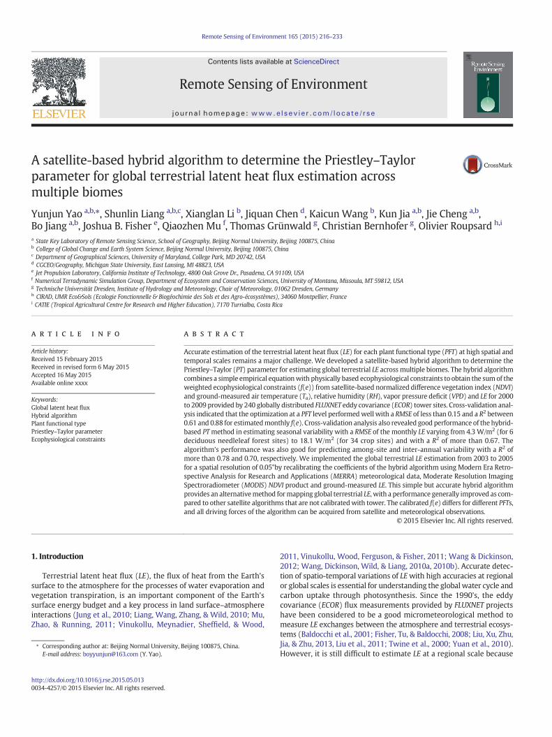
Fig. 3. Scatter plots of the observed monthly f(e) versus f(sm) at the site scale for each PFT. f(e) is inverted from Eq. (3) using ground-measured Rn, LE, Ta and G collected from flux towersites. f(sm) is calculated using RH and VPD collected from flux tower sites.

219Y. Yao et al. / Remote Sensing of Environment 165 (2015) 216–233

of air temperature and physical-based water parameters to estimatef(e).

f e" # ! a0 $ a1 f Ta" # $ a2 f m" # "4#

f m" # ! b0 $ b1 f em" # $ b2 f tm" # $ b3 f ws" # $ b4 f im" # "5#

where ai (i=0,…,2) and bi (i=0,…,4) are the empirical coefficients,f(Ta) is the temperature constraint, and f(m) is the moisture con-straint, which can be considered to be a linear equation of unsaturat-ed soil moisture constraint f(em), vegetation transpiration moistureconstraint f(tm), saturated soil moisture constraint f(ws) and canopyinterception moisture constraint f(im). In our PT algorithm, bothf(ws) and f(im) represent themaximum LEwith sufficient water con-ditions, namely,

f ws" # ! 1 "6#

f im" # ! 1 "7#

f(Ta) for both surface soil and vegetation follows the empirical equa-tion detailed by Wang et al. (2007):

f Ta" # ! c0 $ c1Ta "8#

where ci (i = 0,1) is the empirical coefficient. f(em) is mainly con-trolled by soil moisture. In our algorithm, we chose RHVPD as intro-duced by Fisher et al. (2008) to parameterize f(em) based on thecomplementary hypothesis that surface moisture status is linked to

the evaporative demand (ED) of the atmosphere, indicating thatsoil moisture is characterized by the adjacent atmospheric moisture(Bouchet, 1963; Fisher et al., 2008). Thus, f(em) can be expressed as:

f em" # ! d0 $ d1RHVPD "9#

where di (i=0, 1) is the empirical coefficient. f(tm) is closely relatedto vegetation canopy conductance (gs). According to previous stud-ies, gs mainly depends on photosynthetic leaf area, plant moisture,Ta and VPD (Jarvis, 1976; Mu et al., 2007, 2011; Wang & Dickinson,

Fig. 4. Scatter plots of the observed monthly f(e) versus f(vm) at the site scale for each PFT. f(e) is inverted from Eq. (3) using ground-measured Rn, LE, Ta and G collected from flux towersites. f(vm)= (k3NDVI! k4)VPD, which is calculated usingMODIS NDVI and VPD collected from flux tower sites. Both k3 and k4 of Eq. (11) were calibrated by using linear regression usingthe observed data collected flux tower sites.

Table 1Coefficients derived from global plant functional type-based optimization of Eq. (11) usingMODIS NDVI and tower-specific meteorology. DBF: deciduous broadleaf forest; DNF: decidu-ous needleleaf forest; EBF: evergreen broadleaf forest; ENF: evergreen needleleaf forest; MF:mixed forest; SAW: savannas and woody savannas; SHR: open shrubland and closed shrub-land; CRO: cropland; GRA: grassland, urban and built-up, barren or sparsely vegetated.

Plant functional types Coefficients for different PFTs

k0 k1 k2 k3 k4

CRO 0.2093 0.0024 0.5558 0.1651 0.4860GRA 0.2734 0.0070 0.4556 0.2329 0.4399SAW 0.1749 0.0022 0.4972 0.1573 0.4279SHR 0.2101 0.0061 0.3729 0.1595 0.3102DNF !0.2442 0.0119 0.7722 0.1474 0.5500DBF !0.0456 0.0114 0.5417 0.1510 0.4118MF 0.4968 0.0110 0.0724 0.7139 0.7495EBF 0.2740 0.0047 0.3820 0.1170 0.2190ENF 0.1730 0.0091 0.3680 0.0656 0.0765Average 0.1691 0.0073 0.4464 0.2122 0.4079

220 Y. Yao et al. / Remote Sensing of Environment 165 (2015) 216–233

2012). In our algorithm, we used satellite-based NDVI and VPD toparameterize f(tm), because NDVI, which has no model-relatederrors, is sensitive to LAI, and (e1NDVI ! e2)VPD is used to reducethe maximum gs when VPD is high enough to inhibit photosynthesis(Leuning, 1995; Misson, Panek, & Goldstein, 2004; Mu et al., 2007;Wang et al., 2010a, 2010b; Xu & Baldocchi, 2003), such that:

f tm" # ! e0 $ e1NDVI!e2" #VPD "10#

where ei (i = 0,…,2) is the empirical coefficient. Eq. (10) shows thatf(tm) is diagnosed by the NDVI and VPD terms, and the temperatureterms are directly included in f(e). Combining Eqs. (3)–(10), we sim-plify these empirical coefficients and obtain the hybrid algorithm-based PT equation:

LE ! "Δ

Δ$ #Rn!G" # k0 $ k1Ta $ k2RHVPD $ k3NDVI!k4" #VPD

h i"11#

ki (i=0,…,4) is the empirical coefficient. For simplicity, we assumedthat f(sm) = RHVPD and f(vm) = (k3NDVI! k4)VPD. We also estimat-ed G based on a simple statistical method driven by fractional vege-tation cover (fc) and Rn (Halliwell & Rouse, 1987; Rouse, 1984; Yaoet al., 2013; Zhang et al., 2009):

G ! ag 1! f c" #Rn "12#

f c !NDVI!NDVImin

NDVImax!NDVImin"13#

where ag is a constant (0.18).NDVImax and NDVImin are themaximumand minimum NDVI during the study period and are set as invariantconstants: 0.95 and 0.05, respectively (Tucker, 1979; Zhang et al.,2009). fc will be replaced by one of the satellite products that arebased on more sophisticated estimation algorithms (Jia et al., 2015;Liang et al., 2012).

Advantages offered by the hybrid algorithm-based PT method overother complicated physical LE models are that 1) it is easy to operatefor routine, long-term mapping of LE because it only requires Rn, Ta,NDVI, RH and VPD and avoids wind speed (WS) and soil moisture. Reli-able soil moisture and WSmeasurements that are required to parame-terize LE in many algorithms are unavailable at large scales (Gao &Dirmeyer, 2006;McVicar et al., 2012;Wagner et al., 2003); 2) it reducesthe errors in the required forcing data by avoiding the use of thetemperature or humidity differences and by overcoming use of thecomputational complexities of aerodynamic and surface resistance(Wang & Dickinson, 2012); and 3) it considers the differences in thecoefficients of the Eq. (11) for different PFTs to improve the accuracyof LE estimation.

3.2. Cross validation

The parameters of the Eq. (11) were calibrated by linear regressionusing the observed data (EC ground-measured data and MODIS NDVIproduct) collected from a sufficient number of representative fluxtowers. To validate the estimated f(e) and LE accuracy, we evaluatedthe performance of the satellite-based hybrid algorithm and the corre-sponding PT model using a five-fold cross validations method, whichrandomly stratified the dataset into five groups with approximatelyequal numbers of samples (Jung et al., 2011). We independently vali-dated the estimated LE for each of the five groups based on the calibrat-ed coefficients of Eq. (11), using data from the remaining four groups.We performed the optimizations for the parameters in Eq. (11) foreach PFT. The optimization is based on the least square method to min-imize the difference between the estimated f(e) using satellite and me-teorological forcing data and the observed f(e) inverted from Eq. (3)using ground-observed LE, Ta, Rn and G from flux tower sites. We alsosummarized the squared correlation coefficients (R2), root mean square

error (RMSE), bias and p values of the estimated f(e) and LE and thosederived from the flux tower data to demonstrate the relative predictiveerrors.

To evaluate the ability of our method to predict the spatio-temporalvariations in LE, we used the observed and estimated data to test threecategories of LE variability: (1) seasonal variation, (2) among-site varia-tion, and (3) annual anomalies. We first performed a series of cross-validations of LE seasonal cycle by comparing the daily (monthly) esti-mated LE and the observed LE. To test the among-site variation, we val-idated the average values of the measured and predicted LE at each siteover the entire period. To assess howwell themodel predicts long-termvariations in LE, we averaged themeasured andpredicted LE into annualvalues at each site and removed the multiyear average from the annualvalues to acquire annual LE anomaly for each site. We chose flux towersites that had at least three years' worth of data.

For comparisonwith LE estimates based on the other algorithms, weused a simple holdout method that randomly divided the dataset intotwo groups with approximately equal numbers of samples (Yao, Liang,Li, et al., 2014). We validated daily LE using data from the first group

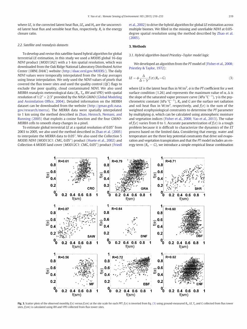
Fig. 5. Sensitivity of f(e) to variations in the amounts of a) Ta (RH=0.7,NDVI=0.7), b)RH(Ta=25 °C,NDVI=0.7) and c)NDVI (Ta=25 °C, RH=0.7). Other input variables are setas constants when one variable changes.

221Y. Yao et al. / Remote Sensing of Environment 165 (2015) 216–233

based on the calibrated coefficients of Eq. (11) using data from thesecond group andwe then validated daily LEusing data from the secondgroup based on the calibrated coefficients of Eq. (11) using data fromthe first group.

3.3. Comparison with other LE algorithms

3.3.1. MOD16 LE algorithmAMOD16global LE retrieval algorithm is based on thewell-established

Penman–Monteith logic (Monteith, 1965) with modifications to accountfor parameters not readily available from space (Cleugh et al., 2007).TheMOD16 algorithm accounts for both surface energy partitioning andenvironmental constraints on ET, and includes canopy interception evap-oration, evaporation from wet/moist soil surfaces, and transpirationthrough vegetation pores (stomata). Atmospheric relative humidity(RH) is used to quantify the proportion of wet soil and wet canopy com-ponents (Fisher et al., 2008). Proportional vegetation cover is derivedfrom MODIS fractional absorbed photosynthetically active radiation(FPAR) (Los et al., 2000), and used to partition net radiation (Rn) betweenvegetation and soil surfaces. Leaf level stomatal conductance is deter-mined by the mean daytime surface air vapor pressure deficit (VPD)and daily minimum air temperature (Tmin), and further up-scaled to thenon-wet canopy level using the MODIS leaf area index (LAI) product(MOD15A2). Using the complementary relationship hypothesis (Fisheret al., 2008), soil evaporation is estimated as the potential evaporationrate for wet soil surfaces scaled down by RH and VPD formoist soil condi-tions. The daily LE calculation represents the 24 h sumof LE from the day-time and nighttime (largely minimal) calculations. MOD16 LE algorithmwas validated at 46flux tower sites and agreedwith the LEmeasurements

well (Mu et al., 2011). Considering that most LE occurs during daytime,our proposed PT algorithm in this study only estimated daytime LE andneglected nighttime LE. Therefore, we only used MOD16 algorithm toestimate daytime LE.

3.3.2. PT-JPL LE algorithmA Priestley–Taylor-based (PT-JPL) LE algorithm was introduced by

Fisher et al. (2008), based on the PT equation to downscale potentialLE to actual LE by adding both atmospheric (RH and VPD) and ecophys-iological constraints (FPAR and LAI). PT-JPL estimates LE by calculatingthe sum of the soil evaporation, the canopy transpiration and the cano-py interception evaporation. The validation at the 39 global flux towersites illustrates that the averaged RMSE of the estimated and observedLE is 15.2 W/m2 with an R2 of 0.9 (Fisher et al., 2008, 2009). PT-JPL hasbeen independently demonstrated as the highest performing physicallybased global remote sensing LE algorithm in multi-algorithm intercom-parisons (Chen et al., 2014; Ershadi et al., 2014; Vinukollu, Meynadier,et al., 2011; Vinukollu, Wood, et al., 2011).

4. Results

4.1. Optimization of the PT parameter

To parameterize the PT parameter, we used f(e) to replace the orig-inal PT parameter because f(e) is a suitable ecophysiological index forthe temporal scaling. To determine the factors that drive the variationof f(e), we analyzed the variations of the combined variables fromground-measured Ta, RH, VPD and MODIS NDVI from all of the fluxtower sites. Fig. 2 gives an example of the temporal variation of the

Fig. 6. Cross-validation of the estimated monthly f(e) using the hybrid algorithm driven by tower-specific meteorology versus ground-measured f(e) for each PFT.

222 Y. Yao et al. / Remote Sensing of Environment 165 (2015) 216–233

8-day f(e) estimated directly from observations during January2002–December 2006 at the Au-How site using Eq. (3) togetherwith Ta, f(sm) and f(vm). Both f(sm) and f(vm) have an obvious sea-sonal pattern in this savanna that was similar to f(e) and have highcorrelations with f(e) at all of the flux tower sites. Although thevariation of Ta also follows that of Ta, Ta has a relatively lower corre-lation with f(e) at all of the flux tower sites because Δ/(Δ + #)

directly included Ta. Therefore, soil moisture and vegetation moisturewere the largest contributors to the variations in f(e).

Figs. 3 and 4 show the correlations of monthly observed f(e) directlyinverted from observations using Eq. (3) with monthly f(sm) and f(vm)for different biomes, respectively. Generally speaking, variations inmonthly f(sm) explained 25% to 82% of the variance in monthly f(e) atall sites. The correlation coefficients between f(e) and f(sm) vary from

Daily Monthly Among sites Annual Anomalies

CR

OG

RA

SH

RS

AW

DN

FD

BF

Fig. 7. The estimated LE (y axis, unit:W/m2) using our PT algorithm driven by tower-specificmeteorology versus ground-measured LE (x axis, unit:W/m2) for cross validation for daily LE,monthly LE, among-sites variability and annual LE anomalies.

223Y. Yao et al. / Remote Sensing of Environment 165 (2015) 216–233

0.56 (p b 0.01) at all MF sites to 0.87 (p b 0.01) at all SAW sites. Thecorrelations between f(e) and f(sm) in both all GRA and SAW sites arehigher than 0.78 (p b 0.01), yet f(sm) was not always the best predictorof f(e) in the CRO and forest (excluding EBF) ecosystems. Therefore,f(sm) captures the variations in surface soil evaporation for differentPFTs because surface soil moisture can sustain the transpiration ofsparse vegetation (e.g., grass and savanna) and cannot provide supplywater for the transpiration of dense vegetation (e.g., forests). As expect-ed, f(vm) also explains much of the variance of f(e) in most obvious

seasonal biomes, and f(vm) is highly correlated with f(e) for deciduousforests, shrub, crop and grass sites. For instance, the correlation coefficientbetween f(vm) and f(e) is 0.89 (p b 0.01) at all DNF sites and 0.78(pb 0.01) at all SHR sites. Thus, f(vm) characterizes the vegetation transpi-ration across multiple biomes by a combination of NDVI and VPD becauseNDVI is used to monitor the seasonal variation of vegetation growth andVPD reflects the negative effects of vegetation photosynthesis.

Table 1 shows the parameters of Eq. (11) for nine different biomes bylinear regression based on the satellite-based NDVI, ground-measured Ta,

Daily Monthly Among sites Annual Anomalies

MF

EB

FE

NF

All

Fig. 7 (continued).

Table 2A summary of the statistics (bias, the root mean square error, RMSE, and the square of the correlation coefficients, R2) of the comparison between the ground-measured and the estimatedaverage daily LE using the three LE algorithms driven by tower-specific meteorology of the first group. The second group was used as training data to calibrate the coefficients of our PTalgorithm. The bias and RMSE are in units of W/m2. PT-hybrid stands for our PT algorithm.

PFTs Bias RMSE R2

MOD16 PT-JPL PT-hybrid MOD16 PT-JPL PT-hybrid MOD16 PT-JPL PT-hybrid

DBF !10.2 9.8 5.4 28.7 27.1 21.6 0.61 0.73 0.79DNF !9.1 5.4 3.3 21.2 19.2 12.9 0.42 0.65 0.81EBF !6.3 18.7 2.8 27.6 34.3 23.4 0.57 0.58 0.69ENF !5.5 13.1 2.1 30.5 31.2 22.8 0.42 0.64 0.66MF !6.7 5.8 3.4 27.4 28.1 20.4 0.48 0.72 0.80SAW !8.2 11.3 5.2 25.9 22.3 19.7 0.47 0.53 0.71SHR !1.8 8.6 4.6 26.1 22.8 16.8 0.41 0.59 0.63CRO !12.6 !2.3 6.5 32.3 25.3 21.1 0.52 0.68 0.77GRA !9.2 1.8 4.3 26.9 19.8 18.7 0.50 0.70 0.76Average !7.7 8.0 4.2 27.4 25.6 19.7 0.50 0.64 0.74

224 Y. Yao et al. / Remote Sensing of Environment 165 (2015) 216–233

RH, VPD and f(e). Our proposed hybrid algorithm yields different values off(e) for each PFT. For example, in July, GRA and CRO had the largest esti-mated f(e) (approximately 0.85), followed by DNF, DBF, SAW, EBF, SHR,while ENF andMF had the minimum f(e). f(vm) by integrating NDVI andVPD is highly correlated to LE in all biomes and f(e) increased as a functionof f(vm) with vegetation growth. f(sm) affected f(e) significantly for non-forests, and LE for forests was not dependent on surface moisture.

The sensitivity experiments used to determine the dependence off(e) on Ta, RH and NDVI are shown in Fig. 5. The f(e) at different biomesvary by less than 0.3 with the increasing Ta from 5 to 30 °C when otherinput variables are set as constants (RH=0.7; NDVI=0.7). In responseto the same changes in Ta, the estimated f(e) at the DNF sites varies themost comparedwith those at other biome sites. Similarly, the estimatedf(e) varies by less than 0.5 for a 0.8 change in RH and NDVI at most PFTsites. However, at MF sites, f(e) increase by more than 0.5 for a 0.8 in-crease in RH and NDVI. Therefore, both RH and NDVI have a significantinfluence on f(e), and f(e) is less sensitive to the error in Ta but cannotbe neglected.

4.2. Algorithm evaluation

4.2.1. Algorithm performance based on cross validationWe performed a series of cross validations to evaluate the perfor-

mance of our satellite-based algorithm for monthly f(e) at differentPFTs. Fig. 6 shows the comparison of estimated and observed monthlyf(e) at nine biomes. It is clear that the performance varies with thebiomes and criteria (bias, RMSE and R2). The RMSE between estimatedf(e) and observed f(e) are all less than 0.15, and the R2 ranges from0.61 to 0.88 (99% confidence). The hybrid algorithmhas the highest per-formance, with an RMSE of 0.07 and an R2 of 0.86 (p b 0.01) at the DNFsites, followed by at SAW, SHR, GRA, DBF, EBF,MF and CRO sites. Howev-er, the worst performances, with an R2 of 0.55 (p b 0.01), occur at theENF sites. In general, the few samples at the DNF sites led to the relativehigher accuracy of f(e) estimation. Perhaps when there are equal num-bers of samples at the different biomes, the algorithm will have loweraccuracy of f(e) at dense forest sites due to the saturation effect ofNDVI. We consider that the overall performance of our algorithm atdifferent PFTs is satisfying for estimating the PT parameter.

Estimated LE based on our PTmodel driven by tower-specific mete-orology and MODIS NDVI product was also cross-validated. A compari-son of the measured and estimated daily (monthly) LE at the site scalefor each PFT demonstrates that our PT algorithm accurately estimatesseasonal LE (Fig. 7). At the PFT level, the RMSE of the estimated monthly(daily) LE varies from 4.3 (11.5) W/m2 for all DNF sites to 18.1 (20.9)W/m2 for all CRO sites and the R2 (99% confidence) varies from 0.80(0.68) for all SHR sites to 0.96 (0.87) for all DNF sites. The seasonal varia-tion of LE is the most robust feature using both daily and monthly ECORdata. In Fig. 7 we can also observe a good ability of our PT algorithm toestimate the among-site variability, where the R2 of the site-averagedestimated versus observed LE ranges from 0.78 (p b 0.01) for all GRAsites to 0.96 (p b 0.01) for all DNF sites and the RMSE varies from2.1 W/m2 for all SHR sites to 9.5 W/m2 for all SAW sites. Overall, theestimated LE based on our algorithm displays a high accuracy accordingto the validation of seasonal and spatial variation in LE. Clearly, our algo-rithm is also satisfactory in reproducing the inter-annual variability atthe site scale for each PFT with at least 3 years of data (Fig. 7). The R2

between themeasured and estimated annual LE anomaly is significantlybelow the confidence level of p b 0.05 and is between 0.71 for all ENFsites and 0.94 for all DNF sites. The lowest RMSE is 2.1 W/m2 at all DNFsites due to the few samples, while the largest RMSE is 5.8 W/m2 at allEBF sites due to the missing observed LE data caused by bad weatherconditions in tropical ecosystems (Falge et al., 2001).

4.2.2. Comparison with other LE algorithmsBecause point-based validation with ground observation is typically a

good method to evaluate algorithm performance (Vinukollu, Meynadier,

et al., 2011; Vinukollu, Wood, et al., 2011), the estimated daily LE at sitescale using our PT algorithm was compared with those for the MOD16algorithm and the PT-JPL algorithm for each PFT. Table 2 shows the resultsof comparisons between the estimated LE using the three algorithmsversus daily ground-observations from the first group using the secondgroup data to calibrate the coefficients of our PT algorithm. For CRO andGRA sites, the average RMSE of the estimated LE using our algorithm isless than 22 W/m2, and the average R2 is more than 0.75 (p b 0.01),which show better performance than the MOD16 algorithm and the PT-JPL algorithm. For all forests sites, the average RMSE of the estimated LE

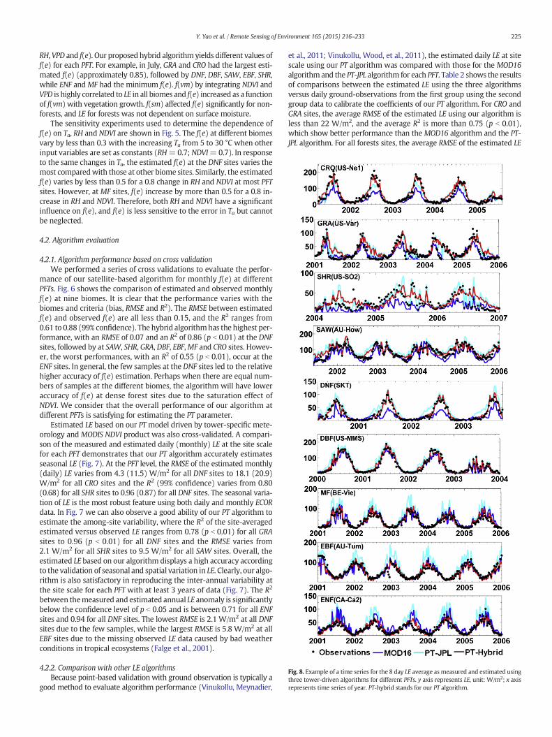
Fig. 8. Example of a time series for the 8 day LE average as measured and estimated usingthree tower-driven algorithms for different PFTs. y axis represents LE, unit: W/m2; x axisrepresents time series of year. PT-hybrid stands for our PT algorithm.

225Y. Yao et al. / Remote Sensing of Environment 165 (2015) 216–233

using our PT algorithm is less than 24 W/m2 and is lower than for theMOD16 algorithm and the PT-JPL algorithm together with slightly higherR2 at the 99% level of confidence. For the SHR and SAW sites, the averageRMSE of the estimated LE using our PT algorithm is much lower and theaverage R2 is more than 0.62 (95% confidence) when compared withthe other two algorithms. Overall, the average RMSE for our PT algorithmdecreased by approximately 5 W/m2 for forests and SHR sites, and ap-proximately 3 W/m2 for CRO and SAW sites, and approximately 2 W/m2

for GRA sites. The average R2 increases by approximately 0.1 (p b 0.05)at SAW and CRO sites and, by approximately 0.06 (p b 0.05) atmost forest,SHR and GRA sites. This improvement overMOD16 and PT-JPL is expectedgivenour calibration to ECORdata,withwhichwe also used for validation.

Fig. 8 shows a time series for 8-day average LE measurements andtower-driven predictions for PFTs. In comparison to the MOD16 algo-rithm and the PT-JPL algorithm, in this study our PT algorithm yieldedseasonal LE variations that are closest to the ground-measured values.Table 3 presents the statistics of the comparisons of the three LE algo-rithms from the second group, using the first group data to calibratethe coefficients of our algorithm, and we draw the similar conclusionthat our proposed LE algorithm presents better performance for quanti-fying the turbulent heat fluxes than that of the MOD16 algorithmand the PT-JPL algorithm. Therefore, our PT algorithm is among thosealgorithms that provide a better fit to flux tower observations.

4.3. Global implementation of the terrestrial LE estimation based onMERRAdata

Based on Eq. (11) parameterized by the coefficients listed in Table 1,we estimated global terrestrial LE during 2000–2009 with a spatialresolution of 0.05° using MERRA meteorological data and MODIS prod-ucts. Unfortunately, we found that our PT algorithm tends to underesti-mate LE usingMERRA data when compared to ground-measured LE dueto the underestimated Rn from MERRA data (Fig. 9). To improve the

accuracy of the estimated LE driven by MERRA data, we recalibratedthe coefficients of Eq. (11) using the MERRA meteorological data,MODIS products and ground-measured LE collected at global-distributed flux tower sites. Table 4 lists the parameters of Eq. (11) fornine different biomes by linear regression based on the MODIS-derived NDVI, ground-measured f(e), MERRA-derived Ta, RH and VPD.Cross-validations show that when using MERRA data as a substitutefor tower-specific meteorology, our revised PT algorithm driven byMERRA data produced higher predictive errors at most flux towersdue to the large errors of MERRA meteorological data. The averageRMSE of the daily LE increased from 18.2 W/m2 using the original algo-rithm driven by specific-tower meteorology to 20.6 W/m2 using therevised algorithm driven by MERRA data (Fig. 10). The coefficient ofdetermination (R2) between the daily LE estimates and observationsdecreased from 0.84 using the original algorithm to 0.70 using therevised version. Predicted relative errors of LE for MERRA-based revisedalgorithm compared to the original version also slightly increased by 4%for validating among-sites variability and annual LE anomalies. Wanget al. (2010a) suggested that the relative error of the required LE simula-tion for analyzing spatiotemporal variation is typically less than 14% andthe accuracy of our revised algorithm driven by MERRA data meets thisrequirement.

We evaluated the global spatial patterns of f(e) and LE averaged from2003 through 2005 usingmonthlyMERRA gridded data. Tropical rainfallforests in the Amazon regions of South America, Congo basins of Africaand the Southeast Asia and European monsoonal temperate regionshad the highest annual f(e). Arid regions and the Arctic had the lowestannual f(e) due to the contribution of low soil moisture and vegetationcover to decreasing LE. Global annual f(e) varies from 0.22 in barrenlands, 0.42 in SHR, 0.51 in GRA, 0.65 in CRO, 0.66 in DBF, to 0.73 in EBF(Fig. 11).

Global annual LE is 41.7 W/m2 over vegetated regions. The highestannual LE is found in the equatorial tropics and monsoonal subtropical

Table 3A summary of the statistics (bias, the root mean square error, RMSE, and the square of the correlation coefficients, R2) of the comparison between the ground-measured and the estimatedaverage daily LE using the three LE algorithms driven by tower-specific meteorology of the second group. The first group was used as training data to calibrate the coefficients of our PTalgorithm. The bias and RMSE are in units of W/m2. PT-hybrid stands for our PT algorithm.

PFTs Bias RMSE R2

MOD16 PT-JPL PT-hybrid MOD16 PT-JPL PT-hybrid MOD16 PT-JPL PT-hybrid

DBF !12.6 6.2 4.7 33.2 30.3 24.3 0.57 0.62 0.78DNF !7.5 9.2 7.2 26.3 27.8 19.4 0.45 0.49 0.59EBF !12.6 14.8 1.2 37.2 39.8 31.8 0.41 0.42 0.62ENF !5.3 7.4 2.8 28.1 23.8 20.7 0.45 0.59 0.79MF !1.7 10.2 4.6 27.3 27.1 21.9 0.51 0.65 0.81SAW !18.9 6.1 1.1 30.7 27.5 20.6 0.41 0.51 0.61SHR !2.2 9.3 1.2 26.6 23.8 18.1 0.41 0.52 0.59CRO !14.3 !1.8 3.8 34.8 30.8 29.5 0.42 0.51 0.63GRA !7.3 5.2 3.9 28.8 26.6 23.4 0.41 0.52 0.60Average !9.1 7.4 3.4 30.3 28.6 23.3 0.45 0.54 0.67

Fig. 9.Anexample of a) comparison of daily LEobservations atUS-Wcr site and the corresponding estimated LEbased on Eq. (11)with the coefficients listed in Table 1 drivenby theMERRAdataset. b) Comparison of daily Rn observations at US-Wcr site and the corresponding Rn derived from MERRA dataset.

226 Y. Yao et al. / Remote Sensing of Environment 165 (2015) 216–233

regions due to the sufficient soil moisture and higher vegetation cover.Small LE occurs in cold and dry environments due to the lower temper-ature and precipitation. EBF has the largest average LE (90.9 W/m2),followed by SAW (70.3 W/m2), DBF (61.2 W/m2), CRO (46.2 W/m2), MF(37.3 W/m2), GRA (31.9 W/m2), ENF (27.5 W/m2), SHR (19.6 W/m2)and DNF (18.8 W/m2) (Fig. 12).

5. Discussion

5.1. Ecophysiological hypothesis for optimization of the PT parameter

The basis of PT models is the hypothesis that the energy termscoupled with the ecophysiological constraints are the main controllerof LE and determine the partition of the sensible and latent heat flux(Jarvis & Mcnaughton, 1986; Priestley & Taylor, 1972). In the satellite-based PT algorithms, ecophysiological constraints are recognized asthe core regulators for downscaling potential LE to actual LE. For unsat-urated soil and vegetation surfaces where there is limited supply of soilmoisture, ecophysiological constraints and LE are affected significantlyby available water and canopy structures (Baldocchi & Xu, 2007;Davies & Allen, 1973; Jin et al., 2011; Komatsu, 2003). f(e) used in thisstudy includes the variables (f(sm) and f(vm)) for characterizing avail-ablewater and vegetation information, all ofwhich can be fully acquiredfrom satellite data.

Several studies have suggested using satellite-derived soil moisturewith a high spatial heterogeneity to parameterize the soil moistureconstraint for estimating soil evaporation (Gokmen et al., 2012; Jinet al., 2011; Miralles et al., 2011). However, satellite-derived soil mois-ture only considers surface soil moisture from approximately the top2–5 cm of the soil profile and neglects the moisture deeper within thesoil profile (Anderson, Norman, Mecikalski, Otkin, & Kustas, 2007;Jarvis, 1976). In general, soil evaporation stems from the contributionsof soil moisture from all of the different layers of the soil profile. Intheory, by combining RH and VPD, f(sm) used in this study couples theentire atmosphere boundary layer and soil evaporation to characterizethe atmospheric evaporative demand and hydrological effects on soilmoisture diffusion through different soil layers, even though f(sm)may not explicitly represent the soil water deficit on daily scales whenconvection is frequent and strong due to strong vertical mixing (Fisheret al., 2008; Salvucci & Gentine, 2013). Previous studies have usedf(sm) to calculate soil water deficit and neglected their differences indifferent biomes (Fisher et al., 2008; Mu et al., 2011). However,our algorithm accounts for their differences using f(sm) multipliedwith different coefficients. VPD-based algorithm maintains a physi-cally realistic representation of soil evaporation and is operational toreplace soil moisture-based methods, especially when soil moisture isnot available.

In this study, the nonlinear algorithmof f(vm), defined as a function ofNDVI and VPD, represents an improvement for optimizing PT parameterbecause it expresses the canopy-level transpiration rate by coupling

vegetation water supply with atmospheric evaporative demand. Thedecrease of NDVI and LAI respond to the rise in vegetation water stressand stomatal closure by altering their leaf density to adapt to the changingenvironment (Field, Randerson, & Malmstrom, 1995; Gokmen et al.,2012). NDVI was chosen to substitute LAI because LAI will overestimatevegetation canopy conductance when LAI is higher than 3 (Glenn,Huete, Nagler, Hirschboeck, & Brown, 2007; Suyker & Verma, 2008). The(e1NDVI! e2)VPD term considers the effect of causing f(e) for differentbiomes to level off in tropic regions with low VPD and highly saturat-ed NDVI values. Although f(e) or EF are more linearly related to NDVI(Choudhury, Ahmed, Idso, Reginato, & Daughtry, 1994; Wang et al.,2007), our satellite-based hybrid algorithm to determine the PTparameter yields comparable results.

5.2. Algorithm performance analysis

Algorithm calibration and validation at 240 globally distributedECOR flux tower sites illustrates that the satellite-based hybrid algo-rithm for estimating f(e) and LEwas reliable and robust across multiplebiomes and different climate regions. Figs. 6 and 7 demonstrate that thesatellite-based hybrid algorithm yielded small errors of f(e) and LEacross multiple biomes based on the cross-validations. However, thehybrid algorithm still has relatively low R2 and large RMSEs for the esti-mated f(e) and LE compared to ground-measured data at some irrigatedcrop sites. This suggests that irrigation and fertilization practices, and ingeneral differences among crop types,may bemore critical than canopystructure in determining PT model performance (Zhang et al., 2012).When excluding the observations of these irrigated crop sites, thehybrid algorithm performance greatly improved.

Under the samemeteorological and ecological conditions, the hybridalgorithm and PTmodel had large inter-biome differences for predictivef(e) and LE. For instance, the hybrid algorithm yielded the high f(e)values (more than 0.75 under ideal conditions) and explained morethan 80% of the f(e) variability for GRA, non-irrigated crop, DNF andDBF sites (Fig. 13). Many studies have demonstrated that these PFTspresent strong seasonal changes in vegetation leaf, chlorophyll contentand red reflectance (Mu et al., 2007; Yan et al., 2012; Yao, Liang, Li, et al.,2014; Yao, Liang, Xie, et al., 2014, Yebra, Van Dijk, Leuning, Huete, &Guerschman, 2013). Satellite-based NDVI responds strongly to varia-tions in red reflectance, chlorophyll and LAI variations as vegetationleaf dries in many vegetation species. Our hybrid algorithm capturesthis seasonal cycle of vegetation to improve the accuracy of estimatingf(e) and LE by using NDVI to parameterize f(vm). In contrast, the hybridalgorithm yielded the poor performances for f(e) (RMSE " 0.09,R2 b 0.65) and LE (RMSE " 17.5 W/m2 and R2 b 0.80) estimates forsite-specific meteorology inputs for ENF and EBF sites. For tall ENF andEBF regions, vegetation seasonal variations are less evident, and NDVIsaturates and is contaminated by clouds, which reduces the ability off(e) to reliably capture satellite signals of vegetation transpiration(Huete et al., 2002). This hypothesis is supported by the previousstudy of Eugster et al. (2000), which reported that evergreen coniferforests have a canopy conductance that is half that of deciduous forests,which is consistentwith our finding that our hybridmethod yielded thelowest f(e) for evergreen forests under the same meteorological andeco-physiological conditions (Fig. 13). Direct evidence of this interpre-tation is that the availability of f(sm) to resolve changes in f(e) and LEin this land functional type is limited, with an R2 of 0.34 (p b 0.05) dueto the lower bare soil exposure ratio caused by greater overlapping ofleaves of different species competing for sunlight (Eugster et al., 2000).

A typical difference between our PT algorithm and other two algo-rithms (PT-JPL and MOD16) is that our algorithm combines ground-observations and physically based ecophysiological constraints toparameterize f(e) for each PFT. Although our algorithm uses a relativelysimple and largely empirical equation of the LE process, it has loweruncertainties in the required forcing data and illustrates the improvedperformance compared to other two algorithms. Moreover, a resistance-

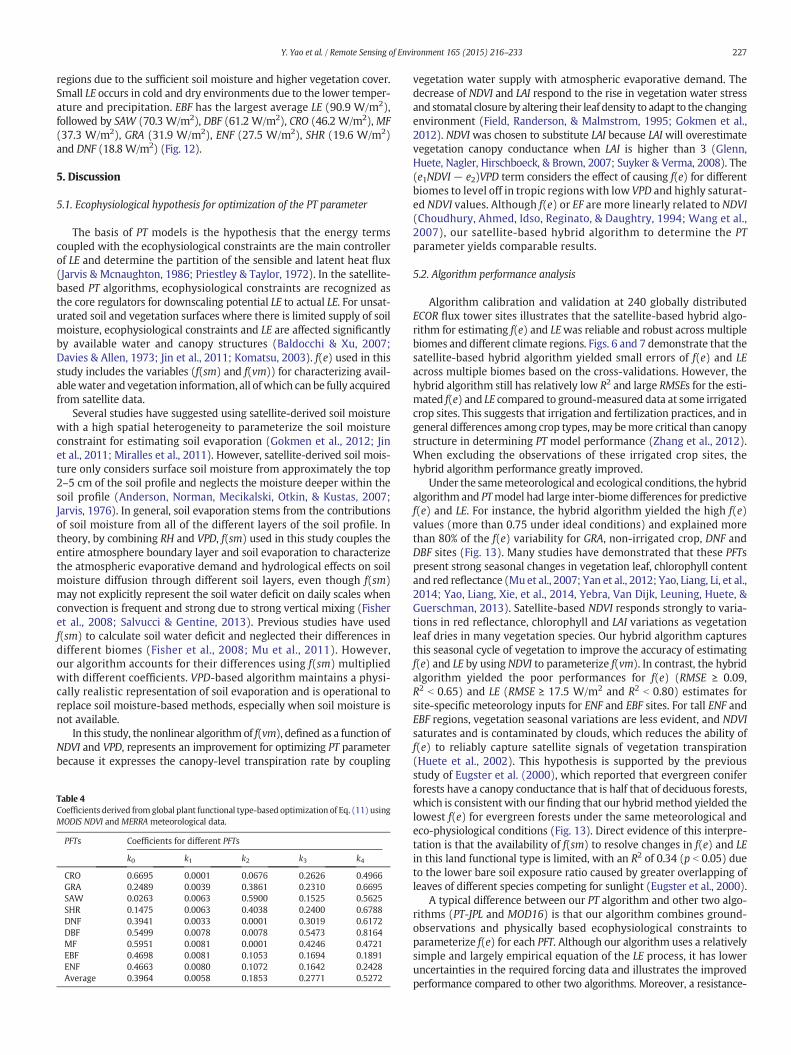
Table 4Coefficients derived from global plant functional type-based optimization of Eq. (11) usingMODIS NDVI andMERRAmeteorological data.

PFTs Coefficients for different PFTs

k0 k1 k2 k3 k4

CRO 0.6695 0.0001 0.0676 0.2626 0.4966GRA 0.2489 0.0039 0.3861 0.2310 0.6695SAW 0.0263 0.0063 0.5900 0.1525 0.5625SHR 0.1475 0.0063 0.4038 0.2400 0.6788DNF 0.3941 0.0033 0.0001 0.3019 0.6172DBF 0.5499 0.0078 0.0078 0.5473 0.8164MF 0.5951 0.0081 0.0001 0.4246 0.4721EBF 0.4698 0.0081 0.1053 0.1694 0.1891ENF 0.4663 0.0080 0.1072 0.1642 0.2428Average 0.3964 0.0058 0.1853 0.2771 0.5272

227Y. Yao et al. / Remote Sensing of Environment 165 (2015) 216–233

based PM algorithm is not accurate to calculate canopy resistance indiverse vegetation, and the structure of the PT-JPL algorithm by designignores classifications among PFTs (Ershadi et al., 2014; Fisher et al.,2009).

The accuracy of our algorithm is highly dependent on the accuracy ofthe ECOR LE ground-measurements, algorithm input errors (including PFTclassification map), spatial scale mismatches among different datasetsand algorithm inherent limitations. Although ECOR measurements are

relatively accurate, they have an error of approximately 5–20% (Foken,2008; Glenn et al., 2008) and the gap filling from days to months alsoleads to 5% errors for annual values of LE (Hui et al., 2004). Addition-ally, ECOR measurements have an energy imbalance problem, withH+ LE b Rn! G (Wilson et al., 2002), and the annualmean energy bal-ance closure at more than 200 FLUXNET sites was approximately 0.8(Beer et al., 2010). Although several reasons for this energy closureproblem have been documented by a substantial body of literature

Daily Monthly Among sites Annual anomalies

CR

OG

RA

SH

RS

AW

DN

FD

BF

Fig. 10. The estimated LE (y axis, unit:W/m2) using our PT algorithmdriven byMERRAmeteorological data versus ground-measured LE (x axis, unit:W/m2) for cross validation for daily LE,monthly LE, among-sites variability and annual LE anomalies.

228 Y. Yao et al. / Remote Sensing of Environment 165 (2015) 216–233

Daily Monthly Among sites Annual Anomalies

MF

EB

FE

NF

All

Fig. 10 (continued).

Fig. 11. Spatial distribution of annual global terrestrial f(e) averaged for 2003–2005 at spatial resolution of 0.05° according to the satellite-based hybrid algorithm driven byMODIS NDVIand MERRA meteorology.

229Y. Yao et al. / Remote Sensing of Environment 165 (2015) 216–233

(Foken, 2008; Twine et al., 2000; Wang & Dickinson, 2012) and wecorrected it in this study, the errors produced by the correction andmeasurements are still unclear (Shuttleworth, 2007). Moreover, thebiases of other ground-measured meteorological variables (e.g., Ta,RH) also introduced point-based f(e) and LE estimation errors. Whenglobal terrestrial LE was calculated, driven by the MERRA reanalysisdataset, the biases of the MERRA data influenced the accuracy of ouralgorithm, even though we performed a recalibrated measurementusing Eq. (11). Recent studies have revealed substantial errors forMERRA data when compared to ground measurements (Rienecker et al.,2011; Zhao, Running, & Nemani, 2006). In this study, we also found thatMERRA data usually underestimated Rn at high values compared to theground-measurements (Fig. 9). Our algorithm shows significant differ-ences in LE estimation if the classification shifts or iswrong. Previous stud-ies revealed that the accuracy of the IGBP layer of theMODIS Collection 5Land Cover Type product (MCD12Q1) is estimated to be 74.8% globally(Bartholome & Belward, 2005; Friedl et al., 2002; Hansen, Defries,Townshend, & Sohlberg, 2000). Thus, misclassification of the MODISland cover product will also lead to the use of incorrect parameters inEq. (11), resulting in less accurate LE estimates.

Typically, the footprints of the ECORmeasurements are approximatelyseveral hundred meters (Baldocchi, 2008), and the resolutions of bothMODIS NDVI (1 km and 0.05°) and MERRA gridded data (1/2 # 2/3°) aregreater than the footprints of the ECOR measurements (Rienecker et al.,2011). The MODIS NDVI and MERRA gridded meteorological data maynot adequately capture vegetation and eco-physiological signals at theflux tower sites (Mu et al., 2011; Zhang et al., 2010). Inaccurate represen-tations of the field measurement footprint may result in algorithm errors

for many flux tower sites. The structure of our algorithmwill also reducethe accuracy of LE estimates because it ignores the effects of CO2 andWS.High-CO2-induced partial stomatal closure causes an underestimation ofdaily LE when NDVI tends to increase (Idso & Brazel, 1984; Yao et al.,2013). Our algorithm excludesWS becauseWS is not globally observable.By quantifying the sensitivity of wind speed to evaporative demand, arecent study revealed thatWS contributed substantially to declining evap-oration rates (McVicar et al., 2012). For less than twodecades, the effect ofWS on LEmay be negligible, but for several decades, this effect should beconsidered.

5.3. Global terrestrial LE estimation

Despite the existing errors, our proposed algorithm demonstratedits reliability for calculating annual LE, which was compared withother reanalysis, satellite and hydrological datasets. We estimated thatthe annual global terrestrial LE (excluding Greenland and Antarctica)was 41.7 W/m2 during 2003–2005, which is slightly larger than thevalue of independent global estimates: 35.3 W/m2 from a MODIS prod-uct (Mu et al., 2011), 34.2W/m2 fromGSWP data (Dirmeyer et al., 2006)and 40.2 W/m2 based on the Atmospheric Water Balance (AWB) meth-od (Mueller et al., 2011). However, recent studies have demonstratedthat the global average LE derived from multiple algorithms variesfrom 34.1 W/m2 to 42.7 W/m2, with an average of 36.9 W/m2 (Wang

Fig. 12. Spatial distribution of annual global terrestrial LE averaged for 2003–2005 at spatial resolution of 0.05° according to our PT algorithm driven by MODIS NDVI and MERRAmeteorology.

Fig. 13. Variability of f(e) at multiple biomes using the same inputs (Ta = 25 °C, RH= 0.7and NDVI = 0.7).

Fig. 14. Comparison of our LE estimates and MODIS-LE product at the various ecosystemtypes. PT-hybrid stands for our PT algorithm.

230 Y. Yao et al. / Remote Sensing of Environment 165 (2015) 216–233

& Dickinson, 2012). Our estimated annual LE falls within the aboverange.

The global magnitude of LE for each PFT agreed, in general, withresults documented in the literature (Giambelluca et al., 2009; Muet al., 2011; Zhang et al., 2010; Zhang et al., 2009). We found that EBF,SAW, DBF and CRO have the largest annual average LE, greater than45 W/m2, and both SHR and DNF have the lowest annual average LE,less than 20 W/m2, which are in good agreement in its representationof AVHRR-LE (Zhang, Kimball, et al., 2010; Zhang et al., 2010) andMODIS-LE (Mu et al., 2011). Fig. 14 shows the MODIS LE product andour estimates aggregated for vegetation types. In addition, Frank andInouye (1994) estimated annual LE at 94 sites covering 11 biomesbased on approximately 20 years of meteorological records and foundthat the value of annual LE was approximately 15.7 W/m2 for tundra,29.6 W/m2 for taiga, 45.7 W/m2 for broadleaf forests, 68.8 W/m2 forsavannas and 106.1 W/m2 for wet tropical forests. Giambelluca et al.(2009) used ECOR observations to document that the annual averagedLE is 64.1 W/m2 and 53.6 W/m2 for two tropical savanna sites inBrazil. These comparable results demonstrate the applicability of ouralgorithm to accurately estimate global terrestrial LE.

6. Conclusions

We developed a satellite-based hybrid algorithm to calibrate ECORmeasurements to determine the PT parameter for global terrestrial LEestimation across multiple biomes by combining a simple empiricalequation with physically based ecophysiological constraints to obtainthe sum of the weighted ecophysiological constraints (f(e)) from globaleddy covariance, satellite and meteorological observations. f(e) con-siders the differences in coefficients among PFTs and it includes VPD-based soil moisture and NDVI-based vegetation factors. The parametersof the hybrid algorithm for nine different biomes are acquired by linearregression based on the satellite-based NDVI, ground-measured LE, Ta,RH, and VPD. It has a low sensitivity to errors in the input data.

A series of cross-validations based on 240 global ECOR observationsshow that the optimization at a PFT level performed well. The satellite-based hybrid algorithm had the highest performance, with an RMSE of0.07 and an R2 of 0.86 (p b 0.01) at DNF sites, and the worst perfor-mances, with an R2 of 0.55 (p b 0.01), occurred at ENF sites. Cross-validationswere also performed to evaluate the ability of our PTmethodto yield LE seasonal, spatial, and inter-annual variability. On average, theRMSE of the estimated monthly (daily) LE varies from 4.3 (11.5) W/m2

for all DNF sites to 18.1 (20.9) W/m2 for all CRO sites, and the R2 (99%confidence) varies from 0.80 (0.68) for all SHR sites to 0.96 (0.87) forall DNF sites. Performance was also good for predicting among-sitevariability, with an R2 of more than 0.78. The validation of inter-annual variability at the site scale shows that the R2 between the mea-sured and estimated annual LE anomaly is between 0.71 for all ENFsites and 0.94 for all DNF sites. When compared with the MOD16 andPT-JPL algorithms, which are not calibrated to sitemeasurements unlikeour algorithm, our LE algorithm performed better than them at the sitescale.

We implemented the terrestrial LE estimation based onMERRA databy recalibrating the coefficients of the satellite-based hybrid algorithmusing the MERRA meteorological data, MODIS products and ground-measured LE. The estimated seasonal, spatial, and inter-annual variabil-ity of LE agreed well with the tower measurements. Although thepredicted relative errors of LE for the MERRA-based revised algorithmcompared to the original version increased slightly by 4% for validatingamong-site variability and annual LE anomalies, the accuracy of ourrevised algorithm still met the requirement for analyzing global terres-trial LE changes. The annual average global terrestrial LE for 2003–2005as estimated by our algorithmdriven byMERRA datawas approximately41.7 W/m2, which is in good agreement with other studies. Ourestimates provide information for comparing and calibrating climateand hydrologicalmodels in terms of their sensitivity to energy partition.

Acknowledgments

We would like to thank Prof. Shaomin Liu, Dr. Xiaotong Zhang, Dr.Xiang Zhao, Dr. Xianhong Xie, Dr. Ziwei Xu andMs.Meng Liu fromBeijingNormal University, China, and Prof. Guangsheng Zhou from the Instituteof Botany, CAS, and Dr. Yan Li and Dr. Ran Liu from Xinjiang Institute ofEcology and Geography, CAS, and Prof. Guoyi Zhou and Dr. Yuelin Lifrom South China Botanic Garden, CAS, and Prof. Bin Zhao from FudanUniversity, China, for providing ground-measured data. This work usededdy covariance data acquired by the FLUXNET community and in partic-ular by the following networks: AmeriFlux (U.S. Department of Energy,Biological and Environmental Research, Terrestrial Carbon Program(DE-FG02-04ER63917 and DE-FG02-04ER63911)), AfriFlux, AsiaFlux,CarboAfrica, CarboEuropeIP, CarboItaly, CarboMont,ChinaFlux, Fluxnet-Canada (supported by CFCAS, NSERC, BIOCAP, Environment Canada, andNRCan), GreenGrass, KoFlux, LBA, NECC, OzFlux, TCOS-Siberia, USCCC.We acknowledge the financial support to the eddy covariance dataharmonization provided by CarboEuropeIP, FAO-GTOS-TCO, iLEAPS,Max Planck Institute for Biogeochemistry, National Science Foundation,University of Tuscia, Université Laval, Environment Canada and USDepartment of Energy and the database development and technical sup-port fromBerkeleyWater Center, Lawrence BerkeleyNational Laboratory,Microsoft Research eScience, Oak Ridge National Laboratory, Universityof California-Berkeley and the University of Virginia. Other ground-measured data were obtained from the GAME AAN (http://aan.suiri.tsukuba.ac.jp/), the Coordinated Enhanced Observation Project (CEOP)in arid and semi-arid regions of northern China (http://observation.tea.ac.cn/), and the water experiments of Environmental and EcologicalScience Data Center for West China (http://westdc.westgis.ac.cn/water).MODIS LAI/FPAR, NDVI, Albedo and land cover satellite products wereobtained online (http://reverb.echo.nasa.gov/reverb). This work waspartially supported by the High-Tech Research and Development Pro-gram of China (No.2013AA122801), and the Natural Science Fund ofChina (No. 41201331,No. 41331173andNo. 41205104). J.B.F. contributedto this paper from the Jet Propulsion Laboratory, California Institute ofTechnology, under a contract with the National Aeronautics and SpaceAdministration.

References

Allen, R., Tasumi, M., & Trezza, R. (2007). Satellite-based energy balance for mapping evapo-transpiration with internalized calibration (METRIC)-model. Journal of Irrigation andDrainage Engineering, 133, 380–394.

Anderson, M., Norman, M., Diak, G., Kustas, W., & Mecikalski, J. (1997). A two-sourcetime-integrated model for estimating surface fluxes using thermal infrared remotesensing. Remote Sensing of Environment, 60, 195–216.

Anderson, M., Norman, J., Mecikalski, J., Otkin, J., & Kustas, W. (2007). A climatological studyof evapotranspiration and moisture stress across the continental United States based onthermal remote sensing: 1. Model formulation. Journal of Geophysical Research,[Atmospheres], 112, D10117.

Baldocchi, D. (2008). Breathing of the terrestrial biosphere: Lessons learned from a globalnetwork of carbon dioxide flux measurement systems. Australian Journal of Botany,56, 1–26.

Baldocchi, D., Falge, E., Gu, L., Olson, R., Hollinger, D., Running, S., et al. (2001). FLUXNET: Anew tool to study the temporal and spatial variability of ecosystem-scale carbondioxide, water vapor and energy flux densities. Bulletin of the American MeteorologicalSociety, 82, 2415–2434.

Baldocchi, D., & Xu, L. (2007). What limits evaporation from Mediterranean oakwoodlands—The supply of moisture in the soil, physiological control by plants orthe demand by the atmosphere? Advances in Water Resources, 30, 2113–2122.

Bartholome, E., & Belward, A. (2005). GLC2000: A new approach to global land covermapping from Earth observation data. International Journal of Remote Sensing, 6,1959–1977.

Bastiaanssen, W., Menenti, M., Feddes, R., & Holtslag, A. (1998). A remote sensing surfaceenergy balance algorithm for land (SEBAL): 1. Formulation. Journal of Hydrology,212–213, 198–212.

Beer, C., Reichstein, M., Tomelleri, E., Ciais, P., Jung, M., Carvalhais, N., et al. (2010). Terrestrialgross carbon dioxide uptake: Global distribution and covariation with climate. Science,329, 834–838.

Betts, A., Desjardins, R., & Worth, D. (2007). Impact of agriculture, forest and cloud feed-back on the surface energy budget in BOREAS. Agricultural and Forest Meteorology,142, 156–169.

Bouchet, R. (1963). Evapotranspiration re'elle evapotranspiration potentielle, significationclimatique. International Association of Hydrological Sciences, 134–142.

231Y. Yao et al. / Remote Sensing of Environment 165 (2015) 216–233

Brutsaert, W., & Chen, D. (1995). Desorption and the two stages of drying of natural tallgrass prairie. Water Resources Research, 31, 1305–1313.

Carlson, T. (2007). An overview of the “triangle method” for estimating surface evapo-transpiration and soil moisture from satellite imagery. Sensors, 7, 1612–1629.

Chen, Y., Xia, J., Liang, S., Feng, J., Fisher, J. B., Li, X., et al. (2014). Comparison of satellite-based evapotranspiration models over terrestrial ecosystems in China. RemoteSensing of Environment, 140, 279–293.

Choudhury, B. J., Ahmed, N. U., Idso, S. B., Reginato, R. J., & Daughtry, C. S. T. (1994).Relations between evaporation coefficients and vegetation indexes studied bymodel simulations. Remote Sensing of Environment, 50, 1–17.

Cleugh, H., Leuning, R., Mu, Q., & Running, S. (2007). Regional evaporation estimates fromflux tower and MODIS satellite data. Remote Sensing of Environment, 106, 285–304.

Davies, J., & Allen, C. (1973). Equilibrium, potential and actual evaporation from croppedsurface in southern Ontario. Journal of Applied Meteorology, 12, 649–657.

Detto, M., Montaldo, N., Albertson, J., Mancini, M., & Katul, G. (2006). Soil moisture andvegetation controls on evapotranspiration in a heterogeneous Mediterranean ecosys-tem on Sardinia, Italy. Water Resources Research, 42, W08419.

Dirmeyer, P. A., Gao, X., Zhao, M., Guo, Z., Oki, T., & Hanasaki, N. (2006). GSWP-2:Multimodel analysis and implications for our perception of the land surface.Bulletin of the American Meteorological Society, 87, 1381–1397.

Ershadi, A., McCabe, M., Evans, J., Chaney, N., & Wood, E. (2014). Multi-site evaluation ofterrestrial evaporation models using FLUXNET data. Agricultural and Forest Meteorology,187, 46–61.

Eugster, W., Rouse, W., Pielke, R., Sr., Mcfadden, J., Baldocchi, D., & Kittel, T. F. (2000).Land-atmosphere energy exchange in Arctic tundra and boreal forest: Availabledata and feedbacks to climate. Global Change Biology, 6, 84–115.

Falge, E., Baldocchi, D., Olson, R., Anthoni, P., Aubinet, M., Bernhofer, C., et al. (2001). Gap fill-ing strategies for long term energy flux data sets. Agricultural and Forest Meteorology,107, 71–77.

Federer, C. A., Vörösmarty, C. J., & Fekete, B. (1996). Intercomparison of methods forcalculating potential evaporation in regional and global water balance models.Water Resources Research, 32, 2315–2321.

Field, C. B., Randerson, J. T., & Malmstrom, C. M. (1995). Global net primaryproduction—Combining ecology and remote-sensing. Remote Sensing of Environment,51, 74–88.

Fisher, J. B., Malhi, Y., Bonal, D., Da Rocha, H., De Araújo, A., Gamo, M., et al. (2009). Theland–atmosphere water flux in the tropics. Global Change Biology, 15, 2694–2714.

Fisher, J. B., Tu, K. P., & Baldocchi, D. D. (2008). Global estimates of the land atmospherewater flux based on monthly AVHRR and ISLSCP-II data, validated at 16 FLUXNETsites. Remote Sensing of Environment, 112, 901–919.

Foken, T. (2008). The energy balance closure problem: An overview. EcologicalApplications, 18, 1351–1367.

Frank, D. A., & Inouye, R. S. (1994). Temporal variation in actual evapotranspiration ofterrestrial ecosystems—Patterns and ecological implications. Journal of Biogeography,21, 401–411.

Friedl, M., McIver, D., Hodges, J., Zhang, X., Muchoney, D., Strahler, A., et al. (2002). Globalland cover mapping from MODIS: Algorithms and early results. Remote Sensing ofEnvironment, 83, 287–302.

Gao, X., & Dirmeyer, P. (2006). A multimodel analysis, validation, and transferability studyof global soil wetness products. Journal of Hydrometeorology, 7, 1218–1236.

Giambelluca, T. W., Scholz, F. G., Bucci, S. J., Meinzer, F. C., Goldstein, G., Hoffmann, W. A.,et al. (2009). Evapotranspiration and energy balance of Brazilian savannas withcontrasting tree density. Agricultural and Forest Meteorology, 149, 1365–1376.

Glenn, E. P., Huete, A. R., Nagler, P. L., Hirschboeck, K. K., & Brown, P. (2007). Integratingremote sensing and ground methods to estimate evapotranspiration. CriticalReviews in Plant Sciences, 26, 139–168.

Glenn, E. P., Morino, K., Didan, K., Jordan, F., Carroll, K. C., Nagler, P. L., et al. (2008). Scalingsap flux measurements of grazed and ungrazed shrub communities with fine andcoarse-resolution remote sensing. Ecohydrology, 1, 316–329.

Global Modeling and Assimilation Office (2004). File Specification for GEOSDAS GriddedOutput Version 5.3, Report. Greenbelt, Md: NASA Goddard Space Flight Cent.

Gokmen, M., Vekerdy, Z., Verhoef, A., Verhoef, W., Batelaan, O., & van der Tol, C.(2012). Integration of soil moisture in SEBS for improving evapotranspirationestimation under water stress conditions. Remote Sensing of Environment, 121,261–274.

Gowda, P., Chavez, J., Colaizzi, P., Evett, S., Howell, T., & Tolk, J. (2008). ET mapping foragricultural water management: Present status and challenges. Irrigation Science,26, 223–237.

Halliwell, D., & Rouse,W. (1987). Soil heat flux in permafrost: Characteristics and accuracy ofmeasurement. Journal of Climate, 7, 571–584.

Hansen, M., Defries, R., Townshend, J., & Sohlberg, R. (2000). Global land cover classificationat 1 km spatial resolution using a classification tree approach. International Journal ofRemote Sensing, 21, 1331–1364.

Huete, A., Didan, K., Miura, T., Rodriguez, E., Gao, X., & Ferreira, L. (2002). Overview of theradiometric and biophysical performance of the MODIS vegetation indices. RemoteSensing of Environment, 83, 195–213.

Hui, D.,Wan, S., Su, B., Katul, G., Monson, R., & Luo, Y. (2004). Gap-fillingmissing data in eddycovariance measurements using multiple imputation (MI) for annual estimations.Agricultural and Forest Meteorology, 121, 93–111.

Idso, S. B., & Brazel, A. J. (1984). Rising atmospheric carbon dioxide concentrations mayincrease stream flow. Nature, 312, 51–53.

Jackson, R., Reginato, R., & Idso, S. (1977). Wheat canopy temperature: A practical tool forevaluating water requirements. Water Resources Research, 13, 651–656.

Jarvis, P. (1976). The interpretation of the variations in leaf water potential and stomatalconductance found in canopies in the field. Philosophical Transactions of the RoyalSociety, B: Biological Sciences, 273, 593–610.

Jarvis, P., & Mcnaughton, K. (1986). Stomatal control of transpiration—Scaling up fromleaf to region. Advances in Ecological Research, 15, 1–49.

Jia, K., Liang, S., Liu, Q., Xiao, Z., Li, Y., Yao, Y., et al. (2015). Global land surface fractionalvegetation cover estimation using general regression neural networks from MODISsurface reflectance. IEEE Transactions on Geoscience and Remote Sensing http://dx.doi.org/10.1109/TGRS.2015.2409563.

Jiang, L., & Islam, S. (2001). Estimation of surface evaporation map over Southern GreatPlains using remote sensing data. Water Resources Research, 37, 329–340.

Jiménez, C., Prigent, C., Mueller, B., Seneviratne, S., McCabe, M., Wood, E., et al. (2011).Global intercomparison of 12 land surface heat flux estimates. Journal of GeophysicalResearch, [Atmospheres], 116, D02102.

Jin, Y., Randerson, J., & Goulden,M. (2011). Continental-scale net radiation and evapotranspi-ration estimated usingMODIS satellite observations. Remote Sensing of Environment, 115,2302–2319.

Jung, M., Reichstein, M., Ciais, P., Seneviratne, S. I., Sheffield, J., Goulden,M. L., et al. (2010).Recent decline in the global land evapotranspiration trend due to limited moisturesupply. Nature, 467, 951–954.

Jung, M., Reichstein, M., Margolis, H., Cescatti, A., Richardson, A., Altaf Arain, M., et al.(2011). Global patterns of land–atmosphere fluxes of carbon dioxide, latent heat,and sensible heat derived from eddy covariance, satellite, and meteorological obser-vations. Journal of Geophysical Research, [Atmospheres], 116, G00J07.

Kalma, J., McVicar, T., &McCabe, M. (2008). Estimating land surface evaporation: A reviewof methods using remotely sensed surface temperature data accomplished. Surveys inGeophysics, 29, 421–469.

Komatsu, T. (2003). Toward a robust phenomenological expression of evaporationefficiency for unsaturated soil surface. Journal of Applied Meteorology, 42, 1330–1334.

Kustas,W., & Daughtry, C. (1990). Estimation of the soil heat-flux net-radiation ratio fromspectral data. Agricultural and Forest Meteorology, 49, 205–223.

Kustas, W., & Norman, M. (1996). Use of remote sensing for evapotranspiration monitor-ing over land surfaces. Hydrological Sciences Journal, 41, 495–516.

Leuning, R. (1995). A critical appraisal of a combined stomatal-photosynthesis model forC3 plants. Plant, Cell and Environment, 18, 339–355.

Liang, S., Li, X., & Wang, J. (Eds.). (2012). Advanced remote sensing: Terrestrial informationextraction and applications. Academic Press.

Liang, S., Wang, K., Zhang, X., & Wild, M. (2010). Review on estimation of land surfaceradiation and energy budgets from ground measurement, remote sensing and modelsimulations. IEEE Journal of Selected Topics in Applied Earth Observations and RemoteSensing, 3, 225–240.

Liu, S., Xu, Z., Wang, W., Jia, Z., Zhu, M., Bai, J., et al. (2011). A comparison of eddy-covarianceand large aperture scintillometer measurements with respect to the energy balanceclosure problem. Hydrology and Earth System Sciences, 15, 1291–1306.

Liu, S., Xu, Z., Zhu, Z., Jia, Z., & Zhu, M. (2013). Measurements of evapotranspiration fromeddy-covariance systems and large aperture scintillometers in the Hai River Basin,China. Journal of Hydrology, 487, 24–38.

Los, S., Collatz, G., Sellers, P., Malmström, C., Pollack, N., DeFries, R., et al. (2000). A global 9-yrbiophysical land surface dataset fromNOAAAVHRR data. Journal of Hydrometeorology, 1,183–199.

Lu, X., & Zhuang, Q. (2010). Evaluating evapotranspiration and water-use efficiency ofterrestrial ecosystems in the conterminous United States usingMODIS and AmeriFluxdata. Remote Sensing of Environment, 114, 1924–1939.

Margolis, H., & Ryan, M. (1997). A physiological basis for biosphere–atmosphere interactionsin the boreal forest: An overview. Tree Physiology, 17, 491–499.

McVicar, T., Roderick, M., Donohue, R., Li, L., Van Niel, T., Thomas, A., et al. (2012). Globalreview and synthesis of trends in observed terrestrial near-surface wind speeds:Implications for evaporation. Journal of Hydrology, 416–417, 182–205.

Miralles, D., Holmes, T., De Jeu, R., Gash, J., Meesters, A., & Dolman, A. (2011). Global land-surface evaporation estimated from satellite-based observations. Hydrology and EarthSystem Sciences, 15, 453–469.

Misson, L., Panek, J., & Goldstein, A. (2004). A comparison of three approaches to model-ing leaf gas exchange in annually drought-stressed Ponderosa pine forests. TreePhysiology, 24, 529–541.

Monteith, J. (1965). Evaporation and environment. Symposia of the Society for ExperimentalBiology, 19, 205–224.

Mu, Q., Heinsch, F., Zhao, M., & Running, S. (2007). Development of a global evapotrans-piration algorithm based on MODIS and global meteorology data. Remote Sensing ofEnvironment, 111, 519–536.

Mu, Q., Zhao, M., & Running, S. (2011). Improvements to aMODIS global terrestrial evapo-transpiration algorithm. Remote Sensing of Environment, 115, 1781–1800.

Mueller, B., Seneviratne, S., Jiménez, C., Corti, T., Hirschi, M., Balsamo, G., et al. (2011).Evaluation of global observations-based evapotranspiration datasets and IPCC AR4simulations. Geophysical Research Letters, 38, L06402.

Norman, J., Kustas, W., & Humes, K. (1995). Source approach for estimating soil andvegetation energy fluxes in observations of directional radiometric surface tempera-ture. Agricultural and Forest Meteorology, 77, 263–293.

Price, J. (1990). Using spatial context in satellite data to infer regional scale evapotranspi-ration. IEEE Transactions on Geoscience and Remote Sensing, 28, 940–948.

Priestley, C., & Taylor, R. (1972). On the assessment of surface heat flux and evaporationusing large-scale parameters. Monthly Weather Review, 100, 81–92.

Reichstein, M., Falge, E., Baldocchi, D., Papale, D., Valentini, R., Aubinet, M., et al. (2005).On the separation of net ecosystem exchange into assimilation and ecosystem respi-ration: Review and improved algorithm. Global Change Biology, 11, 1424–1439.

Rienecker, M., Suarez, M., Gelaro, R., Todling, R., Bacmeister, J., Liu, E., et al. (2011).MERRA-NASA's modern-era retrospective analysis for research and applications.Journal of Climate, 24, 3624–3648.

Rouse, W. (1984). Microclimate at arctic tree line. The effects of regional advection on thesurface energy balance of upland tundra. Water Resources Research, 20, 74–78.

232 Y. Yao et al. / Remote Sensing of Environment 165 (2015) 216–233

Salvucci, G., & Gentine, P. (2013). Emergent relation between surface vapor conductance andrelative humidity profiles yields evaporation rates fromweather data. Proceedings of theNational Academy of Sciences of the United States of America, 110, 6287–6291.

Shuttleworth, W. J. (2007). Putting the “vap” into evaporation. Hydrology and EarthSystem Sciences, 11, 210–244.

Shuttleworth, W., &Wallace, J. (1985). Evaporation from sparse crops—An energy combi-nation theory. Quarterly Journal of the Royal Meteorological Society, 111, 839–855.

Stewart, J., Kustus, W., Humes, K., Nichols, W., Moran, M., & De Bruin, H. (1994). Sensibleheat flux-radiometric surface temperature relationship for eight semiarid areas.Journal of Applied Meteorology, 33, 1110–1117.

Su, Z. (2002). The Surface Energy Balance System (SEBS) for estimation of turbulent heatfluxes. Hydrology and Earth System Sciences, 6, 85–100.

Sumner, D., & Jacobs, J. (2005). Utility of Penman–Monteith, Priestley–Taylor, referenceevapotranspiration, and pan evaporation methods to estimate pasture evapotranspi-ration. Journal of Hydrology, 308, 81–104.

Suyker, A., & Verma, S. (2008). Interannual water vapor and energy exchange in an irri-gated maize-based agroecosystem. Agricultural and Forest Meteorology, 148, 417–427.

Tang, R., & Li, Z. (2015). Evaluation of two end-member-based models for regional landsurface evapotranspiration estimation from MODIS data. Agricultural and ForestMeteorology, 202, 69–82.

Tang, R., Li, Z., & Tang, B. (2010). An application of the Ts-VI triangle method with en-hanced edges determination for evapotranspiration estimation from MODIS data inarid and semi-arid regions: Implementation and validation. Remote Sensing ofEnvironment, 114, 540–551.

Tucker, C. (1979). Red and photographic infrared linear combinations for monitoring veg-etation. Remote Sensing of Environment, 8, 127–150.

Twine, T. E., Kustas, W. P., Norman, J. M., Cook, D. R., Houser, P. R., Meyers, T. P., et al. (2000).Correcting eddy-covariance flux underestimates over a grassland. Agricultural and ForestMeteorology, 103, 279–300.

Vinukollu, R. K., Meynadier, R., Sheffield, J., & Wood, E. F. (2011). Multi-model, multi-sensor estimates of global evapotranspiration: Climatology, uncertainties and trends.Hydrological Processes, 25, 3993–4010.

Vinukollu, R. K., Wood, E. F., Ferguson, C. R., & Fisher, J. B. (2011). Global estimates of evapo-transpiration for climate studies using multi-sensor remote sensing data: Evaluation ofthree process-based approaches. Remote Sensing of Environment, 115, 801–823.

Wagner,W., Scipal, K., Pathe, C., Gerten, D., Lucht,W., & Rudolf, B. (2003). Evaluation of theagreement between the first global remotely sensed soil moisture data with modeland precipitation data. Journal of Geophysical Research, [Atmospheres], 108(D19), 4611.

Wang, K., & Dickinson, R. (2012). A review of global terrestrial evapotranspiration: Observa-tion, modeling, climatology, and climatic variability. Reviews of Geophysics, 50, RG2005.

Wang, K., Dickinson, R. E., Wild, M., & Liang, S. (2010a). Evidence for decadal variation inglobal terrestrial evapotranspiration between 1982 and 2002: 1. Model development.Journal of Geophysical Research, [Atmospheres], 115, D20112.

Wang, K., Dickinson, R. E., Wild, M., & Liang, S. (2010b). Evidence for decadal variation inglobal terrestrial evapotranspiration between 1982 and 2002: 2. Results. Journal ofGeophysical Research, [Atmospheres], 115, D20113.

Wang, K., Li, Z., & Cribb, M. (2006). Estimation of evaporative fraction from a combinationof day and night land surface temperatures and NDVI: A new method to determinethe Priestley–Taylor parameter. Remote Sensing of Environment, 102, 293–305.

Wang, K., & Liang, S. (2008). An improved method for estimating global evapotranspira-tion based on satellite determination of surface net radiation, vegetation index,temperature, and soil moisture. Journal of Hydrometeorology, 9, 712–727.

Wang, K., Wang, P., Li, Z., & Sparrow, M. (2007). A simple method to estimate actual evapo-transpiration from a combination of net radiation, vegetation index, and temperature.Journal of Geophysical Research, [Atmospheres], 112, D15107.

Wilson, K., Goldstein, A., Falge, E., Aubinet, M., Baldocchi, D., Berbigier, P., et al. (2002).Energy balance closure at FLUXNET sites. Agricultural and Forest Meteorology, 113,223–243.

Xu, L., & Baldocchi, D. (2003). Seasonal trend of photosynthetic parameters and stomatalconductance of blue oak (Quercus douglasii) under prolonged summer drought andhigh temperature. Tree Physiology, 23, 865–877.

Yan, H., Wang, S., Billesbach, D., Oechel, W., Zhang, J., Meyers, T., et al. (2012). Globalestimation of evapotranspiration using a leaf area index-based surface energy andwater balance model. Remote Sensing of Environment, 124, 581–595.

Yang, F., White, M., Michaelis, A., Ichii, K., Hashimoto, H., Votava, P., et al. (2006). Predic-tion of continental-scale evapotranspiration by combining MODIS and AmeriFluxdata through support vector machine. IEEE Transactions on Geoscience and RemoteSensing, 44, 3452–3461.

Yao, Y., Liang, S., Cheng, J., Liu, S., Fisher, J. B., Zhang, X., et al. (2013). MODIS-drivenestimation of terrestrial latent heat flux in China based on amodified Priestley–Tayloralgorithm. Agricultural and Forest Meteorology, 171–172, 187–202.

Yao, Y., Liang, S., Li, X., Hong, Y., Fisher, J. B., Zhang, N., et al. (2014). Bayesian multimodelestimation of global terrestrial latent heat flux from eddy covariance, meteorological,and satellite observations. Journal of Geophysical Research, [Atmospheres], 119,4521–4545.

Yao, Y., Liang, S., Qin, Q., Wang, K., & Zhao, S. (2011). Monitoring global land surface droughtbased on a hybrid evapotranspiration model. International Journal of Applied EarthObservation and Geoinformation, 13, 447–457.

Yao, Y., Liang, S., Xie, X., Cheng, J., Jia, K., Li, Y., et al. (2014). Estimation of the terrestrial waterbudget over northern China by merging multiple datasets. Journal of Hydrology, 519,50–68.

Yebra, M., Van Dijk, A., Leuning, R., Huete, A., & Guerschman, J. (2013). Evaluation ofoptical remote sensing to estimate actual evapotranspiration and canopy conductance.Remote Sensing of Environment, 129, 250–261.

Yuan, W., Liu, S., Yu, G., Bonnefond, J., Chen, J., Davis, K., et al. (2010). Global estimatesof evapotranspiration and gross primary production based on MODIS and globalmeteorology data. Remote Sensing of Environment, 114, 1416–1431.

Zeng, Z., Wang, T., Zhou, F., Ciais, P., Mao, J., Shi, X., et al. (2014). A worldwide analysis ofspatiotemporal changes in water balance-based evapotranspiration from 1982 to2009. Journal of Geophysical Research, [Atmospheres], 119, 1186–1202.

Zhang, F. M., Chen, J. M., Chen, J. Q., Gough, C. M., Martin, T. A., & Dragoni, D. (2012).Evaluating spatial and temporal patterns of MODIS GPP over the conterminous U.S.against flux measurements and a process model. Remote Sensing of Environment,124, 717–729.

Zhang, K., Kimball, J. S., Mu, Q., Jones, L., Goetz, S., & Running, S. (2009). Satellite basedanalysis of northern ET trends and associated changes in the regional water balancefrom 1983 to 2005. Journal of Hydrology, 379, 92–110.

Zhang, K., Kimball, J., Nemani, R., & Running, S. (2010). A continuous satellite-derived globalrecord of land surface evapotranspiration from 1983 to 2006.Water Resources Research,46, W09522.

Zhang, Y., Leuning, R., Hutley, L., Beringer, J., McHugh, I., & Walker, J. (2010). Using long-term water balances to parameterize surface conductances and calculate evaporationat 0.05°spatial resolution. Water Resources Research, 46, W05512.

Zhao, M., Heinsch, F., Nemani, R., & Running, S. (2005). Improvements of the MODISterrestrial gross and net primary production global data set. Remote Sensing ofEnvironment, 95, 164–176.

Zhao, M., Running, S. W., & Nemani, R. R. (2006). Sensitivity of Moderate ResolutionImaging Spectroradiometer (MODIS) terrestrial primary production to the accuracyof meteorological reanalysis. Journal of Geophysical Research, [Atmospheres], 111,G01002.

233Y. Yao et al. / Remote Sensing of Environment 165 (2015) 216–233