Remote Sensing of Environment 114 (2010) 1416–1431

Contents lists available at ScienceDirect

Remote Sensing of Environment

j ourna l homepage: www.e lsev ie r.com/ locate / rse

Global estimates of evapotranspiration and gross primary production based onMODIS and global meteorology data

Wenping Yuan a,⁎, Shuguang Liu b,c, Guirui Yu d,⁎, Jean-Marc Bonnefond e, Jiquan Chen f, Ken Davis g,Ankur R. Desai h, Allen H. Goldstein i, Damiano Gianelle j, Federica Rossi k,Andrew E. Suyker l, Shashi B. Verma l

a College of Global Change and Earth System Science, Beijing Normal University, Beijing 100875, Chinab U.S. Geological Survey (USGS), Earth Resources Observation and Science (EROS) Center, Sioux Falls, South Dakota 57198, USAc Geographic Information Science Center of Excellence, South Dakota State University, Brookings, South Dakota 57007, USAd KeyLaboratoryof EcosystemNetworkObservationandModeling, Synthesis ResearchCenter of ChineseEcosystemResearchNetwork, InstituteofGeographic SciencesandNatural ResourcesResearch,Chinese Academy of Sciences, Beijing 100101, Chinae INRA, EPHYSE, F-33883 Villenave Dornon, Francef Department of Environmental Sciences, University of Toledo, Toledo, OH 43606, USAg Earth System Science Center, Pennsylvania State University, University Park, PA 16802, USAh Atmospheric and Oceanic Sciences Department, University of Wisconsin — Madison, Madison, WI 53706, USAi Department of Environmental Science, Policy, and Management, University of California, Berkeley, CA 94720, USAj Fdn Edmund Mach, IASMA Research and Innovation Centre, I-38100 Trento, Italyk IBIMET-CNR, Via Gobetti,101-40129 Bologna, Italyl School of Natural Resources, University of Nebraska — Lincoln, 807 Hardin Hall, 3310 Holdrege Street, Lincoln, NE 68583-0978, USA

⁎ Corresponding author.E-mail addresses: wenpingyuancn@yahoo.com (W. Y

0034-4257/$ – see front matter © 2010 Elsevier Inc. Aldoi:10.1016/j.rse.2010.01.022

a b s t r a c t

a r t i c l e i n f o

Article history:Received 5 August 2009Received in revised form 22 January 2010Accepted 30 January 2010

Keywords:Gross primary productionEvapotranspirationEC-LUE modelRS-PM modelEddy covariance

The simulation of gross primary production (GPP) at various spatial and temporal scales remains a majorchallenge for quantifying the global carbon cycle. We developed a light use efficiency model, called EC-LUE,driven by only four variables: normalized difference vegetation index (NDVI), photosynthetically activeradiation (PAR), air temperature, and the Bowen ratio of sensible to latent heat flux. The EC-LUE model mayhave the most potential to adequately address the spatial and temporal dynamics of GPP because itsparameters (i.e., the potential light use efficiency and optimal plant growth temperature) are invariantacross the various land cover types. However, the application of the previous EC-LUE model was hamperedby poor prediction of Bowen ratio at the large spatial scale. In this study, we substituted the Bowen ratio withthe ratio of evapotranspiration (ET) to net radiation, and revised the RS-PM (Remote Sensing-PenmanMonteith) model for quantifying ET. Fifty-four eddy covariance towers, including various ecosystem types,were selected to calibrate and validate the revised RS-PM and EC-LUE models. The revised RS-PM modelexplained 82% and 68% of the observed variations of ET for all the calibration and validation sites,respectively. Using estimated ET as input, the EC-LUE model performed well in calibration and validationsites, explaining 75% and 61% of the observed GPP variation for calibration and validation sites respectively.Global patterns of ET and GPP at a spatial resolution of 0.5° latitude by 0.6° longitude during the years 2000–2003 were determined using the global MERRA dataset (Modern Era Retrospective-Analysis for Research andApplications) and MODIS (Moderate Resolution Imaging Spectroradiometer). The global estimates of ET andGPP agreed well with the other global models from the literature, with the highest ET and GPP over tropicalforests and the lowest values in dry and high latitude areas. However, comparisons with observed GPP ateddy flux towers showed significant underestimation of ET and GPP due to lower net radiation of MERRAdataset. Applying a procedure to correct the systematic errors of global meteorological data would improveglobal estimates of GPP and ET. The revised RS-PM and EC-LUE models will provide the alternativeapproaches making it possible to map ET and GPP over large areas because (1) the model parameters areinvariant across various land cover types and (2) all driving forces of the models may be derived from remotesensing data or existing climate observation networks.

uan), yugr@igsnrr.ac.cn (G. Yu).

l rights reserved.

© 2010 Elsevier Inc. All rights reserved.

1417W. Yuan et al. / Remote Sensing of Environment 114 (2010) 1416–1431

1. Introduction

Terrestrial ecosystems drive most of the seasonal and interannualvariations in atmospheric carbon dioxide (CO2) concentration andhave taken up about 20–30% annual total anthropogenic CO2 emissionover the last two and half decades (Canadell et al., 2007). However,the geographic locations of this absorption are not well known(Friend et al., 2007). Moreover, atmospheric measurements andinverse modeling suggest that net terrestrial carbon uptake substan-tially increased from the 1980s to the 1990s (Battle et al., 2006;Bousquet et al., 2000), but the causes of these increases are not wellunderstood (Schimel et al., 2001). Vegetation gross primary produc-tion (GPP) quantifies the gross carbon fixed by vegetation interrestrial ecosystems; in effect, it is the beginning of the carbonbiogeochemical cycle and the principal indicator of biosphere carbonfluxes. Therefore, GPP is of great importance to the processes andfactors regulating the terrestrial carbon sink.

A number of ecosystem models have been widely applied as ameans of quantifying spatio-temporal variations in GPP at large scales(Cao & Woodward, 1998; Cramer et al., 1999; Yuan et al., 2007).However, different ecosystem models are inconclusive regarding themagnitude and spatial distribution of GPP at the regional and globalscales. For example, Cramer et al. (1999) compared 16 dynamic globalvegetation models and suggested the lowest estimation of global NPP(39.9 Pg C) by the Hybrid model was approximately 50% smallercompared to what was estimated by the TURC model (TerrestrialUptake and Release of Carbon) (80.5 Pg C). Model outputs wereindicated by low confidence at regional and global scales due toseveral major limitations: (1) spatial and temporal heterogeneity ofecosystem processes used by models; (2) nonlinearity of thefunctional responses of ecosystem processes to environmentalvariables; (3) requirement of both physiological or site-specificparameters; and (4) inadequate validation against observation(Baldocchi et al., 1996; Friend et al., 2007).

The Light Use Efficiency (LUE) model may have the most potentialto adequately address the spatial and temporal dynamics of GPPbecause it presents the consistent ecosystem processes across thevarious vegetation types (Running et al., 2000), avoiding the problemson responsive nonlinearity of ecosystem processes to environmentalvariables. The LUE model is built upon two fundamental assumptions(Running et al., 2004): (1) that ecosystem GPP is directly related toAbsorbed Photosynthetically Active Radiation (APAR) through LUE,where LUE is defined as the amount of carbon produced per unit ofAPAR and (2) that realized LUE may be reduced below its theoreticalpotential value by environmental stresses such as low temperaturesor water shortages (Landsberg, 1986). The general form of the LUEmodel is:

GPP = PAR × fPAR × εmax × f ð1Þ

where PAR is the incident photosynthetically active radiation (MJ m−2)per time period (e.g., day or month), fPAR is the fraction of PARabsorbed by the vegetation canopy, εmax is the potential LUE (g C m−2

MJ−1 APAR)without environment stress, and f is a scalar varying from0to 1 and represents the effects of temperature, moisture, and otherenvironmental conditions on LUE.

We have developed a LUE model for simulating daily GPP, namedthe EC-LUE (Eddy Covariance Light Use Efficiency) model, derived bysatellite data and eddy covariance measurements (Yuan et al., 2007).The EC-LUE model was calibrated and validated using estimated GPPfrom eddy covariance towers at the AmeriFlux and EuroFlux net-works, covering a variety of forests, grasslands, and savannas. Moreimportantly, parameters of the EC-LUE model are invariant acrossvarious vegetation types, which make it possible to map daily GPPover large areas. The EC-LUEmodel uses the Bowen ratio of sensible tolatent heat flux to present the moisture constraint to LUE, which

hampers its applications due to the poor simulation of sensible andlatent heat flux at large spatial scales. In addition, EC-LUE has not beenvalidated at cropland ecosystems as a major ecosystem typeimpacting the regional and global carbon budgets.

Besides driving the EC-LUE model for simulating GPP, evapotrans-piration (ET, equivalent of latent heat) over land is a key componentof the climate system as it links the hydrological, energy, and carboncycles (Dirmeyer, 1994; Betts & Ball, 1997; Pielke et al., 1998).Accurate knowledge on temporal and spatial variations of ET is criticalfor understanding the interactions between land surfaces and theatmosphere, improving water and land resource management(Meyer, 1999; Raupach, 2001), drought detection and assessment(McVicar & Jupp, 1998), and regional hydrological applications(Kustas & Norman, 1996; Keane et al., 2002). However, ET remainsthe most problematic component of the water cycle because of theheterogeneity of the landscape and the large number of controllingfactors involved, including climate, plant biophysics, soil properties,and topography (Gash, 1987; Friedl, 1996; Lettenmaier & Famiglietti,2006). Remotely sensed data provides us with temporally andspatially continuous information over vegetated surfaces and is usefulfor accurately parameterizing surface biophysical variables, such asleaf area index (LAI), and vegetation cover, which can be used todevelop a remotely sensed ET model.

Eddy covariance (EC) measurements recorded by the increasingnumber of EC towers offer the best opportunity for estimatingvegetation productivity and calibrating or validating ecosystemmodels. The concurrent measurements of meteorological variablessuch as temperature and vapor pressure, as well as water balancevariables including evapotranspiration and soil water statue, provideunprecedented datasets for investigating the dynamics and drivingvariables of GPP. The CO2 EC flux data now play a growing role inevaluating process- and satellite-based models (Law et al., 2000). Thenetwork of EC towers (e.g., AmeriFlux) now covers a wide range ofbiomes in contrast to most previous efforts, which focused onindividual sites or biomes. The overarching goals of this study are to(1) refine GPP and ET models for mapping GPP and ET across theregional scales, and (2) investigate the spatial patterns of GPP and ET.

2. Models and data

2.1. Revised Remote Sensing-Penman Monteith (RS-PM) model

The RS-PMmodel was originally proposed by Cleugh et al. (2007).Mu et al. (2007) revised it by adding a soil evaporation component,usingmoisture and temperature constraints on stomatal conductance,and upscaling canopy conductance with leaf area index. In this study,we revised the equations dealing with temperature constraint forstomatal conductance and energy allocation between vegetationcanopy and soil surface.

Mu et al. (2007) calculated the temperature and moistureconstraints for stomatal conductance (mVPD and mTM) as:

mVPD =

1:0 VPD≤VPDopen

VPDclose−VPDVPDclose−VPDopen

VPDopenbVPDbVPDclose

0:1 VPD≥VPDclose

8>>>><>>>>:

ð2Þ

mTM =

1:0 TM≥TMopen

TM−TMclose

TMopen−TMcloseTMclosebTMbTMopen

0:1 TM≤TMclose

8>>>><>>>>:

ð3Þ

where close indicates nearly complete inhibition (full stomatalclosure) and open indicates no inhibition to transpiration, TM isminimum air temperature (°C), and VPD is vapor pressure deficit

1418 W. Yuan et al. / Remote Sensing of Environment 114 (2010) 1416–1431

(kPa). Studies have demonstrated, however, that high air temperaturesignificantly decreases leaf stomatal conductance by closing stomataand causing structure defects (Schreiber et al., 2001). In our revisedRS-PM algorithm, the temperature constraint for stomatal conduc-tance follows the equation detailed by June et al. (2004) and Fisheret al. (2008) with an optimum Topt set as 25 °C.

mT = exp −T−ToptTopt

!2 !ð4Þ

where T is air temperature.Net radiation (Rn) is linearly partitioned between the canopy and

the soil surface using vegetation cover fraction (Fc) in the study of Muet al. (2007), such that:

Ac = Fc × RnAsoil = 1−Fcð Þ × Rn

ð5Þ

where Ac and Asoil are the total net incoming radiation partitioned tothe canopy and soil, respectively. Fc is defined as the fraction ofground surface covered by the maximum extent of the vegetationcanopy (varies between 0 and 1). Mu et al. (2007) calculated Fc usingEVI:

Fc =EVI−EVImin

EVImax−EVIminð6Þ

where EVImin and EVImax are the signals from bare soil (LAI→0) anddense green vegetation (LAI→∞),which are set as seasonally andgeographically invariant constants 0.05 and 0.95, respectively.However, a number of studies have shown that irradiance decreaseexponentially with increasing canopy depth (Foroutan-Pour et al.,2001; Gholz et al., 1991; Monsi & Saeki, 1953; Vose et al., 1995). In ourrevised RS-PM algorithm, we used the Beer–Lambert law toexponentially partition net radiation between the canopy and thesoil surface (Ruimy et al., 1999):

Asoil = Rn × exp −k × LAIð ÞAc = Rn−Asoil

ð7Þ

where LAI is leaf area index, and k is extinction coefficient (0.5).In addition, Mu et al. (2007) used a biome properties look-up table

to determine the parameters: TMopen, TMclose, VPDclose, and VPDopen inthe Eqs. (2) and (3). We conducted two sensitivity experiments inorder to examine the necessity of varying parameters with ecosystemtypes: (1) setting TMopen and VPDclose as the maximum value (12 °Cand 3.9 kPa) and TMclose and VPDopen as minimum value (−8 °C and0.65 kPa) in the study of Mu et al. (2007) for all study sites (seeTable 1 of Mu et al. (2007)); and (2) setting TMopen and VPDclose as theminimum value (8.31 °C and 2.5 kPa) and TMclose and VPDopen asmaximum value (−6 °C and 0.93 kPa) for all study sites, respectively.There were not much differences of model simulations between thetwo model experiments among various ecosystem types. Themaximum difference of RPE (relative predictive errors, see Eq. (12))occurred at deciduous broadleaf forest with 2.9% and average valuewas 2.4% in all the ecosystem types. The maximum difference incoefficient of determination was 0.04 at evergreen broadleaf forest,and average difference was 0.02 at all ecosystem types. Therefore, it ispossible to set invariant model parameters across the variousvegetation types. We calibrated three parameters in the revised RS-PM model: VPDclose, total aerodynamic conductance to vaportransport (Ctot, the sum of soil surface conductance and theaerodynamic conductance for vapor transport), and mean potentialstomatal conductance (Cl) using observed ET from all eddy fluxtowers in order to set constant parameters for all vegetation types.

2.2. EC-LUE model

The EC-LUE model is driven by only four variables: normalizeddifference vegetation index (NDVI), photosynthetically active radia-tion (PAR), air temperature, and the Bowen ratio of sensible to latentheat flux. However, previous applications of the EC-LUE model werehampered by poor simulation of the Bowen ratio of sensible to latentheat flux at large spatial scales, which was used to present themoisture constraint on light use efficiency:

Ws =1

β + 1=

LELE + H

ð8Þ

whereβ is the Bowen ratio, and LE andH are ecosystem latent (MJm−2)and sensible heat flux (MJ m−2). In this study, we used Rn to substitutethe sum of LE and H, and revised downward-regulation scalar formoisture on LUE as:

Ws =LERn

ð9Þ

LE is equivalence of ET, which could be estimated by the revisedRS-PM model across the large spatial scales. Rn can be derived fromexisting climate observation networks (Zhang et al., 2004).

2.3. Data at the EC sites

The EC data were used in this study to calibrate and validate therevised RS-PM and EC-LUE model from the AmeriFLUX (http://public.ornl.gov/ameriflux) and EuroFLUX internet Web pages (http://www.fluxnet.ornl.gov/fluxnet/index.cfm; Valentini, 2003). Fifty-four ECsites were included in this study (Table 1), covering six majorterrestrial biomes: deciduous broadleaf forests, mixed forests,evergreen needleleaf forests, grasslands, savannas, and croplands.Supplementary information on the vegetation, climate, and soil ateach site is available on-line. Half-hourly or hourly averaged globalradiation (Rg), photosynthetically active radiation (PAR), air temper-ature (Ta), and friction velocity (u*) were used together with netecosystem exchange of CO2 (NEE) in this study. When available,datasets that were gap-filled by site PIs were used for this study. Forother sites, data filtering and gap-filling were conducted according tothe following procedures.

An outlier (“spike”) detection techniquewas applied, and the spikeswere removed, following Papale et al. (2006). Because nighttime CO2

flux can be underestimated by eddy covariance measurementsunder stable conditions (Falge et al., 2001), nighttime data withnonturbulent conditions were removed based on a u*-thresholdcriterion (site-specific 99% threshold criterion following Papale et al.,2006, and Reichstein et al., 2005).

Nonlinear regression methods were used for filling NEE data gaps(Falge et al., 2001). Nonlinear regression relationships betweenmeasured fluxes and environmental factors were fit using a 15-daymoving window. The Vant Hoff (“Q10”; see Lloyd & Taylor, 1994)equation was used to fill the missing nighttime fluxes (NEEnight):

NEEnight = Ae BTð Þ ð10Þ

where, A and B are fit model parameters, T is air temperature (°C). AMichaelis–Menten light response equationwas used to fill themissingdaytime fluxes (NEEday) (Falge et al., 2001):

NEEday =α × PAR × FGPP;satFGPP;sat + α × PAR

−Reday ð11Þ

where FGPP,sat (gross primary productivity at saturating light) andα (initial slope of the light response function) are fit parameters, and

Table 1Name, location, vegetation type and available years of the study sites used for model calibration and validation.

Site Latitude, longitude Vegetation type Available years Reference

Calibration sitesAspen 53.62°N,106.19°W DBF 2002–2005 Griffis et al. (2003)Burn87 63.92°N,145.37°W DBF 2002–2004 Liu and Randerson (2008)Chestnut 35.93°N,84.33°W DBF 2006 /Goodwincreek 34.25°N,89.97°W DBF 2002–2006 /Toledo 41.55°N,83.84°W DBF 2004–2005 /Willowcreek 45.90°N,90.07°W DBF 2000–2006 Cook et al. (2004)Puechabon 43.73°N,3.58°E EBF 2000–2003 Rambal et al. (2004)Blackspruce 53.98°N,105.12°W ENF 2000–2005 Griffis et al. (2003)Boeas_nsa 55.87°N,98.48°W ENF 2000–2004 Dunn et al. (2007)Dukepine 35.97°N,79.09°W ENF 2000–2005 Stoy et al. (2008)Howland 45.20°N,68.74°W ENF 2000–2004 Hollinger et al. (2004)Jackpine 53.91°N,104.69°W ENF 2000–2003 Griffis et al. (2003)Tharandt 50.95°N,13.56°E ENF 2000–2003 Grünwald and Berhofer (2007)Uci1964 55.91°N,98.38°W ENF 2001–2005 Goulden et al. (2006)Uci1989 55.91°N,98.96°W ENF 2003–2005 /Windriver 45.82°N,121.95°W ENF 2004–2006 Paw et al. (2004)Dukegrass 35.97°N,79.09°W GRS 2001–2005 Novick et al. (2004)Walnutriver 37.52°N,96.85°W GRS 2001–2004 Song et al. (2005)Lavarone 45.95°N,11.26°E MIX 2000–2002 Fiora and Cescatti (2006)Sylvania 46.24°N,89.34°W MIX 2002–2006 Desai et al. (2005)Winmahard 46.63°N,91.09°W MIX 2004 /

Validation sitesBondville 40.00°N,88.29°W CRP 2002–2006 Meyers and Hollinger (2004)Meadirrigated 41.16°N,96.47°W CRP 2001–2004 Verma et al. (2005)Meadirrrotate 41.16°N,96.47°W CRP 2001–2004 Verma et al. (2005)Meadrainfed 41.17°N,96.43°W CRP 2001–2004 Verma et al. (2005)Dukehardwood 35.97°N,79.10°W DBF 2001–2005 Pataki and Oren (2003)Hainich 51.06°N,10.45°E DBF 2000–2003 Knohl et al. (2003)Hesse 48.66°N,7.05°E DBF 2000–2003 Granier et al. (2000)Indianammsf 39.32°N,86.41°W DBF 2000–2003 Schmid et al. (2000)Walkerbrach 35.95°N,84.28°W DBF 2000–2001, 2004 Wilson and Baldocchi (2000)ParcoTicino 45.20°N,9.05°E DBF 2003 Migliavacca et al. (2009)Austincary 29.73°N,82.21°W EBF 2005–2006 Gholz and Clark (2002)Blackhill 44.15°N,103.65°W ENF 2004–2006 /Blodgett 38.89°N,120.63°W ENF 2001–2004 Goldstein et al. (2000)Control 63.89°N,145.74°W ENF 2002–2004 Liu and Randerson (2008)Donaldson 29.75°N,82.16°W ENF 2000–2003 Gholz and Clark (2002)LeBray 44.71°N,0.76°E ENF 2000, 2003 Berbigier et al. (2001)Metoliusmidpine 44.45°N,121.55°W ENF 2002–2005 Law et al. (2004)Metoliusoldyoung 44.43°N,121.56°W ENF 2000–2002 Law et al. (2000)Niwotridge 40.03°N,105.54°W ENF 2000–2004 Monson et al. (2005)Uci1930 55.90°N,98.52°W ENF 2001–2004 Goulden et al. (2006)Uci1981 55.86°N,98.48°W ENF 2002–2003 Goulden et al. (2006)Uci1998 56.63°N,99.94°W ENF 2002–2005 Goulden et al. (2006)Wetzstein 50.45°N,11.45°E ENF 2002–2003 Anthoni et al. (2004)Winmared 46.73°N,91.16°W ENF 2004–2005 Noormets et al. (2007)Burn99 63.92°N,145.74°W GRS 2002–2004 Liu and Randerson (2008)Canaanvalley 39.06°N,79.42°W GRS 2004 /Lethbridge 49.70°N,112.94°W GRS 2000–2001 Flanagan and Johnson (2005)Monte Bondone 38.53°N,8.00°E GRS 2001 Marcolla and Cescatti (2005)Vairaranch 38.40°N,120.95°W GRS 2001–2006 Ryu et al. (2008)Fortdix 39.97°N,74.43°W MIX 2006 /Nonantola 44.68°N,11.08°E MIX 2001–2003 /Umichigan 45.55°N,84.71°W MIX 2000–2006 Curtis et al. (2005)Tonzi Ranch 38.43°N,120.96°W SAV 2002–2006 Ma et al. (2007)

DBF: deciduous broadleaf fores; EBF: evergreen broadleaf forest; ENF: evergreen needleleaf forest; GRS: grassland; MIX: mixed forest; CRP: cropland; SAV: savanna.

1419W. Yuan et al. / Remote Sensing of Environment 114 (2010) 1416–1431

Reday (ecosystem respiration during the day) was estimated byextrapolation of Eq. (10) using the daytime air temperature.

Daily NEE, Re, and meteorological variables were synthesizedbased on half-hourly or hourly values and the daily values wereindicated as missing when missing data was more than 20% of entiredata at a given day, otherwise daily values were calculated bymultiplying averaged hourly rate by 24 (hours). GPPwas calculated asthe sum of NEE and Re. Based on the daily dataset, yearly values ofvarious variables can be calculated by multiplying averaged daily rateby 365 (days). If missing daily data was more than 20% of entire yeardata, the value of this year was indicated as missing.

Normalized difference vegetation index (NDVI) and leaf area index(LAI) for the sites were determined from the Moderate ResolutionImaging Spectroradiometer (MODIS). MODIS ASCII subset data wereused in this study and generated from MODIS Collection 5 data, whichwas downloaded directly from the Oak Ridge National LaboratoryDistributed Active Center (ORNL DAAC) Web site. The 8-day MODIS LAI(MOD15A2) and 16-day MODIS NDVI (MOD13A2) data at 1-km spatialresolutionwere thebasis formodels verification in theflux sites. Only theNDVI and LAI values of the pixel containing the towerwere used. Qualitycontrol (QC) flags, which signal cloud contamination in each pixel, wereexamined to screen and reject NDVI and LAI data of insufficient quality.

1420 W. Yuan et al. / Remote Sensing of Environment 114 (2010) 1416–1431

2.4. Data at the global scale

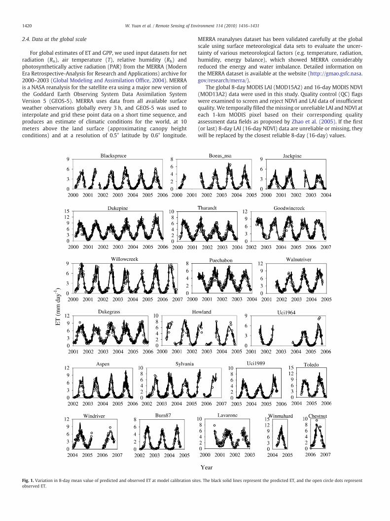
For global estimates of ET and GPP, we used input datasets for netradiation (Rn), air temperature (T), relative humidity (Rh) andphotosynthetically active radiation (PAR) from the MERRA (ModernEra Retrospective-Analysis for Research and Applications) archive for2000–2003 (Global Modeling and Assimilation Office, 2004). MERRAis a NASA reanalysis for the satellite era using a major new version ofthe Goddard Earth Observing System Data Assimilation SystemVersion 5 (GEOS-5). MERRA uses data from all available surfaceweather observations globally every 3 h, and GEOS-5 was used tointerpolate and grid these point data on a short time sequence, andproduces an estimate of climatic conditions for the world, at 10meters above the land surface (approximating canopy heightconditions) and at a resolution of 0.5° latitude by 0.6° longitude.

Fig. 1. Variation in 8-day mean value of predicted and observed ET at model calibration sitobserved ET.

MERRA reanalyses dataset has been validated carefully at the globalscale using surface meteorological data sets to evaluate the uncer-tainty of various meteorological factors (e.g. temperature, radiation,humidity, energy balance), which showed MERRA considerablyreduced the energy and water imbalance. Detailed information onthe MERRA dataset is available at the website (http://gmao.gsfc.nasa.gov/research/merra/).

The global 8-day MODIS LAI (MOD15A2) and 16-day MODIS NDVI(MOD13A2) data were used in this study. Quality control (QC) flagswere examined to screen and reject NDVI and LAI data of insufficientquality.We temporally filled themissing or unreliable LAI and NDVI ateach 1-km MODIS pixel based on their corresponding qualityassessment data fields as proposed by Zhao et al. (2005). If the first(or last) 8-day LAI (16-day NDVI) data are unreliable or missing, theywill be replaced by the closest reliable 8-day (16-day) values.

es. The black solid lines represent the predicted ET, and the open circle dots represent

1421W. Yuan et al. / Remote Sensing of Environment 114 (2010) 1416–1431

2.5. Nonlinear optimization and statistical analysis

The nonlinear regression procedure (Proc NLIN) in the StatisticalAnalysis System (SAS, SAS Institute Inc., Cary, NC, USA) was applied totwo calculations: (1) to determine the parameter values in the

Fig. 2.Variation in8-daymeanvalueofpredictedETandobservedETatmodel validationsites. Th

equation filling NEE data gaps and calculating daytime ecosystemrespiration (i.e., Eqs. (10) and (11)), and (2) to optimize the values forVPDclose, Rtot and Cl in the revised RS-PM model (see Mu et al., 2007),and Topt and εmax (see Yuan et al., 2007) in the EC-LUEmodel across allthe calibration sites.

eblacksolid lines represent thepredictedET, andtheopencircle dots representobservedET.

1422 W. Yuan et al. / Remote Sensing of Environment 114 (2010) 1416–1431

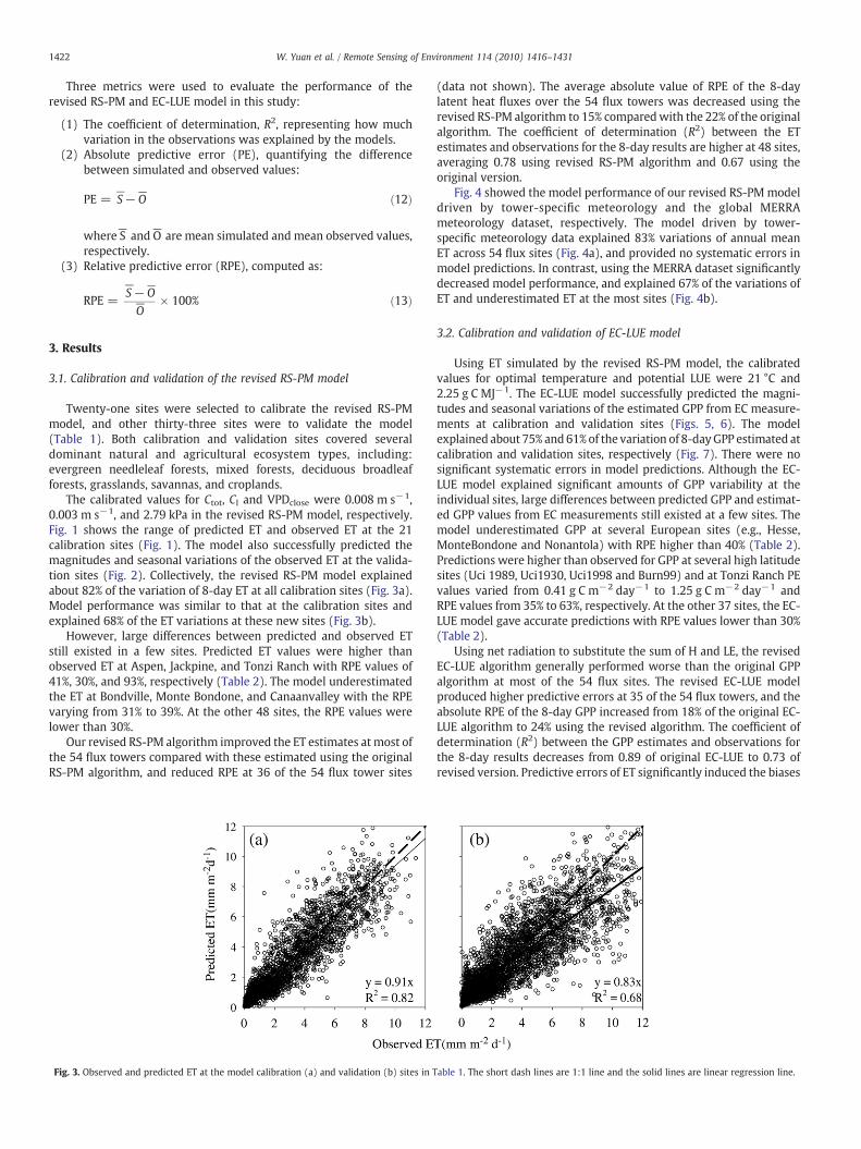
Three metrics were used to evaluate the performance of therevised RS-PM and EC-LUE model in this study:

(1) The coefficient of determination, R2, representing how muchvariation in the observations was explained by the models.

(2) Absolute predictive error (PE), quantifying the differencebetween simulated and observed values:

PE =PS−P

O ð12Þ

where S−

and O−

are mean simulated and mean observed values,respectively.

(3) Relative predictive error (RPE), computed as:

RPE =PS−P

OPO

× 100% ð13Þ

3. Results

3.1. Calibration and validation of the revised RS-PM model

Twenty-one sites were selected to calibrate the revised RS-PMmodel, and other thirty-three sites were to validate the model(Table 1). Both calibration and validation sites covered severaldominant natural and agricultural ecosystem types, including:evergreen needleleaf forests, mixed forests, deciduous broadleafforests, grasslands, savannas, and croplands.

The calibrated values for Ctot, Cl and VPDclose were 0.008 m s−1,0.003 m s−1, and 2.79 kPa in the revised RS-PM model, respectively.Fig. 1 shows the range of predicted ET and observed ET at the 21calibration sites (Fig. 1). The model also successfully predicted themagnitudes and seasonal variations of the observed ET at the valida-tion sites (Fig. 2). Collectively, the revised RS-PM model explainedabout 82% of the variation of 8-day ET at all calibration sites (Fig. 3a).Model performance was similar to that at the calibration sites andexplained 68% of the ET variations at these new sites (Fig. 3b).

However, large differences between predicted and observed ETstill existed in a few sites. Predicted ET values were higher thanobserved ET at Aspen, Jackpine, and Tonzi Ranch with RPE values of41%, 30%, and 93%, respectively (Table 2). The model underestimatedthe ET at Bondville, Monte Bondone, and Canaanvalley with the RPEvarying from 31% to 39%. At the other 48 sites, the RPE values werelower than 30%.

Our revised RS-PM algorithm improved the ET estimates at most ofthe 54 flux towers compared with these estimated using the originalRS-PM algorithm, and reduced RPE at 36 of the 54 flux tower sites

Fig. 3. Observed and predicted ET at the model calibration (a) and validation (b) sites in T

(data not shown). The average absolute value of RPE of the 8-daylatent heat fluxes over the 54 flux towers was decreased using therevised RS-PM algorithm to 15% comparedwith the 22% of the originalalgorithm. The coefficient of determination (R2) between the ETestimates and observations for the 8-day results are higher at 48 sites,averaging 0.78 using revised RS-PM algorithm and 0.67 using theoriginal version.

Fig. 4 showed the model performance of our revised RS-PMmodeldriven by tower-specific meteorology and the global MERRAmeteorology dataset, respectively. The model driven by tower-specific meteorology data explained 83% variations of annual meanET across 54 flux sites (Fig. 4a), and provided no systematic errors inmodel predictions. In contrast, using the MERRA dataset significantlydecreased model performance, and explained 67% of the variations ofET and underestimated ET at the most sites (Fig. 4b).

3.2. Calibration and validation of EC-LUE model

Using ET simulated by the revised RS-PM model, the calibratedvalues for optimal temperature and potential LUE were 21 °C and2.25 g C MJ−1. The EC-LUE model successfully predicted the magni-tudes and seasonal variations of the estimated GPP from EC measure-ments at calibration and validation sites (Figs. 5, 6). The modelexplained about 75% and61% of the variation of 8-dayGPP estimated atcalibration and validation sites, respectively (Fig. 7). There were nosignificant systematic errors in model predictions. Although the EC-LUE model explained significant amounts of GPP variability at theindividual sites, large differences between predicted GPP and estimat-ed GPP values from EC measurements still existed at a few sites. Themodel underestimated GPP at several European sites (e.g., Hesse,MonteBondone and Nonantola) with RPE higher than 40% (Table 2).Predictions were higher than observed for GPP at several high latitudesites (Uci 1989, Uci1930, Uci1998 and Burn99) and at Tonzi Ranch PEvalues varied from 0.41 g C m−2 day−1 to 1.25 g C m−2 day−1 andRPE values from 35% to 63%, respectively. At the other 37 sites, the EC-LUE model gave accurate predictions with RPE values lower than 30%(Table 2).

Using net radiation to substitute the sum of H and LE, the revisedEC-LUE algorithm generally performed worse than the original GPPalgorithm at most of the 54 flux sites. The revised EC-LUE modelproduced higher predictive errors at 35 of the 54 flux towers, and theabsolute RPE of the 8-day GPP increased from 18% of the original EC-LUE algorithm to 24% using the revised algorithm. The coefficient ofdetermination (R2) between the GPP estimates and observations forthe 8-day results decreases from 0.89 of original EC-LUE to 0.73 ofrevised version. Predictive errors of ET significantly induced the biases

able 1. The short dash lines are 1:1 line and the solid lines are linear regression line.

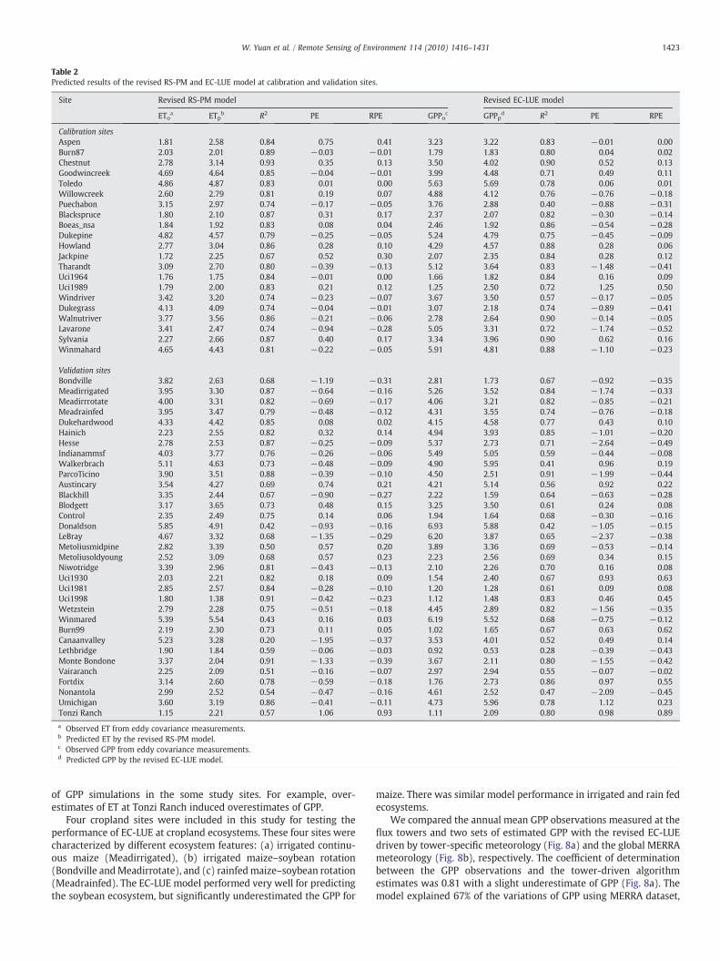
Table 2Predicted results of the revised RS-PM and EC-LUE model at calibration and validation sites.

Site Revised RS-PM model Revised EC-LUE model

EToa ETpb R2 PE RPE GPPoc GPPpd R2 PE RPE

Calibration sitesAspen 1.81 2.58 0.84 0.75 0.41 3.23 3.22 0.83 −0.01 0.00Burn87 2.03 2.01 0.89 −0.03 −0.01 1.79 1.83 0.80 0.04 0.02Chestnut 2.78 3.14 0.93 0.35 0.13 3.50 4.02 0.90 0.52 0.13Goodwincreek 4.69 4.64 0.85 −0.04 −0.01 3.99 4.48 0.71 0.49 0.11Toledo 4.86 4.87 0.83 0.01 0.00 5.63 5.69 0.78 0.06 0.01Willowcreek 2.60 2.79 0.81 0.19 0.07 4.88 4.12 0.76 −0.76 −0.18Puechabon 3.15 2.97 0.74 −0.17 −0.05 3.76 2.88 0.40 −0.88 −0.31Blackspruce 1.80 2.10 0.87 0.31 0.17 2.37 2.07 0.82 −0.30 −0.14Boeas_nsa 1.84 1.92 0.83 0.08 0.04 2.46 1.92 0.86 −0.54 −0.28Dukepine 4.82 4.57 0.79 −0.25 −0.05 5.24 4.79 0.75 −0.45 −0.09Howland 2.77 3.04 0.86 0.28 0.10 4.29 4.57 0.88 0.28 0.06Jackpine 1.72 2.25 0.67 0.52 0.30 2.07 2.35 0.84 0.28 0.12Tharandt 3.09 2.70 0.80 −0.39 −0.13 5.12 3.64 0.83 −1.48 −0.41Uci1964 1.76 1.75 0.84 −0.01 0.00 1.66 1.82 0.84 0.16 0.09Uci1989 1.79 2.00 0.83 0.21 0.12 1.25 2.50 0.72 1.25 0.50Windriver 3.42 3.20 0.74 −0.23 −0.07 3.67 3.50 0.57 −0.17 −0.05Dukegrass 4.13 4.09 0.74 −0.04 −0.01 3.07 2.18 0.74 −0.89 −0.41Walnutriver 3.77 3.56 0.86 −0.21 −0.06 2.78 2.64 0.90 −0.14 −0.05Lavarone 3.41 2.47 0.74 −0.94 −0.28 5.05 3.31 0.72 −1.74 −0.52Sylvania 2.27 2.66 0.87 0.40 0.17 3.34 3.96 0.90 0.62 0.16Winmahard 4.65 4.43 0.81 −0.22 −0.05 5.91 4.81 0.88 −1.10 −0.23

Validation sitesBondville 3.82 2.63 0.68 −1.19 −0.31 2.81 1.73 0.67 −0.92 −0.35Meadirrigated 3.95 3.30 0.87 −0.64 −0.16 5.26 3.52 0.84 −1.74 −0.33Meadirrrotate 4.00 3.31 0.82 −0.69 −0.17 4.06 3.21 0.82 −0.85 −0.21Meadrainfed 3.95 3.47 0.79 −0.48 −0.12 4.31 3.55 0.74 −0.76 −0.18Dukehardwood 4.33 4.42 0.85 0.08 0.02 4.15 4.58 0.77 0.43 0.10Hainich 2.23 2.55 0.82 0.32 0.14 4.94 3.93 0.85 −1.01 −0.20Hesse 2.78 2.53 0.87 −0.25 −0.09 5.37 2.73 0.71 −2.64 −0.49Indianammsf 4.03 3.77 0.76 −0.26 −0.06 5.49 5.05 0.59 −0.44 −0.08Walkerbrach 5.11 4.63 0.73 −0.48 −0.09 4.90 5.95 0.41 0.96 0.19ParcoTicino 3.90 3.51 0.88 −0.39 −0.10 4.50 2.51 0.91 −1.99 −0.44Austincary 3.54 4.27 0.69 0.74 0.21 4.21 5.14 0.56 0.92 0.22Blackhill 3.35 2.44 0.67 −0.90 −0.27 2.22 1.59 0.64 −0.63 −0.28Blodgett 3.17 3.65 0.73 0.48 0.15 3.25 3.50 0.61 0.24 0.08Control 2.35 2.49 0.75 0.14 0.06 1.94 1.64 0.68 −0.30 −0.16Donaldson 5.85 4.91 0.42 −0.93 −0.16 6.93 5.88 0.42 −1.05 −0.15LeBray 4.67 3.32 0.68 −1.35 −0.29 6.20 3.87 0.65 −2.37 −0.38Metoliusmidpine 2.82 3.39 0.50 0.57 0.20 3.89 3.36 0.69 −0.53 −0.14Metoliusoldyoung 2.52 3.09 0.68 0.57 0.23 2.23 2.56 0.69 0.34 0.15Niwotridge 3.39 2.96 0.81 −0.43 −0.13 2.10 2.26 0.70 0.16 0.08Uci1930 2.03 2.21 0.82 0.18 0.09 1.54 2.40 0.67 0.93 0.63Uci1981 2.85 2.57 0.84 −0.28 −0.10 1.20 1.28 0.61 0.09 0.08Uci1998 1.80 1.38 0.91 −0.42 −0.23 1.12 1.48 0.83 0.46 0.45Wetzstein 2.79 2.28 0.75 −0.51 −0.18 4.45 2.89 0.82 −1.56 −0.35Winmared 5.39 5.54 0.43 0.16 0.03 6.19 5.52 0.68 −0.75 −0.12Burn99 2.19 2.30 0.73 0.11 0.05 1.02 1.65 0.67 0.63 0.62Canaanvalley 5.23 3.28 0.20 −1.95 −0.37 3.53 4.01 0.52 0.49 0.14Lethbridge 1.90 1.84 0.59 −0.06 −0.03 0.92 0.53 0.28 −0.39 −0.43Monte Bondone 3.37 2.04 0.91 −1.33 −0.39 3.67 2.11 0.80 −1.55 −0.42Vairaranch 2.25 2.09 0.51 −0.16 −0.07 2.97 2.94 0.55 −0.07 −0.02Fortdix 3.14 2.60 0.78 −0.59 −0.18 1.76 2.73 0.86 0.97 0.55Nonantola 2.99 2.52 0.54 −0.47 −0.16 4.61 2.52 0.47 −2.09 −0.45Umichigan 3.60 3.19 0.86 −0.41 −0.11 4.73 5.96 0.78 1.12 0.23Tonzi Ranch 1.15 2.21 0.57 1.06 0.93 1.11 2.09 0.80 0.98 0.89

a Observed ET from eddy covariance measurements.b Predicted ET by the revised RS-PM model.c Observed GPP from eddy covariance measurements.d Predicted GPP by the revised EC-LUE model.

1423W. Yuan et al. / Remote Sensing of Environment 114 (2010) 1416–1431

of GPP simulations in the some study sites. For example, over-estimates of ET at Tonzi Ranch induced overestimates of GPP.

Four cropland sites were included in this study for testing theperformance of EC-LUE at cropland ecosystems. These four sites werecharacterized by different ecosystem features: (a) irrigated continu-ous maize (Meadirrigated), (b) irrigated maize–soybean rotation(Bondville andMeadirrotate), and (c) rainfedmaize–soybean rotation(Meadrainfed). The EC-LUE model performed very well for predictingthe soybean ecosystem, but significantly underestimated the GPP for

maize. There was similar model performance in irrigated and rain fedecosystems.

We compared the annual mean GPP observations measured at theflux towers and two sets of estimated GPP with the revised EC-LUEdriven by tower-specific meteorology (Fig. 8a) and the global MERRAmeteorology (Fig. 8b), respectively. The coefficient of determinationbetween the GPP observations and the tower-driven algorithmestimates was 0.81 with a slight underestimate of GPP (Fig. 8a). Themodel explained 67% of the variations of GPP using MERRA dataset,

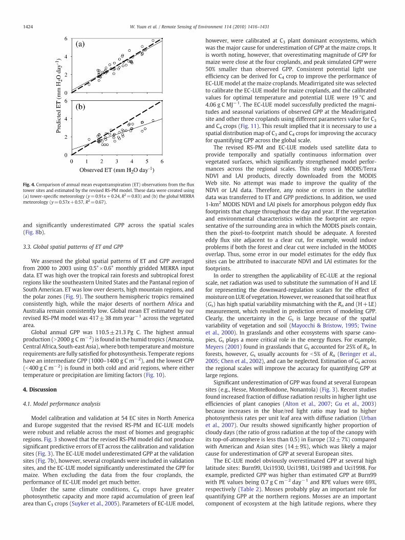
Fig. 4. Comparison of annual mean evapotranspiration (ET) observations from the fluxtower sites and estimated by the revised RS-PM model. These data were created using(a) tower-specific meteorology (y=0.91x+0.24, R2=0.83) and (b) the global MERRAmeteorology (y=0.57x+0.57, R2=0.67).

1424 W. Yuan et al. / Remote Sensing of Environment 114 (2010) 1416–1431

and significantly underestimated GPP across the spatial scales(Fig. 8b).

3.3. Global spatial patterns of ET and GPP

We assessed the global spatial patterns of ET and GPP averagedfrom 2000 to 2003 using 0.5°×0.6° monthly gridded MERRA inputdata. ET was high over the tropical rain forests and subtropical forestregions like the southeastern United States and the Pantanal region ofSouth American. ET was low over deserts, high mountain regions, andthe polar zones (Fig. 9). The southern hemispheric tropics remainedconsistently high, while the major deserts of northern Africa andAustralia remain consistently low. Global mean ET estimated by ourrevised RS-PM model was 417±38 mm year−1 across the vegetatedarea.

Global annual GPP was 110.5±21.3 Pg C. The highest annualproduction (N2000 g C m−2) is found in the humid tropics (Amazonia,Central Africa, South-east Asia),where both temperature andmoisturerequirements are fully satisfied for photosynthesis. Temperate regionshave an intermediate GPP (1000–1400 g C m−2), and the lowest GPP(b400 g C m−2) is found in both cold and arid regions, where eithertemperature or precipitation are limiting factors (Fig. 10).

4. Discussion

4.1. Model performance analysis

Model calibration and validation at 54 EC sites in North Americaand Europe suggested that the revised RS-PM and EC-LUE modelswere robust and reliable across the most of biomes and geographicregions. Fig. 3 showed that the revised RS-PM model did not producesignificant predictive errors of ET across the calibration and validationsites (Fig. 3). The EC-LUE model underestimated GPP at the validationsites (Fig. 7b), however, several croplands were included in validationsites, and the EC-LUE model significantly underestimated the GPP formaize. When excluding the data from the four croplands, theperformance of EC-LUE model get much better.

Under the same climate conditions, C4 crops have greaterphotosynthetic capacity and more rapid accumulation of green leafarea than C3 crops (Suyker et al., 2005). Parameters of EC-LUE model,

however, were calibrated at C3 plant dominant ecosystems, whichwas the major cause for underestimation of GPP at the maize crops. Itis worth noting, however, that overestimating magnitude of GPP formaize were close at the four croplands, and peak simulated GPP were50% smaller than observed GPP. Consistent potential light useefficiency can be derived for C4 crop to improve the performance ofEC-LUEmodel at the maize croplands. Meadirrigated site was selectedto calibrate the EC-LUE model for maize croplands, and the calibratedvalues for optimal temperature and potential LUE were 19 °C and4.06 g C MJ−1. The EC-LUE model successfully predicted the magni-tudes and seasonal variations of observed GPP at the Meadirrigatedsite and other three croplands using different parameters value for C3

and C4 crops (Fig. 11). This result implied that it is necessary to use aspatial distribution map of C3 and C4 crops for improving the accuracyfor quantifying GPP across the global scale.

The revised RS-PM and EC-LUE models used satellite data toprovide temporally and spatially continuous information overvegetated surfaces, which significantly strengthened model perfor-mances across the regional scales. This study used MODIS/TerraNDVI and LAI products, directly downloaded from the MODISWeb site. No attempt was made to improve the quality of theNDVI or LAI data. Therefore, any noise or errors in the satellitedata was transferred to ET and GPP predictions. In addition, we used1-km2 MODIS NDVI and LAI pixels for amorphous polygon eddy fluxfootprints that change throughout the day and year. If the vegetationand environmental characteristics within the footprint are repre-sentative of the surrounding area in which the MODIS pixels contain,then the pixel-to-footprint match should be adequate. A forestededdy flux site adjacent to a clear cut, for example, would induceproblems if both the forest and clear cut were included in the MODISoverlap. Thus, some error in our model estimates for the eddy fluxsites can be attributed to inaccurate NDVI and LAI estimates for thefootprints.

In order to strengthen the applicability of EC-LUE at the regionalscale, net radiation was used to substitute the summation of H and LEfor representing the downward-regulation scalars for the effect ofmoistureonLUEof vegetation. However,we reasoned that soil heatflux(Gs) has high spatial variability mismatching with the Rn and (H+LE)measurement, which resulted in prediction errors of modeling GPP.Clearly, the uncertainty in the Gs is large because of the spatialvariability of vegetation and soil (Mayocchi & Bristow, 1995; Twineet al., 2000). In grasslands and other ecosystems with sparse cano-pies, Gs plays a more critical role in the energy fluxes. For example,Meyers (2001) found in grasslands that Gs accounted for 25% of Rn. Inforests, however, Gs usually accounts for b5% of Rn (Beringer et al.,2005; Chen et al., 2002), and can be neglected. Estimation of Gs acrossthe regional scales will improve the accuracy for quantifying GPP atlarge regions.

Significant underestimation of GPP was found at several Europeansites (e.g., Hesse, MonteBondone, Nonantola) (Fig. 3). Recent studiesfound increased fraction of diffuse radiation results in higher light useefficiencies of plant canopies (Alton et al., 2007; Gu et al., 2003)because increases in the blue/red light ratio may lead to higherphotosynthesis rates per unit leaf area with diffuse radiation (Urbanet al., 2007). Our results showed significantly higher proportion ofcloudy days (the ratio of gross radiation at the top of the canopy withits top-of-atmosphere is less than 0.5) in Europe (32±7%) comparedwith American and Asian sites (14±9%), which was likely a majorcause for underestimation of GPP at several European sites.

The EC-LUE model obviously overestimated GPP at several highlatitude sites: Burn99, Uci1930, Uci1981, Uci1989 and Uci1998. Forexample, predicted GPP was higher than estimated GPP at Burn99with PE values being 0.7 g C m−2 day−1 and RPE values were 69%,respectively (Table 2). Mosses probably play an important role forquantifying GPP at the northern regions. Mosses are an importantcomponent of ecosystem at the high latitude regions, where they

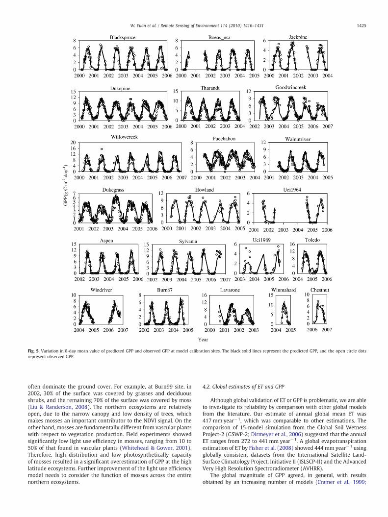
Fig. 5. Variation in 8-day mean value of predicted GPP and observed GPP at model calibration sites. The black solid lines represent the predicted GPP, and the open circle dotsrepresent observed GPP.

1425W. Yuan et al. / Remote Sensing of Environment 114 (2010) 1416–1431

often dominate the ground cover. For example, at Burn99 site, in2002, 30% of the surface was covered by grasses and deciduousshrubs, and the remaining 70% of the surface was covered by moss(Liu & Randerson, 2008). The northern ecosystems are relativelyopen, due to the narrow canopy and low density of trees, whichmakes mosses an important contributor to the NDVI signal. On theother hand, mosses are fundamentally different from vascular plantswith respect to vegetation production. Field experiments showedsignificantly low light use efficiency in mosses, ranging from 10 to50% of that found in vascular plants (Whitehead & Gower, 2001).Therefore, high distribution and low photosynthetically capacityof mosses resulted in a significant overestimation of GPP at the highlatitude ecosystems. Further improvement of the light use efficiencymodel needs to consider the function of mosses across the entirenorthern ecosystems.

4.2. Global estimates of ET and GPP

Although global validation of ET or GPP is problematic, we are ableto investigate its reliability by comparison with other global modelsfrom the literature. Our estimate of annual global mean ET was417 mm year−1, which was comparable to other estimations. Thecomparison of 15-model simulation from the Global Soil WetnessProject-2 (GSWP-2; Dirmeyer et al., 2006) suggested that the annualET ranges from 272 to 441 mm year−1. A global evapotranspirationestimation of ET by Fisher et al. (2008) showed 444 mm year−1 usingglobally consistent datasets from the International Satellite Land-Surface Climatology Project, Initiative II (ISLSCP-II) and the AdvancedVery High Resolution Spectroradiometer (AVHRR).

The global magnitude of GPP agreed, in general, with resultsobtained by an increasing number of models (Cramer et al., 1999;

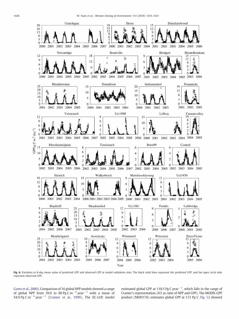
Fig. 6. Variation in 8-day mean value of predicted GPP and observed GPP at model validation sites. The black solid lines represent the predicted GPP, and the open circle dotsrepresent observed GPP.

1426 W. Yuan et al. / Remote Sensing of Environment 114 (2010) 1416–1431

Goetz et al., 2000). Comparison of 16 global NPPmodels showed a rangeof global NPP from 39.9 to 80 Pg C m−2 year−1 with a mean of54.9 Pg C m−2 year−1 (Cramer et al., 1999). The EC-LUE model

estimated global GPP at 110.5 Pg C year−1, which falls in the range ofCramer's representation (0.5 as ratio of NPP and GPP). The MODIS-GPPproduct (MOD17A) estimates global GPP at 113 Pg C. Fig. 12 showed

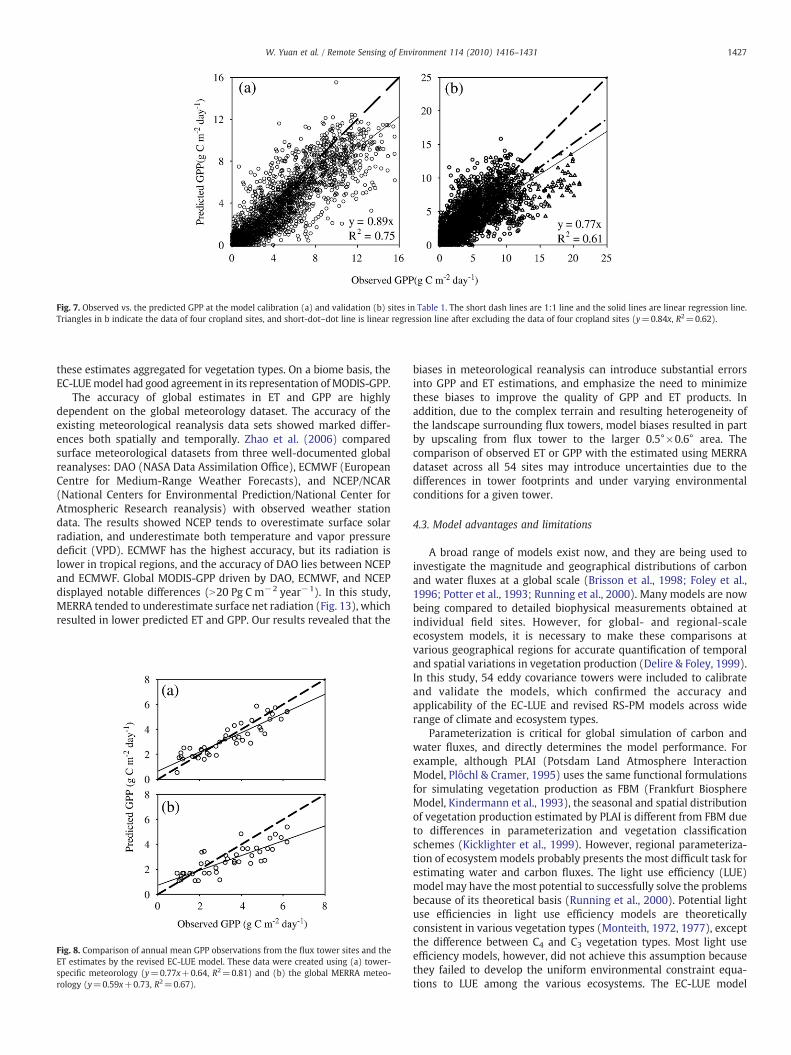
Fig. 7. Observed vs. the predicted GPP at the model calibration (a) and validation (b) sites in Table 1. The short dash lines are 1:1 line and the solid lines are linear regression line.Triangles in b indicate the data of four cropland sites, and short-dot–dot line is linear regression line after excluding the data of four cropland sites (y=0.84x, R2=0.62).

1427W. Yuan et al. / Remote Sensing of Environment 114 (2010) 1416–1431

these estimates aggregated for vegetation types. On a biome basis, theEC-LUEmodel had good agreement in its representation of MODIS-GPP.

The accuracy of global estimates in ET and GPP are highlydependent on the global meteorology dataset. The accuracy of theexisting meteorological reanalysis data sets showed marked differ-ences both spatially and temporally. Zhao et al. (2006) comparedsurface meteorological datasets from three well-documented globalreanalyses: DAO (NASA Data Assimilation Office), ECMWF (EuropeanCentre for Medium-Range Weather Forecasts), and NCEP/NCAR(National Centers for Environmental Prediction/National Center forAtmospheric Research reanalysis) with observed weather stationdata. The results showed NCEP tends to overestimate surface solarradiation, and underestimate both temperature and vapor pressuredeficit (VPD). ECMWF has the highest accuracy, but its radiation islower in tropical regions, and the accuracy of DAO lies between NCEPand ECMWF. Global MODIS-GPP driven by DAO, ECMWF, and NCEPdisplayed notable differences (N20 Pg C m−2 year−1). In this study,MERRA tended to underestimate surface net radiation (Fig. 13), whichresulted in lower predicted ET and GPP. Our results revealed that the

Fig. 8. Comparison of annual mean GPP observations from the flux tower sites and theET estimates by the revised EC-LUE model. These data were created using (a) tower-specific meteorology (y=0.77x+0.64, R2=0.81) and (b) the global MERRA meteo-rology (y=0.59x+0.73, R2=0.67).

biases in meteorological reanalysis can introduce substantial errorsinto GPP and ET estimations, and emphasize the need to minimizethese biases to improve the quality of GPP and ET products. Inaddition, due to the complex terrain and resulting heterogeneity ofthe landscape surrounding flux towers, model biases resulted in partby upscaling from flux tower to the larger 0.5°×0.6° area. Thecomparison of observed ET or GPP with the estimated using MERRAdataset across all 54 sites may introduce uncertainties due to thedifferences in tower footprints and under varying environmentalconditions for a given tower.

4.3. Model advantages and limitations

A broad range of models exist now, and they are being used toinvestigate the magnitude and geographical distributions of carbonand water fluxes at a global scale (Brisson et al., 1998; Foley et al.,1996; Potter et al., 1993; Running et al., 2000). Many models are nowbeing compared to detailed biophysical measurements obtained atindividual field sites. However, for global- and regional-scaleecosystem models, it is necessary to make these comparisons atvarious geographical regions for accurate quantification of temporaland spatial variations in vegetation production (Delire & Foley, 1999).In this study, 54 eddy covariance towers were included to calibrateand validate the models, which confirmed the accuracy andapplicability of the EC-LUE and revised RS-PM models across widerange of climate and ecosystem types.

Parameterization is critical for global simulation of carbon andwater fluxes, and directly determines the model performance. Forexample, although PLAI (Potsdam Land Atmosphere InteractionModel, Plőchl & Cramer, 1995) uses the same functional formulationsfor simulating vegetation production as FBM (Frankfurt BiosphereModel, Kindermann et al., 1993), the seasonal and spatial distributionof vegetation production estimated by PLAI is different from FBM dueto differences in parameterization and vegetation classificationschemes (Kicklighter et al., 1999). However, regional parameteriza-tion of ecosystemmodels probably presents the most difficult task forestimating water and carbon fluxes. The light use efficiency (LUE)model may have the most potential to successfully solve the problemsbecause of its theoretical basis (Running et al., 2000). Potential lightuse efficiencies in light use efficiency models are theoreticallyconsistent in various vegetation types (Monteith, 1972, 1977), exceptthe difference between C4 and C3 vegetation types. Most light useefficiency models, however, did not achieve this assumption becausethey failed to develop the uniform environmental constraint equa-tions to LUE among the various ecosystems. The EC-LUE model

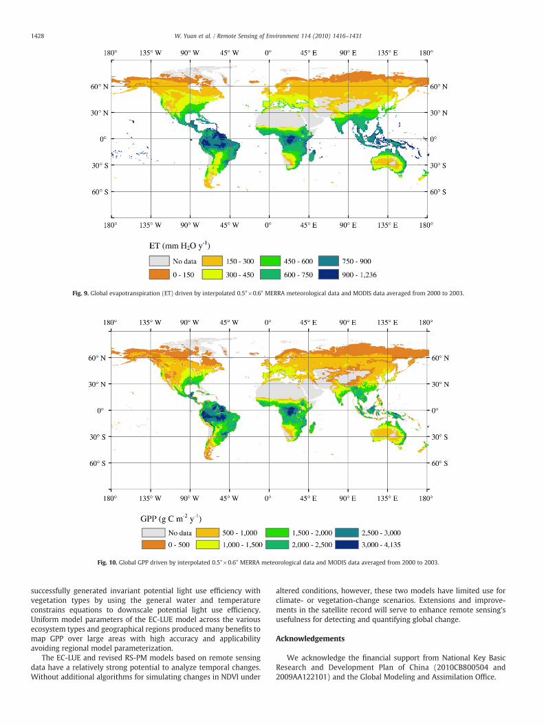
Fig. 9. Global evapotranspiration (ET) driven by interpolated 0.5°×0.6° MERRA meteorological data and MODIS data averaged from 2000 to 2003.

Fig. 10. Global GPP driven by interpolated 0.5°×0.6° MERRA meteorological data and MODIS data averaged from 2000 to 2003.

1428 W. Yuan et al. / Remote Sensing of Environment 114 (2010) 1416–1431

successfully generated invariant potential light use efficiency withvegetation types by using the general water and temperatureconstrains equations to downscale potential light use efficiency.Uniform model parameters of the EC-LUE model across the variousecosystem types and geographical regions produced many benefits tomap GPP over large areas with high accuracy and applicabilityavoiding regional model parameterization.

The EC-LUE and revised RS-PM models based on remote sensingdata have a relatively strong potential to analyze temporal changes.Without additional algorithms for simulating changes in NDVI under

altered conditions, however, these two models have limited use forclimate- or vegetation-change scenarios. Extensions and improve-ments in the satellite record will serve to enhance remote sensing'susefulness for detecting and quantifying global change.

Acknowledgements

We acknowledge the financial support from National Key BasicResearch and Development Plan of China (2010CB800504 and2009AA122101) and the Global Modeling and Assimilation Office.

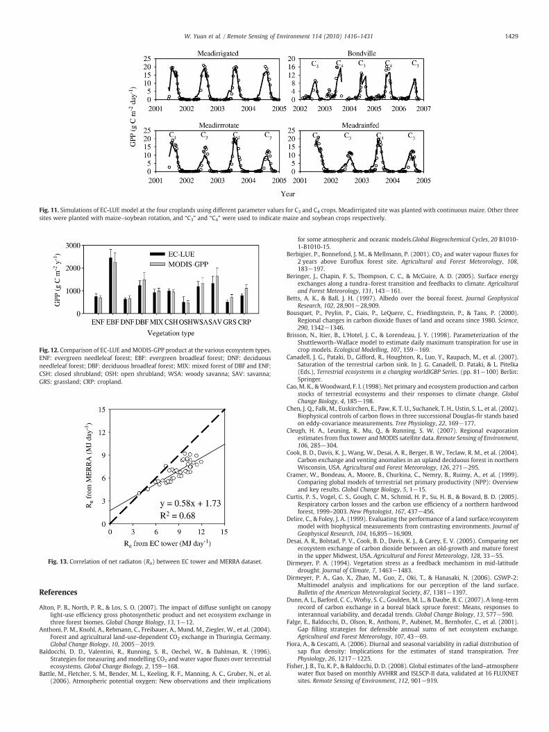
Fig. 11. Simulations of EC-LUE model at the four croplands using different parameter values for C3 and C4 crops. Meadirrigated site was planted with continuous maize. Other threesites were planted with maize–soybean rotation, and “C3” and “C4” were used to indicate maize and soybean crops respectively.

Fig. 12. Comparison of EC-LUE and MODIS-GPP product at the various ecosystem types.ENF: evergreen needleleaf forest; EBF: evergreen broadleaf forest; DNF: deciduousneedleleaf forest; DBF: deciduous broadleaf forest; MIX: mixed forest of DBF and ENF;CSH: closed shrubland; OSH: open shrubland; WSA: woody savanna; SAV: savanna;GRS: grassland; CRP: cropland.

Fig. 13. Correlation of net radiaton (Rn) between EC tower and MERRA dataset.

1429W. Yuan et al. / Remote Sensing of Environment 114 (2010) 1416–1431

References

Alton, P. B., North, P. R., & Los, S. O. (2007). The impact of diffuse sunlight on canopylight-use efficiency gross photosynthetic product and net ecosystem exchange inthree forest biomes. Global Change Biology, 13, 1−12.

Anthoni, P. M., Knohl, A., Rebmann, C., Freibauer, A., Mund, M., Ziegler, W., et al. (2004).Forest and agricultural land-use-dependent CO2 exchange in Thuringia, Germany.Global Change Biology, 10, 2005−2019.

Baldocchi, D. D., Valentini, R., Running, S. R., Oechel, W., & Dahlman, R. (1996).Strategies for measuring and modelling CO2 and water vapor fluxes over terrestrialecosystems. Global Change Biology, 2, 159−168.

Battle, M., Fletcher, S. M., Bender, M. L., Keeling, R. F., Manning, A. C., Gruber, N., et al.(2006). Atmospheric potential oxygen: New observations and their implications

for some atmospheric and oceanic models.Global Biogeochemical Cycles, 20 B1010-1-B1010-15.

Berbigier, P., Bonnefond, J. M., & Mellmann, P. (2001). CO2 and water vapour fluxes for2 years above Euroflux forest site. Agricultural and Forest Meteorology, 108,183−197.

Beringer, J., Chapin, F. S., Thompson, C. C., & McGuire, A. D. (2005). Surface energyexchanges along a tundra–forest transition and feedbacks to climate. Agriculturaland Forest Meteorology, 131, 143−161.

Betts, A. K., & Ball, J. H. (1997). Albedo over the boreal forest. Journal GeophysicalResearch, 102, 28,901−28,909.

Bousquet, P., Peylin, P., Ciais, P., LeQuere, C., Friedlingstein, P., & Tans, P. (2000).Regional changes in carbon dioxide fluxes of land and oceans since 1980. Science,290, 1342−1346.

Brisson, N., Itier, B., L'Hotel, J. C., & Lorendeau, J. Y. (1998). Parameterization of theShuttleworth–Wallace model to estimate daily maximum transpiration for use incrop models. Ecological Modelling, 107, 159−169.

Canadell, J. G., Pataki, D., Gifford, R., Houghton, R., Luo, Y., Raupach, M., et al. (2007).Saturation of the terrestrial carbon sink. In J. G. Canadell, D. Pataki, & L. Pitelka(Eds.), Terrestrial ecosystems in a changing worldIGBP Series. (pp. 81−100) Berlin:Springer.

Cao, M. K., &Woodward, F. I. (1998). Net primary and ecosystem production and carbonstocks of terrestrial ecosystems and their responses to climate change. GlobalChange Biology, 4, 185−198.

Chen, J. Q., Falk, M., Euskirchen, E., Paw, K. T. U., Suchanek, T. H., Ustin, S. L., et al. (2002).Biophysical controls of carbon flows in three successional Douglas-fir stands basedon eddy-covariance measurements. Tree Physiology, 22, 169−177.

Cleugh, H. A., Leuning, R., Mu, Q., & Running, S. W. (2007). Regional evaporationestimates from flux tower andMODIS satellite data. Remote Sensing of Environment,106, 285−304.

Cook, B. D., Davis, K. J., Wang, W., Desai, A. R., Berger, B. W., Teclaw, R. M., et al. (2004).Carbon exchange and venting anomalies in an upland deciduous forest in northernWisconsin, USA. Agricultural and Forest Meteorology, 126, 271−295.

Cramer, W., Bondeau, A., Moore, B., Churkina, C., Nemry, B., Ruimy, A., et al. (1999).Comparing global models of terrestrial net primary productivity (NPP): Overviewand key results. Global Change Biology, 5, 1−15.

Curtis, P. S., Vogel, C. S., Gough, C. M., Schmid, H. P., Su, H. B., & Bovard, B. D. (2005).Respiratory carbon losses and the carbon use efficiency of a northern hardwoodforest, 1999–2003. New Phytologist, 167, 437−456.

Delire, C., & Foley, J. A. (1999). Evaluating the performance of a land surface/ecosystemmodel with biophysical measurements from contrasting environments. Journal ofGeophysical Research, 104, 16,895−16,909.

Desai, A. R., Bolstad, P. V., Cook, B. D., Davis, K. J., & Carey, E. V. (2005). Comparing netecosystem exchange of carbon dioxide between an old-growth and mature forestin the upper Midwest, USA. Agricultural and Forest Meteorology, 128, 33−55.

Dirmeyer, P. A. (1994). Vegetation stress as a feedback mechanism in mid-latitudedrought. Journal of Climate, 7, 1463−1483.

Dirmeyer, P. A., Gao, X., Zhao, M., Guo, Z., Oki, T., & Hanasaki, N. (2006). GSWP-2:Multimodel analysis and implications for our perception of the land surface.Bulletin of the American Meteorological Society, 87, 1381−1397.

Dunn, A. L., Barford, C. C., Wofsy, S. C., Goulden, M. L., & Daube, B. C. (2007). A long-termrecord of carbon exchange in a boreal black spruce forest: Means, responses tointerannual variability, and decadal trends. Global Change Biology, 13, 577−590.

Falge, E., Baldocchi, D., Olson, R., Anthoni, P., Aubinet, M., Bernhofer, C., et al. (2001).Gap filling strategies for defensible annual sums of net ecosystem exchange.Agricultural and Forest Meteorology, 107, 43−69.

Fiora, A., & Cescatti, A. (2006). Diurnal and seasonal variability in radial distribution ofsap flux density: Implications for the estimates of stand transpiration. TreePhysiology, 26, 1217−1225.

Fisher, J. B., Tu, K. P., & Baldocchi, D. D. (2008). Global estimates of the land–atmospherewater flux based on monthly AVHRR and ISLSCP-II data, validated at 16 FLUXNETsites. Remote Sensing of Environment, 112, 901−919.

1430 W. Yuan et al. / Remote Sensing of Environment 114 (2010) 1416–1431

Flanagan, L. B., & Johnson, B. G. (2005). Interacting effects of temperature, soil moistureand plant biomass production on ecosystem respiration in a northern temperategrassland. Agricultural and Forest Meteorology, 130, 237−253.

Foley, J. A., Prentice, I. C., Ramankutty, N., Levis, S., Pollard, D., Sitch, S., et al. (1996). Anintegrated biosphere model of land surface processes, terrestrial carbon balance,and vegetation dynamics. Global Biogeochemical Cycles, 10, 603−628.

Foroutan-Pour, K., Dutilleul, P., & Smith, D. L. (2001). Inclusion of the fractal dimensionof leafless plant structure in the Beer–Lambert Law. Agronomy Journal, 93,333−338.

Friedl, M. A. (1996). Relationships among remotely sensed data, surface energy balance,and area-averaged fluxes over partially vegetated land surfaces. Journal of AppliedMeteorology, 35, 2091−2103.

Friend, A. D., Arneth, A., Kiang, N. Y., Lomas, M., Ogee, J., Rodenbeck, C., et al. (2007).FLUXNET and modelling the global carbon cycle. Global Change Biology, 13,610−633.

Gash, J. H. C. (1987). An analytical framework for extrapolating evaporationmeasurements by remote sensing surface temperature. International Journal ofRemote Sensing, 8, 1245−1249.

Gholz, H. L., & Clark, K. L. (2002). Energy exchange across a chronosequence of slashpine forests in Florida. Agricultural and Forest Meteorology, 112, 87−102.

Gholz, H. L., Vogel, S. A., Cropper, W. P., Jr., McKelvey, K., Ewel, K. C., Teskey, R. O., et al.(1991). Dynamics of canopy structure and light interception in Pinus elliottii standsof north Florida. Ecological Monograph, 61, 33−51.

Global Modeling and Assimilation Office (2004). File specification for GEOSDAS griddedoutput version 5.3, report. Greenbelt, Md: NASA Goddard Space Flight Cent.

Goetz, S. J., Prince, S. D., Small, J., & Gleason, C. R. (2000). Interannual variability of globalterrestrial primary production: Results of a model driven with satellite observa-tions. Journal of Geophysical Research, 105, 20,077−20,091.

Goldstein, A. H., Hultman, N. E., Fracheboud, J. M., Bauer, M. R., Panek, J. A., Xu, M., et al.(2000). Effects of climate variability on the carbon dioxide, water, and sensible heatfluxes above a ponderosa pine plantation in the Sierra Nevada (CA). Agriculturaland Forest Meteorology, 101, 113−129.

Goulden, M. L., Winston, G. C., McMillan, A. M. S., Litvak, M. E., Read, E. L., Rocha, A. V.,et al. (2006). An eddy covariance mesonet to measure the effect of forest age onland–atmosphere exchange. Global Change Biology, 12, 2146−2162.

Granier, A., Ceschia, C., Damesin, C., Dufrene, E., & Epron, D. (2000). The carbon balanceof a young Beech forest. Functional Ecology, 14, 312−325.

Griffis, T. J., Black, T. A., Morgenstern, K., Barr, A. G., Nesic, Z., Drewitt, G. B., et al. (2003).Ecophysiological controls on the carbon balances of three southern boreal forests.Agricultural and Forest Meteorology, 117, 53−71.

Grünwald, T., & Berhofer, C. (2007). A decade of carbon, water and energy fluxmeasurements of an old spruce forest at the Anchor Station Tharandt. Tellus, 59B,387−396.

Gu, L. H., Baldocchi, D. D., Wofsy, S. C., Munger, J. W., Michalsky, J. J., Urbanski, S. P., et al.(2003). Response of a deciduous forest to the Mount Pinatubo Eruption: Enhancedphotosynthesis. Science, 299, 2035−2038.

Hollinger, D. Y., Aber, J., Dail, B., Davidson, E. A., Goltz, S. M., Hughes, H., et al. (2004).Spatial and temporal variability in forest–atmosphere CO2 exchange. Global ChangeBiology, 10, 1689−1706.

June, T., Evans, J. R., & Farquhar, G. D. (2004). A simple new equation for the reversibletemperature dependence of photosynthetic electron transport: A study on soybeanleaf. Functional Plant Biology, 31, 275−283.

Keane, R. E., Ryan, K. C., Veblen, T. T., Allen, C. D., Logan, J., & Hawkes, B. (2002).Cascading effects of fire exclusion in Rocky Mountain ecosystems: A literaturereview. USDA forest service gen. tech. report RMRS-GTR-91 (24 pp.).

Kicklighter, D. W., Bondeau, A., Schloss, A. L., Kaduk, J., & Mcguire, A. D.the Participantsof the Potsdam NPP model intercomparison. (1999). Comparing global models ofterrestrial net primary productivity (NPP): Global pattern and differentiation bymajor biomes. Global Change Biology, 5, 16−24.

Kindermann, J., Lüdeke, M. K. B., Badeck, F. W., Otto, R. D., Klaudius, A., Häger, C. H., et al.(1993). Structure of a global and seasonal carbon exchangemodel for the terrestrialbiosphere: The Frankfurt Biosphere Model (FBM). Water, Air and Soil Pollution, 70,675−684.

Knohl, A., Schulze, E. D., Kolle, O., & Buchmann, N. (2003). Large carbon uptake by anunmanaged 250-year-old deciduous forest in Central Germany. Agricultural andForest Meteorology, 118, 151−167.

Kustas, W. P., & Norman, J. M. (1996). Use of remote sensing for evapotranspirationmonitoring over land surfaces. Hydrological Sciences, 41, 495−516.

Landsberg, J. J. (1986). Physiological ecology of forest production (pp. 165−178). London:Academic Press.

Law, B. E., Turner, D., Campbell, J., Sun, O. J., Tuyl, S. V., Ritts, W. D., et al. (2004).Disturbance and climate effects on carbon stocks and fluxes acrossWestern OregonUSA. Global Change Biology, 10, 1429−1444.

Law, B. E., Williams, M., Anthoni, P. M., Baldocchi, D. D., & Unsworth, M. H. (2000).Measuring and modelling seasonal variation of carbon dioxide and water vapourexchange of a Pinus ponderosa forest subject to soil water deficit. Global ChangeBiology, 6, 613−630.

Lettenmaier, D. P., & Famiglietti, J. S. (2006). Water from on high. Nature, 444, 562−563.Liu, H. P., & Randerson, J. T. (2008). Interannual variability of surface energy exchange

depends on stand age in a boreal forest fire chronosequence. Journal of GeophysicalResearch, 13, G01006, doi:10.1029/2007JG000483.

Lloyd, J., & Taylor, J. A. (1994). On the temperature dependence of soil respiration.Functional Ecology, 8, 315−323.

Ma, S., Baldocchi, D. D., Xu, L., & Hehn, T. (2007). Inter-annual variability in carbondioxide exchange of an oak/grass savanna and open grassland in California.Agricultural and Forest Meteorology, 147, 157−171.

Marcolla, B., & Cescatti, A. (2005). Experimental analysis of flux footprint for varyingstability conditions in an alpine meadow. Agricultural and Forest Meteorology, 135,291−301.

Mayocchi, C. L., & Bristow, K. L. (1995). Soil surface heat flux: some general questionsand comments on measurements. Agricultural and Forest Meteorology, 75, 43−50.

McVicar, T. R., & Jupp, D. L. B. (1998). The current and potential operational uses ofremote sensing to aid decisions on drought exceptional circumstances in Australia:A review. Agricultural Systems, 57, 399−468.

Meyer, W. (1999). Standard reference evaporation calculation for inland, south easternAustralia. Technical report, 35/98,Adelaide, South Australia: CSIRO Land and Water.

Meyers, T. P. (2001). A comparison of summertime water and CO2 fluxes overrangeland for well watered and drought conditions. Agricultural and ForestMeteorology, 106, 205−214.

Meyers, T. P., & Hollinger, S. E. (2004). An assessment of storage terms in the surfaceenergy balance of maize and soybean. Agricultural and Forest Meteorology, 125,105−115.

Migliavacca, M., Meroni, M., Busetto, L., Colombo, R., Zenone, T., Matteucci, G., et al.(2009). Modeling gross primary production of agro-forestry ecosystems byassimilation of satellite derived information in a process-based model. Sensors, 9,922−942.

Monsi, M., & Saeki, T. (1953). Über den Lichtfaktor in den Pflanzengesellschaften undseine Bedeutung für die Stoffproduktion. Japanese Journal of Botany, 14, 22−52.

Monson, R. K., Sparks, J. P., Rosenstiel, T. N., Scott-Denton, L. E., Huxman, T. E., Harley, P. C.,et al. (2005). Climatic influences on net ecosystem CO2 exchange during thetransition from wintertime carbon source to springtime carbon sink in a high-elevation, subalpine forest. Oecologia, 146, 130−147.

Monteith, J. L. (1972). Solar radiation and productivity in tropical ecosystems. Journal ofApplied Ecology, 9, 747−766.

Monteith, J. L. (1977). Climate and the efficiency of crop production in Britain.Philosophical Transactions of the Royal Society of London, 281, 277−294.

Mu, Q. Z., Heinsch, F. A., Zhao, M. S., & Running, S. W. (2007). Development of a globalevapotranspiration algorithm based on MODIS and global meteorology data.Remote Sensing of Environment, 111, 519−536.

Noormets, A., Chen, J. Q., & Crow, T. R. (2007). Age-dependent changes in ecosystemcarbon fluxes in managed forests in Northern Wisconsin, USA. Ecosystems, 10,1432−9840.

Novick, K. A., Stoy, P. C., Katul, G. G., Ellsworth, D. S., Siqueira, D. S., Juang, J., et al. (2004).Carbon dioxide and water vapor exchange in a warm temperate grassland.Oecologia, 138, 259−274.

Papale, D., Reichstein, M., Aubinet, M., Canfora, E., Bernhofer, C., Kutsch, W., et al.(2006). Towards a standardized processing of Net Ecosystem Exchange measuredwith eddy covariance technique: Algorithms and uncertainty estimation. Biogeos-ciences, 3, 571−583.

Pataki, D. E., & Oren, R. (2003). Species differences in stomatal control of water loss atthe canopy scale in a mature bottomland deciduous forest. Advances in WaterResources, 26, 1267−1278.

Paw, U. K. T., Falk, M., Suchanek, T. H., Ustin, S. L., Chen, J. Q., Park, Y. S., et al. (2004).Carbon dioxide exchange between an old-growth forest and the atmosphere.Ecosystems, 7, 513−524.

Pielke, R. S., Sr., Avissar, R., Raupach, M., Dolman, A. J., Zeng, X., & Denning, A. S. (1998).Interactions between the atmosphere and terrestrial ecosystems: Influence onweather and climate. Global Change Biology, 4, 461−475.

Plőchl, M., & Cramer, W. (1995). Coupling global models of vegetation structure andecosystem processes an example from arctic and boreal ecosystems. Tellus(B), 47,240−250.

Potter, C. B., Randerson, J. T., Field, C. B., Matson, P. A., Vitousek, P. M., Mooney, H. A.,et al. (1993). Terrestrial ecosystem production: A process model based on globalsatellite and surface data. Global Biogeochemistry Cycle, 7, 811−841.

Rambal, S., Joffre, R., Ourcival, J. M., Cavender-Bares, J., & Rocheteau, A. (2004). Thegrowth respiration component in eddy CO2 flux from a Quercusilex Mediterraneanforest. Global Change Biology, 10, 1460−1469.

Raupach, M. R. (2001). Combination theory and equilibrium evaporation. QuarterlyJournal of the Royal Meteorological Society, 127, 1149−1181.

Reichstein,M., Falge, E., Baldocchi, D., Papale, D., Aubinet, M., Berbigier, P., et al. (2005). Onthe separation of net ecosystem exchange into assimilation and ecosystemrespiration: Review and improved algorithm. Global Change Biology, 11, 1424−1439.

Ruimy, A., Kergoat, L., & Bondeau, A.the Participants of the Potsdam NPP modelintercomparison. (1999). Comparing global models of terrestrial net primaryproductivity (NPP): analysis of differences in light absorption and light-useefficiency. Global Change Biology, 5, 56−64.

Running, S. W., Nemani, R. R., Heinsch, F. A., Zhao, M. S., Reeves, M., & Hashimoto, H.(2004). A continuous satellite-derived measure of global terrestrial primaryproduction. Bioscience, 54, 547−560.

Running, S. W., Thornton, P. E., Nemani, R., & Glassy, J. M. (2000). Global terrestrial grossand net primary productivity from the earth observing system. In O. E. Sala, R. B.Jackson, & H. A. Mooney (Eds.), Methods in ecosystem science (pp. 44−57). NewYork: Springer-Verlag.

Ryu, Y., Baldocchi, D. D., Ma, S., & Hehn, T. (2008). Interannual variability ofevapotranspiration and energy exchanges over an annual grassland in California.Journal ofGeophysical Research-Atmospheres,113(D09104), doi:10.1029/2007JD009263.

Schimel, D. S., House, J. I., Hibbard, K. A., Bousquet, P., Ciais, P., Peylin, P., et al. (2001).Recent patterns and mechanisms of carbon exchange by terrestrial ecosystems.Nature, 414, 169−172.

Schmid, H. P., Grimmond, C. S. B., Cropley, F., Offerle, B., & Su, H. B. (2000).Measurements of CO2 and energy fluxes over a mixed hardwood forest in themid-western United States. Agricultural and Forest Meteorology, 103, 357−374.

1431W. Yuan et al. / Remote Sensing of Environment 114 (2010) 1416–1431

Schreiber, L., Skrabs, M., Hartmann, K. D., Diamantopoulos, P., Šimáňová, E., &Šantrůček, J. (2001). Effect of humidity on cuticular water permeability of isolatedcuticular membranes and leaf disks. Planta, 214, 274−282.

Song, J., Liao, K., Coulter, R. L., & Lesht, B. M. (2005). Climatology of the low-level jet atthe southern Great Plains atmospheric Boundary Layer Experiments site. Journal ofApplied Meteorology, 44, 1593−1606.

Stoy, P. C., Katul, G. G., Siqueira, M. B. S., Juang, J. Y., Novick, K. A., Mccarthy, H. R., et al.(2008). Role of vegetation in determining carbon sequestration along ecologicalsuccession in the southeasternUnited States.Global Change Biology, 14, 1409−1427.

Suyker, A. E., Verma, S. B., Burba, G. G., & Arkebauer, T. J. (2005). Gross primaryproduction and ecosystem respiration of irrigated maize and irrigated soybeanduring a growing season. Agricultural and Forest Meteorology, 131, 180−190.

Twine, T. E., Kustas, W. P., Norman, J. M., Cook, D. R., Houser, P. R., Meyers, T. P., et al.(2000). Correcting eddy-covariance flux underestimates over a grassland.Agricultural and Forest Meteorology, 103, 279−300.

Urban, O., Janous, D., Acosta, M., Czerný, R., Markovà, I., Navràtil, M., et al. (2007).Ecophysiological controls over the net ecosystem exchange of mountain sprucestand. Comparison of the response in direct vs. diffuse solar radiation. GlobalChange Biology, 13, 157−168.

Valentini, R. (2003). Fluxes of carbon, water and energy of European forests.Heidelberg:Springer Verlag (260 pp.).

Verma, S. B., Dobermann, A., Cassman, K. G., Walters, D. T., Knops, J. M., Arkebauer, T. J.,et al. (2005). Annual carbon dioxide exchange in irrigated and rainfed maize-basedagroecosystems. Agricultural and Forest Meteorology, 131, 77−96.

Vose, J. M., Sullivan, N. H., Clinton, B. D., & Bolstad, P. V. (1995). Vertical leaf areadistribution, light transmittance, and application of the Beer–Lambert Law in fourmature hardwood stands in the southern Appalachians. Canadian Journal of ForestResearch, 25, 1036−1043.

Whitehead, D., & Gower, S. T. (2001). Photosynthesis and light-use efficiency by plantsin a Canadian boreal forest ecosystem. Tree Physiology, 21, 925−929.

Wilson, K. B., & Baldocchi, D. D. (2000). Seasonal and interannual variability of energyfluxes over a broadleaved temperate deciduous forest in North American.Agricultural and Forest Meteorology, 100, 1−18.

Yuan, W. P., Liu, S. G., Zhou, G. S., Zhou, G. Y., Tieszen, L. L., Baldocchi, D., et al. (2007).Deriving a light use efficiency model from eddy covariance flux data for predictingdaily gross primary production across biomes. Agricultural and Forest Meteorology,143, 189−207.

Zhao, M., Heinsch, F. A., Nemani, R., & Running, S. W. (2005). Improvements of theMODIS terrestrial gross and net primary production global data set. Remote Sensingof Environment, 95, 164−176.

Zhao, M., Running, S. W., & Nemani, R. R. (2006). Sensitivity of Moderate ResolutionImaging Spectroradiometer (MODIS) terrestrial primary production to theaccuracy of meteorological reanalyses. Journal of Geophysical Research, 111,G01002, doi:10.1029/2004JG000004.

Zhang, Y. C., Rossow,W. B., Lacis, A. A., Oinas, V., &Mishchenko, M. I. (2004). Calculationof radiative fluxes from the surface to top of atmosphere based on ISCCP and otherglobal data sets: Refinements of the radiative transfer model and the input data.Journal of Geophysical Research, 109, D19105, doi:10.1029/2003JD004457.