Remote Sensing of Environment 114 (2010) 504–513

Contents lists available at ScienceDirect

Remote Sensing of Environment

j ourna l homepage: www.e lsev ie r.com/ locate / rse

https://ntrs.nasa.gov/search.jsp?R=20110015410 2018-08-18T08:42:37+00:00Z

Remote sensing of the urban heat island effect across biomes in the continental USA

Marc L. Imhoff a,⁎, Ping Zhang a,b, Robert E. Wolfe a, Lahouari Bounoua a

a Hydrospheric and Biospheric Science Laboratory, NASA's Goddard Space Flight Center, Greenbelt, MD, 20771, USAb Earth Resource Technology Inc., Annapolis Junction, MD, 20701, USA

⁎ Corresponding author. Biospheric Sciences BranchSpace Flight Center, Greenbelt, MD, 20771, USA. Tel.: +614 6695.

E-mail address: Marc.L.Imhoff@nasa.gov (M.L. Imho

0034-4257/$ – see front matter. Published by Elsevierdoi:10.1016/j.rse.2009.10.008

a b s t r a c t

a r t i c l e i n f o

Article history:Received 4 August 2009Received in revised form 6 October 2009Accepted 9 October 2009

Keywords:Urban heat islandRemote sensingMODISLand surface temperatureBiomesLandsatImpervious surface area

Impervious surface area (ISA) from the Landsat TM-based NLCD 2001 dataset and land surface temperature(LST) from MODIS averaged over three annual cycles (2003–2005) are used in a spatial analysis to assess theurban heat island (UHI) skin temperature amplitude and its relationship to development intensity, size, andecological setting for 38 of the most populous cities in the continental United States. Development intensityzones based on %ISA are defined for each urban area emanating outward from the urban core to the non-urban rural areas nearby and used to stratify sampling for land surface temperatures and NDVI. Sampling isfurther constrained by biome and elevation to insure objective intercomparisons between zones andbetween cities in different biomes permitting the definition of hierarchically ordered zones that areconsistent across urban areas in different ecological setting and across scales.We find that ecological context significantly influences the amplitude of summer daytime UHI (urban–ruraltemperature difference) the largest (8 °C average) observed for cities built in biomes dominated bytemperate broadleaf and mixed forest. For all cities combined, ISA is the primary driver for increase intemperature explaining 70% of the total variance in LST. On a yearly average, urban areas are substantiallywarmer than the non-urban fringe by 2.9 °C, except for urban areas in biomes with arid and semiaridclimates. The average amplitude of the UHI is remarkably asymmetric with a 4.3 °C temperature differencein summer and only 1.3 °C in winter. In desert environments, the LST's response to ISA presents anuncharacteristic “U-shaped” horizontal gradient decreasing from the urban core to the outskirts of the cityand then increasing again in the suburban to the rural zones. UHI's calculated for these cities point to apossible heat sink effect. These observational results show that the urban heat island amplitude bothincreases with city size and is seasonally asymmetric for a large number of cities across most biomes. Theimplications are that for urban areas developed within forested ecosystems the summertime UHI can bequite high relative to the wintertime UHI suggesting that the residential energy consumption required forsummer cooling is likely to increase with urban growth within those biomes.

Code 614.4, NASA's Goddard1 301 614 6628; fax: +1 301

ff).

Inc.

Published by Elsevier Inc.

1. Introduction

In 2008 more than half of the world's population were urbandwellers and the urban population is expected to reach 81% by 2030(UNFPA, 2007). As the process of global urbanization accelerates bothin intensity and area there is growing interest in understanding itsimplications with respect to a broad set of environmental factorsincluding net primary production (Imhoff et al., 2000), biodiversity(Reid, 1998; Ricketts & Imhoff, 2003; Sisk et al., 1994 and others), andclimate and weather at local, regional, and global scales (Trenberthet al., 2007).

Urbanheatingand the formationof theurbanheat island(UHI) is oneattribute of urban land transformation that is of interest across science

disciplines because theUHI signal reflects a broad suite of important landsurface changes impacting human health, ecosystem function, localweather and possibly climate. TheUHI phenomenon is generally seen asbeing causedby a reduction in latentheatflux andan increase in sensibleheat in urban areas as vegetated and evaporating soil surfaces arereplaced by relatively impervious low albedo paving and buildingmaterials. This creates a difference in temperature between urban andsurrounding non-urban areas. This temperature differential was firstreferred to as the Urban Heat Island by Manley (1958) and since then alarge effort has been devoted to the study of this important urbanphenomenon using both air temperature and surface temperature(e.g. Grimmond & Oke, 2002; Quattrochi & Ridd, 1994; Shepherd &Burian, 2003; Rosenzweig et al., 2005).

Many observational studies estimated the magnitude of UHI bycomparing ground based observed air temperature in urban and ruralweather stations (e.g., Oke, 1973). In general the air temperaturedefined UHI has a strong diurnal cycle and is more important at night.The potential impact of UHI's on long term air temperature trend

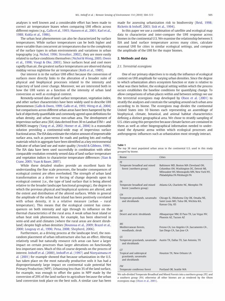
Table 1The top 38 most populated urban areas in the continental U.S. used in this studygrouped by biome.

Biome Cities

FETemperate broadleaf and mixedforest (northern group)

Baltimore MD, Boston MA Cleveland OH,Columbus OH, Washington DC, Detroit MI,Milwaukee WI, Minneapolis MN, New York NY,Philadelphia PA Pittsburgh PA

FATemperate broadleaf and mixedforest (southern group)

Atlanta GA, Charlotte NC, Memphis TN

GNTemperate grasslands, savannahsand shrublands

Chicago IL, Oklahoma City OK, Omaha NE,Saint Louis MO, Tulsa OK, Wichita KA,Kansas City, KS

DEDesert and xeric shrublands Albuquerque NM, El Paso TX, Las Vegas NV,

Phoenix AZ, Tucson AZ

MSMediterranean forests,woodlands, shrub

Fresno CA, Los Angeles CA ,Sacramento CA ,San Diego CA, San Jose CA

GSTemperate grasslands, savannahsand shrublands

Austin TX, Dallas TX, San Antonio, TX

GTTropical and subtropicalgrasslands, savannahsand shrublands

Houston TX, New Orleans LA

FWTemperate coniferous forest Portland OR, Seattle WA

We sub-divided Temperate Broadleaf andMixed Forests into a northern group (FE) anda southern group (FA) otherwise all other biomes are as rendered by the Olsonecoregions map (Olson et al., 2001).

505M.L. Imhoff et al. / Remote Sensing of Environment 114 (2010) 504–513

analyses is well known and a considerable effort has been made tocorrect air temperature biases when comparing UHI effects acrossdifferent regions (e.g., Gallo et al., 1993; Hansen et al., 2001; Karl et al.,1988; Kukla et al., 1986).

The urban heat phenomenon can also be characterized by surfacetemperatures. While surface temperatures can be both higher andmore variable than concurrent air temperatures due to the complexityof the surface types in urban environments and variations in urbantopography (e.g. Nichol, 1996; Streutker, 2002), they are more easilyrelated to surface conditions themselves (Nichol &Wong, 2005; Owenet al., 1998; Voogt & Oke, 2003). Since surfaces heat and cool morerapidly than air, the greatest surface temperatures are observed duringmidday versus nighttime for air temperature (Roth et al., 1989).

Our interest is in the surface UHI effect because the conversion ofsurfaces more directly links to the alteration of a broader suite ofphysical and biophysical processes related to the intensity andtrajectory of land cover change. Moreover, we are interested both inhow the UHI varies as a function of the intensity of urban landconversion as well as ecological context.

Remotely-sensed data of land surface temperature, vegetation index,and other surface characteristics have been widely used to describe UHIphenomenon (Gallo & Owen, 1999; Gallo et al., 1993; Weng et al., 2004)but comparisons across different urban areas have been hampered by thelack of objectively quantifiable and commonly agreedupondefinitions forurban density, and urban versus non-urban area. The development ofimpervious surface area (ISA) data derived from30mLandsat ETM+andIKONOS imagery (Yang et al., 2002; Homer et al., 2004) is a reasonablesolution providing a continental-wide map of impervious surfacefractional areas. The ISAdataestimate the relativeamountof impenetrablesurface area, such as pavements for roads and parking lots and roofingmaterialswhich in aggregate have been identified as a key environmentalindicator of urban land use and water quality (Arnold & Gibbons, 1996).The ISA data have been used successfully in combination with othercomparable resolution remotely sensed data of land surface temperatureand vegetation indices to characterize temperature differences (Xian &Crane, 2005; Yuan & Bauer, 2007).

While these detailed studies provide an excellent basis forunderstanding the fine scale processes, the broader consequences ofecological context are often overlooked. The strength of urban landtransformation as a driver or forcing of change depends upon itsecological context (i.e., the type of land surface that is being alteredrelative to the broader landscape functional groupings), the degree towhich the previous physical and biophysical systems are altered, andthe extent and distribution of the altered surfaces. While in generalthe amplitude of the urban heat island has been positively correlatedwith urban density, it is a relative measure (urban – ruraltemperature). This means that the ecological context has conse-quences on both intensity and sign through its influence on thethermal characteristics of the rural area. A weak urban heat island orurban heat sink phenomenon, for example, has been observed insemi-arid and arid climates (where the rural areas are desert shrub-land) despite high urban densities (Bounoua et al., 2009; Brazel et al.,2000; Lougeay et al., 1996; Pena, 2008; Shepherd, 2006).

Furthermore, as a driving process at the landscape level, the non-random placement of urban infrastructure also has an effect. Alteringrelatively small but naturally resource rich areas can have a largerimpact on certain processes than larger alterations on functionallyless important ones. Much of this of course depends on the process ofinterest. Imhoff et al. (2000), Imhoff et al. (1997) and Nizeyaimana etal. (2001) for example showed that because urbanization in the U.S.has taken place on the most naturally productive soils it has had adisproportionately large impact on continental scale potential NetPrimary Production (NPP). Urbanizing less than 3% of the land surface,for example, was enough to offset the gains in NPP made by theconversion of 29% of the land surface to agriculture because the urbanland conversion took place on the best soils. A similar case has been

made for assessing urbanization risk to biodiversity (Reid, 1998;Ricketts & Imhoff, 2003; Sisk et al., 1994).

In this paper we use a combination of satellite and ecological mapdata to characterize and inter-compare the UHI response acrossbiomes in the continental U.S.We examine the relationship between %ISA and land surface temperature across many cities, calculateseasonal UHI for cities in similar ecological settings, and comparethe amplitude of the UHI for the major biomes.

2. Methods and data

2.1. Terrestrial ecoregions

One of our primary objectives is to study the influence of ecologicalcontext on UHI amplitude for varying urban densities. Since the degreeto which urbanization alters ecosystem function or state is relative towhat was there before, the ecological setting within which the processoccurs establishes the baseline conditions for quantifying change. Toallow comparisons of urban places within and between settings we usethe terrestrial ecoregions map developed by Olson et al. (2001) tostratify the analyses and constrain the sampling around each urban areaaccording to its biome. The ecoregions map divides the continentalUnited States into 10 biomes each representing an assemblage ofbiophysical, climate, botanical, and animal habitat characteristicsdefining a distinct geographical area. We chose to stratify sampling ofU.S. cities using this perspective because climate factors are contained inthem as well as other biogeographical information needed to under-stand the dynamic arena within which ecological processes andanthropogenic influences such as urbanization most strongly interact.

506 M.L. Imhoff et al. / Remote Sensing of Environment 114 (2010) 504–513

In this study we analyze data for 38 of the most populated urbanareas in the continental United States occurring across six of thelargest biomes. We further subdivide two of the larger biomes in theset (Temperate Broadleaf and Mixed Forest and Temperate Grass-lands, Savannas and Shrublands) differentiating Northeast and Mid-Atlantic forest and Northern versus Southern Mid-western grasslands(Table 1). In this study, all temperature and NDVI data collected for anindividual urban area is included in the analysis only if they remain inthe dominant biome. This eliminates cross-over into different bio-climatic environments as a potential contaminant of the observedtemperature differences within an urban area and allows groupingand comparison of UHI effects by biome.

2.2. Classification of urban density

We use the impervious surface area (ISA) data from the Landsat-derived, continental scale land cover map (NLCD) in a GeographicInformation System-based spatial analysis to identify individual urbanareas, stratify them internally according to ISA density, and estimatetheir size. The fractional area impervious surfacedatawerederivedusingLandsat 7 ETM+ and IKONOS differentiating man-made surfaces fromnatural or vegetated surfaces (see Yang et al., 2002). While thisparameter does not contain retrievable information about albedo or 3-D structure, it captures development intensity as a function of the extentand spatial distribution of the collection of man-made surfaces within apixel. Conversion intensity based on ISA can be related to changes in the

Fig. 1. Urban area definition using impervious surface area (ISA) thresholds on the NLCD 20Panel B shows 676 urban polygons defined by 50% imperviousness contour; Panel C showsdefine the urban–suburban boundary. Panel D shows the close spatial matching between thspatial overlap ensures that the emissivities assigned to the MODIS LST split-window algoriUrban1, and Urban2).

biophysics of the land surface including sensible and latent heat fluxeswithin the urban surface and boundary layers through comparison withother spatially co-registered data.Most recently, Yuan and Bauer (2007)and Xian & Crane (2005) demonstrated that ISA data developed fromETM+ and the NLCD could be used to make rigorous comparisons ofurbandensity and surface temperature at local scales suggestingbroaderapplication would be possible with appropriate temperature data.

We use a 25% ISA threshold to define polygons in the Landsat-basedthematic data. The 25% threshold identifies a reasonable boundarybetween urban and low intensity residential lands (Lu & Weng, 2006)and provides reasonably spatially coherent urban groupings (Fig. 1). Assuch the polygons we define here overlap named cities but do notnecessarily match incorporated or cadastral (administrative) bound-aries. Most important; however, is the close match between the areadefined by the 25% ISA threshold and the MODIS landcover mapclassifyingUrbanBuilt-Up land (Fig. 1d).MODIS LST retrieval algorithmsrely on thismap for estimating surface emissivity (Wan et al., 2004) so aclose match here ensures that temperature comparisons within theurban polygon are based on retrievals using the same parameter sets.

Once individual city place urban polygons are defined we furtherstratify the landscape within and around them using classes based onISA and distance. In this paper we define five zones based on classes of% ISA in concentric rings emanating outward from the highest ISA in acity to the lowest: 1) Urban Core=pixels having 75% to 100% ISA(these are the highest in a city polygon); 2) Urban1=pixels havingISA between 75% and 50% (75%>ISA≥50%); 3) Urban2=pixels

01 dataset. Panel A shows one uninterrupted city polygon defined by 25% ISA contour;5300 polygons defined by 75% imperviousness contour. We use the 25% ISA contour toe 25% ISA contour and the MODIS landcover class for urban and built-up land. The closethm for temperature retrieval are the same within the three urban zones (Urban Core,

507M.L. Imhoff et al. / Remote Sensing of Environment 114 (2010) 504–513

having between 50% and 25% ISA (50%>ISA≥25%) — this is the lasturban zone and its outer boundary identifies the 25% threshold;4) Suburban=pixels located in a buffer zone 0–5 km adjacent to andoutside the 25% ISA contour (pixels have less than25% ISA); and5) Rural(or non-urban)=pixels located in a 5 kmwide ring located between 45and 50 km away from the 25% ISA contour and having less than 5% ISA(Fig. 2a,b). This rural ring is chosen to be at an optimal distance farenough from the urban core to represent a remote rural area yet not toofar to infringe into the 25% contour of an adjacent urban area or anotherbiome. Pixels that fall into overlapping biomes, other urban areas ortopographic elevations ±50m off themean elevation of the urban coreare excluded from the analysis.

2.3. Land surface temperature (LST) and NDVI

To characterize the surface temperature and the presence ofvegetation within the ISA zones, we useMODIS-Aqua Version 5, 8-daycomposite (MOD11A2) LST with high quality control (Wan et al.,2004) and 16-day composite NDVI (Huete et al., 1994, 1997) at1km×1km resolution (both covering 2003 to 2005). LST's fromMOD11A2 are retrieved from clear-sky (99% confidence) observationsat 1:30 PM and 1:30 AM using a generalized split-window algorithm(Wan & Dozier, 1996). The coefficients used in the split windowalgorithm are given by interpolating a set of multi-dimensional look-

Fig. 2. Panels A and B show examples of the typical layout of the five urban zones defined forzone is composed of pixels with less than 25% ISA occurring within a 5 km wide ring adjacen25% ISA contour composed of pixels with less than 5% ISA. Pixels that cross biomes or signiMODIS LST averages from the Urban Core and Rural zones. Panel C shows the cities used in

up tables (LUT) derived by linear regression of MODIS simulation datafrom radiative transfer calculations over wide ranges of surface andatmospheric conditions. These look up tables have been continuouslyupgraded (Wan et al., 2004) and comparisons between MODIS LST'sand in-situ measurements across a wide set of test sites indicate theaccuracy is better than 1 Kwith an RMS (of differences) less than 0.5 Kin most cases (Wan, 2008; Wang et al., 2008).

The LST data are used to characterize the horizontal temperaturegradient across the urban area and NDVI is used to describe thevegetation density temporal variation for each urban zone. Asmentioned previously, temperature and NDVI data for each zone inan urban area are only collected if they remain in the dominant biomefor that city. This eliminates cross-over into different bio-climaticenvironments as a potential contaminant of the observed tempera-ture differences within an urban area and allows grouping andcomparison of UHI effects by biome.

2.4. Topographic and population data

Topographic data are used as a filter to exclude from the analysistemperature differences due to elevation and shading. We use the~925 m SRTM30 (Farr & Kobrick, 2000) dataset to determine a meanelevation of the urban area and exclude from analysis all pixels whoseelevation is outside the +/−50m window from the mean elevation.

each city. Urban Core, Urban1 and Urban2 are based on %ISA of each pixel. The Suburbant to the 25% ISA contour. The Rural zone is a ring that is 45–50 km in distance from theficant changes (±50 m) in elevation are excluded. UHI (urban–rural) calculations usethis analysis and their biomes according to Olson et al. (2001).

508 M.L. Imhoff et al. / Remote Sensing of Environment 114 (2010) 504–513

We also use the 30arc sec (~925 m) US Census Grids 2000(Deichmann et al., 2001) produced by the Center for InternationalEarth Science Information Network to characterize the population.

3. Results and discussion

3.1. The UHI and ecological context

Using the population data, we identified 38 of the most populatedurban areas in the continental United States distributed over eightdifferent biomes (Table 1, Fig. 2c). For each urban area, a spatialstratification defining the five ISA zones is applied. A 0.1 NDVIthreshold is used to exclude water, bare soil and other non-vegetatedpixels from the spatial and temporal average in the rural zone of eachurban area.

For all cities across the biomes, the impervious surface areadecreases from the urban core with about 80% average ISA to the ruralarea where all pixels have less than 5% ISA. Also, the averageimpervious surface fraction within the five zones identified in eachcity is remarkably similar indicating that the ISA zonal classification issufficiently consistent for inter-comparison (Fig. 3a). The averagesummer daytime MODIS land surface temperature (1:30 PM localtime averaged for June, July and August) for all cities and zones showthat temperatures increase with ISA in all cases except urban areas indesert and xeric shrubland ecoregions (DE) (Fig. 3b). Despite the

Fig. 3. Average remotely-sensed parameters of the five zones (see Fig. 2) for cities in each ofarea (%), Panel B shows the average summer (Jun–Aug) MODIS NDVI for each zone in each grsurface temperature derived from MODIS product.

difference in spatial resolution, the MODIS 1 km NDVI tracks the ISAdata remarkably well showing an increase outward from the urbancore in all biomes except DE which shows a convex pattern (Fig. 3c).The anomalous NDVI and LST patterns for desert and xeric shrublandcities is likely a result of increased vegetation and latent heat flux inless dense 50–25% urban and suburban fringe areas due to resource(water) augmentation in those areas. This pattern has been notedpreviously for U.S. desert cities using AVHRR (Imhoff et al., 2004) andLandsat (Xian & Crane; 2005).

In terms of the UHI, we calculated the average temperaturedifferences (Urban Core LST−Rural LST) for all the cities in eachbiome for summer (June/July/August) and winter (December/Janu-ary/February) daytime (1:30 PM) and nighttime (1:30 AM). The UHIresponses for the eight different biomeswere all significantly different(p=0.01) and clearly show the effect of ecological context onseasonal and diurnal UHI amplitudes (Fig. 4). As expected, withsurface temperatures the greatest temperature differences are notedin daytime (Roth et al., 1989). On average we found that the summerUHI was significantly larger than the winter UHI. Energy demand inmetropolitan areas is determined by a complex variety of factorsrelated to the nature of the demand, the spatial distribution of highdemand centers and numerous other factors. However, our resultssuggest that for residential areas potential increases in coolingrequirements in summer would more than offset gains realized byheating in winter. The amplitude of summer daytime UHI appears to

the eight biomes defined in this study. Panel A represents the fractional imperviousnessoup, and Panel C shows the average summer daytime (around 1:30 PM local time) land

Fig. 4. Average urban heat island for cities in the different biomes (please refer to Table 1 and Fig. 2 for the definition biomes). Urban temperature is chosen from the most innercontour (Urban Core) of each city and the Rural temperature is the average of all the non-impervious pixels (ISA<0.1%) in the outermost contour (45–50 km buffer ring).Temperature differences for four periods are examined; average summer (Jun–Aug) daytime LST (1:30 PM), average summer nighttime LST (1:30 AM), average winter (Dec–Feb)daytime, and average winter nighttime LST.

509M.L. Imhoff et al. / Remote Sensing of Environment 114 (2010) 504–513

be related to the standing biomass of the surrounding biomedecreasing from forests to grasslands and reversing to a heat sink indesert cities. The largest average summer daytime UHI (7 to 9 °C) forexample is noted for cities displacing temperate broadleaf, mixed, andtemperate coniferous forest biomes (FE, FA, and FW). In high biomassforested biomes, urban areas are surrounded by dense and tallvegetation which intercepts and re-evaporates precipitation at

Fig. 5. A comparison of remotely-sensed parameters of the five urban zones found for a city inshrublands (Las Vegas, Nevada, USA). Panel A represents the average imperviousness area (average summer daytime MODIS LST for each zone.

potential rates and diffuses water from the deep soil to theatmosphere during the process of photosynthesis, thus keeping thesurrounding regions much cooler than the less vegetated urban core.In contrast, urban areas dominated by shorter low biomass vegetationsuch as grassland, shrublands and savannah (groups GN, MS, GS andGT) produce a less intense UHI with amplitudes ranging from 4 to6 °C. In these regions, the zones surrounding the Urban Core are

temperate broadleaf andmixed forest (Baltimore, Maryland, USA) and desert and xeric%), Panel B shows the average summer (Jun–Aug) MODIS NDVI, and Panel C shows the

Fig. 6. Composite averaged summer (Jun–Aug) daytime LST profile from MODIS acrossall urban zones. Baltimore (black triangles) located in temperate forests and Las Vegas(black squares) in a desert. Averages are computed from 12 cross-sections obtained at15° interval and for 180° around the urban area. The entire profile is finally obtainedusing symmetry with respect to the urban center.

Table 2The linear parameters relating average summer (Jun–Aug) daytime (1:30 PM) MODISLST anomaly (dependent) and impervious surface area anomaly (independent) for the38 top population cities in the continental U.S. grouped by the biomes in which theyreside.

Biomes Linear fit

R2 Slope (with 95% confidence interval) P-value

All combined 0.70 0.073 <0.00010.066–0.080

FE 0.92 0.107 <0.00010.098–0.115

FA 0.86 0.092 <0.00010.069–0.114

GN 0.89 0.077 <0.00010.067–0.086

DE a a a

MS 0.80 0.078 <0.00010.061–0.095

GS 0.86 0.066 <0.00010.050–0.081

GT 0.73 0.058 0.0020.029–0.086

FW 0.86 0.092 <0.00010.062–0.122

Data for five zones are used in each city: 1) Urban Core (75%>ISA≥50%); 2) Urban1(75%>ISA≥50%); 3) Urban2 (50%>ISA≥25%); 4) suburban (pixels located in a bufferzone of 0–5 km adjacent to and outside the 25% ISA contour); and 5) Rural (non-urbanpixels located in a 5 kmwide ring located between 45 and 50 km away from the 25% ISAcontour). LST data were collected between 2003 and 2005.

a Linear fit is not significant for desert cities.

510 M.L. Imhoff et al. / Remote Sensing of Environment 114 (2010) 504–513

sparsely vegetated and restore an important part of the absorbed solarenergy as sensible heating; thus reducing the horizontal temperaturegradient between the Urban Core and the Rural Zone. In urban areassurrounded by deserts and xeric shrublands (DE) this temperaturecontrast weakens and even reverses. The summer daytime UHI datafor DE was actually slightly negative (−1 °C) and taken in isolation itwould tend to corroborate the heat sink effect noted for many desertcities. However, the summer nighttime and winter daytime andnighttime UHI's for DE are still positive and large enough to make thecities warmer overall than the outlying areas. Urban areas in the DEbiomewere also the only ones to consistently show a larger nighttimeUHI effect. To further examine the influence of ecological context wecompare average summer daytime LST across ISA zones for Baltimore,Maryland, located in the Northeastern Temperate Broadleaf andMixed Forest (group FE) and Las Vegas, Nevada, an urban area builtwithin the Desert and Xeric Shrubland biome and arid climateconditions (Fig. 5).

The twourbanareas are similarwith respect to theaverage fractionalISA found in each of the defined urban zones (Fig. 5a); however, thedensity of the vegetation surrounding them, as illustrated by the NDVI(Fig. 5b) is sharply different. The NDVI difference between the RuralZone and the Urban Core is 0.4 in Baltimore and less than 0.1 for LasVegas. In LasVegas; however, the vegetationdensity increases (initially)away from the Urban Core (e.g., Urban1, Urban2 and Suburban) thendrops again in the Rural Zone. This suggests that the less dense urbanzones (Urban2 and Suburban) in Las Vegas are supporting plant growth(e.g., exotic tree and shrub species and lawns through irrigation) at arate greater than that of the surrounding biome (Imhoff et al., 2004).These two cities demonstrate the importance of ecological context asamodulator of the UHI effect. While the urban core in Baltimore createsa well-defined UHI with amplitude of 9.3 °C, in Las Vegas, it points to apossible heat sink (about 0.5 °C — a small number relative to theaccuracy of the MODIS LST product). If only the Urban2 zone (50–25%ISA) in Las Vegas is compared to its rural zone, there is a temperatureincrease of 1.6 °C. These results at least trend in the direction of apotential heat sink effect for arid cities postulatedby some(e.g. Bounouaet al., 2009; Shepherd, 2005, 2006). Composite averaged summer dayLST profiles across theUrban Core for the two urban areas are illustratedin Fig. 6.

3.2. Quantifying the relationship between LST and ISA

We quantify the relationships between the fractional area ofimpervious surfaces and the UHI by analyzing the LST and ISAanomalies for all 38 urban areas. The close spatial overlap of theMODIS landcover (urban built-up) with the three urban zones wedefine in this study (Urban Core, Urban1 and Urban2) ensures that theemissivities assigned to the MODIS LST split-window algorithm fortemperature retrieval are mostly the same (Fig. 2d). Even though thedifferences in the emissivities are small this further reduces thepossibility of LUT induced signal in the comparison of LST's betweenISA zones (Wan, 2008).

For each urban polygon we compute the mean summer daytimeLST anomaly of each zone by subtracting from its LST the averageobtained over all five zones. As expected, changes in ISA fractionstrongly affect changes in LST. For all of the urban areas combined,changes in ISA control about 70% of the variance in LST. In general, at a0.001 significance level, about 60–90% of the variance in LST isexplained by changes in ISA and these results are well in line withsimilar comparisons of ISA and LST for the Twin Cities Metroplex inMinnesota (Yuan & Bauer, 2007). With the exception of DE, in generalthere is positive relationship between LST and ISA. We found the ISA/LST relationship to be strongest for urban areas in forested biomes(e.g., group FE, FA and FW) where variations in ISA explain more than85% of the variation in LST (Table 2, Fig. 7a). We also note that the rateof change in LST as a function of ISA is different for urban areas in

forested biomes forests versus those characterized by short vegeta-tion. For example, at 95% confidence limit, the slope of the linear fit is10% for temperate forested groups FE, FA, and FW while it is only 6%for shorter vegetations (e.g., group GN, MS, GS, and GT). This impliesthat the rate of temperature increase with ISA is influenced byecological context (i.e., regional climate, surrounding vegetation,soils) as well as its impervious surface fractional area drivenevaporation capacity. One possible explanation for this is that shortvegetation surrounding urban areas in the southern and central partsof the country will experience heat stress more quickly than forestvegetation. This would cause a more frequent reduction of thetranspiration rates in those biomes thereby increasing the surface

Fig. 7. The relationship between the ISA anomaly and the summer daytime LST anomaly for U.S. cities in temperate broadleaf and mixed forest (FE) and desert and xeric shrublands(DE). The response in all other biomes is similar to FE. The x-axis represents the ISA anomaly by subtracting the mean ISA of the zones for each city and the y-axis represents thesummer day LST anomaly by subtracting the mean LST for each city.

511M.L. Imhoff et al. / Remote Sensing of Environment 114 (2010) 504–513

temperature at canopy level and contribute to the attenuation of thethermal contrast between the urban core and the surroundings.

For the desert groups, a polynomial relationship better describesthe LST and ISA anomalies (Fig. 7b). The polynomial relationshipexplains about 26% of the LST variance in the five desert urban areas(group DE). Remarkably, however, if only Las Vegas and Phoenix areconsidered, more than 70% of the LST variance is explained by changesin ISA. This would indicate that there is considerable variation in theUHI response for desert cities possibly due to differences within thebiome or the physical characteristics of the urban surfaces such asalbedo and 3D structure not identifiable in the ISA data.

The heat island effect tends to be strongly dependent on thepresence of vegetation within the different urban zones. For instancein Las Vegas and Phoenix, the coolest summer surface temperature isfound in the third zone (Urban2) which has a fractional ISA between50% and 25% and the highest NDVI. From this zone, LST increases inboth directions (inward towards the urban hot core and outwardtowards the surrounding rural desert) by about 1 °C. The surfacetemperature in the urban core is similar to that of the desert for an ISAanomaly of about 40%.

Fig. 8. Temperature difference between urban and the surrounding rural region for 45sampled Northeast cities in four groups with different city area: 1–10 km2, 10–100 km2,100–1000 km2, and >1000 km2. Urban temperature is chosen from the most innercontour of each city and the rural temperature is the average of all the non-imperviouspixels (ISA<0.1%) in the most outer contour (15–20 km buffer ring). For each city,temperature differences for four different periods are examined: average summer (Jun–Aug) daytime LST (1:30 PM), average summer nighttime LST (1:30 AM), average winter(Dec–Feb) daytime LST, and average winter nighttime LST.

3.3. UHI and urban extent in temperate forest setting

To examine the relationship between the total size of the urbanarea and the amplitude of the UHI we compare the total area of eachurban polygon (summed areas of zones ISA 25% and greater) to theUrban Core–Rural temperature difference for 45 randomly selectedcities within the NE biome. This sample set includes those cities listedin Table 2 under FE plus 34 additional cities located in that biome. Sizein this case is the total contiguous area for an urban polygon definedby the 25% ISA threshold. We group the 45 cities based on size andanalyze diurnal and seasonal UHI (Fig. 8). Our analysis indicates thatfor cities within this biome, the summer daytime UHI is stronglycorrelated to size. For instance, the averaged UHI is about 1.5 °C forurban areas smaller than 10 km2, while it about 10 °C for urban areaslarger than 1000 km2 (Fig. 8). This relationship holds true during thewinter but with a much weaker UHI amplitude ranging from about2.0 °C for urban areas smaller than 10 km2 to 3.5 °C for urban areaslarger than 1000 km2. A similar pattern is observed during thenighttime. The difference between the summer and winter UHIamplitude is indicative of the vegetation function in these temperatemixed forests. During summer when vegetation is physiologically

active, the evaporative cooling is strong during the day and creates apronounced UHI between impervious and vegetated zones. Duringwinter, the contrast between the urban and rural zones is subduedwhen leaves are off and photosynthetic activity is down-regulated bycold temperatures. During summer nighttime, the UHI persists in allurban areas but with smaller amplitudes ranging from 1 °C for urbanareas less than 1 km2 to 3.5 °C for those urban areas larger than1000 km2. During winter nights, the UHI effect is less than 1 °C for thelargest urban area.

Within the Northeastern temperate broadleaf mixed forest biome,the relationship between the UHI amplitude and total urban area isconsistent among all of the cities (Fig. 9). The relationship betweenthe UHI amplitude and size is log–linear and is given by:

ΔTUrban–Rural = 3:48logðAreaÞ + 1:75

and explains about 71% of the variance in UHI with a standard error of±1.6 °C. This result is similar to the log–linear relationship between

Fig. 9. The relationship between urban heat island and urban area size in NortheasternU.S. urban areas. The urban area size is defined as the total area surrounded by the 25%imperviousness contour of each city.

512 M.L. Imhoff et al. / Remote Sensing of Environment 114 (2010) 504–513

the UHI and the population size described in Oke (1973, 1976) andLandsberg (1981) only here we relate it directly to the size of thetransformed surface (i.e., total area in a city having ISA≥25%).

4. Summary

In this study we combine remote sensing data from differentplatforms to assess the urban heat island amplitude and itsrelationship to urban spatial structure and size for a large number ofcities across a variety of eco-climatic regions over the continentalUnited States. We use a Landsat ETM+ and IKONOS based datasetestimating the fractional area of impervious surfaces at 30 m andcompare them to 1 km land surface temperature data from theMODISinstrument on the Aqua satellite for 38 of the most populous cities inthe continental United States.

In general we find that the fraction ISA is a good predictor of LSTfor all cities in the continental United States in all biomes exceptdeserts and xeric shrublands. The fraction of ISA explains about 70% ofthe total variance in LST for all cities combined with the highestcorrelations (90%) in the Northeastern U.S. where urban areas areembedded in temperate broadleaf and mixed forests. More impor-tantly, these correlations are consistent for small, medium and largeurban areas. In most biomes, the LST is linearly proportional to the ISAfraction. The relationship between temperature and ISA for urbanareas in deserts and xeric shrublands is more complicated requiring asecond order polynomial with large variations in outcome if theanalysis is conducted on fewer cities in the group. In desert typeecosystems suburban zones with moderate ISA fractions are coolerthan the surrounding rural desert fringe and the urban core where ISAis usually above 75%.

In terms ofUHI's andbiomes our results showthat ecological contextis a statistically significant modulator of the diurnal and seasonal UHI'sin the continental United States. The largest (urban–rural) temperaturedifferences for all biomes are found for summermidday and the greatestamplitudes are found for urban areas displacing forests (6.5–9.0 °C)followed by temperate grasslands (6.3 °C), and tropical grasslands andsavannas (5.0 °C) respectively. Urbanization initiates a differentialheating process between impervious surfaces, generally made ofconcrete and other heat absorbing materials, and the surroundingnaturally vegetated landscapes. The contrast between urban cores andrural zones is driven by the surrounding land use type and is oftenaccentuated during the time when the vegetation is physiologicallyactive, especially in forested lands. In biomes with short vegetation thecontrast is less. Similarly, the amplitude of the UHI is significantlydiminished during thewinter seasonwhen vegetation loses its leaves oris stressed by lower temperatures. Urban areas in deserts behave

differently showing very little change relative to their non-urbanizedsurroundings. Our data show an overall heat sink pattern similar to thatdescribed by previous studies (e.g., Brazel et al., 2000; Pena, 2008);however,while ourfindings are consistentwith theory, the temperaturedifferences we find here are small (between 0.2 and 2.2 °C) relative tothe known accuracy of theMODIS LST product. In this paper we begin acharacterization and inter-comparison of the UHI in the continentalUnited States from a biomes perspective. This approach allows a broad-scale appreciation of how ecological context influences UHI's. However,it does not reveal the complexities found in most urban environmentswhere significant ecological variation is present at the finer scale. Alogical next step to this characterization would be to use higher spatialresolutionbiome information capable of showing ecoregional variationswithin a city. Such an approach would permit city-scale investigationsabout the interplay betweenurban surfaces and their ecological settingsand their impact on UHI and other related environmental issues.

Finally, this research highlights a significant positive relationshipbetween the urban heat island magnitude, the size of the urban area,and ecological setting estimated entirely from remotely sensedobservations. The use of ISA as an estimator of the extent andintensity of urbanization is more objective than population densitybased methods and can be consistently applied across large areas forinter-comparison of impacts on biophysical processes. Overall, ourresults suggest that remotely-sensed land surface temperatureprovides an adequate characterization of both the magnitude andspatial extent of the urban heat island and allow objectivecomparisons of urban heat island effects around urban areas ofdifferent sizes at continental scales without the significant biasencountered in conventional ground observations.

References

Arnold, C. L., Jr., & Gibbons, C. J. (1996). Impervious surface coverage: The emergence ofa key environmental indicator. Journal of the American Planning Association, 62(2),243−258.

Bounoua, L., Safia, A., Masek, J., Peters-Lidard, C., & Imhoff, M. L. (2009). Impact of urbangrowth on surface climate: A case study in Oran, Algeria. Journal of AppliedMeteorology and Climatology, 48, 217−231.

Brazel, A., Selover, N., Vose, R., & Heisler, G. (2000). The tale of two climates-Baltimoreand Phoenix urban LTER sites. Climate Research, 15, 123−135.

Deichmann, U., Balk, D., and Yetman, G. (2001). Transforming population data forinterdisciplinary usages: from census to grid. Documentation for GPW Version 2available only at http://sedac.ciesin.columbia.edu/plue/gpw/GPWdocumentation.pdf

Farr, T. G., & Kobrick, M. (2000). Shuttle radar topography mission produces a wealth ofdata. American Geophysical Union EOS, 81, 583−585.

Gallo, K. P., McNab, A. L., Karl, T. R., Brown, J. F., Hood, J. J., & Tarpley, J. D. (1993). The useof NOAA AVHRR data for assessment of the Urban Heat Island effect. Journal ofApplied Meteorology, 32(5), 899−908.

Gallo, K. P., & Owen, T. W. (1999). Satellite-based adjustments for the urban heat islandtemperature bias. Journal of Applied Meteorology, 38, 806−813.

Grimmond, C. S. B., & Oke, R. (2002). Turbulent heat fluxes in urban areas: observationsand a Local-scale Urban Meteorological Parameterization Scheme (LUMPS). Journalof Applied Meteorology, 41, 792−810.

Hansen, J. E., Ruedy, R., Sato, M., Imhoff, M., Lawrence, W., Easterling, D., et al. (2001). Acloser look at United States and global surface temperature change. Journal ofGeophysical Research, 106, 23947−23963. doi:10.1029/2001JD000354

Homer, C., Huang, C., Yang, L., Wylie, B., & Coan, M. (2004). Development of a 2001national Land-Cover Database for the United States. Photogrammetric Engineering &Remote Sensing, 70(7), 829−840.

Huete, A. R., Justice, C., & Liu, H. (1994). Development of vegetation and soil indices forMODIS-EOS. Remote Sensing Environment, 49, 224−234.

Huete, A. R., Liu, H. Q., Batchily, K., & van Leeuwen, W. J. D. (1997). A comparison ofvegetation indices over a global set of TM images for EOS-MODIS. Remote SensingEnvironment, 59, 440−451.

Imhoff, M., Lawrence, W. T., Stutzer, D. C., & Elvidge, C. D. (1997). Using nighttimeDMSP/OLS images of city lights to estimate the impact of urban land use on soilresources in the US. Remote Sensing of Environment, 59, 105−117.

Imhoff, M. L., Tucker, C. J., Lawrence, W. T., & Stutzer, D. C. (2000). The use ofmultisource satellite and geospatial data to study the effect of urbanization onprimary productivity in the United States. IEEE Transactions on Geoscience andRemote Sensing, 38(6), 2549−2556.

Imhoff, M. L., Bounoua, L., DeFries, R., Lawrence, W. T., Stutzer, D., Tucker, C. J., et al.(2004). The consequences of urban land transformation on net primaryproductivity in the United States. Remote Sensing of Environment, 89, 434−443.

513M.L. Imhoff et al. / Remote Sensing of Environment 114 (2010) 504–513

Karl, T. R., Diza, H. F., & Kukla, G. (1988). Urbanization: its detection and effect in theUnited States climate record. Journal of Climate, 1, 1099−1123.

Kukla, G., Gavin, J., & Karl, T. R. (1986). Urban warming. Journal of Climate and AppliedMeteorology, 25, 1265−1270.

Landsberg, E. H. (1981). The urban climate. International Geophysics Series, Vol. 28. (pp. 5)New York: Academic Press.

Lougeay, R., Brazel, A., & Hubble, M. (1996). Monitoring intraurban temperaturepatterns and associated land cover in Phoenix, Arizona using Landsat thermal data.Geocarto International, 11, 79−90.

Lu, D., & Weng, Q. (2006). Use of impervious surface in urban land-use classification.Remote Sensing of Environment, 102, 146−160.

Manley, G. (1958). On the frequency of snowfall in metropolitan England. QuarterlyJournal of the Royal Meteorological Society, 84, 70−72.

Nichol, J. (1996). High-resolution surface temperature patterns related to urbanmorphology in a tropical city: a satellite-based study. Journal of AppliedMeteorology, 35(1), 135−146.

Nichol, J., & Wong, W. S. (2005). Modeling urban environmental quality in a tropicalcity. Landscape and Urban Planning, 73(1), 49−58.

Nizeyaimana, E., Petersen, G. W., Imhoff, M. L., Sinclair, H., Waltman, S., Reed-Margetan,D. S., et al. (2001). Assessing the impact of land conversion to urban use on soilswith different productivity levels in the USA. Soil Science Society of America Journal,65, 391−402.

Oke, T. R. (1973). City size and the urban heat island. Atmospheric EnvironmentPergamon Press, 7, 769−779.

Oke, T. R. (1976). The distinction between canopy and boundary layer urban heatislands. Atmosphere, 14, 268−277.

Olson, D. M., Dinerstein, E., Wikramanayake, E. D., Burgess, N. D., Powell, G. V. N.,Underwood, E. C., et al. (2001). Terrestrial Ecoregions of the World: A New Map ofLife on Earth. BioScience, 51(11), 933−938.

Owen, T. W., Carlson, T. N., & Gillies, R. R. (1998). An assessment of satellite remotely-sensed land cover parameters in quantitatively describing the climatic effect ofurbanization. International Journal of Remote Sensing, 19(9), 1663−1681.

Quattrochi, D., & Ridd, M. K. (1994). Measurement of thermal energy properties ofcommon urban surfaces using the thermal infrared multispectral scanner. Inter-national Journal of Remote Sensing, 15(10), 1991−2022.

Pena, M. A. (2008). Relationships between remotely sensed surface parametersassociated with the urban heat sink formation in Santiago, Chile. InternationalJournal of Remote Sensing, 29(15), 4385−4404.

Reid, W. V. (1998). Biodiversity hotspots. Trends in Ecology and Evolution, 13, 275−280.Ricketts, T., & Imhoff, M. (2003). Biodiversity, urban areas, and agriculture locating

priority ecoregions for conservation.Conservation Ecology, 8(2), 1 URL: http://www.consecol.org/vol8/iss2/art1/

Rosenzweig, C., Solecki, W. D., Parshall, L., Chopping, M., Pope, G., & Goldber, R. (2005).Characterizing the urban heat island in current and future climates in New Jersey.Environmental Hazards, 6, 51−62. doi:10.1016/j.hazards.2004.12.001

Roth, M., Oke, T. R., & Emery, W. J. (1989). Satellite-derived urban heat islands fromthree coastal cities and the utilization of such data in urban climatology. Interna-tional Journal of Remote Sensing, 10, 1699−1720.

Shepherd, J. M. (2005). A review of current investigations of urban-induced rainfall andrecommendations for the future. Earth Interactions, 9(1), 1−27.

Shepherd, J. M. (2006). Evidence of urban-induced precipitation variability in aridclimate regimes. Journal of Arid Environments, 67, 607−628.

Shepherd, J. M., & Burian, S. J. (2003). Detection of urban-induced rainfall anomalies inmajor coastal city. Earth Interactions, 7(4), 1−17.

Sisk, T. D., Launer, A. E., Switky, K. R., & Ehrlich, P. R. (1994). Identifying extinctionthreats. BioScience, 44, 592−604.

Streutker, D. R. (2002). A remote sensing study of urban heat island of Houston, Texas.International Journal of Remote Sensing, 23(13), 2595−2608.

Trenberth, K. E., Jones, P. D., Ambenje, P., Bojariu, R., Easterling, D., Klein Tank, A., et al.(2007). Observations: Surface and atmospheric climate change. Climate Change2007: The Physical Science BasisIn S. Solomon, D. Qin, M. Manning, Z. Chen, M.Marquis, K. B. Averyt, M. Tignor, & H. L. Miller (Eds.), Contribution of Working GroupI to the Fourth Assessment Report of the Intergovernmental Panel on Climate ChangeCambridge: Cambridge University Press.

UNFPA (2007). The state of world population 2007: Unleashing the potential of urbangrowth. United Nations Population Fund, United Nations Publications 1 pp.

Voogt, J. A., & Oke, T. R. (2003). Thermal remote sensing of urban climates. RemoteSensing Environment, 86, 370−384.

Wan, Z., & Dozier, J. (1996). A generalized split-window algorithm for retrieving land-surface temperature from space. IEEE Transactions on Geoscience and RemoteSensing, 34(4), 892−905.

Wan, Z., Zhang, Y., Zhang, Q., & Li, Z. -L. (2004). Quality assessment and validation of theMODIS land surface temperature. International Journal of Remote Sensing, 25,261−274.

Wan, Z. (2008). New refinements and validation of the MODIS land-surfacetemperature/emissivity products. Remote Sensing of Environment, 112, 59−74.

Wang, W., Liang, S., & Meyers, T. (2008). Validating MODIS land surface temperatureproducts using long-term nighttime ground measurements. Remote Sensing ofEnvironment, 112(3), 623−635.

Weng, Q., Dengsheng, L., & Jacquelyn, S. (2004). Estimation of land surfacetemperature–vegetation abundance relationship for urban heat island studies.Remote Sensing of Environment, 89, 467−483.

Xian, G., & Crane, M. (2005). Assessments of urban growth in the Tampa Bay watershedusing remote sensing data. Remote Sensing of Environment, 97, 203−215.

Yang, L., Huang, C., Homer, C., Wylie, B., & Coan, M. (2002). An approach for mappinglarge-area impervious surfaces: Synergistic use of Landsat 7 ETM+ and high spatialresolution imagery. Canadian Journal of Remote Sensing, 29(2), 230−240.

Yuan, F., & Bauer, M. E. (2007). Comparison of impervious surface area and normalizeddifference vegetation index as indicators of surface urban heat island effects inLandsat imagery. Remote Sensing of Environment, 106(3), 375−386.