Embed Size (px)
Citation preview

Remote sensing of CO2: Geostatistical tools for assessing spatial variability, quantifying representation
errors, and gap-filling
by
Alanood A A A Alkhaled
A dissertation submitted in partial fulfillment of the requirements for the degree of
Doctor of Philosophy (Environmental Engineering) in The University of Michigan
2009
Doctoral Committee:
Assistant Professor Anna Marta Michalak, Chair Professor Jonathan W. Bulkley Professor Richard B. Rood Professor Donald Scavia

ACKNOWLEDGEMENTS
First, I thank Allah for his generosity towards me during my entire life.
I thank my advisor, Prof. Anna Michalak, for her support, guidance and direction during
my PhD years. I learned from Anna and I am greatly inspired and thankful for the great
effort and attention that she gave me and that she gives all her students.
I thank Prof. Jonathan Bulkley, for his continuous direction and encouragement, and my
committee, Prof. Jonathan Bulkley, Prof. Richard Rood and Prof. Don Scavia for their
inputs and directions that helped improve this dissertation.
I thank my parents for their endless support, patience, faith and encouragement that
helped me complete this dissertation.
I would like to thank Kuwait University, and my country, for providing me with the
opportunity of studying at the University of Michigan, for supporting me financially and
for trusting me with a future position at Kuwait University.
ii
Portions of this work were adapted from the following manuscripts:
• Alkhaled, A. A., A. M. Michalak, and S. R. Kawa (2008), Using CO spatial
variability to quantify representation errors of satellite CO retrievals2
2 ,
Geophysical research letters, 35, L16813, doi:10.1029/2008GL034528.
• Alkhaled, A. A., A. M. Michalak, S. R. Kawa, S. C. Olsen, and J.-W. Wang
(2008), A global evaluation of the regional spatial variability of column integrated
CO2 distributions, Journal of Geophysical Research, 113, D20303,
doi:10.1029/2007JD009693.
The co-authors of these manuscripts are gratefully acknowledged.
iii

Table of Contents
ACKNOWLEDGEMENTS ..........................................................................................................ii
List of Figures................................................................................................................................ ix
List of Tables ................................................................................................................................xii
ABSTRACT.................................................................................................................................xiii
CHAPTER 1: INTRODUCTION................................................................................................. 1
Objective 1: Quantifying Regional X Variability .............................................................. 4co2
Objective 2: Evaluating the spatial representation errors of X retrievals .......................... 5CO2
Objective 3: Gap-filling X retrievals using flexible non-stationary covariances............... 6CO2
CHAPTER 2: BACKGROUND ................................................................................................... 9
1. The Carbon Cycle and CO measurements ................................................................... 92
1.1. Scientific need and applications .............................................................................. 9
1.2. The Orbiting Carbon Observatory ......................................................................... 11
2. X variability ................................................................................................................ 14CO2
2.1. Surface CO variability.......................................................................................... 142
2.2. Variability of column integrated CO dry-air mole fraction (X )....................... 192 CO2
2.2.1. Remote sensing of X .................................................................................. 20CO2
2.2.2. Model simulations vs. aircraft and FTS ......................................................... 23
3. Mapping missing observations in geophysical data ..................................................... 26
iv

3.1. Expectation-Maximization methods ...................................................................... 27
3.2. Empirical orthogonal functions methods............................................................... 29
3.3. Other statistical methods........................................................................................ 31
4. Geostatistical analysis ..................................................................................................... 33
4.1. Modeling spatial random functions ....................................................................... 33
4.2. Modeling of spatial variability............................................................................... 36
4.2.1. Random functions and stationarity ................................................................ 36
4.2.2. The auto-covariance and the semi-variogram ............................................... 38
4.3. Non-stationary spatial variability........................................................................... 41
4.3.1. Global and local methods for modeling non-stationary random functions ... 42
4.3.2. Intrinsic random functions of order k (IRF-k)................................................ 44
4.3.3. Multi-resolution modeling of spatial variability ............................................ 46
4.4. Support effect on modeled variability ................................................................... 49
4.5. Best Linear Unbiased Estimation (BLUE) ............................................................ 51
4.5.1. Ordinary Kriging (OK) .................................................................................. 51
4.5.2. Representation errors (Block Kriging) .......................................................... 52
4.5.3. Kriging non-stationarity and high frequency data......................................... 54
CHAPTER 3: A Global Evaluation of the Regional Spatial Variability of Column
Integrated CO Distributions2 ...................................................................................................... 58
1. Introduction ..................................................................................................................... 58
2. Methods............................................................................................................................ 61
2.1. MATCH/CASA model .......................................................................................... 61
2.2. Spatial variability................................................................................................... 63
2.2.1. Semi-variogram model ................................................................................... 63
v

2.2.2. Spatial variability analysis............................................................................. 65
2.3. Comparison to other models and aircraft data ....................................................... 69
2.3.1. PCTM/GEOS-4 global model......................................................................... 70
2.3.2. SiB-RAMS regional model ............................................................................. 71
2.3.3. Aircraft data ................................................................................................... 73
3. Results and discussion..................................................................................................... 74
3.1. Global X variability .......................................................................................... 74CO2
3.2. Regional X variability....................................................................................... 79CO2
3.2.1. Regional variance .......................................................................................... 79
3.2.2. Regional correlation lengths.......................................................................... 82
3.2.3. Sub-monthly temporal variability................................................................... 85
3.2.4. Overall variability .......................................................................................... 85
3.3. Comparison to other models and aircraft data ....................................................... 90
3.3.1. PCTM/GEOS-4 global simulation ................................................................. 90
3.3.2. SiB-RAMS regional simulation ...................................................................... 96
3.3.3. Aircraft data ................................................................................................. 100
4. Conclusions .................................................................................................................... 102
CHAPTER 4: Using CO Spatial Variability to Quantify Representation Errors of Satellite
CO Retrievals
2
2 ............................................................................................................................ 106
1. Introduction ................................................................................................................... 106
2. Data and methods.......................................................................................................... 110
2.1. Methods ............................................................................................................... 110
2.2. X spatial variability......................................................................................... 113CO2
2.3. Model gridcell and sampling conditions ............................................................. 114
vi

3. Results and discussion................................................................................................... 117
4. Conclusions .................................................................................................................... 124
CHAPTER 5: Gap-filling X Retrievals Using Flexible Non-Stationary Covariance
Functions
CO2
..................................................................................................................................... 126
1. Introduction ................................................................................................................... 126
2. Methods.......................................................................................................................... 132
2.1. Data...................................................................................................................... 132
2.1.1. PCTM/GEOS-4 ............................................................................................ 133
2.1.2. CALIPSO clouds and aerosols..................................................................... 134
2.1.3. Simulated OCO retrievals ............................................................................ 135
2.2. Gap-filling ........................................................................................................... 136
2.2.1. Statistical model:.......................................................................................... 136
2.2.2. Fixed rank Kriging (FRK)............................................................................ 141
2.2.3. Parameter optimization................................................................................ 143
3. Results and discussion................................................................................................... 149
3.1. Gap-filled OCO maps .......................................................................................... 149
3.2. Performance evaluation ....................................................................................... 151
3.3. Factors affecting map quality .............................................................................. 153
4. Conclusions .................................................................................................................... 158
CHAPTER 6: Conclusions and Future Directions ................................................................. 169
1. Conclusions .................................................................................................................... 169
2. Future directions ........................................................................................................... 173
2.1. X covariance analysis and representation error .............................................. 173CO2
vii

2.2. Statistical modeling of X ................................................................................ 174 CO2
2.3. Impact of presented and future work on carbon cycle science ............................ 175
2.4. Using geostatistics to improve the modeling of environmental processes .......... 177
BIBLIOGRAPHY...................................................................................................................... 179
viii

List of Figures
Figure 2.1: The Orbiting Carbon Observatory Track (OCO) 13 Figure 2.2: (a) 8-day and (b) 16-day simulated OCO observation locations during the period from January 17st to February 1st, 2007. Gaps are at locations that are out of OCO track or with clouds and aerosols optical thickness exceeding 0.1, as measured by the CALIPSO satellite (see chapter 5). Colorbars show model simulated XCO2 from the PCTM/GEOS-4 model (see chapter 5) during the period from January 17st to February 1st 2003. Differences in years are due to limited CALIPSO data availability 13 Figure 2.3: The binned experimental semi-variogram cloud and the fitted exponential semi-variogram function 40
Figure 3.1: The regional spatial covariance evaluates the spatial variability of XCO2 values within a region (e.g. Eastern North America – upper left) and between this region and global XCO2 values (lower right) 67
Figure 3.2: Global spatial covariance function parameters (variance and correlation length) of MATCH/CASA simulated XCO2 at 1pm local time evaluated daily and smoothed using a one week moving average 76
Figure 3.3a: Regional variance of MATCH/CASA simulated XCO2 at 1pm local time on the 15th of each month. Note differences in color scales. Regions are defined as 2000 km radius circles centered at the 2048 MATCH/CASA model gridcells 81
Figure 3.3b: Regional correlation length of MATCH/CASA simulated XCO2 at 1pm local time on the 15th of each month. Regions are defined as 2000 km radius circles centered at the 2048 MATCH/CASA model gridcells 84
Figure 3.4: Information scale ho based on MATCH/CASA regional spatial covariance structure for 0.5 ppm uncertainty level 87
ix

Figure 3.5: PCTM/GEOS-4 XCO2 regional variance (column a), regional correlation length (column b), and overall information scale (ho) for 0.5 ppm uncertainty level (column c). All columns are evaluated at 1pm local time,on the 15th of January, April, July and October 94
Figure 3.6: Average total CO2 fluxes (CASA biosphere, ocean and fossil fuel) for the month of October, and its regional variance and correlation length 95 Figure 3.7: Regional variance (a and c) and correlation length (b and d) of PCTM/GEOS-4 simulated XCO2 created by transporting: biospheric fluxes (first row), and fossil fuel fluxes (second row). PCTM/GEOS-4 XCO2 are evaluated at 1pm local time,on the 15th of October 95 Figure 4.1: 1°×1° model gridcell at 45° latitude discretized into 3km2 pixels representing the resolution at the scale of satellite sounding footprints. Dark gray pixels illustrate a single 8 pixel North-South swath through the middle of the gridcell. The black pixel represents a single satellite retrieval in the corner of the gridcell 116 Figure 4.2: January representation errors; (a) one sounding per gridcell, (b)
one swath per gridcell 122
Figure 4.3: July representation error; (a) one sounding per gridcell, (b) one swath per gridcell 123
Figure 5.1: Aerosol and clouds total optical depth for the months of (a) January 2007 and (b) July 2007 as measured by CALIPSO (white gridcells indicate data in availability or the failure to identify a single layer below 9km elevation) 135
Figure 5.2: (a) locations of the centers (xil) of 4 levels of the bi-square basis functions, and (b) An equatorial one dimensional cross-section of 3 levels of the bi-square basis for half the equator. Levels 1, 2 and 3 are represented by blue, red and black lines, respectively. 140
Figure 5.3: PCTM/GEOS-4 local temporal standard deviations at 8 and 16
days temporal lag 155
Figure 5.4: Average XCO2 distribution for (a) January 17th to January 24th
2003, and (b) January 17th to February 1st 2003 161
x

Figure 5.5: Gap-filling results and simulated retrievals for January 8-day
test cases: (a,e) simulated OCO samples, (b,f) gap-filled XCO2, (c,g) gap-filling uncertainty (expressed as one kriging standard deviation), (d,h) gap-filled XCO2 minus the true average modeled XCO2 over the sampled period 162
Figure 5.6: Gap-filling results and simulated retrievals for January 16-day
test cases: (a,e) simulated OCO samples, (b,f) gap-filled XCO2, (c,g) gap-filling uncertainty (expressed as one kriging standard deviation), (d,h) gap-filled XCO2 minus the true
average modeled XCO2 over the sampled period 163 Figure 5.7: Distribution of normalized gap-filling residuals for January test cases 164 Figure 5.8: Average XCO2 distribution for (a) July 1st to July 8th 2003, and (b) July 1st to July 16th 2003 165 Figure 5.9: Gap-filling results and simulated retrievals for July 8-day test
cases: (a,e) simulated OCO samples, (b,f) gap-filled XCO2, (c,g) gap-filling uncertainty (expressed as one kriging standard deviation), (d,h) gap-filled XCO2 minus the true
average modeled XCO2 over the sampled period 166 Figure 5.10: Gap-filling results and simulated retrievals for July 16-day
test cases: (a,e) simulated OCO samples, (b,f) gap-filled XCO2, (c,g) gap-filling uncertainty (expressed as one kriging standard deviation), (d,h) gap-filled XCO2 minus the true
average modeled XCO2 over the sampled period 167
Figure 5.11: Distribution of normalized gap-filling residuals for July test cases 168
xi

List of Tables
Table 3.1: Parameter ho for coincident regions and periods for MATCH/CASA global simulation, PCTM/GEOS-4 global simulation, SiB-RAMS regional model, and in-situ aircraft measurements. Note that reported ho values correspond to different months within the indicated range due to data availability 99 Table 5.1: OCO gap-filling test cases 132 Table 5.2: Results of gap-filling performance tests 153
xii

ABSTRACT
Remote sensing of CO2: Geostatistical tools for assessing spatial variability, quantifying representation
errors, and gap-filling
by
Alanood A A A Alkhaled
Chair: Anna Marta Michalak
Currently, approximately half of the anthropogenic emissions of CO2 are absorbed by
oceans and the terrestrial biosphere, thus greatly reducing the rate of atmospheric CO2
increase and related climate change. The current understanding of the global carbon
cycle, and of the sustainability of natural carbon sinks, is limited, however. To enhance
this knowledge, scientists use process-based biospheric models and atmospheric transport
models, together with the limited global ground-based CO2 measurement network to infer
global CO2 fluxes. Current estimates of carbon budgets at regional to continental scales
vary significantly, however, in large part due to limited atmospheric observations of CO2.
xiii

Satellite-based observations provide the possibility of global coverage of column-
averaged CO2 (XCO2), which could improve the precision of estimated CO2 fluxes. XCO2
observations will have large data gaps, however, which will limit the use of XCO2
observations for evaluating CO2 flux estimates. In addition, remote sensing soundings
will often be representative of fine scales relative to the resolution of typical atmospheric
transport models, causing representation errors that should be quantified for accurate CO2
flux estimation.
In this dissertation, the spatial variability of the XCO2 signal is quantified using
geostatistical analysis. Geostatistical methods that depend on the knowledge of this
spatial variability are then presented for evaluating representation errors. Unlike previous
estimates of representation errors, the proposed method accounts for the regionally-
variable XCO2 spatial variability, and the spatial distribution of retrievals. Further, a
spatial mixed-effects statistical model that best represents the quantified XCO2 variability
is presented for gap-filling XCO2 retrievals. The presented geostatistical gap-filling
method, which is based on a multi-resolution model of the spatial trend and variability of
XCO2, is tested using eight realistic scenarios of expected spatial distributions of XCO2
retrievals. The method yields XCO2 estimates over regions with data gaps, together with
an estimate of the associated gap-filling uncertainties.
The presented methods provide flexible tools that can be applied to estimate
representation errors and gap-fill XCO2 or other remotely sensed data. As such, they
xiv

provide the potential for improving and evaluating estimated CO2 fluxes, process-based
models, and atmospheric transport models.
xv
CHAPTER 1
INTRODUCTION
Increasing anthropogenic emissions of greenhouse gases (GHGs) are changing climate
patterns as well as the frequency and intensity of extreme weather events. Anthropogenic
emissions of carbon dioxide (CO2) are causing most of the increase in the Earth radiative
forcing relative to other GHGs. Prior to the industrial era, natural concentrations of
atmospheric CO2 had stable levels on decadal time scales with minor natural fluctuations.
During this century, anthropogenic emissions from fossil fuel burning, cement
manufacture and land use change have caused an increase in atmospheric CO2
concentrations. However, the present rate of increase of atmospheric CO2 represents only
half the anthropogenic emissions to the atmosphere. The other half is absorbed by the
ocean and the terrestrial biosphere, which act as natural sinks of carbon dioxide [Denman
et al., 2007]. Important scientific challenges include linking fluctuations of CO2 levels to
particular causes, and understanding the mechanisms governing these natural CO2 sinks
[Denman et al., 2007], both of which are critical for determining the sustainability of
natural sinks of CO2, as well as their reaction to the increasing CO2 concentrations and to
a changing climate.
1

Analysis of the spatial and temporal distribution and variability of carbon fluxes can
isolate and identify these mechanisms, and therefore improve the ability to model and
predict atmospheric CO2 levels. Such analysis, however, requires global CO2 data with
dense coverage, which does not presently exist. Satellite measurements of atmospheric
CO2 concentrations are a promising source of this highly needed global information.
Present remote sensing of atmospheric CO2 includes data from instruments such as the
SCanning Imaging Absorption spectroMeter for Atmospheric CHartographY
(SCIAMACHY) onboard the Environmental Satellite (ENVISAT) [Buchwitz et al.,
2005b], the Atmospheric Infrared Sounder (AIRS) onboard the Aqua satellite
[Chevallier et al., 2005a ] and the Television Infrared Observation Satellite (TIROS)
Operational Vertical Sounder (TOVS) [Chevallier et al., 2005b]. The utility of these data
products to carbon cycle science, however, is limited because of relatively high
measurement errors, biases, low resolutions, and large data gaps. More importantly, these
satellites provide only limited information about CO2 variability near the earth surface
(i.e. in the lower troposphere), where strong signals from the carbon fluxes exist.
Present efforts to overcome these limitations include the launch of two new satellites, the
Orbiting Carbon Observatory (OCO) [Crisp et al., 2004; Miller et al., 2007] and the
Greenhouse Gases Observing SATellite (GOSAT) [National Institute for Environmental
Studies-Japan, 2006]. These new satellites are capable of measuring column-averaged
CO2 dry air mole fraction (XCO2) with high sensitivity to near surface CO2 variations. The
new satellites are also designed to have small sounding footprints (3km2 for OCO and
2

100km2 for GOSAT) to improve the probability of obtaining XCO2 observations over
regions with high aerosol and cloud Optical Depth (OD), thus providing the improved
XCO2 information and coverage that are required to advance carbon cycle science.
Some of the XCO2 variability captured by high resolution XCO2 retrievals will not be
represented by current transport models, however, because of current models’ relatively
coarse resolution ( typical model resolution between 104 km2 – 106 km2 [Miller et al.,
2007]). The inability of transport models to represent XCO2 as measured by OCO is
expected to be particularly evident over high XCO2 variability areas, such as in the vicinity
of strong biospheric fluxes. Therefore, using high resolution XCO2 retrievals in carbon
cycle studies requires the quantification of the levels of mismatch between the
observations and the modeled concentrations (i.e. representation errors).
Another difficulty associated with using OCO and GOSAT data to estimate CO2 fluxes
are the imperfections of current transport models used to establish the flux-concentration
relation. This problem is not specific to satellite data. Results of current inverse modeling
studies using the limited ground-based CO2 monitoring network show that a large portion
of the uncertainties associated with the estimated regional fluxes are due to imperfections
in transport models, as well as uncertainties in initial estimates of CO2 fluxes that are
used to constrain the inverse models [Gurney et al., 2002,2003; Baker et al., 2006]. Flux
estimates using OCO and GOSAT data are also expected to reflect these imperfections,
thus resulting in biases and errors that will depend on the transport model and initial flux
estimates used in a particular study. Global maps of XCO2 that are gap-free and are not
3
affected by transport model or flux assumptions are therefore critical for evaluating the
extent and effect of transport or initial flux related errors on estimated CO2 fluxes. The
global data coverage expected from OCO and GOSAT provides a unique opportunity for
data driven methods such as geostatistics to create such gap-filled maps with relatively
low uncertainties. Such data sets would serve as a validation baseline for the various
studies stemming from OCO and GOSAT data.
This dissertation has three main objectives addressing the challenges outlined above: (1)
Quantifying the regional XCO2 variability at monthly scales, (2) Developing a
geostatistical method for quantifying representation errors associated with XCO2 satellite
data given the regional characteristics of XCO2 spatial variability, and (3) Developing a
geostatistical gap-filling method that reflects the regional variability of XCO2 and the
characteristics of OCO retrievals.
Objective 1: Quantifying regional XCO2 variability
Quantifying regional XCO2 variability is a necessary prerequisite to understanding the
spatial and temporal characteristics of XCO2 variability. The evaluated variability and its
established characteristics are used in the second and third objectives to develop and/or
apply representation error and gap-filling methods. More specifically, in chapter 4,
regional representation errors are evaluated under different OCO sampling conditions by
using both the proposed method and the quantified XCO2 regional variability. In chapter 5,
a statistical model is chosen and developed to capture XCO2 variability established in the
4

first objective. Therefore, the first objective of this dissertation is to perform a
geostatistical analysis of global XCO2 variability.
In chapter 3, the spatial variability of XCO2 is quantified globally at regional scales using
the spatial covariance structure of global XCO2 fields as simulated by the MATCH/CASA
model [Olsen and Randerson 2004]. The analysis presented in chapter 3 provides the first
global evaluation of XCO2 variability on regional and monthly scales. Results show that
the seasonal changes in surface fluxes and transport cause spatial and temporal changes
in XCO2 distribution that are location specific. As a result, XCO2 shows spatially and
temporally variable covariance structure (i.e. non-homogeneous covariances). The
analysis presented in chapter 3 captures this non-homogeneous covariance using
regionally variable covariance model parameters that are fit to local XCO2 data. Moreover,
the robustness of the evaluated regional XCO2 covariance is assessed by comparing the
MATCH/CASA results to the spatial variability inferred from the higher resolution
PCTM/GEOS-4 global model, the SiB-RAMS regional model, and aircraft campaign
point observations. The various comparisons show good agreement with MATCH/CASA
results, thus indicating that the results presented in chapter 3 provide an reasonable
representation of XCO2 variability as will be measured by satellites such as OCO.
Objective 2: Evaluating the spatial representation errors of XCO2
retrievals
Satellite observations of XCO2 will be used in inversion and data assimilation studies to
improve the precision and resolution of current estimates of global fluxes of CO2.
5
Representation errors due to the mismatch in spatial scale between satellite retrievals and
atmospheric transport models contribute to the uncertainty associated with flux estimates.
Chapter 4 presents a statistical method for quantifying representation errors as a function
of the underlying spatial variability of XCO2, model gridcell area and the spatial
distribution of retrieved XCO2. Contrary to representation error evaluations presented in
literature (reviewed in Chapters 2 and 4), the presented geostatistical method: (1) does
not require prior knowledge of the true XCO2 distribution within model gridcells, which
will not be known for actual XCO2 retrievals, and (2) accounts for the spatial distribution
of XCO2 retrievals located within the transport model gridcell areas. Chapter 4 also
presents a global estimation of representation errors by applying the presented method
using the regional XCO2 spatial variability inferred using the PCTM/GEOS-4 model as
evaluated in chapter 3. The application assumes a hypothetical atmospheric transport
model with three different resolutions that are representative of current transport models,
a retrieval footprint similar to that of OCO, and two different spatial distributions of
retrievals within each of the hypothetical model gridcell areas. The resulting global maps
show variable levels of representation errors that reflect the non-homogenous spatial
variability of global XCO2.
Objective 3: Gap-filling XCO2 retrievals using flexible non-
stationary covariances
Inverse modeling, data assimilation, and process-based carbon cycle studies typically rely
on initial estimates of CO2 fluxes, atmospheric transport models and CO2 data to estimate
CO2 fluxes. Although transport models play a central role in carbon cycle science,
6

transport model assumptions and other limitations, as well as initial flux uncertainties,
introduce errors and uncertainties to the estimated CO2 fluxes. These errors and
assumptions are specific to particular studies, and are usually difficult to quantify.
Statistical gap-filling of XCO2 retrievals is based on modeling the spatial (and possibly
temporal) mean trends and covariance structure of XCO2. The statistical model parameters
are derived from satellite XCO2 data without any transport model or initial flux
assumptions. This independence of the statistical model, together with the global
distribution and density of expected OCO data, provide the opportunity to produce data
sets for the validation of results of future carbon cycle studies. Further, the statistically
produced XCO2 fields and associated uncertainties will play an important role in
identifying anomalies or unexpected features of regional XCO2 distribution and errors or
anomalies in simulated XCO2.
Therefore, the final objective of this dissertation is to statistically model the trend and
covariance of expected OCO retrievals and to use this model to gap-fill expected OCO
measurements under realistic OCO sampling conditions. Chapter 5 presents a gap-filling
method that provides flexible statistical modeling of the spatial trend and the non-
homogeneous covariance of the underlying XCO2 fields. In addition, the presented method
is developed to capture the uncertainty caused by temporal variability and by local small
scale spatial variability using local variogram analysis.
The method is applied to simulated OCO retrievals that are created by sampling a current
high resolution XCO2 global model simulation. The gap-filling method is used to estimate
7

the values and associated estimation uncertainties of XCO2 over regions with expected
data gaps that are caused by realistic geophysical limitations such as clouds and high
aerosol optical depth or gaps resulting from the satellite track. Results also provide an
estimate of the analysis uncertainty based on full error accounting and covariance
modeling. Finally, factors expected to affect the quality of the produced maps are
identified and discussed for different OCO sampling periods, as well as different aerosol
and cloud optical depth sampling cutoffs.
8

CHAPTER 2
BACKGROUND
1. The carbon cycle and CO2 measurements
1.1. Scientific need and applications
Constraining the global carbon budget and understanding the mechanisms controlling
atmospheric CO2 variability are necessary for predicting future levels of atmospheric
CO2. Current evaluations of global carbon sources and sinks (i.e. fluxes) and the
understanding of processes controlling their variability are based on results of inversion
studies, process-based models, as well as process-based small scale studies and
inventories that are generalized to larger scales. Unfortunately, these evaluations, hence
the present knowledge, of carbon fluxes and controlling mechanisms are limited and
highly uncertain [King et al., 2007]. Globally, a limited network [GLOBALVIEW-CO2,
2005] provides CO2 concentrations that inversion studies use to estimate global CO2
fluxes. GLOBALVIEW-CO2 provides a smoothed and gap-filled data product for a
relatively sparse global network. The data are based on a collection of CO2
concentrations measured by aircrafts, towers, continuous ground stations, ships, and
9
discrete flask measurements. Only part of these limited measurements is located near
high flux variability areas, such as active biosphere, thus detecting important information
about the distribution of CO2 sources and sinks. Although CO2 measurements are now
greatly expanding in North America and Europe, primarily though the addition of
continuous measurements, flux towers and aircraft campaigns [NACP;CARBOEUROPE],
other areas of the world remain strongly under sampled.
A number of studies have supported the conclusion that global, dense, and unbiased
remote sensing measurements of column CO2 at precisions between 1-10ppm (0.3-3%)
will reduce the current uncertainties associated with estimates of CO2 sources and sinks
[Miller et al., 2007; Baker et al., 2006; Houweling et al., 2004; Rayner and O’Brien
2001]. Previous instruments aboard a number of satellites have measured CO2
concentrations. Examples of these satellites include the Scanning Imaging Absorption
spectrometer for atmospheric cartography (SCIAMACHY) [Buchwitz et al., 2005], the
Atmospheric Infrared Sounder (AIRS) [Chedin et al., 2003; Aumann et al., 2003], and the
Television Infrared Observation Satellite (TIROS) Operational Vertical Sounder (TOVS)
[Chevallier et al., 2005b]. However, large gaps, biases and reduced sensitivity to the
lower troposphere (where strong CO2 signals exist) reduce the utility of these data in
inversion studies. Responding to this need, the Orbiting Carbon Observatory (OCO)
[Miller et al., 2007; Crisp et al., 2004] and the Greenhouse gases Observing SATellite
(GOSAT) [National Institute for Environmental Studies-Japan, 2006] are going to be
launched by the American National Aeronautics and Space Administration (NASA) and
10

the Japanese Aerospace Exploration Agency (JAXA), respectively, to provide global
measurements of column integrated CO2 dry-air mole fraction (XCO2).
The use of these high-density satellite data, however, raises a number of challenges
including: (1) estimating how representative these measurements are of the XCO2
distribution at the resolution of models currently used in inverse studies, which will be
addressed in Chapter 4, and (2) identifying systematic errors, such as measurement
biases, transport errors and misspecified measurement errors, and their effect on inferred
CO2 fluxes [Baker et al.,2008]. Although important, unknown measurement biases and
misspecified errors reflect the characteristics of the satellite measurements, and are
therefore common between different inversion studies. The effects of transport model
errors on estimated CO2 fluxes, on the other hand, reflect modeling assumption, and are
widely different among models [Gurney et al., 2002, 2003] (see section 2). Therefore,
another important need, which will be addressed in Chapter 5, is the existence of a data
set that is independent of any transport model assumptions to serve as a validation
baseline of the different inversion results. The analysis presented in Chapters 4 and 5
require, however, knowledge of the global XCO2 variability at regional scales, which will
be analyzed in Chapter 3.
1.2. The Orbiting Carbon Observatory
The OCO mission is described in detail in Miller et al., [2007] and Crisp et al., [2004],
and a summary is presented here. OCO will launch in early 2009, with a 2-year nominal
mission during which the satellite will fly in a sun-synchronous orbit with a fixed equator
11

crossing time of 1:26pm; thus, the satellite will sample all regions at approximately the
same local time. OCO will fly at the head of the Earth Observing System (EOS)
Afternoon Constellation (A-Train). Other instruments and satellites in the A-Train (e.g.
the MODIS instrument aboard Aqua satellite, the Cloudsat satellite, and the CALIPSO
satellite) provide important ancillary data, including temperature, humidity, clouds, and
aerosols that will be helpful in interpreting data from OCO. Another existing A-Train
instrument, AIRS, is also already providing data on CO2 concentrations, with sensitivity
primarily in the mid-troposphere.
OCO will have a 16-day repeat cycle (i.e. it will revisit the same location every 16 days),
which results in about 14.6 daylit orbits per day, each separated by 24.7° in longitude
[Baker et al., 2006]. The OCO instrument records 8 soundings with an approximately
3km2 footprint along a 10km wide cross-track swath at Nadir (Figures 1 and 2).
The OCO has three measurement modes: nadir, glint and target. Target mode is used for
validation sites, and the instrument alternates every 16 days between the other two
modes. The nadir mode provides the highest measurement spatial resolution, while the
glint mode provides an enhanced signal-to-noise ratio particularly over oceans.
12

Figure 2.1: The Orbiting Carbon Observatory Track (OCO)
(Source: David Crisp, Carbon Fusion workshop 2006)
(2a) (2b)
Figure 2.2: (a) 8-day and (b) 16-day simulated OCO observation locations during the
period from January 17st to February 1st, 2007. Gaps are at locations that are out of OCO track or with clouds and aerosols optical thickness exceeding 0.1, as measured by the CALIPSO satellite (see chapter 5). Colorbars show model simulated XCO2 from the PCTM/GEOS-4 model (see chapter 5) during the period from January 17st to February 1st 2003. Differences in years are due to limited CALIPSO data availability.
13
2. XCO2 variability
The quantification of CO2 and XCO2 variability is required for evaluating representation
errors, and for gap-filling XCO2 retrievals using geostatistical approaches. Variability
quantification is generally conducted before any geostatistical inference problem. The
evaluation of XCO2 variability is complicated by: (1) the huge data volume expected from
OCO, (2) the complicated nature of the variability of XCO2, which is controlled by various
processes at different scales, and (3) the lack of current CO2 measurements with large
spatial and temporal coverage. Chapter 3 quantifies the spatial variability of XCO2 based
on simulations from current models, providing the first global quantification of XCO2
variability on regional scales.
A review of current knowledge regarding the global variability of CO2 is presented in the
following two subsections. Section 2.1 reviews the main factors controlling surface CO2
variability, based on recent studies analyzing both field data and simulations. Section 2.2
reviews studies that analyze the characteristics of XCO2, based on simulations, satellite,
aircraft, and Fourier Transform Spectrometer (FTS) data, including the influence of
atmospheric transport.
2.1. Surface CO2 variability
Numerous studies analyze CO2 variability at various spatial and temporal scales [Conway
et al., 1994; Geels et al., 2004, 2007; Karstens et al., 2006; Nevison et al., 2008; Nicholls
et al., 2004; Randerson et al., 1997; Lu et al., 2005; Wang et al., 2007] . Most of these
14
studies aim to improve the understanding of the effects of climatic and environmental
variables, such as temperature, humidity, and wind speed, on measured and simulated
CO2 variability. Further, a few studies have analyzed the effects of global scale
atmospheric mixing and transport on measured and simulated CO2 variability. The focus
of Chapter 3, on the other hand, is on the quantification of the spatial variability of XCO2,
and its change on monthly/seasonal scales. Therefore, the following review focuses on
literature that identifies patterns and causes of surface CO2 variability that in turn
contribute to XCO2 variability, which will be further investigated in chapter 3.
Nevison et al., [2008] analyze global CO2 variability by comparing model simulations of
separate land, ocean and fossil fuel tracers with ground network concentrations. Results
show that models are able to capture the shape and phasing of the CO2 seasonal cycle as
observed by Northern Hemisphere (NH) measurement sites. In the NH, most of the
observed CO2 variability is attributed to the variability of fluxes over land. The impact of
oceanic fluxes on NH CO2 variability is limited, and is 3 to 6 months out of phase with
that caused by land fluxes. In the Southern Hemisphere (SH), the impact of oceanic
fluxes on CO2 variability is comparable to that of land [Nevison et al., 2008]. Moreover,
most of the SH CO2 variability that is caused by land fluxes comes from the NH. In
general, models are found to underestimate the amplitudes of NH measurement sites, and
greatly overestimate the amplitude of the SH sites.
Chan et al., [2008] analyzed the zonal latitudinal gradient of the annual mean of global
CO2 concentrations (approx. 3.5ppm pole to pole with higher concentrations in the North
15

Pole region). Nevison et al., [2008] notes that fossil fuel emissions are the main
contributors to this gradient; while the oceans contribute to the formation of a bulge near
the equator. The land contribution to the latitudinal gradient is due to the rectifier effect
established by Denning et al., [1995, 1999]. The rectifier effect is a result of the local
enhancement of CO2 concentrations due to the seasonal covariation between the height of
the Planetary Boundary Layer (PBL) and biospheric fluxes, which accounts for
approximately 45% of the simulated CO2 gradient. Chan et al., [2008] adds another
larger and more general rectifier effect to the latitudinal gradient of CO2, caused by the
coupling between the strong North-South transport of high CO2 concentrations in winter
due to soil respiration, and the weak North-South transport of low CO2 in summer due to
photosynthesis (explains approx. 55% of the simulated CO2 gradient). Stephens et al,
[2007] notes that model simulations of the CO2 annual gradient are inconsistent with
aircraft measurements of column CO2, and attributes this inconsistency to the inability of
the models to correctly simulate transport (see section 2.3), which, in turn, would impact
the accuracy of data assimilation and inverse modeling results.
Regionally, CO2 variability is mostly controlled by the variability of the terrestrial
biospheric fluxes. Net terrestrial biospheric fluxes consist of two components: (1) the Net
Primary Productivity (NPP) (i.e. biomass built and stored by plants) and (2) the
heterotrophic respiration (Rh) (i.e. soil release). The effect of transport, oceanic fluxes,
fossil fuel emissions, and biomass burning on CO2 variability is only evident either over
areas removed from strong biospheric activity, or during winter months, when land and
ocean flux variability being mostly out of phase [Zeng et al., 2005; Geels et al., 2004].
16

Unlike the northern ecosystems, Zeng et al., [2005] shows that, on interannual scales, net
regional fluxes from the tropics are not neutral, and, therefore, most of the CO2
interannual variability on regional scales originates from the tropical regions. Tropical
fluxes are controlled by the response of plant-soil physiology (i.e. NPP and Rh) to
climatic variables (e.g. temperature and precipitation) as well as fluxes due to biomass
burning.
Studies analyzing higher resolution simulations of CO2 variability show that variability is
controlled by location-specific local conditions that current models are unable to
completely represent [ Geels et al., 2007; Geels et al., 2004; Lu et al., 2005; Nicholls et
al., 2004; Wang et al., 2007; Knorr et al., 2007 ]. Therefore, a main conclusion of these
studies is the need to estimate representation errors, in order to make it possible to use
high resolution measurements in data assimilation and inverse modeling studies [Nicholls
et al., 2004; Law et al., 2008]. Geels et al., [2004] notes that, in the summer months, the
measured CO2 variability for sites located in Europe and North America is mostly
controlled by the net biospheric flux of the ecosystem. In winter and fall, however, CO2
variability is affected by wind speed and anthropogenic emissions, together with the
shallow PBL, particularly for the European sites. Simulations presented in Geels et al.,
[2004], however, could not detect variability caused by fossil fuel emissions due to
coarse model grids and lack of high frequency fossil fuel emissions. Geels et al., [2004]
concludes that both the interaction between vertical mixing and local fluxes, as well as
the lateral transport that remotely generates CO2 anomalies, should be better represented
in models. The results of Geels et al., [2004] are also supported by Nicholls et al., [2004]
17
who analyze a regional high resolution CO2 simulation from a coupled biospheric-
atmospheric model for a location in North America. This study emphasizes the need for
higher spatial and vertical model resolutions to better capture the variability observed by
continental CO2 observations. This study also notes that another contributing factor to
CO2 anomalies is local topography (e.g. lakes), which cause temperature contrasts that
create advective effects at scales on the order of 10km. Geels et al., [2007], identifies
limitations in representing flow around complex topography, simulating the vertical
profile of CO2, simulating the PBL height, and resolving large scale-features. Nicholls et
al., [2004] points out that such deficiencies in the representation of local variability do
not necessarily prevent the use of continental observations, provided that representation
errors are adequately quantified. This result is also consistent with those of Law et al.,
[2008], who present results of a study of twenty-five relatively high resolution global
models simulations of CO2.
In general, current literature indicates that CO2 variability in the NH is controlled by
biospheric processes, particularly in the summer months. In winter, transport as well as
oceanic and fossil fuel fluxes have a detectable effect on CO2 variability, particularly
away from active biosphere areas. On the global scale, the contribution of oceanic fluxes
to SH variability is comparable to the influence of NH biospheric fluxes. On regional
scales, the relative contribution of different regions to CO2 variability is not well
understood on monthly and seasonal scales. However, studies show that, on inter-annual
scales, Tropical fluxes control CO2 variability. High resolution CO2 variability is
controlled by climatic variables, which in turn control biospheric activity, and local
18

topography. This high resolution variability is not accurately simulated by current
models. Therefore, representation errors should be calculated to make use of high
resolution CO2 measurements. The analysis presented in Chapter 3 draws on the present
understanding of both CO2 and XCO2 variability and provides: (1) the first global
understanding of the characteristics of monthly XCO2 variability and its controlling
processes over different regions, (2) the first quantification of regional XCO2 variability
that allows for the use of this information to estimate regional representation errors, and
(3) an understanding of how XCO2 variability, which is the quantity measured by
satellites, is similar or different from surface CO2 or partial column XCO2.
2.2. Variability of column integrated CO2 dry-air mole
fraction (XCO2)
Contrary to the large literature analyzing the variability of surface CO2 concentrations
described in the last section, the number of studies analyzing the spatial and temporal
variability of XCO2 is relatively limited. In general, XCO2 studies have focused on two
main areas: (1) determining the type of information that XCO2 measurements can provide
relative to surface concentrations and, therefore, their value to carbon cycle research, and
(2) evaluating the ability of retrievals from existing satellites to capture the spatial and
temporal variability of XCO2, by comparing satellite retrievals to model simulations
and/or surface-based Fourier Transform Infrared Spectroscopy (FTS) measurements.
Studies focusing on the first area show that XCO2 has lower spatial and temporal
variability, and delayed response to surface disturbances, relative to surface
19

concentrations, with delays reaching several weeks [Olsen and Randerson, 2004;
Warneke et al., 2005] . More specifically, these studies show that column-averaged
volume mixing ratios reflect the spatial and temporal variability of surface CO2
concentrations diluted by less variable concentrations beyond the Planetary Boundary
Layer (PBL) [Kawa et al., 2004; Olsen and Randerson, 2004] . The low variability of
column-averaged volume mixing ratios is caused by the vertical and horizontal mixing of
CO2 concentrations throughout the column, which smoothes surface flux signals, thus
leading to high precision requirements for XCO2 if they are to be useful in carbon cycle
studies.
The utility of XCO2 to carbon cycle science has been demonstrated by a number of
studies. Rayner and O'Brien [2001] notes that the variability characteristics of XCO2 over
high convection tropical regions can be useful for determining CO2 fluxes, because the
rapid vertical mixing reduces the spatial smearing of surface fluxes. Moreover, a few
studies have pointed to the role of global transport in determining XCO2 variability in the
mid-to-upper troposphere [Tiwari et al., 2006] and the lower troposphere, particularly in
the Southern Hemisphere (SH) pole region [Nevison et al., 2008] . The understanding of
the influence of global transport on XCO2, and the large spatial footprint of fluxes
influencing local XCO2 variability, make XCO2 an important quantity for identifying the
relative contribution of oceanic versus terrestrial fluxes to CO2 variability over the SH
[Nevison et al., 2008].
20

2.2.1. Remote sensing of XCO2
In this section, studies analyzing the variability of XCO2 as measured by satellite
instruments SCIAMACHY [Buchwitz et al., 2005] and AIRS [Chedin et al., 2003;
Aumann et al., 2003] are reviewed. SCIAMACHY and AIRS are recent satellite
instruments that represent the best current remote sensing of XCO2.
The goal of remote sensing of CO2 concentrations is to augment the current ground
network and measurements with large scale, relatively dense column measurements.
Studies analyzing the variability of SCIAMACHY and AIRS retrievals focus on
evaluating the ability of these satellite instruments to capture the spatial and temporal
variability of XCO2. Results show that retrieved soundings that are uncontaminated by
aerosol or clouds are capturing the general spatial patterns of XCO2 over examined regions
[Barkley et al., 2006a; Barkley et al., 2006b] . Tiwari et al. [2006] notes that there is
good agreement in the amplitude of the mid-to-high troposphere CO2 sub-column
observed by AIRS and predicted by models. However, there are some differences in the
phase of the observed and modeled seasonal cycle. Literature analyzing SCIAMACHY
retrievals shows that the monthly means of XCO2 retrievals (averaged over some spatial
domain) have a large spread, and that the amplitude of their seasonal cycle over the
Northern Hemisphere (NH) is lower than that observed using FTS measurements
[Buchwitz et al., 2007; Schneising et al., 2008], but higher than that represented by
atmospheric models [Barkley et al., 2006b; Bőesh et al., 2006]. Although reasons for the
weak XCO2 seasonal cycle in atmospheric models are not identified in studies comparing
models to satellite retrievals [Barkley et al., 2006b; Bősch et al., 2006], a number of
21

studies attribute this underestimation to modeling uncertainties in the specifications of
surface fluxes, errors in mixing parameterization, unrealistic stratospheric influence on
simulated mixing ratios, and differences in prescribed meteorology [Shia et al., 2006;
Stephens et al., 2007; Washenfelder et al., 2006; Yang et al., 2007].
Chahine et al., [2008] present a global analysis of mid-tropospheric CO2 columns based
on monthly means of AIRS data product averaged to a 2°×2° spatial resolution. The
retrieved fields provide a global understanding of mid-tropospheric CO2 distribution,
whereas SCIAMACHY data provide an understanding of CO2 distribution only over land
regions, with data averaged over relatively large spatial and temporal domains. The study
indicates that patterns in the AIRS CO2 distribution reflect large-scale circulation in the
mid-troposphere, show surface emission features, and track weather patterns with spatial
gradients reaching 3ppm. For example, the study notes high latitudinal and longitudinal
gradients of CO2 between 30N and 40N, south of the NH mid-latitude jet streams, which
corresponds to the NH mid-latitude pollution belt. Another noted feature is the high CO2
concentration in the SH latitudinal band between 30S to 40S which corresponds to the
subtropical storm track. Despite caveats raised about the high variability noticed in AIRS
data and the possibility of biases, Chahine et al., [2008] provide conclusions based on
validated AIRS data, emphasizing that the high variability observed in retrievals is
indicative of the inability of models to simulate CO2 variability at higher elevations
[Yang et al., 2007]. Chahine et al., [2008], also note that features in AIRS global
distributions are independent of model information, and, therefore, provide objective
information to assess and improve current transport models.
22

OCO data, on the other hand, are expected to provide global coverage of high spatial
resolution retrievals with increased sensitivity to low tropospheric CO2, thus providing
valuable information about both natural and anthropogenic CO2 signals. Contrary to
AIRS data, OCO data are expected to show high variability that is space and time
dependant. This high resolution and high variability of OCO data are expected to create
representation errors due to the spatial scale mismatch between OCO measurements and
the resolution of current transport model used in inverse modeling or data assimilation
studies. These representation errors should be quantified for OCO data to be used in
estimating CO2 fluxes (see section 2.1). The quantification of representation errors is
possible using geostatistical methods if the underlying spatial covariance structure is
known. Finally, as will be further discussed in sections 3 and 4, averaging, as done by
Chahine et al., [2008] and other studies, to gap-fill available data causes a loss of
information about the spatial and temporal distribution of the analyzed fields, and does
not allow for the quantification of the uncertainty associated with gap-filled fields.
Quantifying uncertainties is necessary for identifying transport model inaccuracies and
for validating flux estimates from inverse modeling and biospheric models. Geostatistical
gap-filling methods can be used to represent the non-stationary variability structure of
XCO2, providing a measure of gap-filling uncertainty and making it possible to use the
expected high volume of OCO retrievals.
2.2.2. Model simulations vs. aircraft and FTS
Studies comparing XCO2 simulations to aircraft and FTS data reveal deficiencies in model
simulations of: (1) the exchange between the top of the PBL and the free troposphere, and
23

(2) the shape and seasonality of CO2 column profiles and vertical mixing [Yang et al.,
2007; Stephens et al., 2007]. These inaccuracies cause systematic errors in the inferred
global fluxes when using these transport models in inverse modeling studies [Gurney et
al., 2004; Stephens et al., 2007]. Yang et al., [2007] show that transport model
deficiencies in simulating CO2 vertical mixing cause about a 25% underestimation of the
Northern Hemisphere Net Ecosystem Exchange (NEE) (using PBL CO2 measurements)
compared to the NEE estimated by regularly-used biospheric models such as CASA.
Stephens et al., [2007] also conclude that simulations of the vertical gradient of CO2 by
current models might be causing an overestimation of both the NH CO2 sink and the
tropical source. Stephens et al. [2007] emphasize that inaccuracies in the modeling of
vertical profiles, and transport inaccuracies in general, cause systematic errors,
particularly in areas such as the tropics that are under constrained by the current
observation network.
Choi et al., [2008] analyze the variability of partial CO2 columns measured by aircraft
over North America and adjacent oceans during the summer of 2004. The study analyzes
the regional vertical distribution of partial CO2 columns and emphasizes the role of
important processes that influence the spatial distribution of observations, such as
convection, long-range pollution transport and biomass burning. The study shows large
differences in the spread and shape of CO2 profiles measured upwind, over, and
downwind of North America; thereby clearly showing the continental influence on partial
CO2 columns, and particularly the influence of the biospheric uptake. Profiles show low
near-surface concentrations that increase in the free troposphere, reflecting an earlier
24
seasonal cycle with a lag of 1 to 3 months. The profiles also show the effect of long range
transport to and from North America, particularly at higher altitudes. Choi et al., [2008]
conclude that: (1) column measurements by aircraft and satellites provide necessary
information not reflected in the PBL measurement presently used to infer fluxes, and (2)
column measurements provide information that can be used to improve current models
and to constrain inverse modeling studies of CO2 fluxes.
Results of previous studies establish the need for data sets that provide global coverage of
column-averaged concentrations of XCO2 to help identify and quantify model deficiencies.
However, for remote sensing XCO2 data to achieve these objectives, the global data sets
should be complete, independent of any modeling assumptions, and reflective of the
underlying XCO2 spatial and temporal structure as retrieved by the data and at the
resolution of the validated models. A statistical gap-filling method that aims to model the
spatially variable covariance structure of XCO2 from retrieved data, and to use this
structure to optimally infer the global XCO2 distribution, together with an estimate of the
associated uncertainty, would provide data sets with the required characteristics.
25

3. Mapping missing observations in geophysical data
A gap-filled XCO2 data product based on statistical modeling of the variability of the
retrieved soundings would provide a unique opportunity for evaluating current transport
and process models, as well as future estimates of carbon fluxes. Chapter 5 presents a
method that can provide such a data product, and applies the proposed approach to
simulated XCO2 under OCO sampling conditions. Section 4 of the current chapter
provides a review of the geostatistical theory used to develop such methods. A review of
methods used to create gap-filled fields for geophysical applications, in general, is
presented in this section.
A number of data assimilation studies have used CO2 observations from remote sensing
instruments such as AIRS and TOVS to provide estimates of global fields of CO2 using
transport models and a priori estimates of the CO2 distribution and fluxes [Chevallier et
al. 2005; Engelen et al., 2004; Engelen and McNally 2005]. Nevertheless, as noted in
section 2, data assimilation depends on transport models to determine large-scale CO2
patterns, and to propagate information from data rich to data poor locations, thus
incorporating aspects of the modeling errors and assumptions into the estimated CO2
fields. Studies analyzing the variability of SCIAMACHY and AIRS retrievals, on the
other hand, use weekly or monthly averages over relatively large areas in their analyses
of XCO2 assimilated fields [Tiwari et al., 2006; Chahine et al., 2008; Barkley et al., 2007;
Buchwitz et al., 2007]. Although averaging provides an approximation of the underlying
XCO2 field, it dilutes the variability structure of the retrieved data, and does not provide an
26

accurate measure of the uncertainty associated with the averaged values over various
regions.
Methods using inverse distance weighting and nearest neighbor interpolation have also
been applied to gap-fill various types of high dimension remote sensing data [Magnussen
et al., 2007]. Although these methods provide a better estimation of the underlying
distribution of the measured process and can be used with large data volumes, they lack
any representation of variability structure or uncertainty. In general, these methods do not
provide the information required to evaluate assimilation or inversion results.
In the following sections a review is presented of gap-filling methods used in geophysical
applications that incorporate covariance quantification in the gap-filling algorithm and
can accommodate relatively high data volumes. In general, the gap-filling literature
focuses on two main objectives: (1) creating complete data fields for the validation of
assimilations and model simulations, and (2) producing data sets for the scientific
analysis of particular environmental or natural phenomena. Methods presented in the
recent geophysical gap-filling literature can be classified into: (1) Expectation-
Maximization (EM) methods, (2) Empirical Orthogonal Functions (EOF) methods, and
(3) other statistical methods.
3.1. Expectation-Maximization methods
The problem of model validation using independent data is not restricted to the carbon
problem. For example, Schneider [2001] notes that the lack of data sets with complete
27
coverage causes difficulties in assessing whether or not climate models are able to
simulate the spatial and temporal variability of global temperature adequately. Literature
focusing on global scale gap-filling utilizes: (1) a particular optimal interpolation setup,
and (2) a representation of the variability of the global field, which is usually captured
using EOF decomposition (i.e. principal component analysis) of the covariance matrix of
the data records.
Schneider [2001] proposes a regularized EM algorithm for the gap-filling of missing
data, and similar methods have also been applied by a number of other studies [Mann and
Rutherford 2002; Rutherford et al.,2003; Zhang et al., 2004; Zhang and Mann, 2005;
Rutherford 2005; Mann 2005]. The EM method divides the spatial grid into available and
missing values with a total unknown mean and a total unknown covariance matrix. The
EM method is iterative. At the first iteration, an estimate of the spatial (or spatiotemporal)
empirical covariance matrix of the available data is obtained. The estimated covariance
matrix is then used together with the available data to impute the missing values with an
estimate of imputation error. The results of the first iteration (or other iterations in
subsequent steps) are used to update estimates of the field over the total spatial grid,
hence obtaining an updated total mean and total covariance matrix. An important point
made by Schneider [2001] is that the total covariance matrix is inferred taking into
account the added uncertainty of the imputed data, and, therefore, the uncertainty is not
underestimated. The iterations stop when all three quantities converge (i.e. the total mean,
the total covariance matrix, and the imputed missing values). In all iterations, the
imputation is based only on the data that are originally available, which usually cover a
28
small subset of the full grid. Therefore, regularization is introduced in all steps to
stabilize the spatial or spatiotemporal empirical covariance matrix of the available data
that is used to estimate the regression coefficients, which represent the weights used to
impute the missing values from the available values. In another step, the regularization
coefficient is determined based on a generalized cross-validation technique, which
represents a limit beyond which the Eigenvalues corresponding to high-frequency
variations (assumed to be noise) are weighted-out. The regularized EM method iterates to
achieve convergence of the best estimate of the entire field given a realistic estimation of
the sampling, regularization, and imputation errors.
3.2. Empirical orthogonal functions methods
Other studies focusing on the infilling of geophysical data sets use a simpler construction
than the EM or the regularized EM algorithms [Beckers and Rixen 2003; Alvera-Azcarate
et al., 2005; 2006]. These studies depend only on EOF decomposition of the field, and
use an iterative procedure to optimize the gap-filled values. EOF decomposition can also
be used within the EM algorithm to represent the total covariance matrix and its
components; however, the EOF methods presented in this subsection do not include any
optimal interpolation setup. More specifically, the missing values in EOF methods are
initialized with zeros, and the EOFs of the total data matrix are calculated and then
truncated to some k cutoff number. Missing values that are originally set to zero are
imputed using the Eigenvalues and Eigenvectors corresponding to their location. New
EOFs are calculated using the imputed missing data, and the procedure continues until
convergence. In a next step, the optimal cutoff level k of the EOF is determined using
29
cross-validation, where a subset of the available data is set aside, and the EOF are
calculated with various cutoff levels. The level k’ that minimizes the estimation error of
the validation subset is chosen as optimal. The iterative procedure is repeated with the
optimal EOF cutoff level k’and including all available data. A main advantage of such
methods, as described by Alvera-Azcarate et al., [2005], is that they do not require prior
knowledge of the data error statistics and that they can be used with very large datasets.
Nevertheless, these methods do not provide any quantification of the estimation
uncertainty. To overcome this limitation, Beckers et al., [2006] extends the EOF method
presented in Beckers and Rixen [2003] to include an evaluation of the estimation
uncertainty based on optimal interpolation equations. Estimation uncertainty provides a
quantification of the interpolation and observational errors (Beckers et al., [2006]
assumed no regularization errors). The theory of the extended model has similarities to
the regularized EM algorithm of Schneider [2001]. Nevertheless, differences arise
because of the different regularization methods used by the two studies, ridge regression
vs. truncated singular values of the covariance matrix. More specifically, the approach
used by Beckers et al., [2006] to quantify observation and estimation errors assumes no
regularization error because the truncated expansion is assumed to capture the full signal.
The method presented by Beckers et al., [2006] is based on a four step analysis. First, an
average value of the observation errors is estimated as the average of the difference
between the squared observations and their squared inferred values using the Beckers and
Rixen [2003] EOF method. Second, the observational errors are assumed independent and
equal to the average error calculated in step 1. Third, any observational error correlations
30
are accounted for by inflating the average value estimated in step 1 by a factor that is
proportional to the correlation length of the observational errors. Steps 2 and 3 allow for
the representation of the covariance matrix of the observational errors as a diagonal
matrix, which is important for computational speed. Fourth, OI estimation error formulas
are used together with the observational error matrix estimated in steps 1 to 3 to obtain
the overall estimation error matrix.
A main advantage of the Beckers et al., [2006] method is the quantification of the
estimation (gap-filling) error covariance matrix, including possible observational error
correlations in the evaluation of the gap-filling uncertainty, while preserving the
computational speed of the original EOF method. Nevertheless, the gap-filled maps and
uncertainty maps are produced using two different methods that are not fully consistent in
their assumptions.
3.3. Other statistical methods
Although the Schneider [2001] method and similar studies [Mann and Rutherford 2002;
Rutherford et al.,2003; Zhang et al., 2004; Zhang and Mann, 2005; Rutherford 2005;
Mann 2005] have been applied to relatively large data sets, they are not expected to be
suitable for the data volumes expected from OCO retrievals. For example, the iterations
depend on the decomposition of the total field covariance, which will be extremely large
for OCO (approximately 1e6 – 1e7 measurements per repeat cycle). This difficulty is
partly overcome by EOF methods and certain numerical methods that provide speedups
of EOF decompositions [Toumazou and Cretaux 2001]. Nevertheless, as discussed in the
31
previous sections, these methods have their caveats with regard to the estimation error
associated with the gap-filled maps.
Recent literature [Johannesson and Cressie 2004; Huang et al.,2002; Furrer and Sain
2008] includes statistical methods that attempt to model the large scale trends and the
small scale covariance behavior of the data. These methods represent the covariance
structure of the retrievals despite the very large dimension and without losing structural
features that are important for interpolation and uncertainty quantification. For example,
geostatistical kriging methods for high dimensional data presented by Cressie and
Johannesson [2008] and Shi and Cressie [2008] overcome the difficulty associated with
high data volumes, and provide an optimal interpolator with comparable features to that
presented by Schneider [2001], but, with the capability of extracting trends and
covariances for much larger data sets (see section 4). Further, the comprehensive
uncertainty accounting of Schneider [2001] can also be achieved in a geostatistical gap-
filling framework, as will be discussed in section 4 and applied in Chapter 5.
32

4. Geostatistical analysis
Using remote sensing observations of CO2 to understand the spatial and temporal
variability of XCO2, and its associated uncertainty over different geographic areas and
times requires an effective statistical model of the measured process. This section reviews
the geostatistical principles applied in the analysis presented in the Chapters 3, 4 and 5.
4.1. Modeling spatial random functions
A measured spatial process (e.g. XCO2) is a random function, which consists of a
collection of spatially distributed random variables. If the random function is continuous,
then the number of random variables is infinite. The standard practice, however, is to
discretize the spatial domain. The discretization results in a finite number of random
variables representing the value of the random function over the discretized areas, or at
specific locations within these areas. The size of the areas, which will be represented by
individual observations, is known as the support.
In this dissertation, the random function is the global distribution of XCO2, the spatial
random variables are XCO2 concentrations, and the support of the analyzed concentrations
is the gridcell size of the model used to simulate the XCO2. Note that in the case of OCO,
the support will be the size of the satellite measurement footprint (i.e. 3km2 in the Nadir
measurement mode). The objective is to statistically model the unknown random function
of XCO2 concentrations. Nevertheless, due to the lack of long records of repeated XCO2
measurements, which would otherwise be needed to determine the distribution of XCO2
33
random variables, the regular geostatistical practice is based on assuming ergodicity of
the measured XCO2 field. Assuming ergodicity makes it possible to infer statistical
parameters using available realizations of XCO2 (e.g. satellite measurements or a model
simulation at a particular time and region). The measured spatial process is modeled as
[Schabenberger and Gotway 2005],
( ) ( ) ( ) ( ) ( )x x x x x= + + +Z μ W ν ε (1)
where x is the spatial location, Z(x) is the measured spatial process (i.e. XCO2), μ(x) is the
large scale deterministic trend, W(x) is the smooth variation characterized by relatively
long correlation lengths, ν(x) is the micro-scale variation characterized by shorter
correlation lengths, and ε(x) is uncorrelated error (e.g. measurement error). Therefore,
μ(x), W(x), and ν(x) represent the spatially structured components, and their sum
represents the underlying signal [Schabenberger and Gotway 2005]. Any of the spatially
structured model components can be modeled (linearly or non-linearly) as a function of
covariates, which can be other spatial random variables or functions of spatial
coordinates (e.g. polynomials, kernels, wavelets, etc). In geostatistical analysis, the
covariance is modeled as a function of the separation distance between data locations,
and is termed spatial auto-covariance when calculated for a single random function (i.e.
XCO2) (see section 4.2).
In general, if the ν(x) component represents variability at scales smaller than the
minimum data separation distance, the spatial structure of ν(x) cannot be modeled and
34

this part of the variability is quantified by only a variance component that is added to the
unstructured error ε(x). In addition, unexplained variability at small and large scales is
also added as variance to the unstructured error term.
The discretization of the observed variability into a deterministic component represented
by μ(x), a stochastic component represented by W(x), and ν(x) is dependant on the
objective of the analysis. For example, inference about drivers of XCO2 variability
requires careful choice of the level of complexity of μ(x) in terms of the relations and
covariates that explain the variability of the observed data; while the analysis of the
scales of variability of XCO2 requires more emphasis on the spatial variability parts of the
model.
Chapter 3 presents a spatial variability analysis of global XCO2 simulations using a simple
model of the trend that consists of a constant mean and a single latitudinal covariate. This
simple mean, together with a moving window analysis, aims to emphasize the study of
the spatial variability characteristics of XCO2. Chapter 4 presents a method for quantifying
representation errors based on the results of the analysis presented in Chapter 3, in
addition to concepts of support and Best Linear Unbiased Estimation (BLUE) presented
in sections 4.4 and 4.5, respectively. The analysis and methodology presented in Chapter
5 aims to achieve the best linear unbiased estimate of XCO2 given the spatial variability
characteristics determined in Chapter 3. This objective requires a more complicated
model of the trend and a flexible model of the covariance, which are discussed in sections
4.3.3 and 4.5.3.
35

4.2. Modeling of spatial variability
The spatial variability of a random function (e.g. XCO2) is defined by the auto-covariance
or the semi-variogram structure, which models the change in data covariance or variance
as a function of the separation distance between data points. Estimating and modeling this
structure requires a number of statistical assumptions about the process represented by
the data, which in turn determines the analysis method. In section 4.2.1 these statistical
assumptions are introduced; followed in section 4.2.2 by a review of the types of
mathematical functions used to model the auto-covariance structure.
4.2.1. Random functions and stationarity
In common geostatistical practice, data represent a single realization of a random
function. Ideally, the joint probability of all the random variables that constitute the
random function is used to determine the auto-covariance throughout the spatial domain.
Yet, the limited data available to draw conclusions about the underlying random function
prevents such an extensive definition of the auto-covariance, which requires a large
number of realizations of the random function. As a statistical alternative, the function’s
stationarity characteristics are identified. These characteristics determine whether or not
the trend and the auto-covariance are functions of location as well as separation distance.
If the function is indeed stationary, then data that share the same separation distance can
be pooled together to determine a global auto-covariance structure.
36

A random function can be strictly stationary, second-order stationary or intrinsic [e.g.
Chilès and Delfiner 1999]. Strictly stationary random functions have joint probability
distributions that are invariant to spatial translation. This type of stationarity is very strict
and is not usually required in practice [e.g. Chilès and Delfiner 1999; Schabenberger and
Gotway 2005; Kitanidis 1997]. Second-order stationary random functions have
translation-invariant first and second moments. More specifically, the random function
mean is constant and its auto-covariance (C(h)) is a function of only the separation
distance between any two points [e.g. Chilès and Delfiner 1999],
E[ ( )]E[( ( ) )( ( ) )] (
x m)x m x h m h
=− + − =
ZZ Z C (2)
where h is the separation distance between any two random variables Z(x) and Z(x+h).
This type of stationarity represents the basis for the well-established best linear
estimation method known as simple kriging, which is equivalent to Optimal Interpolation
(OI) in geophysical data assimilation literature. Intrinsic random functions, on the other
hand, have a more flexible stationarity condition. More specifically, in the case of a
constant unknown mean, stationarity is required for each of the process zeroth order
increments (Y(x,hi) = Z(x+hi)- Z(x)) and not the original process (Z(x)),
( ) ( ) ( )E[ ( )] 0Var[ ( )] 2 ( )
x x h xx
x hγ
= + −==
Y Z ZY
Y (3)
37
where h includes all possible hi. The variance of Y(x) is a function of h and is known as
the semi-variogram γ(h)(see section 4.2.2). A more detailed discussion about intrinsic
functions is presented in section 4.3.2, where the underlying process (i.e. Z(x)) mean is
unknown but not constant, therefore requiring higher order increments to account for the
more complicated underlying drifts causing non-stationary process behavior. XCO2 fields
show non-stationarity, as will be discussed in section 4.3, and Chapters 3 and 5. The
remainder of this section focuses on the main analysis tools in geostatistics, namely the
auto-covariance and the semi-variogram, which are used to quantify spatial variability in
Chapters 3 and 4.
4.2.2. The auto-covariance and the semi-variogram
One of the main advantages of geostatistical analysis is the structural analysis step.
During this step, the spatial variability of the random function is quantified using the
covariance (or semi-variogram) as a function of the separation distance (h) of the
measured data. For intrinsic random functions, such as XCO2, spatial variability is
evaluated using the semi-variogram [e.g. Schabenberger and Gotway 2005; Cressie
1993],
1( ) Var[ ( ) ( )]2
h x hγ = + −Z Z x (4)
where Z(x) is the measured value of the random variable (e.g. XCO2) at the spatial
location x. For stationary random functions, the variance of the process is bounded
38

(covariance at h=0 equal σ2) and the variogram function is linked to the covariance
function,
(5) 2( ) C( )hγ σ= − h
This relation also applies to intrinsic random functions, however, only in the case of a
bounded variogram (i.e. stationary covariance). In this case, the intrinsic random function
differs from the stationary case by a random constant value.
Using equation 4, all possible Z(x) and Z(x+h) semi-variogram pairs are plotted as a
function of their separation distance h. The parameters of a theoretical relation that
guarantees the positive definiteness of the covariance or semi-variogram relation is then
fitted to the resulting scatter plot (also known as the variogram cloud). The fitted
theoretical relation is known as the theoretical variogram or covariance function. The
fitted semi-variogram or covariance function is used together with the data to infer the
optimal weights of both the deterministic (i.e. the trend) and the stochastic parts of the
statistical model, in other words, the estimates of the spatial process over unsampled
areas.
Literature offers many types of stationary and non-stationary mathematical semi-
variogram functions [e.g. Schabenberger and Gotway 2005; Cressie 1993; Kitanidis
1997]. In Chapters 3 and 4, the stationary exponential variogram (equation 6) is chosen
to represent regional XCO2 spatial variability. The exponential variogram has two
39

parameters that are fitted to the data: (1) the variance (σ2) which represents the maximum
expected squared difference between any two points, and (2) the correlation length (3L)
which represents the separation distance beyond which the correlation between any two
points is negligible (Figure 2.3). The choice of the variogram model is mostly based on
the shape of a binned version of the variogram cloud known as the experimental
variogram (Figure 2.3) and the understanding of the underlying physical process.
2
γ( ) 1 exp2 Lσ ⎛ ⎞⎛ ⎞= − −⎜ ⎟⎜
⎝ ⎠⎝ ⎠
hh ⎟ (6)
2( ) 1 exp hhL
γ σ ⎛ ⎞⎛ ⎞= − −⎜ ⎟⎜ ⎟⎝ ⎠⎝ ⎠
Sem
ivar
ianc
e, γ
(h)
Separation Distance, h
½ Variance (σ2)
Correlation Length (3L)
2')]z x1( ) [ ( ) (2
h z xγ = −
Figure 2.3: The binned experimental semi-variogram cloud and the fitted exponential
semi-variogram function.
40
Difficulties arise when the data show non-stationarity (the semi-variogram parameters
vary over different regions), high dimensionality (i.e. large data volume), or high noise
levels. These conditions make it difficult to identify and model the underlying covariance
structure. For the OCO problem, non-stationarity of XCO2 and the expected high
dimensionality of the retrieved soundings are the main challenges for the modeling of
XCO2 variability, the estimation of representation errors, and the gap-filling of XCO2
retrievals.
4.3. Non-stationary spatial variability
Column-integrated CO2 dry-air mole fraction (XCO2) is a global process with trends and
variability controlled by global fluxes of carbon dioxide that are mixed and transported
by small and large scale transport patterns. Therefore, XCO2 variability is expected to vary
in time and over different regions (i.e. non-stationary process). Opposite to the stationary
assumption, non-stationary processes have variances and/or correlation lengths that vary
with location or with the value of the underlying process [Schabenberger and Gotway
2005]. These characteristics should be accounted for in statistical modeling and analysis.
In section 4.2, the spatial variability of a stationary random function is modeled using the
auto-covariance (or semi-variogram) functions. These functions represent the theoretical
relationship that represents the average behavior of the empirical semi-variogram of the
entire analyzed field (i.e. data). Non-stationarity, however, precludes pooling all data
together to get an average auto-covariance (or semi-variogram) relation, because this
relationship varies as a function of spatial location. Methods to account for non-
41

stationarity are presented in section 4.3.1 and 4.3.2, which include the moving window
method applied in Chapter 3. Section 4.3.3 focuses on multi-resolution non-stationary
modeling used in the analysis presented in Chapter 5.
4.3.1. Global and local methods for modeling non-stationary random
functions
Schabenberger and Gotway [2005], divide analysis methods that deal with non-
stationarity into global and local methods. Global methods either use physical scientific
knowledge about the variability of the studied process to construct a parametric model of
the auto-covariance structure, or use space deformation approaches to create a
transformed stationary field. Further, the iteratively gap-filled EOF covariances (see
section 3.2) can be considered a global method for overcoming non-stationarity.
Local methods assume that the global field consists of local areas with variable but
stationary auto-covariance structure [Schabenberger and Gotway 2005; Sampson et al.,
2001].
Kolovos et al., [2004] provide a review of space and space-time covariance structures that
are based on partial differential equations. The presented methods provide non-separable
smooth spatiotemporal covariance functions that are flexible enough to represent the
space-time evolution of an environmental process. Nevertheless, generalizing such
covariances to accommodate the global distribution of satellite retrievals and their large
data volumes remains to be established. Space deformation methods depend on applying
geometric transformations to the analyzed data to create an isotropic stationary
covariance in the transformed space [Guttorp and Sampson 1994].
42

Local methods to represent non-stationarity are reviewed by Sampson et al., [2001] and
include moving window analysis, spatially smoothed local models, kernel smoothing of
empirical covariance matrices, and process-convolution models [Schabenberger and
Gotway 2005; Sampson et al., 2001].
The moving window analysis [Hass 1990; 1995; Schabenberger and Gotway 2005]
provides a method for estimating the globally variable, but locally stationary, spatial
variability of the global domain. This method provides a means to analyze local
variability of the spatial field as a function of the separation distance between data points,
using methods presented in section 4.2.2. A modified moving window analysis is applied
in Chapter 3 to analyze changes in the regional spatial variability of XCO2. The
modification extends the local variability analysis to reflect the variability within each
local area relative to the global variability of XCO2. Moving window analysis, although
useful for the analysis of variability, does not provide a global representation of the
covariance matrix [Sampson et al., 2001], which is required for gap-filling algorithms.
Fuentes [2001a,b] proposes a global representation of the covariance of a random
function Z(x) as a weighted average of local processes that are assumed to be
independent (i.e. uncorrelated). The covariance functions of the local processes are
estimated locally. Guillot et al., [2001] (as presented by Sampson et al., [2001]) propose
a kernel smoothing of the empirical covariance matrix, which is only known at data
locations. In this setup, a kernel is a non-negative positive definite function (e.g. step,
43

Gaussian, or exponential function) that is defined over the same domain as the empirical
covariance matrix and that integrates to one over that domain. The number of kernels is
equal to the number of data points. The non-stationary global covariance matrix is
obtained by summing the value of all kernels weighted by the empirical covariances for
all data locations. Finally, Higdon [1998] and Higdon et al., [1999] construct global
covariances from kernel convolutions. The kernels vary smoothly with spatial location to
reflect the local variability structure over different regions. The number of parameters to
be optimized for this type of covariance is proportional to the number of regions.
Although the previous methods are designed to accommodate non-stationarity, they are
not designed to handle the large amounts or distribution of data expected from OCO.
More specifically, methods for which the number of parameters is equal to the number of
data points are prohibitively expensive for very large data volumes. On the other hand,
the Fuentes [2001a,b] method of local estimation of covariance parameters provides large
computational savings. However, applying the method for gap-filling OCO retrievals,
which is the objective of covariance modeling in this case, requires having a relatively
uniform global distribution of samples to avoid local areas with no or very sparse
sampling, which is not the case for OCO (as will be shown in Chapter 5).
4.3.2. Intrinsic random functions of order k (IRF-k)
Another approach for accounting for non-stationarity is to assume that the analyzed
process is a kth order intrinsic random function (IRF-k), and to use generalized
covariances [Chelis and Delfiner 1999; Kitanidis 1997,1983; Journel and Huijbregts
44

1978]. In section 4.2.1 a definition of IRF is introduced, where a non-stationary
covariance behavior is overcome by the analysis of the zeroth order increments of the
original variable. Following the same logic, an IRF of order k (IRF-k) is defined as any
random function with second order stationary authorized increments of order k or
authorized linear combinations of order k (ALC-k).
More specifically, Dubrule [1983] defines the kth order authorized increment as the
increments λ that filters out monomials of degree up to k in the coordinates of the spatial
locations xα= (xα1, xα2) ,
1 2 0m nx xαα α
α
λ =∑ (7)
where m + n ≤ k. It follows that the ALC-k of a random function Z(x) are,
( ) ( )Z Z xαα
α
λ λ=∑ (8)
In this case, Z(x) is an IRF-k if its ALC-k satisfy the following conditions,
[ ( )] 0
[ ( )] ( )
E Z
Var Z K x xα βα β
α β
λ
λ λ λ
=
=∑∑ − (9)
where K(xα-xβ) is the generalized covariance function. Types of generalized covariance
functions include local polynomials and exponentials, splines, and Laplace equation
[Chelis and Delfiner 1999; Kitanidis 1999]. Kitanidis [1983; 1989] applies an unbiased
45
maximum likelihood method known as Restricted maximum likelihood (RML) [Patterson
and Thompson 1971] to statistically fit the parameters of the generalized covariance
functions to the data. Computational cost, however, is one of the main drawbacks of this
method. For the XCO2 gap-filling application presented in Chapter 5, computational cost
is reduced by using a multi-resolution fixed rank basis to capture the non-stationarity and
reduce the dimension of the data, as presented in the following section.
4.3.3. Multi-resolution modeling of spatial variability
Multi-resolution modeling of the auto-covariance of a spatial (or spatiotemporal) random
function aims to: (1) capture and theoretically represent the different scales of variability
of the underlying process over various regions, and, at the same time, (2) overcome the
large dimension of geophysical datasets [Nychka 2002; Magnussen et al., 2007;
Johannesson and Cressie 2004; Cressie and Johannesson 2008]. Such models allow for
the use of optimal interpolation methods and the incorporation of the spatial (and
spatiotemporal) structure of the random function in the interpolation of high dimensional
geophysical data. Another advantage of these representations of the spatial (and
spatiotemporal) auto-covariance is the ability to merge data measured with different
supports [Magnussen et al., 2007]. Types of multi-resolution models include: (1) tree-
structured models, and (2) multi-resolution basis functions [Magnussen et al., 2007].
Tree-structured spatial models represent the auto-covariance at, and between, different
scales/resolutions of the original process (i.e. averages of the original process) [Huang et
al., 2002; Johannesson and Cressie 2004, 2007]. Unlike auto-covariance functions
46

discussed in previous sections, the tree-structured spatial models have a predefined
simple construction with a limited number of parameters that reflect spatial correlation
within resolution levels and between levels. The optimal posterior process distribution,
which provides an estimate of the gap-filled field and associated uncertainty, is
determined recursively in two steps. First, data aggregation starts from the data scale
where simple assumptions are made about the measurement error structure. The process
distribution (e.g. the underlying XCO2 without measurement error) at each higher
resolution, conditional on the data at the previous resolution level, is built recursively. At
the end of the first step, the posterior distribution of the spatial process at the coarsest
resolution is completely defined. The second step starts with the defined posterior
distribution of the process and recursively moves to finer and finer resolutions, defining
the posterior resolution at each step [Johannesson and Cressie 2004, 2007]. In addition
to completely defining the posterior distributions at every resolution level, Johannesson
and Cressie [2004, 2007] propose a restricted maximum likelihood method to optimize
the spatial (or spatiotemporal) structural parameters from the data.
Multi-resolution basis function methods, on the other hand, represent the auto-covariance
structure of the data using a set of known multi-resolution basis functions (e.g. bi-square,
wavelets, etc.) [Nychka et al., 2002; Johannesson and Cressie 2004b; Cressie and
Johannesson 2008],
T=Σ ΨΚΨ (10)
47
where the columns of Ψ are fixed multi-resolution basis functions and K is the variance-
covariance matrix of the basis coefficients that reflect the variability characteristics of
the analyzed field, while still being sparse. The fact that the basis functions are fixed and
defined over the entire domain provides computational savings, and overcomes the
problem of data gaps. Nevertheless, large data gaps represent a problem in the inference
of the K matrix. To apply this method, an empirical covariance (Σ) is first estimated from
the detrended data, and then used in equation 10 to estimate the K matrix. Binning
[Cressie and Johannesson 2008] or the use of a space-time Σ matrix of multiple data
fields gathered over a limited number of days [Nychka et al., 2002] is applied to
overcome the high dimensionality of the empirical Σ matrix. This construction of the
covariance has a number of advantages [Nychka et al., 2002]: (1) it can adapt to
heterogeneous spatial correlations while still being computationally practical for use
within an optimal interpolation system, (2) it has the ability to represent functions with
discontinuities or varying degrees of smoothness over the domain of analysis, and (3) it
makes it possible to vary the variances and covariances of groups of basis coefficients
with only local impact, due to the local support of the basis, again allowing for the local
representation of various degrees of variability (i.e.nonstationary). Methods for
optimizing the parameters of the multi-resolution basis functions mostly rely on the
method of moments [e.g. Nychka et al., 2002; Cressie and Johannesson 2008]. Matsuo et
al., [2008] propose a maximum likelihood parameter estimation method based on a
stationary covariance approximation of the square root of K matrix. This type of
covariance representation is applied in Chapter 5 to model global XCO2 variability and to
48
provide the computational savings required for gap-filling high volumes of satellite
retrievals.
4.4. Support effect on modeled variability
Chapter 4 addresses a main problem caused by the difference in support between XCO2
measurements and the resolution of typical atmospheric transport models (i.e.
representation error). The level of these errors is determined by a number of factors that
are described in Chapter 4. However, the difference between the satellite footprint and
the spatial scales of the underlying random process is a major factor controlling the
magnitude of representation errors associated with using data collected at fine resolutions
to represent variability within coarser models, which is discussed in this section.
The spatial variability of a random function (e.g. XCO2) depends on the size of the area
represented by available data/measurements (i.e. support) relative to the scales of
variability of the underlying process [Skoien and Bloschl, 2006]. Gotway and Young
[2002] explain that changing the support of observations of a measured process by
averaging or aggregation (e.g. satellite measurement over a specific footprint) creates a
new process. The new process is related to the original process, but with different
statistics and spatial properties. The relationship between the spatial variability of random
spatial processes at different supports is defined by regularization theory [Atkinson and
Tate, 2000; Chiles and Delfiner, 1999; Pardo-Iguzquiza et al., 2006]. Following the
definition and notation of Chiles and Delfiner [1999], this theory states that data
measured over different sampling supports (i.e. representing some weighted average over
49
the area or volume of investigation) can be modeled as a convolution of the point-support
random function Z(x), such that:
( ) ( ) ( ) ( )P x p u p u x u du= ∗ − = +∫Z Z Z (11)
where Zp(x) is the regularized random function and p(u) is a sampling, indicator, or a
more general weighting function that is integrable and square integrable. Furthermore, if
Z(x) is second-order stationary with a covariance function C(h) then Zp(x) is also second-
order stationary such that:
(12) (h) ( ) (h )
( ) ( ) ( )p P P u u d
P u p u p u
= ∗ = +
= ∗ −∫C C C u
Where P(u) is the covariogram of p(u) and CP(h) is the covariance of Zp(x). On the other
hand, if Z(x) is an intrinsic random function then Zp(x) is also intrinsic and its semi-
variogram is given by:
(h) ( )(h) ( )(0)p P Pγ γ γ= ∗ − ∗ (13)
Therefore, equations 11 and 12 show that the regularized auto-covariance and semi-
variogram are completely defined by the point scale variability. In Chapter 4, a method is
introduced based on the theory of block kriging (discussed in section 4.5.2) to estimate
representation errors. The method relies on knowing the measurement-scale covariance
function. In Chapter 4, covariances inferred from simulated XCO2 are assumed
representative of the variability of XCO2 at scales comparable to the OCO measurement
support (see Chapter 3 for basis of this assumption).
50
4.5. Best Linear Unbiased Estimation (BLUE)
The methods presented in Chapters 4 and 5 are based on kriging methods, which are best
linear unbiased estimators that make use of the spatial or spatiotemporal covariance
function determined in the data structural analysis stage.
4.5.1. Ordinary Kriging (OK)
Kriging is a geostatistical optimal interpolator that uses the fitted theoretical auto-
covariance function and the measured process values Z(x) at locations x to predict the
unknown process value Z(xo) at location xo. There are many types of kriging, the most
common type of which is ordinary kriging [e.g. Chiles and Delfiner, 1999], which
assumes that Z(x) is an intrinsic stationary process with an unknown constant mean.
Ordinary kriging is a best linear unbiased estimator (BLUE), which means that the
ordinary kriging systems is constructed such that:
1. The ordinary kriging predictor Z*(xo) is a linear function of the measured process
values Z(x): Z*(xo)=∑λi×Z(xi)
2. Z*(xo) is unbiased: E [Z*(xo) - Z(xo)] = 0
3. The estimation errors are minimized in a least squares sense
Using the previous assumptions and constraints results in the following system of linear
equations [e.g. Chiles and Delfiner, 1999],
0 1oxx
T
⎡ ⎤⎡ ⎤ ⎡ ⎤= ⎢ ⎥⎢ ⎥ ⎢ ⎥−⎣ ⎦ ⎣ ⎦ ⎣ ⎦
QQ 1 λ1 ν (14)
51

Where Qx is the n×n variance-covariance matrix between all measurement locations x
(n×1 vector) defined by C(h), Qxo is the n×1 covariance vector between location xo and
all measurement locations x defined by C(ho), 1 is a vector of ones, ν is a Lagrange
multiplier that represents the added uncertainty to the ordinary kriging prediction Z*(xo)
due to the fact that the mean is unknown, and finally λ are the n×1 ordinary kriging
weights such that for n measurements :
*
1( ) ( )
n
o ii
ix xλ=
=∑Z Z (15)
And the estimated Z*(xo) error variance is:
2
2
2 o
TOK x
σ ν= − +Qσ λ (16)
4.5.2. Representation errors (Block Kriging)
Retrievals from satellites such as OCO will be used in inverse modeling studies to
improve current estimates of the global carbon budget [Miller et al., 2007, Baker et al.,
2006]. Fluxes (i.e. CO2 sources and sinks) are typically estimated in a Bayesian
framework that achieves optimal balance between new information provided by retrievals
and prior knowledge about the distribution of CO2 fluxes. The relative weight given to
new vs. prior information is determined by the error covariance matrices of both model-
data mismatch and prior fluxes. One main component of the model-data mismatch is
representation errors, whereas other components include transport errors, retrieval
52
algorithm approximations, and aggregation errors [Engelen et al., 2002]. Chapter 4
presents a method for estimating these errors based on the spatial variability of XCO2 as
evaluated in Chapter 3. The proposed method relies on concepts used in block kriging
(i.e. BLUE of the average value over a given area from measurements collected with a
different support).
The block kriging system is similar to that for ordinary kriging (OK) (i.e. unbiased linear
interpolator that minimizes the interpolation mean squared error). The objective is
different, however, and this requires some modifications. The block kriging system is
[e.g. Isaaks and Srivastava 1989],
b
0x
T ν 1⎡ ⎤ ⎡ ⎤ ⎡ ⎤
=⎢ ⎥ ⎢ ⎥ ⎢ ⎥−⎣ ⎦ ⎣ ⎦ ⎣ ⎦
Q 1 Q1
λ (17)
where Qb is the n×1 data-block covariance vector. Following the regularization theory
presented in section 4.4, Qb is a function of the data variance-covariance matrix Qx
[Isaaks and Srivastava 1989],
1
ib ijj j b
Qb ∈
= Q∑ (18)
where |b| is the block area, Qib is the ith element in Qb vector, and Qij is (i,j) element of
n×n data variance-covariance matrix (Qx) defined by C(hij). Therefore, block kriging
variance (σbk2) is,
53
2 2ob
22
1
TbK bb
bb iji i b j j b
Qb
σ σ ν
σ∈ ∈
= − +
= ∑ ∑
Qλ
(19)
where σbb2 is the block variance. The block kriging system provides a method for
estimating the uncertainty associated with estimating a block mean from a number of
observations, given knowledge of the underlying spatial variability of the analyzed
random function (i.e. XCO2 or in the previous notation Z(x)). This theory is used in the
work presented in Chapter 4.
4.5.3. Kriging non-stationarity and high frequency data
Universal Kriging / Intrinsic Kriging
The method presented in Chapter 5 for gap-filling XCO2 retrievals is a BLUE that allows
for a linear trend consisting of a combination of compactly supported basis functions,
together with a nonstationary flexible representation of the global XCO2 covariance
structure [Cressie and Johannesson 2008; Shi and Cressie 2008].
Universal Kriging (UK) is similar to OK, but allows for a spatially variable trend (i.e.
mean) that is a linear function (μ(x) = Xβ) of known basis functions (X) weighted by a
vector of trend coefficients (β). For n data points and p basis functions, Xx is an n × p
matrix and β is a p × 1 vector. The universal kriging system follows a simple version of
the general statistical model presented in section 4.1. More specifically, the data Z(x) is
modeled as [e.g. Chiles and Delfiner, 1999],
54

( ) ( ) ( )x x x= +Z μ W (20)
where μ(x) is the deterministic trend and W(x) the random residuals representing the
fluctuations (variability) around this trend. Applying BLUE assumptions as presented in
section 5.5.1 produces the following system of linear equations [e.g. Chiles and Delfiner,
1999],
o
o
xx xTx x
⎡ ⎤⎡ ⎤ ⎡ ⎤= ⎢ ⎥⎢ ⎥ ⎢ ⎥−⎣ ⎦ ⎢ ⎥⎣ ⎦ ⎣ ⎦
QQ X λX 0 ν X
(21)
where Qx, Qxo, λ are defined as in OK. Xx and Xxo are the values of the trend basis
functions at the data locations (x) and estimation location (xo), respectively. ν in UK
system is a p × 1 vector of Lagrange multipliers that represents the added uncertainty to
the UK prediction Z*(xo) due to the fact that the trend weights are unknown. Therefore,
the UK best estimate is the same as equation 15, and the UK variance (σuk2) is,
2
2
2 o
T Tuk x x
σ= − +Q ν Xσ λ
o (22)
Intrinsic Kriging equations are exactly the same as UK [e.g. Chiles and Delfiner, 1999],
except that the interpolated random function Z(x) is an IRF-k. Therefore, Qx and Qxo are
populated using the generalized covariance function, and Xx and Xxo are monomial basis
functions of the spatial coordinates.
55
Kriging of high frequency data
Kriging interpolators do not require stationary auto-covariance (or variogram) functions,
and the non-stationary auto-covariance models presented in section 4.3 can therefore be
incorporated directly in kriging. The difficulty in using kriging to gap-fill XCO2 retrievals
is due to the required inversion of very large variance-covariance matrices, caused by the
size of the data. Fuentes [2001b] and Cressie and Johannesson [2008] propose methods
for fast kriging interpolation.
The method proposed by Fuentes [2001b] achieves computational savings through: (1)
the use of the non-stationary covariance structure proposed by Fuentes [2001a,b], which
represents the global fields as a weighted average of a number of local stationary
isotropic random fields, and (2) the fact that the covariance functions are expressed using
spectral densities and fitted using spectral approaches, which provides large
computational savings. Despite the computational saving provided by this approach,
spectral methods require the data to be evenly distributed in a lattice, which is not the
case for XCO2 retrievals. Further, this method has not been applied to global data with
varying measurement gaps and densities.
Cressie and Johannesson [2008], on the other hand, achieve high computational savings
by using a multi-resolution basis function representation of the global auto-covariance
(section 4.3.3). This representation is used in a kriging system similar to universal
kriging. However, the data model is [Shi and Cressie 2008],
56

( ) ( ) ( ) ( )x x x x= + +Z X β S η ε (23)
where x is the spatial location and the trend is similar to UK. The random part consists of
structured variability that reflects the multi-resolution representation (W(x) = Sη) of the
auto-covariance and an uncorrelated part (ε) representing measurement error.
Accordingly the data covariance is represented by,
T +SKS R (24)
Where SKST is the multi-resolution auto-covariance function and R is a diagonal
measurement error matrix. This representation of the covariance function allows for
alternative representations of the kriging equations that result in large computational
savings, which make the kriging system applicable to the volume and characteristics of
satellite retrievals. This kriging system is adopted in Chapter 5.
57

CHAPTER 3
A Global Evaluation of the Regional Spatial Variability of Column Integrated CO2 Distributions
1. Introduction
Clouds, aerosols, and satellite track cause large data gaps in CO2 satellite retrievals over
various regions and times [Barkley et al., 2006a; Bősch et al., 2006; Buchwitz et al.,
2005; Engelen and McNally, 2005; Miller et al., 2007; Tiwari et al., 2006] For example,
Bősch et al. [2006] reported that the number of viable SCIAMACHY XCO2 retrievals over
North America in April and May 2005 using a strict cloud filter was only 5% of the total
number of soundings. The understanding of the spatial covariance structure of XCO2,
which quantifies XCO2 variability, is necessary for evaluating the ability of the retrieved
fraction of soundings to capture the underlying XCO2 distribution. The quantification of
global variability at regional scales will also facilitate the use of optimal spatial
interpolators (e.g. kriging) that not only provide gap-filled global XCO2 maps, but also
provide a measure of gap-filling uncertainty. These maps are important for validating
transport models and can play a key role in the validation of estimated CO2 sources and
sinks.
58

Similarly, knowledge of XCO2 regional spatial variability is necessary for identifying
satellite soundings that provide the best characterization of the underlying XCO2
distribution, by focusing more resources on areas with higher variability. Such sounding
selection may be required in early stages of the OCO mission, to manage the high
computational costs associated with processing the expected massive data volumes.
The evaluation of representation errors associated with using satellite measurements to
represent the XCO2 distribution at coarser resolution also requires the evaluation of XCO2
variability at regional scales. These errors result from the mismatch in spatial scale
between the satellite measurement resolution (e.g. OCO soundings will have an
approximately 3km2 footprint) and the resolution of typical atmospheric transport models
or general circulation models (i.e. 100 – 1000km) used in determining CO2 sources and
sinks [Corbin et al., 2008; Miller et al., 2007]. Estimates of the regional spatial
variability of XCO2 can be used to statistically quantify representation errors [Alkhaled et
al.,2008, see chapter 4]. For example, over areas with low spatial variability, retrieved
soundings will be more representative of the average XCO2 over a model gridcell, and will
therefore have lower representation errors relative to areas with high spatial variability.
Although limited studies provided some evaluation of the spatial variability of XCO2 using
the spatial autocorrelation of aircraft measurements of partial XCO2 columns [Gerbig et
al., 2003a; Lin et al., 2004a], the analysis only included a small number of regions with
limited spatial and temporal coverage. This limited knowledge about the spatial
variability of XCO2 cannot be used to determine the information content of the global
59

XCO2 measurements that will be provided by OCO, which may vary both regionally and
seasonally. Similarly, the current network of high-resolution solar absorption
spectrometers (FTS) (Total Carbon Column Observing Network (TCCON) –
http://www.tccon.caltech.edu) has only few stations globally. Currently available satellite
remote sensing data, on the other hand, have relatively low precision and large data gaps,
particularly on daily time scales [Barkley et al., 2006b; Buchwitz et al., 2005; Tiwari et
al., 2006]. These data do not provide the coverage or spatial density needed for a seasonal
variability analysis on a global scale. Therefore, prior to the launch of the OCO and
GOSAT satellites, the global XCO2 spatial variability must be estimated using simulated
XCO2. This study provides an analysis of both the global and regional monthly XCO2
variability as simulated by current models.
The overall objective of this chapter is to analyze the current understanding of the spatial
variability of XCO2, as simulated by current models, at global and regional scales. The
presented analysis quantifies monthly XCO2 variability using spatial covariance
parameters that represent the global and regional spatial variability of simulated XCO2
fields. In addition to quantifying the spatial variability of XCO2, this chapter further
attributes observed seasonal and regional differences in XCO2 variability to variability in
surface CO2 fluxes and seasonal changes in global transport. Results of this chapter
provide an understanding of the expected information content of soundings retrieved by
future satellites
60

The chapter is organized as follows. Section 2 describes the examined models and
analysis methods. The results of the spatial variability analysis are presented in section 3.
On the global scale, section 3.1 presents daily spatial variability parameters to investigate
the overall seasonality of XCO2 variability. Following the global scale analysis, monthly
regional-scale spatial covariance parameters are quantified in section 3.2 to identify the
local variability over different regions. The effects of using low resolution XCO2
simulations to infer XCO2 spatial variability are evaluated in section 3.3 through
comparison with higher resolution models and aircraft data. A summary of the main
conclusions of the chapter are presented in section 4.
2. Methods
This section introduces the models used to simulate the analyzed XCO2 data, as well as the
approach used to quantify spatial variability. Section 2.1 describes the MATCH/CASA
model used for the main variability analysis. Methods used to quantify the spatial
variability of XCO2 are presented in section 2.2. Finally, section 2.3 introduces models and
aircraft data used to (i) validate results obtained using the MATCH/CASA model, and (ii)
test the robustness of the inferred XCO2 variability to differences in model setup and
resolution.
2.1. MATCH/CASA model
The analysis of the spatial variability of XCO2 is performed using data from the
MATCH/CASA coupled biosphere-transport model. The analyzed MATCH simulation
has a two-hourly temporal resolution (averaged from 30 minute time steps) and a
horizontal resolution of approximately 5.5°×5.5° with 26 vertical layers starting at the
61
surface and ending at 60 km in altitude [Olsen and Randerson, 2004]. The CO2
concentrations at the different model altitude layers are pressure-averaged to obtain
column-integrated CO2 concentrations (XCO2). MATCH uses archived meteorological
fields derived from the NCAR Community Climate Model version 3 that are
representative of a climatologically average year. For the data used in this chapter,
MATCH simulates atmospheric CO2 resulting from three types of fluxes: (1) linearly
interpolated monthly means of oceanic fluxes derived from pCO2 measurements
[Takahashi et al., 1999], (2) anthropogenic emissions from Andres et al. [1996]
uniformly distributed throughout the year, and (3) diurnally varying net ecosystem
production (NEP) fluxes based on monthly net primary production (NPP) values from the
CASA model [Randerson et al., 1997] distributed diurnally according to shortwave
radiation and temperature from the National Center for Environmental Prediction (NCEP)
for the year 2000.
XCO2 data corresponding to 1pm local time are selected to approximate the spatial
variability as would be observed by OCO [Crisp et al., 2004; Miller et al., 2007]. The
regional spatial variability of XCO2 is evaluated for the 15th of each month, which is
assumed to represent typical variability that would be observed during an individual day
in each month. Because the interest is in the variability as will be observed by OCO, the
analysis is performed on a series of individual days, rather than on monthly-averaged
XCO2. The representativeness of the 15th of each month is verified by quantifying the
daily spatial variability at 1pm local time for eight consecutive days during the month
62

with the highest observed global-scale change in variability, as will be further described
in Section 3.2.3.
2.2. Spatial variability
2.2.1. Semi-variogram model
The spatial variability of XCO2 is quantified by modeling the semi-variogram of the XCO2
distribution, which describes the degree to which two XCO2 values are expected to differ
as a function of their separation distance (h). To evaluate this relationship, the raw semi-
variogram ( )hγ is evaluated for all pairs of XCO2 data:
212 22( ) [( ( ) ( )]CO i CO jh X x X xγ = − (1)
where the distance (h) between locations xi and xj is the great circle distance between
these points on the surface of the earth:
( ) ( )( )1, cos sin sin cos cos cosi j i j i j i jh x x r φ φ φ φ ϑ ϑ−= + −
)
(2)
and where ( ,i iφ ϑ are the latitude and longitude of location xi, and r is the Earth’s mean
radius. The semi-variogram is used to model the spatial autocorrelation of XCO2 that is
not explained by a deterministic trend in the data. Therefore, the XCO2 North-South
gradient is estimated for each month using linear regression and subtracted from the data
prior to the analysis.
63

A theoretical variogram model is selected based on the observed variability to represent
the spatial autocorrelation structure. The theoretical variogram describes the decay in
spatial correlation between pairs of XCO2 measurements as a function of physical
separation distance between these measurements. The exponential semi-variogram (e.g.
Cressie [1993]) is selected here to model MATCH/CASA XCO2 spatial variability, based
on an examination of a binned version of the raw variogram. The exponential variogram
is defined as:
2( ) 1 exp hhL
γ σ ⎛ ⎞⎛ ⎞= − −⎜ ⎟⎜⎝ ⎠⎝ ⎠
⎟ (3)
where σ2 represents the expected variance of the difference between XCO2 measurements
at large separation distances, and 3L represent the practical correlation range between
XCO2 measurements. These parameters also define the corresponding exponential
covariance function: C(h) = σ2 exp(-h/L).
The exponential model parameters are fitted to the raw semi-variogram of the
latitudinally-detrended XCO2 data using non-linear least squares. The fitted variogram
parameters define the spatial covariance structure of the modeled XCO2 signal. The
uncertainty of the least squares fit of the variance (σ2) and range parameter (L) are not
reported in this chapter because the results are based on an exhaustive sample from the
simulated field, and the uncertainty resulting from limited sampling is negligible. The
majority of the uncertainty associated with variogram parameters stems from assumptions
about fluxes and transport, and the sensitivity to these choices is explored is Sections 2.3
and 3.3.
64
2.2.2. Spatial variability analysis
The global spatial variability is defined through semi-variogram parameters fitted to the
raw semi-variogram. For each day, the raw semi-variogram is constructed using
detrended MATCH/CASA XCO2 at 1pm local time for all model grid cells. The analysis
is repeated for each day of the model year to identify both the seasonal trends in global
variability at daily resolution, and the relationships between these trends and seasonal
changes in global CO2 flux and transport.
Regional variability in the spatial covariance structure is evaluated through localized
variograms representing sub-areas of the global domain. This analysis requires areas
(regions) large enough to capture the scales of variability within a given sub-domain of
the model, while at the same time small enough to reveal the characteristics of local
spatial variability.
A regional variability analysis with a similar methodological goal was previously adopted
by Doney et al. [2003] to measure the mesoscale global spatial variability of satellite
measurements of ocean color. In that study, daily anomalies from the monthly block
mean of the natural log of chlorophyll concentrations were used to fit spherical
variograms for non-overlapping 5° regions globally.
In the case of XCO2, regional covariance parameters were fit for each model gridcell,
resulting in a regional spatial variability analysis at a 5.5° resolution. Because regional
spatial variability may reflect global general circulation patterns as well as differences in
65

surface fluxes between regions, correlation lengths of XCO2 may extend beyond individual
continents or ocean basins. To account for this, the local semi-variogram parameters in
the current work are constructed to reflect both the local variability and its relationship to
global spatial variability. First, regions are defined as overlapping 2000 km radius circles
centered at each model gridcell, resulting in a total of 2048 regions covering the globe. A
2000 km radius was selected because it is sufficiently large to capture much of the
variability in the vicinity of a given gridcell, while being small enough to capture
regional variability in the spatial covariance structure. Second, the raw semi-variogram
(γregion(h)) is constructed using pairs of points with one point always within the defined
region (XCO2(xregion)) and the other either within or outside that region (XCO2(xregion +h))
(see Figure 3.1). This approach focuses on the variability observed within each sub-
region, while also accounting for larger scales of variability:
212 22( ) [( ( ) ( )]region CO region CO regionh X x X x hγ = − + (4)
Third, to emphasize the covariance of XCO2 within the analyzed region, weighted non-
linear least squares is used to fit the local semi-variogram parameters, with higher
weights assigned to points within a separation distance less than or equal to 4000 km.
Numerically, correlation lengths are also restricted to a maximum of half the Earth’s
circumference.
66

Figure 3.1: The regional spatial covariance evaluates the spatial variability of XCO2
values within a region (e.g. Eastern North America – upper left) and between this region and global XCO2 values (lower right).
Conceptually, a higher variance is representative of more overall variability, as is a
shorter correlation length, which is indicative of more variability at smaller scales. The
parameter ho is introduced to provide a single representation of the degree of variability
observed in different regions, and to merge information about both the variance and
correlation lengths of XCO2 variability. If we consider a single sounding at a known
location, ho is defined as the maximum distance from the sounding location at which the
mean squared XCO2 prediction error is below a preset value, Vmax. The mean squared
prediction error is the uncertainty associated with using the sounding to predict the
unknown value at a given distance away from the sounding location, using ordinary
67

kriging. Ordinary kriging is a minimum variance unbiased interpolator that takes
advantages of knowledge of the spatial covariance structure to interpolate available
measurements while providing an estimate of the interpolation error [Chiles and Delfiner,
1999]. For an exponential variogram:
max,exp 2ln(1 )
2o RR
Vh Lσ
= − − (5)
where 2Rσ and LR are the fitted regional variance and range parameter, respectively.
Both a higher regional variance 2Rσ and a shorter regional range parameter LR lead to a
decrease in the overall spatial scale over which a given measurement is representative of
the surrounding XCO2 values. It should be noted that no measurement error is assumed in
the calculation of the regional variance 2Rσ and range parameter LR. Therefore, the
resulting ho values demonstrate the overall spatial scale of the information provided by a
noise-free XCO2 measurement over the measurement region and time.
In subsequent sections of this chapter, variability inferred from the MATCH/CASA
model is compared to other models and field data, where different theoretical variogram
models are used to represent XCO2 spatial variability. Because parameters used to
describe the variability differ between variogram models, the ho parameter also provides
a convenient universal metric that can be compared across models. The equivalent ho
parameters for the other variogram models used in this chapter are presented in
subsequent sections.
68
Conceptually, the ho parameter can also be thought of as a measure of the expected
relative spatial density of retrieved soundings that would be required to capture the
spatial variability of XCO2 over different regions. The choice of Vmax is somewhat
flexible, but should represent a level of interpolation uncertainty that is relevant to
potential applications of the data. In the presented results, Vmax is chosen to be 0.25 ppm2
(√Vmax = 0.5ppm). This level is comparable to the 1 ppm regional-scale uncertainty
described as a goal for OCO [Chevallier et al., 2007]. It should be noted that Vmax
represents the interpolation uncertainty assuming no measurement error. Thus, the lower
variance was chosen to compensate for the additional uncertainty that would be
contributed by measurement errors and other sources of error.
2.3. Comparison to other models and aircraft data
The regional spatial covariance parameters inferred from the MATCH/CASA model are
compared to higher-resolution models and aircraft data. The objective of this comparison
is to assess the effect of model setup and resolution on inferred spatial variability,
particularly at spatial scales comparable to the measurement footprint of future satellites,
and in comparison to actual XCO2 variability as observed by aircraft profiles. The regional
covariance structure inferred from MATCH/CASA is compared to the covariance
structures predicted by the Parameterized Chemistry and Transport global Model
PCTM/GEOS-4 [Kawa et al., 2004], a high resolution regional model for North America
(SiB-RAMS) [Wang et al., 2007] , and XCO2 aircraft data over North America and the
Pacific Ocean [Lin et al., 2004a].
69
2.3.1. PCTM/GEOS-4 global model
Regional spatial variability is evaluated using XCO2 simulated using the PCTM/GEOS-4
model [Kawa et al., 2004] for the months of January, April, July and October of 2002.
The objective of this comparison is to assess the impact of differences in model
resolution, model winds, and transport on the observed spatial variability of modeled
XCO2.
PCTM/GEOS-4 has a 2° latitude by 2.5° longitude resolution, and is driven by analyzed
meteorological fields from NASA’s Goddard Earth Observing System, version 4 (GEOS-
4). The GEOS-4 fields are derived from meteorological data assimilation for 2002. The
model run was spun up prior to 1998 and continued forward. Surface fluxes used in
PCTM/GEOS-4 are very similar to those used in MATCH/CASA. The fossil fuel and
ocean fluxes are those assembled for the TransCom-Continuous model intercomparison
[Law et al., 2008], which are very similar to those used in MATCH (section 2.1). The
terrestrial biosphere fluxes used in PCTM were also derived from CASA monthly means
(Section 2.1), with 3-hourly variations imposed using the same method of Olsen and
Randerson [2004], but for PCTM the 3-hourly variations were created using the GEOS-4
meteorological data rather than NCEP. In a separate comparison, XCO2 results from two
PCTM simulations using CASA monthly fluxes for the same year with 3-hourly
variations created using GEOS-4 versus ECMWF (from TransCom-Continuous [Law et
al., 2008]) were found to be very similar, suggesting that NCEP-driven results would
produce the same variability observed using the model simulations used in this chapter.
70
XCO2 output nearest 1 pm local solar time is selected from hourly PCTM/GEOS-4 fields.
The similarity in surface fluxes between MATCH/CASA and PCTM/GEOS-4 provides a
basis for assessing differences in spatial variability resulting primarily from differences in
model winds, transport, and resolution, with little influence from changes caused by
different assumptions about fluxes.
2.3.2. SiB-RAMS regional model
SiB-RAMS is a fully-coupled biosphere-atmosphere regional model that predicts CO2
spatial and temporal variations by simulating CO2 sources and sinks [Denning et al.,
2003]. The SiB-RAMS data used in this chapter are part of a 10-day simulation of a
weather front event passing over North America from the 11th to the 21st of August 2001
[Wang et al., 2007]. CO2 concentrations are simulated at three nested grids with
approximately 40 km, 10 km and 2 km spatial resolutions. The largest grid (40 km)
consists of 150 × 100 cells covering a longitudinal range from 144.3°W to 51.4°W and a
latitudinal range from 21.9° N to 61.9° N. The smaller grids are centered at the WLEF
tower located in Chequamegon National Forest east of Park Falls-Wisconsin, and cover
areas of 1500 km × 1500 km and 400 km × 400 km, respectively (see Figure 3.2 in Wang
et al. [2007]). The analysis was limited to the coarsest grid, because a preliminary spatial
variability analysis showed that the limited area covered by the finer grids is not
sufficient to characterize XCO2 correlation lengths.
The high resolution of the SiB-RAMS model provides an opportunity for comparing the
XCO2 spatial variability inferred from the coarse MATCH/CASA model [Olsen and
Randerson, 2004] to the spatial variability at spatial scales closer to OCO footprint.
71

Additionally, the SiB-RAMS simulation did not use prescribed CO2 fluxes; instead the
fluxes were derived from local meteorological conditions, thus providing a different
representation of CO2 flux variability.
The SiB-RAMS simulation includes CO2 concentrations at 44 vertical levels from
approximately 30 m up to 21 km. XCO2 is again obtained using pressure weighted
averaging of all levels of CO2 concentrations at 1pm local time. In addition to the spatial
covariance analysis of the 21 km SiB-RAMS columns, another column value is
constructed by giving the final SiB-RAMS vertical level (21 km) a weight that is
proportional to an elevation increment from 21 km to 60 km to be comparable to the
vertical extent of MATCH/CASA XCO2. Furthermore, because of the limited latitudinal
range of the SiB-RAMS simulation, the latitudinal trend is not significant and is therefore
not removed.
A daily raw semi-variogram is calculated using XCO2 over the entire SiB-RAMS domain.
The semi-variogram model parameters are then fitted to the raw semi-variogram using
non-linear least squares. A Gaussian theoretical semi-variogram model (e.g. Cressie
[1993]) was found to provide the best fit to the experimental semi-variogram of SiB-
RAMS,
2
22( ) 1 exp hh
Lγ σ
⎛ ⎞⎛ ⎞= − −⎜ ⎜ ⎟⎜ ⎝ ⎠⎝ ⎠
⎟⎟ (6)
72

For the Gaussian variogram model, the practical correlation length is equivalent to 7/4
times the range parameter L. The ho parameter corresponding to this variogram model is
defined as:
2 max, 2ln 1
2o GaussVh Lσ
⎛= − −⎜⎝ ⎠
⎞⎟ (7)
2.3.3. Aircraft data
Lin et al. [2004a] evaluated the spatial variability of partial columns of atmospheric CO2
concentrations using aircraft data from the CO2 Budget and Rectification Airborne
mission (COBRA) project over North America (NA) [Gerbig et al., 2003a; Gerbig et al.,
2003b; Lin et al., 2004b] and from the NASA Global Tropospheric Experiment (GTE)
mission for the Pacific Ocean [McNeal, 1983]. The results of this study are used as a
comparison to the variability inferred using the models described in the previous sections.
The Pacific Ocean measurements represent time periods that extend from August to
October and from February to April of the years 1991 to 2001. CO2 concentrations over
North America, on the other hand, were collected only in August 2000 and June 2003.
Lin et al. [2004a] used density-weighted CO2 concentrations for four altitude ranges
(0.15-3 km, 3-6 km, 6-9 km and <9 km). For North America, the top height of the first
range (0.15-3 km) was not fixed at 3 km but varied according to the PBL height, which
was determined from the characteristics of the measured CO2 profile and auxiliary
measurements, such as the vertical potential temperature, H2O, and CO vertical profiles
[Gerbig et al., 2003a].
73
Lin et al. [2004a] used a power variogram model (e.g. Cressie [1993]) to represent the
spatial covariance structure of the data. The power variogram had two parameters (c1 and
λ) to represent the growth in variance as a function of separation distance, as well as a
parameter (co) to represent the measurement error:
1
( ) ohh cc
λ
γ⎛ ⎞⎛ ⎞⎜= + ⎜ ⎟⎜ ⎝ ⎠⎝ ⎠
⎟⎟
)
(8)
To reduce the effect of temporal variability, particularly for NA profiles that were
collected during both morning and afternoon flights, Gerbig et al., [2003a] and Lin et al.,
[2004a] constructed the raw semi-variograms using XCO2 pairs sampled within a three
hour window of each other.
The ho parameter corresponding to this variogram model is defined as:
(1
, 1 maxo power oh c V c λ= − (9)
and is evaluated for the 0.15-3 km and <9 km column heights.
3. Results and Discussion
3.1. Global XCO2 variability
Global spatial covariance parameters inferred from the MATCH/CASA simulation show
strong seasonal variability (Figure 3.2) that can be interpreted given known seasonal
changes in CO2 fluxes and atmospheric transport. For example, the effect of the NH
growing season is demonstrated by the rapid increase in the global variance parameter
74

starting at levels averaging between 0.3 ppm2 and 0.75 ppm2 in winter and spring to
approximately 2.25 ppm2 in July. The variance parameter then decreases gradually in
August and rapidly in September and October, and reaches its average winter levels in
November.
The seasonal cycle of the variance is coupled with a similar cycle for the correlation
length that follows with some lag. The correlation length cycle starts with short values
during the NH winter, the values then increase during the NH spring and fall, and reach a
maximum July and September. The correlation length starts to decrease again in October
to reach a minimum in November. Features of the correlation length cycle indicate that
this parameter is affected by changes not only in surface fluxes, but also in seasonal
transport. A clear indication of this effect is demonstrated by the sharp drop in the
correlation length values in June and November. Although these drops can be related to
biospheric flux changes in the NH due to the onset of NH summer and fall, changes in
transport pathways and the gradual variance changes that occur around the same period
indicate a possible role of transport. More specifically, this sharp decrease in both months
can be attributed to seasonal changes in the location of the Intertropical Convergence
Zone (ITCZ) and the associated seasonal changes in transport, particularly of the Asian
and European transport pathways [Stohl et al., 2002].
75

Figure 3.2: Global spatial covariance function parameters (variance and correlation
length) of MATCH/CASA simulated XCO2 at 1pm local time evaluated daily and smoothed using a one week moving average.
The ITCZ separates the high variability XCO2 of the NH from the lower variability XCO2
of the SH; thus, with its northward movement during the NH summer, a larger part of the
Earth shows low variability. Furthermore, the movement of the ITCZ affects the seasonal
transport of the XCO2 signal from high flux areas over South Asia, and to a lower degree
76

over Africa. In winter, a large portion of the South Asian emissions are transported
towards the ITCZ, while another portion is transported along with European emissions to
the Arctic [Stohl, 2004]. These seasonal changes in transport affect the shape of the XCO2
latitudinal gradient, particularly during transition months (i.e. October-November and
June-July), thus affecting the seasonal cycles of both the variance and correlation length.
Other factors affecting the shape of XCO2 latitudinal gradient are the strong CO2
drawdown over the NH biospherically active areas during the NH summer, coupled with
the relatively high XCO2 values around the ITCZ regions. These factors create a non-
linear XCO2 gradient with a maximum either south or north of the equator depending on
the location of the ITCZ, and a minimum that starts over the high latitudes in June and
moves towards the mid-latitudes in October. The resulting non-linearity in the latitudinal
gradient creates XCO2 residuals (i.e. latitudinally detrended XCO2) with strong spatial
continuity, evident from the variances and long correlation lengths observed in June
through September.
The seasonal variability of the global covariance structure, as shown in Figure 3.2,
indicates that, as expected, the NH summer months exhibit the most spatial variability.
As a result, representation errors are generally expected to be higher for these months.
Furthermore, discounting any differences in geophysical limitations, the uncertainty
associated with gap-filled products will be higher for the summer months, and the spatial
variability will be more difficult to capture. Unexpectedly, however, high variability is
also observed during a NH winter month such as November, stemming from short
77

correlation lengths, which implies that variability may be more difficult to capture during
this month as well.
Previous studies assessed XCO2 seasonal variability by calculating global, zonal or point
peak-to-peak seasonal amplitudes, found to be between 6 ppm and 11 ppm at NH
mid/high latitudes [Olsen and Randerson, 2004; Washenfelder et al., 2006] . Warneke et
al., 2005, Bősch et al. [2006] and Washenfelder et al. [2006] indicated that models can
produce a NH seasonal cycle similar to the seasonal cycle observed by FTS
measurements, but with lower amplitudes. Bősch et al. [2006] also showed that there is a
good qualitative agreement between the XCO2 seasonal cycle observed in model
simulations, FTS measurements, and SCIAMACHY retrievals. More recently, Schneising
et al. [2008] showed that, despite the large scatter of SCIAMACHY retrievals, and taking
retrieval biases into consideration, monthly averages over reasonably large spatial
domains showed good agreement with the amplitude and phase of the NH XCO2 seasonal
cycle as captured by FTS instruments.
Although the global covariance parameters presented in this section clearly show the
seasonal cycle of XCO2, XCO2 seasonal variability estimated by previous studies cannot be
compared directly to the results presented in this section. Unlike the seasonal peak-to-
peak amplitude, the global variance parameters presented here are a measure of the
spatial variability expected for a given day or month, not temporal variability between
months.
78

3.2. Regional XCO2 variability
The goal of the regional analysis of the spatial structure of XCO2 is to reveal patterns of
local variability that will be observed by future satellites, and to relate these patterns to
differences in the strength of surface fluxes and to seasonal differences in global transport
characteristics.
3.2.1. Regional variance
The regional variance parameters (Figure 3.3a) show both spatial and temporal
variability. The temporal variability is demonstrated by the seasonal change in the
magnitude of the regional variances, which follows a seasonal cycle similar to that of the
global variance parameters, but with a large range of spatial variability within each
month.
The spatial patterns detected by the regional variances include large areas with relatively
low variances, representative of background levels of XCO2 variability. These variances
are approximately 0.5 ppm2 during the NH winter and spring (November-May), and reach
a maximum of 2.5 ppm2 during the NH summer (June-October).
Areas with higher variance occur over regions with highly variable surface fluxes (e.g., a
maximum of 11 ppm2 over Boreal forests in July), and over regions affected by seasonal
changes in atmospheric transport (e.g. Arctic and Northern Ocean during the NH winter)
A less prominent role of transport is also apparent during the NH summer when the
relatively high variances over the Northern Tropical Atlantic and North Pacific oceans are
79

caused by flux variability in other regions. In this case, the Northern Tropical Atlantic is
most probably affected by CO2 variability originating in Tropical Africa and Southern
Europe, and the North Pacific is influenced by CO2 variability from the southern parts of
North America and Mid-American continent, which, in both cases, is consistent with the
transport pathways established by Stohl et al., [2002].
Overall, XCO2 regional variance parameters inferred from MATCH/CASA exhibit
variability between regions and reflect seasonal fluctuations in regional fluxes and
transport. This is clearly shown in the collocation of high variances with, or downwind
from, biospherically and anthropogenically active regions. These results support the
conclusion that the information scale of retrieved soundings will vary both
geographically and seasonally. While some soundings will reflect XCO2 over a large
region, others will be representative of local variability.
80

Figure 3.3a: Regional variance of MATCH/CASA simulated XCO2 at 1pm local time on the 15th of each month. Note differences in color scales. Regions are defined as 2000 km radius circles centered at the 2048 MATCH/CASA model gridcells.
81

3.2.2. Regional correlation lengths
In contrast to the regional variances, the seasonal variability of regional correlation
lengths does not show the same seasonal cycle as the global parameters. Figure 3.3b
shows the prevalence of shorter XCO2 correlation lengths in the NH for all months
(between 200 km and 3000 km on average), relative to the SH. This difference is caused
by the limited mixing between the hemispheres and the high spatial variability of the
terrestrial fluxes in the NH. The location of the large contrast in correlation lengths
reflects the seasonal movement of the ITCZ and is most prominent in June, July and
November. The long correlation lengths in the SH are somewhat shorter in August and
September, most likely due to the terrestrial tropical fluxes in Africa and South America
that introduce spatial variability and cause a drop in correlation lengths over the tropics
and the tropical/South Atlantic.
Although regional correlation lengths largely reflect the variability of surface fluxes, their
spatial patterns are not as distinct as those of the regional variances. Correlation lengths
do seem to reflect large transport-related effects, however. This is apparent in the
relatively short correlation lengths in the Polar Regions in general, and in particular the
SH. Olsen and Randerson [2004] and Nevison et al. [2008] point to the potential role of
poleward transport of CO2-enriched or depleted air in elevating the variability in the
South Pole region. This is shown in the presented results (Figure 3.3b) by the decrease in
correlation lengths around the South Pole starting in December, becoming shortest in
January, and then gradually increasing through April. This reduction corresponds to an
increase in the variability of tropical fluxes, thus reinforcing the conclusion that
82

correlation lengths are reflecting large-scale transport. In May, the increasing trend of the
SH correlation length is interrupted by a sudden decrease over most of the SH, which
marks the transition to the NH summer. This decrease is due to a global reduction in the
spatial variability of terrestrial fluxes, which causes a decrease in XCO2 variances and
correlation lengths.
In general, XCO2 regional correlation length parameters reflect more zonal response to
changes in surface fluxes relative to the variance parameter. Moreover, correlation
lengths show features that reflect global transport of CO2 variability to the Poles and the
lack of mixing between the hemispheres.
83

Figure 3.3b: Regional correlation length of MATCH/CASA simulated XCO2 at 1pm local time on the 15th of each month. Regions are defined as 2000 km radius circles centered at the 2048 MATCH/CASA model gridcells.
84
3.2.3. Sub-monthly temporal variability
The discussion presented in sections 3.2.1 and 3.2.2 is based on an analysis of the 15th
day of each month. The representativeness of this single day of the variability that would
be expected for any given day within a certain month is tested by analyzing eight
consecutive days in November (13th to 20th), which is the month that exhibits the largest
within-month change in the global parameters (Figure 3.2). Results show that the
changes in the spatial patterns and magnitudes of the fitted regional parameters are
minimal within a four-day time window, but noticeable differences do occur in the
location of the maximum regional variance parameters beyond four days. This result
indicates that the 15th of each month is an adequate representation of individual days for
low variability months, but that covariance parameters vary on sub-monthly scales for
seasonal transition months. As such, the regional spatial variability analysis may need to
be repeated for multiple days within these transition months to capture the temporal
changes in the regional spatial variability. This analysis could also be performed using
retrieved soundings after the launch of OCO, although some regions may be more
difficult to examine due to expected data gaps.
3.2.4. Overall variability
The parameter ho provides a single representation of the regional variability of XCO2, as
simulated using MATCH/CASA, by translating the seasonal variability in fluxes and
transport captured by the regional covariance parameters into regional variability in the
spatial scale over which a sounding is representative of local XCO2. Assuming no
measurement error or sampling limitations, ho can also be interpreted as a measure of the
85

relative sounding densities that would be required for achieving global XCO2 coverage
with relatively uniform uncertainty. Figure 3.4 shows monthly ho values for a 0.5 ppm
uncertainty threshold (√Vmax). In general, ho varies both spatially and seasonally, and
reflects important features in surface flux and transport.
The seasonal changes in the overall variability are most noticeable by observing the
maximum regional ho, which peaks in November and December. ho values gradually
decrease during the following months, reaching a minimum in July and August before
increasing again in September-October.
The overall variability tends to be higher over continental regions North of the ITCZ
(shorter ho), lower over continental regions South of the ITCZ, and variable over oceans.
More specifically, regional ho values over the NH continents are short for fall, winter and
spring. During the NH summer, very high variances cause ho values to further drop to
lengths that are less than half of the MATCH/CASA resolution (i.e. less than 250 km).
These results are consistent with the findings of Karsten et al. [2006], who analyzed high
resolution (90 km and 55 km) monthly averaged simulated CO2 concentrations over
Europe. This earlier study looked at the distance at which the correlation coefficient
between time series of CO2 concentrations at different locations fell to 0.7. Results of
Karsten et al. [2006] showed maximum separation distances between 170 km and 500
km in the summer, and increasing to 1000 km in the winter.
86
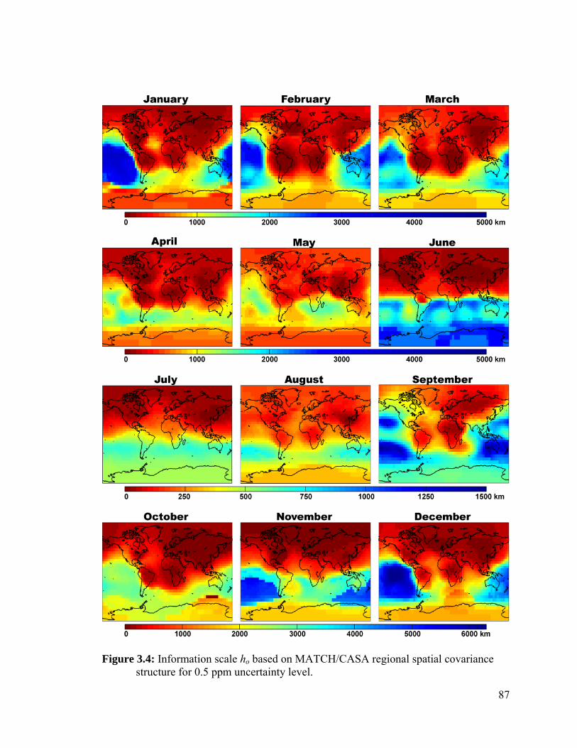
Figure 3.4: Information scale ho based on MATCH/CASA regional spatial covariance structure for 0.5 ppm uncertainty level.
87

In contrast to the NH continental regions, Australia shows large ho values that are more
affected by the SH correlation length patterns. Tropical Africa and South America show
short ho values, which reflect continental fluxes for seasons when the tropics have high
variances relative to surrounding regions. During other seasons, ho values are strongly
affected by the location of the ITCZ, with longer ho values south of the ITCZ.
Oceanic ho varies greatly between ocean basins, as well as seasonally. The Arctic Ocean
shows persistently high variability and therefore low ho, while the Southern Pacific shows
persistently lower variability and higher ho. The North and Tropical Atlantic Oceans
show some seasonality with low ho comparable to continental values for most of the year,
except in December when ho is much higher. On the other hand, the North Pacific Ocean
is highly seasonal with short ho values varying between values similar to continental
regions in June though August, and very long ho values in December. The Indian Ocean
has the strongest seasonality, with ho ranging between 350 km and 2,000 km during fall
and spring, dropping to very low values from July to September and increasing to much
longer values in November and December. Finally, the Southern Ocean spatial variability
does not show large seasonality, but shows a longitudinal distribution with high ho values
everywhere except between 60°W and 90°E where it shows higher spatial variability.
Although continental XCO2 variability is mainly controlled by surface fluxes, variability
over the oceans is less controlled by oceanic fluxes because the mixing and transport of
the highly variable land fluxes in the averaged CO2 column cause strong land fluxes to
control oceanic XCO2 variability near land regions. Furthermore, elevated variability is
88

particularly apparent over coastal regions that include both land and ocean influences.
Therefore, overall XCO2 variability over oceans does not reflect the variability of
underlying ocean fluxes as reported by studies such as McKinley et al. [2004]. This study
noted that the highest flux variability originates from the Pacific followed by the
Southern Ocean, and that the Atlantic exhibits the least flux variability. For the spatial
variability analysis presented in this chapter, the highest overall variability over oceanic
regions is over the Atlantic Ocean (particularly the North and Tropical), due to the
influence of fluxes from North America, Asia, and Europe. The Pacific Ocean shows
some seasonality that mostly reflects the seasonal change in the location of the ITCZ and
seasonal changes in transported fluxes from Asia, North and South America. These
characteristics also support the conclusion that land and not ocean fluxes are the primary
control on the variability of XCO2 over oceans.
In general, the ho parameter is used to merge the spatial covariance parameters presented
in sections 3.2.1 and 3.2.2 and provides a single representation of XCO2 variability.
Because this parameter can be defined for any variogram or covariance function, it also
serves as an ideal basis for comparison to other models and data presented in the
following section. The seasonality of CO2 surface fluxes and changes in global transport
cause the overall XCO2 variability over land and ocean areas itself to display significant
spatial and temporal variability; therefore indicating that the local XCO2 covariance
structure must be taken into account when evaluating the spatial representativeness of
individual soundings and the uncertainty associated with gap-filled XCO2 maps. Finally,
89

the factors controlling this variability go beyond those that control the variability in local
surface fluxes, with a strong observed influence of changes in global transport patterns.
3.3. Comparison to other models and aircraft data
This section tests the robustness of the modeled XCO2 spatial covariance structure to: (1)
changes in XCO2 introduced by differences in model setup, transport and CO2 fluxes, and
(2) differences between the spatial resolution of MATCH/CASA (5.5°) and the sampling
footprints of future satellites (e.g., 3km2 for OCO).
3.3.1. PCTM/GEOS-4 global simulation
The spatial variability of XCO2 fields modeled using PCTM/GEOS-4 are compared to
those from MATCH/CASA to examine whether a higher resolution model will predict
more XCO2 variability, and whether the use of assimilated meteorological fields will have
a substantial impact on the specific regions exhibiting high variability.
Figure 3.5 shows regional covariance parameters obtained from the PCTM/GEOS-4
model for January, April, July and October, 2002. The range of variances and correlation
lengths are very similar to those estimated using the MATCH/CASA model for all four
months, implying a relatively low sensitivity of inferred XCO2 variability to the increased
resolution of PCTM/GEOS-4. This result supports the contention that the
MATCH/CASA model is able to represent XCO2 variability that is representative of
observations taken at finer scales than the model grid. In other words, it begins to point
towards the idea that the majority of the variability in XCO2 occurs at scales that can be
captured by relatively coarse global models.
90

Figure 3.5 also shows that, for both models, the location and timing of high regional
variances correspond to areas with high variability in the surface fluxes due to either
fossil fuel emissions or biospheric activity. Nevertheless, there are differences in the
magnitude and spatial extent of high variance regions. The most prominent differences in
regional variances occur over: (1) Eastern Europe in January and October, where
MATCH/CASA indicates high variances whereas PCTM/GEOS-4 exhibits lower
variances, and (2) Asia, where MATCH/CASA indicates high variances during April and
October, while PCTM/GEOS-4 shows high variances over a larger area in January.
Although large differences are also found over tropical South America in April, the
variability observed in the PCTM/GEOS-4 simulation appears to be dependent on the
time of day.
Given the similarity of the fluxes prescribed in the two models, differences in the
observed location and timing of high variability regions are mostly attributable to
differences in mixing and transport. Nevertheless, some of the observed differences may
also be due to differences in sub-monthly variability in the fluxes imposed in
MATCH/CASA vs. PCTM-GEOS-4. These conclusions were further validated by
analyzing the spatial variability of the prescribed biospheric and fossil fuel fluxes, as well
as the spatial variability of XCO2 simulations using PCTM/GEOS-4 including only
biospheric or fossil fuel fluxes (e.g. Figure 3.6 and 3.7).
91
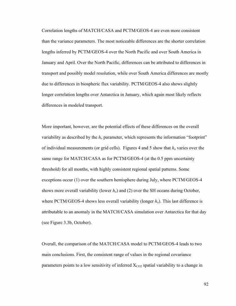
Correlation lengths of MATCH/CASA and PCTM/GEOS-4 are even more consistent
than the variance parameters. The most noticeable differences are the shorter correlation
lengths inferred by PCTM/GEOS-4 over the North Pacific and over South America in
January and April. Over the North Pacific, differences can be attributed to differences in
transport and possibly model resolution, while over South America differences are mostly
due to differences in biospheric flux variability. PCTM/GEOS-4 also shows slightly
longer correlation lengths over Antarctica in January, which again most likely reflects
differences in modeled transport.
More important, however, are the potential effects of these differences on the overall
variability as described by the ho parameter, which represents the information “footprint”
of individual measurements (or grid cells). Figures 4 and 5 show that ho varies over the
same range for MATCH/CASA as for PCTM/GEOS-4 (at the 0.5 ppm uncertainty
threshold) for all months, with highly consistent regional spatial patterns. Some
exceptions occur (1) over the southern hemisphere during July, where PCTM/GEOS-4
shows more overall variability (lower ho) and (2) over the SH oceans during October,
where PCTM/GEOS-4 shows less overall variability (longer ho). This last difference is
attributable to an anomaly in the MATCH/CASA simulation over Antarctica for that day
(see Figure 3.3b, October).
Overall, the comparison of the MATCH/CASA model to PCTM/GEOS-4 leads to two
main conclusions. First, the consistent range of values in the regional covariance
parameters points to a low sensitivity of inferred XCO2 spatial variability to a change in
92

model resolution from 5.5° × 5.5° for MATCH/CASA to 2° × 2.5° for PCTM/GEOS-4.
Second, despite some differences in the spatial patterns of the regional covariance
parameters due to differences in model winds, the overall regional spatial variability as
quantified by ho is highly consistent between the two models. These results support the
conclusion that XCO2 is a smooth process that varies on large spatial scales, and that the
spatial variability inferred from MATCH/CASA may indeed be representative of the
variability at smaller scales, as will be observed by satellites such as OCO.
93
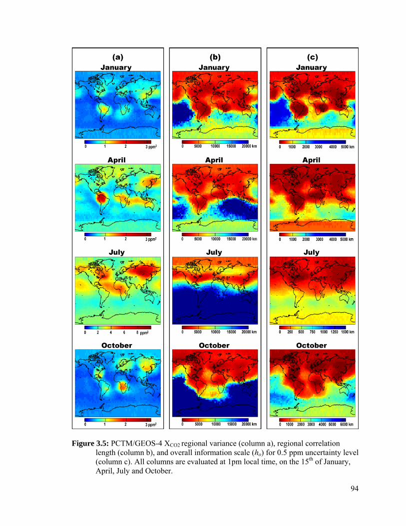
Figure 3.5: PCTM/GEOS-4 XCO2 regional variance (column a), regional correlation length (column b), and overall information scale (ho) for 0.5 ppm uncertainty level (column c). All columns are evaluated at 1pm local time, on the 15th of January, April, July and October.
94

Figure 3.6: Average total CO2 fluxes (CASA biosphere, ocean and fossil fuel) for the month of October, and its regional variance and correlation length.
(a) (b)
(c) (d)
Figure 3.7: Regional variance (a and c) and correlation length (b and d) of PCTM/GEOS-4 simulated XCO2 created by transporting: biospheric fluxes (first row), and fossil fuel fluxes (second row). PCTM/GEOS-4 XCO2 are evaluated at 1pm local time, on the 15th of October.
95
3.3.2. SiB-RAMS regional simulation
The SiB-RAMS simulation provides a measure of XCO2 spatial variability under
conditions that most closely resemble satellite measurements among the three examined
models, because: (1) the model resolution is closest to the spatial scale of future satellite
footprints, (2) the analyzed simulation represents XCO2 concentrations over North
America in August before and during the passage of a weather front, which is preceded
by large CO2 fluctuations with surface CO2 concentrations increasing by up to 40 ppm
[Wang et al., 2007], and (3) the biospheric fluxes in the SiB-RAMS simulation are
generated by the model according to the meteorological and biospheric conditions of the
simulated time period. Thus, the SiB-RAMS model represents an important validation
step for the XCO2 spatial variability that will be observed by future satellites.
Table 3.1 presents the information scale of individual measurements (or grid cells), as
represented by the parameter ho derived from the SiB-RAMS model, and compares these
values to those inferred from MATCH/CASA, PCTM/GEOS-4, and aircraft XCO2 partial
columns. The comparison shows little sensitivity of ho to the examined differences in
model resolution. For example, the average ho over North America for SiB-RAMS
simulation period is 130 km, compared to 130 km for MATCH/CASA in August. Over
the 10-day SiB-RAMS simulation, this parameter ranged from 105 km to 160 km.
Results for individual days of the SiB-RAMS simulation show that the weather front is
preceded by an increase in CO2 variability followed by a decrease during the weather
front then a return to initial variability levels of about 110 km. Even during the rapid CO2
96
fluctuations, before the passage of the weather front (between the 11th and 14th of
August), ho values do not vary substantially, indicating that although the concentrations
themselves vary in time, the scales of spatial variability remain relatively constant.
Therefore, ho values of MATCH/CASA simulations for North America can capture very
similar features in XCO2 spatial variability as a model with a 40 km resolution. Note that
a 40 km resolution is comparable to the 10 km swath width of the OCO instrument.
Although the variability of spatial processes, such as XCO2, are affected by the
measurement scale (i.e. model resolution or satellite footprint) [Gotway and Young, 2002;
Skoien and Bloschl, 2006], the PCTM/GEOS-4 and SiB-RAMS results presented in this
chapter show that model resolution within the examined range is not a major factor
controlling the spatial variability in modeled XCO2. Results of this chapter show that
XCO2 is a smooth spatial process relative to surface fluxes and concentrations. The
smoothness of XCO2 explains the low sensitivity of the inferred variability to model
resolution, and further supports the contention that the spatial variability inferred from a
relatively coarse global model can be representative of the variability that would be
observed at finer scales, and is indicative of the relative scales of variability that will need
to be captured by satellites such as OCO. This smoothness relative to surface fluxes and
concentrations is caused by the averaging of low variability CO2 at higher altitudes.
However, given that it is possible that some additional artificial smoothing is also caused
by transport effects, errors in mixing parameterization, or errors in flux distributions that
97

98
are consistent between the examined models, the spatial variabilities predicted by these
models are also compared to those derived from in-situ measurements in the next section.
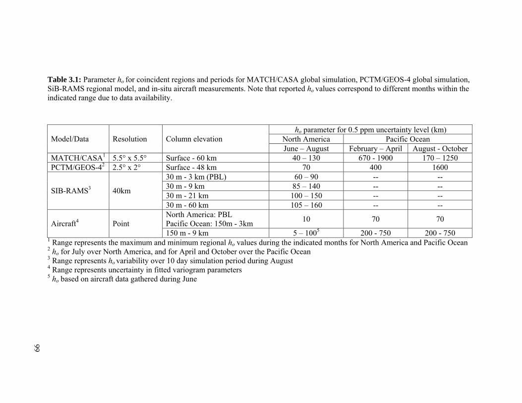
Table 3.1: Parameter ho for coincident regions and periods for MATCH/CASA global simulation, PCTM/GEOS-4 global simulation, SiB-RAMS regional model, and in-situ aircraft measurements. Note that reported ho values correspond to different months within the indicated range due to data availability.
ho parameter for 0.5 ppm uncertainty level (km) North America Pacific Ocean Model/Data Resolution Column elevation June – August February – April August - October
MATCH/CASA1 5.5° x 5.5° Surface - 60 km 40 – 130 670 - 1900 170 – 1250 PCTM/GEOS-42 2.5° x 2° Surface - 48 km 70 400 1600
30 m - 3 km (PBL) 60 – 90 -- -- 30 m - 9 km 85 – 140 -- -- 30 m - 21 km 100 – 150 -- -- SIB-RAMS3 40km
30 m - 60 km 105 – 160 -- -- North America: PBL Pacific Ocean: 150m - 3km 10 70 70 Aircraft4
1 Range represents the maximum and m hinimum regional o values during the indicated months for North America and Pacific Ocean
Point 150 m - 9 km 5 – 1005 200 - 750 200 - 750
2 ho for July over North America, and for April and October over the Pacific Ocean 3 Range represents ho variability over 10 day simulation period during August 4 Range represents uncertainty in fitted variogram parameters 5 ho based on aircraft data gathered during June
99
99

3.3.3. Aircraft data
This section compares the ho values of MATCH/CASA to the ho values calculated using
the covariance parameters of XCO2 partial columns (< 9 km) as reported in Lin et al.
[2004a]. The comparison is limited to North America and the Pacific Ocean due to the
spatial coverage of the aircraft campaigns.
For an uncertainty threshold of 0.5 ppm, the power variogram parameter ranges reported
by Lin et al., [2004a] over North America for June 2003 correspond to ho with an
uncertainty range of 5 km to 100 km. The MATCH/CASA average ho for the same month
and region is 85 km, which is within the uncertainty bounds of the parameter derived
from the aircraft data. For the Pacific Ocean (February to April and August to October
over several years), the reported covariance parameters correspond to an ho in the range
of 200 km to 750 km. The average MATCH/CASA ho for the same regions ranges from
670-1900 km and 170 - 1250 km in February – April and August – October, respectively
(Table 3.1).
In general, the spatial variability observed during the aircraft campaigns and that
predicted by MATCH/CASA are consistent over the examined regions. Differences in ho
values, particularly over the Pacific Ocean, during the sampled months can be attributed
to three factors. First, in contrast to model simulations, the aircraft data are collected on
relatively long time scales. Although Lin et al., [2004a] restricted the covariance function
calculation to data pairs within a three-hour time window, different pairs would still
100

represent multiple days or different times of the day. Therefore, non-stationary temporal
variability captured by the aircraft data may have been interpreted as additional spatial
variability. Second, XCO2 spatial variability of aircraft data is evaluated using
concentrations up to only 9 km in altitude, whereas MATCH/CASA models XCO2 up to
an elevation of 60 km, which is more comparable to the column that will be observed by
future satellites. The effect of increasing the height of the measured column on XCO2
spatial variability is demonstrated in Table 3.1, where the SiB-RAMS ho value for a 60
km column is about double its value for a 3 km column. The reduced XCO2 spatial
variability with increasing column elevation is also demonstrated by Lin et al., [2004a],
who reported variogram parameters corresponding to ho values that increase as the height
of the column increases (Table 3.1). Thus, the higher XCO2 variability observed during the
aircraft flights can also be attributed to the aircraft measurement of only partial columns
(9 km elevation), with correspondingly higher CO2 variability, relative to the column that
will be measured by OCO and that was modeled by MATCH/CASA. Third, although the
observed differences can be explained by the two factors described above, the higher
XCO2 spatial variability inferred from aircraft data relative to model simulations could
potentially also be caused by actual variability not captured by the highest resolution
model used in this chapter (SiB-RAMS) or by differences between model fluxes/transport
and actual aircraft sampling conditions. If this is the case, future satellites may observe
higher XCO2 variability than predicted by model simulations, but this last possibility
cannot be tested using the limited available data.
101
Overall, the comparison of XCO2 variability inferred from the various models and aircraft
data supports the conclusion that the scales of variability inferred using the
MATCH/CASA model are representative of those that will be observed by satellites such
as OCO. The analyses performed using PCTM/GEOS-4 and SiB-RAMS demonstrate the
robustness of the estimates described in Section 3.2 to a range of model resolutions and
setups. The comparison to aircraft data demonstrates the consistency of the estimates
with observed variability. One caveat that must be taken into account, and that cannot be
resolved given the current limited availability of column-integrated measurements, is the
remaining possibility that model simulations cannot reproduce some of the small scale
variability that will be observed by future satellites with small measurement footprints
(e.g., 3 km2 for the OCO). This is due to the high uncertainty in XCO2 spatial variability
inferred from aircraft measurements, which prevents a definite conclusion on this
question. Nevertheless, the presented results provide strong evidence that the smoothness
of the XCO2 signal means that models that would be too coarse to resolve variability in
surface CO2 concentrations may indeed be able to adequately capture variability in the
integrated XCO2 signal. In addition, the presented results demonstrate that the
predominant spatial patterns in the variability of XCO2 are consistent between models, as
well as for available field data, and that these patterns are attributable both to variability
in the underlying flux distribution, and regional and seasonal variability in global
transport.
4. Conclusions
Understanding of the spatial variability of XCO2, as well as the seasonality and regional
differences in this variability, is necessary for making optimal use of the data that will be
102
provided by satellites such as OCO. The evaluated spatial variability facilitates the use of
spatial interpolation methods to (i) gap-fill the retrieved soundings and evaluate the
uncertainty associated with gap-filled data products (ii) quantify the representation errors
associated with incorporating XCO2 into atmospheric transport models or GCMs when the
model resolution differs from the satellite footprint, and (iii) in the case of computational
limitations, design a sounding selection algorithm that captures the underlying spatial
variability of the XCO2 field.
In this chapter, the regional XCO2 spatial covariance structure is inferred using global
XCO2 distributions simulated using the MATCH/CASA model. The evaluated spatial
variability is compared to that inferred from a second higher-resolution global model, a
regional model, and aircraft measurements. Results show that the degree of observed
spatial variability is consistent among the examined models, and robust at spatial
resolutions down to 40 km. Results are also consistent with variability inferred from
aircraft measurements. Together, these results support the conclusion that the spatial
variability inferred using the MATCH/CASA model is representative of the variability of
XCO2 as will be observed at much finer footprints. Because the XCO2 signal is very
diffuse relative to surface CO2 concentrations, relatively coarse global models are able to
represent the expected degree of XCO2 spatial variability at smaller scales.
The presented analysis shows that both the variance and correlation lengths of the XCO2
field vary spatially and seasonally, and that this variability is attributable to changes in
both surface fluxes and seasonal patterns in global transport. The variance parameter
103

shows a clear cycle that reflects the NH growing season with peak values collocated with
regions of highly variable CO2 surface fluxes. The effect of transport on the variance
parameter is clearest during the NH winter months, when highly variable fluxes from NH
continents are transported to the Arctic and Northern oceans. The correlation lengths of
the XCO2 field, on the other hand, do not show a distinct seasonal cycle, but clearly reflect
transport and mixing effects. These effects are demonstrated by the contrast in
correlation lengths between the hemispheres, and the effects of the seasonal movement of
the ITCZ on the boundary between regions with low and high correlation lengths.
Overall XCO2 spatial variability is quantified using the parameter ho, which represents the
relative spatial scale of the information provided by a single XCO2 observation in a given
region. ho values vary between hemispheres and between ocean and continental regions.
Values are lowest during the NH summer over highly active continental flux areas, and
are highest over the Pacific Ocean during the NH winter. The XCO2 variability over the
oceans, particularly near continental regions, is primarily controlled by transport of CO2
signals from continental regions.
Results are consistent with the conclusion that a spatially and temporally variable
sounding density would be required to capture the regional differences in the spatial
variability of XCO2 with a uniform precision. Moreover, the representativeness of
individual soundings is expected to vary regionally and seasonally, as a function of the
heterogeneity in the identified spatial variability, with soundings from high variability
104

regions having higher representation errors when used to represent XCO2 in coarser
models.
Geophysical limitations (e.g. clouds, aerosol) and instrument characteristics (e.g. satellite
track) are expected to cause large gaps in retrieved XCO2 distributions, and computational
costs may further limit the fraction of retrieved soundings in the early parts of the OCO
mission. The evaluated XCO2 variability provides important information about the ability
of future satellites to capture the underlying XCO2 distribution given these limitations. For
example, given the maximum 2500 km coverage gap of consecutive orbits of OCO at the
equator, and discounting all other sampling limitations, this analysis suggest gap-filling
uncertainties that closely follow the patterns seen in the variance maps (Figure 3.3a),
reaching a maximum of 4 ppm over Boreal Asia in July, and with generally low values (<
1 ppm) over oceans and regions with low surface flux variability.
Finally, the analysis presented in this chapter establishes the main patterns of XCO2 spatial
variability and how surface fluxes and transport affect these patterns as simulated by
current models. Because these models reflect the current scientific understanding of
surface fluxes of CO2, the results also provide a baseline for evaluating the contribution
of future satellites in improving the present understanding of the XCO2 distribution and its
spatiotemporal variability.
105

106
CHAPTER 4
Using CO2 Spatial Variability to Quantify Representation Errors of Satellite CO2 Retrievals
1. Introduction
Satellite missions, such as the Orbiting Carbon Observatory (OCO) and the Greenhouse
Gases Observing Satellite (GOSAT), will provide global data of column-averaged CO2
dry-air mole fraction (XCO2) at high spatial resolutions. These data will be used in inverse
modeling studies to improve the precision and resolution of current estimates of global
carbon budgets [Rayner et al., 2001; Houweling et al., 2004; Chevallier et al., 2007]. The
amount of information that satellite retrievals contribute towards improving CO2 flux
estimates will depend on their error characteristics; therefore, an accurate evaluation of
the error statistics of retrieved soundings is central to providing accurate estimates of CO2
sources and sinks and their associated uncertainties [Chevallier et al. 2007; Engelen et al.
2002].
In inverse modeling studies, observation errors (a.k.a. model-data mismatch) are a
combination of: (1) measurement errors due to the satellite instrument, and any
107
approximations or errors in the retrieval algorithm, (2) transport model errors due to
modeling simplifications and the uncertainties of model parameters, (3) aggregation
errors caused by estimating CO2 fluxes at temporal and spatial resolutions coarser than
the transport model, and (4) representation errors due to the resolution mismatch between
observations and model gridcells [Enting 2002; Engelen et al, 2002; Michalak et al.
2005]. Representation errors are attributed to the inability of atmospheric transport
models to resolve the spatial and temporal variations captured by CO2 observations, due
to the low spatial and temporal resolution of the models relative to that of measurements
[Engelen et al., 2002; Gerbig et al., 2003]. In theory, the concentration value assigned to
a model gridcell should be equal to the true XCO2 mean over the area of the gridcell and
during the model time-step. In reality, the true mean is not known and is instead
estimated from the satellite retrievals. The representation error is therefore equal to the
uncertainty associated with the inferred gridcell mean, given the satellite retrievals over
the gridcell, and is a function of XCO2 variability over the sampled region. For example,
sparse retrievals over a gridcell located in a region with high XCO2 variability will be less
likely to capture the true mean for that gridcell, and will have higher representation error.
A number of studies have provided an evaluation of the representation error of
observations used in inverse modeling studies. Rödenbeck et al., [2003] approximated
representation errors using the standard deviation of simulated CO2 concentrations of
gridcells surrounding a measurement location. Although this approximation provides a
measure of simulated CO2 variability at the gridcell resolution in the region of a
measurement, it does not evaluate the representativeness of a measurement of the

108
mean CO2 concentration within a gridcell.
Van der Molen and Dolman [2007] studied the representation error of measurements of
CO2 based on model simulations. Their analysis showed that representation errors
increase with CO2 variability. The study quantified these errors empirically as the
average standard deviation of simulated CO2 fields within different radii of measurement
locations. This approach, however, requires knowledge of the entire sampled distribution
(e.g. XCO2 over gridcell) and does not evaluate the representativeness of multiple
measurements within a given gridcell.
Gerbig et al. [2003] and Lin et al. [2004] evaluated the spatial covariance of partial CO2
columns using aircraft measurements. The studies used the evaluated spatial covariance
to statistically generate simulated fields with a similar spatial covariance at small spatial
resolutions. The simulated fields were divided into subareas used to represent model
gridcells. The representation error was then evaluated as the average standard deviation
of the simulated values within each model gridcell. This evaluation reflects the variance
of the potential retrievals within a model gridcell, but does not represent the uncertainty
in estimating the gridcell mean given multiple measurements within each gridcell.
In the context of satellite data, a number of studies have evaluated the representation
error as the within-gridcell XCO2 variance (or sampling variance). Corbin et al. [2008]
and Miller et al. [2007] evaluated representation errors empirically based on high
resolution XCO2 simulations. Miller et al. [2007] sampled model gridcells according

109
to a North-South swath, and assumed that the representation error is equal to the
difference between the true simulated gridcell mean and the sample mean. Corbin et al.
[2008] extended this approach to include temporal variability and the effect of clouds, by
excluding cloudy pixels from the sampled North-South swaths. Both studies calculated
the swath means of all possible swath locations within model gridcells, and used the
statistics of the resulting swath mean distribution. Corbin et al. [2008] subtracted the
known simulated gridcell means from these distributions, and used the standard deviation
of the residuals as an estimate of the representation error. The methods presented in these
two studies cannot be reproduced for actual satellite sampling conditions, however,
because the true gridcells means are unknown.
This chapter introduces a statistical method for evaluating the representation errors
associated with using satellite retrievals to represent the mean XCO2 within atmospheric
transport model gridcells. The proposed method is based on: (1) the spatial distribution of
satellite retrievals within a model gridcell, and (2) knowledge of the degree of XCO2
variability in the vicinity of the model gridcell. The proposed method uses a geostatistical
evaluation of the XCO2 variability to quantify the spatial covariance between any two
satellite retrievals as a function of their separation distance. This spatial covariance
function can be inferred from available in situ data, XCO2 model simulations, or
potentially from the satellite retrievals themselves. Together with known retrieval
locations, the method evaluates representation errors in a way that: (1) reflects the
amount of information provided by available retrievals about the true unknown gridcell
mean, and (2) does not require knowledge of the true value of that mean. The method

110
is demonstrated using the regional spatial covariance statistics derived in chapter 3 using
modeled XCO2, together with assumed spatial distributions of satellite retrievals within
hypothetical model gridcells.
2. Data and methods
2.1. Methods
When XCO2 measurements are used as observations within a model, the XCO2 value
assigned to a given gridcell is intended to represent the true mean of the XCO2 distribution
within that gridcell. In reality, however, individual OCO XCO2 soundings will have a
much smaller footprint relative to a typical atmospheric transport model gridcell, and
these soundings will not sample the full area of gridcells. Therefore, statistically, the
representation error is the uncertainty associated with inferring the mean XCO2 for a given
gridcell using retrieved soundings. The proposed method evaluates representation errors
using block kriging [e.g. Chilès and Delfiner 1999], a spatial estimation method that uses
the spatial covariance information of XCO2 over sampled regions together with
information about the locations of retrieved soundings to quantify the uncertainty
associated with the mean XCO2 within each model gridcell (i.e. representation error σRE).
To construct the block kriging system, each model gridcell is divided into m pixels with
areas equal to the satellite sounding footprint (e.g. 3 km2 for OCO). The retrievals are
assumed to be an n×1 vector of noisy samples z taken at locations x of a random spatial
process y representing the XCO2 distribution within the gridcell at the resolution of
satellite soundings:

(1) ( ) ( )z x = y x + ε
The retrieval measurement errors (ε) have an n×n covariance matrix R, which can be
diagonal if the errors are assumed to be uncorrelated, or can have off-diagonal elements
to represent spatially-correlated retrieval errors. The XCO2 distribution within the gridcell
at the resolution of satellite soundings (y) is assumed to have a mean E[y] = Xβ, where X
is a matrix of covariate values at the sampling locations, β is a vector of coefficients, and
E[.] is the expectation operator. For the current application, the spatial mean (E[y]) within
each gridcell is assumed constant (although it can vary between gridcells); therefore, X is
an m×1 vector of ones and β is an unknown large-scale mean. y is also described using
an m×m spatial covariance matrix Q=E[(y - Xβ) (y - Xβ)T]. Each element of the
covariance matrix (Qij) is calculated based on the regional spatial covariance and the
separation distances (hij) between the gridcell pixels. For example, for an exponential
covariance structure, the elements of Q will have the form [e.g. Chilès and Delfiner
1999]:
2 exp ijij reg
reg
hQ
Lσ
⎛ ⎞= −⎜⎜
⎝ ⎠⎟⎟ (2)
where 2regσ and Lreg represent the regional XCO2 variance and range parameter, respectively,
and where the distance beyond which the correlation between any two XCO2
measurements approaches zero (i.e. the correlation length) is 3Lreg.
111

The uncertainty associated with the estimated XCO2 distribution within a gridcell (ŷ) at the
resolution of the satellite soundings can be quantified by solving the following kriging
system:
T
TT( )
T⎡ ⎤ ⎡ ⎤+ ⎡ ⎤=⎢ ⎥ ⎢ ⎥ ⎢ ⎥⎣ ⎦⎣ ⎦ ⎣ ⎦
SQSQS R SX ΛXSX 0 Μ
(3)
where S is an n×m indicator matrix of zeros and ones, with each row of S corresponding
to a single satellite retrieval, and a one indicating the location of the sampled pixel.
Equation 3 is solved for an m×n matrix of coefficients Λ and a 1×m vector of Lagrange
multipliers Μ. The Λ’s represent the weighting that each of the n retrieved soundings
receives in estimating the XCO2 value at each of the m locations within the gridcell, and M
represents the additional uncertainty resulting from the fact that the mean of the spatial
process y is assumed unknown.
The evaluated parameters (Λ and Μ) define the m×m covariance matrix (Vŷ) of the
uncertainties of the XCO2 signal at the resolution of the retrievals within each gridcell:
(4) Ty = − +V XΜ Q - QSΛ
The representation error, which is equal to the uncertainty associated with the estimated
average (or block) XCO2 within each gridcell, is evaluated by aggregating Vŷ as:
112
113
2 (5) 2 Ty= [ ] /
RE m m mσ 1 V 1
where 1m is an m×1 vector of ones. This estimated representation error, expressed as a
variance, takes explicit account of both the spatial covariance structure of XCO2 (Q), and
the physical distribution (and redundancy) of retrievals within each gridcell.
2.2. XCO2 spatial variability
To implement the method described in section 2.1, the spatial covariance of XCO2 must be
known. This covariance can be evaluated using aircraft measurements, or potentially
satellite retrievals, in the geographic region of a gridcell. Alternately, as will be presented
in this chapter, the covariance can be approximated based on model simulations of the
global XCO2 distribution.
The spatial covariance information used in this chapter is based on chapter 3, where the
spatial variability of pressure-averaged dry-air mole fractions (XCO2) was evaluated using
simulations from the PCTM/GEOS-4 global chemistry and transport model run at a 2°
latitude by 2.5° longitude resolution [Kawa et al., 2004], as well as a second global
model, a finer resolution regional model and aircraft measurements. Chapter 3 evaluated
the spatial variability of XCO2 as modeled by PCTM/GEOS-4 by fitting the exponential
covariance parameters σ2reg and Lreg (Section 2.1) in regions surrounding each gridcell.
These parameters are used here to populate the covariance matrix (Q) as shown in
equation (2).
114
2.3. Model gridcell and sampling conditions
In addition to XCO2 variability over the sampled region, representation errors also depend
on the satellite’s retrieval footprint, the transport model resolution and the spatial
distribution of retrievals within each gridcell.
To demonstrate the proposed methodology, representation errors are quantified using
hypothetical transport models with 0.5°×0.5°, 1°×1°, and 2°×2° grid resolutions. For the
first two resolutions, representation errors are quantified for a 3 km2 retrieval footprint.
To reduce computational cost, the retrieval footprint is scaled by a factor of two (i.e. 12
km2) for the 2°×2° analysis, while keeping the same swath width of 10km. The scaling
reduced the pixel number per model gridcell (i.e. m) and the number of samples per
model gridcell (i.e. n) by a factor of 4. This reduction, however, has only a minimal effect
on the representativeness of the samples, and therefore does not affect the evaluated
representation errors.
Further, representation errors are evaluated assuming two spatial distributions of
retrievals within each model gridcell, which represent idealized and adverse sampling
conditions (Figure 4.1): gridcells are sampled assuming (1) a full North-South swath of
retrievals in the middle of each gridcell, and (2) a single satellite retrieval at the corner of
each gridcell. For illustration, the two sampling conditions are applied to all model
gridcells, even at locations that would not be sampled due to the satellite track. The
115
dimensions of the swath are representative of the sampling design of OCO (i.e. 10 km
swath width), with 8 soundings across each swath for the 0.5°×0.5° and 1°×1°
hypothetical model resolution cases, and 4 soundings across for the 2°×2° case. Each
sounding is assumed to measure 2.4 km in latitude by 1.25km in longitude for the
0.5°×0.5° and 1°×1° model resolution cases, which are the dimensions of OCO footprint
in the Nadir measuring mode, and double these dimensions in the 2°×2° case.
To analyze the effects of the factors specifically controlling representation errors, no
measurement error is included in the presented analysis (R = 0). For actual satellite
retrievals, however, an accurate evaluation of the representation errors using the proposed
method requires satellite measurement errors to be incorporated in equation 3.
Although the example used here makes specific assumptions about model setup and
satellite retrievals, the method can accommodate any transport model resolution, retrieval
footprint, and retrieval distribution.

Figure 4.1: 1°×1° model gridcell at 45° latitude discretized into 3km2 pixels representing
the resolution at the scale of satellite sounding footprints. Dark gray pixels illustrate a single 8 pixel North-South swath through the middle of the gridcell. The black pixel represents a single satellite retrieval in the corner of the gridcell.
116
117
3. Results and discussion
To demonstrate the effects of seasonal changes in XCO2 variability on representation
errors, the presented method is applied for the months of January and July for both the
swath and edge sampling described in Section 2.3. The regional spatial variability
parameters evaluated in chapter 3 range from 0.24 ppm2 to 1.3 ppm2 in January, and 1.6
ppm2 to 9 ppm2 in July. The shortest observed correlation lengths were 700 km in
January, and 1800 km in July. The corresponding representation errors are presented in
Figures 4.2 and 4.3. Results show that: (1) representation errors are high over regions
with high XCO2 variability (see Figures 3.3, 3.4, and 3.5), and (2) adverse sampling
conditions increase representation errors even over areas with low XCO2 variability.
Seasonal changes in XCO2 variability cause the location of maximum representation errors
to vary seasonally. During the Northern Hemisphere (NH) summer, high representation
errors occur over East Asia, Eastern North America and extend over the Atlantic Ocean,
due to CO2 variability caused by North American fluxes (Figure 4.3). During the NH
winter, high representation errors occur over the Tropics and East Asia (Figure 4.2).
Relatively high errors are also expected during the NH winter over Eastern North
America. Representation errors are generally low over oceans and other continental areas.
Figures 4.2 and 4.3 also demonstrate that the impact of the number of retrievals and their
distribution within a gridcell is comparable to the impact of differences in XCO2
variability. Figure 4.2a shows that for one satellite retrieval located in the corner of a
gridcell, the representation errors during the NH winter range from 0.05ppm to

118
0.5ppm for the 0.5°×0.5° grid, 0.07ppm to 0.8ppm for the 1°×1° grid and from 0.1ppm to
0.9ppm for the 2°×2° grid. During the NH summer, figure 4.3a shows that representation
errors under the same sampling conditions range from 0.1ppm to 0.6ppm for the
0.5°×0.5° grid, from 0.14ppm to 0.9ppm for the 1°×1° and from 0.2ppm to 1.2ppm for
2°×2°. For a complete satellite swath in the middle of each gridcell, Figures 4.2b and 4.3b
show that, during both the NH winter and summer, representation errors range up to
0.1ppm, 0.16ppm and 0.2 ppm for the 0.5°×0.5°, 1°×1°, and 2°×2° grids, respectively.
Results also show that representation errors are a function of gridcell area. The
representation errors increase with the decreasing model gridcell resolution. Within the
examined resolution range, the errors increase by approximately 40% for each doubling
of the grid cell areas. Although representation error values change with varying model
grid cell areas, the spatial patterns remain constant. Further, for a particular model grid
resolution, representation errors decrease for all model gridcells when moving from a
single retrieval to a complete satellite swath, but this decrease is different for cells at the
equator (large gridcell area) and for cells near the poles (small gridcell area).
In general, the presented method provides a flexible framework for accounting for the
impact of geographic differences in XCO2 variability and differences in the spatial
distributions of retrieved soundings within gridcells. As such, the results presented here
can be compared to representation errors reported in previous studies for cases involving
similar sampling conditions. For example, Miller et al., [2007] estimated the
representation error using XCO2 simulated by a regional model over North America

119
(NA), as described in Section 1. Representation errors were calculated for 1km and 16km
grid resolutions for domains of 38km and 600km, respectively. Errors were found to be
approximately 0.18 ppm for both the coarse and fine resolutions. Using a similar gridcell
retrieval distribution and similar XCO2 variability, the method presented in the current
work produces similar results (0.1ppm for 0.5°×0.5° , 0.12ppm for 1°×1°, and 0.18ppm
for 2°×2°), as shown in Figure 4.3b over NA in July for a 10 km-wide swath and 3km2
sounding footprint for the 0.5°×0.5° and 1°×1° grids, and 12km2 footprint for the 2°×2°
grid. A possible reason for the difference is the small height (7.2 km) of the XCO2 column
used in Miller et al., [2007] (i.e. higher XCO2 variability) relative to the 48 km column
used here. This comparison shows that for similar gridcell sampling conditions, region,
and time, the presented method produces similar results, with the advantage that the
actual gridcell mean need not be known to perform the analysis.
Results can also be compared to those of Corbin et al. [2008] over NA and South
America (SA) under swath sampling conditions. Corbin et al. [2008] evaluated the
representation error for two model gridcell resolutions, 1 km and 5 km, and two grid
sizes, 97 km for the fine resolution and 355 km to 450km for the coarse resolution. The
analysis presented in figures 4.2 and 4.3 is repeated for August over the same analysis
locations as Corbin et al. [2008] (i.e. NA and SA), but with edge and middle swath
sampling to resemble the analysis setup of Corbin et al. [2008]. Over NA, August
representation errors range from 0.09 ppm to 0.14 ppm for the 0.5°×0.5° grid, from 0.09
ppm to 0.19 ppm for the 1°×1° grid and from 0.13 ppm to 0.3 ppm for the 2°×2° grid.
These results are comparable to the values reported by Corbin et al., [2008] for the
120
same month (0.06 ppm for the fine grid and 0.43 ppm for the coarse grid). Over SA,
August representation errors for the 2°×2° grid have the same ranges as NA with a very
minor increase to 0.15ppm and 0.2ppm for the 0.5°×0.5° and 1°×1° grids respectively.
These values are also similar to Corbin et al. [2008] values over SA of 0.21 ppm to 0.24
ppm for the fine and coarse grids, respectively. The advantage of the current method,
however, is the ability to estimate representation errors without knowledge of all possible
swath means over a gridcell, which is required by Corbin et al. [2008] and will not be
known for real satellite retrievals.
Gerbig et al. [2003] and Lin et al. [2004] evaluated the spatial covariance of aircraft XCO2
measurements over NA and the Pacific Ocean, and used these covariances to produce
statistical realizations of XCO2 at two model gridcell resolutions (5 km and 50 km) and a
range of gridcell sizes (up to 1000 km). As discussed in Section 1, the representation
error was then assumed to equal the average standard deviation of XCO2 values within all
possible gridcells of the domain. In the case of a single retrieval per gridcell, the
uncertainty associated with the inferred gridcell mean is equivalent to the variance of
XCO2 at the retrieval resolution. Therefore, the representation errors reported by Gerbig et
al.[2003] and Lin et al. [2004] are comparable to representation errors under adverse
sampling conditions. Despite the mismatch between the sample and gridcell areas, the
representation errors reported by Gerbig et al, [2003] and Lin et al. [2004] (0.5 ppm for
NA and 0.25 ppm for the Pacific Ocean, as approximated from Figure 4.3 in Lin et al.
(2004)) are comparable to the representation errors calculated here (Figures 4.2a and
4.3a), with the advantage that the approach presented here can accommodate any

121
spatial distribution of samples within gridcells.

(a) One sounding (b) Swath
2°×2
°1°
×1°
0.5°
×0.5
°
Figure 4.2: January representation errors; (a) one sounding per gridcell, (b) one swath per gridcell.
122

(a) One sounding (b) Swath2°
×2°
1°×1
°0.
5°×0
.5°
Figure 4.3: July representation error; (a) one sounding per gridcell, (b) one swath per gridcell.
123

124
4. Conclusions
Representation errors occur due to the mismatch between the spatial footprint of XCO2
retrievals and the resolution of atmospheric transport models. The magnitude of these
errors depends on the ability of retrieved soundings to capture the true XCO2 mean within
model gridcells, which in turn depends on the number and spatial distribution of
retrievals within model gridcells and the underlying spatial variability of XCO2 over the
gridcell areas.
This chapter introduces a geostatistical method for evaluating representation errors.
Unlike previous studies, the method provides a statistical tool that quantifies grid-scale
representation errors by linking the actual spatial distribution of retrievals within each
gridcell and the regional XCO2 variability. The proposed method can evaluate errors
associated with any model resolution and any satellite sounding footprint, as well as
accounting for uncorrelated or correlated measurement errors. The XCO2 variability can
be estimated using modeled XCO2 distributions, as was presented here, or could be
inferred from actual satellite retrievals. The method does not require knowledge of the
XCO2 distribution within gridcells at the resolution of the satellite footprint.
The presented method was applied using spatial covariance information from chapter 3,
assuming a hypothetical model with 0.5°×0.5°, 1°×1°, and 2°×2° resolutions and a
sounding footprint representative of OCO soundings. Results show that representation
errors vary spatially and temporally, as a function of seasonal and geographic changes

125
in XCO2 variability, and the spatial distribution of satellite retrievals within each gridcell.
Although this chapter focused on spatial representation errors, temporal XCO2 variability
would also contribute to representation errors if retrievals taken across multiple days
were used jointly to estimate XCO2 for a given location and time. Extending the presented
method to include temporal variability will be the topic of future work.

CHAPTER 5
Gap-filling XCO2 retrievals using flexible non-stationary covariance functions
1. Introduction
A main objective of carbon cycle studies is to identify and reduce uncertainties about key
processes controlling levels of atmospheric CO2 [Denman et al., 2007]. Improved
understanding of these mechanisms on local and global scales will lead to improved
predictions of atmospheric CO2 under various climate change scenarios. Field and remote
sensing observations provide critical information for identifying processes controlling
variability, and for improving parameterizations and predictions of transport and process
models.
For carbon cycle science, the sparseness of the current CO2 measurement network and the
errors caused by atmospheric transport models represent a large part of the uncertainty
associated with current estimates of global carbon fluxes (see chapter 2 - section 2 ).
Gurney et al., [2002; 2003] and Baker et al., [2006] show that fluxes estimated using
different transport models vary widely even when other modeling assumptions are held
126

constant. Satellites, such as OCO, will provide high density coverage XCO2 data with the
potential of improving the precision and resolution of estimated global CO2 fluxes.
Nevertheless, the estimated CO2 fluxes are still expected to have large differences due to
different transport model assumptions and different a priori assumptions about flux
distributions. Therefore, data sets that are independent of transport and flux assumptions
will be critical for evaluating results from different studies.
Complete fields of global CO2 concentrations that are independent of transport models
and flux assumptions are also critical for the validation of process-based models. Process-
based models simulate CO2 fluxes using knowledge of the governing biospheric
processes and observations of relevant variables (such as vegetation cover proxies,
temperature, light intensity, wind, etc.). The performance of process-based models is
often evaluated by comparing the model-simulated CO2 to atmospheric CO2
measurements. Thus, XCO2 data that are independent of transport model assumptions will
be required for the evaluation of improvements in model performance.
Currently, the creation of complete atmospheric CO2 or XCO2 fields without the use of
transport models and estimated CO2 flux fields is not possible due to limited CO2
measurements. However, the global coverage of OCO data can provide the opportunity to
create complete fields of global XCO2 using statistical methods that are independent of
any transport or flux model assumptions. These maps and associated uncertainties will
provide a unique opportunity to evaluate the performance of different studies inferring or
simulating CO2 fluxes. In this chapter, a statistical gap-filling method is applied to
127
simulated OCO retrievals. The objective of the presented analysis is to evaluate the
ability of the proposed statistical gap-filling approach to create global gap-filled maps
using OCO data, together with an evaluation of their expected accuracy and precision.
Existing literature analyzing remote sensing data of CO2 focuses on data assimilation and
inverse modeling studies that use in-situ or remote sensing data to improve state
estimates (e.g. XCO2), and associated covariances [Tiwari et al., 2007; Chevallier et al.,
2005; Engelen et al., 2004]. The validation of the results of these studies is based on
averaged spatial and temporal remote sensing observations, or comparison with time
series of surface CO2 observations. Averaging over time and space, however, does not
provide global fields of XCO2 that honor the underlying spatial and temporal structure of
the measurements, or provide a measure of uncertainty about the underlying field. Unlike
other remote sensing data (e.g. earth surface prosperities), the loss of spatial and temporal
structure is particularly important for atmospheric trace gas species such as XCO2 due to
the strong spatial and temporal variability caused by the variable underlying CO2 fluxes
and atmospheric transport and mixing. Therefore, these evaluation methods will not be
sufficient to validate the results of data assimilation and inverse modeling studies using
OCO data.
Statistical methods used to model spatially and temporally varying processes (e.g. XCO2)
using measurements from global remote sensing observations include multi-resolution
methods [Huang and Cressie 2002; Johannesson and Cressie; 2004, 2007] and flexible
fixed rank covariance models [Nychka et al., 2002; Johannesson and Cressie 2004; Shi
128

and Cressie, 2007; Cressie and Johannesson 2008]. Results of these studies demonstrate
the possibility of modeling the covariance structure of global processes using only remote
sensing data provide an estimate of the process over gap areas caused by instrumental
limitations (e.g. satellite track), and quantify the associated gap-filling uncertainty.
Although other methods are used in geophysical literature to gap-fill data (see chapter 2 -
section 3), none of these methods provide the framework for statistical modeling of the
underlying process. The advantages of statistical modeling relative to other geophysical
gap-filling methods, particularly for global remote sensing observations, are twofold.
First, unlike most geophysical gap-filling methods, geostatistical methods provide a
complete and accurate estimation of gap-filling uncertainty that accounts for all sources
of error (e.g. measurement, sampling, estimation, etc.). Second, geostatistical gap filling
methods can model the covariance and trend of large datasets with relatively large gaps
without the approximations or the iterative methods used in geophysical gap-filling
methods (e.g. chapter 3 – section 3.2).
In this chapter a flexible statistical method for modeling global remotely sensed processes
is adapted to gap-fill simulated OCO retrievals. A similar model has previously been
applied to gap-fill ozone concentrations and aerosols optical thickness measured by the
Total Ozone Mapping Spectrometer (TOMS) aboard Nimbus-7 satellite and The Multi-
angle Imaging SpectroRadiometer (MISR) aboard Terra satellite [Johannesson and
Cressie 2008, Shi and Cressie 2007]. XCO2, however, has strong and non-homogeneous
spatial and temporal variabilities and gradients (as shown in chapter 3). Therefore, a main
129

question investigated in this chapter is whether the applied statistical model can capture
this variability within realistic uncertainty bounds given the sampling characteristics of
OCO. To achieve this objective, the gap-filling is applied using realistic simulated OCO
data, and results are analyzed to: (1) evaluate the ability of the proposed statistical model
to create gap-filled XCO2 maps that are representative of average XCO2 distributions
during one OCO repeat cycle from OCO retrievals, and (2) provide an understanding of
the quality of the inferred maps.
The statistical gap-filling method uses flexible bi-square basis functions to statistically
model the XCO2 trend and empirical covariance matrix using simulated OCO
observations. These basis functions are local and multi-resolution, and are therefore able
to capture the multiple scales of XCO2 variability (see chapter 3). The statistical model is
then used in a universal kriging setup (see chapter 2 – section 4) to optimally estimate the
XCO2 distribution over gap areas, together with the associated uncertainty.
OCO will measure the global XCO2 distribution with a 16 day repeat cycle. The satellite
data coverage for a single day is very limited, and retrievals obtained over a number of
days are therefore required to provide information about the underlying XCO2 distribution.
Therefore, the statistical gap-filling presented in this chapter infers the average XCO2
distribution over half and full repeat cycles (i.e. 8 and 16 days) with an assessment of the
estimate uncertainties. In addition to interpolation error, the inferred uncertainties provide
an estimate of the measurement and sampling errors, as well as added error due to
temporal changes in the XCO2 distribution during the analysis period.
130

The gap-filling performance is evaluated by analyzing eight test cases of possible
spatiotemporal distributions of OCO measurements. For all test cases, OCO
measurements are created using simulated XCO2 at relatively high resolution. The
measurement gaps are created to reflect the OCO track and realistic cloud and aerosol
conditions, based on available satellite measurements of these quantities. The current
OCO retrieval algorithm suggests that OCO observations can be retrieved up to a total
scattering aerosol and cloud Optical Depth (OD) of 0.1 to 0.3. Therefore, for each month,
simulated XCO2 fields are sampled using 0.1 and 0.3 cloud and aerosol OD thresholds to
represent the range of possible OCO retrieval densities and distributions. Further, to
simulate the effect of measurement errors, a random error with a standard deviation of 1.5
ppm is added to all samples, which is a realistic assumption given current analyses of the
OCO retrieval algorithm (Denis O’Brien, personal communication). The gap-filling is
applied for the period of January 17th to February 1st, and July 1st to 16th, 2003, to analyze
the effects of different XCO2 variability characteristics. Finally, to test the ability of the
proposed approach to infer the average XCO2 distribution over the sampled period with
realistic uncertainty bounds, the gap-filling is performed using samples from both half
and one OCO repeat cycle, thus resulting in a total of eight test cases, four for each
month (see Table 5.1).
131
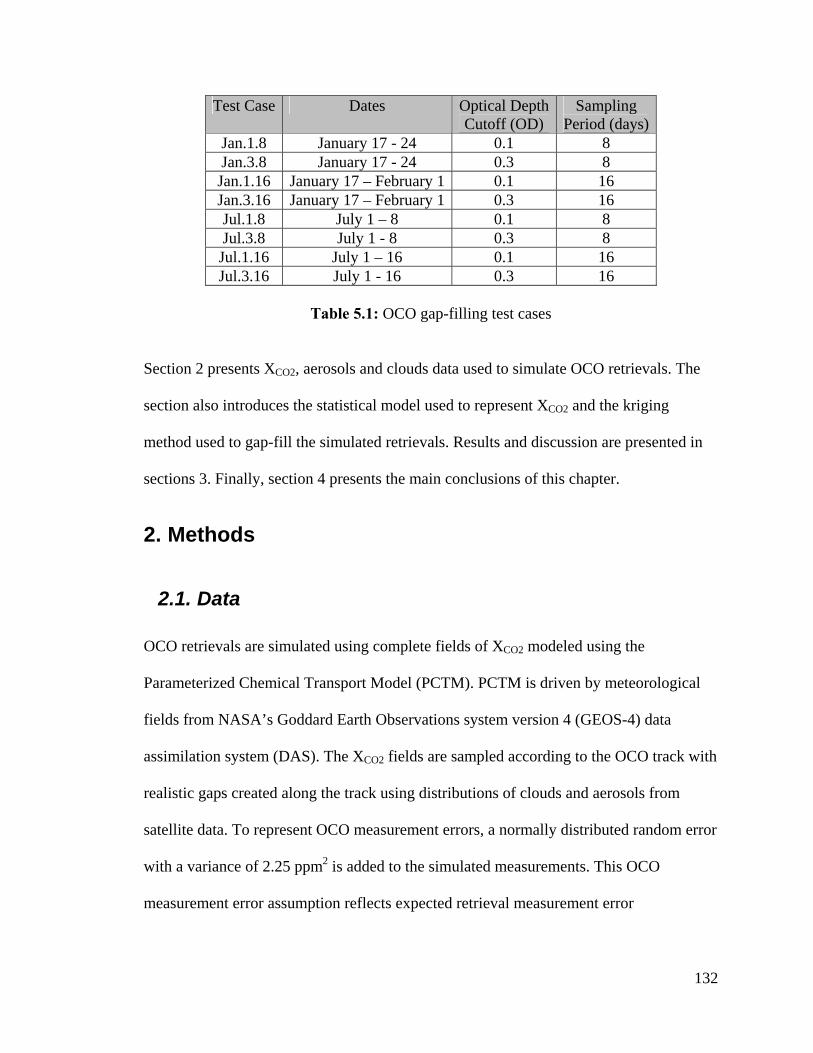
Test Case Dates Optical Depth Cutoff (OD)
Sampling Period (days)
Jan.1.8 January 17 - 24 0.1 8 Jan.3.8 January 17 - 24 0.3 8 Jan.1.16 January 17 – February 1 0.1 16 Jan.3.16 January 17 – February 1 0.3 16 Jul.1.8 July 1 – 8 0.1 8 Jul.3.8 July 1 - 8 0.3 8 Jul.1.16 July 1 – 16 0.1 16 Jul.3.16 July 1 - 16 0.3 16
Table 5.1: OCO gap-filling test cases
Section 2 presents XCO2, aerosols and clouds data used to simulate OCO retrievals. The
section also introduces the statistical model used to represent XCO2 and the kriging
method used to gap-fill the simulated retrievals. Results and discussion are presented in
sections 3. Finally, section 4 presents the main conclusions of this chapter.
2. Methods
2.1. Data
OCO retrievals are simulated using complete fields of XCO2 modeled using the
Parameterized Chemical Transport Model (PCTM). PCTM is driven by meteorological
fields from NASA’s Goddard Earth Observations system version 4 (GEOS-4) data
assimilation system (DAS). The XCO2 fields are sampled according to the OCO track with
realistic gaps created along the track using distributions of clouds and aerosols from
satellite data. To represent OCO measurement errors, a normally distributed random error
with a variance of 2.25 ppm2 is added to the simulated measurements. This OCO
measurement error assumption reflects expected retrieval measurement error
132
characteristics as estimated by current OCO retrieval algorithm tests (Denis O’Brien,
personal communication).
2.1.1. PCTM/GEOS-4
The analyzed PCTM/GEOS-4 [Kawa et al., 2004] simulation of XCO2 was run by Dr.
Randy Kawa at a 1°×1.25° horizontal resolution and a 25 layer vertical resolution
extending from the Earth surface to 48km. The model temporal resolution is hourly. The
analysis presented in this chapter is restricted to 1pm UTC to approximate the local
sampling time of OCO. To simulate XCO2, biospheric, oceanic and fossil fuel CO2
surface fluxes are transported and mixed in the atmosphere using GEOS-4 meteorological
fields for 2003.
Oceanic fluxes are based on climatological measurements of surface ocean CO2 partial
pressure [Takahashi et al., 2002]. Biospheric fluxes are based on the CASA process
model [Randerson et al., 1997] with 3-hourly resolution and zero annual mean flux at all
locations. Three-hourly flux variability is created from monthly Gross Primary
Production (GPP) and respiration using the Olsen and Randerson [2004] scaling method.
Fossil Fuel emissions are based on seasonally variable global emissions estimates by
Erickson et al., [2008].
133

2.1.2. CALIPSO clouds and aerosols
OCO measurement gaps are caused by the satellite track as well as aerosol and cloud
characteristics. Current analyses based on the OCO retrieval algorithm show that good
quality retrievals are only possible with maximum cloud and aerosol optical depth (OD)
of 0.1 to 0.3. In this work, OCO retrievals meeting this criterion are assumed successful.
The Cloud-Aerosol Lidar and Infrared Pathfinder Satellite Observation (CALIPSO) is a
recent satellite mission that provides global measurements of cloud and aerosol OD, as
well as other cloud/aerosol related variables, at relatively fine spatial resolution (the
target resolution is 5km horizontal by 60m vertical for aerosols and clouds; but the actual
resolution for aerosols can reach 40km horizontal by 120m vertical). CALIPSO is part of
the A-Train constellation, and therefore has the same track as OCO. CALIPSO OD data
for the months of January and July 2007 were obtained from the Atmospheric Science
Data Center (ASDC) – NASA Langley research center website
(http://eosweb.larc.nasa.gov/).
The Total Optical Depth (TOD) is calculated from CALIPSO optical depth layer
products. CALIPSO pixels with a sum of clouds and aerosols OD less than or equal to the
cutoff level (i.e. 0.1 or 0.3) starting from the first identified layer under the 9km elevation
to the highest identified layer are considered open. Open locations are locations where
OCO is assumed to be able to make a successful measurement.
134
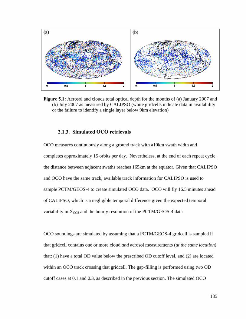
(a)
(b)
Figure 5.1: Aerosol and clouds total optical depth for the months of (a) January 2007 and
(b) July 2007 as measured by CALIPSO (white gridcells indicate data in availability or the failure to identify a single layer below 9km elevation)
2.1.3. Simulated OCO retrievals
OCO measures continuously along a ground track with a10km swath width and
completes approximately 15 orbits per day. Nevertheless, at the end of each repeat cycle,
the distance between adjacent swaths reaches 165km at the equator. Given that CALIPSO
and OCO have the same track, available track information for CALIPSO is used to
sample PCTM/GEOS-4 to create simulated OCO data. OCO will fly 16.5 minutes ahead
of CALIPSO, which is a negligible temporal difference given the expected temporal
variability in XCO2 and the hourly resolution of the PCTM/GEOS-4 data.
OCO soundings are simulated by assuming that a PCTM/GEOS-4 gridcell is sampled if
that gridcell contains one or more cloud and aerosol measurements (at the same location)
that: (1) have a total OD value below the prescribed OD cutoff level, and (2) are located
within an OCO track crossing that gridcell. The gap-filling is performed using two OD
cutoff cases at 0.1 and 0.3, as described in the previous section. The simulated OCO
135

retrievals used in the presented gap-filling analysis are limited by the resolution of
PCTM/GEOS-4 (1°×1.25° horizontal resolution), which is a much lower resolution than
that of the OCO footprint (3km2). The presented gap-filling method, however, can handle
higher data resolutions with large computational savings. Nevertheless, given the very
small footprint and the global coverage of OCO, computational limitations can still arise.
Possible extensions of the presented method to overcome such limitations include
aggregating actual OCO retrievals in space and/or time to relatively lower resolutions
using kriging methods such as block kriging (see chapter 2, section 4.5.2) to reduce
possible computational limitations, while keeping accurate error accounting.
2.2. Gap-filling
2.2.1. Statistical model
The underlying XCO2 distribution (Y(x)) is statistically modeled by assuming a spatial
mixed-effects model that consists of a large scale deterministic component μ(x), a zero
mean spatially autocorrelated stochastic component W(x), and a zero mean random
component ν(x) with a variance 2νσ that represents the part of the modeled process that is
not sampled (i.e. micro-scale variability) or not modeled (e.g. temporal variability),
2
( ) ( ) ( ) ( )(0, )N νσ
= + +Y μ W νν ∼
x x x x (1)
136

XCO2 measurements Z(x) are a noisy n×1 sample of Y(x) at measurement locations x.
The measurements Z(x) have an n×1 measurement error component (ε) assumed to be a
zero mean white noise process with a variance 2εσ ,
2
( ) ( ) ( ) ( ) ( )(0, )N εσ
= + + +Z μ W ν εε ∼
x x x x x (2)
The mean component μ(x) is modeled as a linear combination of p spatial basis functions
X that are weighted by p coefficients β (i.e. μ(x)= Xβ). The stochastic component W(x)
has a zero mean and a spatial covariance C, which is modeled using a fixed number r of
multi-resolution basis functions S [Cressie and Johannesson 2008],
(3) TC = SKS
Therefore, the complete measurement model is,
( ) = + + +Z X β S α ν εx x xx x (4)
where Xx is a known n×p matrix of trend basis functions at the measurement locations x,
and Sx is a known n×r matrix of covariance basis functions at the measurement locations
x. The trend and covariance basis functions are weighted by p×1 fixed unknown
coefficients β, and r×1 random unknown coefficients α, respectively.
From equation (4), the measurement covariance function is,
137
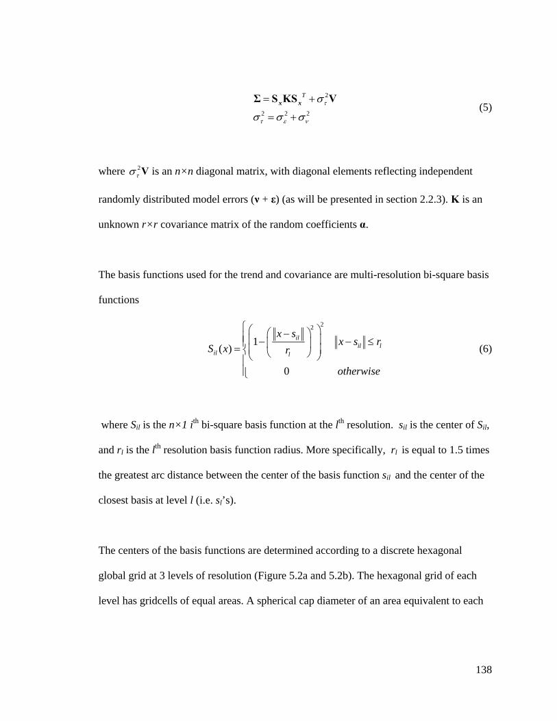
(5) 2
2 2 2
Tτ
τ ε ν
σ
σ σ σ
= +
= +
Σ S KS Vx x
where is an n×n diagonal matrix, with diagonal elements reflecting independent
randomly distributed model errors (ν + ε) (as will be presented in section 2.2.3). K is an
unknown r×r covariance matrix of the random coefficients α.
2τσ V
The basis functions used for the trend and covariance are multi-resolution bi-square basis
functions
22
1( )
0
ilil l
il l
x sx sS x r
otherwise
⎧⎛ ⎞⎛ ⎞−⎪⎜ ⎟ r− − ≤⎪ ⎜ ⎟= ⎜ ⎟⎨ ⎝ ⎠⎝ ⎠⎪⎪⎩
(6)
where Sil is the n×1 ith bi-square basis function at the lth resolution. sil is the center of Sil,
and rl is the lth resolution basis function radius. More specifically, rl is equal to 1.5 times
the greatest arc distance between the center of the basis function sil and the center of the
closest basis at level l (i.e. sl’s).
The centers of the basis functions are determined according to a discrete hexagonal
global grid at 3 levels of resolution (Figure 5.2a and 5.2b). The hexagonal grid of each
level has gridcells of equal areas. A spherical cap diameter of an area equivalent to each
138

of the levels gridcell areas are 4680km, 2700km, and 1550km for the 1st, 2nd, and 3rd
levels, respectively. The grids are generated using DGGRID software [Sahr 2001].
For the presented OCO analysis, the first level bi-square basis functions along with the
latitudinal gradient and a constant unknown component are chosen to model XCO2 trend
(i.e. the X matrix). The second and third level bi-square basis functions are used to model
the residual XCO2 covariance (i.e. the S matrix). Further, due to the non-uniform
distribution of OCO retrievals, all basis functions are tested for the possibility of empty
bases. For the various gap-filling test cases, all bases had at least 30 data points within
their area of influence.
139
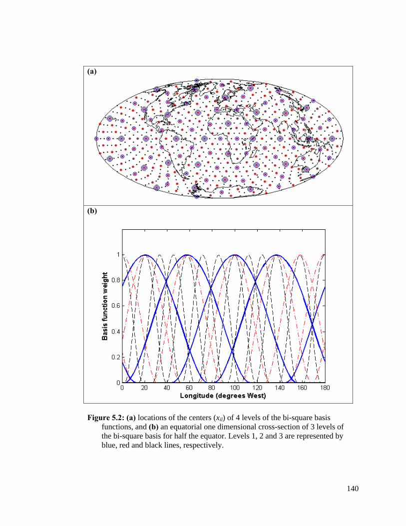
(a)
(b)
Figure 5.2: (a) locations of the centers (xil) of 4 levels of the bi-square basis
functions, and (b) an equatorial one dimensional cross-section of 3 levels of the bi-square basis for half the equator. Levels 1, 2 and 3 are represented by blue, red and black lines, respectively.
140

2.2.2. Fixed rank Kriging (FRK)
Fixed rank Kriging [Cressie and Johannesson 2008] is a type of universal kriging (see
chapter 2 – section 4.5.3) that uses a flexible fixed rank representation of the covariance
structure of the spatially structured component W(x) (equations 1 and 3). The kriging
system is constructed [Schabenberger and Gotway 2005] such that the estimated process
Ŷ(xo) is a linear combination of the data Z(x) with minimum mean squared estimation
error,
2
( ) ( )
E ( ( ) ( )) var( ( )) var( ( )) 2cov( ( ), ( ))
2o o o
o
o o
T T Tx x x
x
ox x x
=
⎡ ⎤− = + −⎣ ⎦= + −
Y aZ
aZ Y aZ Y aZ Y
aΣa S KS aS KSx
x
x x x (7)
where xo in an estimation location. Xxo is a known 1×p matrix of trend basis functions at
the estimation location xo, and Sxo is a known 1×r matrix of covariance basis functions at
the estimation location xo.
The estimator Ŷ(xo) is also constrained to be unbiased,
[ ]E ( ) ( )
0o
xo
xo
x 0− =
− =
=
aZ YaX β X βaX X
x
x
x (8)
The method of Lagrange multipliers is used to construct the objective function L, which
minimizes equation (7) subject to the unbiasness condition of equation (8),
(9) 2 2 (T T T T T Txo xo xo xo= + − + −L aΣa S KS aS KS m X a Xx x )T
Minimizing equation 9 with respect to m and a, yields the following FRK system,
141

(10) 2
0
T TTxo
Txo
τσ⎡ ⎤ ⎡⎡ ⎤+=⎢ ⎥ ⎢⎢ ⎥
⎣ ⎦⎣ ⎦ ⎣
S KS V X S KSaX Xm
x x x x
xT
⎤⎥⎦
)τσ− +V
( )
ˆxx
)T
Solving this system gives the FRK weights a,
2 1 2 1 1 2 1
2 1 1 2 1
1 1 1 1 1 1 1
( ) (1 ( ( ) ) ( )
( ( ) ) ( )
(1 ( ) ) ( )
o
o
o o
T T T T T Tx
T T T Tx
T T T T Tx x
τ τ
τ τ
σ σ
σ σ
− − −
− − −
− − − − − − −
= + − + +
+ +
= − +
a S KS S KS X X S KS X X S KS
X X S KS X X S KS
S KS X X X X X X X X
V V
V V
Σ Σ Σ Σ Σ
x x x x x x x x x x x
x x x x x x x
x x x x x x x x
(11)
Knowing that the generalized least squares estimator of the β is,
(12) 1 1 1ˆ ( )T TGLS
− − −=β X X X ZΣ Σ x
results in the FRK estimator Ŷ(xo),
(13) 1ˆˆ ( ) ( ) ( ( ) )o o
To x GLS x GLSx −= = + −Y aZ X β S KS Z X βΣxx
and the FRK estimation variance σ2K (i.e. the mean squared prediction error of Ŷ(xo)),
(14)
2
1
1 1 1 1( )( ) (
2o o o
o o o o
o o o o
T T T TK x x x
T T Tx x x x
T T T T Tx x x x
−−
− − − −+
= + −
=
− −
S KS S KS S KS
X S KS X X X X S KS X
σ a Σa S KS a S KS
Σ
Σ Σ Σ
x
x x
x x x x x x
The computational cost of inverting the very large covariance matrix Σ, however, is
prohibitive. Therefore, given the decomposition of the covariance using the fixed basis
functions (equation (5)), Cressie and Johannesson [2008] suggest using the Sherman-
Morrison-Woodbury identity,
142
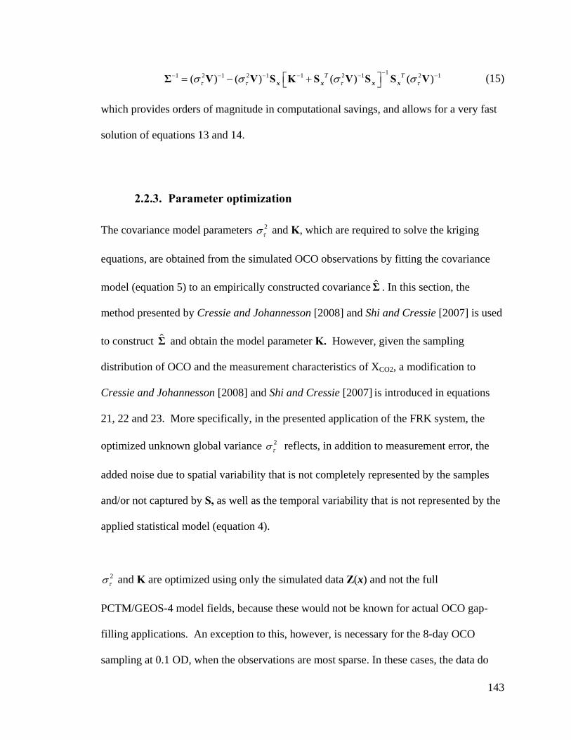
11 2 1 2 1 1 2 1 2( ) ( ) ( ) ( )T T
τ τ τ τσ σ σ σ− 1− − − − −⎡ ⎤= − +⎣ ⎦Σ V V S K S V S S Vx x x x
− (15)
which provides orders of magnitude in computational savings, and allows for a very fast
solution of equations 13 and 14.
2.2.3. Parameter optimization
The covariance model parameters 2τσ and K, which are required to solve the kriging
equations, are obtained from the simulated OCO observations by fitting the covariance
model (equation 5) to an empirically constructed covariance . In this section, the
method presented by Cressie and Johannesson [2008] and Shi and Cressie [2007] is used
to construct and obtain the model parameter K. However, given the sampling
distribution of OCO and the measurement characteristics of X
Σ
Σ
CO2, a modification to
Cressie and Johannesson [2008] and Shi and Cressie [2007] is introduced in equations
21, 22 and 23. More specifically, in the presented application of the FRK system, the
optimized unknown global variance 2τσ reflects, in addition to measurement error, the
added noise due to spatial variability that is not completely represented by the samples
and/or not captured by S, as well as the temporal variability that is not represented by the
applied statistical model (equation 4).
2τσ and K are optimized using only the simulated data Z(x) and not the full
PCTM/GEOS-4 model fields, because these would not be known for actual OCO gap-
filling applications. An exception to this, however, is necessary for the 8-day OCO
sampling at 0.1 OD, when the observations are most sparse. In these cases, the data do
143
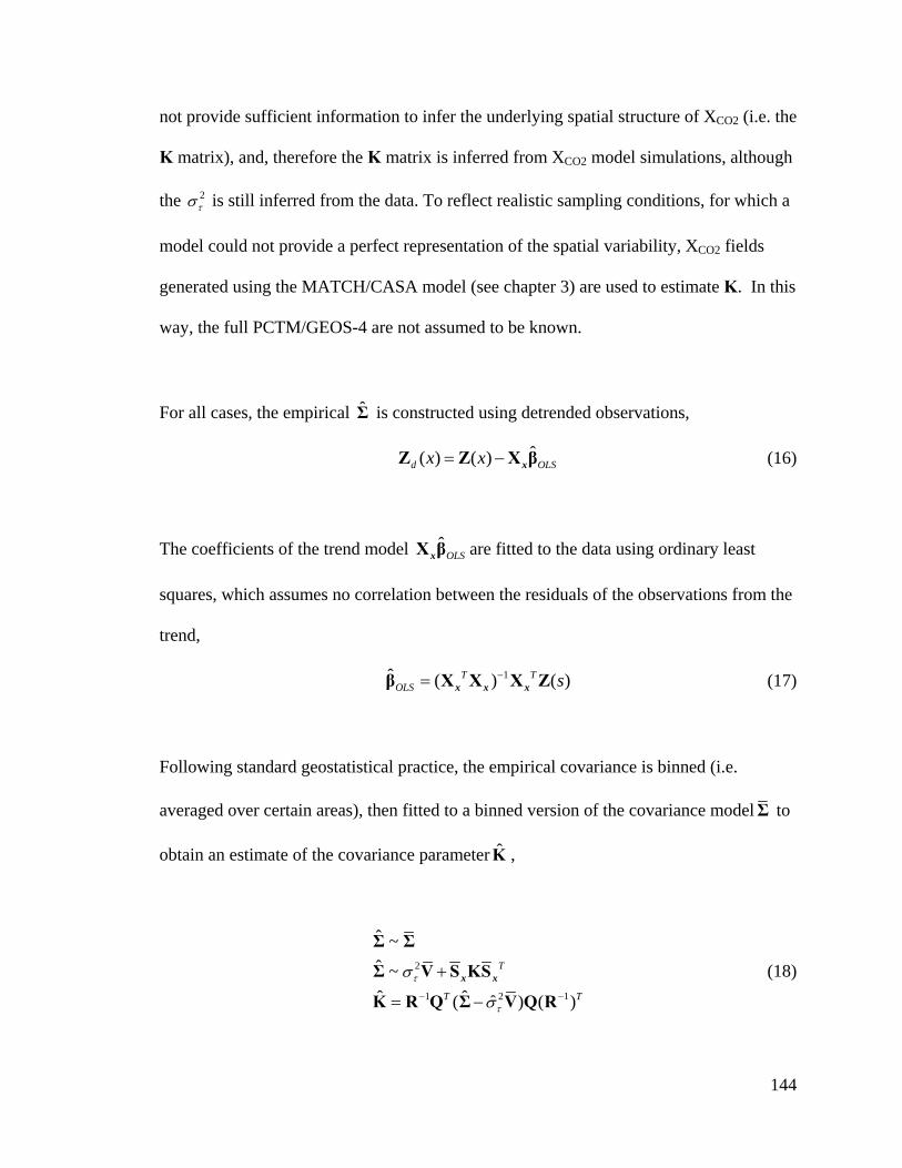
not provide sufficient information to infer the underlying spatial structure of XCO2 (i.e. the
K matrix), and, therefore the K matrix is inferred from XCO2 model simulations, although
the 2τσ is still inferred from the data. To reflect realistic sampling conditions, for which a
model could not provide a perfect representation of the spatial variability, XCO2 fields
generated using the MATCH/CASA model (see chapter 3) are used to estimate K. In this
way, the full PCTM/GEOS-4 are not assumed to be known.
For all cases, the empirical is constructed using detrended observations, Σ
(16) ˆ( ) ( )d x x= −Z Z X βx OLS
( )
The coefficients of the trend model are fitted to the data using ordinary least
squares, which assumes no correlation between the residuals of the observations from the
trend,
ˆOLSX βx
(17) 1ˆ ( )T TOLS s−=β X X X Zx x x
Following standard geostatistical practice, the empirical covariance is binned (i.e.
averaged over certain areas), then fitted to a binned version of the covariance modelΣ to
obtain an estimate of the covariance parameter , K
2
1 2ˆ
ˆ ~ˆ ~ˆ ˆ( ) (
T
T T
τ
τ
σ
σ− −
+
= −
Σ Σ
Σ V S KS
K R Q Σ V Q Rx x
1)
(18)
144

where the Q and R matrices are obtained from the QR decomposition of S x . The bins are
chosen to be circular areas centered at the locations of the 4th level of the discrete
hexagonal global grid. This grid is the same as the one used to define the centers of the
1st, 2nd and 3rd level basis functions used to model XCO2 mean and covariance. A total of
812 bins are used to construct , which is equal to the number of the 4Σ th level hexagonal
global grid centers. The bin radius is chosen to be equivalent to the resolution of the 4th
level basis function.
The best estimate of the model error parameter ( 2ˆτσ ) is obtained by minimizing the
Frobenius norm,
22 2
, ,,
ˆ ˆ ˆ( , ) (( ( ) ) ( ) )T T T Tj k j k
j kτ τσ σ− = − − −∑Σ Σ K Σ QQ Σ QQ V QQ VQQ 2 (19)
The value of 2ˆτσ that minimizes the Frobenius norm while ensuring a positive
definite is chosen. For the 8-day OCO sampling at 0.1 OD, only the inferred K 2ˆτσ is
used in the FRK system. For these cases, the K matrix is based on which is
constructed using entire MATCH/CASA X
ˆmΣ
CO2 fields,
(20) 1ˆ ˆ( ) ( )Tm
−=K R Q Σ Q R 1 T−
145

Given the current OCO retrieval algorithm, a randomly distributed measurement error
with constant unknown global variance 2εσ is a realistic assumption for OCO retrievals
(Denis O’Brien, personal communication). However, the geographically and temporally
variable XCO2 variability characteristics and the variable number of measurements within
the bins used in constructing cause variable levels of bin variances (i.e. the diagonal
elements of ). Hence, optimizing the model error parameter
Σ
Σ 2τσ by assuming =V I
would underestimate 2ˆτσ . The following weighting of the diagonal elements accounts for
these factors,
( )
, ,
, ,maxi i i space i time
iii i i space i time
VD nV
VD nγ γγ γ
∗ ∗
∗ ∗
× × ×=
× × × (21)
where VDi are the diagonal elements of the empirical matrix and nΣ i is the number of
samples in bin i. The parameters and are used to provide information about
the levels of detrended X
,i spaceγ ∗,i timeγ ∗
CO2 spatial and temporal variability within each bin (XCO2 is
detrended with respect to the trend model X). The parameter represents the
maximum squared difference between any two values of X
,i spaceγ ∗
CO2 in bin i at a particular
time within the analysis period (i.e. maximum spatial variance). To estimate , the
spatial semi-variogram of detrended X
,i spaceγ ∗
CO2 over bin i is modeled using an exponential
semi-variogram (see chapter 2, section 4). Therefore, as shown in equation 22,
occurs at the maximum possible spatial separation distance between pairs of X
,i spaceγ ∗
CO2 values
146

within bin i (hspace). Given that the bins are circular areas centered at level 4, hspace is the
diameter of bin i.
Similarly, the parameter represents the maximum squared difference between any
two values of X
,i timeγ ∗
CO2 at any particular location over bin i (i.e. maximum temporal
variance) within the analysis period. The temporal semi-variogram of detrended XCO2
over bin i is also modeled using an exponential semi-variogram. , as shown in
equation 23, occurs at the maximum possible temporal separation distance between pairs
of X
,i timeγ ∗
CO2 values within the analysis period (htime). Therefore, htime= 8 or 16days depending
on the analyzed test case,
2, ,
,
2 1 exp spacei space i space
i space
hL
γ σ∗⎛ ⎞⎛ ⎞−
= −⎜ ⎜⎜⎜ ⎝ ⎠⎝ ⎠⎟⎟⎟⎟
(22)
2, ,
,
2 1 exp timei time i time
i time
hL
γ σ∗⎛ ⎞⎛ ⎞−
= −⎜ ⎜⎜⎜ ⎝ ⎠⎝ ⎠⎟⎟⎟⎟ (23)
The parameters , and , are the spatial and temporal exponential
covariance parameters for each bin i. These parameters are derived from fitting
exponential variogram models to variogram clouds constructed using X
2,i spaceσ ,i spaceL 2
,i timeσ ,i timeL
CO2 simulated by
the MATCH/CASA model during the analysis periods (i.e. January and July).
MATCH/CASA is used here instead of PCTM/GEOS-4 to model XCO2 spatial and
temporal variability over the binned areas, such that the true XCO2 distribution
147

(represented by PCTM/GEOS-4 in this chapter) is not used to estimate the statistical
model parameters (in this case and ). This shows that the proposed method
does not depend on information that will not be available under actual OCO gap-filling
application (i.e. the true distribution of X
,i timeγ ∗,i spaceγ ∗
CO2). Given that a total of 812 bins are used to
construct , 812 sets of spatial and temporal variogram parameters are used to obtain the
and parameters for the different bins. For each bin, the variograms are fitted
using MATCH/CASA X
Σ
,i spaceγ ∗,i timeγ ∗
CO2 data within 1500 km from the bin center for 31days for each
of the two analysis periods (i.e. January and July cases).
Equation (21) allows for the optimization of the model error parameter 2τσ by
accounting for (1) the added error due to temporal XCO2 variability that is also spatially
variable over various bins (as shown in section 3), and (2) the variable sampling densities
within each bin that leads to difficulties in optimizing the measurement error and possibly
the unsampled or unmodeled small-scale spatial variability.
To provide an understanding of 2τσ caused by local temporal variability occurring during
the analysis period, exponential temporal semi-variograms are fitted to PCTM/GEOS-4
time series data during the analyzed repeat cycles for both January and July. The fitted
temporal semi-variograms provide an evaluation of XCO2 temporal variability as a
function of the temporal separation distance (htime) over PCTM/GEOS-4 gridcells. The
expected temporal variances are then estimated using the fitted parameters for each
model gridcell and the theoretical exponential semi-variogram function at htime = 8 days
and htime =16 days (Figure 5.3)
148
3. Results and discussion
Methods and data presented in the previous section are used to create synthetic data that
represent realistic OCO retrievals, and to create gap-filled XCO2 maps for the months of
January and July 2003. In this section the ability to infer the true XCO2 mean fields from
OCO data is discussed in terms of the error characteristics and estimated uncertainty of
the inferred maps. Factors affecting the quality of the maps are also explored, which
include (1) the degree of spatial and temporal variability in the underlying XCO2
distribution, and (2) the spatial distribution and density of OCO retrievals for different
time periods.
3.1. Gap-filled OCO maps
FRK is an unbiased minimum variance estimator that requires knowledge of the
covariance parameters of the estimated process (i.e. XCO2). Covariance parameter
optimization methods presented in section 2.2.3 (equations 16 - 23) are first applied to the
eight test cases of simulated OCO observations to infer, for each case, the covariance
model parameters 2τσ and K. The FRK system is then applied to infer XCO2 best estimates
(equation 13) and estimation uncertainties (equation 14) for the eight cases presented in
Table 5.1. Due to the sparse sampling for the 8-day cases at 0.1 OD, the inferred K
matrix did not provide enough information about the underlying spatial structure of XCO2.
Therefore, the K matrix for the 8-day cases at 0.1 OD is optimized using equation 20
applied to complete simulated XCO2 fields from MATCH/CASA model (see chapter 3)
for the analysis period with no measurement error. The 2τσ , on the other hand, is
optimized from the data in all test cases.
149

Figures 5.5-5.6 and 5.9-5.10 show the gap-filling results for the eight analyzed test cases,
and Table 5.2 presents summary statistics. Even for the most adverse OCO sampling
conditions (i.e. 8-day sampling with a 0.1 OD cutoff) the gap-filling method, using K
parameters inferred from MATCH/CASA model, infers the underlying XCO2 distribution
with relatively low uncertainties. Visual inspection of the inferred XCO2 fields shows that
the main features of the XCO2 distribution are reconstructed even over sparsely sampled
regions (e.g. North America (NA), South America (SA), and parts of Asia in January, and
NA and Eurasia in July). In July, however, the ability to produce a smooth map is
compromised by the particularly non-uniform geographic distribution of available
observations. The main features of the underlying “true” XCO2 field are still reproduced,
however, even over very sparsely sampled areas.
Table 5.2 shows estimates of XCO2 variability that is not represented by the basis
functions ( 2ˆτσ ) for the 8 examined cases. Values of 2ˆτσ range between 3.6ppm2 to
6.5ppm2, with the lowest value occurring for the Jan.3.8 test case. The increased values
of the inferred 2ˆτσ relative to the measurement error variance 2εσ added to the simulated
retrievals (2.25ppm2) reflect additional variability due to temporal variability or small
scale spatial variability that is not sampled by OCO and/or not fully represented by the
highest resolution levels of the multi-resolution basis functions S. The error levels
presented in Table 5.2, in addition to other factors discussed in section 3.3, are reflected
in the inferred gap-filling uncertainties.
150

More specifically, Figures 5.5-5.6 and 5.9-5.10 show that the uncertainties associated
with January gap-filled fields for the 8-day cases are generally lower than the equivalent
case for July. For 8-day OCO sampling at 0.3 OD cutoff level, the gap-filling
uncertainties are mostly within 0.4 to 0.6ppm for January and 0.4 to 0.7ppm for July.
These values increase to higher levels over regions with large gaps (e.g. parts of North
America, South America and North Africa) to reach 0.7 to 1.2ppm for both months. For
8-day gap-filling with a 0.1 OD cutoff, uncertainties over relatively large gap regions
increase to reach 0.8 to 1.5ppm for January and 1 to 1.5ppm for July. Uncertainties
associated with 16-day gap-filling and 0.3 OD cutoff for January are the lowest (within
0.5ppm for most of the globe) and increase to reach 0.4 to 0.8ppm on average at 0.1 OD,
except over limited relatively large gap areas where it can reach 1 to 1.5ppm. For July,
uncertainties range from 0.4ppm to 1ppm and can reach 1.2ppm over large gap regions.
3.2. Performance evaluation
The performance of FRK gap-filling is first evaluated using the characteristics of the
distribution of the normalized residuals. The normalized residuals are equal to the
difference between the gap-filled XCO2 field and the true XCO2 mean field for the sampled
period, normalized by the gap-filling standard deviation (i.e. gap-filling uncertainty). The
gap-filling standard deviation is the square root of the estimation variance calculated
using equation 14. In figures 5.7 and 5.11 the distributions of the residuals normalized by
the kriging standard deviation shows that, for almost all test cases, the normalized
residuals have little or no bias, and are approximately standard normal. This indicates that
the uncertainties estimated by the gap-filling approach reflect the true errors accurately,
151

and that these errors are consistent with the Gaussian assumptions inherent to the kriging
setup. Results shown in Table 5.2 demonstrate that the gap-filling uncertainties estimated
from FRK are a good representation of the uncertainty associated with the gap-filled
fields, with the truth being within +/- 2σK of the FRK best estimate 95 to 97% of the time
in all the analyzed test cases. An exception is the 16-day sampling case in July at the 0.3
OD cutoff, for which the truth is within +/- 2σK of the FRK best estimate 93% of the
time. In an ideal case scenario, 95% of true values would lie within the +/- 2σK range.
The quality of the estimated gap-filling uncertainty is further evaluated using the ratio of
the squared kriging residuals to the kriging estimation variance (SKR/ ), 2kσ
2
21
ˆ(Y( ) Y( ))1SKE /n
o o
i Ki
x xn σ=
−= ∑2
kσ (24)
Ideally, SKR/ should be equal to 1 on average. The SKR/ ratios show that the
inferred uncertainties provide a realistic representation of the gap-filling errors for all 8-
day cases and most of the 16-day cases. The SKR/ ratios for the 16-day cases during
July indicate a minor underestimation of the gap-filling uncertainties, which is consistent
with the analysis presented in the previous paragraph, although the 0.1 OD case shows
reasonable results. This underestimation is mostly caused, as described above, by the
naturally high X
2kσ
2kσ
2kσ
CO2 variability during the NH summer months together with non-uniform
OCO sampling particularly over high variability areas. During months with relatively low
spatial variability in the XCO2 signal, such as January, the characteristics of the gap-filled
152
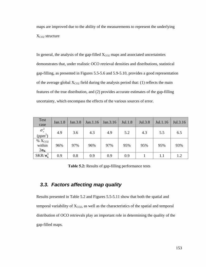
maps are improved due to the ability of the measurements to represent the underlying
XCO2 structure
In general, the analysis of the gap-filled XCO2 maps and associated uncertainties
demonstrates that, under realistic OCO retrieval densities and distributions, statistical
gap-filling, as presented in Figures 5.5-5.6 and 5.9-5.10, provides a good representation
of the average global XCO2 field during the analysis period that: (1) reflects the main
features of the true distribution, and (2) provides accurate estimates of the gap-filling
uncertainty, which encompass the effects of the various sources of error.
Test case Jan.1.8 Jan.3.8 Jan.1.16 Jan.3.16 Jul.1.8 Jul.3.8 Jul.1.16 Jul.3.16
2τσ
(ppm2) 4.9 3.6 4.3 4.9 5.2 4.3 5.5 6.5
% XCO2 within 2σK
96% 97% 96% 97% 95% 95% 95% 93%
SKR/ 2kσ 0.9 0.8 0.9 0.9 0.9 1 1.1 1.2
Table 5.2: Results of gap-filling performance tests
3.3. Factors affecting map quality
Results presented in Table 5.2 and Figures 5.5-5.11 show that both the spatial and
temporal variability of XCO2, as well as the characteristics of the spatial and temporal
distribution of OCO retrievals play an important role in determining the quality of the
gap-filled maps.
153
The analyzed gap-filling cases represent different probable scenarios of OCO retrieval
densities and distributions that are collected during a 16-day repeat cycle and spread over
the entire global domain. The presented method aims to infer the average spatial XCO2
distribution despite the high spatial and temporal variability of XCO2, which will be
reflected in the OCO data collected over the analysis period. The ability to infer the
covariance parameters and to estimate the average XCO2 fields within reasonable
uncertainties are dependant on the local levels of spatial and temporal variability of XCO2.
Non-homogeneous covariances in space or time require good sampling coverage,
particularly over high variability areas. Chapter 3 provides an extensive analysis of the
levels of spatial variability and their monthly variations, hence providing an
understanding of sampling requirements between months. As discussed in chapter 3,
XCO2 local spatial variability varies greatly between regions with particularly high local
values occurring during the NH summer months.
Figure 5.3, on the other hand, shows that XCO2 temporal variances at 8 and 16-day lags
are spatially variable (i.e. non-homogeneous) with high values occurring over and
downwind from active biosphere areas, which were also associated with high spatial
variability. Moreover, for a particular month, both the levels and the spatial distribution
of high XCO2 temporal variances are similar for the 8 and 16-day cases. This indicates that
8 and 16 day gap-filling should have (1) comparable levels of 2ˆτσ due to unmodeled
temporal variability, and (2) comparable representativeness of OCO measurements of the
underlying XCO2 variability over different regions. Large differences exist in the locations
of high temporal variances, and some differences in their levels, occur between January
154
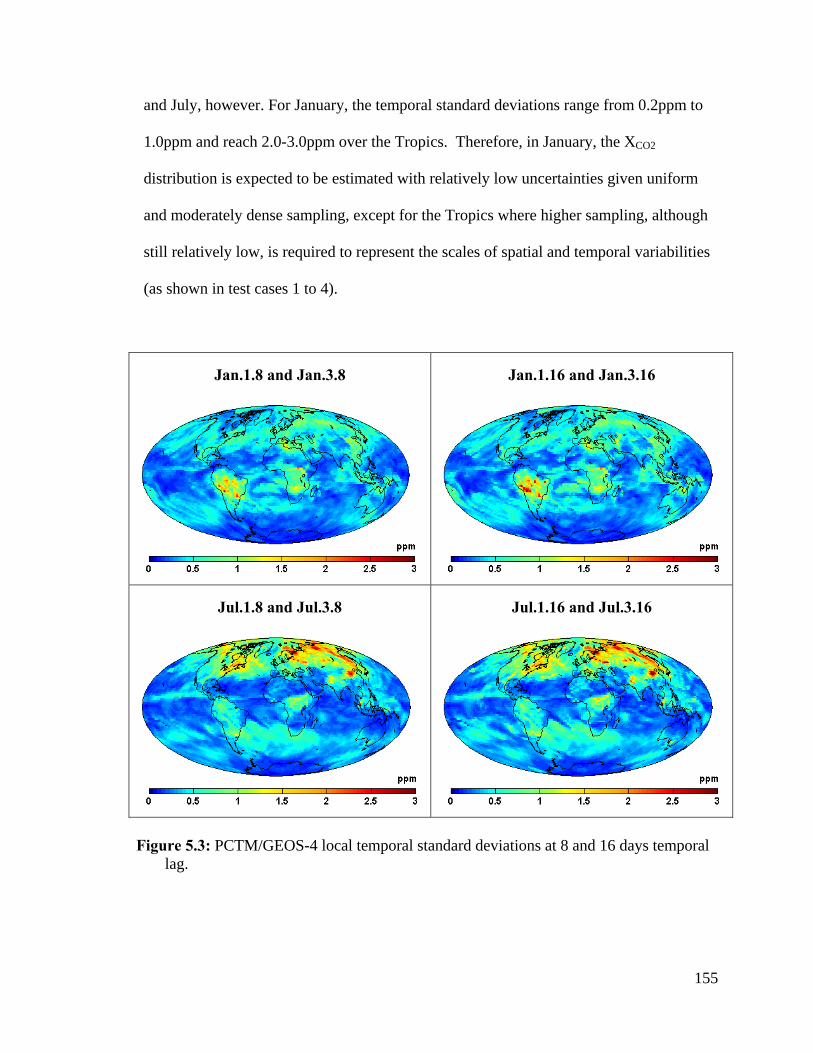
and July, however. For January, the temporal standard deviations range from 0.2ppm to
1.0ppm and reach 2.0-3.0ppm over the Tropics. Therefore, in January, the XCO2
distribution is expected to be estimated with relatively low uncertainties given uniform
and moderately dense sampling, except for the Tropics where higher sampling, although
still relatively low, is required to represent the scales of spatial and temporal variabilities
(as shown in test cases 1 to 4).
Jan.1.8 and Jan.3.8
Jan.1.16 and Jan.3.16
Jul.1.8 and Jul.3.8
Jul.1.16 and Jul.3.16
Figure 5.3: PCTM/GEOS-4 local temporal standard deviations at 8 and 16 days temporal
lag.
155

July temporal variances, on the other hand, have a larger range mostly between 0.2ppm to
2.3ppm with high variances covering large areas in the NH and reaching a maximum
value of approximately 3.0ppm. Thus, in July, the XCO2 distribution is expected to be
estimated with higher uncertainties particularly with non-uniform sampling caused by
cloud and aerosol conditions. In addition, denser sampling will be required in the NH to
represent the relatively high levels of XCO2 spatial and temporal variabilities (as shown in
July test cases).
Analysis results of the 8 test cases, Figures 5.5-5.10 and Table 5.2, reflect this non-
homogeneity of XCO2 space-time variability. Results show that the lack or sparseness of
OCO retrievals over high space/time variability areas reduces: (1) the ability of the multi-
scale covariance to represent XCO2 distribution, and (2) the ability to infer an accurate
model error parameter 2ˆτσ that captures the added error due to the scales of spatial and
temporal XCO2 variability not detected by the measurements. Although results show that
the correction given by equation (21) compensates for this under-representation of 2ˆτσ ,
still the general quality of the map and the inferred parameters is reduced due to the lack
of measurements, particularly over high variability areas.
More specifically, results show that the increase in sampling duration (e.g. 8-day vs. 16-
day sampling) causes additional temporal errors. As shown in Table 5.2, during the
month of January the inferred 2ˆτσ for the 16-day cases are about 1ppm2 higher than the
2ˆτσ for the 8-day cases with the exception of the elevated 2ˆτσ for Jan.1.8 case. This is
realistic given the relatively uniform OCO retrievals distribution and the relatively low
156

range of spatial and temporal variabilities in January. The high 2ˆτσ for the Jan.1.8 case is
mostly due to the globally sparse OCO sampling which prevents the diagonal
elements (VD
Σ
i) from capturing the actual underlying variance of XCO2 residuals. July 2ˆτσ
values for the same cases show an increase of about 2ppm2 with time and spatial
coverage. Although the inferred 2ˆτσ values for July adequately represent the gap-filling
uncertainty for most test cases, the 2ˆτσ for the Jul.3.16 case does not completely capture
the high underlying spatial and/or temporal variability as indicated by the relatively
narrow confidence intervals for the Jul.3.16 case. This underestimation is probably
caused by the non-uniform distribution of samples during July, which causes relatively
sparse sampling over regions with high underlying XCO2 variability. The non-uniform
sampling causes the high variability areas to receive less weight in the inference of 2ˆτσ
that is not completely compensated by the and parameters as presented in
equation (21).
,i spaceγ ∗,i timeγ ∗
Despite this underestimation of 2ˆτσ for the Jul.3.16 case, gap-filling results, Figures 5.5-
5.6 and 5.9-5.10, show that even under the most adverse conditions (i.e. test case Jul.1.8)
the gap-filling uncertainties are within 1.2ppm for most parts of the globe, thus indicating
that the multi-resolution covariance model applied in this chapter is able to model the
locally variable XCO2 spatial variability that is captured by OCO retrievals. In addition,
the component of the covariance model (equation 5) captures, except for Jul.3.16
case, the unstructured variability (i.e. variance component) due to measurement error, the
geographically variable X
2ˆτσ V
CO2 temporal variability (Figure 5.3), and the XCO2 spatial
157

variability at small spatial scales not captured by OCO measurements. Moreover, the
levels of gap-filling uncertainty can be greatly reduced if OCO is successful in providing
retrievals with average measurement errors less than 1.5ppm over areas equivalent to
PCTM/GEOS-4 resolution.
Results (Figures 5.5-5.10 and Table 5.2,) also show that the cloud and aerosol
distribution plays a key role in determining the quality of the gap-filled maps. Errors in
inferred maps occur mainly over sparsely sampled areas with high spatial and temporal
XCO2 variability. OCO sampling is generally extremely sparse at the 0.1 OD cutoff level,
thus preventing the possibility of inferring the K parameter from the data. In July,
Europe, Eurasia, large parts of NA, SA, and Asia are sparsely sampled. These areas have
high spatial and temporal XCO2 variability. January generally has a more uniform
distribution of samples. Nevertheless, at 0.1 OD levels, some continental areas such as
parts of Asia, NA and SA are also sparsely sampled. At 0.3 OD level, sampling of Asia
improves, however, NA and SA are still showing sparse sampling. In general, higher OD
cutoff levels provide higher densities of successful OCO retrievals. However, areas that
are sampled at 0.1 OD level are sampled even more at 0.3 OD level, while areas with
little sampling show relatively low improvement. These characteristics of OCO retrieval
distributions indicate that over particular continents the uncertainty of the gap-filled XCO2
will be generally high during winter (e.g. NA) or summer months (e.g. Asia).
158
4. Conclusions
Statistical gap-filling using synthetic datasets of OCO retrievals produces global maps of
XCO2 that approximate the true mean XCO2 distribution within reasonable gap-filling
uncertainty bounds. The gap-filling method is tested under various retrieval distribution
scenarios that reflect realistic clouds and aerosols distributions as well as the OCO track.
Results show the flexibility of the statistical model in representing the XCO2 covariance
structure, and in identifying the covariance parameters from OCO measurements.
The quality of the gap-filled maps is affected by the spatial variability of the sampled
field, the temporal variability over the sampled area, the duration of the gap-filling
period, as well as the density and spatial distribution of the samples. In general, at the 0.1
OD cutoff level, the OCO sampling is very limited and requires prior knowledge of the
spatial structure parameters K. During the NH winter months, the statistical gap-filling
shows more skill due to the more uniform OCO retrieval distribution and relatively low
XCO2 variability. Gap-filled maps during the NH summer, on the other hand, show
comparable results to winter when the sampling period is restricted to half a repeat cycle
(i.e. 8 days) due to the added temporal errors and sparse OCO sampling over high
variability NH regions. Therefore, contrary to what might be expected, extending the
estimation during NH summer to a full repeat cycle reduces the quality of both the
inferred maps and the associated uncertainties. The reduction in the quality of July maps
is due to additional OCO sampling mostly over low XCO2 variability areas, which leads to
the inference of 2ˆτσ being preferentially influenced by regions with low XCO2 variability,
while introducing limited improvement in the inferred spatial structure due to added
159

temporal errors and limited additional information about the unsampled high XCO2
variability regions.
Further, the presented gap-filling results show that global fields of XCO2 can be inferred
from OCO retrievals within uncertainty levels of 0.4 to 1ppm on average, assuming a
1.5ppm uncorrelated measurement errors over 1°×1.25° areas. Gap-filling uncertainties
can reach much higher values (approximately 1.5ppm) over limited geographical areas
with large data gaps and high underlying XCO2 variability (e.g. parts of South America
and the Northern Pacific during July).
160

(a)
(b)
Figure 5.4: Average XCO2 distribution for (a) January 17th to January 24th 2003, and
(b) January 17th to February 1st 2003
161

Test case: Jan.1.8 Test case: Jan.3.8 (a) (e)
(b) (f)
(c) (g)
(d) (h)
Figure 5.5: Gap-filling results and simulated retrievals for January 8-day test cases: (a,e)
simulated OCO samples, (b,f) gap-filled XCO2, (c,g) gap-filling uncertainty (expressed as one kriging standard deviation), (d,h) gap-filled XCO2 minus the true average modeled XCO2 over the sampled period
162
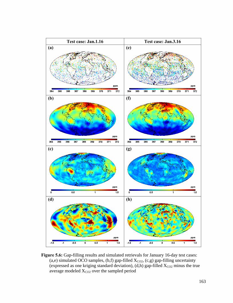
Test case: Jan.1.16 Test case: Jan.3.16 (a)
(e)
(b)
(f)
(c)
(g)
(d)
(h)
Figure 5.6: Gap-filling results and simulated retrievals for January 16-day test cases:
(a,e) simulated OCO samples, (b,f) gap-filled XCO2, (c,g) gap-filling uncertainty (expressed as one kriging standard deviation), (d,h) gap-filled XCO2 minus the true average modeled XCO2 over the sampled period
163

Figure 5.7: Distribution of normalized gap-filling residuals for January test cases
(a) Jan.1.8 (b) Jan.3.8
(c) Jan.1.16 (d) Jan.3.16
164

(a)
(b)
Figure 5.8: Average XCO2 distribution for (a) July 1st to July 8th 2003, and (b) July 1st to July 16th 2003
165

Test case: Jul.1.8 Test case: Jul.3.8
(a) (e)
(b) (f)
(c) (g)
(d) (h)
Figure 5.9: Gap-filling results and simulated retrievals for July 8-day test cases: (a,e)
simulated OCO samples, (b,f) gap-filled XCO2, (c,g) gap-filling uncertainty (expressed as one kriging standard deviation), (d,h) gap-filled XCO2 minus the true average modeled XCO2 over the sampled period
166

Test case: Jul.1.16 Test case: Jul.3.16
(a)
(e)
(b)
(f)
(c)
(g)
(d)
(h)
Figure 5.10: Gap-filling results and simulated retrievals for July 16-day test cases: (a,e)
simulated OCO samples, (b,f) gap-filled XCO2, (c,g) gap-filling uncertainty (expressed as one kriging standard deviation), (d,h) gap-filled XCO2 minus the true average modeled XCO2 over the sampled period
167

(a) Jul.1.8 (b) Jul.3.8
(c) Jul.1.16 (d) Jul.3.16
Figure 5.11: Distribution of normalized gap-filling residuals for July test cases
168

CHAPTER 6 Conclusions and Future Directions
1. Conclusions
The Objectives of this dissertation are (1) to provide a global evaluation of the regional
variability of XCO2 on monthly scales, and to use this understanding (2) to estimate
representation errors of future satellites such as OCO and, (3) to develop and implement
an effective gap-filling algorithm for the future retrievals.
In chapter 3, a global moving window semi-variogram analysis showed that the spatial
variability of model-simulated XCO2 is spatially and temporally variable. Comparing
results with another global model, a regional model, and aircraft data showed the
robustness of the estimated parameters to changes in model assumptions and resolution of
XCO2 data.
XCO2 regional variances reflect the underlying terrestrial biospheric activity. Highest
variances occur in July and August over boreal forests and the tropics, while other
regions show a fraction of these variances. During Northern Hemisphere (NH) winter, the
169
variances drop to about two thirds of their levels in the NH summer. In winter, highest
variances still reflect biospheric activity, however, effects of fossil fuel burning and
transport are also noticed.
XCO2 correlation lengths, on the other hand, show zonal patterns that reflect the limited
mixing between the northern and southern hemispheres. The NH has consistently shorter
correlations that reflect CO2 terrestrial fluxes, while the Southern Hemisphere (SH)
shows generally longer correlations that are interrupted by tropical fluxes during August
and September. Another XCO2 correlation length pattern, most likely caused by the large
scale transport of NH fluxes, is the development of short correlations in the South Pole
region during the period from December to May. The shortest South Pole correlations
(i.e. highest XCO2 variability) occur in January.
XCO2 from high resolution model simulation over North America show similar results to
the global model analysis. Comparison to the variability of aircraft measurements of
partial XCO2 columns show that for North America the results of XCO2 regional variability
analysis are within the confidence bounds of variability estimated from aircraft
measurements. For the Pacific Ocean, on the other hand, aircraft data show higher XCO2
variability, although within the range of results from the regional XCO2 variability
analysis. The increased aircraft data variability over the Pacific Ocean can be attributed to
temporal XCO2 variability due to the collection of XCO2 measurements over a number of
years, smaller XCO2 column elevation or actual variability not detected by model
170

simulations. Future analysis that compares OCO and aircraft data will further specify the
causes of this difference in variability results.
Using remote sensing data in data assimilation or inverse modeling studies requires the
quantification of the mismatch between simulated and measured remote sensing data,
caused by the difference in spatial support of the model gridcell and the satellite footprint
(i.e. representation error). Chapter 4 presented a geostatistical method to evaluate
representation errors for any satellite footprint and model gridcell resolution, given the
variability of the underlying process. Representation errors were estimated assuming
sampling conditions of OCO and hypothetical model resolutions of 0.5°×0.5°, 1°×1°, and
2°×2°. Over high variability areas, results show that XCO2 representation errors can reach
a maximum of 1.2 ppm, 0.9 ppm, and 0.6ppm for the 0.5°, 1° and 2° grid, respectively,
when a single measurement is available per model gridcell. The analysis shows that
representation errors are a function of the variability of the underlying process (i.e. XCO2),
the distribution of samples within the model gridcell, and the area of the gridcell. Areas
with high variability have higher representation errors, because a relatively large numbers
of measurements that are well-distributed within a model gridcell are required to capture
the true XCO2 mean over the gridcell area. Consequently, the location and values of
maximum XCO2 representation errors are spatially and temporally variable.
In chapter 5, synthetic OCO retrievals are used to statistically model and infer XCO2 over
expected gap areas with an evaluation of the gap-filling uncertainty. The applied
statistical model uses flexible multi-resolution basis functions to capture the spatially
171

variable XCO2 trend and covariance. Eight test cases are used to evaluate: (1) the ability of
the presented approach to infer the statistical model parameters from the retrieved data
and, (2) the performance of the gap-filling method under different sampling conditions
and underlying XCO2 variability levels. For all test cases except the most adverse case
(16-day OCO sampling at 0.3 optical depth cutoff during July), the parameters of the
statistical model were successfully inferred using the synthetic OCO data. Furthermore,
applying the proposed statistical model to gap-fill the synthetic OCO data was also
successful in producing gap-filled maps that represent the true underlying XCO2 mean
distribution within the associated gap-filling error. Results also show that the inferred
levels of gap-filling uncertainty provide an accurate representation of the various sources
of errors (e.g. temporal variability, measurement error, etc.)
Factors affecting map quality include regional levels of XCO2 spatial and temporal
variability, as well as the density and spatial distribution of available retrievals. In
January, the relatively low regional XCO2 variability and the relatively uniform global
distribution of the locations of OCO retrievals result in an improved ability to infer the
model parameters and estimate XCO2 over gap regions. The test cases also show that, for
low variability months, maps of the 8-day and 16-day mean XCO2 global fields can be
inferred within relatively low uncertainties.
On the other hand, in July, non-uniform OCO sampling, particularly the sparseness of the
samples over high XCO2 variability regions, reduces the ability to infer the true covariance
parameters. As a result, a small level of error underestimation and bias occurs in
172
estimated XCO2 fields for the 16-day July gap-filling test cases. For 8-day gap-filling, on
the other hand, July results show that XCO2 is inferred over gap regions within realistic,
but generally higher, gap-filling uncertainties relative to January. Using prior information
about the levels of variability over the sparsely sampled regions further improved the
gap-filling uncertainty estimation.
2. Future directions
The work presented in this dissertation uses covariance analysis and statistical modeling
of XCO2 distribution to develop methods for evaluating representation errors and gap-
filling of expected OCO retrievals. The presented covariance analysis reveals the non-
stationary nature of XCO2 spatial variability and its varying levels between months.
Availability of OCO data, newer aircraft observations, and FTS measurements will
provide the opportunity for expanding the covariance analysis and statistical modeling of
XCO2. In addition to XCO2 related work, future research directions also include expanding
the use of the presented geostatistical analysis to enhancing the understanding and
modeling of other environmental systems, which can greatly benefit from the increasing
information provided by remote sensing.
2.1. XCO2 covariance analysis and representation error
In chapter 3, a comparison of the regional XCO2 variability results of a number of XCO2
model simulations and aircraft data shows the robustness of XCO2 spatial variability to the
resolution and assumptions of the transport model. Nevertheless, limited data availability
allowed for relatively small coverage for aircraft measurements. Therefore, the
conclusions of chapter 3 emphasize the importance of comparing the estimated XCO2
173
variability to actual OCO retrievals and aircraft measurements that are sampled within
comparable time periods.
Objectives of future work include analyzing actual aircraft and OCO data to explore the
potential existence of undetected local variability over various regions, and evaluating its
effects on the fitted covariance parameters and representation errors. Another important
question that should be explored is whether the detected differences in the variability are
spatially and temporally consistent between years, and, if not, defining possible causes
leading to these differences and their effect on the evaluated representation errors.
Furthermore, results of chapter 3 shows that the presented spatial analysis should be
repeated to include within-month variability in the covariance structure, especially for
months corresponding to large shifts in biospheric activity (e.g. June, early July,
September, October). Therefore, another future work objective includes expanding the
analysis presented in chapter 3 to explore possible effects of joint spatiotemporal
variability.
2.2. Statistical modeling of XCO2
In chapter 5, the presented statistical gap-filling model provides the flexibility required to
represent the spatial covariance structure of XCO2 and to capture the additional errors
resulting from temporal variability within an analysis period. Tests presented in chapter 5
show the ability of the method to infer the mean XCO2 distribution over the analysis
period within gap-filling uncertainty bounds. Future work will expand the statistical
model to include the temporal evolution of XCO2, and apply the model to the much higher
174

resolution OCO data. The objective of this expansion is to explore the possibility of
developing gap-filled maps representative of shorter periods (e.g. daily instead of 8-day
or 16-day).
Possible designs for extending the method presented in chapter 5 to include statistical
modeling of the evolution of XCO2 in time and space include functional autoregressive
space-time models [Ruiz-Madina et al., 2007]. Such models, however, should be
developed to meet the characteristics of XCO2 variability and OCO observations
distribution in space and time. For example, Ruiz-Madina et al., [2007] and Salmeron
and Ruiz-Madina [2008] present an autoregressive Hilbertian model of the temporal
evolution of a system using exponential and Cauchy kernels. Theoretically, kernel
representation can semi-parametrically capture and model the evolution of the underlying
process.
2.3. Impact of presented and future work on carbon cycle
science
The main objectives of OCO mission are to improve current understanding of CO2
sources and sinks by: (1) improving the precision and resolution of current top-down
estimates of CO2 fluxes, which uses CO2 measurements, prior CO2 flux information, and
atmospheric transport models to estimate the CO2 fluxes that most probably caused the
measured CO2, and (2) improving and validating process-based models that provide
bottom-up estimates of CO2 fluxes.
175

Studies evaluating the utility of expected OCO data in improving top-down flux estimates
emphasize the need for an accurate evaluation of transport and representation errors
taking into account the spatial structure of XCO2. Such evaluation is expected to improve
the quality of inversion results [Chevallier et al., 2007b]. As explained in chapters 1 and
4, current estimates of representation errors do not reflect the underlying variability
structure of global XCO2. In chapter 3, a global analysis of XCO2 established the non-
homogeneous characteristics of XCO2 variability. The analysis presented in chapters 3 and
4, as well as the analysis proposed above, which makes use of new data, provide a
complete evaluation of the spatial and temporal variability of XCO2 as will be measured
by OCO. This evaluation and the method presented in chapter 4 provide an accurate
quantification of representation errors.
Furthermore, studies comparing top-down estimates of CO2 fluxes from different inverse
modeling studies show differences between the estimated fluxes using different transport
models [Gurney et al., 2002,2003; Baker et al., 2006a ]. Studies analyzing expected
synthetic OCO retrievals also emphasize the adverse effect of model related errors on
estimated fluxes using top-down methods [Baker et al., in press; Chevallier et al., 2007b;
Baker et al., 2006a]. The statistical gap-filling method presented in chapter 5 and the
future work suggested in section 1.2.2. provide complete fields of XCO2 that are
statistically estimated and transport model independent with associated uncertainties.
Applying these methods to actual OCO data will produce validation data sets for both
bottom-up and top-down estimates of global CO2 fluxes.
176
2.4. Using geostatistics to improve the modeling of
environmental processes
Beyond the geostatistical modeling of remotely sensed XCO2, future research directions
include extending the presented geostatistical modeling to include temporal dynamics and
multivariate analysis of other environmental systems. Such analysis would make it
possible to derive important information about the status, temporal evolution, and
controlling variables of modeled processes from field and remote sensing measurements.
In general, the availability of remote sensing data sets of many environmental variables
provides opportunities to enhance the understanding of environmental systems. In-situ
data and information about particular environmental systems are usually limited in time
and space. Remote sensing data, on the other hand, are extensive in spatial and temporal
coverage. Nevertheless, such data are also limited to a set of variables that are usually
partially informative about the underlying system. Merging the different data to provide
better understanding of the underlying system facilitates its modeling and management as
well as the design of effective monitoring schemes.
Although data assimilation methods are regularly used to incorporate data information
within physical models of studied systems, geostatistical modeling and variability
analysis provide tools for enhancing data assimilation at various scales. For example,
variability analysis (auto and cross covariances between various variables) used with
geostatistical tools such as different kriging types, Bayesian statistics, and statistical
model parameter optimization, provide valuable information that facilitates: (i) creating
177

statistical models and state estimates to explore unstudied systems or enhance existing
physical models, (ii) evaluating and incorporating scale mismatches into the process
model, and (iii) providing the framework to quantify data uncertainties and merge data
from various instruments [Wikle et al., 2001; Pardo-Iguzquiza et al., 2006 ]. Finally,
geostatistical modeling can also be extended to incorporate nonlinear functions of
ancillary variables, and therefore provide statistical modeling and parameterizations that
reflect the nature and evolution of the underlying system.
178

BIBLIOGRAPHY
179

Alkhaled, A. A., A. M. Michalak, and S. R. Kawa (2008), Using CO spatial variability to quantify representation errors of satellite CO retrievals
2
2 , Geophysical research letters, 35, L16813, doi:10.1029/2008GL034528.
Alkhaled, A. A., A. M. Michalak, S. R. Kawa, S. C. Olsen, and J.-W. Wang (2008), A
global evaluation of the regional spatial variability of column integrated CO2 distributions, Journal of Geophysical Research, 113, D20303, doi:10.1029/2007JD009693.
Alvera-Azcárate, A., A. Barth, M. Rixen, and J. M. Beckers (2005), Reconstruction of
incomplete oceanographic data sets using empirical orthogonal functions: application to the Adriatic Sea surface temperature, Ocean Modelling, 9, 325.
Alvera-Azcárate, A., A. Barth, J. M. Beckers, and R. H. Weisberg (2007), Multivariate
reconstruction of missing data in sea surface temperature, chlorophyll, and wind satellite fields, J. Geophys. Res., 112.
Andres, R. J., G. Marland, I. Fung, and E. Matthews (1996), A 1 degrees x1 degrees
distribution of carbon dioxide emissions from fossil fuel consumption and cement manufacture, 1950-1990, Global Biogeochem. Cycles, 10, 419-429.
Atkinson, P. M., and N. J. Tate (2000), Spatial scale problems and geostatistical
solutions: A review, Professional Geographer, 52, 607-623. Baker, D. F., S. C. Doney, and D. S. Schimel (2006), Variational data assimilation for
atmospheric CO2, Tellus, Ser. B, 58, 359-365. Barkley, M. P., P. S. Monks, and R. J. Engelen (2006a), Comparison of SCIAMACHY
and AIRS CO2 measurements over North America during the summer and autumn of 2003, Geophys. Res. Lett., 33, L20805, doi:20810.21029/22006GL026807.
Barkley, M. P., P. S. Monks, U. Friess, R. L. Mittermeier, H. Fast, S. Korner, and M.
Heimann (2006b), Comparisons between SCIAMACHY atmospheric CO2 retrieved using (FSI) WFM-DOAS to ground based FTIR data and the TM3 chemistry transport model, Atmos. Chem. Phys., 6, 4483-4498.
Beckers, J. M., A. Barth, and A. Alvera-Azcárate (2006), DINEOF reconstruction of
clouded images including error maps – application to the Sea-Surface Temperature around Corsican Island, Ocean Sci., 2, 183-199.
180
Beckers, J. M., and M. Rixen (2003), EOF Calculations and Data Filling from Incomplete Oceanographic Datasets, Journal of Atmospheric and Oceanic Technology, 20, 1839-1856.
Bősch, H., et al. (2006), Space-based near-infrared CO2 measurements: Testing the
Orbiting Carbon Observatory retrieval algorithm and validation concept using SCIAMACHY observations over Park Falls, Wisconsin, J. Geophys. Res., 111, D23302, doi:10.21029/22006JD007080.
Buchwitz, M., O. Schneising, J. P. Burrows, H. Bovensmann, M. Reuter, and J. Notholt
(2007), First direct observation of the atmospheric CO2 year-to-year increase from space, Atmos. Chem. Phys., 7, 5341-5342.
Buchwitz, M., et al. (2005), Carbon monoxide, methane and carbon dioxide columns
retrieved from SCIAMACHY by WFM-DOAS: year 2003 initial data set, Atmos. Chem. Phys., 5, 3313-3329.
Chahine, M. T., L. Chen, P. Dimotakis, X. Jiang, Q. B. Li, E. T. Olsen, T. Pagano, J.
Randerson, and Y. L. Yung (2008), Satellite remote sounding of mid-tropospheric CO2, Geophysical Research Letters, 35.
Chan, D., M. Ishizawa, K. Higuchi, S. Maksyutov, and J. Chen (2008), Seasonal CO2
rectifier effect and large-scale extratropical atmospheric transport, Journal of Geophysical Research-Atmospheres, 113.
Chevallier, F., F. M. Breon, and P. J. Rayner (2007), Contribution of the Orbiting Carbon
Observatory to the estimation of CO2 sources and sinks: Theoretical study in a variational data assimilation framework, J. Geophys. Res., 112, D09307, doi:10.01029/02006JD007375.
Chevallier, F., M. Fisher, P. Peylin, S. Serrar, P. Bousquet, F. M. Breon, A. Chedin, and
P. Ciais (2005), Inferring CO2 sources and sinks from satellite observations: Method and application to TOVS data, Journal of Geophysical Research-Atmospheres, 110.
Chiles, J.-P., and P. Delfiner (1999), Geostatistics: modeling spatial uncertainty, Wiley-
Interscience. Choi, Y. H., S. A. Vay, K. P. Vadrevu, A. J. Soja, J. H. Woo, S. R. Nolf, G. W. Sachse,
G. S. Diskin, D. R. Blake, N. J. Blake, H. B. Singh, M. A. Avery, A. Fried, L. Pfister, and H. E. Fuelberg (2008), Characteristics of the atmospheric CO2 signal as observed over the conterminous United States during INTEX-NA, Journal of Geophysical Research-Atmospheres, 113.
181
Conway, T. J., P. P. Tans, L. S. Waterman, and K. W. Thoning (1994), Evidence For
Interannual Variability Of The Carbon-Cycle From The National-Oceanic-And-Atmospheric-Administration Climate-Monitoring-And-Diagnostics-Laboratory Global-Air-Sampling-Network, J. Geophys. Res., 99(D11), 22,831 - 22,855.
Corbin, K. D., A. S. Denning, L. Lu, J. W. Wang, and I. T. Baker (2008), Possible
representation errors in inversions of satellite CO2 retrievals, J. Geophys. Res., 113, D02301, doi:10.01029/02007JD008716.
Cressie N., and Johannesson G. (2008), Fixed rank kriging for very large spatial data sets,
Journal of the Royal Statistical Society: Series B (Statistical Methodology), 70, 209-226.
Cressie, N. A. C. (1993), Statistics for spatial data, Revised ed., 900 pp., John Wiley &
Sons, Inc. Crisp, D., R. M. Atlas, F. M. Breon, L. R. Brown, J. P. Burrows, P. Ciais, B. J. Connor,
S. C. Doney, I. Y. Fung, D. J. Jacob, C. E. Miller, D. O'Brien, S. Pawson, J. T. Randerson, P. Rayner, R. J. Salawitch, S. P. Sander, B. Sen, G. L. Stephens, P. P. Tans, G. C. Toon, P. O. Wennberg, S. C. Wofsy, Y. L. Yung, Z. Kuang, B. Chudasama, G. Sprague, B. Weiss, R. Pollock, D. Kenyon, and S. Schroll (2004), The Orbiting Carbon Observatory (OCO) mission, Adv. Space Res., 34, 700-709.
Denman, K.L., G. Brasseur, A. Chidthaisong, P. Ciais, P.M. Cox, R.E. Dickinson, D.
Hauglustaine, C. Heinze, E. Holland, D. Jacob, U. Lohmann, S Ramachandran, P.L. da Silva Dias, S.C. Wofsy and X. Zhang, (2007), Couplings Between Changes in the Climate System and Biogeochemistry. In: Climate Change 2007: The Physical Science Basis. Contribution of Working Group I to the Fourth Assessment Report of the Intergovernmental Panel on Climate Change [Solomon, S., D. Qin, M. Manning, Z. Chen, M. Marquis, K.B. Averyt, M.Tignor and H.L. Miller (eds.)]. Cambridge University Press, Cambridge, United Kingdom and New York, NY, USA.
Denning, A. S., M. Nicholls, L. Prihodko, I. Baker, P. L. Vidale, K. Davis, and P. Bakwin
(2003), Simulated variations in atmospheric CO2 over a Wisconsin forest using a coupled ecosystem-atmosphere model, Glob. Change Biol., 9, 1241-1250, doi:10.1046/j.1365-2486.2003.00613.x.
Denning, A. S., I. Y. Fung, and D. Randall (1995), Latitudinal Gradient Of Atmospheric
Co2 Due To Seasonal Exchange With Land Biota, Nature, 376, 240-243. Denning, A. S., et al. (1999), Three-dimensional transport and concentration of SF6 - A
model intercomparison study (TransCom 2), Tellus, Ser. B, 51, 266-297.
182

Doney, S. C., D. M. Glover, S. J. McCue, and M. Fuentes (2003), Mesoscale variability
of Sea-viewing Wide Field-of-view Sensor (SeaWiFS) satellite ocean color: Global patterns and spatial scales, J. Geophys. Res., 108, 3024, doi:10.1029/2001JC000843.
Dubrule, O. (1983), Two methods with different objectives: Splines and kriging,
Mathematical Geology, 15, 245-257. Engelen, R. J., A. S. Denning, and K. R. Gurney (2002), On error estimation in
atmospheric CO2 inversions, J. Geophys. Res., 107(D22), 4635, doi: 10.1029/2002JD002195.
Engelen, R. J., E. Andersson, F. Chevallier, A. Hollingsworth, M. Matricardi, A. P.
McNally, J.-N. Thépaut, and P. D. Watts (2004), Estimating atmospheric CO from advanced infrared satellite radiances within an operational 4D-Var data assimilation system: Methodology and first results
2
, J. Geophys. Res., 109, D19309, doi:10.1029/2004JD004777.
Engelen, R. J., and A. P. McNally (2005), Estimating atmospheric CO2 from advanced
infrared satellite radiances within an operational four-dimensional variational (4D-Var) data assimilation system: Results and validation, J. Geophys. Res., 110, D18305, doi:10.1029/2005JD005982.
Enting, I. G., Inverse Problems in Atmospheric Constituent Transport, Cambridge Univ.
Press, New York, 2002. Fuentes, M. and Smith, R.L. (2001a) A New Class of Nonstationary Spatial Models.
Technical Report, North Carolina State University, Raleigh. Fuentes, M. (2001b), A high frequency kriging approach for non-stationary
environmental processes, Environmetrics, 12, 469-483. Furrer, R., and S. Sain (2008), Spatial model fitting for large datasets with applications to
climate and microarray problems, Statistics and Computing, 10.1007/s11222-11008-19075-x.
Geels, C., S. C. Doney, R. Dargaville, J. Brandt, and J. H. Christensen (2004),
Investigating the sources of synoptic variability in atmospheric CO2 measurements over the Northern Hemisphere continents: a regional model study, Tellus, Ser. B, 56, 35-50.
183

Geels, C., M. Gloor, P. Ciais, P. Bousquet, P. Peylin, A. T. Vermeulen, R. Dargaville, T. Aalto, J. Brandt, J. H. Christensen, L. M. Frohn, L. Haszpra, U. Karstens, C. Rodenbeck, M. Ramonet, G. Carboni, and R. Santaguida (2007), Comparing atmospheric transport models for future regional inversions over Europe - Part 1: mapping the atmospheric CO2 signals, Atmos. Chem. Phys., 7, 3461-3479.
Gerbig, C., J. C. Lin, S. C. Wofsy, B. C. Daube, A. E. Andrews, B. B. Stephens, P. S.
Bakwin, and C. A. Grainger (2003a), Toward constraining regional-scale fluxes of CO2 with atmospheric observations over a continent: 1. Observed spatial variability from airborne platforms, J. Geophys. Res., 108, 4756, doi:10.1029/2002JD003018.
Gerbig, C., J. C. Lin, S. C. Wofsy, B. C. Daube, A. E. Andrews, B. B. Stephens, P. S.
Bakwin, and C. A. Grainger (2003b), Toward constraining regional-scale fluxes of CO2 with atmospheric observations over a continent: 2. Analysis of COBRA data using a receptor-oriented framework, J. Geophys. Res., 108, 4757, doi:10.1029/2003JD003770.
GLOBALVIEW-CO2 (2005), Cooperative Atmospheric Data Integration Project -
Carbon Dioxide, edited, CD-ROM, NOAA CMDL, Boulder, Colorado [Also available on Internet via anonymous FTP to ftp.cmdl.noaa.gov, Path: ccg/co2/GLOBALVIEW].
Gotway, C. A., and L. J. Young (2002), Combining incompatible spatial data, J. Am. Stat.
Assoc., 97, 632-648. Gurney, K. R., R. M. Law, A. S. Denning, P. J. Rayner, D. Baker, P. Bousquet, L.
Bruhwiler, Y. H. Chen, P. Ciais, S. Fan, I. Y. Fung, M. Gloor, M. Heimann, K. Higuchi, J. John, T. Maki, S. Maksyutov, K. Masarie, P. Peylin, M. Prather, B. C. Pak, J. Randerson, J. Sarmiento, S. Taguchi, T. Takahashi, and C. W. Yuen (2002), Towards robust regional estimates of CO2 sources and sinks using atmospheric transport models, Nature, 415, 626-630.
Gurney, K. R., R. M. Law, A. S. Denning, P. J. Rayner, D. Baker, P. Bousquet, L.
Bruhwiler, Y. H. Chen, P. Ciais, S. M. Fan, I. Y. Fung, M. Gloor, M. Heimann, K. Higuchi, J. John, E. Kowalczyk, T. Maki, S. Maksyutov, P. Peylin, M. Prather, B. C. Pak, J. Sarmiento, S. Taguchi, T. Takahashi, and C. W. Yuen (2003), TransCom 3 CO2 inversion intercomparison: 1. Annual mean control results and sensitivity to transport and prior flux information, Tellus, Ser. B, 55, 555-579.
Gurney, K. R., R. M. Law, A. S. Denning, P. J. Rayner, B. C. Pak, D. Baker, P.
Bousquet, L. Bruhwiler, Y. H. Chen, P. Ciais, I. Y. Fung, M. Heimann, J. John, T. Maki, S. Maksyutov, P. Peylin, M. Prather, and S. Taguchi (2004), Transcom 3
184

inversion intercomparison: Model mean results for the estimation of seasonal carbon sources and sinks, Global Biogeochem. Cycles, 18.
Guttorp, P., and Sampson, P.D. (1994). Methods for estimating heterogeneous spatial co-
variance functions with environmental applications. In: Handbook of Statistics, 12, G.P. Patil and C.R. Rao, eds., Elsevier Science, New York, pp.661-689.
Haas, T.C. (1990), Kriging and automated variogram modeling within a moving
window, Atmospheric Environment, 24A, 1759-1769. Higdon, D. (1998). A process-convolution approach to modeling temperatures in the
North Atlantic Ocean, Journal of Environmental and Ecological Statistics, 5, 173-190.
Higdon, D.M., Swall, J., and Kern, J. (1999). Non-stationary spatial modeling. In:
Bayesian Statistics, 6, J.M. Bernardo, J.O. Berger, A.P. David, and A.F.M. Smith, eds., Oxford University Press, Oxford, 761-768.
Houweling, S., F. M. Breon, I. Aben, C. Rodenbeck, M. Gloor, M. Heimann, and P. Ciais
(2004), Inverse modeling of CO2 sources and sinks using satellite data: a synthetic inter-comparison of measurement techniques and their performance as a function of space and time, Atmos. Chem. Phys., 4, 523-538.
Huang, H.-C., Cressie, N., Gabrosek, J., (2002), Fast, resolution-consistent spatial
prediction of global processes from satellite data., J. Computnl & Graph. Statist., 11,63-88.
Isaaks, E.H. and R. M. Srivastava (1989), An introduction to applied Geostatistics,
Oxford. 1989. 561 p. Johannesson, G., N. Cressie, and H.-C. Huang (2007), Dynamic multi-resolution spatial
models, Environmental and Ecological Statistics, 14, 5. Johannesson, G., and N. Cressie (2004), Finding large-scale spatial trends in massive,
global, environmental datasets, Environmetrics, 15, 1-44. Journel, A.G., and C.J. Huijbregts (1978), Mining geostatistics, Academic Press, London. Karstens, U., M. Gloor, M. Heimann, and C. Rodenbeck (2006), Insights from
simulations with high-resolution transport and process models on sampling of the atmosphere for constraining midlatitude land carbon sinks, J. Geophys. Res., 111, D12301, doi:10.1029/2005JD006278.
185
Kawa, S. R., D. J. Erickson, S. Pawson, and Z. Zhu (2004), Global CO2 transport
simulations using meteorological data from the NASA data assimilation system, J. Geophys. Res., 109, D18312, doi:10.11029/12004JD004554.
King, A. W., Dilling L. , Zimmerman G.P., Fairman D.M. , Houghton R.A. , Marland G.
, Rose A.Z. , and W. T.J. (2007), The First State of the Carbon Cycle Report (SOCCR): The North American Carbon Budget and Implications for the Global Carbon Cycle.
Kitanidis, P. K., Generalized covariance functions associated with the Laplace equation
and their use in interpolation and inverse problems, Water Resour. Res., 35(5), 1361-1367, 1999.
Kitanidis, P. K. (1997), Introduction to Geostatistics, Applications in Hydrogeology,
Cambridge University Press. Kitanidis, P. K. (1983), Statistical Estimation of Polynomial Generalized Covariance
Functions and Hydrologic Applications, Water Resour. Res.,, 19(4), 909-921. Kolovos, A., G. Christakos, D. T. Hristopulos, and M. L. Serre (2004), Methods for
generating non-separable spatiotemporal covariance models with potential environmental applications, Advances in Water Resources, 27, 815-830.
Law, R. M., W. Peters, C. Rodenbeck, C. Aulagnier, I. Baker, D. J. Bergmann, P.
Bousquet, J. Brandt, L. Bruhwiler, P. J. Cameron-Smith, J. H. Christensen, F. Delage, A. S. Denning, S. Fan, C. Geels, S. Houweling, R. Imasu, U. Karstens, S. R. Kawa, J. Kleist, M. C. Krol, S.-J. Lin, R. Lokupitiya, T. Maki, S. Maksyutov, Y. Niwa, R. Onishi, N. Parazoo, P. K. Patra, G. Pieterse, L. Rivier, M. Satoh, S. Serrar, S. Taguchi, M. Takigawa, R. Vautard, A. Vermeulen, and Z. Zhu (in press), TransCom model simulations of hourly atmopsheric CO2: experimental overview and diurnal cycle results for 2002, Global Biogeochem. Cycles, doi:10.1029/2007GB003050.
Lin, J. C., C. Gerbig, B. C. Daube, S. C. Wofsy, A. E. Andrews, S. A. Vay, and B. E.
Anderson (2004a), An empirical analysis of the spatial variability of atmospheric CO2: Implications for inverse analyses and space-borne sensors, Geophys. Res. Lett., 31, L23104, doi:10.1029/2004GL020957.
Lin, J. C., C. Gerbig, S. C. Wofsy, A. E. Andrews, B. C. Daube, C. A. Grainger, B. B.
Stephens, P. S. Bakwin, and D. Y. Hollinger (2004b), Measuring fluxes of trace gases at regional scales by Lagrangian observations: Application to the CO2 Budget
186

and Rectification Airborne (COBRA) study, J. Geophys. Res., 109, D15304, doi:10.1029/2004JD004754.
Lu, L. X., A. S. Denning, M. A. da Silva-Dias, P. da Silva-Dias, M. Longo, S. R. Freitas,
and S. Saatchi (2005), Mesoscale circulations and atmospheric CO2 variations in the Tapajos Region, Para, Brazil, J. Geophys. Res., 110, D21102, doi:10.1029/2004JD005757.
Magnussen, S., E. Næsset, and M. A. Wulder (2007), Efficient multiresolution spatial
predictions for large data arrays, Remote Sensing of Environment, 109, 451. Mann, M. E., S. Rutherford, E. Wahl, and C. Ammann (2005), Testing the fidelity of
methods used in proxy-based reconstructions of past climate, J. Clim., 18, 4097– 4107.
Mann, M. E., and S. Rutherford (2002), Climate reconstruction using “pseudoproxies”,
Geophys. Res. Lett., 29(10), 1501, doi:10.1029/2001GL014554. McKinley, G. A., C. Rodenbeck, M. Gloor, S. Houweling, and M. Heimann (2004),
Pacific dominance to global air-sea CO2 flux variability: A novel atmospheric inversion agrees with ocean models, Geophys. Res. Lett., 31, L22308, doi:10.1029/2004GL021069.
McNeal, R. J. (1983), NASA Global Tropospheric Experiment, Eos Trans., 64, 561–562. Michalak, A. M., A. Hirsch, L. Bruhwiler, K. R. Gurney, W. Peters, and P. P. Tans
(2005), Maximum likelihood estimation of covariance parameters for Bayesian atmospheric trace gas surface flux inversions, J. Geophys. Res., 110, D24107, doi:10.1029/2005JD005970.
Miller, C. E., D. Crisp, P. L. DeCola, S. C. Olsen, J. T. Randerson, A. M. Michalak, A.
Alkhaled, P. Rayner, D. J. Jacob, P. Suntharalingam, D. B. A. Jones, A. S. Denning, M. E. Nicholls, S. C. Doney, S. Pawson, H. Boesch, B. J. Connor, I. Y. Fung, D. O'Brien, R. J. Salawitch, S. P. Sander, B. Sen, P. Tans, G. C. Toon, P. O. Wennberg, S. C. Wofsy, Y. L. Yung, and R. M. Law (2007), Precision requirements for space-based XCO2 data, J. Geophys. Res., 112, D10314, doi:10310.11029/12006JD007659.
National Institute for Environmental Studies-Japan, J. (2006), GOSAT: Greenhouse
Gases Observing SATellite, edited, National Institute for Environmental Studies, Japan, Japan.
187

Nevison, C. D., et al. (2008), Contribution of ocean, fossil fuel, land biosphere, and biomass burning carbon fluxes to seasonal and interannual variability in atmospheric CO2 - art. no. G01010, J. Geophys. Res., 113, G01010, doi:10.1029/2007JG000408.
Nicholls, M. E., A. S. Denning, L. Prihodko, P. L. Vidale, I. Baker, K. Davis, and P.
Bakwin (2004), A multiple-scale simulation of variations in atmospheric carbon dioxide using a coupled biosphere-atmospheric model, J. Geophys. Res., 109, D18117, doi:10.1029/2003JD004482.
Nychka, D., C. Wikle, and J. A. Royle (2002), Multiresolution models for nonstationary
spatial covariance functions, Statistical Modeling, 2, 315-331. Olsen, S. C., and J. T. Randerson (2004), Differences between surface and column
atmospheric CO2 and implications for carbon cycle research, J. Geophys. Res., 109, D02301, doi:10.1029/2003JD003968.
Pardo-Iguzquiza, E., M. Chica-Olmo, and P. M. Atkinson (2006), Downscaling cokriging
for image sharpening, Remote Sensing of Environment, 102, 86-98. Patterson, H. D., and R. Thompson (1971), Recovery of inter-block information when
block sizes are unequal, Biometrika, 58, 545-554. Randerson, J. T., M. V. Thompson, T. J. Conway, I. Y. Fung, and C. B. Field (1997), The
contribution of terrestrial sources and sinks to trends in the seasonal cycle of atmospheric carbon dioxide, Global Biogeochem. Cycles, 11, 535-560.
Rayner, P. J., and D. M. O'Brien (2001), The utility of remotely sensed CO2
concentration data in surface source inversions, Geophys. Res. Lett., 28, 175-178. Rödenbeck, C., S. Houweling, M. Gloor, and M. Heimann (2003), CO2 flux history 1982-
2001 inferred from atmospheric data using a global inversion of atmospheric transport, Atmos. Chem. Phys., 3, 1919-1964.
Rutherford, S., M. E. Mann, T. L. Delworth, and R. Stouffer (2003), Climate field
reconstruction under stationary and nonstationary forcing, J. Clim., 16, 462– 479. Rutherford, S., M.E. Mann, T.J. Osborn, R.S. Bradley, K.R. Briffa, M.K. Hughes, and P.
Jones (2005), Proxy-Based Northern Hemisphere Surface Temperature Reconstructions: Sensitivity to Method, Predictor Network, Target Season, and Target Domain. J. Climate, 18, 2308–2329.
188
Ruiz-Medina MD, Salmero´n R, Angulo JM (2007) Kalman filtering from POP-based diagonalization of ARH(1). Comput Stat DataAnal, 51,4994–5008.
Salmerón, R., and M. Ruiz-Medina Multi-spectral decomposition of functional
autoregressive models, Stochastic Environmental Research and Risk Assessment. Sampson, P. D., Damian, D. and Guttorp, P. (2001), Advances in modeling and inference
for environmental processes with nonstationary spatial covariance, In: GeoENV 2000: Geostatistics for Environmental Applications (Kluwer, Dordrecht), P. Monestiez, D. Allard and R. Froidvaux, eds., 17–32.
Schneider, T., (2001), Analysis of Incomplete Climate Data: Estimation of Mean Values
and Covariance Matrices and Imputation of Missing Values, J. Climate, 14, 853–871.
Schneising, O., M. Buchwitz, J. P. Burrows, H. Bovensmann, M. Reuter, J. Notholt, R.
Macatangay, and T. Warneke (2008), Three years of greenhouse gas column-averaged dry air mole fractions retrieved from satellite – Part 1: Carbon dioxide, Atmos. Chem. Phys. Discuss., 8, 5477.
Schabenberger, O., and C. Gotway (2005), Statistical methods for spatial data analysis,
Chapman & Hall/CRC. Shi, T., and N. Cressie (2007), Global statistical analysis of MISR aerosol data: a massive
data product from NASA's Terra satellite, Environmetrics, 18, 665-680. Shia, R. L., M. C. Liang, C. E. Miller, and Y. L. Yung (2006), CO2 in the upper
troposphere: Influence of stratosphere-troposphere exchange, Geophys. Res. Lett., 33.
Skoien, J. O., and G. Bloschl (2006), Scale effects in estimating the variogram and
implications for soil hydrology, Vadose Zone J., 5, 153-167. Stephens, B. B., et al. (2007), Weak northern and strong tropical land carbon uptake from
vertical profiles of atmospheric CO2, Science, 316, 1732-1735, doi:10.1126/science.1137004.
Stohl, A. (Ed.) (2004), Inter-continental Transport of Air Pollution, Springer-Verlag,
Berlin, Heidelberg.
189
Stohl, A., S. Eckhardt, C. Forster, P. James, and N. Spichtinger (2002), On the pathways and timescales of intercontinental air pollution transport, J. Geophys. Res., 107, 4684, doi:10.1029/2001JD001396.
Takahashi, T., R. H. Wanninkhof, R. A. Feely, R. F. Weiss, D. W. Chipman, N. Bates, J.
Olafsson, C. Sabine, and S. C. Sutherland (1999), Net sea-air CO2 flux over the global oceans: An improved estimate based on the sea– air pCO2 difference, paper presented at 2nd CO2 in Oceans Symposium, Cent. for Global Environ. Res. Natl. Inst. for Environ. Stud., Tsukuba, Japan.
Tiwari, Y. K., M. Gloor, R. J. Engelen, F. Chevallier, C. Rodenbeck, S. Korner, P.
Peylin, B. H. Braswell, and M. Heimann (2006), Comparing CO2 retrieved from Atmospheric Infrared Sounder with model predictions: Implications for constraining surface fluxes and lower-to-upper troposphere transport - art. no. D17106, Journal of Geophysical Research-Atmospheres, 111, 17106-17106.
Toumazou, V., and J.F. Cretaux, (2001), Using a Lanczos Eigensolver in the Computation of Empirical Orthogonal Functions. Mon. Wea. Rev., 129, 1243–1250.
Van der Molen, M. K., and A. J. Dolman (2007), Regional carbon fluxes and the effect of
topography on the variability of atmospheric CO2, J. Geophys. Res , 112, D01104, doi:10.1029/2006JD007649.
Wang, J. W., A. S. Denning, L. X. Lu, I. T. Baker, K. D. Corbin, and K. J. Davis (2007),
Observations and simulations of synoptic, regional, and local variations in atmospheric CO2, J. Geophys. Res., 112, D04108, doi:10.1029/2006JD007410.
Warneke, T., et al. (2005), Seasonal and latitudinal variations of column averaged
volume-mixing ratios of atmospheric CO2, Geophys. Res. Lett., 32, L03808, doi:10.1029/2004GL021597.
Washenfelder, R. A., et al. (2006), Carbon dioxide column abundances at the Wisconsin
Tall Tower site, J. Geophys. Res., 111, D22305, doi:10.1029/2006JD007154. Yang, Z., R. A. Washenfelder, G. Keppel-Aleks, N. Y. Krakauer, J. T. Randerson, P. P.
Tans, C. Sweeney, and P. O. Wennberg (2007), New constraints on Northern Hemisphere growing season net flux, Geophys. Res. Lett., 34, L12807, doi:10.1029/2007GL029742.
Zeng, N., A. Mariotti, and P. Wetzel (2005), Terrestrial mechanisms of interannual CO2
variability, Global Biogeochem. Cycles, 19.
190
Zhang, Z., and M. E. Mann (2005), Coupled patterns of spatiotemporal variability in Northern Hemisphere sea level pressure and conterminous U.S. drought, J. Geophys. Res., 110, D03108, doi:10.1029/2004JD004896.
Zhang, Z., M. E. Mann, and E. R. Cook (2004), Alternative methods of proxy-based
climate field reconstruction: Application to the reconstruction of summer drought over the conterminous United States back to 1700 from drought-sensitive tree ring data, Holocene, 14, 502–516.
191