Remote Sensing Imagery (Tupin/Remote Sensing Imagery) || Models and Processing of Radar Signals

Chapter 7

Models and Processing of Radar Signals

7.1. Speckle and statistics of radar imagery

7.1.1. Physical origin

The origin of the speckle effect is due to the coherent nature of radar illuminationwith the emission of polarized waves, examined in Chapter 4. This coherentillumination gives to the SAR image this granular aspect that is so uncomfortable tolook at. To explain it, let us consider a physically homogeneous surface, like a fieldof grass. Each image pixel contains a large number of elementary scatterers. All theseelementary scatterers add their contributions to the field emitted by the pixel in acoherent way (see Figure 7.1). Each scatterer presents a geometric phase shift Δϕarising from its respective range from the sensor. The total pixel response inamplitude and phase is the vectorial addition of these elementary contributions(Figure 7.1).

The resulting electromagnetic field z is thus the addition of a “large number”Ndiff of complex elementary contributions αke

jφk , with αk and φk, the amplitudeand phase of the elementary field coming from the kth scatterer, respectively, (φk isthe intrinsic phase signature of the scatterer linked to its electromagnetic propertiesincreased by the geometric term Δϕ):

z =

Ndiff

k=1

αkejφk [7.1]

Chapter written by Florence TUPIN, Jean-Marie NICOLAS and Jean-Claude SOUYRIS.

Remote Sensing Imagery, Edited by Florence Tupin, Jordi Inglada and Jean-Marie Nicolas © ISTE Ltd 2014. Published by ISTE Ltd and John Wiley & Sons, Inc.

182 Remote Sensing Imagery

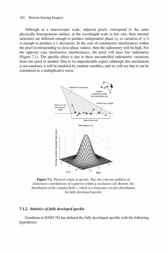
Although at a macroscopic scale, adjacent pixels correspond to the samephysically homogeneous surface, at the wavelength scale (a few cm), their internalstructures are different enough to produce independent phase φk (a variation of λ/4is enough to produce a π deviation). In the case of constructive interferences withinthe pixel (corresponding to close phase values), then the radiometry will be high. Forthe opposite case (destructive interferences), the pixel will have low radiometry(Figure 7.1). The speckle effect is due to these uncontrolled radiometric variationsfrom one pixel to another. Due to its unpredictable aspect (although this mechanismis not random), it will be modeled by random variables, and we will see that it can beconsidered as a multiplicative noise.

Figure 7.1. Physical origin of speckle. Top, the coherent addition ofelementary contributions of scatterers within a resolution cell. Bottom, the

distribution of the complex field z, which is a Gaussian circular distributionfor fully developed speckle

7.1.2. Statistics of fully developed speckle

Goodman in [GOO 76] has defined the fully developed speckle with the followinghypotheses:

Models and Processing of Radar Signals 183

1) the responses of each scatterer are independent of the others;

2) the amplitude αk and the phase φk are independent and identically distributed(in other words, all scatterers produce responses of comparable intensity; we are notconsidering here the specific case of a predominant scatterer within a cell);

3) phases φk are uniformly distributed between –π and π.

Under these hypotheses, the radiometric distribution of a uniform surface can bededuced from equation [7.1]. Based on the central limit theorem (or law of largenumbers), we obtain a circular Gaussian distribution with zero mean defined by:

p(z|σ2) = p( (z), (z)|σ2) =1

πσ2exp −|z|2

σ2[7.2]

where σ2 = E(|z|2) is connected to the backscattering coefficient of the surface,which will be called “reflectivity” from now on and denote by R. Equation [7.2] canbe obtained from the Gaussian distribution followed by the real part (z) and theimaginary part (z), with zero mean and identical standard deviation R

2 .

The equation of the probability density function (pdf) of intensity I = (z)2 +(z)2 is deduced from this:

p(I |R ) =1

Rexp (− I

R) I ≥ 0 [7.3]

This is an exponential law. Consequently, whatever the reflectivity of theconsidered region, null values are predominant. It can also be shown that the meanE(I) (moment of order 1) is equal to R:E(I) = R, and that the standard deviationσI is also equal to R. This means that the variations of the radiometric values aredirectly connected to the reflectivity of a region. The more it increases, the more theapparent heterogeneity increases. Therefore, in radar imagery, variations aremeasured by the “normalized” standard deviation called “variation coefficient” anddefined by:

CI =σI

E(I)

The value of the variation coefficient on a homogeneous region in an intensityimage is 1.

The pdf p(A |R ) of the amplitude A =√I is obtained from the relation:

p(A |R )dA = p(I |R )dI = 2p(I |R )AdA [7.4]


giving:

p (A |R ) =2A

Rexp (−A2

R) A ≥ 0 [7.5]

The amplitude of the image is distributed according to a Rayleigh law1, with a

mean E(A) = Rπ4 and with the standard deviation σA = R(1− π

4 ). Thevariation coefficient CA is approximately 0.523 for a homogeneous area of anamplitude image. Again, when E(A) increases, σA increases proportionally. Thismeans that the variations of the gray levels of a region increase with its reflectivity.Thus, the areas with strong radiometries appear “noisier” than the dark areas.

In opposition to the data that we will see in the following section 7.1.3, the imagesI = |z|2 and A = |z| are called single-look data.

7.1.3. Speckle noise in multi-look images

The speckle effect strongly limits the understanding of radar images. Therefore,multi-look images are generated to improve the radiometric resolution of radarsignals. The generation of multi-look images is based on incoherent sums ofsingle-look images. Multi-look images are generally built on the basis of intensityimages: the L-look intensity image is obtained by averaging L uncorrelated 1-lookintensity images. These L images are obtained by dividing the radar syntheticaperture into L sub-apertures. Each sub-aperture creates an uncorrelated image.However, the resolution worsens (multiplication by L). Done in the spatial field, themulti-look operation associates a unique pixel with any batch of na azimuth pixeland nd range pixels:

IL =1

nand

nand

k=1

Ik [7.6]

where Ik is the intensity of the kth pixel. The number of looks is given by L=na nd,if spatial correlation between nearby pixels is ignored. Yet, spatial correlation does

1 According to equation [7.3] the probability density of I reaches its maximum in 0, whereasaccording to [7.5], the probability density of A =

√I is null in 0! This apparent paradox

reminds us that we must not mistake the probability density with a probability. The differentialform [7.4] ensures the equality of the probabilities connected to the events A = a and I = a2.


occur, as the radar signal is always over-sampled to some extent. The intensityvariation coefficient of the multi-look image is given by:

CIL =var(IL)

E(IL)=

(var(Ik)/L)

E (Ik)= CI/

√L = 1/

√L [7.7]

The decrease in the variation coefficient of a factor√L expresses the amount of

speckle reduction.

If we do this multi-look averaging starting from an intensity image that verifiesan exponential law (equation [7.3]), then the multi-look image follows a generalizedGamma law (denoting by Γ the Gamma function):

pL(I|R) =LL

RLΓ(L)I(L−1)e(−

LIR ) [7.8]

To build the multi-look amplitude images, two techniques are available:

– calculating a multi-look intensity image and taking the square root: this is whatwe call the image

√I;

– doing the image average in amplitude: this is a classic operation in imageprocessing, which guarantees certain properties of linearity, among others.

In the first case (image√I), we can analytically calculate the pdf because the pdf

is known for the “L-looks” intensity images: we then obtain the Rayleigh-Nakagamilaw:

pL(A|R) =2LL

RLΓ(L)A(2L−1)e

−LA2

R [7.9]

In the second case, the probability law does not have a simple analytical equationand needs several approximations.

It is important to note that these types of laws (Rayleigh-Nakagami for theamplitude images, generalized Gamma law for the intensity images) are defined inIR+ and therefore have specific characteristics: in particular, the R parameter, theaverage (order 1 moment) and the mode (a value corresponding to the law’smaximum) are not equal, contrary to the Gaussian case. As we have seen, in themulti-look case with an L factor, the variation coefficients take on the values 1√

Lin

intensity and around 0.5√L

in amplitude for a physically homogeneous area.

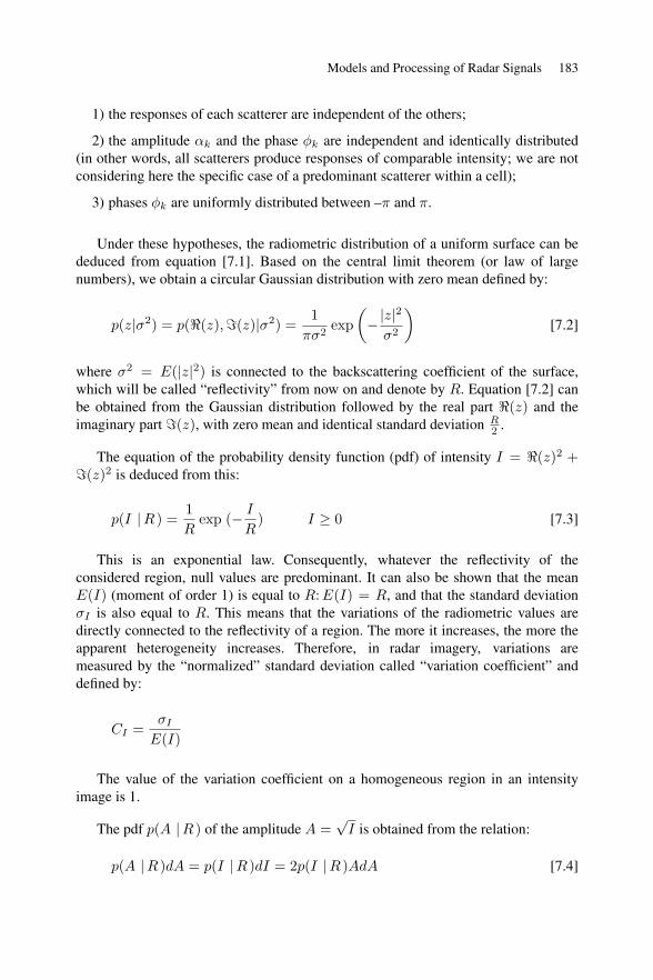
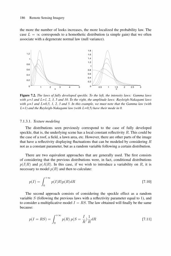
These speckle laws, both in amplitude and intensity, are illustrated in Figure 7.2,which gives the aspects for different values of the number of looks L. We see that


the more the number of looks increases, the more localized the probability law. Thecase L = ∞ corresponds to a homothetic distribution (a simple gain) that we oftenassociate with a degenerate normal law (null variance).

0

0.2

0.4

0.6

0.8

1

1.2

1 2 3 4 5u0

0.20.40.60.81

1.21.41.61.8

0.5 1 1.5 2 2.5 3u

Figure 7.2. The laws of fully developed speckle. To the left, the intensity laws: Gamma lawswith μ=1 and L=1, 2, 3, 5 and 10. To the right, the amplitude laws: Rayleigh-Nakagami lawswith μ=1 and L=0,5, 1, 2, 3 and 5. In this example, we must note that the Gamma law (withL=1) and the Rayleigh-Nakagami law (with L=0,5) have their mode in 0.

7.1.3.1. Texture modeling

The distributions seen previously correspond to the case of fully developedspeckle, that is, the underlying scene has a local constant reflectivity R. This could bethe case of a roof, a field, a lawn area, etc. However, there are other parts of the imagethat have a reflectivity displaying fluctuations that can be modeled by considering Rnot as a constant parameter, but as a random variable following a certain distribution.

There are two equivalent approaches that are generally used. The first consistsof considering that the previous distributions were, in fact, conditional distributionsp(I|R) and p(A|R). In this case, if we wish to introduce a variability on R, it isnecessary to model p(R) and then to calculate:

p(I) =+∞

0

p(I|R)p(R)dR [7.10]

The second approach consists of considering the speckle effect as a randomvariable S (following the previous laws with a reflectivity parameter equal to 1), andto consider a multiplicative model I = RS. The law obtained will finally be the samebecause:

p(I = RS) =+∞

0

p(R) p(S =I

R)1

RdR [7.11]


These reasonings are equally valid in amplitude when using the associateddistributions. For the multiplicative model, we have the following relationshipbetween the variation coefficients of the image CI , the texture of the scene CR andthe normalized speckle CS :

C2R(1 + C2

S) = C2I − C2

S [7.12]

The value of CS is 1√L

for a multi-look intensity image. We find CR = 0 (notexture) if CI = CS , and in this case intensity data have variations strictly due to thespeckle effect.

There are several hypotheses that have been studied for the R distribution:

– R = R0, area with constant reflectivity, then I follows a Gamma law withmean R0 (according to previous results); this hypothesis is well suited for physicallyhomogeneous areas.

– R follows a Gamma law, then I follows a K law; this law corresponds to aprocess of birth and death of the elementary scatterers within a resolution cell; it iswell adapted to vegetation areas;

– R follows an inverse Gamma law, then I follows a Fisher law [TIS 04]; theinterest of this distribution lies in the modeling of a wide range of textures, allowingus to model an urban environment that has strong back-scatterers as well as naturalareas.

Numerous other models have been proposed, either directly on I , or on the Rdistribution (log-normal laws, Weibull, Rice, etc.). However more complete, thedifficulty with these models comes from the increase of the number of parametersdefining the law and their estimation. A manipulation framework of thesedistributions defined in IR+, called “log-statistics”, was developed in [NIC 02]thanks to the Mellin transform, and to the Mellin convolution, which are adaptedtools for multiplicative noise (we could see, in passing, that equation [7.11] expressesa Mellin convolution). It allows us to define quantities specific to the laws on IR+:log-moments and log-cumulants, which have properties similar to the moments andtraditional cumulants of the laws defined on IR. More specifically, this frameworkallows us, through the diagram of the log-cumulants of order 2 and 3, to put the lawsin relation with one another. It also provides very advanced tools for estimating theparameters that come up in the distributions. The first parameter that must be knownis the reflectivity R of the studied area. The estimator in the sense of maximumlikelihood is given by the empirical average of intensities. As regards the number oflooks, we can either consider that it is given by the agency providing the images interms of physical parameters, or we can estimate it on the data (see the followingsection 7.1.4). In this case, the log-statistics allow us to obtain estimators with a low


variance. This is also the case for the other parameters that may intervene in thedistributions.

Another form of multi-looking is given by the multi-temporal combination of data.This leads to a very significant reduction of the speckle effect.

7.1.4. Estimating the number of looks in an image

As we have seen above, the number of looks L is the image quality parameterwhich characterizes radiometric resolution on a stationary area of the image[MAS 08]). In order to determine it, we select a homogeneous part of the image, withno apparent texture (R = Ro and CR = 0). We then have CI = CS = 1√

L, and the

calculation of the variation coefficient leads to estimating the equivalent number oflooks. In a second phase, knowing the equivalent number of looks will allow us todetermine the texture coefficient for any part of the image using equation [7.12].

In spite of a simple formulation, the number of looks is a difficult parameter toestimate. We recommend renewing the estimation for several homogeneous parts ofthe image. What is more, the slight oversampling of the image (pixel size < spatialresolution) leads to a spatial correlation between neighboring pixels, which results ina lower number of equivalent looks than expected.

Finally, we should keep in mind that the previous distributions were determinedwith the fully developed speckle hypothesis. The advent of high-resolution sensors(≤ 1m) makes it more likely to have a limited number of scatterers inside a resolutioncell (and not the “large number” required for fully developed speckle conditions). Thealternative laws mentioned previously (K laws, Weibull laws, Fisher laws, etc.) arethen more adequate to describe the statistics of the observed scene [TIS 04].

7.2. Representation of polarimetric data

Let us recall the form of the scattering matrix that was presented in Chapter 4(equation [4.53]):

¯S =Sxz Syz

Sxt Syt=

zEs10 zEs2

0

tEs10 tEs2

0

The indexes i and j of the complex coefficients Sij represent the emission mode(x or y) and the reception mode (z or t), respectively.


We have seen that, for a radar in mono-static configuration, (z = x, t = y,

ks = −kinc), we have Syx = Sxy where ¯S is the backscattering matrix. We will

adopt this configuration in the remainder of this chapter, with h instead of x (horizontaldirection), and v instead of y (vertical direction).

7.2.1. Canonical forms of the backscattering matrix

The case of a unique interaction between a wave and a dielectric or conductingsurface corresponds to single-bounce scattering (or single scattering). Concerning thepolarimetric behavior at first order, the surface can be considered as an infiniteperfectly conducting plane illuminated under normal incidence. The transmittedelectrical fields reflected from this plane undergo a phase offset of π with a totalreflection. The resulting backscattering matrix is written (with a multiplying factorincluding the phase term):

¯SSS

=1 00 1

[7.13]

For any kind of odd-bounce scattering, it is the same ¯SSS

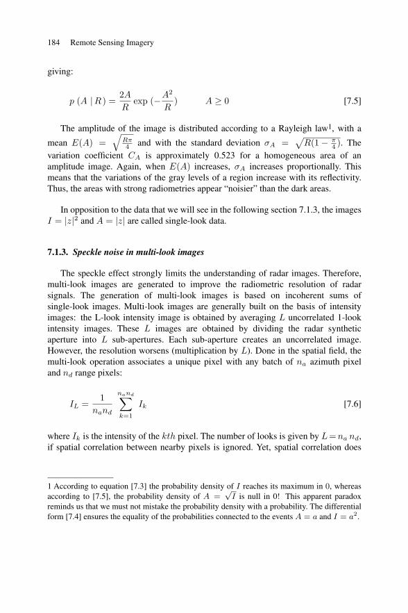
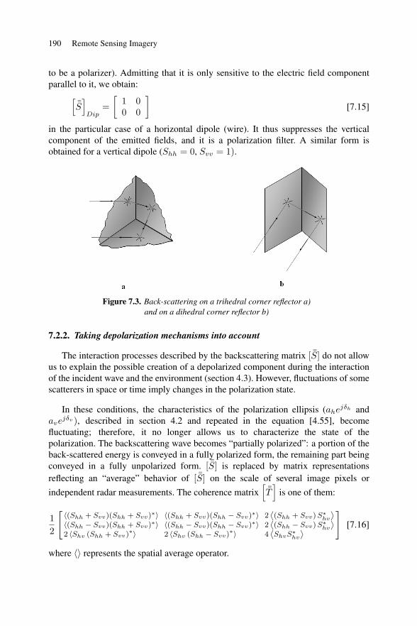
. For instance, it is thecase for third-order scattering (triple bounce) occurring on a trihedral corner reflector(Figure 7.3(a)).

The case of two successive single scattering events corresponds to double-bouncescattering or double scattering (Figure 7.3(b)). If the two surfaces are locallyorthogonal, they will create two successive specular reflections, which scatters theincident energy back to the transmitter – this is known as the dihedral ordouble-bounce effect. Double-bounce effects are extremely common in the urbanareas. The resulting backscattering matrix is written:

¯SDS

=1 00 −1

[7.14]

It is thus possible to distinguish between odd and even diffusions by usingpolarimetric measurements. Indeed, the comparison between ¯S

SDand ¯S

DRshows that Shh and Svv are in phase for odd scattering, and in phase opposition foreven scattering. Many classification algorithms are based on this property.

Diffraction effects occur on sharp edges. In this situation, the polarimetric behavioris similar to infinite straight wires or dipoles. The main feature of a dipole or wire isthat it filters out part of the transmitted polarization (to that extent, it is considered


to be a polarizer). Admitting that it is only sensitive to the electric field componentparallel to it, we obtain:

¯SDip

=1 00 0

[7.15]

in the particular case of a horizontal dipole (wire). It thus suppresses the verticalcomponent of the emitted fields, and it is a polarization filter. A similar form isobtained for a vertical dipole (Shh = 0, Svv = 1).

Figure 7.3. Back-scattering on a trihedral corner reflector a)and on a dihedral corner reflector b)

7.2.2. Taking depolarization mechanisms into account

The interaction processes described by the backscattering matrix [ ¯S] do not allowus to explain the possible creation of a depolarized component during the interactionof the incident wave and the environment (section 4.3). However, fluctuations of somescatterers in space or time imply changes in the polarization state.

In these conditions, the characteristics of the polarization ellipsis (ahejδh andave

jδv ), described in section 4.2 and repeated in the equation [4.55], becomefluctuating; therefore, it no longer allows us to characterize the state of thepolarization. The backscattering wave becomes “partially polarized”: a portion of theback-scattered energy is conveyed in a fully polarized form, the remaining part beingconveyed in a fully unpolarized form. [ ¯S] is replaced by matrix representationsreflecting an “average” behavior of [ ¯S] on the scale of several image pixels orindependent radar measurements. The coherence matrix ¯T is one of them:

1

2

(Shh + Svv)(Shh + Svv)∗ (Shh + Svv)(Shh − Svv)∗ 2 (Shh + Svv)S∗hv

(Shh − Svv)(Shh + Svv)∗ (Shh − Svv)(Shh − Svv)∗ 2 (Shh − Svv)S∗hv

2 Shv (Shh + Svv)∗ 2 Shv (Shh − Svv)

∗ 4 ShvS∗hv

[7.16]

where represents the spatial average operator.


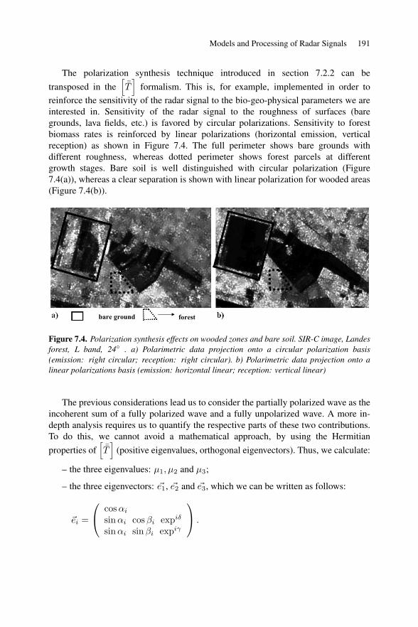
The polarization synthesis technique introduced in section 7.2.2 can betransposed in the ¯T formalism. This is, for example, implemented in order toreinforce the sensitivity of the radar signal to the bio-geo-physical parameters we areinterested in. Sensitivity of the radar signal to the roughness of surfaces (baregrounds, lava fields, etc.) is favored by circular polarizations. Sensitivity to forestbiomass rates is reinforced by linear polarizations (horizontal emission, verticalreception) as shown in Figure 7.4. The full perimeter shows bare grounds withdifferent roughness, whereas dotted perimeter shows forest parcels at differentgrowth stages. Bare soil is well distinguished with circular polarization (Figure7.4(a)), whereas a clear separation is shown with linear polarization for wooded areas(Figure 7.4(b)).

Figure 7.4. Polarization synthesis effects on wooded zones and bare soil. SIR-C image, Landesforest, L band, 24◦ . a) Polarimetric data projection onto a circular polarization basis(emission: right circular; reception: right circular). b) Polarimetric data projection onto alinear polarizations basis (emission: horizontal linear; reception: vertical linear)

The previous considerations lead us to consider the partially polarized wave as theincoherent sum of a fully polarized wave and a fully unpolarized wave. A more in-depth analysis requires us to quantify the respective parts of these two contributions.To do this, we cannot avoid a mathematical approach, by using the Hermitianproperties of ¯T (positive eigenvalues, orthogonal eigenvectors). Thus, we calculate:

– the three eigenvalues: μ1, μ2 and μ3;

– the three eigenvectors: e1, e2 and e3, which we can be written as follows:

ei =

⎛⎝ cosαi

sinαi cosβi expiδ

sinαi sinβi expiγ

⎞⎠ .


7.2.2.1. Statistics of polarimetric data

The vector S follows a zero-mean complex circular Gaussian distribution[GOO 75]:

p(S|C) =1

πd det(C)exp(−S∗tC−1S) [7.17]

where d is the dimension of S (3 or 4).

When using the empirical covariance matrix Σ locally calculated on L samples:

Σ =1

L

L

i=1

SiSt∗i

the followed distribution becomes a Wishart distribution:

p(Σ|C) =LLd|Σ|L−d exp −LTr(C−1Σ)

πd(d−1)

2 Γ(L)Γ(L− d+ 1) det(C)L

[7.18]

7.2.3. Polarimetric analysis based on the coherence matrix

7.2.3.1. Entropy

Respective weights of the polarized and unpolarized components in thebackscattered wave can be measured by the entropy H . Indeed, H locally quantifiesthe “degree of disorder” of the polarimetric response. H is equal to the logarithmicsum of the normalized eigenvalues of ¯T :

H = −3

i=1

Pi log3 (Pi) [7.19]

where Pi is given by: Pi = λ i/3

j=1

λj . H tables value between 0 and 1. The extreme

case H =0 corresponds to fully polarized backscattering mechanisms, whereas H =1corresponds to fully unpolarized backscattering mechanisms.

Another indicator is the value α, which represents quite well an average angle ofthe eigenvectors:

α =3

i=1

αiPi. [7.20]


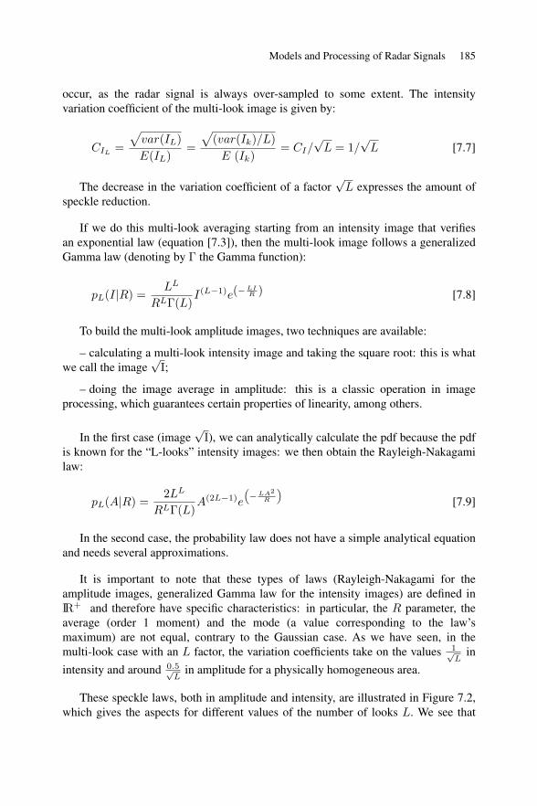
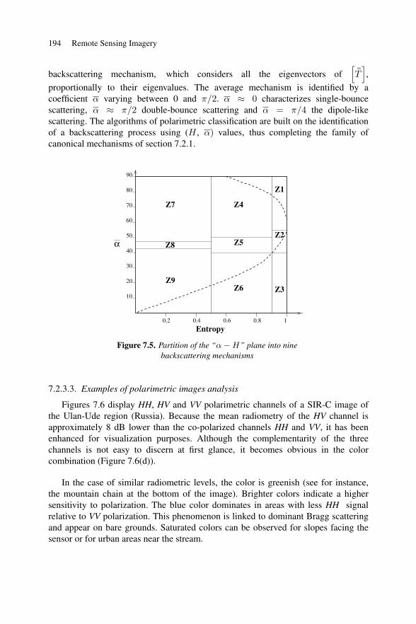
In the (H,α) diagram, we can then characterize a certain number of targets (forest,urban areas, etc.). In this diagram, the two curves give for each value of the entropythe minimal and maximal values for α (Figure 7.5).

– The low-entropy diffusion areas (H lower than 0.5) for which a singlebackscattering mechanism is predominant:

- Z9: α is lower than π4 , which corresponds to a single-bounce backscattering

mechanism (with no mechanism introducing a phase rotation of π between hh andvv). In practice, all the mechanisms described by an odd number of backscatteringsbelong to this class;

- Z7: α is higher than π4 and lower than π

2 , which corresponds to a double-bounce backscattering. In practice, all the mechanisms described by an even numberof backscatterings belong to this class;

- Z8: α is close to π4 , the proposed mechanism is a dipole backscattering.

– The middle entropy diffusion areas (H between 0.5 and 0.9):

- Z6: α is low, we have a single-bounce backscattering mechanism with effectsthat are related to the surface roughness;

- Z4: α is close to π2 , we have multiple diffusions (e.g. volume diffusion in the

forest canopy);

- Z5: α is close to π4 , which can be explained by a certain correlation between

the orientation of the scatterers.

– The high-entropy diffusion areas (H higher than 0.9):

- Z3: α is low, this area, which corresponds to α values that are higher than theupper limit, cannot be characterized by this approach;

- Z1: this area corresponds to multiple diffusions, as we may see in forestapplications;

- Z2: this area therefore corresponds to the volume diffusion by a needle-typecloud of particles (with no direction correlation). Let us note that a random noise, withno polarization effect, is represented by the values found to the farthest right of thisarea.

7.2.3.2. Dominant/average backscattering mechanism

The eigenvector associated with the largest eigenvalue of ¯T gives the dominantbackscattering mechanism. This definition does not consider if this dominantbackscattering is representative because it does not take into account the weights ofthe other contributions. [CLO 97] overcame this objection and defined the average


backscattering mechanism, which considers all the eigenvectors of ¯T ,proportionally to their eigenvalues. The average mechanism is identified by acoefficient α varying between 0 and π/2. α ≈ 0 characterizes single-bouncescattering, α ≈ π/2 double-bounce scattering and α = π/4 the dipole-likescattering. The algorithms of polarimetric classification are built on the identificationof a backscattering process using (H , α) values, thus completing the family ofcanonical mechanisms of section 7.2.1.

Z7

Z9

Z4

Z5

Z6 Z3

Z1

Z2Z8

0.2 0.4 0.80.6 1

90

80

70

60

50

40

30

20

10

α

Entropy

Figure 7.5. Partition of the “α−H” plane into ninebackscattering mechanisms

7.2.3.3. Examples of polarimetric images analysis

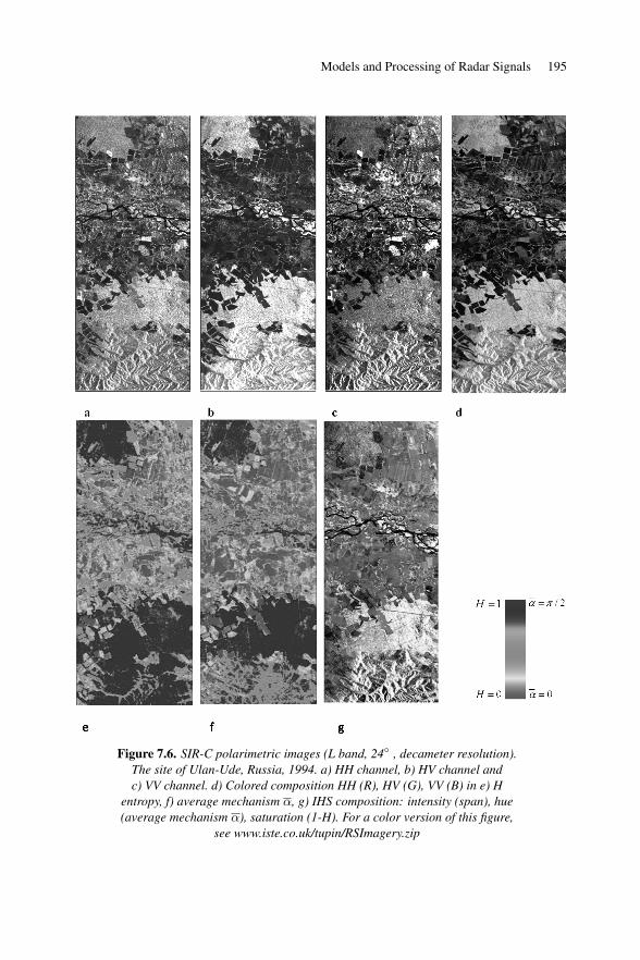
Figures 7.6 display HH, HV and VV polarimetric channels of a SIR-C image ofthe Ulan-Ude region (Russia). Because the mean radiometry of the HV channel isapproximately 8 dB lower than the co-polarized channels HH and VV, it has beenenhanced for visualization purposes. Although the complementarity of the threechannels is not easy to discern at first glance, it becomes obvious in the colorcombination (Figure 7.6(d)).

In the case of similar radiometric levels, the color is greenish (see for instance,the mountain chain at the bottom of the image). Brighter colors indicate a highersensitivity to polarization. The blue color dominates in areas with less HH signalrelative to VV polarization. This phenomenon is linked to dominant Bragg scatteringand appear on bare grounds. Saturated colors can be observed for slopes facing thesensor or for urban areas near the stream.


Figure 7.6. SIR-C polarimetric images (L band, 24◦ , decameter resolution).The site of Ulan-Ude, Russia, 1994. a) HH channel, b) HV channel andc) VV channel. d) Colored composition HH (R), HV (G), VV (B) in e) H

entropy, f) average mechanism α, g) IHS composition: intensity (span), hue(average mechanism α), saturation (1-H). For a color version of this figure,

see www.iste.co.uk/tupin/RSImagery.zip


Entropy estimated on a 7 × 7 pixel analysis window is displayed in Figure 7.6(e)for the SIR-C image. Almost fully unpolarized waves present high entropy (e.g. themountain in the lower part of the image). These high entropy values generally reflectdominant volume scattering. The high values of the HV signal confirm this hypothesis.In addition, the received signal is practically insensitive to transmission and receptionpolarizations because the HH, VV and HV radiometric values are evenly distributed(Figure 7.6(d)). Similar results can be observed at the C band, although entropy is onaverage slightly higher than at the L band, making the C band polarimetric analysismore difficult.

The coefficient α of the SIR-C image (Figure 7.6(f)) is strongly correlated toentropy. When the back-scattered signal is highly polarized, the three polarizationchannels are significantly complementary, and it induces low entropy. The concernedareas correspond principally to surfaces producing a simple dominant diffusion,associated with a low α value.

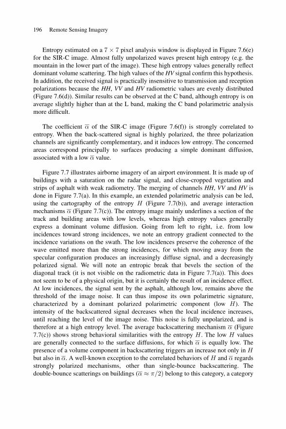
Figure 7.7 illustrates airborne imagery of an airport environment. It is made up ofbuildings with a saturation on the radar signal, and close-cropped vegetation andstrips of asphalt with weak radiometry. The merging of channels HH, VV and HV isdone in Figure 7.7(a). In this example, an extended polarimetric analysis can be led,using the cartography of the entropy H (Figure 7.7(b)), and average interactionmechanisms α (Figure 7.7(c)). The entropy image mainly underlines a section of thetrack and building areas with low levels, whereas high entropy values generallyexpress a dominant volume diffusion. Going from left to right, i.e. from lowincidences toward strong incidences, we note an entropy gradient connected to theincidence variations on the swath. The low incidences preserve the coherence of thewave emitted more than the strong incidences, for which moving away from thespecular configuration produces an increasingly diffuse signal, and a decreasinglypolarized signal. We will note an entropic break that bevels the section of thediagonal track (it is not visible on the radiometric data in Figure 7.7(a)). This doesnot seem to be of a physical origin, but it is certainly the result of an incidence effect.At low incidences, the signal sent by the asphalt, although low, remains above thethreshold of the image noise. It can thus impose its own polarimetric signature,characterized by a dominant polarized polarimetric component (low H). Theintensity of the backscattered signal decreases when the local incidence increases,until reaching the level of the image noise. This noise is fully unpolarized, and istherefore at a high entropy level. The average backscattering mechanism α (Figure7.7(c)) shows strong behavioral similarities with the entropy H . The low H valuesare generally connected to the surface diffusions, for which α is equally low. Thepresence of a volume component in backscattering triggers an increase not only in Hbut also in α. A well-known exception to the correlated behaviors of H and α regardsstrongly polarized mechanisms, other than single-bounce backscattering. Thedouble-bounce scatterings on buildings (α ≈ π/2) belong to this category, a category


that is however too rare statistically to shake off the impression of similarity betweenH and α observed in numerous images.

Figure 7.7. ONERA/RAMSES L band image, 5-m resolution, acquired over anairport area. a) Colored composition HH (R), HV (G), VV (B). b) H entropy,

c) average mechanism. d) IHS composition intensity (span), hue (averagemechanism α), saturation (1-H). For a color version of this figure, see

www.iste.co.uk/tupin/RSImagery.zip

7.2.4. Synoptic representation of polarimetric information

Due to the vectorial dimension of polarimetric channels with more than threedimensions, it is impossible to display a complete representation for it. In case ofhigh entropy, the phase information is useless, and there is no need to have acomplete representation of the information. In [IMB 99], an adaptive visualizationsystem inspired from interferometry is proposed, based on a decomposition intointensity-hue-saturation (IHS)2. This system automatically reduces the representationof the polarimetric information to its radiometric part whenever the signal is stronglyunpolarized.

2 The intensity associated with every pixel of the image is related to its radiometric content(that is, its “black&white” component), the saturation refers to its coloring level and the hueto the actual color itself. The IHS representation is another way of presenting the tri-chromaticdecomposition red-green-blue of a color image.


– The intensity channel carries a layer of radiometric information, for example thespan image, the incoherent sum of radiometries:

SPAN = |HH|2 + |V V |2 + 2 |HV |2

It thus provides a gray-level background image.

– The saturation channel is controlled by the local polarization state, revealed bythe H entropy (section 7.2.3.1) or the polarization degree P (section 4.1.3.3). A highentropy leads to a low saturation (and vice versa), that is to an image that is locally ingray-levels, with an exclusively radiometric content. The law connecting the saturationis usually linear (S = 1−H), although more subtle relations can be involved.

– Finally, because the decreasing entropy colors the image gradually, the Huechannel will associate with each pixel a color related to the local polarimetric behavior(e.g. via the coefficient α), but only when this is meaningful.

Based on such a representation, the discrimination between polarized andunpolarized areas is easier. In the SIR-C image (Figure 7.6(g)), within theunpolarized maelstrom at the bottom of the image, only the mountain crests retainsome wave coherence. On the contrary, the central part of the image presents mostlypolarized surface scattering. In the airborne case (Figure 7.7(d)), the IHSrepresentation emphasizes the incidence effect on the polarization of backscatteredwaves. The bluish points correspond to both low entropy values, and high α values,meaning polarized double-bounce backscattering created by built-up areas.

7.3. InSAR interferometry and differential interferometry (D-InSAR)

The geometric aspects of interferometry and D-InSAR will be detailed in Chapters8 and 9.

Radar interferometry (InSAR) is based on geometric information hidden in thephase of a pixel, accessible with SLC Single Look Complex data. Phase informationcan be divided into two parts. The first part is linked to the electromagnetic propertiesof the target and is called the intrinsic phase, whereas the second part is linked to thedistance between the sensor and the target.

With single-phase information, it is generally not possible to separate these twopieces of information and retrieve the measurement. However, when twomeasurements of the same pixel φ1 and φ2 are available, it is possible by subtractionto recover the geometric information.

If φ2 is acquired with exactly the same position of the sensor, we will of coursehave φ2 − φ1 = 0, unless the point observed has slightly moved while remaining in


the same radar bin. Generally, the second acquisition is done with a slightly differentincidence angle, allowing us to recover not only the potential motion information, butalso the topography in the phase difference. Interferometry exploits this property tobuild digital terrain models (DTM). D-InSAR is concerned with ground movements,by combining two acquisitions with an existing DTM, or by exploiting a set ofacquisitions (at least three).

In this section, we will admit that the phase difference contains height ormovement information, and we will be interested in the distributions followed by thisphase.

7.3.1. Statistics of interferometric data

Interferometry is the measurement of two complex data z1 and z2, which can beput into a complex vector Z , analogously to what was done in the previous sectionwith the four polarimetric components (equation [7.17]). We may again consider thezero mean circular Gaussian model, and the distribution of Z is written:

pz (Z|Cz) =1

π2 det (Cz)exp −Zt∗ C−1

z Z [7.21]

Cz is the covariance matrix of Z, also called the coherence matrix. It is written:

Cz =|z1|2 z1z

∗2

z∗1z2 |z2|2 [7.22]

ρ12, the complex correlation coefficient (or degree of coherence) is written:

ρ12 =z1z

∗2

|z1|2 |z2|2= D ejβ

D is simply the coherence, and β the actual offset between the components of Z.Defining the reflectivities R1 = |z1|2 and R2 = |z2|2 , Cz can then be written:

Cz =R1

√R1 R2 D ejβ√

R1 R2 D e−jβ R2.

For D = 1, C−1z is written:

C−1z =

1

R1R2 (1−D2)

R2 −√R1 R2 D ejβ

−√R1 R2 D e−jβ R1

.


For two complex values z1 and z2, equation [7.21] is given by:

p(z1, z2 |R1, R2, D, β) = 1π2R1R2(1−D2)

exp − 11−D2

z1z∗1

R1+

z2z∗2

R2− D(z1z∗

2ejβ + z∗

1z2e−jβ)√

R1R2.

[7.23]

If, instead of considering z1 and z2 values, we consider the joint distribution of Σz

elements, the empirical co-variance matrix:

Σz = Z Zt∗ =I1 I12e

jϕ

I12e−jϕ I2

.

We can then express the joint distribution of the elements of Σz depending on thereflectivities R1 and R2, and of the complex coherence Dejβ as:

p(I1, I2, I12, ϕ|R1, R2, D, β) = 1π2R1R2(1−D2)

exp − 11−D2

I1R1

+ I2R2

− 2DI12 cos(ϕ−β)√R1R2

.[7.24]

We can deduce from this equation the distributions of the anti-diagonal term of theempirical covariance matrix I12e

jϕ, called complex interferogram (Figure 7.8).

In practice, rather than calculating z1z∗2 = I12e

jϕ, a spatial averaging on Lsamples is computed (sometimes called somewhat improperly complex multilooking,L being the “number of looks”) in order to obtain an empirical spatial coherence,denoted by d:

dejϕ =

Lk=1 z1,kz

∗2,k

Lk=1 z1,kz

∗1,k

Lk=1 z2,kz

∗2,k

=I12√I1 I2

ejϕ L ≥ 2. [7.25]

This coherence measures the correlation between the complex data used tocalculate the interferometric phase. It comprises in [0, 1], the higher values ensuring agood quality of the measured interferometric phase, whereas the lower valuesindicate the decorrelation between the two images z1 and z2. Several factors cancause this decorrelation: the absence of the measured signal (shadow area), thevariations of the acquisition geometry, the temporal variations of the ground(vegetation areas, human modifications, etc.), the variation of the atmosphericconditions between the two acquisitions and so on. We will return to these in a futurechapter.


Starting from equation [7.24], the law verified by the empirical coherence obtainedby the space averaging on L samples is deduced:

p(d|D,L) = 2(L− 1)(1−D2)Ld(1− d2)L−22F1(L,L; 1; d

2D2)

as well as the pdf of the phase ϕ:

p(ϕ|D, β, L) =(1−D2)L

2π

1

2L+ 12F1 2, 2L;L+

3

2;1 +D cos(ϕ− β)

2[7.26]

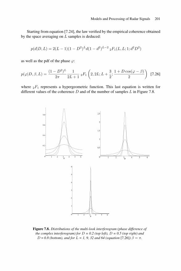
where 2F1 represents a hypergeometric function. This last equation is written fordifferent values of the coherence D and of the number of samples L in Figure 7.8.

0

0.2

0.4

0.6

0.8

1 2 3 4 5 6ϕ 0

0.5

1

1.5

2

2.5

1 2 3 4 5 6ϕ

0

1

2

3

4

5

6

1 2 3 4 5 6ϕ

Figure 7.8. Distributions of the multi-look interferogram (phase difference ofthe complex interferogram) for D = 0.2 (top left), D = 0.5 (top right) andD = 0.8 (bottom), and for L = 1, 9, 32 and 64 (equation [7.26]) β = π.


The spatial averaging (called complex multi-looking) is usually applied to computethe interferogram because of the phase noise (see Figure 7.8). However, this averagingis done at the cost of the spatial resolution of the interferogram. There are severalsolutions that have been explored for selecting the best samples to be averaged andthus reduce the phase noise without damaging the resolution.

7.4. Processing of SAR data

This chapter aimed to present distributions followed by different radar data. Thesemodels are crucially important, as they will be the basis of the processing methods.

As regards phase de-noising, or more precisely, the estimation of relevantparameters (reflectivity, interferometric phase, coherence, etc.), methods will takeinto account these distributions in order to select the similar samples and combinethem. For example, in [DEL 11a] an adaptation of the non-local means is proposed toimprove the complex multi-looking.

Classification approaches are generally expressed in a Bayesian framework andrely on the distributions we have studied previously. Criteria such as maximumlikelihood or a posteriori maximum are used (section 5.6.1). Similarly, detectingrelevant objects such as targets will rely on hypotheses tests, defined to use theefficiency of these statistic models (section 5.5.1).

7.5. Conclusion

Radar image processing techniques rely very heavily on the statistics presented inthis chapter. Among open issues, it is worth noting that the distributions will neverbecome Gaussian whatever the number of looks. This means that processingapproaches relying on additional white Gaussian noise assumptions will never beperfectly adapted to radar imagery, whatever may be the noise reduction techniqueused.

Another important issue is currently unsolved: geometric aspects are usually nottaken into account because they require a DTM or a digital elevation model (DEM).In particular, not taking into account the local slope of the ground or of the imagedobjects makes processing less effective. Iterative approaches are necessary tointroduce height information. When a DTM or a DEM are available, more and moreprocessing techniques introduce a correction depending on the local slope (e.g. inpolarimetry where this correction is essential).

Documents

Remote Sensing Imagery (Tupin/Remote Sensing Imagery) || Models and Processing of Radar Signals