Embed Size (px)
Citation preview
REMOTE SENSING AND MODELING OF SNOW PROCESSES
Muhammad Jahanzeb Malik
Examining committee: Prof.dr.ing. W. Verhoef University of Twente Prof.dr. A.K. Skidmore University of Twente Dr. M. Ek NCEP/NOAA Prof. J. Wen Chinese Academy of Sciences Dr. C. Notarnicola Institute for Applied Remote Sensing, Italy Prof. M.J. Polo Universidad de Córdoba ITC dissertation number 254 ITC, P.O. Box 6, 7500 AA Enschede, The Netherlands ISBN 978-90-365-3751-3 DOI: 10.3990/1.9789036537513 Cover designed by Benno Masselink Photos on cover page are from the 2002-2003 NASA Cold Land Processes Experiment (CLPX) Printed by ITC Printing Department Copyright © 2014 by M.J. Malik
REMOTE SENSING AND MODELING OF SNOW PROCESSES
DISSERTATION
to obtain the degree of doctor at the University of Twente,
on the authority of the rector magnificus, prof.dr. H. Brinksma,
on account of the decision of the graduation committee, to be publicly defended
on Friday 3 October 2014 at 16.45 hrs
by
Muhammad Jahanzeb Malik
born on 15th December, 1980
in Karachi, Pakistan

This thesis is approved by Prof. dr. Bob Su, promoter Dr. ir. Rogier van der Velde, co-promoter Dr. Zoltan Vekerdy, co-promoter

Preface After completing my bachelors in Civil Engineering (2002), I dreamt to get higher education either from Europe or U.S. The dream realized in 2007 when Higher Education Commission Pakistan (HEC) awarded me a “Maters leading to PhD” scholarship (17 February, 2007) and ITC enrolled me as a Masters student in September, 2007.
The discussions with Mr. Abdul Nasir (late; one of my bosses) before coming to ITC defined a broad objective for my research: to use remote sensing for water resources management. Pakistan is a country that depends on snow/ice melt for fresh water supply. This fact narrowed down the objective to “remote sensing of snow” and set two thesis’ keywords: Remote sensing and Snow.
During Masters, my interest in microwave took me to Dr. ir. Rogier van der Velde; I did my MSc thesis with him together with Prof. Bob Su and Dr. Zoltan Vekerdy. During different meetings and occasions, I heard from Bob and Rogier about land surface modeling and data assimilation. These discussions developed my interest in land surface modeling and set the third and last keyword of the thesis: “modeling”. Therefore, the thesis – in your hands now – is titled as “Remote sensing and Modeling of Snow Processes”.
The thesis’ contents were kept changing throughout the research, as I was working on many different ideas including to use active microwave remote sensing for snow water equivalent retrieval, to simulate snow cover dynamics over the Tibet and Himalayas. Especially, in the last stages of my PhD, I met with Dr. Tim Hoar in the CAHMDA workshop (8-13 Jul, 2012 at ITC) and tried to study snow cover dynamic and its impact on the sub-continent. But, the constraints (availability of model source codes, data sets, time) restrict this thesis to limited electromagnetic spectrum (optical remote sensing), spatial extents, and snow variables (snow albedo and snow coverage). Despite these constraints, the thesis results in interesting but improved approaches for retrieval, simulation, and assimilation of snow properties. Let’s have a look how all these work together in this thesis.

ii
Acknowledgements This research was supported financially by the Higher Education Commission (HEC), Pakistan and administratively by the NUFFIC, The Netherlands and Pakistan Space and Upper Atmosphere Research Commission (SUPARCO). I am extremely grateful for the support of these institutions throughout the research period.
I would never be able to complete this thesis without the invaluable contributions of many individuals to whom I have the pleasure of expressing my gratitude:
Foremost, my deepest gratefulness is due to my promoter Prof. dr. Bob Su and my supervisors Dr. Zoltan Vekerdy and Dr. ir. Rogier van der Velde. Their thought-provoking scientific suggestions, accurate guidance, and huge encouragements throughout the study have been invaluable to me. I am extremely grateful of Rogier for invaluable and intensive working with me on improving the manuscripts’ quality and answering reviewers’ comments, which helped me a lot to improve my writing and presentation skills and thus to get good quality publications and this thesis also.
My heartiest and sincere gratitude are paid to Mr. Ahmed Bilal (Chairman), Mr. Raza Hussain (Former Chairman), Mr. Imran Iqbal (Member SAR), Mr. Shafiq Ahmed (DG), Mr. Jawed Ali Qurashi, Mr. Arshad H Siraj, Mr. Abdul Nasir (late), Mr. Ashar H. Lodi, and all other office colleagues for motivating and encouraging me throughout the studies.
Cordial thanks to Amjad Ali, Haris A. Bhatti, M. Imran, M. Yaseen, M. Shafique, Mobushir R. Khan, Rehmat Ullah, Saleem Ullah, Salma Anwar, Sumbal Bahar Saba, and Zahir Ali for their invaluable, unforgettable, and strong social support and company. I also pay high regards to all other Pakistani students met in ITC during the research period.
I also wish my deepest appreciations to all my PhD fellow students for their friendly attitude during various visits, workshops, and extra curriculum activities. Sincere acknowledgements are made to all members of WRS – especially to Ms. Anke de Koning and Ms. Tina Butt-Castro; ITC’s research coordination (that includes Library also) and student affairs for their continuous support.
Finally, I would like to give special and heartiest thanks to my loving parents, wife, brothers and sisters, and other family members for their full support, prayers, and good wishes that made me able to complete this research. To my little daughter Sarah, born when I was working on my third and last
iii

publication, I would like to express my love and thanks for always cheering me up.
iv

Table of Contents Preface ................................................................................................. i Acknowledgements ............................................................................... iii List of figures ...................................................................................... vii List of tables........................................................................................ xi 1 Introduction ................................................................................... 1
1.1 Background ............................................................................ 1 1.2 Satellite-based Remote Sensing ................................................ 3 1.3 Land Surface Models ................................................................ 4 1.4 Research objective .................................................................. 6 1.5 Research questions .................................................................. 6 1.6 Thesis structure ...................................................................... 7
2 Semi-empirical approach for estimating broadband albedo of snow ....... 9 2.1 Introduction .......................................................................... 10 2.2 Model description .................................................................. 11
2.2.1 Reflectance pattern analysis ................................................ 12 2.2.2 Geometric specifications of the triangular pattern ................... 17 2.2.3 Physical and mathematical description of the triangular pattern 18
2.3 Results and discussion ........................................................... 22 2.3.1 Theoretical assessment ....................................................... 23 2.3.2 Practical assessment .......................................................... 28
2.4 Conclusion ............................................................................ 34 3 Prospects of dual view remote sensing for fractional snow cover mapping ...................................................................................... 35
3.1 Introduction .......................................................................... 36 3.2 Fractional Snow cover mapping with existing algorithm .............. 37
3.2.1 Study areas ....................................................................... 37 3.2.2 Datasets ........................................................................... 38 3.2.3 Accuracy assessment .......................................................... 39
3.3 Fractional Snow cover mapping at pixel scale using the Sentinel-3, SLSTR- dual view approach ............................................................... 45
3.3.1 Set-up for TOA reflectance simulation ................................... 47 3.3.2 Relation between 𝐟𝒔𝒏 ∗ and 𝒇𝒔𝒏𝒔𝒖𝒓𝒇𝒂𝒄𝒆 ................................. 49
3.4 Discussion and conclusions ..................................................... 55 4 Improving modeled snow albedo estimates during the spring melt season ........................................................................................ 57
4.1 Introduction .......................................................................... 58 4.2 Study sites ........................................................................... 60 4.3 Data sets .............................................................................. 62 4.4 Measured snow albedo decay during melting period ................... 64 4.5 The Noah LSM ....................................................................... 66
4.5.1 Snowpack physics .............................................................. 66 4.5.2 Snow albedo parameterizations ........................................... 68
v

4.5.3 Calibration of snow albedo parameterizations ........................ 70 4.6 Noah simulations ................................................................... 73
4.6.1 Snow albedo ...................................................................... 73 4.6.2 Snow depth ....................................................................... 77 4.6.3 Upward shortwave radiation ................................................ 79 4.6.4 Snowmelt .......................................................................... 81
4.7 Implications at large scale ...................................................... 82 4.8 Conclusion ............................................................................ 87
5 Assimilation of satellite-observed snow albedo in a land surface model 89 5.1 Introduction .......................................................................... 90 5.2 CLPX .................................................................................... 91
5.2.1 Study area ........................................................................ 91 5.2.2 Ground measurements ....................................................... 92
5.3 Satellite-observed snow albedo products .................................. 93 5.4 Noah snow process simulations ............................................... 94
5.4.1 Model physics .................................................................... 94 5.4.2 Open-loop simulation.......................................................... 95
5.5 Snow albedo assimilation ....................................................... 98 5.5.1 Assimilation approach ......................................................... 98 5.5.2 Updated simulations .......................................................... 100 5.5.3 Simulations for NM and NP sites .......................................... 104
5.6 Conclusions and discussion .................................................... 106 6 Thesis’ conclusions ....................................................................... 109
6.1 Satellite observation of snow properties .................................. 109 6.2 Land surface modeling .......................................................... 111 6.3 Use of observations for modeling ............................................ 112 6.4 Limitations and recommendations .......................................... 114 6.5 Final remarks ....................................................................... 115
Bibliography ...................................................................................... 117 Summary .......................................................................................... 129 Samenvatting .................................................................................... 131 ITC Dissertation List ........................................................................... 133
vi

List of figures
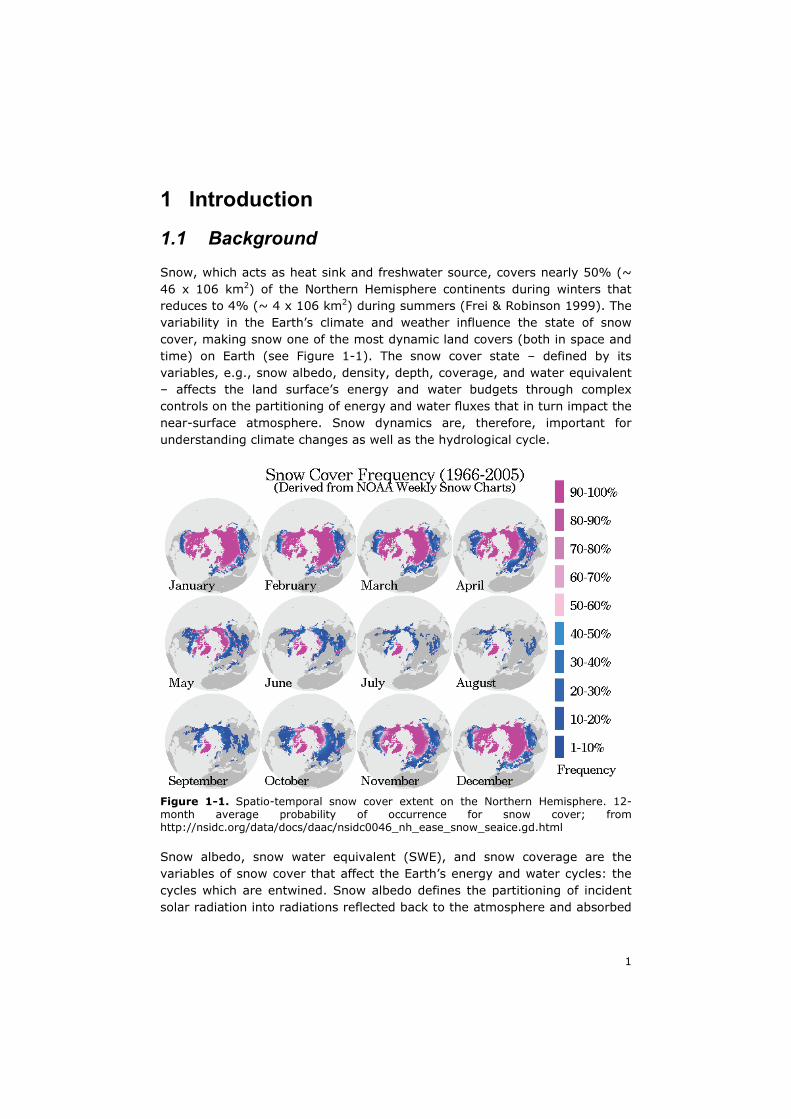
Figure 1-1. Spatio-temporal snow cover extent on the Northern Hemisphere. 12-month average probability of occurrence for snow cover; from http://nsidc.org/data/docs/daac/nsidc0046_nh_ease_snow_seaice.gd.html . 1
Figure 1-2. Flowchart of research and thesis structure ............................... 7
Figure 2-1. Scatter plot of simulated directional reflectance (Rλ) and spectral albedo (as, λ) ....................................................................................... 13
Figure 2-2. Strength of the relation between near infrared albedo and spectral albedo at various wavelengths .................................................. 14
Figure 2-3. Scatter plot showing directional reflectance patterns as a function of snow grain radii and spectral albedo (as, λ) .......................................... 15
Figure 2-4. RS imaging geometry in the principal plane (in the figure φrel= 0°) .................................................................................................... 16
Figure 2-5. Plot showing the relationship between reflectance (Rλ) and spectral albedo (as, λ) at centroids ......................................................... 16
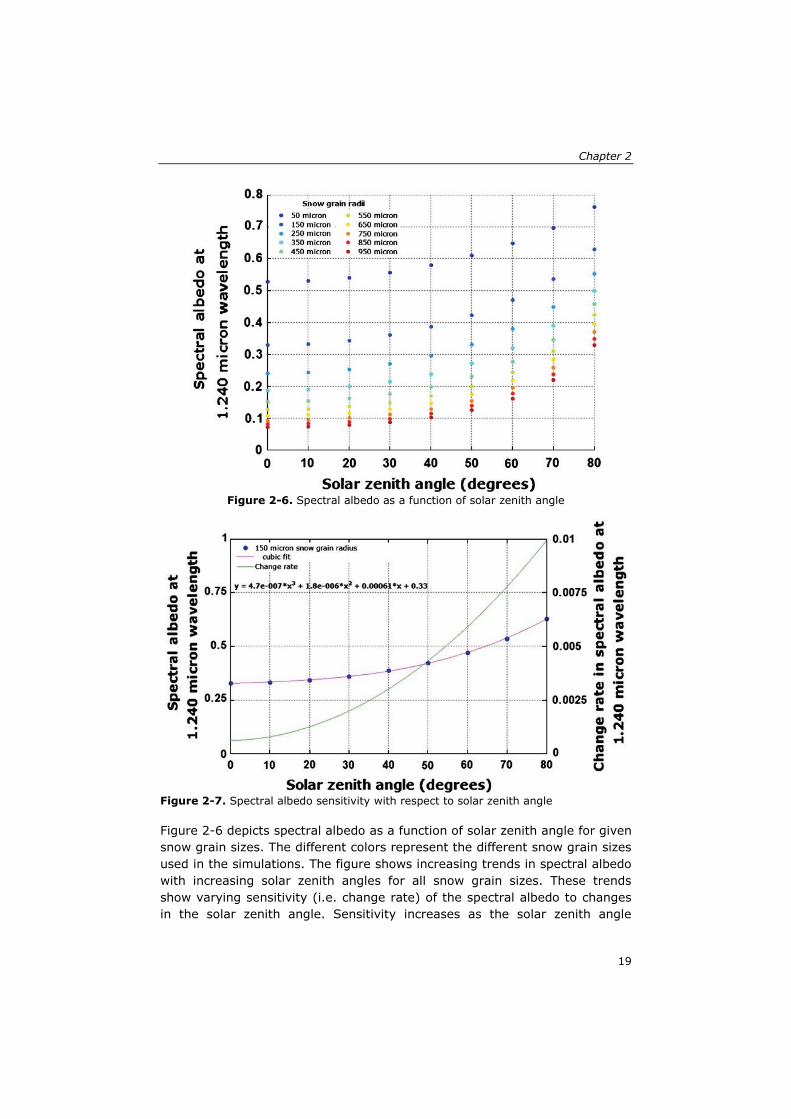
Figure 2-6. Spectral albedo as a function of solar zenith angle .................. 19
Figure 2-7. Spectral albedo sensitivity with respect to solar zenith angle .... 19
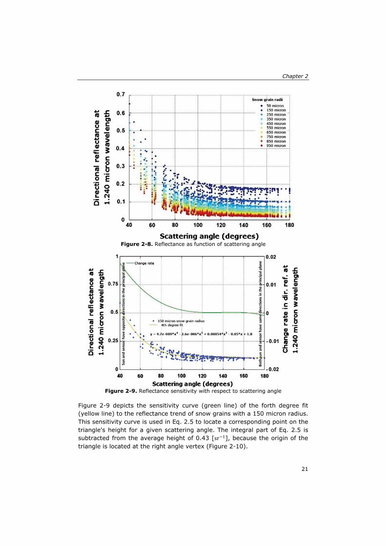
Figure 2-8. Reflectance as function of scattering angle............................. 21
Figure 2-9. Reflectance sensitivity with respect to scattering angle ............ 21
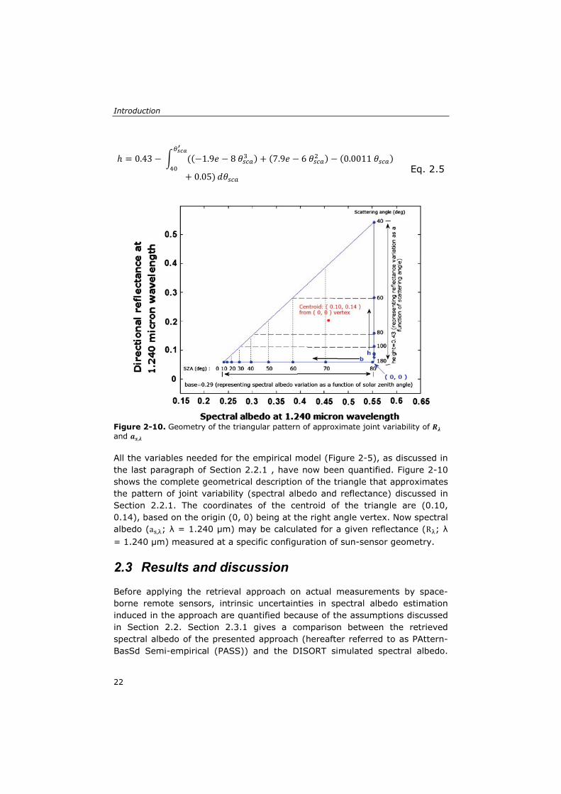
Figure 2-10. Geometry of the triangular pattern of approximate joint variability of Rλ and as, λ ....................................................................... 22
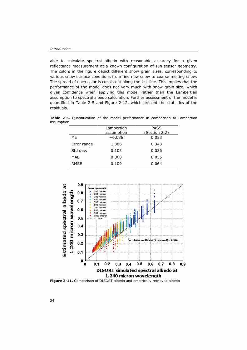
Figure 2-11. Comparison of DISORT albedo and empirically retrieved albedo ........................................................................................................ 24
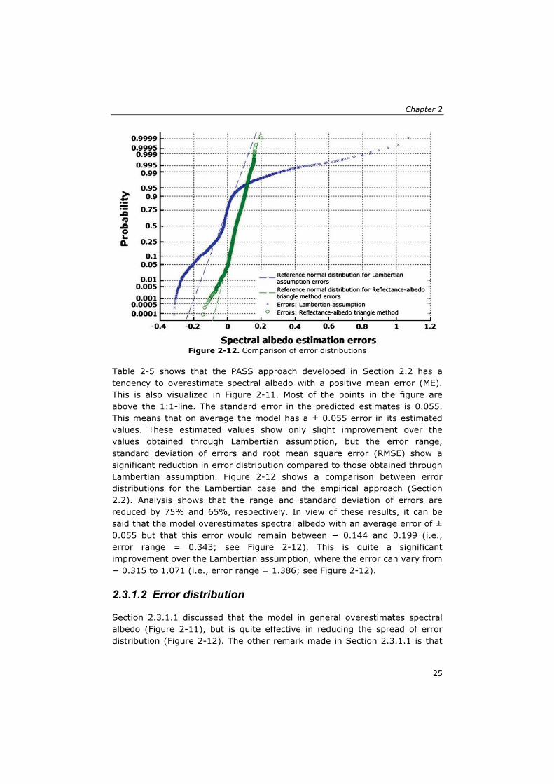
Figure 2-12. Comparison of error distributions ........................................ 25
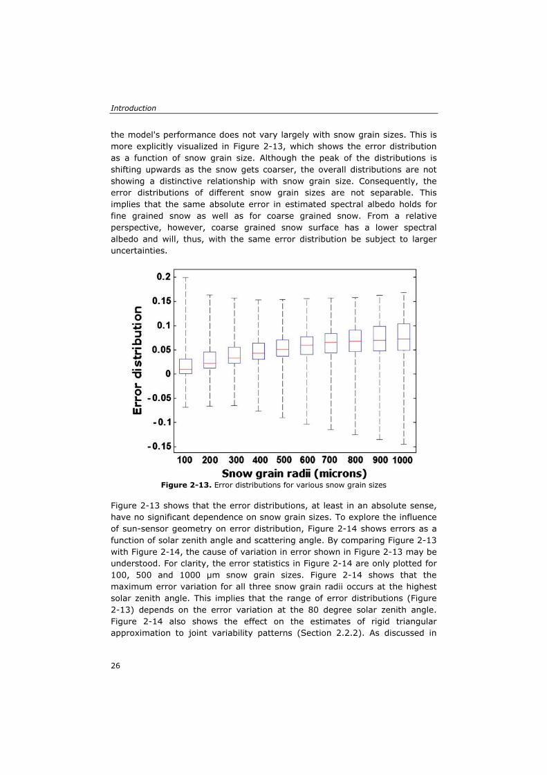
Figure 2-13. Error distributions for various snow grain sizes ..................... 26
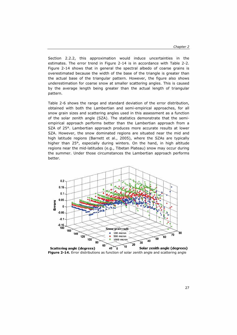
Figure 2-14. Error distributions as function of solar zenith angle and scattering angle .................................................................................. 27
Figure 2-15. Relationship between spectral albedo and spectrally integrated infrared albedo ................................................................................... 31
Figure 2-16. Comparison of RS retrieved broadband albedo with the measured albedo. Plot (a) shows result of the developed semi-empirical model and (b) is the comparison of MOD10 daily snow product for the test sites .................................................................................................. 32
Figure 3-1. Atmospheric visibility conditions during days of Landsat acquisitions ........................................................................................ 39
Figure 3-2. Snow covered and snow-free land surface spectra .................. 40
Figure 3-3. Fractional snow estimation accuracy of NDSI based linear empirical relation ................................................................................ 41
vii
Figure 3-4. Comparison of FSC estimates from MOD10A1 with the FSC estimates retrieved from Landsat .......................................................... 42
Figure 3-5. Uncertainty of MOD10A1 algorithm ....................................... 43
Figure 3-6. Surface spectra (MOD09GA) when MOD10A1-FSC-SDS overestimates snow fraction up to 35% ................................................. 44
Figure 3-7. Surface spectra (MOD09GA) when MOD10A1-FSC-SDS underestimates snow fraction up to 25% ............................................... 45
Figure 3-8. Spectral signatures for snow and background land surface....... 48
Figure 3-9. Composite surface reflectance from varying FSC at pixel scale . 48
Figure 3-10. Relationship between TOA retrieved FSC from nadir view and on land surface FSC ................................................................................. 50
Figure 3-11. Slope (i.e., between TOA retrieved FSC nadir view and on surface FSC; Figure 3-10) variation for varying visibility and solar zenith angle ................................................................................................. 51
Figure 3-12. Dependence of slope on solar zenith angle ........................... 52
Figure 3-13. Slope dependence on atmospheric visibility for different solar zenith angles ...................................................................................... 53
Figure 3-14. Comparison of retrieved pattern with the MODTRAN pattern .. 54
Figure 4-1. In situ snow albedo and depth measurements for the alpine snow sites. a), b), c), and d) show the measurements at RB, RS, RW, and CDP sites, respectively. Measurements for the FA site reveal similar patterns and are not shown for brevity. The left-hand and right-hand vertical lines highlight the instants when the albedo reaches the minimum value of optically thick snowpack and when the snowpack becomes optically thin, respectively. The top horizontal line indicates the minimum albedo value of optically thick snowpacks, and the bottom horizontal line is the depth up to the melting snowpack remains optically thick. ........................................ 65
Figure 4-2. In situ measurements of snow albedo and snow depth for the prairie (NI and Namco) and tundra (Ivo) sites. a), b), and c) show the measurements for the NI, Ivo, and Namco sites, respectively. .................. 66
Figure 4-3. Behavior of snow albedo parameterizations as a function of time since the onset of snowmelt. a) shows the parameterizations with default and calibrated parameter sets. b) illustrates the interpretation of parameters of the VAS parameterization using the measurements of the RB site as an example............................................................................................. 72
Figure 4-4. Root Mean Squared Error computed between measurements collected at the RB site and calculation with the VAS parameterization with a values ranging from 20-30 days and c (minimum snow albedo) values from 0.4 to 0.5 as indication for parameterization´s sensitivity. ....................... 72
Figure 4-5. Evolution of observed and simulated snow albedo for the alpine sites. a), b), c) and d) are for RB, RS, RW, and CDP sites, respectively. ..... 74
viii
Figure 4-6. Scatter plots of snow albedo simulations versus in situ measurements for alpine snow conditions: a) BATS, b) CLASS, c) Noah’s default parameterization, and d) VAS parameterization. .......................... 75
Figure 4-7. Evolution of observed and simulated snow albedo for the tundra (a, Ivo site) and prairie (b, NI site) snow conditions. ............................... 77
Figure 4-8. Time series of simulated and measured snow depths for alpine snow conditions: a) RB site , b) RS site, c) RW site, and d) CDP site. ......... 78
Figure 4-9. Time series of simulated and measured snow depths for tundra (Ivo) and prairie (NI) snow conditions: a) Ivo site and b) NI site. ............. 79
Figure 4-10. Measured and simulated upward shortwave radiative flux for the RB site. a) shows the period near the start of snow melting, and b) shows the period at the end of snow melting. ........................................................ 80
Figure 4-11. Snowmelt at CDP site: measured and simulated. a) is the time series of the 1999 springtime. b) and c) show scatter plots of simulations versus measurements of the 1999 and 2009 springtimes, respectively. ..... 82
Figure 4-12. Map showing the upper and lower Colorado River basins outlined in solid black and gray lines, respectively. 1) the black-line is the Colorado River, 2) is the Green River, and 3) is the San Juan river. ........................ 83
Figure 4-13. Noah simulated SCF and SCD from 1-Oct 2009 to 30 Sept 2010 for the UCRB. a) shows time series of SCF simulated by Noah with the default and VAS parameterizations for snow albedo, SCF difference yielded with the two parameterizations, and SCF derived from 8-day MODIS snow cover product (MOD10A2). b) and c) show the SCD simulated with the Noah’s default and VAS parameterizations, respectively, and d) shows the difference [i.e., b) minus c)] between the SCD simulated by Noah with the two parameterizations. .............................................................................. 85
Figure 4-14. Noah simulated ET for the UCRB. a) and b) show accumulated ET produced respectively with the noah’s default and VAS parameterizations from 1-Feb to 30-Jun, 2010; c) shows difference [i.e., b) minus a)] in the accumulated ET produced by Noah with the two parameterizations. .......... 86
Figure 4-15. The Noah LSM simulated runoff (surface runoff + drainage) production with the VAS and default snow albedo parameterizations, and their difference. Values are averages across all basin grid cells (not routed flows). ............................................................................................... 86
Figure 5-1. In situ measured and Noah simulated for (a) snow depth and (b) snow albedo plotted over time along the with the NLDAS-2 precipitation. DOWY starts 1 Oct and ends 30 Sep. ..................................................... 97
Figure 5-2. Noah-simulated snow albedo plotted against in situ measurements. The points show average values of ±2 h at 1900 UTC of each day. .................................................................................................. 98
Figure 5-3. Illustration of DI scheme for snow albedo assimilation. The black solid line shows the open-loop Noah simulation. The gray dashed and gray dashed–dotted lines are for the updated surface albedo simulations. Gray dashed line receives updates from the PASS approach (+ symbol), and gray
ix
dashed–dotted line obtains updates from MOD10A1 (x symbol). Gray dotted line represents the experiment where t sets to 0 at each albedo update (updates are from the PASS approach). ................................................. 99
Figure 5-4. MODIS snow fractional coverage, and three observed snow albedo products used for assimilation into Noah applied to the NI ISA. ..... 100
Figure 5-5. Snow albedo scatterplots for the (a) open-loop and (b)–(d) updated Noah simulations compared to the in situ measurements. The points show average values for ±2 h at 1900 UTC of each day. ......................... 101
Figure 5-6. In situ measurements and open-loop and updated Noah simulations for (a),(b) snow albedo and (c) snow depth. Panel (b) shows magnified view of (a). DOWY: 1 Oct–30 Sep. ........................................ 103
Figure 5-7. In situ measurements, open-loop, and updated Noah simulations for SW upward radiations: (a) time lines from 28 to 31 Dec 2002 and (b) 31 Jan to 3 Feb 2003. ............................................................................. 104
Figure 5-8. Open-loop and updated Noah simulations for (a),(c) snow albedo and (b),(d) snow depth along with their in situ measurements for (a),(b) NM and (c),(d) NP sites. ........................................................................... 105
Figure 5-9. Open-loop and updated Noah simulations for shortwave upward radiations along with the in situ measurements for (a) NM and (b) NP sites. ....................................................................................................... 106
x
List of tables
Table 2-1. Important DISORT variables for bi-directional reflectance simulations ........................................................................................ 12
Table 2-2. Statistics of triangles for various snow grain radii .................... 13
Table 2-3. Sensitivity of triangle height and base to sample size ............... 18
Table 2-4. DISORT variables for validation scenario ................................. 23
Table 2-5. Quantification of the model performance in comparison to Lambertian assumption........................................................................ 24
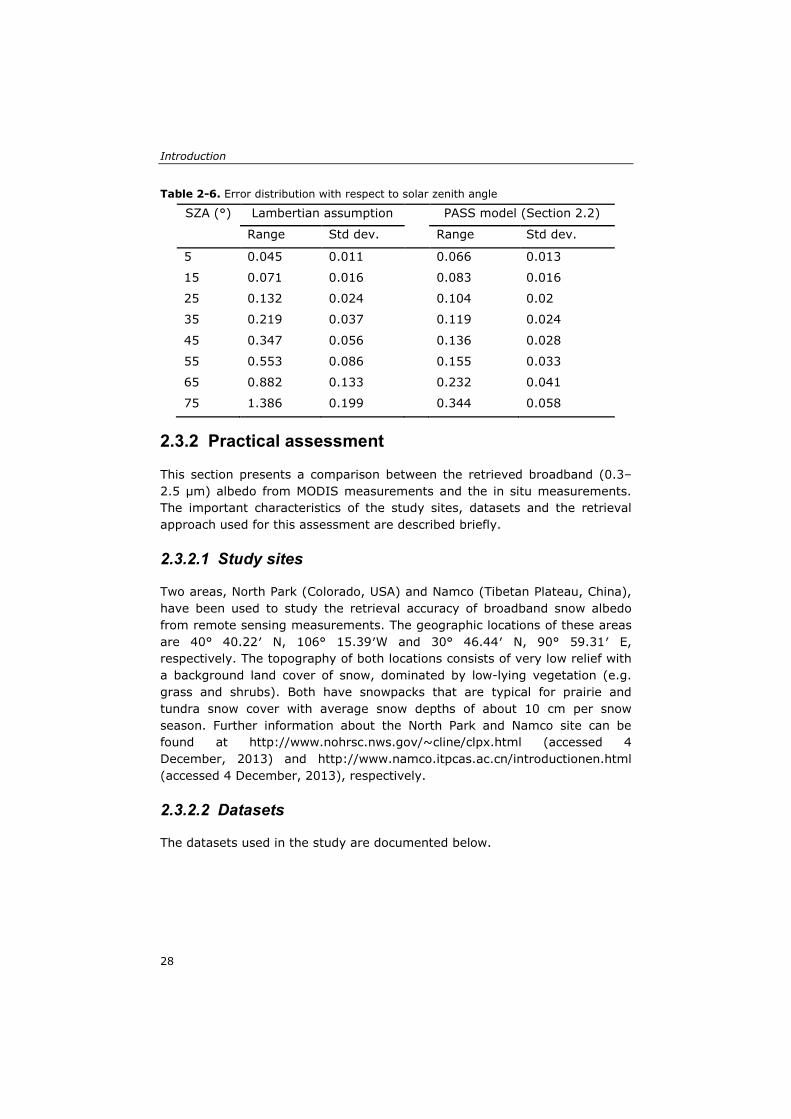
Table 2-6. Error distribution with respect to solar zenith angle .................. 28
Table 3-1. List of Landsat scenes used as ground truth ............................ 38
Table 3-2. MODTRAN specifications for the simulation ............................. 47
Table 4-1. List of the study sites along with their geographic information and snowpack conditions. Coordinates are provided in latitude and longitude using the WGS 84 geodetic system. ...................................................... 60
Table 4-2. List of instruments and respective measurements taken. a), b), and c) are for the CLPX, CDP, and Ivo sites, respectively. ........................ 63
Table 4-3. Parameter sets for four snow albedo parameterizations calibrated using measurements collected under alpine conditions during springtime snowmelt. .......................................................................................... 71
Table 4-4. List of land surface states used as model initialization and duration of model runs. .................................................................................... 73
Table 4-5. Error statistics of the Noah snow albedo simulations for the alpine sites. The temporal autocorrelation is corrected for by averaging over the correlation length of 10 days resulting in sample sizes of 48 values. .......... 75
Table 4-6. Error statistics computed between simulated and measured snow depths for the alpine sites. Temporal autocorrelation is accounted for by averaging over the correlation length of 14 days, which resulted in a sample size of 30 averaged values. .................................................................. 77
Table 4-7. Error statistics computed between measured upward shortwave radiation under alpine snow conditions and simulations with four snow albedo parameterizations. .............................................................................. 81
Table 4-8. Statistics of comparison between measured and simulated snowmelt for the CDP site. ................................................................... 82
Table 5-1. List of instruments and respective measurements taken during CLPX that are used in this study ........................................................... 93
Table 5-2. Initial states and parameters used for the NI site Noah simulations. Italic parameters are derived from NLDAS and others are obtained from the CLPX measurements. ................................................ 96
xi

Table 5-3. Error statistics of open-loop and updated snow albedo simulations for the NI site. ................................................................................... 102
Table 5-4. Error statistics of open-loop and updated snow albedo simulations for NM and NP sites ............................................................................ 106
xii
1 Introduction
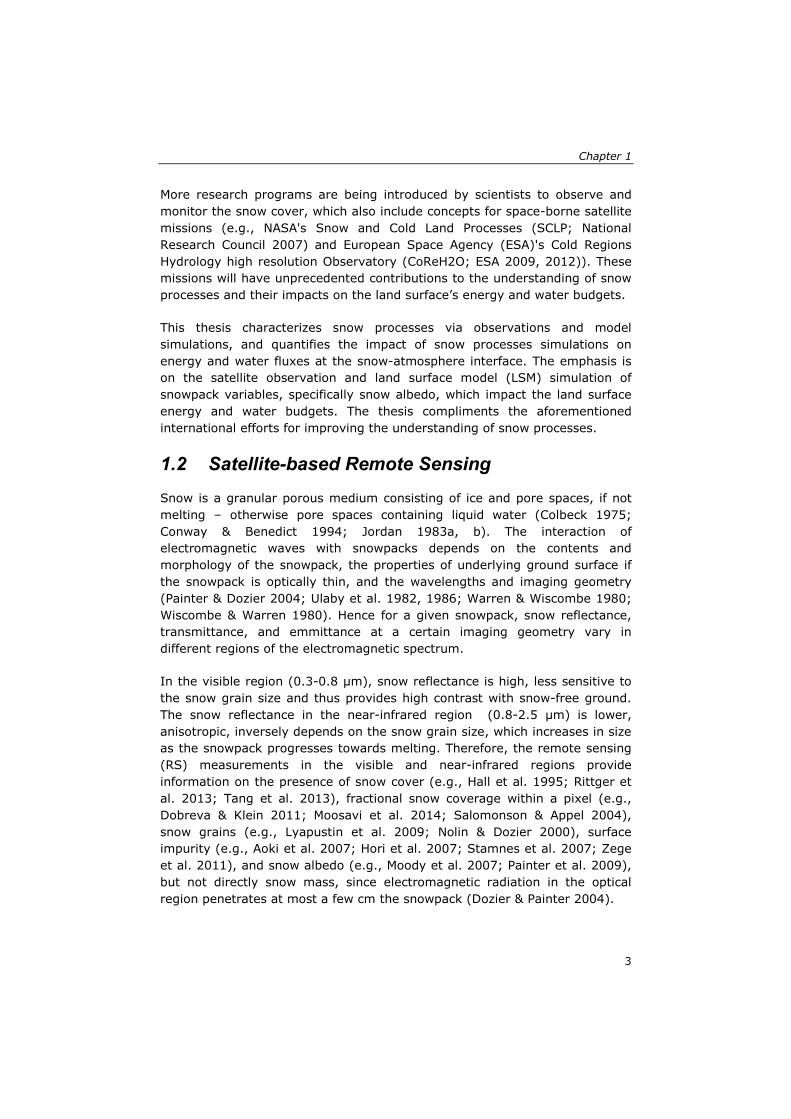
1.1 Background Snow, which acts as heat sink and freshwater source, covers nearly 50% (~ 46 x 106 km2) of the Northern Hemisphere continents during winters that reduces to 4% (~ 4 x 10⁶ km2) during summers (Frei & Robinson 1999). The variability in the Earth’s climate and weather influence the state of snow cover, making snow one of the most dynamic land covers (both in space and time) on Earth (see Figure 1-1). The snow cover state – defined by its variables, e.g., snow albedo, density, depth, coverage, and water equivalent – affects the land surface’s energy and water budgets through complex controls on the partitioning of energy and water fluxes that in turn impact the near-surface atmosphere. Snow dynamics are, therefore, important for understanding climate changes as well as the hydrological cycle.
Figure 1-1. Spatio-temporal snow cover extent on the Northern Hemisphere. 12-month average probability of occurrence for snow cover; from http://nsidc.org/data/docs/daac/nsidc0046_nh_ease_snow_seaice.gd.html
Snow albedo, snow water equivalent (SWE), and snow coverage are the variables of snow cover that affect the Earth’s energy and water cycles: the cycles which are entwined. Snow albedo defines the partitioning of incident solar radiation into radiations reflected back to the atmosphere and absorbed
1
Introduction
by the snowpack, which makes it an important variable controlling the surface energy budget. The absorbed solar radiation together with other energy fluxes (e.g., sensible and latent heat fluxes) alters the heat content (energy storage) and water equivalent (water storage) of the snowpack. Hence, snow albedo also plays a role in the water cycle by regulating the land surface’s water budget.
Snow begins to metamorphose at rates largely depend on the near-surface atmospheric dynamics soon after its deposition on the land surface (Colbeck 1983; Hachikubo & Akitaya 1997; Stössel et al. 2010). Newly formed snowpacks during winters typically transform from fine-grained (high albedo), low density, subfreezing snowpacks capable of refreezing any liquid water inputs (buffer for SWE) to coarse-grained (low albedo), isothermal at 0 °C, dense snowpacks (intimidation for SWE) that transport liquid water to the ground (Colbeck 1982; DeWalle & Rango 2008). These snowpack transformations affect at basin scale surface energy and water budgets, particularly streamflow, and thus influence the water resources management practices with in a basin.
A series of snow observation and monitoring programs has been widely implemented in the frozen landscapes for better understanding the dynamics of snow cover and exchanges of energy and water fluxes at the snow-atmosphere interface. Examples of such programs are:
• National Aeronautics and Space Administration (NASA)'s Cold Land Processes Field Experiment (CLPX) focused on developing the quantitative understanding, models, and measurements necessary to extend local-scale understanding of water fluxes, storage, and transformations to regional and global scales.
• World Climate Research Program (WCRP) supports four core projects including,
o Global Energy and Water Cycle Exchanges Project (GEWEX) focuses on the atmospheric, terestrial, radiative, hydrological, coupled processes, and interactions that determine the global and regional hydrological cycle, radiation and energy transitions, and their involvement in climate change.
o Climate and Cryosphere Program (CliC) assess and quantify the impacts of climatic variability and change on components of the cryosphere and their consequences for the climate system, and determine the stability of the global cryosphere.
2
Chapter 1
More research programs are being introduced by scientists to observe and monitor the snow cover, which also include concepts for space-borne satellite missions (e.g., NASA's Snow and Cold Land Processes (SCLP; National Research Council 2007) and European Space Agency (ESA)'s Cold Regions Hydrology high resolution Observatory (CoReH2O; ESA 2009, 2012)). These missions will have unprecedented contributions to the understanding of snow processes and their impacts on the land surface’s energy and water budgets.
This thesis characterizes snow processes via observations and model simulations, and quantifies the impact of snow processes simulations on energy and water fluxes at the snow-atmosphere interface. The emphasis is on the satellite observation and land surface model (LSM) simulation of snowpack variables, specifically snow albedo, which impact the land surface energy and water budgets. The thesis compliments the aforementioned international efforts for improving the understanding of snow processes.
1.2 Satellite-based Remote Sensing Snow is a granular porous medium consisting of ice and pore spaces, if not melting – otherwise pore spaces containing liquid water (Colbeck 1975; Conway & Benedict 1994; Jordan 1983a, b). The interaction of electromagnetic waves with snowpacks depends on the contents and morphology of the snowpack, the properties of underlying ground surface if the snowpack is optically thin, and the wavelengths and imaging geometry (Painter & Dozier 2004; Ulaby et al. 1982, 1986; Warren & Wiscombe 1980; Wiscombe & Warren 1980). Hence for a given snowpack, snow reflectance, transmittance, and emmittance at a certain imaging geometry vary in different regions of the electromagnetic spectrum.
In the visible region (0.3-0.8 µm), snow reflectance is high, less sensitive to the snow grain size and thus provides high contrast with snow-free ground. The snow reflectance in the near-infrared region (0.8-2.5 µm) is lower, anisotropic, inversely depends on the snow grain size, which increases in size as the snowpack progresses towards melting. Therefore, the remote sensing (RS) measurements in the visible and near-infrared regions provide information on the presence of snow cover (e.g., Hall et al. 1995; Rittger et al. 2013; Tang et al. 2013), fractional snow coverage within a pixel (e.g., Dobreva & Klein 2011; Moosavi et al. 2014; Salomonson & Appel 2004), snow grains (e.g., Lyapustin et al. 2009; Nolin & Dozier 2000), surface impurity (e.g., Aoki et al. 2007; Hori et al. 2007; Stamnes et al. 2007; Zege et al. 2011), and snow albedo (e.g., Moody et al. 2007; Painter et al. 2009), but not directly snow mass, since electromagnetic radiation in the optical region penetrates at most a few cm the snowpack (Dozier & Painter 2004).
3
Introduction
In contrast, passive and active microwave measurements respond directly to snow mass and thus used to retrieve SWE (e.g., Biancamaria et al. 2008; Foster et al. 1997; Hallikainen & Jolma 1992; Josberger and Mognard 2002; Kelly et al. 2003; Luojus et al. 2010; Markus et al. 2006), since at microwave wavelengths radiation penetrates dry snowpacks on the order of tens of cm to meters (Ulaby et al. 1982).
There is not a one-to-one relationship between remote sensing measurements (reflectance, brightness temperature, and backscattering) and properties of snowpack. For instance, reflectance in the visible region is sensitive to both the states of snow cover as well as the atmosphere. The sensitivity of reflectance in the visible and in the near-infrared regions is different to the changes of snow states. The effects of the imaging geometry (Bourgeois et al. 2006; Painter & Dozier 2004; Xin et al. 2012) further complicate the snow properties relationships to reflectance measurements.
The complex interaction of electromagnetic waves with temporally and spatially varying heterogeneous snowpacks challenges the retrieval of snow variables from RS observations. Therefore, a number of retrieval approaches exists for each snow cover variable based on different assumptions/approximations. Yet for a comprehensive understanding of the reliability of these retrieved estimates and their impacts on the hydrological investigations, the performance of the state-of-the-art retrieval approaches need to be intercompared for estimating the variable and improving the simulation of energy and water balance components when used within models.
1.3 Land Surface Models Land surface models (LSM) define bottom boundary conditions within numerical weather prediction and climate models by representing the energy, water, and carbon exchanges at the land-atmosphere interface. The land-atmosphere interaction depends on land surface processes that exchange energy, water, and carbon among each other. Therefore, LSMs account for various land surface processes, such as vegetation responses to environmental conditions, surface and subsurface hydrology, snowpack's evolution, and even urban, lake, and biogeochemical processes (van den Hurk et al. 2011). There are some concerns, however: How are these different processes represented? How accurate are these representations? These concerns affect simulations of energy, water, and carbon fluxes and add uncertainties to the energy, water, and carbon budget estimates of the land surface.
4
Chapter 1
To simulate energy and water fluxes at the snow surface, state-of-the-art LSMs represent various snowpack processes including snow albedo evolution, snowpack densification, liquid water retention within a snowpack, snow coverage variation in a grid-cell. These complex processes are, however, parameterized empirically rather than physically-based formulations. These parameterizations are continuously being intercomapred and/or compared with observations (e.g., Jin et al. 1999; Jin & Miller 2007; Mitchell et al. 2004; Pan et al. 2003; Sheffield et al. 2003; Slater et al. 2001; Slater et al. 2007) to better understand the snowpack processes.
Early attempts to improve cold season processes in Noah – a LSM renamed from Oregon State University (OSU) LSM, which was implemented in Eta model (now called WRF model) during 1990s – were made in an offline mode by Koren et al. (1999). These improvements include prediction of snow density (which was fixed at 0.1 g cm-3) as a function of time and snow temperature and snow fraction in a grid cell as a function of SWE. The snow thermal conductivity, which was fixed at 0.35 W-1 K-1 m-1, is affected by the change in snow density and thus the snowmelt process were more accurately simulated.
Later Ek et al. (2003) reported on improvements to Noah LSM which were most notably related to the cold season and thus to snow processes. The LSM was upgraded by geographically varying the deep snow albedo as a function of vegetation type, which was fixed to a value e.g., 0.55; accounting the snow cover patchiness effect on surface albedo of a grid cell; and including the effect of heat flow through thin patchy snow cover. In coupled evaluation, these improvements partially mitigated the cold biases (i.e., resulted in warmer 2-m air temperatures) in the winters and springs.
Recently, Livneh et al. (2010) made some revisions in snow albedo, snow aging effect, and water holding capacity of snow to improve the Noah simulation of snow processes. Barlage et al. (2010) adjusted the solar radiation for terrain slope and orientation, the surface exchange coefficient for stable boundary layers, the surface roughness length when snow is present. Further, they also confirmed the findings of Livneh et al. (2010) that time-varying snow albedo formulation is effective in improving the snowpack simulations. Very recently, Niu et al. (2011) introduced a framework called Noah-MP for multiple options to parameterize selected processes.
Although the parameterizations are continuously improving to more accurately represent snowpack processes, uncertainties still exist, which affect the energy and water fluxes’ simulations at the snowpack’s surface.
5

Introduction
1.4 Research objective The overall aim of this thesis is to improve the simulation of snow processes by LSMs, which ultimately improve energy and water fluxes simulations. To improve snow processes simulations within a LSM, we can (i) improve the model physics and/or (ii) optimally ingest RS-retrieved estimates into the LSM. The technique that allows optimal ingestion of observations of a particular variable into models to correct model predictions is known as data assimilation.
The overall aim of improving the snow process simulations is broken down into the following specific objectives:
1. To improve retrieval of snowpack’s variables – i.e., snow albedo and snow coverage – from RS.
2. To improve snowpack’s processes characterization within LSMs, in particular the snow albedo simulation.
3. To develop an assimilation scheme for ingesting the retrieved snow albedo from RS. This reduces the uncertainties inherent to snow albedo simulations.
1.5 Research questions
This study specifically seeks out to answer the following research questions:
1. Snow is highly anisotropic reflecting medium in the infrared region. How to account for the anisotropic behavior when retrieving snow albedo from RS measurements, which are acquired under different sun-sensor geometries?
2. Atmospheric perturbations and snow cover states affect the RS measurements. How can these effects be accounted for when using dual-view RS for retrieving the snow coverage within a pixel?
3. Near-snow surface atmospheric forcings control snow metamorphisms and thus the snow albedo evolution. How do existing LSM’s snow albedo parameterizations capture the evolution of measured snow seasons? What is the impact of the improved parameterization on the simulation of the surface energy and water balance?
6
Chapter 1
4. Both the LSM simulations and satellite retrievals yield uncertain estimates. Data assimilation is an approach for utilizing the satellite retrievals to obtain simulation results consistent with satellite observations. How to assimilate RS retrieved snow albedo in a LSM? How effective is the assimilation of RS retrieved snow albedo estimates in reducing uncertainties in snow albedo simulations?
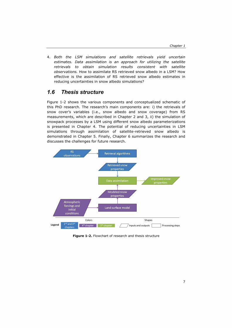
1.6 Thesis structure Figure 1-2 shows the various components and conceptualized schematic of this PhD research. The research’s main components are: i) the retrievals of snow cover’s variables (i.e., snow albedo and snow coverage) from RS measurements, which are described in Chapter 2 and 3, ii) the simulation of snowpack processes by a LSM using different snow albedo parameterizations is presented in Chapter 4. The potential of reducing uncertainties in LSM simulations through assimilation of satellite-retrieved snow albedo is demonstrated in Chapter 5. Finally, Chapter 6 summarizes the research and discusses the challenges for future research.
Figure 1-2. Flowchart of research and thesis structure
2nd and 3rd
chapters 4th chapter 5th chapter Inputs and outputs Processing steps
Colors Shapes
Legend
7

Introduction
8
2 Semi-empirical approach for estimating broadband albedo of snow
Abstract
Snow exhibits highly anisotropic and variable reflectance in the near-infrared than in the visible spectrum, challenging the development of a model that can retrieve broadband albedo from reflectance measurements. Here, a semi-empirical model is presented to estimate near-infrared (0.8–2.5 μm) albedo of snow. This model estimates spectral albedo at a wavelength of 1.240 μm using only three variables: solar zenith angle, scattering angle, and measured reflectance, which is used to retrieve near-infrared albedo. To form a base for such a model, quantification of reflectance patterns under varying snow conditions (i.e., snow grain size) and sun-sensor geometries are prerequisite. DIScrete Ordinate Radiative Transfer (DISORT) model is used to simulate bi-directional reflectance. The performance of the developed model is evaluated by using DISORT simulated spectral albedo for various snow grain sizes and solar zenith angles, as well as the Moderate Resolution Imaging Spectroradiometer (MODIS) and in situ measurements. The developed model estimates spectral albedo at 1.240 μm with acceptable – mean error, mean absolute error, and root mean squared error in the estimates are found to be 0.053, 0.055 and 0.064, respectively – and better accuracy than for those computed using the Lambertian reflectance assumption for snow, reducing the error in the range and standard deviation by 75% and 65%, respectively. Applying the model to MODIS, the retrieved albedo is found to be in strong agreement (r=0.82) with in situ measurements. These improvements in albedo estimation should allow more accurate use of remote sensing measurements in climate and hydrological models.
Based on
Malik, M. J., R. van der Velde, Z. Vekerdy, Z. Su, and M. F. Salman (2011). Semi-empirical approach for estimating broadband albedo of snow. Remote Sensing of Environment, 115(8), 2086-2095.
9
Introduction
2.1 Introduction Snow is known to have an important influence on climate and hydrological cycles at various scales. Of the properties of snow, snow albedo, snow coverage and snow water equivalent play important roles in the energy-mass balance modeling of land surfaces. To simulate and forecast weather and hydrological conditions, it is important to have estimates of these geophysical variables at the modeling scale that are as accurate as possible. Recently, Rott et al. (2009) defined the appropriate scale for snow products at a 100 to 500 m spatial resolution with a 3-day revisit time. Spatio-temporal information about snow variables at these scales not only provides a basis for initializing the models, but also helps to keep the simulations as close to reality as possible through data assimilation (Dente et al., 2008; Nagler et al., 2008). In this regard, satellite remote sensing can provide valuable information, both spatially and temporally, about the state of snow cover (Dozier et al., 2009).
Snow albedo (also referred to as hemispherical reflectivity; Schaepman-Strub et al., 2006) is a variable used in modeling that attempts to partition solar radiative fluxes at the snow-atmosphere interface. As discussed by Warren (1982), snow does not reflect uniformly in all directions, while satellite sensors only measure reflectance in certain directions. The reflectance of snow depends on sun-sensor geometry (solar zenith angle, detector's view zenith angle and the relative azimuth), snow state and wavelength. Although it is important to account for this anisotropic behavior in retrieval algorithms of spectral and broadband albedos from satellite remote sensing, the number of variables together with the changing state of snow during the season complicates the inversion procedure. That is why most of the remote sensing retrieval algorithms (Green et al., 2002; Nolin & Dozier, 2000; Painter et al., 2003, 2009) rely on the Lambertian reflectance assumption. Studies by Li et al. (2007) and Painter and Dozier (2004a) analyze the sensitivity to directional effect in the retrieval of snow properties and conclude that anisotropic behavior can lead to significant errors in retrieved snow states if the directional effect is not accounted for.
Snow is more highly absorptive in the near-infrared region of the solar spectrum than in the visible region (Warren, 1982). Thus, the near-infrared albedo plays an important role in the energy-mass balance of a snow surface (Marks & Dozier, 1992). In this study, a semi-empirical model is developed to retrieve near-infrared (0.8–2.5 μm) albedo from reflectance measurements. The objective of the study is to create a model that accounts for the anisotropic reflectance behavior of snow and that can be applied to a wide range of snow grain sizes. This study uses joint variability patterns of reflectance and spectral albedo at the wavelength of 1.240 μm to develop the
10
Chapter 2
model. These patterns are caused by the changing states of snow and sun-sensor geometry. The analysis of these variability patterns makes this method different to other methods mentioned in the literature (Klein & Stroeve, 2002; Li et al., 2007; Liang et al., 2005), which are based on the anisotropic reflectance factor (ARF) and the look up table (LUT) approach. The inherent uncertainty of the model is investigated by comparing the model-retrieved estimates with the spectral albedo calculated using DIScrete Ordinate Radiative Transfer (DISORT, Stamnes et al., 1988). The improvement in the estimates of spectral albedo, compared to those calculated using the Lambertian reflectance assumption for snow, is also quantified. Finally, results from the retrieval approach, using MODIS and in situ data from North Park (Colorado, USA — NASA Cold Land Processes Experiment) and Namco (Tibetan plateau, China) are reported.
2.2 Model description The conceptual model developed in this study is based on DISORT-simulated bi-directional reflectance (𝑅𝜆, Eq. 2.1) and the corresponding spectral albedo (𝑎𝑠,𝜆, Eq. 2.2) for varying snow grain sizes and sun-sensor geometries.
𝑅𝜆(𝜃𝑜,𝜑𝑜,𝜃𝑟 ,𝜑𝑟)[𝑠𝑟−1] = 𝐿𝜆(𝜃𝑟 ,𝜑𝑟)[𝑊 𝑚−2𝑠𝑟−1]
cos 𝜃𝑜 𝐸𝜆,𝑑𝑖𝑟[𝑊 𝑚−2] Eq. 2.1
𝑎𝑠,𝜆(𝜃𝑜)[𝑛𝑜 𝑢𝑛𝑖𝑡𝑠] = � 𝜇1
0� 𝑅𝜆2𝜋
0(𝜃𝑜,𝜑𝑜,𝜃𝑟 ,𝜑𝑟)𝑑𝜑𝑟𝑑𝜇 Eq. 2.2
Where R is bi-directional reflectance; λ is wavelength; θ, φ are the zenith and azimuth angles, respectively; subscripts o and r refer to sun and sensor, respectively; L is directional radiance;𝐸𝜆,𝑑𝑖𝑟 is the direct beam irradiance; 𝑎𝑠,𝜆 is spectral albedo; and μ is cosine of 𝜃𝑟.
The DISORT model has been used extensively to retrieve snow properties from remote sensing measurements (Liang et al., 2005; Painter et al., 2009; Stamnes et al., 2007), as well as to study bi-directional reflectance of snow (Painter & Dozier, 2004a,b). Although DISORT underestimates the hemispherical-directional reflectance factor (HDRF) in the near-infrared region of the spectrum, it is able to capture variance caused by changes in sun-sensor geometry and snow state (Painter & Dozier, 2004b). In this study, the Mie theory (Wiscombe, 1980) as well as the refractive indices of ice reported by Warren and Brandt (2008) is used to calculate single scattering properties (single scattering albedo, extinction efficiency and
11
Introduction
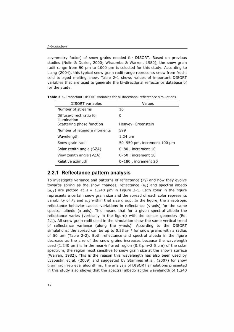
asymmetry factor) of snow grains needed for DISORT. Based on previous studies (Nolin & Dozier, 2000; Wiscombe & Warren, 1980), the snow grain radii range from 50 μm to 1000 μm is selected for this study. According to Liang (2004), this typical snow grain radii range represents snow from fresh, cold to aged melting snow. Table 2-1 shows values of important DISORT variables that are used to generate the bi-directional reflectance database of for the study.
Table 2-1. Important DISORT variables for bi-directional reflectance simulations
DISORT variables Values Number of streams 16
Diffuse/direct ratio for illumination
0
Scattering phase function Henyey–Greenstein
Number of legendre moments 599
Wavelength 1.24 μm
Snow grain radii 50–950 μm, increment 100 μm
Solar zenith angle (SZA) 0–80 , increment 10
View zenith angle (VZA) 0–60 , increment 10
Relative azimuth 0–180 , increment 20
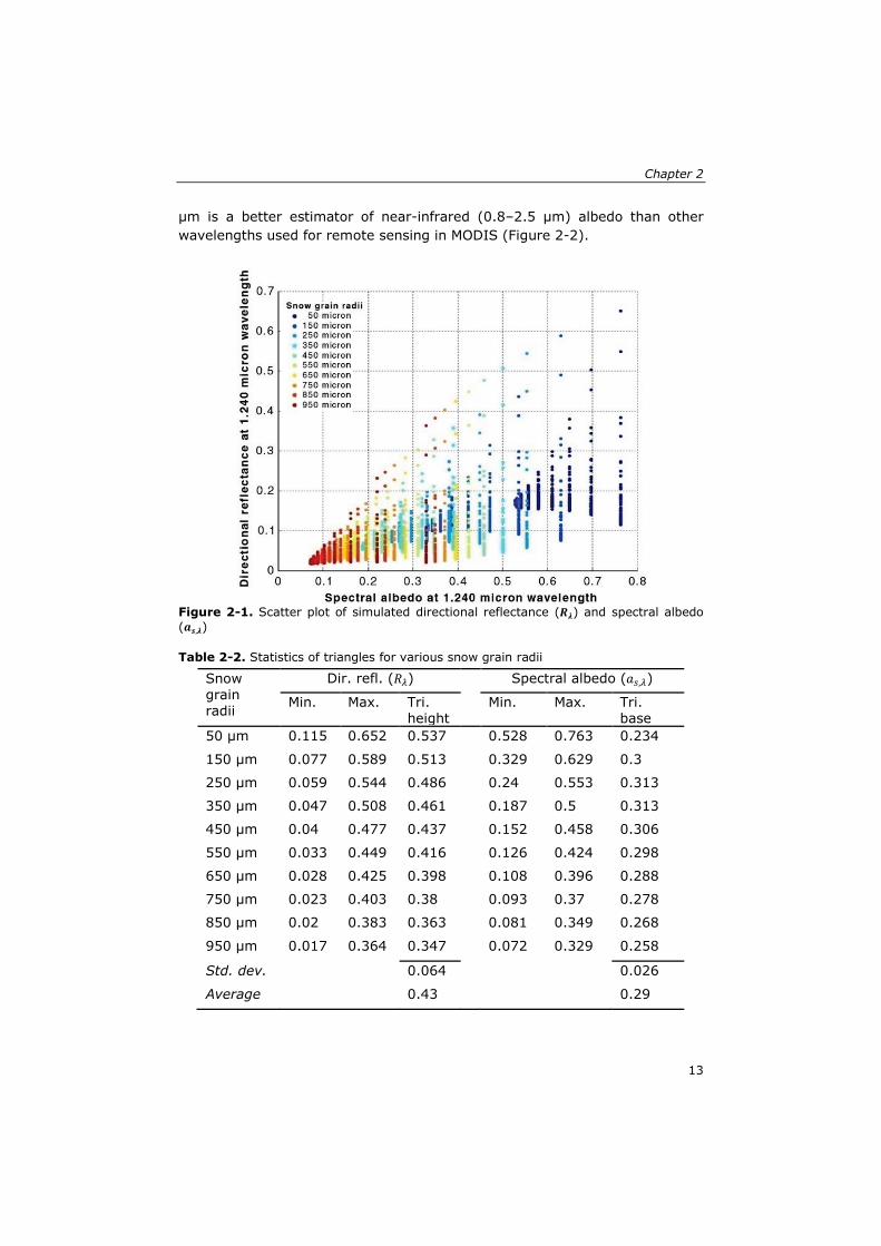
2.2.1 Reflectance pattern analysis To investigate variance and patterns of reflectance (𝑅𝜆) and how they evolve towards spring as the snow changes, reflectance (𝑅𝜆) and spectral albedo (𝑎𝑠,𝜆) are plotted at λ = 1.240 μm in Figure 2-1. Each color in the figure represents a certain snow grain size and the spread of each color represents variability of 𝑅𝜆 and 𝑎𝑠,𝜆 within that size group. In the figure, the anisotropic reflectance behavior causes variations in reflectance (y-axis) for the same spectral albedo (x-axis). This means that for a given spectral albedo the reflectance varies (vertically in the figure) with the sensor geometry (Eq. 2.1). All snow grain radii used in the simulation show the same vertical trend of reflectance variance (along the y-axis). According to the DISORT simulations, the spread can be up to 0.53 𝑠𝑟−1 for snow grains with a radius of 50 μm (Table 2-2). Both reflectance and spectral albedo in the figure decrease as the size of the snow grains increases because the wavelength used (1.240 μm) is in the near-infrared region (0.8 μm–2.5 μm) of the solar spectrum, the region most sensitive to snow grain size at the snow's surface (Warren, 1982). This is the reason this wavelength has also been used by Lyapustin et al. (2009) and suggested by Stamnes et al. (2007) for snow grain radii retrieval algorithms. The analysis of DISORT simulations presented in this study also shows that the spectral albedo at the wavelength of 1.240
12
Chapter 2
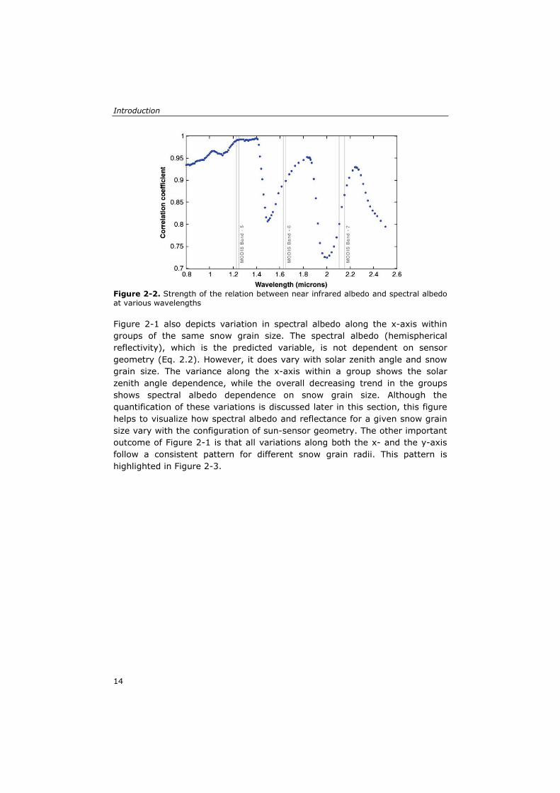
μm is a better estimator of near-infrared (0.8–2.5 μm) albedo than other wavelengths used for remote sensing in MODIS (Figure 2-2).
Figure 2-1. Scatter plot of simulated directional reflectance (𝑹𝝀) and spectral albedo (𝒂𝒔,𝝀)
Table 2-2. Statistics of triangles for various snow grain radii
Snow grain radii
Dir. refl. (𝑅𝜆) Spectral albedo (𝑎𝑠,𝜆)
Min. Max. Tri. height
Min. Max. Tri. base
50 μm 0.115 0.652 0.537 0.528 0.763 0.234
150 μm 0.077 0.589 0.513 0.329 0.629 0.3
250 μm 0.059 0.544 0.486 0.24 0.553 0.313
350 μm 0.047 0.508 0.461 0.187 0.5 0.313
450 μm 0.04 0.477 0.437 0.152 0.458 0.306
550 μm 0.033 0.449 0.416 0.126 0.424 0.298
650 μm 0.028 0.425 0.398 0.108 0.396 0.288
750 μm 0.023 0.403 0.38 0.093 0.37 0.278
850 μm 0.02 0.383 0.363 0.081 0.349 0.268
950 μm 0.017 0.364 0.347 0.072 0.329 0.258
Std. dev. 0.064 0.026
Average 0.43 0.29
13
Introduction
Figure 2-2. Strength of the relation between near infrared albedo and spectral albedo at various wavelengths
Figure 2-1 also depicts variation in spectral albedo along the x-axis within groups of the same snow grain size. The spectral albedo (hemispherical reflectivity), which is the predicted variable, is not dependent on sensor geometry (Eq. 2.2). However, it does vary with solar zenith angle and snow grain size. The variance along the x-axis within a group shows the solar zenith angle dependence, while the overall decreasing trend in the groups shows spectral albedo dependence on snow grain size. Although the quantification of these variations is discussed later in this section, this figure helps to visualize how spectral albedo and reflectance for a given snow grain size vary with the configuration of sun-sensor geometry. The other important outcome of Figure 2-1 is that all variations along both the x- and the y-axis follow a consistent pattern for different snow grain radii. This pattern is highlighted in Figure 2-3.
14
Chapter 2
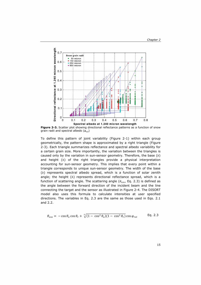
Figure 2-3. Scatter plot showing directional reflectance patterns as a function of snow grain radii and spectral albedo (𝒂𝒔,𝝀)
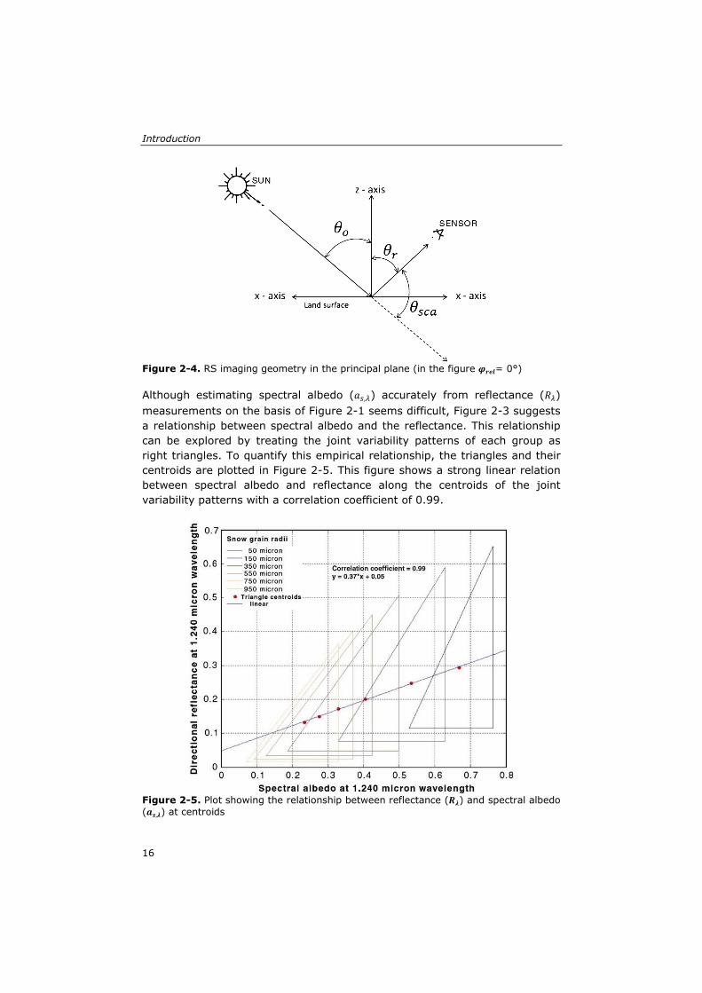
To define this pattern of joint variability (Figure 2-1) within each group geometrically, the pattern shape is approximated by a right triangle (Figure 2-3). Each triangle summarizes reflectance and spectral albedo variability for a certain grain size. More importantly, the variation between the triangles is caused only by the variation in sun-sensor geometry. Therefore, the base (𝑏) and height (ℎ) of the right triangles provide a physical interpretation accounting for sun-sensor geometry. This implies that every point within a triangle corresponds to unique sun-sensor geometry. The width of the base (𝑏) represents spectral albedo spread, which is a function of solar zenith angle; the height (ℎ) represents directional reflectance spread, which is a function of scattering angle. The scattering angle (𝜃𝑠𝑐𝑎, Eq. 2.3) is defined as the angle between the forward direction of the incident beam and the line connecting the target and the sensor as illustrated in Figure 2-4. The DISORT model also uses this formula to calculate intensities at user specified directions. The variables in Eq. 2.3 are the same as those used in Eqs. 2.1 and 2.2.
𝜃𝑠𝑐𝑎 = − cos𝜃𝑜 cos 𝜃𝑟 + �(1 − cos2 𝜃𝑜)(1 − cos2 𝜃𝑟)2 cos𝜑𝑟𝑒𝑙 Eq. 2.3
15
Introduction
Figure 2-4. RS imaging geometry in the principal plane (in the figure 𝝋𝒓𝒆𝒍= 0°)
Although estimating spectral albedo (𝑎𝑠,𝜆) accurately from reflectance (𝑅𝜆) measurements on the basis of Figure 2-1 seems difficult, Figure 2-3 suggests a relationship between spectral albedo and the reflectance. This relationship can be explored by treating the joint variability patterns of each group as right triangles. To quantify this empirical relationship, the triangles and their centroids are plotted in Figure 2-5. This figure shows a strong linear relation between spectral albedo and reflectance along the centroids of the joint variability patterns with a correlation coefficient of 0.99.
Figure 2-5. Plot showing the relationship between reflectance (𝑹𝝀) and spectral albedo (𝒂𝒔,𝝀) at centroids
16
Chapter 2
This empirical relationship opens up possibilities for the retrieval of spectral albedo from reflectance measurements. Analyzing Figure 2-1, Figure 2-2, Figure 2-3, and Figure 2-5 for different snow grain sizes and sun-sensor geometries shows that every measured reflectance is a member of a unique set of reflectance-albedo variability patterns. This pattern can be approximated by a right triangle and its centroid will be close to the regression line, as shown in Figure 2-5. With increasing snow grain size the corresponding triangular pattern and centroid will be positioned lower along the regression line. After defining the location of the centroids of the triangular patterns on the regression line, this model can estimate spectral albedo.
To retrieve spectral albedo from this empirical relationship (Figure 2-5), the dimensions for base and height of the right triangle need to be quantified. A method to locate a corresponding point within the described triangle for a given sun-sensor geometry also needs to be worked out. Then a way needs to be found to calculate reflectance at the centroid from the measured reflectance. When all these variables are known, spectral albedo of snow may be calculated using the regression model of Figure 2-5. The details of these calculations are discussed in Sections 2.2.2 and 2.2.3.
2.2.2 Geometric specifications of the triangular pattern
The base and height of the triangular pattern (Figure 2-3) represent the spectral albedo and reflectance spread, respectively (Section 2.2.1). To define these dimensions, Table 2-2 shows the range in spectral albedo and reflectance for the snow grain sizes mentioned in Table 2-1. The table shows that the base and height are not exactly the same for the different snow grain sizes. The variance (square of standard deviation) in the reflectance spread (the height) is larger than in the spectral albedo spread (the base). This is because reflectance is more sensitive to variation in the scattering angle, especially in the case of small angles, than spectral albedo is sensitive to variation in the solar zenith angle (Figure 2-6 and Figure 2-8; quantified in Figure 2-7 and Figure 2-9). This is discussed in more detail in Section 2.2.3.
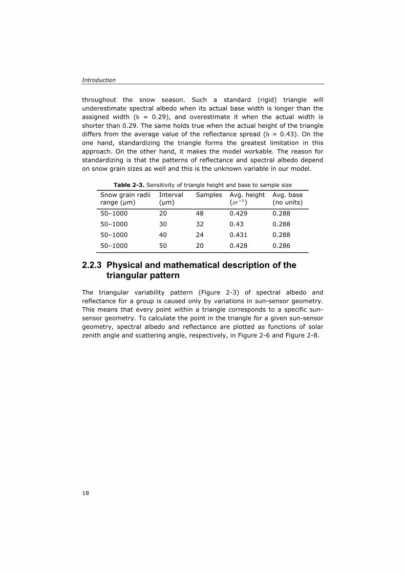
For the standard triangle the average base and height as calculated in Table 2-2 have been used, i.e. the base (b) is set at 0.29 [no units] and the height (h) at 0.43 [sr−1]. Further, to investigate the sensitivity of average base (b) and average height (h) to sample size (i.e., number of snow grain radii considered), we run DISORT simulations at snow grain radii intervals of 20, 30, 40, 50 μm. The other inputs to DISORT are kept as specified in Table 2-1. These simulations demonstrate that the b and h have limited sensitivity to sample size (see Table 2-3). This means that every pattern of joint spread (spectral albedo and reflectance) is assumed to have the same dimensions
17
Introduction
throughout the snow season. Such a standard (rigid) triangle will underestimate spectral albedo when its actual base width is longer than the assigned width (b = 0.29), and overestimate it when the actual width is shorter than 0.29. The same holds true when the actual height of the triangle differs from the average value of the reflectance spread (h = 0.43). On the one hand, standardizing the triangle forms the greatest limitation in this approach. On the other hand, it makes the model workable. The reason for standardizing is that the patterns of reflectance and spectral albedo depend on snow grain sizes as well and this is the unknown variable in our model.
Table 2-3. Sensitivity of triangle height and base to sample size
Snow grain radii range (μm)
Interval (μm)
Samples Avg. height (𝑠𝑟−1)
Avg. base (no units)
50–1000 20 48 0.429 0.288
50–1000 30 32 0.43 0.288
50–1000 40 24 0.431 0.288
50–1000 50 20 0.428 0.286
2.2.3 Physical and mathematical description of the triangular pattern
The triangular variability pattern (Figure 2-3) of spectral albedo and reflectance for a group is caused only by variations in sun-sensor geometry. This means that every point within a triangle corresponds to a specific sun-sensor geometry. To calculate the point in the triangle for a given sun-sensor geometry, spectral albedo and reflectance are plotted as functions of solar zenith angle and scattering angle, respectively, in Figure 2-6 and Figure 2-8.
18
Chapter 2
Figure 2-6. Spectral albedo as a function of solar zenith angle
Figure 2-7. Spectral albedo sensitivity with respect to solar zenith angle
Figure 2-6 depicts spectral albedo as a function of solar zenith angle for given snow grain sizes. The different colors represent the different snow grain sizes used in the simulations. The figure shows increasing trends in spectral albedo with increasing solar zenith angles for all snow grain sizes. These trends show varying sensitivity (i.e. change rate) of the spectral albedo to changes in the solar zenith angle. Sensitivity increases as the solar zenith angle
19
Introduction
increases. This qualitative analysis helps understand how a point along the base of the triangle will move from left to right as the solar zenith angle changes from 0 to 80° (Figure 2-10).
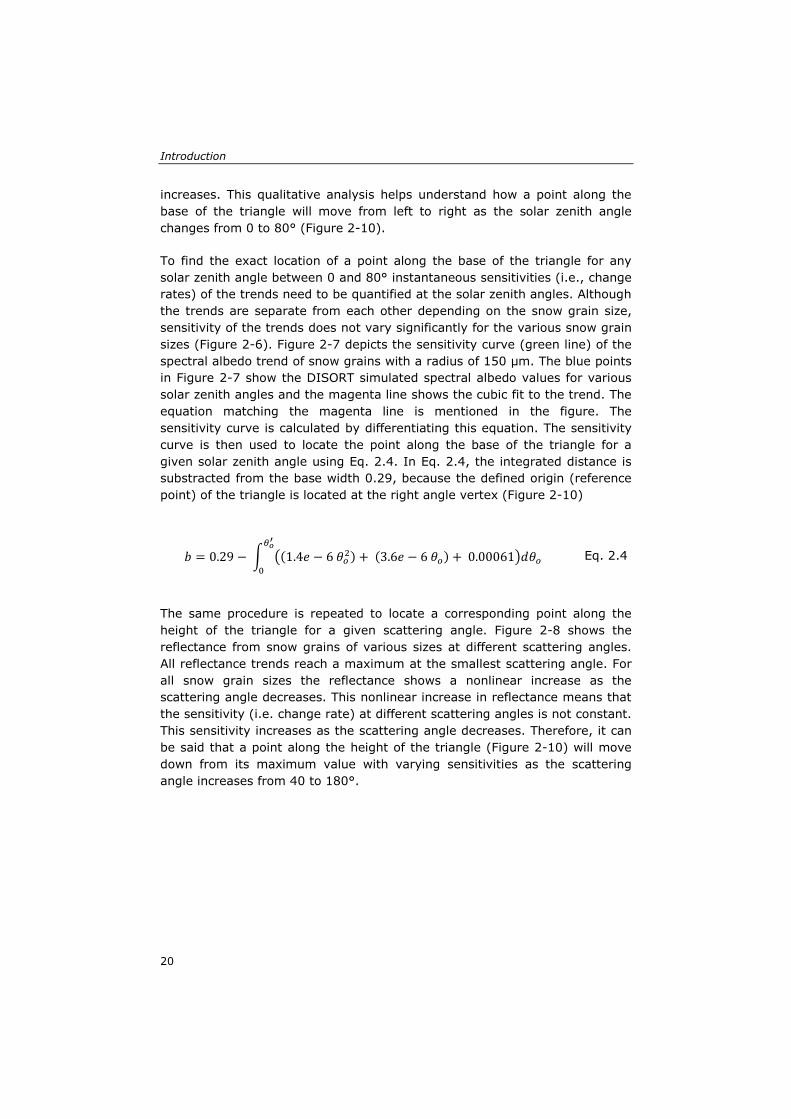
To find the exact location of a point along the base of the triangle for any solar zenith angle between 0 and 80° instantaneous sensitivities (i.e., change rates) of the trends need to be quantified at the solar zenith angles. Although the trends are separate from each other depending on the snow grain size, sensitivity of the trends does not vary significantly for the various snow grain sizes (Figure 2-6). Figure 2-7 depicts the sensitivity curve (green line) of the spectral albedo trend of snow grains with a radius of 150 μm. The blue points in Figure 2-7 show the DISORT simulated spectral albedo values for various solar zenith angles and the magenta line shows the cubic fit to the trend. The equation matching the magenta line is mentioned in the figure. The sensitivity curve is calculated by differentiating this equation. The sensitivity curve is then used to locate the point along the base of the triangle for a given solar zenith angle using Eq. 2.4. In Eq. 2.4, the integrated distance is substracted from the base width 0.29, because the defined origin (reference point) of the triangle is located at the right angle vertex (Figure 2-10)
𝑏 = 0.29 − � �(1.4𝑒 − 6 𝜃𝑜2) + (3.6𝑒 − 6 𝜃𝑜) + 0.00061�𝑑𝜃𝑜𝜃𝑜′
0 Eq. 2.4
The same procedure is repeated to locate a corresponding point along the height of the triangle for a given scattering angle. Figure 2-8 shows the reflectance from snow grains of various sizes at different scattering angles. All reflectance trends reach a maximum at the smallest scattering angle. For all snow grain sizes the reflectance shows a nonlinear increase as the scattering angle decreases. This nonlinear increase in reflectance means that the sensitivity (i.e. change rate) at different scattering angles is not constant. This sensitivity increases as the scattering angle decreases. Therefore, it can be said that a point along the height of the triangle (Figure 2-10) will move down from its maximum value with varying sensitivities as the scattering angle increases from 40 to 180°.
20
Chapter 2
Figure 2-8. Reflectance as function of scattering angle
Figure 2-9. Reflectance sensitivity with respect to scattering angle
Figure 2-9 depicts the sensitivity curve (green line) of the forth degree fit (yellow line) to the reflectance trend of snow grains with a 150 micron radius. This sensitivity curve is used in Eq. 2.5 to locate a corresponding point on the triangle's height for a given scattering angle. The integral part of Eq. 2.5 is subtracted from the average height of 0.43 [sr−1], because the origin of the triangle is located at the right angle vertex (Figure 2-10).
21
Introduction
ℎ = 0.43 − � ((−1.9𝑒 − 8 𝜃𝑠𝑐𝑎3 ) + (7.9𝑒 − 6 𝜃𝑠𝑐𝑎2 ) − (0.0011 𝜃𝑠𝑐𝑎)𝜃𝑠𝑐𝑎′
40+ 0.05) 𝑑𝜃𝑠𝑐𝑎
Eq. 2.5
Figure 2-10. Geometry of the triangular pattern of approximate joint variability of 𝑹𝝀 and 𝒂𝒔,𝝀
All the variables needed for the empirical model (Figure 2-5), as discussed in the last paragraph of Section 2.2.1 , have now been quantified. Figure 2-10 shows the complete geometrical description of the triangle that approximates the pattern of joint variability (spectral albedo and reflectance) discussed in Section 2.2.1. The coordinates of the centroid of the triangle are (0.10, 0.14), based on the origin (0, 0) being at the right angle vertex. Now spectral albedo (as,λ; λ = 1.240 μm) may be calculated for a given reflectance (Rλ; λ = 1.240 μm) measured at a specific configuration of sun-sensor geometry.
2.3 Results and discussion Before applying the retrieval approach on actual measurements by space-borne remote sensors, intrinsic uncertainties in spectral albedo estimation induced in the approach are quantified because of the assumptions discussed in Section 2.2. Section 2.3.1 gives a comparison between the retrieved spectral albedo of the presented approach (hereafter referred to as PAttern-BasSd Semi-empirical (PASS)) and the DISORT simulated spectral albedo.
22
Chapter 2
Quantification of the improvement in the estimates in relation to the Lambertian assumption for snow reflectance is also presented. Section 2.3.2 discusses the results of retrieved broadband albedo from MODIS using the proposed approach.
2.3.1 Theoretical assessment
This section is divided into two parts. In the first part the performance of the model is analyzed, while the second part shows how the error (or residuals) distribution varies with snow grain size and sun-sensor geometry. We acknowledge that this assessment has limitation in the sense that the same theoretical model is used for both development and the assessment. However, the purpose of this section is to understand the scenarios that cause errors in the estimatesthat are inherent to our approach.
To assess the accuracy of the approach discussed in Section 2.2, another set of DISORT simulation variables is used. This set uses different snow grain sizes and solar zenith angles than the ones used in Table 2-1 for the model development. Table 2-4 shows set of variables defining the assessment scenario.
Table 2-4. DISORT variables for validation scenario
DISORT variables Values Number of streams 16
Diffuse/direct ratio for illumination 0
Scattering phase function Henyey–Greenstein
Number of legendre moments 599
Wavelength 1.24 μm
Snow grain radii 100–1000 μm, increment 100 μm
Solar zenith angle (SZA) 5–75°, increment 10°
View zenith angle (VZA) 0–60°, increment 10°
Relative azimuth 0–180°, increment 20°
2.3.1.1 Model performance
Figure 2-11 shows the scatter plot of DISORT albedo and empirically calculated spectral albedo using the PASS method of Section 2.2. The figure shows a significantly improved spread of points along the 1:1 line compared to Figure 2-1 (if Rλ multiplied by π i.e. Lambertian assumption for spectral albedo). The correlation coefficient of the spread is found to be 0.926. The linearity and squeezed spread in the figure show that the developed model is
23
Introduction
able to calculate spectral albedo with reasonable accuracy for a given reflectance measurement at a known configuration of sun-sensor geometry. The colors in the figure depict different snow grain sizes, corresponding to various snow surface conditions from fine new snow to coarse melting snow. The spread of each color is consistent along the 1:1 line. This implies that the performance of the model does not vary much with snow grain size, which gives confidence when applying this model rather than the Lambertian assumption to spectral albedo calculation. Further assessment of the model is quantified in Table 2-5 and Figure 2-12, which present the statistics of the residuals.
Table 2-5. Quantification of the model performance in comparison to Lambertian assumption
Lambertian assumption
PASS (Section 2.2)
ME −0.036 0.053
Error range 1.386 0.343
Std dev. 0.103 0.036
MAE 0.068 0.055
RMSE 0.109 0.064
Figure 2-11. Comparison of DISORT albedo and empirically retrieved albedo
24
Chapter 2
Figure 2-12. Comparison of error distributions
Table 2-5 shows that the PASS approach developed in Section 2.2 has a tendency to overestimate spectral albedo with a positive mean error (ME). This is also visualized in Figure 2-11. Most of the points in the figure are above the 1:1-line. The standard error in the predicted estimates is 0.055. This means that on average the model has a ± 0.055 error in its estimated values. These estimated values show only slight improvement over the values obtained through Lambertian assumption, but the error range, standard deviation of errors and root mean square error (RMSE) show a significant reduction in error distribution compared to those obtained through Lambertian assumption. Figure 2-12 shows a comparison between error distributions for the Lambertian case and the empirical approach (Section 2.2). Analysis shows that the range and standard deviation of errors are reduced by 75% and 65%, respectively. In view of these results, it can be said that the model overestimates spectral albedo with an average error of ± 0.055 but that this error would remain between − 0.144 and 0.199 (i.e., error range = 0.343; see Figure 2-12). This is quite a significant improvement over the Lambertian assumption, where the error can vary from − 0.315 to 1.071 (i.e., error range = 1.386; see Figure 2-12).
2.3.1.2 Error distribution
Section 2.3.1.1 discussed that the model in general overestimates spectral albedo (Figure 2-11), but is quite effective in reducing the spread of error distribution (Figure 2-12). The other remark made in Section 2.3.1.1 is that
25
Introduction
the model's performance does not vary largely with snow grain sizes. This is more explicitly visualized in Figure 2-13, which shows the error distribution as a function of snow grain size. Although the peak of the distributions is shifting upwards as the snow gets coarser, the overall distributions are not showing a distinctive relationship with snow grain size. Consequently, the error distributions of different snow grain sizes are not separable. This implies that the same absolute error in estimated spectral albedo holds for fine grained snow as well as for coarse grained snow. From a relative perspective, however, coarse grained snow surface has a lower spectral albedo and will, thus, with the same error distribution be subject to larger uncertainties.
Figure 2-13. Error distributions for various snow grain sizes
Figure 2-13 shows that the error distributions, at least in an absolute sense, have no significant dependence on snow grain sizes. To explore the influence of sun-sensor geometry on error distribution, Figure 2-14 shows errors as a function of solar zenith angle and scattering angle. By comparing Figure 2-13 with Figure 2-14, the cause of variation in error shown in Figure 2-13 may be understood. For clarity, the error statistics in Figure 2-14 are only plotted for 100, 500 and 1000 μm snow grain sizes. Figure 2-14 shows that the maximum error variation for all three snow grain radii occurs at the highest solar zenith angle. This implies that the range of error distributions (Figure 2-13) depends on the error variation at the 80 degree solar zenith angle. Figure 2-14 also shows the effect on the estimates of rigid triangular approximation to joint variability patterns (Section 2.2.2). As discussed in
26
Chapter 2
Section 2.2.2, this approximation would induce uncertainties in the estimates. The error trend in Figure 2-14 is in accordance with Table 2-2. Figure 2-14 shows that in general the spectral albedo of coarse grains is overestimated because the width of the base of the triangle is greater than the actual base of the triangular pattern. However, the figure also shows underestimation for coarse snow at smaller scattering angles. This is caused by the average length being greater than the actual length of triangular pattern.
Table 2-6 shows the range and standard deviation of the error distribution, obtained with both the Lambertian and semi-empirical approaches, for all snow grain sizes and scattering angles used in this assessment as a function of the solar zenith angle (SZA). The statistics demonstrate that the semi-empirical approach performs better than the Lambertian approach from a SZA of 25°. Lambertian approach produces more accurate results at lower SZA. However, the snow dominated regions are situated near the mid and high latitude regions (Barnett et al., 2005), where the SZAs are typically higher than 25°, especially during winters. On the hand, in high altitude regions near the mid-latitudes (e.g., Tibetan Plateau) snow may occur during the summer. Under those circumstances the Lambertian approach performs better.
Figure 2-14. Error distributions as function of solar zenith angle and scattering angle
27
Introduction
Table 2-6. Error distribution with respect to solar zenith angle
SZA (°) Lambertian assumption PASS model (Section 2.2)
Range Std dev. Range Std dev.
5 0.045 0.011 0.066 0.013
15 0.071 0.016 0.083 0.016
25 0.132 0.024 0.104 0.02
35 0.219 0.037 0.119 0.024
45 0.347 0.056 0.136 0.028
55 0.553 0.086 0.155 0.033
65 0.882 0.133 0.232 0.041
75 1.386 0.199 0.344 0.058
2.3.2 Practical assessment
This section presents a comparison between the retrieved broadband (0.3–2.5 μm) albedo from MODIS measurements and the in situ measurements. The important characteristics of the study sites, datasets and the retrieval approach used for this assessment are described briefly.
2.3.2.1 Study sites
Two areas, North Park (Colorado, USA) and Namco (Tibetan Plateau, China), have been used to study the retrieval accuracy of broadband snow albedo from remote sensing measurements. The geographic locations of these areas are 40° 40.22′ N, 106° 15.39′W and 30° 46.44′ N, 90° 59.31′ E, respectively. The topography of both locations consists of very low relief with a background land cover of snow, dominated by low-lying vegetation (e.g. grass and shrubs). Both have snowpacks that are typical for prairie and tundra snow cover with average snow depths of about 10 cm per snow season. Further information about the North Park and Namco site can be found at http://www.nohrsc.nws.gov/~cline/clpx.html (accessed 4 December, 2013) and http://www.namco.itpcas.ac.cn/introductionen.html (accessed 4 December, 2013), respectively.
2.3.2.2 Datasets
The datasets used in the study are documented below.
28
Chapter 2
2.3.2.2.1 In situ measurements
Two sets of meteorological measurements of upwelling and downwelling solar fluxes are used for the assessment of the retrieval approach. These components of solar radiation are used to calculate broadband albedo of snow surface, which is then compared with the retrieved estimates of albedo from remote sensing data. One set of measurements was collected between 20th September, 2002, and 1st October, 2003, at three sites in North Park, namely Potter Creek, Illinois River, and Michigan River (Elder & Goodbody, 2004). At these sites the temporal resolution of the measurements was 10 min. The other set of measurements was collected at Namco weather station between 1st November, 2006 and 31st December, 2006. The measurements at this weather station were recorded at a 30 minute temporal resolution. The stations in both the United States and China were equipped with the Kipp and Zonen CNR1 Net Radiometer, which measures the up- and downwelling shortwave radiation in the 0.3–2.8 wavelength range with a reported accuracy of +/−10% (Elder et al., 2009; Ma et al., 2009). For comparison with the retrieved estimates of albedo from MODIS, average values of albedo are used for the time period of a satellite overpass (approximately 2 h).
2.3.2.2.2 MODIS product used for the retrieval
To retrieve the spectral albedo of snow, the PASS approach presented in Section 2.2 requires information about sun zenith angle, sensor zenith angle, relative azimuth between sun and sensor, and the measured reflectance at the wavelength of 1.240 μm. To parameterize these variables, the MOD02HKM MODIS product was used along with the information regarding the sun-sensor geometry. MOD02HKM is a level 1B product from the TERRA satellite. It gives calibrated and geolocated top-of-the atmosphere (TOA) radiance in units of W/(m2 μm sr) at a spatial resolution of 500 m. Based on the information in the metadata of MOD02HKM, the radiance in band 5 (1.230–1.250 μm) is converted to reflectance in units ofsr−1. Although the approach requires at-snow-surface reflectance measurements, TOA reflectance measurements were used, because MODIS atmospheric corrections are primarily suited to dense vegetation (Liang et al., 2005; Tedesco & Kokhanovsky, 2007). The study by Tedesco and Kokhanovsky (2007) also shows that error in retrievals due to atmospheric corrections can vary ± 40% depending on snow grain size. Therefore, in this preliminary investigation TOA reflectance measurements are sufficient to assess the potentials of the approach. Further information about the product can be found athttp://mcst.gsfc.nasa.gov/uploads/files/M1054.pdf (accessed 4 December, 2013).
29
Introduction
2.3.2.3 Broadband snow albedo retrieval
In order to compare MODIS retrieved broadband albedo with the in situ measurements, the relationship between the spectral albedo at the wavelength of 1.240 μm and the near-infrared albedo (0.8–2.5 μm) needs to be defined, as well as the way to integrate the visible albedo (0.4–0.8 μm) with the near-infrared albedo (0.8–2.5 μm).
Figure 2-15 shows the relationship between the DISORT simulated spectral albedo at the 1.240 μm wavelength and the near-infrared albedo (0.8–2.5 μm) for the snow grain sizes and sun-sensor geometries mentioned in Table 2-1 and Table 2-4. The figure also shows the residual plot of linear, quadratic and cubic models fitted to the simulated data. The non-linearity of the relationship at high albedo values causes linear and quadratic models to underestimate near-infrared albedo from spectral albedo at the wavelength of 1.240 μm. For this reason, linear and quadratic models have large residuals at high albedo values in comparison to cubic fit models. In brief, the plot suggests that the albedo of the near-infrared region, which is sensitive primarily to snow grain size at the surface and has limited penetration depth, can be estimated quite accurately from spectral albedo estimates of the same wavelength. For this study, therefore, the cubic model was used to estimate near-infrared albedo.
30
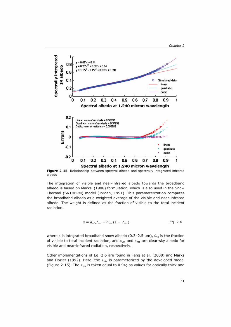
Chapter 2
Figure 2-15. Relationship between spectral albedo and spectrally integrated infrared albedo
The integration of visible and near-infrared albedo towards the broadband albedo is based on Marks' (1988) formulation, which is also used in the Snow Thermal (SNTHERM) model (Jordan, 1991). This parameterization computes the broadband albedo as a weighted average of the visible and near-infrared albedo. The weight is defined as the fraction of visible to the total incident radiation.
𝑎 = 𝑎𝑣𝑖𝑠𝑓𝑣𝑖𝑠 + 𝑎𝑛𝑖𝑟(1 − 𝑓𝑣𝑖𝑠) Eq. 2.6
where a is integrated broadband snow albedo (0.3–2.5 μm), fvis is the fraction of visible to total incident radiation, and avis and anir are clear-sky albedo for visible and near-infrared radiation, respectively.
Other implementations of Eq. 2.6 are found in Feng et al. (2008) and Marks and Dozier (1992). Here, the anir is parameterized by the developed model (Figure 2-15). The avis is taken equal to 0.94; as values for optically thick and
31
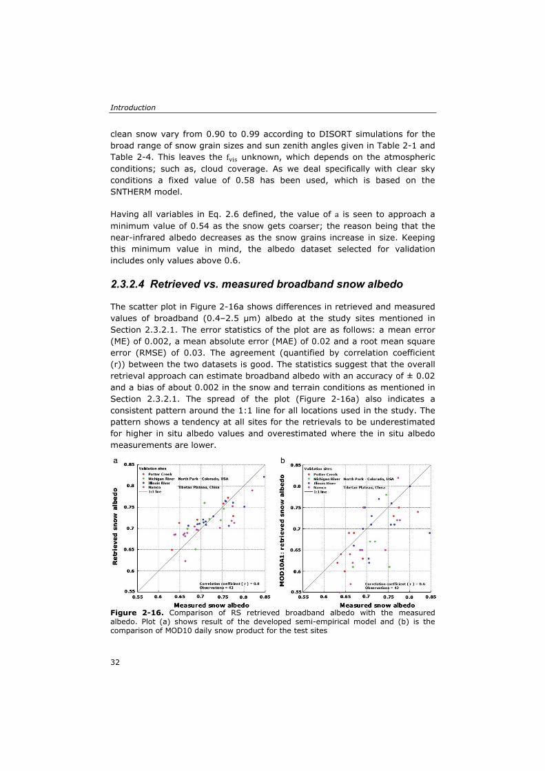
Introduction
clean snow vary from 0.90 to 0.99 according to DISORT simulations for the broad range of snow grain sizes and sun zenith angles given in Table 2-1 and Table 2-4. This leaves the fvis unknown, which depends on the atmospheric conditions; such as, cloud coverage. As we deal specifically with clear sky conditions a fixed value of 0.58 has been used, which is based on the SNTHERM model.
Having all variables in Eq. 2.6 defined, the value of a is seen to approach a minimum value of 0.54 as the snow gets coarser; the reason being that the near-infrared albedo decreases as the snow grains increase in size. Keeping this minimum value in mind, the albedo dataset selected for validation includes only values above 0.6.
2.3.2.4 Retrieved vs. measured broadband snow albedo
The scatter plot in Figure 2-16a shows differences in retrieved and measured values of broadband (0.4–2.5 μm) albedo at the study sites mentioned in Section 2.3.2.1. The error statistics of the plot are as follows: a mean error (ME) of 0.002, a mean absolute error (MAE) of 0.02 and a root mean square error (RMSE) of 0.03. The agreement (quantified by correlation coefficient (r)) between the two datasets is good. The statistics suggest that the overall retrieval approach can estimate broadband albedo with an accuracy of ± 0.02 and a bias of about 0.002 in the snow and terrain conditions as mentioned in Section 2.3.2.1. The spread of the plot (Figure 2-16a) also indicates a consistent pattern around the 1:1 line for all locations used in the study. The pattern shows a tendency at all sites for the retrievals to be underestimated for higher in situ albedo values and overestimated where the in situ albedo measurements are lower.
Figure 2-16. Comparison of RS retrieved broadband albedo with the measured albedo. Plot (a) shows result of the developed semi-empirical model and (b) is the comparison of MOD10 daily snow product for the test sites
32
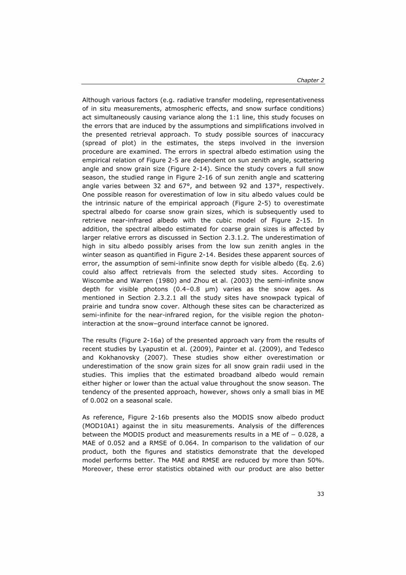
Chapter 2
Although various factors (e.g. radiative transfer modeling, representativeness of in situ measurements, atmospheric effects, and snow surface conditions) act simultaneously causing variance along the 1:1 line, this study focuses on the errors that are induced by the assumptions and simplifications involved in the presented retrieval approach. To study possible sources of inaccuracy (spread of plot) in the estimates, the steps involved in the inversion procedure are examined. The errors in spectral albedo estimation using the empirical relation of Figure 2-5 are dependent on sun zenith angle, scattering angle and snow grain size (Figure 2-14). Since the study covers a full snow season, the studied range in Figure 2-16 of sun zenith angle and scattering angle varies between 32 and 67°, and between 92 and 137°, respectively. One possible reason for overestimation of low in situ albedo values could be the intrinsic nature of the empirical approach (Figure 2-5) to overestimate spectral albedo for coarse snow grain sizes, which is subsequently used to retrieve near-infrared albedo with the cubic model of Figure 2-15. In addition, the spectral albedo estimated for coarse grain sizes is affected by larger relative errors as discussed in Section 2.3.1.2. The underestimation of high in situ albedo possibly arises from the low sun zenith angles in the winter season as quantified in Figure 2-14. Besides these apparent sources of error, the assumption of semi-infinite snow depth for visible albedo (Eq. 2.6) could also affect retrievals from the selected study sites. According to Wiscombe and Warren (1980) and Zhou et al. (2003) the semi-infinite snow depth for visible photons (0.4–0.8 μm) varies as the snow ages. As mentioned in Section 2.3.2.1 all the study sites have snowpack typical of prairie and tundra snow cover. Although these sites can be characterized as semi-infinite for the near-infrared region, for the visible region the photon-interaction at the snow–ground interface cannot be ignored.
The results (Figure 2-16a) of the presented approach vary from the results of recent studies by Lyapustin et al. (2009), Painter et al. (2009), and Tedesco and Kokhanovsky (2007). These studies show either overestimation or underestimation of the snow grain sizes for all snow grain radii used in the studies. This implies that the estimated broadband albedo would remain either higher or lower than the actual value throughout the snow season. The tendency of the presented approach, however, shows only a small bias in ME of 0.002 on a seasonal scale.
As reference, Figure 2-16b presents also the MODIS snow albedo product (MOD10A1) against the in situ measurements. Analysis of the differences between the MODIS product and measurements results in a ME of − 0.028, a MAE of 0.052 and a RMSE of 0.064. In comparison to the validation of our product, both the figures and statistics demonstrate that the developed model performs better. The MAE and RMSE are reduced by more than 50%. Moreover, these error statistics obtained with our product are also better
33
Introduction
than the ones found in previous studies (Stroeve et al., 2005, 2006 and Wang & Zender, 2010). Through data assimilation, such improved snow albedo estimation can contribute to a reduction of uncertainties in the simulation of land surface processes in snow covered regions.
2.4 Conclusion In this chapter, a Pattern-Based Semi-empirical (PASS) model to estimate near-infrared (0.8–2.5 μm) albedo of snow from directional reflectance measurements is described. This model accounts for anisotropic reflectance behavior of snow and can be applied in varying snow surface conditions i.e. snow grain sizes. The model is based on the linear empirical relation between reflectance and spectral albedo at the wavelength of 1.240 μm for various snow grain sizes. This relation has been explored by treating the patterns of joint variability as a right triangle. Each triangular pattern accounts for the variance caused in reflectance and albedo by changing the sun-sensor geometry. The retrieved spectral albedo at 1.240 μm wavelength (corrected for anisotropic effects) is then used to estimate near-infrared albedo. The performance of the model has been evaluated for a wide range of sun-sensor geometries and snow surface conditions using both simulated and real datasets. The validation results using simulated datasets show the model in general overestimates the spectral albedo with an average error of about 0.055. The performance of the model is consistent for varying snow surface conditions. The results also show a significant reduction in error distribution compared to the Lambertian assumption for snow reflectance. The retrieval model has also been applied to the MODIS sensor. The results show that the model tends to overestimate the broadband albedo of coarse grained snow and underestimate the albedo of fine grained snow. However, overall comparison of the MODIS retrieved estimates with the in situ measurements shows good agreement (r = 0.82) between the datasets with a mean error of 0.002 on a seasonal scale. The improved estimates of near-infrared albedo should allow more accurate albedo parameterization of snow cover from remote sensing measurements for climate and hydrological modeling. In brief, this approach is simple, reasonably accurate, computationally efficient and easy to implement because it only requires information about directional reflectance acquired at specific sun-sensor geometry.
The proposed model is developed for retrieving the near-infrared albedo from RS measurements and, as such, provides a better estimate of the broadband albedo (0.3–2.5 μm) of snow as compared to the available MODIS product (i.e., MOD10A1). Further enhancement of the remotely sensed broadband albedo could be achieved via the visible albedo. The visible albedo of snow is most sensitive to impurity contents and is also a function of the atmospheric visibility (i.e., aerosols type and concentration).
34
3 Prospects of dual view remote sensing for fractional snow cover mapping
Abstract
Snow coverage, an important variable of the Earth, governs thermodynamic state of the land surface. This study has two objectives related to fractional snow cover (FSC) mapping at moderate spatial resolutions from remote sensing (RS) data: i) to quantify the performance of the existing FSC mapping algorithm and ii) to assess potentials of dual-view RS for the mapping. The FSC estimation algorithm used in the daily MODIS snow product is evaluated by using simulated and Landsat TM/ETM+ data over the North Park (Colorado, USA). Simulations suggest that the algorithm besides FSC is also sensitive to snow grain size, sun sensor geometry, and background land surface state, which induce uncertainties up to ± 20% in the FSC estimates. The comparison of MODIS FSC estimates with the Landsat data shows that the MODIS FSC estimates are uncertain up to ±35%, with a weak correlation (R2 = 0.45) between the datasets. The possible reasons for this increased (compared to simulations) uncertainty could be atmospheric variations – because the algorithm uses top-of-atmosphere reflectance measurements – and reflectance contrast variations between background land surface and snow in the wavelength band centered at 1640 nm (i.e., MODIS band 6). In comparison to the MODIS algorithm, MODTRAN simulations show that the dual viewing provides a way – relative contrast difference between the two views – for accounting for the atmospheric effects on the retrieved FSC estimates using the visible bands and hence reduces the uncertainty up to 20% in the estimates.
Based on
Malik, M. J., R. van der Velde, Z. Vekerdy, and Z. Su. Prospects of dual view remote sensing for fractional snow cover mapping. In preparation for submission.
35
Prospects of dual view remote sensing for fractional snow cover mapping
3.1 Introduction Snow is a land cover (also considered as a blanket covering the land surface during winters) that is most reflective in the visible region for incoming solar radiation, sensitive to climate and weather variations, and important reservoir of fresh water. Along with glaciers, seasonal snow cover is a source of water supply for more than one-sixth of the Earth's population (Barnett et al., 2005). To study the effects of climate change on snow cover dynamics and manage water resources in snow-dominated river basins, remote sensing (RS) can provide information about various variables of snow cover (e.g., snow cover extents, snow albedo, snow grain, snow wetness, etc.). Therefore, these RS retrieved estimates are extensively used to parameterize and validate different land surface and hydrological models (e.g., Immerzeel et al., 2010; Tekeli et al., 2005). Further, uncertainty estimates of the RS retrieved variables also become important for optimum ingestion of the retrieved variable in model simulations using data assimilations techniques to improve forecasts (Reichle, 2008).
As snow states are quite dynamic in time and cloud cover also obstructs optical RS measurements, moderate spatial resolution remote sensors (ranging from 500 m) with their high temporal resolution are normally used for studying spatio-temporal variations in snow cover properties. The Sentinel-3 mission – a constellation of two satellites and a multi-instrument mission – will allow higher temporal sampling/observation frequency of seasonal snow cover through its stringent revisit time and swath coverage. The optical sensors onboard the satellites (i.e., the Ocean Land Colour Instrument (OLCI) and the Sea Land Surface Temperature Radiometer (SLSTR)) have spectral bands that are important for snow cover monitoring. For instance, SLSTR’s visible bands centered at 550 nm and 660 nm can be used for snow cover mapping, and shortwave infrared bands centered at 1375 nm and 1610 nm can be used for snow-cloud discrimination.
The challenge in RS is the inversion of the measured signals in different spectral bands to retrieve estimates of physical variables of the Earth-atmosphere system. Normally, RS retrieved estimates of the variables from large scale measurements always have some uncertainties/inaccuracies. Because, the measured signal is a mixture of contributions from the atmosphere, from different land cover compositions (i.e., snow and non-snow covered fractions), and their states. The unmixing of the measurements is usually done with the help of some approximations and empirical relations (Kaufman et al., 2002; Levy et al., 2007; Salomonson & Appel, 2004). Insights into the uncertainty of these empirical relations/algorithms allow more intelligent use of the retrieved estimates for modeling snow cover properties under different climate/weather and physiographic conditions.
36
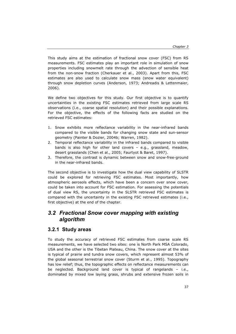
Chapter 3
This study aims at the estimation of fractional snow cover (FSC) from RS measurements. FSC estimates play an important role in simulation of snow properties including snowmelt rate through the advection of sensible heat from the non-snow fraction (Cherkauer et al., 2003). Apart from this, FSC estimates are also used to calculate snow mass (snow water equivalent) through snow depletion curves (Anderson, 1973; Andreadis & Lettenmaier, 2006).
We define two objectives for this study. Our first objective is to quantify uncertainties in the existing FSC estimates retrieved from large scale RS observations (i.e., coarse spatial resolution) and their possible explanations. For the objective, the effects of the following facts are studied on the retrieved FSC estimates:
1. Snow exhibits more reflectance variability in the near-infrared bands compared to the visible bands for changing snow state and sun-sensor geometry (Painter & Dozier, 2004b; Warren, 1982).
2. Temporal reflectance variability in the infrared bands compared to visible bands is also high for other land covers – e.g., grassland, meadow, desert grasslands (Chen et al., 2005; Faurtyot & Baret, 1997).
3. Therefore, the contrast is dynamic between snow and snow-free-ground in the near-infrared bands.
The second objective is to investigate how the dual view capability of SLSTR could be explored for retrieving FSC estimates. Most importantly, how atmospheric aerosols effects, which have been a concern over snow cover, could be taken into account for FSC estimation. For assessing the potentials of dual view RS, the uncertainty in the SLSTR retrieved FSC estimates is compared with the uncertainty in the existing FSC retrieved estimates (i.e., first objective) at the end of the chapter.
3.2 Fractional Snow cover mapping with existing algorithm
3.2.1 Study areas
To study the accuracy of retrieved FSC estimates from coarse scale RS measurements, we have selected two sites: one is North Park MSA Colorado, USA and the other is the Tibetan Plateau, China. The snow cover at the sites is typical of prairie and tundra snow covers, which represent almost 53% of the global seasonal terrestrial snow cover (Sturm et al., 1995). Topography has low relief; thus, the topographic effects on reflectance measurements can be neglected. Background land cover is typical of rangelands – i.e., dominated by mixed low laying grass, shrubs and extensive frozen soils in
37
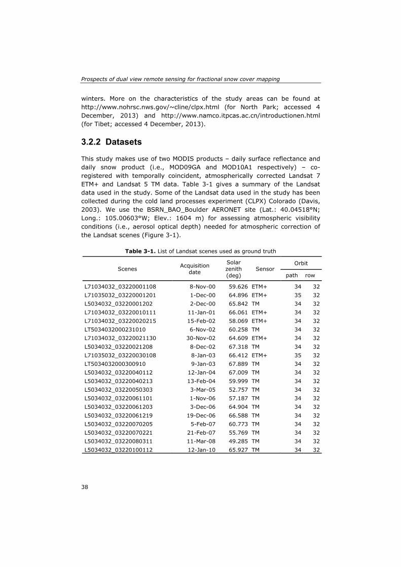
Prospects of dual view remote sensing for fractional snow cover mapping
winters. More on the characteristics of the study areas can be found at http://www.nohrsc.nws.gov/~cline/clpx.html (for North Park; accessed 4 December, 2013) and http://www.namco.itpcas.ac.cn/introductionen.html (for Tibet; accessed 4 December, 2013).
3.2.2 Datasets
This study makes use of two MODIS products – daily surface reflectance and daily snow product (i.e., MOD09GA and MOD10A1 respectively) – co-registered with temporally coincident, atmospherically corrected Landsat 7 ETM+ and Landsat 5 TM data. Table 3-1 gives a summary of the Landsat data used in the study. Some of the Landsat data used in the study has been collected during the cold land processes experiment (CLPX) Colorado (Davis, 2003). We use the BSRN_BAO_Boulder AERONET site (Lat.: 40.04518°N; Long.: 105.00603°W; Elev.: 1604 m) for assessing atmospheric visibility conditions (i.e., aerosol optical depth) needed for atmospheric correction of the Landsat scenes (Figure 3-1).
Table 3-1. List of Landsat scenes used as ground truth
Scenes Acquisition date
Solar zenith (deg)
Sensor Orbit
path row
L71034032_03220001108 8-Nov-00 59.626 ETM+ 34 32 L71035032_03220001201 1-Dec-00 64.896 ETM+ 35 32 L5034032_03220001202 2-Dec-00 65.842 TM 34 32 L71034032_03220010111 11-Jan-01 66.061 ETM+ 34 32 L71034032_03220020215 15-Feb-02 58.069 ETM+ 34 32 LT5034032000231010 6-Nov-02 60.258 TM 34 32 L71034032_03220021130 30-Nov-02 64.609 ETM+ 34 32 L5034032_03220021208 8-Dec-02 67.318 TM 34 32 L71035032_03220030108 8-Jan-03 66.412 ETM+ 35 32 LT5034032000300910 9-Jan-03 67.889 TM 34 32 L5034032_03220040112 12-Jan-04 67.009 TM 34 32 L5034032_03220040213 13-Feb-04 59.999 TM 34 32 L5034032_03220050303 3-Mar-05 52.757 TM 34 32 L5034032_03220061101 1-Nov-06 57.187 TM 34 32 L5034032_03220061203 3-Dec-06 64.904 TM 34 32 L5034032_03220061219 19-Dec-06 66.588 TM 34 32 L5034032_03220070205 5-Feb-07 60.773 TM 34 32 L5034032_03220070221 21-Feb-07 55.769 TM 34 32 L5034032_03220080311 11-Mar-08 49.285 TM 34 32 L5034032_03220100112 12-Jan-10 65.927 TM 34 32
38
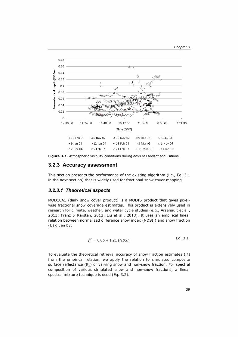
Chapter 3
Figure 3-1. Atmospheric visibility conditions during days of Landsat acquisitions
3.2.3 Accuracy assessment
This section presents the performance of the existing algorithm (i.e., Eq. 3.1 in the next section) that is widely used for fractional snow cover mapping.
3.2.3.1 Theoretical aspects
MOD10A1 (daily snow cover product) is a MODIS product that gives pixel-wise fractional snow coverage estimates. This product is extensively used in research for climate, weather, and water cycle studies (e.g., Arsenault et al., 2013; Franz & Karsten, 2013; Liu et al., 2013). It uses an empirical linear relation between normalized difference snow index (NDSI,) and snow fraction (fs) given by,
𝑓𝑠𝑟 = 0.06 + 1.21 (𝑁𝐷𝑆𝐼) Eq. 3.1
To evaluate the theoretical retrieval accuracy of snow fraction estimates (fsr) from the empirical relation, we apply the relation to simulated composite surface reflectance (Rλ) of varying snow and non-snow fraction. For spectral composition of various simulated snow and non-snow fractions, a linear spectral mixture technique is used (Eq. 3.2).
39
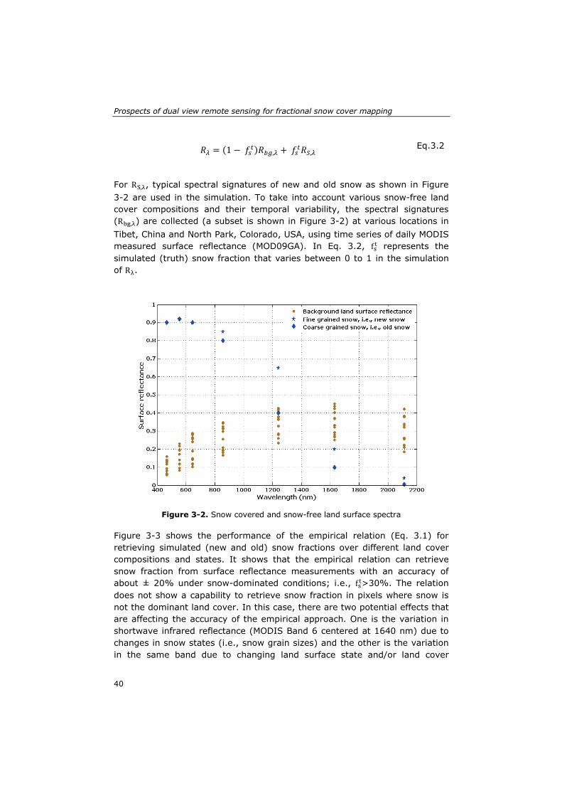
Prospects of dual view remote sensing for fractional snow cover mapping
𝑅𝜆 = (1 − 𝑓𝑠𝑡)𝑅𝑏𝑔,𝜆 + 𝑓𝑠𝑡𝑅𝑆,𝜆 Eq.3.2
For RS,λ, typical spectral signatures of new and old snow as shown in Figure 3-2 are used in the simulation. To take into account various snow-free land cover compositions and their temporal variability, the spectral signatures (Rbg,λ) are collected (a subset is shown in Figure 3-2) at various locations in Tibet, China and North Park, Colorado, USA, using time series of daily MODIS measured surface reflectance (MOD09GA). In Eq. 3.2, fst represents the simulated (truth) snow fraction that varies between 0 to 1 in the simulation of Rλ.
Figure 3-2. Snow covered and snow-free land surface spectra
Figure 3-3 shows the performance of the empirical relation (Eq. 3.1) for retrieving simulated (new and old) snow fractions over different land cover compositions and states. It shows that the empirical relation can retrieve snow fraction from surface reflectance measurements with an accuracy of about ± 20% under snow-dominated conditions; i.e., fst>30%. The relation does not show a capability to retrieve snow fraction in pixels where snow is not the dominant land cover. In this case, there are two potential effects that are affecting the accuracy of the empirical approach. One is the variation in shortwave infrared reflectance (MODIS Band 6 centered at 1640 nm) due to changes in snow states (i.e., snow grain sizes) and the other is the variation in the same band due to changing land surface state and/or land cover
40
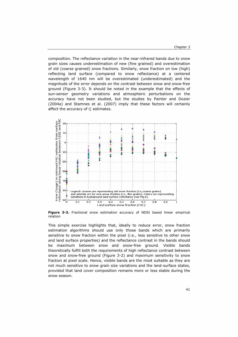
Chapter 3
composition. The reflectance variation in the near-infrared bands due to snow grain sizes causes underestimation of new (fine grained) and overestimation of old (coarse grained) snow fractions. Similarly, snow fraction on low (high) reflecting land surface (compared to snow reflectance) at a centered wavelength of 1640 nm will be overestimated (underestimated) and the magnitude of the error depends on the contrast between snow and snow-free ground (Figure 3-3). It should be noted in the example that the effects of sun-sensor geometry variations and atmospheric perturbations on the accuracy have not been studied, but the studies by Painter and Dozier (2004a) and Stamnes et al. (2007) imply that these factors will certainly affect the accuracy of fsr estimates.
Figure 3-3. Fractional snow estimation accuracy of NDSI based linear empirical relation
This simple exercise highlights that, ideally to reduce error, snow fraction estimation algorithms should use only those bands which are primarily sensitive to snow fraction within the pixel (i.e., less sensitive to other snow and land surface properties) and the reflectance contrast in the bands should be maximum between snow and snow-free ground. Visible bands theoretically fulfill both the requirements of high reflectance contrast between snow and snow-free ground (Figure 3-2) and maximum sensitivity to snow fraction at pixel scale. Hence, visible bands are the most suitable as they are not much sensitive to snow grain size variations and the land-surface states, provided that land cover composition remains more or less stable during the snow season.
41
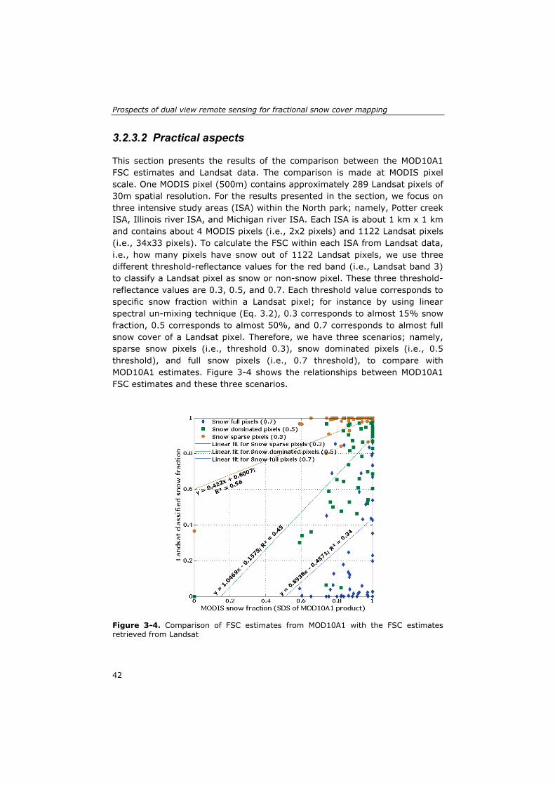
Prospects of dual view remote sensing for fractional snow cover mapping
3.2.3.2 Practical aspects
This section presents the results of the comparison between the MOD10A1 FSC estimates and Landsat data. The comparison is made at MODIS pixel scale. One MODIS pixel (500m) contains approximately 289 Landsat pixels of 30m spatial resolution. For the results presented in the section, we focus on three intensive study areas (ISA) within the North park; namely, Potter creek ISA, Illinois river ISA, and Michigan river ISA. Each ISA is about 1 km x 1 km and contains about 4 MODIS pixels (i.e., 2x2 pixels) and 1122 Landsat pixels (i.e., 34x33 pixels). To calculate the FSC within each ISA from Landsat data, i.e., how many pixels have snow out of 1122 Landsat pixels, we use three different threshold-reflectance values for the red band (i.e., Landsat band 3) to classify a Landsat pixel as snow or non-snow pixel. These three threshold-reflectance values are 0.3, 0.5, and 0.7. Each threshold value corresponds to specific snow fraction within a Landsat pixel; for instance by using linear spectral un-mixing technique (Eq. 3.2), 0.3 corresponds to almost 15% snow fraction, 0.5 corresponds to almost 50%, and 0.7 corresponds to almost full snow cover of a Landsat pixel. Therefore, we have three scenarios; namely, sparse snow pixels (i.e., threshold 0.3), snow dominated pixels (i.e., 0.5 threshold), and full snow pixels (i.e., 0.7 threshold), to compare with MOD10A1 estimates. Figure 3-4 shows the relationships between MOD10A1 FSC estimates and these three scenarios.
Figure 3-4. Comparison of FSC estimates from MOD10A1 with the FSC estimates retrieved from Landsat
42
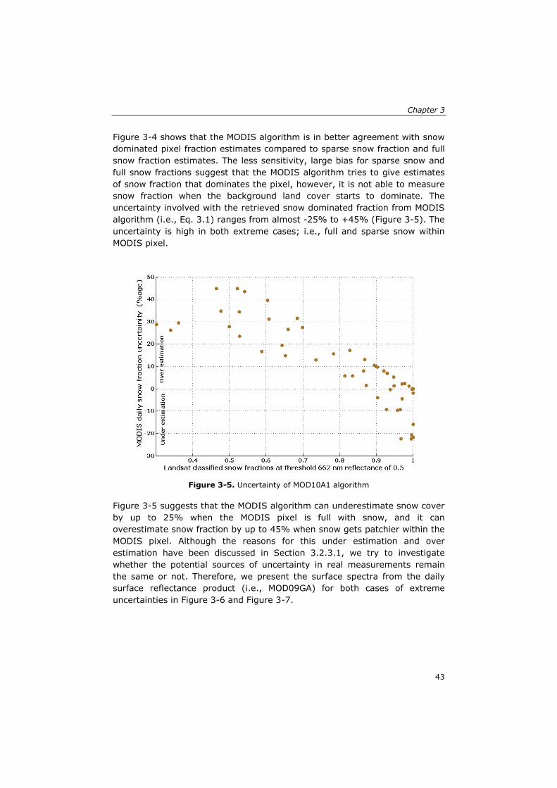
Chapter 3
Figure 3-4 shows that the MODIS algorithm is in better agreement with snow dominated pixel fraction estimates compared to sparse snow fraction and full snow fraction estimates. The less sensitivity, large bias for sparse snow and full snow fractions suggest that the MODIS algorithm tries to give estimates of snow fraction that dominates the pixel, however, it is not able to measure snow fraction when the background land cover starts to dominate. The uncertainty involved with the retrieved snow dominated fraction from MODIS algorithm (i.e., Eq. 3.1) ranges from almost -25% to +45% (Figure 3-5). The uncertainty is high in both extreme cases; i.e., full and sparse snow within MODIS pixel.
Figure 3-5. Uncertainty of MOD10A1 algorithm
Figure 3-5 suggests that the MODIS algorithm can underestimate snow cover by up to 25% when the MODIS pixel is full with snow, and it can overestimate snow fraction by up to 45% when snow gets patchier within the MODIS pixel. Although the reasons for this under estimation and over estimation have been discussed in Section 3.2.3.1, we try to investigate whether the potential sources of uncertainty in real measurements remain the same or not. Therefore, we present the surface spectra from the daily surface reflectance product (i.e., MOD09GA) for both cases of extreme uncertainties in Figure 3-6 and Figure 3-7.
43
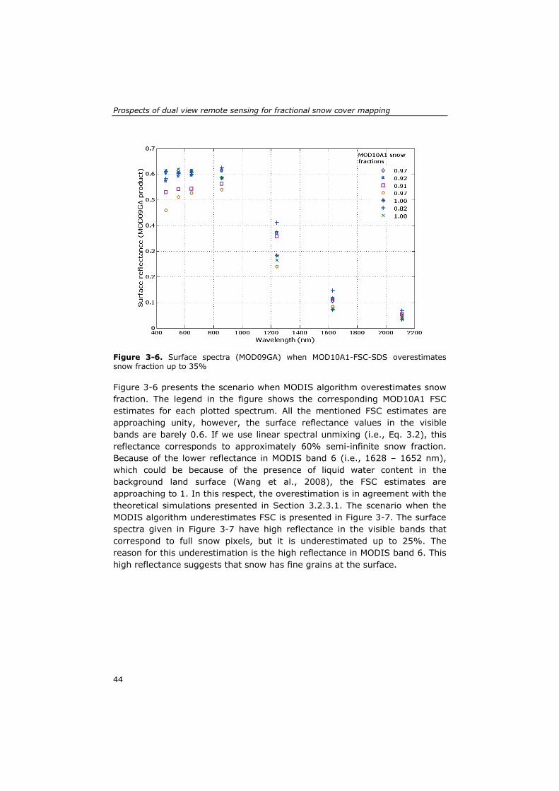
Prospects of dual view remote sensing for fractional snow cover mapping
Figure 3-6. Surface spectra (MOD09GA) when MOD10A1-FSC-SDS overestimates snow fraction up to 35%
Figure 3-6 presents the scenario when MODIS algorithm overestimates snow fraction. The legend in the figure shows the corresponding MOD10A1 FSC estimates for each plotted spectrum. All the mentioned FSC estimates are approaching unity, however, the surface reflectance values in the visible bands are barely 0.6. If we use linear spectral unmixing (i.e., Eq. 3.2), this reflectance corresponds to approximately 60% semi-infinite snow fraction. Because of the lower reflectance in MODIS band 6 (i.e., 1628 – 1652 nm), which could be because of the presence of liquid water content in the background land surface (Wang et al., 2008), the FSC estimates are approaching to 1. In this respect, the overestimation is in agreement with the theoretical simulations presented in Section 3.2.3.1. The scenario when the MODIS algorithm underestimates FSC is presented in Figure 3-7. The surface spectra given in Figure 3-7 have high reflectance in the visible bands that correspond to full snow pixels, but it is underestimated up to 25%. The reason for this underestimation is the high reflectance in MODIS band 6. This high reflectance suggests that snow has fine grains at the surface.
44
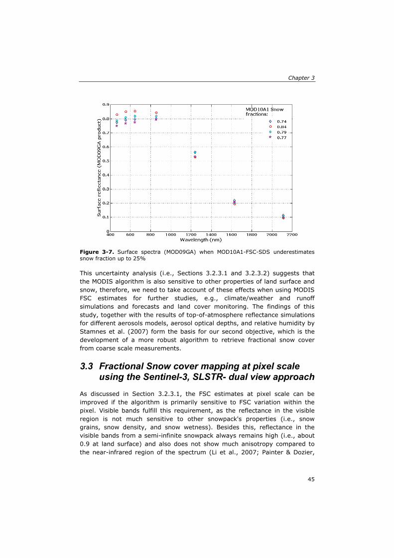
Chapter 3
Figure 3-7. Surface spectra (MOD09GA) when MOD10A1-FSC-SDS underestimates snow fraction up to 25%
This uncertainty analysis (i.e., Sections 3.2.3.1 and 3.2.3.2) suggests that the MODIS algorithm is also sensitive to other properties of land surface and snow, therefore, we need to take account of these effects when using MODIS FSC estimates for further studies, e.g., climate/weather and runoff simulations and forecasts and land cover monitoring. The findings of this study, together with the results of top-of-atmosphere reflectance simulations for different aerosols models, aerosol optical depths, and relative humidity by Stamnes et al. (2007) form the basis for our second objective, which is the development of a more robust algorithm to retrieve fractional snow cover from coarse scale measurements.
3.3 Fractional Snow cover mapping at pixel scale using the Sentinel-3, SLSTR- dual view approach
As discussed in Section 3.2.3.1, the FSC estimates at pixel scale can be improved if the algorithm is primarily sensitive to FSC variation within the pixel. Visible bands fulfill this requirement, as the reflectance in the visible region is not much sensitive to other snowpack's properties (i.e., snow grains, snow density, and snow wetness). Besides this, reflectance in the visible bands from a semi-infinite snowpack always remains high (i.e., about 0.9 at land surface) and also does not show much anisotropy compared to the near-infrared region of the spectrum (Li et al., 2007; Painter & Dozier,
45
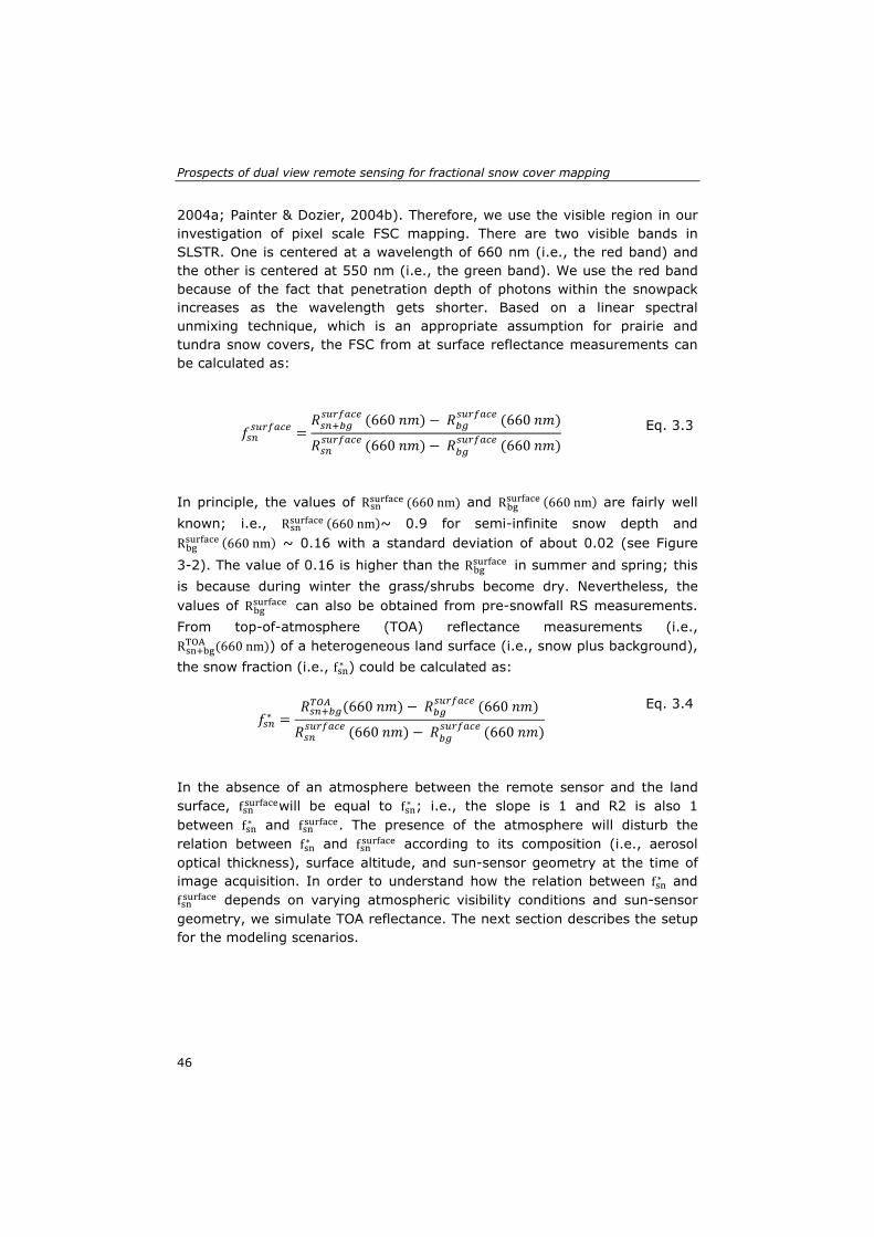
Prospects of dual view remote sensing for fractional snow cover mapping
2004a; Painter & Dozier, 2004b). Therefore, we use the visible region in our investigation of pixel scale FSC mapping. There are two visible bands in SLSTR. One is centered at a wavelength of 660 nm (i.e., the red band) and the other is centered at 550 nm (i.e., the green band). We use the red band because of the fact that penetration depth of photons within the snowpack increases as the wavelength gets shorter. Based on a linear spectral unmixing technique, which is an appropriate assumption for prairie and tundra snow covers, the FSC from at surface reflectance measurements can be calculated as:
𝑓𝑠𝑛𝑠𝑢𝑟𝑓𝑎𝑐𝑒 =
𝑅𝑠𝑛+𝑏𝑔𝑠𝑢𝑟𝑓𝑎𝑐𝑒 (660 𝑛𝑚) − 𝑅𝑏𝑔
𝑠𝑢𝑟𝑓𝑎𝑐𝑒 (660 𝑛𝑚)
𝑅𝑠𝑛𝑠𝑢𝑟𝑓𝑎𝑐𝑒 (660 𝑛𝑚) − 𝑅𝑏𝑔
𝑠𝑢𝑟𝑓𝑎𝑐𝑒 (660 𝑛𝑚) Eq. 3.3
In principle, the values of Rsnsurface (660 nm) and Rbg
surface (660 nm) are fairly well known; i.e., Rsn
surface (660 nm)~ 0.9 for semi-infinite snow depth and Rbgsurface (660 nm) ~ 0.16 with a standard deviation of about 0.02 (see Figure
3-2). The value of 0.16 is higher than the Rbgsurface in summer and spring; this
is because during winter the grass/shrubs become dry. Nevertheless, the values of Rbg
surface can also be obtained from pre-snowfall RS measurements. From top-of-atmosphere (TOA) reflectance measurements (i.e., Rsn+bgTOA (660 nm)) of a heterogeneous land surface (i.e., snow plus background),
the snow fraction (i.e., fsn∗ ) could be calculated as:
𝑓𝑠𝑛∗ =𝑅𝑠𝑛+𝑏𝑔𝑇𝑂𝐴 (660 𝑛𝑚) − 𝑅𝑏𝑔
𝑠𝑢𝑟𝑓𝑎𝑐𝑒 (660 𝑛𝑚)
𝑅𝑠𝑛𝑠𝑢𝑟𝑓𝑎𝑐𝑒 (660 𝑛𝑚) − 𝑅𝑏𝑔
𝑠𝑢𝑟𝑓𝑎𝑐𝑒 (660 𝑛𝑚)
Eq. 3.4
In the absence of an atmosphere between the remote sensor and the land surface, fsnsurfacewill be equal to fsn∗ ; i.e., the slope is 1 and R2 is also 1 between fsn∗ and fsnsurface. The presence of the atmosphere will disturb the relation between fsn∗ and fsnsurface according to its composition (i.e., aerosol optical thickness), surface altitude, and sun-sensor geometry at the time of image acquisition. In order to understand how the relation between fsn∗ and fsnsurface depends on varying atmospheric visibility conditions and sun-sensor geometry, we simulate TOA reflectance. The next section describes the setup for the modeling scenarios.
46
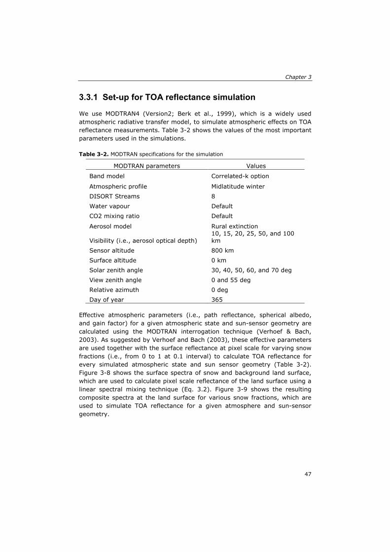
Chapter 3
3.3.1 Set-up for TOA reflectance simulation
We use MODTRAN4 (Version2; Berk et al., 1999), which is a widely used atmospheric radiative transfer model, to simulate atmospheric effects on TOA reflectance measurements. Table 3-2 shows the values of the most important parameters used in the simulations.
Table 3-2. MODTRAN specifications for the simulation
MODTRAN parameters Values
Band model Correlated-k option
Atmospheric profile Midlatitude winter DISORT Streams 8 Water vapour Default CO2 mixing ratio Default
Aerosol model Rural extinction
Visibility (i.e., aerosol optical depth) 10, 15, 20, 25, 50, and 100 km
Sensor altitude 800 km Surface altitude 0 km Solar zenith angle 30, 40, 50, 60, and 70 deg View zenith angle 0 and 55 deg Relative azimuth 0 deg Day of year 365
Effective atmospheric parameters (i.e., path reflectance, spherical albedo, and gain factor) for a given atmospheric state and sun-sensor geometry are calculated using the MODTRAN interrogation technique (Verhoef & Bach, 2003). As suggested by Verhoef and Bach (2003), these effective parameters are used together with the surface reflectance at pixel scale for varying snow fractions (i.e., from 0 to 1 at 0.1 interval) to calculate TOA reflectance for every simulated atmospheric state and sun sensor geometry (Table 3-2). Figure 3-8 shows the surface spectra of snow and background land surface, which are used to calculate pixel scale reflectance of the land surface using a linear spectral mixing technique (Eq. 3.2). Figure 3-9 shows the resulting composite spectra at the land surface for various snow fractions, which are used to simulate TOA reflectance for a given atmosphere and sun-sensor geometry.
47
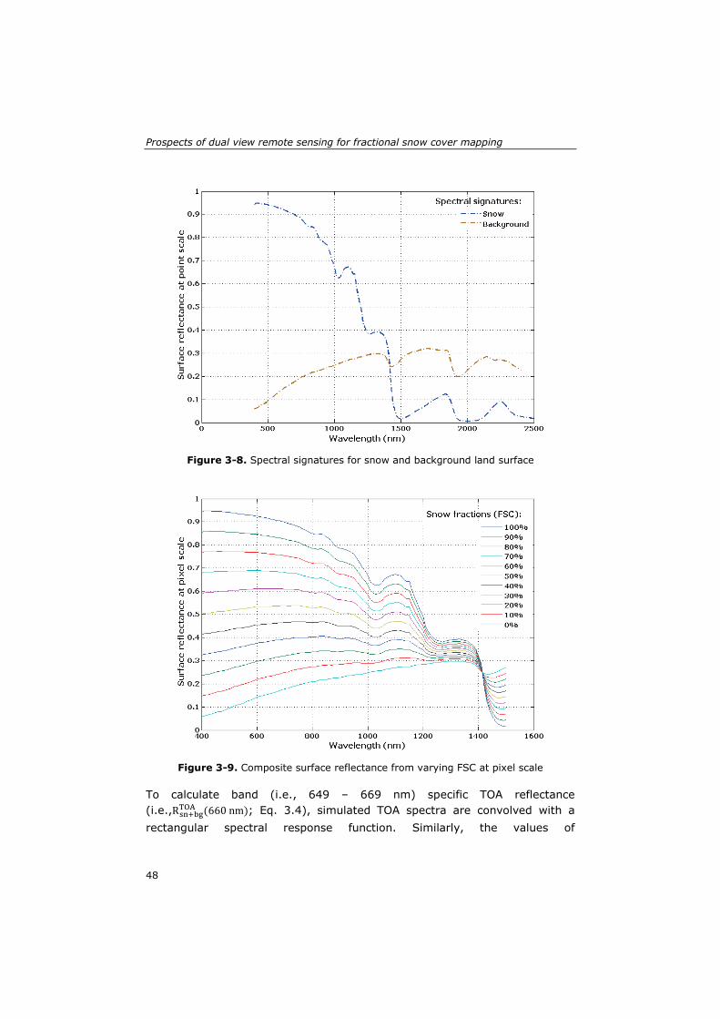
Prospects of dual view remote sensing for fractional snow cover mapping
Figure 3-8. Spectral signatures for snow and background land surface
Figure 3-9. Composite surface reflectance from varying FSC at pixel scale
To calculate band (i.e., 649 – 669 nm) specific TOA reflectance (i.e.,Rsn+bg
TOA (660 nm); Eq. 3.4), simulated TOA spectra are convolved with a rectangular spectral response function. Similarly, the values of
48
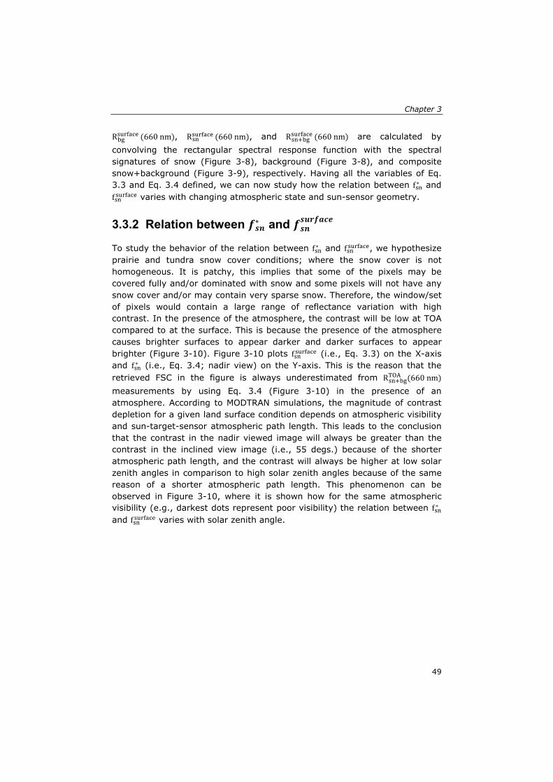
Chapter 3
Rbgsurface (660 nm), Rsn
surface (660 nm), and Rsn+bgsurface (660 nm) are calculated by
convolving the rectangular spectral response function with the spectral signatures of snow (Figure 3-8), background (Figure 3-8), and composite snow+background (Figure 3-9), respectively. Having all the variables of Eq. 3.3 and Eq. 3.4 defined, we can now study how the relation between fsn∗ and fsnsurface varies with changing atmospheric state and sun-sensor geometry.
3.3.2 Relation between 𝒇𝒔𝒏∗ and 𝒇𝒔𝒏𝒔𝒖𝒓𝒇𝒂𝒄𝒆
To study the behavior of the relation between fsn∗ and fsnsurface, we hypothesize prairie and tundra snow cover conditions; where the snow cover is not homogeneous. It is patchy, this implies that some of the pixels may be covered fully and/or dominated with snow and some pixels will not have any snow cover and/or may contain very sparse snow. Therefore, the window/set of pixels would contain a large range of reflectance variation with high contrast. In the presence of the atmosphere, the contrast will be low at TOA compared to at the surface. This is because the presence of the atmosphere causes brighter surfaces to appear darker and darker surfaces to appear brighter (Figure 3-10). Figure 3-10 plots fsnsurface (i.e., Eq. 3.3) on the X-axis and fsn∗ (i.e., Eq. 3.4; nadir view) on the Y-axis. This is the reason that the retrieved FSC in the figure is always underestimated from Rsn+bg
TOA (660 nm) measurements by using Eq. 3.4 (Figure 3-10) in the presence of an atmosphere. According to MODTRAN simulations, the magnitude of contrast depletion for a given land surface condition depends on atmospheric visibility and sun-target-sensor atmospheric path length. This leads to the conclusion that the contrast in the nadir viewed image will always be greater than the contrast in the inclined view image (i.e., 55 degs.) because of the shorter atmospheric path length, and the contrast will always be higher at low solar zenith angles in comparison to high solar zenith angles because of the same reason of a shorter atmospheric path length. This phenomenon can be observed in Figure 3-10, where it is shown how for the same atmospheric visibility (e.g., darkest dots represent poor visibility) the relation between fsn∗ and fsnsurface varies with solar zenith angle.
49
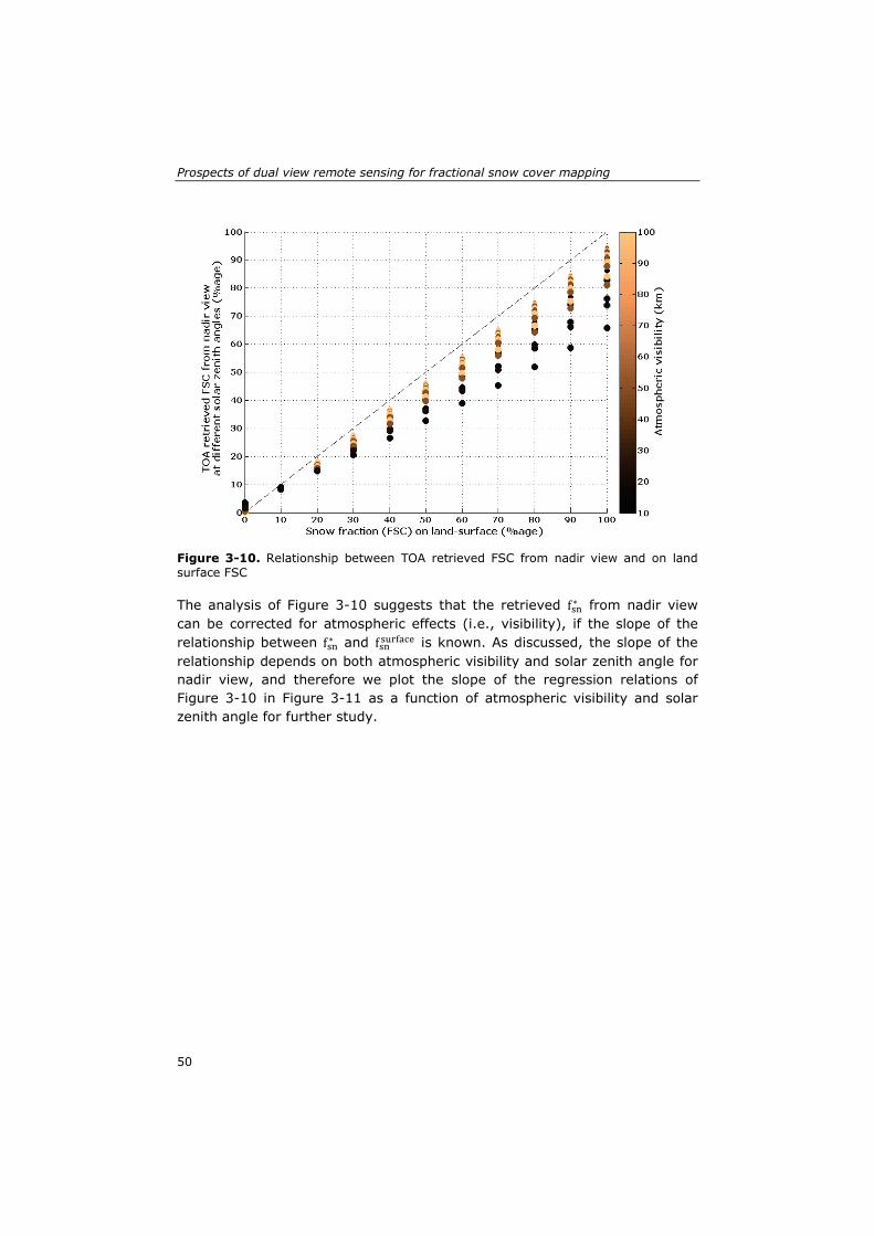
Prospects of dual view remote sensing for fractional snow cover mapping
Figure 3-10. Relationship between TOA retrieved FSC from nadir view and on land surface FSC
The analysis of Figure 3-10 suggests that the retrieved fsn∗ from nadir view can be corrected for atmospheric effects (i.e., visibility), if the slope of the relationship between fsn∗ and fsnsurface is known. As discussed, the slope of the relationship depends on both atmospheric visibility and solar zenith angle for nadir view, and therefore we plot the slope of the regression relations of Figure 3-10 in Figure 3-11 as a function of atmospheric visibility and solar zenith angle for further study.
50
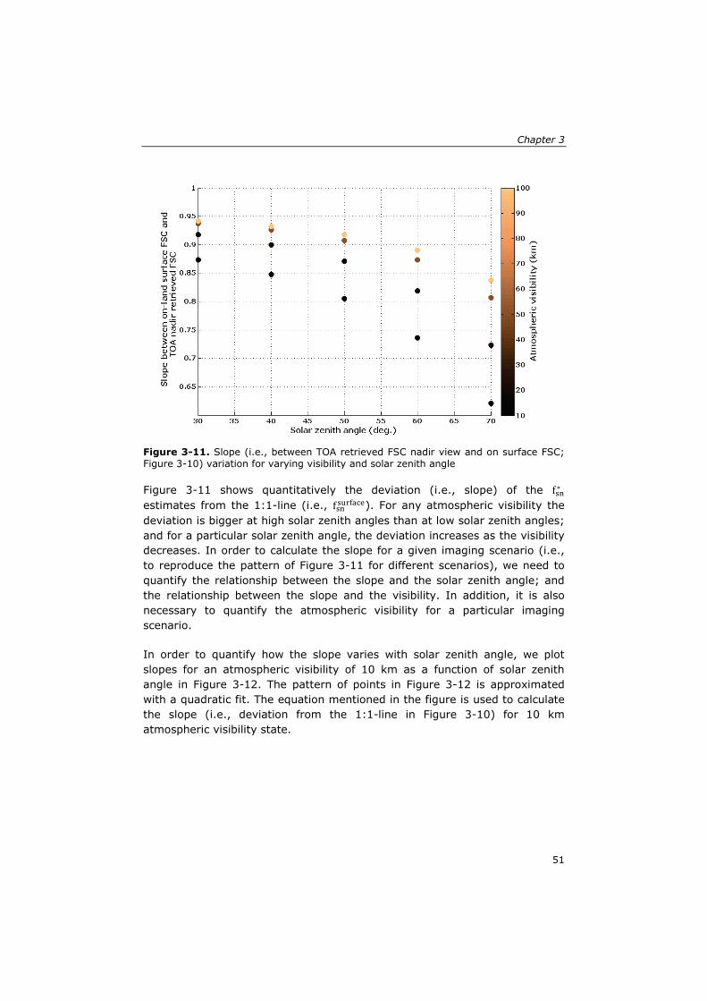
Chapter 3
Figure 3-11. Slope (i.e., between TOA retrieved FSC nadir view and on surface FSC; Figure 3-10) variation for varying visibility and solar zenith angle
Figure 3-11 shows quantitatively the deviation (i.e., slope) of the fsn∗ estimates from the 1:1-line (i.e., fsnsurface). For any atmospheric visibility the deviation is bigger at high solar zenith angles than at low solar zenith angles; and for a particular solar zenith angle, the deviation increases as the visibility decreases. In order to calculate the slope for a given imaging scenario (i.e., to reproduce the pattern of Figure 3-11 for different scenarios), we need to quantify the relationship between the slope and the solar zenith angle; and the relationship between the slope and the visibility. In addition, it is also necessary to quantify the atmospheric visibility for a particular imaging scenario.
In order to quantify how the slope varies with solar zenith angle, we plot slopes for an atmospheric visibility of 10 km as a function of solar zenith angle in Figure 3-12. The pattern of points in Figure 3-12 is approximated with a quadratic fit. The equation mentioned in the figure is used to calculate the slope (i.e., deviation from the 1:1-line in Figure 3-10) for 10 km atmospheric visibility state.
51
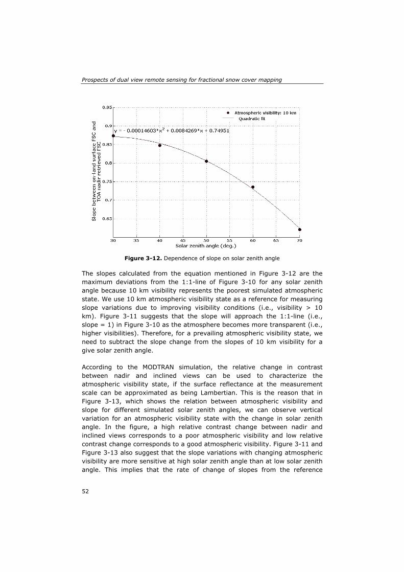
Prospects of dual view remote sensing for fractional snow cover mapping
Figure 3-12. Dependence of slope on solar zenith angle
The slopes calculated from the equation mentioned in Figure 3-12 are the maximum deviations from the 1:1-line of Figure 3-10 for any solar zenith angle because 10 km visibility represents the poorest simulated atmospheric state. We use 10 km atmospheric visibility state as a reference for measuring slope variations due to improving visibility conditions (i.e., visibility > 10 km). Figure 3-11 suggests that the slope will approach the 1:1-line (i.e., slope = 1) in Figure 3-10 as the atmosphere becomes more transparent (i.e., higher visibilities). Therefore, for a prevailing atmospheric visibility state, we need to subtract the slope change from the slopes of 10 km visibility for a give solar zenith angle.
According to the MODTRAN simulation, the relative change in contrast between nadir and inclined views can be used to characterize the atmospheric visibility state, if the surface reflectance at the measurement scale can be approximated as being Lambertian. This is the reason that in Figure 3-13, which shows the relation between atmospheric visibility and slope for different simulated solar zenith angles, we can observe vertical variation for an atmospheric visibility state with the change in solar zenith angle. In the figure, a high relative contrast change between nadir and inclined views corresponds to a poor atmospheric visibility and low relative contrast change corresponds to a good atmospheric visibility. Figure 3-11 and Figure 3-13 also suggest that the slope variations with changing atmospheric visibility are more sensitive at high solar zenith angle than at low solar zenith angle. This implies that the rate of change of slopes from the reference
52
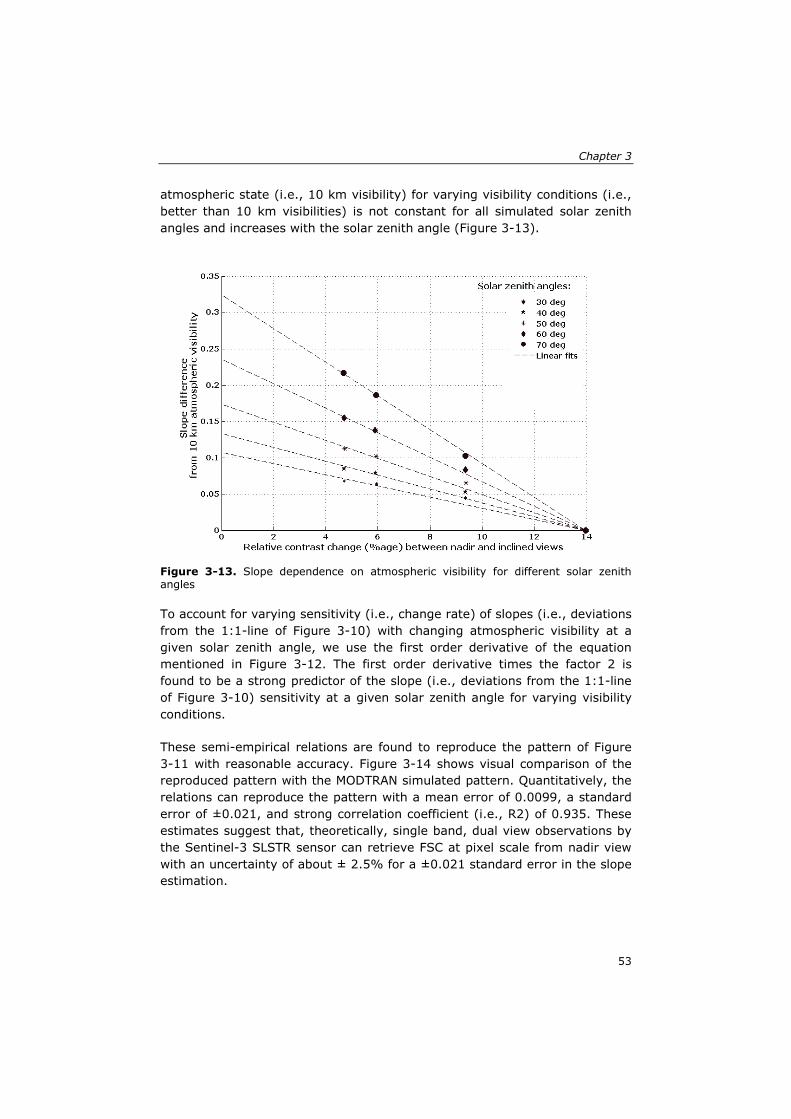
Chapter 3
atmospheric state (i.e., 10 km visibility) for varying visibility conditions (i.e., better than 10 km visibilities) is not constant for all simulated solar zenith angles and increases with the solar zenith angle (Figure 3-13).
Figure 3-13. Slope dependence on atmospheric visibility for different solar zenith angles
To account for varying sensitivity (i.e., change rate) of slopes (i.e., deviations from the 1:1-line of Figure 3-10) with changing atmospheric visibility at a given solar zenith angle, we use the first order derivative of the equation mentioned in Figure 3-12. The first order derivative times the factor 2 is found to be a strong predictor of the slope (i.e., deviations from the 1:1-line of Figure 3-10) sensitivity at a given solar zenith angle for varying visibility conditions.
These semi-empirical relations are found to reproduce the pattern of Figure 3-11 with reasonable accuracy. Figure 3-14 shows visual comparison of the reproduced pattern with the MODTRAN simulated pattern. Quantitatively, the relations can reproduce the pattern with a mean error of 0.0099, a standard error of ±0.021, and strong correlation coefficient (i.e., R2) of 0.935. These estimates suggest that, theoretically, single band, dual view observations by the Sentinel-3 SLSTR sensor can retrieve FSC at pixel scale from nadir view with an uncertainty of about ± 2.5% for a ±0.021 standard error in the slope estimation.
53
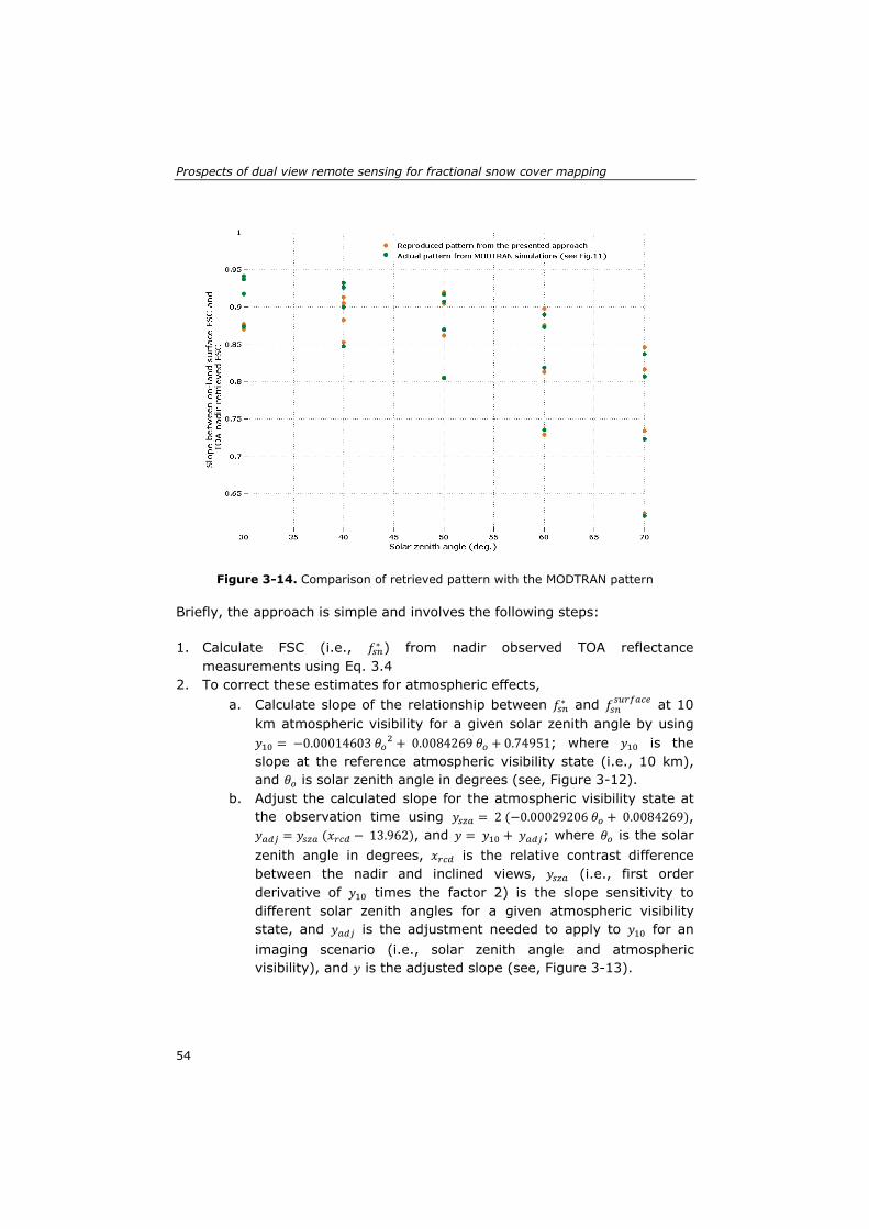
Prospects of dual view remote sensing for fractional snow cover mapping
Figure 3-14. Comparison of retrieved pattern with the MODTRAN pattern
Briefly, the approach is simple and involves the following steps:
1. Calculate FSC (i.e., 𝑓𝑠𝑛∗ ) from nadir observed TOA reflectance measurements using Eq. 3.4
2. To correct these estimates for atmospheric effects, a. Calculate slope of the relationship between 𝑓𝑠𝑛∗ and 𝑓𝑠𝑛
𝑠𝑢𝑟𝑓𝑎𝑐𝑒 at 10 km atmospheric visibility for a given solar zenith angle by using 𝑦10 = −0.00014603 𝜃𝑜2 + 0.0084269 𝜃𝑜 + 0.74951; where 𝑦10 is the slope at the reference atmospheric visibility state (i.e., 10 km), and 𝜃𝑜 is solar zenith angle in degrees (see, Figure 3-12).
b. Adjust the calculated slope for the atmospheric visibility state at the observation time using 𝑦𝑠𝑧𝑎 = 2 (−0.00029206 𝜃𝑜 + 0.0084269), 𝑦𝑎𝑑𝑗 = 𝑦𝑠𝑧𝑎 (𝑥𝑟𝑐𝑑 − 13.962), and 𝑦 = 𝑦10 + 𝑦𝑎𝑑𝑗; where 𝜃𝑜 is the solar zenith angle in degrees, 𝑥𝑟𝑐𝑑 is the relative contrast difference between the nadir and inclined views, 𝑦𝑠𝑧𝑎 (i.e., first order derivative of 𝑦10 times the factor 2) is the slope sensitivity to different solar zenith angles for a given atmospheric visibility state, and 𝑦𝑎𝑑𝑗 is the adjustment needed to apply to 𝑦10 for an imaging scenario (i.e., solar zenith angle and atmospheric visibility), and 𝑦 is the adjusted slope (see, Figure 3-13).
54
Chapter 3
3. Apply corrections to 𝑓𝑠𝑛∗ to get 𝑓𝑠𝑛𝑠𝑢𝑟𝑓𝑎𝑐𝑒 by using 𝑓𝑠𝑛
𝑠𝑢𝑟𝑓𝑎𝑐𝑒 = 𝑓𝑠𝑛∗
𝑦 (see, Figure
3-10)
Although the approach in terms of accuracy (i.e., uncertainty estimates) is more accurate than the approach used in MOD10A1 product (Section 3.2.3.1), it also has some limitations. This approach overestimates FSC within pixels that have very little or no snow on the land surface, because we have assumed zero offset in Figure 3-10. Besides this, we have also assumed Lambertian reflection for the snow surface. Although a Lambertian reflectance assumption for snow may be reasonable at coarse scale reflectance measurements in the visible bands (Lyapustin et al., 2009), this may induce some inaccuracy (i.e., uncertainty) in the retrieved estimates (see Chapter 2). For the TOA reflectance simulation, we have used MODTRAN which is considered as state-of-the-art radiative transfer model. MODTRAN treats the atmosphere as homogeneous layers. Therefore, lateral homogeneity of the atmosphere is also assumed between the nadir and inclined views in the presented study. There are other issues that also need to be addressed in future; for instance regarding the evolution of the pattern (i.e., Figure 3-11) for different surface altitudes and relative azimuth angles between the sun and sensor.
3.4 Discussion and conclusions This chapter addresses two objectives regarding fractional snow coverage (FSC) mapping at pixel scale from moderate resolution remote sensors. Our first objective is the quantification of the uncertainty in MOD10A1 product of MODIS. The other objective is assessment of potentials for FSC mapping from Sea Land Surface Temperature Radiometer (SLSTR) of Sentinel-3 mission. MOD10A1 is a daily snow product, which uses a linear empirical relation between NDSI and FSC to map fractional snow cover within a pixel. This study shows that the algorithm attempts to calculate the snow-dominated fraction (i.e., that contains at least 45 to 50% semi-infinite snowpack fraction at TM/ETM measurement scale) within a MODIS pixel. Although the retrieved fractions are not very accurate (R2 = 0.45), the estimates become more uncertain in the extreme conditions of fully-covered snow (semi-infinite) and sparse snow pixels. The comparison of MODIS daily snow fractions with Landsat images reveals that the algorithm underestimates snow fraction by up to 25% when the pixel is full with snow and overestimates snow fraction by up to 35% in sparse snow pixels. Since the algorithm uses top-of-atmosphere reflectance for retrieving the snow fraction, the perturbation in the visible reflectance measurements due to atmospheric variation is one source of uncertainty in the estimates. The other source of uncertainty, that this study highlights, is the reflectance variation in
55
Prospects of dual view remote sensing for fractional snow cover mapping
the infrared bands of the solar spectrum due to changing sun-sensor geometry, snow grain size and background land surface state (if snow cover is patchy in the pixel). This source of error in the estimates requires careful usage to characterize the observed land surface state (i.e., land-cover composition) for hydro and/or climate model state initialization as well as for multi-temporal analysis of land-cover variation. From data assimilation perspective in climate and hydrological models, the estimates are not the best candidate for a direct-insertion technique; but with the given accuracy assessment the estimates can be assimilated by using other stochastic techniques; like, ensemble Kalman filter (EnKF), or particle filter, to improve energy and water fluxes simulations.
Regarding the potentials of SLSTR for FSC mapping, this study shows very promising results that would allow more accurate FSC estimates from this sensor. Therefore, these estimates could be used with more confidence in climate and hydrological models. Dual view capability of the sensor provides a very effective way to account for the atmospheric effects on the retrieved estimates. In comparison to MOD10A1 retrieval approach, the presented approach using SLSTR is more robust, because it uses the visible region for FSC mapping, which is the most sensitive region for FSC variation within a pixel. However, there are some concerns that need to be addressed in the future for the development of a real operational algorithm for FSC mapping from SLSTR observations; especially, the effects of surface altitude variations and relative azimuth angle variation between the sun and sensor need some attention.
56
4 Improving modeled snow albedo estimates during the spring melt season
Abstract
Snow albedo influences snow-covered land energy and water budgets and is thus an important variable for energy and water fluxes calculations. Here, we quantify the performance of the three existing snow albedo parameterizations under alpine, tundra, and prairie snow conditions when implemented in the Noah land surface model (LSM) – Noah’s default and ones from the Biosphere-Atmosphere Transfer Scheme (BATS) and the Canadian Land Surface Scheme (CLASS) LSMs. The Noah LSM is forced with and its output is evaluated using in situ measurements from seven sites in U.S. and France. Comparison of the snow albedo simulations with the in situ measurements reveals that the three parameterizations overestimate snow albedo during springtime. An alternative snow albedo parameterization is introduced that adopts the shape of the variogram for the optically thick snowpacks and decreases the albedo further for optically thin conditions by mixing the snow with the land surface (background) albedo as a function of snow depth. In comparison with the in situ measurements, the new parameterization improves albedo simulation of the alpine and tundra snowpacks and positively impacts the simulation of snow depth, snowmelt rate, and upward shortwave radiation. An improved model performance with the variogram-shaped parameterization can, however, not be unambiguously detected for prairie snowpacks, which may be attributed to uncertainties associated with the simulation of snow density. An assessment of the model performance for the Upper Colorado River Basin highlights that with the variogram-shaped parameterization Noah simulates more evapotranspiration and larger runoff peaks in Spring, whereas the Summer runoff is lower.
Based on
Malik, M. J., R. van der Velde, Z. Vekerdy, and Z. Su (2014). Improving modeled snow albedo estimates during the spring melt season. Journal of Geophysical Research, doi: 10.1002/2013JD021344.
57
Improved modeling of snow albedo during melt-season
4.1 Introduction Snow cover dynamics are important for weather, climate, and hydrological studies via its control on the length of snow seasons, the timing and rate of snowmelt and streamflow, and the magnitude of energy and water fluxes at the land-atmosphere interface [Barnett et al., 2005; Souma and Wang, 2010]. Snow albedo and snow water equivalent (SWE) are the variables of a snowpack that affect land-surface’s energy and water budgets (Barlage et al., 2010; Malik et al., 2012). The SWE defines the liquid water volume within the snowpack, whereas the snow albedo determines directly the reflection of shortwave solar radiation at the snow-atmosphere interface and thus the total incoming net radiation. Indirectly, the snow albedo affects also the snow mass because the melting rate largely depends on the total incoming net radiation. As such, the snow albedo forms the direct link between energy and (snow) mass budgets. Amelioration of the snow albedo simulation within models will, therefore, improve simulation of surface energy budget as well as snow mass.
On global and continental scales, the energy fluxes at the land-atmosphere interface defined by the snow albedo impact also the stratosphere and troposphere and thus climate. Allen and Zender ( 2 0 1 0 ) , Fletcher et al. ( 2 0 0 9 a ) , Fletcher et al. ( 2 0 0 9 b ) , and Randall et al. ( 1 9 9 4 ) showed that t h e snow albedo feedback is the primary mechanism by which snow affects atmospheric circulation, especially during springtime, by altering the geopotential heights. Moreover, Lynch et al. ( 1 9 9 8 ) and Qu and Hall (2006) demonstrated that the climate simulated by a regional climate model is sensitive to the choice of t h e snow albedo parameterization in the land surface model (LSM). On the other hand, many studies ( e.g., Feng et al., 2008; Koivusalo & Heikinheimo, 1999; Molotch & Bales, 2006; Xue et al., 2003) have shown that improved snow albedo calculations contribute to the reliability of snow mass and melt simulations. Similarly, Malik et al. (2012) showed that improved snow albedo representation within the Noah LSM through assimilation of observations improves not only the simulation of snowpack properties but also the simulation of radiative fluxes. These findings highlight the importance of snow albedo for modeling various hydro-meteorological processes.
Snow albedo depends primarily on the grain size and is typically lower for snowpacks with larger grains (e.g., Malik et al., 2011, i.e., Chapter 2; Wiscombe & Warren, 1980). Over time, snow grains grow because of thawing and refreezing processes referred to as snow metamorphism. Spatially variable atmospheric forcings induce spatially variable metamorphism rates. Thus, the snow albedo varies over both space and time, which complicates snow albedo modeling. Within land surface (e.g., Noah, Biosphere-
58

Chapter 4
Atmosphere Transfer Scheme (BATS), Canadian Land Surface Scheme (CLASS), Variable Infiltration Capacity (VIC)) and hydrological (e.g., Distributed Hydrology Soil Vegetation Model) models, the snow albedo is commonly modeled as a function that decays with snow age. Although implementations of the snow albedo decay have improved hydro-meteorological simulations (Livneh et al., 2010), still uncertainties exist mainly due to the oversimplified handling of the complex snow albedo decay during the melt season where snowpacks disappear (Picard et al., 2012; Zender, 2012).
We explore an alternative snow albedo parameterization for LSMs through comparisons of offline simulations with observations for better characterization of the evolution of snow albedo during the melt season so as to improve the simulation of snow states and surface energy and water budgets as well. We investigate the snow albedo decay during springtime using in situ measurements collected under alpine, tundra, and prairie snowpack conditions and assess performance of four snow albedo parameterizations when implemented within the Noah LSM (Ek et al., 2003). In addition to Noah’s default option, a newly developed and two existing snow albedo parameterizations from BATS and CLASS are included in the analysis.
The in situ measurements used for this study have been collected throughout the globe under various conditions and include five alpine sites, one tundra site, and two prairie sites. Data from four of the alpine and one of the prairie sites are from the 2002-2003 Cold Land Processes Field Experiment (CLPX) campaign in Colorado, U.S. Another alpine snow data set is from a French site located in the Chartreuse mountain range of the Rhone-Alps. The tundra snow data set has been collected in Alaska, U.S. as a part of the AmeriFlux network, and the second prairie snow data set has been acquired from the Tibetan Plateau. The eight snow data sets all comprise measurements of both land-surface and near-surface atmospheric variables and form, as such, a comprehensive platform for providing new insights into snow albedo decay processes and evaluating the performance of the existing and new parameterizations.
This chapter is organized as follows. Sections 4.2 and 4.3 introduce the test sites and the in situ measurements, respectively. Section 4.4 describes the observed snow albedo evolution. Section 4.5 presents the relevant Noah LSM physics and snow albedo parameterizations. Section 4.6 presents assessment of the parameterizations and its impacts on snow depth and energy/mass flux simulations through a comparison of the Noah LSM simulations with the in situ measurements. Implications of the snow albedo parameterization at a
59
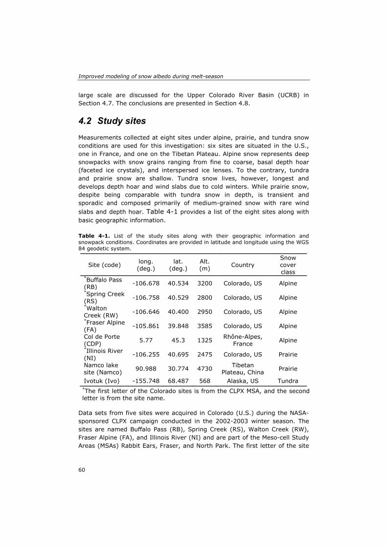
Improved modeling of snow albedo during melt-season
large scale are discussed for the Upper Colorado River Basin (UCRB) in Section 4.7. The conclusions are presented in Section 4.8.
4.2 Study sites Measurements collected at eight sites under alpine, prairie, and tundra snow conditions are used for this investigation: six sites are situated in the U.S., one in France, and one on the Tibetan Plateau. Alpine snow represents deep snowpacks with snow grains ranging from fine to coarse, basal depth hoar (faceted ice crystals), and interspersed ice lenses. To the contrary, tundra and prairie snow are shallow. Tundra snow lives, however, longest and develops depth hoar and wind slabs due to cold winters. While prairie snow, despite being comparable with tundra snow in depth, is transient and sporadic and composed primarily of medium-grained snow with rare wind slabs and depth hoar. Table 4-1 provides a list of the eight sites along with basic geographic information.
Table 4-1. List of the study sites along with their geographic information and snowpack conditions. Coordinates are provided in latitude and longitude using the WGS 84 geodetic system.
Site (code) long. (deg.)
lat. (deg.)
Alt. (m) Country
Snow cover class
*Buffalo Pass (RB) -106.678 40.534 3200 Colorado, US Alpine *Spring Creek (RS) -106.758 40.529 2800 Colorado, US Alpine *Walton Creek (RW) -106.646 40.400 2950 Colorado, US Alpine *Fraser Alpine (FA) -105.861 39.848 3585 Colorado, US Alpine
Col de Porte (CDP) 5.77 45.3 1325 Rhône-Alpes,
France Alpine *Illinois River (NI) -106.255 40.695 2475 Colorado, US Prairie
Namco lake site (Namco) 90.988 30.774 4730 Tibetan
Plateau, China Prairie
Ivotuk (Ivo) -155.748 68.487 568 Alaska, US Tundra *The first letter of the Colorado sites is from the CLPX MSA, and the second letter is from the site name.
Data sets from five sites were acquired in Colorado (U.S.) during the NASA-sponsored CLPX campaign conducted in the 2002-2003 winter season. The sites are named Buffalo Pass (RB), Spring Creek (RS), Walton Creek (RW), Fraser Alpine (FA), and Illinois River (NI) and are part of the Meso-cell Study Areas (MSAs) Rabbit Ears, Fraser, and North Park. The first letter of the site
60
Chapter 4
code in Table 4-1 refers to its corresponding MSA. The CLPX sites are located in a diverse landscape including broad glades, meadows, and grasslands. The NI site is situated in low rolling terrain, the sites RB, RS, and RW are located on mountain slopes, and the FA site resides on a mountain top. The differences in elevation create weather variability over small spatial and short temporal scales. The Fraser MSA is cooler than the two other MSAs mainly due to a higher elevation. Heavy snowfall often occurs at Rabbit Ears because of orographic effects, which results in the deepest alpine snowpacks at the site (e.g., Buffalo Pass) with the highest elevation of the MSA in Colorado. On the other hand, North Park experiences relatively little snowfall because it is situated in a mountain shadow area. Additionally, wind and sublimation contribute to the distribution of the shallow snowpacks at North Park as is typical for prairie snow conditions. More information on CLPX can be found at http://www.nohrsc.nws.gov/~cline/clpx.html (accessed 4 December 2013).
The other alpine site is the Col de Porte (CDP) site located in a grassy meadow at an altitude of 1325 m in the Chartreuse mountain range, France. Meteo-France operates this site in collaboration with other institutions since 1959. Continuous snow cover from late fall (December) to early spring (April) and low wind speeds characterize the area. Snow drift is thus limited in the area, and snowpacks may reach depths up to 1.5 m.
Ivotuk (Ivo) is the tundra site located on the north slope of the Brooks Range in Alaska, U.S. The land cover of the site is open shrubland with little relief. The site is part of Ameriflux network supported by the U.S. Global Change Research program, which focuses on the observations of energy, water, and carbon fluxes. In this region, snow accumulation starts at the end of September and reaches a total depth of about 65 cm before the onset of the melting period in May. Mid-winter melt events are quite rare. In the open terrain, weathering effects (e.g., cold wind) on the snowpack are strong, creating stratified snowpacks with depth hoar and relict wind crusts.
The data set of albedo measurements from the Tibetan Plateau is collected near the Namco Lake at an elevation of about 4700 m, used only for confirming the albedo evolution observed at the other shallow snowpack sites (i.e., Ivo and NI). The Institute for Tibetan Plateau Research of the Chinese Academy of Sciences (ITP-CAS) operates a permanent meteorological station equipped with a 20 m planetary boundary layer tower about 100 m from the shores of the lake. The land cover in the direct periphery is dominated by grassland with very little relief, but situated 10 km toward the south is a mountain range with peaks above 6000 m. The snowpacks are shallow, transient, and intermittent as is typical for prairie snow type conditions. The detailed description of this site can be found on website
61
Improved modeling of snow albedo during melt-season
http://www.namco.itpcas.ac.cn/introductionen.html (accessed 4 December 2013).
4.3 Data sets The data sets available for the sites, except for the Namco site, include measurements of atmospheric forcings and snow properties needed for running the Noah LSM and evaluating its simulations (Elder & Goodbody, 2004; Elder et al., 2009; Morin et al., 2012; Oechel, 2012). The near-surface atmospheric forcing data set comprises the measurements of air temperature, air humidity, surface pressure, wind speed, precipitation, and downward short- and longwave radiations. The atmospheric variables were measured approximately 1.5 m above the maximum anticipated snow depth at time intervals of 10, 30, and 60 min for the CLPX sites, Ivo, and CDP sites, respectively. Surface and soil temperatures as well as soil moisture measurements are used for the model initialization. The meteorological towers were also equipped with instrumentation for measuring snow depths surface albedo, and upward shortwave radiations. These measurements together with snowmelt measurements for the CDP site are used in this investigation for assessing the model performance.
Table 4-2 lists the instruments deployed at the sites along with their reported specifications.
62
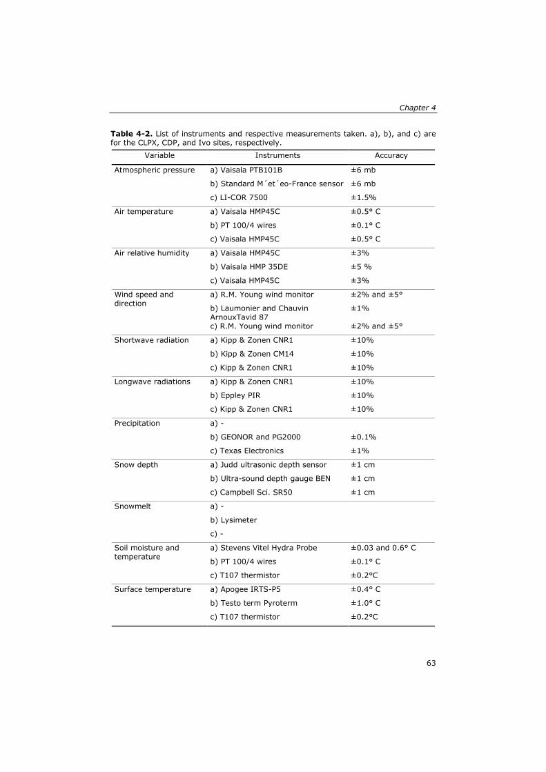
Chapter 4
Table 4-2. List of instruments and respective measurements taken. a), b), and c) are for the CLPX, CDP, and Ivo sites, respectively.
Variable Instruments Accuracy
Atmospheric pressure a) Vaisala PTB101B ±6 mb
b) Standard M´et´eo-France sensor ±6 mb
c) LI-COR 7500 ±1.5%
Air temperature a) Vaisala HMP45C ±0.5° C
b) PT 100/4 wires ±0.1° C
c) Vaisala HMP45C ±0.5° C
Air relative humidity a) Vaisala HMP45C ±3%
b) Vaisala HMP 35DE ±5 %
c) Vaisala HMP45C ±3%
Wind speed and direction
a) R.M. Young wind monitor ±2% and ±5°
b) Laumonier and Chauvin ArnouxTavid 87
±1%
c) R.M. Young wind monitor ±2% and ±5°
Shortwave radiation a) Kipp & Zonen CNR1 ±10%
b) Kipp & Zonen CM14 ±10%
c) Kipp & Zonen CNR1 ±10%
Longwave radiations a) Kipp & Zonen CNR1 ±10%
b) Eppley PIR ±10%
c) Kipp & Zonen CNR1 ±10%
Precipitation a) -
b) GEONOR and PG2000 ±0.1%
c) Texas Electronics ±1%
Snow depth a) Judd ultrasonic depth sensor ±1 cm
b) Ultra-sound depth gauge BEN ±1 cm
c) Campbell Sci. SR50 ±1 cm
Snowmelt a) -
b) Lysimeter
c) -
Soil moisture and temperature
a) Stevens Vitel Hydra Probe ±0.03 and 0.6° C
b) PT 100/4 wires ±0.1° C
c) T107 thermistor ±0.2°C
Surface temperature a) Apogee IRTS-P5 ±0.4° C
b) Testo term Pyroterm ±1.0° C
c) T107 thermistor ±0.2°C
63
Improved modeling of snow albedo during melt-season
Precipitation, needed to force the LSM, was not measured at the CLPX sites. Therefore, the precipitation inputs are obtained from the North American Land Data Assimilation System (NLDAS) for the sites. The NLDAS-2 precipitation product (Ek et al., 2011; Xia et al., 2012) is an hourly merged radar-gauge product at 1/8th degree (~ 12.5 km) spatial resolution, which is widely used for research purposes (e.g., Feng et al., 2008).
4.4 Measured snow albedo decay during melting period
Figure 4-1 shows the in situ measurements of snow albedo and snow depth made at four of the five alpine sites. Since the solar zenith angle affects snow albedo by altering penetration depth of solar insolation (Wiscombe & Warren, 1980), the values shown are the measurements taken around the local noontime +/- 2 h. The fairly small daily albedo variations suggest that the measurements were mostly collected under cloud free conditions. The figure highlights the important features of albedo evolution during melt season common for all the alpine sites from the onset of melting. The most prominent features are that the albedo i) drops to the minimum value of 0.45 - 0.5, ii) stays around this value as long as the snowpack remains optically thick (i.e., snow depth ≥ 50 cm for the springtime melting snowpack), and iii) starts to decrease again when snowpack becomes optically thin (i.e., snow depth < 50 cm for the springtime melting snowpack) because from that instant on the albedo is no longer a function of snow albedo alone and also depends on background albedo (viz. albedo of land-surface beneath the snowpack). Cline (1997b) has made similar observations regarding the albedo decay during the melting periods of the 1993-1994 and 1995-1996 snow seasons at the Niwot Long-Term Ecological Research site in the Colorado Front Range.
64
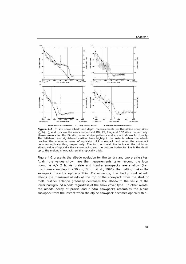
Chapter 4
Figure 4-1. In situ snow albedo and depth measurements for the alpine snow sites. a), b), c), and d) show the measurements at RB, RS, RW, and CDP sites, respectively. Measurements for the FA site reveal similar patterns and are not shown for brevity. The left-hand and right-hand vertical lines highlight the instants when the albedo reaches the minimum value of optically thick snowpack and when the snowpack becomes optically thin, respectively. The top horizontal line indicates the minimum albedo value of optically thick snowpacks, and the bottom horizontal line is the depth up to the melting snowpack remains optically thick.
Figure 4-2 presents the albedo evolution for the tundra and two prairie sites. Again, the values shown are the measurements taken around the local noontime +/- 2 h. As prairie and tundra snowpacks are shallow (i.e., maximum snow depth ~ 50 cm; Sturm et al., 1995), the melting makes the snowpack instantly optically thin. Consequently, the background albedo affects the measured albedo at the top of the snowpack from the start of melt. Further ablation gradually decreases the albedo to the value of the lower background albedo regardless of the snow cover type. In other words, the albedo decay of prairie and tundra snowpacks resembles the alpine snowpack from the instant when the alpine snowpack becomes optically thin.
65
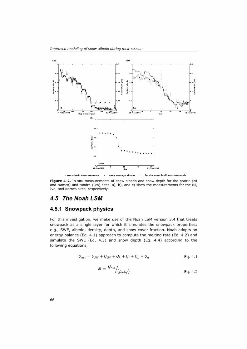
Improved modeling of snow albedo during melt-season
Figure 4-2. In situ measurements of snow albedo and snow depth for the prairie (NI and Namco) and tundra (Ivo) sites. a), b), and c) show the measurements for the NI, Ivo, and Namco sites, respectively.
4.5 The Noah LSM
4.5.1 Snowpack physics
For this investigation, we make use of the Noah LSM version 3.4 that treats snowpack as a single layer for which it simulates the snowpack properties: e.g., SWE, albedo, density, depth, and snow cover fraction. Noah adopts an energy balance (Eq. 4.1) approach to compute the melting rate (Eq. 4.2) and simulate the SWE (Eq. 4.3) and snow depth (Eq. 4.4) according to the following equations,
𝑄𝑛𝑒𝑡 = 𝑄𝑆𝑊 + 𝑄𝐿𝑊 + 𝑄ℎ + 𝑄𝑙 + 𝑄𝑔 + 𝑄𝑎 Eq. 4.1
𝑀 = 𝑄𝑛𝑒𝑡 �𝜌𝑤𝐿𝑓��
Eq. 4.2
66
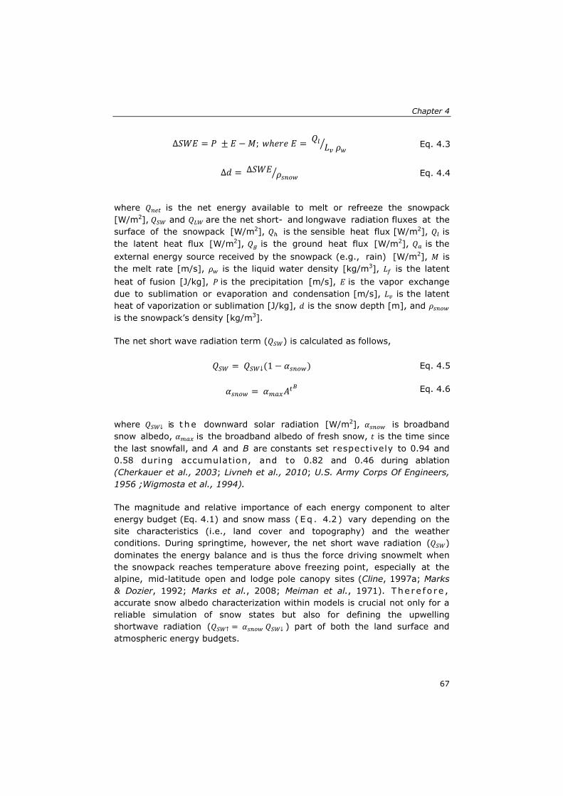
Chapter 4
∆𝑆𝑊𝐸 = 𝑃 ± 𝐸 −𝑀; 𝑤ℎ𝑒𝑟𝑒 𝐸 = 𝑄𝑙 𝐿𝑣 𝜌𝑤� Eq. 4.3
∆𝑑 = ∆𝑆𝑊𝐸 𝜌𝑠𝑛𝑜𝑤� Eq. 4.4
where 𝑄𝑛𝑒𝑡 is the net energy available to melt or refreeze the snowpack [W/m2], 𝑄𝑆𝑊 and 𝑄𝐿𝑊 are the net short- and longwave radiation fluxes at the surface of the snowpack [W/m2], 𝑄ℎ is the sensible heat flux [W/m2], 𝑄𝑙 is the latent heat flux [W/m2], 𝑄𝑔 is the ground heat flux [W/m2], 𝑄𝑎 is the external energy source received by the snowpack (e.g., rain) [W/m2], 𝑀 is the melt rate [m/s], 𝜌𝑤 is the liquid water density [kg/m3], 𝐿𝑓 is the latent heat of fusion [J/kg], 𝑃 is the precipitation [m/s], 𝐸 is the vapor exchange due to sublimation or evaporation and condensation [m/s], 𝐿𝑣 is the latent heat of vaporization or sublimation [J/kg], 𝑑 is the snow depth [m], and 𝜌𝑠𝑛𝑜𝑤 is the snowpack’s density [kg/m3].
The net short wave radiation term (𝑄𝑆𝑊) is calculated as follows,
𝑄𝑆𝑊 = 𝑄𝑆𝑊↓(1 − 𝛼𝑠𝑛𝑜𝑤) Eq. 4.5
𝛼𝑠𝑛𝑜𝑤 = 𝛼𝑚𝑎𝑥𝐴𝑡𝐵 Eq. 4.6
where 𝑄𝑆𝑊↓ is t h e downward solar radiation [W/m2], 𝛼𝑠𝑛𝑜𝑤 is broadband snow albedo, 𝛼𝑚𝑎𝑥 is the broadband albedo of fresh snow, 𝑡 is the time since the last snowfall, and A and B are constants set respectively to 0.94 and 0.58 during accumulation, and to 0.82 and 0.46 during ablation (Cherkauer et al., 2003; Livneh et al., 2010; U.S. Army Corps Of Engineers, 1956 ;Wigmosta et al., 1994).
The magnitude and relative importance of each energy component to alter energy budget (Eq. 4.1) and snow mass ( Eq . 4.2 ) vary depending on the site characteristics (i.e., land cover and topography) and the weather conditions. During springtime, however, the net short wave radiation (𝑄𝑆𝑊) dominates the energy balance and is thus the force driving snowmelt when the snowpack reaches temperature above freezing point, especially at the alpine, mid-latitude open and lodge pole canopy sites (Cline, 1997a; Marks & Dozier, 1992; Marks et al., 2008; Meiman et al., 1971). The re fo re , accurate snow albedo characterization within models is crucial not only for a reliable simulation of snow states but also for defining the upwelling shortwave radiation (𝑄𝑆𝑊↑ = 𝛼𝑠𝑛𝑜𝑤 𝑄𝑆𝑊↓ ) part of both the land surface and atmospheric energy budgets.
67
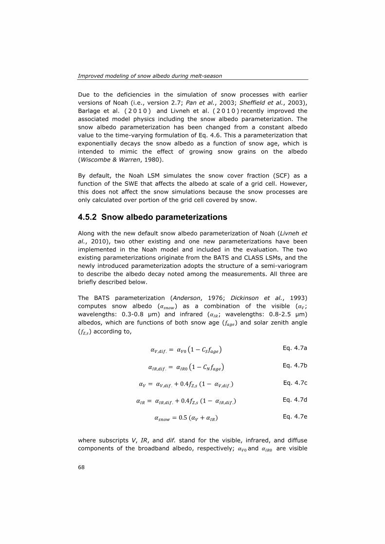
Improved modeling of snow albedo during melt-season
Due to the deficiencies in the simulation of snow processes with earlier versions of Noah (i.e., version 2.7; Pan et al., 2003; Sheffield et al., 2003), Barlage et al. ( 2 0 1 0 ) and Livneh et al. ( 2 0 1 0 ) recently improved the associated model physics including the snow albedo parameterization. The snow albedo parameterization has been changed from a constant albedo value to the time-varying formulation of Eq. 4.6. This a parameterization that exponentially decays the snow albedo as a function of snow age, which is intended to mimic the effect of growing snow grains on the albedo (Wiscombe & Warren, 1980).
By default, the Noah LSM simulates the snow cover fraction (SCF) as a function of the SWE that affects the albedo at scale of a grid cell. However, this does not affect the snow simulations because the snow processes are only calculated over portion of the grid cell covered by snow.
4.5.2 Snow albedo parameterizations
Along with the new default snow albedo parameterization of Noah (Livneh et al., 2010), two other existing and one new parameterizations have been implemented in the Noah model and included in the evaluation. The two existing parameterizations originate from the BATS and CLASS LSMs, and the newly introduced parameterization adopts the structure of a semi-variogram to describe the albedo decay noted among the measurements. All three are briefly described below.
The BATS parameterization (Anderson, 1976; Dickinson et al., 1993) computes snow albedo (𝛼𝑠𝑛𝑜𝑤) as a combination of the visible (𝛼𝑉; wavelengths: 0.3-0.8 µm) and infrared (𝛼𝐼𝑅; wavelengths: 0.8-2.5 µm) albedos, which are functions of both snow age (𝑓𝑎𝑔𝑒) and solar zenith angle (𝑓𝑍,𝑠) according to,
𝛼𝑉,𝑑𝑖𝑓. = 𝛼𝑉0 �1 − 𝐶𝑆𝑓𝑎𝑔𝑒� Eq. 4.7a
𝛼𝐼𝑅,𝑑𝑖𝑓. = 𝛼𝐼𝑅0 �1 − 𝐶𝑁𝑓𝑎𝑔𝑒� Eq. 4.7b
𝛼𝑉 = 𝛼𝑉,𝑑𝑖𝑓. + 0.4𝑓𝑍,𝑠 (1 − 𝛼𝑉,𝑑𝑖𝑓.) Eq. 4.7c
𝛼𝐼𝑅 = 𝛼𝐼𝑅,𝑑𝑖𝑓. + 0.4𝑓𝑍,𝑠 (1 − 𝛼𝐼𝑅,𝑑𝑖𝑓.) Eq. 4.7d
𝛼𝑠𝑛𝑜𝑤 = 0.5 (𝛼𝑉 + 𝛼𝐼𝑅) Eq. 4.7e
where subscripts V, IR, and dif. stand for the visible, infrared, and diffuse components of the broadband albedo, respectively; 𝛼𝑉0 and 𝛼𝐼𝑅0 are visible
68
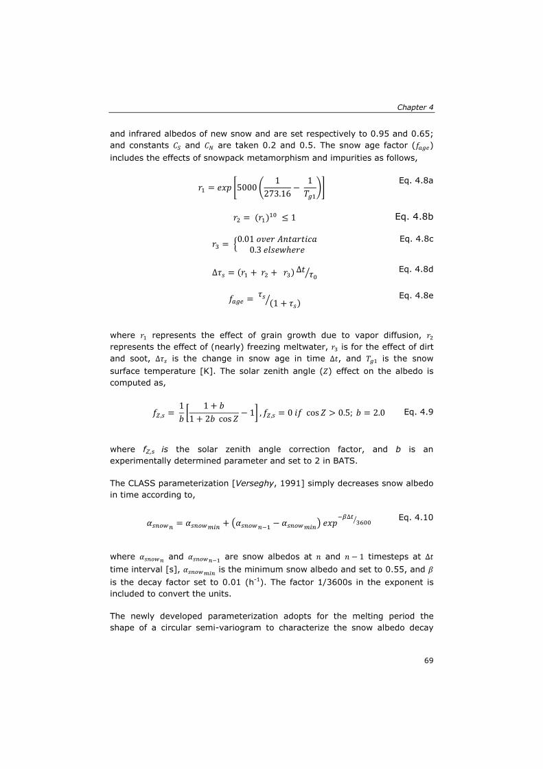
Chapter 4
and infrared albedos of new snow and are set respectively to 0.95 and 0.65; and constants 𝐶𝑆 and 𝐶𝑁 are taken 0.2 and 0.5. The snow age factor (𝑓𝑎𝑔𝑒) includes the effects of snowpack metamorphism and impurities as follows,
𝑟1 = 𝑒𝑥𝑝 �5000 �1
273.16−
1𝑇𝑔1
�� Eq. 4.8a
𝑟2 = (𝑟1)10 ≤ 1 Eq. 4.8b
𝑟3 = �0.01 𝑜𝑣𝑒𝑟 𝐴𝑛𝑡𝑎𝑟𝑡𝑖𝑐𝑎0.3 𝑒𝑙𝑠𝑒𝑤ℎ𝑒𝑟𝑒 Eq. 4.8c
∆𝜏𝑠 = (𝑟1 + 𝑟2 + 𝑟3)∆𝑡 𝜏0� Eq. 4.8d
𝑓𝑎𝑔𝑒 = 𝜏𝑠 (1 + 𝜏𝑠)� Eq. 4.8e
where 𝑟1 represents the effect of grain growth due to vapor diffusion, 𝑟2 represents the effect of (nearly) freezing meltwater, 𝑟3 is for the effect of dirt and soot, ∆𝜏𝑠 is the change in snow age in time ∆𝑡, and 𝑇𝑔1 is the snow surface temperature [K]. The solar zenith angle (𝑍) effect on the albedo is computed as,
𝑓𝑍,𝑠 = 1𝑏�
1 + 𝑏1 + 2𝑏 cos𝑍
− 1� , 𝑓𝑍,𝑠 = 0 𝑖𝑓 cos𝑍 > 0.5; 𝑏 = 2.0 Eq. 4.9
where fZ,s is the solar zenith angle correction factor, and b is an experimentally determined parameter and set to 2 in BATS.
The CLASS parameterization [Verseghy, 1991] simply decreases snow albedo in time according to,
𝛼𝑠𝑛𝑜𝑤𝑛 = 𝛼𝑠𝑛𝑜𝑤𝑚𝑖𝑛 + �𝛼𝑠𝑛𝑜𝑤𝑛−1 − 𝛼𝑠𝑛𝑜𝑤𝑚𝑖𝑛� 𝑒𝑥𝑝−𝛽∆𝑡
3600� Eq. 4.10
where 𝛼𝑠𝑛𝑜𝑤𝑛 and 𝛼𝑠𝑛𝑜𝑤𝑛−1 are snow albedos at 𝑛 and 𝑛 − 1 timesteps at ∆𝑡 time interval [s], 𝛼𝑠𝑛𝑜𝑤𝑚𝑖𝑛 is the minimum snow albedo and set to 0.55, and 𝛽 is the decay factor set to 0.01 (h-1). The factor 1/3600s in the exponent is included to convert the units.
The newly developed parameterization adopts for the melting period the shape of a circular semi-variogram to characterize the snow albedo decay
69
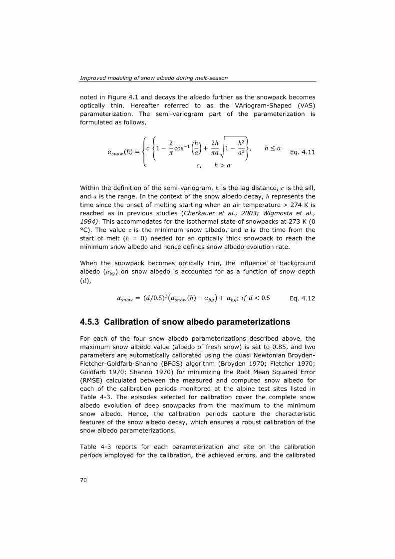
Improved modeling of snow albedo during melt-season
noted in Figure 4.1 and decays the albedo further as the snowpack becomes optically thin. Hereafter referred to as the VAriogram-Shaped (VAS) parameterization. The semi-variogram part of the parameterization is formulated as follows,
𝛼𝑠𝑛𝑜𝑤(ℎ) =
⎩⎨
⎧𝑐 �1 −
2𝜋
cos−1 �ℎ𝑎� +
2ℎ𝜋𝑎
�1 − ℎ2
𝑎2� , ℎ ≤ 𝑎
𝑐, ℎ > 𝑎
Eq. 4.11
Within the definition of the semi-variogram, ℎ is the lag distance, 𝑐 is the sill, and 𝑎 is the range. In the context of the snow albedo decay, ℎ represents the time since the onset of melting starting when an air temperature > 274 K is reached as in previous studies (Cherkauer et al., 2003; Wigmosta et al., 1994). This accommodates for the isothermal state of snowpacks at 273 K (0 °C). The value 𝑐 is the minimum snow albedo, and 𝑎 is the time from the start of melt (ℎ = 0) needed for an optically thick snowpack to reach the minimum snow albedo and hence defines snow albedo evolution rate.
When the snowpack becomes optically thin, the influence of background albedo (𝛼𝑏𝑔) on snow albedo is accounted for as a function of snow depth (𝑑),
𝛼𝑠𝑛𝑜𝑤 = (𝑑/0.5)2�𝛼𝑠𝑛𝑜𝑤(ℎ) − 𝛼𝑏𝑔� + 𝛼𝑏𝑔; 𝑖𝑓 𝑑 < 0.5 Eq. 4.12
4.5.3 Calibration of snow albedo parameterizations
For each of the four snow albedo parameterizations described above, the maximum snow albedo value (albedo of fresh snow) is set to 0.85, and two parameters are automatically calibrated using the quasi Newtonian Broyden-Fletcher-Goldfarb-Shanno (BFGS) algorithm (Broyden 1970; Fletcher 1970; Goldfarb 1970; Shanno 1970) for minimizing the Root Mean Squared Error (RMSE) calculated between the measured and computed snow albedo for each of the calibration periods monitored at the alpine test sites listed in Table 4-3. The episodes selected for calibration cover the complete snow albedo evolution of deep snowpacks from the maximum to the minimum snow albedo. Hence, the calibration periods capture the characteristic features of the snow albedo decay, which ensures a robust calibration of the snow albedo parameterizations.
Table 4-3 reports for each parameterization and site on the calibration periods employed for the calibration, the achieved errors, and the calibrated
70
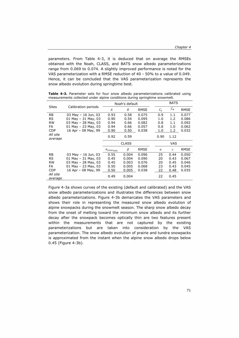
Chapter 4
parameters. From Table 4-3, it is deduced that on average the RMSEs obtained with the Noah, CLASS, and BATS snow albedo parameterizations range from 0.069 to 0.074. A slightly improved performance is noted for the VAS parameterization with a RMSE reduction of 40 - 50% to a value of 0.049. Hence, it can be concluded that the VAS parameterization represents the snow albedo evolution during springtime best.
Table 4-3. Parameter sets for four snow albedo parameterizations calibrated using measurements collected under alpine conditions during springtime snowmelt.
Sites Calibration periods Noah's default BATS
𝐴 𝐵 RMSE 𝐶𝑆 𝐶𝑁 RMSE
RB 03 May – 16 Jun, 03 0.93 0.58 0.075 0.9 1.1 0.077 RS 01 May – 31 May, 03 0.90 0.54 0.095 1.0 1.2 0.086 RW 03 May – 28 May, 03 0.94 0.66 0.082 0.8 1.1 0.092 FA 01 May – 23 May, 03 0.94 0.66 0.057 0.8 1.0 0.062 CDP 16 Apr – 08 May, 99 0.90 0.50 0.038 1.0 1.2 0.032 All site average
0.92 0.59 0.90 1.12
CLASS VAS
𝛼𝑠𝑛𝑜𝑤𝑚𝑖𝑛 𝛽 RMSE 𝑎 𝑐 RMSE
RB 03 May – 16 Jun, 03 0.55 0.004 0.096 25 0.44 0.050 RS 01 May – 31 May, 03 0.45 0.004 0.090 20 0.43 0.067 RW 03 May – 28 May, 03 0.45 0.003 0.076 20 0.45 0.046 FA 01 May – 23 May, 03 0.50 0.005 0.068 23 0.43 0.045 CDP 16 Apr – 08 May, 99 0.50 0.005 0.038 22 0.48 0.035 All site average
0.49 0.004 22 0.45
Figure 4-3a shows curves of the existing (default and calibrated) and the VAS snow albedo parameterizations and illustrates the differences between snow albedo parameterizations. Figure 4-3b demarcates the VAS parameters and shows their role in representing the measured snow albedo evolution of alpine snowpacks during the snowmelt season. The sharp snow albedo decay from the onset of melting toward the minimum snow albedo and its further decay after the snowpack becomes optically thin are two features present within the measurements that are not captured by the existing parameterizations but are taken into consideration by the VAS parameterization. The snow albedo evolution of prairie and tundra snowpacks is approximated from the instant when the alpine snow albedo drops below 0.45 (Figure 4-3b).
71
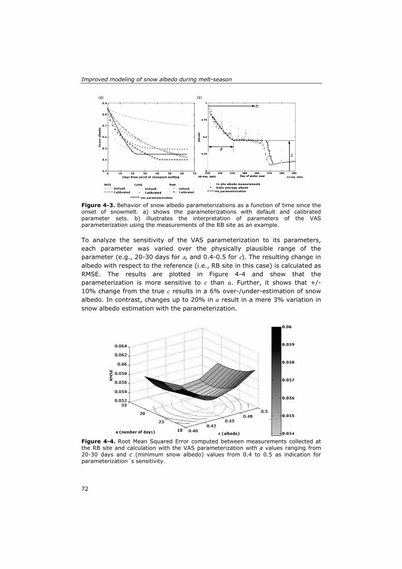
Improved modeling of snow albedo during melt-season
Figure 4-3. Behavior of snow albedo parameterizations as a function of time since the onset of snowmelt. a) shows the parameterizations with default and calibrated parameter sets. b) illustrates the interpretation of parameters of the VAS parameterization using the measurements of the RB site as an example.
To analyze the sensitivity of the VAS parameterization to its parameters, each parameter was varied over the physically plausible range of the parameter (e.g., 20-30 days for a, and 0.4-0.5 for c). The resulting change in albedo with respect to the reference (i.e., RB site in this case) is calculated as RMSE. The results are plotted in Figure 4-4 and show that the parameterization is more sensitive to 𝑐 than 𝑎. Further, it shows that +/- 10% change from the true 𝑐 results in a 6% over-/under-estimation of snow albedo. In contrast, changes up to 20% in 𝑎 result in a mere 3% variation in snow albedo estimation with the parameterization.
Figure 4-4. Root Mean Squared Error computed between measurements collected at the RB site and calculation with the VAS parameterization with a values ranging from 20-30 days and c (minimum snow albedo) values from 0.4 to 0.5 as indication for parameterization´s sensitivity.
72
Chapter 4
4.6 Noah simulations Noah was initialized using the measured land-surface states and driven at a 10 min interval using meteorological forcings measured at the seven sites. The parameters of each snow albedo parameterization are taken as the average of the five alpine sites' calibrated sets (see all site average in Table 4-3). Table 4-4 provides the initial values of the key land-surface states and the duration of the simulations for each site.
Table 4-4. List of land surface states used as model initialization and duration of model runs.
Site SWE (m)
Snow depth (m)
Surface temper-ature (K)
Soil moisture* (m3/m3)
Soil temperature*
(K) Start date End date
RB 1.0 3.0 268 0.4,0.5,0.52 274,274.5,275 30-Mar-03 30-Jun-03
RS 0.63 1.8 269 0.2,0.22,0.25 274,274.5,275 30-Mar-03 20-Jun-03
RW 0.65 2.0 270 0.25,0.2,0.18 274,274.5,275 30-Mar-03 20-Jun-03
FA 0.45 1.7 269 0.29,0.24,0.22 267,268,269 26-Mar-03 20-Jun-03
CDP 0.6 1.58 267 0.32,0.32,0.3 273,274.5,275 28-Feb-99 11-Jun-99
NI 0 0 271 0.06,0.1,0.12 272,272.5,273 20-Feb-03 18-Mar-03
Ivo 0.21 0.65 269 0.15,0.23,0.20 271,271.6,272 24-May-05 15-Jun-05
*Comma separates values of soil moisture and temperature are for the 1st, 2nd, and 3rd soil layers. Italics values are taken from GLDAS (for Ivo and CDP) and NLDAS (for FA). Soil moisture and temperature measurements are made for the three soil layers; the values of the third layer are repeated for the fourth layer.
4.6.1 Snow albedo
Figure 4-5 shows snow albedo simulations for the alpine sites using the four parameterizations. The Noah, BATS, and CLASS parameterizations fail to capture accurately the features of albedo evolution throughout the melting period highlighted in Section 4.4. For all the sites, these parameterizations overestimate snow albedo, which contributes to a prolonged presence of snowpacks. The performance of the new parameterization appears to be much better as is expected based on the results presented in Section 4.5.3. Further, it should be noted that although only observations from second half of the snow season are used for calibration, the obtained parameters are not exclusively valid for this season as also episodes with an increase in snow depth and albedo occur in the selected simulation periods.
73
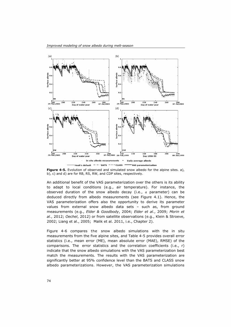
Improved modeling of snow albedo during melt-season
Figure 4-5. Evolution of observed and simulated snow albedo for the alpine sites. a), b), c) and d) are for RB, RS, RW, and CDP sites, respectively.
An additional benefit of the VAS parameterization over the others is its ability to adapt to local conditions (e.g., air temperature). For instance, the observed duration of the snow albedo decay (i.e., 𝑎 parameter) can be deduced directly from albedo measurements (see Figure 4.1). Hence, the VAS parameterization offers also the opportunity to derive its parameter values from external snow albedo data sets – such as, from ground measurements (e.g., Elder & Goodbody, 2004; Elder et al., 2009; Morin et al., 2012; Oechel, 2012) or from satellite observations (e.g., Klein & Stroeve, 2002; Liang et al., 2005; Malik et al. 2011, i.e., Chapter 2).
Figure 4-6 compares the snow albedo simulations with the in situ measurements from the five alpine sites, and Table 4-5 provides overall error statistics (i.e., mean error (ME), mean absolute error (MAE), RMSE) of the comparisons. The error statistics and the correlation coefficients (i.e., r) indicate that the snow albedo simulations with the VAS parameterization best match the measurements. The results with the VAS parameterization are significantly better at 95% confidence level than the BATS and CLASS snow albedo parameterizations. However, the VAS parameterization simulations
74
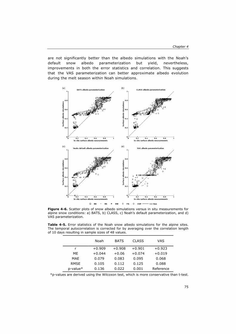
Chapter 4
are not significantly better than the albedo simulations with the Noah’s default snow albedo parameterization but yield, nevertheless, improvements in both the error statistics and correlation. This suggests that the VAS parameterization can better approximate albedo evolution during the melt season within Noah simulations.
Figure 4-6. Scatter plots of snow albedo simulations versus in situ measurements for alpine snow conditions: a) BATS, b) CLASS, c) Noah’s default parameterization, and d) VAS parameterization.
Table 4-5. Error statistics of the Noah snow albedo simulations for the alpine sites. The temporal autocorrelation is corrected for by averaging over the correlation length of 10 days resulting in sample sizes of 48 values.
Noah BATS CLASS VAS
r +0.909 +0.908 +0.901 +0.923 ME +0.044 +0.06 +0.074 +0.019
MAE 0.079 0.083 0.095 0.068 RMSE 0.105 0.112 0.125 0.088
p-value* 0.136 0.022 0.001 Reference
*p-values are derived using the Wilcoxon test, which is more conservative than t-test.
75
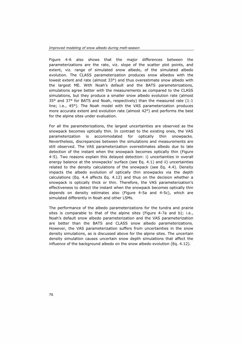
Improved modeling of snow albedo during melt-season
Figure 4-6 also shows that the major differences between the parameterizations are the rate, viz. slope of the scatter plot points, and extent, viz. range of simulated snow albedo, of the simulated albedo evolution. The CLASS parameterization produces snow albedos with the lowest extent and rate (almost 33°) and thus overestimate snow albedo with the largest ME. With Noah’s default and the BATS parameterizations, simulations agree better with the measurements as compared to the CLASS simulations, but they produce a smaller snow albedo evolution rate (almost 35° and 37° for BATS and Noah, respectively) than the measured rate (1:1 line; i.e., 45°). The Noah model with the VAS parameterization produces more accurate extent and evolution rate (almost 42°) and performs the best for the alpine sites under evaluation.
For all the parameterizations, the largest uncertainties are observed as the snowpack becomes optically thin. In contrast to the existing ones, the VAS parameterization is accommodated for optically thin snowpacks. Nevertheless, discrepancies between the simulations and measurements are still observed. The VAS parameterization overestimates albedo due to late detection of the instant when the snowpack becomes optically thin (Figure 4-5). Two reasons explain this delayed detection: i) uncertainties in overall energy balance at the snowpacks’ surface (see Eq. 4.1) and ii) uncertainties related to the density calculations of the snowpack (see Eq. 4.4). Density impacts the albedo evolution of optically thin snowpacks via the depth calculations (Eq. 4.4 affects Eq. 4.12) and thus on the decision whether a snowpack is optically thick or thin. Therefore, the VAS parameterization’s effectiveness to detect the instant when the snowpack becomes optically thin depends on density estimates also (Figure 4-5a and 4-5c), which are simulated differently in Noah and other LSMs.
The performance of the albedo parameterizations for the tundra and prairie sites is comparable to that of the alpine sites (Figure 4-7a and b); i.e., Noah’s default snow albedo parameterization and the VAS parameterization are better than the BATS and CLASS snow albedo parameterizations. However, the VAS parameterization suffers from uncertainties in the snow density simulations, as is discussed above for the alpine sites. The uncertain density simulation causes uncertain snow depth simulations that affect the influence of the background albedo on the snow albedo evolution (Eq. 4.12).
76
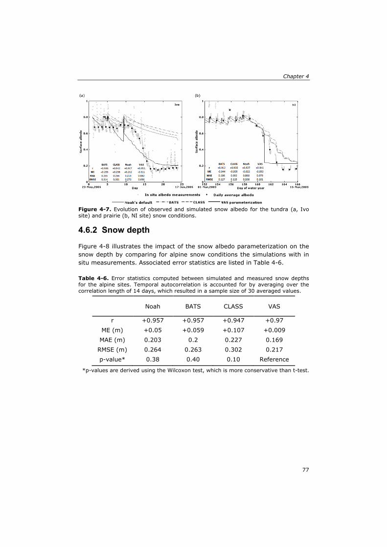
Chapter 4
Figure 4-7. Evolution of observed and simulated snow albedo for the tundra (a, Ivo site) and prairie (b, NI site) snow conditions.
4.6.2 Snow depth
Figure 4-8 illustrates the impact of the snow albedo parameterization on the snow depth by comparing for alpine snow conditions the simulations with in situ measurements. Associated error statistics are listed in Table 4-6.
Table 4-6. Error statistics computed between simulated and measured snow depths for the alpine sites. Temporal autocorrelation is accounted for by averaging over the correlation length of 14 days, which resulted in a sample size of 30 averaged values.
Noah BATS CLASS VAS
r +0.957 +0.957 +0.947 +0.97 ME (m) +0.05 +0.059 +0.107 +0.009 MAE (m) 0.203 0.2 0.227 0.169
RMSE (m) 0.264 0.263 0.302 0.217 p-value* 0.38 0.40 0.10 Reference
*p-values are derived using the Wilcoxon test, which is more conservative than t-test.
77
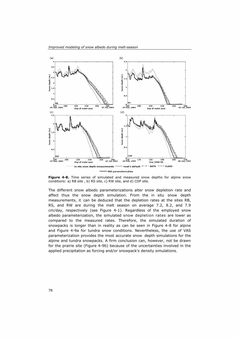
Improved modeling of snow albedo during melt-season
Figure 4-8. Time series of simulated and measured snow depths for alpine snow conditions: a) RB site , b) RS site, c) RW site, and d) CDP site.
The different snow albedo parameterizations alter snow depletion rate and affect thus the snow depth simulation. From the in situ snow depth measurements, it can be deduced that the depletion rates at the sites RB, RS, and RW are during the melt season on average 7.2, 8.2, and 7.9 cm/day, respectively (see Figure 4-1). Regardless of the employed snow albedo parameterization, the simulated snow depletion rates are lower as compared to the measured rates. Therefore, the simulated duration of snowpacks is longer than in reality as can be seen in Figure 4-8 for alpine and Figure 4-9a for tundra snow conditions. Nevertheless, the use of VAS parameterization provides the most accurate snow depth simulations for the alpine and tundra snowpacks. A firm conclusion can, however, not be drawn for the prairie site (Figure 4-9b) because of the uncertainties involved in the applied precipitation as forcing and/or snowpack's density simulations.
78
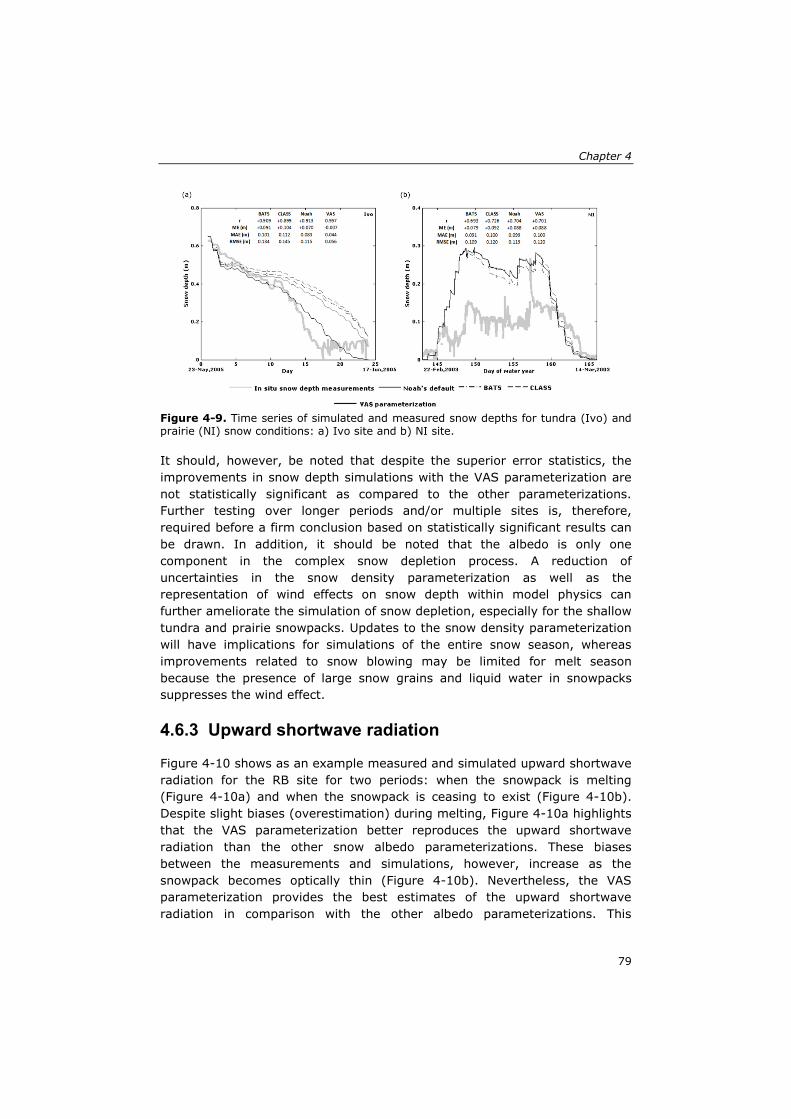
Chapter 4
Figure 4-9. Time series of simulated and measured snow depths for tundra (Ivo) and prairie (NI) snow conditions: a) Ivo site and b) NI site.
It should, however, be noted that despite the superior error statistics, the improvements in snow depth simulations with the VAS parameterization are not statistically significant as compared to the other parameterizations. Further testing over longer periods and/or multiple sites is, therefore, required before a firm conclusion based on statistically significant results can be drawn. In addition, it should be noted that the albedo is only one component in the complex snow depletion process. A reduction of uncertainties in the snow density parameterization as well as the representation of wind effects on snow depth within model physics can further ameliorate the simulation of snow depletion, especially for the shallow tundra and prairie snowpacks. Updates to the snow density parameterization will have implications for simulations of the entire snow season, whereas improvements related to snow blowing may be limited for melt season because the presence of large snow grains and liquid water in snowpacks suppresses the wind effect.
4.6.3 Upward shortwave radiation
Figure 4-10 shows as an example measured and simulated upward shortwave radiation for the RB site for two periods: when the snowpack is melting (Figure 4-10a) and when the snowpack is ceasing to exist (Figure 4-10b). Despite slight biases (overestimation) during melting, Figure 4-10a highlights that the VAS parameterization better reproduces the upward shortwave radiation than the other snow albedo parameterizations. These biases between the measurements and simulations, however, increase as the snowpack becomes optically thin (Figure 4-10b). Nevertheless, the VAS parameterization provides the best estimates of the upward shortwave radiation in comparison with the other albedo parameterizations. This
79
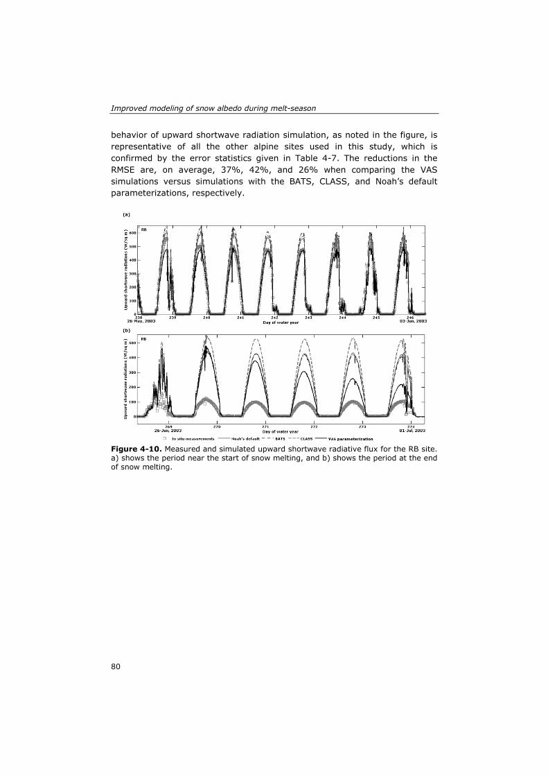
Improved modeling of snow albedo during melt-season
behavior of upward shortwave radiation simulation, as noted in the figure, is representative of all the other alpine sites used in this study, which is confirmed by the error statistics given in Table 4-7. The reductions in the RMSE are, on average, 37%, 42%, and 26% when comparing the VAS simulations versus simulations with the BATS, CLASS, and Noah’s default parameterizations, respectively.
Figure 4-10. Measured and simulated upward shortwave radiative flux for the RB site. a) shows the period near the start of snow melting, and b) shows the period at the end of snow melting.
80
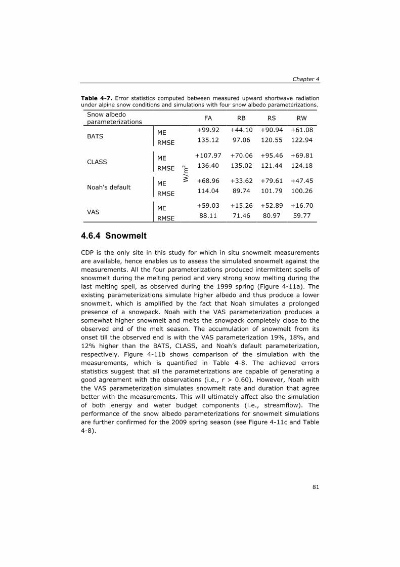
Chapter 4
Table 4-7. Error statistics computed between measured upward shortwave radiation under alpine snow conditions and simulations with four snow albedo parameterizations.
Snow albedo parameterizations
FA RB RS RW
BATS ME
W/m
2
+99.92 +44.10 +90.94 +61.08
RMSE 135.12 97.06 120.55 122.94
CLASS ME +107.97 +70.06 +95.46 +69.81
RMSE 136.40 135.02 121.44 124.18
Noah's default ME +68.96 +33.62 +79.61 +47.45
RMSE 114.04 89.74 101.79 100.26
VAS ME +59.03 +15.26 +52.89 +16.70
RMSE 88.11 71.46 80.97 59.77
4.6.4 Snowmelt
CDP is the only site in this study for which in situ snowmelt measurements are available, hence enables us to assess the simulated snowmelt against the measurements. All the four parameterizations produced intermittent spells of snowmelt during the melting period and very strong snow melting during the last melting spell, as observed during the 1999 spring (Figure 4-11a). The existing parameterizations simulate higher albedo and thus produce a lower snowmelt, which is amplified by the fact that Noah simulates a prolonged presence of a snowpack. Noah with the VAS parameterization produces a somewhat higher snowmelt and melts the snowpack completely close to the observed end of the melt season. The accumulation of snowmelt from its onset till the observed end is with the VAS parameterization 19%, 18%, and 12% higher than the BATS, CLASS, and Noah’s default parameterization, respectively. Figure 4-11b shows comparison of the simulation with the measurements, which is quantified in Table 4-8. The achieved errors statistics suggest that all the parameterizations are capable of generating a good agreement with the observations (i.e., r > 0.60). However, Noah with the VAS parameterization simulates snowmelt rate and duration that agree better with the measurements. This will ultimately affect also the simulation of both energy and water budget components (i.e., streamflow). The performance of the snow albedo parameterizations for snowmelt simulations are further confirmed for the 2009 spring season (see Figure 4-11c and Table 4-8).
81
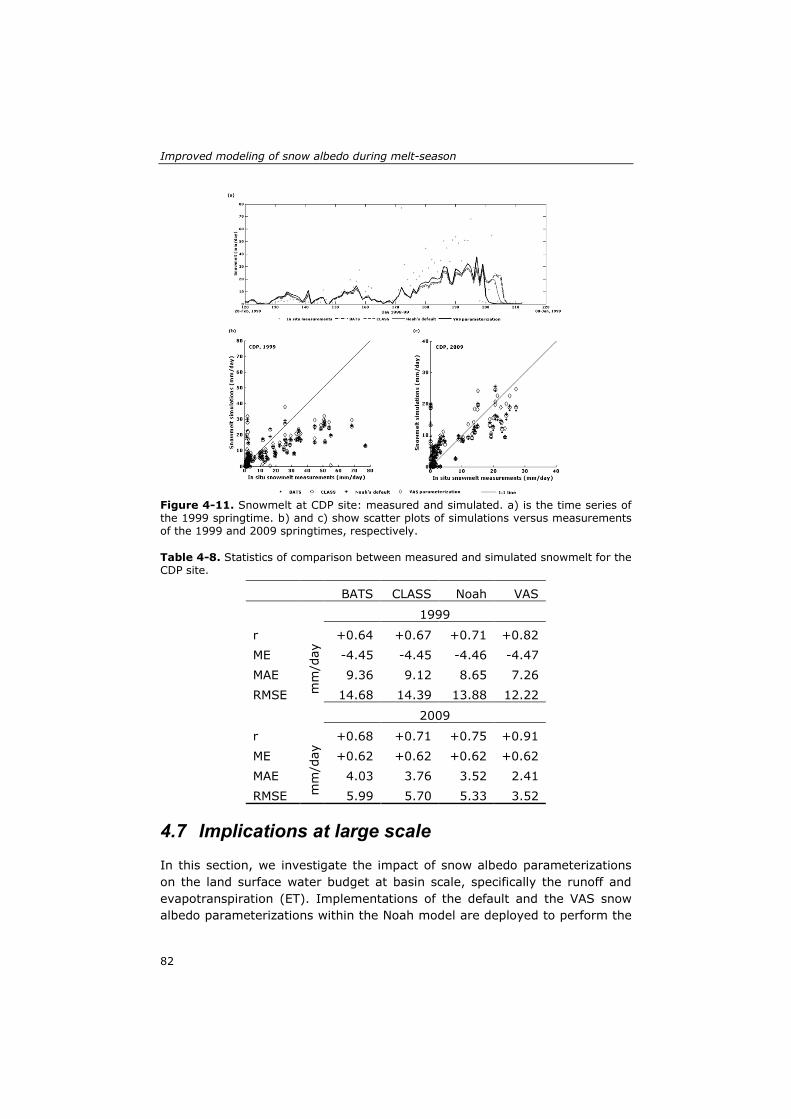
Improved modeling of snow albedo during melt-season
Figure 4-11. Snowmelt at CDP site: measured and simulated. a) is the time series of the 1999 springtime. b) and c) show scatter plots of simulations versus measurements of the 1999 and 2009 springtimes, respectively.
Table 4-8. Statistics of comparison between measured and simulated snowmelt for the CDP site.
BATS CLASS Noah VAS
1999
r
mm
/day
+0.64 +0.67 +0.71 +0.82 ME -4.45 -4.45 -4.46 -4.47 MAE 9.36 9.12 8.65 7.26 RMSE 14.68 14.39 13.88 12.22
2009
r
mm
/day
+0.68 +0.71 +0.75 +0.91 ME +0.62 +0.62 +0.62 +0.62 MAE 4.03 3.76 3.52 2.41 RMSE 5.99 5.70 5.33 3.52
4.7 Implications at large scale In this section, we investigate the impact of snow albedo parameterizations on the land surface water budget at basin scale, specifically the runoff and evapotranspiration (ET). Implementations of the default and the VAS snow albedo parameterizations within the Noah model are deployed to perform the
82
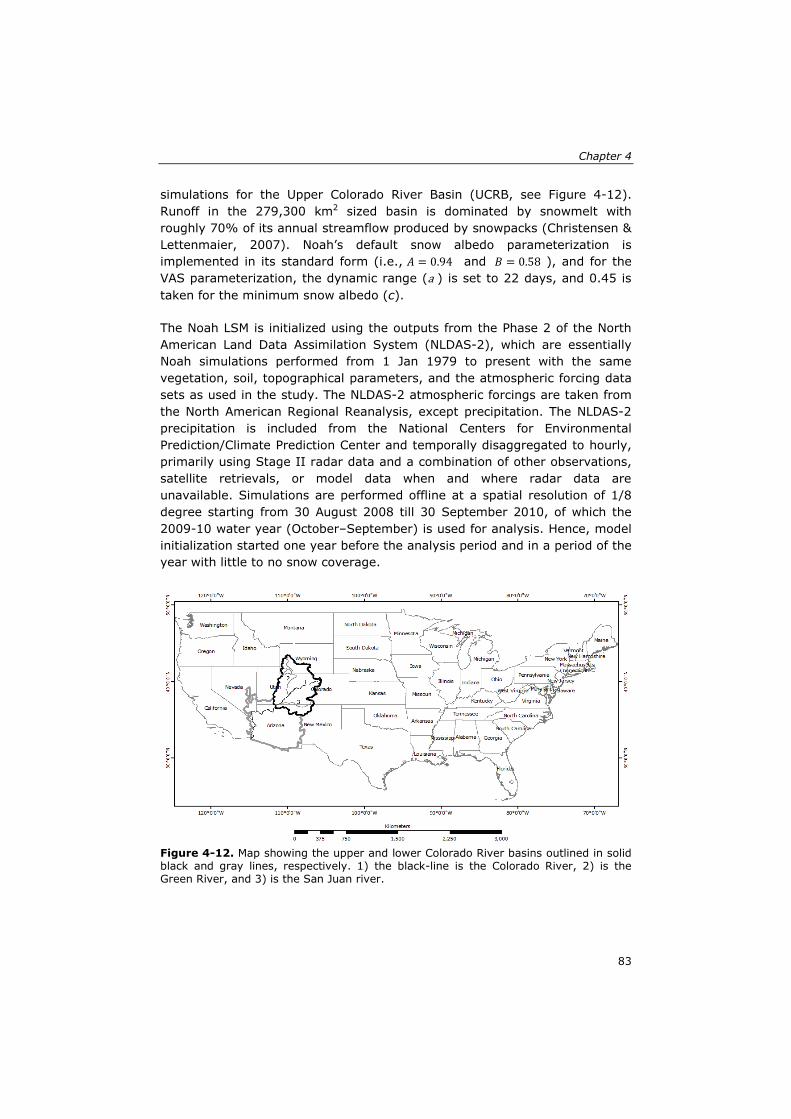
Chapter 4
simulations for the Upper Colorado River Basin (UCRB, see Figure 4-12). Runoff in the 279,300 km2 sized basin is dominated by snowmelt with roughly 70% of its annual streamflow produced by snowpacks (Christensen & Lettenmaier, 2007). Noah’s default snow albedo parameterization is implemented in its standard form (i.e., 𝐴 = 0.94 and 𝐵 = 0.58 ), and for the VAS parameterization, the dynamic range (a ) is set to 22 days, and 0.45 is taken for the minimum snow albedo (c).
The Noah LSM is initialized using the outputs from the Phase 2 of the North American Land Data Assimilation System (NLDAS-2), which are essentially Noah simulations performed from 1 Jan 1979 to present with the same vegetation, soil, topographical parameters, and the atmospheric forcing data sets as used in the study. The NLDAS-2 atmospheric forcings are taken from the North American Regional Reanalysis, except precipitation. The NLDAS-2 precipitation is included from the National Centers for Environmental Prediction/Climate Prediction Center and temporally disaggregated to hourly, primarily using Stage II radar data and a combination of other observations, satellite retrievals, or model data when and where radar data are unavailable. Simulations are performed offline at a spatial resolution of 1/8 degree starting from 30 August 2008 till 30 September 2010, of which the 2009-10 water year (October–September) is used for analysis. Hence, model initialization started one year before the analysis period and in a period of the year with little to no snow coverage.
Figure 4-12. Map showing the upper and lower Colorado River basins outlined in solid black and gray lines, respectively. 1) the black-line is the Colorado River, 2) is the Green River, and 3) is the San Juan river.
83
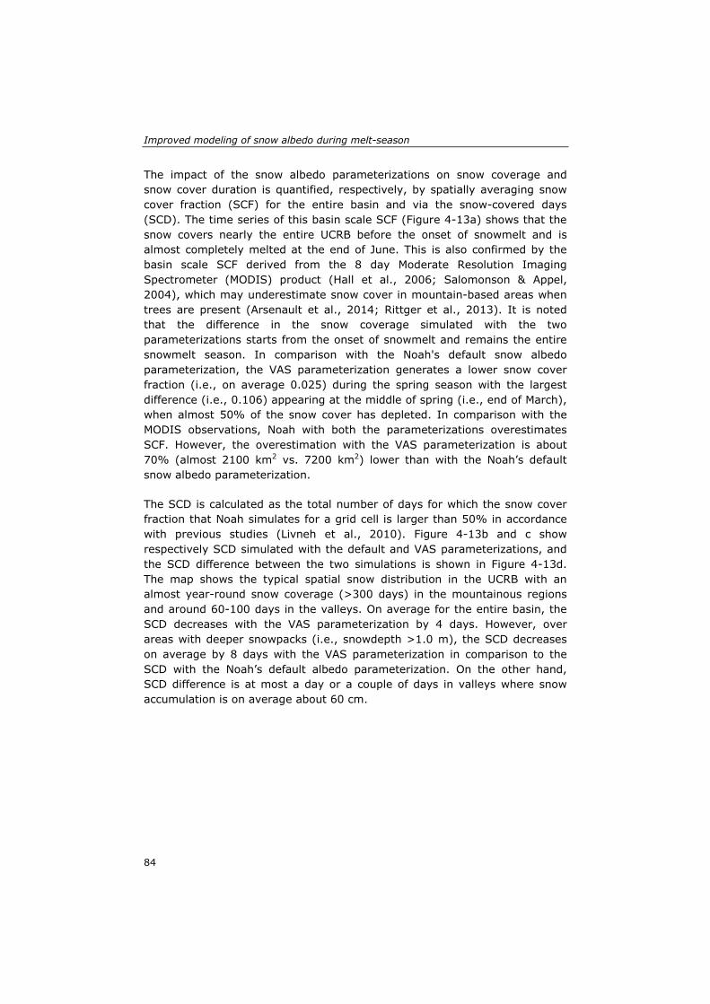
Improved modeling of snow albedo during melt-season
The impact of the snow albedo parameterizations on snow coverage and snow cover duration is quantified, respectively, by spatially averaging snow cover fraction (SCF) for the entire basin and via the snow-covered days (SCD). The time series of this basin scale SCF (Figure 4-13a) shows that the snow covers nearly the entire UCRB before the onset of snowmelt and is almost completely melted at the end of June. This is also confirmed by the basin scale SCF derived from the 8 day Moderate Resolution Imaging Spectrometer (MODIS) product (Hall et al., 2006; Salomonson & Appel, 2004), which may underestimate snow cover in mountain-based areas when trees are present (Arsenault et al., 2014; Rittger et al., 2013). It is noted that the difference in the snow coverage simulated with the two parameterizations starts from the onset of snowmelt and remains the entire snowmelt season. In comparison with the Noah's default snow albedo parameterization, the VAS parameterization generates a lower snow cover fraction (i.e., on average 0.025) during the spring season with the largest difference (i.e., 0.106) appearing at the middle of spring (i.e., end of March), when almost 50% of the snow cover has depleted. In comparison with the MODIS observations, Noah with both the parameterizations overestimates SCF. However, the overestimation with the VAS parameterization is about 70% (almost 2100 km2 vs. 7200 km2) lower than with the Noah’s default snow albedo parameterization.
The SCD is calculated as the total number of days for which the snow cover fraction that Noah simulates for a grid cell is larger than 50% in accordance with previous studies (Livneh et al., 2010). Figure 4-13b and c show respectively SCD simulated with the default and VAS parameterizations, and the SCD difference between the two simulations is shown in Figure 4-13d. The map shows the typical spatial snow distribution in the UCRB with an almost year-round snow coverage (>300 days) in the mountainous regions and around 60-100 days in the valleys. On average for the entire basin, the SCD decreases with the VAS parameterization by 4 days. However, over areas with deeper snowpacks (i.e., snowdepth >1.0 m), the SCD decreases on average by 8 days with the VAS parameterization in comparison to the SCD with the Noah’s default albedo parameterization. On the other hand, SCD difference is at most a day or a couple of days in valleys where snow accumulation is on average about 60 cm.
84
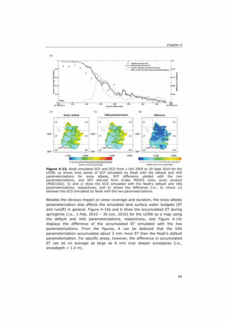
Chapter 4
Figure 4-13. Noah simulated SCF and SCD from 1-Oct 2009 to 30 Sept 2010 for the UCRB. a) shows time series of SCF simulated by Noah with the default and VAS parameterizations for snow albedo, SCF difference yielded with the two parameterizations, and SCF derived from 8-day MODIS snow cover product (MOD10A2). b) and c) show the SCD simulated with the Noah’s default and VAS parameterizations, respectively, and d) shows the difference [i.e., b) minus c)] between the SCD simulated by Noah with the two parameterizations.
Besides the obvious impact on snow coverage and duration, the snow albedo parameterization also affects the simulated land surface water budgets (ET and runoff) in general. Figure 4-14a and b show the accumulated ET during springtime (i.e., 1-Feb, 2010 – 30-Jun, 2010) for the UCRB as a map using the default and VAS parameterizations, respectively, and Figure 4-14c displays the difference of the accumulated ET simulated with the two parameterizations. From the figures, it can be deduced that the VAS parameterization accumulates about 3 mm more ET than the Noah’s default parameterization. For specific areas, however, the difference in accumulated ET can be on average as large as 8 mm over deeper snowpacks (i.e., snowdepth > 1.0 m).
85
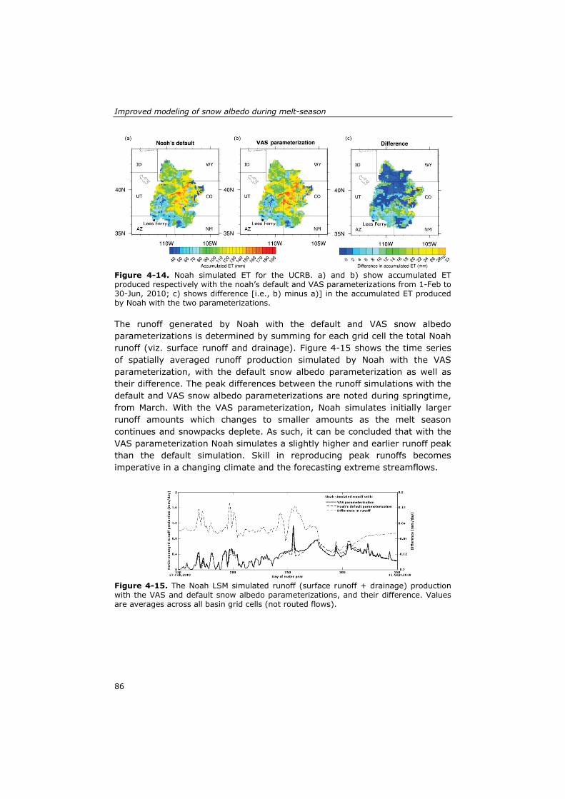
Improved modeling of snow albedo during melt-season
Figure 4-14. Noah simulated ET for the UCRB. a) and b) show accumulated ET produced respectively with the noah’s default and VAS parameterizations from 1-Feb to 30-Jun, 2010; c) shows difference [i.e., b) minus a)] in the accumulated ET produced by Noah with the two parameterizations.
The runoff generated by Noah with the default and VAS snow albedo parameterizations is determined by summing for each grid cell the total Noah runoff (viz. surface runoff and drainage). Figure 4-15 shows the time series of spatially averaged runoff production simulated by Noah with the VAS parameterization, with the default snow albedo parameterization as well as their difference. The peak differences between the runoff simulations with the default and VAS snow albedo parameterizations are noted during springtime, from March. With the VAS parameterization, Noah simulates initially larger runoff amounts which changes to smaller amounts as the melt season continues and snowpacks deplete. As such, it can be concluded that with the VAS parameterization Noah simulates a slightly higher and earlier runoff peak than the default simulation. Skill in reproducing peak runoffs becomes imperative in a changing climate and the forecasting extreme streamflows.
Figure 4-15. The Noah LSM simulated runoff (surface runoff + drainage) production with the VAS and default snow albedo parameterizations, and their difference. Values are averages across all basin grid cells (not routed flows).
86
Chapter 4
4.8 Conclusion In this study, we examine observed snow albedo decay during springtime and assess the performance of the Noah, BATS, and CLASS land surface models (LSM) snow albedo parameterizations. The latter two parameterizations were implemented within the overall model physics of the Noah LSM. The Noah LSM was run using the three parameterizations across the snowmelt seasons characterized at seven sites, of which five are from alpine, one from tundra, and one from prairie snow conditions. The comparison of the simulated snow albedo evolution with the in situ measurements shows that the parameterizations adopted by Noah, BATS, and CLASS are only able to simulate an albedo decay but do not reproduce its stabilization at the minimum value of optically thick snowpacks within the observed time. This limitation directly affects the rate of the snow albedo decay and total range of simulated snow albedo values. At present, the above mentioned parameterizations overestimate snow albedo during the melt season, which reduces the Noah simulated melt rate and extends the simulated snowpack duration.
Based upon these observations, we propose a new parameterization for simulating the snow albedo during the melting period that adopts the shape of a semi-variogram when the snowpack remains optically thick and decreases the albedo further via a weighted average of snow and land surface (background) albedos as a function of snow depth when the snowpack becomes optically thin. The variogram-shaped (VAS) snow albedo parameterization has been implemented in the Noah LSM and employed for simulating the snow processes over alpine, tundra, and prairie snowpacks. Apart from an improved snow albedo simulation, the VAS parameterization also has positive impacts on the simulation of snow depth, melt rate, snowpack duration, and upward shortwave radiation. Improvements obtained with the VAS parameterization consist essentially of a lower deep snowpack albedo for the melt season that accelerates the melt rate and associated surface hydrological processes.
In spite of these improvements, uncertainties still exist particularly during episodes with optically thin snowpacks (e.g., snow density, atmospheric forcings). These make the impact of the VAS parameterization on simulations for the shallow prairie snowpacks less notable. Therefore, further studies are required to optimize the snow albedo modeling for prairie snowpacks and, arguably, to improve the snow density parameterization.
The impact of the snow albedo is also assessed at a large scale for the Upper Colorado River Basin by comparing the Noah simulations with the VAS and default parameterizations. Noah simulates, in line with the results obtained at
87
Improved modeling of snow albedo during melt-season
plot scale, with the VAS parameterization a shorter snowpack duration. Notably, the fractional snow coverage simulated with the VAS parameterization agrees better with the snow cover observed by MODIS. This difference in the simulation of the snowpack states increases the evapotranspiration during the selected spring season of 2010 and affects the timing and magnitude of the runoff production. Noah simulates with the VAS parameterization a higher runoff peak in springtime and smaller volumes in the summer season.
The improvement in snow albedo simulation with the VAS parameterization has demonstrated the potential to improve the simulation of the land-surface states, energy, and water fluxes at the land-atmosphere interface, which may also positively impact the simulation of atmospheric processes when operated in a coupled system. However, additional testing over longer periods (i.e., multiple snow seasons) at different spatial resolutions, climatic regions, and physiographic conditions (i.e., forest-covered areas) is required to draw firm conclusions about the impact of different snow albedo parameterizations in simulating the snowpack properties and to validate large-scale simulations. The VAS parameterization is numerically efficient, and its parameters are derived from albedo measurements, which can also be obtained via satellite observations. The latter is particularly relevant in view of the recent launch of Landsat-8 and the upcoming Sentinel-2 mission with its launch date scheduled in 2014.
88
5 Assimilation of satellite-observed snow albedo in a land surface model
Abstract
This chapter assesses the impact of assimilating satellite-observed snow albedo on the Noah land surface model (LSM)-simulated fluxes and snow properties. A direct insertion technique is developed to assimilate snow albedo into Noah and is applied to three intensive study areas in North Park (Colorado) that are part of the 2002/03 Cold Land Processes Field Experiment (CLPX). The assimilated snow albedo products are 1) the standard Moderate Resolution Imaging Spectrometer (MODIS) product (MOD10A1) and 2) retrievals from MODIS observations with the recently developed Pattern-Based Semi-empirical (PASS) approach. The performance of the Noah simulations, with and without assimilation, is evaluated using the in situ measurements of snow albedo, upward shortwave radiation, and snow depth. The results show that simulations with albedo assimilation agree better with the measurements. However, because of the limited impact of snow albedo updates after subsequent snowfall, the mean (or seasonal) error statistics decrease significantly for only two of the three CLPX sites. Though the simulated snow depth and duration for the snow season benefit from the assimilation, the greatest improvements are found in the simulated upward shortwave radiation, with root mean squared errors reduced by about 30%. As such, this chapter demonstrates that assimilation of satellite-observed snow albedo can improve LSM simulations, which may positively affect the representation of hydrological and surface energy budget processes in runoff and numerical weather prediction models.
Based on
Malik, M. J., R. van der Velde, Z. Vekerdy, and Z. Su (2012). Assimilation of Satellite-Observed Snow Albedo in a Land Surface Model. Journal of Hydrometeorology, 13(3), 1119-1130.
89
Assimilation of satellite-observed snow albedo in a land surface model
5.1 Introduction The albedo of snow affects the shortwave (SW; spectral range from 0.3 to 2.5 μm) radiativeflux at the land–atmosphere interface and is, therefore, important for calculation of surface energy as well as mass (water) budgets. During snow cover periods, however, the albedo changes because of snow metamorphic processes [e.g., melt–freeze cycles, wind redistribution, sublimation, and vapor diffusion (DeWalle & Rango 2008)]. It is generally understood that the albedo decreases as the snow grain size increases (Wiscombe & Warren 1980). Livneh et al. (2010) recently included the effect of this albedo decay within the cold season processes component of the Noah land surface model (LSM; Ek et al. 2003). The authors incorporated an exponential decay as a function of snow age. Nevertheless, uncertainties in the snow albedo simulations still exist because of the fact that the rate of snow albedo decay depends on the dynamics of atmosphere near the surface, which is ignored (Chapter 4). Moreover, LSM simulations are also subject to other sources of uncertainties, such as forcings, parameterization, initialization, and spatial discretization of the land surface.
On the other hand, the snow albedo can be observed remotely with satellite sensors. Several approaches exist for snow albedo retrieval from remote sensing observations. These include lookup table approaches (Painter et al. 2009; Stamnes et al. 2007), empirical approaches based on anisotropic reflectance function (ARF), (Klein & Stroeve 2002; Liang et al. 2005), and (semi) analytical approaches (Kokhanovsky & Zege 2004; Lyapustin et al. 2009; Tedesco & Kokhanovsky 2007) based on Lambertian reflectance for the snow albedo retrieval. Recently, Malik et al. (2011, i.e., Chapter 2) presented a Pattern-Based Semi-empirical (PASS) approach, which exploits triangular variability pattern of albedo and reflectance formed because of varying sun-sensor geometry to retrieve snow albedo. The authors obtained with this method a 50% better agreement with in situ measurements as compared to the Moderate Resolution Imaging Spectroradiometer (MODIS) product (i.e., MOD10A1 daily snow albedo estimates; Klein & Stroeve 2002).
Integration of these satellite-based products within LSMs, such as Noah, can assist in further reducing the uncertainties discussed above. Several successful examples can be found on the assimilation of snow variables. For example, Rodell and Houser (2004) adjusted snow water equivalent (SWE) using MODIS fractional snow coverage (FSC) information when and where the model and MODIS observation differs. Similarly, Andreadis and Lettenmaier (2006) and Zaitchik and Rodell (2009) updated SWE from MODIS FSC estimates using an ensemble Kalman filter (EnKF) and rule-based direct insertion (DI), respectively. However, the usage of satellite-based snow albedo products has so far not yet been explored for assimilation.
90
Chapter 5
The objective of the study is to assess the impact of assimilating snow albedo estimates on the fluxes and snow properties simulated by the Noah LSM. We focus on reducing the uncertainty in Noah simulations by assimilating the snow albedo via the DI technique. Because DI assumes that the observations ingested into the modeling system are error free, three snow albedo products with different inherent uncertainties have been selected for assimilation—namely, the ground measurements and the MODIS-based snow albedo products from Malik et al. (2011, i.e., Chapter 2) and the standard MOD10A1. As such, the assumption of error-free observations is quantified by updating Noah with observations of different inherent uncertainties.
Physics describing the snow processes in the LSM have recently been improved (Barlage et al. 2010; Livneh et al. 2010; Wang et al. 2010). Hence, the focus is on the assessment of the assimilation impact rather than on improving the model physics. The 2002/03 winter season measured during the Cold Land Processes Field Experiment (CLPX) is selected as a test bed because it includes remote sensing observations as well as the in situ measurements needed to force and to validate Noah. The structure of this chapter is as follows: Section 5.2 describes the study area and the ground measurements. Section 5.3 describes the satellite-based snow albedo products used for assimilation. Section 5.4 presents the relevant cold season processes included in the Noah LSM and the control (or open loop) simulations (i.e., without snow albedo updates). In Section 5.5, the data assimilation procedure is described and the results are presented. Finally, some concluding remarks are given in Section 5.6.
5.2 CLPX
5.2.1 Study area
During the CLPX 2002/03 winter season, data were collected at three mesocell study areas (MSA) in Colorado, each covering an area of about 25 × 25 km2. In situ measurements within the MSAs were collected at three 1-km2 intensive study areas (ISA). We selected for our study the sites with low-topographic relief and without forest to minimize the uncertainties in satellite-observed snow albedo. The utilized ISAs are Illinois River [North Park, Illinois River (NI); 40.6954°N, 106.2545°W; World Geodetic System 1984 (WGS 84) ellipsoid model], Michigan River [North Park, Michigan River (NM); 40.6450°N, 106.1809°W; WGS 84], and Potter Creek [North Park, Potter Creek (NP); 40.6677°N, 106.3232°W; WGS 84). All the sites are located within the North Park MSA.
The North Park MSA has very low relief and grassland dominates the land cover. The MSA has a mean elevation of 2499 m and the predominant soil
91
Assimilation of satellite-observed snow albedo in a land surface model
texture is sandy loam. Snowpacks at North Park can be classified as prairie and tundra covers (Sturm et al. 1995), which are representative for about 53% of seasonally snow-covered areas globally. The soils are typically frozen during the winter season because of the shallow and windswept snow cover. More information about the North Park MSA and its ISAs can be found at http://www.nohrsc.nws.gov/~cline/clpx.html (accessed 4 December, 2013).
5.2.2 Ground measurements
The field measurements, needed to run (force and initialize) as well as to validate Noah, were collected at the CLPX meteorological towers in the center of the ISAs named: NI, NM, and NP. Soil moisture and soil and skin temperature measurements are used for the model initialization. The CLPX wind speed, wind direction, air temperature, relative humidity, atmospheric pressure, and short- and longwave downward radiation are used as forcings. The atmospheric variables were recorded at a 10-min interval 2 m above the ground surface in the MSA (Elder & Goodbody 2004; Elder et al. 2009). Precipitation inputs are obtained from the North American Land Data Assimilation System version 2 (NLDAS-2; Ek et al. 2011; Xia et al. 2011), which is an hourly merged gauge-radar product at ⅛° (or 12.5 km) spatial resolution.
The meteorological towers were also equipped with an acoustic sounder for measuring snow depths with an estimated accuracy of ±1.0 cm (Elder et al. 2009). These snow depths, the upward shortwave radiation, and the albedo derived from the measurements made by net radiometers are used to evaluate Noah’s performance with and without the snow albedo assimilation. Details of the instruments employed during the CLPX to collect the measurements utilized for this study are provided in Table 5-1.
92
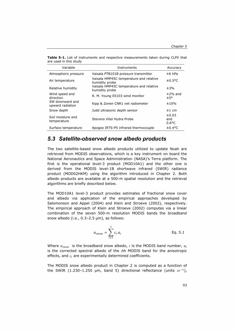
Chapter 5
Table 5-1. List of instruments and respective measurements taken during CLPX that are used in this study
Variable Instruments Accuracy
Atmospheric pressure Vaisala PTB101B pressure transmitter ±6 hPa
Air temperature Vaisala HMP45C temperature and relative humidity probe ±0.5°C
Relative humidity Vaisala HMP45C temperature and relative humidity probe ±3%
Wind speed and direction R. M. Young 05103 wind monitor ±2% and
±5° SW downward and upward radiation Kipp & Zonen CNR1 net radiometer ±10%
Snow depth Judd ultrasonic depth sensor ±1 cm
Soil moisture and temperature Stevens Vitel Hydra Probe
±0.03 and 0.6°C
Surface temperature Apogee IRTS-P5 infrared thermocouple ±0.4°C
5.3 Satellite-observed snow albedo products The two satellite-based snow albedo products utilized to update Noah are retrieved from MODIS observations, which is a key instrument on board the National Aeronautics and Space Administration (NASA)’s Terra platform. The first is the operational level-3 product (MOD10A1) and the other one is derived from the MODIS level-1B shortwave infrared (SWIR) radiance product (MOD02HKM) using the algorithm introduced in Chapter 2. Both albedo products are available at a 500-m spatial resolution and the retrieval algorithms are briefly described below.
The MOD10A1 level-3 product provides estimates of fractional snow cover and albedo via application of the empirical approaches developed by Salomonson and Appel (2004) and Klein and Stroeve (2002), respectively. The empirical approach of Klein and Stroeve (2002) computes via a linear combination of the seven 500-m resolution MODIS bands the broadband snow albedo (i.e., 0.3–2.5 μm), as follows:
𝛼𝑠𝑛𝑜𝑤 = �𝑐𝑖
7
𝑖=1
𝑎𝑖 Eq. 5.1
Where 𝛼𝑠𝑛𝑜𝑤 is the broadband snow albedo, 𝑖 is the MODIS band number, 𝑎𝑖 is the corrected spectral albedo of the 𝑖th MODIS band for the anisotropic effects, and 𝑐𝑖 are experimentally determined coefficients.
The MODIS snow albedo product in Chapter 2 is computed as a function of the SWIR (1.230–1.250 μm, band 5) directional reflectance (units 𝑠𝑟−1),
93
Assimilation of satellite-observed snow albedo in a land surface model
derived from the MOD02HKM radiance [units W (m2 μm sr)−1]. The developed PASS approach retrieves the spectral snow albedo from the observed reflectance, while accounting for the directional effects due to varying sun-sensor geometry represented by a right triangular pattern. The base (𝑏) of this triangle is defined as a function of the solar zenith and the height (ℎ) is given by the scattering angle, as follows:
𝑏 = 0.29 − � �(1.4𝑒 − 6 𝜃𝑜2) + (3.6𝑒 − 6 𝜃𝑜) + 0.00061�𝑑𝜃𝑜𝜃𝑜′
0 Eq. 5.2
ℎ = 0.43 − � ((−1.9𝑒 − 8 𝜃𝑠𝑐𝑎3 ) + (7.9𝑒 − 6 𝜃𝑠𝑐𝑎2 ) − (0.0011 𝜃𝑠𝑐𝑎)𝜃𝑠𝑐𝑎′
40+ 0.05) 𝑑𝜃𝑠𝑐𝑎
Eq. 5.3
where 𝜃𝑜 and 𝜃𝑠𝑐𝑎 are incident and scattering angles, respectively, and 𝜃𝑜′ and 𝜃𝑠𝑐𝑎′ are incident and scattering angles used for the radiance measurement. The 𝑏 and ℎ in combination with the directional reflectance provide the spectral albedo (𝑎𝑠𝑝), which is converted into the broadband snow albedo as follows:
𝛼𝑛𝑖𝑟 = 1.1 𝑎𝑠𝑝3 − 1.1𝑎𝑠𝑝2 + 0.86𝑎𝑠𝑝 + 0.098 Eq. 5.4 𝛼𝑠𝑛𝑜𝑤 = 𝛼𝑣𝑖𝑠𝑓𝑣𝑖𝑠 + 𝛼𝑛𝑖𝑟(1 − 𝑓𝑣𝑖𝑠) Eq. 5.5
where 𝛼𝑛𝑖𝑟 is near-infrared albedo, 𝛼𝑣𝑖𝑠 is visible albedo, 𝑓𝑣𝑖𝑠 is the visible light fraction of shortwave downwelling radiation, and 𝛼𝑠𝑛𝑜𝑤 is broadband snow albedo.
Stroeve et al. (2006) evaluated the Terra MOD10A1 product with in situ measurements collected over Greenland and reported an overall root-mean-square error (RMSE) of 0.067 and correlation coefficient (r) of 0.79. Malik et al. (2011, i.e., Chapter 2) obtained similar results (i.e., RMSE of 0.064 and r = 0.6), with MOD10A1 over the North Park CLPX sites and the Namco Lake on the Tibetan Plateau. The error statistics reported in Malik et al. (2011, i.e., Chapter 2) for the PASS approach are, with a RMSE = 0.03 and a r = 0.8 for the CLPX’s North Park and Tibetan Plateau sites, better than the MOD10A1 product.
5.4 Noah snow process simulations
5.4.1 Model physics
Noah (Ek et al. 2003; Mitchell 2005) is a one-dimensional (i.e., fluxes are not exchanged across the model grid) process model that can operate either in coupled mode to a general circulation model (GCM) or an offline mode. Noah
94
Chapter 5
represents the snowpack as a single layer, for which the snow states are defined (i.e., albedo, density, depth, and water equivalent). In this study, we use the most recent public release (version 3.3), in which significant improvements have been made to the snow process physics (Barlage et al. 2010; Wang et al. 2010).
Most relevant for this study is the implementation of a time-varying snow albedo formulation reported in Livneh et al. (2010). The modified Noah simulates the snow albedo (𝛼𝑠𝑛𝑜𝑤) as the maximum broadband snow albedo (𝛼𝑚𝑎𝑥) reduced by a time-dependent decay factor, which is reset to 1 on snowfall, as follows:
𝛼𝑠𝑛𝑜𝑤 = 𝛼𝑚𝑎𝑥𝐴𝐵𝑡 Eq. 5.6
where 𝐴 and 𝐵 are constants defined differently for dry and wet snowpacks, and 𝑡 is the time in days since the last snowfall. This formulation is adopted from Distributed Hydrology Soil Vegetation Model (DHSVM; Wigmosta et al. 1994) and has also been implemented in the Variable Infiltration Capacity (VIC) LSM (Cherkauer et al. 2003).
The exponential decay with time mimics the snow metamorphism, causing changes in the snow grain size and, as a result, the albedo. As the albedo is a variable in the surface energy budget, this modification alters the mass–water fluxes at the snow surface, affecting SWE simulations and, indirectly, snow depth. Also noteworthy is the improved snow-specific density formulation near the melting point, which impacts the snow depth simulations via its calculation as a ratio of the SWE over the snow-specific density.
5.4.2 Open-loop simulation
To provide a reference for the following sections, Noah is run without data assimilation for the NI ISA over the period of 26 October 2002–15 March 2003 using the atmospheric forcings described in Section 5.2.2. The initialization and parameterizations representative for the NI site are obtained from the CLPX measurements and NLDAS.
Table 5-2 provides the adopted initial states and parameters.
95
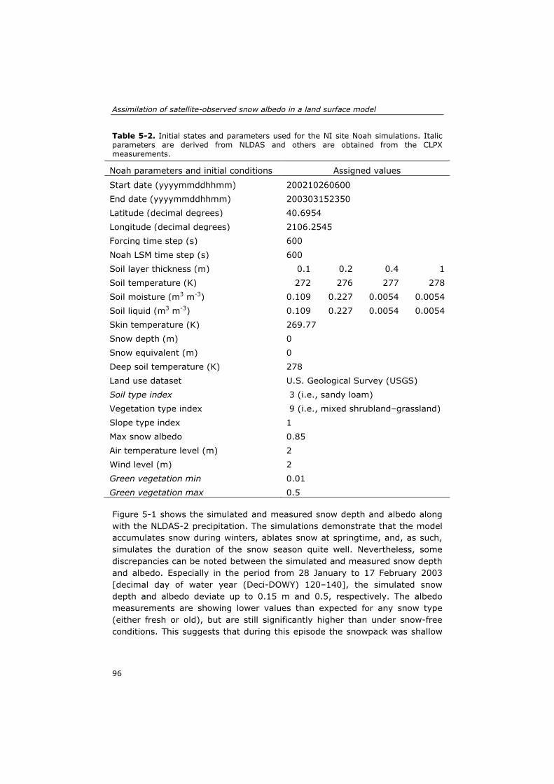
Assimilation of satellite-observed snow albedo in a land surface model
Table 5-2. Initial states and parameters used for the NI site Noah simulations. Italic parameters are derived from NLDAS and others are obtained from the CLPX measurements.
Noah parameters and initial conditions Assigned values
Start date (yyyymmddhhmm) 200210260600 End date (yyyymmddhhmm) 200303152350 Latitude (decimal degrees) 40.6954 Longitude (decimal degrees) 2106.2545 Forcing time step (s) 600 Noah LSM time step (s) 600 Soil layer thickness (m) 0.1 0.2 0.4 1 Soil temperature (K) 272 276 277 278 Soil moisture (m3 m-3) 0.109 0.227 0.0054 0.0054 Soil liquid (m3 m-3) 0.109 0.227 0.0054 0.0054 Skin temperature (K) 269.77 Snow depth (m) 0 Snow equivalent (m) 0 Deep soil temperature (K) 278 Land use dataset U.S. Geological Survey (USGS) Soil type index 3 (i.e., sandy loam) Vegetation type index 9 (i.e., mixed shrubland–grassland) Slope type index 1 Max snow albedo 0.85 Air temperature level (m) 2 Wind level (m) 2 Green vegetation min 0.01 Green vegetation max 0.5
Figure 5-1 shows the simulated and measured snow depth and albedo along with the NLDAS-2 precipitation. The simulations demonstrate that the model accumulates snow during winters, ablates snow at springtime, and, as such, simulates the duration of the snow season quite well. Nevertheless, some discrepancies can be noted between the simulated and measured snow depth and albedo. Especially in the period from 28 January to 17 February 2003 [decimal day of water year (Deci-DOWY) 120–140], the simulated snow depth and albedo deviate up to 0.15 m and 0.5, respectively. The albedo measurements are showing lower values than expected for any snow type (either fresh or old), but are still significantly higher than under snow-free conditions. This suggests that during this episode the snowpack was shallow
96
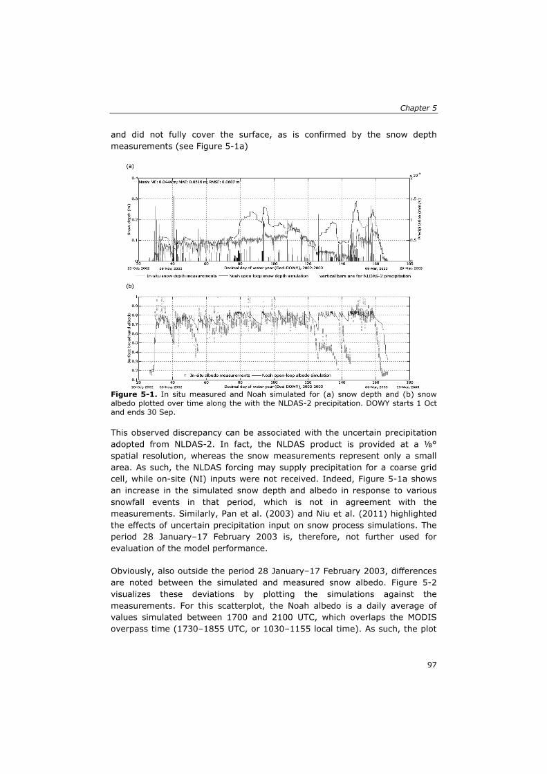
Chapter 5
and did not fully cover the surface, as is confirmed by the snow depth measurements (see Figure 5-1a)
Figure 5-1. In situ measured and Noah simulated for (a) snow depth and (b) snow albedo plotted over time along the with the NLDAS-2 precipitation. DOWY starts 1 Oct and ends 30 Sep.
This observed discrepancy can be associated with the uncertain precipitation adopted from NLDAS-2. In fact, the NLDAS product is provided at a ⅛° spatial resolution, whereas the snow measurements represent only a small area. As such, the NLDAS forcing may supply precipitation for a coarse grid cell, while on-site (NI) inputs were not received. Indeed, Figure 5-1a shows an increase in the simulated snow depth and albedo in response to various snowfall events in that period, which is not in agreement with the measurements. Similarly, Pan et al. (2003) and Niu et al. (2011) highlighted the effects of uncertain precipitation input on snow process simulations. The period 28 January–17 February 2003 is, therefore, not further used for evaluation of the model performance.
Obviously, also outside the period 28 January–17 February 2003, differences are noted between the simulated and measured snow albedo. Figure 5-2 visualizes these deviations by plotting the simulations against the measurements. For this scatterplot, the Noah albedo is a daily average of values simulated between 1700 and 2100 UTC, which overlaps the MODIS overpass time (1730–1855 UTC, or 1030–1155 local time). As such, the plot
97
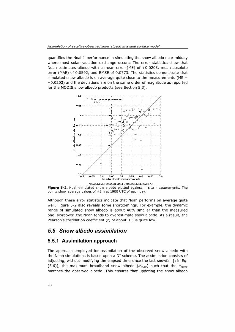
Assimilation of satellite-observed snow albedo in a land surface model
quantifies the Noah’s performance in simulating the snow albedo near midday where most solar radiation exchange occurs. The error statistics show that Noah estimates albedo with a mean error (ME) of +0.0203, mean absolute error (MAE) of 0.0592, and RMSE of 0.0773. The statistics demonstrate that simulated snow albedo is on average quite close to the measurements (ME = +0.0203) and the deviations are on the same order of magnitude as reported for the MODIS snow albedo products (see Section 5.3).
Figure 5-2. Noah-simulated snow albedo plotted against in situ measurements. The points show average values of ±2 h at 1900 UTC of each day.
Although these error statistics indicate that Noah performs on average quite well, Figure 5-2 also reveals some shortcomings. For example, the dynamic range of simulated snow albedo is about 40% smaller than the measured one. Moreover, the Noah tends to overestimate snow albedo. As a result, the Pearson’s correlation coefficient (r) of about 0.3 is quite low.
5.5 Snow albedo assimilation
5.5.1 Assimilation approach
The approach employed for assimilation of the observed snow albedo with the Noah simulations is based upon a DI scheme. The assimilation consists of adjusting, without modifying the elapsed time since the last snowfall [𝑡 in Eq. (5.6)], the maximum broadband snow albedo (𝛼𝑚𝑎𝑥) such that the 𝛼𝑠𝑛𝑜𝑤 matches the observed albedo. This ensures that updating the snow albedo
98
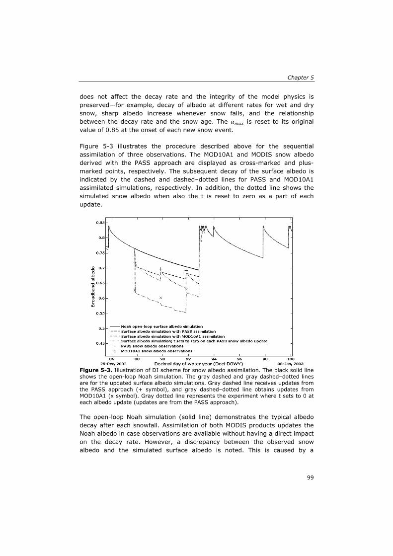
Chapter 5
does not affect the decay rate and the integrity of the model physics is preserved—for example, decay of albedo at different rates for wet and dry snow, sharp albedo increase whenever snow falls, and the relationship between the decay rate and the snow age. The 𝛼𝑚𝑎𝑥 is reset to its original value of 0.85 at the onset of each new snow event.
Figure 5-3 illustrates the procedure described above for the sequential assimilation of three observations. The MOD10A1 and MODIS snow albedo derived with the PASS approach are displayed as cross-marked and plus-marked points, respectively. The subsequent decay of the surface albedo is indicated by the dashed and dashed–dotted lines for PASS and MOD10A1 assimilated simulations, respectively. In addition, the dotted line shows the simulated snow albedo when also the t is reset to zero as a part of each update.
Figure 5-3. Illustration of DI scheme for snow albedo assimilation. The black solid line shows the open-loop Noah simulation. The gray dashed and gray dashed–dotted lines are for the updated surface albedo simulations. Gray dashed line receives updates from the PASS approach (+ symbol), and gray dashed–dotted line obtains updates from MOD10A1 (x symbol). Gray dotted line represents the experiment where t sets to 0 at each albedo update (updates are from the PASS approach).
The open-loop Noah simulation (solid line) demonstrates the typical albedo decay after each snowfall. Assimilation of both MODIS products updates the Noah albedo in case observations are available without having a direct impact on the decay rate. However, a discrepancy between the observed snow albedo and the simulated surface albedo is noted. This is caused by a
99
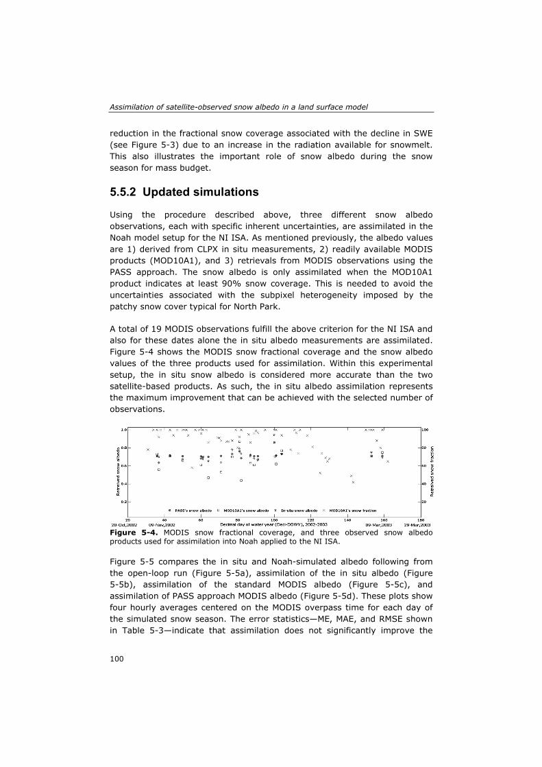
Assimilation of satellite-observed snow albedo in a land surface model
reduction in the fractional snow coverage associated with the decline in SWE (see Figure 5-3) due to an increase in the radiation available for snowmelt. This also illustrates the important role of snow albedo during the snow season for mass budget.
5.5.2 Updated simulations
Using the procedure described above, three different snow albedo observations, each with specific inherent uncertainties, are assimilated in the Noah model setup for the NI ISA. As mentioned previously, the albedo values are 1) derived from CLPX in situ measurements, 2) readily available MODIS products (MOD10A1), and 3) retrievals from MODIS observations using the PASS approach. The snow albedo is only assimilated when the MOD10A1 product indicates at least 90% snow coverage. This is needed to avoid the uncertainties associated with the subpixel heterogeneity imposed by the patchy snow cover typical for North Park.
A total of 19 MODIS observations fulfill the above criterion for the NI ISA and also for these dates alone the in situ albedo measurements are assimilated. Figure 5-4 shows the MODIS snow fractional coverage and the snow albedo values of the three products used for assimilation. Within this experimental setup, the in situ snow albedo is considered more accurate than the two satellite-based products. As such, the in situ albedo assimilation represents the maximum improvement that can be achieved with the selected number of observations.
Figure 5-4. MODIS snow fractional coverage, and three observed snow albedo products used for assimilation into Noah applied to the NI ISA.
Figure 5-5 compares the in situ and Noah-simulated albedo following from the open-loop run (Figure 5-5a), assimilation of the in situ albedo (Figure 5-5b), assimilation of the standard MODIS albedo (Figure 5-5c), and assimilation of PASS approach MODIS albedo (Figure 5-5d). These plots show four hourly averages centered on the MODIS overpass time for each day of the simulated snow season. The error statistics—ME, MAE, and RMSE shown in Table 5-3—indicate that assimilation does not significantly improve the
100
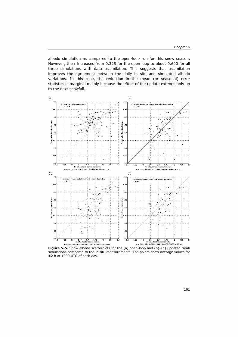
Chapter 5
albedo simulation as compared to the open-loop run for this snow season. However, the r increases from 0.325 for the open loop to about 0.600 for all three simulations with data assimilation. This suggests that assimilation improves the agreement between the daily in situ and simulated albedo variations. In this case, the reduction in the mean (or seasonal) error statistics is marginal mainly because the effect of the update extends only up to the next snowfall.
Figure 5-5. Snow albedo scatterplots for the (a) open-loop and (b)–(d) updated Noah simulations compared to the in situ measurements. The points show average values for ±2 h at 1900 UTC of each day.
101
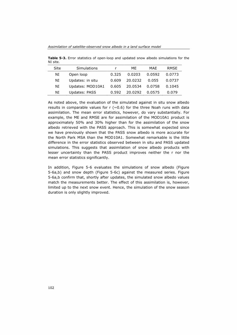
Assimilation of satellite-observed snow albedo in a land surface model
Table 5-3. Error statistics of open-loop and updated snow albedo simulations for the NI site.
Site Simulations r ME MAE RMSE
NI Open loop 0.325 0.0203 0.0592 0.0773 NI Updates: in situ 0.609 20.0232 0.055 0.0737 NI Updates: MOD10A1 0.605 20.0534 0.0758 0.1045 NI Updates: PASS 0.592 20.0292 0.0575 0.079
As noted above, the evaluation of the simulated against in situ snow albedo results in comparable values for r (~0.6) for the three Noah runs with data assimilation. The mean error statistics, however, do vary substantially. For example, the ME and RMSE are for assimilation of the MOD10A1 product is approximately 50% and 30% higher than for the assimilation of the snow albedo retrieved with the PASS approach. This is somewhat expected since we have previously shown that the PASS snow albedo is more accurate for the North Park MSA than the MOD10A1. Somewhat remarkable is the little difference in the error statistics observed between in situ and PASS updated simulations. This suggests that assimilation of snow albedo products with lesser uncertainty than the PASS product improves neither the r nor the mean error statistics significantly.
In addition, Figure 5-6 evaluates the simulations of snow albedo (Figure 5-6a,b) and snow depth (Figure 5-6c) against the measured series. Figure 5-6a,b confirm that, shortly after updates, the simulated snow albedo values match the measurements better. The effect of this assimilation is, however, limited up to the next snow event. Hence, the simulation of the snow season duration is only slightly improved.
102
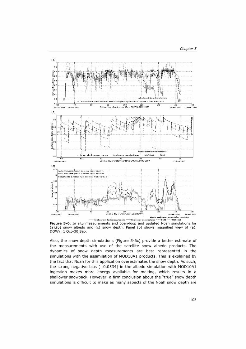
Chapter 5
Figure 5-6. In situ measurements and open-loop and updated Noah simulations for (a),(b) snow albedo and (c) snow depth. Panel (b) shows magnified view of (a). DOWY: 1 Oct–30 Sep.
Also, the snow depth simulations (Figure 5-6c) provide a better estimate of the measurements with use of the satellite snow albedo products. The dynamics of snow depth measurements are best represented in the simulations with the assimilation of MOD10A1 products. This is explained by the fact that Noah for this application overestimates the snow depth. As such, the strong negative bias (−0.0534) in the albedo simulation with MOD10A1 ingestion makes more energy available for melting, which results in a shallower snowpack. However, a firm conclusion about the “true” snow depth simulations is difficult to make as many aspects of the Noah snow depth are
103
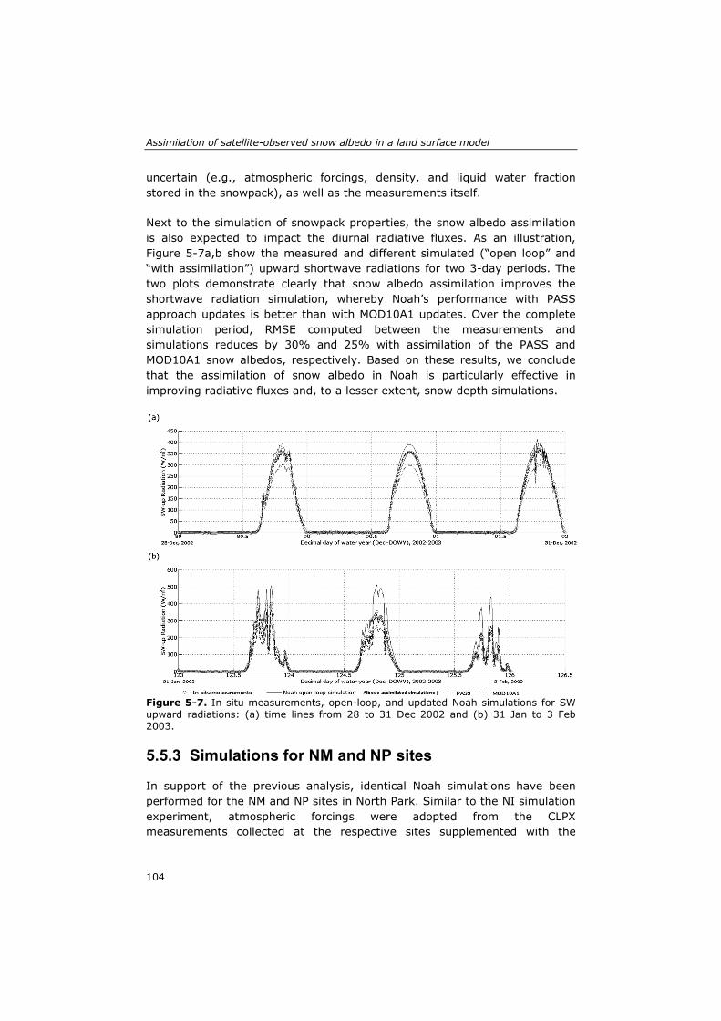
Assimilation of satellite-observed snow albedo in a land surface model
uncertain (e.g., atmospheric forcings, density, and liquid water fraction stored in the snowpack), as well as the measurements itself.
Next to the simulation of snowpack properties, the snow albedo assimilation is also expected to impact the diurnal radiative fluxes. As an illustration, Figure 5-7a,b show the measured and different simulated (“open loop” and “with assimilation”) upward shortwave radiations for two 3-day periods. The two plots demonstrate clearly that snow albedo assimilation improves the shortwave radiation simulation, whereby Noah’s performance with PASS approach updates is better than with MOD10A1 updates. Over the complete simulation period, RMSE computed between the measurements and simulations reduces by 30% and 25% with assimilation of the PASS and MOD10A1 snow albedos, respectively. Based on these results, we conclude that the assimilation of snow albedo in Noah is particularly effective in improving radiative fluxes and, to a lesser extent, snow depth simulations.
Figure 5-7. In situ measurements, open-loop, and updated Noah simulations for SW upward radiations: (a) time lines from 28 to 31 Dec 2002 and (b) 31 Jan to 3 Feb 2003.
5.5.3 Simulations for NM and NP sites
In support of the previous analysis, identical Noah simulations have been performed for the NM and NP sites in North Park. Similar to the NI simulation experiment, atmospheric forcings were adopted from the CLPX measurements collected at the respective sites supplemented with the
104
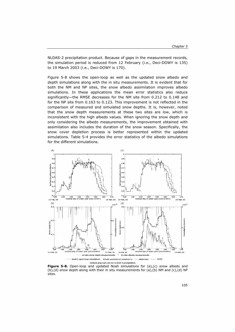
Chapter 5
NLDAS-2 precipitation product. Because of gaps in the measurement records, the simulation period is reduced from 12 February (i.e., Deci-DOWY is 135) to 19 March 2003 (i.e., Deci-DOWY is 170).
Figure 5-8 shows the open-loop as well as the updated snow albedo and depth simulations along with the in situ measurements. It is evident that for both the NM and NP sites, the snow albedo assimilation improves albedo simulations. In these applications the mean error statistics also reduce significantly—the RMSE decreases for the NM site from 0.212 to 0.148 and for the NP site from 0.163 to 0.123. This improvement is not reflected in the comparison of measured and simulated snow depths. It is, however, noted that the snow depth measurements at these two sites are low, which is inconsistent with the high albedo values. When ignoring the snow depth and only considering the albedo measurements, the improvement obtained with assimilation also includes the duration of the snow season. Specifically, the snow cover depletion process is better represented within the updated simulations. Table 5-4 provides the error statistics of the albedo simulations for the different simulations.
Figure 5-8. Open-loop and updated Noah simulations for (a),(c) snow albedo and (b),(d) snow depth along with their in situ measurements for (a),(b) NM and (c),(d) NP sites.
105
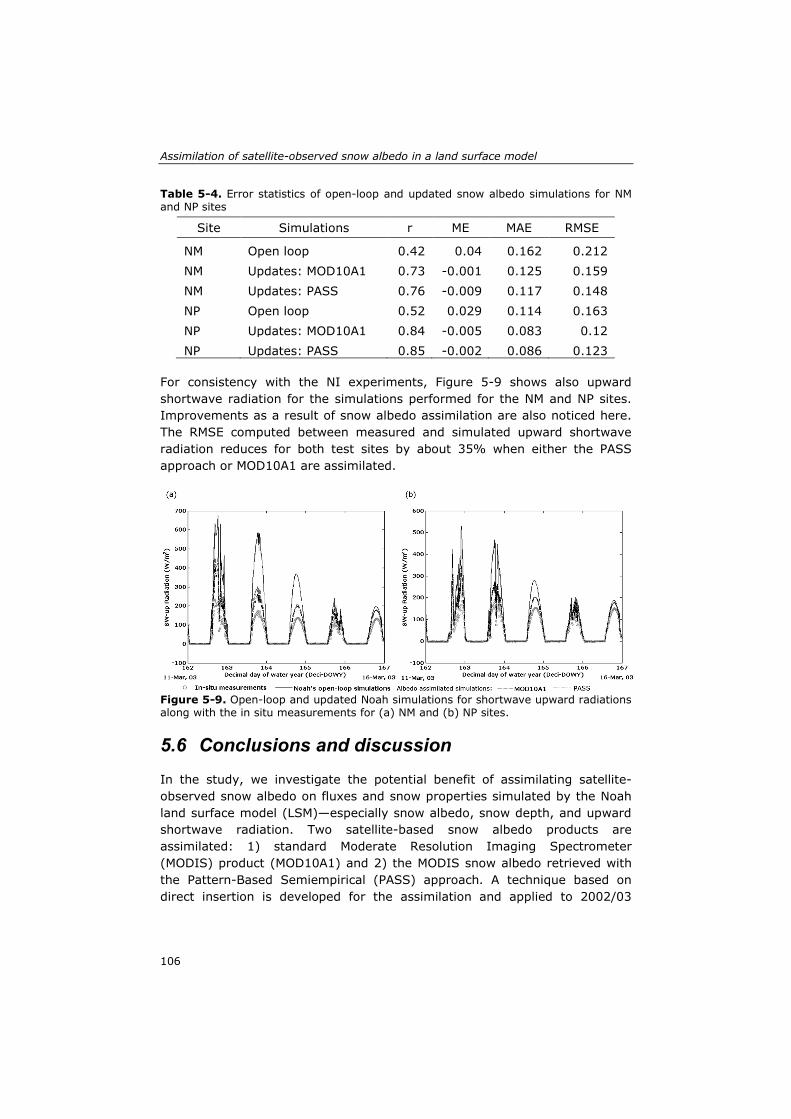
Assimilation of satellite-observed snow albedo in a land surface model
Table 5-4. Error statistics of open-loop and updated snow albedo simulations for NM and NP sites
Site Simulations r ME MAE RMSE
NM Open loop 0.42 0.04 0.162 0.212 NM Updates: MOD10A1 0.73 -0.001 0.125 0.159 NM Updates: PASS 0.76 -0.009 0.117 0.148 NP Open loop 0.52 0.029 0.114 0.163 NP Updates: MOD10A1 0.84 -0.005 0.083 0.12 NP Updates: PASS 0.85 -0.002 0.086 0.123
For consistency with the NI experiments, Figure 5-9 shows also upward shortwave radiation for the simulations performed for the NM and NP sites. Improvements as a result of snow albedo assimilation are also noticed here. The RMSE computed between measured and simulated upward shortwave radiation reduces for both test sites by about 35% when either the PASS approach or MOD10A1 are assimilated.
Figure 5-9. Open-loop and updated Noah simulations for shortwave upward radiations along with the in situ measurements for (a) NM and (b) NP sites.
5.6 Conclusions and discussion In the study, we investigate the potential benefit of assimilating satellite-observed snow albedo on fluxes and snow properties simulated by the Noah land surface model (LSM)—especially snow albedo, snow depth, and upward shortwave radiation. Two satellite-based snow albedo products are assimilated: 1) standard Moderate Resolution Imaging Spectrometer (MODIS) product (MOD10A1) and 2) the MODIS snow albedo retrieved with the Pattern-Based Semiempirical (PASS) approach. A technique based on direct insertion is developed for the assimilation and applied to 2002/03
106
Chapter 5
North Park snow season observed at three sites during the Cold Land Process Field Experiment (CLPX).
The comparison with in situ measurements shows that, in general, assimilation improves the snow albedo simulations. A reduction in the mean (or seasonal) error statistics is, however, not evident for all three CLPX sites. This is attributed to the limited impact of snow albedo updates beyond the following snow event. Analyses also suggest that simulation of snow depth and the duration of snow season tend to improve with snow albedo assimilation. However, a firm conclusion on this aspect is not possible because of the many uncertainties involved in the modeling as well as measurement of these processes. The most noticeable improvements obtained with assimilation are in the simulation of the upward shortwave radiation. With both satellite-based albedo products the root-mean-square errors decrease by about 30%.
Therefore, we conclude that the assimilation of the satellite-observed snow albedo ameliorates the simulation of upward shortwave radiation during the snow season, which is a prerequisite for an improved simulation of both the surface energy budget and the snowpack properties. These promising effects of snow albedo assimilation can help to reduce the uncertainties in the medium-range weather forecast as well as prediction of hydrological process (e.g., runoff). Further amelioration of the snow mass simulation is only possible with accurate knowledge of snow depth and/or water equivalent collected either via in situ measurement or from space. The data products that are expected to evolve from Earth Explorer missions of the European Space Agency (e.g., Cold Regions H2O) and NASA (e.g., Snow and Cold Land Processes) can play an important role in this context.
107

Assimilation of satellite-observed snow albedo in a land surface model
108
6 Thesis’ conclusions Snow cover dynamics affect the fresh water supply, weather and climate at regional as well as global scales. Snow coverage, water equivalent, and albedo are the snowpack variables that directly affect the energy and water budgets of the land surface. The research described in this thesis focuses on improving the simulation of snow processes and thus the water and heat exchanges at the snow-covered land-atmosphere interface. This is expected to improve climate and hydrologic simulations.
Land Surface Models (LSMs) represent the land processes within Numerical Weather Prediction models and typically accommodate the snow processes, enabling the quantification of the fluxes under snow covered conditions. The reliability of the simulations is, however, determined by the model initialization, structure, parameterization, and atmospheric forcings. As such, the reliability of the LSM simulations may improve through the amelioration of each of the model components. The research described in this thesis contribute to the improvement of LSM simulations by investigating i) advanced methods of model initialization (e.g., assimilation of satellite observation), and ii) modification to the model parameterization.
The structure of this thesis is as follows. Chapter 2 introduces a Pattern based Semi-empirical (PASS) approach that account for imaging geometry effects while retrieving snow albedo estimates from satellite observations, and Chapter 3 describes retrieval of fraction snow coverage from dual-view satellite observations under different atmospheric visibility conditions. Chapter 4 introduces a snow albedo parameterization for LSMs and quantifies impact of different snow albedo parameterizations on the simulations of surface energy and water budgets. Chapter 5 describes satellite-retrieved snow albedo assimilation in the Noah LSM. Each of these is summarized below to answer the thesis’ research questions.
6.1 Satellite observation of snow properties Snow albedo is a variable primarily sensitive to snow grains and used in modeling to partition solar radiative flux at the snow-atmosphere interface. Snow is more absorptive and a more anisotropic reflector in the near-infrared region of the solar spectrum than in the visible region. Thus, the near-infrared albedo plays an important role in the energy-mass balance of a snow surface and challenges the retrieval from remote sensing (RS) because satellite sensors only measure reflectance in certain sun-sensor configurations.
109
Thesis’ conclusions
Chapter 2 presents a PAttern-baSed Semi-empirical (PASS) approach that quantifies spectral reflectance patterns formed at 1.240 µm wavelength due to varying sun-sensor geometry for a range of snow grain sizes to account for the anisotropy in the near-infrared region. Geometrically, these patterns are characterized by right-triangle whose base and height are functions of solar zenith and scattering angles, respectively and centroid is in direct relation with the spectral albedo at 1.240 µm. The semi-empirical relationship is then used to retrieve near-infrared albedo, which is integrated with the visible albedo using the parameterization from the Snow THERmal Model (SNTHERM) for the estimation of the broadband snow albedo.
The approach shows better accuracy for spectral albedo estimates than for those computed using the Lambertian reflectance assumption for snow, reducing the error in the range and standard deviation by 75% and 65%, respectively. Applying the approach to MODIS-measured radiances (i.e, MOD02HKM MODIS product), the retrieved albedo – with a mean error of 0.002 on a seasonal scale – is found to be in good agreement (r=0.82) with in situ measurements from prairie sites and is almost 50% better than the daily MODIS snow albedo product (i.e., MOD10A1). Further studies are needed to establish the validity of the approach for different types of snow (e.g., alpine, tundra) on different land covers and topography.
Chapter 3 presents a concept to correct retrieved fraction snow coverage (FSC) for atmospheric effects from dual-view coarse-scale RS. Snow, as discussed in Chapter 2, is highly anisotropic and less reflecting medium in the near-infrared region, whereas highly reflective and less anisotropic in the visible region. Further, the reflectance in visible region is also less sensitive to snow age (snow grains) than in the near-infrared region of the solar spectrum and provides high contrast with bare ground. Therefore, the method uses visible band to retrieve snow coverage and dual-views to correct the estimates for the atmospheric aerosols effects.
DIScrete Ordinates Radiative Transfer (DISORT) coupled to MODerate resolution atmospheric TRANsmission (MODTRAN) simulations suggest that fractional snow coverage estimates retrieved using linear unmixing of top-of-atmosphere RS measurements in the visible region can be corrected for by measuring the relative contrast difference between the nadir and inclined views. However, the relative contrast between the views depends, besides atmospheric visibility, also on solar zenith angle and surface altitude. The method presented in the Chapter 3 accounts for the solar zenith angle effect on the relative contrast measurements for low altitude snow-covered land surface.
110
Chapter 6
Theoretically, the method can retrieve FSC at pixel scale from nadir view with an uncertainty of about ± 2.5%, which is almost tenfold better than the theoretical uncertainty of widely used NDSI based FSC estimates. However, there are some concerns that need to be addressed in the future for the development of a real operational algorithm for FSC mapping from dual-view RS observations – especially, the effects of surface altitude and relative azimuth angle between the sun and sensor, which changes atmospheric radiance contribution to total measured radiance at the sensor by changing the atmospheric path length: the distance that electromagnetic energy must traverse through the earth's atmosphere.
6.2 Land surface modeling The Earth’s weather, climate, and hydrological systems are complex, interactive systems consisting of the atmosphere, land surface, and oceans. Land surface models (LSMs) in this regard simulate the interaction between the land surface and atmosphere using various parameterizations for different land surface processes. Almost all LSMs use empirical parameterizations to simulate snowpack processes including the snow albedo evolution.
Chapter 4 presents characterization of the in situ measured snow albedo evolution during melting of alpine, prairie, and tundra snowpacks. The measurements of alpine snowpacks show that albedo drops to the minimum value of snow albedo at a rate, stays at the value till the snowpack remains optically thick, and starts to drop further under the influence of background albedo when the melting snowpack (also prairie and tundra snowpacks) becomes optically thin.
The Noah LSM offline point-scale simulations of snow albedo with the existing parameterizations (i.e., Noah’s default, BATS, and CLASS LSMs’ parameterizations) reveal that the parameterizations lack explicit characterization of the observed snow albedo evolution features. This results in an overestimation of the snow albedo during springtime, which contributes to a prolonged simulated existence of the snowpack by reducing the ablation rate.
As far as the alpine snowpack remains optically thick, the observed features of albedo evolution suggest variogram type models with range and sill can explicitly characterize the evolution. The range parameter controls the evolution rate by defining the time since the onset of melting needed for an alpine snowpack to reach the minimum snow albedo value, i.e., sill. From the instant when the snowpack becomes optically thin, the further decline in albedo is, however, simulated by mixing the snow and the background
111
Thesis’ conclusions
albedos as a weighted function of snow depth. This piecewise parameterization is referred to as the variogram-shaped (VAS) parameterization.
The implementation of the VAS parameterization in the Noah LSM improves the snow albedo simulation of the alpine and tundra snowpacks by almost 25% (in terms of RMSE) over the existing parameterizations. Consequently, the simulated snow depth, snowmelt, and upward shortwave radiation are improved on-average by about 20%, 15%, and 30%, respectively. However, further studies are needed to draw firm conclusions for the prairie type snowpacks.
The improvements obtained at point-scale with the VAS parameterization consist essentially of a lower deep snowpack albedo for the melt season that accelerates the melt rate and associated surface hydrological processes. Hence, Noah at large-scale with the VAS parameterization simulates more evapotranspiration and larger runoff peaks in Spring whereas the Summer runoff is lower than simulated with the default snow albedo parameterization.
6.3 Use of observations for modeling Although Chapter 4 presents a better parameterization to simulate snow albedo evolution during springtime, uncertainties in albedo simulation are still noted during both winter and springtimes. The uncertainties in the snow albedo simulation arise mainly from the fact that snow albedo evolution is a function of atmospheric forcings but parameterized using empirical relationships between snow age (i.e, time elapsed since last snowfall and onset of melting during accumulation and ablation, respectively) and albedo. These relationships, independent of atmospheric dynamics, decrease snow albedo as snow age progresses.
Earth observations are sensitive to the land surface state and are used to retrieve snow albedo in Chapter 2. The retrieved snow albedo from the observations represents the state of snow albedo owing to the history of atmospheric dynamics near the snow surface, which models approximate as a function of snowpack's age. Improvement in snow albedo simulation is, therefore, expected via integration of the retrieved snow albedo with the model simulation of snow albedo. Data assimilation, in this regard, provides a framework for utilizing information from observations for reducing uncertainties in model simulations and make them consistent with observations.
As discussed, the LSM's parameterizations for snow albedo use snow age to model snow albedo evolution (Chapter 4). This makes the relationship
112
Chapter 6
between the snow age and decay rate important. Therefore, the presented snow albedo assimilation approach consists of adjusting, without modifying the elapsed time since the last snowfall or snowmelt onset, the simulated maximum broadband snow albedo such that it matches the observed albedo. Because the approach preserves the elapsed time since the last snowfall or snowmelt onset, it can be implemented with all the four albedo parameterizations discussed in Chapter 4.
The presented approach directly ingests the observations by assuming the observations are accurate. This is, however, rare in case if retrievals from RS are used. Therefore, the impact of this assumption is quantified using three different snow albedo observations, each with specific inherent uncertainties: in situ albedo observations (considered highly accurate), retrievals from RS using two different algorithms (i.e., MODIS daily standard snow albedo product and PASS algorithm presented in Chapter 2).
In Chapter 5, the assimilation approach is tested with Noah’s default snow albedo parameterization for the prairie snowpacks. The results demonstrate the assimilation of snow albedo observations improves the agreement between the simulated and measured daily snow albedo. However, the improvement of the simulation at seasonal scale may be marginal depending on the frequency of the snowfall events because the effect of the assimilation extends only up to the next snow event. Further, the snow albedo simulation improves the most with the assimilation of in situ observed snow albedo – the highly reliable estimates of snow albedo. The assimilation of the in situ observations increased the correlation (r) between the measured and simulated snow albedo by about 90% over the non-assimilated simulation. However, the assimilation of MODIS- and PASS- retrieved snow albedo estimates improves the r respectively by 72% and 76%. Therefore, high frequency of snowfall events (by shortening the memory of assimilation) and low reliability of assimilated inputs (by misguiding the model) limit the efficiency of the snow albedo assimilated simulations.
As in Chapter 4, improvements in snow albedo simulation – here obtained via assimilation of observed snow albedo estimates – improves the simulation of snow depth, duration for the snow season, and improves the most upward shortwave radiation simulation. The RMSE between the measured and simulated upward shortwave radiation reduces by about 30% with the assimilation of either satellite-based albedo product over the non-assimilated simulation. Further amelioration of the simulation of snowpack properties is only possible with accurate knowledge of snow depth and/or water equivalent (a component of water mass balance) collected either via in situ measurement or from space. Data products that are expected to evolve from Earth Explorer missions of the European Space Agency (e.g., Cold Regions
113

Thesis’ conclusions
H2O) and NASA (e.g., Snow and Cold Land Processes) can play an important role in this context.
6.4 Limitations and recommendations Although the thesis demonstrates improvements in the fluxes’ simulation at the snow covered land-atmosphere interface via the improved snowpack’s representation in a LSM, it has some limitations. Interesting avenues for future research are highlighted below.
1. The model presented in Chapter 2 for retrieving broadband albedo of snow from RS is primarily based on near-infrared albedo and validated for the sites having low-lying grass/shrubs on flat topography. Therefore, further enhancements could be achieved via the explicit handling of:
I. visible albedo, which is sensitive to impurities at snow surface and atmospheric aerosols;
II. sub-scale/sub-pixel topographic variations, which would extend its applicability to topographically complex snow-covered regions of the globe;
III. forest cover, which allow to retrieve snow albedo under sparse forest canopies.
2. The concept presented in Chapter 3 for fractional snow cover mapping – yet to be validated – corrects the retrieved coverage estimates for the atmospheric effects using the relative contrast difference between the two views (nadir and inclined). To make it a real operational algorithm for FSC mapping,
I. MODTRAN simulations are needed for different surface altitudes and relative azimuth angles between the sun and sensor to parameterize the approach with different set of coefficients.
II. uncertainties need to be quantified – due to the assumption of Lambertian reflection in the visible region at course spatial scale for the snow – using the coupled simulations of DISORT and MODTRAN radiative transfer models.
3. The assessment of the parameterization presented in Chapter 4 for snow albedo evolution highlights:
I. Besides the overall energy balance at the snowpack’s surface, the snowpack’s density parameterization needs to be intensively studied.
II. The prairie snowpacks, which are the most dynamic snowpacks, needs to be thoroughly studied.
4. Chapter 5 concludes that assimilation of observed snow albedo ameliorates the simulations of upward shortwave radiations. Further amelioration, even in the simulation of snow mass, is only possible (keeping in view the limitations of Chapter 4) with the assimilation of
114
Chapter 6
SWE – either observed via in situ sensors or from satellite remote sensing.
6.5 Final remarks Snow constantly metamorphoses throughout its existence on the land surface at rates depending on the near-surface atmospheric dynamics. The physical properties of snow, including snow grains shape and size, change due to the metamorphic processes. Snow grains grow over time due to vapor deposition and melting-refreezing of the snowpack; the growth decreases snow albedo. The decreasing snow albedo absorbs more incoming solar radiation that warms the snow and thus accelerates metamorphic processes – including ablation that affects magnitude and timings of streamflow peaks, land surface states, and also the strength of snow albedo feedback (SAF), which affects global annual mean surface air temperature: a variable often used to measure climate sensitivity.
The Fourth and Fifth Assessment Reports by the Intergovernmental Panel on Climate Change show large intermodel spread in SAF strength (IPCC 2007, 2013). The spread is mostly attributed to a large spread in effective snow albedo (includes canopy effects on snow albedo; Qu & Hall 2007). The thesis presents novel approaches to retrieve snow albedo from RS data, parameterize snow albedo in LSM, and assimilate the retrievals in the LSM simulations, which ultimately improve snow albedo simulations and thus impact positively the energy and water fluxes' simulations at the snow-covered land surface. Therefore, the outcomes of the thesis are likely to be useful in constraining the snow albedo parameterizations and thus reducing the SAF spread in the next generation climate models.
Further, the streamflows in snowmelt-dominated* (e.g., Colorado river basin, U.S.; Churchill river basin, U.S.; Angara River, Russia) and snowmelt-dependent** (e.g., Indus river basin, Pakistan) basins are sensitive to the snow properties (e.g., snow water equivalent, snow albedo, snow coverage) that determine the energy and mass (snow) available for melt at the land surface. In basins where inhabitants' livelihood and country's economy (socio, micro, and macro) - such as the Indus basin – depend primarily on the snow/glacier melt, the observations and simulations of snow cover properties (e.g., snow albedo, water equivalent, coverage, detection of snowmelt onset) become imperative for well-informed water resource ________________ * Snowmelt-dominated basin: the ratio of the accumulated annual snowfall to annual runoff > 0.5. ** Snowmelt-dependent basin: water availability is predominantly influenced by snowmelt generated upstream.
115

Thesis’ conclusions
management. In this context, the studies on improving the understanding of snow processes and measurement techniques – such as this thesis – can contribute in various socio-economic developmental plans via improving the land surface states and seasonal streamflow predictions.
Although the approaches presented in this thesis are validated and improvements are shown at limited spatial and temporal scales, it is expected that these approaches will be effective at regional and global scales to improve simulation of the fluxes at the land-atmosphere interface and thus contribute positively the socio-economic developments. However, follow-on studies should be undertaken to verify the approaches at different spatial scales and physiographic conditions.
116
Bibliography Allen, R.J., & Zender, C.S. (2010). Effects of continental-scale snow albedo
anomalies on the wintertime Arctic oscillation. Journal of Geophysical Research, 115(D23), D23105.
Anderson, E.A. (1973). National weather service river forecast system-snow accumulation and ablation model. NOAA Technical Memorandum NWS HYDRO-17.
Anderson, E.A. (1976). A Point Energy and Mass Balance Model of a Snow Cover. Office of Hydrology, National Weather Service, 150.
Andreadis, K.M. & Lettenmaier, D.P. (2006). Assimilating remotely sensed snow observations into a macroscale hydrology model. Advances in Water Resources, 29(6), 872-886.
Aoki, T., Hori, M., Motoyoshi, H., Tanikawa, T., Hachikubo, A., Sugiura, K., Yasunari, T.J., Storvold, R., Eide, H.A., Stamnes, K., Li, W., Nieke, J., Nakajima, Y., & Takahashi, F. (2007). ADEOS-II/GLI snow/ice products — Part II: Validation results using GLI and MODIS data. Remote Sensing of Environment, 111, 274-290.
Arsenault, K. R., P. R. Houser, & G. J. M. De Lannoy (2014), Evaluation of the MODIS snow cover fraction product, Hydrological Processes, 28(3), 980-998.
Arsenault, K. R., P. R. Houser, G. J. M. De Lannoy, & P. A. Dirmeyer (2013), Impacts of snow cover fraction data assimilation on modeled energy and moisture budgets, Journal of Geophysical Research: Atmospheres, 118(14), 7489-7504.
Barlage, M., Chen, F., Tewari, M., Ikeda, K., Gochis, D., Dudhia, J., Rasmussen, R., Livneh, B., Ek, M., & Mitchell, K. (2010). Noah land surface model modifications to improve snowpack prediction in the Colorado Rocky Mountains. Journal of Geophysical Research, 115(D22), D22101.
Barnett, T. P., Adam, J. C., & Lettenmaier, D. P. (2005). Potential impacts of a warming climate on water availability in snow-dominated regions. Nature, 438(7066), 303–309.
Berk, A., G. P. Anderson, P. K. Acharya, J. H. Chetwynd, M. L. Hoke, L. S. Bernstein, E. P. Shettle, M. W. Matthew, & S. M. Adler-Golden (1999), MODTRAN4 version 2 user's manual, Air Force Research Laboratory, Space Vehicles Directorate, Hanscom AFB, MA, USA.
Biancamaria, S., Mognard, N.M., Boone, A., Grippa, M., & Josberger, E.G. (2008). A satellite snow depth multi-year average derived from SSM/I for the high latitude regions. Remote Sensing of Environment, 112, 2557-2568.
Bourgeois, C.S., Calanca, P., & Ohmura, A. (2006). A field study of the hemispherical directional reflectance factor and spectral albedo of dry snow. Journal of Geophysical Research, 111(D20), D20108.
117
Bibliography
Broyden, C.G. (1970). The Convergence of a Class of Double-rank Minimization Algorithms 1. General Considerations. IMA Journal of Applied Mathematics, 6, 76-90.
Chen, D., Huang, J., & Jackson, T.J. (2005). Vegetation water content estimation for corn and soybeans using spectral indices derived from MODIS near- and short-wave infrared bands. Remote Sensing of Environment, 98(2-3), 225-236.
Cherkauer, K.A., Bowling, L.C., & Lettenmaier, D.P. (2003). Variable infiltration capacity cold land process model updates. Global and Planetary Change, 38(1-2), 151-159.
Christensen, N. S., & D. P. Lettenmaier (2007), A multimodel ensemble approach to assessment of climate change impacts on the hydrology and water resources of the Colorado River Basin, Hydrology and Earth System Sciences, 11(4), 1417-1434.
Cline, D.W. (1997a). Effect of seasonality of snow accumulation and melt on snow surface energy exchanges at a continental Alpine site. Journal of Applied Meteorology, 36(1), 32-51.
Cline, D.W. (1997b). Snow surface energy exchanges and snowmelt at a continental, midlatitude Alpine site. Water Resources Research, 33(4), 689-701.
Colbeck, S.C. (1975). A theory for water flow through a layered snowpack. Water Resources Research, 11, 261-266.
Colbeck, S.C. (1982). An overview of seasonal snow metamorphism. Reviews of Geophysics, 20, 45-61.
Colbeck, S.C. (1983). Theory of metamorphism of dry snow. Journal of Geophysical Research, 88(C09), 5475-5482.
Conway, H., & Benedict, R. (1994). Infiltration of water into snow. Water Resources Research, 30, 641-649.
Davis, R., 2003. Land Processes Distributed Active Archive Center. CLPX-Satellite: Landsat Thematic Mapper Imagery Compiled by R. Davis of CRREL. Boulder, CO: National Snow and Ice Data Center. Digital Media.
Dente, L., Satalino, G., Mattia, F., & Rinaldi, M. (2008). Assimilation of leaf area index derived from ASAR and MERIS data into CERES-Wheat model to map wheat yield. Remote Sensing of Environment, 112(4), 1395–1407.
DeWalle, D. R. & Rango, A. (2008). Principles of Snow Hydrology. Cambridge University Press, 420 pp.
Dickinson, R.E., Henderson-Sellers, A., & Kennedy, P.J. (1993). Biosphere-Atmosphere Transfer Scheme (BATS) version 1e as coupled to the NCAR Community Climate Model. NCAR Technical Note NCAR/TN-387+STR; National Center for Atmospheric Research, Boulder, CO.
Dobreva, I., & Klein, A. (2011). Fractional snow cover mapping through artificial neural network analysis of MODIS surface reflectance. Remote Sensing of Environment, 115, 3355-3366.
118
Bibliography
Dozier, J., & Painter, T. (2004). Multispectral and hyperspectral remote sensing of alpine snow properties. Annual Review of Earth and Planetary Sciences, 32, 465-494.
Dozier, J., Green, R. O., Nolin, A. W., & Painter, T. H. (2009). Interpretation of snow properties from imaging spectrometry. Remote Sensing of Environment, 113 (Supplement 1), S25–S37.
Ek, M.B., Mitchell, K.E., Lin, Y., Rogers, E., Grunmann, P., Koren, V., Gayno, G., & Tarpley, J.D. (2003). Implementation of Noah land surface model advances in the National Centers for Environmental Prediction operational mesoscale Eta model. Journal of Geophysical Research, 108(D22), 8851.
Ek, M.B., Xia, Y., Wood , E., Sheffield, J., Luo , L., Lettenmaier , D., Livneh , B., Mocko, D., Cosgrove , B., Meng, J., Wei, H., Koren, V., Schaake , J., Mo, K., Fan , Y., Duan , Q., & Mitchell, K. (2011). North American Land Data Assimilation System Phase 2 (NLDAS-2): Development and applications. GEWEX News, No. 21, International GEWEX Project Office, Silver Spring, MD, 6–7.
Elder, K., & Goodbody, A. (2004). CLPX-Ground: ISA Main Meteorological Data. Boulder, CO, USA: National Snow and Ice Data Center. [Available online at http://nsidc.org/data/docs/daac/nsidc0172_clpx_mainmet/, accessed 4 December 2013].
Elder, K., Goodbody, A., Cline, D., Houser, P., Liston, G. E., Mahrt, L., & Rutter, N. (2009). NASA Cold Land Processes Experiment (CLPX 2002/03): Ground-based and near-surface meteorological observations. Journal of Hydrometeorology, 10(1), 330–337.
ESA (2009). Candidate Earth Exploreer CoRe Mission: CoReH2O. Report for Assessment. ESA SP-1313/3. ESA, Noordwijk, NL.
ESA (2012). Report for Mission Selection: CoReH2O. ESA SP1334/2 (3 volume series). ESA, Noordwijk, NL.
Faurtyot, T. & Baret, F., 1997. Vegetation water and dry matter contents estimated from top-of-the-atmosphere reflectance data: A simulation study. Remote Sensing of Environment, 61(1), 34-45.
Feng, X., Sahoo, A., Arsenault, K., Houser, P., Luo, Y., & Troy, T. J. (2008). The impact of snow model complexity at three CLPX sites. Journal of Hydrometeorology, 9(6), 1464–1481.
Fletcher, C.G., Hardiman, S.C., Kushner, P.J., & Cohen, J. (2009a). The Dynamical Response to Snow Cover Perturbations in a Large Ensemble of Atmospheric GCM Integrations. Journal of Climate, 22(5), 1208-1222.
Fletcher, C.G., Kushner, P.J., Hall, A., & Qu, X. (2009b). Circulation responses to snow albedo feedback in climate change. Geophysical Research Letters, 36(9), L09702.
Fletcher, R. (1970). A new approach to variable metric algorithms. The Computer Journal, 13, 317-322.
119
Bibliography
Foster, J.L., Chang, A.T.C., & Hall, D.K. (1997). Comparison of snow mass estimates from a prototype passive microwave snow algorithm, a revised algorithm and a snow depth climatology. Remote Sensing of Environment, 62, 132-142.
Franz, K. J., & L. R. Karsten (2013), Calibration of a distributed snow model using MODIS snow covered area data, Journal of Hydrology, 494(0), 160-175.
Frei, A., & Robinson, D.A. (1999). Northern Hemisphere snow extent regional variability 1972-1994. International Journal of Climatology, 19, 1535-1560.
Goldfarb, D. (1970). A Family of Variable-Metric Methods Derived by Variational Means. Mathematics of Computation, 24, 23-26.
Green, R. O., Dozier, J., Roberts, D., & Painter, T. (2002). Spectral snow-reflectance models for grain-size and liquid–water fraction in melting snow for the solar reflected spectrum. Annals of Glaciology, 34, 71–73.
Hachikubo, A., & Akitaya, E. (1997). Effect of wind on surface hoar growth on snow. Journal of Geophysical Research, 102(D04), 4367-4373.
Hall, D. K., G. A. Riggs, & V. V. Salomonson (2006), MODIS/Terra Snow Cover 8-day L3 Global 500m Grid V005 (MODIS Snow Products User Guide to Collection 5), Boulder, Colorado USA: National Snow and Ice Data Center.
Hall, D.K., Riggs, G.A., & Salomonson, V.V. (1995). Development of methods for mapping global snow cover using moderate resolution imaging spectroradiometer data. Remote Sensing of Environment, 54, 127-140.
Hallikainen, M.T., & Jolma, P.A. (1992). Comparison of algorithms for retrieval of snow water equivalent from Nimbus-7 SMMR data in Finland. Geoscience and Remote Sensing, IEEE Transactions on, 30, 124-131.
Hori, M., Aoki, T., Stamnes, K., & Li, W. (2007). ADEOS-II/GLI snow/ice products — Part III: Retrieved results. Remote Sensing of Environment, 111, 291-336.
Immerzeel, W.W., van Beek, L.P.H. & Bierkens, M.F.P. (2010). Climate Change Will Affect the Asian Water Towers. Science, 328(5984), 1382-1385.
IPCC (2007). Fourth Assessment Report on Climate Change: The Physical Science Basis (Chapter 8: Climate Models and Their Evaluation). Cambridge, United Kingdom and New York, USA: Cambridge University Press.
IPCC (2013). Fifth Assessment Report on Climate Change: The Physical Science Basis (Chapter 9. Evaluation of Climate Models). Cambridge, United Kingdom and New York, USA: Cambridge University Press.
Jin, J., & Miller, N. (2007). Analysis of the impact of snow on daily weather variability in mountainous regions using MM5. Journal of Hydrometeorology, 8, 245-258.
120
Bibliography
Jin, J., Gao, X., Yang, Z., Bales, R., Sorooshian, S., & Dickinson, R. (1999). Comparative analyses of physically based snowmelt models for climate simulations. Journal of Climate, 12, 2643-2657.
Jordan, P. (1983a). Meltwater movement in a deep snowpack 1. Field observations. Water Resources Research, 19, 971-978.
Jordan, P. (1983b). Meltwater movement in a deep snowpack 2. Simulation model. Water Resources Research, 19, 979-985.
Jordan, R. (1991). A one-dimensional temperature model for a snow cover: Technical documentation for SNTHERM.89, Special Report 91–16. Hanover, NH: U.S. Army Cold Regions Research and Engineering Laboratory.
Josberger, E., & Mognard, N. (2002). A passive microwave snow depth algorithm with a proxy for snow metamorphism. Hydrological Processes, 16, 1557-1568.
Kaufman, Y.J., Kleidman, R.G., Hall, D.K., Martins, J.V. & Barton, J.S. (2002). Remote sensing of subpixel snow cover using 0.66 and 2.1 μm channels. Geophysical Research Letters, 29(16), 1781.
Kelly, R.E., Chang, A.T., Leung, T., & Foster, J.L. (2003). A prototype AMSR-E global snow area and snow depth algorithm. Geoscience and Remote Sensing, IEEE Transactions on, 41, 230-242.
Klein, A. G., & Stroeve, J. (2002). Development and validation of a snow albedo algorithm for the MODIS instrument. Annals of Glaciology, 34, 45–52.
Koivusalo, H., & Heikinheimo, H. (1999). Surface energy exchange over a boreal snowpack: comparison of two snow energy balance models. Hydrological Processes, 13, 2395-2408
Kokhanovsky, A. A. & Zege , E. P. (2004). Scattering optics of snow. Applied Optics, 43 (7), 1589–1602.
Koren, V., Schaake, J., Mitchell, K., Duan, Q.Y., Chen, F., & Baker, J.M. (1999). A parameterization of snowpack and frozen ground intended for NCEP weather and climate models. Journal of Geophysical Research, 104(D16), 19569-19585.
Levy, R.C., Remer, L.A. & Dubovik, O., 2007. Global aerosol optical properties and application to Moderate Resolution Imaging Spectroradiometer aerosol retrieval over land. Journal of Geophysical Research, 112(D13), D13210.
Li, W., Stamnes, K., Eide, H., & Spurr, R. (2007). Bidirectional reflectance distribution function of snow: Corrections for the Lambertian assumption in remote sensing applications. Optical Engineering, 46(6), 066201-1–066201-9.
Liang, S. (2004). Quantitative remote sensing of land surfaces. New York: John Wiley & Sons, Inc. Chapter 4.
Liang, S., Stroeve, J., & Box, J. E. (2005). Mapping daily snow/ice shortwave broadband albedo from Moderate Resolution Imaging Spectroradiometer
121
Bibliography
(MODIS): The improved direct retrieval algorithm and validation with Greenland in situ measurement. Journal of Geophysical Research, 110(D10), D10109.
Liu, Y., C. D. Peters-Lidard, S. Kumar, J. L. Foster, M. Shaw, Y. Tian, & G. M. Fall (2013), Assimilating satellite-based snow depth and snow cover products for improving snow predictions in Alaska, Advances in Water Resources, 54(0), 208-227.
Livneh, B., Xia, Y.L., Mitchell, K.E., Ek, M.B., & Lettenmaier, D.P. (2010). Noah LSM Snow Model Diagnostics and Enhancements. Journal of Hydrometeorology, 11(3), 721-738.
Luojus, K., Pulliainen, J., Takala, M., Lemmetyinen, J., Derksen, C., & Wang, L. (2010). Global snow monitoring for climate research, SnowWater Equivalent (SWE) product guide In: European Space Agency Study Contract Report ESRIN Contract 21703/08/I-EC. available at: www.globsnow.info/swe/GlobSnow_SWE_product_readme_v1.0a.pdf
Lyapustin, A., Tedesco, M., Wang, Y., Aoki, T., Hori, M., & Kokhanovsky, A. (2009). Retrieval of snow grain size over Greenland from MODIS. Remote Sensing of Environment, 113(9), 1976–1987.
Lynch, A.H., McGinnis, D.L., & Bailey, D.A. (1998). Snow-albedo feedback and the spring transition in a regional climate system model: Influence of land surface model. Journal of Geophysical Research, 103(D22), 29037-29049.
Ma, Y., Wang, Y., Wu, R., Hu, Z., Yang, K., Li, M., Ma, W., Zhong,L., Sun, F., Chen, X., Zhu, Z., Wang, S., & Ishikawa,H. (2009). Recent advances on the study of atmosphere–land interaction observations on the Tibetan Plateau. Hydrology and Earth System Sciences, 13(7), 1103–1111.
Malik, M.J., van der Velde, R., Vekerdy, Z., & Su, Z. (2012). Assimilation of Satellite-Observed Snow Albedo in a Land Surface Model. Journal of Hydrometeorology, 13(3), 1119-1130.
Malik, M.J., van der Velde, R., Vekerdy, Z., Su, Z., & Salman, M.F. (2011). Semi-empirical approach for estimating broadband albedo of snow. Remote Sensing of Environment, 115(8), 2086-2095.
Marks, D. (1988). Climate, energy exchange, and snowmelt in Emerald Lake Watershed, Sierra Nevada. Ph.D. dissertation, University of California, Santa Barbara: 158 pp.
Marks, D., & Dozier, J. (1992). Climate and energy exchange at the snow surface in the alpine region of the Sierra Nevada 2. Snow cover energy balance. Water Resources Research, 28(11), 3043–3054.
Marks, D., Reba, M., Pomeroy, J., Link, T., Winstral, A., Flerchinger, G., & Elder, K. (2008). Comparing Simulated and Measured Sensible and Latent Heat Fluxes over Snow under a Pine Canopy to Improve an Energy Balance Snowmelt Model. Journal of Hydrometeorology, 9(6), 1506-1522.
122
Bibliography
Markus, T., Powell, D.C., & Wang, J.R. (2006). Sensitivity of passive microwave snow depth retrievals to weather effects and snow evolution. Geoscience and Remote Sensing, IEEE Transactions on, 44, 68-77.
Meiman, J.R., Remmenga, E., & Keller, H. (1971). Snow Distribution in Relation to Solar Radiation on Two Swiss Pre-Alp Watersheds. Water Resources Research, 7(6), 1636-1640.
Mitchell, K. E. (2005). The Community Noah Land-Surface Model (LSM): User’s guide, public release version 2.7.1. [Available online at http://www.emc.ncep.noaa.gov/mmb/gcp/noahlsm/Noah_LSM_USERGUIDE_2.7.1.htm, accessed 4 December 2013].
Mitchell, K.E., Lohmann, D., Houser, P.R., Wood, E.F., Schaake, J.C., Robock, A., Cosgrove, B.A., Sheffield, J., Duan, Q., Luo, L., Higgins, R.W., Pinker, R.T., Tarpley, J.D., Lettenmaier, D.P., Marshall, C.H., Entin, J.K., Pan, M., Shi, W., Koren, V., Meng, J., Ramsay, B.H., & Bailey, A.A. (2004). The multi-institution North American Land Data Assimilation System (NLDAS): Utilizing multiple GCIP products and partners in a continental distributed hydrological modeling system. Journal of Geophysical Research, 109(D07), D07S90.
Molotch, N.P. & Bales, R.C. (2006). Comparison of ground-based and airborne snow surface albedo parameterizations in an alpine watershed: Impact on snowpack mass balance. Water Resources Research, 42(5), W05410.
Moody, E.G., King, M.D., Schaaf, C.B., Hall, D.K., & Platnick, S. (2007). Northern Hemisphere five-year average (2000–2004) spectral albedos of surfaces in the presence of snow: Statistics computed from Terra MODIS land products. Remote Sensing of Environment, 111, 337-345.
Moosavi, V., Malekinezhad, H., & Shirmohammadi, B. (2014). Fractional snow cover mapping from MODIS data using wavelet-artificial intelligence hybrid models. Journal of Hydrology, 511, 160-170.
Morin, S., Lejeune, Y., Lesaffre, B., Panel, J.-M., Poncet, D., David, P., & Sudul, M. (2012). An 18-yr long (1993-2011) snow and meteorological dataset from a mid-altitude mountain site (Col de Porte, France, 1325 m alt.) for driving and evaluating snowpack models. Earth System Science Data, 4(1), 13-21.
Nagler, T., Rott, H., Malcher, P., & Müller, F. (2008). Assimilation of meteorological and remote sensing data for snowmelt runoff forecasting. Remote Sensing of Environment, 112(4), 1408–1420.
National Research Council (2007). Earth Science and Applications from Space: National Imperatives for the Next Decade and Beyond. Washington, DC: The National Academies Press.
Niu , G.-Y., Yang, Z.-L., Mitchell K. E., Chen ,F., Ek, M. B., Barlage, M., Kumar , A., Manning, K., Niyogi, D., Rosero, E., Tewari, M., Xia, Y. (2011). The community Noah land surface model with multiparameterization options (Noah-MP): 1. Model description and
123
Bibliography
evaluation with local-scale measurements. Journal of Geophysical Research, 116(D12), D12109.
Nolin, A. W. & Dozier, J. (2000). A hyperspectral method for remotely sensing the grain size of snow. Remote Sensing of Environment, 74(2), 207–216.
Oechel, W.C. (2012). Meteorological/Flux measurements at Ivotuk / US-Ivo. AmeriFlux Site and Data Exploration System. [Available online at http://ameriflux.ornl.gov/fullsiteinfo.php?sid=20, accessed 4 December 2013].
Painter, T. H. & Dozier, J. (2004a). The effect of anisotropic reflectance on imaging spectroscopy of snow properties. Remote Sensing of Environment, 89(4), 409–422.
Painter, T. H. & Dozier, J. (2004b). Measurements of the hemispherical-directional reflectance of snow at fine spectral and angular resolution. Journal of Geophysical Research, 109(D18), D18115.
Painter, T. H., Dozier, J., Roberts, D. A., Davis, R. E., & Green, R. O. (2003). Retrieval of subpixel snow-covered area and grain size from imaging spectrometer data. Remote Sensing of Environment, 85(1), 64–77.
Painter, T. H., Rittger, K., McKenzie, C., Slaughter, P., Davis, R. E., & Dozier, J. (2009). Retrieval of subpixel snow covered area, grain size, and albedo from MODIS. Remote Sensing of Environment, 113(4), 868–879.
Pan, M., Sheffield, J., Wood, E.F., Mitchell, K.E., Houser, P.R., Schaake, J.C., Robock, A., Lohmann, D., Cosgrove, B., Duan, Q.Y., Luo, L., Higgins, R.W., Pinker, R.T., & Tarpley, J.D. (2003). Snow process modeling in the North American Land Data Assimilation System (NLDAS): 2. Evaluation of model simulated snow water equivalent. Journal of Geophysical Research, 108(D22), 8850.
Picard, G., Domine, F., Krinner, G., Arnaud, L., & Lefebvre, E. (2012). Inhibition of the positive snow-albedo feedback by precipitation in interior Antarctica. Nature Climate Change, 2, 795–798.
Qu, X., & Hall, A. (2007). What Controls the Strength of Snow-Albedo Feedback? Journal of Climate, 20, 3971-3981.
Qu, X., & A. Hall (2006), Assessing snow albedo feedback in simulated climate change, Journal of Climate, 19(11), 2617-2630.
Randall, D. A., Cess, R. D., Blanchet, J. P., Chalita, S., Colman, R., Dazlich, D. A., Del Genio, A. D., Keup, E., Lacis, A., Le Treut, H., Liang, X. Z., McAvaney, B. J., Mahfouf, J. F., Meleshko, V. P., Morcrette, J. J., Norris, P. M., Potter, G. L., Rikus, L., Roeckner, E., Royer, J. F., Schlese, U., Sheinin, D. A., Sokolov, A. P., Taylor, K. E., Wetherald, R. T., Yagai, I., & Zhang, M. H. (1994), Analysis of snow feedbacks in 14 general circulation models, Journal of Geophysical Research, 99(D10), 20757-20771.
Reichle, R.H. (2008). Data assimilation methods in the Earth sciences. Advances in Water Resources, 31(11), 1411-1418.
124
Bibliography
Rittger, K., Painter, T.H., & Dozier, J. (2013). Assessment of methods for mapping snow cover from MODIS. Advances in Water Resources, 51, 367–380.
Rodell, M., & P. R. Houser (2004). Updating a land surface model with MODIS-derived snow cover. Journal of Hydrometeorology, 5(6), 1064–1075.
Rott, H., Cline, D., Duguay, C., Essery, R., Haas, C., Kern, M., et al. (2009). CoReH2O — Cold Regions Hydrology High-resolution Observatory, Radar Conference, 2009 IEEE (pp. 1–4).
Salomonson, V.V. & Appel, I. (2004). Estimating fractional snow cover from MODIS using the normalized difference snow index. Remote Sensing of Environment, 89(3), 351-360.
Schaepman-Strub, G., Schaepman, M. E., Painter, T. H., Dangel, S., & Martonchik, J. V. (2006). Reflectance quantities in optical remote sensing—definitions and case studies. Remote Sensing of Environment, 103(1), 27–42.
Shanno, D.F. (1970). Conditioning of Quasi-Newton Methods for Function Minimization. Mathematics of Computation, 24, 647-656.
Sheffield, J., Pan, M., Wood, E.F., Mitchell, K.E., Houser, P.R., Schaake, J.C., Robock, A., Lohmann, D., Cosgrove, B., Duan, Q.Y., Luo, L.F., Higgins, R.W., Pinker, R.T., Tarpley, J.D., & Ramsay, B.H. (2003). Snow process modeling in the North American Land Data Assimilation System (NLDAS): 1. Evaluation of model-simulated snow cover extent. Journal of Geophysical Research, 108(D22),8849.
Slater, A., Schlosser, C., Desborough, C., Pitman, A., Henderson-Sellers, A., Robock, A., Vinnikov, K., Mitchell, K., Boone, A., Braden, H., Chen, F., Cox, P., de Rosnay, P., Dickinson, R., Dai, Y., Duan, Q., Entin, J., Etchevers, P., Gedney, N., Gusev, Y., Habets, F., Kim, J., Koren, V., Kowalczyk, E., Nasonova, O., Noilhan, J., Schaake, S., Shmakin, A., Smirnova, T., Verseghy, D., Wetzel, P., Yue, X., Yang, Z., & Zeng, Q. (2001). The representation of snow in land surface schemes: Results from PILPS 2(d). Journal of Hydrometeorology, 2, 7-25.
Slater, A.G., Bohn, T.J., McCreight, J.L., Serreze, M.C., & Lettenmaier, D.P. (2007). A multimodel simulation of pan-Arctic hydrology. Journal of Geophysical Research, 112(G04), G04S45.
Souma, K., & Wang, Y.Q. (2010). A comparison between the effects of snow albedo and infiltration of melting water of Eurasian snow on East Asian summer monsoon rainfall. Journal of Geophysical Research, 115(D2),D02115.
Stamnes, K., Li, W., Eide, H., Aoki, T., Hori, M., & Storvold, R. (2007). ADEOS-II/GLI snow/ ice products — Part I: Scientific basis. Remote Sensing of Environment, 111(2–3), 258–273.
Stamnes, K., Tsay, S. C., Wiscombe, W., & Jayaweera, K. (1988). Numerically stable algorithm for discrete-ordinate-method radiative
125
Bibliography
transfer in multiple scattering and emitting layered media. Applied Optics, 27(12), 2502–2509.
Stössel, F., Guala, M., Fierz, C., Manes, C., & Lehning, M. (2010). Micrometeorological and morphological observations of surface hoar dynamics on a mountain snow cover. Water Resources Research, 46, W04511.
Stroeve, J. C., Box, J. E., & Haran, T. (2006). Evaluation of the MODIS (MOD10A1) daily snow albedo product over the Greenland ice sheet. Remote Sensing of Environment, 105(2), 155–171.
Stroeve, J., Box, J. E., Gao, F., Liang, S., Nolin, A., & Schaaf, C. (2005). Accuracy assessment of the MODIS 16-day albedo product for snow: Comparisons with Greenland in situ measurements. Remote Sensing of Environment, 94(1), 46–60.
Sturm, M., Holmgren, J., & Liston, G.E. (1995). A seasonal snow cover classification system for local to global applications. Journal of Climate, 8(5), 1261-1283.
Tang, B.-H., Shrestha, B., Li, Z.-L., Liu, G., Ouyang, H., Gurung, D.R., Giriraj, A., & Aung, K.S. (2013). Determination of snow cover from MODIS data for the Tibetan Plateau region. International Journal of Applied Earth Observation and Geoinformation, 21, 356-365.
Tedesco, M., & Kokhanovsky, A. A. (2007). The semi-analytical snow retrieval algorithm and its application to MODIS data. Remote Sensing of Environment, 111(2–3), 228–241.
Tekeli, A.E., Akyürek, Z., Arda Sorman, A., Sensoy, A. & Ünal Sorman, A., 2005. Using MODIS snow cover maps in modeling snowmelt runoff process in the eastern part of Turkey. Remote Sensing of Environment, 97(2), 216-230.
U.S. Army Corps Of Engineers (1956), Snow hydrology: Summary report of the snow investigations, U. S. Army of Engineers North Pacific Division.
Ulaby, F.T., Moore, R.K., & Fung, A.K. (1982). Microwave Remote Sensing: Active and Passive – Radar Remote Sensing and Surface Scattering and Emission Theory (Vol. II). Reading, Massachusetts: Addison-Wesley Publishing Company.
Ulaby, F.T., Moore, R.K., & Fung, A.K. (1986). Microwave Remote Sensing: Active and Passive – From Theory to Applications (Vol. III). Dedham, Massachusetts: Artech House, INC.
van den Hurk, B., Best, M., Dirmeyer, P., Pitman, A., Polcher, J., & Santanello, J. (2011). Acceleration of land surface model development over a decade of GLASS. Bulletin of the American Meteorological Society, 92, 1593-1600.
Verhoef, W. & Bach, H. (2003). Simulation of hyperspectral and directional radiance images using coupled biophysical and atmospheric radiative transfer models. Remote Sensing of Environment, 87(1), 23-41.
126
Bibliography
Verseghy, D.L. (1991). Class—A Canadian land surface scheme for GCMS. I. Soil model. International Journal of Climatology, 11(2), 111-133.
Wang, L., Qu, J.J., Hao, X. & Zhu, Q. (2008). Sensitivity studies of the moisture effects on MODIS SWIR reflectance and vegetation water indices. International Journal of Remote Sensing, 29(24), 7065 - 7075.
Wang, X. & Zender, C. S. (2010). MODIS snow albedo bias at high solar zenith angles relative to theory and to in situ observations in Greenland. Remote Sensing of Environment, 114(3), 563–575.
Wang, Z., X. Zeng, & M. Decker (2010). Improving snow processes in the Noah land model. Journal of Geophysical Research, 115(D20), D20108.
Warren, S. G. & Brandt, R. E. (2008). Optical constants of ice from the ultraviolet to the microwave: A revised compilation. Journal of Geophysical Research, 113(D14),D14220.
Warren, S. G. (1982). Optical properties of snow. Reviews of Geophysics, 20(1), 67–89.
Warren, S.G., & Wiscombe, W.J. (1980). A model for the spectral albedo of snow. 2. Snow containing atmospheric aerosols. Journal of the Atmospheric Sciences, 37, 2734-2745.
Wigmosta, M. S., L. W. Vail, & D. P. Lettenmaier (1994). A distributed hydrology-vegetation model for complex terrain. Water Resources Research, 30(6), 1665–1679.
Wiscombe, W. J. & Warren, S. G. (1980). A model for the spectral albedo of snow. I: Pure Snow. Journal of the Atmospheric Sciences, 37(12), 2712–2733.
Wiscombe, W. J. (1980). Improved Mie scattering algorithms. Applied Optics, 19(9), 1505–1509.
Xia, Y., Ek , M., Wei, H., & Meng , J. (2012). Comparative analysis of relationships between NLDAS-2 forcings and model outputs. Hydrological Processes, 26(3), 467–474.
Xin, Q., Woodcock, C.E., Liu, J., Tan, B., Melloh, R.A., & Davis, R.E. (2012). View angle effects on MODIS snow mapping in forests. Remote Sensing of Environment, 118, 50-59.
Xue, Y., S. Sun, D. S. Kahan, & Y. Jiao (2003), Impact of parameterizations in snow physics and interface processes on the simulation of snow cover and runoff at several cold region sites, Journal of Geophysical Research, 108(D22), 8859.
Zaitchik, B. F., & Rodell, M. (2009). Forward-looking assimilation of MODIS-derived snow-covered area into a land surface model. Journal of Hydrometeorology, 10(1), 130–148.
Zege, E., Katsev, I., Malinka, A., Prikhach, A., Heygster, G., & Wiebe, H. (2011). Algorithm for retrieval of the effective snow grain size and pollution amount from satellite measurements. Remote Sensing of Environment, 115, 2674-2685.
127

Bibliography
Zender, C.S. (2012). Cryoscience: Snowfall brightens Antarctic future. Nature Climate Change, 2, 770–771.
Zhou, X., Li, S., & Stamnes, K. (2003). Effects of vertical inhomogeneity on snow spectral albedo and its implication for optical remote sensing of snow. Journal of Geophysical Research, 108(D23), 4738.
128
Summary This thesis aims to improve snow processes simulations by land surface models (LSM). The LSM-simulated snow processes define energy and water fluxes over the snow-covered land-surface for the numerical weather prediction models. Therefore, the improvements in snow processes simulations are expected to impact positively the weather and streamflow forecasts. The research described in this thesis contribute to the improvement of LSM simulations by investigating i) advanced methods of model initialization (e.g., assimilation of satellite observation), and ii) modification to the model parameterization.
The thesis quantifies the performance of the existing approaches for (i) retrieval from satellite-based observations and (ii) simulations by LSM of snow properties. The retrieval approaches of snow albedo and fractional snow coverage (FSC) and simulation approaches (also called parameterizations) for snow albedo are found in good agreement with the in situ measurements. However, uncertainties in terms of bias and variance exist because the approaches are based on different assumptions and approximations. These uncertainties adversely affect the simulation – with or without assimilation of satellite-observed snow albedo – of snow properties (depth, albedo, coverage, and duration) and energy and water fluxes (runoff, melt rate, evapotranspiration, upward shortwave radiations).
In situ measurements and physically-based model simulations are used to quantify snow’s reflectance behavior and metamorphic processes. Based on the quantifications, alternative (semi-) empirical approaches are introduced for retrieving snow albedo and coverage from satellite observations and for simulating snow albedo by LSMs. These retrieval and simulation approaches explicitly characterize snow reflectance behavior and snow albedo evolution during melting season, respectively.
For evaluation, the snow albedo retrieval approach is applied to Moderate Resolution Imaging Spectroradiometer (MODIS, a sensor on board TERRA satellite) measurements, and the snow albedo simulation approach is implemented within the Noah LSM. Both, the retrieved and simulated snow albedo estimates agree better with in situ measurements than the estimates from the existing approaches. The approach for FSC retrieval from satellite observations is, however, tested on simulated data sets and found better than the approach intensively used in research and also used in the FSC MODIS product.
These improvements in snow albedo simulation – demonstrated with or without assimilation of the retrieved snow albedo at limited spatial and
129

Summary
temporal scales – positively affect the simulation of snow properties and energy and water fluxes. However, follow-on studies are needed to establish the validity of the introduced approaches under different climate and physiographic conditions.
Keywords: Snow, Remote Sensing, Land Surface Modeling, Data Assimilation
130
Samenvatting Het onderzoek dat in dit proefschrift beschreven staat, heeft tot doel om de simulatie van sneeuwprocessen door landoppervlakte modellen te verbeteren. De gesimuleerde sneeuwprocessen zijn belangrijk voor berekening van de energie en water uitwisseling met de atmosfeer die als onderrandvoorwaarde dient voor numerieke weersvoorspellingsmodellen. Daarom heeft een verbetering in de simulatie van sneeuwprocessen ook de potentie om zowel weers- als afvoervoorspellingen nauwkeuriger te maken. Dit proefschrift draagt bij aan deze verbetering met onderzoek naar i) geavanceerde methoden om model simulaties te initialiseren (e.g. assimilatie van satellietwaarnemingen), en ii) alternatieve model parameterisaties.
In dit proefschrift worden de prestaties van bestaande methoden voor het schatten van sneeuweigenschappen uit satellietwaarnemingen en met behulp van model simulaties gekwantificeerd. Sneeuwalbedo en sneeuwbedekking waargenomen door satellieten, en de sneeuwalbedo gesimuleerd door modellen komen over het algemeen goed overeen met de in situ metingen. Desondanks bestaan er grote onzekerheden die worden veroorzaakt door diverse aannames en benaderingen inherent aan de gebruikte methoden. Deze onzekerheden hebben een negatieve impact op de simulatie – met of zonder assimilatie van de satellietwaargenomen sneeuw albedo – van sneeuweigenschappen (diepte, albedo, bedekking, en tijdsduur) en de energie en water fluxen (afvoer, sneeuwsmelt, verdamping, en uitgaande kortgolvige straling).
In situ metingen en simulaties met fysische gebaseerde modellen zijn gebruikt om het reflectie gedrag van sneeuw in verschillende metamorfose stadia te bestuderen. Op basis hiervan zijn alternatieve (semi-) empirische methoden ontwikkeld om sneeuwalbedo en –bedekking te schatten uit satellietwaarnemingen en sneeuwalbedo te simuleren met landoppervlakte modellen. De toegevoegde waarde van nieuw ontwikkelde methoden is dat deze expliciet rekening houden met het specifieke reflectie gedrag van sneeuw en de sneeuwalbedo dynamiek tijdens het smeltseizoen.
Voor het schatten van de sneeuwalbedo uit satellietwaarnemingen is gebruik gemaakt van de Moderate Resolution Imaging Spectroradiometer (MODIS, een sensor op NASA’s Terra satelliet) en het Noah landoppervlakte model is ingezet voor de sneeuwalbedo simulaties. Zowel de gepresenteerde satellietwaargenomen als de Noah gesimuleerde sneeuwalbedo komen beter overeen met de in situ metingen dan de schattingen gemaakt met de bestaande methoden. De methoden voor het kwantificeren van de sneeuwbedekking uit satellietwaarnemingen is getest op een synthetische dataset, en is beter bevonden dan de methode die op dit moment intensief
131
Samenvatting
gebruikt wordt voor onderzoek en het officiële MODIS sneeuwbedekkingsproduct.
In dit proefschrift zijn de verbeteringen in de sneeuwprocessimulatie aangetoond zowel met als zonder assimilatie van satellietwaargenomen sneeuwalbedo over een beperkt ruimtelijke domein en tijdsschaal. Tevens laten de resultaten zien dat de verbeterde sneeuw simulatie de energie en water uitwisseling tussen het landoppervlak en de atmosfeer positief beïnvloed. Vervolg studies zijn echter nodig om geldigheid van de ontwikkelde methoden vast te stellen voor andere klimatologische en fysiografische omstandigheden.
Trefwoorden: Sneeuw, Aardobservatie, Landoppervlakte Modelering, Data Assimilatie
132

ITC Dissertation List http://www.itc.nl/research/phd/phd_graduates.aspx
133