Reminder of probability - TUT · ratio of the number of outcomes favoring Ato all number of outcomes. ... PrfAgn!1= Pr?fAg= =n: ... Reminder of probability 14

Reminder of probability

Lecturer: Dmitri A. Moltchanov

E-mail: [email protected]

http://www.cs.tut.fi/kurssit/ELT-53606/

Network analysis and dimensioning I D.Moltchanov, TUT, 2013

OUTLINE:

• Outcomes and events;

• Definitions of probability;

• Probability algebra;

• Random variables;

• Jointly distributed random variables;

• Memoryless property of exponential and geometric distributions;

• Important distributions.

Lecture: Reminder of probability 2


1. Outcomes and events

1.1. Outcomes of the experiment

Assume the following:

• we are given an experiment;

• outcomes are random;

• example: we are rolling a die.

Rolling a die:

• there are six possible outcomes: 6,5,4,3,2,1;

• the number which we get is outcome of the experiment.

A set of possible outcomes is called a sample space and denoted as:

Ω = 1, 2, 3, 4, 5, 6 (1)

Note: sample space includes all simple results of the experiment.



1.2. Events

What is the event:

• mathematically: event is a subset of set Ω;

• closer to practice: the set of outcomes of the experiment;

• well known: phenomenon occurring randomly as a results of the experiment.

Difference between outcomes and events:

• outcomes: are given by the experiment itself;

• events: we can define events;

• simplest case: events and outcomes are the same.

Assume we have rolled a die:

• set of outcomes is:

Ω = 1, 2, 3, 4, 5, 6 (2)



Let us define the following events:

• event A1 consisting in that we got 4 points:

A1 = 4, (3)

– this events is the same as outcome 4 of the experiment.

• event A2 consisting in that we got not less than 4 points:

A2 = 4, 5, 6, (4)

– this event is different compared to outcomes.

• event A3 consisting in that we got less than 3 points:

A3 = 1, 2, (5)

– this event is different compared to outcomes.

Notes:

• using the notion of outcomes we can define events;

• usually events and outcomes are different.



1.3. Frequency-based computation of probability

Assume the following:

• we are given a fair die;

• meaning that we get one of the outcomes from subset Ω is 1/6.

Compute probabilities of events:

• event A1 consisting in that we got 4 points:

PrA1 =1

6. (6)

• event A2 consisting in that we got not less than 4 points:

PrA2 =1

6+

1

6+

1

6=

1

2, (7)

• event A3 consisting in that we got less than 3 points:

PrA3 =1

6+

1

6=

1

3. (8)

Note: if we know probabilities of outcomes we can estimate probabilities of events.



1.4. Operations with events

Why we need it when events can be defined in terms of outcomes:

• we can also define events in terms of other events using set theory.

Let A and B be two sets of outcomes defining events:

• union of A and B is the following set:

A ∪B = x ∈ A OR x ∈ B. (9)

• intersection of A and B is the following set:

A ∩B = x ∈ A AND x ∈ B. (10)

• difference between A and B is the following set:

A\B = x ∈ A AND x 6= B. (11)

• complement of A is the set:

A = x ∈ Ω AND x 6= A. (12)



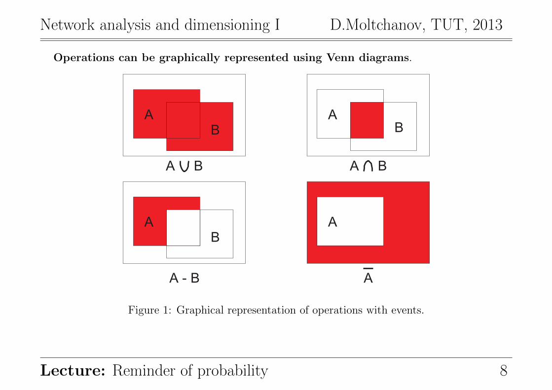
Operations can be graphically represented using Venn diagrams.

A

B

A

B

AA

B

A - B A

A B A B

Figure 1: Graphical representation of operations with events.



1.5. Events using set theory

Why we need to use set theory:

• set theory provide a natural way to describe events.

Define the following:

• Ω is a set of all outcomes associated with an experiment:

– also called sample space;

– for a die the sample space is given by:

Ω = 1, 2, 3, 4, 5, 6. (13)

• F is a set of subsets (σ-algebra) of Ω called events, such that:

– 0 ∈ F and Ω ∈ F ;

– if A ∈ F then the complementary set A ∈ F ;

– if An ∈ F , n = 1, 2, . . . , then⋃∞n=1An ∈ F .

– 2, 3, 5, 7, A1 = 2, A2 = 5: F = ∅, 2, 5, 3, 5, 7, 2, 3, 7, 2, 5, 3, 7,Ω.



2. Definitions of probability2.1. Classic definition

Assume we have experiment E generating a set of events F such that:

• events are mutually exclusive: when one occurs, others do not occur!

• events generate a full group:⋃ni=1Ai = Ω!

• events occur with equal chances: PrA1 = PrA2 = PrAn!

Note: these events can be just outcomes.

Definition: outcome w favors event A, if w leads to A.

Definition: probability of A:

• ratio of the number of outcomes favoring A to all number of outcomes.

Example: rolling a die, events A consists in getting even number:

• number of outcomes favoring A: m = 3; all number of outcomes: n = 6;

• probability of A: PrA = 3/6 = 1/2.



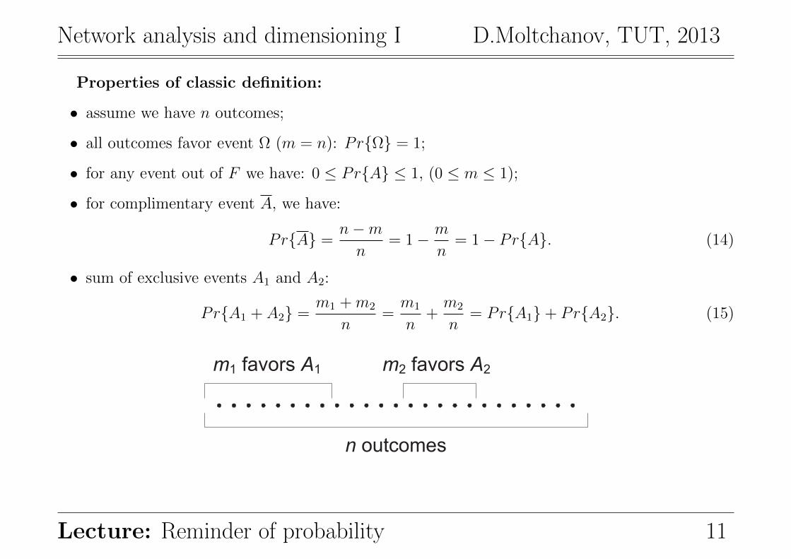
Properties of classic definition:

• assume we have n outcomes;

• all outcomes favor event Ω (m = n): PrΩ = 1;

• for any event out of F we have: 0 ≤ PrA ≤ 1, (0 ≤ m ≤ 1);

• for complimentary event A, we have:

PrA =n−mn

= 1− m

n= 1− PrA. (14)

• sum of exclusive events A1 and A2:

PrA1 + A2 =m1 +m2

n=m1

n+m2

n= PrA1+ PrA2. (15)

n outcomes

m1 favors A1 m2 favors A2



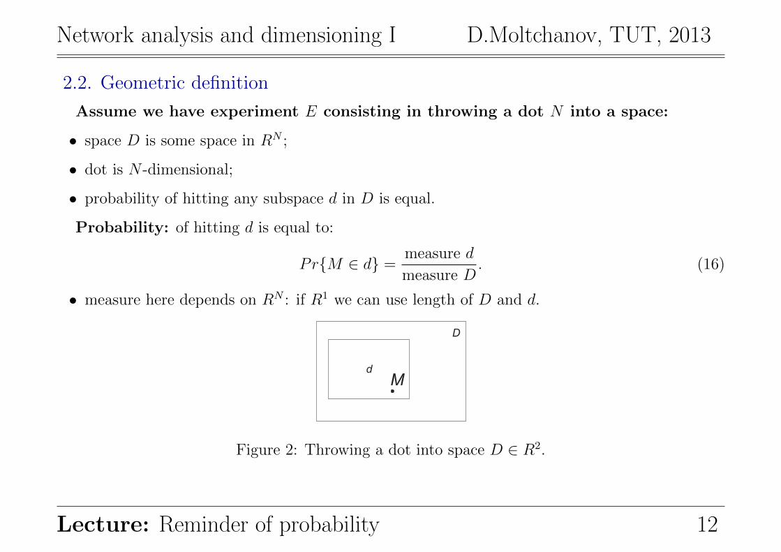
2.2. Geometric definition

Assume we have experiment E consisting in throwing a dot N into a space:

• space D is some space in RN ;

• dot is N -dimensional;

• probability of hitting any subspace d in D is equal.

Probability: of hitting d is equal to:

PrM ∈ d =measure d

measure D. (16)

• measure here depends on RN : if R1 we can use length of D and d.

D

d

M

Figure 2: Throwing a dot into space D ∈ R2.



2.3. Statistical definition

Why we need one more definition:

• classic and geometric definition have limited applicability;

• reason: it is not often possible to determine equally probable events.

Statistical definition:

• is known for centuries;

• stated by J. Bernoulli in his last work (1713);

• applicable to wide range of events: events with stable relative frequency.

Relative frequency of event A:

Pr?A = µ/n, (17)

• µ: number of experiments in which we observed A;

• n: whole number of experiments.



Definition: probability of event A is the value to which P ?A converges when n→∞.

PrA n→∞= Pr?A = µ/n. (18)

Note:

• statistical definition have the same properties as classic one;

• the only method to compute approximate probabilities if the experiment is not classic.

If outcomes are equally likely to occur we can use two methods:

• classic computation using PrA = m/n;

• using relative frequency: PrA n→∞= Pr?A = µ/n.

Buffon and Pearson compared number of heads in coin tossing:

n = 4040, m/n = 0.5, µ/n = 0.5080,

n = 12000, m/n = 0.5, µ/n = 0.5016,

n = 24000, m/n = 0.5, µ/n = 0.5005.

(19)



2.4. Axiomatic definition

Some facts:

• the most accepted definition;

• includes classic, geometric and statistical as special cases;

• introduced by A.N. Kolmogorov in 1933.

Let Ω be the set of outcomes, F be σ-algebra:

• P is a probability measure on (Ω, F ) such that:

– axiom 1: PA ≥ 0;

– axiom 2: PrΩ = 1;

– axiom 3: Pr0 = 0;

– axiom 4: Pr∑

k Ak =∑

k PrAk for mutually exclusive events..

Note: P is the a mapping from F in [0, 1].

Definition: (Ω, F, P ) is called the probability space.



3. Probability algebra

3.1. Adding events

For mutually exclusive events:

Pr

∑k

Ak

=∑k

PrAk. (20)

• holds only when events are exclusive!!!

For two arbitrary events:

PrA+B = PrA+ PrB − PrAB. (21)

For three arbitrary events:

PrA+B + C = PrA+ PrB − PrAB − PrBC − PrAC − PrABC. (22)

Note: one can extend it to n events.



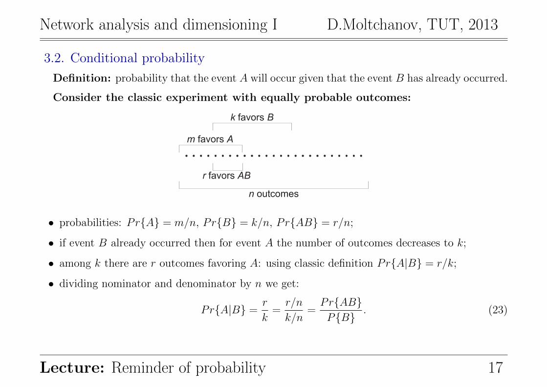
3.2. Conditional probability

Definition: probability that the event A will occur given that the event B has already occurred.

Consider the classic experiment with equally probable outcomes:

n outcomes

m favors A

k favors B

r favors AB

• probabilities: PrA = m/n, PrB = k/n, PrAB = r/n;

• if event B already occurred then for event A the number of outcomes decreases to k;

• among k there are r outcomes favoring A: using classic definition PrA|B = r/k;

• dividing nominator and denominator by n we get:

PrA|B =r

k=r/n

k/n=PrABPB

. (23)



Result:

PrA|B =PrABPB

. (24)

Note the following:

• one can check that P·|B is a probability measure;

• the conditional probability is not defined if PB = 0.

We can change the role of A and B:

P (B|A) =PABPA

. (25)

Example: there are three trunks:

• we seize the trunk with probability 1/3;

• what is the probability to seize a given trunk in two attempts?

• let: A: we seize the trunk in first attempt, B: we seize the trunk in second attempt:

PrA+ PrB − PrAB = 1/3 + 1/3− 1/9 = 5/9. (26)



3.3. Multiplication of events

Multiplication of two arbitrary events:

PrAB = PrBPrA|B = PrAPrB|A (27)

Multiplication of n arbitrary events:

PrA1A2 . . . An = PrA1PrA2|A1PrA3|A1A2 . . . P rAn|A1 . . . An−1. (28)

Multiplication of independent events:

PrA1A2 . . . An =n∏i=1

PrAi. (29)

Question:

• which events are dependent/independent?



3.4. Independent and dependent events

Definition: event A is independent of event B is the following holds:

PrA|B = PrA. (30)

• if one happens, it doesn’t affect the other one happening or not.

Examples:

• independent: getting tail/head tossing a coin;

• dependent: getting white ball out of the basket with red and white ones.

Note: if A is independent of B then B is independent of A.

Multiplication: if events A and B are independent then their product:

PrAB = PrBPrA|B = PrAPrB. (31)

Note: PrAB = PrAPrB is sufficient for events to be independent.



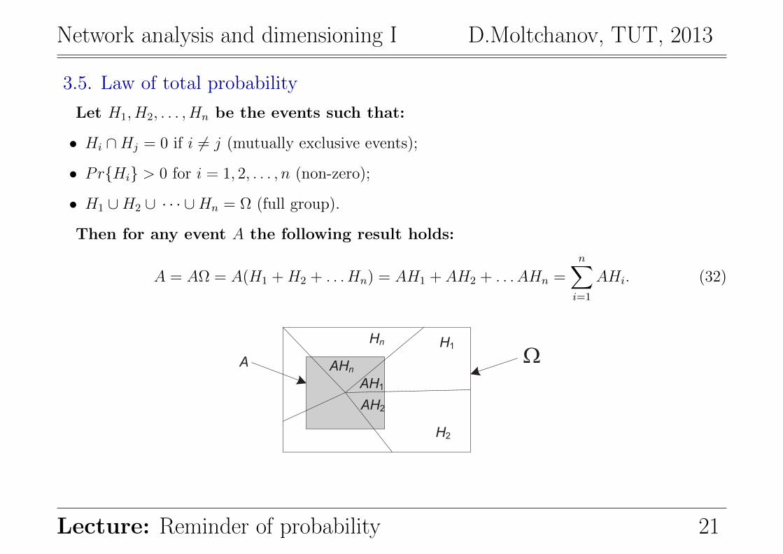
3.5. Law of total probability

Let H1, H2, . . . , Hn be the events such that:

• Hi ∩Hj = 0 if i 6= j (mutually exclusive events);

• PrHi > 0 for i = 1, 2, . . . , n (non-zero);

• H1 ∪H2 ∪ · · · ∪Hn = Ω (full group).

Then for any event A the following result holds:

A = AΩ = A(H1 +H2 + . . . Hn) = AH1 + AH2 + . . . AHn =n∑i=1

AHi. (32)

H1

H2

Hn

AH1

AH2

AHnA W



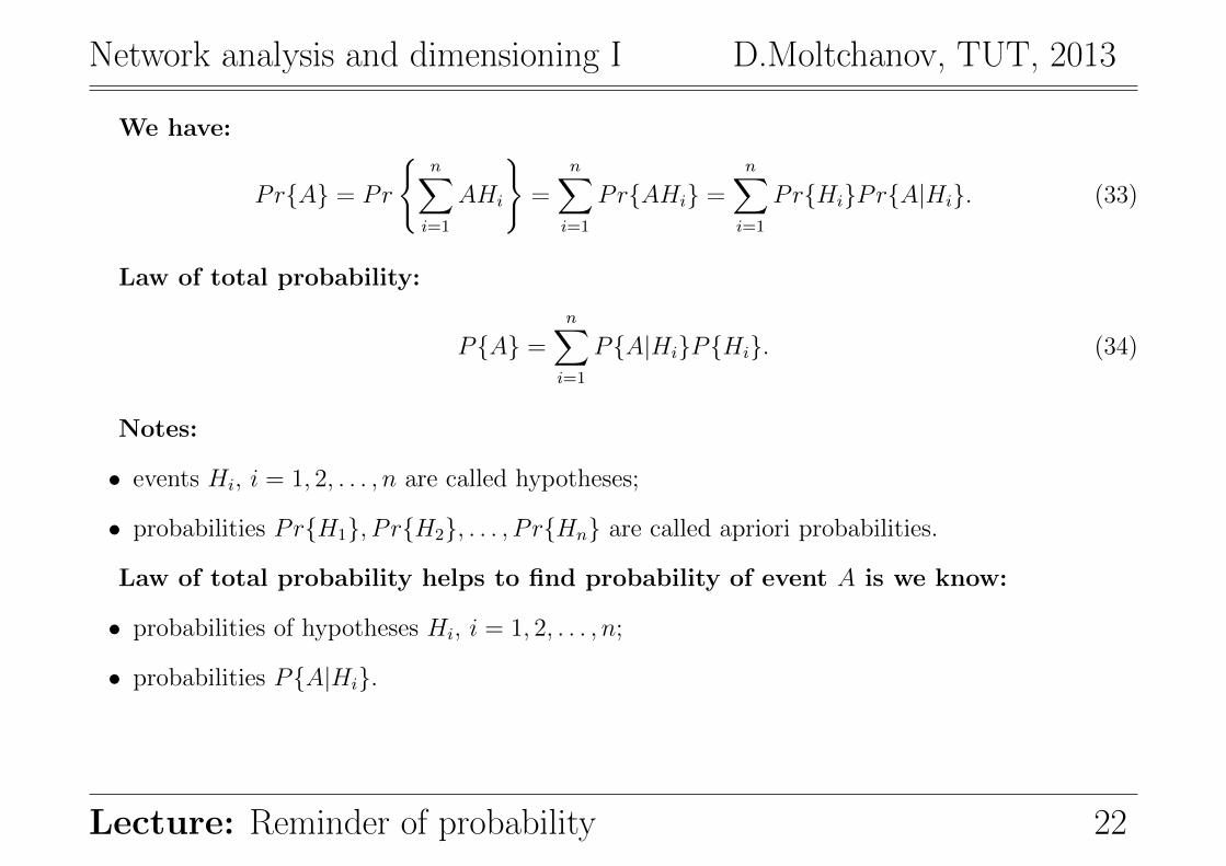
We have:

PrA = Pr

n∑i=1

AHi

=

n∑i=1

PrAHi =n∑i=1

PrHiPrA|Hi. (33)

Law of total probability:

PA =n∑i=1

PA|HiPHi. (34)

Notes:

• events Hi, i = 1, 2, . . . , n are called hypotheses;

• probabilities PrH1, P rH2, . . . , P rHn are called apriori probabilities.

Law of total probability helps to find probability of event A is we know:

• probabilities of hypotheses Hi, i = 1, 2, . . . , n;

• probabilities PA|Hi.



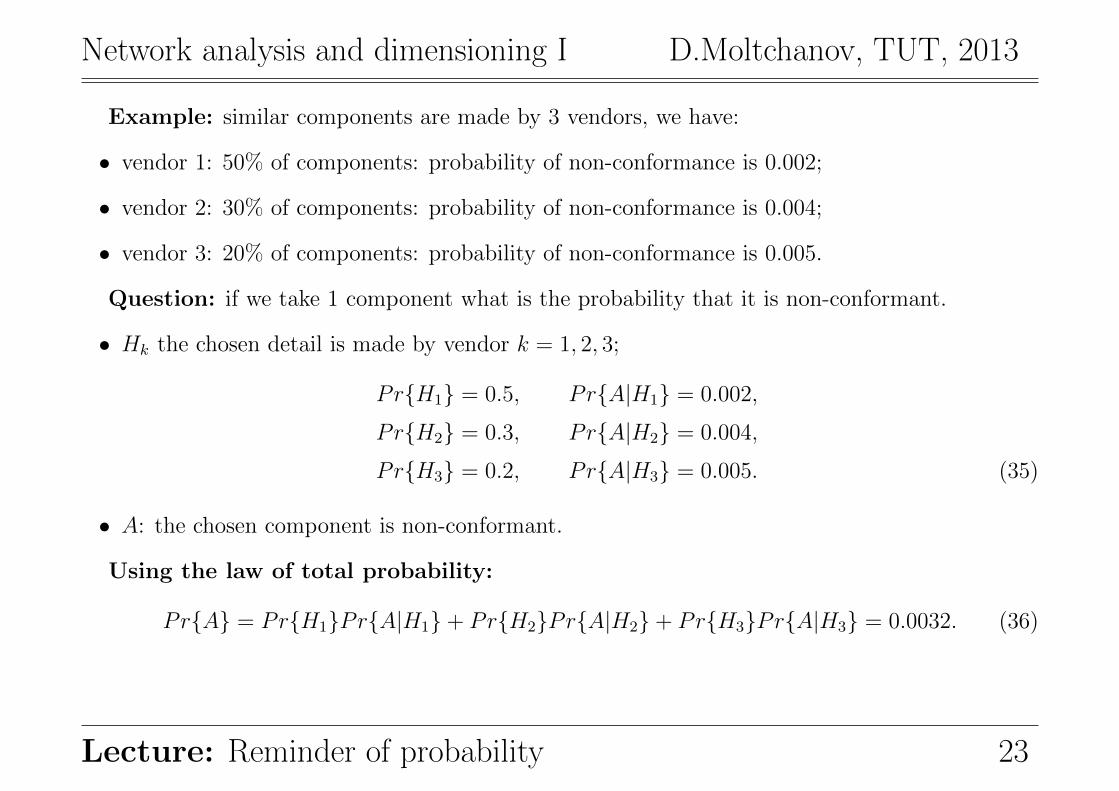
Example: similar components are made by 3 vendors, we have:

• vendor 1: 50% of components: probability of non-conformance is 0.002;

• vendor 2: 30% of components: probability of non-conformance is 0.004;

• vendor 3: 20% of components: probability of non-conformance is 0.005.

Question: if we take 1 component what is the probability that it is non-conformant.

• Hk the chosen detail is made by vendor k = 1, 2, 3;

PrH1 = 0.5, P rA|H1 = 0.002,

P rH2 = 0.3, P rA|H2 = 0.004,

P rH3 = 0.2, P rA|H3 = 0.005. (35)

• A: the chosen component is non-conformant.

Using the law of total probability:

PrA = PrH1PrA|H1+ PrH2PrA|H2+ PrH3PrA|H3 = 0.0032. (36)



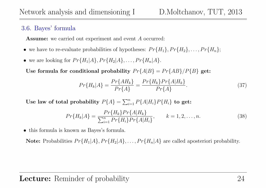
3.6. Bayes’ formula

Assume: we carried out experiment and event A occurred:

• we have to re-evaluate probabilities of hypotheses: PrH1, P rH2, . . . , P rHn;

• we are looking for PrH1|A, P rH2|A, . . . , P rHn|A.

Use formula for conditional probability PrA|B = PrAB/PB get:

PrHk|A =PrAHkPrA

=PrHkPrA|Hk

PrA. (37)

Use law of total probability PA =∑n

i=1 PA|HiPHi to get:

PrHk|A =PrHkPrA|Hk∑ni=1 PrHiPrA|Hi

, k = 1, 2, . . . , n. (38)

• this formula is known as Bayes’s formula.

Note: Probabilities PrH1|A, P rH2|A, . . . , P rHn|A are called aposteriori probability.



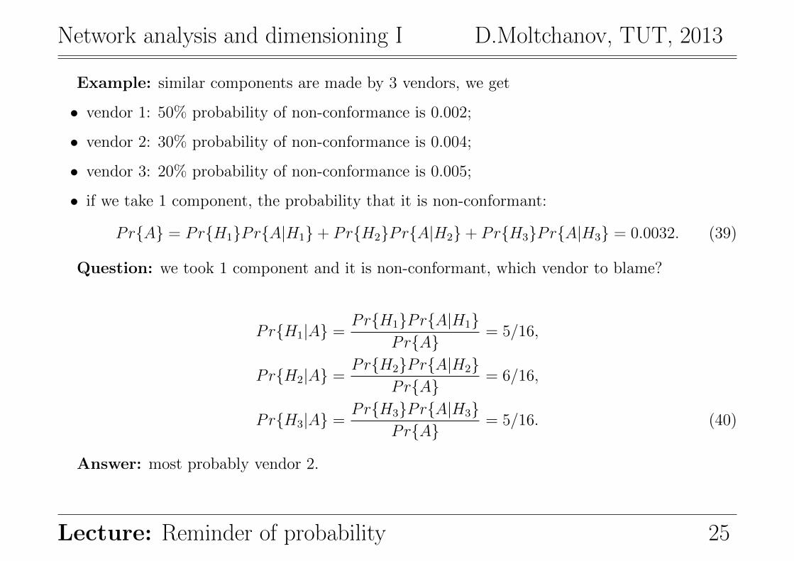
Example: similar components are made by 3 vendors, we get

• vendor 1: 50% probability of non-conformance is 0.002;



• if we take 1 component, the probability that it is non-conformant:

PrA = PrH1PrA|H1+ PrH2PrA|H2+ PrH3PrA|H3 = 0.0032. (39)

Question: we took 1 component and it is non-conformant, which vendor to blame?

PrH1|A =PrH1PrA|H1

PrA= 5/16,

P rH2|A =PrH2PrA|H2

PrA= 6/16,

P rH3|A =PrH3PrA|H3

PrA= 5/16. (40)

Answer: most probably vendor 2.



4. Random variablesBasic notes:

• events: sets of outcomes of the experiment;

• in many experiments we are interested in some number associated with the experiment:

• random variable: function which associates a number with experiment.

Examples:

• number of voice calls N that exists at the switch at time t:

– random variable which takes on integer values in (0, 1, . . . ,∞).

• service time ts of voice call at the switch:

– random variable which takes on any real value (0,∞).

Classification based on the nature of RV:

• continuous: R ∈ (−∞,∞);

• discrete: N ∈ 0, 1, . . . , Z ∈ . . . ,−1, 0, 1, . . . .



4.1. Special note

Random experiment:

• sample space: Ω;

• simple outcomes: ωi ∈ Ω, i = 1, 2, . . . ,M ;

• events we define: Ai, i = 1, 2, . . . , N ;

• σ-algebra: F , Ai ∈ F closed for complementarily nd union of Ai.

Question: where are these random numbers (variables) come from?

They appear:

• naturally: dice - Ω = 1, 2, 3, 4, 5, 6, X(ωi) = ωi;

• artificially: state is associated with a number X(ωi) = xi.

General formula: random variable X(ωi) = xi.



4.2. CDF, CCDF, pdf, and pmf

Definition: the probability that a random variable X is not greater than x:

F (x) = PrX ≤ x. (41)

• is called cumulative distribution function (CDF) of X.

Definition: complementary cumulative distribution function (CCDF) of RV X is:

FC(x) = PrX > x = 1− F (x). (42)

Definition: if X is a continuous RV, and F (x) is differentiable, then:

f(x) =dF (x)

dx, (43)

• is called probability density function (pdf).

Definition: if X is a discrete RV, then:

pj = PrX = j, (44)

• is called probability mass function (pmf) or probability function (PF).



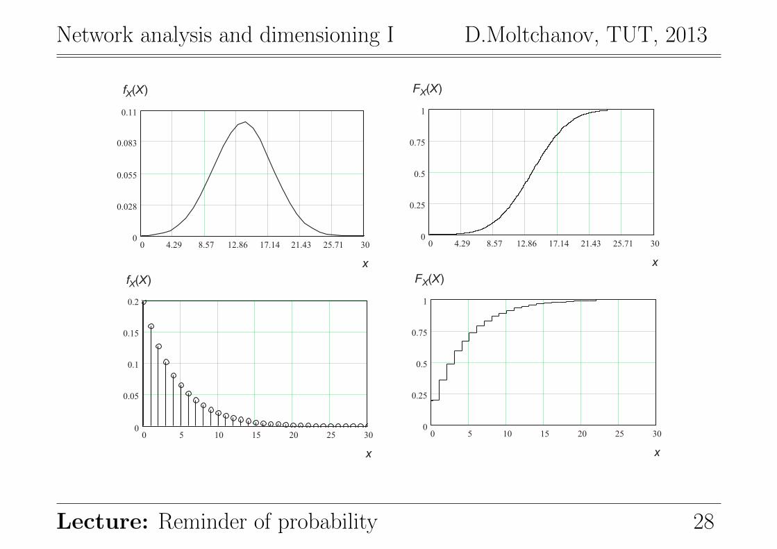
fX(X)

0 4.29 8.57 12.86 17.14 21.43 25.71 300

0.028

0.055

0.083

0.11

x

FX(X)

0 4.29 8.57 12.86 17.14 21.43 25.71 300

0.25

0.5

0.75

1

x

fX(X)

0 5 10 15 20 25 300

0.05

0.1

0.15

0.2

x

FX(X)

0 5 10 15 20 25 300

0.25

0.5

0.75

1

x



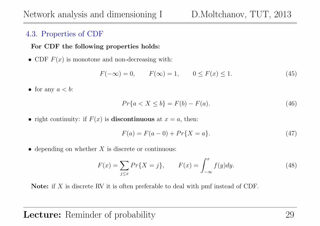
4.3. Properties of CDF

For CDF the following properties holds:

• CDF F (x) is monotone and non-decreasing with:

F (−∞) = 0, F (∞) = 1, 0 ≤ F (x) ≤ 1. (45)

• for any a < b:

Pra < X ≤ b = F (b)− F (a). (46)

• right continuity: if F (x) is discontinuous at x = a, then:

F (a) = F (a− 0) + PrX = a. (47)

• depending on whether X is discrete or continuous:

F (x) =∑j≤x

PrX = j, F (x) =

∫ x

−∞f(y)dy. (48)

Note: if X is discrete RV it is often preferable to deal with pmf instead of CDF.



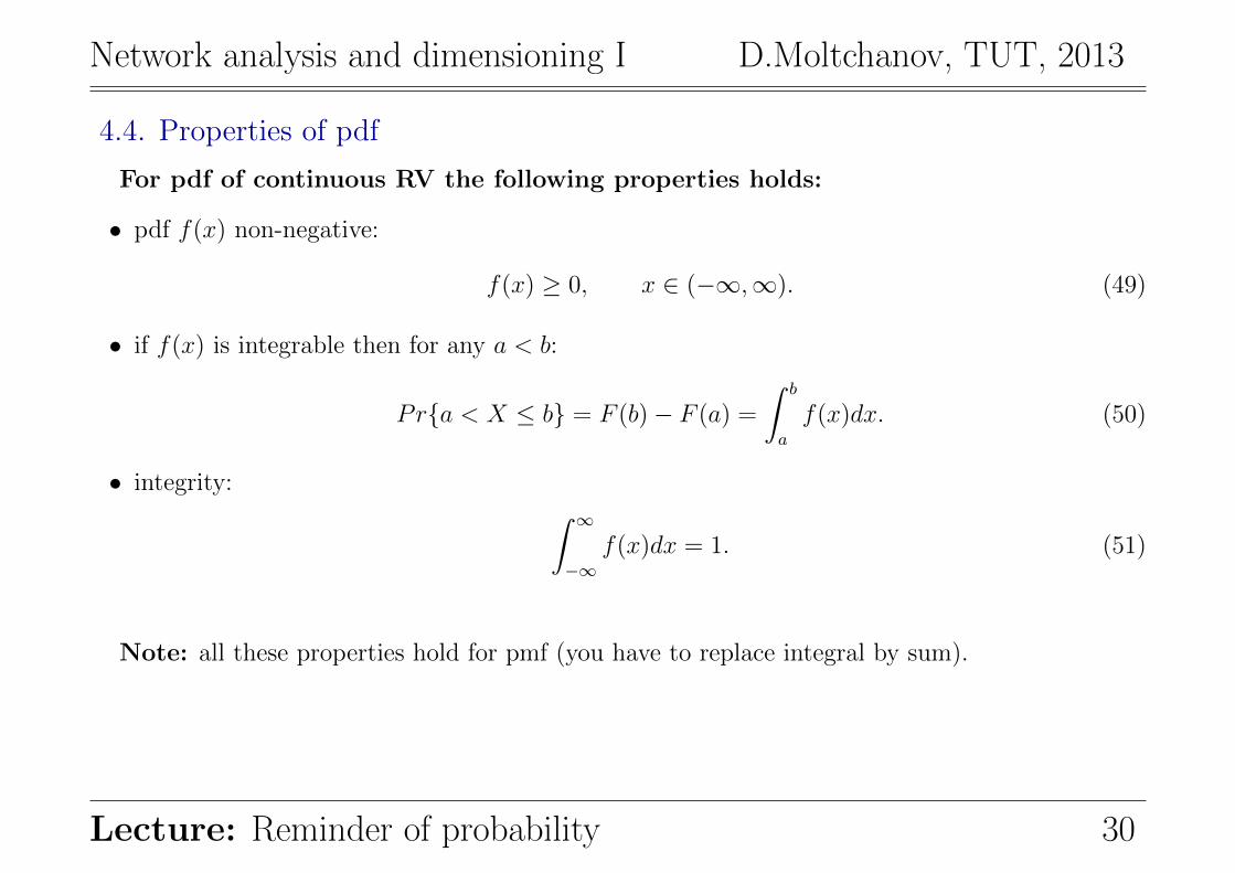
4.4. Properties of pdf

For pdf of continuous RV the following properties holds:

• pdf f(x) non-negative:

f(x) ≥ 0, x ∈ (−∞,∞). (49)

• if f(x) is integrable then for any a < b:

Pra < X ≤ b = F (b)− F (a) =

∫ b

a

f(x)dx. (50)

• integrity: ∫ ∞−∞

f(x)dx = 1. (51)

Note: all these properties hold for pmf (you have to replace integral by sum).



4.5. Parameters of RV

Basic notes:

• continuous RV: CDF and pdf give all information regarding properties of RV;

• discrete RV: CDF and pmf (PF) give all information regarding properties of RV.

Why we need something else:

• problem 1: CDF, pdf and pmf are sometimes not easy to deal with;

• problem 2: sometimes it is hard to estimate from data;

• solution: use parameters of RV.

What parameters:

• mean;

• variance;

• skewness;

• excess (sometimes called excess kurtosis), etc.



4.6. Mean

Definition: the mean of RV X is given by:

E[X] =∑∀i

xipi, E[X] =

∫ ∞−∞

xf(x)dx. (52)

• mean E[X] of RV X is between max and min value of non-complex RV:

minkxk ≤ E[X] ≤ max

kxk. (53)

• mean of the constant is constant:

E[c] = c. (54)

• mean of RV multiplied by constant value is constant value multiplied by the mean:

E[cX] = cE[X]. (55)

• mean of constant and RV X is the mean of X and constant value:

E[c+X] = c+ E[X]. (56)



4.7. Variance and standard deviation

Definition: the mean of the square of difference between RV X and its mean E[X]:

D[X] = E[(X − E[X])2]. (57)

How to compute variance:

• assume that X is discrete, compute variance as:

D[X] =∑∀n

(xn − E[X])2pn, (58)

• assume that X is continuous, compute variance as:

D[X] =

∫ ∞−∞

(x− E[X])2f(x)dx, (59)

• the another approach to compute variance:

D[X] = E[X2]− (E[X])2. (60)



Properties of the variance:

• the variance of the constant value is 0:

D[c] = E[(c− c)2] = E[0] = 0. (61)

• variance of RV multiplied by constant value:

D[cX] = E[(cX − cE[X])2] = E[c2(X − E[X])2] = c2D[X]. (62)

• variance of the constant value and RV X:

D[c+X] = E[((c+X)− (x+ E[X]))2] = E[(X − E[X])2] = D[X]. (63)

Definition: the standard deviation of RV X is given by:

σ[X] =√D[X]. (64)

Note: standard deviation is dimensionless parameter.



4.8. Other parameters: moments

Let us assume the following:

• X be RV (discrete or continuous);

• k ∈ 1, 2, . . . be the natural number;

• Y = Xk, Z = E[(X − E[X])k], k = 1, 2, . . . , be the set of random variables.

Assuming that X is continuous introduce the following functions:

• assume X is a discrete RV:

E[Xk] = E[Y ] =

∫ ∞−∞

xkfX(x)dx, (65)

– note: mean is obtained by setting k = 1.

• assume X is a continuous one.

E[(X − E[X])k] = E[Z] =

∫ ∞−∞

(x− E[X])kfX(x)dx, (66)

– note: variance is obtained by setting k = 2.



Definition: moment of order k of RV X is the mean of RV X in power of k:

αk = E[Xk]. (67)

Definition: central moment of order k of RV X is given by:

µk = E[(X − E[X])k]. (68)

One can note that:

E[X] = α1, D[X] = σ[X] = µ2 = α2 − α21. (69)

Definition: skewness of RV is given by:

sX =µ3

(σ[X])3. (70)

Definition: excess of RV is given by:

eX =µ3

(σ[X])4. (71)



4.9. Meaning of moments

Parameters meanings:

• measures of central tendency:

– mean: E[X] =∑∀i xipi;

– mode: value corresponding to the highest probability;

– median: value that equally separates weights of the distribution.

• measures of variability:

– variance: D[X] = E[(X − E[X])2];

– standard deviation:√D[X];

– squared coefficient of variation: k2X = D[X]/(E[X])2.

• other measures:

– skewness of distribution: skewness;

– excess of the mode: excess.

Note: not all parameters exist for a given distribution!





5. Jointly distributed RVsBasic notes:

• sometimes it is interesting to investigate two or more RVs;

• we assume that RVs X and Y are defined on some probability space.

Definition: joint cumulative distribution function (JCDF) of RVs X and Y is:

FXY (x, y) = PrX ≤ x, Y ≤ y. (72)

• for continuous RV.

Let us define:

FX(x) = PrX ≤ x, FY (y) = PrY ≤ y, x, y ∈ R, (73)

• FX(x) and FY (y) are called marginal CDFs.

Marginal CDF can be derived form JCDF:

FX(x) = limy→∞

F (x, y) = F (x,∞), FY (y) = limx→∞

F (x, y) = F (∞, y). (74)



Definition: if F (x, y) is differentiable then the following function:

fXY (x, y) =d2

dxdyFXY (x, y) = Prx ≤ X ≤ x+ dx, y ≤ Y ≤ y + dy, (75)

• is called joint probability density function (jpdf).

Assume then that X and Y are discrete RVs.

Definition: joint probability mass function (jmpf) of discrete RVs X and Y is:

FXY (x, y) = PrX = x, Y = x. (76)

Let us define:

FX(x) = PrX = x, FY (y) = PrY = y. (77)

• these functions are called marginal probability mass functions (mpmfs).

Marginal pmfs can be derived from jmpf:

FX(x) =∑∀y

FXY (x, y), FY (y) =∑∀x

FXY (x, y). (78)



5.1. Dependence and independence of RVs

Definition: if continuous RVs X and Y are independent then:

FXY (x, y) = FX(x)FY (y). (79)

• FX(x, y) is the JCDF;

• FX(x) and FY (y) are CDFs of RV X and Y .

Definition: if discrete RVs X and Y are independent then:

fXY (x, y) = fX(x)fY (y). (80)

• fXY (x, y) is the jpdf;

• fX(x) and fY (y) are pdfs of RV X and Y .

Definition: it is necessary and sufficient for two discrete RVs X and Y to be independent:

FXY (x, y) = FXY (X = x, Y = ∀)FXY (X = ∀, Y = y). (81)

• FX(x, y) is the jpmf;

• FX(x) and FY (y) are pmfs of RV X and Y .



5.2. Conditional distributions: measure of dependence

Definition: the following expression:

PrX|Y x|y = FX|Y (x|y) =PrX = ∀, Y = y

PrY = y, (82)

• gives conditional PF of discrete RV X given that Y = y.

Definition: the following expression:

fX|Y (x, y) =fXY (x, y)

fY (y), (83)

• gives conditional pdf of continuous RV X given that Y = y.

Conditional mean of RV X given Y = y from the following expression:

E[X|Y = y] =

∫ ∞−∞

xfX|Y (x|y)dx,

E[X|Y = y] =∑∀i

xiPrX|Y x, y. (84)

Note: not convenient to deal with as the metric is different for different (X, Y ).



5.3. Measure of dependence

Sometimes RVs are not independent:

• as a measure of dependence correlation moment (covariance) is used.

Definition: covariance of two RVs X and Y is defined as follows:

KXY = cov(X, Y ) = E[(X − E[X])(Y − E[Y ])]. (85)

• where from definition that KXY = KY X .

One can find the covariance using the following formulas:

• assume that RV X and Y are discrete:

KXY =∑i

∑j

(xi − E[X])(yj − E[Y ])PrX = xi, Y = yj,

(86)

• assume that RV X and Y are continuous:

KXY =

∫ ∞−∞

∫ ∞−∞

(xi − E[X])(yj − E[Y ])fXY (x, y)dxdy. (87)



It is often easy to use to following expression:

KXY = E[XY ]− E[X]E[Y ]. (88)

Problem with covariance: can be arbitrary in (−∞,∞):

• problem: hard to compare dependence between different pair of RVs;

• solution: use correlation coefficient to measure the dependence between RVs.

Definition: correlation coefficient of RVs X and Y is defined as follows:

ρXY =KXY

σ[X]σ[Y ]. (89)

• −1 ≤ ρXY ≤ 1;

• if ρXY 6= 0 then RVs X and Y are dependent;

• assume we are given RVs X and Y such that Y = aX + b:

ρXY = +1, a > 0,

ρXY = −1, a < 0. (90)



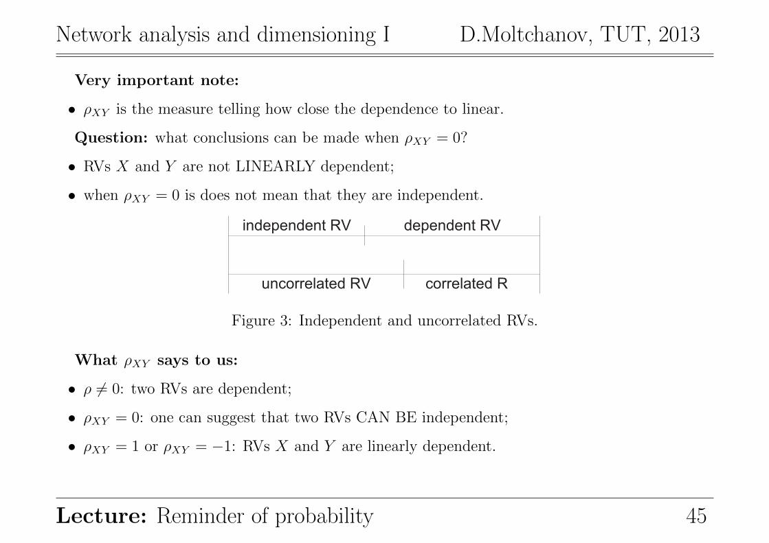
Very important note:

• ρXY is the measure telling how close the dependence to linear.

Question: what conclusions can be made when ρXY = 0?

• RVs X and Y are not LINEARLY dependent;

• when ρXY = 0 is does not mean that they are independent.

independent RV dependent RV

uncorrelated RV correlated R

Figure 3: Independent and uncorrelated RVs.

What ρXY says to us:

• ρ 6= 0: two RVs are dependent;

• ρXY = 0: one can suggest that two RVs CAN BE independent;

• ρXY = 1 or ρXY = −1: RVs X and Y are linearly dependent.



5.4. Sum and product of correlated RVs

Mean:

• the mean of the product of two correlated RVs:

E[XY ] = E[X]E[Y ] +KXY . (91)

• the mean of the product of two uncorrelated RVs:

E[XY ] = E[X]E[Y ]. (92)

Variance:

• the variance of the sum of two correlated RVs:

D[X + Y ] = D[X] +D[Y ] + 2KXY . (93)

• the variance of the sum of two uncorrelated RVs:

D[X + Y ] = D[X] +D[Y ]. (94)



5.5. pdf and pmf of the sum of arbitrary RVs

Basic note:

• pdf of the sum of two independent RVs can be obtained using convolution operation.

We consider independent RVs X and Y with pmfs:

mX(x) = PrX = x, mY (y) = PrY = y. (95)

pmf of RV Z, Z = X + Y is defined as follows:

PrZ = z =∞∑

k=−∞

PrX = kPrY = z − k. (96)

• if X = k, then, Z take on z (Z = z) if and only if Y = z − k.

If RVs X and Y are continuous:

fX(x) fY (y) =

∫ ∞−∞

fX(z − y)fY (y)dy =

∫ ∞−∞

fY (z − x)fX(x)dx. (97)



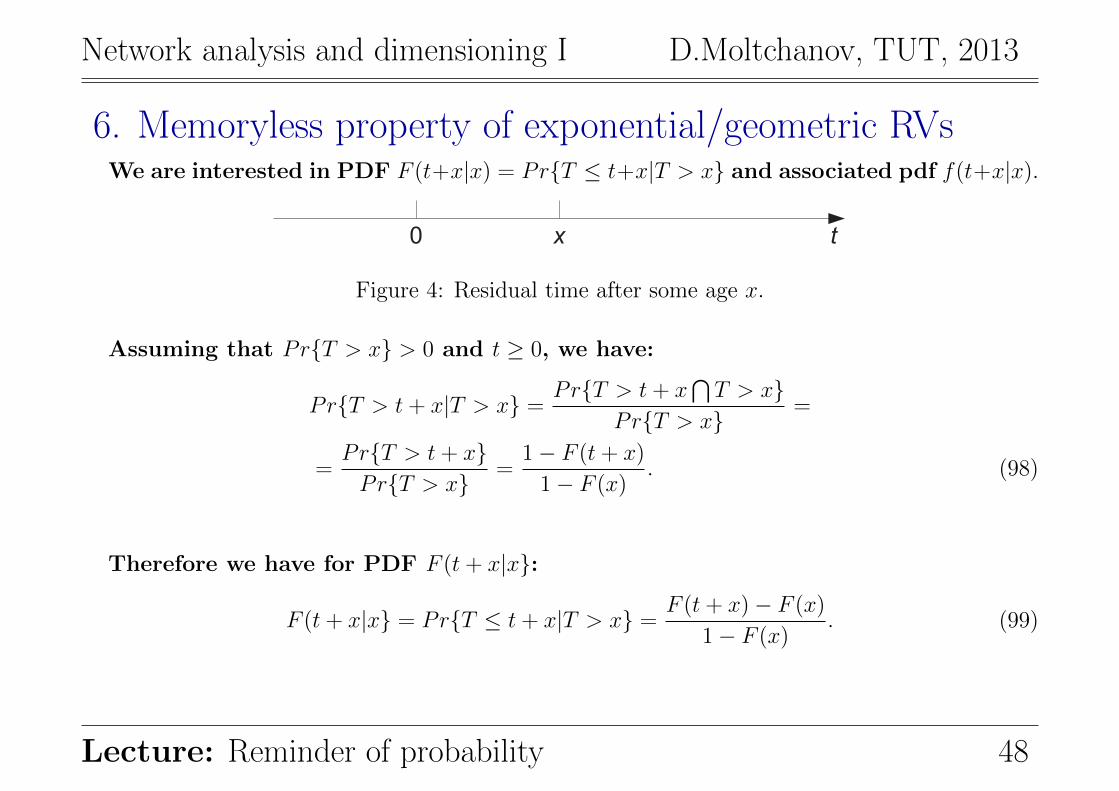
6. Memoryless property of exponential/geometric RVsWe are interested in PDF F (t+x|x) = PrT ≤ t+x|T > x and associated pdf f(t+x|x).

x t0

Figure 4: Residual time after some age x.

Assuming that PrT > x > 0 and t ≥ 0, we have:

PrT > t+ x|T > x =PrT > t+ x

⋂T > x

PrT > x=

=PrT > t+ xPrT > x

=1− F (t+ x)

1− F (x). (98)

Therefore we have for PDF F (t+ x|x:

F (t+ x|x = PrT ≤ t+ x|T > x =F (t+ x)− F (x)

1− F (x). (99)



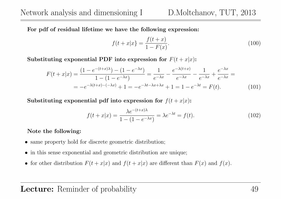
For pdf of residual lifetime we have the following expression:

f(t+ x|x =f(t+ x)

1− F (x). (100)

Substituting exponential PDF into expression for F (t+ x|x):

F (t+ x|x) =(1− e−(t+x)λ)− (1− e−λx)

1− (1− e−λx)=

1

e−λx− e−λ(t+x)

e−λx− 1

e−λx+e−λx

e−λx=

= −e−λ(t+x)−(−λx) + 1 = −e−λt−λx+λx + 1 = 1− e−λt = F (t). (101)

Substituting exponential pdf into expression for f(t+ x|x):

f(t+ x|x) =λe−(t+x)λ

1− (1− e−λx)= λe−λt = f(t). (102)

Note the following:

• same property hold for discrete geometric distribution;

• in this sense exponential and geometric distribution are unique;

• for other distribution F (t+ x|x) and f(t+ x|x) are different than F (x) and f(x).



7. Important distributionsWe will deal with:

• discrete distributions:

– Bernoulli;

– geometric;

– binomial;

– Poisson.

• continuous distributions:

– exponential;

– normal.

Next we have a short overview for reference purposes:

• pmf or pdf or CDF;

• moments: mean, variance;

• graphical illustration.



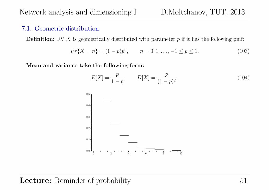
7.1. Geometric distribution

Definition: RV X is geometrically distributed with parameter p if it has the following pmf:

PrX = n = (1− p)pn, n = 0, 1, . . . ,−1 ≤ p ≤ 1. (103)

Mean and variance take the following form:

E[X] =p

1− p, D[X] =

p

(1− p)2. (104)



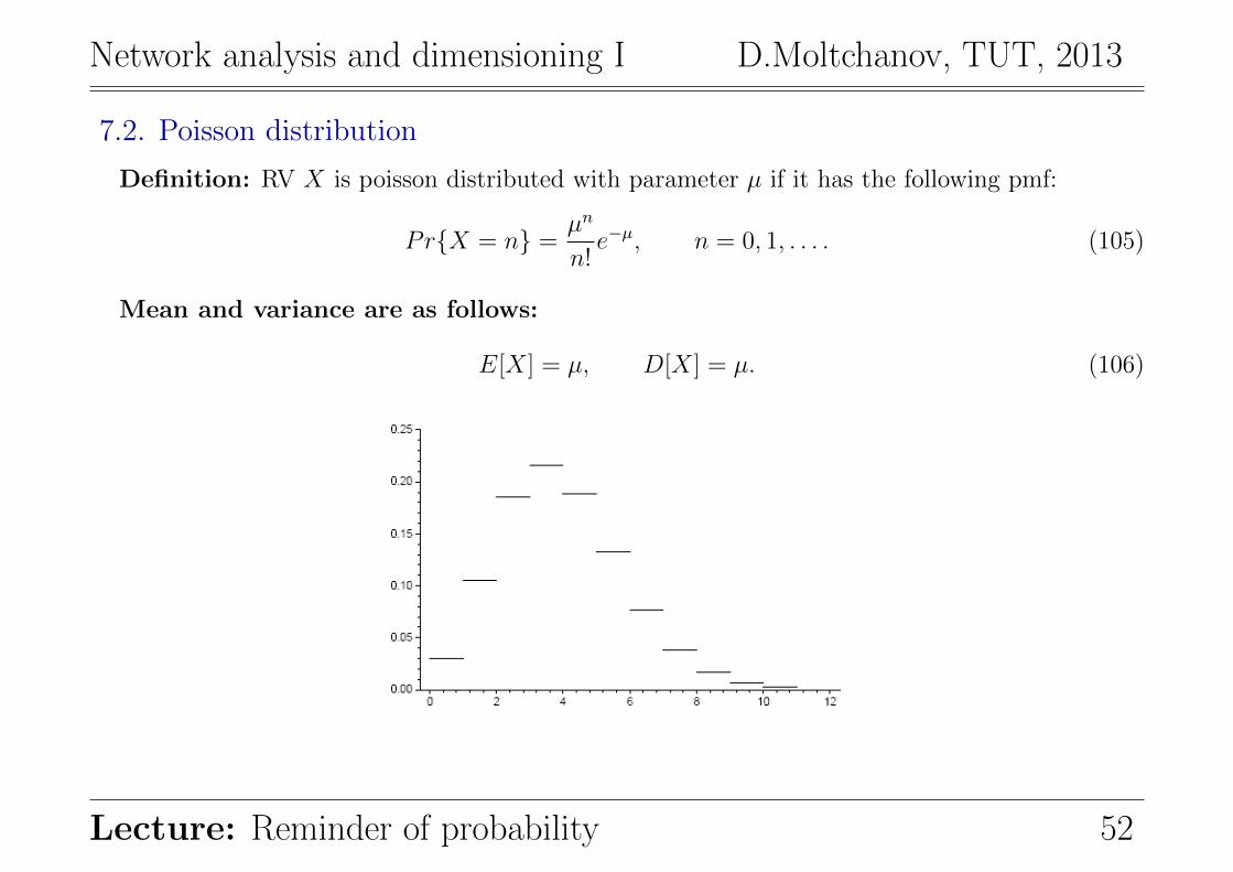
7.2. Poisson distribution

Definition: RV X is poisson distributed with parameter µ if it has the following pmf:

PrX = n =µn

n!e−µ, n = 0, 1, . . . . (105)

Mean and variance are as follows:

E[X] = µ, D[X] = µ. (106)



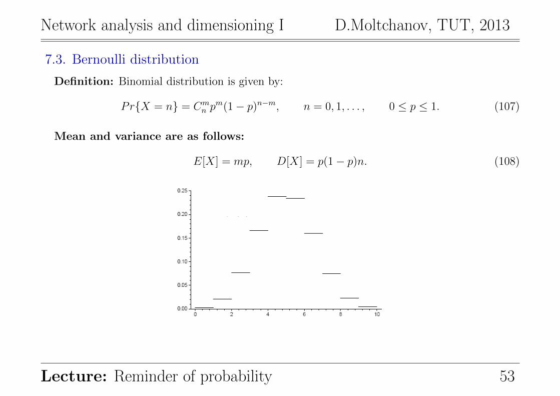
7.3. Bernoulli distribution

Definition: Binomial distribution is given by:

PrX = n = Cmn p

m(1− p)n−m, n = 0, 1, . . . , 0 ≤ p ≤ 1. (107)


E[X] = mp, D[X] = p(1− p)n. (108)



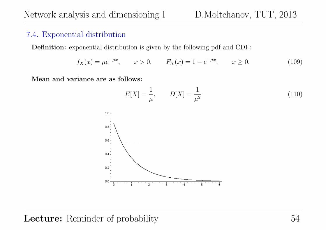
7.4. Exponential distribution

Definition: exponential distribution is given by the following pdf and CDF:

fX(x) = µe−µx, x > 0, FX(x) = 1− e−µx, x ≥ 0. (109)


E[X] =1

µ, D[X] =

1

µ2(110)



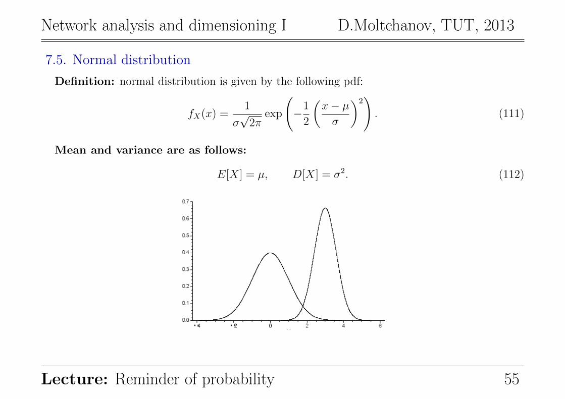
7.5. Normal distribution

Definition: normal distribution is given by the following pdf:

fX(x) =1

σ√

2πexp

(−1

2

(x− µσ

)2). (111)


E[X] = µ, D[X] = σ2. (112)



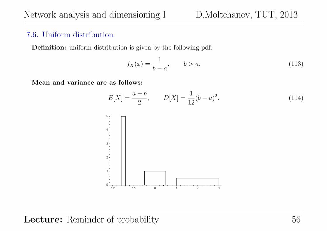
7.6. Uniform distribution

Definition: uniform distribution is given by the following pdf:

fX(x) =1

b− a, b > a. (113)


E[X] =a+ b

2, D[X] =

1

12(b− a)2. (114)



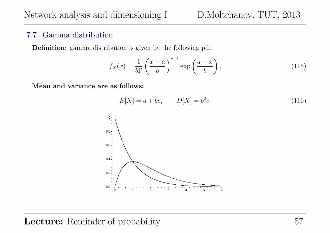
7.7. Gamma distribution

Definition: gamma distribution is given by the following pdf:

fX(x) =1

bΓ

(x− ab

)c−1exp

(a− xb

). (115)


E[X] = a+ bc, D[X] = b2c. (116)


Documents

Reminder of probability - TUT · ratio of the number of outcomes favoring Ato all number of outcomes. ... PrfAgn!1= Pr?fAg= =n: ... Reminder of probability 14