Remediation of Acid Mine Drainage utilizing sugar cane

1

Remediation of Acid Mine Drainage utilizing

sugar cane bagasse and basic oxygen furnace

slag

Jarad Hadley Dusterwald

A dissertation submitted to the Faculty of Engineering and the Built Environment, University

of the Witwatersrand, Johannesburg, in fulfilment of the requirements for the degree of

Master of Science in Engineering.

Johannesburg, 2019

2

Declaration

I declare that this dissertation is my own unaided work. It is being submitted to the degree of

Master of Science in Engineering to the University of the Witwatersrand, Johannesburg. It

has not been submitted before for any other degree or examination in any other University.

_______________________ Jarad Hadley Dusterwald

23rd of August 2019

3

Abstract

In this study a combination of basic oxygen furnace (BOF) slag and sugar cane bagasse (SCB)

were assessed for their potential to remediate acid mine drainage (AMD). SCB was also

individually assessed to determine its remedial potential.

Small-scale laboratory experiments were carried out to determine the effectiveness of this

combination of BOF slag and SCB in removing sulfate and iron and raising the pH. In the

small-scale laboratory experiments, four different configurations were used: the first

configuration was packed with SCB in the first column and SCB in the second column, the

second configuration was packed with SCB in the first column and BOF slag in the second

column, the third configuration was packed with a mixture of SCB and BOF slag in the first

and second columns and the fourth configuration was packed with BOF slag in the first column

and SCB in the second column. The results that followed indicated that there is a potential for

SCB and BOF slag to treat AMD.

These experiments occurred for two different residence times; a low residence time which was

approximately 35.5 hours ± 5.5 and a high residence time which was approximately 78.5 hours

± 7.5. The removal of iron and sulfate as well as the increase in pH showed that all the

configurations achieved some form of remediation. The highest percentage of sulfate removed

in all the configurations was 86%, the highest percentage of iron removed was 99.99% and the

highest pH value at the outlet was 12.82; all of these maxima were achieved for the higher

residence times, indicating the impact that residence time has on these particular systems.

A one-way analysis of variance (ANOVA) within each of the configurations, and variance

between the configurations was performed on the resulting data using the built-in function in

Excel; this was done within the 95% confidence interval. These tests indicated that there was

a statistical significance, when it came to raising the pH and removing iron between the

columns that had no BOF slag and the columns that did, and by interpreting the graphs in the

results section, it can be seen that it was the BOF slag that was responsible for the higher rise

in the pH and for most columns the higher removal of iron. Initially indications appear to be

4

optimal for configuration D (the first column containing BOF slag and the second column

containing SCB) being the most suited to treat AMD, however when the residence times were

taken into account and the results found in Section 4 and ANOVA were interpreted more

thoroughly, it gave an indication that configuration B (the first column containing SCB and the

second column containing BOF slag) is the most suited to treating AMD. Configuration B has

a high removal percentage of sulfate of 67% and maintains a removal of sulfate for over 55%

for a longer period of time than configuration D. The start of breakthrough for configuration B

took longer than that of any other configurations and as such the replacement of the remediating

substances would not be as frequent.

The results show that these materials are able to treat synthetic AMD. They also show that the

interoperating of BOF slag and SCB is better than the configuration containing only SCB.

Results also indicate that higher residence times are more suited to treating AMD in removing

a higher percentage of iron, sulfate and raising the pH. The results also indicate that

configuration B is the most suited to treat AMD.

5

Dedication

To my family; quae familia est.

6

Acknowledgments

I would like to acknowledge my supervisors: Professors Craig Sheridan and Lizelle Van Dyk,

your patience and kindness throughout this project have been invaluable.

To Dr Dennis Grubb, Iwan Vermeulen and Phoenix slags for their help and resources.

To my brother Joshua Keith Evan White who helped in so many ways.

To my wife Saffiya Dusterwald: thank you for your patience and help.

To my father Hardy Dusterwald for helping me with the review.

To Dr David Rose for the help on ANOVA.

To the workshop at the University of Witwatersrand thank you all.

7

Table of contents

Declaration 2

Abstract 3

Dedication 5

Acknowledgments 6

Nomenclature 15

1 Introduction 17

1.1 Background 17

1.2 Problem statement 19

1.3 Research objectives 19

1.4 Dissertation layout 19

2 Literature review 21

2.1 Introduction 21

2.2 Overview of acid mine drainage 21

2.3 Stability of acid mine drainage compounds 23

2.4 Environmental impact 25

2.4.1 Impacts on human health 25

2.4.3 Impact on physical environment 27

2.4.4 Impact on aquatic life 28

2.5 Review of acid mine drainage remediation options 30

2.5.1 Prevention 31

2.5.2 Active treatment 33

2.5.1.1 Membrane separation 35

2.5.1.2 High density sludge process 36

2.5.1.3 pH Neutralisation Reagents 37

2.5.3 Passive remediation technique 38

2.5.2.1 Constructed Wetlands 38

2.5.2.2 Packed reactor bed 39

2.5.4 Reducing and Alkalinity Producing Systems 39

2.6 Water codes and restrictions in the South African context 40

8

2.6.1 Standards and restrictions 40

2.6.2 Acid mine drainage impact on the Witbank environment 42

2.7 Overview of Sugar cane bagasse 42

2.8 Overview of Sulfate reducing bacteria and their use 44

2.8.1 Sulfur and iron oxidizing microorganisms 46

2.9 Overview of basic oxygen furnace slags and the application of basic oxygen furnace

slag in acid mine drainage remediation 46

2.10 Conclusion 49

3 Experimental Material and Methods 51

3.1 Introduction 51

3.2 Experimental 51

3.2.1 Description of experimental apparatus 51

3.3 Materials 55

3.3.1 Sugar cane bagasse 55

3.3.2 Basic oxygen furnace slag 55

3.3.3 Simulated acid mine drainage 55

3.4 Experimental Procedure 56

3.4.1 Column packing and sulfate reducing bacteria pre-treatment 56

3.4.2 Acid mine drainage in different process configurations 56

3.4.3 Sampling protocol 57

3.4.3.1 Analytical techniques 58

4 Results 61

4.1 Characterization of slag 61

4.2 Initial acid mine drainage treatment results for different process configurations at 12 h

column residence times. 64

4.3 Acid mine drainage Treatment in process Configuration A (bagasse and bagasse

columns) 66

4.3.1 Treatment of acid mine drainage at high flow in configuration A (τ = 34 hours) 67

4.3.2 Treatment of acid mine drainage at low flow in configuration A (τ = 83 hours) 74

4.3.3 Comparison of low and high flow treatment of AMD in process configuration A 82

4.4 Acid mine drainage Treatment in process Configuration B (Bagasse and BOF slag

columns) 83

9

4.4.1 Treatment of acid mine drainage at high flow in configuration B (τ = 30 hours) 83

4.4.2 Treatment of acid mine drainage at low flow in configuration B (τ = 71 hours) 93

4.4.3 Comparison of low and high flow treatment of AMD in process configuration B

101

4.5 Acid mine drainage Treatment in process Configuration C (Bagasse and BOF Slag

Mixed Columns) 101

4.5.1 Treatment of acid mine drainage at high flow in configuration C (τ = 41 hours) 102

4.5.2 Treatment of acid mine drainage at low flow in configuration C (τ = 79 hours) 111

4.5.3 Comparison of low and high flow treatment of AMD in process configuration C

118

4.6 Acid mine drainage Treatment in process Configuration D (BOF slag and Bagasse

Columns) 119

4.6.1 Treatment of acid mine drainage at high flow in configuration D (τ = 37 hours) 120

4.6.2 Treatment of acid mine drainage at low flow in configuration D (τ = 86 hours) 128

4.6.3 Comparison of low and high flow treatment of AMD in process configuration D

136

4.7 Analysis of variance section: Comparison of the Configurations 137

4.7.1 Analysis of variance comparison of all configuration, high flow 137

4.7.2 Analysis of variance comparison of all configuration, low flow 139

4.8 Comparison of best results considering residence times 142

5 Discussion and conclusion 145

Reference 149

Appendix A 168

Appendix B 174

Appendix C 179

10

List of Figures

Figure 2.1: Pourbaix diagram for the iron-sulfur-water system at 298 K (Rose, 2010) .......... 24

Figure 2.2: Remediation techniques for AMD (Johnson and Hallberg, 2002) ........................ 31

Figure 2.3: AMD formation minimization and prevention techniques (Johnson and Hallberg,

2002) ........................................................................................................................................ 32

Figure 3.1: Photograph depicting the experimental set up in the lab ....................................... 52

Figure 3.2: Schematic of experimental apparatus for configuration A .................................... 53

Figure 3.3: Schematic of experimental apparatus for configuration B .................................... 53

Figure 3.4: Schematic of experimental apparatus for configuration C .................................... 54

Figure 3.5: Schematic of experimental apparatus for configuration D .................................... 54

Figure 4.1: BOF slag; the used slag is on the left whilst looking at the picture and the unused

BOF slag is on the right ........................................................................................................... 63

Figure 4.2: BOF slag; the used slag is on the left whilst looking at the picture and the unused

BOF slag is on the right ........................................................................................................... 63

Figure 4.3:SCB, Unused SCB on the left and used SCB on the right ..................................... 64

Figure 4.4: Outlet pH of the various configurations for 24-hour residence time (very high

flow) ......................................................................................................................................... 65

Figure 4.5: Schematic of Configuration A- two bagasse columns in series ............................ 67

Figure 4.6: pH as a function of pore volumes for configuration A (bagasse and bagasse

columns, 34-hour residence time) ............................................................................................ 68

Figure 4.7: Sulfate concentration as a function of pore volume for configuration A (bagasse

and bagasse columns, 34-hour residence time) ........................................................................ 69

Figure 4.8: Percentage sulfate removed as a function of PV for configuration A (bagasse and

bagasse columns, 34-hour residence time) .............................................................................. 71

Figure 4.9: Dissolved Iron concentration as a function of PV for configuration A (bagasse


Figure 4.10: Percentage dissolved Iron removed as a function of PV for configuration A

(bagasse and bagasse columns, 34-hour residence time) ......................................................... 73

Figure 4.11: Outlet pH as a function of PV for configuration A (bagasse and bagasse


Figure 4.12: Sulfate concentration as a function of PV for configuration A (bagasse and

bagasse columns, 83-hour residence time) .............................................................................. 76

Figure 4.13: Percentage Sulfate removed as a function of PV for configuration A (bagasse


Figure 4.14: Iron concentration as a function of PV for configuration A (bagasse and .......... 79

11

Figure 4.15: Percentage Total iron removed as a function of PV for configuration A (bagasse


Figure 4.16: Calcium as a function of PV for configuration A (bagasse and bagasse columns,

83-hour residence time) ........................................................................................................... 81

Figure 4.17: Schematic of Configuration B- Bagasse column followed by a BOF slag column.

.................................................................................................................................................. 83

Figure 4.18: Outlet pH as a function of PV for configuration B (bagasse and BOF slag


Figure 4.19: Sulfate concentration as a function of PV for configuration B (bagasse and BOF

slag columns, 30-hour residence time) .................................................................................... 86

Figure 4.20: Percentage Sulfate removed as a function of PV for configuration B (bagasse

and BOF slag columns, 30-hour residence time) ..................................................................... 87

Figure 4.21: Dissolved Iron concentration as a function of PV for configuration B (bagasse


Figure 4.22: Percentage Dissolved Iron removed as a function of PV for configuration B

(bagasse and BOF slag columns, 30-hour residence time) ...................................................... 89

Figure 4.23: SEM results for fresh (unused) BOF slag, 1000 X magnification ...................... 91

Figure 4.24: SEM results for configuration B, used BOF slag, 1000 X magnification ........... 91



Figure 4.26: Sulfate concentration as a function of PV for configuration B (bagasse and BOF


Figure 4.27: Percentage Sulfate removed as a function of PV for configuration B (bagasse


Figure 4.28: Iron concentration as a function of PV for configuration B (bagasse and BOF


Figure 4.29: Percentage Total Iron removed as a function of PV for configuration B (bagasse


Figure 4.30: Calcium as a function of PV for configuration B (bagasse and BOF slag


Figure 4.31: Schematic of Configuration C- two bagasse and BOF slag mixed columns in

series ...................................................................................................................................... 102

Figure 4.32: Outlet pH as a function of PV for configuration C (bagasse and BOF slag mixed

columns, 41-hour residence time) .......................................................................................... 103

Figure 4.33: Sulfate concentration as a function of PV for configuration C (bagasse and BOF

slag mixed columns, 41-hour residence time) ....................................................................... 104

Figure 4.34: Percentage Sulfate removed as a function of PV for configuration C (bagasse

and BOF slag mixed columns, 41-hour residence time) ........................................................ 105

Figure 4.35: Dissolved Iron concentration as a function of PV for configuration C (bagasse


12

Figure 4.36: Percentage Dissolved Iron removed as a function of PV for configuration C

(bagasse and BOF slag mixed columns, 41-hour residence time) ......................................... 107

Figure 4.37: SEM results for fresh (unused) BOF slag, 1000 X magnification .................... 108

Figure 4.38: SEM results for configuration C, used BOF slag from the first column, 1000 X

magnification ......................................................................................................................... 108

Figure 4.39: SEM results for configuration C, used BOF slag from the second column, 1000

X magnification ..................................................................................................................... 109

Figure 4.40: Outlet pH as a function of PV for configuration C (bagasse and BOF slag

mixed column, 79-hour residence time) ................................................................................ 112

Figure 4.41: Sulfate concentration as a function of PV for configuration C (bagasse and BOF


Figure 4.42: Percentage Sulfate removed as a function of PV for configuration C (bagasse


Figure 4.43: Iron concentration as a function of PV for configuration C (bagasse and BOF


Figure 4.44: Percentage Total Iron removed as a function of PV for configuration C (bagasse


Figure 4.45: Calcium as a function of PV for configuration C (bagasse and BOF slag mixed


Figure 4.46: Schematic of Configuration D- BOF slag column followed by bagasse column

................................................................................................................................................ 120

Figure 4.47: Outlet pH as a function of PV for configuration D (BOF slag and bagasse


Figure 4.48: Sulfate concentration as a function of PV for configuration D (BOF slag and

bagasse columns, 37-hour residence time) ............................................................................ 122

Figure 4.49: Percentage Sulfate removed as a function of PV for configuration D (BOF slag

and bagasse columns, 37-hour residence time) ...................................................................... 123

Figure 4.50: Dissolved Iron concentration as a function of PV for configuration D (BOF slag


Figure 4.51: Percentage Dissolved Iron removed as a function of PV for configuration D

(BOF slag and bagasse columns, 37-hour residence time) .................................................... 125

Figure 4.52: SEM results for fresh (unused) BOF slag, 1000 X magnification .................... 126

Figure 4.53: SEM results for configuration D, used BOF slag, 1000 X magnification......... 126



Figure 4.55: Sulfate concentration as a function of PV for configuration D (BOF slag and


Figure 4.56: Percentage Sulfate removed as a function of PV for configuration D (BOF slag


13

Figure 4.57: Iron concentration as a function of PV for configuration D (BOF slag and


Figure 4.58: Percentage Total Iron removed as a function of PV for configuration D (BOF

slag and bagasse columns, 86-hour residence time) .............................................................. 134

Figure 4.59: Calcium as a function of PV for configuration D (bagasse and BOF slag


List of Tables Table 2.1: Some metal sulfides attributed to AMD formation (Simate et al., 2014; Skousen et

al., 1998) .................................................................................................................................. 22

Table 2.2: Heavy metals, their effect on human health and their permissible levels (Singh et

al., 2011; Solomon, 2008; Monachese et al., 2012) ................................................................. 26

Table 2.3: Heavy metal impacts on plants (Gardea-Torresdey et al., 2005; Akpor and Muchie,

2010; Yadav, 2010) .................................................................................................................. 27

Table 2.4: Permissible levels of heavy metals concerning protection of aquatic life (Solomon,

2008) ........................................................................................................................................ 29

Table 2.5: Impact of PH on aquatic life (Thoreau, 2002) ........................................................ 30

Table 2.6: Neutralisation materials that can be used for the treatment of AMD (Taylor et al.,

2005) ........................................................................................................................................ 34

Table 2.7: Water qualities differentiated into different categories (Grewar, 2019) ................. 36

Table 2.8: Table adapted from Grewar (2019) showing the permissible limits for the use of

water in different constituents .................................................................................................. 41

Table 2.9: Table adapted from Mativenga (2018) showing specific parameters for an area ... 42

Table 2.10: Typical chemical composition (wt.%) of extractive free sugar cane bagasse found

in South Africa (Alves et al., 2010) ......................................................................................... 43

Table 4.1: Composition of slag measured by XRF spectroscopy through Phoenix Slag

Services Newcastle South Africa, date: 16.11.2012-04.12.2012 ............................................. 62

Table 4.2: Analysis of variance for the high flow experiments for configuration A ............... 74

Table 4.3: Table showing the sulfide concentrations for the higher residence times.

Measurements were taken after the point where the sulfide concentration would be the

highest. For configuration A. ................................................................................................... 78

Table 4.4: Analysis of variance for the low flow experiments for configuration A ................ 81

Table 4.5: Analysis of variance for the high flow experiments for configuration B ............... 90

Table 4.6: Elements measured using an EDX detector for unused BOF slag and BOF slag

from configuration B column 2................................................................................................ 92

14



highest. For configuration B. ................................................................................................... 96

Table 4.8: Analysis of variance for the low flow experiments for configuration B .............. 100


from configuration C for column 1 and 2 .............................................................................. 110

Table 4.10: Analysis of variance for the high flow experiments for configuration C ........... 111



highest. For configuration C. ................................................................................................. 114

Table 4.12: Analysis of variance for the low flow experiments for configuration C ............ 118


from configuration D ............................................................................................................. 127

Table 4.14: Analyses of variance for the lower residence times for configuration D ........... 127



highest. For configuration D. ................................................................................................. 132

Table 4.16: Analyses of variance for the higher residence times for configuration D .......... 135

Table 4.17: Analyses of variance table for the lower residence times between all the columns

high flow ................................................................................................................................ 137

Table 4.18: Analyses of variance table for the higher residence times between all the columns

for low flow............................................................................................................................ 140

Table 4.19: Table for all configurations and the maximum removal for sulfate and iron and

the highest pH ........................................................................................................................ 142

Table 4.20: Highest percentage of parameters removed or raised in comparison to residence

time ........................................................................................................................................ 143

15

Nomenclature

BOF- Basic oxygen furnace

SCB- Sugar cane bagasse

AMD- Acid mine drainage

ANOVA- Analysis of variance

HDSP- High density sludge process

CWs- Constructed wetlands

PRB- Permeable reactive barriers

SANS- South African national standards

DWAF- Department of water affairs and forestry

RAPS- Reducing and alkalinity producing systems

SRB- Sulfate reducing bacteria

RO-Reverse osmosis

DSR- Dissimilatory sulfate reduction

VFA’s- Volatile fatty acids

DS- Digester sludge

SS- Stainless steel

ADS- Anaerobic digester sludge

PV- Pore volume

16

SEM- Scanning electron microscope

AAS- Atomic absorption spectroscopy

XRF- X-ray fluorescence

EDX- Energy dispersive X-ray

Fd- Dissolved iron

Ft- Total iron

EWRP- eMalahleni Water Reclamation Project

17

1 Introduction

1.1 Background

South Africa has a rich mining heritage and owes a large part of its economy to mining

activities, which date back to 1886. This legacy of mining, whilst integral to South Africa’s

economy, has a negative environmental impact, with the Witwatersrand basin of particular

concern (Coetzee, 2010). One negative environmental impact that has partly resulted from

mining activity is the formation of AMD, which can be formed through natural causes. AMD

has a negative impact on the economy, as it is expensive to treat and as such, innovative

techniques are needed to address this problem. AMD is acidic water laden with sulfate and in

general heavy metals such as iron.

AMD formation occurs when rock containing pyrite or other sulfide bearing minerals is

exposed to the atmosphere or oxidizing conditions, and a water source (Simate and Ndlovu,

2014). AMD is generally characterised as a low pH water source with a high concentration of

sulfate and specific heavy metals (iron being the most common). The type of metals present in

AMD will depend on the mining site and what contaminants enter the water. Heavy metals

have a high solubility in aquatic environments and are easily absorbed by living organisms

(Barakat, 2011). This can cause disturbances (discussed later), which result in illness, mutation

and death (Malkoc and Nuhoglu, 2006).

The environmental impacts of AMD will also negatively impact human life. Water is

universally considered an essential resource according to the Grewar, (2019) and South Africa

will face a major crisis if their AMD problem is not fully addressed (Chapman, 2011). South

Africa is considered the 30th driest country in the world, with the South African Government

stating that they believe water demand will be higher than the supply by as early as 2025

(Grewar, 2019). The high concentration of sulfate in an AMD source will impact on human

health as any level of concentration of sulfate over or equal to 750 ppm will have a laxative

impact on most people, with only a short exposure (CDC and USEPA, 1999), whilst any level

above 2000 ppm over a long period of time is almost certain to produce discernible

physiological effects (EPA, 2003). The heavy metals in the AMD will also negatively impact

18

human health. Iron whilst essential in small quantities, can cause issues such as oxidative

damage to lipid membranes, when taken in excess amounts (Puntarulo, 2005). AMD also

affects the economy as treatment methods can be very costly and AMD pollution can also drive

away potential tourists and investors in the impacted areas. AMD treatment should be tailored

to a specific end result and as such a blanketed treatment method cannot be given to all AMD

sites.

The AMD treatment should be done with an end result in mind such that if the AMD is to be

drunk by humans, the AMD should then conform to the South African national standards

(SANS) 214:2015 drinking codes, as shown in Table 2.8. Once the use of the treated AMD has

been determined, the AMD can be treated. AMD treatment methods can be broken up into

three broad categories: active, passive and a combination of the two. Active treatment generally

requires a continuous input of resources to sustain the process and passive treatment requires

very little resources once put into action (Harrison, 2014). Johnson and Hallberg (2005) argue

that a better way to subdivide the technologies available to treat AMD would be to break them

up into those that use biological mechanisms and those that do not, and to then further break

these down into active or passive. Membrane separation, pulsed limestone beds and high-

density sludge processes (HDSP) all fall under the active treatment processes, none of which

involves biological mechanisms. Membrane separation can be very costly due to the

hypersaline brine produced, which must then be treated in another process. Pulsed limestone

beds address the issue of armouring; however, this treatment method is relatively costly. HDSP

can be relatively expensive and is not able to effectively remove sulfate (Harrison, 2014).

Constructed wetlands (CWs) are bioreactors using sulfate reducing bacteria and permeable

reactive barriers (PRB) to treat contaminated water. A constructed wetland is a passive process,

which generally requires a large area to set up and tends to only work when the flow rate is

low. PRB’s can have a combination of biological, physical and chemical mechanisms

depending on the materials added to the barriers. PRB’s need low oxygen content in the AMD

in order to treat the AMD. Biological sulfate reduction can potentially be of lower economical

cost than most active processes according to Harrison (2014), however, this process does not

increase the pH of a low pH source to a level at which it can safely be discharged, according

to the standards as shown in Table 2.8.

19

The pH of a low pH source can be increased using a material which increases alkalinity such,

as BOF slag. BOF slag increases alkalinity according to Name and Sheridan (2014), and

therefore the combination of BOF slag and SCB is being researched in this study. Taylor et al.

(2005), who gives a broad overview of a reducing and alkalinity producing system (RAPS),

discuss a combination of biological treatment and alkalinity production. RAPS primarily use

SRB as the sulfate removal mechanism. The combination study of BOF slag and SCB is needed

as this synergistic combination configuration of BOF slag and SCB has not been researched to

date and this combination has the potential to reduce costs in relation to many other systems

primarily active systems such as membrane separation. This has the potential to raise pH and

reduce both iron and sulfate to levels which are acceptable for crop irrigation limits, as shown

in Table 2.8. The iron levels in mg/L can be reduced to drinking water standards for a synthetic

AMD source which is within in a range of 4300-6250 ppm for sulfate and in a range of 790-

1300 ppm for total iron and a low pH.

1.2 Problem statement

Proof of concept research has shown that the combination of BOF slag and SCB can be used

in a passive treatment system to treat AMD according to Grubb et al. (2018). This project

seeks to develop this technology further at a lab-scale. It was noted that little information is

available on the influence of the combination configuration of the bagasse and BOF slag and

other process parameters in such a process. The research therefore aims to address this shortfall.

1.3 Research objectives

● To establish different configurations of BOF slag and SCB in a lab scale process.

● To study the influence of the AMD residence time in these systems.

● To determine the start of breakthrough.

● To study the physical and chemical changes of the BOF slag during such a process.

1.4 Dissertation layout

The dissertation is comprised of five chapters: -

Chapter 1: Introduction

20

The rationale behind the study is given as well as the problem statement and objectives. A brief

background is given into the history of mining and its important role in the economy of South

Africa; which is followed with a short explanation of how AMD is formed and how it impacts

on the environment. Traditional treatment methods are then discussed, followed up with the

alternative low-cost treatment methods that utilize SCB and BOF slag.

Chapter 2: Literature review

The chapter looks at the literature on the subject and presents a broader look into the formation

of AMD. Treatment methods are then reviewed in greater detail, with a specific focus on

treatment options that are similar to the treatment method that will be studied. The BOF and

SCB treatment methods are also reviewed in terms of a long-term solution to AMD remediation

and a short discussion is given on how BOF slags and the SCB are produced.

Chapter 3: Experimental Material and methods

The chapter shows the experimental set ups and describes the experimental procedures. It links

the objectives to what is being done in order to achieve said objectives.

Chapter 4: Results and discussion

The chapter presents and discusses the results of the experiments, with a brief explanation of

each configuration’s remedial potential.

Chapter 5: Discussion and Conclusion

The chapter presents the discussion and links all the experiments together, discusses the

meaning of the results in relation to literature, the different configurations and what these

results may mean going forward. The chapter presents a critical review of the work, which

looks at the envelope of applicability of the work carried out and what this will mean for the

future of AMD remediation. It also makes suggestions for future work.

21

2 Literature review

2.1 Introduction

AMD is one of the main water pollutants in countries that have mining activities, in rocks

containing high levels of sulfide minerals. AMD is produced by the oxidative dissolution of

sulfide minerals (Simate and Ndlovu, 2014). Low pH, heavy metal and sulfate contamination

are the main areas of focus for AMD remediation. AMD impacts economies, as treatment can

be expensive and it has a major impact on the environment (Ochieng et al., 2010). AMD affects

the environment because it diminishes aquatic life, damages the ecosystem and affects many

water sources as well as the food chain (Johnson and Hallberg, 2003; Simate et al., 2014;

Ochieng et al., 2010). The treatment of AMD should be done with the end use of the remediated

AMD in mind. If the AMD is going to be used for crop irrigation, then the National Water Act

would have to be consulted or the City of Johannesburg, 2008 Metropolitan Municipality Water

Services By-laws and the Sulfate, heavy metal and pH levels would all need to be within the

permissible levels outlined by documents, before discharge. The aim of this laboratory

experiment was to get the synthetic AMD within those permissible levels on the measured

parameters shown in Table 2.8, for crop irrigation. With Johnson and Hallberg (2002), saying

that AMD prevention is technically not feasible, treatment becomes the primary option to

remediate AMD, furthermore any pre-existing AMD will need to be dealt with by treatment

(Harrison, 2014; Johnson and Hallberg, 2002). Treatment options like membrane separation

and liming can be expensive (Harrison, 2014). Potentially a less expensive solution could be

the synergistic remediating materials of BOF slag and SCB, as described by Grubb et al.

(2018).

2.2 Overview of acid mine drainage

AMD is highly acidic water resulting from a combination of weathering and mining activities,

contaminated with heavy metals (𝑃𝑏2+, 𝐶𝑢2+, 𝑍𝑛2+, 𝑀𝑛2+,𝐹𝑒2+

𝐹𝑒3+, 𝐶𝑑2+), which are not

biodegradable. These metals tend to build up causing a great deal of damage to the environment

22

(Skousen and Ziemkiewicz, 1996; Skousen et al., 2000). AMD formation occurs when minerals

such as those found in Table 2.1, are exposed to oxygen and water (Younger et al., 2002).

Table 2.1: Some metal sulfides attributed to AMD formation (Simate et al., 2014;

Skousen et al., 1998)

Metal sulfide Chemical Formula

Pyrite 𝐹𝑒𝑆2

Marcasite 𝐹𝑒𝑆2

Pyrrhotite 𝐹𝑒(1−𝑥) 𝑆𝑥(=0 𝑡𝑜 0.2)

Chalcocite 𝐶𝑢2𝑆

Covelite 𝐶𝑢𝑆

Chalcopyrite 𝐶𝑢𝐹𝑒𝑆2

Molybdenite 𝑀𝑜𝑆2

Millerite 𝑁𝑖𝑆

Galena 𝑃𝑏𝑆

Sphalerite 𝑍𝑛𝑆

Arsenopyrite 𝐹𝑒𝐴𝑠𝑆

AMD is formed through chemical reaction pathways, with the main reactions being, ferrous

oxidation, pyrite oxidation and iron hydrolysis (Singer and Stumm, 1970; Stumm and Morgan,

1996; Name, 2013; Brady et al., 1986). Pathways can be seen and are explained as follows:

Pyrite is oxidized to form ferrous iron, sulfate and hydrogen ions (Equation

2.1). Without interference this reaction occurs at a slow rate.

2𝐹𝑒𝑆2 + 7𝑂2 + 2𝐻2𝑂 → 2𝐹𝑒2+ + 4𝐻+4𝑆𝑂42− (2.1)

Low pH can further influence the soluble ferrous iron reacting further to ferric iron. This

reaction generally occurs at a slow rate; however, there are certain bacteria present that may

act as catalysts. The reaction (Equation 2.2) also occurs when there is enough oxygen present.

4𝐹𝑒2+ + 𝑂2 + 4𝐻+ → 4𝐹𝑒3+ + 2𝐻2𝑂 (2.2)

23

If pyrite is exposed to ferric iron, the pyrite can be further oxidised by the reduction of ferric

iron. This reaction (Equation 2.3) is where the majority of acid is produced.

𝐹𝑒𝑆2 + 14𝐹𝑒3+ + 8𝐻2𝑂 → 15𝐹𝑒2+ + 2𝑆𝑂42− + 16𝐻+ (2.3)

Ferric iron is subsequently precipitated into hydrated iron hydroxide as shown in Equation 2.4.

This compound can appear on the bottom of streams as deposits and tends to be in the

red/yellow spectrum and is commonly referred to as “yellow boy” (Brady et al., 1986).

𝐹𝑒3+ + 3𝐻2𝑂 → 𝐹𝑒(𝑂𝐻)3 + 3𝐻+ (2.4)

The summary of pyrite oxidation is shown in Equation 2.5.

4𝐹𝑒𝑆2 + 15𝑂2 + 14𝐻2𝑂 → 4𝐹𝑒(𝑂𝐻)3 + 8𝑆𝑂42− + 16𝐻+ (2.5)

Equations 2.1-2.5 show how AMD forms and that water contaminated by AMD formation will

carry hydrogen ions, ferric ions, ferrous and sulfate. This will lead to a low pH value generally

around 2-3, however this will depend on the source of the AMD. This also will lead to a high

concentration of sulfate contamination. Yellow boy precipitates out of water when it comes

into contact with a stream of a higher pH. Invariably it is the pH that determines the

precipitation of ferric hydroxide and the formation of ferric ions (Name, 2013).

2.3 Stability of acid mine drainage compounds

Figure 2.1 is a Pourbaix iron-sulfur-water diagram at 25℃ and gives the best representation of

the stability regions for different iron compounds (Rose, 2010). The area in the Fe(𝑂𝐻)3,

Fe(𝑂𝐻)2, pyrite and troilite regions represents stability for solid species whilst the other areas

represents fields of stability for dissolved species. The Pourbaix diagram says that in a system

containing iron at 10−4M and sulfate at 10−3M the most thermodynamically stable forms can

be represented against a matrix of pH and Eh (Name, 2013; Rose, 2010). 𝐹𝑒++, as shown in

the Pourbaix diagram, is soluble and Fe(𝑂𝐻)3, as shown in the Pourbaix diagram, is not

soluble.

24

Figure 2.1: Pourbaix diagram for the iron-sulfur-water system at 298 K (Rose, 2010)

There are many factors contributing to AMD formation. The most important factors

according to Akcil and Koldas (2006) are:

● Oxygen concentration in the water phase

● Chemical activity of 𝐹𝑒3+

● Temperature

● Surface area of exposed metal sulfide

● Bacterial activity.

These factors according to Akcil and Koldas (2006) can also be used to prevent AMD

formation. Since each one contributes to AMD formation if they can be stopped or controlled

the AMD formation will be stopped. For example, if the oxygen in the water phase can be

removed then AMD will not form.

25

2.4 Environmental impact

AMD has substantial negative impacts on the environment. The production of sulfuric acid

caused from the oxidation of pyrite and other sulfur containing minerals, also promotes the

release of heavy metals, which are generally toxic, and with the release of sulfuric acid the pH

is sometimes lowered to a point where life cannot survive in the impacted area (Simate and

Ndlovu, 2014). The impacts include, but are not limited to, corrosion of infrastructure,

poisoning of aquatic life, ecosystem destruction and tainting of drinkable water (Ruihua et al.,

2011; Garland, 2011; Pagnanelli et al., 2007). Sections 2.3.1-2.3.3 describe how AMD impacts

on human, plant and aquatic life to provide a holistic view as to why AMD is considered one

of the worst environmental water pollutants according to Banks et al. (1997).

2.4.1 Impacts on human health

The world would be uninhabitable for humans, plants and animals without potable water; thus,

water should be kept clean. It is widely agreed that many of the constituents of AMD are

dangerous to human health such as those listed in Table 2.2 (Garland, 2011).

Heavy metals are harmful to human health and Table 2.2 gives an outline of some of the

common heavy metals found in AMD (the different constituents present in the AMD will

depend on the source of the AMD), the impact that heavy metal has on human health and the

permissible level according to US EPA. Some of the health impacts of heavy metals, (Table

2.2), have been known for a long time. The risk of exposure to these heavy metals have been

lowered in first world countries and to a lesser extent in third world countries, however

exposure still exits and poses a serious health threat (Järup, 2003; Duruibe et al., 2007; Tangahu

et al., 2011).

The dangers in heavy metal water pollutants to humans and animal health lies in two aspects

(Akpor and Muchie, 2010): Firstly the heavy metals (Table 2.2) tend to accumulate throughout

the biological chain, causing acute and chronic diseases and secondly they have the ability to

persist in natural ecosystems for an extended period of time (Simate et al., 2014; Akpor and

Muchie, 2010).

26

Table 2.2: Heavy metals, their effect on human health and their permissible levels

(Singh et al., 2011; Solomon, 2008; Monachese et al., 2012)

Heavy metal Effect of heavy metal Permissible level in

drinking water

according to US

EPA (mg/L)

Permissible level in

drinking water

according to SANS

(241:2015) (mg/L)

Arsenic Bronchitis, dermatitis, poisoning 0.05 0.01

Cadmium Renal dysfunction, lung disease,

lung cancer, bone defects, increased

blood pressure, kidney damage,

bronchitis, bone marrow cancer,

gastrointestinal disorder

0.005 0.003

Lead Mental retardation in children,

developmental delay, fatal infant

encephalopathy, congenital

paralysis, sensorineural deafness,

liver, kidney, and gastrointestinal

damage, acute or chronic damage to

the nervous system

0 0.01

Manganese Inhalation or contact causes damage

to nervous central system

0 4 (health)

1 (aesthetic)

Mercury Damage to the nervous system,

protoplasm poisoning, spontaneous

abortion, minor physiological

changes, tremors, gingivitis,

acrodynia, characterized by pink

hands and feet

0.002 0.006

Zinc Damage to nervous membrane 0 0.005

Chromium Damage to the nervous system,

fatigue, irritability

0.05 0.05

27

2.4.3 Impact on physical environment

Heavy metal contamination of soil is an environmental concern due to the hostile ecological

effects (Yadav, 2010). A summary of the effects that certain heavy metals have on plants is

given in Table 2.3.

Table 2.3: Heavy metal impacts on plants (Gardea-Torresdey et al., 2005; Akpor and

Muchie, 2010; Yadav, 2010)

Heavy metal Impact of heavy metal

Cadmium Decreases seed germination, lipid content,

and plant growth; induces phytochelatins

production

Lead Reduces chlorophyll production and plant

growth; increases superoxide dismutase

Nickel Reduces seed germination, dry mass

accumulation, protein production,

chlorophylls and enzymes; increases free

amino acids

Mercury Decreases photosynthetic activity, water

uptake and antioxidant enzymes;

accumulates phenol and proline

Zinc Increases plant growth and ATP/chlorophyll

ratio

Chromium Decreases enzyme activity and plant

growth; produces membrane damage,

chlorosis and root damage

Copper Inhibits photosynthesis, plant growth and

reproductive process; decreases thylakoid

surface area

28

pH has a negative impact on the plant life. When water that is contaminated with AMD flows

into the surrounding soil, the AMD will change the soils pH and will raise the concentration of

the heavy metals and sulfate in the soil, depending on the AMD. The pH affects the availability

of nutrients and also effects the growth of different kinds of plants because plants require a

proper balance of macro and micronutrients (Simate et al., 2014). At low pH; nitrogen,

phosphorous and potassium become unavailable to plants. Magnesium and calcium, which are

essential to plant life, tend to be absent at low pH. Low pH also promotes the release of

micronutrients such as iron, aluminium and manganese, which increases toxicity (Smart

Fertilizer Management, 2015; Simate et al., 2014).

2.4.4 Impact on aquatic life

The heavy metal concentrations in water can influence aquatic life. These concentrations must

be kept as low as possible, because the aquatic creatures can accumulate heavy metals directly

from contaminated water and indirectly from the food chain (Khayatzadeh and Abbasi, 2010).

Metals of particular concern include copper, zinc, lead and cadmium and these metals are toxic

to aquatic life. The presence of these metals can result in death depending on the exposure.

Acute exposure can result in immediate death, whilst chronic exposure can result in fish

deformation, substantially earlier death, reduced reproduction and lesions (Lewis and Clark,

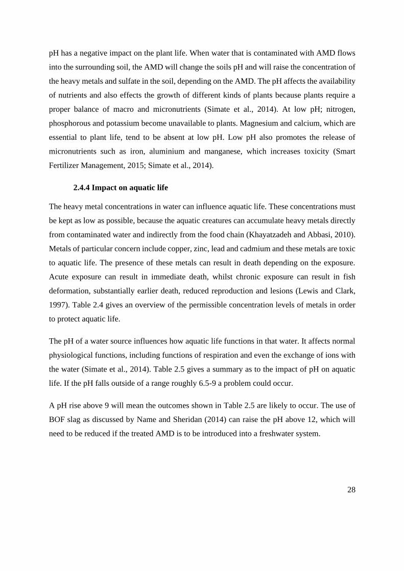
1997). Table 2.4 gives an overview of the permissible concentration levels of metals in order

to protect aquatic life.

The pH of a water source influences how aquatic life functions in that water. It affects normal

physiological functions, including functions of respiration and even the exchange of ions with

the water (Simate et al., 2014). Table 2.5 gives a summary as to the impact of pH on aquatic

life. If the pH falls outside of a range roughly 6.5-9 a problem could occur.

A pH rise above 9 will mean the outcomes shown in Table 2.5 are likely to occur. The use of

BOF slag as discussed by Name and Sheridan (2014) can raise the pH above 12, which will

need to be reduced if the treated AMD is to be introduced into a freshwater system.

29

Table 2.4: Permissible levels of heavy metals concerning protection of aquatic life

(Solomon, 2008)

Heavy metal Permissible level according to the Canadian

water quality standards (ppb)

Aluminium 5 if pH < 6.5, 100 if pH > 6.5

Arsenic 5 (FW), 12.5 (SW)

Cadmium 0.017 (FW), 0.12 (SW)

Lead 1–7 Depending on water hardness, (amount

of calcium and magnesium salts in water)

Nickel 25–150 Depending on water hardness

Manganese None

Mercury 0.1

Zinc 30 FW

Chromium 𝐶𝑟6+: 1 (FW), 1.5 (SW); 𝐶𝑟3+: 8.9 (FW),

56 (SW)

Copper 2–4 Depending on water hardness (amount

of calcium and magnesium salts in water)

Selenium 1

FW - Fresh water, SW - Salt water, ppb - parts per billion

The prevention of AMD formation at the source is not economically feasible according to

Johnson and Hallberg (2005) and as such AMD remediation must be done in order to assure

these risks to human, plant and aquatic life can be reduced. Most treatment options are also

expensive and as such, innovative and less expensive solutions must be considered.

30

Table 2.5: Impact of PH on aquatic life (Thoreau, 2002)

PH Impact

3.0-3.5 Toxic to most fish; some plants and invertebrates can survive such

as the water bug, water boatmen and white mosses

3.5-4.0 Lethal to salmonids

4.0-4.5 Harmful to salmonids, tench, bream, roach, goldfish and the

common carp; all stock of fish disappear because embryos fail to

mature at this level

4.5-5.0 Harmful to salmonid eggs, fry and the common carp; the lake is

usually considered dead and a “wet desert”; it is unable to support a

variety of life

5.0-6.0 Critical pH level, when the ecology of the lake changes greatly. A

reduction of green plants occurs. The reduction in green plants

allows light to penetrate further so acid lakes seem crystal clear and

blue; snails and phytoplankton disappear

6.5-9.0 Harmless to most fish

9.0-9.5 Harmful to salmonids, harmful to perch if persistent

9.5-10.0 Slowly lethal to salmonids

10.5-11.0 Lethal to salmonids, carp, tench, goldfish and pike

11.0-11.5 Lethal to all fish

2.5 Review of acid mine drainage remediation options

The choice of remedial strategy and the extent of remediation should be guided by end use,

rather than by applying strict drinking water codes (as shown in Table 2.8). Should the AMD

be used as process plant water, it will not have to conform to any standards other than what the

plant requires. If the water is to be discharged to the environment, then the National Water Act

would apply or the City of Johannesburg, 2008 Metropolitan Municipality Water Services By-

laws, depending on where the treated AMD is discharged. If drinking water was the ultimate

goal, then the SANS codes would guide the extent of remediation. Thus, it is important to

define what remediation is deemed successful (or sufficient) in terms of this project and in

31

terms of the ultimate end use of the remediated AMD. Sufficient remediation in terms of this

experiment, as defined in the introduction, is to remediate AMD to crop irrigation limits

according to Table 2.8, however it is always important to asses source of the AMD and keep

in mind the use of the treated AMD.

AMD remediation is generally divided into three broad categories: active, passive and a

combination of the two. Johnson and Hallberg (2005) argue that a more useful division between

the remediation technologies are those that use biological activities and those that do not. These

biological or abiotic systems may then be further divided into active (requiring a continuous

input of resources to sustain the process, such as lime addition for abiotic) and passive (very

little resource required once put into action, such as aerobic wetlands for biological) (Johnson

and Hallberg, 2005; Johnson and Hallberg, 2002). A broader view of the sections and

subsection involving AMD remediation may be seen in Figure 2.2.

Figure 2.2: Remediation techniques for AMD (Johnson and Hallberg, 2002)

2.5.1 Prevention

Whilst treatment of AMD is economically the preferred practice at the moment according to

Johnson and Hallberg (2005), there are other methods to address AMD, which is to stop AMD

at the source. Oxygen and water are two of the three requirements for the formation of AMD,

32

without oxygen and water, AMD would not be a problem. From this statement two possible

outcomes become clear, prevent oxygen form reaching the sulfide rich minerals or prevent

water from interacting with these minerals. Johnson and Hallberg (2005) subsequently argue

the best but not the most economically feasible prevention of AMD is to seal underground

mines, as well as sealing all subsequent potential AMD producing materials. Further techniques

of AMD prevention and minimization are given in Figure 2.3. These prevention techniques

will adequately protect the sulfide rich minerals from contact with oxygen and water, thus

reducing AMD formation.

Figure 2.3: AMD formation minimization and prevention techniques (Johnson and

Hallberg, 2002)

Akcil and Koldas (2006) propose three main stages for the prevention, minimization or

remediation of AMD:

1. Primary control – control of acid generation

33

2. Secondary control – control of acid migration

3. Tertiary control – the collection effluent for treatment

Primary control focuses on predicting the potential for an ore body to generate AMD, but each

site has its own specific nuances and assessing each site can be costly (US EPA, 1994). Primary

control would involve stopping the formation of AMD, for instance not allowing the sulfide

materials to be exposed to oxygen, which essentially would require no mining activity to

happen. As discussed by Johnson and Hallberg (2002) this is not feasible.

Akcil and Koldas (2006) also stated that secondary control is unfeasible. Secondary factors act

to control the AMD that has been formed, such as not allowing the AMD to enter streams or

lakes; however, this again is not economically feasible (US EPA, 1994).

The generation of AMD is realistically unavoidable, and if it is not possible to prevent

generation, ultimately treatment will be required to mitigate the impact of AMD.

2.5.2 Active treatment

An active treatment process according to Johnson and Hallberg (2005) will require the

continuous input of resources to be sustained. Active treatments generally involve addition of

an alkaline chemical such as limestone, lime, caustic soda or ammonia (Gaikwad and Gupta,

2008; Ochieng et al., 2010). Active treatments aim to increase the pH and precipitate metals,

but can be costly (Jennings et al., 2008). Examples of some of the materials used in the active

treatment of AMD are found in Table 2.6.

The addition of an alkaline material will raise the pH, increase the rate of chemical oxidation

of ferrous iron (active aeration and hydrogen peroxide or a chemical oxidising agent must also

be implemented) and cause many of the dissolved metals to precipitate as hydroxides and

carbonates. The addition of alkaline or a chemical neutralising agent is the most common

practice applied in the treatment of AMD (Johnson et al., 2005; Whitehead et al., 2005) of these

lime, carbon neutralization and ion exchange are the most commonly used conventional

methods to treat AMD (Johnson et al., 2005; Taylor et al., 2005).

34

Table 2.6: Neutralisation materials that can be used for the treatment of AMD (Taylor

et al., 2005)

Materials used for neutralisation

Limestone (CaC𝑂3) Sodium carbonate (N𝑎2C𝑂3)

Quicklime (CaO) Sodium hydroxide (NaOH)

Hydrated lime (Ca(OH)2) Hydroxyapatite C𝑎5(P𝑂4)3(OH)2

Dolomite (CaMg(C𝑂3)2) Ammonia (N𝐻3)

Magnesite (MgC𝑂3) Potassium hydroxide (KOH)

Caustic magnesia (MgO) and/or Mg(OH)2 Calcium peroxide (Ca𝑂2)

Lime kiln dust (CaO, CaC𝑂3) Cement kiln dust (CaO, CaC𝑂3)

Fly-ash (Ca, Mg, Na and K oxides and

hydroxides)

Barium carbonate (BaC𝑂3)

Fluidized bed ash (Ca, Mg, Na and K

oxides and hydroxides)

Barium hydroxide (Ba(OH)2)

35

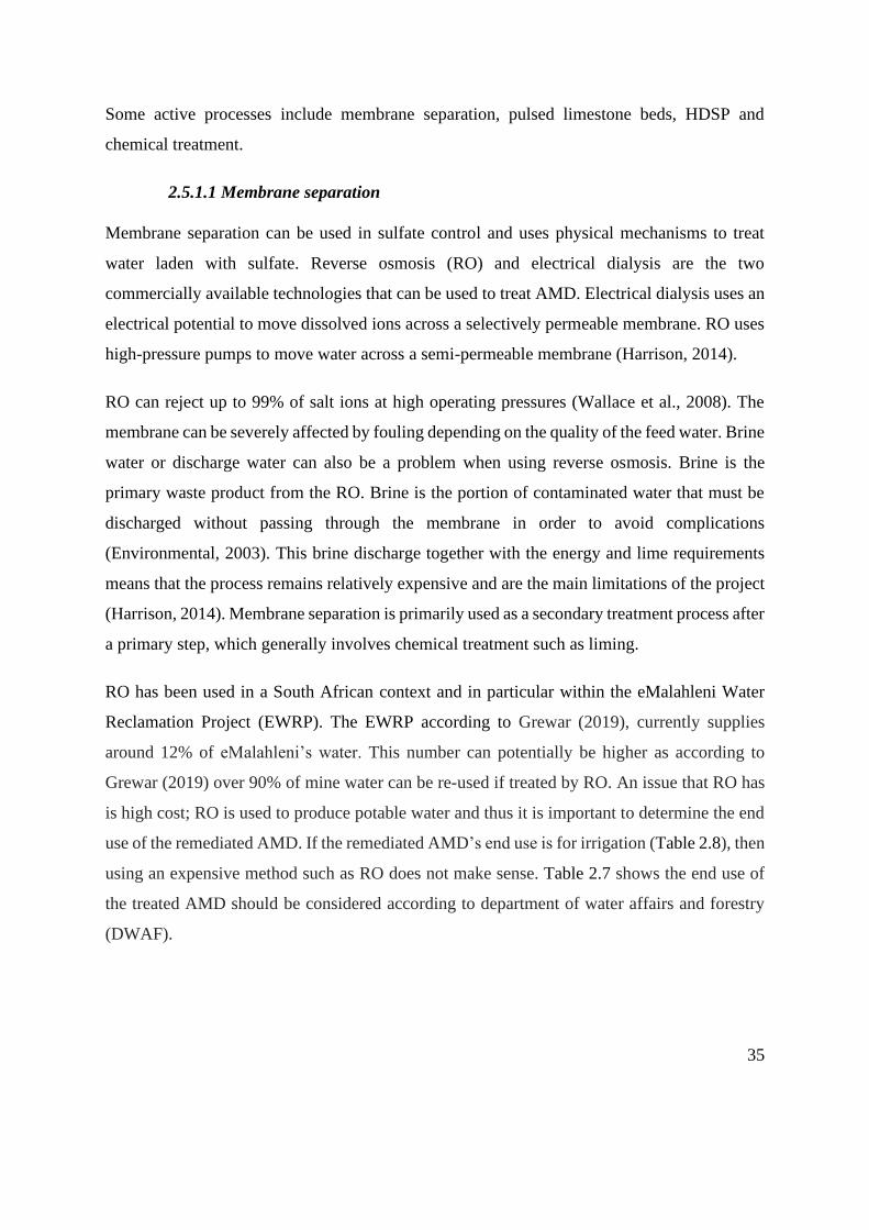
Some active processes include membrane separation, pulsed limestone beds, HDSP and

chemical treatment.

2.5.1.1 Membrane separation

Membrane separation can be used in sulfate control and uses physical mechanisms to treat

water laden with sulfate. Reverse osmosis (RO) and electrical dialysis are the two

commercially available technologies that can be used to treat AMD. Electrical dialysis uses an

electrical potential to move dissolved ions across a selectively permeable membrane. RO uses

high-pressure pumps to move water across a semi-permeable membrane (Harrison, 2014).

RO can reject up to 99% of salt ions at high operating pressures (Wallace et al., 2008). The

membrane can be severely affected by fouling depending on the quality of the feed water. Brine

water or discharge water can also be a problem when using reverse osmosis. Brine is the

primary waste product from the RO. Brine is the portion of contaminated water that must be

discharged without passing through the membrane in order to avoid complications

(Environmental, 2003). This brine discharge together with the energy and lime requirements

means that the process remains relatively expensive and are the main limitations of the project

(Harrison, 2014). Membrane separation is primarily used as a secondary treatment process after

a primary step, which generally involves chemical treatment such as liming.

RO has been used in a South African context and in particular within the eMalahleni Water

Reclamation Project (EWRP). The EWRP according to Grewar (2019), currently supplies

around 12% of eMalahleni’s water. This number can potentially be higher as according to

Grewar (2019) over 90% of mine water can be re-used if treated by RO. An issue that RO has

is high cost; RO is used to produce potable water and thus it is important to determine the end

use of the remediated AMD. If the remediated AMD’s end use is for irrigation (Table 2.8), then

using an expensive method such as RO does not make sense. Table 2.7 shows the end use of

the treated AMD should be considered according to department of water affairs and forestry

(DWAF).

36

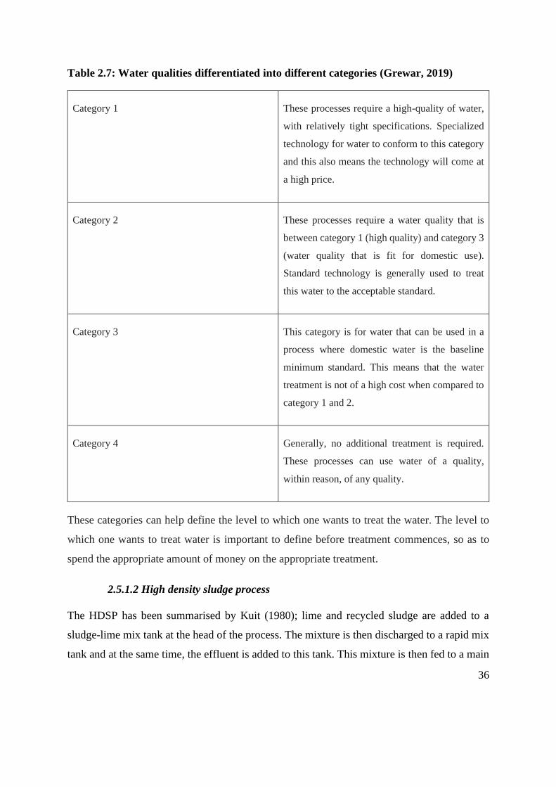
Table 2.7: Water qualities differentiated into different categories (Grewar, 2019)

Category 1 These processes require a high-quality of water,

with relatively tight specifications. Specialized

technology for water to conform to this category

and this also means the technology will come at

a high price.

Category 2 These processes require a water quality that is

between category 1 (high quality) and category 3

(water quality that is fit for domestic use).

Standard technology is generally used to treat

this water to the acceptable standard.

Category 3 This category is for water that can be used in a

process where domestic water is the baseline

minimum standard. This means that the water

treatment is not of a high cost when compared to

category 1 and 2.

Category 4 Generally, no additional treatment is required.

These processes can use water of a quality,

within reason, of any quality.

These categories can help define the level to which one wants to treat the water. The level to

which one wants to treat water is important to define before treatment commences, so as to

spend the appropriate amount of money on the appropriate treatment.

2.5.1.2 High density sludge process

The HDSP has been summarised by Kuit (1980); lime and recycled sludge are added to a

sludge-lime mix tank at the head of the process. The mixture is then discharged to a rapid mix

tank and at the same time, the effluent is added to this tank. This mixture is then fed to a main

37

lime reactor where a combination of aeration and high shear agitation are performed on the

mixture. This aids the process chemistry and clarifier performance. A flocculent is then added

and the mixture is sent to a flocculation tank, followed by a clarifier, which separates the treated

effluent from the sludge. A portion of the sludge is recycled to the head of the process.

The HDSP process is costly to build and operate. It can be a relatively complex process and its

performance will depend on the sludge recycle from the effluent, which sometimes needs a

thickener style clarifier (Kuit, 1980; Suvio, 2010; Mackie and Walsh, 2015).

South Africa has according to Grewar (2019) at least three HDSP plants in Krugersdorp,

Germiston and springs. These plants are able to treat water to the permissible limits (excluding

sulfate) to which water may be discharge according to Zhuwakinyu (2017) and can treat as

much as 50 ML/d, 82 ML/d, and 110 ML/d, per plant respectively. The permissible levels may

be seen in Table 2.8. The major problem with treating AMD using the HDSP process according

to Grewar (2019) is that the sulfate levels will not be reduced to the permissible levels when

treating a source with high levels of sulfate, in addition there are issues surrounding storage

and disposal of sludge waste.

2.5.1.3 pH Neutralisation Reagents

The most commonly used chemical treatment method is the addition of a reagent that raises

the pH, together with an aeration step to increase ferric iron chemical oxidation. The most

common reagents used are dolomite, lime, calcium carbonate, sodium carbonate or sodium

hydroxide. Due to economic reasons, the preferred reagents according to Johnson and Hallberg

(2005) are lime or calcium oxide. Liming as a treatment process can be effective in the removal

of sulfate as gypsum, as well as heavy metals through precipitation (Harrison, 2014).

Lime treatment involves bringing the pH of the AMD to a point where the metals of concern

become insoluble (Aubé and Zinck, 2003). Liming also removes sulfate to the saturation level

of gypsum (𝐶𝑎𝑆𝑂4. 2𝐻2𝑂), and dissolved heavy metals as metal hydroxides and oxides

(Harrison, 2014). A major disadvantage of liming is the sludge that is produced. This sludge

can be toxic as it contains heavy metals that are found in the treated AMD and is relatively

expensive to treat according to Johnson and Hallberg (2005).

38

Masindi, (2017) discusses the use of lime in South Africa. AMD field samples were taken from

the Mpumalanga province, South Africa and was treated with a few different technologies one

of which involved the use of lime. The unit which Masindi refers to as unit 2 uses lime and

raised the pH of a source of AMD with pH of 2 to 11 and almost halved the sulfate (30000 to

19000).

Advantages of active treatments:

● A smaller area is required for active treatments; generally, passive treatments such as

wetlands require large areas.

● They can cope with higher quantities of water contaminated with AMD.

Disadvantages of active treatments:

● Active systems are generally associated with high operating costs.

● Constant monitoring and maintenance are required; and the disposal of the sludge

produced provides yet another dilemma. According to Ochieng et al. (2010), the

active treatment route does not appear to be a long-term solution.

● The sludge produced is difficult to dispose of or expensive to treat.

2.5.3 Passive remediation technique

Passive treatment of AMD has been researched as an alternative approach to the generally

costlier active treatment methods (Johnson et al., 2005; Taylor et al., 2005). Passive treatment

has the ability to treat AMD, with a lower cost and has a less vigorous maintenance and

monitoring regime, thus according to Name (2013) and Ochieng et al. (2010) passive treatment

is arguably the best option for future treatment of AMD, however this must be caveated with

the knowledge that passive treatment is limited especially in terms of flowrate.

Some passive processes include: CW, PRB

2.5.2.1 Constructed Wetlands

CW’s have been used for centuries, as a treatment method to remediate AMD. In general, CW’s

are engineered pieces of land, which have constructed vegetation, which contains organisms

that treat water; it also provides a filtration mechanism made from soil, in which the vegetation

grows. Wetlands can be separated into two categories: anaerobic and aerobic wetlands. Aerobic

39

wetlands contain vegetation planted in relatively impermeable sediments such as clay, with

wetland vegetation characterized by horizontal flow of water (Taylor et al., 2005). Aerobic

wetlands are classified as shallow water bodies, which provide enough retention time.

Anaerobic wetlands consist of organic matter generally as some form of animal waste, sawdust

or compost (Johnson and Hallberg, 2005), they are generally construed underground and built

with organic rich substrates.

2.5.2.2 Packed reactor bed

PRB’s are buried layers of active material (this is dependent on the user but normally comprises

a combination of materials such as organic matter and limestone). The organic matter will

promote SRB growth, which will result in hydrogen sulfide formation. A precipitate may also

form with some of the heavy metals found in the AMD (Taylor et al., 2005).

For the PRB to treat the AMD effectively the entering effluent must have a low oxygen

concentration when it meets the reactive barrier. PRB’s are ideally suited to low temperatures

(Taylor et al., 2005).

Advantages of passive remediation:

● Considered self-sufficient and do not require human monitoring;

● Extremely cost efficient; and

● Can generally be used for several years.

Disadvantages of passive treatment:

● In general, cannot endure when the flow rate is high;

● Require large areas in comparison to active systems; and

● Treatment residence time can be long when compared to active systems.

2.5.4 Reducing and Alkalinity Producing Systems

This is a system, which essentially combines active and passive processes, normally with a

combination of organic matter and an alkaline reagent. The SRB’s will reduce sulfate by using

organic matter as previously discussed and the alkaline reagent will raise the pH which will

also precipitate out heavy metals to a level that SRB’s will not. In general RAPS (Taylor et al.,

2005):

40

● Utilize mixtures of limestone and organic matter, which can be used as a carbon

source for SRB;

● Rely on SRB to remove sulfate and on alkalinity generation via limestone dissolution;

● Provide sites for metal adsorption (the organic material); and

● Raise the pH of the water to near neutral conditions.

RAPS have disadvantages such as constant maintenance, high capital costs and RAPS tend to

be subject to clogging with gypsum and metal precipitates (Taylor et al., 2005).

In this study, a RAPS process using a combination of chemical and passive treatment is

proposed. SCB and BOF slag is utilized in this process. The SCB and BOF slag applications

are discussed in the sections to follow.

2.6 Water codes and restrictions in the South African context

2.6.1 Standards and restrictions

The treatment of AMD should be done with the end use of the remediated AMD in mind. If

the end use of the treatment is to produce water that will be drunk by South Africans, then the

South African national standard (SANS 241:2015) would be a minimum restriction. If the

treated AMD is to be discharged into a water source in the environment, then the National

Water Act would apply or the City of Johannesburg, 2008 Metropolitan Municipality Water

Services By-laws. The chosen location of discharge permissible limits and the permissible

limits for SANS 241:2015 for some heavy metals, sulfate and pH are shown in Table 2.8. If

the end goal for the treated AMD is that it is to be used in the plant then the plant engineer will

govern the treatment of the AMD and the engineer will govern the permissible levels of pH,

sulfate and heavy metals.

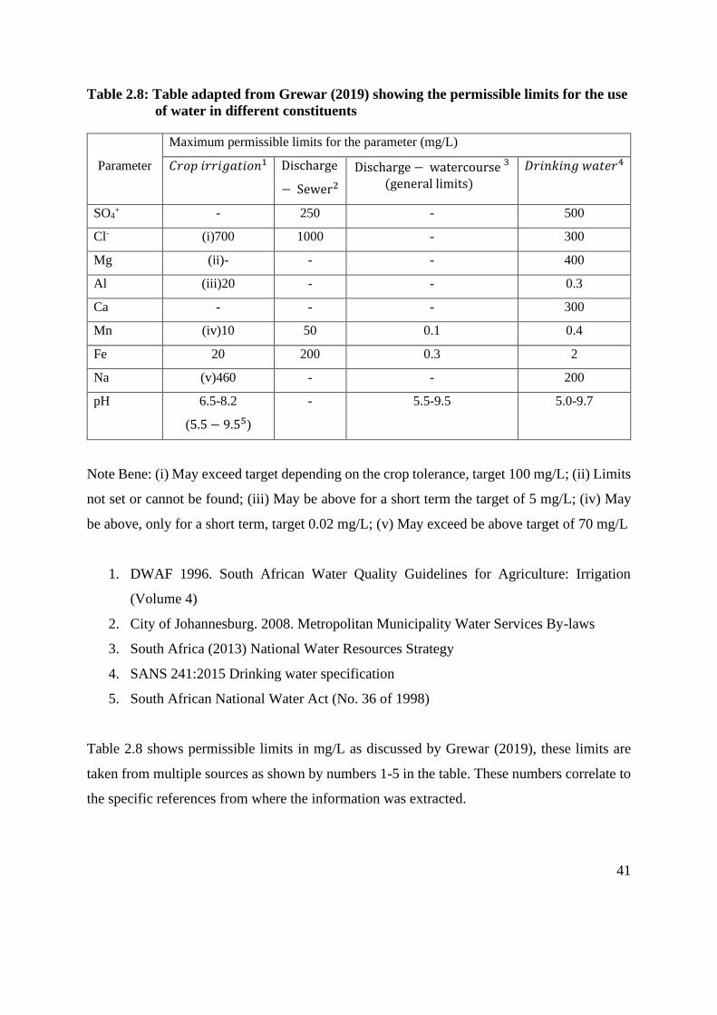
41

Table 2.8: Table adapted from Grewar (2019) showing the permissible limits for the use

of water in different constituents

Parameter

Maximum permissible limits for the parameter (mg/L)

𝐶𝑟𝑜𝑝 𝑖𝑟𝑟𝑖𝑔𝑎𝑡𝑖𝑜𝑛1 Discharge

− Sewer2

Discharge − watercourse (general limits)

3

𝐷𝑟𝑖𝑛𝑘𝑖𝑛𝑔 𝑤𝑎𝑡𝑒𝑟4

SO4+ - 250 - 500

Cl- (i)700 1000 - 300

Mg (ii)- - - 400

Al (iii)20 - - 0.3

Ca - - - 300

Mn (iv)10 50 0.1 0.4

Fe 20 200 0.3 2

Na (v)460 - - 200

pH 6.5-8.2

(5.5 − 9.55)

- 5.5-9.5 5.0-9.7

Note Bene: (i) May exceed target depending on the crop tolerance, target 100 mg/L; (ii) Limits

not set or cannot be found; (iii) May be above for a short term the target of 5 mg/L; (iv) May

be above, only for a short term, target 0.02 mg/L; (v) May exceed be above target of 70 mg/L

1. DWAF 1996. South African Water Quality Guidelines for Agriculture: Irrigation

(Volume 4)

2. City of Johannesburg. 2008. Metropolitan Municipality Water Services By-laws

3. South Africa (2013) National Water Resources Strategy

4. SANS 241:2015 Drinking water specification

5. South African National Water Act (No. 36 of 1998)

Table 2.8 shows permissible limits in mg/L as discussed by Grewar (2019), these limits are

taken from multiple sources as shown by numbers 1-5 in the table. These numbers correlate to

the specific references from where the information was extracted.

42

2.6.2 Acid mine drainage impact on the Witbank environment

The extent of remediation of AMD will depend on the ultimate use of the treated AMD. Should

the AMD be used for drinking purposes the South African national standard (SANS) provides

the legislative requirements in terms of quality as seen in Table 2.8.The particular area of

concern that Mativenga et al. (2018) discusses is the upper Olifants River, which is the

catchment of Witbank Dam, in the jurisdiction of Emalahleni Local Municipality in South

Africa. The sample data discussed in Mativenga’s paper was all data gathered from water

authorities (i.e. the drinking water standards) from the respective region and from the

municipality. This data was compared to what SANS recommends for drinking water; Table

2.8 and then Table 2.9 was reconstructed and shows the data for the Witbank catchment dam.

Table 2.9: Table adapted from Mativenga (2018) showing specific parameters for an

area

Parameter ELM Witbank dam raw

water

DWS catchment

pH 7.29 7.77

Sulfate in (mg/L) 152.24 314.30

Manganese in

(mg/L)

4.02 0.37

Iron (mg/L) N/A N/A

As shown in Table 2.8, the permissible limits for drinking water in South Africa show that any

water with a pH below 5 is outside of the limits. Whilst this was not relevant to Mativenga et

al. (2018) in terms of being outside of the limits, it is relevant to most other AMD sources,

which will present as a low pH (Foudhaili et al., 2019). A parameter that is not discussed by

Mativenga et al. (2018), but a parameter that is relevant to most AMD sources is iron, which

according to SANS (2015) should not be over 2 mg/L for drinkable water.

2.7 Overview of Sugar cane bagasse

SCB is a by-product of the crushing of sugar cane in the production of sugar. SCB is among

the most abundant lignocellulosic substances in South Africa and is a renewable feedstock

often used for power generation (Anukam et al., 2013). Cerqueira et al. (2007) gives the

common production of SCB; where 1 ton of Sugar cane produces 280kg of SCB, and

43

throughout the world about 54 million dry tons of SCB are produced annually (Anukam et al.,

2013), while in South Africa 6 million tons of raw SCB are produced annually according to

Anukam et al. (2013). The typical composition of SCB found in South Africa is given in Table

2.10.

Table 2.10: Typical chemical composition (wt.%) of extractive free sugar cane bagasse

found in South Africa (Alves et al., 2010)

Typical composition of sugar cane bagasse in South Africa according to Alves et al. (2010)

% Glucan 41.4 ± 0.4a

% Xylan 23.9 ± 0.2a

% Galactan 0.6

% Mannan 0

% Arabinan 2.4

% Lignin 23.9 ± 0.3a

% Acetyl 2.8

% 𝑈𝑟𝑜𝑛𝑖𝑐𝑠𝑏 1.2c

%Me-GluU 0.8c

% Ash 2.1

% Total 99.1

a Average for 2–4 samples plus estimated 95% confidence interval.

b Glucuronic and galacturonic acids.

c Methanolysis value; calculated as anhydrides.

This table shows the source of the carbohydrates for a typical South African SCB. This can

give some indication as to the composition of the SCB used in this study.

Grubb et al. (2018) have studied the implementation of a sulfate removal system that utilizes

SCB as the carbon source and the SRB go through the DSR cycle to convert sulfate to sulfide.

The work notes the material and conditions that the authors used to set up this microbially–

mediated environment. The study used AMD from Peruvian mine tailings to generate AMD

solutions for microcosm experiments and the results indicated that SCB was sufficient for metal

44

removal. The flow through experiments used AMD solutions with a pH of 3 that came from a

mine portal and the columns were packed with American SCB.

The Peruvian SCB was placed in AMD solutions with liquid: solid ratios of 5:10 and 20:1. The

following testing systems were used, bagasse only, bagasse with 0.1g glucose, bagasse seeded

with 5 mL of municipal digester sludge (DS) and bagasse with glucose and DS (Grubb et al.,

2018).

The results for the microcosm experiments indicate that the columns inoculated with DS were

effective in significant removal of heavy metal concentrations, namely arsenic which in 90

days had a removal percent of close to 90; the columns not inoculated were not effective in

heavy metal reduction with the exception of lead. The results indicated that the SCB inoculated

with DS was the most effective way in which to achieve a remediation method for a relatively

low pH AMD. The metal reduction in the DS inoculated columns was observed to achieve

significant results within a 90-day period. Grubb et al. (2018) also discuss the pH changes

within the system and established that the DS columns were the most effective at raising the

pH of the system to circumneutral values depending on the AMD: Solid ratios.

For the flow through studies, the sulfide generation within the DS column was effective and

according to Grubb et al. (2018), was more effective than the other columns not inoculated

with DS. It was also evident from the results that temperature influenced metal precipitation

and sulfide production. The columns were also effective at reducing metal concentrates and

buffering pH towards neutral conditions.

2.8 Overview of Sulfate reducing bacteria and their use

Bioreactors are essentially vessels in which biological reactions occur as demonstrated by

Ramla and Sheridan (2015) who used beakers for their reactors. Their bioreactors contained

organic material, in which SRB are able to use the organic material as a carbon source when

using sulfate to convert into sulfide (Ramla and Sheridan, 2015). Sulfate reducing bioreactors

have received a lot of attention for their ability to treat AMD and the carbon source has been

of particular interest (Zagury and Neculita, 2007). The SRB must ultimately use dissimilatory

45

sulfate reduction (DSR) to convert the sulfate into sulfide and the most important part of the

bioreactor is this process.

SRB have the capability of using sulfate and through DSR, which can convert the sulfate into

sulfide, which in turn reacts with metals to form metal sulfide precipitates (Taylor, 2005). SCB

can be a host media for the SRB as it is a source for simple organic carbon; its insoluble

remaining carbohydrates are able to slowly hydrolyse under acidic conditions into bioavailable

oligosaccharides (Grubb et al., 2018).

Biological DSR is heavily reliant on the presence of complementary microorganisms; these

microorganisms must be able to coexist within the reaction vessel and will form an ecosystem.

This ecosystem will then release volatile fatty acids (VFA’s), which are important, as most

SRB are heterotrophic (Harrison, 2014). SRB will be the main microorganisms responsible for

DSR, however other microorganisms present in the system will assist directly with sulfate

reduction, or indirectly by generating more nutrients for the SRB. Acidogenic bacteria are one

type of microorganism that will assist with the DSR mechanism, through acidogenesis (a

process that takes sugars and complex carbohydrates and converts them into VFA’s through

fermentation) (Alexiou and Panter, 2004; Dauknys et al. 2017). This whole process allows the

SRB to reduce sulfate to sulfide along with bicarbonate, which will raise pH, as shown in

Equation 2.6 according to Kaksonen and Sahinkaya (2012), this process is done through DSR,

in which an electron donor is used, as is a carbon source; the carbon source in this experiment

will be SCB.

𝑆𝑂42− + 2𝐶𝐻2𝑂 → 𝐻2𝑆 + 2𝐻𝐶𝑂3 (2.6)

The hydrogen sulfide then has the ability to form insoluble precipitates as shown in Equation

2.7 (Taylor, 2005).

𝐻2𝑆 + 𝑀2+ → 𝑀𝑆 + 2𝐻+ (2.7)

This allows for the precipitation of heavy metals at suitable pH values in relation to the SRB.

The effectiveness of the sulfate removal in terms of SRB acclimation will depend on the pH

46

value, population size of the SRB, the presence of acidogenic bacteria, temperature and any

potential exposure to air (Zhang et al., 2013).

2.8.1 Sulfur and iron oxidizing microorganisms

Microorganisms can be used in a large tank aeration process for a commercial extraction of a

variety of metals including (copper, cobalt and gold) (Rawlings, 2005). Some characteristics

according to Rawlings (2005) of the microorganisms is their ability to grow autotrophically,

their acid-tolerance and their metal resistance. Growing a specific genus of microorganism is

very hard because bio-mining organisms will occur in a consortium, which will mean that

there will be cross contamination of some organisms that are not required (Rawlings, 2005).

What is important to do with any introduction of a consortium of organisms to a new

environment is to make the conditions of the environment suitable to the organisms, which

you most desire in the particular environment. Thus, for an environment, considering SRB, it

is known that a pH value of 5.5-7.5 or 4.5-7.5 is ideal depending on the genus of the SRB

according to Zhang et al. (2013).

Aguinaga et al. (2019) studied the activities that sulfur and iron oxidizing bacteria have in

releasing alkalinity. These bacteria according to Aguinaga et al. (2019) are able to release this

alkalinity through chemical reactions. In the presence of organic matter and with a depleted

oxygenated environment combined with bacteria the reducing conditions will change the

speciation and distribution of metals within a wetland (Aguinaga et al., 2019). According to

Aguinaga et al. (2019), Epel et al. (2005) and Muyzer and Stams, (2008), there are specific

genes related to sulfur oxidation and reduction which include soxB, which encodes a protein

essential for thiosulfate bacterial oxidation and subsequent sulfur oxidation and the dsrA

gene, which encodes a sulfite reductase responsible for dissimilatory sulfate reduction. This is

not as clear when considering iron oxidation and reduction (Aguinaga et al., 2019).

2.9 Overview of basic oxygen furnace slags and the application of basic

oxygen furnace slag in acid mine drainage remediation

Slags are by-products of the metallurgical process. One process, which is used to make metal

is known as the BOF process, which uses lime (calcium oxide) as a flux. BOF slags are highly

47

alkaline. This is due to their composition, which primarily has hydrated amorphous silica,

calcium oxide and magnesium oxide (Ziemkiewicz and Skousen, 1988). BOF slag is formed

during the conversion of hot metal from the blast furnace into steel in a basic oxygen furnace.

When the reaction is complete, liquid molten steel collects at the bottom of the furnace while

the liquid slag floats on top. The liquid steel and slag are then tapped into separate pots at high

temperatures. The liquid slag can then be treated by the addition of silicon dioxide and oxygen

in order to increase volume stability. It is then then poured into pits where the slag is air cooled

under controlled conditions, to form crystalline slag (Euroslag, 2017). There is a wide range of

applications for BOF slags and AMD remediation does not need to compete with some of these

applications for the BOF slag material, as the leaching of the lime from the BOF slags can help

with volume stability in road construction, which is a problem addressed by Reddy et al.

(2006).

Slags have a wide range of applications such as road construction, cement production and even

landfill. This material is used often in niche civil engineering works (Ziemkiewicz and

Skousen, 1988). The use of BOF slag in civil construction and road ballast is well known. The

presence of free high lime in the slag results in swelling (Reddy et al., 2006). This swelling

from the high concentration of free lime can potentially be removed by use of the slag in AMD

remediation. BOF slag is referred to as ferrous slag, where slag is generally divided into 3

categories, the ferrous smelting process slag category denotes slags that contain less iron than

non-ferrous smelting slag. BOF slag is mainly comprised of CaO, Fe, 𝐴𝑙2𝑂3, MgO and 𝑆𝑖𝑂2

(Shen and Forssberg, 2003). This composition makes the slag a potentially able alkaline

material, to use for AMD remediation in a low pH AMD source.

Many authors describe the potential use of slag as a relatively low-cost neutralization agent

(Ziemkiewicz and Skousen, 1988; Ziemkiewicz et al., 2003; Shen and Forssberg, 2003; Name

and Sheridan, 2014; Name, 2013; Sheng et al., 2014). The use of slag as a remediation tool for

AMD, has grown because the current routes are not viewed as long term solutions due to high

cost and even difficulties with the technologies, such as potential sludge disposal problems

(Johnson and Hallberg, 2005). The use of Slag in AMD remediation would create better

sustainability in mining, as the slag used would be a secondary mining related by-product of

the mining process and reusing the slag to treat AMD is a sustainable process. The BOF slag

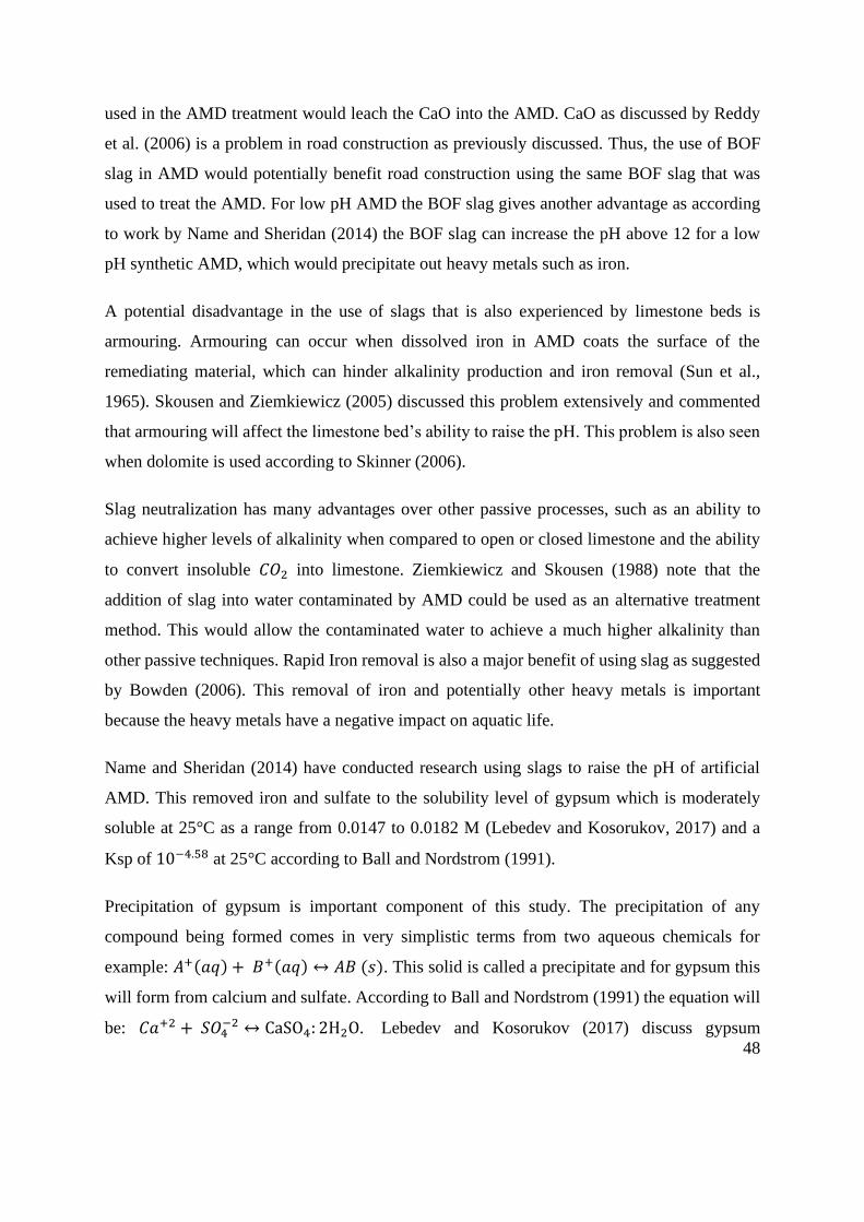
48

used in the AMD treatment would leach the CaO into the AMD. CaO as discussed by Reddy

et al. (2006) is a problem in road construction as previously discussed. Thus, the use of BOF

slag in AMD would potentially benefit road construction using the same BOF slag that was

used to treat the AMD. For low pH AMD the BOF slag gives another advantage as according

to work by Name and Sheridan (2014) the BOF slag can increase the pH above 12 for a low

pH synthetic AMD, which would precipitate out heavy metals such as iron.

A potential disadvantage in the use of slags that is also experienced by limestone beds is

armouring. Armouring can occur when dissolved iron in AMD coats the surface of the

remediating material, which can hinder alkalinity production and iron removal (Sun et al.,

1965). Skousen and Ziemkiewicz (2005) discussed this problem extensively and commented

that armouring will affect the limestone bed’s ability to raise the pH. This problem is also seen

when dolomite is used according to Skinner (2006).

Slag neutralization has many advantages over other passive processes, such as an ability to

achieve higher levels of alkalinity when compared to open or closed limestone and the ability

to convert insoluble 𝐶𝑂2 into limestone. Ziemkiewicz and Skousen (1988) note that the

addition of slag into water contaminated by AMD could be used as an alternative treatment

method. This would allow the contaminated water to achieve a much higher alkalinity than

other passive techniques. Rapid Iron removal is also a major benefit of using slag as suggested

by Bowden (2006). This removal of iron and potentially other heavy metals is important

because the heavy metals have a negative impact on aquatic life.

Name and Sheridan (2014) have conducted research using slags to raise the pH of artificial

AMD. This removed iron and sulfate to the solubility level of gypsum which is moderately

soluble at 25°C as a range from 0.0147 to 0.0182 M (Lebedev and Kosorukov, 2017) and a

Ksp of 10−4.58 at 25°C according to Ball and Nordstrom (1991).

Precipitation of gypsum is important component of this study. The precipitation of any

compound being formed comes in very simplistic terms from two aqueous chemicals for

example: 𝐴+(𝑎𝑞) + 𝐵+(𝑎𝑞) ↔ 𝐴𝐵 (𝑠). This solid is called a precipitate and for gypsum this

will form from calcium and sulfate. According to Ball and Nordstrom (1991) the equation will

be: 𝐶𝑎+2 + 𝑆𝑂4−2 ↔ CaSO4: 2H2O. Lebedev and Kosorukov (2017) discuss gypsum

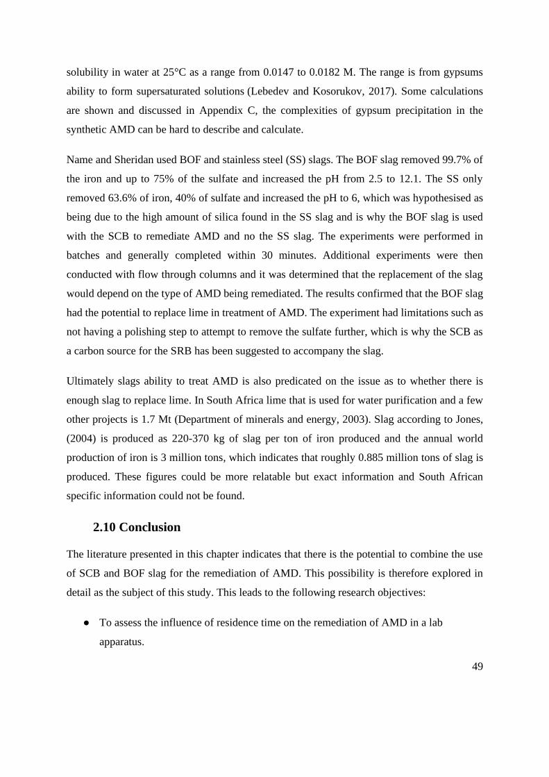
49

solubility in water at 25°C as a range from 0.0147 to 0.0182 M. The range is from gypsums

ability to form supersaturated solutions (Lebedev and Kosorukov, 2017). Some calculations

are shown and discussed in Appendix C, the complexities of gypsum precipitation in the

synthetic AMD can be hard to describe and calculate.

Name and Sheridan used BOF and stainless steel (SS) slags. The BOF slag removed 99.7% of

the iron and up to 75% of the sulfate and increased the pH from 2.5 to 12.1. The SS only

removed 63.6% of iron, 40% of sulfate and increased the pH to 6, which was hypothesised as

being due to the high amount of silica found in the SS slag and is why the BOF slag is used

with the SCB to remediate AMD and no the SS slag. The experiments were performed in

batches and generally completed within 30 minutes. Additional experiments were then

conducted with flow through columns and it was determined that the replacement of the slag

would depend on the type of AMD being remediated. The results confirmed that the BOF slag

had the potential to replace lime in treatment of AMD. The experiment had limitations such as

not having a polishing step to attempt to remove the sulfate further, which is why the SCB as

a carbon source for the SRB has been suggested to accompany the slag.

Ultimately slags ability to treat AMD is also predicated on the issue as to whether there is

enough slag to replace lime. In South Africa lime that is used for water purification and a few

other projects is 1.7 Mt (Department of minerals and energy, 2003). Slag according to Jones,

(2004) is produced as 220-370 kg of slag per ton of iron produced and the annual world

production of iron is 3 million tons, which indicates that roughly 0.885 million tons of slag is

produced. These figures could be more relatable but exact information and South African

specific information could not be found.

2.10 Conclusion

The literature presented in this chapter indicates that there is the potential to combine the use

of SCB and BOF slag for the remediation of AMD. This possibility is therefore explored in

detail as the subject of this study. This leads to the following research objectives:

● To assess the influence of residence time on the remediation of AMD in a lab

apparatus.

50

● To understand breakthrough of a potential remediation system.

● To study the physical and chemical changes of BOF slag during remediation of the

AMD.

These objectives lead to the 4 different configurations, which were constructed in order to

address the objectives.

51

3 Experimental Material and Methods

3.1 Introduction

This study proposes the treatment of synthetic AMD with a combination of sugarcane bagasse

(SRB) and Basic oxygen furnace (BOF) slag. In order to address the research objectives as

given in Chapter 1, experiments were performed to treat synthetic AMD in different process

configurations using these two materials. A series of columns packed with either SRB or BOF

slag or a combination of the two were used in these studies. Details of the experimental setups

and procedures are given in the next sections.

3.2 Experimental

3.2.1 Description of experimental apparatus

Four different process configurations were built and tested to determine the most suitable

combination of BOF slag and SCB in the treatment of synthetic AMD. Each configuration

consisted of a series of columns connected to each other and a reservoir with flexible PVC

tubing (ID 3mm). The columns were made from hard PVC pipes with an OD of 40mm and

each column was 20cm in length. The packing materials (BOF slag or SCB) were kept in place

in the columns by an acrylic roof membrane, which allowed water to pass through but not the

remediating material. The configurations were set up for the synthetic AMD to be passed

vertically upwards through the columns from the AMD reservoir using a Watson-Marlow

peristaltic dosing pump. A photo of the setup is presented in Figure 3.1.

52

Figure 3.1: Photograph depicting the experimental set up in the lab

The middle column was a redundant experiment.

Configuration A (Figure 3.2) consisted of two sugar cane bagasse (SCB) columns in series,

followed by an aeration column. This configuration was similar to the one used in a previous

A

Configurations

B C D

53

study by Grubb and co-worker’s (2018). The aeration unit is set up to help oxidation of Fe (II)

to Fe (III).

Figure 3.2: Schematic of experimental apparatus for configuration A

Configuration B consisted of an SCB column followed by a BOF slag column and the aeration

column. The slag column was packed with slag particles smaller than 10mm in diameter. This

configuration was tested in response to the low pH observed in the outlet of configuration A as

mentioned in Grubb et al. (2018). The aeration unit is set up to help oxidation of Fe (II) to Fe

(III).

Figure 3.3: Schematic of experimental apparatus for configuration B

Configuration C (Figure 3.4) consisted of two columns in series packed with a combination of

SCB (30%) and BOF slag (70%) in each column. This configuration was used to determine if

54

a combination of the two substances would have any impact on the treatment of AMD. The

aeration unit is set up to help oxidation of Fe (II) to Fe (III).

Figure 3.4: Schematic of experimental apparatus for configuration C

The fourth configuration, configuration D (Figure 3.5), consisted of a BOF slag column

followed by a SCB column. This configuration was used to assess the influence of raising the

pH of the AMD first before passing it up through the SCB column. In this configuration the

SCB column would potentially act as the polishing step. The aeration unit is set up to help

oxidation of Fe (II) to Fe (III).

Figure 3.5: Schematic of experimental apparatus for configuration D

55

3.3 Materials

3.3.1 Sugar cane bagasse

The SCB was obtained from UCL Dalton located at 16 Noodsberg Road, Dalton, South Africa.

SCB of size 2.5-4cm was packed into the columns of the various configurations.

3.3.2 Basic oxygen furnace slag

BOF slag was obtained from Phoenix Slag Services. It was chosen over Stainless Steel slag,

as it has a lower silicon dioxide (SiO2) content, and silicon dioxide forms a glass type layer

over the slag (Name and Sheridan, 2014). This glass type layer does not allow as much contact

with the lime (CaO) and subsequently the slag with higher silicon dioxide content will not raise

the pH as high as the one with the lower SiO2 content. A BOF slag size of less than 10mm (0.2-

1cm) was sorted out by hand for use in the study.

3.3.3 Simulated acid mine drainage

The typical AMD found in a Witwatersrand gold basin according to Name and Sheridan (2014),

was simulated in a laboratory. The low pH and high levels of iron and sulfate concentration in

the simulated AMD are in line with some of the harsher AMD concentrations found in the

Witwatersrand basin. The synthetic AMD was formulated according to recommendations by

Potgieter-Vermaak (2006). The synthetic AMD’s sulfate level changed over the course of the

experiments but was kept in a range of 4300-6250 ppm, which according to Name and Sheridan

(2014) is considered a high strength AMD. The total iron content was kept in a range of 790-

1300 ppm and the pH was kept in a range of 2.3-3.4. The simulated AMD was made using

hydrated ferrous sulfate (𝐹𝑒𝑆𝑂4. 7𝐻2𝑂), deionised water, sulfuric acid and calcium carbonate.

The hydrated ferrous sulfate came from Protea chemicals, South Africa and assayed at 90%

pure. The deionised water was obtained from the University of Witwatersrand. The sulfuric

acid was retrieved from Merck, South Africa and assayed at 95-99% pure. The calcium

carbonate (analytical grade) was sourced from Associate Chemical Enterprises.

56

3.4 Experimental Procedure

3.4.1 Column packing and sulfate reducing bacteria pre-treatment

Before the assembly of the experimental configurations and the subsequent AMD treatment

studies, the columns were packed with the BOF slag and sugarcane bagasse. This was followed

by the inoculation of the sugarcane bagasse columns with sulfate reducing bacteria.

The bagasse only columns were packed with approximately 38.52 ± 0,1g of SCB. The columns

containing a mixture of SCB and BOF slag (configuration C) were packed with approximately

19.26± 0,1g of SCB and 175.05 ± 0,1g of BOF slag. The slag only columns were packed with

approximately 350.07 ± 0.1g of slag.

The SCB was inoculated with digester sludge sourced from the Olifantsvlei wastewater

treatment works. 12 mL of digester sludge was added to all the columns containing only SCB

and 6 mL was added to all the columns containing a mixture of SCB and BOF slag. The

columns were then sealed and left for 2 days to allow the bacteria in the column to grow before

exposure to AMD. Following the two days, all the columns were exposed to a solution

containing sulfuric acid of a concentration of 2000 ppm, deionised water and sodium hydroxide

(34.45g) with pH 6.67. This solution was passed through the system for 5 days before the

synthetic AMD was introduced. It allowed for acclimation of the sulfate reducing bacteria,

which promoted bacterial growth.

3.4.2 Acid mine drainage in different process configurations

In order to assess the performance of each of the configurations in the treatment of AMD, the

variation in certain process parameters were studied. Initially specific parameters such as pH,

sulfate and iron concentrations were tracked. In later experiments the calcium and sulfide

concentrations were also measured after careful consideration of the data from the earlier

experiments. The calcium and sulfide content were considered necessary parameters because

a calcium concentration drop will indicate depletion or armouring of the BOF slag, which will

also indicate the start of breakthrough of the BOF slag. The presence of sulfide will most likely

indicate hydrogen sulfide production, and a drop-in concentration would indicate the start of

breakthrough. Where breakthrough is defined as the sulfate or iron concentration in the inlet

57

(synthetic AMD feed) equalling the concentration in the outlet, it has also been defined as the

point at which the pH in the inlet (synthetic AMD feed) equals the pH in the outlet. The start

of breakthrough is defined as the point at which the pH drops in relation to the previous point.

The influence of operating conditions such as residence time was also investigated. The

residence time of AMD in the different process configurations were varied. An initial test was

performed where the residence time was approximately 12 h for each column. In these tests,

pH was used as a measure of when breakthrough started to occur. This was followed by

additional experiments at residence times of 35.5h ± 5.5 and 78.5h ± 7.5. The pH, iron and

sulfate concentrations were measured. Later calcium and sulfide content were also measured

for the low flow experiment (78.5h ± 7.5 residence time). Before the data from these parameters

was used the pore volume (PV) was calculated where PV was defined as the total volume of

water minus the volume of space the water takes up once the material is added over the total

volume of water and all of the columns were then considered together.

To understand breakthrough of a potential remediation system, the effects on the BOF slag as

one of the remediating substances was determined. The system’s decreased removal of iron or

sulfate, or a drop in the pH indicated the start of breakthrough. Studying the physical and

chemical changes of BOF slag during remediation of the AMD entailed an analysis of the BOF

slag both before and after treatment using a Carl Zeiss Sigma field emission scanning electron

microscope (SEM) equipped with an oxford EDX (energy dispersive X-ray) detector.

3.4.3 Sampling protocol

40 mL liquid samples were taken at each sample point until the point between the start of

breakthrough and when breakthrough occurred. The frequency of the sample taking was

dependent on the experiment that was being performed. For the high flow experiment, samples

were taken almost daily, and for the low flow experiments samples were taken approximately

every 2-3 days. From this 40 mL sample, a 5 mL aliquot was taken, filtered, and diluted to 15

mL with deionised water. 0.45 mL of Nitric acid was added to the 15 mL diluted sample

because this addition of nitric acid lowered the pH of that 15 mL sample to below 2, as

recommended by Environmental Protection Agency (1983). This allowed for the sample to be

stored and to be tested for iron at a later date using atomic absorption spectroscopy (AAS).

58

Another 5 mL sample was taken to measure total iron and total calcium for the low flow

experiments only, this sample was not filtered but was diluted with 10 mL of deionised water

and nitric acid was again added to be able to store the sample for analysis at a later date.

The remaining 30 mL was stored in a refrigerator at 2°C and was then analysed for sulfate

content using the barium chloride method as described in the analytical technique section,

Section 3.4.3.1. This was done within 3 weeks using a Merck SpectroQuant® Pharo 300 UV/VI

spectrophotometer.

Sulfide was also measured using the method described in Section 3.4.3.1; sulfide was measured

immediately after a small sample was taken directly from the sampling port.

Once enough data for the system had been gathered, the BOF slag in the system was taken out

and placed into separate airtight containers. The airtight containers were colour co-ordinated

to show which BOF slag was taken out of which specific configuration. The unused BOF slag

was put into a different airtight container. These samples were then taken for coating and

analysis as described in Section 3.4.3.1

3.4.3.1 Analytical techniques

In order to accurately determine the start breakthrough of the system, the composition of the

treated AMD had to have been known. The pH, sulfate, sulfide, iron and calcium were all

measured in the treated and untreated AMD. The used BOF slag was compared to the unused

BOF slag. The data was analysed using the built-in Excel function called ANOVA:

● Sulfide was measured using a Merck SpectroQuant® Pharo 300 UV/VIS set to a

wavelength of 670 nm. 0.2 mL zinc acetate was added to 4.8 mL of sample, which

was not diluted as the sample concentration of sulfide did not go over 3 ppm or under

0.02 ppm (as required). 0.5 mL of dimethyl-4-phenylenediamine was then added and

then 0.5 mL of ferric nitrate was added. The solution was left for 10 minutes exactly.

This solution was then measured in the Merck SpectroQuant® Pharo 300 UV/VIS

(Cline, 1969). The concentration was then calculated using a standard curve where

known concentrations of sulfide were measured using the same method described by

Cline (1969) and the absorbances of the samples were compared to this curve to get a

59

concentration of sulfide. To ensure consistency a sample of known concertation was

made. The absorbance was measured, and the concertation determined. If the

determined concertation was not within ±0.05 ppm of what was expected this was

noted and the reason as to why this had occurred was investigated and fixed before

the determination of the concentration of the rest of the samples.

● Sulfate was measured using a Merck SpectroQuant® Pharo 300 UV/VIS set to a

wavelength of 880 nm. 50𝜇𝑙 of glycerol was added to 5 mL of the diluted sample.

Barium Chloride was added after the 50𝜇𝑙 of glycerol, with a micro spoon directly

before shaking the vial; the vial was shaken for 10 seconds. Concentration was then

determined by comparison with a standard curve. The standard curve was made by

using the absorbance of known concentrations of sulfate. Three duplicate aliquots

(from the original sample) were taken to achieve consistent and reproducible data. As

it is sometimes hard with the Barium Chloride test to achieve consistency these

aliquots were compared with each other and if there was a difference of ±50 ppm

they were redone.

● The pH of all the samples and a sample of the synthetic AMD were measured using a

Metrohm 744 pH meter, within 25 minutes of sample collection. The calibration of

the pH meter was done with pH standards from Metrohm, with buffered solutions at a

pH = 4, 7 and 10. After every pH was measured the probe was immediately washed

with distilled water to prevent contamination of subsequent tests.

● Metallic ions were measured using an AAS. Gas mixtures of air and acetylene and

acetylene and nitrous oxide were used for iron and calcium respectively. The

detection wavelengths for each of the species are specified in the user manual.

● The samples of used and unused slag were scanned using a Carl Zeiss Sigma field

emission SEM equipped with an oxford EDX detector, using nitrogen as the gas. The

samples were first coated with carbon in accordance with Yamada et al. (1986),

before the chemical and physical properties on the surface of the BOF slag of the

sample were determined. The coating was done by the chemistry department at the

University of the Witwatersrand, the department used the spin coating method.

● ANOVA was used on the collected data to determine if there was any statistical

significance between the columns within the configuration and between the

60

configurations themselves. The ANOVA used was an in-built function in Excel, a

single factor ANOVA was used after consultation with Senior Lecturer David Rose at

the University of Witwatersrand.

61

4 Results

Synthetic AMD was treated in four process configurations comprising of different

combinations of BOF Slag and Sugarcane bagasse combinations to determine the best possible

combination for AMD treatment. In this study, the treatment of AMD implied a reduction in

sulphate and iron content and an increase in pH of the solution.

4.1 Characterization of slag

The BOF slag used in this experiment was obtained from SCAW metals located at Black Reef

Rd, Dinwiddie, Germiston, South Africa. It was analysed using XRF spectroscopy and the

report sent from phoenix services. The results are shown in Table 4.1: Composition of slag

measured by XRF spectroscopy through Phoenix Slag Services Newcastle South Africa, date:

16.11.2012-04.12.2012. The results concur with what had been found in literature where the

slag was primarily comprised of CaO, Fe, 𝐴𝑙2𝑂3, MgO and 𝑆𝑖𝑂2 according to Shen and

Forssberg (2003), it can also be seen in this compositional analysis that manganese was also a

relatively high percentage in the slag. The high CaO content was what caused the rise in pH,

in the AMD.

For this experiment the Proba 2, 9.55mm slag was used; this slag had relatively high levels of

CaO and was the slag that would be most readily available as was my understanding on

speaking to phoenix slags. Pictures of the BOF slag and SCB were taken before and after

treatment so that a visual analysis of the change could be seen and help confirm the results of

the EDX elemental surface analysis. The pictures are displayed in Figure 4.1, Figure 4.2 and

Figure 4.3, all the BOF slag and SCB that came out of the columns for each experiment looked

the same and thus only one picture was taken to confirm the visual change.

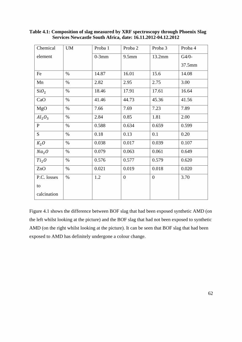
62

Table 4.1: Composition of slag measured by XRF spectroscopy through Phoenix Slag

Services Newcastle South Africa, date: 16.11.2012-04.12.2012

Chemical

element

UM Proba 1 Proba 2 Proba 3 Proba 4

0-3mm 9.5mm 13.2mm G4/0-

37.5mm

Fe % 14.87 16.01 15.6 14.08

Mn % 2.82 2.95 2.75 3.00

Si𝑂2 % 18.46 17.91 17.61 16.64

CaO % 41.46 44.73 45.36 41.56

MgO % 7.66 7.69 7.23 7.89

𝐴𝑙2𝑂3 % 2.84 0.85 1.81 2.00

P % 0.588 0.634 0.659 0.599

S % 0.18 0.13 0.1 0.20

𝐾2𝑂 % 0.038 0.017 0.039 0.107

𝑁𝑎2𝑂 % 0.079 0.063 0.061 0.649

𝑇𝑖2𝑂 % 0.576 0.577 0.579 0.620

ZnO % 0.021 0.019 0.018 0.020

P.C. losses

to

calcination

% 1.2 0 0 3.70

Figure 4.1 shows the difference between BOF slag that had been exposed synthetic AMD (on

the left whilst looking at the picture) and the BOF slag that had not been exposed to synthetic

AMD (on the right whilst looking at the picture). It can be seen that BOF slag that had been

exposed to AMD has definitely undergone a colour change.

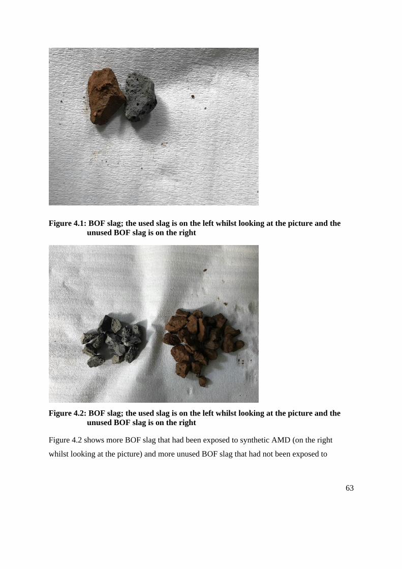
63

Figure 4.1: BOF slag; the used slag is on the left whilst looking at the picture and the

unused BOF slag is on the right

Figure 4.2: BOF slag; the used slag is on the left whilst looking at the picture and the

unused BOF slag is on the right

Figure 4.2 shows more BOF slag that had been exposed to synthetic AMD (on the right

whilst looking at the picture) and more unused BOF slag that had not been exposed to

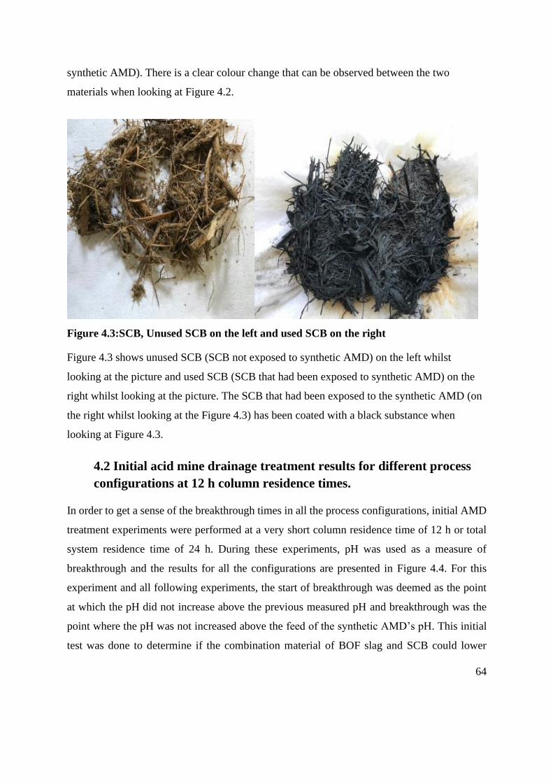
64

synthetic AMD). There is a clear colour change that can be observed between the two

materials when looking at Figure 4.2.

Figure 4.3:SCB, Unused SCB on the left and used SCB on the right

Figure 4.3 shows unused SCB (SCB not exposed to synthetic AMD) on the left whilst

looking at the picture and used SCB (SCB that had been exposed to synthetic AMD) on the

right whilst looking at the picture. The SCB that had been exposed to the synthetic AMD (on

the right whilst looking at the Figure 4.3) has been coated with a black substance when

looking at Figure 4.3.

4.2 Initial acid mine drainage treatment results for different process

configurations at 12 h column residence times.

In order to get a sense of the breakthrough times in all the process configurations, initial AMD

treatment experiments were performed at a very short column residence time of 12 h or total

system residence time of 24 h. During these experiments, pH was used as a measure of

breakthrough and the results for all the configurations are presented in Figure 4.4. For this

experiment and all following experiments, the start of breakthrough was deemed as the point

at which the pH did not increase above the previous measured pH and breakthrough was the

point where the pH was not increased above the feed of the synthetic AMD’s pH. This initial

test was done to determine if the combination material of BOF slag and SCB could lower

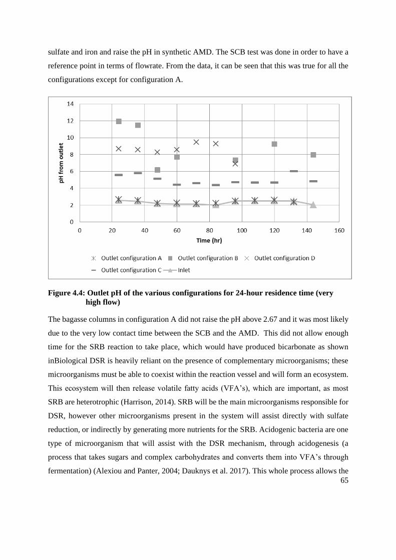
65

sulfate and iron and raise the pH in synthetic AMD. The SCB test was done in order to have a

reference point in terms of flowrate. From the data, it can be seen that this was true for all the

configurations except for configuration A.

Figure 4.4: Outlet pH of the various configurations for 24-hour residence time (very

high flow)

The bagasse columns in configuration A did not raise the pH above 2.67 and it was most likely

due to the very low contact time between the SCB and the AMD. This did not allow enough

time for the SRB reaction to take place, which would have produced bicarbonate as shown

inBiological DSR is heavily reliant on the presence of complementary microorganisms; these

microorganisms must be able to coexist within the reaction vessel and will form an ecosystem.

This ecosystem will then release volatile fatty acids (VFA’s), which are important, as most

SRB are heterotrophic (Harrison, 2014). SRB will be the main microorganisms responsible for

DSR, however other microorganisms present in the system will assist directly with sulfate

reduction, or indirectly by generating more nutrients for the SRB. Acidogenic bacteria are one

type of microorganism that will assist with the DSR mechanism, through acidogenesis (a

process that takes sugars and complex carbohydrates and converts them into VFA’s through

fermentation) (Alexiou and Panter, 2004; Dauknys et al. 2017). This whole process allows the

66

SRB to reduce sulfate to sulfide along with bicarbonate, which will raise pH, as shown in

Equation 2.6. It can also be seen from the 24 h residence time data (Figure 4.4) that the BOF

slag (all configurations except A) was able to rapidly raise the pH. These results agree with

similar work done by Name and Sheridan (2014). It is expected that the contact time between

the AMD and the BOF slag influences the level of pH rise in the system and it can be seen that

for all configurations containing BOF slag at the low contact time (high flow rate), the pH

increased to values above 10. This is above the recommended crop irrigation limits (6.5-8.2)

and indicates that in terms of alkalinity lower levels would be recommended (Grewar, 2019;

DWAF, 1996).

4.3 Acid mine drainage Treatment in process Configuration A

(bagasse and bagasse columns)

The results of the AMD treatment studies in process configuration A are presented in this

section. Configuration A is shown in Figure 4.5 for reference. In this process configuration, the

AMD was most likely treated by the biological action of the sulfate reducing bacteria in the

bagasse columns, however it is also possible that the treatment of synthetic AMD could have

occurred via the interaction between the SCB and synthetic AMD. In a biological process

sulfate is reduced to sulfide through the DSR mechanism and it is expected that the sulfide

would have formed an iron sulfide (FeS) precipitate. Iron precipitation would result in a colour

change, which was seen by the naked eye and is shown in Figure 4.3. The mechanism of pH

increase was hypothesised to be from the production of bicarbonate according to Kaksonen and

Sahinkaya (2012) and as shown in Biological DSR is heavily reliant on the presence of

complementary microorganisms; these microorganisms must be able to coexist within the

reaction vessel and will form an ecosystem. This ecosystem will then release volatile fatty acids

(VFA’s), which are important, as most SRB are heterotrophic (Harrison, 2014). SRB will be

the main microorganisms responsible for DSR, however other microorganisms present in the

system will assist directly with sulfate reduction, or indirectly by generating more nutrients for

the SRB. Acidogenic bacteria are one type of microorganism that will assist with the DSR

mechanism, through acidogenesis (a process that takes sugars and complex carbohydrates and

converts them into VFA’s through fermentation) (Alexiou and Panter, 2004; Dauknys et al.

2017). This whole process allows the SRB to reduce sulfate to sulfide along with bicarbonate,

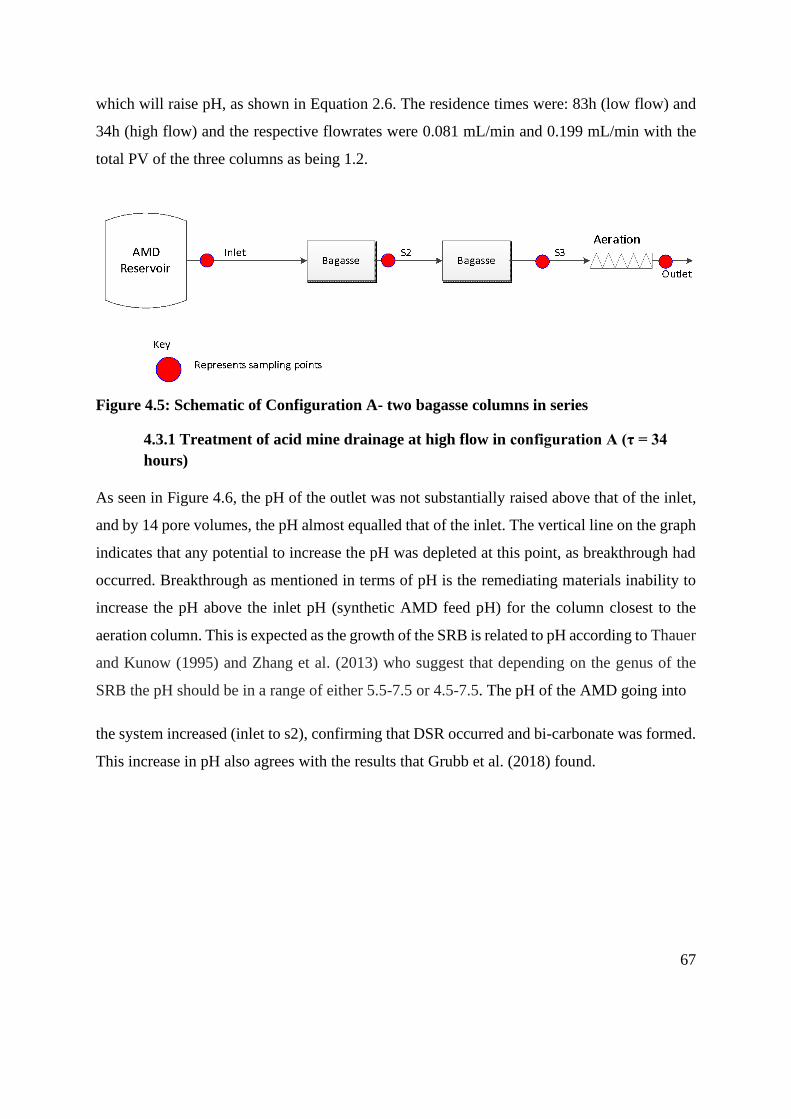
67

which will raise pH, as shown in Equation 2.6. The residence times were: 83h (low flow) and

34h (high flow) and the respective flowrates were 0.081 mL/min and 0.199 mL/min with the

total PV of the three columns as being 1.2.

Figure 4.5: Schematic of Configuration A- two bagasse columns in series

4.3.1 Treatment of acid mine drainage at high flow in configuration A (τ = 34

hours)

As seen in Figure 4.6, the pH of the outlet was not substantially raised above that of the inlet,

and by 14 pore volumes, the pH almost equalled that of the inlet. The vertical line on the graph

indicates that any potential to increase the pH was depleted at this point, as breakthrough had

occurred. Breakthrough as mentioned in terms of pH is the remediating materials inability to

increase the pH above the inlet pH (synthetic AMD feed pH) for the column closest to the

aeration column. This is expected as the growth of the SRB is related to pH according to Thauer

and Kunow (1995) and Zhang et al. (2013) who suggest that depending on the genus of the

SRB the pH should be in a range of either 5.5-7.5 or 4.5-7.5. The pH of the AMD going into

the system increased (inlet to s2), confirming that DSR occurred and bi-carbonate was formed.

This increase in pH also agrees with the results that Grubb et al. (2018) found.

68

Figure 4.6: pH as a function of pore volumes for configuration A (bagasse and bagasse

columns, 34-hour residence time)

According to a one way analysis of variance (ANOVA) results (Table 4.2), the measured pH

values were not statistically significantly different between any of the columns (s2, s3 and

outlet). This implies that the first column raised the pH to near neutral conditions and that the

second or third columns did not raise the pH beyond a statistically significantly different level.

This could indicate that column 2 was not fully acclimated and therefore did not perform as

expected. The pH increase in the first column may also have been due to the interaction

between the SCB and the synthetic AMD.

From Figure 4.7 it is seen that the sulfate concentration of the synthetic AMD decreased

consistently over the period under investigation when compared to the inlet sulfate

concentration. As mentioned previously, the SRB’s function is to reduce sulfate to sulfide and

it appears from the results that the SRB’s ability to reduce the sulfide increases with time,

however according to Thauer and Kunow (1995) the best pH for growth should have been

between a pH of 5.5 -7.5 (depending on the genus) it should be noted that Thauer and Kunow

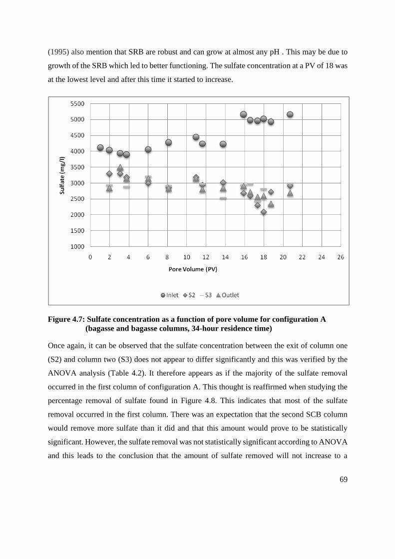
69

(1995) also mention that SRB are robust and can grow at almost any pH . This may be due to

growth of the SRB which led to better functioning. The sulfate concentration at a PV of 18 was

at the lowest level and after this time it started to increase.

Figure 4.7: Sulfate concentration as a function of pore volume for configuration A

(bagasse and bagasse columns, 34-hour residence time)

Once again, it can be observed that the sulfate concentration between the exit of column one

(S2) and column two (S3) does not appear to differ significantly and this was verified by the

ANOVA analysis (Table 4.2). It therefore appears as if the majority of the sulfate removal

occurred in the first column of configuration A. This thought is reaffirmed when studying the

percentage removal of sulfate found in Figure 4.8. This indicates that most of the sulfate

removal occurred in the first column. There was an expectation that the second SCB column

would remove more sulfate than it did and that this amount would prove to be statistically

significant. However, the sulfate removal was not statistically significant according to ANOVA

and this leads to the conclusion that the amount of sulfate removed will not increase to a

70

statistically significant level by adding more SCB columns. Another possible explanation for

this observation is that the SRB in column 2 was not functioning properly.

This sulfate and pH showed no sign of correlation and this was expected as the research did

not indicate that pH and sulfate have a major correlation, as the sulfate ion is a weak base which

supports the results shown in Figure 4.7 (Garribba et al., 2001).

Figure 4.8 also shows that initially the SRB were acclimating for the first 14 pore volumes as

the percentage sulfate removal had an increasing trend throughout their acclimation, Figure 4.8

shows that after the 16th PV the removal does not increase as drastically as the first 14. The

sulfate removal percentage increased to a maximum of 58% at PV of 18. This was the highest

removal and then it started to decrease which showed that breakthrough had started to have

occurred after a PV of 18 as the sulfate removal percentage started to decrease.

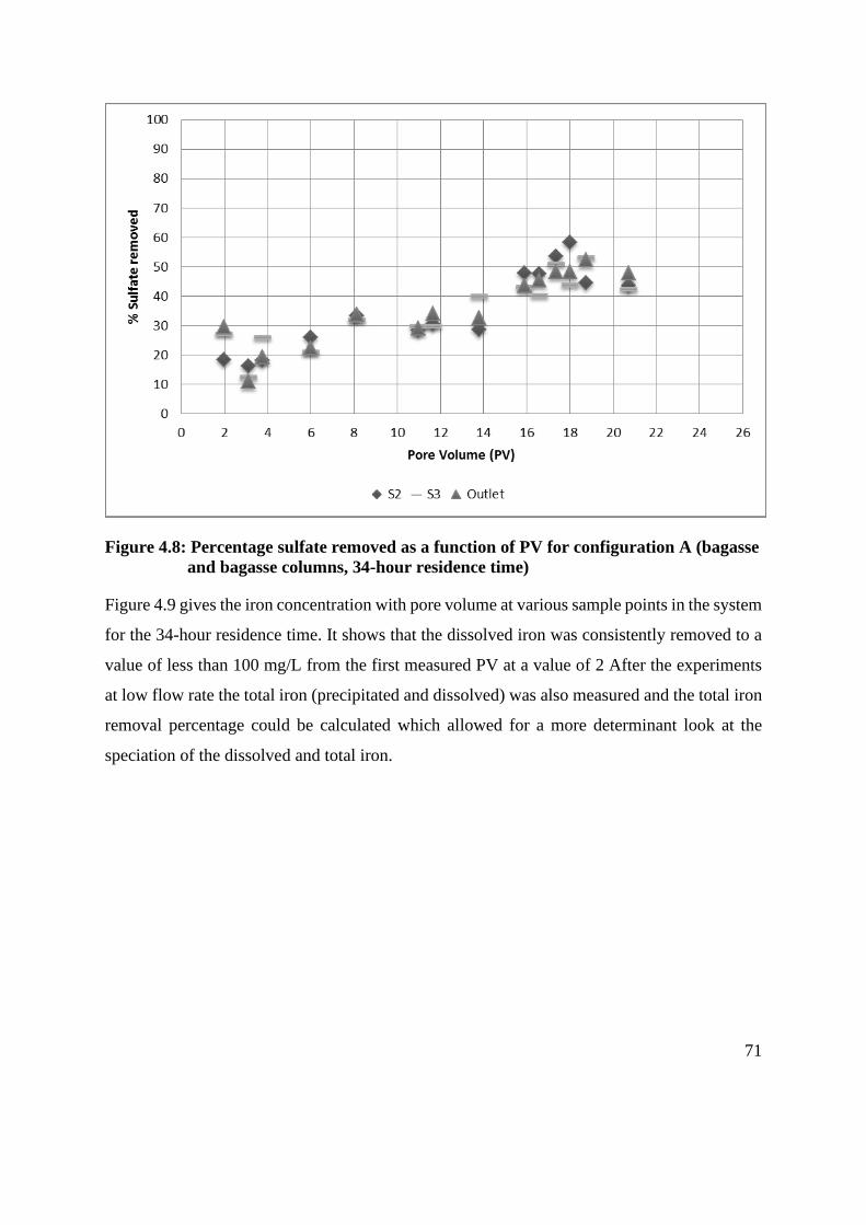
71

Figure 4.8: Percentage sulfate removed as a function of PV for configuration A (bagasse

and bagasse columns, 34-hour residence time)

Figure 4.9 gives the iron concentration with pore volume at various sample points in the system

for the 34-hour residence time. It shows that the dissolved iron was consistently removed to a

value of less than 100 mg/L from the first measured PV at a value of 2 After the experiments

at low flow rate the total iron (precipitated and dissolved) was also measured and the total iron

removal percentage could be calculated which allowed for a more determinant look at the

speciation of the dissolved and total iron.

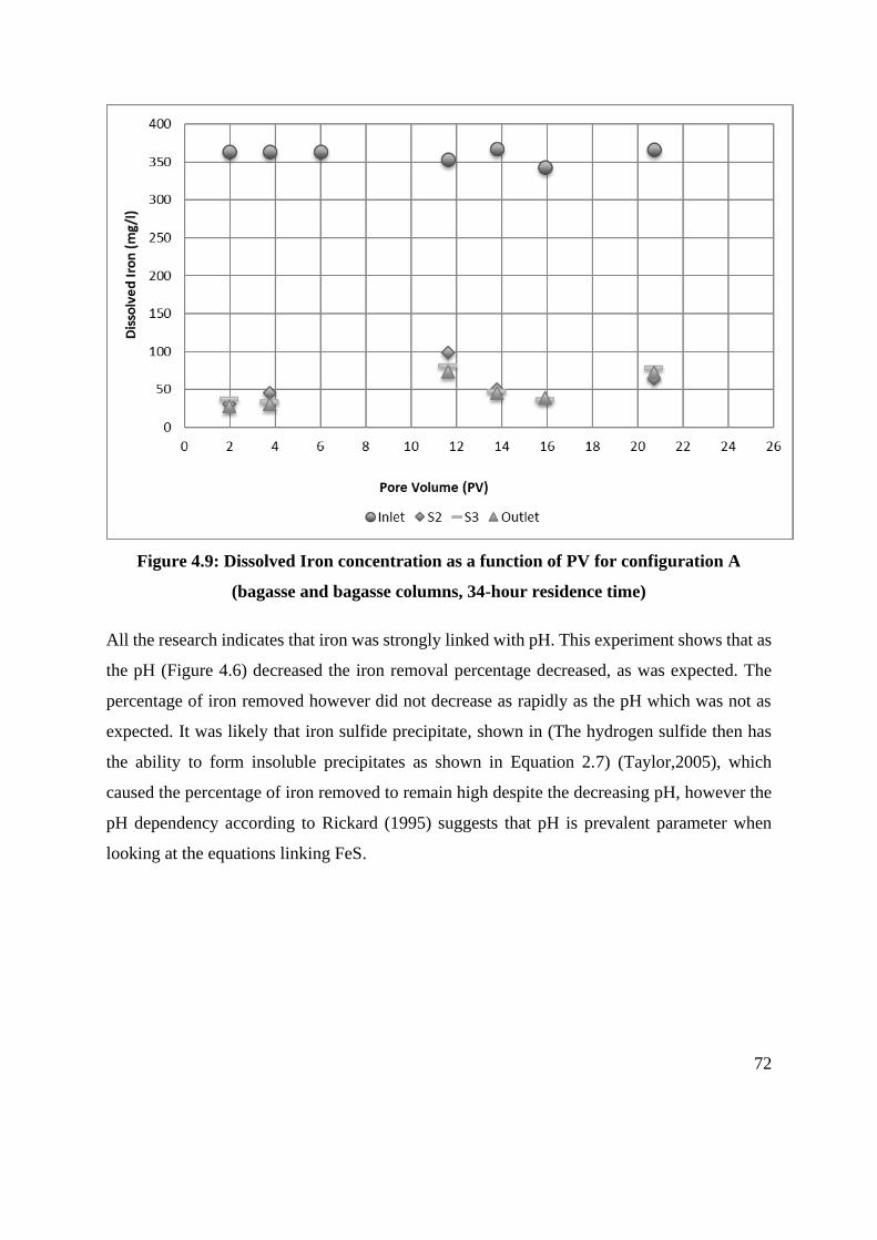
72

Figure 4.9: Dissolved Iron concentration as a function of PV for configuration A


All the research indicates that iron was strongly linked with pH. This experiment shows that as

the pH (Figure 4.6) decreased the iron removal percentage decreased, as was expected. The

percentage of iron removed however did not decrease as rapidly as the pH which was not as

expected. It was likely that iron sulfide precipitate, shown in (The hydrogen sulfide then has

the ability to form insoluble precipitates as shown in Equation 2.7) (Taylor,2005), which

caused the percentage of iron removed to remain high despite the decreasing pH, however the

pH dependency according to Rickard (1995) suggests that pH is prevalent parameter when

looking at the equations linking FeS.

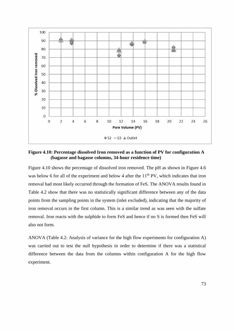
73

Figure 4.10: Percentage dissolved Iron removed as a function of PV for configuration A


Figure 4.10 shows the percentage of dissolved iron removed. The pH as shown in Figure 4.6

was below 6 for all of the experiment and below 4 after the 11th PV, which indicates that iron

removal had most likely occurred through the formation of FeS. The ANOVA results found in

Table 4.2 show that there was no statistically significant difference between any of the data

points from the sampling points in the system (inlet excluded), indicating that the majority of

iron removal occurs in the first column. This is a similar trend as was seen with the sulfate

removal. Iron reacts with the sulphide to form FeS and hence if no S is formed then FeS will

also not form.

ANOVA (Table 4.2: Analysis of variance for the high flow experiments for configuration A)

was carried out to test the null hypothesis in order to determine if there was a statistical

difference between the data from the columns within configuration A for the high flow

experiment.

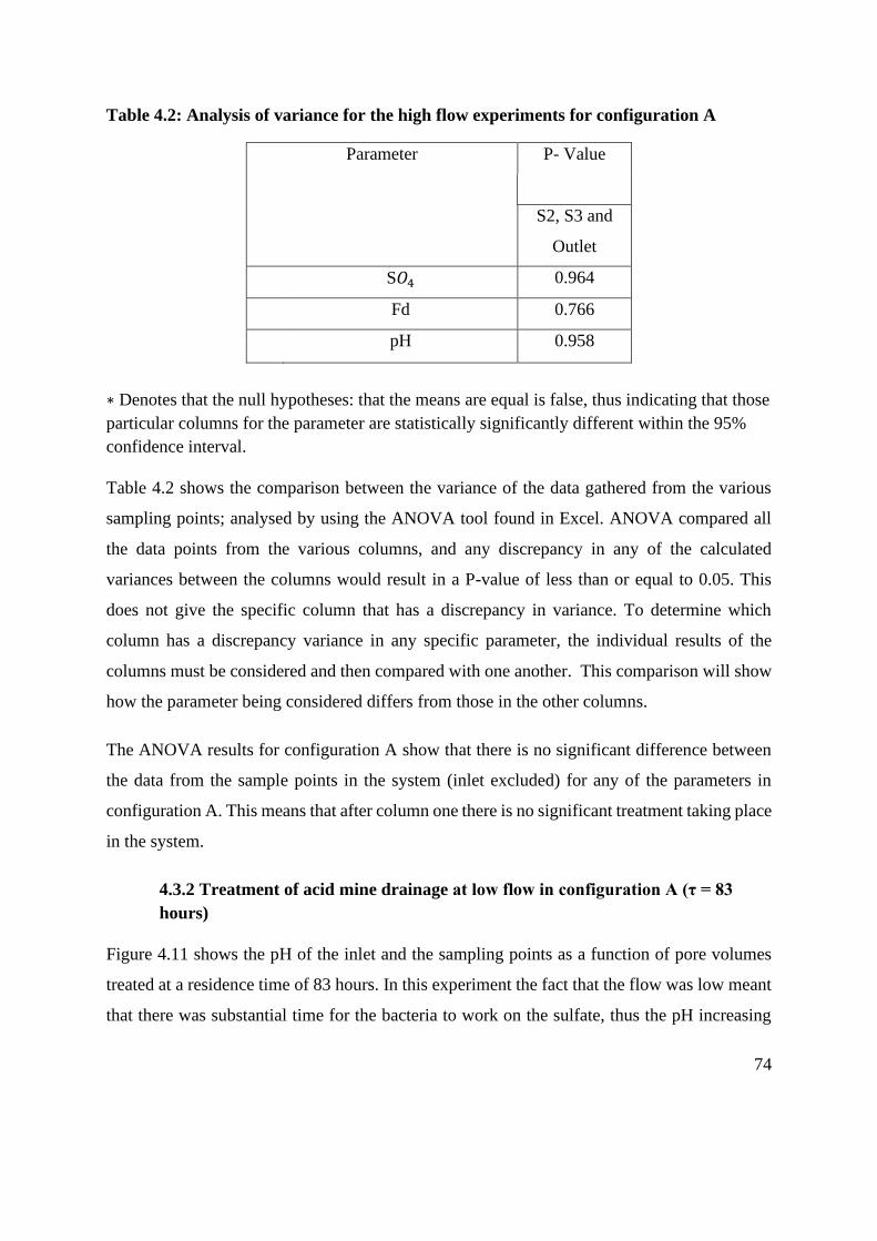
74

Table 4.2: Analysis of variance for the high flow experiments for configuration A

Parameter P- Value

S2, S3 and

Outlet

S𝑂4 0.964

Fd 0.766

pH 0.958

∗ Denotes that the null hypotheses: that the means are equal is false, thus indicating that those

particular columns for the parameter are statistically significantly different within the 95%

confidence interval.

Table 4.2 shows the comparison between the variance of the data gathered from the various

sampling points; analysed by using the ANOVA tool found in Excel. ANOVA compared all

the data points from the various columns, and any discrepancy in any of the calculated

variances between the columns would result in a P-value of less than or equal to 0.05. This

does not give the specific column that has a discrepancy in variance. To determine which

column has a discrepancy variance in any specific parameter, the individual results of the

columns must be considered and then compared with one another. This comparison will show

how the parameter being considered differs from those in the other columns.

The ANOVA results for configuration A show that there is no significant difference between

the data from the sample points in the system (inlet excluded) for any of the parameters in

configuration A. This means that after column one there is no significant treatment taking place

in the system.

4.3.2 Treatment of acid mine drainage at low flow in configuration A (τ = 83

hours)

Figure 4.11 shows the pH of the inlet and the sampling points as a function of pore volumes

treated at a residence time of 83 hours. In this experiment the fact that the flow was low meant

that there was substantial time for the bacteria to work on the sulfate, thus the pH increasing

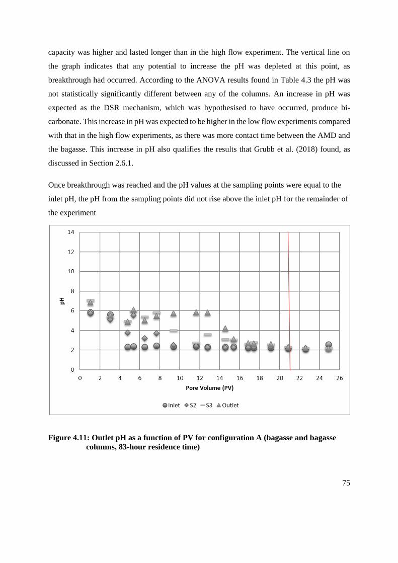
75

capacity was higher and lasted longer than in the high flow experiment. The vertical line on

the graph indicates that any potential to increase the pH was depleted at this point, as

breakthrough had occurred. According to the ANOVA results found in Table 4.3 the pH was

not statistically significantly different between any of the columns. An increase in pH was

expected as the DSR mechanism, which was hypothesised to have occurred, produce bi-

carbonate. This increase in pH was expected to be higher in the low flow experiments compared

with that in the high flow experiments, as there was more contact time between the AMD and

the bagasse. This increase in pH also qualifies the results that Grubb et al. (2018) found, as

discussed in Section 2.6.1.

Once breakthrough was reached and the pH values at the sampling points were equal to the

inlet pH, the pH from the sampling points did not rise above the inlet pH for the remainder of

the experiment

Figure 4.11: Outlet pH as a function of PV for configuration A (bagasse and bagasse


experiment.

76

Figure 4.12 shows the sulfate (SO42-) concentration of the AMD with respect to pore volume

at the inlet and at various points in process configuration A. In general, it can be seen that there

was a reduction in the concentration of sulfate from the inlet to the outlet of the process

configuration. This was an indication that the system was able to remove some of the sulfate

from solution. The sulfate concentration at a PV of 46 for the low flow experiment (Figure

4.11) was at the lowest level of sulfate concentration compared to the other sampling points

within the experiment setup.

Figure 4.12: Sulfate concentration as a function of PV for configuration A (bagasse and

bagasse columns, 83-hour residence time)

The difference between the sulfate concentration in sampling points S2, S3 and the outlet is

not significant as indicated by ANOVA found in Table 4.3, which gives an indication that the

majority of the sulfate removal occurred in the first column of configuration A. This

observation is reaffirmed by looking at the results found in Figure 4.12.

As the pH (Figure 4.11) for the low flow experiment approached near neutral conditions the

concentration of sulfate for the sampling points decreased. As the pH of the sampling points

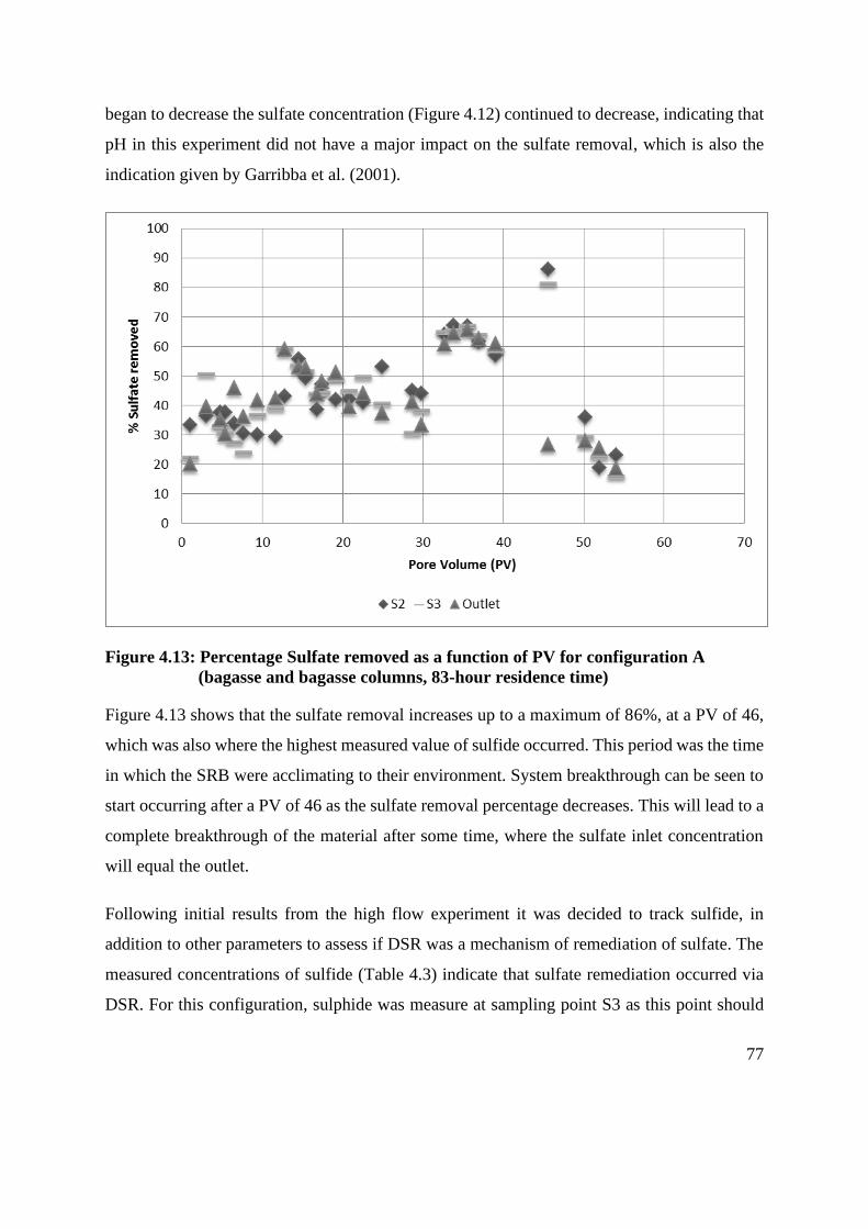
77

began to decrease the sulfate concentration (Figure 4.12) continued to decrease, indicating that

pH in this experiment did not have a major impact on the sulfate removal, which is also the

indication given by Garribba et al. (2001).

Figure 4.13: Percentage Sulfate removed as a function of PV for configuration A


Figure 4.13 shows that the sulfate removal increases up to a maximum of 86%, at a PV of 46,

which was also where the highest measured value of sulfide occurred. This period was the time

in which the SRB were acclimating to their environment. System breakthrough can be seen to

start occurring after a PV of 46 as the sulfate removal percentage decreases. This will lead to a

complete breakthrough of the material after some time, where the sulfate inlet concentration

will equal the outlet.

Following initial results from the high flow experiment it was decided to track sulfide, in

addition to other parameters to assess if DSR was a mechanism of remediation of sulfate. The

measured concentrations of sulfide (Table 4.3) indicate that sulfate remediation occurred via

DSR. For this configuration, sulphide was measure at sampling point S3 as this point should

78

have given the highest sulfide concentration as it is after both bagasse columns. Bagasse is the

carbon source for the SRB, which are responsible for the production of sulfide through the

DSR mechanism, so the sampling point closest to the column containing the bagasse should

have the highest sulfide concentration.


Measurements were taken after the point where the sulfide concentration

would be the highest. For configuration A.

Pore volume 39 44 46 50 52

Inlet

(ppm sulfide) 0.037 0.036 0.044 0.031 0.033

S3

(ppm sulfide) 0.188 0.153 0.243 0.121 0.100

Table 4.3 shows that a high sulfide concentration of 0.243 ppm was measured at a pore volume

of 46 which was when the highest sulfate removal of 86% was measured. The sulfide

concentration then decreases to a low of 0.1 ppm. This decrease in sulfide also coincides with

a decrease in sulfate percentage removal as was observed from the sulfate percentage removal

graph (Figure 4.9). This indicates that the sulfate and sulfide are linked. The sulfate and sulfide

are linked through the DSR mechanism where sulfate will be converted into sulfide (Canfield

et al., 2005).

Figure 4.14 shows that the iron concentration in the sampling points was above 200 ppm for

the majority of the measured values. Additional iron parameters are shown on this graph

compared to the low flow experiments (Figure 4.9) as further characterisation was done to

determine the speciation of dissolved (Fd) and total iron (Ft) was performed. The precipitated

iron (Fp) can be determined by subtracting dissolved iron from total iron. The removal of iron

in this experiment should have been due to the formation of iron sulfide, as the pH as shown in

Figure 4.11, had already started to go through breakthrough; this also qualifies the work done

by Grubb et al. (2018) as discussed in Section 2.6.1

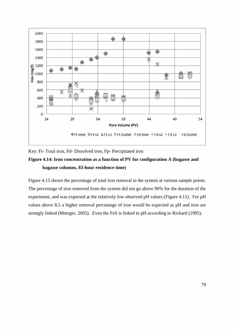
79

Key: Ft- Total iron, Fd- Dissolved iron, Fp- Precipitated iron

Figure 4.14: Iron concentration as a function of PV for configuration A (bagasse and


Figure 4.15 shows the percentage of total iron removal in the system at various sample points.

The percentage of iron removed from the system did not go above 90% for the duration of the

experiment, and was expected at the relatively low observed pH values (Figure 4.11). For pH

values above 8.5 a higher removal percentage of iron would be expected as pH and iron are

strongly linked (Metzger, 2005). Even the FeS is linked to pH according to Rickard (1995).

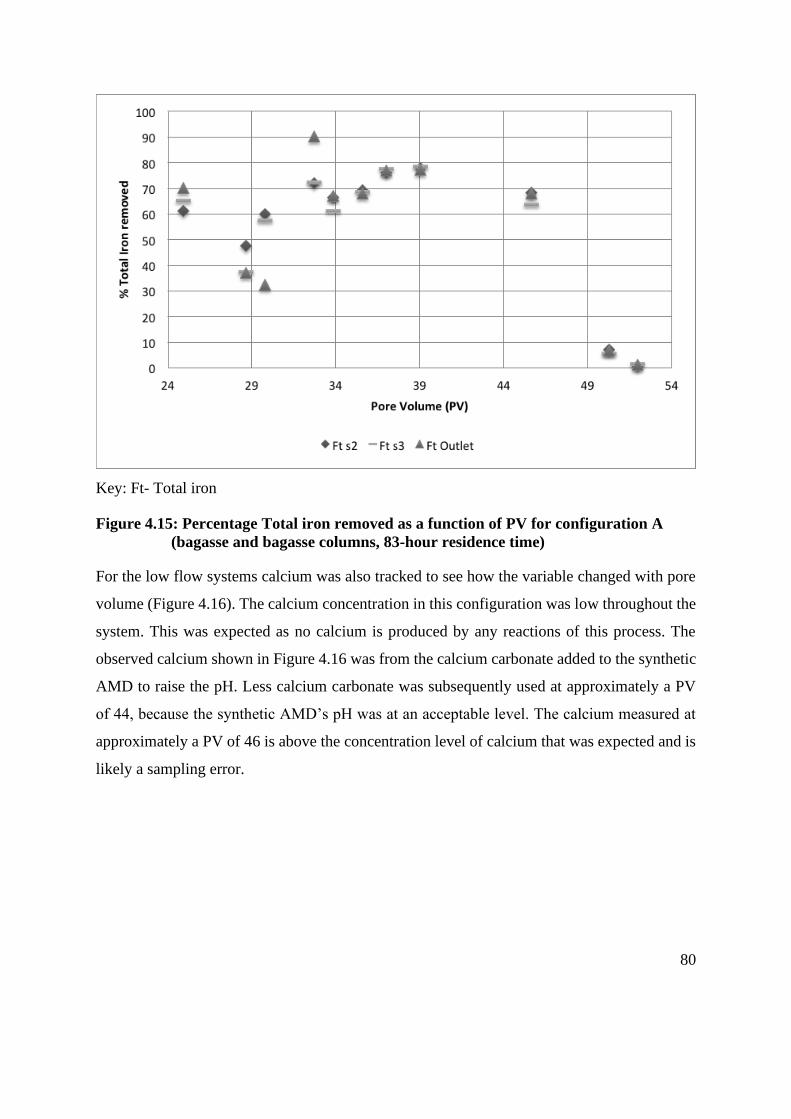
80

Key: Ft- Total iron

Figure 4.15: Percentage Total iron removed as a function of PV for configuration A


For the low flow systems calcium was also tracked to see how the variable changed with pore

volume (Figure 4.16). The calcium concentration in this configuration was low throughout the

system. This was expected as no calcium is produced by any reactions of this process. The

observed calcium shown in Figure 4.16 was from the calcium carbonate added to the synthetic

AMD to raise the pH. Less calcium carbonate was subsequently used at approximately a PV

of 44, because the synthetic AMD’s pH was at an acceptable level. The calcium measured at

approximately a PV of 46 is above the concentration level of calcium that was expected and is

likely a sampling error.

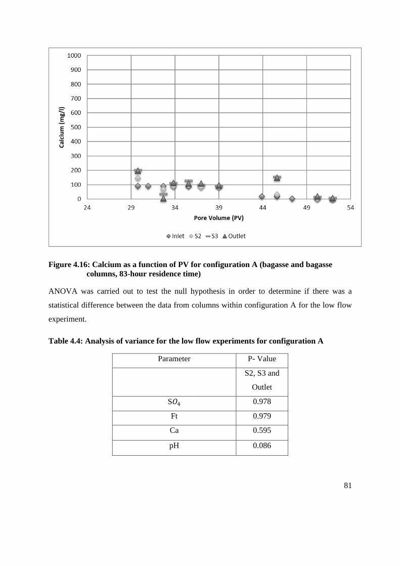
81

Figure 4.16: Calcium as a function of PV for configuration A (bagasse and bagasse


ANOVA was carried out to test the null hypothesis in order to determine if there was a

statistical difference between the data from columns within configuration A for the low flow

experiment.

Table 4.4: Analysis of variance for the low flow experiments for configuration A

Parameter P- Value

S2, S3 and

Outlet

S𝑂4 0.978

Ft 0.979

Ca 0.595

pH 0.086

82

∗ Denotes that the null hypotheses: that the means are equal was false, thus indicating that

those particular columns for the parameter are statistically significantly different within the

95% confidence interval.

The ANOVA results for configuration A show that there was no significant difference between

the measured values of any of the parameters in the columns.

4.3.3 Comparison of low and high flow treatment of AMD in process

configuration A

The pH in the very high flow experiments for configuration A (τ = 24 h) did not increase

enough for the treatment to have been considered effective, as the flow rate did not allow for

enough contact time between the AMD and the SCB (the max pH was 5.86 and the maximum

percentage removal of sulfate was 86%). If one compares the high and low flow experiments

an increase in pH is observed with a decrease in flow rate and hence increase in contact time.

The pH of the low flow experiments also stabilizes on a higher value compared to the higher

flow rates and maintains this value for a longer period. A similar trend is also seen for the other

parameters.

When the data of the high and low flow experiments are compared it can be seen that at low

flows more sulfate and iron were removed for a longer period of time, as the concentration of

both the iron and sulfate in the effluent was lower. This indicates that residence time is

important when considering sulfate and iron removal. It should be noted that as the pH of the

experiments increased or decreased the sulfate did not appear to be have been affected. The

experiments also showed that as the pH decreased the iron percentage removed decreased, as

was expected. The percentage of iron removed however did not decrease as rapidly as the pH

which was not as expected. This was likely the iron sulfide formation, which is shown in The

hydrogen sulfide then has the ability to form insoluble precipitates as shown in Equation 2.7and

is described by Taylor (2005), which caused the percentage of iron removed to remain high

despite the decreasing pH.

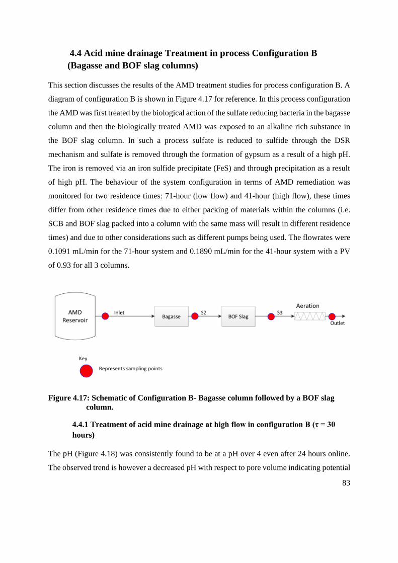
83

4.4 Acid mine drainage Treatment in process Configuration B

(Bagasse and BOF slag columns)

This section discusses the results of the AMD treatment studies for process configuration B. A

diagram of configuration B is shown in Figure 4.17 for reference. In this process configuration

the AMD was first treated by the biological action of the sulfate reducing bacteria in the bagasse

column and then the biologically treated AMD was exposed to an alkaline rich substance in

the BOF slag column. In such a process sulfate is reduced to sulfide through the DSR

mechanism and sulfate is removed through the formation of gypsum as a result of a high pH.

The iron is removed via an iron sulfide precipitate (FeS) and through precipitation as a result

of high pH. The behaviour of the system configuration in terms of AMD remediation was

monitored for two residence times: 71-hour (low flow) and 41-hour (high flow), these times

differ from other residence times due to either packing of materials within the columns (i.e.

SCB and BOF slag packed into a column with the same mass will result in different residence

times) and due to other considerations such as different pumps being used. The flowrates were

0.1091 mL/min for the 71-hour system and 0.1890 mL/min for the 41-hour system with a PV

of 0.93 for all 3 columns.

Figure 4.17: Schematic of Configuration B- Bagasse column followed by a BOF slag

column.

4.4.1 Treatment of acid mine drainage at high flow in configuration B (τ = 30

hours)

The pH (Figure 4.18) was consistently found to be at a pH over 4 even after 24 hours online.

The observed trend is however a decreased pH with respect to pore volume indicating potential

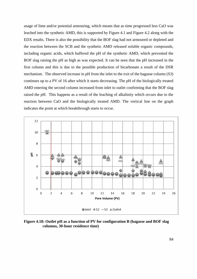
84

usage of lime and/or potential armouring, which means that as time progressed less CaO was

leached into the synthetic AMD, this is supported by Figure 4.1 and Figure 4.2 along with the

EDX results. There is also the possibility that the BOF slag had not armoured or depleted and

the reaction between the SCB and the synthetic AMD released soluble organic compounds,

including organic acids, which buffered the pH of the synthetic AMD, which prevented the

BOF slag raising the pH as high as was expected. It can be seen that the pH increased in the

first column and this is due to the possible production of bicarbonate a result of the DSR

mechanism. The observed increase in pH from the inlet to the exit of the bagasse column (S3)

continues up to a PV of 16 after which it starts decreasing. The pH of the biologically treated

AMD entering the second column increased from inlet to outlet confirming that the BOF slag

raised the pH. This happens as a result of the leaching of alkalinity which occurs due to the

reaction between CaO and the biologically treated AMD. The vertical line on the graph

indicates the point at which breakthrough starts to occur.



85

The ANOVA results indicate that there was a statistically significant difference between the

pH of the columns, considering the results from ANOVA and Figure 4.18 it can be seen that

the BOF slag was responsible for the difference in pH between the columns. Name and

Sheridan (2014) found results which confirm Figure 4.18 findings in terms of the BOF slag

and the rise in pH.

As seen in Figure 4.19, the sulfate concentration of the synthetic AMD was consistently lower

over the experiment in comparison to the inlet sulfate concentration. The first sulfate

concentration point at a PV of 1 was due to dilution effects as the percentage removal of sulfate

is higher than what would have been expected and is possibly due to dilution effects during the

measurement of the sulfate concentration. The sulfate concentration at a PV of 20 was at the

lowest level compared to the other sampling points, after this point the sulfate concentration

increases in the sample points (S2, S3 and the outlet). As mentioned previously the SRB’s

function is to reduce sulfate to sulfide and the BOF slag’s function is to raise the pH of the

synthetic AMD and precipitate sulfate as gypsum (𝐶𝑎𝑆𝑂4. 2𝐻2𝑂).

The sulfate concentration between the exit of column 1 (S2), column 2 (S3) and column 3

(outlet) does not appear to differ significantly and this is confirmed with ANOVA found in

Table 4.5. This indicates that the majority of the sulfate removal was in the first column of

configuration B. This was confirmed when studying the percentage removal of the sulfate

found in Figure 4.20. This indicates the relevance of the SCB, as the SCB is removing the

majority of the sulfate, however this could be a reflection of the position of the SCB (as the

SCB is in the first column and is then the first form of synthetic AMD treatment in this

experiment which could mean it removes the sulfate to a higher level than what the BOF slag

column can remove). This also means that having the BOF slag in the second column does not

have a significant impact on the removal of sulfate in the synthetic AMD.

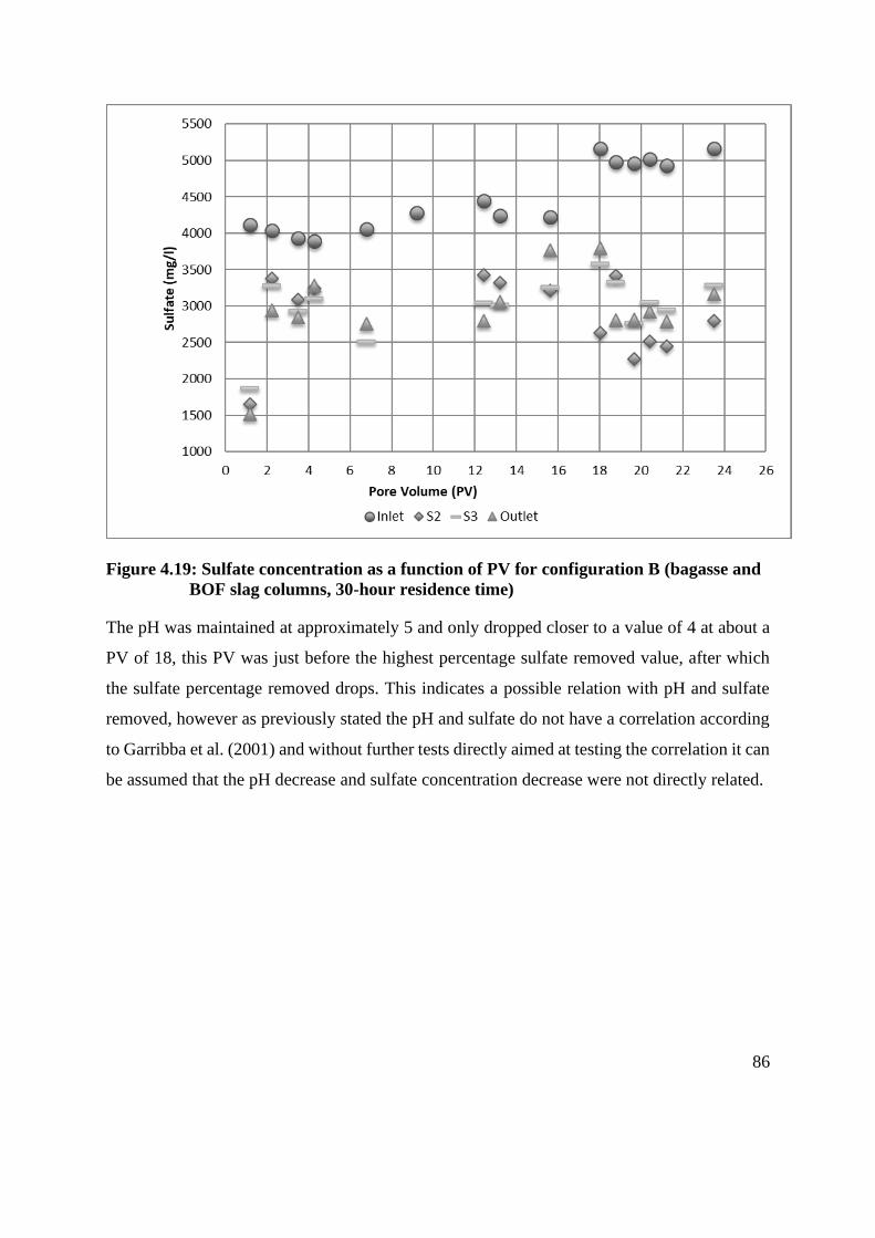
86

Figure 4.19: Sulfate concentration as a function of PV for configuration B (bagasse and

BOF slag columns, 30-hour residence time)

The pH was maintained at approximately 5 and only dropped closer to a value of 4 at about a

PV of 18, this PV was just before the highest percentage sulfate removed value, after which

the sulfate percentage removed drops. This indicates a possible relation with pH and sulfate

removed, however as previously stated the pH and sulfate do not have a correlation according

to Garribba et al. (2001) and without further tests directly aimed at testing the correlation it can

be assumed that the pH decrease and sulfate concentration decrease were not directly related.

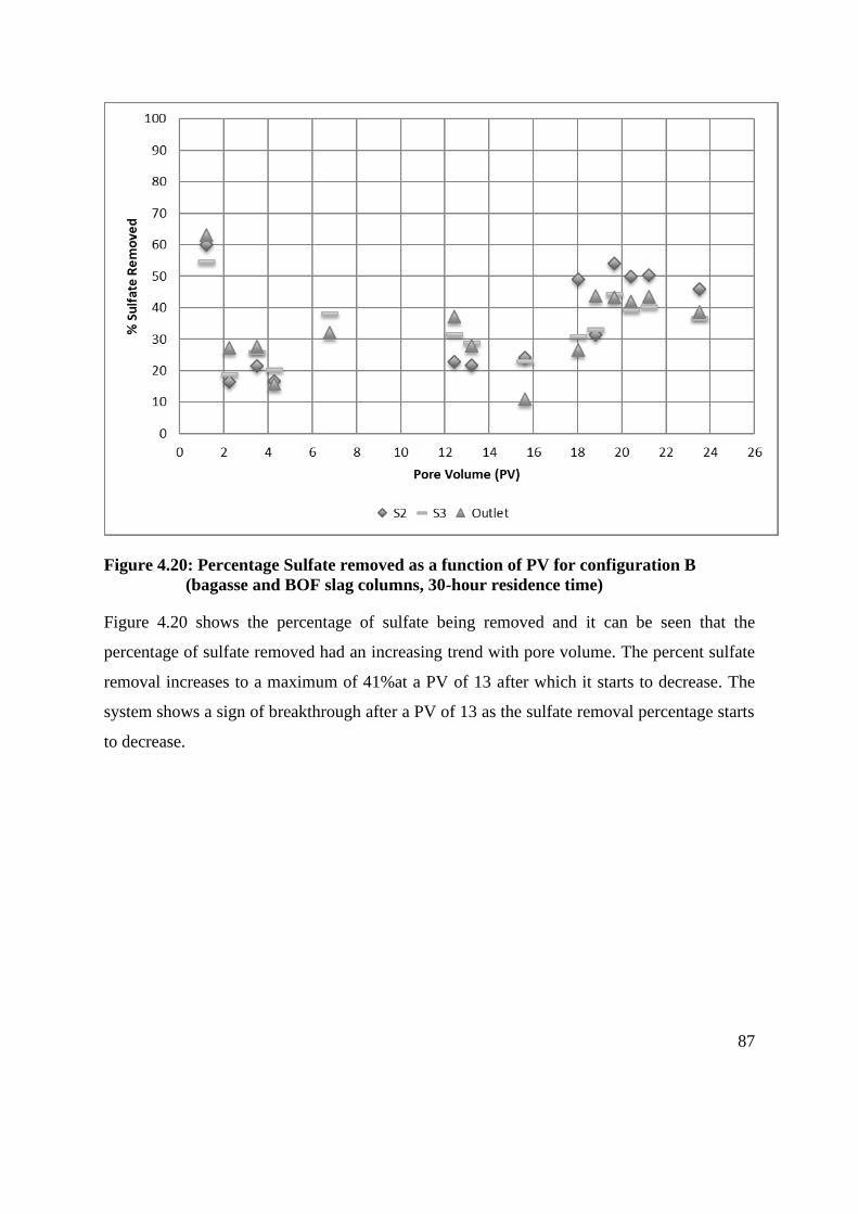
87

Figure 4.20: Percentage Sulfate removed as a function of PV for configuration B

(bagasse and BOF slag columns, 30-hour residence time)

Figure 4.20 shows the percentage of sulfate being removed and it can be seen that the

percentage of sulfate removed had an increasing trend with pore volume. The percent sulfate

removal increases to a maximum of 41%at a PV of 13 after which it starts to decrease. The

system shows a sign of breakthrough after a PV of 13 as the sulfate removal percentage starts

to decrease.

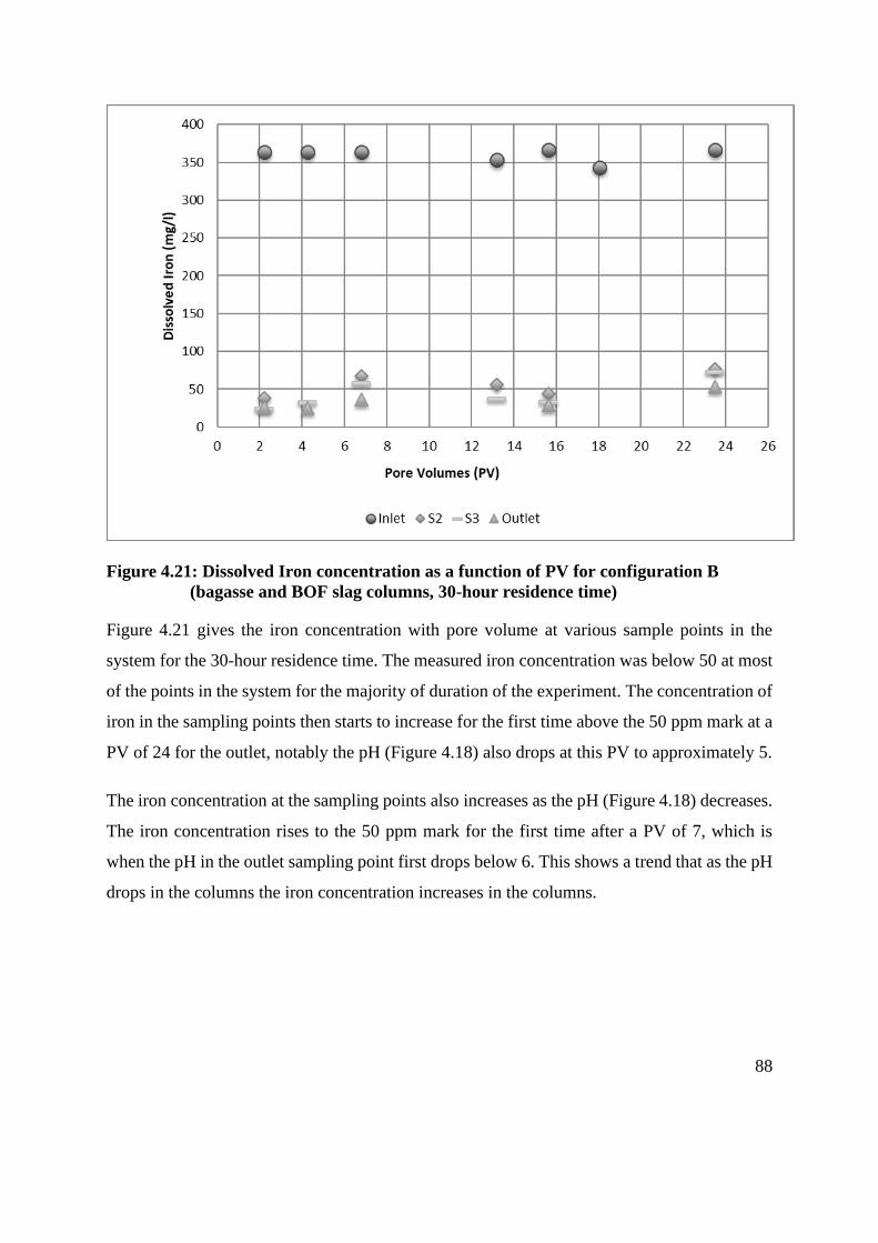
88

Figure 4.21: Dissolved Iron concentration as a function of PV for configuration B


Figure 4.21 gives the iron concentration with pore volume at various sample points in the

system for the 30-hour residence time. The measured iron concentration was below 50 at most

of the points in the system for the majority of duration of the experiment. The concentration of

iron in the sampling points then starts to increase for the first time above the 50 ppm mark at a

PV of 24 for the outlet, notably the pH (Figure 4.18) also drops at this PV to approximately 5.

The iron concentration at the sampling points also increases as the pH (Figure 4.18) decreases.

The iron concentration rises to the 50 ppm mark for the first time after a PV of 7, which is

when the pH in the outlet sampling point first drops below 6. This shows a trend that as the pH

drops in the columns the iron concentration increases in the columns.

89

Figure 4.22: Percentage Dissolved Iron removed as a function of PV for configuration B


Figure 4.22 shows the percentage of dissolved iron removed. The percentage of dissolved

iron removed reached a high of 94% at a PV of 2 and slowly decreased as the pH fell lower

until it reached a removal of 80% at a PV of 24, where the pH (Figure 4.18) had dropped to

approximately 5. ANOVA (Table 4.5) shows that there wasn’t a statistically significant

difference in iron between the columns, which was not expected, but can be explained by the

fact that the pH also did not increase very much from the inlet to the outlet of the BOF slag

column. Additionally, it was observed that the majority of iron was already removed in the

first column which was confirmed through the ANOVA analysis. Because the pH in the first

column (S2) was statistically significantly lower (ANOVA Table 4.5) than the exit pH values

of the other two columns (S3 and outlet) the majority of dissolved iron removal had most

likely happened through the formation of FeS.

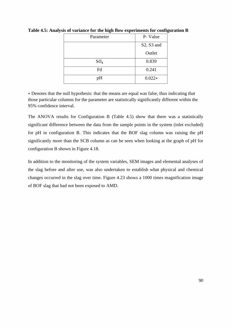
90

Table 4.5: Analysis of variance for the high flow experiments for configuration B

Parameter P- Value

S2, S3 and

Outlet

S𝑂4 0.839

Fd 0.241

pH 0.022∗

∗ Denotes that the null hypothesis: that the means are equal was false, thus indicating that



The ANOVA results for Configuration B (Table 4.5) show that there was a statistically

significant difference between the data from the sample points in the system (inlet excluded)

for pH in configuration B. This indicates that the BOF slag column was raising the pH

significantly more than the SCB column as can be seen when looking at the graph of pH for

configuration B shown in Figure 4.18.

In addition to the monitoring of the system variables, SEM images and elemental analyses of

the slag before and after use, was also undertaken to establish what physical and chemical

changes occurred in the slag over time. Figure 4.23 shows a 1000 times magnification image

of BOF slag that had not been exposed to AMD.

91

Figure 4.23: SEM results for fresh (unused) BOF slag, 1000 X magnification

The surface of the slag appears to be relatively smooth compared to the surface of the BOF

slag exposed to as shown in Figure 4.24.

Figure 4.24: SEM results for configuration B, used BOF slag, 1000 X magnification

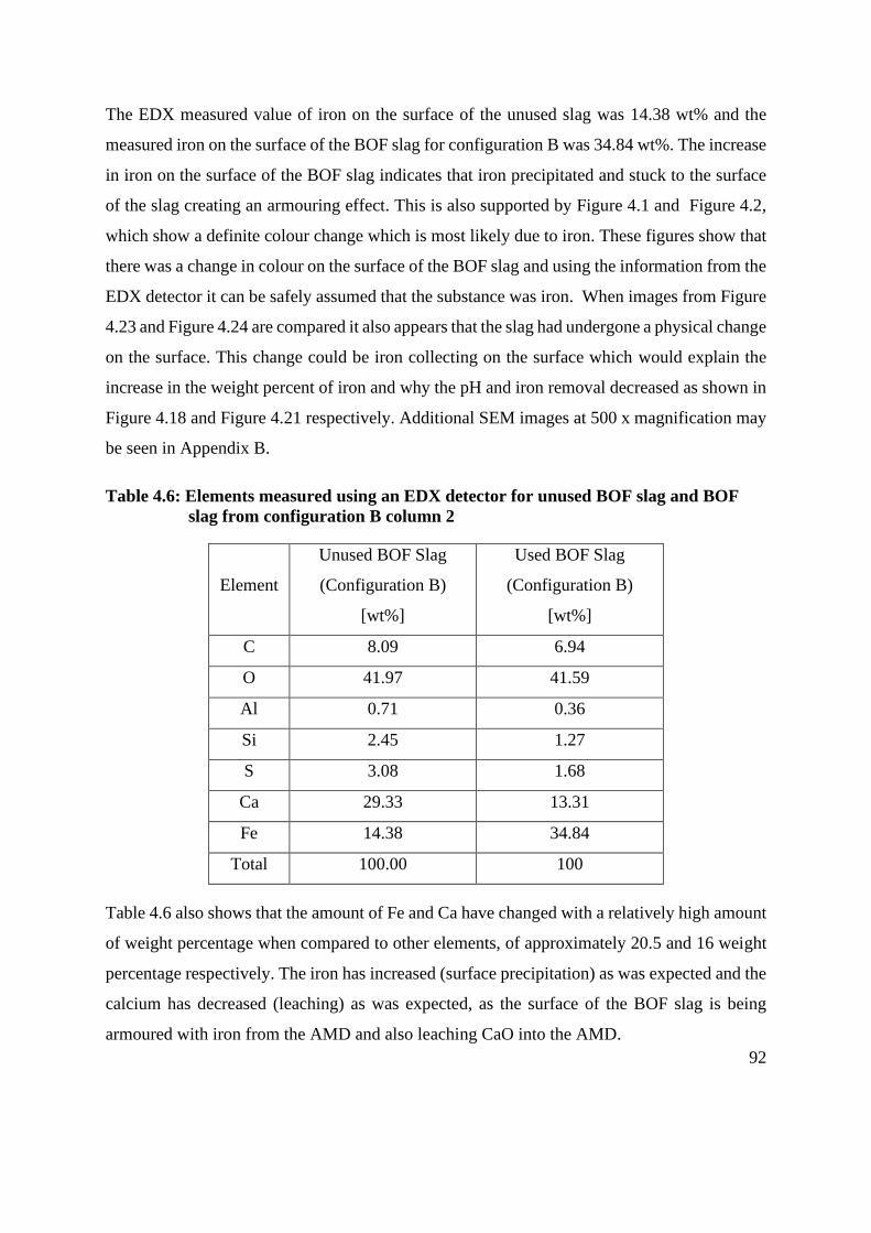
92

The EDX measured value of iron on the surface of the unused slag was 14.38 wt% and the

measured iron on the surface of the BOF slag for configuration B was 34.84 wt%. The increase

in iron on the surface of the BOF slag indicates that iron precipitated and stuck to the surface

of the slag creating an armouring effect. This is also supported by Figure 4.1 and Figure 4.2,

which show a definite colour change which is most likely due to iron. These figures show that

there was a change in colour on the surface of the BOF slag and using the information from the

EDX detector it can be safely assumed that the substance was iron. When images from Figure

4.23 and Figure 4.24 are compared it also appears that the slag had undergone a physical change

on the surface. This change could be iron collecting on the surface which would explain the

increase in the weight percent of iron and why the pH and iron removal decreased as shown in

Figure 4.18 and Figure 4.21 respectively. Additional SEM images at 500 x magnification may

be seen in Appendix B.

Table 4.6: Elements measured using an EDX detector for unused BOF slag and BOF

slag from configuration B column 2

Element

Unused BOF Slag

(Configuration B)

[wt%]

Used BOF Slag

(Configuration B)

[wt%]

C 8.09 6.94

O 41.97 41.59

Al 0.71 0.36

Si 2.45 1.27

S 3.08 1.68

Ca 29.33 13.31

Fe 14.38 34.84

Total 100.00 100

Table 4.6 also shows that the amount of Fe and Ca have changed with a relatively high amount

of weight percentage when compared to other elements, of approximately 20.5 and 16 weight

percentage respectively. The iron has increased (surface precipitation) as was expected and the

calcium has decreased (leaching) as was expected, as the surface of the BOF slag is being

armoured with iron from the AMD and also leaching CaO into the AMD.

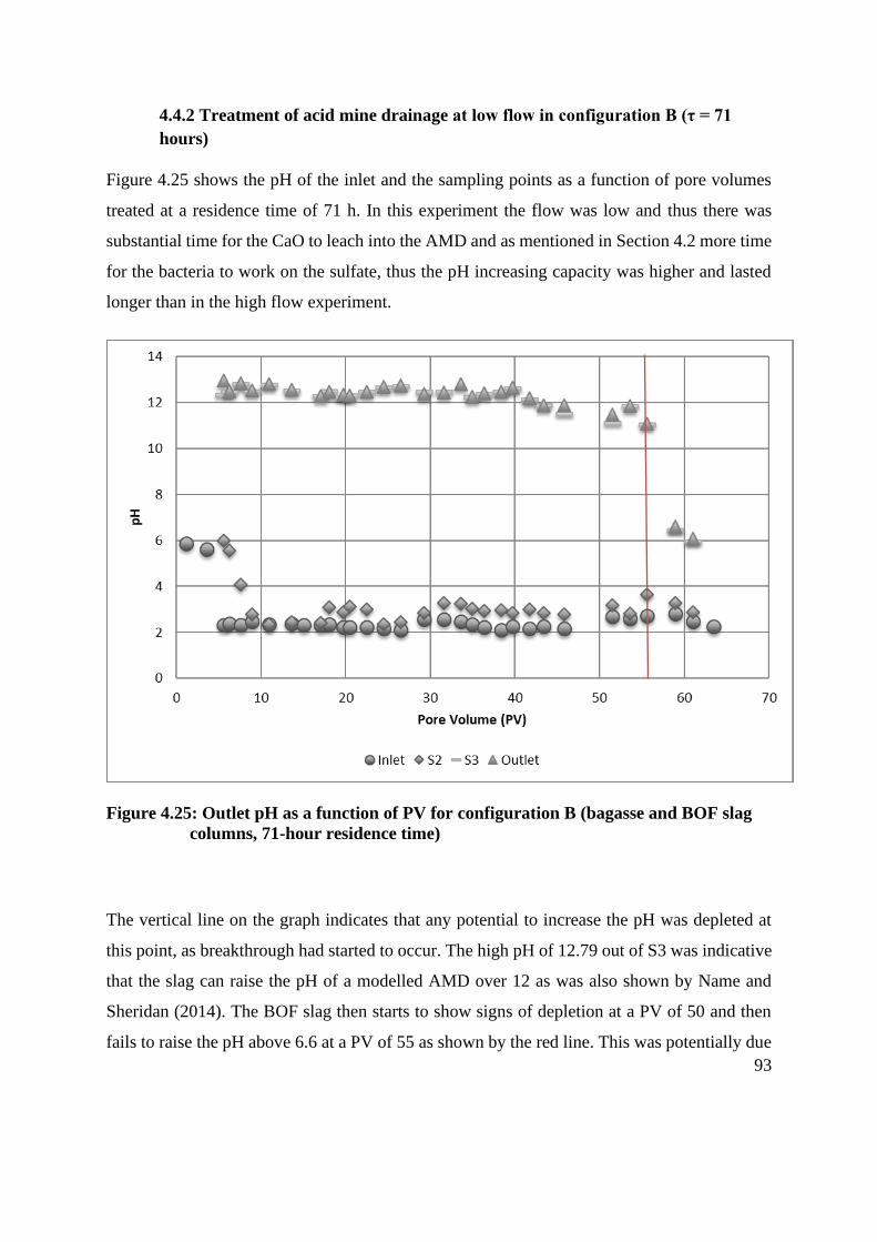
93

4.4.2 Treatment of acid mine drainage at low flow in configuration B (τ = 71

hours)

Figure 4.25 shows the pH of the inlet and the sampling points as a function of pore volumes

treated at a residence time of 71 h. In this experiment the flow was low and thus there was

substantial time for the CaO to leach into the AMD and as mentioned in Section 4.2 more time

for the bacteria to work on the sulfate, thus the pH increasing capacity was higher and lasted

longer than in the high flow experiment.



The vertical line on the graph indicates that any potential to increase the pH was depleted at

this point, as breakthrough had started to occur. The high pH of 12.79 out of S3 was indicative

that the slag can raise the pH of a modelled AMD over 12 as was also shown by Name and

Sheridan (2014). The BOF slag then starts to show signs of depletion at a PV of 50 and then

fails to raise the pH above 6.6 at a PV of 55 as shown by the red line. This was potentially due

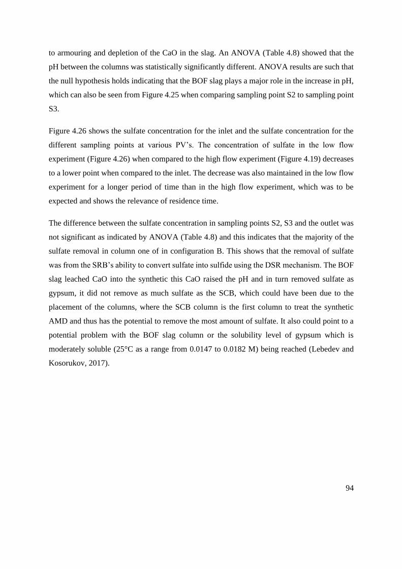
94

to armouring and depletion of the CaO in the slag. An ANOVA (Table 4.8) showed that the

pH between the columns was statistically significantly different. ANOVA results are such that

the null hypothesis holds indicating that the BOF slag plays a major role in the increase in pH,

which can also be seen from Figure 4.25 when comparing sampling point S2 to sampling point

S3.

Figure 4.26 shows the sulfate concentration for the inlet and the sulfate concentration for the

different sampling points at various PV’s. The concentration of sulfate in the low flow

experiment (Figure 4.26) when compared to the high flow experiment (Figure 4.19) decreases

to a lower point when compared to the inlet. The decrease was also maintained in the low flow

experiment for a longer period of time than in the high flow experiment, which was to be

expected and shows the relevance of residence time.

The difference between the sulfate concentration in sampling points S2, S3 and the outlet was

not significant as indicated by ANOVA (Table 4.8) and this indicates that the majority of the

sulfate removal in column one of in configuration B. This shows that the removal of sulfate

was from the SRB’s ability to convert sulfate into sulfide using the DSR mechanism. The BOF

slag leached CaO into the synthetic this CaO raised the pH and in turn removed sulfate as

gypsum, it did not remove as much sulfate as the SCB, which could have been due to the

placement of the columns, where the SCB column is the first column to treat the synthetic

AMD and thus has the potential to remove the most amount of sulfate. It also could point to a

potential problem with the BOF slag column or the solubility level of gypsum which is

moderately soluble (25°C as a range from 0.0147 to 0.0182 M) being reached (Lebedev and

Kosorukov, 2017).

95

Figure 4.26: Sulfate concentration as a function of PV for configuration B (bagasse and


Figure 4.27 shows the sulfate concentration of the AMD with respect to PV at the inlet and at

various points in process configuration B. Figure 4.27 shows that the sulfate removal increases

up to a maximum of 67%, at a PV of 40 and this was close to where the highest measured value

of sulfide was measured.

The sulfide was tracked following the initial results, because the sulfide showed that the DSR

mechanism had been a factor in the removal of sulfate. The concentration of sulfide measured

indicated that sulfate remediation had happened via DSR. The first column (bagasse) exit (s2)

was chosen for the measurement of sulfide, as the concentration of sulfide would be strongest

after the bagasse column.

96

Figure 4.27: Percentage Sulfate removed as a function of PV for configuration B




would be the highest. For configuration B.

Pore volume 46 52 54 56 59 61

Inlet

(ppm sulfide) 0.037 0.036 0.044 0.040 0.031 0.033

S2

(ppm sulfide) 0.379 0.311 0.316 0.239 0.178 0.133

The sulfate percentage removed (Figure 4.27) at a PV of 46 was high compared to the PV’s of

52, 54, 56, 59 and 61, these PV’s are relevant because it was where the sulfide concentrations

(Table 4.7) were measured. The PV of 46 occurred at the same time that the sulfide was

showing its highest percentage removed of sulfate (Figure 4.20) after this point both the sulfide

concentration and sulfate percentage removed (Figure 4.27) decreased; this indicates that the

sulfate and sulfide are linked. This link is through the DSR mechanism, where the SRB will

essentially convert sulfate into sulfide, using a carbon source such as SCB.

97

Following results shown in the Figure 4.21, a further characterisation to determine the

speciation of dissolved iron (Fd) and total iron (Ft) was performed. These results are shown in

Figure 4.28, where the total iron and dissolved iron are shown with respect to PV at the inlet

and at various sampling points.


Figure 4.28: Iron concentration as a function of PV for configuration (B bagasse and


The Ft was consistently removed throughout the experiment. The lowest concentration of total

iron occurred at the 44th PV, after which pH (Figure 4.25) breakthrough started to occur. The

pH starts to drop at a PV of 43, going under a pH of 12 for the first time in this configuration

during this experiment; the pH continues to drop until it reaches a pH of approximately 6 at a

PV of 61, which is also the PV at which the measured iron concentration was at its lowest.

During the period in which Ft and Fd were measured the iron concentration (Figure 4.29) in

the sampling point’s increases as the pH (Figure 4.25) decreases, this shows a link between the

pH and the iron. ANOVA found in Table 4.8, shows that there was a statistically significant

98

difference between the pH and also between the Ft in all columns. This difference in iron

between the columns would appear to be directly linked to the pH difference within the various

columns, which is reaffirmed when considering Figure 4.28, Figure 4.29 and Figure 4.25.

Key: Ft- Total iron

Figure 4.29: Percentage Total Iron removed as a function of PV for configuration B


Figure 4.29 shows the percentage of total iron removed at various sampling points. The highest

amount of total iron removed was 99.9% at a PV of 32 and this removal was consistently at

this level, for the S3 and outlet sample points, until a PV of 59 where it started to drop. The pH

drops under 12 (Figure 4.25) at a PV of 43, however it does not go under a pH of 10 (Figure

4.25) until the 59th PV, which was where you can see a drop in percentage of Ft to below 90%

(S3 and Outlet); potentially the slag was armouring or was depleted. The total iron removal

percentage coming out of the system at the outlet column reached a low of 72% at 61 PV’s

before the system was stopped.

The iron removal in the first column (S2) was consistently lower than the 2nd column (S3) and

outlet column, which was expected, as it was thought that the BOF slag would remove iron to

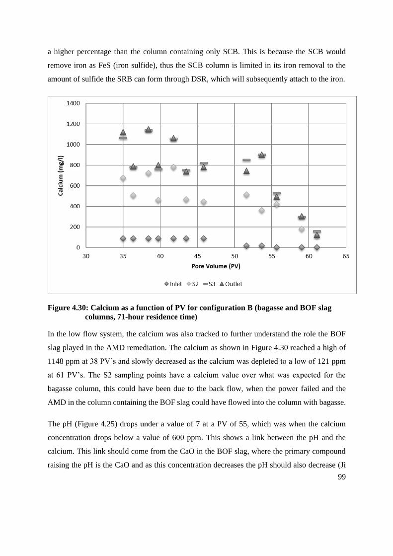
99

a higher percentage than the column containing only SCB. This is because the SCB would

remove iron as FeS (iron sulfide), thus the SCB column is limited in its iron removal to the

amount of sulfide the SRB can form through DSR, which will subsequently attach to the iron.

Figure 4.30: Calcium as a function of PV for configuration B (bagasse and BOF slag


In the low flow system, the calcium was also tracked to further understand the role the BOF

slag played in the AMD remediation. The calcium as shown in Figure 4.30 reached a high of

1148 ppm at 38 PV’s and slowly decreased as the calcium was depleted to a low of 121 ppm

at 61 PV’s. The S2 sampling points have a calcium value over what was expected for the

bagasse column, this could have been due to the back flow, when the power failed and the

AMD in the column containing the BOF slag could have flowed into the column with bagasse.

The pH (Figure 4.25) drops under a value of 7 at a PV of 55, which was when the calcium

concentration drops below a value of 600 ppm. This shows a link between the pH and the

calcium. This link should come from the CaO in the BOF slag, where the primary compound

raising the pH is the CaO and as this concentration decreases the pH should also decrease (Ji

100

et al., 2018). ANOVA results show a statistically significant difference between the calcium

between the columns, which is expected as the column containing SCB (S2) should not be

producing any calcium and the BOF slag column (S3) should have the higher calcium

concentration.

ANOVA (Table 4.8) was carried out to determine if there was a variance in the means between

the columns within configuration B for the low flow experiment. The ANOVA results for

configuration B show that there was a statistically significant difference for pH, total iron and

calcium between the columns in configuration B.

Table 4.8: Analysis of variance for the low flow experiments for configuration B

Parameter P- Value

S2, S3 and

Outlet

S𝑂4 0.983

Ft 7.299x10-

06∗

Ca 0.022∗

pH 0∗




Table 4.8 shows that there was a statistically significant difference between the columns for

the mentioned parameters; the ANOVA results together with Figure 4.25, Figure 4.29 and

Figure 4.30 indicates that the BOF slag raises the pH and removes iron to a higher percentage

than the column with only SCB. The calcium was also higher in the BOF slag column, which

was expected, due to the CaO leaching into the AMD.

101


configuration B

The pH of the very high flow experiments for configuration B initially increased to an expected

level as discussed by Name and Sheridan (2015) however the pH did not maintain a high

enough level for the treatment to be considered effective. This was due to the low contact time

between the BOF slag and the synthetic AMD and the low contact time between the SCB and

the synthetic AMD, which did not allow for the CaO from the BOF slag to leach into the AMD

or possibly did not allow enough time for the reaction between the CaO and the synthetic AMD.

It is also possible that armouring occurs early on in this experiment and thus no more alkalinity

can be leached. The low contact time between the synthetic AMD and the SCB could also

account for the relatively low pH, as the SRB may not have had enough time to acclimate. The

comparison between the high flow and low flow experiments show that an increase in pH is

observed as the flow rate decreases and this allows for a longer contact time between the

synthetic AMD and the BOF slag and SCB. This trend is seen through the other parameters.

Comparing the data from the high and low flow experiments it can be seen that at low flow

rates more sulfate and iron is removed for a longer period of time. This indicates as it did in

configuration A (Section 4.2) how important residence time is, as the longer the residence time

the greater the removal of iron and sulfate and the higher the pH is raised. The experiment

showed that sulfate and pH were not linked which was also purposed by Garribba et al. (2001),

the percentage of iron removed also decreased as the pH decreased, which is what was

expected.

4.5 Acid mine drainage Treatment in process Configuration C

(Bagasse and BOF Slag Mixed Columns)

The results for the AMD treatment studies for configuration C are presented in this section.

Configuration C is shown in Figure 4.31 and differs from configuration B in the sense that

the BOF slag (70% wt) and sugarcane bagasse (30% wt) is mixed within a column and that

there are two of these columns in series. Alkalinity leaching and sulfate reduction is therefore

combined in a single process unit. The remediation potential of the system configuration was

102

monitored for two residence times: 79 h (low flow) and 41 h (high flow) with flowrates of

0.1052 mL/min and 0.2028 mL/min respectively with a PV of 0.85.

Figure 4.31: Schematic of Configuration C- two bagasse and BOF slag mixed columns

in series

4.5.1 Treatment of acid mine drainage at high flow in configuration C (τ = 41

hours)

Figure 4.32 shows the pH at various sample points in configuration C as a function of PV.

Initially (0 < PV < 3) the pH of the synthetic AMD is raised to about 12 in column 1 and does

not increase further when it flows through column 2. At PV 3 it can be seen that the pH of the

water leaving column 1 is only raised marginally and stabilises at 5-5.5, but that column 2 still

increase the pH to 12. After PV 7 the pH in the exit of column 2 stabilizes around 6 indicating

a drop in the initial pH raise ability for the duration of the experimental run. The value at which

it stabilises corresponds well with the value obtained for the bagasse only columns seen in

configuration A. It therefore appears as if column 1 starts to breakthrough in terms of the

action of slag very fast, which is followed by the slag in column 2 starting to breakthrough. It

is believed that this might be due to armouring of the slag. The fact that a raise in pH of the

feed is still observed may due to bicarbonate produced in the DSR process. This can be

confirmed by looking at the amount of sulfate reduced in the process.

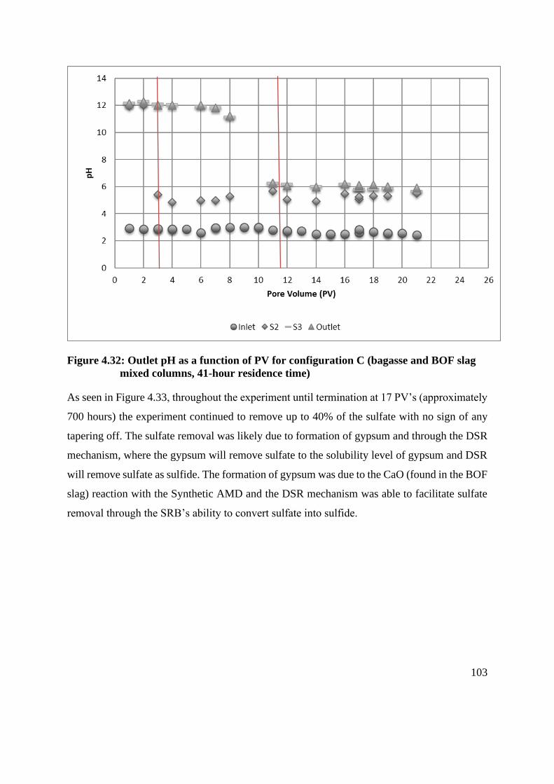
103


mixed columns, 41-hour residence time)

As seen in Figure 4.33, throughout the experiment until termination at 17 PV’s (approximately

700 hours) the experiment continued to remove up to 40% of the sulfate with no sign of any

tapering off. The sulfate removal was likely due to formation of gypsum and through the DSR

mechanism, where the gypsum will remove sulfate to the solubility level of gypsum and DSR

will remove sulfate as sulfide. The formation of gypsum was due to the CaO (found in the BOF

slag) reaction with the Synthetic AMD and the DSR mechanism was able to facilitate sulfate

removal through the SRB’s ability to convert sulfate into sulfide.

104

Figure 4.33: Sulfate concentration as a function of PV for configuration C (bagasse and

BOF slag mixed columns, 41-hour residence time)

The difference between column 1 (S2), column 2 (S3) and column 3 (outlet) does not appear

significant in terms of sulfate concentration as seen in Figure 4.33 and this was verified by

ANOVA found in Table 4.10. This indicates that the majority of the sulfate removal occurred

in the first column of configuration C. This was confirmed when studying the percentage

removal of the sulfate found in Figure 4.34.

The pH was maintained at approximately 12 in the second column for 6 PV’s and only dropped

closer to a pH of 6 at about the 11th PV. The sulfate concentration drops in relation to the feed

throughout the experiment and does not appear to be connected to the pH.

105

Figure 4.34: Percentage Sulfate removed as a function of PV for configuration C

(bagasse and BOF slag mixed columns, 41-hour residence time)

Figure 4.34 shows that the sulfate removal increases up to a maximum of 41%, at a PV of 17.

Breakthrough for this experiment was not achieved.

Figure 4.35 gives the dissolved iron concentration (Fd) with respect to PV at various sampling

points for the 41-hour residence time. The Fd was below 50 mg/L for the majority of the

experiment. The concentration of iron increases to above 50 mg/L at a PV of 17 for the first

time after column 2 (S2) and indicates that the system is losing its ability to remove iron just

after the pH (Figure 4.32) has dropped below 10.

ANOVA (Table 4.10) shows that there was no statistical significance difference between the

iron concentrations at the sampling points in the system as can be seen in Figure 4.35. This

indicates that column 1 (S2) removes the majority of the iron, which reduces the ability of

column 2 to remove iron to a higher level than column 1 as there isn’t enough iron left to

remove.

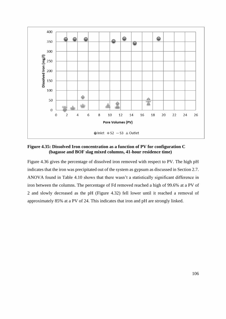
106

Figure 4.35: Dissolved Iron concentration as a function of PV for configuration C


Figure 4.36 gives the percentage of dissolved iron removed with respect to PV. The high pH

indicates that the iron was precipitated out of the system as gypsum as discussed in Section 2.7.

ANOVA found in Table 4.10 shows that there wasn’t a statistically significant difference in

iron between the columns. The percentage of Fd removed reached a high of 99.6% at a PV of

2 and slowly decreased as the pH (Figure 4.32) fell lower until it reached a removal of

approximately 85% at a PV of 24. This indicates that iron and pH are strongly linked.

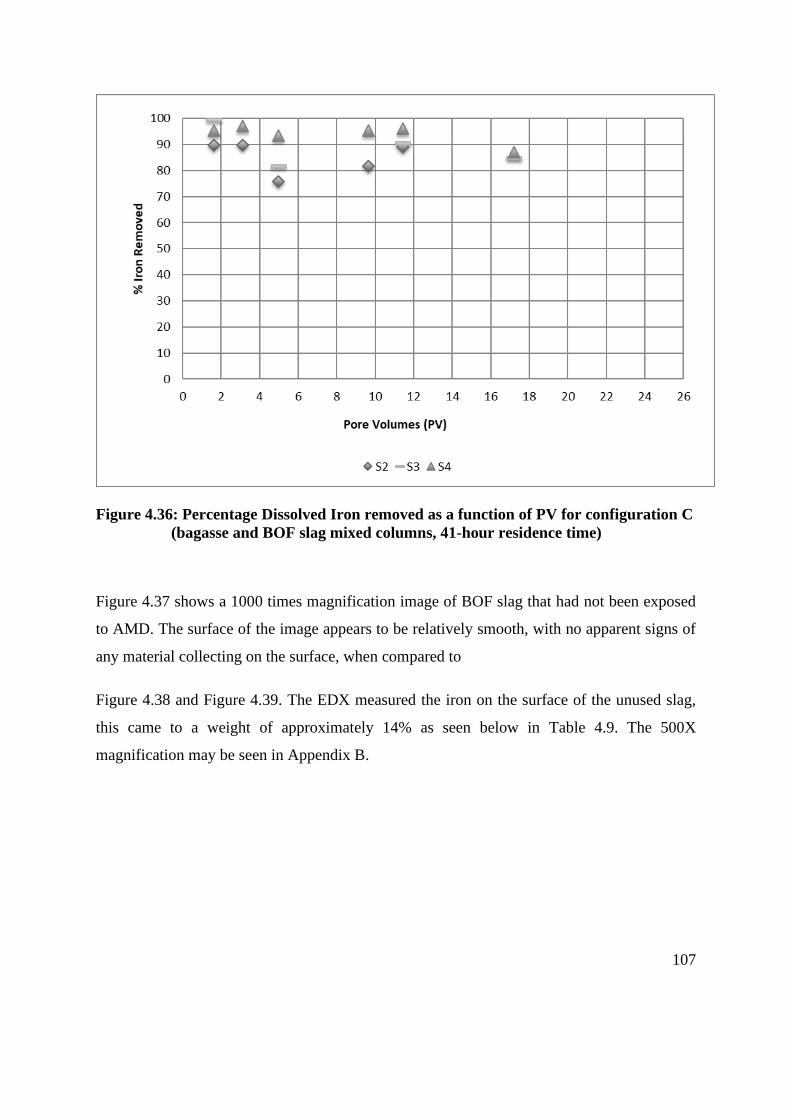
107

Figure 4.36: Percentage Dissolved Iron removed as a function of PV for configuration C


Figure 4.37 shows a 1000 times magnification image of BOF slag that had not been exposed

to AMD. The surface of the image appears to be relatively smooth, with no apparent signs of

any material collecting on the surface, when compared to

Figure 4.38 and Figure 4.39. The EDX measured the iron on the surface of the unused slag,

this came to a weight of approximately 14% as seen below in Table 4.9. The 500X

magnification may be seen in Appendix B.

108


Figure 4.38: SEM results for configuration C, used BOF slag from the first column,

1000 X magnification

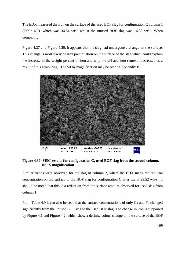
109

The EDX measured the iron on the surface of the used BOF slag for configuration C column 1

(Table 4.9), which was 34.84 wt% whilst the unused BOF slag was 14.38 wt%. When

comparing

Figure 4.37 and Figure 4.39, it appears that the slag had undergone a change on the surface.

This change is most likely be iron precipitation on the surface of the slag which could explain

the increase in the weight percent of iron and why the pH and iron removal decreased as a

result of this armouring. The 500X magnification may be seen in Appendix B.

Figure 4.39: SEM results for configuration C, used BOF slag from the second column,

1000 X magnification

Similar trends were observed for the slag in column 2, where the EDX measured the iron

concentration on the surface of the BOF slag for configuration C after use at 29.52 wt% It

should be noted that this is a reduction from the surface amount observed for used slag from

column 1.

From Table 4.9 it can also be seen that the surface concentrations of only Ca and Fe changed

significantly from the unused BOF slag to the used BOF slag. The change in iron is supported

by Figure 4.1 and Figure 4.2, which show a definite colour change on the surface of the BOF

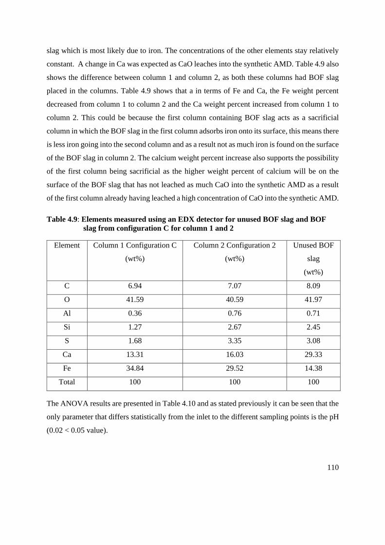
110

slag which is most likely due to iron. The concentrations of the other elements stay relatively

constant. A change in Ca was expected as CaO leaches into the synthetic AMD. Table 4.9 also

shows the difference between column 1 and column 2, as both these columns had BOF slag

placed in the columns. Table 4.9 shows that a in terms of Fe and Ca, the Fe weight percent

decreased from column 1 to column 2 and the Ca weight percent increased from column 1 to

column 2. This could be because the first column containing BOF slag acts as a sacrificial

column in which the BOF slag in the first column adsorbs iron onto its surface, this means there

is less iron going into the second column and as a result not as much iron is found on the surface

of the BOF slag in column 2. The calcium weight percent increase also supports the possibility

of the first column being sacrificial as the higher weight percent of calcium will be on the

surface of the BOF slag that has not leached as much CaO into the synthetic AMD as a result

of the first column already having leached a high concentration of CaO into the synthetic AMD.


slag from configuration C for column 1 and 2

Element Column 1 Configuration C

(wt%)

Column 2 Configuration 2

(wt%)

Unused BOF

slag

(wt%)

C 6.94 7.07 8.09

O 41.59 40.59 41.97

Al 0.36 0.76 0.71

Si 1.27 2.67 2.45

S 1.68 3.35 3.08

Ca 13.31 16.03 29.33

Fe 34.84 29.52 14.38

Total 100 100 100

The ANOVA results are presented in Table 4.10 and as stated previously it can be seen that the

only parameter that differs statistically from the inlet to the different sampling points is the pH

(0.02 < 0.05 value).

111

Table 4.10: Analysis of variance for the high flow experiments for configuration C

Parameter P- Value

S2, S3 and

Outlet

S𝑂4 0.356

Fd 0.246

pH 0.020∗




4.5.2 Treatment of acid mine drainage at low flow in configuration C (τ = 79

hours)

Figure 4.40 shows the pH at the inlet and the sampling points. In this experiment the flow

was low and thus there was substantial time for the bacteria to work on the sulfate and more

time for the lime to leach into the AMD, thus the pH increasing capacity was higher and

lasted longer than in the high flow experiment.

The vertical lines on the graph indicate that any potential to increase the pH was depleted at

this point. The first line was for the first column and the second line was for the second column.

The high pH of 12.82 out at S3 was indicative that the slag can raise the pH of a modelled

AMD to over 12 as was also shown by Name and Sheridan (2014). The BOF slag then starts

to show signs of depletion at a PV of 10 for the first column and then at a PV of 20 for the

second column. This was potentially due to armouring and depletion of the slag.

The pH between the columns was statistically significantly different as shown by Table 4.12.

ANOVA results are such that the null hypothesis, that the means are equal was false, indicating

that the BOF slag plays a major role in pH production, which can also be seen from Figure

4.40, when comparing sampling point S2 to sampling point S3.

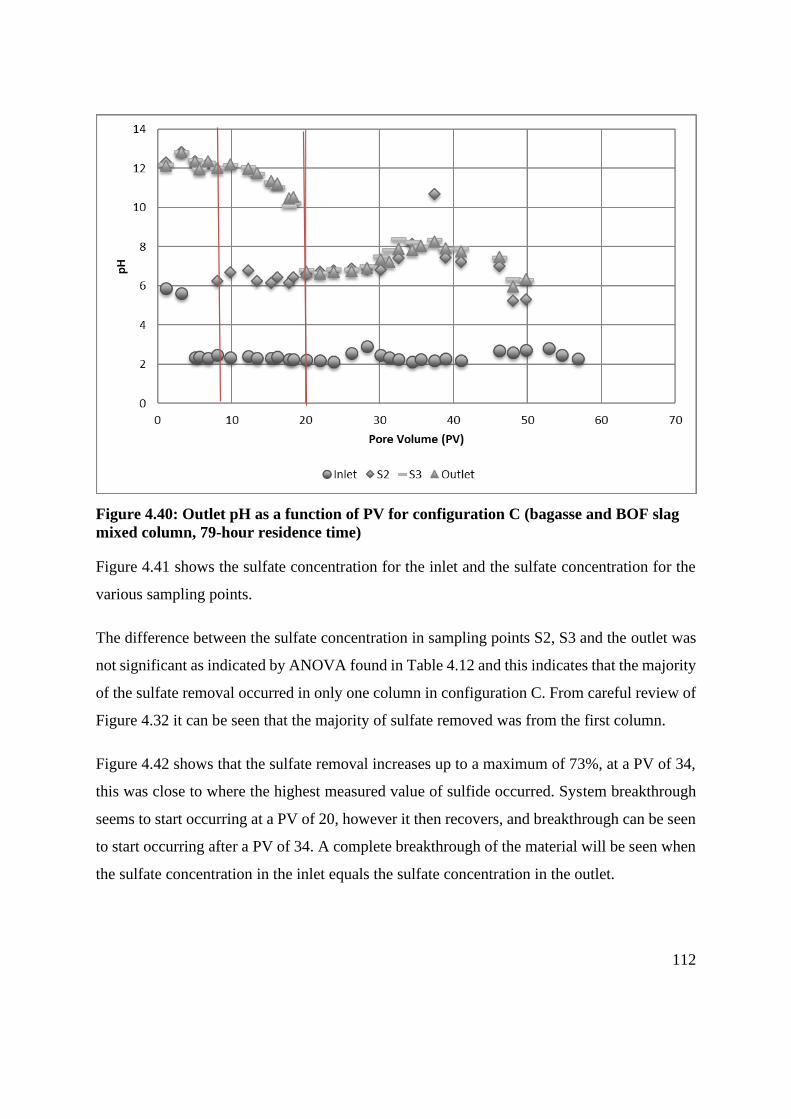
112


mixed column, 79-hour residence time)


various sampling points.


not significant as indicated by ANOVA found in Table 4.12 and this indicates that the majority

of the sulfate removal occurred in only one column in configuration C. From careful review of

Figure 4.32 it can be seen that the majority of sulfate removed was from the first column.

Figure 4.42 shows that the sulfate removal increases up to a maximum of 73%, at a PV of 34,

this was close to where the highest measured value of sulfide occurred. System breakthrough

seems to start occurring at a PV of 20, however it then recovers, and breakthrough can be seen

to start occurring after a PV of 34. A complete breakthrough of the material will be seen when

the sulfate concentration in the inlet equals the sulfate concentration in the outlet.

113

Figure 4.41: Sulfate concentration as a function of PV for configuration C (bagasse and


The measured concentration of sulfide (Table 4.11) indicates that sulfate remediation occurred

via DSR. The column closest to the outlet point containing bagasse was chosen for the

measurement of sulfide, as the concentration of sulfide would be strongest after the bagasse

column nearest to the aeration column. Sampling point S3 was done for configuration C.

The sulfate concentration shown in Figure 4.41 at a PV of 41 was low compared to the PV’s

of 46, 48, 50, 53 and 58, these PV’s are relevant because it was where the sulfide

concentrations were measured.

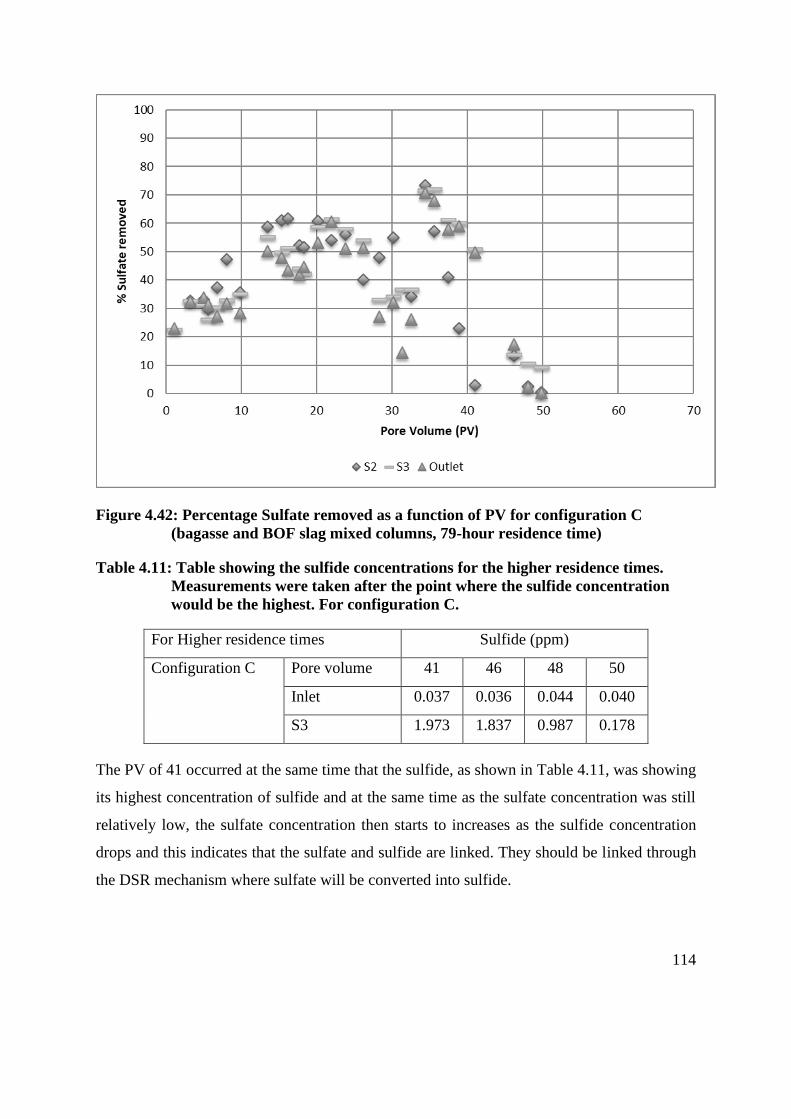
114

Figure 4.42: Percentage Sulfate removed as a function of PV for configuration C




would be the highest. For configuration C.

For Higher residence times Sulfide (ppm)

Configuration C Pore volume 41 46 48 50

Inlet 0.037 0.036 0.044 0.040

S3 1.973 1.837 0.987 0.178

The PV of 41 occurred at the same time that the sulfide, as shown in Table 4.11, was showing

its highest concentration of sulfide and at the same time as the sulfate concentration was still

relatively low, the sulfate concentration then starts to increases as the sulfide concentration

drops and this indicates that the sulfate and sulfide are linked. They should be linked through

the DSR mechanism where sulfate will be converted into sulfide.

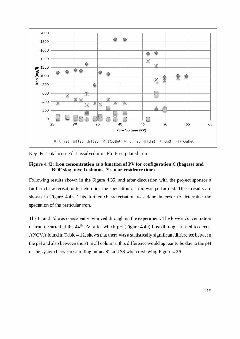
115


Figure 4.43: Iron concentration as a function of PV for configuration C (bagasse and


Following results shown in the Figure 4.35, and after discussion with the project sponsor a

further characterisation to determine the speciation of iron was performed. These results are

shown in Figure 4.43. This further characterisation was done in order to determine the

speciation of the particular iron.

The Ft and Fd was consistently removed throughout the experiment. The lowest concentration

of iron occurred at the 44th PV, after which pH (Figure 4.40) breakthrough started to occur.

ANOVA found in Table 4.12, shows that there was a statistically significant difference between

the pH and also between the Ft in all columns, this difference would appear to be due to the pH

of the system between sampling points S2 and S3 when reviewing Figure 4.35.

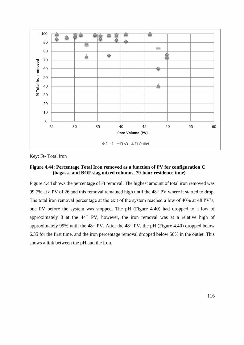
116

Key: Ft- Total iron

Figure 4.44: Percentage Total Iron removed as a function of PV for configuration C


Figure 4.44 shows the percentage of Ft removal. The highest amount of total iron removed was

99.7% at a PV of 26 and this removal remained high until the 48th PV where it started to drop.

The total iron removal percentage at the exit of the system reached a low of 40% at 48 PV’s,

one PV before the system was stopped. The pH (Figure 4.40) had dropped to a low of

approximately 8 at the 44th PV, however, the iron removal was at a relative high of

approximately 99% until the 48th PV. After the 48th PV, the pH (Figure 4.40) dropped below

6.35 for the first time, and the iron percentage removal dropped below 50% in the outlet. This

shows a link between the pH and the iron.

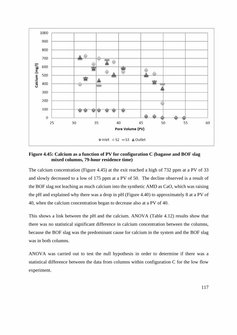
117

Figure 4.45: Calcium as a function of PV for configuration C (bagasse and BOF slag

mixed columns, 79-hour residence time)

The calcium concentration (Figure 4.45) at the exit reached a high of 732 ppm at a PV of 33

and slowly decreased to a low of 175 ppm at a PV of 50. The decline observed is a result of

the BOF slag not leaching as much calcium into the synthetic AMD as CaO, which was raising

the pH and explained why there was a drop in pH (Figure 4.40) to approximately 8 at a PV of

40, when the calcium concentration began to decrease also at a PV of 40.

This shows a link between the pH and the calcium. ANOVA (Table 4.12) results show that

there was no statistical significant difference in calcium concentration between the columns,

because the BOF slag was the predominant cause for calcium in the system and the BOF slag

was in both columns.


statistical difference between the data from columns within configuration C for the low flow

experiment.

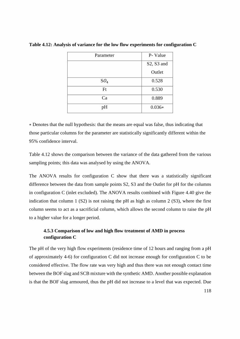
118

Table 4.12: Analysis of variance for the low flow experiments for configuration C

Parameter P- Value

S2, S3 and

Outlet

S𝑂4 0.528

Ft 0.530

Ca 0.889

pH 0.036∗




Table 4.12 shows the comparison between the variance of the data gathered from the various

sampling points; this data was analysed by using the ANOVA.

The ANOVA results for configuration C show that there was a statistically significant

difference between the data from sample points S2, S3 and the Outlet for pH for the columns

in configuration C (inlet excluded). The ANOVA results combined with Figure 4.40 give the

indication that column 1 (S2) is not raising the pH as high as column 2 (S3), where the first

column seems to act as a sacrificial column, which allows the second column to raise the pH

to a higher value for a longer period.


configuration C

The pH of the very high flow experiments (residence time of 12 hours and ranging from a pH

of approximately 4-6) for configuration C did not increase enough for configuration C to be

considered effective. The flow rate was very high and thus there was not enough contact time

between the BOF slag and SCB mixture with the synthetic AMD. Another possible explanation

is that the BOF slag armoured, thus the pH did not increase to a level that was expected. Due

119

to the limited contact time or possible armouring between the BOF slag and SCB mixture with

the synthetic AMD, the pH of the synthetic AMD, did not increase enough for the treatment to

be considered effective. Effective in this experiment meant raising the pH high enough to

remove most heavy metals (a pH of 9.5 and above) and effective in terms of reaching the levels

proposed by Name and Sheridan (2015).

When comparing the high and low flow experiments it can be seen that as the residence time

increases the percentage sulfate removal, percentage iron removal and pH all increase, which

is most likely due to the increase in contact time between the BOF slag and SCB mixture and

the synthetic AMD. The pH (Figure 4.40) and total iron percentage removal (Figure 4.44)

appear to be linked, because after the pH drops the iron drops within 4 PV’s. It can also be seen

that in the two experiments the first column containing a mixture of SCB and BOF slag started

to experience breakthrough before the second column which had the same mixture, and this

was expected and shows how the first column can act as a sacrificial column which mitigates

the armouring effect for a period of time within the second column.

4.6 Acid mine drainage Treatment in process Configuration D (BOF

slag and Bagasse Columns)

This section shows the results of the AMD treatment studies for process configuration D. A

diagram of process configuration D is shown in Figure 4.46 as a point of reference. In this

process configuration the AMD was high-pH treated with an alkaline rich substance (the BOF

slag) column 1 and it then should have been treated by the biological action of the sulfate

reducing bacteria in the bagasse column, column 2. In such a process sulfate is removed as

gypsum through precipitation, to the solubility limit of gypsum (25°C in water as a range from

0.0147 to 0.0182 M), as a result of a high pH in the first column and then the sulfate should

also be removed as a metal precipitate or hydrogen sulfide gas through the DSR process in the

second column (Lebedev and Kosorukov, 2017). The system was monitored in terms of AMD

remediation for two residence times: 86-hour (low flow) and 37-hour (high flow) with

flowrates of 0.0901 mL/min and 0.2095 mL/min with a PV of 0.96.

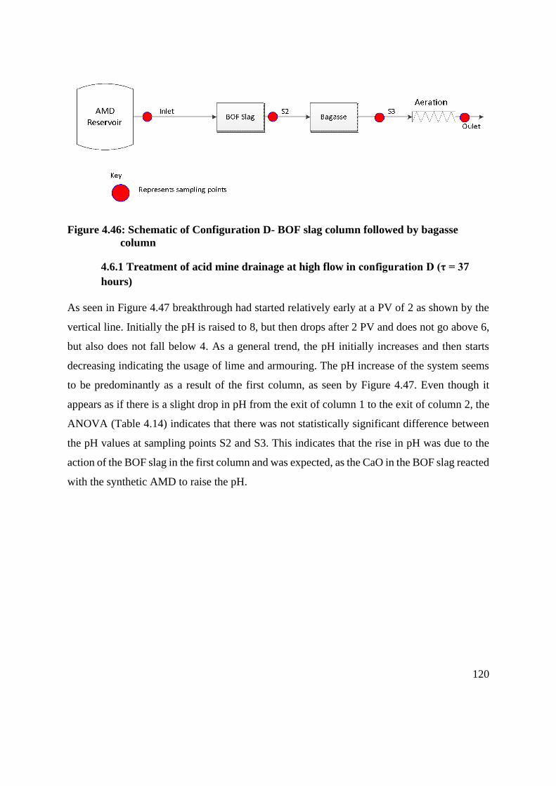
120

Figure 4.46: Schematic of Configuration D- BOF slag column followed by bagasse

column

4.6.1 Treatment of acid mine drainage at high flow in configuration D (τ = 37

hours)

As seen in Figure 4.47 breakthrough had started relatively early at a PV of 2 as shown by the

vertical line. Initially the pH is raised to 8, but then drops after 2 PV and does not go above 6,

but also does not fall below 4. As a general trend, the pH initially increases and then starts

decreasing indicating the usage of lime and armouring. The pH increase of the system seems

to be predominantly as a result of the first column, as seen by Figure 4.47. Even though it

appears as if there is a slight drop in pH from the exit of column 1 to the exit of column 2, the

ANOVA (Table 4.14) indicates that there was not statistically significant difference between

the pH values at sampling points S2 and S3. This indicates that the rise in pH was due to the

action of the BOF slag in the first column and was expected, as the CaO in the BOF slag reacted

with the synthetic AMD to raise the pH.

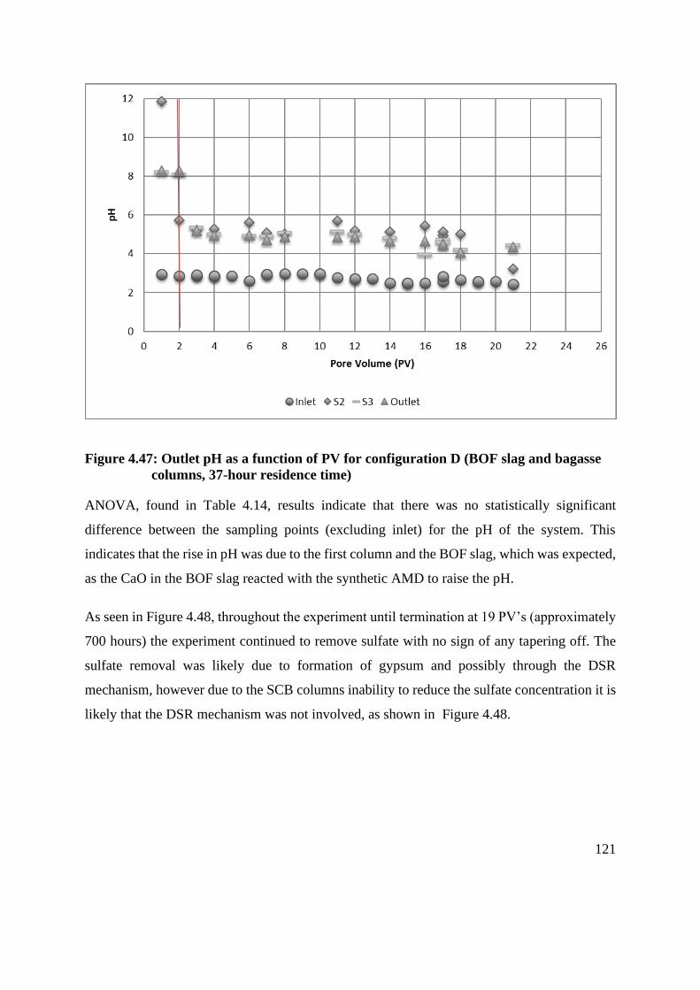
121



ANOVA, found in Table 4.14, results indicate that there was no statistically significant

difference between the sampling points (excluding inlet) for the pH of the system. This

indicates that the rise in pH was due to the first column and the BOF slag, which was expected,

as the CaO in the BOF slag reacted with the synthetic AMD to raise the pH.

As seen in Figure 4.48, throughout the experiment until termination at 19 PV’s (approximately

700 hours) the experiment continued to remove sulfate with no sign of any tapering off. The

sulfate removal was likely due to formation of gypsum and possibly through the DSR

mechanism, however due to the SCB columns inability to reduce the sulfate concentration it is

likely that the DSR mechanism was not involved, as shown in Figure 4.48.

122

Figure 4.48: Sulfate concentration as a function of PV for configuration D (BOF slag


The difference between sampling points S2, S3 and the outlet was not significant in terms of

sulfate concentration as indicated by ANOVA found in (Table 4.14) and this indicates that the

sulfate removal occurred in the first column of configuration D. This means that the sulfate

removal was through the formation of gypsum and that the second column did not remove

sulfate. The SRB in the second column may not have acclimated due to the initially high pH

(Figure 4.47) and it is also possible that the first column removed almost the maximum level

of sulfate for the system, thus not allowing the second column to remove as much sulfate as

initially expected and as discussed by Thauer and Kunow (1995) and Zhang et al. (2013), this

pH is not in a range in which the SRB tend to grow.

123

Figure 4.49: Percentage Sulfate removed as a function of PV for configuration D (BOF

slag and bagasse columns, 37-hour residence time)

Figure 4.49 gives the percentage sulfate removed with respect to PV at various sampling points.

The highest sulfate removed was at 17 PV’s with a high of 51%, before the sulfate removal

dropped slightly and the experiment was stopped. The value at the 1st PV was due to dilution

effects, as can be seen throughout the experiment where the measured concentration was

affected by the dilution done before measurement.

Figure 4.50 shows the concentration of dissolved iron with respect to PV at various sampling

points for a 37-hour residence time, the Fd was below 50 for the majority of the experiment,

except for the PV of 6 where the iron concentration rises above 50, this point could be due to

dilution effects, as the pH (Figure 4.47) is still above 5 at this point. The concentration of iron

in the sampling point’s increases above 50 at a PV of 19 for the Outlet and S3 sampling points.

124

Figure 4.50: Dissolved Iron concentration as a function of PV for configuration D (BOF


ANOVA (Table 4.14) results show that there was no statistically significant difference between

any of the data points from the sampling points in the system (inlet excluded), indicating that

the majority of iron removal occurs in the first column, which was expected as this was the

BOF slag column- column 1 (S2).

As seen in Figure 4.51 the percentage of dissolved iron removed had a high of 97.2% at a PV

of 2 and slowly lowers as the pH, as shown in Figure 4.47, decreases. The Fd removed

percentage reached a low of 90% at 19 PV’s, as potential depletion and/or armouring of the

BOF slag had occurred. The 19th PV coincides with a low pH, a pH below 5 and this shows a

correlation between pH and iron.

125

Figure 4.51: Percentage Dissolved Iron removed as a function of PV for configuration D

(BOF slag and bagasse columns, 37-hour residence time)

Figure 4.52 shows a 1000 times magnification image of BOF slag that had not been exposed

to AMD. The surface of the image appears to be relatively smooth when compared to Figure

4.53, which shows a 1000 times magnification image of BOF slag that had been exposed to

AMD. The EDX measured the iron on the surface of the unused slag, this came to a weight

percentage of 14.38 as seen below in Table 4.13. The 500X magnification may be seen in

Appendix B.

126


Figure 4.53: SEM results for configuration D, used BOF slag, 1000 X magnification

The EDX measured the iron on the surface of the BOF slag for configuration D, this came to a

weight of 40.05% indicating armouring of iron on the BOF slag. When images from Figure

4.52 and Figure 4.53 are compared it appears that the slag had undergone a change on the

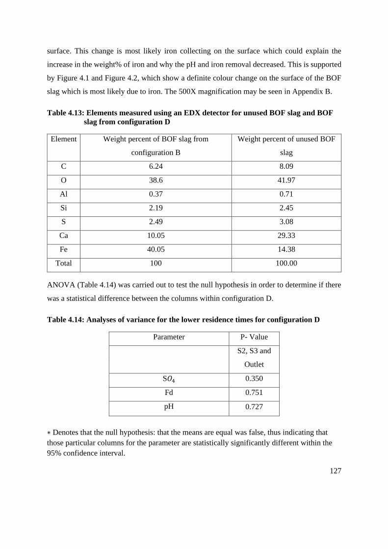
127

surface. This change is most likely iron collecting on the surface which could explain the

increase in the weight% of iron and why the pH and iron removal decreased. This is supported

by Figure 4.1 and Figure 4.2, which show a definite colour change on the surface of the BOF

slag which is most likely due to iron. The 500X magnification may be seen in Appendix B.


slag from configuration D

Element Weight percent of BOF slag from

configuration B

Weight percent of unused BOF

slag

C 6.24 8.09

O 38.6 41.97

Al 0.37 0.71

Si 2.19 2.45

S 2.49 3.08

Ca 10.05 29.33

Fe 40.05 14.38

Total 100 100.00

ANOVA (Table 4.14) was carried out to test the null hypothesis in order to determine if there

was a statistical difference between the columns within configuration D.

Table 4.14: Analyses of variance for the lower residence times for configuration D

Parameter P- Value

S2, S3 and

Outlet

S𝑂4 0.350

Fd 0.751

pH 0.727




128

The ANOVA results for configuration D show that there was no statistically significant

difference between the data (inlet excluded) for the sampling points for configuration D. This

means that after column one no significant treatment was taking place, indicating that the

sulfate and iron removal was in column 1 and that the rise in pH was in column 1. This could

be due to the placement of the BOF slag column, as this column was the first point of treatment

and the subsequent SCB column may not have been able to remove a significant amount of the

substances. Another possibility is that column 2 was not functional as the pH that entered into

this column was too high for the SRB as also discussed by Zhang et al. (2013) and Thauer and

Kunow (1995).

4.6.2 Treatment of acid mine drainage at low flow in configuration D (τ = 86

hours)

Figure 4.54 shows the pH of the inlet and the sampling points with respect to PV. In this

experiment the flow was low and thus there was more time for the lime to leach into the AMD

and assuming the SRB were functional there was then more time for the SRB to acclimate, thus

the pH increasing capacity was higher and lasted longer than in the high flow experiment

(Figure 4.47). The vertical line on the graph indicates that any potential to increase the pH was

depleted at this point. The high pH of 12.82 was indicative that the slag can raise the pH of a

synthetic AMD over 12 as was also shown by Name and Sheridan (2014). The BOF slag then

starts to show signs of depletion at a PV of 50. This was potentially due to armouring and

depletion of the slag.

129



The pH between the columns was not statistically significantly different as shown by the

ANOVA results (Table 4.14). It was clear from Figure 4.54 that the first column with BOF slag

raised the pH to approximately 12 and the second column with bagasse does not have an impact

on the pH, as was expected.


various sampling points with respect to PV. The AMD feed was changed at certain points

throughout the experiment, which appears to have impacted on the sulfate concentration in the

sampling points for this configuration. This does not seem to impact the other configurations

as much and could be due to the higher residence time in this configuration when compared to

other configurations. This impact can be seen at PV’s of 30 and 42 in Figure 4.55.

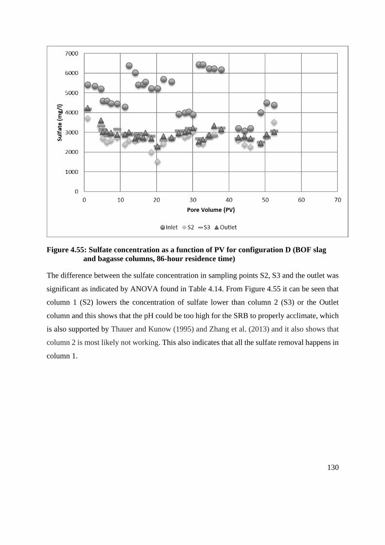
130

Figure 4.55: Sulfate concentration as a function of PV for configuration D (BOF slag



significant as indicated by ANOVA found in Table 4.14. From Figure 4.55 it can be seen that

column 1 (S2) lowers the concentration of sulfate lower than column 2 (S3) or the Outlet

column and this shows that the pH could be too high for the SRB to properly acclimate, which

is also supported by Thauer and Kunow (1995) and Zhang et al. (2013) and it also shows that

column 2 is most likely not working. This also indicates that all the sulfate removal happens in

column 1.

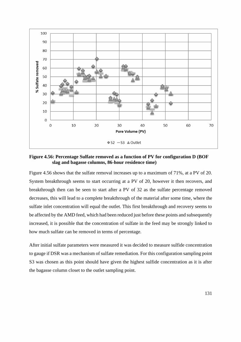
131

Figure 4.56: Percentage Sulfate removed as a function of PV for configuration D (BOF


Figure 4.56 shows that the sulfate removal increases up to a maximum of 71%, at a PV of 20.

System breakthrough seems to start occurring at a PV of 20, however it then recovers, and

breakthrough then can be seen to start after a PV of 32 as the sulfate percentage removed

decreases, this will lead to a complete breakthrough of the material after some time, where the

sulfate inlet concentration will equal the outlet. This first breakthrough and recovery seems to

be affected by the AMD feed, which had been reduced just before these points and subsequently

increased, it is possible that the concentration of sulfate in the feed may be strongly linked to

how much sulfate can be removed in terms of percentage.

After initial sulfate parameters were measured it was decided to measure sulfide concentration

to gauge if DSR was a mechanism of sulfate remediation. For this configuration sampling point

S3 was chosen as this point should have given the highest sulfide concentration as it is after

the bagasse column closet to the outlet sampling point.

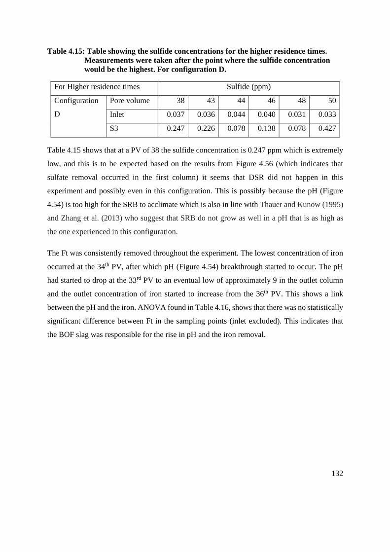
132



would be the highest. For configuration D.

For Higher residence times Sulfide (ppm)

Configuration

D

Pore volume 38 43 44 46 48 50

Inlet 0.037 0.036 0.044 0.040 0.031 0.033

S3 0.247 0.226 0.078 0.138 0.078 0.427

Table 4.15 shows that at a PV of 38 the sulfide concentration is 0.247 ppm which is extremely

low, and this is to be expected based on the results from Figure 4.56 (which indicates that

sulfate removal occurred in the first column) it seems that DSR did not happen in this

experiment and possibly even in this configuration. This is possibly because the pH (Figure

4.54) is too high for the SRB to acclimate which is also in line with Thauer and Kunow (1995)

and Zhang et al. (2013) who suggest that SRB do not grow as well in a pH that is as high as

the one experienced in this configuration.

The Ft was consistently removed throughout the experiment. The lowest concentration of iron

occurred at the 34th PV, after which pH (Figure 4.54) breakthrough started to occur. The pH

had started to drop at the 33rd PV to an eventual low of approximately 9 in the outlet column

and the outlet concentration of iron started to increase from the 36th PV. This shows a link

between the pH and the iron. ANOVA found in Table 4.16, shows that there was no statistically

significant difference between Ft in the sampling points (inlet excluded). This indicates that

the BOF slag was responsible for the rise in pH and the iron removal.

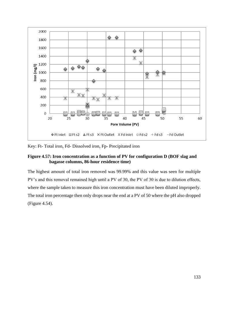
133


Figure 4.57: Iron concentration as a function of PV for configuration D (BOF slag and


The highest amount of total iron removed was 99.99% and this value was seen for multiple

PV’s and this removal remained high until a PV of 30, the PV of 30 is due to dilution effects,

where the sample taken to measure this iron concentration must have been diluted improperly.

The total iron percentage then only drops near the end at a PV of 50 where the pH also dropped

(Figure 4.54).

134

Key: Ft- Total iron

Figure 4.58: Percentage Total Iron removed as a function of PV for configuration D

(BOF slag and bagasse columns, 86-hour residence time)

The calcium as shown in Figure 4.59 reached a high of 886 ppm at the 34th PV and slowly

decreased as the calcium was depleted to a low of 161 ppm at 50 PV’s. This depletion shows

that the BOF slag was leaching calcium into the AMD as CaO, which was raising the pH and

was why there was a drop in pH (Figure 4.54) to approximately 6, when the calcium

concentration starts to drop.

This shows a link between the pH and the calcium. With regards to calcium the ANOVA (Table

4.16) test showed that there was no statistical significant difference between the columns (inlet

excluded), because the BOF slag was the predominant cause for calcium in the system and the

BOF slag was in the first column.

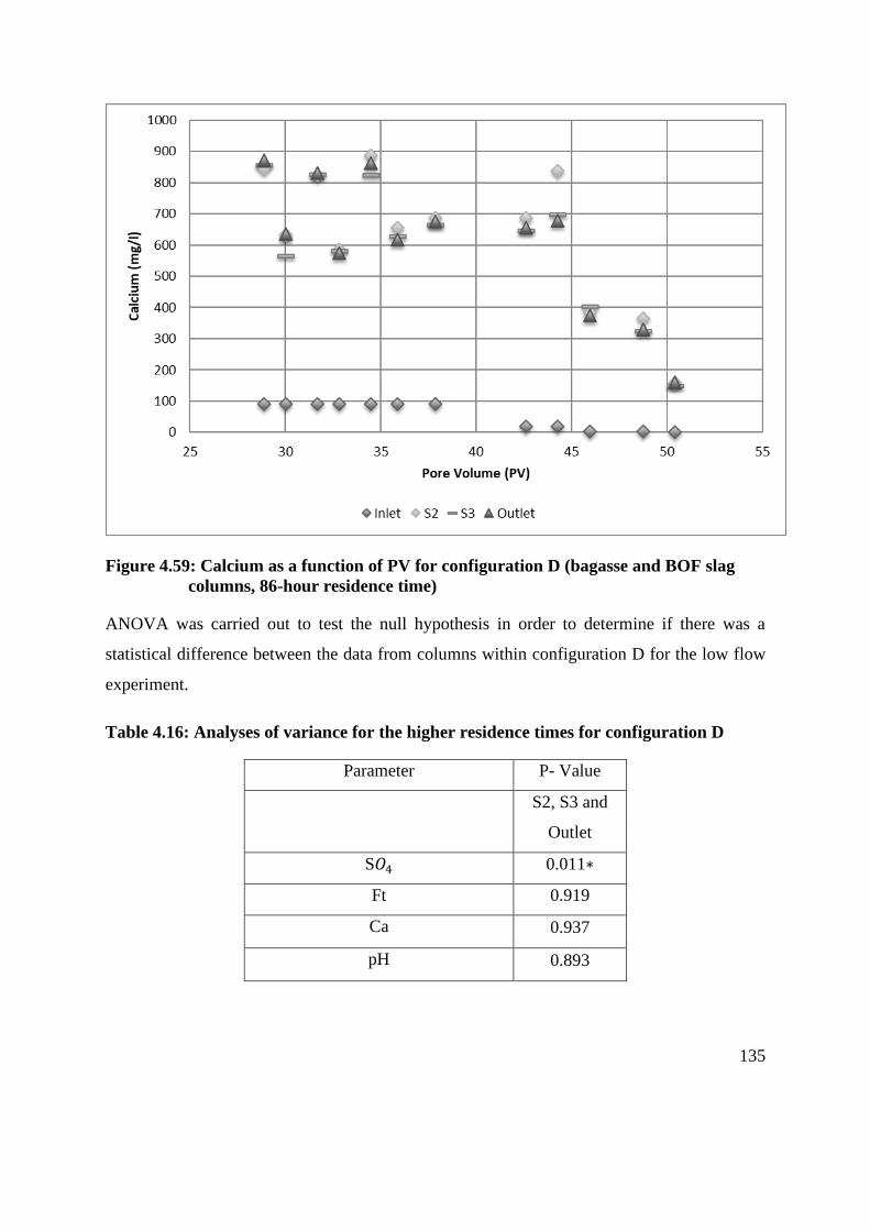
135

Figure 4.59: Calcium as a function of PV for configuration D (bagasse and BOF slag



statistical difference between the data from columns within configuration D for the low flow

experiment.

Table 4.16: Analyses of variance for the higher residence times for configuration D

Parameter P- Value

S2, S3 and

Outlet

S𝑂4 0.011∗

Ft 0.919

Ca 0.937

pH 0.893

136




The ANOVA results (Table 4.16) for configuration D show that there was a statistically

significant difference for the data between the columns for sulfate in configuration D. This

indicates as can be seen in Figure 4.55, that there was a difference between the columns when

it comes to removing the sulfate, and that column 1 containing the BOF slag was responsible

for the sulfate removal.


configuration D

The very high flow experiment for configuration D shows that the pH increased to a pH of 8

and maintained this level for approximately 85 hours where it then started to decrease; this is

not effective as the pH starts to decrease too quickly relative to the low and high flow, and if

the pH cannot be maintained treatment will not last long enough to allow the removal of heavy

metals. This is possibly due to the volume of AMD that is passing through the column and the

amount of iron that was subsequently most likely armouring the BOF slag. If the high flow and

low flow experiments are compared an increase in pH may be observed with an increase in

residence time, which indicates as the contact time between the BOF slag and SCB increased

the pH increased. Similar trends may be seen for the other parameters in relation to residence

time.

Comparing the low flow and high flow experiments it can be seen that more sulfate and iron is

removed for a longer period of time as the residence time is increased, a higher pH is also

reached and maintained for a longer period with a higher residence time. This experiment along

with the other experiments indicates that residence time is very important when considering

sulfate and iron removal and pH increase. Both the low flow and high flow experiments also

indicated that column 1 was responsible for the removal of the sulfate and iron and this may

have been as a result of the pH entering into column 2 which was not favourable for SRB

growth.

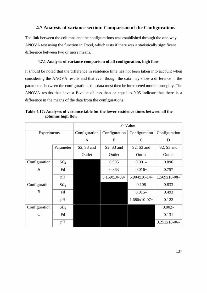
137

4.7 Analysis of variance section: Comparison of the Configurations

The link between the columns and the configurations was established through the one-way

ANOVA test using the function in Excel, which tests if there was a statistically significant

difference between two or more means.

4.7.1 Analysis of variance comparison of all configuration, high flow

It should be noted that the difference in residence time has not been taken into account when

considering the ANOVA results and that even though the data may show a difference in the

parameters between the configurations this data must then be interpreted more thoroughly. The

ANOVA results that have a P-value of less than or equal to 0.05 indicate that there is a

difference in the means of the data from the configurations.

Table 4.17: Analyses of variance table for the lower residence times between all the

columns high flow

P- Value

Experiments Configuration

A

Configuration

B

Configuration

C

Configuration

D

Parameter S2, S3 and

Outlet

S2, S3 and

Outlet

S2, S3 and

Outlet

S2, S3 and

Outlet

Configuration

A

S𝑂4 0.995 0.001∗ 0.896

Fd 0.363 0.016∗ 0.757

pH 5.169x10-09∗ 6.904x10-14∗ 1.569x10-08∗

Configuration

B

S𝑂4

0.108 0.833

Fd 0.015∗ 0.493

pH 1.680x10-07∗ 0.122

Configuration

C

S𝑂4

0.002∗

Fd 0.131

pH 3.251x10-06∗

138

∗ Denotes that the null hypothesis: that the means are equal was false, thus indicating that those particular columns

for the parameter are statistically significantly different within the 95% confidence interval. The blacked-out areas

represent the ANOVA results that have already been shown and discussed or areas that aren’t relevant.

The ANOVA results for configuration A when compared with configuration B, show that there

was a statistically significant difference between the pH of A and B. The results as seen in

Figure 4.6 and Figure 4.18 show that for a low pH stream of AMD the layout of configuration

B should be used to treat the AMD, even though ANOVA doesn’t specify this, from the pH

graphs it can be determined.

The ANOVA results for configuration A when compared with configuration C, show that there

was a statistically significant difference in all three parameters. These results together with the

graphs shown in Figure 4.7, Figure 4.8, Figure 4.12 and Figure 4.13, indicate that if a user

wanted the lowest sulfate concentration in the treated AMD between these configurations,

configuration A would be the appropriate configuration. If the user wanted the pH of the AMD

to rise the highest out of these configurations, configuration C would be the most appropriate

and for the highest dissolved iron percentage removed, configuration C again would be the

most appropriate configuration, which is to be expected as configuration C had BOF slag in

the columns.

The ANOVA results for configuration A when compared to configuration D, show that the

only statistically significant difference between the columns was the pH. The graphs shown in

Figure 4.6 and Figure 4.47 show that a low pH stream of AMD would best be suited for

configuration D, as configuration D raised the pH the highest out of the two configurations.

The ANOVA results for configuration B when compared to configuration C show that there

was a statistically significant difference between pH and Fd. Figure 4.18, Figure 4.21, Figure

4.32 and Figure 4.35 in the results section show that configuration C raises the pH and removes

more dissolved iron than configuration B, leading to the conclusion that configuration C (which

has a higher residence time) would treat synthetic AMD significantly better than configuration

B (which has a lower residence time) in terms of dissolved iron removed and a rise in pH.

139

The ANOVA results for configuration B when compared with configuration D show that there

was no statistically significant difference, indicating that neither configuration performs

statistically better than the other.

The ANOVA results for configuration C when compared with configuration D show that there

was a statistically significant difference between the sulfate and the pH. Figure 4.32, Figure

4.33, Figure 4.47 and Figure 4.48 show that configuration C was better for a sustained higher

pH (in the outlet) while configuration D will be more suited than configuration C in removing

sulfate.

4.7.2 Analysis of variance comparison of all configuration, low flow

It should be noted that the difference in residence time has not been taken into account when

considering the ANOVA results and that as residence time is considered the results from

ANOVA can still be used but must be used with the knowledge of the difference in residence

time.

The ANOVA results for configuration A when compared with configuration B, show that there

was a statistically significant difference between the pH, total iron and calcium of

configurations A and B. These results show that if the goal is to raise the pH the highest and

remove the most amount of iron configuration B should be used, even though the ANOVA

doesn’t specify this, from the pH and iron graphs shown in Figure 4.6, Figure 4.9 , Figure 4.25

and Figure 4.28 it can be determined. The calcium results are as expected as the BOF slag

material was only found in configuration B and as previously discussed the CaO in the BOF

slag increased the calcium concentration which caused a difference between the two

configurations in relation to calcium.

140

Table 4.18: Analyses of variance table for the higher residence times between all the

columns for low flow

P-Value

Experiments Configuration

A

Configuration

B

Configuration

C

Configuration

D

Parameter S2, S3 and

Outlet

S2, S3 and

Outlet

S2, S3 and

Outlet

S2, S3 and

Outlet

Configuration

A

S𝑂4 0.999 0.531 0.390

Ft 5.79x10-12∗ 1.2x10-10∗ 0∗

Ca 2.03x10-13∗ 0∗ 1.37x10-14∗

pH 0∗ 0∗ 0∗

Configuration

B

S𝑂4

0,396 0.219

Ft 1.259x10-05∗ 1.080x10-10∗

Ca 0.005∗ 0.059

pH 0∗ 0∗

Configuration

C

S𝑂4

0.199

Ft 0.067

Ca 0.658

pH 0∗

∗ Denotes that the null hypotheses: that the means are equal was false, thus indicating that those particular

columns for the parameter are statistically significantly different within the 95% confidence interval.

The ANOVA results for configuration A when compared with configuration C show that

there was a statistically significant difference between the pH, total iron and calcium of

configurations A and C. These result show that a low pH stream of AMD with a high iron

content would be better suited using the layout of configuration C, which can be determined

from the pH and iron graphs shown in Figure 4.6,, Figure 4.14 Figure 4.40 and Figure 4.43.

The calcium results are as expected as the BOF slag that was only in configuration C, will

cause a difference between the two configurations calculated means in terms of calcium.

The ANOVA results for configuration A when compared with configuration D show that

there was a statistically significant difference between the pH, total iron and calcium. These

141

result show that if the goal is to achieve a higher iron percentage removal and a higher rise in

pH then configuration D should be used, even though the ANOVA doesn’t specify this, from

the pH and iron graphs in Figure 4.6, Figure 4.14, Figure 4.54 and Figure 4.57 it can be

determined. The difference in calcium is expected as only configuration D had the BOF slag

material, which leached CaO into the synthetic AMD and raised the pH.

The ANOVA results for configuration B when compared to configuration C show that there

was a statistically significant difference between the pH, total iron and calcium. These results

show that a low pH stream of AMD with a high iron concentration would be better treated

using configuration B’s setup, even though the ANOVA doesn’t specify this, from the pH

graphs shown in Figures Figure 4.25 and Figure 4.40 it can be determined. The ANOVA results

show that the iron in configurations B and C differ, this difference, by considering the graphs

found in Figure 4.28 and Figure 4.43, can be explained as the difference in iron removal

between the SCB column in configuration B (column 1) and the BOF slag and SCB column

mixture in configuration C (column 1). The SCB and BOF slag column mixture in

configuration C performs better than SCB column in B, possibly due to the pH, as the pH in

configuration C column 1 was at a better value for the SRB to grow according to Zhang et al.

(2013) and Thauer and Kunow (1995); where the pH growth (depending on the genesis) is

hypothesized to best grow at a pH of 5.5-7.5. The difference in calcium as shown by the

ANOVA results can be explained by the different materials in the columns for the respective

configurations as shown in Figure 4.30 and Figure 4.45, the fact that calcium was leaching into

the synthetic AMD from the first column in configuration C and only from the second column

in configuration B meant that the difference was expected.

The ANOVA results for configuration B when compared to configuration D show that there

was a statistically significant difference between total iron and pH. The results show that a low

pH stream of AMD with a high iron content would be better suited using the layout of

configuration D, even though the ANOVA doesn’t specify this, from the pH and iron graphs

shown in Sections 4.2.2, 4.2.5, 4.5.1 and 4.5.4 it can be determined.

142

The ANOVA results for configuration C when compared to configuration D show that there

was a statistically significant difference between pH. This result as seen in Figure 4.40 and

Figure 4.54 indicates that if a high pH is wanted in the outlet of a stream of AMD, configuration

D should be used.

4.8 Comparison of best results considering residence times

The different residence times are important to consider, and the Table 4.19 shows the residence

time and maximum percentage removed for each configuration, as well as where breakthrough

starts to occur for pH. The results do give an indication as to which configuration performs

most effectively for removing sulfate, iron and raising the pH, however a more in-depth review

of the results is given in Table 4.19.

Table 4.19: Table for all configurations and the maximum removal for sulfate and iron

and the highest pH

Residence

time

(hr/𝑚𝑙2)

%

Maximum

Sulfate

removed

%

Maximum

Iron

removed

Maximum

pH when

inlet was

below 3

PV at which

breakthrough

starts to

occur for pH

Configuration A 34 58 92(Fd) 5.08 14

83 86 90 (Ft) 5.86 21

Configuration B 30 54 94(Fd) 10.31 2

71 67 99.9(Ft) 12.79 55

Configuration C 41 41 99.6(Fd) 12.27 3 and 11

79 73 99.7(Ft) 12.82 10 and 20

Configuration D 37 51 97.2(Fd) 11.85 2

86 71 99.99(Ft) 12.82 50

The configuration that achieves the highest iron percentage removal and raises the pH the

highest was configuration D and had the highest sulfate percentage removal over all the

configurations with BOF slag, with consistency over the two residence times. This

configuration had the best performance with the highest residence time, which was expected,

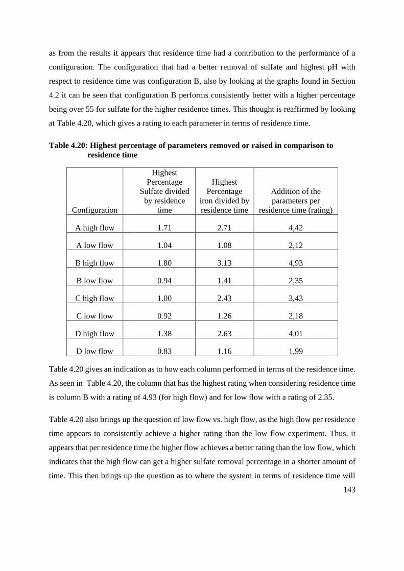
143

as from the results it appears that residence time had a contribution to the performance of a

configuration. The configuration that had a better removal of sulfate and highest pH with

respect to residence time was configuration B, also by looking at the graphs found in Section

4.2 it can be seen that configuration B performs consistently better with a higher percentage

being over 55 for sulfate for the higher residence times. This thought is reaffirmed by looking

at Table 4.20, which gives a rating to each parameter in terms of residence time.

Table 4.20: Highest percentage of parameters removed or raised in comparison to

residence time

Configuration

Highest

Percentage

Sulfate divided

by residence

time

Highest

Percentage

iron divided by

residence time

Addition of the

parameters per

residence time (rating)

A high flow 1.71 2.71 4,42

A low flow 1.04 1.08 2,12

B high flow 1.80 3.13 4,93

B low flow 0.94 1.41 2,35

C high flow 1.00 2.43 3,43

C low flow 0.92 1.26 2,18

D high flow 1.38 2.63 4,01

D low flow 0.83 1.16 1,99

Table 4.20 gives an indication as to how each column performed in terms of the residence time.

As seen in Table 4.20, the column that has the highest rating when considering residence time

is column B with a rating of 4.93 (for high flow) and for low flow with a rating of 2.35.

Table 4.20 also brings up the question of low flow vs. high flow, as the high flow per residence

time appears to consistently achieve a higher rating than the low flow experiment. Thus, it

appears that per residence time the higher flow achieves a better rating than the low flow, which

indicates that the high flow can get a higher sulfate removal percentage in a shorter amount of

time. This then brings up the question as to where the system in terms of residence time will

144

reach an asymptote in terms of the sulfate and iron removal. It should also be noted that Table

4.20 is only looking at the highest percentage removed and not how long a specific percentage

was maintained, as shown in previous sections the low flow experiments experience

breakthrough at a later point in time than the high flow experiments in terms of pH.

145

5 Discussion and conclusion

The ultimate goals of this research was to determine if a combination of the SCB and BOF slag

could remediate synthetic AMD, if it was possible to remediate the synthetic AMD to a level

which would be acceptable for crop irrigation (Table 2.8) and which configuration would be

the most effective in the treatment. The results showed the combination of BOF slag and SCB

was effective at significantly raising the pH of highly acidic AMD, removing total and

dissolved iron and removing sulfate at residence times of 35.5 hours ± 5.5 and 78.5 hours ±

7.5. The result for the configuration that had two SCB columns in a row (configuration A)

showed that the material was able to remove sulfate and iron and raise the pH slightly in the

high flow experiment and raise the pH to near neutral conditions as well as remove iron and

sulfate in the low flow experiment for a period of time that was less than the configurations

containing BOF slag.

The results showed that as the residence time increased the percentage removal of sulfate, and

iron also increased, and the pH was raised higher for a longer period of time. For configuration

A the pH for the low flow experiment reached a high of 5.86 when the inlet pH was 2.75, whilst

the high flow experiment reached a high of 5.08 for an inlet pH of 2.85, and the low flow

experiment removed 86% of the sulfate whilst the high flow experiment removed 58%. These

results indicate the higher potential for a longer residence time for configuration A and this

becomes a pattern for the other configurations as shown in the Table 4.19.

Table 4.19 also shows that configuration D removed the most amount of sulfate, iron (total and

dissolved) and raised the pH the highest over the two experiments on average, however this

configuration also had the highest residence times. Considering residence times and by looking

at the results in Section 4.2 and Table 4.20 it appears that the column that removed the most

sulfate, iron and raised the pH the highest with a lower residence time on average over the two

experiments was configuration B. Configuration C also has a higher removal percentage of

sulfate and iron and raised the pH more on average over the three parameters than configuration

D for the low flow experiments when considering residence time. The ANOVA results give an

146

indication that the columns with BOF slag were statistically significantly different to the

columns without BOF slag.

The ANOVA results indicate that having BOF slags in the configuration provides a statistically

significant rise in the pH of the system and for the higher residence times also provides a

statistically significant difference in total iron and calcium. It is also evident for configurations

containing slag that pH breakthrough occurs much later. The breakthrough curves were also

established and for the high flow experiments a breakthrough was found early on for the pH’s

of the varying systems but for the low flow experiments a breakthrough only happened in most

cases at a PV of around 50. The breakthrough for configuration A occurred later on for the pH

in the low flow experiments but both occurred earlier than any other system. This can be

explained by the absence of BOF slag. Armouring may also have been a factor in the

breakthrough curves for the pH of the systems, containing BOF slag.

Potential armouring as shown in the SEM images, supported by the EDX results (which, show

an increase in the iron weight percentage on the surface of the BOF slag) and Figure 4.1 and

Figure 4.2 show an increase of iron on the surface which is most likely the cause of the start of

the breakthrough of the pH. This drop in pH was also due potentially to depletion of the calcium

in the BOF slags as shown in the calcium figures for the low flow experiments. The results

from the experiments conducted give an indication as to what the combination of these systems

can achieve when it comes to AMD remediation; the knowledge of this treatment system does

need to be broadened to understand the systems better.

The systems with the BOF slag cannot be applied to all AMD, as an AMD with a higher pH

bordering on 5 does not necessarily need a big pH increase because a pH of 5 is generally

considered acceptable. The systems with BOF slag may also not be the most suitable as they

are currently set up, as achieving a pH above 9 is not necessarily a good pH and is not the best

conditions for the SRB according to Zhang et al. (2013). A possible set up where the slag only

increases the pH of the AMD to about 7 or 8 may be the better solution, as this will still

precipitate out most heavy metals and will allow the next phase of the treatment with SRB to

work more effectively. A system that is set up with the slag first to raise a low pH AMD stream

to a pH over 12, which will then be combined with another low pH AMD stream in order to

147

get both AMD streams pH’s to roughly 7. This new stream of AMD with a pH of 7 can then

be entered into the SCB column; this could be a more effective treatment system as it will allow

the SRB to acclimate more effectively. The SCB and BOF slag that has been produced in South

Africa may also not necessarily have the same properties in other countries and the experiment

thus far can only safely determine that the systems work as they do with the combination SCB

and BOF slags attained from UCL and attained from SCAW metals respectively. Without the

knowledge that the material performs in the same way at different places and in different

conditions, the systems cannot be said to remediate AMD throughout the world but only with

the materials and conditions used in this experiment. The system while remediating synthetic

AMD may also not perform in the same way when using AMD that has not been modelled in

a lab. Another drawback in this experiment was the lack of experimental data to determine the

neutralization of acidity for BOF slag this is complex due to the composition of the slag being

composed of several alkaline components. This experiment should be conducted by any future

users. The acidity of the synthetic AMD for future experiments should also be quantified as the

more complex a solution the more chances there are of forming complexes in solution.

Whilst the crop irrigation limits were the ones considered this must still be done with the source

of the AMD in mind. If the AMD source has low levels of iron and sulfate it is possible that

using the combination of SCB and BOF slag could reduce the iron and sulfate levels to those

of drinking standards or sewage discharge standards or any other standard as shown in Table

2.8. The research on this was not done and as such further research where the sulfate and iron

levels in the AMD are not as high must be done in order to asses if these parameters can be

reduced to fall into the permissible limits of other discharge limits. It is also important to

research the percentage reduced of the iron and sulfate concentrations in terms of different

starting iron and sulfate concentrations; is it exponential or linear or possibly some other

correlation? This will allow someone who uses the SCB and BOF slag combination to treat

AMD to decide the end result more efficiently (to what levels do they want to remove the

sulfate and iron). It is also highly recommended that research into a material balance be

completed, this will allow a pinpoint determination of the iron removal. If the iron removal is

all being attributed to FeS formation then the material balance should confirm the iron to sulfide

ratio, however this dissertation does not attribute all the iron removal in the columns to

148

biological activity. There should also have been control experiments DSR on SCB as the carbon

source. The control experiment should have many controls put in place, with one of them being

low pH.

The research objectives were to study the influence of the residence times on the

configurations, determine the breakthrough time of the species and to study the physical and

chemical changes of the BOF slag before and after treatment.

The results indicated that the low flow experiment removed more sulfate and iron and

maintained this removal for longer periods and raised the pH higher. The low flow experiments

did not reach a point where the high flow experiments were removing more sulfate or iron or

raising the pH higher thus there does not appear to be a limit to residence time in terms of

remediation potential; however this will need to be researched further in order to determine if

there is a low flow experiment which does not remove sulfate and iron to a higher value than

the previous high flow experiment.

When residence time is taken into account the configuration that remediated the most was

Configuration B with a residence time of 71-hours and breakthrough occurred at PV of 55

where the pH failed to get above 6.6, which indicates that the BOF slag needs to be replaced.

The physical and chemical changes of the BOF slag before and after treatment were determined

for the lower residence time and it was determined that armouring had occurred, this was

supported by the results of the EDX detector results which showed a large gain in mass

percentage of iron on the surface of the BOF slag and was also supported by Figure 4.1 and

Figure 4.2, which showed a clear colour change on the surface of the BOF slag which was true

for all columns containing BOF slag.

149

Reference

Advisory, D.W., 2003. Consumer acceptability advice and health effects

analysis on sodium. US Environmental Protection Agency Office of Water

(4304T), Health and Ecological Criteria Division, Washington, DC, 20460.

Aguinaga, O.E., Wakelin, J.F., White, K.N., Dean, A.P. and Pittman, J.K.,

2019. The association of microbial activity with Fe, S and trace element

distribution in sediment cores within a natural wetland polluted by acid mine

drainage. Chemosphere, 231, pp.432-441.

Akcil, A. and Koldas, S., 2006. Acid Mine Drainage (AMD): causes, treatment

and case studies. Journal of Cleaner Production, 14(12-13), pp.1139-1145.

Akpor, O.B. and Muchie, M., 2010. Remediation of heavy metals in drinking

water and wastewater treatment systems: Processes and applications.

International Journal of Physical Sciences, 5(12), pp.1807-1817.

Alexiou, I.E. and Panter, K., 2004, September. A review of two-phase

applications to define best practice for the treatment of various waste streams.

In Anaerobic Digestion 10th World Congress, Sept 2004. Montreal, Quebec,

Canada.

Alves, E.F., Bose, S.K., Francis, R.C., Colodette, J.L., Iakovlev, M. and Van

150

Heiningen, A., 2010. Carbohydrate composition of eucalyptus, bagasse and

bamboo by a combination of methods. Carbohydrate Polymers, 82(4),

pp.1097-1101.

Anukam, A., Mamphweli, S., Meyer, E. and Okoh, O., 2013. Gasification of

sugarcane bagasse as an efficient conversion technology for the purpose of

electricity generation. Fort Hare Papers. Multidiscip J University Fort Hare,

20(1).

Aubé, B., Zinck, J. and Eng, M., 2003, December. Lime treatment of acid mine

drainage in Canada. In Brazil-Canada Seminar on Mine Rehabilitation (pp. 23-

39). Florianopolis: Desktop Publishing.

Aydilek, A.H. and Dayioglu, A.Y., 2015. Geotechnical and environmental

impacts of steel slag use in highway construction. University of Maryland,

Final report.

Ball, J.W. and Nordstrom, O.K., 1991, WATEQ4F User's manual with revised

thermodynamic data base and test cases for calculating speciation of major,

trace and redox elements in natural waters: U.S. Geological Survey Open-File

Report 90-129, p.185.

Banks, D., Younger, P.L., Arnesen, R.T., Iversen, E.R. and Banks, S.B., 1997.

Mine-water chemistry: the good, the bad and the ugly. Environmental

Geology, 32(3), pp.157-174.

151

Barakat, M.A., 2011. New trends in removing heavy metals from industrial

wastewater. Arabian journal of chemistry, 4(4), pp.361-377.

Bowden, L.I., Johnson, K.L., Jarvis, A.P., Robinson, H., Ghazireh, N. and

Younger, P.L., 2006, March. The use of basic oxygen steel furnace slag (BOS)

as a high surface area media for the removal of iron from circum neutral mine

waters. In Proceedings of the 7th International Conference on Acid Rock

Drainage (ICARD), St. Louis, Missouri, USA (pp. 26-30).

Bowell, R.J. 2004. A review of sulphate removal options for mine waters. In:

Jarvis, A.P., Dudgeon, B.A. and Younger, P.L (eds) Proceedings of the

Symposium: Mine Water 2004- Process, Policy and Progress, Volume 2.

University of Newcastle, New castle upon Tyne, UK, 19-23 September.

Brady, K.S., Bigham, J.M., Jaynes, W.F. and Logan, T.J., 1986. Influence of

sulfate on Fe- oxide formation: Comparisons with a stream receiving acid mine

drainage. Clays and Clay Minerals, 34(3), pp.266-274.

Canfield, D.E., Kristensen, E. and Thamdrup, B., 2005. Aquatic

Geomicrobiology. London: Elsevier. p.640 (Advances in Marine Biology; 48)

CDC (Centres for Disease Control) and USEPA (US Environmental Protection

Agency), 1999. Health Effects from Exposure to High Levels of Sulfate in

Drinking Water Study.

Available at:

152

https://www.who.int/water_sanitation_health/dwq/chemicals/sulfate.pdf

[Accessed 08 06 2016]

Cerqueira, D.A., Rodrigues Filho, G. and da Silva Meireles, C., 2007.

Optimization of sugarcane bagasse cellulose acetylation. Carbohydrate

Polymers, 69(3), pp.579-582.

Chapman, A., 2011. Acid mine drainage in South Africa: An Emerging

Environmental Problem. Institute for Futures Research, Stellensbosch

City of Johannesburg. 2008. Metropolitan Municipality Water Services

By-laws, published under notice no 835 in Gauteng Provincial Gazette

extraordinary no 179 dated 21 May 2004 and as amended by notice 1455 in

Provincial Gazette no 162 dated 20 June 2008.

Available at:

https://www.johannesburgwater.co.za/wp-content/uploads/2016/03/Water-Services-

Bylaws.pdf

[Accessed 08 06 2018]

Cline, J.D., 1969. Spectrophotometric determination of hydrogen sulfide in

natural waters 1. Limnology and Oceanography, 14(3), pp.454-458.

Coetzee, H., Hobbs, P.J., Burgess, J.E., Thomas, A., Keet, M., Yibas, B., Van

Tonder, D., Netili, F., Rust, V., Wade, P. and Maree, J., 2010. Mine water

management in the Witwatersrand Gold Fields with special emphasis on acid

https://www.who.int/water_sanitation_health/dwq/chemicals/sulfate.pdf

https://www.johannesburgwater.co.za/wp-content/uploads/2016/03/Water-Services-Bylaws.pdf

https://www.johannesburgwater.co.za/wp-content/uploads/2016/03/Water-Services-Bylaws.pdf

153

mine drainage. Report to the inter-ministerial committee on acid mine

drainage, pp.1-128.

Cravotta, C.A., 2003. Size and performance of anoxic limestone drains to

neutralize acidic mine drainage. Journal of Environmental Quality, 32(4),

pp.1277-1289.

Dauknys, R., Mažeikien, A., Haluza, A., Halauniou, I. and Yushchenko, V.,

2017. Preliminary Investigation of Primary Sludge Hydrolysis.

In Environmental Engineering. Proceedings of the International Conference on

Environmental Engineering. ICEE (Vol. 10, pp. 1-5). Vilnius Gediminas

Technical University, Department of Construction Economics & Property.

Department: Minerals and Energy, Republic of South Africa., 2003. A review of

the dolomite and limestone industry in South Africa. Directorate: Mineral

Economics. First Edition.

Available at:

https://www.dmr.gov.za/LinkClick.aspx?fileticket=gpszd6p3bqQ%3D&portalid=0

[Accessed 08 07 2019]

Department of water affairs and forestry (DWAF). 1996. South African, Water

Quality Guidelines (2nd Edition). Volumes 1–8. Pretoria.

Duruibe, J.O., Ogwuegbu, M.O.C. and Egwurugwu, J.N., 2007. Heavy metal

pollution and human biotoxic effects. International Journal of physical

sciences, 2(5), pp.112-118.

https://www.dmr.gov.za/LinkClick.aspx?fileticket=gpszd6p3bqQ%3D&portalid=0

154

Environmental, L., 2003. Treatment of sulphate in mine effluents. International

Network for Acid Prevention, Utah.

Epel, B., Schäfer, K.O., Quentmeier, A., Friedrich, C. and Lubitz, W., 2005.

Multifrequency EPR analysis of the dimanganese cluster of the putative sulfate

thiohydrolase SoxB of Paracoccus pantotrophus. Journal of Biological

Inorganic Chemistry, 10(6), pp.636-642.

US Environmental Protection Agency., 1983. Methods for chemical analysis

of water and wastes. EPA-600/4–79-020.USEPA (US Environmental

Protection Agency), Cincinnati, OH. Calcium: Method 215, 1(atomic

absorption, direct aspiration).

Euroslag, 2017. Basic oxygen furnace slag. The European

Association representing metallurgical slag producers and

processors, p.1.

Available at:

http://www.euroslag.com/products/bos/.

[Accessed 08 06 2018]

Feng, D., Van Deventer, J.S.J. and Aldrich, C., 2004. Removal of pollutants

from acid mine wastewater using metallurgical by-product slags. Separation

and purification technology, 40(1), pp.61-67.

http://www.euroslag.com/products/bos/

155

Foudhaili, T., Rakotonimaro, T.V., Neculita, C.M., Coudert, L. and Lefebvre,

O.P., 2019. Comparative efficiency of microbial fuel cells and

electrocoagulation for the treatment of iron-rich acid mine drainage. Journal of

Environmental Chemical Engineering, pp.103149.

Garribba, E., Micera, G., Panzanelli, A., Strinna-Erre, L. and Stara, G., 2001.

Distinguishing Calcium Carbonate from Calcium Sulfate Dihydrate by

Instrumental Methods. A Set of Laboratory Experiments for Analytical

Chemistry and Spectroscopy. Journal of Chemical Education, 78(8), p.1090.

Gaikwad, R.W. and Gupta, D.V., 2008. Review on removal of heavy metals

from acid mine drainage. Applied Ecology and Environmental Research, 6(3),

pp.81-98.

Gardea-Torresdey, J.L., Peralta-Videa, J.R., De La Rosa, G. and Parsons, J.G.,

2005. Phytoremediation of heavy metals and study of the metal coordination

by X-ray absorption spectroscopy. Coordination chemistry reviews, 249(17-

18), pp.1797-1810.

Garland, R., 2011. Acid mine drainage-can it affect human health?. Quest, 7(4),

pp.46-47.

Grewar, T., 2019. South Africa's options for mine-impacted water re-use: A

review. Journal of the Southern African Institute of Mining and Metallurgy,

119(3), pp.321-331.

156

Grubb, D.G., Landers, D.G., Guerra, P.A., Miller, B., Bilgin, A. and

Hernandez, M.T., 2018. Sugarcane Bagasse as a Microbial Host Media for the

Passive Treatment of Acid Mine Drainage. Journal of Environmental

Engineering, 144(10), p.04018108.

Harrison, S.T., 2014. Addressing the Challenges Facing Biological Sulphate

Reduction as a Strategy for AMD Treatment: Analysis of the Reactor Stage:

Raw Materials Products and Process Kinetics, Water Research Commission,

Pretoria, South Africa.

Hedin, R.S., Watzlaf, G.R. and Nairn, R.W., 1994. Passive treatment of acid

mine drainage with limestone. Journal of Environmental Quality, 23(6),

pp.1338-1345.

Järup, L., 2003. Hazards of heavy metal contamination. British medical bulletin,

68(1), pp.167- 182.

Jennings, S.R., Neuman, D.R. and Blicker, P.S., 2008. Acid mine drainage and

effects on fish health and ecology: A review. Reclamation Research Group

Publication, Bozeman, MT.

Ji, L., Yu, H., Yu, B., Jiang, K., Grigore, M., Wang, X., Zhao, S. and Li, K.,

2018. Integrated absorption–mineralisation for energy-efficient CO2

sequestration: Reaction mechanism and feasibility of using fly ash as a

157

feedstock. Chemical Engineering Journal, 352, pp.151-162.

Johnson, D.B. and Hallberg, K.B., 2003. The microbiology of acidic mine

waters. Research in microbiology, 154(7), pp.466-473.

Johnson, D.B. and Hallberg, K.B., 2002. Pitfalls of passive mine water

treatment. Reviews in Environmental Science and Biotechnology, 1(4),

pp.335-343.

Johnson, D.B. and Hallberg, K.B., 2005. Acid mine drainage remediation

options: a review. Science of the total environment, 338(1-2), pp.3-14.

Jones, R.T., 2004. Economic and environmentally beneficial treatment of slags

in DC arc furnaces. In proceedings of the VII international conference on

molten slags, fluxes and salts, The South African Institute of Mining and

Metallurgy, Cape Town, South Africa.

Kaksonen, A. H., & Sahinkaya, E., 2012. Review of sulfate reduction based

bioprocesses for acid mine drainage treatment and metals recovery. Paper

presented at the International Mine Water Association Annual Conference

(IMWA 2012), Bunbury, Western Australia.

Khayatzadeh, J. and Abbasi, E., 2010. The effects of heavy metals on aquatic

animals. In The 1st International Applied Geological Congress, Department of

158

Geology, Islamic Azad University–Mashad Branch, Iran (Vol. 1, pp. 26-28).

Kuit, W.J., 1980. Mine and tailings effluent treatment at the kimberley, bc

operations of cominco-ltd. cim bulletin, 73(824), pp.105-112.

Lebedev, A.L. and Kosorukov, V.L., 2017. Gypsum solubility in water at 25°

C. Geochemistry International, 55(2), pp.205-210.

Lewis, M.E. and Clark, M.L., 1997. How does streamflow affect metals in the

upper Arkansas River. Washington: Government Printing Office.

Malkoc, E. and Nuhoglu, Y., 2006. Removal of Ni (II) ions from aqueous

solutions using waste of tea factory: Adsorption on a fixed-bed column. Journal

of Hazardous Materials, 135(1-3), pp.328-336.

Mackie, A.L. and Walsh, M.E., 2015. Investigation into the use of cement kiln

dust in high density sludge (HDS) treatment of acid mine water. Water

research, 85, pp.443-450.

Mativenga, P.T. and Marnewick, A., 2018. Water quality in a mining and

water-stressed region. Journal of cleaner production, 171, pp.446-456

Metzger, M., 2005. National testing laboratories. [online] The Relationship

159

Between Iron and pH.

Available at:

https://www.researchgate.net/file.PostFileLoader.html?id=56764ae164e9b24

1778b4585andassetKey=AS%3A308623538884608%401450592993861

[Accessed 09 02 2019].

Masindi, V., 2017. Recovery of drinking water and valuable minerals from

acid mine drainage using an integration of magnesite, lime, soda ash, CO2 and

reverse osmosis treatment processes. Journal of environmental chemical

engineering, 5(4), pp.3136-3142.

Monachese, M., Burton, J.P. and Reid, G., 2012. Bioremediation and tolerance

of humans to heavy metals through microbial processes: a potential role for

probiotics?. Applied Environmental Microbiology, 78(18), pp.6397-6404.

Muyzer, G. and Stams, A.J., 2008. The ecology and biotechnology of sulphate-

reducing bacteria. Nature reviews microbiology, 6(6), p.441.

Name, T., 2013. Remediation of acid mine drainage using metallurgical slags.

Master of Science in Engineering. University of the Witwatersrand.

Name, T. and Sheridan, C., 2014. Remediation of acid mine drainage using

metallurgical slags. Minerals Engineering, 64, pp.15-22.

Ochieng, G.M., Seanego, E.S. and Nkwonta, O.I., 2010. Impacts of mining on

http://www.researchgate.net/file.PostFileLoader.html?id=56764ae164e9b241778b4585&ass

http://www.researchgate.net/file.PostFileLoader.html?id=56764ae164e9b241778b4585&ass

160

water resources in South Africa: A review. Scientific Research and Essays,

5(22), pp.3351-3357.

Othman, A., Sulaiman, A. and Sulaiman, S.K., 2017. The Use of Quicklime in

Acid Mine Drainage Treatment. Chemical Engineering Transactions, 56,

pp.1585-1590.

Pagnanelli, F., Luigi, M., Mainelli, S. and Toro, L., 2007. Use of natural

materials for the inhibition of iron oxidizing bacteria involved in the generation

of acid mine drainage. Hydrometallurgy, 87(1-2), pp.27-35.

Potgieter-Vermaak, S.S., Potgieter, J.H., Monama, P. and Van Grieken, R.,

2006. Comparison of limestone, dolomite and fly ash as pre-treatment agents

for acid mine drainage. Minerals Engineering, 19(5), pp.454-462.

Puntarulo, S., 2005. Iron, oxidative stress and human health. Molecular aspects

of medicine, 26(4-5), pp.299-312.

Rawlings, D.E., 2005. Characteristics and adaptability of iron-and

sulfur-oxidizing microorganisms used for the recovery of metals from minerals

and their concentrates. Microbial cell factories, 4(1), p.13.

Reddy, A.S., Pradhan, R.K. and Chandra, S., 2006. Utilization of basic oxygen

161

furnace (BOF) slag in the production of a hydraulic cement binder. International

journal of mineral processing, 79(2), pp.98-105.

Rickard, D., 1995. Kinetics of FeS precipitation: Part 1. Competing reaction

mechanisms. Geochimica et Cosmochimica Acta, 59(21), pp.4367-4379.

Rose, A.W., 2010, October. Advances in passive treatment of coal mine

drainage 1998–2009. In 27th national meeting, ASMR, Pittsburgh, PA, USA.

Ruihua, L., Lin, Z., Tao, T. and Bo, L., 2011. Phosphorus removal performance

of acid mine drainage from wastewater. Journal of hazardous materials, 190(1-

3), pp.669-676.

Skinner, S.J. and Schutte, C.F., 2006. The feasibility of a permeable reactive

barrier to treat acidic sulphate-and nitrate-contaminated groundwater. Water

South Africa, 32(2), pp.129-136.

Shabalala, A.N., 2013. Assessment of locally available reactive materials for

use in permeable reactive barriers (PRBs) in remediating acid mine drainage.

Water South Africa, 39(2), pp.251-256.

Sheng, G., Huang, P., Wang, S. and Chen, G., 2014. Potential reuse of slag

from the Kambara reactor desulfurization process of iron in an acidic mine

drainage treatment. Journal of Environmental Engineering, 140(7),

162

p.04014023.

Shen, H. and Forssberg, E., 2003. An overview of recovery of metals from

slags. Waste Management, 23(10), pp.933-949.

Simate, G.S. and Ndlovu, S., 2014. Acid mine drainage: Challenges and

opportunities. Journal of Environmental Chemical Engineering, 2(3), pp.1785-

1803.

Singer, P.C. and Stumm, W., 1970. Acidic mine drainage: the rate-determining

step. Science, 167(3921), pp.1121-1123.

Singh, R., Gautam, N., Mishra, A. and Gupta, R., 2011. Heavy metals and

living systems: An overview. Indian journal of pharmacology, 43(3), p.246.

Skousen, J. and Ziemkiewicz, P., 2005. Performance of 116 passive treatment

systems for acid mine drainage. Proceedings, American Society of Mining and

Reclamation, Breckenridge, CO, pp.1100-1133.

Skousen, J., Rose, A., Geidel, G., Foreman, J., Evans, R. and Hellier, W., 1998.

Handbook of technologies for avoidance and remediation of acid mine

drainage. National Mine Land Reclamation Center, Morgantown, 131.

163

Skousen, J.G., Sexstone, A. and Ziemkiewicz, P.F., 2000. Acid mine drainage

control and treatment. Reclamation of drastically disturbed lands. American

Society of Agronomy and American Society for Surface Mining and

Reclamation.

Skousen, J.G. and Ziemkiewicz, P.F., 1995. Acid mine drainage control and

treatment. (second ed.), National Mine Land Reclamation Publication (1995)

p. 254

Smart Fertilizer Management, 2015. How to Raise Soil pH.

[Online]

Available at :http://www.smart-fertilizer.com/ articles/soil-ph

[Accessed 26 01 2016].

Solomon, F., 2008. Impacts of metals on aquatic ecosystems and human health.

Environment and Communities (2008), pp. 14-19

Available at:

https://digital.lib.washington.edu/researchworks/handle/1773/16440

[Accessed 20 01 2016].

South African National Standard 241-1, 2015. Drinking Water, Part 1: Microbiological,

Physical, Aesthetic and Chemical Determinants. 241-2:2015 Drinking

Water, Part 2: Application of SANS 241-1. SABS, Pretoria.

SOUTH AFRICA. 2013. National Water Resources Strategy 2 (NWRS2). 1st edition.

http://www.smart-fertilizer.com/%20articles/soil-ph

164

SOUTH AFRICA. 2013. National Water Act revision of general authorisations in

terms of section 39 of the NWA (36:1998). Published under Government Notice 665 in

Government Gazette 36820, dated 6 September 2013

Stumm, W. and Morgan, J.J., 1996. Aquatic Chemistry, John Wiley and Sons., New

York.

Sun, Q., McDonald Jr, L.M. and Skousen, J.G., 2000, April. Effects of

armoring on limestone neutralization of AMD. In 2000 West Virginia Surface

Mine Drainage Task Force Symposium, Morgantown, WV (pp. 1-10).

Suvio, P., Sapsford, D., Griffiths, A.J., Williams, K., Davies, J.D. and

Maynard, S., 2010. High Density Sludge process applied to metal-containing

effluent. WIT Transactions on Ecology and the Environment, 135, pp.289-299.

Tangahu, B.V., Abdullah, S., Rozaimah, S., Basri, H., Idris, M., Anuar, N. and

Mukhlisin, M., 2011. A review on heavy metals (As, Pb, and Hg) uptake by

plants through phytoremediation. International Journal of Chemical

Engineering, 2011.

Taylor, G., 2005. Biofuels and the biorefinery concept. Energy Policy, 36(12),

pp. 4406-4409.

165

Taylor, J., Pape, S. and Murphy, N., 2005, August. A summary of passive and

active treatment technologies for acid and metalliferous drainage (AMD). In

Proceedings of the in Fifth Australian workshop on Acid Mine Drainage.

Thauer, R.K. and Kunow, J., 1995. Sulfate-reducing archaea. In: Barton L.L.

(eds) Sulfate- Reducing Bacteria. Biotechnology Handbooks, vol 8. Springer,

Boston, MA.

US Environmental Protection Agency (EPA), 1994. Technical document of

acid mine drainage prediction, Washington D.C.: Office of Solid Waste -

United States Environmental Protection Agency.

Wallace, M., Cui, Z. and Hankins, N.P., 2008. A thermodynamic benchmark

for assessing an emergency drinking water device based on forward osmosis.

Desalination, 227(1–3), pp.34– 45.

Whitehead, P. G., Hall, C., Neal, C. and Prior, H., 2005. Chemical behaviour

of the Wheal Jane bioremediation system. Science of the Total Environment

338, pp. 41-51.

Wobeser, G., 1970. Mercury poisoning from fish. Canadian Medical

Association Journal, 102(11), p. 1209.

Yadav, S., 2010. Heavy metals toxicity in plants: an overview on the role of

166

glutathione and phytochelatins in heavy metal stress tolerance of plants. South

African Journal of Botany, 76(2), pp. 167-179.

Yamada, H., Kayama, M., Saito, K. and Hara, M., 1986. A fundamental

research on phosphate removal by using slag. Water research, 20(5), pp.547-

557.

Younger, P.L., Banwart, S.A. and Hedin, R.S., 2002. Mine water hydrology.

In Mine Water (pp. 127-270). Springer, Dordrecht.

Zagury, G.J., Neculita, C. and Bussiere, B., 2007. Passive treatment of acid mine

drainage in bioreactors: short review, applications, and research needs. In

Proceedings of the 60th Canadian geotechnical conference and 8th joint

CGS/IAH-CNC specialty groundwater conference, Ottawa, Canada (pp. 1439-

1446).

Zhang, J., Zhang, Y., Chang, J., Quan, X. and Li, Q., 2013. Biological sulfate

reduction in the acidogenic phase of anaerobic digestion under dissimilatory

Fe (III)–reducing conditions. Water research, 47(6), pp.2033-2040.

Zhuwakinyu, M., 2017. Water 2017: A Review of South Africa's Water Sector. Creamer

Media, Johannesburg.

Available at:

http://pmg-assets.s3-website-eu-west-1.amazonaws.com/120904review.pdf

[Accessed 26 02 2018]

http://pmg-assets.s3-website-eu-west-1.amazonaws.com/120904review.pdf

167

Ziemkiewicz, P. F., Skousen, J. G. and Simmons, J., 2003. Long-term

performance of passive acid mine drainage treatment systems. Mine Water and

the Environment, 22(3), pp. 118-129.

Ziemkiewicz, P. and Skousen, J., 1998. The use of steel slag in acid mine

drainage treatment and control. Green Lands, 28(1), pp.46-56.

168

Appendix A

169

170

Figure 1A: Fold out diagram of configurations for A and B

171

172

Figure 2A: Fold out diagram for configuration C and D

173

Equation 1A: Dilution equation

C1V1 = C2V2,

Where

C1= The initial concentration in the sample (unknown)

V1 = The initial volume

C2 = The final concentration (Unknown)

V2 = The final volume

The dilution ratio is represented as V2V1

Equation 2A: % Removal

%Removal=C1- C2C1×100

Where

C1= The feed concentration

C2= The measured concentration

174

Appendix B

Figure 3B: SEM image for unused slag 500 X magnification

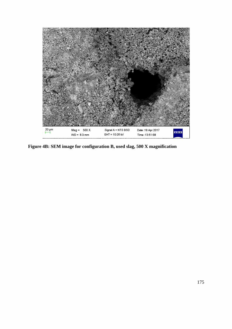
175

Figure 4B: SEM image for configuration B, used slag, 500 X magnification

176

Figure 5B: SEM image for configuration C, used slag from second column, 500 X

magnifications

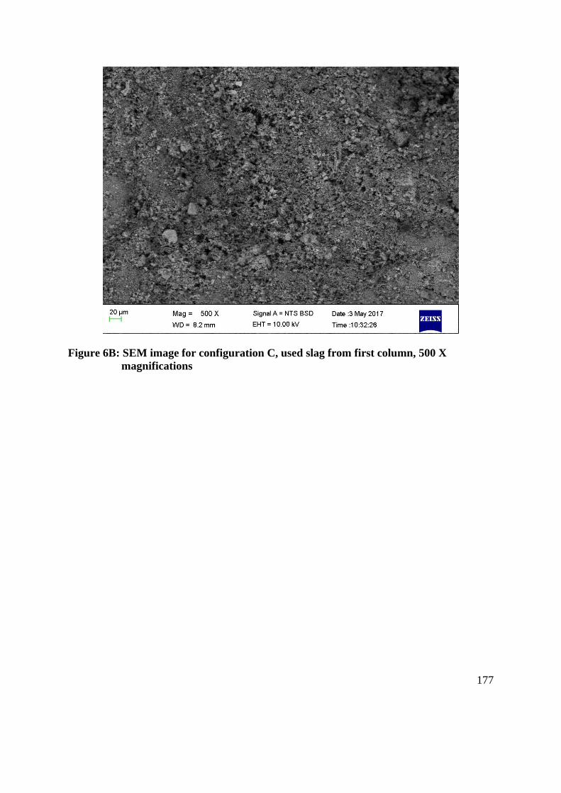
177

Figure 6B: SEM image for configuration C, used slag from first column, 500 X

magnifications

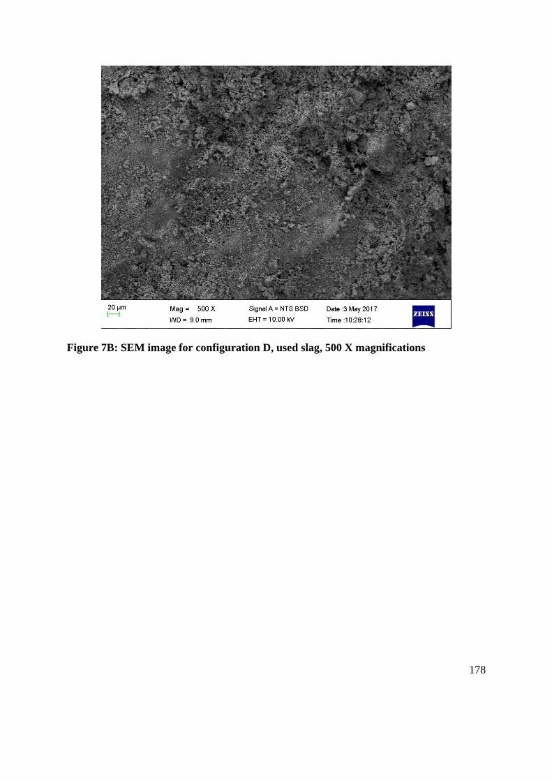
178

Figure 7B: SEM image for configuration D, used slag, 500 X magnifications

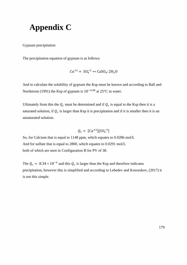
179

Appendix C

Gypsum precipitation

The precipitation equation of gypsum is as follows:

𝐶𝑎+2 + 𝑆𝑂4−2 ↔ CaSO4: 2H2O

And to calculate the solubility of gypsum the Ksp must be known and according to Ball and

Nordstrom (1991) the Ksp of gypsum is 10−4.58 at 25°C in water.

Ultimately from this the 𝑄𝑐 must be determined and if 𝑄𝑐 is equal to the Ksp then it is a

saturated solution, if 𝑄𝑐 is larger than Ksp it is precipitation and if it is smaller then it is an

unsaturated solution.

𝑄𝑐 = [𝐶𝑎+2][𝑆𝑂4−2]

So, for Calcium that is equal to 1148 ppm, which equates to 0.0286 mol/L

And for sulfate that is equal to 2800, which equates to 0.0291 mol/L

both of which are seen in Configuration B for PV of 38.

The 𝑄𝑐 = 8.34 ∗ 10−4 and this 𝑄𝑐 is larger than the Ksp and therefore indicates

precipitation, however this is simplified and according to Lebedev and Kosorukov, (2017) it

is not this simple.

Documents

Remediation of Acid Mine Drainage utilizing sugar cane