Embed Size (px)
Citation preview

Electronic copy available at: http://ssrn.com/abstract=1335855
Religious Beliefs, Gambling Attitudes,and Financial Market OutcomesI
Alok Kumara,b,∗, Jeremy K. Pagea, Oliver G. Spaltc
aUniversity of Texas at Austin, 1 University Station B6600, Austin, TX 78705bUniversity of Miami, 514 Jenkins Building, Coral Gables, FL 33124
cTilburg University, 5000 LE, Tilburg, The Netherlands
Abstract
We use religious background as a proxy for gambling propensity and investigate whether geographic
variation in religion-induced gambling norms affects aggregate market outcomes. We examine four
economic settings in which the recent literature has suggested a role for gambling and specula-
tion. Our key conjecture is that gambling propensity would be stronger in regions with higher
concentration of Catholics relative to Protestants. Consistent with our conjecture, we find that
religion-induced gambling preferences influence the portfolio decisions of institutional investors.
Investors located in regions with a higher Catholic-Protestant ratio (CPRATIO) exhibit a stronger
propensity to hold stocks with lottery features. In a corporate setting, we show that broad-based
employee stock option plans, which would appeal more to employees with stronger gambling prefer-
ences, are more popular in higher CPRATIO regions. Examining the aggregate impact of gambling
on stock returns, we find that the initial day return following an initial public offering is higher for
firms located in high CPRATIO regions where local speculative demand is expected to be stronger.
In a broader market setting, we find that the magnitude of the negative lottery-stock premium is
larger in high CPRATIO regions. Collectively, our results indicate that religious beliefs, through
their influence on gambling attitudes, impact investors’ portfolio choices, corporate decisions, and
IWe would like to thank an anonymous referee, Nick Barberis, Sudheer Chava, James Choi, Joost Driessen,Xavier Gabaix, Hamed Ghoddusi, Will Goetzmann, John Griffin, Gilles Hilary, Kai Wai Hui, Shimon Kogan, GeorgeKorniotis, Alexandra Niessen, Amiyatosh Purnanandam, Mohammad Rahaman (NFA discussant), Enrichetta Ravina(NBER discussant), Clemens Sialm, Laura Starks, Luke Taylor (EFA discussant), and seminar participants at the2009 NFA Meetings (Niagara-on-the-Lake), 2009 EFA Meetings (Bergen), 2009 Yale Behavioral Finance Conference,2010 NBER Behavioral Finance Meeting, and UT-Austin for helpful discussions and valuable comments. We alsothank Garrick Blalock, Will Goetzmann, and Jacqueline Yen for the lottery sales data. We are responsible for allremaining errors and omissions.
∗Corresponding author.Email address: [email protected] (Alok Kumar)
Preprint submitted to Journal of Financial Economics April 1, 2011

Electronic copy available at: http://ssrn.com/abstract=1335855
stock returns.
Keywords: gambling, religion, institutional investors, employee stock option plans, IPOs
JEL: G11, G12, Z12
1. Introduction
Gambling and speculation play an important role in financial markets. These and related activ-
ities are often associated with high levels of trading volume, high return volatility, and low average
returns (e.g., Scheinkman and Xiong, 2003; Hong et al., 2006; Grinblatt and Keloharju, 2009; Dorn
and Sengmueller, 2009). As gambling attains wider acceptability in society and a “lottery culture”
emerges (e.g., Shiller, 2000), the influence of gambling behavior in financial markets is likely to
increase and could have economically significant effects on corporate decisions and stock returns.
Specifically, in market settings that superficially resemble actual gambling environments and in
which skewness is a salient feature, people’s gambling attitudes may influence aggregate market
outcomes.
For example, if the positively skewed returns of initial public offering (IPO) stocks lead investors
to perceive IPOs as lotteries, their preference for lottery-like payoffs and trading behavior could
generate initial overpricing (e.g., Barberis and Huang, 2008). More generally, if investors exhibit
a preference for stocks with lottery features, all else equal, stocks with lottery-type characteristics
would earn lower average returns.1 Similarly, the popularity of broad-based employee stock option
(ESO) plans has been difficult to explain within the traditional economic framework (e.g., Oyer and
Schaefer, 2004; Bergman and Jenter, 2007; Kedia and Rajgopal, 2009). One potential explanation
for this puzzle is that option grants to non-executives reflect the gambling preferences of rank and
file employees (e.g., Spalt, 2009). Individuals with strong gambling preferences may find firms that
offer option-based compensation plans attractive if they view stock options as “lottery tickets”.2
Some managers may even attempt to cater to those preferences.
1Motivated by the salient features of state lotteries (low price, low negative expected return, and risky as wellas skewed payoff) and the theoretical framework of Barberis and Huang (2008), Kumar (2009) defines stocks thathave low prices, high idiosyncratic volatility, and high idiosyncratic skewness as lottery-type stocks. In contrast,non-lottery-type stocks have high prices, low idiosyncratic volatility, and low idiosyncratic skewness. See Section 2for an additional discussion.
2The conjecture that certain employees are likely to perceive stock options as gambles is supported by the evidencethat employees frequently value options higher than the actuarially fair value (e.g., Hodge et al., 2010; Hallock andOlson, 2006; Devers et al., 2007) and the finding that riskier firms grant more employee stock options (Spalt, 2009).
2

Electronic copy available at: http://ssrn.com/abstract=1335855
The important role of gambling in various market settings has been recognized in the recent
asset pricing and corporate finance literatures. However, it has been difficult to attribute aggregate
market outcomes directly to people’s gambling preferences because individual-level gambling and
speculative activities cannot be directly observed. In this paper, we use people’s religious beliefs
as a proxy for their gambling propensity and examine whether geographical variation in religious
composition, particularly the variation in the ratio of Catholics to Protestants across U.S. counties,
allows us to identify market-wide effects of gambling behavior.
Our choice of religious composition as a proxy for gambling propensity is motivated by the
observation that gambling attitudes are strongly determined by one’s religious background. In
particular, the Protestant and Catholic churches have very distinct views on gambling.3 A strong
moral opposition to gambling and lotteries has been an integral part of the Protestant movement
since its inception, and many Protestants perceive gambling as a sinful activity (e.g., Starkey, 1964;
Ozment, 1991; Ellison and Nybroten, 1999). Although individual Protestant churches vary in the
intensity with which they oppose gambling, the opposition to gambling is quite general. The largest
Protestant group, the Southern Baptists, is particularly strident in their censure of gambling.
In contrast, the Roman Catholic church maintains a tolerant attitude towards moderate levels
of gambling and is less disapproving of gambling activities. It has even used gambling in the form
of bingo and charitable gaming events as an important source of fund-raising (e.g., Diaz, 2000;
Hoffman, 2000). Among other prominent religious denominations in the U.S., people of Jewish
faith behave similar to Catholics and accept gambling activities more readily, while the gambling
attitudes of Latter-Day Saints (Mormons) are aligned more closely with those of Protestants.
The impact of these diverse viewpoints on gambling is evident in state lottery adoption policies
3The gambling views typical of many Protestant churches are expressed in the United Methodist Church’s 2004Book of Resolutions: “Gambling is a menace to society, deadly to the best interests of moral, social, economic, andspiritual life, and destructive of good government. As an act of faith and concern, Christians should abstain fromgambling and should strive to minister to those victimized by the practice.” The position of the Catholic Church ongambling is summarized in the New Catholic Encyclopedia: “A person is entitled to dispose of his own property as hewills. . . so long as in doing so he does not render himself incapable of fulfilling duties incumbent upon him by reasonof justice or charity. Gambling, therefore, though a luxury, is not considered sinful except when the indulgence init is inconsistent with duty.” Further, The Catechism of the Catholic Church (2413) states: “Games of chance (cardgames, etc.) or wagers are not in themselves contrary to justice. They become morally unacceptable when theydeprive someone of what is necessary to provide for his needs and those of others. The passion for gambling risksbecoming an enslavement. Unfair wagers and cheating at games constitute grave matter, unless the damage inflictedis so slight that the one who suffers it cannot reasonably consider it significant.” Thompson (2001, pages 317-324)provides a summary of the gambling views of major religious denominations in the U.S.
3

and levels of lottery expenditures. Prior empirical research has shown that the popularity of
state lotteries in a region is affected by the dominant local religion (e.g., Berry and Berry, 1990;
Martin and Yandle, 1990; Ellison and Nybroten, 1999). A few recent studies also demonstrate that
religion-induced gambling attitudes carry over into financial decisions (e.g., Kumar, 2009; Doran
et al., 2011). We confirm these findings using our county-level measures of religious composition.
In particular, we show that states with higher concentration of Catholics relative to Protestants
(i.e., higher Catholic-Protestant ratio (CPRATIO)) are more likely to legalize state lotteries and
adopt them earlier. Further, at both state and county levels, we find that per capita lottery sales
are higher in regions with high CPRATIO. We also show that individual investors located in high
CPRATIO regions assign larger portfolio weights to lottery-type stocks (see Figure 1) and confirm
that religion-induced gambling attitudes carry over into financial decisions.
Motivated by these empirical findings, we conjecture that religion-induced heterogeneity in
gambling preferences and behavior could affect economic decisions in other settings. In particular,
the predominant local religion could influence local cultural values and norms and consequently
affect the financial and economic decisions of individuals located in that region, even if they do
not personally adhere to the dominant local faith.4 Further, these financial and economic decisions
could aggregate and generate market-wide forces that can potentially influence aggregate financial
market outcomes.
We consider four specific economic settings in which the existing literature has suggested the
possible role of gambling and examine the link between religious beliefs, gambling attitudes, and
aggregate market outcomes. First, we examine the extent to which geographical heterogeneity in
religious beliefs influences investors’ portfolio choices. We find that the portfolio characteristics of
institutional investors are influenced by the religious characteristics of the neighborhoods in which
they are located. Although institutions on average tend to avoid lottery-type stocks (e.g., Kumar,
2009), institutions located in high CPRATIO regions assign larger weights to stocks with lottery
4We do not use the local religion measures to identify the religious background of the individual making a decision.While individual religious background is important in shaping gambling attitudes, we assume that the dominantlocal religion shapes the local culture, which in turn has the potential to systematically affect the decisions of localindividuals in different settings, including economic decisions. For example, the decisions of an individual located inUtah might be influenced by the local Mormon culture even if the person is not a Mormon. Similarly, a Catholic inProtestant-dominated Tennessee might at least partially be influenced by local Protestant cultural norms.
4

features and simultaneously under-weight non-lottery-type stocks. The impact of local religious
norms on portfolio decisions is significant only among smaller and moderate-sized institutions.
Among larger institutions with more standardized investment practices (e.g., Baker et al., 2011),
local religious environment is not a significant determinant of institutional portfolio decisions.
Further, the religion-induced differences in stock holdings are stronger among “aggressive” in-
stitutions and those institutions that trade more actively or hold concentrated portfolios containing
few stocks. Over time, preference for lottery-type stocks is amplified during the end of the year
when the temptation to engage in risk-seeking and gambling-type activities is likely to be stronger
due to performance-based incentives (Brown et al., 1996). We conduct several tests to ensure that
these results are not induced by geographical clustering of institutions in a few large counties and
financial centers or due to repeated observations.
Second, we investigate a corporate finance puzzle: Why do firms grant options to non-executive
rank and file employees? We show that broad-based employee stock option plans, which would
appeal more to employees with strong gambling preferences, are more popular in high CPRATIO
regions where individuals are likely to exhibit a stronger propensity to gamble. Further, consistent
with our gambling interpretation, we find that the sensitivity of the level of non-executive option
grants to local religious composition is greater among high volatility firms, which would be more
attractive to individuals with strong gambling preferences due to their higher skewness. These re-
sults indicate that the puzzle of broad-based employee stock option plans could at least be partially
resolved within a theoretical framework that recognizes the potential link between compensation
and gambling.
Third, we focus on the IPO markets and test one of the key empirical predictions of the Barberis
and Huang (2008) model. They conjecture that excess speculative demand of skewness-loving
investors can generate overpricing in securities such as IPOs that have positively skewed returns.
Consistent with this conjecture, we find that the initial day return following an initial public offering
is higher for IPO firms located in high CPRATIO regions where the propensity to gamble is likely
to be higher. To strengthen the link between first-day IPO return and gambling propensity of
local investors, we show that the relation between initial day returns and CPRATIO is stronger
in regions with higher stock market participation rates (as proxied by higher income and higher
education levels) and stronger local bias. In these areas, local investors are more likely to trade
5

local IPOs and, thus, more likely to play a marginal price-setting role. Collectively, our IPO results
indicate that the puzzling phenomenon of IPO underpricing is at least partially influenced by the
gambling behavior of local investors.
In the last part of the paper, we study the effect of gambling on stock returns in a broader
market setting. Specifically, we investigate the pricing of stocks with lottery-type characteristics.
This exercise is also motivated by the theoretical predictions in Barberis and Huang (2008), who
conjecture that securities with lottery features are expected to earn lower average returns because
investors are willing to accept lower average returns for a tiny probability of a large potential gain.
Consistent with their conjecture, we find that lottery-type stocks earn lower average returns. In
addition, consistent with our gambling hypothesis, we find that the magnitude of the negative
lottery-stock premium is stronger in regions with high CPRATIO.
Our empirical findings are robust to a large number of variations to the baseline specifica-
tions. In particular, when we use the Rajan and Zingales (1998) method to account for unobserved
heterogeneity at the state- and county-levels, we obtain results that are qualitatively similar to
our baseline results. Overall, our empirical results indicate that religion-induced gambling norms
influence gambling preferences, individual-level economic decisions, and aggregate market-level out-
comes. Both corporate policies and asset prices are influenced by religion-induced local gambling
propensity.
These results complement recent evidence in Hilary and Hui (2009) and show that religion
influences financial market outcomes not only through the risk aversion channel but also through
its effect on the skewness and gambling preferences of individuals.5 Further, while previous studies
indicate that religion could influence economic growth (Barro and McCleary, 2003) and the level of
investor protection in a country (Stulz and Williamson, 2003), our results highlight the importance
of religious composition at a more disaggregate individual and firm level. In broader terms, our
empirical evidence contributes to the emerging literature in economics that examines the interplay
between culture and economic outcomes (e.g., Guiso et al., 2003, 2006). Because religion is a key
5Hilary and Hui (2009) examine the effect of corporate culture on economic decisions. They show that corporatepolicies of firms located in more religious areas are more conservative and reflect higher levels of risk aversion.Specifically, when the county-level religiosity is high, firms have lower risk exposures, require higher internal rates ofreturn before investing in risky projects, and experience lower long-term growth.
6

cultural attribute, our results indicate that through its impact on people’s gambling attitudes,
cultural shifts can influence aggregate financial market outcomes.
The rest of the paper is organized as follows. In the next section, we summarize our key testable
hypotheses. We describe our main data sources in Section 3 and motivate the choice of our gambling
proxy in Section 4. We present our main empirical results in Section 5 and conclude in Section 6
with a brief summary.
2. Related Literature and Testable Hypotheses
We develop our gambling-motivated hypotheses in four distinct economic settings where the
existing literature has emphasized the potential role of gambling and speculation in determining
the aggregate market outcome. We assume that the religious composition of a region would reflect
the gambling attitudes of local individuals. In particular, given the differences in the religious
teachings and the related empirical evidence, we conjecture that Catholics (Protestants) are likely
to exhibit a higher (lower) propensity to gamble.
In the first economic setting, we examine whether local gambling attitudes influence the port-
folio decisions of local institutional investors. Specifically, we investigate whether the institutional
preference for stocks with lottery features varies with the religious characteristics of institutional
location. Our choice is motivated by the evidence in Kumar (2009), who shows that the so-
cioeconomic characteristics of retail investors, including the religious characteristics of their local
neighborhood, influence their investment in lottery-type stocks. We extend this insight to institu-
tional investors and argue that religion-induced local cultural norms would influence institutional
portfolio decisions.
Lottery-type stocks represent low cost investments with very high potential reward to cost ratio.
Just as state lotteries have very low prices relative to the highest potential payoff, low negative
expected returns, and risky as well as positively skewed payoffs, Kumar (2009) identifies stocks
that have low prices, high idiosyncratic volatility, and high idiosyncratic skewness as lottery-type
stocks. This definition is also motivated by the theoretical model of Barberis and Huang (2008),
where investors overweight low probability events and exhibit a preference for stocks with positive
7

skewness.6 In contrast, stocks have high prices, low idiosyncratic volatility, and low idiosyncratic
skewness are classified into the non-lottery-type category.7
Although a typical institution is likely to avoid risky, lottery-type stocks due to prudent man
rules and other institutional constraints (e.g., Badrinath et al., 1989; Del Guercio, 1996), some
institutions might gravitate toward these stocks because they provide “cheap bets” and offer good
opportunities for exploiting information asymmetry. In particular, the institutional attraction for
smaller, lottery-type stocks might increase over time as competition in other market segments
increases (e.g., Bennett et al., 2003).
Within the group of institutions, there are potentially important differences between very large
institutions, such as Fidelity, and other institutions. Large institutions are likely to have a more
diverse customer base, offices across the county, more standardized investment processes, and are
potentially more influenced by common benchmarking practices (e.g., Baker et al., 2011). In con-
trast, smaller institutions may have greater latitude to invest aggressively and could hold larger
positions in lottery-type stocks. Further, the customer base of smaller institutions may be local
and the gambling preferences of that local clientele could influence institutional portfolio decisions.
Given these differences across institutions, we expect that religious beliefs would influence the
investment decisions of only small and moderate-sized institutions. Overall, we posit that:
H1: Institutional gambling preference: Small and medium-sized institutions located
in regions with high concentration of Catholics would exhibit a stronger preference
for lottery-type stocks than comparable institutions located in Protestant-dominated
regions.
To gather additional support for the institutional gambling hypothesis, we examine whether
the gambling propensity and its effect on portfolio decisions vary with institutional type and over
time. This conjecture is motivated by the observation that certain types of institutions such as
banks and insurance companies are known to hold conservative portfolios and are therefore less
likely to engage in speculative activities. Further, performance based incentives could exacerbate
6In a similar spirit, Markowitz (1952) conjectures in one of the early studies that some investors might prefer to“take large chances of a small loss for a small chance of a large gain.”
7See Section III in Kumar (2009) for further motivation behind this definition of lottery-type stocks and also fora summary of the properties of lottery-type stocks.
8

the gambling temptations of institutions who are predisposed to gamble. More specifically, we
conjecture that:
H1b: Institutional characteristics and gambling preference: The religion-lottery weight
relation would be stronger among institutions that hold concentrated portfolios and
weaker among conservative institutions. Further, the religion-lottery weight relation
would be stronger around year-end when performance incentives would induce institu-
tions located in regions with large Catholic concentration to gamble more aggressively.
Next, we investigate a corporate finance puzzle and examine whether the widespread popularity
of broad-based employee stock option plans reflects the gambling preferences of non-executive
employees. Employees frequently value options higher than their actuarially fair values (e.g., Hodge
et al., 2010; Hallock and Olson, 2006; Devers et al., 2007) and riskier firms grant more employee
stock options (e.g., Spalt, 2009). This evidence is consistent with the hypothesis that employees
perceive stock options as long shot gambles. If firms are aware that option-based compensation
plans are more attractive to employees with stronger gambling preferences, they might even cater
to those preferences to reduce the overall compensation costs. Motivated by these possibilities, we
conjecture that:
H2a: Employee gambling preference: Broad-based employee stock option plans would
be more popular among firms that are located in regions with a higher concentration of
Catholics relative to Protestants.
To strengthen the link between gambling preferences and popularity of non-executive ESO plans,
we examine whether the ESO-religion relation is stronger within the subset of higher volatility
firms that are likely to be more attractive to employees with gambling preferences because of their
higher skewness. Specifically, we test the following hypothesis:
H2b: Firm volatility and employee gambling preference: The religion-option value rela-
tion would be stronger among high volatility firms because Catholics (Protestants) are
likely to find them more (less) attractive.
In the next two economic settings, we use our gambling proxy to examine the potential asset
pricing implications of gambling. We first study the IPO markets where gambling and speculative
9

activities are likely to be more prevalent. Barberis and Huang (2008) show that in an economy with
cumulative prospect theory investors, low probability events are overweighted and, consequently,
securities such as IPOs that have positively skewed returns can be overpriced in the short-run.
If the propensity to over-weight the tiny probabilities of large initial gains and the preference for
skewed payoffs vary with religious beliefs, the degree of initial overpricing would vary with the
religious composition of the county in which an IPO firm is located. More formally, our third main
hypothesis is:
H3a: Gambling-induced initial day IPO return: The initial day return would be higher
for IPOs located in regions with higher concentration of Catholics relative to Protes-
tants.
This hypothesis is based on the implicit assumption that the preferences of local investors are
reflected in first-day IPO returns. A necessary condition for this assumption to hold is that local
investors participate in the stock market and exhibit a preference for local stocks. Therefore, the
religion-IPO return relation should be stronger in regions with higher market participation rates
and stronger local bias. To test this possibility, we conjecture that:
H3b: Local bias and first-day IPO return: The religion-first-day return relation would
be stronger for IPO firms that are located in regions with higher stock market partic-
ipation rates (as proxied by higher income and higher education levels) and stronger
local bias.
Last, we examine the link between gambling preference and stock returns in a broader market
setting. Motivated again by the theoretical predictions in Barberis and Huang (2008), we investigate
the pricing of stocks with lottery-type characteristics. According to theory, these stocks with high
idiosyncratic volatility, high idiosyncratic skewness, and low prices are expected to earn low average
returns. We examine whether the religious characteristics of the county in which lottery-type firms
are located affect the magnitude of the negative lottery stock premium. Specifically, given the
known differences in the gambling attitudes of Protestants and Catholics, we conjecture that:
H4: Lottery-stock premium: The magnitude of the negative lottery-stock premium
would be larger for the subset of firms located in regions with higher concentration of
Catholics relative to Protestants.
10

To test these four sets of hypotheses, we use data from several different sources. We briefly
describe those data sets in the following section.
3. Data and Summary Statistics
3.1. County-Level Religious and Demographic Characteristics
Our first main data set captures the county-level geographical variation in religious composition
across the U.S. We collect data on religious adherence using the “Churches and Church Member-
ship” files from the American Religion Data Archive (ARDA). The data set compiled by Glenmary
Research Center contains county-level statistics for 133 Judeo-Christian church bodies, including
information on the number of churches and the number of adherents of each church. During our
1980 to 2005 sample period, the county-level religion data are available only for years 1980, 1990,
and 2000. Following the approach in the recent literature (e.g., Alesina and La Ferrara, 2000; Hilary
and Hui, 2009), we linearly interpolate the religion data to obtain the values in the intermediate
years.
We consider three main religion variables: (i) religiosity of the county defined as the total number
of religious adherents in the county as a proportion of the total population in the county (REL);
(ii) the proportion of Catholics in a county (CATH); and (iii) the proportion of Protestants in a
county (PROT). Using these religion variables, we define the Catholic-Protestant ratio (CPRATIO)
to capture the relative proportions of Catholics and Protestants in a county. Our main focus is on
the CPRATIO variable and we consider other related religion variables for robustness.
Figure 1 shows the geographical variation in the county-level religiosity and religious composi-
tion across the U.S. counties. It is evident that the religiosity levels are lower on the two coasts
and significantly higher in the Central region. For example, the state of Utah has one of the high-
est levels of religiosity. Examining the geographical variation in the proportion of Catholics and
Protestants, we find that Catholics are concentrated more on the Eastern and Western coasts, while
the Protestant concentration is greater in the Mid-Western and Southern regions.
We obtain additional county-level demographic characteristics from the U.S. Census Bureau.
Specifically, we consider the total population of the county, the county level of education (the
proportion of county population above age 25 that has completed a bachelor’s degree or higher),
11

male-female ratio in the county, the proportion of households in the county with a married couple,
minority population (the proportion of county population that is non-white), per capita income of
county residents, the median age of the county, and the proportion of the county residents who
live in urban areas.8 Similar to Hilary and Hui (2009), we employ these county characteristics as
control variables in our empirical analysis.
Table 1, Panel A reports summary statistics for the county-level religion and demographics data
for all US counties with complete data. Panel B presents the same statistics for all counties based
on the institutional investors sample.9 We have religion and demographics data for 3,092 counties
and institutions are located in 415 of those counties.10 The typical (median) firm is located in a
county in which 17.44% of the population is Catholic and 24.95% adheres to the Protestant faith.
This is in contrast to the typical county in the United States, in which 8.62% of the population
is Catholic and 40.37% of the population is Protestant. These statistics indicate that firms in the
United States tend to cluster in areas with higher concentration of Catholics. Nevertheless, there is
substantial independent variation in both religion variables. For example, the 25th percentile value
of CPRATIO is 0.25 and its 75th percentile value is significantly higher (= 1.63).
The typical firm in our sample is also located in relatively high-income ($24,613 in our sample
versus $16,772 in the typical county) and well-educated areas (22.97% of the population above the
age of 25 in our sample has college degrees versus 12.65% in the median county). Further, those
firms are located in urban areas (82.99% of the county population in our sample lives in urban
regions versus 36.60% in the typical county) and regions with greater concentration of minorities
(14.57% in our sample versus 6.97% in the median county).
3.2. Institutional Ownership and Portfolio Weights in Lottery Stocks
Our second main data set is the quarterly common stock holdings of 13(f) institutions compiled
by Thomson Reuters. The sample period is from 1980 to 2005. We identify the institutional
location (zip code) using the Nelson’s Directory of Investment Managers and by searching the SEC
documents and web sites of institutional managers.
8Although data on the average household income are available, we do not include income in our empirical analysisbecause it is highly correlated with the education proxy (correlation = 0.82).
9The religion statistics based on our employee stock option or IPO samples are qualitatively similar. For brevity,we do not report those estimates.
10In comparison, firms in the CRSP sample are located in 1,088 counties during the same time period.
12

Every quarter, for each institutional portfolio, we compute the portfolio weight allocated to
lottery-type stocks. Motivated by Kumar (2009), we define lottery-type stocks using idiosyncratic
volatility and idiosyncratic skewness measures. A stock is considered “lottery-type” if it has above-
median volatility and above-median skewness. Both the volatility and skewness measures are
obtained using past six months of daily returns data. We do not use stock price as one of the
lottery stock attributes because prudent man rules and other constraints prevent institutions from
holding very low priced stocks.11 For robustness, motivated by the conjecture in Barberis and
Huang (2008), we also assume that recent IPOs could be perceived as stocks with lottery features.
Since our institutional gambling hypothesis applies mainly to small and moderate-sized insti-
tutions, we exclude very large institutions from our main sample. In each quarter we identify
institutions with portfolio size above the average portfolio size across all institutions in the quarter
and classify them as “very large institutions”. Using this classification method, we find that the
number of very large institutions increases from 110 in the first quarter of 1980 to 239 in the last
quarter of 2005. The portfolio size cutoff varies from $711 million in the first quarter 1980 to $5.79
billion in the last quarter of 2005. During our sample period, an average of 18.48% institutions
are identified as very large and the average portfolio size cutoff used for this classification is $2.53
billion. The average portfolio size of a very large institution is $16.47 billion, while the average size
of institutions in our baseline sample is only $544 million. As shown in Panel C of Table 2, there
are 19,601 institution-quarter observations that are associated with very large institutions, which
leaves 101,377 observations in the baseline sample.
Table 2 also shows the ten largest counties identified using the portfolio holdings of institutions
located within the county. For each of the ten counties, we report the proportional holdings
of county-level institutions in the aggregate institutional portfolio, the fraction of institutional
observations that are from the county, and the average county-level CPRATIO. A large fraction
of the institutions in our sample are located in large financial centers such as New York, Boston,
Chicago, Los Angeles, and San Francisco. For comparison, in Panel D of Table 2, we report the
county-level statistics for the ten largest counties based on the market capitalization of publicly-
11In our robustness section, we show that these results are qualitatively similar when we use stock price and definea stock as lottery-type if it has below-median price, above-median volatility, and above-median skewness.
13

traded firms located within the county. About 24% of observations in the sample of publicly-traded
firms are from the largest ten counties, while about 43% of institutional observations are from the
largest ten counties. Thus, both firms and institutions exhibit geographical clustering, where the
degree of clustering is greater among institutions.
Table 1, Panel C reports county-level summary statistics for the institutional investor sample.
The typical (median) institution assigns a portfolio weight of 5.09% to lottery-type stocks. However,
the distribution of lottery stock portfolio weights is skewed as the mean is considerably higher
(= 9.49%). This evidence suggests that some institutions may “specialize” and commit substantial
portions of their portfolios to stocks with lottery features. In contrast, the median institution
holds nearly 44.50% of its portfolio in non-lottery stocks that have relatively low volatility and low
skewness. The mean institutional portfolio weight in recent IPOs (firms that went public in the
previous quarter) is 0.28%. When we consider the set of non-local IPOs (firms located more than
250 miles away from the institutional location), the mean weight is only 0.17%.
The typical institutional portfolio’s size is $279 million. Portfolio concentration, measured as
the Herfindahl index of institutional portfolio weights, has a median estimate of 0.027 and a mean
of 0.068. In the typical county we have one observation per quarter, but the mean is considerably
higher (= 3.28).
3.3. Stock Option Grants to Non-Executives
Our third main data set contains option grants to non-executive rank and file employees. We
follow the recent ESO literature (e.g., Desai, 2003; Bergman and Jenter, 2007) and use ExecuComp
to obtain estimates of options granted to non-executives. Firms are not required to disclose details
about their stock option programs to non-executive employees but ExecuComp reports the number
of options granted to each of the top five executives during a year. In addition, for each top
executive, ExecuComp variable pcttotopt indicates the share of their option grant as a percentage
of the total number of stock options granted by the firm during a fiscal year. Using the information
on the individual option grants to top executives and these percentages, we are able to estimate
the total number of options granted by the firm.
To obtain estimates of option grants to non-executive rank and file employees, we subtract the
option grants to executives from the total number of options granted. We obtain the option grants
14

to top executives using the ExecuComp data and use the method of Oyer and Schaefer (2004) to
estimate the number options awarded to high-level executives not listed in ExecuComp, but for
whom option grants may reasonably have incentive effects.12 The number of employees reported
in ExecuComp is used to calculate per-employee values of option grants. We obtain the number of
options granted per non-executive employee by dividing the total option grants to non-executives
by the total number of firm employees less the estimated number of high-level executives.
We compute the Black-Scholes values of non-executive option grants using the average of the
grant date stock price reported in ExecuComp for all grants in a given firm-year. Option maturity
and risk-free rate of interest are uniformly set to 7 years and 5%, respectively. Additional details
about the construction of the non-executive option grant measure are available in Spalt (2009).
The initial ESO sample consists of all companies in the ExecuComp database for the 1992 to
2005 period. We exclude firms for which our procedure for identifying incentive-based option grants
is likely to be inaccurate. Specifically, we drop firms with less than 40 employees or less than two
reported executives. We further drop all firms in the financial sector (SIC codes 6000 to 6999) and
all company-years in which the value of one of the independent variables in our baseline regression
specification is missing. The resulting data set has 14,557 firm-year observations for 2,172 unique
firms.
We use several firm characteristics as control variables in our empirical analysis. Specifically, we
control for firm size using the log of sales. We account for investment opportunities using Tobin’s
Q (book assets minus book equity plus market value of equity, scaled by total assets) and research
and development expenses (the three year average of research and development expense scaled by
total assets). All balance sheet data for the ESO sample are taken from Compustat and stock
prices and returns data are obtained from the CRSP-Compustat merged database.
Table 1, Panel D reports the summary statistics for the ESO sample. The median firm in the
sample has 5,032 employees, a market capitalization of $1.08 billion and sales of $1.01 billion. The
median Tobin’s Q and R&D expenses are 1.61 and 0.18%, respectively. A broad-based employee
stock option plan exists in 58.38% of firm-years. In a median firm-year, options are granted on 1.88%
12We assume that the number of high-level executives in a firm can be approximated by the square root of thetotal number of employees. Further, like Oyer and Schaefer (2004), we assume that a high-level executive (excludingthe top five executives) on average receives 10% of the average number of options granted to a top five executive.
15

of total shares outstanding. The Black-Scholes value of option grants to non-executive employees is
low, with a median value of only $166 per employee. However, this distribution is skewed and the
mean value of $4,103 per employee is significantly higher. In addition, these option grant estimates
are biased downward because in most firms not all employees are offered options. In the typical
county in our sample we have 1.40 firms per year, while the mean is higher (= 3.51).
3.4. IPO Data
Our fourth main data set contains information about all initial offerings of common stocks
during the 1980 to 2005 period. We obtain several attributes of IPOs from the Securities Data
Corporation (SDC), including the offer date, offer price, zip code, initial filing price range, lead
underwriters, and gross spread charged by the underwriters. The founding dates for the issuing
firms and Carter and Manaster (1990) rankings for the lead underwriters are from Jay Ritter’s web
site.13 We obtain closing prices for the first day of trading as well as first-day trading volume from
CRSP.
To be included in the sample, the offering must have a CRSP share code of 10 or 11. Further,
the first day of trading recorded by CRSP must be within three days of the SDC offer date. In most
of our analysis, we require the initial offer price to be above $5, but we examine the sensitivity of
our results when this constraint is relaxed. Our final IPO sample consists of 6,652 firms.
Table 1, Panel E reports summary statistics for the IPO sample. The mean first-day return
is 16.55% and there is substantial variation in this measure. It ranges from 0.63% at the 25th
percentile to 21.43% at the 75th percentile. The mean turnover on the first day of trading is high
(= 20.53%) as compared to the daily turnover for the average CRSP firm (≈ 0.50%). The typical
IPO raises $33.05 million and the average firms goes public 8 years after being founded. 32.41%
of the IPO firms in the sample are identified as technology firms, where following Loughran and
Ritter (2004) the technology firm dummy is set to one for firms with an SIC code of 3570 to 3579,
3661, 3674, 5045, 5961, or 7370 to 7379. In the typical county among the set of 610 counties in the
IPO sample, there is one new public offering per year.
13The data are available at http://bear.cba.ufl.edu/ritter/ipodata.htm.
16

3.5. Other Data Sources
We gather data from several additional sources to construct other variables used in our empirical
analysis. Specifically, we use data from a major U.S. discount brokerage house, which contain all
trades and end-of-month portfolio positions of a sample of individual investors during the 1991
to 1996 time period.14 We obtain state-level measures of stock market participation rates from
the Federal Reserve Board. These participation rates are computed from dividend income data
reported on IRS tax returns. We obtain annual state lottery sales data for each state from the
North American Association of State and Provincial Lotteries. We obtain price, volume, return,
and industry membership data from the Center for Research on Security Prices (CRSP). The firm
headquarter location data are from the CRSP-Compustat merged file. Finally, we obtain monthly
values of the market (RMRF), size (SMB) and value (HML) factors from Kenneth French’s web
site.15
In our robustness checks, we use the Bushee (1998) classification method to categorize the 13(f)
institutions into quasi-indexers and non-quasi-indexers based on their portfolio turnover and con-
centration measures. Specifically, institutions classified as quasi-indexers have diversified portfolio
holdings and low turnover.16
In some of our robustness tests we also use state-level Presidential elections data and state-
level measures of trust and social capital.17 The Social Capital measure is a composite index
of 14 different state-level measures of community participation, including “group membership,
attendance at public meetings on town or school affairs, service as an officer or committee member
for some local organization, attendance at club meetings, volunteer work and community projects,
home entertaining and socializing with friends, social trust, electoral turnout, and the incidence of
nonprofit organizations and civic associations.” (Putnam, 2000, pages 290-291).
The Trust variable is based on a question in the General Social Survey that is conducted
biannually since 1974 by the National Opinion Research Corporation at the University of Chicago.
14See Barber and Odean (2000) for additional details about the brokerage data.15The data library is at http://mba.tuck.dartmouth.edu/pages/faculty/ken.french/data library.html.16See http://accounting.wharton.upenn.edu/faculty/bushee/IIclass.html. The classification data corrects
the known errors in the institution types data beyond 1997.17The election data are obtained from David Leip’s web site (www.uselectionatlas.org), while the trust and
social capital data are from Robert Putnam’s Bowling Alone web site (www.bowlingalone.com).
17

It measures the percentage of survey respondents in the state agreeing with the statement that
“Most people can be trusted.” Both the social capital and trust measures are available for only one
year, but because these measures are relatively stable over time, we assume that they would be a
good proxy for the level of trust and social capital in other years.
4. Choice of a Gambling Proxy
Our testable hypotheses implicitly assume that regional religious composition is an effective
proxy for gambling attitudes. Specifically, motivated by the documented differences in the teachings
of different religious denominations and the evidence from the recent literature, we assume that
people’s gambling propensity would be greater in Catholic-dominated regions than in Protestant-
dominated regions. But before presenting our main empirical results, we provide further empirical
justification for this choice.
4.1. Main Gambling Proxy: County-Level Religious Composition
Gambling activities in financial markets are very difficult to observe directly. Therefore, we
use the exogenous geographical variation in religion as a proxy for gambling. Religion is likely
to be an effective proxy for studying the implications of gambling on financial market outcomes
because religious background is an important determinant of beliefs and preferences that influence
economic and financial decisions. In particular, religious composition of a region is likely to be a
strong predictor of people’s gambling attitudes and it is unlikely to be directly related to aggregate
outcomes in financial markets.
This geography-based identification strategy is similar to Becker (2007) and Becker et al. (2010).
They study the availability of bank loans and firm payout policies using the concentration of seniors
in a geographical region as a proxy for deposit supply and dividend demand, respectively. Like
these two earlier studies, we use the geographical variation in a demographic variable as the main
identification strategy.
Our key gambling proxy is the Catholic-Protestant ratio (CPRATIO) in a given county, but
for robustness, we consider related measures such as the Catholic-Protestant differential (CPDIFF)
18

as an alternative indicator of local gambling attitudes.18 We also use the county-level proportions
of Catholics and Protestants separately as our gambling proxies to ensure that we are capturing
the distinct effects of skewness and gambling preferences rather than individual’s risk preferences.19
Additionally, because the gambling attitudes of Catholics and Jews and of Protestants and Mormons
are similar, we extend the definitions of Catholic and Protestant religious categories to include Jews
and Mormons, respectively.
Other socioeconomic attributes such as age, level of education, income, or gender could also
potentially serve as a gambling proxy because they are known to influence people’s propensity
to gamble (Kumar, 2009). However, compared to religion-based measures, these factors exhibit
relatively less geographical variation (e.g., the male-female ratio). Even in instances in which the
demographic variable exhibits significant variation (e.g., income or education), the direction of
the relation between the demographic variables and gambling is not as clearly established as the
relation between religious beliefs and gambling. For instance, while the propensity to play state
lotteries decreases with income, the propensity to engage in other forms of gambling such as casino
gambling and horse race betting increases with income.
Besides demographic variables, another plausible proxy for gambling behavior in financial mar-
kets is the per capita lottery sales in a region. The lottery sales measure could reliably reflect the
gambling propensity of individuals in a region and it is unlikely to directly affect financial market
outcomes. Unfortunately, lottery sales data for extended time periods are available primarily at the
state-level and this coarseness is likely to considerably diminish the power of our geography-based
identification strategy. It is also difficult to compare lottery sales across regions because state lot-
teries were introduced at different times and per-capita lottery sales of all states at a given point in
time might not reflect an equilibrium outcome. Further, lottery sales data at a more disaggregate
level (county or zip code) are available only for a few states for a short time period.
Given these potential limitations of the lottery sales data, we do not use them in our main
18The C −P differential is the difference between the proportion of Catholics and the proportion of Protestants ina given county.
19Risk aversion increases with religiosity, irrespective of the type of religion. For example, Hilary and Hui (2009)show that the proportions of Catholics and Protestants have similar aggregate effects on corporate policies, althoughProtestants are somewhat more risk averse. In contrast, we expect gambling preferences to be stronger amongCatholics and weaker among Protestants. The differences in the gambling attitudes of Catholics and Protestantspredict opposite effects in our empirical tests and provide greater power to our identification strategy.
19

tests. However, we use these data to demonstrate that local religious composition is likely to be
an appropriate proxy for people’s gambling propensity. Although previous studies have already
shown empirically that the state lottery adoption policies and lottery expenditures are influenced
by the regional religious composition (e.g., Grichting, 1986; Berry and Berry, 1990; Diaz, 2000), we
perform several empirical tests to confirm that gambling propensity, as reflected in the popularity of
state lotteries, is stronger (weaker) in regions with higher concentration of Catholics (Protestants).
The results from these tests are presented in Table 3.
4.2. Local Religious Composition and Popularity of State Lotteries
In the first test, we examine whether the religious composition of U.S. states influences the
state-level lottery adoption policies. We find that states in which lotteries are legal have lower
concentration of Protestants and higher concentration of Catholics. For example, in 1990, U.S.
states with lotteries had 10.37% lower concentration of Protestants and 10.86% higher concentration
of Catholics than states without state lotteries (see Table 3, Panel A).
Next, we present univariate sorting results. Using each of the four religion variables (PROT,
CATH, CPRATIO, and REL), we sort counties into quintiles and compute the equal-weighted
quintile averages of per capita county-level lottery sales. We also measure the average state lottery
age (the number of years since the state lottery adoption year) for counties in the five quintiles. We
find that state lotteries were adopted earlier and that lottery age is higher in Catholic-dominated
regions (see Table 3, Panel B). Further, per capita lottery sales are higher in regions with lower
concentration of Protestants and higher concentration of Catholics. For example, in counties with
high concentration of Catholics (top quintile), per capita lottery sales is $195.51, but in counties
with high concentration of Protestants, per capita lottery sales is only $94.23. Similarly, the state
lottery ages in the highest and lowest CPRATIO quintiles are 24.10 and 3.09 years, respectively.
In the third test, for greater accuracy, we estimate a multi-period probit regression of lottery
existence dummy on various state-level demographics characteristics, including religion. The lottery
existence dummy for a year is set to one if state lotteries are legal in the state during the year. The
sample period is from January 1980 to December 2005. The set of primary independent variables
includes the four religion variables, where we use only one of the religion variables in each regression
specification. Because we use geography-based religion variables, the set of independent variables
20
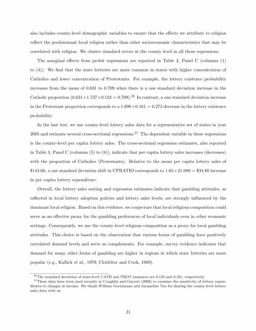
also includes county-level demographic variables to ensure that the effects we attribute to religion
reflect the predominant local religion rather than other socioeconomic characteristics that may be
correlated with religion. We cluster standard errors at the county level in all these regressions.
The marginal effects from probit regressions are reported in Table 3, Panel C (columns (1)
to (4)). We find that the state lotteries are more common in states with higher concentration of
Catholics and lower concentration of Protestants. For example, the lottery existence probability
increases from the mean of 0.631 to 0.709 when there is a one standard deviation increase in the
Catholic proportion (0.631+1.737×0.123 = 0.709).20 In contrast, a one standard deviation increase
in the Protestant proportion corresponds to a 1.698×0.161 = 0.273 decrease in the lottery existence
probability.
In the last test, we use county-level lottery sales data for a representative set of states in year
2005 and estimate several cross-sectional regressions.21 The dependent variable in these regressions
is the county-level per capita lottery sales. The cross-sectional regression estimates, also reported
in Table 3, Panel C (columns (5) to (8)), indicate that per capita lottery sales increases (decreases)
with the proportion of Catholics (Protestants). Relative to the mean per capita lottery sales of
$144.68, a one standard deviation shift in CPRATIO corresponds to 1.65×21.089 = $34.80 increase
in per capita lottery expenditure.
Overall, the lottery sales sorting and regression estimates indicate that gambling attitudes, as
reflected in local lottery adoption policies and lottery sales levels, are strongly influenced by the
dominant local religion. Based on this evidence, we conjecture that local religious composition could
serve as an effective proxy for the gambling preferences of local individuals even in other economic
settings. Consequently, we use the county-level religious composition as a proxy for local gambling
attitudes. This choice is based on the observation that various forms of gambling have positively
correlated demand levels and serve as complements. For example, survey evidence indicates that
demand for many other forms of gambling are higher in regions in which state lotteries are more
popular (e.g., Kallick et al., 1979; Clotfelter and Cook, 1989).
20The standard deviation of state-level CATH and PROT measures are 0.123 and 0.161, respectively.21These data have been used recently in Coughlin and Garrett (2008) to examine the sensitivity of lottery expen-
ditures to changes in income. We thank William Goetzmann and Jacqueline Yen for sharing the county-level lotterysales data with us.
21

It is conceivable that the religious characteristics of a region is correlated with factors such as
the strength of social networks, risk aversion, information sharing propensity, population growth,
growth opportunities, etc. However, it is more difficult to conceive a hypothesis that predicts
opposite relations between one of these measures and local Protestant and Catholic concentration
levels. The opposite influence of Catholic and Protestant beliefs on gambling attitudes is unique
and provides greater power to our identification strategy.22
5. Main Empirical Results
In this section, we use our religion-based gambling proxy to test the four sets of hypotheses
outlined in Section 2. We conduct both univariate and multivariate tests and supplement them
with an extensive set of robustness checks.
5.1. Sorting Results
We begin with a series of univariate tests. Using each of the four religion variables (PROT,
CATH, CPRATIO, and REL), we sort firms into quintiles, where these sorts are performed quarterly
for the institutional dataset and annually for others. We then compute the equal-weighted quintile
averages of institutional portfolio weights in lottery-type and non-lottery-type stocks, the Black-
Scholes value of options granted to non-executive employees, and the first-day IPO return. These
sorting results are presented in Table 4.
In Panel A, corresponding to each of the four religion measures, we report the average insti-
tutional portfolio weights assigned to lottery-type and non-lottery-type stocks in the five religion
quintiles. The evidence indicates that the mean weight in lottery-type stocks decreases as the
Protestant concentration in a county increases. The average portfolio weight allocated to lottery-
type stocks is 11.90% when the Protestant concentration is low (bottom quintile) and it drops to
6.62% in the highest Protestant quintile. In contrast, the weight in lottery-type stocks increases
with Catholic concentration, although the pattern is not monotonic. When Catholic-Protestant
ratio is the sorting variable there is an increasing pattern in the average weight allocated to lottery-
type stocks. The patterns are opposite but weaker when we examine the portfolio weights assigned
22As discussed later, we also use the Rajan and Zingales (1998) method in our main empirical analysis to ensurethat our gambling proxy does not merely reflect the effects of certain omitted variables.
22

to non-lottery-type stocks.
The relation between local religious composition and the lottery-stock preferences of institutions
is similar to the evidence obtained using the stock holdings of retail investors. Figure 2 shows
the univariate sorting results obtained using the retail brokerage data. Like the composition of
institutional portfolios, the mean retail portfolio weight allocated to lottery-type stocks increases
with Catholic concentration and decreases with Protestant concentration. This evidence indicates
that even though the average gambling preferences of retail and institutional investors differ (e.g.,
Kumar, 2009), they exhibit similar sensitivity to local religious characteristics, which are likely to
capture the local gambling “culture”.23 Overall, the institutional sorting results are consistent with
our first main hypothesis (H1a) and indicates that institutional gambling tendencies are sensitive
to local religious composition.
We find a similar pattern when we examine the relation between county-level religious com-
position and non-executive option grants. The Black-Scholes value of option grants per employee
decreases with Protestant concentration and increases with Catholic concentration (see Table 4,
Panel B). For example, the average Black-Scholes value of option grants in the lowest Protestant
quintile is $10,864 and it is only $1,422 in the highest Protestant quintile. Like the institutional
lottery weight results, the sorting results are non-monotonic and weaker when we sort using the
Catholic concentration measure. However, in unreported results, we find a monotonic pattern when
we examine medians. The ESO sorting results are consistent with the hypothesis that individuals
whose religious beliefs discourage gambling are less likely to find option-based compensation attrac-
tive. Alternatively, managers may be less inclined to offer compensation schemes with gambling-like
payoffs to employees in regions where religion-based local social norms condemn gambling. Overall,
the ESO sorting results are consistent with our second main hypothesis (H2a).
In the last set of univariate tests, we focus on the first-day IPO return. These results, also
reported in Panel B, indicate that the mean first-day IPO return decreases monotonically with
Protestant concentration and increases with Catholic concentration. But again, the pattern is
non-monotonic, and exhibits an almost monotonically increasing pattern when Catholic-Protestant
23See Kumar (2009) for additional evidence on the relation between religious composition and the propensity toinvest in lottery-type stocks. In this paper, we partially replicate those results for completeness.
23

ratio is the sorting variable. For example, when the average Protestant concentration increases
from 7.89% to 40.22% across the extreme quintiles, the average first-day IPO return decreases
from 20.05% to 13.85%. Similarly, the average first-day IPO return increases from 13.79% to
18.46% across the extreme Catholic-Protestant ratio quintiles. These univariate sorting results are
consistent with our third main hypothesis (H3a).
The consistency in the patterns in the univariate results across the three distinct economic
settings is striking. In all three instances, the results exhibit a strong monotonic pattern when
the Protestant concentration measure is the sorting variable and an increasing but non-monotonic
pattern when the Catholic concentration measure is the sorting variable. The patterns with the
religiosity measure weakly reflect the sorting results obtained using the Protestant concentration
measure. Taken together, the univariate sorting results are consistent with our key conjecture that
regional religious beliefs influence financial market outcomes through their impact on gambling
attitudes of local individuals.
5.2. Regression Model and the Choice of Independent Variables
To examine whether the significance of the sorting results remain when we account for other
known determinants of aggregate market outcomes, we estimate a series of multivariate regression
models. We use the same empirical framework in the first three settings that we examine. The
dependent variable in these regressions is one of the following three variables: (i) portfolio weight
in lottery-type or non-lottery-type stocks, (ii) Black-Scholes value of non-executive employee stock
option (ESO) grants, and (iii) first-day IPO return. The key independent variable is one of the
four religion variables, where we assume that these geographic measures of religious concentration
would proxy for religion-based differences in gambling attitudes.
We use multiple religion variables to ensure that we are capturing the gambling attitudes of
local individuals rather than other related aspects of their behavior such as risk aversion. In
particular, Hilary and Hui (2009) use the fraction of religious inhabitants per county as a proxy for
risk aversion and show that this variable influences corporate policies of firms with headquarters
in this location. Because religiosity and our gambling proxy (CPRATIO) are positively correlated,
the effects that we document might reflect the level of religiosity, and therefore risk aversion, rather
than the differences in the gambling attitudes of Catholics and Protestants. We address this issue
24

in several ways. First we report all our regression estimates with the level of religiosity as the main
independent variable and examine whether there is a consistent relation between the dependent
variables and the level of religiosity. Second, we use the proportion of Catholics and Protestants as
separate independent variables to demonstrate that their influences on gambling attitudes differ.24
Third, we include the level of religiosity as an additional control variable when CPRATIO is the
key independent variable.
Variation in religious concentration across the U.S. may also be correlated with other geographic
characteristics beyond risk aversion that can influence our main dependent variables. In particular,
since Catholics and Protestants cluster in certain geographical areas, some specific characteristics
of those areas might be correlated with our financial outcome variables.25 Several studies at both
the micro- and macro-levels have examined the effects of religion on economic and social outcomes,
considering both general religiosity and differences between denominations.26 The difficulty of
establishing causality has been the subject of much debate in this literature, and it is a challenge
that is also relevant for our study.
For example, Catholics are concentrated in more urban areas, where more firms tend to be
located and where growth opportunities may be higher. Further, religious affiliation is known to
be associated with many social and economic outcomes that could themselves impact employee
compensation, portfolio choice, and the initial pricing of IPO firms that we examine in this paper.
For example, Catholics in the United States tend to have higher wages and exhibit greater upward
mobility (Keister, 2003, 2007). Catholics also have particularly high marriage rates, high rates of
marital stability, and low divorce rates (Lehrer and Chiswick, 1993; Lehrer, 1998), and these pat-
terns are likely to facilitate wealth accumulation as well as attitudes toward gambling. In addition,
religious background affects attitudes toward education and educational attainment (Darnell and
Sherkat, 1997; Lehrer, 1999), which in turn may shape career opportunities, as well as stock market
24In contrast, Hilary and Hui (2009) find qualitatively similar results with the Protestant and Catholic concentrationmeasures as with the overall level of religiosity.
25State level factors that are unobserved or hard to measure could include, for example, statewide welfare policiesthat would influence background risks of state residents and consequently their propensity to gamble. Factors thatmay be correlated with both our religion measures and dependent variables at the county level could be related tothe ancestry of the local population, historical agglomeration patterns, as well as local social networks and customs.
26Guiso et al. (2003) is a recent example and includes an excellent review of prior literature in this area. Also, seeIannaccone (1998) and Lehrer (2009).
25

participation rates and financial sophistication.
Religious background is also known to be correlated with factors such as political affiliation and
trust, which are known to influence investment decisions as well as broader economic decisions (e.g.,
Guiso et al., 2003, 2006, 2008). In particular, Glaeser and Ward (2006) show that Catholics have
a greater propensity to vote for the Democratic Party. These differences in political preferences
could be correlated with other personality traits and attitudes that may affect gambling behavior.
Catholics are also more trusting (Guiso et al., 2003) and may therefore exhibit a greater propensity
to gamble with financial instruments because they may believe that they are less likely to be
cheated. Further, if people gamble for entertainment, (e.g., Dorn and Sengmueller, 2009), gambling
activities might be more prevalent in regions with higher social capital where people interact more
and spend more time together in social activities (Putnam, 2000).
We address these potential concerns about omitted variables in two primary ways. First, we
explicitly control for geographic variation in income, education, family structure and marital status,
and other demographic characteristics that are related to religion and may themselves influence the
financial market outcomes we examine in this study. In addition, we control for urban location, and
in some cases include additional dummy variables for the largest metropolitan areas in the country
to control for the possibility that our measures of religious concentration merely capture a “big
city” effect. We also consider additional control variables appropriate to the chosen setting, which
are derived from the prior research in that setting. The set of additional control variables typically
includes firm or institutional characteristics. Further, religious beliefs have been related to a number
of demographic factors such as age, education, minority status, income, gender, and marital status
(e.g., Iannaccone, 1998; Lehrer, 2009). These demographic variables may be related to gambling
activities directly (e.g., Kumar, 2009) and, therefore, we control for several demographic variables
in all our regressions.
Second, in spite of having a large number of control variables in our regression specifications,
the additional demographic and geographic control variables may be incomplete or inadequate
as controls for other geographic characteristics. To account for the effects of those unobserved
variables, we employ a difference-in-differences estimation method similar to Rajan and Zingales
(1998). This approach allows us to employ geographic fixed effects while testing for differential
effects across firms within a chosen geographical region (e.g., states or counties) that are consistent
26

with our gambling hypotheses. These tests enable us to fully control for unobserved regional
differences even though our main variables of interest are at the regional-level and relatively constant
over time.
Specifically, we include either state or county fixed effects in our baseline regressions along with
additional interaction terms. The collinearity between the religion variables and the geographical
dummies prevents us from estimating the baseline regressions with religion variables along with
additional state or county fixed effects. By introducing the interaction variables, we are able to
circumvent this problem and can test the key gambling hypotheses while controlling for the unob-
served geographical heterogeneity. We define the interaction variables using the religion variables
and other variables that are ex ante associated with higher propensity to gamble. The interaction
terms test the hypothesis that the effects of variables known to be associated with higher levels of
gambling are stronger when the religion variables predict a higher gambling propensity among the
local population. Since we use geographical fixed effects, the results from this estimation procedure
cannot reflect unobserved heterogeneity at the state or county level.
In addition to the demographic controls and geographic dummies, we employ time (year or quar-
ter) dummies to control for the time variation in the cross-sectional mean levels of our dependent
variables. Because our religion variables also exhibit trends over time, we want to guard against
the possibility that our regression estimates simply reflect unrelated time trends in the dependent
variable and the primary independent variables. Last, we include industry dummies in the IPO
and ESO regressions to control for industry effects that might not be captured by the other control
variables. And we include institutional type dummies in the institutional holdings regressions to
account for known differences in the stock preferences of different types of institutions.
With the exception of the ESO setting, we use a pooled ordinary least squares (OLS) specifica-
tion with fixed effects and control variables mentioned above. To estimate the ESO regressions, we
use a Tobit specification because a significant number of firms do not have a broad-based employee
stock option plan and, thus, the dependent variable assumes a value of zero.27 In all specifications,
we use heteroskedasticity-robust standard errors. Additionally, because the religion variables are
27We also estimate the ESO regressions using OLS and find qualitatively similar results. For brevity, we do notreport those results.
27

measured at the county-level, we cluster standard errors by county in all our regressions.
5.3. Institutional Lottery-Stock Weight Regressions Estimates
In our first set of multivariate tests, we examine the gambling preferences and portfolio de-
cisions of institutional investors. We estimate OLS regressions in which the dependent variable
is the lottery-stock weight in an institutional portfolio at the end of a certain quarter. The set
of explanatory variables includes the religion variables and the demographic characteristics of the
county in which the institution is located. In addition, we consider two institutional characteris-
tics: (i) portfolio size, which is defined as the market value of the total institutional portfolio; and
(ii) portfolio concentration, which is defined as the Herfindahl index of the institution’s portfolio
weights. In all our regressions we also include quarter and institution type dummies and cluster
standard errors by county.
Since our hypothesis may not apply to very large institutions, we consider a sample of small and
moderate-sized institutions and exclude very large institutions. Table 1, Panel C and Table 2, Panel
B provide details of this sample. The regression estimates are presented as specifications (1) to (4)
in Table 5, Panel A. Consistent with the evidence from the univariate sorts, we find that PROT
has a negative coefficient estimate. In contrast, when CATH is the main independent variable, it
has a significantly positive coefficient estimate. Likewise, when CPRATIO is the main independent
variable, it has a positive and significant coefficient estimate. The coefficient estimate is also
positive and statistically significant when the overall religiosity level REL is the main independent
variable, which reflects the joint preferences of Catholics and Protestants. This evidence indicates
that the preferences of institutions located in Catholic regions determine the overall institutional
preferences.
The coefficient estimates of religion variables are significant in economic terms. For example, a
one standard deviation shift in CPRATIO corresponds to a 0.424 × 1.65 = 0.670% increase in the
weight assigned to lottery-type stocks.28 Relative to the mean lottery-stock weight of 9.49%, this
represents an economically significant 100 × 0.670/9.49 = 7.37% increase.
Specifications (5) to (8) in Table 5, Panel A, show the results from similar regressions, where the
portfolio weight allocated to non-lottery-type stocks is the dependent variable. These regression
28To improve readability, we multiply the coefficient estimates of CPRATIO in Table 5 by 100.
28

estimates exhibit an opposite pattern. We find that institutions located in Protestant regions
overweight non-lottery-type stocks, while institutions in Catholic regions underweight these stocks.
The coefficient estimates of CPRATIO and REL are similar to the estimates of CATH, which
again indicate that gambling preferences of institutions in Catholic counties dominate the overall
institutional gambling preferences.
For robustness, we consider an alternative set of lottery-type stocks. Motivated by the conjecture
in Barberis and Huang (2008), we assume that IPOs offered in the most recent quarter would be
perceived as lottery-type stocks. We re-estimate institutional regressions with the portfolio weight
in recent IPOs as the dependent variable. We consider the portfolio weight in all IPOs and also
the weight only in the subset of IPOs that are non-local (i.e., IPOs that are located at least 250
miles away from the institutional location). The results are reported in Table 5, Panel B.
Similar to the results with lottery-stock weights, we find that institutions in high CPRATIO
regions allocate a larger weight to recent IPOs. This evidence does not simply reflect the fact
that there are more IPO firms in regions with high CPRATIO because we find qualitatively similar
results when the dependent variable is the portfolio weight in non-local IPOs. These results indicate
that the institutional propensity to hold lottery-type stocks is influenced by the local religious
composition and are consistent with our first institutional gambling preference hypothesis (H1a).
To gather additional support for this hypothesis, we examine the gambling behavior of very
large institutions explicitly. Table 5, Panel C presents the institutional regression estimates for the
subsample of very large institutions. Consistent with our conjecture that the largest institutions are
unlikely to be influenced by local gambling norms, we find that the coefficient estimates of religion
variables have the appropriate signs but are significantly weaker in magnitude and are statistically
insignificant.
While these baseline results show a significant relation between our religion measures and the
portfolio choices of institutional investors, we perform the same analysis on various subsamples of
institutions to further confirm that the local religion measures proxy for local gambling propensity
and not some unobserved institutional attributes. The subsample results are summarized in Panels
D and E of Table 5. We first examine whether the baseline results are sensitive to our specific
definition of very large institutions. We find that the coefficient estimates of CPRATIO and its
statistical significance are very similar to the baseline results when we exclude very large institutions
29

based on the following alternative definitions: (i) the set of the 100 largest institutions by portfolio
size in a given quarter, (ii) institutions with above median portfolio size across all institutions in a
quarter, and (iii) institutions with portfolio size in excess of $1 billion.
Next, we split the sample into subsamples based on institutional characteristics that are ex
ante associated with more speculative portfolio decisions by institutional managers. If our religion
measures truly reflect gambling attitudes, their effects should be stronger in settings in which there
is a greater latitude or incentive to speculate and “gamble”. In specifications (4) and (5), we
divide the institutional sample based on portfolio concentration because institutions with more
concentrated portfolios are more likely to speculate or gamble. Consistent with this conjecture, we
find that the effects of PROT, CATH and CPRATIO are notably stronger for the subsample of
institutions that hold concentrated portfolios. The coefficient estimates of each of the three religion
variables are approximately three times as strong in the subsample of institutions with concentrated
portfolios than in the diversified institutions subsample.
We also perform a similar split sample analysis based on institution type, noting that banks and
insurance companies tend to invest more conservatively than investment companies, independent
investment advisors, and other institution types. Consistent with this prior evidence, we find
difference between the strengths of the religion variables across the subsamples. The coefficient
estimates of religion variables are strongly significant with the expected signs in the subsample of
“aggressive” institutions (i.e., independent investment advisors, investment companies, and others).
However, among “conservative” institutions (i.e., banks and insurance companies), the coefficient
estimates of PROT, CATH, and CPRATIO reverse signs although the magnitudes of the coefficient
estimates are weak. These patterns are similar when we use non-lottery portfolio weights as the
dependent variable (see Panel E).29
In the next set of subsample tests, we consider institutions that are identified as quasi-indexers
and non-quasi-indexers according to the Bushee (1998) institutional classification method. Quasi-
indexers hold well-diversified portfolios and follow buy-and-hold type trading strategies, while non-
29Institution types reported by Thomson Reuters are unreliable after 1997. However, the type code errors aremore common among institution types 3, 4, and 5 (Lewellen, 2011). Because we group these types together in the“Aggressive” subsample, our results are not sensitive to type coding errors. Nevertheless, to be conservative, werepeat our analysis with the observations only through 1997 and, in unreported analysis, we find qualitatively similarresults.
30

quasi-indexers, in contrast, hold concentrated portfolios and trade actively. We find that the
coefficient estimates of the religion variables are statistically significant only for the subsample
of non-quasi-indexers. The local religious composition does not have a significant effect on the
portfolio decisions of quasi-indexers.
In our final set of subsample tests, we split the sample into two using the time of observation:
fourth quarter observations and observations in the first three quarters. These tests are motivated
by Brown et al. (1996), who find that performance-based incentives induce under-performing man-
agers to “gamble” by investing in more volatile stocks at the end of the year. Consistent with
their incentive-based conjecture and with our conjecture that religious background generates vari-
ation in gambling propensity, we observe somewhat stronger estimates for the religion variables in
the fourth quarter subsample. This result also holds when the dependent variable is non-lottery
portfolio weights, as reported in Panel E. Overall, the subsample results support our institutional
gambling preference hypothesis (H1b) and indicate that the effect of local religious composition on
portfolio decisions is stronger on institutions that are expected to exhibit a stronger propensity to
invest in lottery-type stocks.
5.4. Additional Robustness of Institutional Regression Estimates
We conduct a series of additional tests to ensure the robustness of our institutional regression
estimates. We consider several variations of our main institutional regression specification, estimate
the institutional regressions for different subperiods, include additional control variables and use
geography-based subsamples. These results are summarized in Table 6, Panel A, where for brevity,
we focus only on the CPRATIO estimates.
First, we control for the overall level of religiosity in the county. We find that our results are
qualitatively unchanged. The CPRATIO estimates are similar to the baseline estimates and the
unreported coefficient estimates of REL variable are statistically insignificant. Third, we control for
the industry preferences of institutions. We add industry concentration measured as the Herfindahl
index of 48 Fama and French (1997) industry weights as an additional independent variable and
re-estimate the lottery and non-lottery weight institutional regressions. We find that the coefficient
estimates of CPRATIO remain similar to the baseline estimates.
In the next specification, we reproduce our OLS results using a two-stage least squares (2SLS)
31

approach using the three-year lagged value of the religion values rather than the concurrent value.
This check ensures that our results are not subject to an omitted variable bias. Using lagged values
as instruments also allows us to address the issue of causality. We find that the 2SLS estimates are
very similar to the OLS estimates.
Next, we use an alternative definition of lottery-type stocks that includes stock price and find
qualitatively similar results.30 Our results are also robust to the exclusion of institution type
dummies, using the difference between CATH and PROT rather than their ratio, and extending
the definitions of PROT and CATH to include Mormons and Jews, respectively. Because we
are interested in examining the effects of gambling propensity, we also consider per capita state
lottery sales as an alternative to the religion variables. Consistent with the gambling hypothesis,
the lottery sales variable has a positive but insignificant coefficient estimate. Moreover, it does not
affect the CPRATIO estimate when we include both gambling proxies in the regression specification.
This evidence indicates that our county-level religion measures capture gambling propensity more
accurately than the state-level lottery sales measure.
When we divide the sample into sub-periods, we find that the effect of the religion variables
reverses in the early part of the sample. Further investigation suggests that this opposite effect
is mostly concentrated among banks and insurance companies that dominated the institutional
investor sample in the earlier years. Next, to ensure that our results are not driven by institutions
in any particular geographical region, we perform our regressions on various regional subsamples:
excluding California, and excluding in turn each of the four Census regions (Northeast, Midwest,
South and West). Overall, the results are robust and support our institutional gambling preference
hypothesis.
In the next set of robustness tests, we investigate whether state-level omitted variables correlated
with our religion variables influence our results. Specifically, we introduce state-level measures of
social capital and trust into our set of control variables. In addition, we include a dummy variable
that equals one if more people in a state voted for the Republican Party in the recent Presidential
elections. We find that the coefficient estimates of CPRATIO weaken but remain significant at
30Stocks with below median price in addition to above median volatility and above median skewness are definedas lottery-type stocks.
32

the 10% level even when we include all three state-level controls in the regression specification.
However, our results are stronger when we focus on the latter part of the sample period.
In our last test, we test an alternative hypothesis motivated by Baker et al. (2011), who posit
that common financial industry benchmarking practices provide large institutional investors incen-
tives to hold high beta stocks. Although it is not clear why these benchmarking practices would
vary systematically with local religious environment, we include the average portfolio beta measured
using past 48 monthly returns as an additional independent variable in the institutional regression
specification. We find that the coefficient estimate of CPRATIO becomes weaker in magnitude but
remains statistically significant. This evidence indicates that our findings do not reflect common
industry practices that may motivate some institutions to increase portfolio betas.
5.5. Estimates with State and County Fixed Effects
In spite of our large number of control variables, it is still possible that other geographical
factors correlated with the religion variables drive our main results. To ensure that our results
are robust to such concerns about omitted variables, we estimate the institutional portfolio weight
regressions using the Rajan and Zingales (1998) method. In addition to year and institutional type
dummies, we include state or county dummies in the regression specification. In the county fixed
effects regressions, we exclude all variables that are measured at the county level.
Our regression specifications also include interaction variables between various institutional
attributes and CATH, PROT, CPRATIO, or REL variables. We consider three institutional at-
tributes, including portfolio concentration, an “aggressive” institution dummy that is set to one
for all institutions except banks and insurance companies, and a non-quasi-indexer dummy that
is set to one for institutions that hold concentrated portfolios and trade actively (Bushee, 1998).
Institutions with these attributes are expected to exhibit a stronger propensity to hold lottery-type
stocks. Our regression estimates test whether these institutions exhibit even stronger propensity to
hold lottery-type stocks when they are located in counties in which the local propensity to gamble
is stronger.
The regression estimates are reported in Table 6, Panels B and C. We find that in both state
and county fixed effects specifications, the coefficient estimates of all three interaction terms are
statistically significant and have the appropriate signs. They are positive in the lottery weight
33

regressions (Panel B) and negative in non-lottery weight regressions (Panel C). The estimates are
also significant economically.
For example, consider institutions located in counties at the 25th and 75th CPRATIO percentiles,
respectively. The portfolio concentration interaction estimate in the state fixed effects regression
in Panel B indicates that a one standard deviation increase in portfolio concentration is associated
with a (1.63 − 0.25) × 1.820 × 0.150 = 0.376% higher lottery weight for an institution located in a
75th CPRATIO percentile county than in a 25th CPRATIO percentile county. Relative to the mean
lottery stock weight of 9.49%, this represents an economically significant 3.97% weight differential.
In the county fixed effects regression, the average portfolio weight differential between institutions
in the two counties is (1.63−0.25)×2.306×0.150 = 0.477% and, thus, even more pronounced. Taken
together, these results from Rajan and Zingales (1998) type regressions provide strong support for
our gambling hypotheses and confirms that our results are not driven by unobserved geographical
heterogeneity.
5.6. Impact of Institutional Clustering in Large Counties
There is a strong concentration of institutions in a few counties and financial centers such as
New York, Boston, Chicago, Los Angeles, and San Francisco (see Table 2). These urban regions
also have high levels of CPRATIO. In this section we demonstrate that our results are not somehow
mechanically induced by geographical clustering of institutional investors in a few large counties
and financial centers.
In the first test, we extend the baseline regression specification and include a dummy variable
that is set to one for institutions located in one of the largest counties. If there are significant
differences in the lottery stock preferences of institutions located in large financial centers and
other counties, those differences will be captured by this dummy variable. In particular, we can
test the alternative conjecture that institutions with large holdings in lottery-type stocks are located
in large financial centers that have high CPRATIOs and the institution-location matching does not
necessarily reflect local gambling norms. We define the large county dummy in four different ways.
In the first three tests this dummy variable is set to one if an institution is located in one of the
5, 10, or 15 largest counties defined using total county-level institutional holdings as reported in
34

Table 2.31 We also define a financial center dummy that is set to one for institutions located in any
county in the New York, Boston, Chicago, Los Angeles, and San Francisco metropolitan regions.
Table 6, Panel D presents the results, where for conciseness we report only the CPRATIO
estimates and the dummy variable estimates when applicable. The estimates in specifications (1)
to (4) show that our main results are not induced by the clustering of institutions in a few dominant
counties. The coefficient estimate of CPRATIO and its statistical significance is largely unchanged
when we control for the largest 5, 10, or 15 counties, or when we use a financial center dummy. We
also find that the dummy variable estimates are always insignificant, which indicates that there are
no significant differences between the average lottery weights of institutions in large counties and
other counties.
As an alternative way to demonstrate that our results are not driven by institutional clustering
in a few large counties, we exclude all institutions located in New York, which is the largest
financial cluster in our sample and has a high CPRATIO (2.92 versus 0.68 in the median county).
Although we lose about 20% of our observations, the coefficient estimate and statistical significance
of CPRATIO in institutional regressions remain essentially unchanged. Our results are also robust
when we exclude the five largest counties from the sample, which represent about 36% of all
observations.
In the last and particularly stringent series of tests, we re-estimate the Rajan and Zingales
(1998) regressions with county fixed effects using a sample of institutions that does not contain
institutions located in the five largest counties. Although our sample size decreases substantially,
the coefficient estimates of the interaction terms remain highly statistically significant and are very
similar to the full sample results reported in Panels B and C.
Overall, these subsample results with geography-based controls indicate that the institutional
regression estimates are robust to a large number of variations to the baseline specification. In
particular, our results are not driven by clustering of institutions in a few large counties and
financial centers.
31The counties ranked 11 to 15 are: Harris county, TX; Fulton county, GA; Hennepin county, MN; HamiltonCounty, OH; and Delaware county, PA.
35
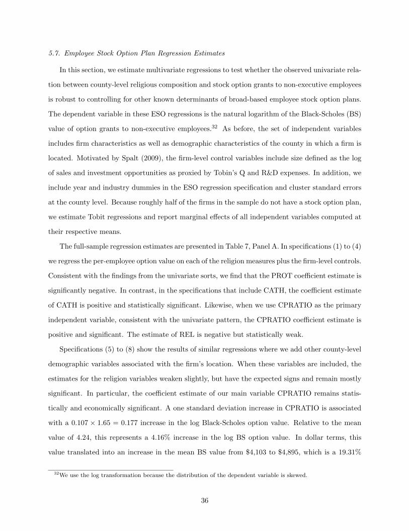
5.7. Employee Stock Option Plan Regression Estimates
In this section, we estimate multivariate regressions to test whether the observed univariate rela-
tion between county-level religious composition and stock option grants to non-executive employees
is robust to controlling for other known determinants of broad-based employee stock option plans.
The dependent variable in these ESO regressions is the natural logarithm of the Black-Scholes (BS)
value of option grants to non-executive employees.32 As before, the set of independent variables
includes firm characteristics as well as demographic characteristics of the county in which a firm is
located. Motivated by Spalt (2009), the firm-level control variables include size defined as the log
of sales and investment opportunities as proxied by Tobin’s Q and R&D expenses. In addition, we
include year and industry dummies in the ESO regression specification and cluster standard errors
at the county level. Because roughly half of the firms in the sample do not have a stock option plan,
we estimate Tobit regressions and report marginal effects of all independent variables computed at
their respective means.
The full-sample regression estimates are presented in Table 7, Panel A. In specifications (1) to (4)
we regress the per-employee option value on each of the religion measures plus the firm-level controls.
Consistent with the findings from the univariate sorts, we find that the PROT coefficient estimate is
significantly negative. In contrast, in the specifications that include CATH, the coefficient estimate
of CATH is positive and statistically significant. Likewise, when we use CPRATIO as the primary
independent variable, consistent with the univariate pattern, the CPRATIO coefficient estimate is
positive and significant. The estimate of REL is negative but statistically weak.
Specifications (5) to (8) show the results of similar regressions where we add other county-level
demographic variables associated with the firm’s location. When these variables are included, the
estimates for the religion variables weaken slightly, but have the expected signs and remain mostly
significant. In particular, the coefficient estimate of our main variable CPRATIO remains statis-
tically and economically significant. A one standard deviation increase in CPRATIO is associated
with a 0.107 × 1.65 = 0.177 increase in the log Black-Scholes option value. Relative to the mean
value of 4.24, this represents a 4.16% increase in the log BS option value. In dollar terms, this
value translated into an increase in the mean BS value from $4,103 to $4,895, which is a 19.31%
32We use the log transformation because the distribution of the dependent variable is skewed.
36

increase.33
In the next set of tests, we examine whether the religion variables proxy for other neighborhood
factors such as local labor market characteristics and social interaction effects that are known to
influence option grants to non-executive employees (Kedia and Rajgopal, 2009). Motivated by
their study, we enhance the ESO regression specification by including five neighborhood variables
that are measured for the metropolitan statistical area (MSA). Specifically, the tight labor market
dummy is set to one if the MSA unemployment rate is higher than the average MSA employment
rate; Local beta is the firm’s exposure to a local return index, which is computed using the Pirinsky
and Wang (2006) method; State-level non-compete enforceability index is from Garmaise (2010);
Market-adjusted MSA return is the median 12-month return of all firms headquartered in the MSA;
Industry cluster dummy is set to one for firms that are located in MSAs with an industry cluster;34
and Option grants at other firms in the MSA is the average Black-Scholes value of option grants
at other firms located in the MSA.
The regression estimates from the extended specifications are presented in Table 7, Panel B.
To facilitate comparison with prior results, in columns (1) and (3), we report estimates from
specifications similar to those used in the Kedia and Rajgopal (2009) study.35 Consistent with
their evidence, we find that non-executive option grant levels are higher among firms that have
higher local betas, are located in MSAs in which option grants are more common, or are located
in states with weaker non-compete agreements. Further, similar to their results, the unreported
demographic variable estimates indicate that more options are granted to non-executives in firms
located in counties with more educated individuals.
When we include CPRATIO in the regression specification (see columns (2) and (4)), it has a
significantly positive coefficient estimate. The estimates of neighborhood variables remain quali-
tatively similar, although the statistical significance of some variables weaken. In particular, the
33The new value of the option grant is computed as exp(ln(4103)+0.177) = $4,895.34We use the same definition of industry cluster as in Kedia and Rajgopal (2009). It is an MSA-level dummy
variable that takes a value of one if an industry makes up more than 10% of the MSA’s market capitalization andfirms from that industry in that MSA make up more than 10% of the industry’s total market capitalization. Industriesare based on two-digit SIC codes.
35Our empirical method is slightly different from Kedia and Rajgopal (2009). Unlike their study, we use a Tobitspecification and use the Black-Scholes value of option grants per employee instead of number of option grants scaledby shares outstanding.
37

coefficient estimate of “Option grants at other firms in the MSA” becomes insignificant. We also es-
timate the ESO regression separately for low and high CPRATIO sub-samples (see columns (5) and
(6)) and find that neighborhood variables have significant estimates only in the high CPRATIO sub-
sample. This evidence indicates that neighborhood factors have a stronger effect on non-executive
option grants when the local Catholic concentration is higher and the Protestant concentration is
lower.
The ESO regression estimates from these extended specifications indicate that prevalence of
certain religious beliefs could drive the social interaction effects that are known to influence option
grants. In particular, the local “culture” might be shaped by the religious composition of that
region, which in turn could influence the option grant policies of all firms located in the region. To
further examine the sensitivity of our baseline results, we consider an alternative measure of option
grants (the annual number of stock option grants per employee) and an alternative estimation
method (OLS instead of Tobit). For this estimation, we only consider the subsample of firms that
have an employee stock option plan. We find that our results are not affected by using these
alternative specifications (see Table 7, Panel B). Overall, the results from the ESO regressions are
consistent with our hypothesis H2a, which conjectures that religion-induced gambling attitudes
influence stock option grants to non-executive employees.
Similar to our previous analysis of institutional stock holdings, we look for further confirmation
that the observed effect of religion measures is due to their influence on gambling attitudes. We
first re-estimate the ESO regression for volatility-based subsamples. Each year we divide firms into
high and low subsamples based on the median level of volatility, which is reported as Sigma in
ExecuComp and is computed using the monthly stock returns over the prior 60 months. As the
return volatility of the underlying stock increases, stock options are likely to become increasingly
attractive to employees with preference for skewness. Thus, our proxies for gambling preferences
should yield stronger results in the high volatility subsample.
The subsample results are summarized in Table 7, Panel C. Consistent with our second employee
gambling preference hypothesis (H2b), we find that the coefficient estimates of PROT, CATH and
CPRATIO are all statistically significant in the high volatility subsample but insignificant or weaker
in the low volatility subsample. We find similar results when we consider size-based subsamples. In
particular, the CPRATIO coefficient estimate is stronger for the small firms subsample for which
38

local cultural factors are more likely to influence option grant policies and the headquarter location
would be a good proxy for the location of the majority of the workforce.
We also form subsamples based on county-level measures of income and education. The moti-
vation for this exercise is that the relation between the Black-Scholes value of non-executive option
grants and the religion variables would be stronger in counties in which the average county popula-
tion characteristics reflect employee characteristics more accurately. Compared to non-employees,
firm employees are likely to possess higher education levels and earn higher salaries. Thus, the cross-
sectional relation is expected to be stronger in the high education and high income sub-samples.
Consistent with this conjecture, we find that the coefficient estimates of the religion variables are
stronger in the high education and high income samples, while weak and insignificant in the low
income and low education subsamples.
5.8. Robustness of Employee Stock Option Plan Regressions
We examine the robustness of these ESO results using several additional tests. The results from
these robustness tests are summarized in Table 8, Panel A, where as before, for brevity, we focus
on the CPRATIO estimates. To begin, as with the institutional investor holdings regressions, we
control for the level of religiosity in our CPRATO regressions and find qualitatively similar results.
When we adopt a two-stage least squares approach using lagged values of the religion variables as
instruments, we find that the OLS and 2SLS results are very similar. The results are also robust
when we do not include industry dummies, use the CPDIFF measure instead of CPRATIO, and
extend the definition of PROT and CATH to include Mormons and Jews, respectively.
Our main results remain significant when we include additional control variables such as con-
temporaneous stock return, past two-year stock return, industry volatility, earnings volatility, and
measures of cash constraints (cash balances, cash dividends, cash flow and leverage). Additionally,
we find consistent results when we follow Oyer and Schaefer (2004) to define an indicator variable
for the existence of an ESO plan and then estimate logit regressions. To control for the differences
in option granting policies at the firm-level or differences in fairness concerns, we include the Black-
Scholes value of options granted to the CEO as an additional control variable and find that the
CPRATIO estimate remains significant.
The results are robust across time periods and in various geography-based subsamples. When we
39

do not use interpolated religion data and estimate cross-sectional ESO regressions for the year 1993
(the first year with the ESO data) and year 2000 only, we find that CPRATIO still has significantly
positive estimates. We find that the results remain significant when we exclude technology firms,
which are more likely to offer stock option plans to their employees. We also find that the results
are unchanged when we include the Republican state dummy, or a measure of social capital and
trust.36
In the last set of robustness tests, we estimate state and county fixed effects regressions using the
Rajan and Zingales (1998) method to further investigate the possibility that omitted geographical
variables drive our ESO results. In these regressions, we examine whether high volatility firms
grant more employee stock options if they are located in a region where the local population has
a higher propensity to gamble. We consider the high volatility measure in the Rajan and Zingales
(1998) type regressions because high volatility firms are more likely to be perceived as gambles by
employees due to their higher skewness (Spalt (2009)). We examine the within-state and within-
county differences between high and low volatility firms by defining an interaction variable between
one of the religion variables and the high volatility dummy. Our key conjecture is that the difference
in ESO grants between high and low volatility firms would be greater among firms located in high
CPRATIO regions.37
The results from the state fixed effects regressions presented in Table 8, Panel B are consistent
with our conjecture. The coefficient estimates of interaction terms defined using PROT, CATH,
and CPRATIO are all significant and have the correct signs. These estimates are also significant
economically. For example, increasing CPRATIO by one standard deviation for a firm with above
36To better establish the causal relation between regional religious composition and broad-based option grants,we collected data on headquarter location changes. We wanted to examine whether the option grant policy changeswhen a firm moves from a Catholic region to a Protestant region, and vice versa. Unfortunately, although there are195 moves during the ESO sample period, there are only 15 matches with the set of firms in the ESO sample. Thesmall number of matches prevents us from conducting any meaningful statistical analysis.
37We estimate these regressions using OLS on the subsample of firms that grant employee stock options. Becausethe Rajan and Zingales (1998) method involves the use of fixed effects, we estimate OLS regressions on the firm-year observations with positive option grants instead of the Tobit model that we use in our baseline specifications.We do not estimate ESO regressions using Tobit when the model has interaction terms because of the well-knownincidental parameters problem associated with non-linear panel data models, which would make our estimates biasedand inconsistent (Neyman and Scott, 1948; Lancaster, 2000). Further, when we estimate the ESO model with such alarge number of indicator variables and interaction, we face practical problems with difficulty of convergence in manycases. For example, our Tobit estimation procedure with state, year, and industry dummies does not converge whenwe focus on small or large firm subsamples.
40

median stock return volatility increases the number of granted options by 0.057 × 1.65 × 100 =
9.41%.38 To further test the robustness of our prediction, we estimate the state fixed effects
regression separately for the subset of small and large firms. Each year, we define small (large)
firms as those with below (above) median annual sales. Since we assign firms to counties and states
by the location of their headquarters, our estimates are likely to be more precise for small firms.
Consistent with this conjecture, we find that interaction term estimates have larger magnitudes
and are statistically more significant for the subsample of small firms.
When we estimate the ESO regressions using county fixed effects, all coefficient estimates have
the expected signs and they are similar in magnitudes to the state effects regressions, but only the
estimate of CATH is significant. The weak statistical significance is not surprising because there
is limited within-county variation in the option grant policies as there are an average of only 1.7
firms with ESO plan per county-year.
When we split the sample into large and small firms and re-estimate the county fixed effects
regressions, we again find that the estimates are stronger and consistent with our gambling hypothe-
ses for the subsample of small firms. All interaction terms are statistically significant for the small
firms subsample. In economic terms, the coefficient estimate of the CPRATIO interaction term
implies that the difference in stock option grants between small firms with high and low volatility
in a county that is at the 75th CPRATIO percentile is (1.63 − 0.25) × 0.071 × 100 = 9.94% higher
than the corresponding difference in a county that is at the 25th CPRATIO percentile.39
Collectively, the results from these robustness tests indicate that our baseline ESO regression
estimates are robust. We also find strong support for our second ESO hypothesis (H2b). Further,
we demonstrate that the impact of local religious composition on stock option grant policies is
unlikely to be driven by unobserved factors at the state or county levels.
38To be conservative, we assume in this calculation that the statistically insignificant coefficient estimate of CPRA-TIO is zero.
39An alternative explanation for higher ESO grants in high CPRATIO regions is that the Protestant work ethicmight provide more intrinsic motivation to Protestants (Weber, 1905, 1956), while Catholics need stronger incentivesdue to their lower intrinsic motivation. The volatility interaction results are inconsistent with this explanation becauseit is not clear why the intrinsic motivation levels of Catholics and Protestants would systematically vary across highand low volatility firms. The intrinsic motivation hypothesis can only be valid if less motivated Catholics and moremotivated Protestants systematically sort into high volatility firms within counties. While we cannot definitively ruleout this possibility, it is not obvious why such a systematic pattern would arise.
41

5.9. First-Day IPO Return and Turnover Regression Estimates
To test our third set of hypotheses, we use the first-day IPO return as the dependent variable.
The set of independent variables includes the religion measures, the county level demographic
characteristics, and the following determinants of initial day return identified in the recent IPO
literature (e.g., Purnanandam and Swaminathan, 2004; Loughran and Ritter, 2004; Cliff and Denis,
2004): (i) the size of the offering, defined as the natural logarithm of the total IPO proceeds; (ii) the
Carter and Manaster (1990) rating of the lead underwriter as a proxy for underwriter reputation;40
(iii) the gross spread charged by the underwriter; (iv) offer price revision, defined as the percentage
revision between the mid-point of the initial filing price range and the final offer price; (v) a
technology dummy that is set to one for a technology firm; (vi) the average daily return of the
CRSP value-weighted index over the three week period prior to the IPO offer date; and (vii) the
age of the issuing firm, defined as the natural logarithm of one plus the number of years since the
founding date. We estimate OLS regressions with year and industry dummies and cluster standard
errors at the county level.
The estimation results are presented in Table 9, Panel A. In specifications (1) to (4) of Panel A,
the dependent variable is the first-day IPO return. We find that the coefficient estimates of PROT
and CATH have the correct signs but they are not statistically significant. The coefficient estimate
of our key religion variable CPRATIO, however, is significant both statistically and economically.
A one standard deviation increase in CPRATIO corresponds to a 0.526×1.65 = 0.87% higher first-
day return. Relative to the mean first-day return of 16.55%, this is a 5.24% increase. Further, there
is a 1.40 standard deviation difference between the CPRATIO levels across the extreme quartiles.
Thus, IPOs offered in counties that are in the two extreme CPRATIO quintiles would have an
average first-day return differential of 0.526 × 1.40 × 1.65 = 1.22%. These estimates indicate that
differences in religious composition across counties have an economically significant influence on
the first-day IPO return.
In addition to the first-day return, we examine the effect of local religion on the first-day IPO
turnover in specifications (5) to (8) of Table 9, Panel A. First-day turnover can be interpreted as an
alternative measure of speculative interest in an issuing firm’s stock. We expect the religion-first-
40When there are multiple lead underwriters, we use their average reputation.
42

day turnover relation to be similar to the religion-first-day return relation. Consistent with this
conjecture, we find that the results from turnover regressions are qualitatively similar to those from
the return regressions, although the statistical significance is weaker. PROT is negatively related to
first-day turnover, while CATH and CPRATIO are positively related to turnover. Taken together,
the first-day return and turnover regression results are consistent with our first IPO hypothesis
(H3a).
To test the second IPO hypothesis (H3b), which posits that high local market participation and
strong local bias would amplify the relation between religion and first-day returns, we re-estimate
the IPO regressions for various market participation, retail clientele, and local bias subsamples.
Motivated by the evidence in Campbell (2006), we use income and education as proxies for stock
market participation. For the 1998 to 2005 period, we consider another state-level stock market
participation proxy that has been proposed in Brown et al. (2007). It is defined as the proportion
of tax returns in each state that reports dividend income on IRS tax returns.
We also partition the sample based on offer price and first-day turnover to focus on IPOs
in which retail investors are more likely to participate and influence the first-day return. Retail
investors are known to prefer low-priced stocks (e.g., Kumar, 2009) and high initial turnover is
likely to be a rough indicator of the degree to which investors with initial allocations of the IPO
“flip” the shares to retail or other investors. To capture the incremental effects of local bias, we
obtain state-level measures of local bias using the retail brokerage data and examine subsamples
based on this retail local bias measure.41
The IPO subsample results are summarized in Table 9, Panel B. We find that the coefficient
estimates of religion variables are stronger in high income, high education, and high market partici-
pation subsamples. Consistent with our conjecture, we also find that the IPO regression results are
stronger in the low price, small size, and high turnover IPO subsamples. Further, even with a coarse
state-level measure of local bias, we find that the effect of religion measures is notably stronger in
the high local bias subsample. When we examine subsamples formed on both market participation
41The local bias measure is defined as LB = 1 − Dact/Dportf , where Dact is the average distance between aninvestor’s location and stocks in her portfolio, while Dportf is the average distance between an investor’s locationand other characteristic-matched portfolios not held by the investor. The state-level local bias measure is an equal-weighted average of the local bias of brokerage investors located in the state.
43

proxy (income) and local bias, we find that the results are strongest in the high income, high local
bias subsample. These results provide strong support for our second local bias hypothesis (H3b)
and indicate that the effect of religion on first-day return is stronger among IPOs with stronger
retail clientele and when local stock market participation rate and local bias are high.
5.10. Robustness of IPO Regression Regressions
We perform several robustness checks similar to those in the previously discussed settings.
These results are presented in Table 10, Panel A. We find that IPO regression results are stronger
when we control for the degree of religiosity in the county. The results remain strong when we use
an instrumental variables specification with a lagged religion variable. The results are also robust
when we exclude industry dummies, use the CPDIFF measure instead of CPRATIO, or extend the
religion variables to include Mormons and Jews. When we use state lottery sales as an independent
variable, we find that it has a weak positive effect. However, its estimate is no longer significant
when we include CPRATIO in the regression specification.
The subperiod estimates indicate that the IPO regression estimates are strong in the latter part
of the sample and weak in the early half of the sample. The results are mostly robust in the various
geography-based subsamples. The results are weak when California or the West Census region are
excluded, but the results in these geographic subsamples improve considerably in the latter sample
period or when we focus on the high retail bias subsample. The IPO results are unlikely to be
driven by unobserved factors at the state level because when we include state-level controls for
political preferences, social capital, and trust, the CPRATIO coefficient remains significant.
As in the previous settings, we use the Rajan and Zingales (1998) estimation method to further
ensure that our results are robust to unobserved geographical heterogeneity at the county and state
levels. In both county and state fixed effects regressions, we find a positive coefficient estimate for
the interaction between CPRATIO and the technology firm dummy. Consistent with our gambling
hypothesis, this evidence indicates that the first-day return for technology stocks is significantly
higher if the company is located in a high CPRATIO county. This effect is stronger in regions
with stronger local bias, which again supports our conjecture that local gambling attitudes affect
first-day IPO return.
Using counties in the extreme quartiles to illustrate the economic significance of the IPO results,
44

we find that the difference between the mean first-day IPO return for technology firms and other
firms is (1.63 − 0.25) × 1.158 = 1.62% higher in a county with CPRATIO at the 75th percentile
than in a county with CPRATIO at the 25th percentile. Relative to the mean first-day return of
16.55%, this reflects a 9.79% difference. These differences are even more pronounced in high local
bias regions or when we estimate the IPO regressions using county fixed effects.
Overall, these robustness test results provide strong support for our conjecture that religion-
induced gambling preferences of local individuals affect first-day return and turnover of local IPOs.
We are also able to establish that these effects are unlikely to be driven by unobserved geographical
heterogeneity.
5.11. Lottery Stock Premium: Fama-MacBeth Regression Estimates
In the last part of the paper, we estimate Fama-MacBeth regressions to estimate the lottery-
stock premium and gather support for our fourth hypothesis (H4). We modify the primary re-
gression specification used in Kumar (2009) to estimate the lottery-type stock premium. This
specification is very similar to the specification used in Ang et al. (2009) to examine the pricing of
idiosyncratic volatility.
The dependent variable in these regressions is the monthly stock return, while the set of in-
dependent variables includes several stock characteristics and factor exposures as well as religion
related variables. The primary independent variable is the Lottery Stock × High Religion interac-
tion term, where one of the four religion variables (PROT, CATH, CPRATIO, or REL) is used to
define the interaction variable. The High Religion dummy is set to one for firms that are located
in regions in which the religion measure is above its median value. Our main conjecture is that the
negative lottery stock premium would be more negative when a firm is located in a high CPRATIO
region. Therefore, the interaction variable defined using PROT should have a significantly posi-
tive estimate, while the CATH and CPRATIO interaction terms should have significantly negative
estimates.
The Fama-MacBeth regression results for the 1980 to 2005 sample period are reported in Table
11, Panel A. When the religion interaction is not included in the specification, the lottery stock
dummy has a significantly negative coefficient estimate. The estimate of −0.125 (t-statistic =
−3.52) translates into an annualized average lottery stock underperformance of 0.125×12 = 1.50%.
45

When we include Lottery Stock × PROT interaction term in the specification, consistent with our
hypothesis, we find that it has a significantly positive sign. Similarly, the CATH interaction term
has a marginally negative coefficient estimate and CPRATIO has a strongly negative estimate.
In economic terms, these estimates indicate that when the local clientele exhibits a preference
for lottery-type stocks due to their religious background, the lottery-type stocks earn significantly
lower average return. For instance, when the CPRATIO in a region is above its median, lottery-
type stocks underperform by an additional 0.053 × 12 = 0.64% on an annual basis. The average
annualized underperformance increases from 1.50% to 2.14%. In contrast, when the PROT measure
is above its median value, lottery-type stocks earn 0.058 × 12 = 0.70% higher average annualized
return. The average annualized underperformance of lottery type stocks drops from 1.50% to 0.80%.
Our robustness check results reported in Table 11, Panel B indicate that the incremental effect
of CPRATIO on the lottery stock premium is robust. We find that Lottery Stock × High CPRA-
TIO interaction term remain significant when we use the CPDIFF measure instead of CPRATIO,
extend the religion variables to include Mormons and Jews, use characteristic-adjusted return to
measure performance, consider sub-periods, or consider geographic subsamples. The interaction
estimates also remain qualitatively similar when we introduce additional regional controls such as
the Republican state dummy and measures of social capital and trust. Taken together, these results
support our lottery-stock premium hypothesis (H4) and indicate that the magnitude of the nega-
tive lottery stock premium is incrementally affected by the religious characteristics and gambling
propensity of local investors.
6. Summary and Conclusion
We use religious background as a proxy for gambling propensity and examine whether geograph-
ical variation in religion-induced gambling norms affects aggregate market outcomes. We focus on
four distinct economic settings in which the existing literature has suggested a role for gambling and
speculative behavior. Our results indicate that in regions with higher concentration of Catholics
relative to Protestants, institutions hold larger lottery-type stock portfolios, non-executive employ-
ees receive larger stock option grants, the initial day IPO return is higher, and the magnitude of
the negative lottery stock premium is higher. These seemingly unrelated findings are driven by a
46

common gambling-based mechanism. Operating through this gambling channel, religion influences
investors’ portfolio choices, corporate decisions, and stock returns.
The consistency in the relation between local religious composition and aggregate market out-
comes in multiple settings provides strong support to our gambling-related hypotheses and high-
lights the important role of gambling in understanding aggregate market outcomes. In broader
terms, our empirical evidence contributes to the emerging literature in economics that examines
the interplay between culture and economic outcomes. Because religion is one of the key cultural
attributes, our results indicate that through an influence on gambling attitudes, cultural norms
may impact financial markets more strongly than previously believed.
Our study focuses on economic settings in which the existing literature has already suggested a
possible role of gambling and speculation. However, the remarkable similarities in our results across
different economic settings indicate that religious beliefs might be important in other economic
settings and could have an even stronger influence on financial markets. For example, recent
studies in corporate finance indicate that managerial incentives affect corporate policies. It is likely
that when offered similar contracts, the religious background of a manager determines her response
to performance-based incentives. Therefore, through its effect on ethics and values, differences in
religious beliefs could have a significant effect on corporate policies, including capital structure
choices.
47

References
Alesina, A., La Ferrara, E., 2000. Participation in heterogeneous communities. Quarterly Journal
of Economics 115, 847–904.
Ang, A., Hodrick, R.J., Xing, Y., Zhang, X., 2009. High idiosyncratic volatility and low returns:
International and further U.S. evidence. Journal of Financial Economics 91, 1–23.
Badrinath, S.G., Gay, G.D., Kale, J.R., 1989. Patterns of institutional investment, prudence, and
the managerial “safety-net” hypothesis. Journal of Risk and Insurance 56, 605–629.
Baker, M., Bradley, B., Wurgler, J., 2011. Benchmarking as limits to arbitrage: Uunderstanding
the low volatility anomaly. Financial Analyst Journal 67, 40–54.
Barber, B.M., Odean, T., 2000. Trading is hazardous to your wealth: The common stock investment
performance of individual investors. Journal of Finance 55, 773–806.
Barberis, N., Huang, M., 2008. Stocks as lotteries: The implications of probability weighting for
security prices. American Economic Review 98, 2066–2100.
Barro, R.J., McCleary, R.M., 2003. Religion and economic growth across countries. American
Sociological Review 68, 760–781.
Becker, B., 2007. Geographical segmentation of U.S. capital markets. Journal of Financial Eco-
nomics 85, 151–178.
Becker, B., Ivkovich, Z., Weisbenner, S., 2010. Local dividend clienteles. Journal of Finance
Forthcoming.
Bennett, J.A., Sias, R.W., Starks, L.T., 2003. Greener pastures and the impact of dynamic insti-
tutional preferences. Review of Financial Studies 16, 1203–1238.
Bergman, N., Jenter, D., 2007. Employee sentiment and stock option compensation. Journal of
Financial Economics 84, 667–712.
Berry, F.S., Berry, W.D., 1990. State lottery adoptions as policy innovations: An event history
analysis. Amerian Political Science Review 84, 395–415.
48

Brown, J.R., Ivkovic, Z., Smith, P.A., Weisbenner, S., 2007. Neighbors matter: Causal community
effects and stock market participation. Journal of Finance 63, 1509–1531.
Brown, K.C., Harlow, W., Starks, L.T., 1996. Of tournaments and temptations: An analysis of
managerial incentives in the mutual fund industry. Journal of Finance 51, 85–110.
Bushee, B.J., 1998. The influence of institutional investors on myopic r&d investment behavior.
Accounting Review 73, 305–333.
Campbell, J.Y., 2006. Household finance. Journal of Finance 61, 1553–1604.
Carter, R.B., Manaster, S., 1990. Initial public offerings and underwriter reputation. Journal of
Finance 45, 1045–1067.
Cliff, M.T., Denis, D., 2004. Do initial public offering firms purchase analyst coverage with under-
pricing? Journal of Finance 59, 2871–2901.
Clotfelter, C.T., Cook, P.J., 1989. Selling Hope: State Lotteries in America. Harvard University
Press, Cambridge, MA.
Coughlin, C.C., Garrett, T.A., 2008. Income and lottery sales: Transfers trump income from
work and wealth. FRB of St. Louis Working Paper No. 2008-004C; Available at SSRN:
http://ssrn.com/abstract=1084183.
Daniel, K.D., Grinblatt, M., Titman, S., Wermers, R., 1997. Measuring mutual fund performance
with characteristic-based benchmarks. Journal of Finance 52, 1035–1058.
Darnell, A., Sherkat, D.E., 1997. The impact of protestant fundamentalism on educational attain-
ment. American Sociological Review 62, 306–315.
Del Guercio, D., 1996. The distorting effect of the prudent man law on institutional equity invest-
ments. Journal of Financial Economics 40, 31–62.
Desai, M., 2003. The divergence between book and tax income. Tax Policy and the Economy 17,
169–206. James Poterba (Editor), MIT Press, Cambridge, MA.
Devers, C., Wiseman, R., Holmes, M., 2007. The effects of endowment and loss aversion in man-
agerial stock option valuation. Academy of Management Journal 50, 191–208.
49

Diaz, J.D., 2000. Religion and gambling in sin-city: A statistical analysis of the relationship between
religion and gambling patterns in Las Vegas residents. Social Science Journal 37, 3.
Doran, J.S., Jiang, D., Peterson, D.R., 2011. Gambling in the new year? The January idiosyncratic
volatility puzzle. Review of Finance Forthcoming.
Dorn, D., Sengmueller, P., 2009. Trading as entertainment. Management Science 55, 591–603.
Ellison, C.G., Nybroten, K.A., 1999. Conservative protestantism and opposition to state-sponsored
lotteries: Evidence from the 1997 Texas poll. Social Science Quarterly 80, 356–369.
Fama, E.F., French, K.R., 1997. Industry costs of capital. Journal of Financial Economics 43,
153–193.
Garmaise, M.J., 2010. Ties that truly bind: Non-competition agreements, executive compensation
and firm investment. Journal of Law, Economics, and Organization Forthcoming.
Glaeser, E.L., Ward, B.A., 2006. Myths and realities of American political geography. Working
Paper, Harvard Business School.
Grichting, W.L., 1986. The impact of religion on gambling in Australia. Australian Journal of
Psychology 38, 45–58.
Grinblatt, M., Keloharju, M., 2009. Sensation seeking, overconfidence, and trading activity. Journal
of Finance 64, 549–578.
Guiso, L., Sapienza, P., Zingales, L., 2003. People’s opium? Religion and economic attitude.
Journal of Monetary Economics 50, 225–282.
Guiso, L., Sapienza, P., Zingales, L., 2006. Does culture affect economic outcomes? Journal of
Economic Perspectives 20, 23–48.
Guiso, L., Sapienza, P., Zingales, L., 2008. Trusting the stock market. Journal of Finance 63,
2557–2600.
Hallock, K., Olson, C., 2006. The value of stock options to non-executive employees. NBER
Working Paper 11950.
50

Hilary, G., Hui, K.W., 2009. Does religion matter in corporate decision making in America? Journal
of Financial Economics 93, 455–473.
Hodge, F., Rajgopal, S., Shevlin, T., 2010. Do managers value stock options and restricted stock
consistent with economic theory? Contemporary Accounting Research 26, 899–932.
Hoffman, J.P., 2000. Religion and problem gambling in the U.S. Review of Religious Research 41,
488–509.
Hong, H., Scheinkman, J.A., Xiong, W., 2006. Asset float and speculative bubbles. Journal of
Finance 61, 1073–1117.
Iannaccone, L.R., 1998. Introduction to the economics of religion. Journal of Economic Literature
36, 1465–1495.
Kallick, M., Smits, D., Dielman, T., Hybels, J., 1979. A survey of American gambling attitudes
and behavior. Survey Research Center Research Report, Institute for Social Research, University
of Michigan.
Kedia, S., Rajgopal, S., 2009. Neighborhood matters: The impact of location on broad based stock
option plans. Journal of Financial Economics 92, 109–127.
Keister, L.A., 2003. Religion and wealth: The role of religious affiliation and participation in early
adult asset accumulation. Social Forces 82, 175–207.
Keister, L.A., 2007. Upward wealth mobility: Exploring the roman catholic advantage. Social
Forces 85, 1195–1225.
Kumar, A., 2009. Who gambles in the stock market? Journal of Finance 64, 1889–1933.
Lancaster, T., 2000. The incidental parameter problem since 1948. Journal of Econometrics 95,
391–413.
Lehrer, E.L., 1998. Religious intermarriage in the united states: Determinants and trends. Social
Science Research 27, 245–263.
Lehrer, E.L., 1999. Religion as a determinant of educational attainment: An economic perspective.
Social Science Research 28, 358–379.
51

Lehrer, E.L., 2009. The role of religion in economic and demographic behavior in the united states:
A review of the recent literature. IZA Discussion Paper No. 3541.
Lehrer, E.L., Chiswick, C.U., 1993. Religion as a determinant of marital stability. Demography 30,
385–404.
Lewellen, J., 2011. Institutional investors and the limits of arbitrage. Journal of Financial Economics
Forthcoming.
Loughran, T., Ritter, J., 2004. Why has IPO underpricing changed over time? Financial Manage-
ment 33, 5–37.
Markowitz, H., 1952. The utility of wealth. Journal of Political Economy 60, 151–158.
Martin, R., Yandle, B., 1990. State lotteries as duopoly transfer mechanisms. Public Choice 64,
253–264.
Neyman, J., Scott, E.L., 1948. Consistent estimation from partially consistent observations. Econo-
metrica 16, 1–32.
Oyer, P., Schaefer, S., 2004. Why do some firms give stock options to all employees? An empirical
examination of alternative theories. Journal of Financial Economics 76, 99–133.
Ozment, S., 1991. Protestant: The Birth of a Revolution. Doubleday, New York, NY.
Pirinsky, C., Wang, Q., 2006. Does corporate headquarters location matter for stock returns?
Journal of Finance 61, 1991–2015.
Pontiff, J., 1996. Costly arbitrage: Evidence from closed-end funds. Quarterly Journal of Economics
111, 1135–1151.
Purnanandam, A., Swaminathan, B., 2004. Are IPOs really underpriced? Review of Financial
Studies 17, 811–848.
Putnam, R.D., 2000. Bowling Alone: The Collapse and Revival of American Community. Simon
and Schuster, New York, NY.
52

Rajan, R.G., Zingales, L., 1998. Financial dependence and growth. American Economic Review
88, 559–586.
Scheinkman, J.A., Xiong, W., 2003. Overconfidence and speculative bubbles. Journal of Political
Economy 111, 1183–1219.
Shiller, R.J., 2000. Irrational Exuberance. Princeton University Press, Princeton, NJ.
Spalt, O.G., 2009. Probability weighting and employee stock options. Working Paper (November),
Tilburg University; Available at SSRN: http://ssrn.com/abstract=1102947.
Starkey, L.M., 1964. Money, Mania, and Morals: The Churches and Gambling. Abingdon Press,
New York, NY.
Stulz, R.M., Williamson, R., 2003. Culture, openness, and finance. Journal of Financial Economics
70, 313–349.
Thompson, W.N., 2001. Gambling in America: An Encyclopedia of History, Issues, and Society.
ABC-CLIO, Inc.
Weber, M., 1905, 1956. The Protestant Ethic and The Spirit of Capitalism. Unwin University
Books, London, UK.
53

Table 1Summary Statistics
This table presents summary statistics for the various data sets used in the paper. Panel A presents county-
level summary statistics of religion variables and demographic characteristics for all US counties with com-
plete data. Protestants (PROT) is the proportion of Protestant adherents in a county, Catholics (CATH)
is the proportion of Catholic adherents in a county, Catholic-Protestant Ratio (CPRATIO) is the ratio of
Catholics to Protestants, and Religiosity (REL) is the proportion of county population that adheres to any
religion. Income is the median household income in a county. Total population is the total county-level
population in millions. Education is the proportion of county-level population over the age of 25 with a
bachelor’s degree or higher. Male-Female Ratio is the ratio of male to female residents in a county. Married
is the proportion of county households with a married couple. Minority is the proportion of county residents
who are non-white. Age is the median age of county residents. Urban is the proportion of county population
that lives in urban areas. Panel B presents the county-level summary statistics for the counties in the institu-
tional dataset. Panel C shows pooled sample summary statistics of institutional portfolio attributes covering
the 1980 to 2005 period. Lottery stocks are defined as stocks with above-median idiosyncratic volatility
and above-median idiosyncratic skewness levels, while non-lottery stocks have below median volatility and
skewness levels. The volatility and skewness measures are computed using past six months of daily returns.
(Non-) Lottery-Stock Weight is the fraction of the portfolio holdings that is allocated to (non-) lottery-type
stocks. IPO Weight is the average portfolio weight allocated to all firms that went public in the previous
quarter. Non-local IPOs are located at least 250 miles away from the location of the institution. Portfolio
Size is the market value of the total institutional equity portfolio and Portfolio Concentration is the Herfind-
ahl index computed using the portfolio weights. The number of institutions per county-quarter is presented
as summary statistics on the county level. Panel D shows pooled sample summary statistics for the employee
stock option plan sample covering the 1992 to 2005 period. ESO Plan is the percentage of firms with an
employee stock option plan. Options-Shares Ratio is the ratio of stock options granted to the number of
shares outstanding. BS Value per Employee is the Black-Scholes value of non-executive stock options granted
divided by the number of non-executive employees in the firm and BS Value CEO is the Black-Scholes value
of options granted to the firm’s CEO. Sales is the dollar-value of annual firm sales. Tobin’s Q is calculated
as book assets minus book equity plus market value of equity, scaled by total assets. R&D is the three
year average of research and development expense scaled by total assets. Panel E presents pooled sample
summary statistics for IPOs offered during the 1980 to 2005 period. First-Day Return is the return from
the offer price to the closing price on the first day of trading. First-Day Turnover is the turnover on the
first trading day. IPO Proceeds is the total capital raised by the firm through the IPO process. Underwriter
Rank is the Carter and Manaster (1990) rank of the lead manager. Underwriter Spread is the gross spread
charged by the underwriter as compensation for its underwriting services. Offer Price Revision is the price
change from the midpoint of the filing range to the offer price. Pre-IPO Market Return is the average daily
CRSP value-weighted market return during the three week period prior to the offer date. Firm Age is the
age of the firm relative to the founding date. Following Loughran and Ritter (2004), the Technology Firm
Dummy is set to one for IPOs with SIC codes between 3570 and 3579, 3661, 3674, 5045, 5961, or 7370 and
7379.
54

Table 1 – Continued from previous pageSummary Statistics
Panel A: County-Level Demographic Characteristics (All U.S. Counties)
Variable Mean MedianStdDev
10th
Pctl25th
Pctl75th
Pctl90th
Pctl N
PROT (%) 40.43 40.37 18.92 15.17 25.37 53.99 65.26 3,092CATH (%) 13.21 8.62 14.32 0.56 1.99 19.12 33.54 3,092CPRATIO 0.60 0.23 1.02 0.01 0.05 0.67 1.50 3,092REL (%) 56.83 55.86 17.61 34.68 43.93 68.84 81.28 3,092Income ($) 17,214 16,772 3,807 3,293 14,814 18,795 21,396 3,092Total Population (’000s) 83.38 23.46 272.34 5.38 10.92 58.40 158.42 3,092Education (%) 14.40 12.65 6.68 8.25 9.97 16.68 23.06 3,092Male-Female Ratio 97.57 96.48 7.09 91.73 93.84 99.38 103.62 3,092Married (%) 59.61 60.34 5.74 52.39 56.67 63.17 65.85 3,092Minority (%) 13.74 6.97 15.80 1.17 2.35 20.54 36.12 3,092Median Age (years) 35.05 35.05 3.67 30.70 32.96 37.17 39.48 3,092Urban (%) 37.59 36.60 29.21 0.00 10.17 58.89 80.61 3,092
Panel B: County-Level Demographic Characteristics (Counties with Institutions)
Variable Mean MedianStdDev
10th
Pctl25th
Pctl75th
Pctl90th
Pctl N
PROT (%) 27.62 24.95 14.40 10.56 15.85 37.03 49.40 415CATH (%) 20.01 17.44 14.75 3.62 7.73 27.82 40.91 415CPRATIO 1.29 0.68 1.65 0.08 0.25 1.63 3.25 415REL (%) 50.61 50.26 13.23 34.70 41.27 59.41 67.93 415Income ($) 25,676 24,613 8,860 15,246 20,385 29,603 37,598 415Total Population (’000s) 391.41 201.25 654.42 44.33 84.19 491.42 861.98 415Education (%) 24.35 22.97 9.97 12.60 17.11 29.47 38.85 415Male-Female Ratio 95.96 95.56 4.59 91.08 92.82 98.38 101.21 415Married (%) 53.87 53.73 7.56 46.05 49.51 58.97 63.25 415Minority (%) 18.11 14.57 14.42 3.26 7.01 26.24 38.36 415Median Age (years) 34.61 34.61 3.33 30.76 32.63 36.60 38.61 415Urban (%) 75.50 82.99 22.72 40.08 62.51 93.81 98.49 415
Panel C: Institutional Portfolio Characteristics
Variable Mean MedianStdDev
10th
Pctl25th
Pctl75th
Pctl90th
Pctl N
Lottery-Stock Weight(%) 9.49 5.09 12.69 0.25 1.83 12.12 23.96 101,377
Non-Lottery-StockWeight (%) 43.47 44.50 16.19 22.95 34.88 53.19 61.44 101,377
IPO Weight (%) 0.28 0.00 2.04 0.00 0.00 0.00 0.44 101,368Non-Local IPO Weight
(%) 0.17 0.00 1.39 0.00 0.00 0.00 0.16 101,368Portfolio Size ($m) 544.02 279.09 705.26 71.88 136.02 640.91 1,349.07 101,377Portfolio Concentration
(HHI) 0.07 0.03 0.15 0.01 0.02 0.05 0.12 101,377Institutions Per
County-Quarter 3.58 1.00 13.84 1.00 1.00 2.39 5.91 415
55
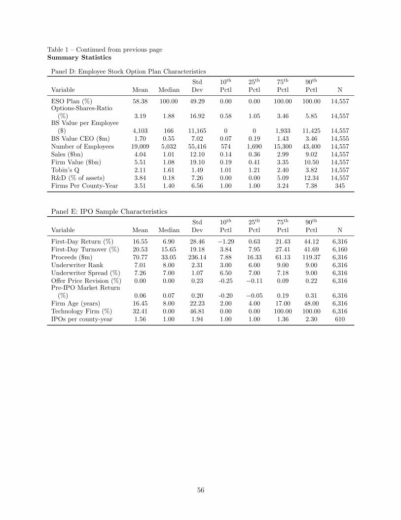
Table 1 – Continued from previous pageSummary Statistics
Panel D: Employee Stock Option Plan Characteristics
Variable Mean MedianStdDev
10th
Pctl25th
Pctl75th
Pctl90th
Pctl N
ESO Plan (%) 58.38 100.00 49.29 0.00 0.00 100.00 100.00 14,557Options-Shares-Ratio
(%) 3.19 1.88 16.92 0.58 1.05 3.46 5.85 14,557BS Value per Employee
($) 4,103 166 11,165 0 0 1,933 11,425 14,557BS Value CEO ($m) 1.70 0.55 7.02 0.07 0.19 1.43 3.46 14,555Number of Employees 19,009 5,032 55,416 574 1,690 15,300 43,400 14,557Sales ($bn) 4.04 1.01 12.10 0.14 0.36 2.99 9.02 14,557Firm Value ($bn) 5.51 1.08 19.10 0.19 0.41 3.35 10.50 14,557Tobin’s Q 2.11 1.61 1.49 1.01 1.21 2.40 3.82 14,557R&D (% of assets) 3.84 0.18 7.26 0.00 0.00 5.09 12.34 14,557Firms Per County-Year 3.51 1.40 6.56 1.00 1.00 3.24 7.38 345
Panel E: IPO Sample Characteristics
Variable Mean MedianStdDev
10th
Pctl25th
Pctl75th
Pctl90th
Pctl N
First-Day Return (%) 16.55 6.90 28.46 −1.29 0.63 21.43 44.12 6,316First-Day Turnover (%) 20.53 15.65 19.18 3.84 7.95 27.41 41.69 6,160Proceeds ($m) 70.77 33.05 236.14 7.88 16.33 61.13 119.37 6,316Underwriter Rank 7.01 8.00 2.31 3.00 6.00 9.00 9.00 6,316Underwriter Spread (%) 7.26 7.00 1.07 6.50 7.00 7.18 9.00 6,316Offer Price Revision (%) 0.00 0.00 0.23 -0.25 −0.11 0.09 0.22 6,316Pre-IPO Market Return
(%) 0.06 0.07 0.20 -0.20 −0.05 0.19 0.31 6,316Firm Age (years) 16.45 8.00 22.23 2.00 4.00 17.00 48.00 6,316Technology Firm (%) 32.41 0.00 46.81 0.00 0.00 100.00 100.00 6,316IPOs per county-year 1.56 1.00 1.94 1.00 1.00 1.36 2.30 610
56
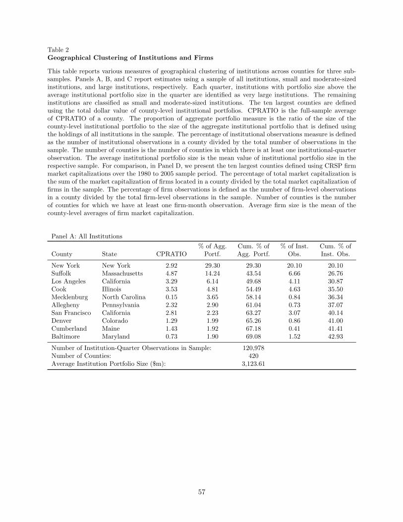
Table 2Geographical Clustering of Institutions and Firms
This table reports various measures of geographical clustering of institutions across counties for three sub-samples. Panels A, B, and C report estimates using a sample of all institutions, small and moderate-sizedinstitutions, and large institutions, respectively. Each quarter, institutions with portfolio size above theaverage institutional portfolio size in the quarter are identified as very large institutions. The remaininginstitutions are classified as small and moderate-sized institutions. The ten largest counties are definedusing the total dollar value of county-level institutional portfolios. CPRATIO is the full-sample averageof CPRATIO of a county. The proportion of aggregate portfolio measure is the ratio of the size of thecounty-level institutional portfolio to the size of the aggregate institutional portfolio that is defined usingthe holdings of all institutions in the sample. The percentage of institutional observations measure is definedas the number of institutional observations in a county divided by the total number of observations in thesample. The number of counties is the number of counties in which there is at least one institutional-quarterobservation. The average institutional portfolio size is the mean value of institutional portfolio size in therespective sample. For comparison, in Panel D, we present the ten largest counties defined using CRSP firmmarket capitalizations over the 1980 to 2005 sample period. The percentage of total market capitalization isthe sum of the market capitalization of firms located in a county divided by the total market capitalization offirms in the sample. The percentage of firm observations is defined as the number of firm-level observationsin a county divided by the total firm-level observations in the sample. Number of counties is the numberof counties for which we have at least one firm-month observation. Average firm size is the mean of thecounty-level averages of firm market capitalization.
Panel A: All Institutions
County State CPRATIO% of Agg.
Portf.Cum. % ofAgg. Portf.
% of Inst.Obs.
Cum. % ofInst. Obs.
New York New York 2.92 29.30 29.30 20.10 20.10Suffolk Massachusetts 4.87 14.24 43.54 6.66 26.76Los Angeles California 3.29 6.14 49.68 4.11 30.87Cook Illinois 3.53 4.81 54.49 4.63 35.50Mecklenburg North Carolina 0.15 3.65 58.14 0.84 36.34Allegheny Pennsylvania 2.32 2.90 61.04 0.73 37.07San Francisco California 2.81 2.23 63.27 3.07 40.14Denver Colorado 1.29 1.99 65.26 0.86 41.00Cumberland Maine 1.43 1.92 67.18 0.41 41.41Baltimore Maryland 0.73 1.90 69.08 1.52 42.93
Number of Institution-Quarter Observations in Sample: 120,978Number of Counties: 420Average Institution Portfolio Size ($m): 3,123.61
57
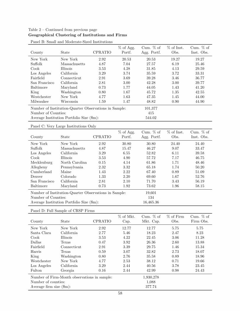
Table 2 – Continued from previous page
Geographical Clustering of Institutions and Firms
Panel B: Small and Moderate-Sized Institutions
County State CPRATIO% of Agg.
Portf.Cum. % ofAgg. Portf.
% of Inst.Obs.
Cum. % ofInst. Obs.
New York New York 2.92 20.53 20.53 19.27 19.27Suffolk Massachusetts 4.87 7.04 27.57 6.19 25.46Cook Illinois 3.53 4.28 31.85 4.13 29.59Los Angeles California 3.29 3.74 35.59 3.72 33.31Fairfield Connecticut 2.91 3.69 39.28 3.46 36.77San Francisco California 2.81 3.00 42.28 3.00 39.77Baltimore Maryland 0.73 1.77 44.05 1.43 41.20King Washington 0.80 1.67 45.72 1.35 42.55Westchester New York 4.77 1.63 47.35 1.45 44.00Milwaukee Wisconsin 1.59 1.47 48.82 0.90 44.90
Number of Institution-Quarter Observations in Sample: 101,377Number of Counties: 415Average Institution Portfolio Size ($m): 544.02
Panel C: Very Large Institutions Only
County State CPRATIO% of Agg.
Portf.Cum. % ofAgg. Portf.
% of Inst.Obs.
Cum. % ofInst. Obs.
New York New York 2.92 30.80 30.80 24.40 24.40Suffolk Massachusetts 4.87 15.47 46.27 9.07 33.47Los Angeles California 3.29 6.55 52.82 6.11 39.58Cook Illinois 3.53 4.90 57.72 7.17 46.75Mecklenburg North Carolina 0.15 4.14 61.86 1.71 48.46Allegheny Pennsylvania 2.32 3.32 65.18 1.74 50.20Cumberland Maine 1.43 2.22 67.40 0.89 51.09Denver Colorado 1.33 2.20 69.60 1.67 52.76San Francisco California 2.81 2.10 71.70 3.43 56.19Baltimore Maryland 0.73 1.92 73.62 1.96 58.15
Number of Institution-Quarter Observations in Sample: 19,601Number of Counties: 134Average Institution Portfolio Size ($m): 16,465.36
Panel D: Full Sample of CRSP Firms
County State CPRATIO% of Mkt.
Cap.Cum. % ofMkt. Cap.
% of FirmObs.
Cum. % ofFirm Obs.
New York New York 2.92 12.77 12.77 5.75 5.75Santa Clara California 2.77 5.46 18.23 2.47 8.23Cook Illinois 3.53 4.22 22.45 3.06 11.28Dallas Texas 0.47 3.92 26.36 2.60 13.88Fairfield Connecticut 2.91 3.39 29.75 1.46 15.34Harris Texas 0.59 3.07 32.82 2.73 18.07King Washington 0.80 2.76 35.58 0.89 18.96Westchester New York 4.77 2.53 38.12 0.71 19.66Los Angeles California 3.29 2.44 40.56 3.78 23.45Fulton Georgia 0.16 2.44 42.99 0.98 24.43
Number of Firm-Month observations in sample: 1,930,278Number of counties: 1,088Average firm size ($m): 377.74
58
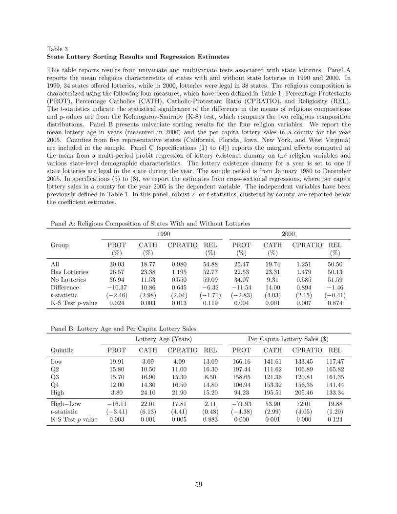
Table 3State Lottery Sorting Results and Regression Estimates
This table reports results from univariate and multivariate tests associated with state lotteries. Panel Areports the mean religious characteristics of states with and without state lotteries in 1990 and 2000. In1990, 34 states offered lotteries, while in 2000, lotteries were legal in 38 states. The religious composition ischaracterized using the following four measures, which have been defined in Table 1: Percentage Protestants(PROT), Percentage Catholics (CATH), Catholic-Protestant Ratio (CPRATIO), and Religiosity (REL).The t-statistics indicate the statistical significance of the difference in the means of religious compositionsand p-values are from the Kolmogorov-Smirnov (K-S) test, which compares the two religious compositiondistributions. Panel B presents univariate sorting results for the four religion variables. We report themean lottery age in years (measured in 2000) and the per capita lottery sales in a county for the year2005. Counties from five representative states (California, Florida, Iowa, New York, and West Virginia)are included in the sample. Panel C (specifications (1) to (4)) reports the marginal effects computed atthe mean from a multi-period probit regression of lottery existence dummy on the religion variables andvarious state-level demographic characteristics. The lottery existence dummy for a year is set to one ifstate lotteries are legal in the state during the year. The sample period is from January 1980 to December2005. In specifications (5) to (8), we report the estimates from cross-sectional regressions, where per capitalottery sales in a county for the year 2005 is the dependent variable. The independent variables have beenpreviously defined in Table 1. In this panel, robust z- or t-statistics, clustered by county, are reported belowthe coefficient estimates.
Panel A: Religious Composition of States With and Without Lotteries
1990 2000
Group PROT(%)
CATH(%)
CPRATIO REL(%)
PROT(%)
CATH(%)
CPRATIO REL(%)
All 30.03 18.77 0.980 54.88 25.47 19.74 1.251 50.50Has Lotteries 26.57 23.38 1.195 52.77 22.53 23.31 1.479 50.13No Lotteries 36.94 11.53 0.550 59.09 34.07 9.31 0.585 51.59Difference −10.37 10.86 0.645 −6.32 −11.54 14.00 0.894 −1.46t-statistic (−2.46) (2.98) (2.04) (−1.71) (−2.83) (4.03) (2.15) (−0.41)K-S Test p-value 0.024 0.003 0.013 0.119 0.004 0.001 0.007 0.874
Panel B: Lottery Age and Per Capita Lottery Sales
Lottery Age (Years) Per Capita Lottery Sales ($)
Quintile PROT CATH CPRATIO REL PROT CATH CPRATIO REL
Low 19.91 3.09 4.09 13.09 166.16 141.61 133.45 117.47Q2 15.80 10.50 11.00 16.30 197.44 111.62 106.89 165.82Q3 15.70 16.90 15.30 8.50 158.65 121.36 120.81 161.35Q4 12.00 14.30 16.50 14.80 106.94 153.32 156.35 141.44High 3.80 24.10 21.90 15.20 94.23 195.51 205.46 133.34
High−Low −16.11 22.01 17.81 2.11 −71.93 53.90 72.01 19.88t-statistic (−3.41) (6.13) (4.41) (0.48) (−4.38) (2.99) (4.05) (1.20)K-S Test p-value 0.003 0.001 0.005 0.883 0.000 0.001 0.000 0.124
59

Table 3 – Continued from previous page
State Lottery Sorting Results and Regression Estimates
Panel C: State Lottery Regression Estimates
State Lottery Existence Dummy County-Level Per-Capita Lottery Sales
Variable (1) (2) (3) (4) (5) (6) (7) (8)
PROT −1.698 −127.055(−3.66) (−3.87)
CATH 1.737 178.653(4.00) (4.63)
CPRATIO 0.228 21.089(3.34) (4.85)
REL −1.031 45.166(−1.58) (1.75)
TotalPopulation 0.029 0.019 0.013 0.026 −4.682 −8.181 −8.040 −5.738
(2.41) (1.79) (1.60) (2.62) (−0.76) (−1.43) (−1.49) (−0.95)Education 0.062 0.063 0.040 0.072 −0.100 −0.320 −0.836 0.021
(3.80) (3.61) (2.45) (3.92) (−0.11) (−0.37) (−0.96) (0.02)Male-Female
Ratio −8.360 −6.520 −4.253 −9.777 44.236 75.074 72.090 61.974(−2.59) (−2.21) (−1.82) (−2.81) (0.93) (1.70) (1.57) (1.41)
Married −5.078 −2.817 −1.701 −6.189 −529.158 −642.786 −680.035 −636.770(−1.93) (−1.42) (−1.17) (−2.23) (−4.25) (−5.72) (−6.33) (−5.29)
Minority −3.030 −2.635 −1.462 −4.429 68.612 113.344 26.495 121.379(−2.97) (−2.66) (−1.67) (−4.46) (1.25) (2.19) (0.47) (2.36)
Age 0.023 0.022 0.016 −0.028 5.345 6.123 5.769 5.964(0.49) (0.67) (0.85) (−0.55) (4.41) (5.22) (4.72) (4.96)
Urban −1.070 −0.069 −0.453 0.210 33.588 25.753 33.138 47.764(−1.64) (−0.13) (−1.47) (0.37) (1.69) (1.30) (1.58) (2.43)
Constant 178.952 112.640 173.964 119.086(1.71) (1.12) (1.77) (1.12)
Year Dummies Yes Yes Yes YesPseudo-R2 0.611 0.610 0.611 0.568 0.264 0.291 0.326 0.240Number of Obs 1, 326 1, 326 1, 326 1, 326 340 340 340 340
60
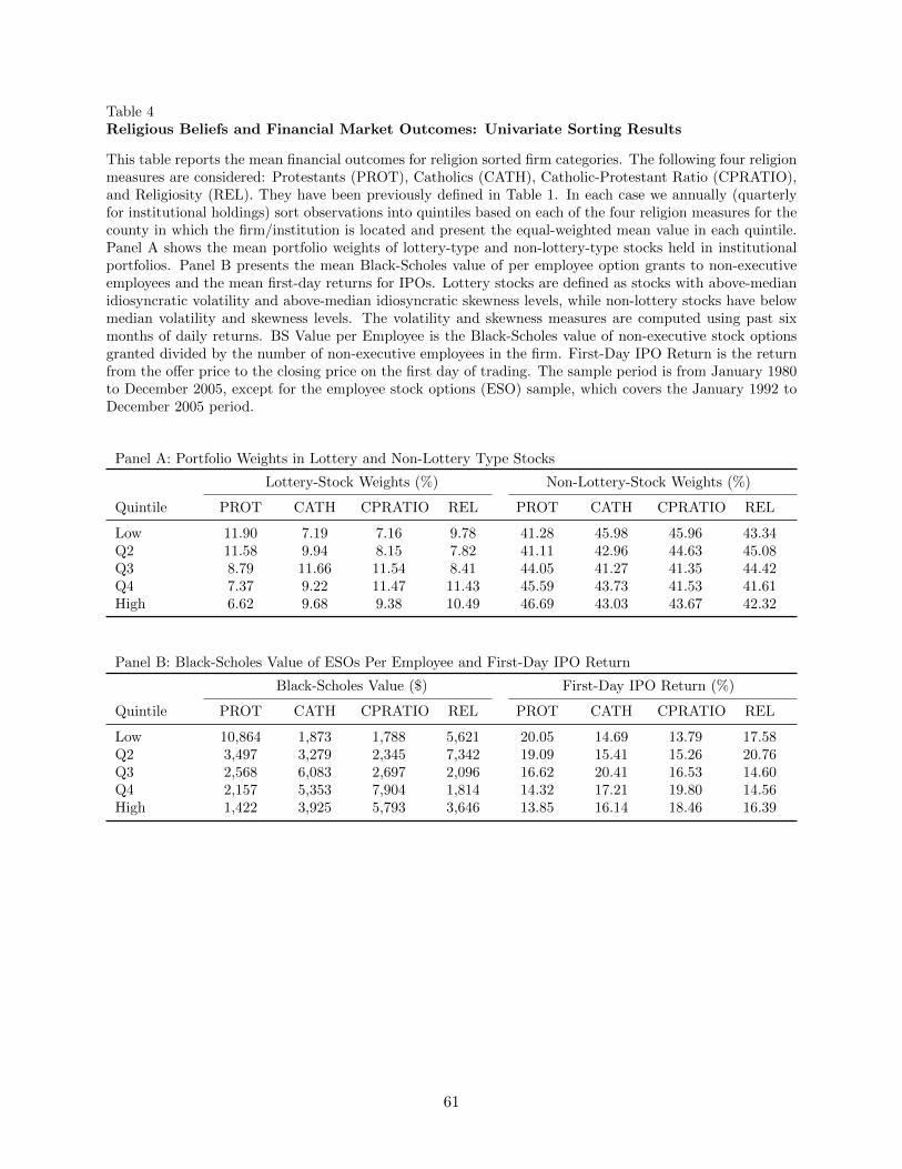
Table 4Religious Beliefs and Financial Market Outcomes: Univariate Sorting Results
This table reports the mean financial outcomes for religion sorted firm categories. The following four religionmeasures are considered: Protestants (PROT), Catholics (CATH), Catholic-Protestant Ratio (CPRATIO),and Religiosity (REL). They have been previously defined in Table 1. In each case we annually (quarterlyfor institutional holdings) sort observations into quintiles based on each of the four religion measures for thecounty in which the firm/institution is located and present the equal-weighted mean value in each quintile.Panel A shows the mean portfolio weights of lottery-type and non-lottery-type stocks held in institutionalportfolios. Panel B presents the mean Black-Scholes value of per employee option grants to non-executiveemployees and the mean first-day returns for IPOs. Lottery stocks are defined as stocks with above-medianidiosyncratic volatility and above-median idiosyncratic skewness levels, while non-lottery stocks have belowmedian volatility and skewness levels. The volatility and skewness measures are computed using past sixmonths of daily returns. BS Value per Employee is the Black-Scholes value of non-executive stock optionsgranted divided by the number of non-executive employees in the firm. First-Day IPO Return is the returnfrom the offer price to the closing price on the first day of trading. The sample period is from January 1980to December 2005, except for the employee stock options (ESO) sample, which covers the January 1992 toDecember 2005 period.
Panel A: Portfolio Weights in Lottery and Non-Lottery Type Stocks
Lottery-Stock Weights (%) Non-Lottery-Stock Weights (%)
Quintile PROT CATH CPRATIO REL PROT CATH CPRATIO REL
Low 11.90 7.19 7.16 9.78 41.28 45.98 45.96 43.34Q2 11.58 9.94 8.15 7.82 41.11 42.96 44.63 45.08Q3 8.79 11.66 11.54 8.41 44.05 41.27 41.35 44.42Q4 7.37 9.22 11.47 11.43 45.59 43.73 41.53 41.61High 6.62 9.68 9.38 10.49 46.69 43.03 43.67 42.32
Panel B: Black-Scholes Value of ESOs Per Employee and First-Day IPO Return
Black-Scholes Value ($) First-Day IPO Return (%)
Quintile PROT CATH CPRATIO REL PROT CATH CPRATIO REL
Low 10,864 1,873 1,788 5,621 20.05 14.69 13.79 17.58Q2 3,497 3,279 2,345 7,342 19.09 15.41 15.26 20.76Q3 2,568 6,083 2,697 2,096 16.62 20.41 16.53 14.60Q4 2,157 5,353 7,904 1,814 14.32 17.21 19.80 14.56High 1,422 3,925 5,793 3,646 13.85 16.14 18.46 16.39
61

Table 5Institutional Portfolio Weight Regression Estimates
This table presents estimates from OLS regressions of institutional lottery-stock, non-lottery-stock, and
recent initial public offering (IPO) holdings on religion measures for the county in which the institution is
located and other control variables. Panel A presents results for the baseline sample that excludes very
large institutions in counties (see Table 2, Panel B). The dependent variable in specifications (1) to (4)
is the proportion of the institution’s portfolio held in lottery-type stocks, while the dependent variable in
specifications (5) to (8) is the portfolio weight in non-lottery-type stocks. In Panel B, the dependent variable
is either the weight in all recent IPOs (specifications (1) to (4)) or non-local IPOs (specifications (5) to (8)).
Recent IPOs refer to firms that went public in the last one quarter. Non-local IPOs are new firms that
are located at least 250 miles away from the institutional location. Panel C presents the estimates for the
subsample of very large institutions only. Panels D and E report the estimates for various other subsamples
of institutions. The dependent variable in Panel D (Panel E) is the portfolio weight in lottery- (non-lottery-)
type stocks. For conciseness, in all panels except Panel A, the control variable estimates are suppressed. In
Panels D and E, each row presents estimates for the religion measures from each of four separate regressions
corresponding to specifications (1) to (4) or specifications (5) to (8) of the respective regressions in Panel
A. The main estimates from Panel A are reprinted as the “Baseline”. Rows (1) to (3) in Panels D and E
show the estimates for alternative definitions of very large institutions. In row (1), large institutions are
defined every quarter as the largest 100 institutions by portfolio size. In row (2), large institutions are
defined every quarter as institutions with portfolio size exceeding the median portfolio size in the quarter.
In row (3), large institutions are those with portfolio size exceeding $1 billion. Concentrated (diversified)
institutions are those above (below) the median portfolio concentration in the quarter. Banks and insurance
companies are considered “Conservative”, while investment companies, independent investment advisors and
others are considered “Aggressive”. Following Bushee (1998), we define quasi-indexers as institutions that
have diversified portfolio holdings and low portfolio turnover. The remaining institutions are labeled as
non-quasi-indexers. In the last two tests, we estimate the lottery weight regressions by pooling data from
the last quarter and the first three quarters of all years, respectively. All regressions in all panels include a
set of dummy variables for each quarter-year combination and institution type. To improve readability, the
coefficient estimates of CPRATIO have been multiplied by 100 in all regressions. All remaining variables
have been previously defined in Table 1. The sample period is from January 1980 to December 2005. Robust
t-statistics, clustered by county, are reported below the coefficient estimates (Panels A, B, and C) or to the
right of the coefficient estimates (Panels D and E).
62

Table 5 – Continued from previous page
Institutional Portfolio Weight Regression Estimates
Panel A: Baseline EstimatesDependent variable: Quarter-t weight in lottery or non-lottery type stocks in institutional portfolio i.
Lottery Weight Non-Lottery Weight
Variable (1) (2) (3) (4) (5) (6) (7) (8)
PROT −0.041 0.047(−1.58) (1.75)
CATH 0.035 −0.043(2.10) (−2.44)
CPRATIO 0.424 −0.457(2.47) (−2.62)
REL 0.040 −0.049(2.28) (−2.70)
Portfolio Size −8.109 −8.031 −7.958 −7.943 7.919 7.831 7.750 7.724(−2.15) (−2.13) (−2.11) (−2.10) (2.20) (2.18) (2.16) (2.13)
Portfolio Concentration 0.135 0.136 0.135 0.136 −0.118 −0.119 −0.117 −0.119(7.03) (7.03) (7.00) (7.01) (−5.50) (−5.53) (−5.45) (−5.48)
Total Population 0.000 0.000 0.000 0.001 0.000 0.000 0.000 0.000(0.20) (0.10) (−0.03) (0.47) (−0.05) (0.11) (0.15) (−0.28)
Education 0.002 0.001 0.001 0.001 −0.001 −0.001 −0.001 −0.001(4.66) (4.51) (4.22) (4.30) (−4.58) (−4.44) (−4.17) (−4.15)
Male-Female Ratio 0.175 0.227 0.229 0.264 −0.164 −0.226 −0.223 −0.273(2.72) (3.38) (3.66) (3.93) (−2.55) (−3.30) (−3.49) (−3.95)
Married 0.024 0.012 0.020 0.005 −0.036 −0.023 −0.031 −0.014(0.51) (0.29) (0.46) (0.12) (−0.79) (−0.55) (−0.73) (−0.34)
Minority 0.058 0.064 0.060 0.057 −0.063 −0.069 −0.064 −0.062(1.64) (1.78) (1.72) (1.65) (−1.76) (−1.94) (−1.84) (−1.77)
Age 0.002 0.003 0.003 0.003 −0.002 −0.003 −0.003 −0.003(2.84) (2.91) (3.15) (3.45) (−3.21) (−3.14) (−3.43) (−3.72)
Urban 0.021 0.020 0.021 0.028 −0.022 −0.021 −0.024 −0.030(1.32) (1.41) (1.52) (2.10) (−1.36) (−1.39) (−1.60) (−2.19)
Quarter Dummies Yes Yes Yes Yes Yes Yes Yes YesInstitution Type Dummies Yes Yes Yes Yes Yes Yes Yes YesAdjusted R2 0.141 0.141 0.143 0.141 0.156 0.156 0.158 0.156Number of Quarter-Insti Obs 101, 377 101, 377 101, 377 101, 377 101, 377 101, 377 101, 377 101, 377
63

Table 5 – Continued from previous pageInstitutional Portfolio Weight Regression Estimates
Panel B: Institutional Regression Estimates with IPO WeightsDependent variable: Quarter-t weight allocated to recent IPOs in institutional portfolio i.
All IPOs Non-Local IPOs
Variable (1) (2) (3) (4) (5) (6) (7) (8)
PROT −0.368 −0.144(−2.35) (−1.45)
CATH 0.393 0.171(3.55) (2.35)
CPRATIO 2.844 1.317(3.13) (2.47)
REL 0.212 0.122(1.93) (1.75)
(Coefficient estimates of control variables have been suppressed.)
Quarter Dummies Yes Yes Yes Yes Yes Yes Yes YesInstitution Type Dummies Yes Yes Yes Yes Yes Yes Yes YesAdjusted R2 0.016 0.016 0.016 0.015 0.010 0.010 0.010 0.010Number of Quarter-Insti Obs 101, 368 101, 368 101, 368 101, 368 101, 368 101, 368 101, 368 101, 368
Panel C: Sub-Sample Estimates for Very Large InstitutionsDependent variable: Quarter-t weight in lottery or non-lottery type stocks in institutional portfolio i.
Lottery Weight Non-Lottery Weight
Variable (1) (2) (3) (4) (5) (6) (7) (8)
PROT −0.008 0.004(−0.67) (0.20)
CATH 0.008 −0.010(0.76) (−0.76)
CPRATIO 0.044 −0.025(0.54) (−0.25)
REL −0.000 −0.007(−0.02) (−0.47)
(Coefficient estimates of control variables have been suppressed.)
Control Variables Yes Yes Yes Yes Yes Yes Yes YesQuarter Dummies Yes Yes Yes Yes Yes Yes Yes YesInstitution Type Dummies Yes Yes Yes Yes Yes Yes Yes YesAdjusted R2 0.268 0.268 0.268 0.268 0.259 0.259 0.259 0.259Number of Quarter-Inst. Obs 19,601 19,601 19,601 19,601 19,601 19,601 19,601 19,601
64
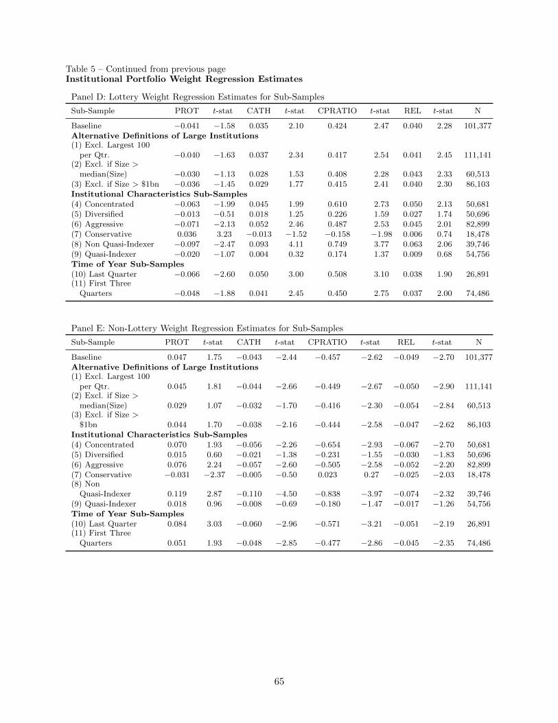
Table 5 – Continued from previous pageInstitutional Portfolio Weight Regression Estimates
Panel D: Lottery Weight Regression Estimates for Sub-Samples
Sub-Sample PROT t-stat CATH t-stat CPRATIO t-stat REL t-stat N
Baseline −0.041 −1.58 0.035 2.10 0.424 2.47 0.040 2.28 101,377Alternative Definitions of Large Institutions(1) Excl. Largest 100
per Qtr. −0.040 −1.63 0.037 2.34 0.417 2.54 0.041 2.45 111,141(2) Excl. if Size >
median(Size) −0.030 −1.13 0.028 1.53 0.408 2.28 0.043 2.33 60,513(3) Excl. if Size > $1bn −0.036 −1.45 0.029 1.77 0.415 2.41 0.040 2.30 86,103Institutional Characteristics Sub-Samples(4) Concentrated −0.063 −1.99 0.045 1.99 0.610 2.73 0.050 2.13 50,681(5) Diversified −0.013 −0.51 0.018 1.25 0.226 1.59 0.027 1.74 50,696(6) Aggressive −0.071 −2.13 0.052 2.46 0.487 2.53 0.045 2.01 82,899(7) Conservative 0.036 3.23 −0.013 −1.52 −0.158 −1.98 0.006 0.74 18,478(8) Non Quasi-Indexer −0.097 −2.47 0.093 4.11 0.749 3.77 0.063 2.06 39,746(9) Quasi-Indexer −0.020 −1.07 0.004 0.32 0.174 1.37 0.009 0.68 54,756Time of Year Sub-Samples(10) Last Quarter −0.066 −2.60 0.050 3.00 0.508 3.10 0.038 1.90 26,891(11) First Three
Quarters −0.048 −1.88 0.041 2.45 0.450 2.75 0.037 2.00 74,486
Panel E: Non-Lottery Weight Regression Estimates for Sub-Samples
Sub-Sample PROT t-stat CATH t-stat CPRATIO t-stat REL t-stat N
Baseline 0.047 1.75 −0.043 −2.44 −0.457 −2.62 −0.049 −2.70 101,377Alternative Definitions of Large Institutions(1) Excl. Largest 100
per Qtr. 0.045 1.81 −0.044 −2.66 −0.449 −2.67 −0.050 −2.90 111,141(2) Excl. if Size >
median(Size) 0.029 1.07 −0.032 −1.70 −0.416 −2.30 −0.054 −2.84 60,513(3) Excl. if Size >
$1bn 0.044 1.70 −0.038 −2.16 −0.444 −2.58 −0.047 −2.62 86,103Institutional Characteristics Sub-Samples(4) Concentrated 0.070 1.93 −0.056 −2.26 −0.654 −2.93 −0.067 −2.70 50,681(5) Diversified 0.015 0.60 −0.021 −1.38 −0.231 −1.55 −0.030 −1.83 50,696(6) Aggressive 0.076 2.24 −0.057 −2.60 −0.505 −2.58 −0.052 −2.20 82,899(7) Conservative −0.031 −2.37 −0.005 −0.50 0.023 0.27 −0.025 −2.03 18,478(8) Non
Quasi-Indexer 0.119 2.87 −0.110 −4.50 −0.838 −3.97 −0.074 −2.32 39,746(9) Quasi-Indexer 0.018 0.96 −0.008 −0.69 −0.180 −1.47 −0.017 −1.26 54,756Time of Year Sub-Samples(10) Last Quarter 0.084 3.03 −0.060 −2.96 −0.571 −3.21 −0.051 −2.19 26,891(11) First Three
Quarters 0.051 1.93 −0.048 −2.85 −0.477 −2.86 −0.045 −2.35 74,486
65

Table 6Robustness Checks: Institutional Portfolio Weight Regression Estimates
This table presents institutional regression estimates using alternative specifications. For conciseness we
report only the estimates of CPRATIO and suppress coefficients of all other variables. The main estimates
from Table 5, Panel A (columns (3) and (7)) are reprinted as “baseline”. In test (1) we control for county-level
religiosity. Next, we control for industry concentration, which is defined as the Herfindahl index of the 48
Fama and French (1997) industry weights in the institution’s portfolio. The two-stage least squares (2SLS)
estimate uses three-year lagged value of the religions variables as an instrument for the concurrent value.
The alternative lottery stock definition classifies lottery stocks as those with below median price in addition
to above median volatility and skewness. In test (5), we estimate the lottery weight regression without
institution type dummies. In test (6), CPDIFF is the difference between the proportions of Catholics and
Protestants in a county. The “Include Mormons and Jews” test uses an alternative measure of CPRATIO,
where the Catholic population includes the Jewish adherents and the Protestant population includes the
Mormons. In test (8), we use lottery sales as the main independent variable instead of CPRATIO, where
lottery sales is defined as the inflation-adjusted per-capita state-level lottery sales. In test (9), both the
state-level lottery sales and CPRATIO are included in our regression. In tests (10) to (12), we estimate the
return regressions for different sub-periods and in tests (13) to (18), we consider several geography based
sub-samples. “Conservatives” in test (11) include banks and insurance companies (institution types 1 and 2).
We control for political environment using a dummy variable that is set to one for states that voted in favor of
the Republican party in the last Presidential elections. The Social Capital variable is a composite index of 14
different state-level measures of community participation and the Trust variable is based on a question in the
General Social Survey that measures the percentage of survey respondents in the state who agrees with the
statement that “Most people can be trusted.” In test (24) we include the average beta (48 monthly returns)
of stocks in an institutional portfolio as an additional regressor. In Panels B and C, we present estimates
from OLS regressions of institutional (non-)lottery-stock weights using state and county fixed effects. In the
first set, we re-estimate the regressions in Table 5, Panel A with state fixed effects and include an interaction
variable between one of the institutional attributes and CATH, PROT, CPRATIO, or REL. In the second
set, we re-estimate the regressions in Table 5, Panel A with the interaction term and county fixed effects
and, therefore, exclude all county-level independent variables. We consider three institutional attributes:
(i) Portfolio Concentration, as defined in Table 1; (ii) “Aggressive” institutions, which includes investment
companies (type 3), independent investment advisors (type 4), and “Others” (type 5); and (iii) Non-Quasi-
Indexer institutions, which have non-diversified portfolios and have high portfolio turnover (Bushee, 1998).
For brevity, we report only the coefficient estimates of the institutional attribute-religion interaction terms.
Panel D presents results with different controls for large counties. In tests (1) to (4) we re-estimate our
baseline regressions with an additional dummy variable that is set to one if the institution is located in one
of the top 5, 10, or 15 counties. The financial center dummy is set to one for institutions located in a county
within the New York, Boston, Chicago, Los Angeles, or San Francisco metropolitan regions. For brevity,
we only report the coefficients estimates of CPRATIO and the dummy variable. Rows (5) to (7) show the
estimates when we exclude New York, exclude the largest counties, or only include institutions in the five
largest counties. In the last three specifications, we re-estimate regressions that include county-level fixed
effects as in Panels B and C but we exclude institutions in the five largest counties. All other variables in the
table have been previously defined in Table 1. To improve readability, the coefficient estimates of CPRATIO
have been multiplied by 100 in all regressions. The sample period is from January 1980 to December 2005.
Robust t-statistics, clustered by county, are reported to the right of or below the coefficient estimates.
66
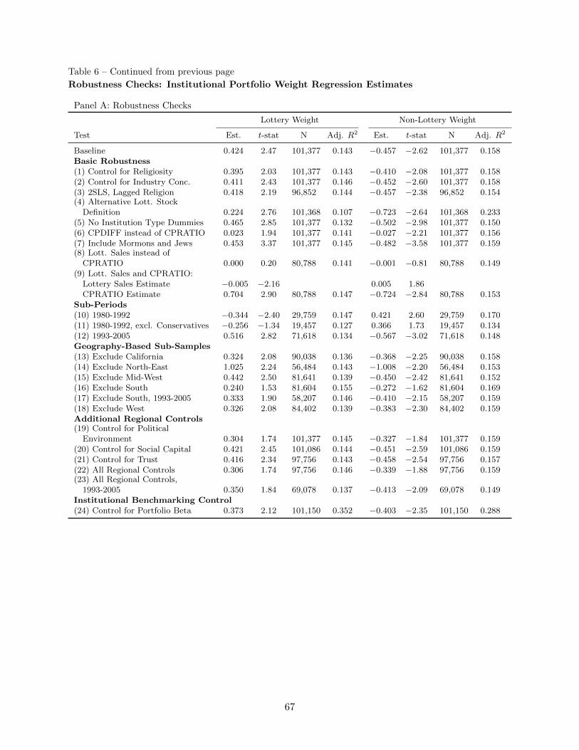
Table 6 – Continued from previous page
Robustness Checks: Institutional Portfolio Weight Regression Estimates
Panel A: Robustness Checks
Lottery Weight Non-Lottery Weight
Test Est. t-stat N Adj. R2 Est. t-stat N Adj. R2
Baseline 0.424 2.47 101,377 0.143 −0.457 −2.62 101,377 0.158Basic Robustness(1) Control for Religiosity 0.395 2.03 101,377 0.143 −0.410 −2.08 101,377 0.158(2) Control for Industry Conc. 0.411 2.43 101,377 0.146 −0.452 −2.60 101,377 0.158(3) 2SLS, Lagged Religion 0.418 2.19 96,852 0.144 −0.457 −2.38 96,852 0.154(4) Alternative Lott. Stock
Definition 0.224 2.76 101,368 0.107 −0.723 −2.64 101,368 0.233(5) No Institution Type Dummies 0.465 2.85 101,377 0.132 −0.502 −2.98 101,377 0.150(6) CPDIFF instead of CPRATIO 0.023 1.94 101,377 0.141 −0.027 −2.21 101,377 0.156(7) Include Mormons and Jews 0.453 3.37 101,377 0.145 −0.482 −3.58 101,377 0.159(8) Lott. Sales instead of
CPRATIO 0.000 0.20 80,788 0.141 −0.001 −0.81 80,788 0.149(9) Lott. Sales and CPRATIO:
Lottery Sales Estimate −0.005 −2.16 0.005 1.86CPRATIO Estimate 0.704 2.90 80,788 0.147 −0.724 −2.84 80,788 0.153
Sub-Periods(10) 1980-1992 −0.344 −2.40 29,759 0.147 0.421 2.60 29,759 0.170(11) 1980-1992, excl. Conservatives −0.256 −1.34 19,457 0.127 0.366 1.73 19,457 0.134(12) 1993-2005 0.516 2.82 71,618 0.134 −0.567 −3.02 71,618 0.148Geography-Based Sub-Samples(13) Exclude California 0.324 2.08 90,038 0.136 −0.368 −2.25 90,038 0.158(14) Exclude North-East 1.025 2.24 56,484 0.143 −1.008 −2.20 56,484 0.153(15) Exclude Mid-West 0.442 2.50 81,641 0.139 −0.450 −2.42 81,641 0.152(16) Exclude South 0.240 1.53 81,604 0.155 −0.272 −1.62 81,604 0.169(17) Exclude South, 1993-2005 0.333 1.90 58,207 0.146 −0.410 −2.15 58,207 0.159(18) Exclude West 0.326 2.08 84,402 0.139 −0.383 −2.30 84,402 0.159Additional Regional Controls(19) Control for Political
Environment 0.304 1.74 101,377 0.145 −0.327 −1.84 101,377 0.159(20) Control for Social Capital 0.421 2.45 101,086 0.144 −0.451 −2.59 101,086 0.159(21) Control for Trust 0.416 2.34 97,756 0.143 −0.458 −2.54 97,756 0.157(22) All Regional Controls 0.306 1.74 97,756 0.146 −0.339 −1.88 97,756 0.159(23) All Regional Controls,
1993-2005 0.350 1.84 69,078 0.137 −0.413 −2.09 69,078 0.149Institutional Benchmarking Control(24) Control for Portfolio Beta 0.373 2.12 101,150 0.352 −0.403 −2.35 101,150 0.288
67
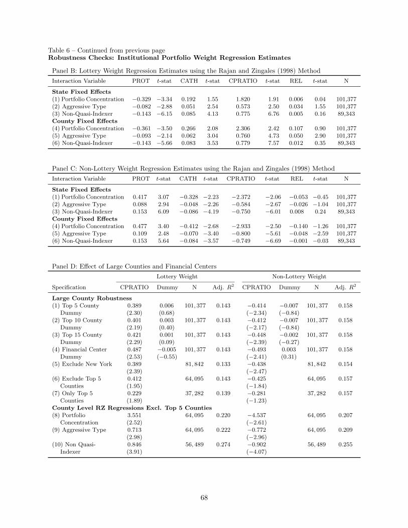
Table 6 – Continued from previous pageRobustness Checks: Institutional Portfolio Weight Regression Estimates
Panel B: Lottery Weight Regression Estimates using the Rajan and Zingales (1998) Method
Interaction Variable PROT t-stat CATH t-stat CPRATIO t-stat REL t-stat N
State Fixed Effects(1) Portfolio Concentration −0.329 −3.34 0.192 1.55 1.820 1.91 0.006 0.04 101,377(2) Aggressive Type −0.082 −2.88 0.051 2.54 0.573 2.50 0.034 1.55 101,377(3) Non-Quasi-Indexer −0.143 −6.15 0.085 4.13 0.775 6.76 0.005 0.16 89,343County Fixed Effects(4) Portfolio Concentration −0.361 −3.50 0.266 2.08 2.306 2.42 0.107 0.90 101,377(5) Aggressive Type −0.093 −2.14 0.062 3.04 0.760 4.73 0.050 2.90 101,377(6) Non-Quasi-Indexer −0.143 −5.66 0.083 3.53 0.779 7.57 0.012 0.35 89,343
Panel C: Non-Lottery Weight Regression Estimates using the Rajan and Zingales (1998) Method
Interaction Variable PROT t-stat CATH t-stat CPRATIO t-stat REL t-stat N
State Fixed Effects(1) Portfolio Concentration 0.417 3.07 −0.328 −2.23 −2.372 −2.06 −0.053 −0.45 101,377(2) Aggressive Type 0.088 2.94 −0.048 −2.26 −0.584 −2.67 −0.026 −1.04 101,377(3) Non-Quasi-Indexer 0.153 6.09 −0.086 −4.19 −0.750 −6.01 0.008 0.24 89,343County Fixed Effects(4) Portfolio Concentration 0.477 3.40 −0.412 −2.68 −2.933 −2.50 −0.140 −1.26 101,377(5) Aggressive Type 0.109 2.48 −0.070 −3.40 −0.800 −5.61 −0.048 −2.59 101,377(6) Non-Quasi-Indexer 0.153 5.64 −0.084 −3.57 −0.749 −6.69 −0.001 −0.03 89,343
Panel D: Effect of Large Counties and Financial Centers
Lottery Weight Non-Lottery Weight
Specification CPRATIO Dummy N Adj. R2 CPRATIO Dummy N Adj. R2
Large County Robustness(1) Top 5 County 0.389 0.006 101, 377 0.143 −0.414 −0.007 101, 377 0.158
Dummy (2.30) (0.68) (−2.34) (−0.84)(2) Top 10 County 0.401 0.003 101, 377 0.143 −0.412 −0.007 101, 377 0.158
Dummy (2.19) (0.40) (−2.17) (−0.84)(3) Top 15 County 0.421 0.001 101, 377 0.143 −0.448 −0.002 101, 377 0.158
Dummy (2.29) (0.09) (−2.39) (−0.27)(4) Financial Center 0.487 −0.005 101, 377 0.143 −0.493 0.003 101, 377 0.158
Dummy (2.53) (−0.55) (−2.41) (0.31)(5) Exclude New York 0.389 81, 842 0.133 −0.438 81, 842 0.154
(2.39) (−2.47)(6) Exclude Top 5 0.412 64, 095 0.143 −0.425 64, 095 0.157
Counties (1.95) (−1.84)(7) Only Top 5 0.229 37, 282 0.139 −0.281 37, 282 0.157
Counties (1.89) (−1.23)County Level RZ Regressions Excl. Top 5 Counties(8) Portfolio 3.551 64, 095 0.220 −4.537 64, 095 0.207
Concentration (2.52) (−2.61)(9) Aggressive Type 0.713 64, 095 0.222 −0.772 64, 095 0.209
(2.98) (−2.96)(10) Non Quasi- 0.846 56, 489 0.274 −0.902 56, 489 0.255
Indexer (3.91) (−4.07)
68
Table 7Employee Stock Option Regression Estimates
This table reports marginal effects computed at the mean from Tobit regressions of employee stock option
grants on religion measures for the county in which the institution is located and other control variables.
Stock option grants are measured as the natural logarithm of the Black-Scholes value of per-employee option
grants to non-executive employees. All independent variables have been previously defined in Table 1. Panel
A shows the full sample estimates for baseline specifications, Panel B presents results from extended speci-
fications with neighborhood controls such as local labor market and social interaction variables, and Panel
C reports estimates obtained using alternative specifications and different subsamples. In Panels B and C,
for conciseness, the estimates of all control variables are suppressed. In Panel B, the following neighborhood
controls are considered: (i) tight labor market dummy that is set to one if the MSA unemployment rate is
higher than the average MSA employment rate, (ii) local beta that is the firm’s exposure to the local return
index computed using the Pirinsky and Wang (2006) method, (iii) the state-level non-compete enforceability
index obtained from Garmaise (2010), (iv) the market-adjusted MSA return that is the median 12-month
return of all firms headquartered in the MSA, (v) the industry cluster dummy is set to one for firms that are
located in MSAs with an industry cluster, and (vi) option grants at other firms in the MSA is the average
Black-Scholes value of option grants at other firms in the MSA. In specifications (5) and (6), high and low
CPRATIO subsamples include firms that are located in counties with above and below median CPRATIO
levels, respectively. In Panel C, the main estimates from specifications (5) to (8) in Panel A are reprinted as
the “Baseline”. Each row presents estimates for the religion measures from each of four separate regressions
corresponding to specifications (5) to (8) in Panel A. We first consider an alternative measure of option
grants and use the annual number of granted options per non-executive employee as a dependent variable.
In this regression we also control for the volatility of the firm (based on the past 60 month stock return
reported in ExecuComp), as well as the natural logarithm of the beginning of the year stock price. In the
second regression in this panel, we estimate the ESO regressions using OLS, where we only consider the
subsample of firms that grant employee stock options. The high (low) volatility subsamples consist of firms
with above (below) median volatility. Larger (smaller) firms are defined as those with fiscal year sales greater
(smaller) than the median firm in the sample. The high (low) income subsample consists of firms located in
counties with above (below) median per-capita income (median is based on the sample of firm observations)
per year. High and low education samples are similarly defined per year using the proportion of county
residents above age 25 with bachelor’s degree or higher. Industry dummies are based on 30 Fama-French
industries. The sample period is from January 1992 to December 2005. Robust z-statistics (t-statistics for
OLS regressions), clustered by county, are reported below the coefficient estimates (Panels A and B) or to
the right of the coefficient estimates (Panel C).
69

Table 7 – Continued from previous page
Employee Stock Option Regression Estimates
Panel A: ESO Regression Estimates for the Full SampleDependent variable: Ln(1 + Black-Scholes value of ESOs per employee) in year t.
Variable (1) (2) (3) (4) (5) (6) (7) (8)
PROT −2.232 −1.517(−3.74) (−2.84)
CATH 0.951 0.717(2.75) (1.54)
CPRATIO 0.123 0.107(4.04) (3.16)
REL −0.361 −0.253(−0.52) (−0.48)
Ln(Sales) −0.299 −0.299 −0.298 −0.296 −0.297 −0.297 −0.294 −0.298(−10.36) (−10.07) (−10.14) (−9.77) (−10.20) (−10.14) (−10.06) (−10.13)
Tobin’s Q 0.189 0.194 0.191 0.193 0.178 0.179 0.177 0.179(7.57) (7.43) (7.45) (7.60) (7.94) (7.92) (7.90) (7.93)
R&D Expenses 6.192 6.626 6.346 6.770 5.488 5.659 5.464 5.743(4.95) (5.09) (5.07) (5.01) (4.79) (4.95) (4.90) (4.85)
Total Population 0.016 0.020 0.003 0.049(0.60) (0.71) (0.10) (1.93)
Education 0.022 0.022 0.019 0.026(3.45) (3.33) (3.05) (3.52)
Male-Female Ratio 4.681 5.987 6.276 4.973(2.45) (2.83) (3.10) (2.26)
Married 1.764 1.582 1.438 1.757(2.32) (2.00) (1.91) (2.10)
Minority 0.678 0.839 0.685 0.642(1.13) (1.31) (1.18) (0.98)
Age 0.018 0.033 0.020 0.043(0.68) (1.21) (0.76) (1.61)
Urban 0.437 0.752 0.703 0.971(0.97) (1.67) (1.59) (2.14)
Industry Dummies Yes Yes Yes Yes Yes Yes Yes YesYear Dummies Yes Yes Yes Yes Yes Yes Yes YesPseudo R2 0.091 0.090 0.091 0.089 0.095 0.094 0.095 0.094Number of Firm-Year Obs 14, 557 14, 557 14, 557 14, 557 14, 557 14, 557 14, 557 14, 557
70

Table 7 – Continued from previous page
Employee Stock Option Regression Estimates
Panel B: ESO Regression Estimates With Neighborhood ControlsDependent variable: Ln(1 + Black-Scholes value of ESOs per employee) in year t.
MSA CPRATIO
Low HighVariable (1) (2) (3) (4) (5) (6)
CPRATIO 0.099 0.081(2.82) (2.23)
Tight Labor Market Dummy 0.098 0.091 0.068 0.068 0.224 −0.016(0.91) (0.82) (0.62) (0.60) (1.46) (−0.08)
Local Beta 0.066 0.070 0.069 0.074 0.044 0.104(2.89) (3.10) (3.07) (3.25) (1.35) (1.80)
Non-Compete Enforceability Index −0.079 −0.054 −0.044 −0.030 0.038 −0.032(−2.40) (−1.63) (−1.35) (−0.91) (0.69) (−0.64)
Median Market-Adj. MSA Return −0.038 −0.016 −0.108 −0.102 −0.260 0.050(−0.20) (−0.09) (−0.55) (−0.51) (−0.87) (0.18)
Industry Cluster Dummy 0.131 0.066 0.104 0.062 −0.063 0.232(1.19) (0.62) (1.01) (0.58) (−0.49) (1.06)
Option Grants at Other Firms in MSA 0.071 0.046 −0.006 0.124(1.84) (1.17) (−0.14) (1.79)
(Coefficient estimates of other variables have been suppressed.)
Control Variables Yes Yes Yes Yes Yes YesYear Dummies Yes Yes Yes Yes Yes YesIndustry Dummies Yes Yes Yes Yes Yes YesPseudo R2 0.095 0.096 0.097 0.097 0.070 0.118Number of Firm-Year Obs 12, 666 12, 666 12, 152 12, 152 5, 767 6, 385
Panel C: Estimates From Alternative Specifications and Sub-Samples
Test PROT z-stat CATH z-stat CPRATIO z-stat REL z-stat N
Baseline −1.517 −2.89 0.717 1.55 0.107 3.16 −0.253 −0.48 14, 557Alternative Specifications(1) Dep Var: Num of
Options −1.167 −2.88 0.608 1.73 0.085 3.33 −0.108 −0.27 14, 557(2) Firms with ESO Plan:
OLS −1.022 −2.50 0.191 0.47 0.080 3.12 −0.349 −0.80 8, 499Firm Characteristics Sub-Samples(3) High Volatility Firms −3.119 −4.10 1.501 2.17 0.166 3.26 −0.120 −0.16 7, 291(4) Low Volatility Firms −0.820 −1.62 0.648 1.62 0.075 2.15 0.296 0.55 7, 266(5) Smaller Firms −2.880 −3.84 1.283 2.12 0.157 3.31 −0.258 −0.28 7, 275(6) Larger Firms −0.855 −1.40 0.245 0.48 0.060 1.63 −0.260 −0.49 7, 282Location Characteristics Sub-Samples(7) High Income −3.872 −1.96 2.769 2.15 0.170 2.12 1.263 1.17 7, 533(8) Low Income −0.915 −1.75 0.322 0.65 0.077 1.83 −0.522 −0.79 7, 024(9) High Education −4.203 −4.92 2.879 3.99 0.201 3.79 0.560 0.60 7, 381(10) Low Education −0.645 −1.30 0.180 0.40 0.056 1.59 −0.178 −0.33 7, 176
71
Table 8Robustness Checks: ESO Regression Estimates
This table presents several alternative versions of the employee stock option regressions in Table 7 as robust-
ness checks. Unless otherwise stated, we run Tobit regressions with the natural logarithm of the Black-Scholes
value of options granted to non-executive employees as dependent variable. For conciseness we report only
the marginal effect estimates computed at the mean for CPRATIO. In the first test, we control for county-
level religiosity. Next, we estimate an instrumental variable Tobit specification, where the three-year lagged
value of the religion variables is used as an instrument for the concurrent value. The set of “Additional Con-
trol Variables” includes contemporaneous stock return, past 2-year stock return, industry volatility, earnings
volatility, and measures of cash constraints (cash balances, cash dividends, cash flow and leverage). In test
(5), CPDIFF is the difference of the natural logarithm of Catholics and Protestants in a county. The “In-
clude Mormons and Jews” test uses an alternative measure of CPRATIO, where the Catholic population
includes the Jewish adherents and the Protestant population includes the Mormons. The “Binary dependent
variable” specification reports the results of logit regressions where the dependent variable equals one if the
firm has a broad-based employee stock option plan and zero otherwise. In test (9), we exclude technology
firms, as defined in Table 1. The CEO option grant is the natural logarithm of the Black-Scholes value of the
stock options granted to the CEO in the fiscal year. In tests (11) to (14), we estimate the ESO regressions
for different sub-periods and in tests (15) to (19), we consider several geography based sub-samples. In the
last four tests, we include additional state-level control variables in the specification. We control for political
environment using a dummy variable that is set to one for states that voted in favor of the Republican party
in the last Presidential elections. The Social Capital variable is a composite index of 14 different state-level
measures of community participation and the Trust variable is based on a question in the General Social
Survey that measures the percentage of survey respondents in the state who agrees with the statement that
“Most people can be trusted.” In Panel B, we present ESO regression estimates using specifications that
include state and county fixed effects. In the first set, we re-estimate the regressions in Table 7, Panel A with
state fixed effects and include an interaction variable between the high volatility firm dummy and CATH,
PROT, CPRATIO, or REL. In the second set, we re-estimate the regressions in Table 7, Panel A with the
interaction term and county fixed effects and, therefore, exclude all county-level independent variables. The
high volatility dummy is one if the firm’s stock return volatility is above the median monthly return volatility
(measured over the prior 60 months). In tests (2) and (5), we estimate the state fixed effects regressions
using a sub-sample of small firms, while in tests (3) and (6), we estimate the state fixed effects regressions
using a sub-sample of large firms. Large (small) firms are defined as those with fiscal year sales greater
(smaller) than the median firm in the sample. The state and county fixed effects regressions are estimated
using OLS on the subsample of firms that offer an employee stock option plan. For brevity, we report only
the coefficient estimates of the volatility-religion interaction terms. The sample period is from January 1992
to December 2005. Robust z-statistics (t-statistics for OLS regressions), clustered by county, are reported
to the right of the coefficient estimates.
72

Table 8 – Continued from previous page
Robustness Checks: ESO Regression Estimates
Panel A: Additional Robustness Checks
CPRATIOTest Estimate z-statistic N Pseudo R2
Basic Robustness(1) Control for Religiosity 0.136 3.45 14, 557 0.095(2) IV Tobit, Lagged Religion 0.108 3.24 14, 491 0.420(3) No Industry Dummies 0.141 3.52 14, 557 0.074(4) Additional Control Variables 0.092 2.07 10, 870 0.085(5) Use CPDIFF instead of C/P 0.090 2.56 14, 557 0.094(6) Include Mormons and Jews 0.076 2.69 14, 491 0.094(7) Binary Dependent Variable 0.012 1.95 14, 557 0.209(8) Binary Dep Var w/o Industry Dummies 0.015 2.25 14, 557 0.176(9) Exclude Technology Firms 0.096 3.11 12, 248 0.068(10) Control for CEO Option Grant 0.099 3.00 14, 555 0.098Sub-Periods(11) 1993 Cross-Section Only 0.171 2.89 875 0.108(12) 2000 Cross-Section Only 0.166 3.08 1, 115 0.094(13) 1992-2000 0.093 2.22 9, 159 0.099(14) 2001-2005 0.123 2.63 5, 398 0.087Geography-Based Sub-Samples(15) Exclude California 0.062 2.20 12, 092 0.075(16) Exclude Northeast 0.144 1.69 11, 049 0.096(17) Exclude Midwest 0.106 2.48 11, 073 0.102(18) Exclude South 0.095 1.98 10, 580 0.109(19) Exclude West 0.069 2.38 10, 969 0.072Additional Regional Controls(20) Control for Political Environment 0.101 2.87 14,557 0.095(21) Control for Social Capital 0.105 3.13 14,523 0.095(22) Control for Trust 0.106 3.06 14,168 0.095(23) Include All Regional Controls 0.101 2.74 14,168 0.096
Panel B: ESO Regression Estimates using the Rajan and Zingales (1998) Method
Interaction Variable PROT t-stat CATH t-stat CPRATIO t-stat REL t-stat N
State Fixed Effects(1) High Volatility Firm −1.004 −2.50 0.747 2.29 0.054 2.25 0.072 0.16 8,499(2) High Volatility (Small
Firms) −1.544 −2.50 0.897 1.77 0.071 2.06 −0.056 −0.61 4,253(3) High Volatility (Large
Firms) −1.012 −2.13 0.493 1.16 0.055 1.90 −0.048 −0.25 4,246County Fixed Effects(4) High Volatility Firm −0.770 −1.63 0.837 2.20 0.045 1.49 0.493 1.03 8,499(5) High Volatility (Small
Firms) −1.948 −2.81 1.646 3.04 0.103 2.67 0.380 0.63 4,253(6) High Volatility (Large
Firms) −0.642 −1.22 0.397 0.74 0.033 0.89 0.127 0.19 4,246
73
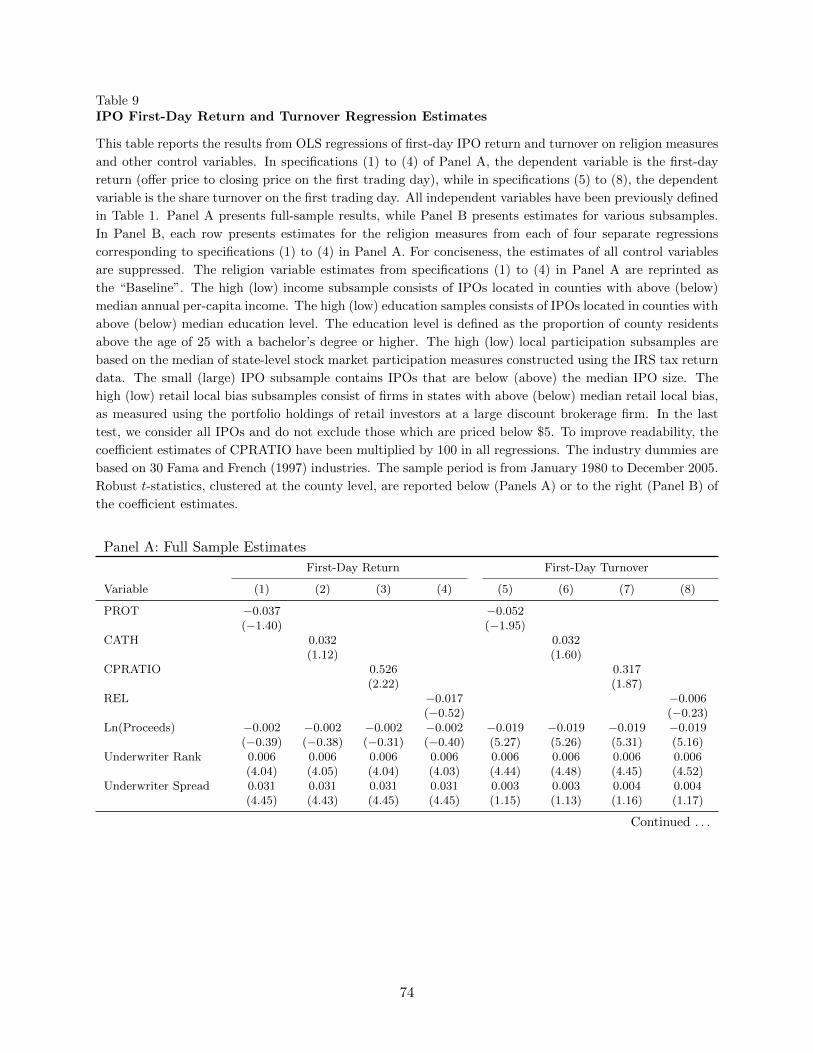
Table 9IPO First-Day Return and Turnover Regression Estimates
This table reports the results from OLS regressions of first-day IPO return and turnover on religion measures
and other control variables. In specifications (1) to (4) of Panel A, the dependent variable is the first-day
return (offer price to closing price on the first trading day), while in specifications (5) to (8), the dependent
variable is the share turnover on the first trading day. All independent variables have been previously defined
in Table 1. Panel A presents full-sample results, while Panel B presents estimates for various subsamples.
In Panel B, each row presents estimates for the religion measures from each of four separate regressions
corresponding to specifications (1) to (4) in Panel A. For conciseness, the estimates of all control variables
are suppressed. The religion variable estimates from specifications (1) to (4) in Panel A are reprinted as
the “Baseline”. The high (low) income subsample consists of IPOs located in counties with above (below)
median annual per-capita income. The high (low) education samples consists of IPOs located in counties with
above (below) median education level. The education level is defined as the proportion of county residents
above the age of 25 with a bachelor’s degree or higher. The high (low) local participation subsamples are
based on the median of state-level stock market participation measures constructed using the IRS tax return
data. The small (large) IPO subsample contains IPOs that are below (above) the median IPO size. The
high (low) retail local bias subsamples consist of firms in states with above (below) median retail local bias,
as measured using the portfolio holdings of retail investors at a large discount brokerage firm. In the last
test, we consider all IPOs and do not exclude those which are priced below $5. To improve readability, the
coefficient estimates of CPRATIO have been multiplied by 100 in all regressions. The industry dummies are
based on 30 Fama and French (1997) industries. The sample period is from January 1980 to December 2005.
Robust t-statistics, clustered at the county level, are reported below (Panels A) or to the right (Panel B) of
the coefficient estimates.
Panel A: Full Sample Estimates
First-Day Return First-Day Turnover
Variable (1) (2) (3) (4) (5) (6) (7) (8)
PROT −0.037 −0.052(−1.40) (−1.95)
CATH 0.032 0.032(1.12) (1.60)
CPRATIO 0.526 0.317(2.22) (1.87)
REL −0.017 −0.006(−0.52) (−0.23)
Ln(Proceeds) −0.002 −0.002 −0.002 −0.002 −0.019 −0.019 −0.019 −0.019(−0.39) (−0.38) (−0.31) (−0.40) (5.27) (5.26) (5.31) (5.16)
Underwriter Rank 0.006 0.006 0.006 0.006 0.006 0.006 0.006 0.006(4.04) (4.05) (4.04) (4.03) (4.44) (4.48) (4.45) (4.52)
Underwriter Spread 0.031 0.031 0.031 0.031 0.003 0.003 0.004 0.004(4.45) (4.43) (4.45) (4.45) (1.15) (1.13) (1.16) (1.17)
Continued . . .
74

Table 9 – Continued from previous page
IPO First-Day Return and Turnover Regression Estimates
Panel A: Full Sample Estimates (Continued)
First-Day Return First-Day Turnover
Variable (1) (2) (3) (4) (5) (6) (7) (8)
Offer Price Revision 0.551 0.551 0.550 0.551 0.183 0.183 0.183 0.184(13.06) (13.08) (13.07) (13.07) (7.85) (7.83) (7.85) (7.85)
Pre-IPO Market Return 11.562 11.554 11.501 11.601 1.758 1.774 1.751 1.813(7.48) (7.53) (7.47) (7.55) (1.33) (1.35) (1.33) (1.39)
Ln(1 + Firm Age) −0.010 −0.011 −0.011 −0.010 0.005 0.005 0.005 0.005(−3.60) (−3.65) (−3.67) (−3.58) (2.28) (2.25) (2.28) (2.34)
Technology Firm Dummy 0.042 0.042 0.041 0.042 −0.014 −0.014 −0.014 −0.013(3.93) (3.92) (3.89) (3.92) (−1.54) (−1.52) (−1.58) (−1.47)
Total Population −0.001 −0.001 −0.002 −0.001 −0.001 0.002 −0.002 0.000(−0.28) (−0.39) (−0.76) (0.27) (−1.00) (−1.00) (−1.01) (−0.25)
Education 0.046 0.043 0.035 0.059 0.002 0.002 0.001 0.014(0.94) (0.91) (0.77) (1.17) (0.05) (0.05) (0.02) (0.39)
Male-Female Ratio 0.193 0.254 0.256 0.187 −0.163 −0.090 −0.100 −0.133(1.93) (2.24) (2.51) (1.39) (−2.31) (−1.35) (−1.53) (−1.61)
Married 0.012 0.005 −0.003 0.011 −0.005 −0.013 −0.016 0.008(0.15) (0.06) (−0.03) (0.14) (−0.12) (−0.35) (−0.42) (−0.21)
Minority 0.088 0.093 0.090 0.082 0.018 0.021 0.016 0.012(1.44) (1.46) (1.55) (1.30) (0.59) (0.70) (0.54) (0.38)
Age 0.003 0.003 0.003 0.003 −0.001 −0.001 −0.001 −0.001(1.65) (1.75) (1.60) (1.77) (−1.04) (−0.64) (−0.75) (−0.41)
Urban −0.023 −0.019 −0.024 −0.014 −0.023 −0.021 −0.021 −0.015(−0.97) (−0.82) (−1.02) (−0.62) (−1.55) (−1.19) (−1.21) (−0.84)
Year Dummies Yes Yes Yes Yes Yes Yes Yes YesIndustry Dummies Yes Yes Yes Yes Yes Yes Yes YesAdjusted R2 0.388 0.388 0.389 0.388 0.244 0.243 0.244 0.243Number of IPOs 6,254 6,254 6,254 6,254 6,100 6,100 6,100 6,100
75

Table 9 – Continued from previous page
IPO First-Day Return and Turnover Regression Estimates
Panel B: Return Regression Estimates For Market Participation and Local Bias Sub-Samples
Sub-Sample PROT t-stat CATH t-stat CPRATIO t-stat REL t-stat N
Baseline −0.037 −1.40 0.032 1.12 0.526 2.22 −0.017 −0.52 6,254Market Participation Proxy(1) High Income −0.116 −1.86 0.101 1.78 0.927 2.60 0.036 0.53 3,149(2) High Income,
1993-2005 −0.145 −2.19 0.115 1.93 1.092 2.92 0.033 0.47 2,760(3) Low Income −0.014 −0.56 −0.013 −0.57 −0.038 −0.17 −0.045 −1.88 3,105(4) High Education −0.043 −0.74 0.081 1.41 0.803 2.15 0.048 0.73 3,154(5) High Education,
1993-2005 −0.103 −1.47 0.104 1.44 1.100 2.62 0.042 0.53 2,297(6) Low Education −0.022 −0.86 −0.013 −0.59 0.080 0.34 −0.072 −3.02 3,100(7) High Part States,
1998-2005 −0.570 −2.87 0.184 1.25 1.350 1.90 −0.026 −0.15 718(8) Low Part States,
1998-2005 0.036 0.26 −0.062 −0.45 0.544 0.43 −0.163 −1.19 719IPO Characteristics and Retail Clientele(9) Price Below Median −0.063 −2.04 0.055 2.21 0.504 2.14 −0.001 −0.00 3,374(10) Price Above Median 0.041 0.12 0.010 0.27 0.418 1.44 −0.016 −0.40 3,279(11) Small IPOs −0.060 −1.58 0.072 2.27 0.724 2.40 0.017 0.44 3,112(12) Large IPOs −0.010 −0.33 −0.019 −0.50 0.286 0.94 −0.050 −1.22 3,142(13) High First-Day
Turnover −0.073 −1.78 0.054 1.28 0.817 2.50 −0.021 −0.43 3,265(14) Low First-Day
Turnover 0.020 0.68 −0.001 −0.43 −0.025 −0.12 −0.014 −0.52 2,989(15) High Retail Local
Bias −0.006 −0.12 0.071 1.66 1.029 2.45 0.052 0.80 2,746(16) Low Retail Local Bias 0.014 0.37 −0.013 −0.47 0.105 0.38 −0.031 −0.98 3,508Local Bias and Income(17) Low Income, Low LB 0.016 0.41 −0.055 −1.84 −0.335 −0.99 −0.060 −1.60 1,753(18) Low Income, High LB −0.042 −1.21 0.051 1.49 0.408 1.39 −0.025 −0.75 1,352(19) High Income, Low LB −0.074 −0.97 0.058 0.99 0.478 1.23 0.022 0.35 1,755(20) High Income, High
LB 0.069 0.41 0.121 1.04 2.130 2.17 0.128 0.91 1,394Other Tests(21) No Min $5 Price
Filter −0.043 −1.73 0.035 1.34 0.540 2.55 −0.016 −0.53 6,653
76

Table 10Robustness Checks: IPO First-Day Return Regression Estimates
This table reports several alternative versions of the IPO return regressions as robustness checks. In Panel
A, we re-estimate the regressions in Table 9, Panel A and, for conciseness, we only report the CPRATIO
coefficient estimates. In the first test, we control for the overall level of religiosity in the county. The two-
stage least squares (2SLS) estimate uses three-year lagged value of the religion variables as an instrument
for the concurrent value. In test (3), we do not include industry dummies in the specification. In test (4)
the main independent variable is CPDIFF, which is the difference between the proportions of Catholics and
Protestants in a county. The “Include Mormons and Jews” test uses an alternative measure of CPRATIO,
where the Catholic population includes the Jewish adherents and the Protestant population includes the
Mormons. In test (6), we use lottery sales as the main independent variable instead of CPRATIO, where
lottery sales is defined as the inflation-adjusted per-capita state-level lottery sales. In test (7), both the
state-level lottery sales and CPRATIO are included in our regression. In tests (8) and (9), we estimate
the return regressions in two sub-periods and in tests (10) to (20), we consider several geography based
sub-samples. A county is more (less) urban if the proportion of the county population living in urban areas
is larger (smaller) than the median proportion across counties. In the last four tests, we include additional
state-level control variables in the specification. We control for political environment using a dummy variable
that is set to one for states that voted in favor of the Republican party in the last Presidential elections. The
Social Capital variable is a composite index of 14 different state-level measures of community participation
and the Trust variable is based on a question in the General Social Survey that measures the percentage of
survey respondents in the state who agrees with the statement that “Most people can be trusted.” In Panel
B, we present return regression estimates with state and county fixed effects. In the first set, we re-estimate
the regressions in Table 9, Panel A with state fixed effects and include an interaction variable between the
Technology Firm Dummy and CATH, PROT, CPRATIO, or REL. In the second set, we re-estimate the
regressions in Table 9, Panel A with the interaction term and county fixed effects and, therefore, exclude
all county-level independent variables. The high (low) retail local bias (LB) subsamples consist of IPOs
located in states with above (below) median retail local bias, as measured using the portfolio holdings of
retail investors at a large discount brokerage firm. For brevity, we report only the coefficient estimates
of the technology firm dummy-religion interaction terms. To improve readability, the coefficient estimates
of CPRATIO have been multiplied by 100 in all regressions. The sample period is from January 1980 to
December 2005. Robust t-statistics, clustered at the county level, are reported to the right of the coefficient
estimates.
77

Table 10 – Continued from previous page
Robustness Checks: IPO First-Day Return Regression Estimates
Panel A: Additional Robustness Checks (Continued)
CPRATIOTest Estimate t-statistic N Adj R2
Basic Robustness(1) Control for Religiosity 0.714 3.00 6,254 0.389(2) 2SLS, Lagged Religion 0.520 2.13 6,081 0.394(3) No Industry Dummies 0.534 2.37 6,316 0.386(4) Use CPDIFF instead of CPRATIO 0.006 1.73 6,251 0.388(5) Include Mormons and Jews 0.379 1.71 6,254 0.389(6) Use Lottery Sales instead of CPRATIO 0.006 1.34 4,171 0.393(7) Use Lottery Sales and CPRATIO:
Lottery Sales Estimate 0.001 0.24CPRATIO Estimate 0.542 1.45 4,171 0.393
Sub-Periods(8) 1980-1992 −0.173 −0.75 2,494 0.242(9) 1993-2005 0.766 2.46 3,760 0.400Geography-Based Sub-Samples(10) Exclude California 0.241 1.28 4,807 0.350(11) Exclude California, 1993-2005 0.489 1.74 2,811 0.364(12) Exclude California, High Retail LB 0.653 2.21 1,299 0.286(13) Exclude North-East 1.281 2.29 4,575 0.396(14) Exclude Mid-West 0.554 2.05 5,311 0.400(15) Exclude South 0.482 2.18 4,636 0.399(16) Exclude West 0.228 1.16 4,240 0.343(17) Exclude West, 1993-2005 0.476 1.68 2,429 0.360(18) Exclude West, High Retail LB 0.677 2.12 1,204 0.299(19) More Urban 0.847 2.06 3,126 0.382(20) Less Urban −0.039 −0.15 3,128 0.390Additional Regional Controls(21) Control for Political Environment 0.401 1.83 6,254 0.396(22) Control for Social Capital 0.502 2.25 6,247 0.396(23) Control for Trust 0.502 2.25 6,093 0.397(24) All Regional Controls 0.398 1.86 6,093 0.398
Panel B: IPO Regression Estimates using the RZ Method
Interaction Variable PROT t-stat CATH t-stat CPRATIO t-stat REL t-stat N
State Fixed Effects(1) Technology Firm Dummy −0.112 −2.29 0.073 1.54 1.158 2.41 −0.045 −1.03 6,254(2) Technology Firm (High LB) −0.205 −3.04 0.175 1.72 2.750 3.25 0.002 0.03 2,811(3) Technology Firm (Low LB) −0.035 −0.46 0.024 0.49 0.413 0.91 0.016 0.29 3,443County Fixed Effects(4) Technology Firm Dummy −0.085 −1.42 0.097 1.74 1.252 2.33 0.073 1.36 6,254(5) Technology Firm (High LB) −0.159 −1.67 0.242 2.06 2.763 2.96 0.140 1.34 2,811(6) Technology Firm (Low LB) −0.033 −0.39 0.027 0.49 0.544 1.01 0.023 0.37 3,443
78
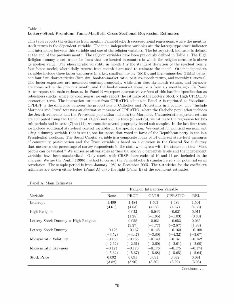
Table 11Lottery-Stock Premium: Fama-MacBeth Cross-Sectional Regression Estimates
This table reports the estimates from monthly Fama-MacBeth cross-sectional regressions, where the monthlystock return is the dependent variable. The main independent variables are the lottery-type stock indicatorand interaction between this variable and one of the religion variables. The lottery-stock indicator is definedat the end of the previous month. The religion variables have been previously defined in Table 1. The HighReligion dummy is set to one for firms that are located in counties in which the religion measure is aboveits median value. The idiosyncratic volatility in month t is the standard deviation of the residual from afour-factor model, where daily returns from month t are used to estimate the model. Other independentvariables include three factor exposures (market, small-minus-big (SMB), and high-minus-low (HML) betas)and four firm characteristics (firm size, book-to-market ratio, past six-month return, and monthly turnover).The factor exposures are measured contemporaneously, while firm size, six-month returns, and turnoverare measured in the previous month, and the book-to-market measure is from six months ago. In PanelA, we report the main estimates. In Panel B we report alternative versions of this baseline specification asrobustness checks, where for conciseness, we only report the estimate of the Lottery Stock × High CPRATIOinteraction term. The interaction estimate from CPRATIO column in Panel A is reprinted as “baseline”.CPDIFF is the difference between the proportions of Catholics and Protestants in a county. The “IncludeMormons and Jews” test uses an alternative measure of CPRATIO, where the Catholic population includesthe Jewish adherents and the Protestant population includes the Mormons. Characteristic-adjusted returnsare computed using the Daniel et al. (1997) method. In tests (5) and (6), we estimate the regression for twosub-periods and in tests (7) to (11), we consider several geography based sub-samples. In the last four tests,we include additional state-level control variables in the specification. We control for political environmentusing a dummy variable that is set to one for states that voted in favor of the Republican party in the lastPresidential elections. The Social Capital variable is a composite index of 14 different state-level measuresof community participation and the Trust variable is based on a question in the General Social Surveythat measures the percentage of survey respondents in the state who agrees with the statement that “Mostpeople can be trusted.” We winsorize all variables at their 0.5 and 99.5 percentile levels and the independentvariables have been standardized. Only stocks with CRSP share codes of 10 and 11 are included in theanalysis. We use the Pontiff (1996) method to correct the Fama-MacBeth standard errors for potential serialcorrelation. The sample period is from January 1980 to December 2005. The t-statistics for the coefficientestimates are shown either below (Panel A) or to the right (Panel B) of the coefficient estimates.
Panel A: Main Estimates
Religion Interaction Variable
Variable None PROT CATH CPRATIO REL
Intercept 1.499 1.484 1.503 1.489 1.501(4.61) (4.63) (4.57) (4.67) (4.63)
High Religion 0.023 −0.043 −0.021 0.011(1.25) (−1.85) (−1.03) (0.80)
Lottery Stock Dummy × High Religion 0.058 −0.031 −0.053 0.035(3.27) (−1.77) (−2.87) (1.88)
Lottery Stock Dummy −0.125 −0.167 −0.145 −0.160 −0.108(−3.52) (−4.47) (−3.80) (−4.32) (−3.67)
Idiosyncratic Volatility −0.156 −0.155 −0.149 −0.151 −0.152(−2.62) (−2.61) (−2.60) (−2.61) (−2.60)
Idiosyncratic Skewness −0.174 −0.176 −0.176 −0.175 −0.174(−5.62) (−5.67) (−5.68) (−5.65) (−5.64)
Stock Price 0.092 0.091 0.091 0.092 0.091(3.82) (3.96) (3.80) (3.99) (3.93)
Continued . . .
79

Table 11 – Continued from previous pageRobustness Checks: IPO First-Day Return Regression Estimates
Panel A: Main Estimates (Continued)
Religion Interaction Variable
Variable None PROT CATH CPRATIO REL
Market Beta 1.198 1.199 1.198 1.202 1.194(5.30) (5.32) (5.35) (5.34) (5.30)
SMB Beta 0.224 0.223 0.225 0.233 0.223(1.64) (1.65) (1.66) (1.75) (1.65)
HML Beta −0.606 −0.606 −0.603 −0.608 −0.605(−3.17) (−3.14) (−3.16) (−3.16) (−3.13)
Firm Size −0.460 −0.459 −0.456 −0.458 −0.459(−4.51) (−4.51) (−4.48) (−4.49) (−4.50)
Book-To-Market Ratio 0.144 0.145 0.146 0.146 0.143(2.26) (2.27) (2.31) (2.29) (2.24)
Past 12-Month Return 0.184 0.149 0.153 0.149 0.148(2.32) (2.38) (2.40) (2.39) (2.32)
Monthly Turnover −0.162 −0.166 −0.175 −0.171 −0.163(−1.26) (−1.28) (−1.41) (−1.33) (−1.24)
Average Number of Stocks 4,205 4,205 4,205 4,205 4,205Average Adjusted R2 0.057 0.060 0.059 0.059 0.058
Panel B: Estimates From Robustness Tests
CPRATIOTest Interaction t-statistic Avg N Avg Adj R2
Baseline −0.053 −2.87 4,205 0.059Basic Robustness(1) Use Ln(CPRATIO) instead of CPRATIO −0.054 −2.97 4,205 0.059(2) Use CPDIFF instead of CPRATIO −0.050 −2.74 4,205 0.059(3) Include Mormons and Jews −0.052 −2.74 4,205 0.058(4) Use Char-Adj Returns −0.052 −2.40 4,063 0.044Sub-Periods(5) 1980-1992 −0.038 −1.84 3,259 0.056(6) 1993-2005 −0.081 −3.07 5,155 0.062Geography-Based Sub-Samples(7) Exclude California −0.053 −2.73 3,869 0.059(8) Exclude North-East −0.040 −2.09 3,168 0.060(9) Exclude Mid-West −0.067 −3.24 3,429 0.062(10) Exclude South −0.044 −2.12 3,299 0.060(11) Exclude West −0.058 −2.87 3,311 0.061Additional Regional Controls(12) Control for Political Environment −0.053 −2.78 4,069 0.060(13) Control for Social Capital −0.052 −2.82 4,059 0.060(14) Control for Trust −0.049 −2.77 3,951 0.061(15) All Regional Controls −0.051 −2.70 3,951 0.062
80

Figure 1Geographical Variation in Religiosity and Religious Composition Across the U.S.
This figure shows the county-level religiosity (Panel A) and Catholic-Protestant ratio (Panel B) across theU.S. Each small outlined region in the figure corresponds to a county. In the top panel, darker shadeindicates more religious counties, while in the bottom panel, darker shade indicates counties with higherCatholic concentration. The county-level religion data are available for years 1980, 1990, and 2000 and thefigure shows the average religiosity and concentration measures for these three years.
Panel A: Religiosity Across the U.S.
Panel B: Catholic-Protestant Ratio Across the U.S.
81

Figure 2Religious Beliefs and Retail Investor Preference for Lottery-Type Stocks
This figure shows the average portfolio weights allocated to lottery-type stocks in the aggregate retail investorportfolio at a large U.S. discount brokerage house during the 1991 to 1996 period. Lottery-type stocksare defined as stocks with below-median price, above-median idiosyncratic volatility, and above-medianidiosyncratic skewness. The aggregate investor portfolio is created by combining the portfolios of all investorsin the sample. Investors are grouped into quintiles based on one of following three religion measures associatedwith the county of investor’s residence: Protestants (PROT), Catholics (CATH), and Catholic-Protestantratio (CPRATIO). PROT is the proportion of Protestant residents in the county where the investor resides,CATH is the proportion of Catholic residents in the investor’s county, and CPRATIO is the ratio of Catholicto Protestant residents in the investor’s county of residence. The figure shows the equal-weighted averagelottery stock weights for each religion quintile. The portfolio weights allocated to lottery-type stocks arecomputed each month and the graph reports the average values of those monthly weights.
Catholic Quintiles Protestant Quintiles Cath−Prot Ratio Quintiles8
9
10
11
12
13
14
County−Level Religion
Ret
ail W
eigh
t in
Lotte
ry−T
ype
Sto
cks
82