Embed Size (px)
Citation preview

INTERNATIONAL ECONOMIC REVIEWVol. 59, No. 2, May 2018 DOI: 10.1111/iere.12291
RELIGIONS, FERTILITY, AND GROWTH IN SOUTHEAST ASIA∗
BY DAVID DE LA CROIX AND CLARA DELAVALLADE 1
IRES, UCLouvain, Belgium, and CEPR; World Bank,Washington, USA
We investigate the extent to which the pronatalism of religions impedes growth via the fertility/educationchannel. Using Southeast Asian censuses, we show empirically that being Catholic, Buddhist, or Muslim signif-icantly raises fertility, especially for couples with intermediate to high education levels. With these estimates,we identify the parameters of a structural model. Catholicism is strongly pro-child (increasing total spendingon children), followed by Buddhism, whereas Islam is more pro-birth (redirecting spending from quality toquantity). Pro-child religions depress growth in its early stages by lowering savings and labor supply. In the laterstages of growth, pro-birth religions impede human capital accumulation.
1. INTRODUCTION
Many religions are theoretically pronatalist, to varying degrees. The Catholic doctrine pro-motes fertility by discouraging sexual intercourse other than for reproductive purposes, there-fore forbidding artificial birth control and abortion. Only natural family planning methods areallowed. The reluctance toward contraception builds upon the idea that men “must also rec-ognize that an act of mutual love which impairs the capacity to transmit life which God theCreator, through specific laws, has built into it, frustrates His design which constitutes the normof marriage, and contradicts the will of the Author of life.” (Encyclical Letter Humanae VitaeSection 13).2 In Islam, “procreation is a sign of God’s will and a large family is perceived as ablessing” (Blyth and Landau, 2009), although the Qur’an does not take a firm position on con-traception, leaving room for interpretation by local religious leaders. Buddhism’s sacred textsare more silent about family issues, but Buddhism also displays pro-family features: Guanyin,the Bodhisattva of compassion and mercy, is portrayed as a fertility goddess who has the powerto grant children, especially sons, and to ensure safe childbirth (Lee et al., 2009).
What implications do these beliefs have for economic growth? We know from empiricalstudies using microdata that belonging to a religious denomination indeed increases fertility.In addition, from the family economics literature, we know that there is a trade-off betweenfertility and education, that is, between the quantity of children and the quality of these children’seducation.3 Finally, the growth literature suggests that increased fertility may slow down humancapital accumulation through this trade-off, as well as physical capital accumulation, as in the
∗Manuscript received February 2016; revised March 2017.1 We thank Thomas Baudin, Sascha Becker, Bastien Chabe-Ferret, John Knowles, Paola Giuliano, Axel Gosseries,
Anastasia Litina, and Ester Rizzi for useful discussions on the article. The text also benefitted from comments atthe OLG days in Paris & Luxembourg, at the Barcelona GSE Summer Forum, at the SED 2016 conference, and atseminars in Bonn, Groningen, IRES (Louvain), GREQAM (Marseille), and UCLA. David de la Croix acknowledgesthe financial support of the project ARC 15/19-063 of the Belgian French-speaking Community. The views presented inthis paper are the authors’ and do not represent those of the World Bank or its member countries. All errors remain ourown. Please address correspondence to: David de la Croix, IRES, Universite Catholique Louvain, Place Montesquieu3, B-1348 Louvain-la-Neuve, Belgium. Phone: +32 1047 3453. E-mail: [email protected].
2 Similarly, “Children are really the supreme gift of marriage and contribute in the highest degree to their parents’welfare.” (Encyclical Letter Humanae Vitae Section 9). Although other Christian denominations have no centralauthority to diffuse this message across the world, they are also pronatalist, following the Bible’s commandment to “befruitful, and multiply” (Genesis 1:28).
3 See Doepke (2015) for a survey on the emergence of this concept.
907C© (2018) by the Economics Department of the University of Pennsylvania and the Osaka University Institute of Socialand Economic Research Association

908 DE LA CROIX AND DELAVALLADE
standard Solow model. The objective of this article is to link these three mechanisms andexamine the extent to which religion may affect growth through these channels. We first estimatethe impact of religion on fertility at the microeconomic level. We then map the identified effectinto a macroeconomic model to infer consequences for economic growth. Southeast Asiancountries provide the ideal environment to study this question since they host most of the majorworld religions in a small geographical area, allowing us to separate out country fixed effects(related to colonial origin, legal system, etc.) from religion fixed effects.
In our model, religion is not a choice, it is inherited from one’s parents. Religious affiliationsinfluence fertility behaviors by affecting households’ incentives. We assume that incentives areaffected by religion through preferences,4 whether these preferences result from ideology orwere shaped by socialization (Mosher et al., 1992).5 Looking through the lens of an optimalfertility model in which parents choose the number and the quality (health and level of edu-cation) of their children, we assume that religious values can affect fertility behaviors throughtwo different channels. A religion can be pro-child if it leads people to put more weight on thenumber and quality of children, as opposed to their own consumption and saving. It is pro-birthif it leads people to put more weight solely on the number of children with respect to the othercomponents of utility. We will see that these two features of religions affect the relationshipbetween parents’ education and their fertility differently.
To identify these theoretical channels, we need a method able to estimate the structuralparameters of a model that is nonlinear and implies cross-equation restrictions (some param-eters are assumed equal for all religions). We use indirect inference, a simulation methodthat allows estimating structural parameters from a standard fertility regression without im-posing a priori restrictions on the econometric model. Indirect inference follows a two-stepprocedure. We first estimate an auxiliary model to capture aspects of the data—here the ef-fect of parents’ education and religion on fertility—upon which the subsequent estimationof the structural model is based. One advantage of this auxiliary model is that it is directlycomparable to what one can find in the literature in demography and applied economics.Another advantage is drawing the moments used in the structural estimation from a singlecoherent sample, here the Integrated Public Use Micro Series, International (IPUMS-I) dataset. Second, we choose the parameters of the structural economic model such that they mini-mize the distance between the estimations of the parameters of the auxiliary model obtainedfrom the observed data and those obtained from artificial data simulated from the structuralmodel (Gourieroux et al., 1993; Smith, 2008). Once the parameters have been identified, weuse the structural model to simulate the influence of religion on growth. We then run exper-iments to compute the impact of religion on the growth process of artificial countries pop-ulated by nonreligious, Catholic, Buddhist, or Muslim inhabitants. We finally simulate theeffect of religion on the growth path of actual countries taking their religious composition intoaccount.
In the first step, we estimate the empirical relationship between parental background andfertility, including religion and education. Religion is modeled as affecting both the level offertility and the marginal effect of parents’ education on fertility. We use pooled census datafrom Southeast Asian countries for which religious affiliation is available as an individual vari-able (Cambodia, Indonesia, Malaysia, the Philippines, Thailand, and Vietnam). Southeast Asiais a particularly rich region in terms of religious affiliations both within and across countries:Catholics are present in the Philippines, as well as in Indonesia and Vietnam. Buddhists andMuslims are present in all the countries we study ( with the exception of Muslims in Vietnam).People with no religious affiliation are a majority in Vietnam and form small minorities ev-erywhere else. As we want to study the interaction effects of couples’ education and religion,
4 Using the World Value Survey, Guiso et al. (2003) show correlations between being raised religiously along differentdenominations and reported preferences and values regarding trust and gender equality.
5 A third view, according to which religion affects behavior through the minority status hypothesis, is implementedin Subsection 5.2.
RELIGIONS, FERTILITY, AND GROWTH 909
pooling censuses allows us to have enough observations in each category (for example, coupleswith no religious affiliation in which one spouse has a university degree and the other has noeducation).
Three main features emerge from the estimation of the empirical model. First, fertility de-creases as both men and women become more educated. Second, belonging to any religiousaffiliation (except Hinduism) raises fertility. Third, the effect of religion on fertility varies with acouple’s level of education. Catholicism has the strongest effect on fertility, but all predominantreligions raise fertility, especially for couples with intermediate and high levels of education.
In the second step, we estimate the parameters of a structural model of optimal fertility, usingthe fertility–religion relationship estimated in the first step as the “auxiliary” model. Comparedto calibration strategies that consist in exactly identifying the parameters from a set of momentsselected from various sources (two recent examples of calibrated fertility models are Doepkeet al., 2015, and Tamura et al., 2016), our moments are generated from the estimation of theauxiliary regression on a coherent set of data. Another difference with the calibrated modelsis that our moments have standard errors, enabling us to compute the standard errors of thestructural parameters, making it possible to measure the uncertainty surrounding both ourestimates and counterfactual simulations. We find that Catholicism clearly displays a pro-childeffect. Moreover, the fertility pattern of religious women points to strong pro-birth effects, inparticular for Muslim couples, and, to a lesser extent, for Buddhists and Catholics. This is truewhen one takes into account the interaction between religion and education in the auxiliarymodel: Highly educated couples with a religious denomination, and Muslims in particular, donot reduce their fertility as much as predicted by the behavior of nonreligious couples, as if thequantity–quality substitution mechanism were less at play for them.
The consequences for growth depend strongly on the size of the pro-birth effect. Indeed, ifreligion only increases the taste for children (pro-child), it leads to more spending on childrenand less saving. It depresses growth temporarily by lowering physical capital accumulation,but not human capital accumulation. These temporary effects account for 10% to 50% of theactual growth gaps between countries over 1950–1980. Conversely, if religion also decreases therelative weight of quality over quantity (pro-birth), it depresses growth permanently throughhuman capital accumulation. We show that countries with a large population affiliated to pro-birth religions have a lower human capital accumulation. In particular, religious compositionexplains between 10% and 20% of the gap between Muslim and Buddhist countries over 1980–2010.
These results cannot be fully compared with the existing literature, as this article is the firstto go all the way from microdata estimates to growth simulations. Qualitatively, our effects inthe auxiliary model are in line with the vast empirical literature at the microeconomic level thatshows that fertility choices can be heavily affected by partners’ religion and/or religiosity. Forexample, Sander (1992) shows that Catholic norms have a highly significant positive effect onfertility for respondents born before 1920 in the United Kingdom. Lin and Pantano (2015) showthat a mother’s religion affects the likelihood to have unintended birth(s) in the United States(using PSID data). Adsera (2006a, 2006b) shows that, in a secular society, religion predicts botha higher fertility norm and actual fertility. Baudin (2015) has similar findings on French data.Berman et al. (2018) show that fertility across European countries is related to the populationdensity of nuns, who are likely to provide services to families, alleviating child-rearing costs.
As far as developing countries are concerned, Heaton (2011) studies the effect of religionon fertility in a set of 22 developing countries using survey data. He shows that the level ofeducational achievements matter for this relationship, stressing the importance of interactioneffects, which is also a conclusion of our auxiliary model. Chabe-Ferret (2016) shows thatreligious affiliation is a substantial channel through which cultural norms affect fertility choicesof second-generation migrants in France. In particular, controlling for religion reduces theeffect of the fertility norms from the origin country. Finally, Skirbekk et al. (2015) study theeffect of Buddhism in several Asian countries and claim that it is the least pronatalist religion.Although most of these studies control for the education level of mothers, few of them control

910 DE LA CROIX AND DELAVALLADE
for the education level of fathers, and none of them allows, as we do, for an interaction betweeneducation and religion.
There is also an empirical literature at the macroeconomic level linking religion to educationand growth. The debate goes back at least to Weber, who praised the virtues of Protestantethics for economic growth. Along Weberian lines, Becker and Woessmann (2009) and Boppartet al. (2013) show that Protestantism led to better education than Catholicism in 19th-centuryPrussian counties and in Swiss districts. This difference between Catholics and Protestants is,however, not visible in our study. It should be noted though that Protestantism is far fromuniform. McCleary (2013) compares Protestant missionaries in Korea and Guatemala andshows that their approach to exporting Protestantism was different, with a focus on educationin Korea from mainline denominations, but little investment in human capital in Guatemalafrom fundamentalist denominations. Finally, using contemporaneous data, Barro and McCleary(2003) attempt to isolate the direction of causation from religiosity to economic performanceand find a negative effect of religious practice on growth; however, their results are shown notto be robust by Durlauf et al. (2006).
Several authors propose growth models embedding religious considerations. Some, like us,consider religion exogenous. Cavalcanti et al. (2007) explicitly model an afterlife period (heavenor hell) in an overlapping generation setup, and show that beliefs about how to maximize one’schances to go to heaven affect capital accumulation. Strulik (2012) defends the view thatreligion may affect preferences, either for fertility or leisure (individuals with “religious” valuesattach a lower weight to consumption utility than those with “secular” values). Comparedto our model in which religion is treated as an exogenous difference in the parameters, theinterest of Strulik (2012) is to make religious affiliation endogenous. Endogenous religion isalso modeled by Baudin (2010), who studies the joint dynamics of cultural values and fertilityand shows the conditions under which a demographic transition accompanied by a rise in“modern” (vs. “traditional”) culture happens. Finally, Cervellati et al. (2014) model religionas an insurance against idiosyncratic shocks and determine which system of religious norms isincentive compatible. They explicitly show that individual incentives are modified by religiousnorms, which is what we implicitly assume when we make preferences depend directly onreligious affiliation. None of these theoretical models, however, provides a quantitative measureof their implications disciplined by microeconometric estimates.
The remainder of the article is organized as follows: Section 2 presents and estimates theauxiliary model of fertility. We develop the structural model in Section 3. Section 4 uses agrowth model to infer dynamic and long-run implications of religion on fertility, education, andgrowth. Section 5 presents robustness analysis. Section 6 concludes.
2. THE AUXILIARY MODEL
We specify an auxiliary model to estimate the marginal effects of education on fertility. Thisin turn will be used to estimate the parameters of the structural economic model such that thedistance between these empirical marginal effects and those obtained from the structural modelis minimal.
2.1. Data and Empirical Strategy. Our empirical analysis uses data from the IntegratedPublic Use Micro Series, International (IPUMS-I) Minnesota Population Center (2013). TheIPUMS-I census microdata are unique in providing internationally comparable, detailed infor-mation on demographics, religion, and education. We restrict our analysis to Southeast Asiabecause it covers a variety of religions while still having common historical, cultural, and geo-graphical influences,6 thus reducing the noise inherent to a cross-country analysis. Harmonizeddata for Southeast Asia come from 11 censuses collected by national statistical agencies in
6 According to Putterman (2006), the transition to agriculture took place from 6000 (Vietnam) to 4000 (Indonesia)before present. Following Alesina et al. (2013), the plough was used in pre-historical times in all six countries considered,
RELIGIONS, FERTILITY, AND GROWTH 911
1900 1910 1920 1930 1940 1950 1960
Cambodia
Indonesia
Malaysia The Philippines
Vietnam
Thailand
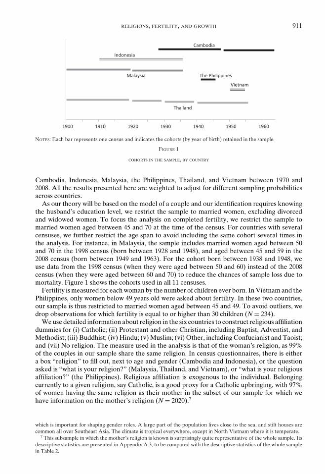
NOTES: Each bar represents one census and indicates the cohorts (by year of birth) retained in the sample
FIGURE 1
COHORTS IN THE SAMPLE, BY COUNTRY
Cambodia, Indonesia, Malaysia, the Philippines, Thailand, and Vietnam between 1970 and2008. All the results presented here are weighted to adjust for different sampling probabilitiesacross countries.
As our theory will be based on the model of a couple and our identification requires knowingthe husband’s education level, we restrict the sample to married women, excluding divorcedand widowed women. To focus the analysis on completed fertility, we restrict the sample tomarried women aged between 45 and 70 at the time of the census. For countries with severalcensuses, we further restrict the age span to avoid including the same cohort several times inthe analysis. For instance, in Malaysia, the sample includes married women aged between 50and 70 in the 1998 census (born between 1928 and 1948), and aged between 45 and 59 in the2008 census (born between 1949 and 1963). For the cohort born between 1938 and 1948, weuse data from the 1998 census (when they were aged between 50 and 60) instead of the 2008census (when they were aged between 60 and 70) to reduce the chances of sample loss due tomortality. Figure 1 shows the cohorts used in all 11 censuses.
Fertility is measured for each woman by the number of children ever born. In Vietnam and thePhilippines, only women below 49 years old were asked about fertility. In these two countries,our sample is thus restricted to married women aged between 45 and 49. To avoid outliers, wedrop observations for which fertility is equal to or higher than 30 children (N = 234).
We use detailed information about religion in the six countries to construct religious affiliationdummies for (i) Catholic; (ii) Protestant and other Christian, including Baptist, Adventist, andMethodist; (iii) Buddhist; (iv) Hindu; (v) Muslim; (vi) Other, including Confucianist and Taoist;and (vii) No religion. The measure used in the analysis is that of the woman’s religion, as 99%of the couples in our sample share the same religion. In census questionnaires, there is eithera box “religion” to fill out, next to age and gender (Cambodia and Indonesia), or the questionasked is “what is your religion?” (Malaysia, Thailand, and Vietnam), or “what is your religiousaffiliation?” (the Philippines). Religious affiliation is exogenous to the individual. Belongingcurrently to a given religion, say Catholic, is a good proxy for a Catholic upbringing, with 97%of women having the same religion as their mother in the subset of our sample for which wehave information on the mother’s religion (N = 2020).7
which is important for shaping gender roles. A large part of the population lives close to the sea, and stilt houses arecommon all over Southeast Asia. The climate is tropical everywhere, except in North Vietnam where it is temperate.
7 This subsample in which the mother’s religion is known is surprisingly quite representative of the whole sample. Itsdescriptive statistics are presented in Appendix A.3, to be compared with the descriptive statistics of the whole samplein Table 2.
912 DE LA CROIX AND DELAVALLADE
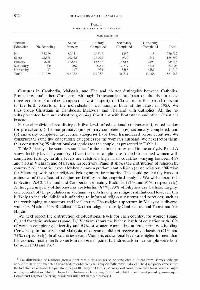
TABLE 1SAMPLE SIZE, BY COUPLE EDUCATION
Man Education
WomanEducation No Schooling
SomePrimary
PrimaryCompleted
SecondaryCompleted
UniversityCompleted Total
No 155,029 89,151 24,542 1392 113 270,227Some 13,978 109,132 38,078 4930 541 166,659Primary 2235 16,874 55,567 14,065 2097 90,838Secondary 100 1058 5234 12,779 3834 23,005University 17 117 936 3568 6581 11,219Total 171,359 216,332 124,357 36,734 13,166 561,948
Censuses in Cambodia, Malaysia, and Thailand do not distinguish between Catholics,Protestants, and other Christians. Although Protestantism has been on the rise in thesethree countries, Catholics composed a vast majority of Christians in the period relevantto the birth cohorts of the individuals in our sample, born at the latest in 1963. Wethus group Christians in Cambodia, Malaysia, and Thailand with Catholics. All the re-sults presented here are robust to grouping Christians with Protestants and other Christiansinstead.
For each individual, we distinguish five levels of educational attainment: (i) no education(or pre-school); (ii) some primary; (iii) primary completed; (iv) secondary completed; and(v) university completed. Education categories have been harmonized across countries. Weconstruct the same five educational categories for the woman’s husband. We next factor them,thus constructing 25 educational categories for the couple, as presented in Table 1.
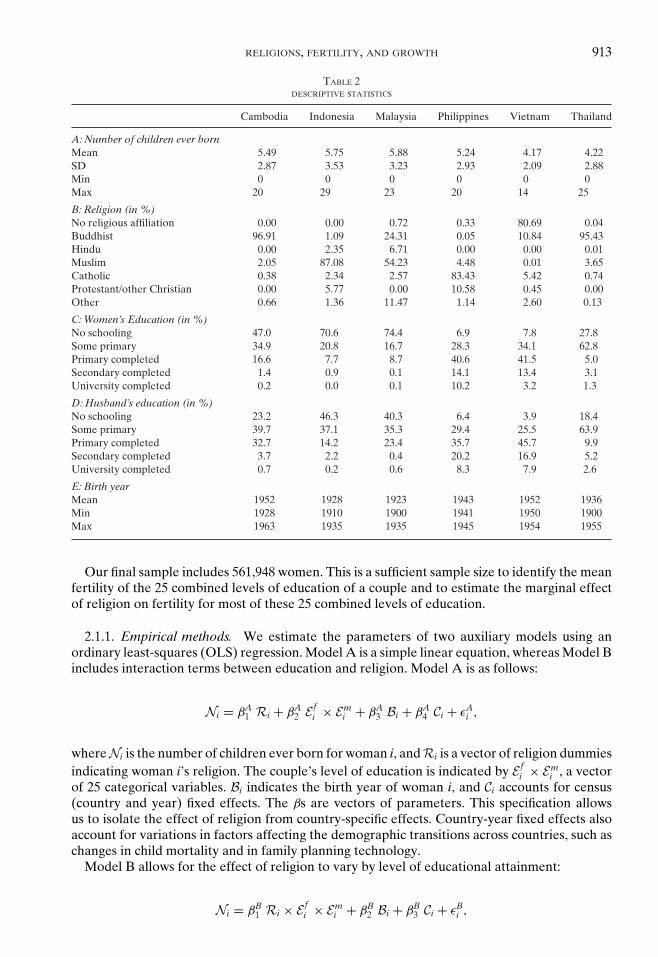
Table 2 displays the summary statistics for the main measures used in the analysis. Panel Ashows fertility levels by country. Given that our sample is restricted to married women withcompleted fertility, fertility levels are relatively high in all countries, varying between 4.17and 5.88 in Vietnam and Malaysia, respectively. Panel B shows the distribution of religion bycountry.8 All countries except Malaysia have a predominant religion (or no religious affiliationfor Vietnam), with other religions belonging to the minority. This could potentially bias ourestimates of the effect of religion on fertility in the empirical analysis. We will discuss thisin Section A.4.2. Thailand and Cambodia are mainly Buddhist (97% and 95%, respectively).Although a majority of Indonesians are Muslim (87%), 83% of Filipinos are Catholic. Eighty-one percent of the population in Vietnam reports having no religious affiliation. However, thisis likely to include individuals adhering to informal religious customs and practices, such asthe worshipping of ancestors and local spirits. The religious spectrum in Malaysia is diverse,with 54% Muslim, 24% Buddhist, 11% other religions, mostly Confucianist and Taoist, and 7%Hindu.
We next report the distribution of educational levels for each country, for women (panelC) and for their husbands (panel D). Vietnam shows the highest levels of education with 10%of women completing university and 65% of women completing at least primary schooling.Conversely, in Indonesia and Malaysia, most women did not receive any education (71% and74%, respectively). In all countries except Vietnam, educational levels are higher for men thanfor women. Finally, birth cohorts are shown in panel E: Individuals in our sample were bornbetween 1900 and 1963.
8 The distribution of religious groups from census data seems to be somewhat different from Barro’s religiousadherence data: http://scholar.harvard.edu/files/barro/files/7_religion_adherence_data.xls. The discrepancy comes fromthe fact that we consider the population aged 40+ only and that, in some special cases, there have been recent changesin religious affiliation (children from Catholic families becoming Protestants, children of atheist parents growing up inCommunist regimes declaring themselves Buddhist in recent surveys).
RELIGIONS, FERTILITY, AND GROWTH 913
TABLE 2DESCRIPTIVE STATISTICS
Cambodia Indonesia Malaysia Philippines Vietnam Thailand
A: Number of children ever bornMean 5.49 5.75 5.88 5.24 4.17 4.22SD 2.87 3.53 3.23 2.93 2.09 2.88Min 0 0 0 0 0 0Max 20 29 23 20 14 25
B: Religion (in %)No religious affiliation 0.00 0.00 0.72 0.33 80.69 0.04Buddhist 96.91 1.09 24.31 0.05 10.84 95.43Hindu 0.00 2.35 6.71 0.00 0.00 0.01Muslim 2.05 87.08 54.23 4.48 0.01 3.65Catholic 0.38 2.34 2.57 83.43 5.42 0.74Protestant/other Christian 0.00 5.77 0.00 10.58 0.45 0.00Other 0.66 1.36 11.47 1.14 2.60 0.13
C:Women’s Education (in %)No schooling 47.0 70.6 74.4 6.9 7.8 27.8Some primary 34.9 20.8 16.7 28.3 34.1 62.8Primary completed 16.6 7.7 8.7 40.6 41.5 5.0Secondary completed 1.4 0.9 0.1 14.1 13.4 3.1University completed 0.2 0.0 0.1 10.2 3.2 1.3
D:Husband’s education (in %)No schooling 23.2 46.3 40.3 6.4 3.9 18.4Some primary 39.7 37.1 35.3 29.4 25.5 63.9Primary completed 32.7 14.2 23.4 35.7 45.7 9.9Secondary completed 3.7 2.2 0.4 20.2 16.9 5.2University completed 0.7 0.2 0.6 8.3 7.9 2.6
E: Birth yearMean 1952 1928 1923 1943 1952 1936Min 1928 1910 1900 1941 1950 1900Max 1963 1935 1935 1945 1954 1955
Our final sample includes 561,948 women. This is a sufficient sample size to identify the meanfertility of the 25 combined levels of education of a couple and to estimate the marginal effectof religion on fertility for most of these 25 combined levels of education.
2.1.1. Empirical methods. We estimate the parameters of two auxiliary models using anordinary least-squares (OLS) regression. Model A is a simple linear equation, whereas Model Bincludes interaction terms between education and religion. Model A is as follows:
Ni = βA1 Ri + βA
2 E fi × Em
i + βA3 Bi + βA
4 Ci + εAi ,
whereNi is the number of children ever born for woman i, andRi is a vector of religion dummiesindicating woman i’s religion. The couple’s level of education is indicated by E f
i × Emi , a vector
of 25 categorical variables. Bi indicates the birth year of woman i, and Ci accounts for census(country and year) fixed effects. The βs are vectors of parameters. This specification allowsus to isolate the effect of religion from country-specific effects. Country-year fixed effects alsoaccount for variations in factors affecting the demographic transitions across countries, such aschanges in child mortality and in family planning technology.
Model B allows for the effect of religion to vary by level of educational attainment:
Ni = βB1 Ri × E f
i × Emi + βB
2 Bi + βB3 Ci + εB
i ,
914 DE LA CROIX AND DELAVALLADE
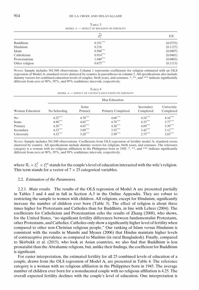
TABLE 3MODEL A — EFFECT OF RELIGION ON FERTILITY
βA1 S.E.
Buddhism 0.331*** (0.0725)Hinduism 0.218 (0.1127)Islam 0.560*** (0.0907)Catholicism 0.914*** (0.0461)Protestantism 1.040*** (0.0803)Other religion 0.675*** (0.1113)
NOTES: Sample includes 561,948 observations. Column 1 represents coefficients for religion estimated with an OLSregression of Model A; standard errors clustered by country in parentheses in column 2. All specifications also includedummy vectors for combined education levels of couples, birth years, and censuses. *, **, and *** indicate significantlydifferent from zero at 90%, 95%, and 99% confidence intervals, respectively.
TABLE 4MODEL A — EFFECT OF COUPLE’S EDUCATION ON FERTILITY
Man Education
Woman Education No SchoolingSome
Primary Primary CompletedSecondaryCompleted
UniversityCompleted
No 4.25*** 4.78*** 4.66*** 4.54*** 4.16***
Some 4.90*** 4.82*** 4.70*** 4.33*** 3.77***
Primary 4.26*** 4.65*** 4.36*** 4.09*** 3.39***
Secondary 4.23*** 3.89*** 3.52*** 3.42*** 3.12***
University 4.32*** 3.28*** 2.99*** 2.75*** 2.83***
NOTES: Sample includes 561,948 observations. Coefficients from OLS regression of fertility model A; standard errorsclustered by country. All specifications include dummy vectors for religions, birth years, and censuses. The referencecategory is a woman with no religious affiliation in the Philippines born in 1945. *, **, and *** indicate significantlydifferent from zero at 90%, 95%, and 99% confidence intervals, respectively.
whereRi × E fi × Em
i stands for the couple’s level of education interacted with the wife’s religion.This term stands for a vector of 7 × 25 categorical variables.
2.2. Estimation of the Parameters.
2.2.1. Main results. The results of the OLS regression of Model A are presented partiallyin Tables 3 and 4 and in full in Section A.5 in the Online Appendix. They are robust torestricting the sample to women with children. All religions, except for Hinduism, significantlyincrease the number of children ever born (Table 3). The effect of religion is about threetimes higher for Protestants and Catholics than for Buddhists, in line with Lehrer (2004). Thecoefficients for Catholicism and Protestantism echo the results of Zhang (2008), who shows,for the United States, “no significant fertility differences between fundamentalist Protestants,other Protestants, and Catholics. Catholics only show a significantly higher level of fertility whencompared to other non-Christian religious people.” Our ranking of Islam versus Hinduism isconsistent with the results in Munshi and Myaux (2006) that Hindus maintain higher levelsof contraceptive prevalence as compared to Muslims (in rural Bangladesh). Finally, comparedto Skirbekk et al. (2015), who look at Asian countries, we also find that Buddhism is lesspronatalist than the Abrahamic religions, but, unlike their findings, the coefficient for Buddhismis significant.
For easier interpretation, the estimated fertility for all 25 combined levels of education of acouple, drawn from the OLS regression of Model A, are presented in Table 4. The referencecategory is a woman with no religious affiliation in the Philippines born in 1945. The averagenumber of children ever born for a noneducated couple with no religious affiliation is 4.25. Theoverall expected fertility declines with the couple’s level of education. One interpretation is

RELIGIONS, FERTILITY, AND GROWTH 915
that the time spent on child care becomes more expensive when people are more productive.The higher value of time raises the cost of children, thereby reducing the demand for largefamilies (Becker, 1993). The average is 2.83 for a couple in which both spouses have a universitydegree. Interestingly though, among couples with low education, fertility is slightly higher forthose in which at least one of the spouses has received some primary education. This suggeststhat, for low levels of education, additional years of schooling translate into higher income,thus alleviating the cost of child rearing and translating into higher fertility. For couples with aneducational level higher than primary school, the opportunity cost of child rearing compensatesthis effect, however, causing fertility to decline with years of schooling.
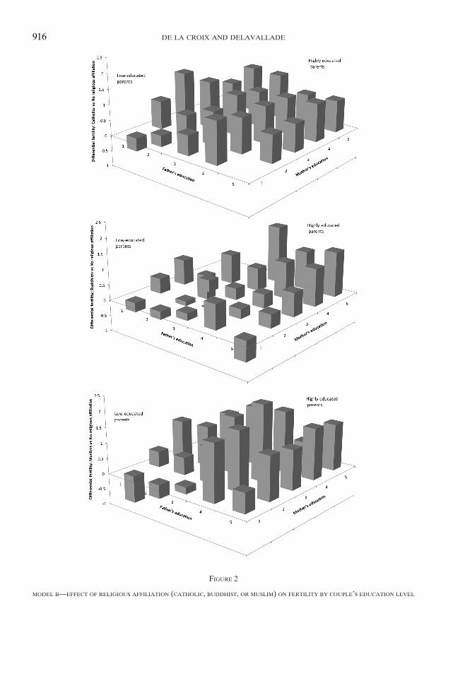
We next turn to the OLS estimation of Model B in which we regress fertility on the 25education couples, on education couples interacted with all religions, as well as on censusand birth year dummies. The full results are presented in Table A.5 in the Online Appendix,and the resulting moments used for estimation are in Appendix A.7.1. In Figure 2, we onlypresent estimates of the marginal effect of being Catholic (respectively, Buddhist or Muslim)instead of nonreligious on fertility at each educational level. For each religion, the coupleswith low education are on the left and those with high education on the right. Allowing theimpact of religion to vary across educational levels shows a more complex picture than theone shown by Model A, with three main features. First, the marginal effect of Catholicism onfertility (top panel) is stronger for couples with middle to high levels of education (completedprimary or secondary). A Catholic couple who completed primary education has on average1.29 more children than a couple without religious affiliation (a difference of 33% in thenumber of children), whereas for couples with no education, the effect is negligible (evennegative). This implies that this religious affiliation tends to dampen the decline in fertility dueto education. Second, the main feature highlighted for Catholicism is also true for Buddhism(middle panel). However, there are differences with the patterns highlighted for the marginaleffects of Catholicism at varying education levels. The marginal effects of Buddhism on fertilityare overall lower in magnitude than the effects of Catholicism, in line with estimates fromModel A (Table 4). Buddhism has the strongest positive impact on the fertility of coupleswith the highest levels of education (secondary schooling and above). A Buddhist womanin a couple in which both spouses hold a university degree has 1.44 more children than onewithout religious affiliation (62% more), whereas there is no significant difference between aBuddhist and a woman without religious affiliation in noneducated couples (with 5.58 childrenon average). Third, looking at Islam (bottom panel), we also find that educated couples’ fertilityis more affected by being religious than that of less educated couples. The effect is particularlystrong for fathers and mothers with secondary education or more and is even stronger for Islamthan for Catholicism.
Note finally that, in Figure 2, some coefficients are based on a very small number of obser-vations.9 When estimating the structural parameters of the model we will develop in the nextsection, we discard estimates based on less than 30 observations.10
We compute an F -statistic to compare both models. The F -statistic is 2233 with a p-value of0.00, leading to a rejection of the null hypothesis that Model B does not provide a significantlybetter fit than Model A.
2.2.2. Additional tests. In this subsection, we discuss and test the robustness of the estimationof the auxiliary model presented above.
Our dependent variable, fertility, is a count variable, taking values between 0 and 29. Sincethe distribution of residuals is not normal, applying a linear regression model might lead toinefficient and inconsistent estimates (Long and Freese, 2006) but allows us to directly interpret
9 Note that our sample only counts 17 couples in which the woman has a university degree whereas her husband hasno education and 113 couples in which the woman has no education whereas her husband has a university degree.
10 Cells (i)×(iv), (i)×(v), (iv)×(i), and (v)×(i) for people without religious affiliation, (i)×(v), (iv)×(i), and (v)×(i)for Catholics, (v)×(i) and (v)×(ii) for Buddhists, (iv)×(i), (v)×(ii), and (v)×(iii) for Muslims.
916 DE LA CROIX AND DELAVALLADE
FIGURE 2
MODEL B—EFFECT OF RELIGIOUS AFFILIATION (CATHOLIC, BUDDHIST, OR MUSLIM) ON FERTILITY BY COUPLE’S EDUCATION LEVEL
RELIGIONS, FERTILITY, AND GROWTH 917
the results in terms of number of children. To assess the robustness of our main estimations,we estimate Models A and B with a Poisson regression. The results are presented in Table A.5in the Online Appendix (columns 2 and 4). The significance of the coefficients is not weakenedby substituting Poisson for OLS estimations. Moreover, the size of the effects are very similar.For example, considering the coefficients presented in Table 3, the Poisson estimation leads tothe following estimates of the marginal effect of each religion: 0.336, 0.269, 0.565, 0.910, 0.995,and 0.654. The only difference is that the coefficient related to Hinduism is now significant.
An additional concern is that the impact of religion (and of religion interacted with education)may vary between countries. In fact, our estimation provides an estimation of the average effectof religions on fertility in Southeast Asia. To account for country-specific effects of religions,one option would be to incorporate dummy variables interacting country and religion (andcountry, religion, and education), but this puts too many constraints on the model and preventsus from estimating the standard errors of the coefficients. Nevertheless, to evaluate whether theestimation results are driven by a particular country, we estimate Models A and B with restrictedsamples. Section A.6 of the Online Appendix presents the results from these regressions. Foreasier comparison, columns 1 and 2 report results from the main OLS regressions using thefull sample presented earlier (in Section A.5). The sample excludes the Philippines, mostlyCatholic, in columns 3 and 4, and Thailand, predominantly Buddhist, in columns 5 and 6.Although the specification is identical to that described above, we do not report the estimatesof the educational category, census, and birth year coefficients for better readability. The resultsusing the three different samples are very similar. Being a Catholic, as opposed to not having areligious affiliation, brings an additional 0.88 child on average when the Philippines or Thailandare excluded from the sample, compared to an additional 0.91 child on average with the fullsample. The positive impact of being Hindu is significant in the models estimated with therestricted samples. Finally, the estimates of the marginal effect of religion at different levels ofcouples’ education are very similar across all three samples.
Another potential limitation is that education might be endogenous to fertility due to teenagepregnancies. Restricting our sample to women aged over 20 at the time of their first child’s birth,instrumenting for age at menarche (Ribar, 1994) or for miscarriage (Hotz et al., 2005), wouldallow us to rule out this argument, but this information is not available in the IPUMS data.
Finally, the robustness of the results to the inclusion of variables reflecting the minority statushypothesis is analyzed in Subsection 5.2.
3. THE STRUCTURAL MODEL
We now estimate the structural parameters of an economic model with a quality–quantitytrade-off. We identify these parameters with an indirect inference method, using the fertilityequation from Section 2 as the auxiliary model. The structural model we use is the one proposedby de la Croix and Doepke (2003), extended to allow for different sources of income and optimaldegrees of involvement in child rearing from the father and mother (inspired by Bar et al., 2017).It is a very parsimonious model that captures one key feature: Since the time cost of rearingchildren is higher for more educated parents, they prefer having fewer children but investingmore in their quality. A critical assumption of this model is that the most important cost ofhaving children is a time cost instead of a good cost (see the estimation of Cordoba and Ripoll,2016, for the United States).
As stated in the introduction, we view religion as exogenous and affecting household prefer-ences and thereby their incentives. We focus on four types of hypothetical households: Catholic,Buddhist, Muslim, and without religious affiliation. These are the religions for which we haveenough individuals in each educational cell to be confident in the estimation of Model B de-scribed above.
Note that we could alternatively assume that religions modify the household technology—for example, by affecting the good cost needed to raise and/or to educate one child. In thatcase, preferences can be identical across all households, but technology differs by religion.
918 DE LA CROIX AND DELAVALLADE
For example, a feature of Catholicism is that churches are also involved in education. PrivateCatholic schooling is common around the world, and it is generally subsidized. One couldthen rationalize Catholicism as being pro-child because highly educated parents are able tospend more on both the quantity and quality of children, since the Church provides relativelycheap access to private schooling. From this perspective, it may not be that Catholic parentshave a high weight on the quality of children embedded in their preferences (high η in themodel), but that subsidized private schooling allows parents to educate more children. In fact,we cannot distinguish between household technology and preferences. Observationally, thetwo approaches are equivalent, but the interpretation in terms of preferences is in line with theliterature on religion as a cultural trait (Bisin and Verdier, 2010). Both interpretations implythat religions modify incentives, which is what we measure in the first-order conditions of thehousehold maximization problem, either through preference parameters and shadow prices orthrough technology and actual costs.
3.1. Households’ Problem. Consider a hypothetical economy populated by overlapping gen-erations of individuals with the same religion who live over three periods: childhood, adulthood,and old age. All decisions are made in the adult period of their life. Households care aboutadult consumption ct, old-age consumption dt+1, their number of children nt, and their quality(human capital) ht+1. They have the same preferences and act cooperatively (unitary model ofthe household). Their utility function is given by
ln(ct) + σ ln(dt+1) + γ ln(nth
η
t+1
).(1)
The parameter σ > 0 is the psychological discount factor, and γ > 0 is the weight of childrenin the utility function. Parameter η ∈ (0, 1) is the weight of the quality versus the quantity ofchildren for the household. The budget constraint for a couple with human capital (hf
t , hmt ) is
ct + st + etntwthT = ωwthft
(1 − af
t nt
)+ wthm
t (1 − amt nt) ,(2)
where wt is the wage per unit of human capital, and ω is an exogenous gender wage gap (due,for example, to discrimination). af
t and amt are the time parents spend on child rearing. The total
educational cost per child is given by ethT, where et is the number of hours of teaching boughtfrom a teacher with human capital hT. The assumption that teachers are potentially differenthuman capital than parents is similar to Tamura (2001). When coupled with the assumption thatthere is a minimum time cost required to bear children, it implies that highly educated parentswill spend more on the quality of their children (de la Croix and Doepke, 2003; Moav, 2005).
The technology that allows people to produce children is given by11
nt = 1φ
√af
t amt .(3)
It stresses that time is essential to produce children and that the mother’s and father’s time aresubstitutes. We do not introduce an a priori asymmetry between parents. Asymmetry will ariseas an equilibrium phenomenon: With the gender wage gap ω < 1, it will be optimal to havethe mother spend more time on child rearing. The parameter φ ∈ (0, 1) gives an upper boundto the number of children. If both parents devote their entire time to producing children, theywill get 1/φ of them. As is clear from (3), we abstract from the uncertainty on child production.The two main sources of uncertainty we abstract from are child mortality (for the differentways to introduce child mortality into similar models, see Doepke, 2005), young adult mortality
11 Adapted from Browning et al. (2014, p. 265), and Gobbi (2018) to the production of quantity instead of quality.

RELIGIONS, FERTILITY, AND GROWTH 919
(see Tamura, 2006), and family planning failures (see Bhattacharya and Chakraborty, 2013, formodeling them).
The budget constraint for the old-age period is
dt+1 = Rt+1st.(4)
Rt+1 is the interest factor. Children’s human capital ht+1 depends on their education et:
ht+1 = μt(θ + et)ξ.(5)
The presence of θ > 0 guarantees that parents have the option of not educating their children,because even with et = 0, future human capital remains positive. It can be interpreted as the levelof public education provided to parents for free. Parameter ξ is the elasticity of human capitalto education. It is to be understood as determining the rate of return on parental investmentin education. The parents’ influence on their children’s human capital is limited to the effectthrough education spending. The specification of the efficiency parameter μt does not affectindividual choices and is left to the next section.
The household maximization problem is solved in Appendix A.1. For a household whosehuman capital is high enough to ensure that the opportunity cost of an additional child is high,such that
ωhft hm
t >
(θhT
2φηξ
)2
,(6)
there is an interior solution with positive spending on education. For households with lowerhuman capital, the optimal choice for education et is zero. Education and fertility decisions canbe summarized by
et = max
⎡⎣0,2φηξ
√ωhf
t hmt − θhT
(1 − ηξ)hT
⎤⎦ ,(7)
nt = max
⎡⎣ γ(ωhf
t + hmt
)2(1 + σ + γ)φ
√ωhf
t hmt
,(1 − ηξ)γ
(ωhf
t + hmt
)1 + σ + γ
2φ
√ωhf
t hmt + θhT
4φ2ωhft hm
t − θ2hT2
⎤⎦ .(8)
In the corner regime (first terms in the max), there is no trade-off between the quality andquantity of children. In the interior regime, the second terms inside the max reflect the quality–
quantity trade-off: When the opportunity cost of raising children φ
√ωhf
t hmt increases, parents
substitute education et for quantity nt. There is strong empirical evidence that this mechanismis at work in developing countries (see, e.g., the study on Chinese twins by Li et al., 2008, andthe one by Klemp and Weisdorf, 2018, on pre-industrial England). This substitution only occursin the interior regime.
We now use these equations to interpret the effect of religion on individual choices. Weconsider here that religion is exogenous and implies different preference parameters acrossdenominations and compared to nonreligious people. We assume that religion neither influencesthe time cost parameter φ, the constant θ, nor the rate of return on education ξ. φ flows from atechnological constraint. θ represents the provision of education good (possibly public) imposedon the parents. ξ depends on the labor market in each country. We focus on the two parametersthat most likely depend on religious values.

920 DE LA CROIX AND DELAVALLADE
If a religion increases the preference for children γ, it leads to more children, the same levelof education per child, and less saving. This holds both in the interior regime and in the cornerregime. It may thus depress growth through physical capital accumulation, but not throughhuman capital accumulation. We will call this religion pro-child since it promotes both quantityand quality.
If a religion decreases the relative weight of quality over quantity η, it has no effect in thecorner regime. In the interior regime, it leads to more children, less education, and the samelevel of saving. It may therefore depress growth through human capital accumulation. Such areligion is said to be pro-birth.
The two notions we introduce, pro-child and pro-birth, describe how households that increasethe share of children in total spending actually spend that income. Coming back to the budgetconstraint (A.2), the total spending on children can be decomposed into spending on qualityand spending on quantity. Using the first-order conditions in the interior regime, we can seehow these two spending shares are directly expressed in terms of the parameters γ and η whenθ is small:
Spending on quality:etnthT
ωhft + hm
t
= γηξ
1 + γ + σfor θ = 0.
(opportunity) Cost on quantity:2φ
√ωhf
t hmt n
ωhft + hm
t
= γ(1 − ηξ)1 + γ + σ
for θ = 0.
Hence a pro-child religion (high γ) leads to more spending of the two types, whereas a pro-birthreligion (low η) redirects spending from quality toward quantity.12
3.2. Identification. One period is assumed to be 30 years. Some parameters are set a priori,based on commonly accepted values, supposed common to all countries. The biological time costof raising children per couple is φ = 0.065, implying a maximum number of children per coupleof �1/φ� = 15. The discount factor σ is set at 1% per quarter, that is, σ = 0.99120 = 0.3. The rateof return on education spending ξ is set to 1/3. As we can see from the first-order conditions, itcannot be identified separately from η; hence it can be seen as a scaling factor on η. Parameterξ is related to the Mincerian rate of return � (defined by ht+1 = exp(� × years of education))through the following relation:
� = d ln ht+1
dede
d(years of education),
where de/d(years of education) represents the increase in educational spending needed to in-crease the number of years of education by one. Assuming as in de la Croix and Doepke(2003) that an additional year of schooling raises educational expenditure by 20% and usingthe first-order condition for e in the interior regime, we get
� = ξ
θ + e0.2 e,
which leads to � = 0.066 for θ negligible. A Mincerian return of 6.6% seems a reasonablyconservative estimate for emerging countries.
12 The logarithmic utility is essential to obtain these simple expressions. Assuming a more general utility with anelasticity of substitution between goods different from unity would lead to more complicated expressions, with spendingshares depending on the shadow prices of the quantity and quality of children. Except for the Barro–Becker approach,which develops a model of optimal fertility with rational altruism and infinite horizon, the rest of the literature assumeslogarithmic utility, reflecting that there is little to gain in terms of insights by having more complicated functional forms.
RELIGIONS, FERTILITY, AND GROWTH 921
TABLE 5INCOME BY EDUCATION CATEGORY IN THE PHILIPPINES
No Education Some Primary Primary Completed Secondary Completed University Completed
hf 1 1.035 1.07 1.46 2.14hm 1 1.065 1.13 1.37 1.86
NOTE: Estimations from Luo and Terada (2009). Results normalized to 1 for category (i).
To compute the fertility of the 25 types of couples in Table 1, we need to map educationallevels into earnings levels. We use the study of Luo and Terada (2009), who estimate the earningsof men and women of different educational categories in the Philippines. The advantage of thisstudy is that the categories of education they use map perfectly with those of IPUMS-I . Theyfind that the gender wage gap for low educational levels is ω = 0.75. Table 5 shows the humancapital level for all educational categories. Women’s income is given by ωhf .
The Mincerian rate of return implicit in Table 5 depends on whether education includes yearsof primary education or not. Including years of primary education leads to low estimates of �.For example, for women,13 assuming that one needs 16 years to complete university, we have2.14 = exp(�16), leading to � = 4.7%. Computing the rate of return once primary education iscompleted leads to higher estimates: 2.14/1.07 = exp(�(16 − 6)), that is, � = 6.9%.
An alternative way of measuring human capital is to use Mincerian rates of return surveyedby Montenegro and Patrinos (2014). They provide such rates for the three education levels,primary, secondary and tertiary, and for males and females. In Appendix A.4.1, we use a cross-country average of these returns, leading to substantially higher numbers than in the maintext; the structural estimation shows, however, that the deep parameters adjust to these higherreturns, leading in the end to results similar to the benchmark.
Finally, we set the teacher’s human capital hT equal to the human capital of a woman withsecondary education (without gender gap in the education sector). This implies that educationis relatively costly for someone with a low educational level, but cheap for someone with auniversity degree.
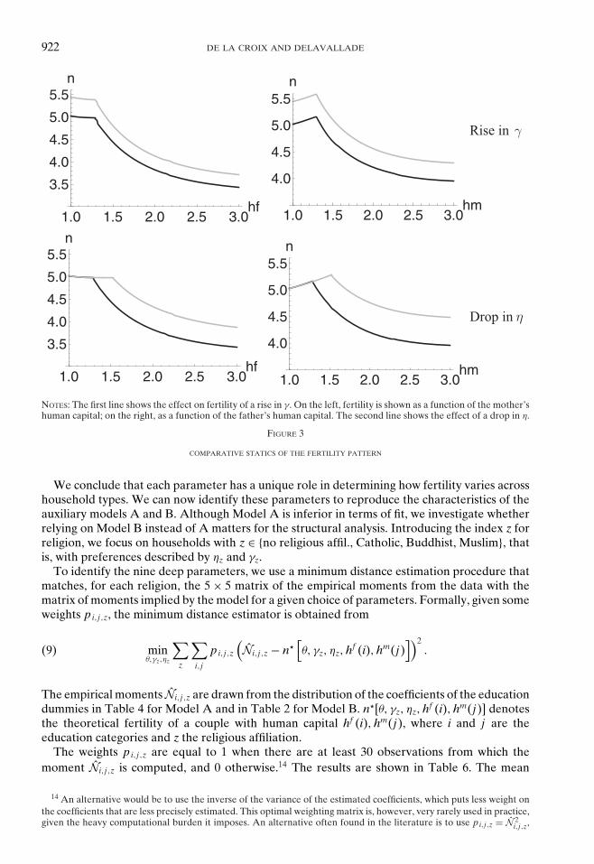
Three parameters remain to be identified: θ, γ, and η. We assume that θ is common to allreligions. To verify that these parameters can be identified through the fertility pattern describedin Equation (8), we draw the shift in the fertility function implied by a change in each of theparameters. Figure 3 reports the results, with, in the left column, fertility as a function of thehuman capital of a mother married to a man with no education, and, in the right column,fertility as a function of the human capital of a father married to a woman with no education.The left panel of each figure depicts the corner regime with no education. Entering the interiorregime, fertility drops as the quality–quantity trade-off kicks in. As parents’ education increases,spending on quality (education) substitutes to spending on quantity.
The preference for children γ acts as a shift on the whole pattern, affecting fertility in the sameway in both the corner regime and the interior regime. The parameter η acts on the point wherethe regime shifts. It also affects the speed at which fertility declines as the parents’ educationrises. The existence of the corner regime is critical for identification. In the absence of such aregime, fertility would be monotonically decreasing in education, and both η and γ would shiftthe whole pattern in the same way. The existence of different regimes of fertility is stronglyconfirmed by the literature on fertility differentials in developing countries. Jejeebhoy (1995)finds a positive or no relationship for seven countries, a negative relationship for 26 countries,and an inverse U-shaped relationship for 26 other countries. More recently, Vogl (2016) findsevidence of a relationship ranging over time from positive to negative.
13 Note that, in the theory, we have abstracted from different rates of return for boys and girls. If ξ was differentacross genders, it would be optimal to differentiate the education of boys and girls, investing more in the human capitalwith the highest return. One would then need to consider fertility as a sequential choice, in which the total number ofchildren would depend on whether parents had boys or girls in the first place. See Hazan and Zoabi (2015).
922 DE LA CROIX AND DELAVALLADE
1.0 1.5 2.0 2.5 3.0hf
3.5
4.0
4.5
5.0
5.5n
1.0 1.5 2.0 2.5 3.0hm
4.0
4.5
5.0
5.5n
1.0 1.5 2.0 2.5 3.0
Rise in
hm
4.0
4.5
5.0
5.5n
1.0 1.5 2.0 2.5 3.0hf
3.5
4.0
4.5
5.0
5.5n
Drop in
NOTES: The first line shows the effect on fertility of a rise in γ. On the left, fertility is shown as a function of the mother’shuman capital; on the right, as a function of the father’s human capital. The second line shows the effect of a drop in η.
FIGURE 3
COMPARATIVE STATICS OF THE FERTILITY PATTERN
We conclude that each parameter has a unique role in determining how fertility varies acrosshousehold types. We can now identify these parameters to reproduce the characteristics of theauxiliary models A and B. Although Model A is inferior in terms of fit, we investigate whetherrelying on Model B instead of A matters for the structural analysis. Introducing the index z forreligion, we focus on households with z ∈ {no religious affil., Catholic, Buddhist, Muslim}, thatis, with preferences described by ηz and γz.
To identify the nine deep parameters, we use a minimum distance estimation procedure thatmatches, for each religion, the 5 × 5 matrix of the empirical moments from the data with thematrix of moments implied by the model for a given choice of parameters. Formally, given someweights pi,j,z, the minimum distance estimator is obtained from
minθ,γz,ηz
∑z
∑i,j
pi,j,z
(Ni,j,z − n�
[θ, γz, ηz, hf (i), hm(j)
])2.(9)
The empirical moments Ni,j,z are drawn from the distribution of the coefficients of the educationdummies in Table 4 for Model A and in Table 2 for Model B. n�[θ, γz, ηz, hf (i), hm(j)] denotesthe theoretical fertility of a couple with human capital hf (i), hm(j), where i and j are theeducation categories and z the religious affiliation.
The weights pi,j,z are equal to 1 when there are at least 30 observations from which themoment Ni,j,z is computed, and 0 otherwise.14 The results are shown in Table 6. The mean
14 An alternative would be to use the inverse of the variance of the estimated coefficients, which puts less weight onthe coefficients that are less precisely estimated. This optimal weighting matrix is, however, very rarely used in practice,given the heavy computational burden it imposes. An alternative often found in the literature is to use pi,j,z = N 2
i,j,z,
RELIGIONS, FERTILITY, AND GROWTH 923
TABLE 6ESTIMATION OF THE DEEP PARAMETERS WITH (9)
Model A Model B
No Religion Catholic Buddhist Muslim No Religion Catholic Buddhist Muslim
θ 0.050 0.055(0.0035) (0.0012)
γz 0.553 0.717 0.607 0.649 0.672 0.746 0.612 0.703(0.0227) (0.0225) (0.0215) (0.0224) (0.0360) (0.0114) (0.0156) (0.0088)
ηz 1.802 1.737 1.759 1.748 2.136 1.943 1.862 1.746(0.0877) (0.0853) (0.0900) (0.0898) (0.0535) (0.0325) (0.0350) (0.0541)
NOTE: Mean (SD) of structural parameters minimizing Function (9), for 200 draws of the fertility matrices Ni,j,z.
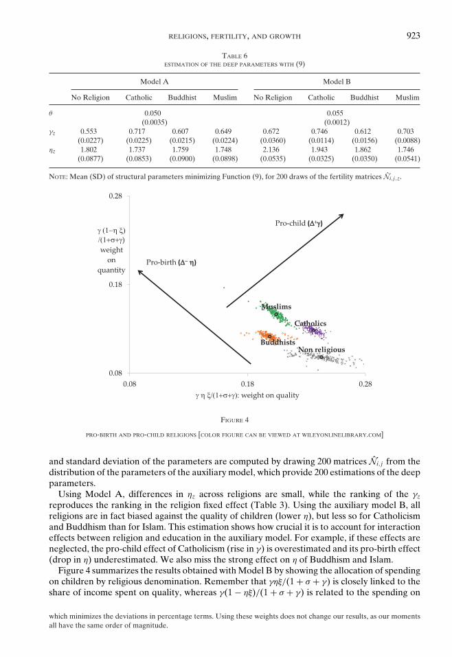
FIGURE 4
PRO-BIRTH AND PRO-CHILD RELIGIONS [COLOR FIGURE CAN BE VIEWED AT WILEYONLINELIBRARY.COM]
and standard deviation of the parameters are computed by drawing 200 matrices Ni,j from thedistribution of the parameters of the auxiliary model, which provide 200 estimations of the deepparameters.
Using Model A, differences in ηz across religions are small, while the ranking of the γz
reproduces the ranking in the religion fixed effect (Table 3). Using the auxiliary model B, allreligions are in fact biased against the quality of children (lower η), but less so for Catholicismand Buddhism than for Islam. This estimation shows how crucial it is to account for interactioneffects between religion and education in the auxiliary model. For example, if these effects areneglected, the pro-child effect of Catholicism (rise in γ) is overestimated and its pro-birth effect(drop in η) underestimated. We also miss the strong effect on η of Buddhism and Islam.
Figure 4 summarizes the results obtained with Model B by showing the allocation of spendingon children by religious denomination. Remember that γηξ/(1 + σ + γ) is closely linked to theshare of income spent on quality, whereas γ(1 − ηξ)/(1 + σ + γ) is related to the spending on
which minimizes the deviations in percentage terms. Using these weights does not change our results, as our momentsall have the same order of magnitude.

924 DE LA CROIX AND DELAVALLADE
quantity. These are the two dimensions plotted on the graph. The line with a negative slope isan iso-γ line. Moving to the North-East means that γ increases, as well as the total spendingon children and the pro-child dimension of the considered religion. Moving to the North-Westmeans that η decreases for a given γ and the considered religion is more pro-birth, directingspending toward quantity.
For each religion, we plot the estimated deep parameters for 200 draws of the parameters ofthe auxiliary model. This gives a sense of the uncertainty surrounding the estimates. We alsoplot the mean estimation as a circle.
Let us finally comment on the value of θ. Importantly, parameter θ determines the thresholdat which parents shift from no spending on the quality of children to facing a trade-off betweenquantity and quality of children (Equation (6)). To understand the implications of a θ estimatedaround 0.05, let us consider a couple with a husband and wife who have the same human capitalht. Equation (6) can be rewritten as (for a couple with no religion):
h >θ
2√
ωφηξhT = 0.055
2√
0.75 0.065 × 2.136 × 0.333hT = 0.69hT.
Hence, only couples with human capital at least equal to 69% of the human capital of theteacher (whom we assumed to be at the secondary school level) will invest in education andlower their fertility. If θ was zero, all couples would invest in education.
4. RELIGIONS AND GROWTH
We now embed the household model described above into a simple growth model. Theobjective is to infer some dynamic, long-run implications for growth, fertility, and education.We however refrain from any statement on welfare effects, as it would involve comparingindividuals with different preferences (induced by religion). We first develop the model, thensimulate the path of hypothetical countries populated by homogeneous religious groups tounderstand the specificities of each of them, and finally simulate the growth rates of realcountries with the religious composition observed in the data.
4.1. Theory. To simplify, and to abstract from any role played by inequality, we considerthe case of an economy composed of individuals with the same human capital ht = hm
t = hft and
of teachers with human capital hT, whose demographic weight in the population is negligible.15
The efficiency parameter μt in the human capital accumulation Equation (5) is assumed tofollow
μt = μhκt (1 + ρ)(1−κ)t,(10)
where human capital ht is a geometric average of the parents’ and the teacher’s human capital:
ht = hτt hT1−τ
.
The parameter τ captures the intergenerational transmission of ability and human capital for-mation within the family that does not go through formal schooling. Empirical studies detectsuch effects, but they are relatively small.
As in Rangazas (2000), Equation (10) is compatible with endogenous growth for κ = 1 andwith exogenous growth otherwise.
� When κ = 1, μt depends linearly on aggregate human capital. This is the simplest way ofmodeling a human capital externality driving the growth process. The empirical evidence
15 When there are no idiosyncratic ability shocks, the model of de la Croix and Doepke (2003) converges to a situationin which inequality vanishes asymptotically.

RELIGIONS, FERTILITY, AND GROWTH 925
supporting the fact that education is one of the key determinants of growth is strong, bothin terms of the quantity of education (Cohen and Soto, 2007) and the quality of education(Hanushek and Woessmann, 2012). This is a case in which a change in parameters drivinghuman capital accumulation will have the strongest effect on income per person, as thegrowth rate itself will be modified. Thus, it gives an upper bound on the pro-child effecton growth.
� Conversely, when κ < 1, growth is exogenous, and changes in parameters will only leadto differences in the levels of income per person. Parameter κ could be interpreted as ameasure of human capital externalities. Existing evidence (see Acemoglu and Angrist,2001; Krueger and Lindahl, 2001) suggests that these externalities are small, that is, thesocial return on human capital accumulation is only slightly larger than the private return.The standard model of exogenous growth is obtained when κ = 0.
The production of the final good is carried out by a single representative firm that operatesthe technology:
Yt = AKεt L1−ε
t ,
where Kt is aggregate capital, Lt is aggregate labor input in efficiency units, A > 0, and ε ∈ (0, 1).Physical capital completely depreciates in one period. The firm chooses inputs by maximizingprofits Yt − wtLt − RtKt. As a consequence, factor prices are
wt = (1 − ε)AKεt L−ε
t , and Rt = εAKε−1t L1−ε
t .
The adult population, measured by the number of couples Pt+1, is given by
Pt+1 = Pt(nt/2).(11)
The market-clearing conditions for capital are
Kt+1 = Ptst.(12)
The time spent rearing children follows:
aft = φn/
√ω, am
t = φn√
ω.
The market-clearing conditions for labor are
Lt = [ωht(1 − φn/
√ω) + ht(1 − φn
√ω) − etnthT]
Pt.(13)
This last condition reflects the fact that the time devoted to teaching is not available for goodsproduction.
When the human capital of the population ht is small compared to that of the teachers hT
(from Equation (6)), the economy is in a corner regime.
PROPOSITION 1 (CORNER REGIME). In the corner regime, a pro-child religion (�+γ) has a neg-ative effect on income per capita. A pro-birth religion (�−η) has no effect beyond making thecorner regime more likely.
PROOF. see Appendix A.2.
Many authors see the development process as initially driven by physical capital accumulation.Later on, “the process of industrialization was characterized by a gradual increase in the relative
926 DE LA CROIX AND DELAVALLADE
importance of human capital for the production process” (see Galor and Moav, 2006). In oursimple setup, this corresponds to crossing the threshold xt > θhT
φηξ. In the interior regime, human
capital is endogenous as et > 0. The economy converges16 toward a balanced growth path(BGP), which is characterized by the following proposition.
PROPOSITION 2 (GROWTH ALONG THE BGP). If
2ηφξ√
ω > θ(14)
the long-run growth factor of GDP per capita is
g = μ
(θ + 2ηφξ
√ω − θ
1 − ηξ
)if κ = 1 and g = 1 + ρ otherwise.A pro-child religion (�+γ) has no effect on long-run growth. A pro-birth religion (�−η) per-
manently affects the long-run growth rate in the endogenous growth case (κ = 1).
PROOF. see Appendix A.2.
PROPOSITION 3 (INCOME PER PERSON ALONG THE BGP). When growth is exogenous (κ < 1):A pro-child religion (�+γ) lowers the long-run income per person y through physical capital
accumulation k. A pro-birth religion (�−η) lowers the long-run income per person y throughhuman capital accumulation h.
PROOF. see Appendix A.2.
4.2. Calibration and Simulation of Religion-Specific Effects. To simulate the effect of reli-gious composition on growth, we retain the individual-specific parameters identified in theprevious section from Model B. In addition, we need to calibrate the macroeconomic parame-ters τ, κ, ρ, ε, μ, and A. τ is set to 0.1, in line with the evidence in Leibowitz (1974), who finds thateven after controlling for parents’ schooling and education, a 10% increase in parental incomeincreases a child’s future earnings by up to 0.85%. κ will be either 0 or 1, depending on theassumed model (exogenous or endogenous growth, respectively). The remaining parametersare chosen so as to match a hypothetical balanced growth path similar to the one achieved bydeveloped countries in the post-war period (see, e.g., Lagerlof, 2006). ρ is set so as to have agrowth rate of income per capita of 2% per year in the exogenous growth model. The shareof capital in added value is set to its usual value ε = 1/3. We calibrate the constant μ so asto reproduce a long-run growth rate g of 2% per year in a country whose entire population iswithout religious affiliation. Using the value of the growth rate along the BGP leads to μ = 3.46with κ = 1 and μ = 1.91 with κ = 0. As a normalization, we set the value of the scale parameterA in the production function to obtain a wage equal to 1 in the long run. It yields A = 3.4.
We first consider the exogenous growth version of the model. We accordingly set κ = 0and simulate a dynamic path for a hypothetical economy composed of individuals with noreligious affiliation. The initial conditions are such that hT = 1, ht = 0.3, and capital is such thatthe capital labor ratio takes its steady-state value. Starting from the same initial conditions,we do the same for a hypothetical economy composed of Catholics, Buddhists, and Muslims.Key macroeconomic variables after one period (t = 1) and six periods (t = 6) are presented inTable 7.
In period 1, fertility is high everywhere, but more so in the Catholic and Muslim artificialeconomies. The economies are not far from the corner regime, and households’ educational
16 Provided that some stability condition is met. ξη + τ < 1 suffices. See de la Croix and Doepke (2003).
RELIGIONS, FERTILITY, AND GROWTH 927
TABLE 7MACROECONOMIC VARIABLES AFTER 1 AND 6 PERIODS (κ = 0)
Value in Each of the Four Hypothetical Economies
Period Variable No Religious Affiliation Catholics Buddhists Muslims
t = 1 nt 4.62 5.07 4.56 5.10θ + et (% GDP) 10.19% 10.10% 8.48% 8.37%st/((1 + ω)htwt) 15.17% 14.64% 15.59% 14.94%Lt/(Ptht) 1.17 1.13 1.19 1.14yt 0.95 0.89 0.98 0.92annual growth 2.03% 1.91% 2.09% 1.95%
t = 6 nt 3.16 4.01 3.77 4.49θ + et (% GDP) 14.01% 11.34% 8.15% 6.67%st/((1 + ω)htwt) 15.17% 14.64% 15.59% 14.94%Lt/(Ptht) 1.17 1.12 1.19 1.14yt 29.21 23.74 25.52 21.56annual growth 2.22% 2.13% 2.11% 2.07%
TABLE 8MACROECONOMIC VARIABLES AFTER 1 AND 6 PERIODS (κ = 1)
Value in Each of the Four Hypothetical Economies
Period Variable No Religious Affiliation Catholics Buddhists Muslims
t = 1 nt 5.31 5.67 5.03 5.46θ + et (% GDP) 4.26% 4.49% 4.08% 4.35%yt 1.28 1.22 1.34 1.25annual growth 3.06% 2.97% 3.15% 3.02%
t = 6 nt 3.93 4.40 4.04 4.69θ + et (% GDP) 8.91% 8.68% 6.42% 5.44%yt 39.87 23.77 22.54 15.38annual growth 2.24% 1.85% 1.71% 1.48%
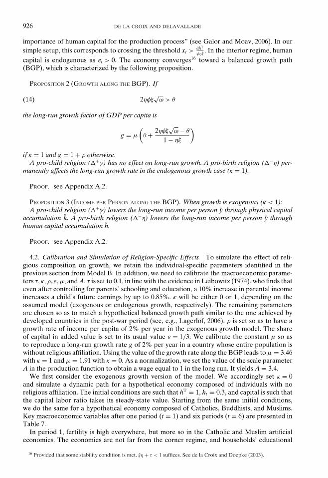
spending, et, is small. Considering θ as exogenous (possibly public) educational spending, theshare of this spending in GDP is between 8% and 10%. Saving over maximum income is around15%. The lowest saving rate is seen in the Catholic country, as it is the most pro-child religion(high γ). The labor supply is also lower in this economy, as having children takes time. Thelevel of income per person, yt, is smaller in the Catholic country for these two reasons. Thesimulation shows that the effect is, however, relatively small quantitatively.
In period 6, all economies are now well into the interior regime. Fertility has fallen comparedto period 1 and is now clearly higher in the Muslim country. This arises because the pro-birthdimension of religions now matters in the interior regime, and Islam is estimated to be the mostpro-birth (lower η). The ranking of parameter η is reflected in the share of education spendingin GDP, which ranges from 14.01% in the country with no religious affiliation to 6.67% inthe Muslim country. The saving rate is the same as in period 1 (this is a consequence of thelogarithmic utility function), whereas the labor supply has not changed much. The gap in GDPis now wider, as it results from accumulated discrepancies. In terms of growth rate, the pro-birthdimension of the different religions leads them to lose from 0.09% to 0.15% points of growthper year.
Next, we consider the endogenous growth version of the model, which will give us an upperbound on the long-run effect of religions on growth and income levels. We accordingly set κ = 1.Key macroeconomic variables after one period (t = 1) and six periods (t = 6) are presented inTable 8. We do not report the saving rate and labor supply, as they are virtually identical to thosein Table 7. In period 1, households are in the corner regime, and their educational spending et
928 DE LA CROIX AND DELAVALLADE
0
10
20
30
40
50
60
Nonreligious
Catholics Buddhists Muslims Nonreligious
Catholics Buddhists Muslims
Endogenous growth Exogenous growth
FIGURE 5
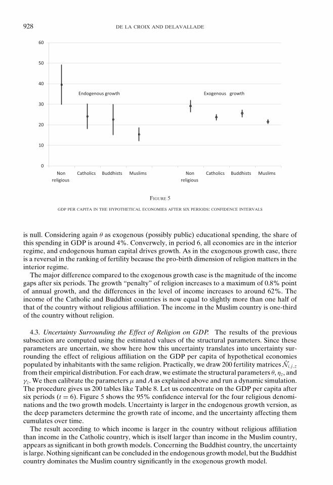
GDP PER CAPITA IN THE HYPOTHETICAL ECONOMIES AFTER SIX PERIODS: CONFIDENCE INTERVALS
is null. Considering again θ as exogenous (possibly public) educational spending, the share ofthis spending in GDP is around 4%. Converwely, in period 6, all economies are in the interiorregime, and endogenous human capital drives growth. As in the exogenous growth case, thereis a reversal in the ranking of fertility because the pro-birth dimension of religion matters in theinterior regime.
The major difference compared to the exogenous growth case is the magnitude of the incomegaps after six periods. The growth “penalty” of religion increases to a maximum of 0.8% pointof annual growth, and the differences in the level of income increases to around 62%. Theincome of the Catholic and Buddhist countries is now equal to slightly more than one half ofthat of the country without religious affiliation. The income in the Muslim country is one-thirdof the country without religion.
4.3. Uncertainty Surrounding the Effect of Religion on GDP. The results of the previoussubsection are computed using the estimated values of the structural parameters. Since theseparameters are uncertain, we show here how this uncertainty translates into uncertainty sur-rounding the effect of religious affiliation on the GDP per capita of hypothetical economiespopulated by inhabitants with the same religion. Practically, we draw 200 fertility matrices Ni,j,z
from their empirical distribution. For each draw, we estimate the structural parameters θ, ηz, andγz. We then calibrate the parameters μ and A as explained above and run a dynamic simulation.The procedure gives us 200 tables like Table 8. Let us concentrate on the GDP per capita aftersix periods (t = 6). Figure 5 shows the 95% confidence interval for the four religious denomi-nations and the two growth models. Uncertainty is larger in the endogenous growth version, asthe deep parameters determine the growth rate of income, and the uncertainty affecting themcumulates over time.
The result according to which income is larger in the country without religious affiliationthan income in the Catholic country, which is itself larger than income in the Muslim country,appears as significant in both growth models. Concerning the Buddhist country, the uncertaintyis large. Nothing significant can be concluded in the endogenous growth model, but the Buddhistcountry dominates the Muslim country significantly in the exogenous growth model.
RELIGIONS, FERTILITY, AND GROWTH 929
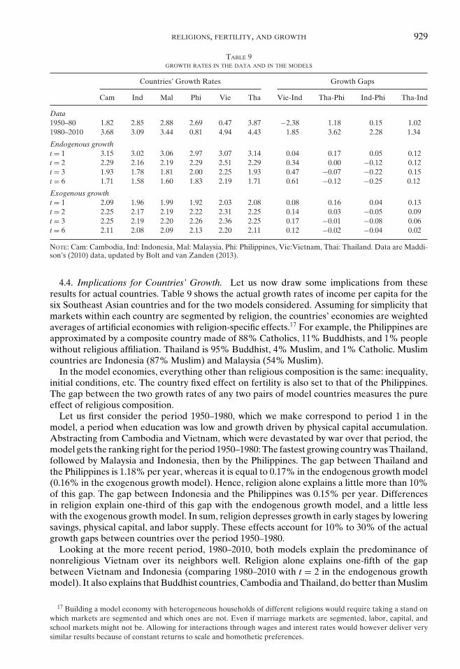
TABLE 9GROWTH RATES IN THE DATA AND IN THE MODELS
Countries’ Growth Rates Growth Gaps
Cam Ind Mal Phi Vie Tha Vie-Ind Tha-Phi Ind-Phi Tha-Ind
Data1950–80 1.82 2.85 2.88 2.69 0.47 3.87 −2.38 1.18 0.15 1.021980–2010 3.68 3.09 3.44 0.81 4.94 4.43 1.85 3.62 2.28 1.34
Endogenous growtht = 1 3.15 3.02 3.06 2.97 3.07 3.14 0.04 0.17 0.05 0.12t = 2 2.29 2.16 2.19 2.29 2.51 2.29 0.34 0.00 −0.12 0.12t = 3 1.93 1.78 1.81 2.00 2.25 1.93 0.47 −0.07 −0.22 0.15t = 6 1.71 1.58 1.60 1.83 2.19 1.71 0.61 −0.12 −0.25 0.12
Exogenous growtht = 1 2.09 1.96 1.99 1.92 2.03 2.08 0.08 0.16 0.04 0.13t = 2 2.25 2.17 2.19 2.22 2.31 2.25 0.14 0.03 −0.05 0.09t = 3 2.25 2.19 2.20 2.26 2.36 2.25 0.17 −0.01 −0.08 0.06t = 6 2.11 2.08 2.09 2.13 2.20 2.11 0.12 −0.02 −0.04 0.02
NOTE: Cam: Cambodia, Ind: Indonesia, Mal: Malaysia, Phi: Philippines, Vie:Vietnam, Thai: Thailand. Data are Maddi-son’s (2010) data, updated by Bolt and van Zanden (2013).
4.4. Implications for Countries’ Growth. Let us now draw some implications from theseresults for actual countries. Table 9 shows the actual growth rates of income per capita for thesix Southeast Asian countries and for the two models considered. Assuming for simplicity thatmarkets within each country are segmented by religion, the countries’ economies are weightedaverages of artificial economies with religion-specific effects.17 For example, the Philippines areapproximated by a composite country made of 88% Catholics, 11% Buddhists, and 1% peoplewithout religious affiliation. Thailand is 95% Buddhist, 4% Muslim, and 1% Catholic. Muslimcountries are Indonesia (87% Muslim) and Malaysia (54% Muslim).
In the model economies, everything other than religious composition is the same: inequality,initial conditions, etc. The country fixed effect on fertility is also set to that of the Philippines.The gap between the two growth rates of any two pairs of model countries measures the pureeffect of religious composition.
Let us first consider the period 1950–1980, which we make correspond to period 1 in themodel, a period when education was low and growth driven by physical capital accumulation.Abstracting from Cambodia and Vietnam, which were devastated by war over that period, themodel gets the ranking right for the period 1950–1980: The fastest growing country was Thailand,followed by Malaysia and Indonesia, then by the Philippines. The gap between Thailand andthe Philippines is 1.18% per year, whereas it is equal to 0.17% in the endogenous growth model(0.16% in the exogenous growth model). Hence, religion alone explains a little more than 10%of this gap. The gap between Indonesia and the Philippines was 0.15% per year. Differencesin religion explain one-third of this gap with the endogenous growth model, and a little lesswith the exogenous growth model. In sum, religion depresses growth in early stages by loweringsavings, physical capital, and labor supply. These effects account for 10% to 30% of the actualgrowth gaps between countries over the period 1950–1980.
Looking at the more recent period, 1980–2010, both models explain the predominance ofnonreligious Vietnam over its neighbors well. Religion alone explains one-fifth of the gapbetween Vietnam and Indonesia (comparing 1980–2010 with t = 2 in the endogenous growthmodel). It also explains that Buddhist countries, Cambodia and Thailand, do better than Muslim
17 Building a model economy with heterogeneous households of different religions would require taking a stand onwhich markets are segmented and which ones are not. Even if marriage markets are segmented, labor, capital, andschool markets might not be. Allowing for interactions through wages and interest rates would however deliver verysimilar results because of constant returns to scale and homothetic preferences.

930 DE LA CROIX AND DELAVALLADE
countries. Religion explains 13% of the gap between Thailand and Indonesia, for example.There is, however, one feature of the data that we cannot explain by religion. In the endogenousgrowth model, the Philippines should do well because Catholics are relatively pro-child, andeducation is not neglected. This is obviously not the case in the data.18
In sum, in the later stages of growth, pro-birth religions lower the growth and human capitalaccumulation, explaining between 10% and 20% of the gap between Muslim and Buddhistcountries in Southeast Asia over the period 1980–2010. The low performance of the Philippinesremains, however, unexplained.
An interesting implication we can draw for actual countries is inferred from the artificialperiod 6. Here, the two countries with a large Muslim population, Indonesia and Malaysia, areexpected to suffer from a lack of investment in human capital. According to the endogenoushuman capital model, Indonesia (87% Muslim) and Malaysia (54% Muslim) would grow at1.58% and 1.60%, respectively, whereas the Philippines and Thailand would grow at 1.83% and1.71%, respectively.
Two remarks are in order before we turn to the robustness analysis. First, the use of anendogenous growth model in which human capital is the engine of growth is in accordance withthe recent empirical literature on education and growth, but obviously gives a central role to thequality–quantity trade-off. If endogenous growth were driven by physical capital accumulationinstead, such as in the AK model, the religion that discourages saving the most would havehad the most dramatic effects on growth. Second, our estimated effects rely upon the fertilitybehavior of women in Southeast Asia, born between 1900 and 1963. During that time, one mightthink that there was a strong link between religious precepts and behavior. Using these resultsto forecast future trends would be far-fetched, as this link may become looser with the rise ofsecularization.
5. ROBUSTNESS ANALYSIS
In this section, we analyze the robustness of the results to various assumptions we madealong the way of the identification process. For each analysis, we reproduce Figures 4 and 5with the new estimates; this allows us to assess whether the characterization of religions inthe pro-child/pro-birth dimension is amended and whether the consequences for growth arealtered.
5.1. Higher Returns to Schooling. First, instead of estimating the human capital by educationlevels in Table 5 from a single study on the Philippines (which fitted our needs well, as it usedthe same education categories as IPUMS), we average the recent estimates of Mincer regres-sion coefficients provided in Montenegro and Patrinos (2014; presented in Appendix A.4.1)over Southeast Asian countries. Taking these returns makes a big difference. The income gapbetween low and highly educated people is now much larger.
The structural parameters are estimated with these new levels of human capital, keepingall other assumptions unchanged. From Appendix A.4.1, we see that parameter θ, which iskey in determining the human capital threshold below which households do not invest ineducation (Equation (6)), is halved compared to the benchmark estimation; this adjustmentof θ ensures that households with primary education, which are now much poorer, relatively,because of the higher returns to schooling, are kept in the interior regime. Parameters ηz arealso revised downward. The left panel of Figure 6, to be compared to Figure 4, shows that therelative characteristics of each religion are not altered by the higher returns to schooling. Islamremains the most pro-birth religion, and Catholicism the most pro-child. The results in termsof macroeconomic outcomes are presented in the right panel of Figure 6, to be compared withFigure 5 in the benchmark. The ranking in terms of growth of the various hypothetical countries
18 In his famous article, Lucas (1993) already stressed that the Philippines and South Korea started from similar initialconditions in 1950, but ended up growing at very different rates.
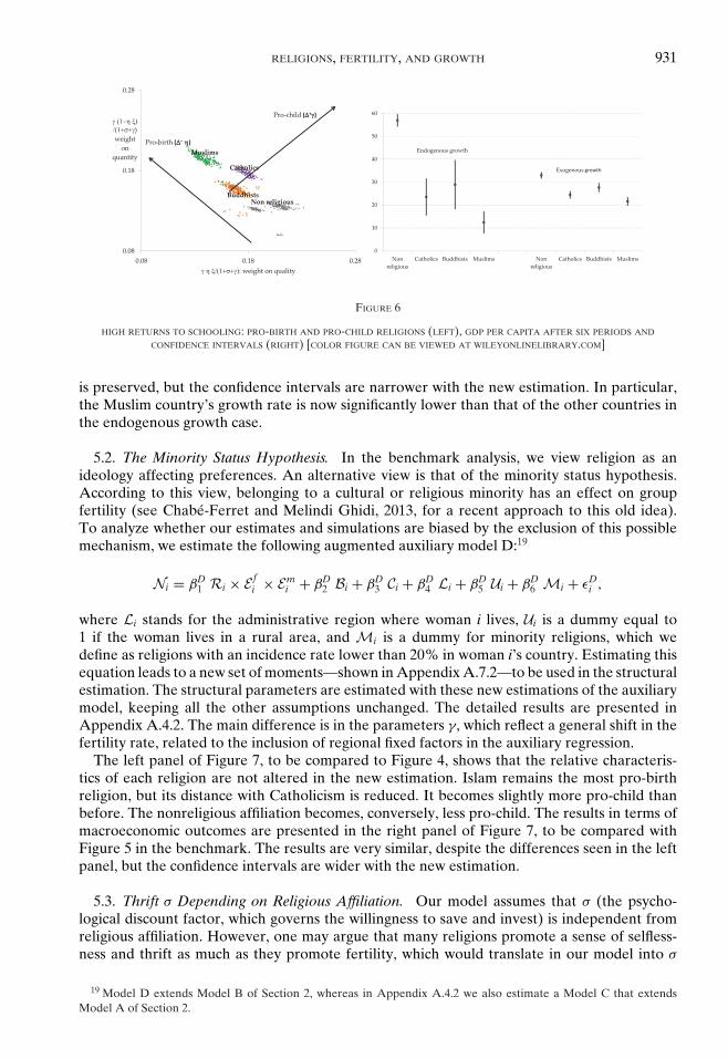
RELIGIONS, FERTILITY, AND GROWTH 931
FIGURE 6
HIGH RETURNS TO SCHOOLING: PRO-BIRTH AND PRO-CHILD RELIGIONS (LEFT), GDP PER CAPITA AFTER SIX PERIODS AND
CONFIDENCE INTERVALS (RIGHT) [COLOR FIGURE CAN BE VIEWED AT WILEYONLINELIBRARY.COM]
is preserved, but the confidence intervals are narrower with the new estimation. In particular,the Muslim country’s growth rate is now significantly lower than that of the other countries inthe endogenous growth case.
5.2. The Minority Status Hypothesis. In the benchmark analysis, we view religion as anideology affecting preferences. An alternative view is that of the minority status hypothesis.According to this view, belonging to a cultural or religious minority has an effect on groupfertility (see Chabe-Ferret and Melindi Ghidi, 2013, for a recent approach to this old idea).To analyze whether our estimates and simulations are biased by the exclusion of this possiblemechanism, we estimate the following augmented auxiliary model D:19
Ni = βD1 Ri × E f
i × Emi + βD
2 Bi + βD3 Ci + βD
4 Li + βD5 Ui + βD
6 Mi + εDi ,
where Li stands for the administrative region where woman i lives, Ui is a dummy equal to1 if the woman lives in a rural area, and Mi is a dummy for minority religions, which wedefine as religions with an incidence rate lower than 20% in woman i’s country. Estimating thisequation leads to a new set of moments—shown in Appendix A.7.2—to be used in the structuralestimation. The structural parameters are estimated with these new estimations of the auxiliarymodel, keeping all the other assumptions unchanged. The detailed results are presented inAppendix A.4.2. The main difference is in the parameters γ, which reflect a general shift in thefertility rate, related to the inclusion of regional fixed factors in the auxiliary regression.
The left panel of Figure 7, to be compared to Figure 4, shows that the relative characteris-tics of each religion are not altered in the new estimation. Islam remains the most pro-birthreligion, but its distance with Catholicism is reduced. It becomes slightly more pro-child thanbefore. The nonreligious affiliation becomes, conversely, less pro-child. The results in terms ofmacroeconomic outcomes are presented in the right panel of Figure 7, to be compared withFigure 5 in the benchmark. The results are very similar, despite the differences seen in the leftpanel, but the confidence intervals are wider with the new estimation.
5.3. Thrift σ Depending on Religious Affiliation. Our model assumes that σ (the psycho-logical discount factor, which governs the willingness to save and invest) is independent fromreligious affiliation. However, one may argue that many religions promote a sense of selfless-ness and thrift as much as they promote fertility, which would translate in our model into σ
19 Model D extends Model B of Section 2, whereas in Appendix A.4.2 we also estimate a Model C that extendsModel A of Section 2.

932 DE LA CROIX AND DELAVALLADE
FIGURE 7
CONTROLLING FOR MINORITIES: PRO-BIRTH AND PRO-CHILD RELIGIONS (LEFT PANEL), GDP PER CAPITA AFTER SIX PERIODS AND
CONFIDENCE INTERVALS (RIGHT PANEL) [COLOR FIGURE CAN BE VIEWED AT WILEYONLINELIBRARY.COM]
depending on religious affiliation. The absence of data on savings makes it difficult to testthis alternative hypothesis. The only variable from the census that may be indicative concernswhether the respondent or her husband owns their house. Using house ownership as a proxyfor savings, we can estimate religion-specific σ using additional moment restrictions and analyzethe implications for our model and predictions.
We first estimate a new auxiliary regression in which house ownership is regressed on thesame variables as fertility (education level of husband and wife, religious affiliation, interactionterms, census, and birth fixed effects). This linear probability model allows us to construct themi,j,z, where i and j are education categories for wives and husbands, and z is their religiousaffiliation. The values are reported in Appendix A.7.3.
For the structural model, we relate average house ownership mi,j,z ∈ [0, 1] in each group{i, j, z} to savings through a logistic function with parameters δ0 and δ1:
mi,j,z = 11 + exp{δ1(si,j,z − δ0)} ,
and savings are given by Equation (A.3) from Appendix A.1:
st = σz
1 + σz + γz
(ωhf
i + hmj
).
These two equations give a theoretical house ownership rate m�[θ, γz, ηz, σz, hf (i), hm(j)], whichdepends on religion-specific thrift σz. The minimization problem of the structural estimationcan be written as
minθ,γz,ηz,σz,δ0,δ1
∑z
∑i,j
[pi,j,z
(Ni,j,z − n�
[θ, γz, ηz, σz, hf (i), hm(j)
])2
+pi,j,z
(mi,j,z − m�
[θ, γz, ηz, σz, hf (i), hm(j)
])2]
.(15)
Compared to Equation (9), we have additional parameters to estimate, δ0, δ1, and the σzs, andadditional moments to match, based on house ownership mi,j,z.
In the new estimation, presented in detail in Appendix A.4.3, the σzs are not significantlydifferent from the value we imposed a priori (0.3). They are estimated at 0.411 (nonreligious),
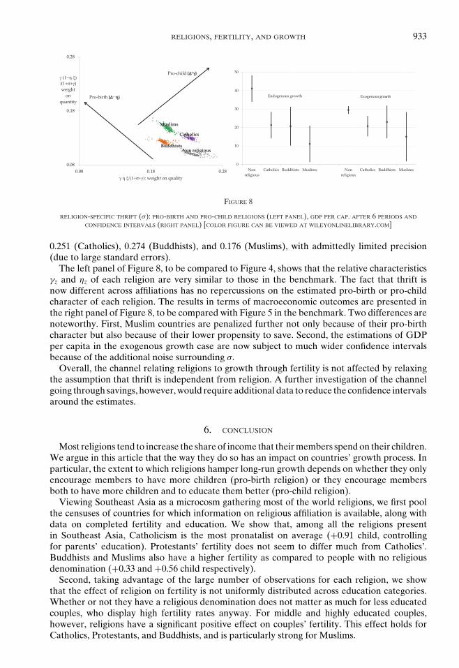
RELIGIONS, FERTILITY, AND GROWTH 933
FIGURE 8
RELIGION-SPECIFIC THRIFT (σ): PRO-BIRTH AND PRO-CHILD RELIGIONS (LEFT PANEL), GDP PER CAP. AFTER 6 PERIODS AND
CONFIDENCE INTERVALS (RIGHT PANEL) [COLOR FIGURE CAN BE VIEWED AT WILEYONLINELIBRARY.COM]
0.251 (Catholics), 0.274 (Buddhists), and 0.176 (Muslims), with admittedly limited precision(due to large standard errors).
The left panel of Figure 8, to be compared to Figure 4, shows that the relative characteristicsγz and ηz of each religion are very similar to those in the benchmark. The fact that thrift isnow different across affiliations has no repercussions on the estimated pro-birth or pro-childcharacter of each religion. The results in terms of macroeconomic outcomes are presented inthe right panel of Figure 8, to be compared with Figure 5 in the benchmark. Two differences arenoteworthy. First, Muslim countries are penalized further not only because of their pro-birthcharacter but also because of their lower propensity to save. Second, the estimations of GDPper capita in the exogenous growth case are now subject to much wider confidence intervalsbecause of the additional noise surrounding σ.
Overall, the channel relating religions to growth through fertility is not affected by relaxingthe assumption that thrift is independent from religion. A further investigation of the channelgoing through savings, however, would require additional data to reduce the confidence intervalsaround the estimates.
6. CONCLUSION
Most religions tend to increase the share of income that their members spend on their children.We argue in this article that the way they do so has an impact on countries’ growth process. Inparticular, the extent to which religions hamper long-run growth depends on whether they onlyencourage members to have more children (pro-birth religion) or they encourage membersboth to have more children and to educate them better (pro-child religion).
Viewing Southeast Asia as a microcosm gathering most of the world religions, we first poolthe censuses of countries for which information on religious affiliation is available, along withdata on completed fertility and education. We show that, among all the religions presentin Southeast Asia, Catholicism is the most pronatalist on average (+0.91 child, controllingfor parents’ education). Protestants’ fertility does not seem to differ much from Catholics’.Buddhists and Muslims also have a higher fertility as compared to people with no religiousdenomination (+0.33 and +0.56 child respectively).
Second, taking advantage of the large number of observations for each religion, we showthat the effect of religion on fertility is not uniformly distributed across education categories.Whether or not they have a religious denomination does not matter as much for less educatedcouples, who display high fertility rates anyway. For middle and highly educated couples,however, religions have a significant positive effect on couples’ fertility. This effect holds forCatholics, Protestants, and Buddhists, and is particularly strong for Muslims.
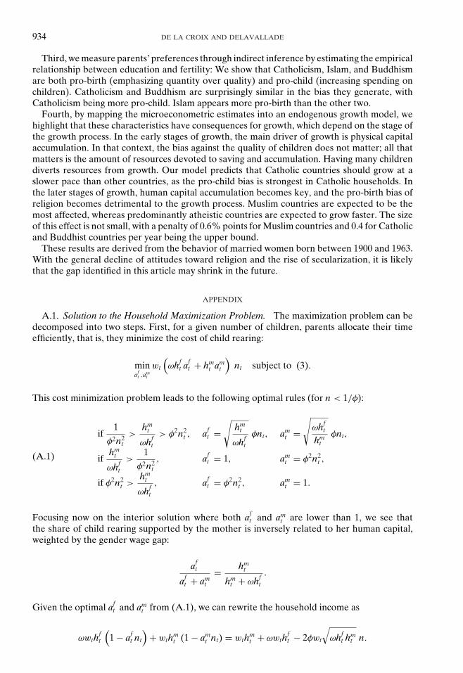
934 DE LA CROIX AND DELAVALLADE
Third, we measure parents’ preferences through indirect inference by estimating the empiricalrelationship between education and fertility: We show that Catholicism, Islam, and Buddhismare both pro-birth (emphasizing quantity over quality) and pro-child (increasing spending onchildren). Catholicism and Buddhism are surprisingly similar in the bias they generate, withCatholicism being more pro-child. Islam appears more pro-birth than the other two.
Fourth, by mapping the microeconometric estimates into an endogenous growth model, wehighlight that these characteristics have consequences for growth, which depend on the stage ofthe growth process. In the early stages of growth, the main driver of growth is physical capitalaccumulation. In that context, the bias against the quality of children does not matter; all thatmatters is the amount of resources devoted to saving and accumulation. Having many childrendiverts resources from growth. Our model predicts that Catholic countries should grow at aslower pace than other countries, as the pro-child bias is strongest in Catholic households. Inthe later stages of growth, human capital accumulation becomes key, and the pro-birth bias ofreligion becomes detrimental to the growth process. Muslim countries are expected to be themost affected, whereas predominantly atheistic countries are expected to grow faster. The sizeof this effect is not small, with a penalty of 0.6% points for Muslim countries and 0.4 for Catholicand Buddhist countries per year being the upper bound.
These results are derived from the behavior of married women born between 1900 and 1963.With the general decline of attitudes toward religion and the rise of secularization, it is likelythat the gap identified in this article may shrink in the future.
APPENDIX
A.1. Solution to the Household Maximization Problem. The maximization problem can bedecomposed into two steps. First, for a given number of children, parents allocate their timeefficiently, that is, they minimize the cost of child rearing:
minaf
t ,amt
wt
(ωhf
t aft + hm
t amt
)nt subject to (3).
This cost minimization problem leads to the following optimal rules (for n < 1/φ):
if1
φ2n2t
>hm
t
ωhft
> φ2n2t , af
t =√
hmt
ωhft
φnt, amt =
√ωhf
t
hmt
φnt,
ifhm
t
ωhft
>1
φ2n2t, af
t = 1, amt = φ2n2
t ,
if φ2n2t >
hmt
ωhft
, aft = φ2n2
t , amt = 1.
(A.1)
Focusing now on the interior solution where both aft and am
t are lower than 1, we see thatthe share of child rearing supported by the mother is inversely related to her human capital,weighted by the gender wage gap:
aft
aft + am
t
= hmt
hmt + ωhf
t
.
Given the optimal aft and am
t from (A.1), we can rewrite the household income as
ωwthft
(1 − af
t nt
)+ wthm
t (1 − amt nt) = wthm
t + ωwthft − 2φwt
√ωhf
t hmt n.
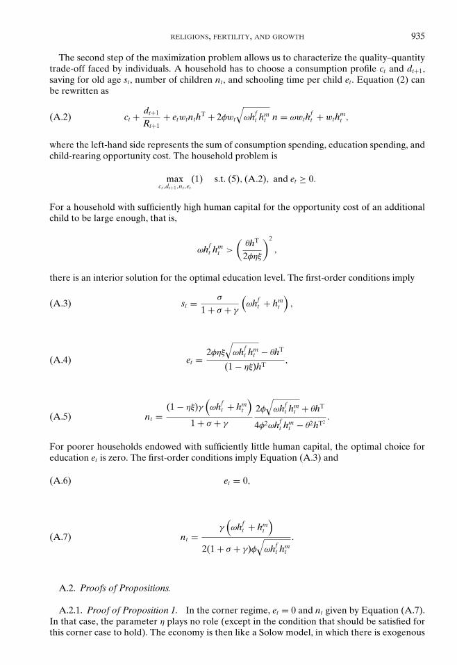
RELIGIONS, FERTILITY, AND GROWTH 935
The second step of the maximization problem allows us to characterize the quality–quantitytrade-off faced by individuals. A household has to choose a consumption profile ct and dt+1,saving for old age st, number of children nt, and schooling time per child et. Equation (2) canbe rewritten as
ct + dt+1
Rt+1+ etwtnthT + 2φwt
√ωhf
t hmt n = ωwth
ft + wthm
t ,(A.2)
where the left-hand side represents the sum of consumption spending, education spending, andchild-rearing opportunity cost. The household problem is
maxct,dt+1,nt,et
(1) s.t. (5), (A.2), and et ≥ 0.
For a household with sufficiently high human capital for the opportunity cost of an additionalchild to be large enough, that is,
ωhft hm
t >
(θhT
2φηξ
)2
,
there is an interior solution for the optimal education level. The first-order conditions imply
st = σ
1 + σ + γ
(ωhf
t + hmt
),(A.3)
et = 2φηξ
√ωhf
t hmt − θhT
(1 − ηξ)hT,(A.4)
nt =(1 − ηξ)γ
(ωhf
t + hmt
)1 + σ + γ
2φ
√ωhf
t hmt + θhT
4φ2ωhft hm
t − θ2hT2.(A.5)
For poorer households endowed with sufficiently little human capital, the optimal choice foreducation et is zero. The first-order conditions imply Equation (A.3) and
et = 0,(A.6)
nt =γ
(ωhf
t + hmt
)2(1 + σ + γ)φ
√ωhf
t hmt
.(A.7)
A.2. Proofs of Propositions.
A.2.1. Proof of Proposition 1. In the corner regime, et = 0 and nt given by Equation (A.7).In that case, the parameter η plays no role (except in the condition that should be satisfied forthis corner case to hold). The economy is then like a Solow model, in which there is exogenous

936 DE LA CROIX AND DELAVALLADE
technical progress (or exogenous human capital accumulation with κ = 1) driving growth andwhere physical capital accumulation is the key driver of dynamics.
The negative effect of increased γ on income goes through increased fertility byEquation (A.7), lower labor supply Lt by Equation (13), lower savings by Equation (A.3),and lower capital per person by Equation (12).
A.2.2. Proof of Proposition 2. Condition (14) ensures that the interior regime prevails inthe long run. Then, Equations (5), (A.4), and (10) imply the value of g in the proposition.
Comparative statics are then straightforward.
A.2.3. Proof of Proposition 3. Long-run variables in levels can be defined as
e = et = 2ηφξ√
ω − θ
1 − ηξ,
n = nt = (1 − ηξ)γ(1 + ω)1 + σ + γ
2φ√
ω + θ
4φ2ω − θ2,
h = ht
gt= (μ(θ + e)/g)
11−κ ,
s = st
gt= σ
1 + σ + γ(ω + 1)h,
� = Lt
Ptgt= [
ω(1 − φn/√
ω) + (1 − φn√
ω) − en]
h,
k = Kt
Pt(g)t= 2s
gn,
y = Yt
Pt(g)t= Akε�1−ε.
Computing how γ and η affect the above system, we infer the results in the proposition.
A.3. Descriptive Statistics: Subsample with Known Mother’s Religion.
Cambodia Indonesia Malaysia Philippines Vietnam Thailand
A: Number of children ever bornMean 3.65 3.79 5.00 2.88 3.23 2.55SD 2.47 3.09 2.82 2.40 1.58 1.98Min 0 0 0 0 0 0Max 13 14 9 11 12 12
B: Religion (in %)No religious affiliation 0 0 0 0 78.7 0Buddhist 99.1 1.4 33.3 0 15 98.3Hindu 0 0.9 5.6 0 0 0Muslim 0.6 89.4 33.3 0.9 0 1.7Catholic 0 2.3 5.6 90.7 3.9 0Protestant/other Christian 0 3.2 0 8.4 0.6 0Other 0.3 2.8 22.2 0 1.8 0
C:Women’s education (in %)No schooling 31.8 55.5 55.6 1.5 0.3 9.1Some primary 37.4 25 22.2 12.5 19.9 67.7
(Continued)
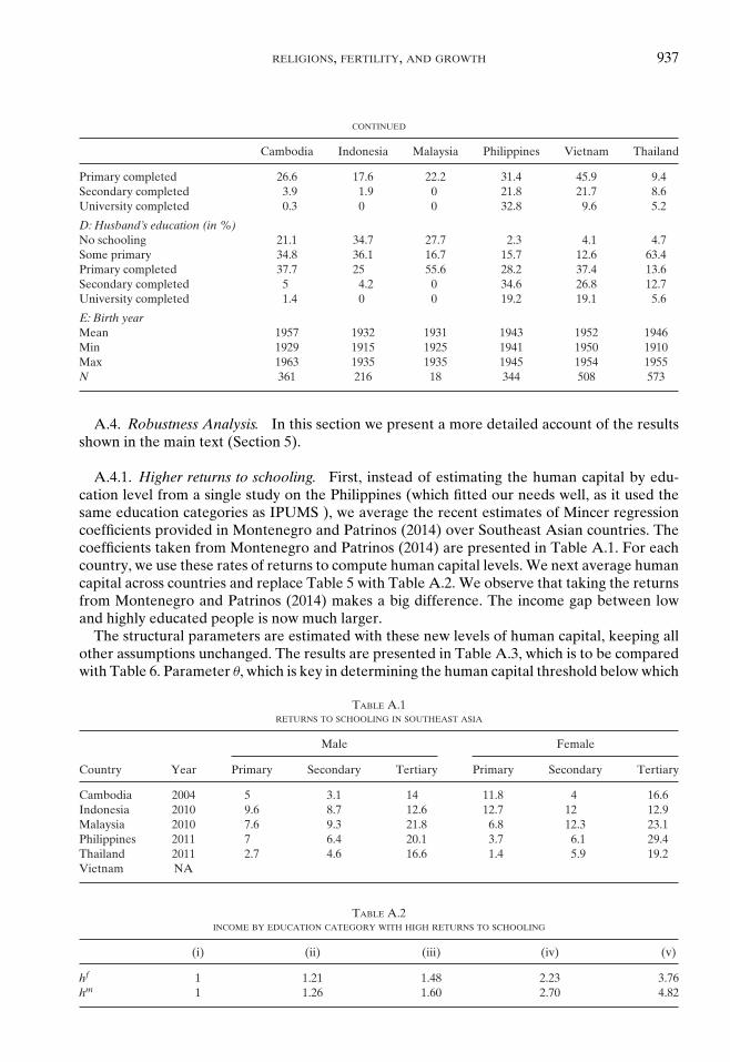
RELIGIONS, FERTILITY, AND GROWTH 937
CONTINUED
Cambodia Indonesia Malaysia Philippines Vietnam Thailand
Primary completed 26.6 17.6 22.2 31.4 45.9 9.4Secondary completed 3.9 1.9 0 21.8 21.7 8.6University completed 0.3 0 0 32.8 9.6 5.2
D:Husband’s education (in %)No schooling 21.1 34.7 27.7 2.3 4.1 4.7Some primary 34.8 36.1 16.7 15.7 12.6 63.4Primary completed 37.7 25 55.6 28.2 37.4 13.6Secondary completed 5 4.2 0 34.6 26.8 12.7University completed 1.4 0 0 19.2 19.1 5.6
E: Birth yearMean 1957 1932 1931 1943 1952 1946Min 1929 1915 1925 1941 1950 1910Max 1963 1935 1935 1945 1954 1955N 361 216 18 344 508 573
A.4. Robustness Analysis. In this section we present a more detailed account of the resultsshown in the main text (Section 5).
A.4.1. Higher returns to schooling. First, instead of estimating the human capital by edu-cation level from a single study on the Philippines (which fitted our needs well, as it used thesame education categories as IPUMS ), we average the recent estimates of Mincer regressioncoefficients provided in Montenegro and Patrinos (2014) over Southeast Asian countries. Thecoefficients taken from Montenegro and Patrinos (2014) are presented in Table A.1. For eachcountry, we use these rates of returns to compute human capital levels. We next average humancapital across countries and replace Table 5 with Table A.2. We observe that taking the returnsfrom Montenegro and Patrinos (2014) makes a big difference. The income gap between lowand highly educated people is now much larger.
The structural parameters are estimated with these new levels of human capital, keeping allother assumptions unchanged. The results are presented in Table A.3, which is to be comparedwith Table 6. Parameter θ, which is key in determining the human capital threshold below which
TABLE A.1RETURNS TO SCHOOLING IN SOUTHEAST ASIA
Male Female
Country Year Primary Secondary Tertiary Primary Secondary Tertiary
Cambodia 2004 5 3.1 14 11.8 4 16.6Indonesia 2010 9.6 8.7 12.6 12.7 12 12.9Malaysia 2010 7.6 9.3 21.8 6.8 12.3 23.1Philippines 2011 7 6.4 20.1 3.7 6.1 29.4Thailand 2011 2.7 4.6 16.6 1.4 5.9 19.2Vietnam NA
TABLE A.2INCOME BY EDUCATION CATEGORY WITH HIGH RETURNS TO SCHOOLING
(i) (ii) (iii) (iv) (v)
hf 1 1.21 1.48 2.23 3.76hm 1 1.26 1.60 2.70 4.82
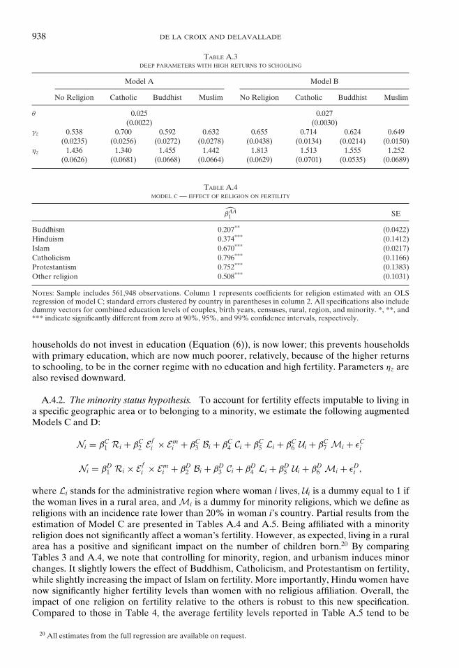
938 DE LA CROIX AND DELAVALLADE
TABLE A.3DEEP PARAMETERS WITH HIGH RETURNS TO SCHOOLING
Model A Model B
No Religion Catholic Buddhist Muslim No Religion Catholic Buddhist Muslim
θ 0.025 0.027(0.0022) (0.0030)
γz 0.538 0.700 0.592 0.632 0.655 0.714 0.624 0.649(0.0235) (0.0256) (0.0272) (0.0278) (0.0438) (0.0134) (0.0214) (0.0150)
ηz 1.436 1.340 1.455 1.442 1.813 1.513 1.555 1.252(0.0626) (0.0681) (0.0668) (0.0664) (0.0629) (0.0701) (0.0535) (0.0689)
TABLE A.4MODEL C — EFFECT OF RELIGION ON FERTILITY
βAA1 SE
Buddhism 0.207** (0.0422)Hinduism 0.374*** (0.1412)Islam 0.670*** (0.0217)Catholicism 0.796*** (0.1166)Protestantism 0.752*** (0.1383)Other religion 0.508*** (0.1031)
NOTES: Sample includes 561,948 observations. Column 1 represents coefficients for religion estimated with an OLSregression of model C; standard errors clustered by country in parentheses in column 2. All specifications also includedummy vectors for combined education levels of couples, birth years, censuses, rural, region, and minority. *, **, and*** indicate significantly different from zero at 90%, 95%, and 99% confidence intervals, respectively.
households do not invest in education (Equation (6)), is now lower; this prevents householdswith primary education, which are now much poorer, relatively, because of the higher returnsto schooling, to be in the corner regime with no education and high fertility. Parameters ηz arealso revised downward.
A.4.2. The minority status hypothesis. To account for fertility effects imputable to living ina specific geographic area or to belonging to a minority, we estimate the following augmentedModels C and D:
Ni = βC1 Ri + βC
2 E fi × Em
i + βC3 Bi + βC
4 Ci + βC5 Li + βC
6 Ui + βC7 Mi + εC
i
Ni = βD1 Ri × E f
i × Emi + βD
2 Bi + βD3 Ci + βD
4 Li + βD5 Ui + βD
6 Mi + εDi ,
where Li stands for the administrative region where woman i lives, Ui is a dummy equal to 1 ifthe woman lives in a rural area, and Mi is a dummy for minority religions, which we define asreligions with an incidence rate lower than 20% in woman i’s country. Partial results from theestimation of Model C are presented in Tables A.4 and A.5. Being affiliated with a minorityreligion does not significantly affect a woman’s fertility. However, as expected, living in a ruralarea has a positive and significant impact on the number of children born.20 By comparingTables 3 and A.4, we note that controlling for minority, region, and urbanism induces minorchanges. It slightly lowers the effect of Buddhism, Catholicism, and Protestantism on fertility,while slightly increasing the impact of Islam on fertility. More importantly, Hindu women havenow significantly higher fertility levels than women with no religious affiliation. Overall, theimpact of one religion on fertility relative to the others is robust to this new specification.Compared to those in Table 4, the average fertility levels reported in Table A.5 tend to be
20 All estimates from the full regression are available on request.
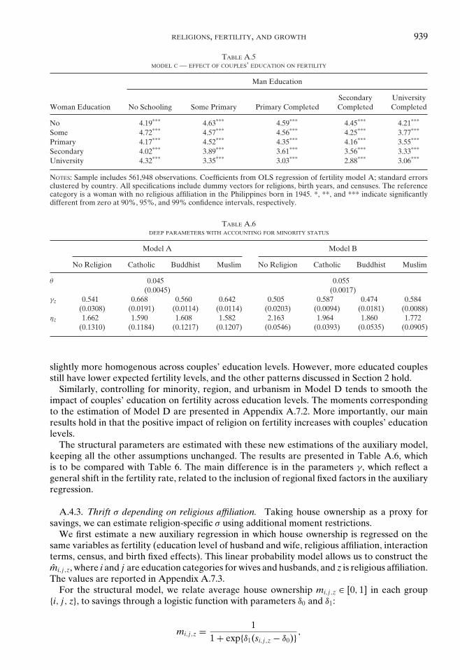
RELIGIONS, FERTILITY, AND GROWTH 939
TABLE A.5MODEL C — EFFECT OF COUPLES’ EDUCATION ON FERTILITY
Man Education
Woman Education No Schooling Some Primary Primary CompletedSecondaryCompleted
UniversityCompleted
No 4.19*** 4.63*** 4.59*** 4.45*** 4.21***
Some 4.72*** 4.57*** 4.56*** 4.25*** 3.77***
Primary 4.17*** 4.52*** 4.35*** 4.16*** 3.55***
Secondary 4.02*** 3.89*** 3.61*** 3.56*** 3.33***
University 4.32*** 3.35*** 3.03*** 2.88*** 3.06***
NOTES: Sample includes 561,948 observations. Coefficients from OLS regression of fertility model A; standard errorsclustered by country. All specifications include dummy vectors for religions, birth years, and censuses. The referencecategory is a woman with no religious affiliation in the Philippines born in 1945. *, **, and *** indicate significantlydifferent from zero at 90%, 95%, and 99% confidence intervals, respectively.
TABLE A.6DEEP PARAMETERS WITH ACCOUNTING FOR MINORITY STATUS
Model A Model B
No Religion Catholic Buddhist Muslim No Religion Catholic Buddhist Muslim
θ 0.045 0.055(0.0045) (0.0017)
γz 0.541 0.668 0.560 0.642 0.505 0.587 0.474 0.584(0.0308) (0.0191) (0.0114) (0.0114) (0.0203) (0.0094) (0.0181) (0.0088)
ηz 1.662 1.590 1.608 1.582 2.163 1.964 1.860 1.772(0.1310) (0.1184) (0.1217) (0.1207) (0.0546) (0.0393) (0.0535) (0.0905)
slightly more homogenous across couples’ education levels. However, more educated couplesstill have lower expected fertility levels, and the other patterns discussed in Section 2 hold.
Similarly, controlling for minority, region, and urbanism in Model D tends to smooth theimpact of couples’ education on fertility across education levels. The moments correspondingto the estimation of Model D are presented in Appendix A.7.2. More importantly, our mainresults hold in that the positive impact of religion on fertility increases with couples’ educationlevels.
The structural parameters are estimated with these new estimations of the auxiliary model,keeping all the other assumptions unchanged. The results are presented in Table A.6, whichis to be compared with Table 6. The main difference is in the parameters γ, which reflect ageneral shift in the fertility rate, related to the inclusion of regional fixed factors in the auxiliaryregression.
A.4.3. Thrift σ depending on religious affiliation. Taking house ownership as a proxy forsavings, we can estimate religion-specific σ using additional moment restrictions.
We first estimate a new auxiliary regression in which house ownership is regressed on thesame variables as fertility (education level of husband and wife, religious affiliation, interactionterms, census, and birth fixed effects). This linear probability model allows us to construct themi,j,z, where i and j are education categories for wives and husbands, and z is religious affiliation.The values are reported in Appendix A.7.3.
For the structural model, we relate average house ownership mi,j,z ∈ [0, 1] in each group{i, j, z}, to savings through a logistic function with parameters δ0 and δ1:
mi,j,z = 11 + exp{δ1(si,j,z − δ0)} ,

940 DE LA CROIX AND DELAVALLADE
TABLE A.7ESTIMATION OF THE DEEP PARAMETERS WITH (15)
No Religion Catholic Buddhist Muslim
θ 0.054(0.0010)
δ0 1.184(0.1326)
δ1 0.628(0.1708)
γz 0.732 0.717 0.601 0.638(0.1136) (0.0330) (0.0437) (0.0558)
ηz 2.119 1.930 1.851 1.737(0.0418) (0.0262) (0.0316) (0.0397)
σz 0.411 0.251 0.274 0.176(0.2001) (0.0556) (0.0847) (0.01035)
NOTE: Mean (SD) of structural parameters minimizing Function (9) for 200 draws of the fertility matrices Ni,j,z.
while savings are given by Equation A.3 from Appendix A.1:
st = σz
1 + σz + γz(ωhf
i + hmj ).
These two equations give a theoretical house ownership rate m�[θ, γz, ηz, σz, hf (i), hm(j)] thatdepends on religion-specific thrift σz. The minimization problem of the structural estimationcan be written as
minθ,γz,ηz,σz,δ0,δ1
∑z
∑i,j
[pi,j,z
(Ni,j,z − n�
[θ, γz, ηz, σz, hf (i), hm(j)
])2
+pi,j,z
(mi,j,z − m�
[θ, γz, ηz, σz, hf (i), hm(j)
])2]
.
Compared to Equation (9), we have additional parameters to estimate, the σzs, and additionalmoments to match, based on house ownership mi,j,z. The results are presented in Table A.7.
A.5. Regression Results. See the Online Appendix on the authors’ website.21
A.6. Robustness to Removing the Philippines and Thailand from the Sample. See the OnlineAppendix on the authors’ website.
21 http://www.de-la-croix.be/appendix/ier18-appendix.pdf
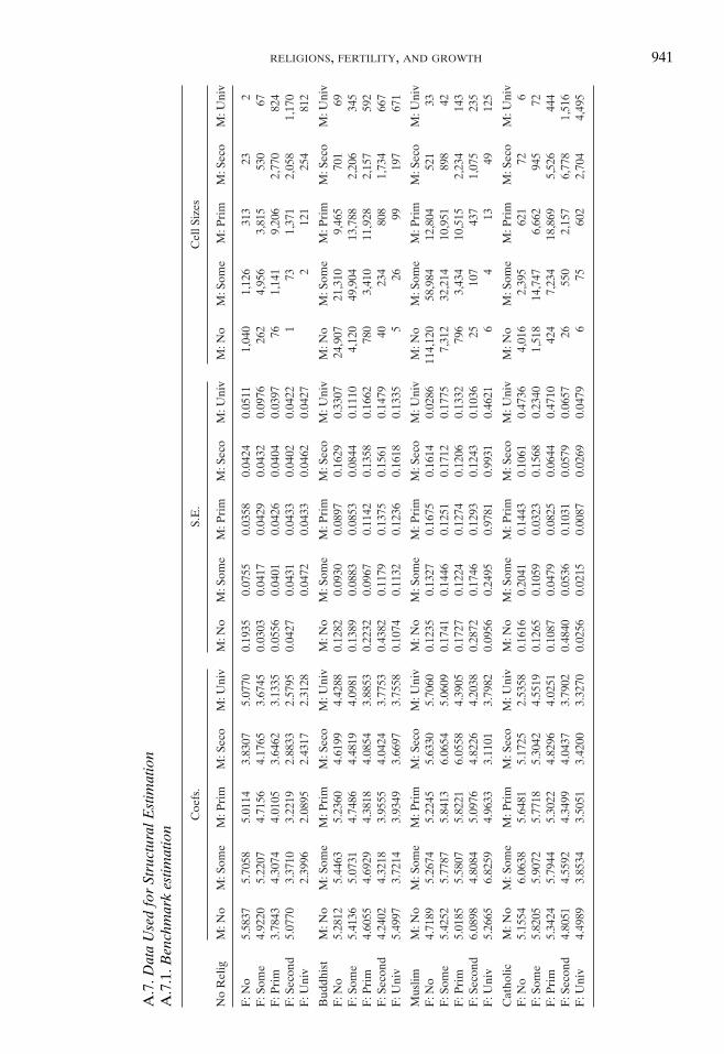
RELIGIONS, FERTILITY, AND GROWTH 941
A.7
.DataUsedforStructuralEstimation
A.7
.1.B
enchmarkestim
ation
Coe
fs.
S.E
.C
ellS
izes
No
Rel
igM
:No
M:S
ome
M:P
rim
M:S
eco
M:U
niv
M:N
oM
:Som
eM
:Pri
mM
:Sec
oM
:Uni
vM
:No
M:S
ome
M:P
rim
M:S
eco
M:U
niv
F:N
o5.
5837
5.70
585.
0114
3.83
075.
0770
0.19
350.
0755
0.03
580.
0424
0.05
111,
040
1,12
631
323
2F
:Som
e4.
9220
5.22
074.
7156
4.17
653.
6745
0.03
030.
0417
0.04
290.
0432
0.09
7626
24,
956
3,81
553
067
F:P
rim
3.78
434.
3074
4.01
053.
6462
3.13
350.
0556
0.04
010.
0426
0.04
040.
0397
761,
141
9,20
62,
770
824
F:S
econ
d5.
0770
3.37
103.
2219
2.88
332.
5795
0.04
270.
0431
0.04
330.
0402
0.04
221
731,
371
2,05
81,
170
F:U
niv
2.39
962.
0895
2.43
172.
3128
0.04
720.
0433
0.04
620.
0427
212
125
481
2
Bud
dhis
tM
:No
M:S
ome
M:P
rim
M:S
eco
M:U
niv
M:N
oM
:Som
eM
:Pri
mM
:Sec
oM
:Uni
vM
:No
M:S
ome
M:P
rim
M:S
eco
M:U
niv
F:N
o5.
2812
5.44
635.
2360
4.61
994.
4288
0.12
820.
0930
0.08
970.
1629
0.33
0724
,907
21,3
109,
465
701
69F
:Som
e5.
4136
5.07
314.
7486
4.48
194.
0981
0.13
890.
0883
0.08
530.
0844
0.11
104,
120
49,9
0413
,788
2,20
634
5F
:Pri
m4.
6055
4.69
294.
3818
4.08
543.
8853
0.22
320.
0967
0.11
420.
1358
0.16
6278
03,
410
11,9
282,
157
592
F:S
econ
d4.
2402
4.32
183.
9555
4.04
243.
7753
0.43
820.
1179
0.13
750.
1561
0.14
7940
234
808
1,73
466
7F
:Uni
v5.
4997
3.72
143.
9349
3.66
973.
7558
0.10
740.
1132
0.12
360.
1618
0.13
355
2699
197
671
Mus
limM
:No
M:S
ome
M:P
rim
M:S
eco
M:U
niv
M:N
oM
:Som
eM
:Pri
mM
:Sec
oM
:Uni
vM
:No
M:S
ome
M:P
rim
M:S
eco
M:U
niv
F:N
o4.
7189
5.26
745.
2245
5.63
305.
7060
0.12
350.
1327
0.16
750.
1614
0.02
8611
4,12
058
,984
12,8
0452
133
F:S
ome
5.42
525.
7787
5.84
136.
0654
5.06
090.
1741
0.14
460.
1251
0.17
120.
1775
7,31
232
,214
10,9
5189
842
F:P
rim
5.01
855.
5807
5.82
216.
0558
4.39
050.
1727
0.12
240.
1274
0.12
060.
1332
796
3,43
410
,515
2,23
414
3F
:Sec
ond
6.08
984.
8084
5.09
764.
8226
4.20
380.
2872
0.17
460.
1293
0.12
430.
1036
2510
743
71,
075
235
F:U
niv
5.26
656.
8259
4.96
333.
1101
3.79
820.
0956
0.24
950.
9781
0.99
310.
4621
64
1349
125
Cat
holic
M:N
oM
:Som
eM
:Pri
mM
:Sec
oM
:Uni
vM
:No
M:S
ome
M:P
rim
M:S
eco
M:U
niv
M:N
oM
:Som
eM
:Pri
mM
:Sec
oM
:Uni
vF
:No
5.15
546.
0638
5.64
815.
1725
2.53
580.
1616
0.20
410.
1443
0.10
610.
4736
4,01
62,
395
621
726
F:S
ome
5.82
055.
9072
5.77
185.
3042
4.55
190.
1265
0.10
590.
0323
0.15
680.
2340
1,51
814
,747
6,66
294
572
F:P
rim
5.34
245.
7944
5.30
224.
8296
4.02
510.
1087
0.04
790.
0825
0.06
440.
4710
424
7,23
418
,869
5,52
644
4F
:Sec
ond
4.80
514.
5592
4.34
994.
0437
3.79
020.
4840
0.05
360.
1031
0.05
790.
0657
2655
02,
157
6,77
81,
516
F:U
niv
4.49
893.
8534
3.50
513.
4200
3.32
700.
0256
0.02
150.
0087
0.02
690.
0479
675
602
2,70
44,
495
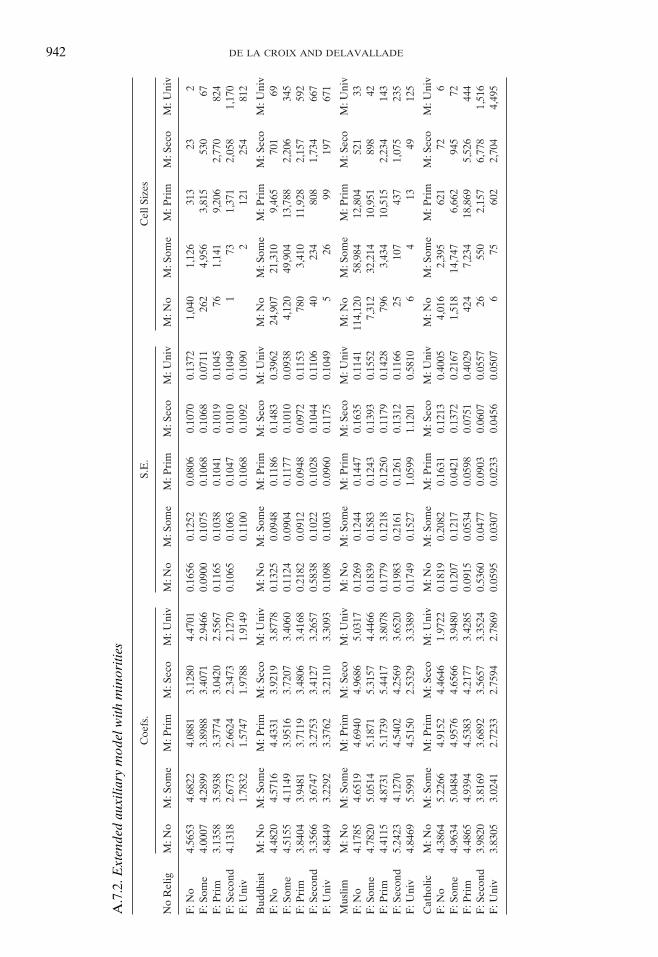
942 DE LA CROIX AND DELAVALLADE
A.7
.2.E
xtendedauxiliarymodelwith
minorities
Coe
fs.
S.E
.C
ellS
izes
No
Rel
igM
:No
M:S
ome
M:P
rim
M:S
eco
M:U
niv
M:N
oM
:Som
eM
:Pri
mM
:Sec
oM
:Uni
vM
:No
M:S
ome
M:P
rim
M:S
eco
M:U
niv
F:N
o4.
5653
4.68
224.
0881
3.12
804.
4701
0.16
560.
1252
0.08
060.
1070
0.13
721,
040
1,12
631
323
2F
:Som
e4.
0007
4.28
993.
8988
3.40
712.
9466
0.09
000.
1075
0.10
680.
1068
0.07
1126
24,
956
3,81
553
067
F:P
rim
3.13
583.
5938
3.37
743.
0420
2.55
670.
1165
0.10
380.
1041
0.10
190.
1045
761,
141
9,20
62,
770
824
F:S
econ
d4.
1318
2.67
732.
6624
2.34
732.
1270
0.10
650.
1063
0.10
470.
1010
0.10
491
731,
371
2,05
81,
170
F:U
niv
1.78
321.
5747
1.97
881.
9149
0.11
000.
1068
0.10
920.
1090
212
125
481
2
Bud
dhis
tM
:No
M:S
ome
M:P
rim
M:S
eco
M:U
niv
M:N
oM
:Som
eM
:Pri
mM
:Sec
oM
:Uni
vM
:No
M:S
ome
M:P
rim
M:S
eco
M:U
niv
F:N
o4.
4820
4.57
164.
4331
3.92
193.
8778
0.13
250.
0948
0.11
860.
1483
0.39
6224
,907
21,3
109,
465
701
69F
:Som
e4.
5155
4.11
493.
9516
3.72
073.
4060
0.11
240.
0904
0.11
770.
1010
0.09
384,
120
49,9
0413
,788
2,20
634
5F
:Pri
m3.
8404
3.94
813.
7119
3.48
063.
4168
0.21
820.
0912
0.09
480.
0972
0.11
5378
03,
410
11,9
282,
157
592
F:S
econ
d3.
3566
3.67
473.
2753
3.41
273.
2657
0.58
380.
1022
0.10
280.
1044
0.11
0640
234
808
1,73
466
7F
:Uni
v4.
8449
3.22
923.
3762
3.21
103.
3093
0.10
980.
1003
0.09
600.
1175
0.10
495
2699
197
671
Mus
limM
:No
M:S
ome
M:P
rim
M:S
eco
M:U
niv
M:N
oM
:Som
eM
:Pri
mM
:Sec
oM
:Uni
vM
:No
M:S
ome
M:P
rim
M:S
eco
M:U
niv
F:N
o4.
1785
4.65
194.
6940
4.96
865.
0317
0.12
690.
1244
0.14
470.
1635
0.11
4111
4,12
058
,984
12,8
0452
133
F:S
ome
4.78
205.
0514
5.18
715.
3157
4.44
660.
1839
0.15
830.
1243
0.13
930.
1552
7,31
232
,214
10,9
5189
842
F:P
rim
4.41
154.
8731
5.17
395.
4417
3.80
780.
1779
0.12
180.
1250
0.11
790.
1428
796
3,43
410
,515
2,23
414
3F
:Sec
ond
5.24
234.
1270
4.54
024.
2569
3.65
200.
1983
0.21
610.
1261
0.13
120.
1166
2510
743
71,
075
235
F:U
niv
4.84
695.
5991
4.51
502.
5329
3.33
890.
1749
0.15
271.
0599
1.12
010.
5810
64
1349
125
Cat
holic
M:N
oM
:Som
eM
:Pri
mM
:Sec
oM
:Uni
vM
:No
M:S
ome
M:P
rim
M:S
eco
M:U
niv
M:N
oM
:Som
eM
:Pri
mM
:Sec
oM
:Uni
vF
:No
4.38
645.
2266
4.91
524.
4646
1.97
220.
1819
0.20
820.
1631
0.12
130.
4005
4,01
62,
395
621
726
F:S
ome
4.96
345.
0484
4.95
764.
6566
3.94
800.
1207
0.12
170.
0421
0.13
720.
2167
1,51
814
,747
6,66
294
572
F:P
rim
4.48
654.
9394
4.53
834.
2177
3.42
850.
0915
0.05
340.
0598
0.07
510.
4029
424
7,23
418
,869
5,52
644
4F
:Sec
ond
3.98
203.
8169
3.68
923.
5657
3.35
240.
5360
0.04
770.
0903
0.06
070.
0557
2655
02,
157
6,77
81,
516
F:U
niv
3.83
053.
0241
2.72
332.
7594
2.78
690.
0595
0.03
070.
0233
0.04
560.
0507
675
602
2,70
44,
495

RELIGIONS, FERTILITY, AND GROWTH 943
A.7
.3.H
ouseow
nership
Coe
fs.
S.E
.C
ellS
izes
No
Rel
igM
:No
M:S
ome
M:P
rim
M:S
eco
M:U
niv
M:N
oM
:Som
eM
:Pri
mM
:Sec
oM
:Uni
vM
:No
M:S
ome
M:P
rim
M:S
eco
M:U
niv
F:N
o0.
2965
0.30
650.
3106
0.27
980.
3260
0.05
120.
0359
0.03
200.
0284
0.01
7795
81,
039
292
212
F:S
ome
0.30
580.
2852
0.33
960.
3084
0.31
320.
0352
0.03
510.
0335
0.03
000.
0204
248
4,77
83,
641
508
61F
:Pri
m0.
3944
0.39
200.
4315
0.44
800.
4715
0.03
380.
0342
0.03
250.
0286
0.02
2364
1,00
58,
234
2,49
072
8F
:Sec
ond
1.26
070.
3829
0.47
720.
4663
0.47
240.
0377
0.02
660.
0286
0.02
400.
0206
167
1,23
01,
840
1,03
0F
:Uni
v0.
2565
0.38
010.
5165
0.52
070.
0387
0.02
180.
0227
0.01
882
102
233
703
Bud
dhis
tM
:No
M:S
ome
M:P
rim
M:S
eco
M:U
niv
M:N
oM
:Som
eM
:Pri
mM
:Sec
oM
:Uni
vM
:No
M:S
ome
M:P
rim
M:S
eco
M:U
niv
F:N
o0.
3140
0.31
740.
3242
0.34
450.
3731
0.03
840.
0379
0.03
910.
0429
0.03
6924
,777
21,2
039,
441
701
69F
:Som
e0.
3268
0.32
220.
3205
0.33
190.
3028
0.03
890.
0402
0.03
770.
0332
0.02
934,
087
49,6
9313
,733
2,19
734
3F
:Pri
m0.
3203
0.31
750.
3336
0.34
990.
3516
0.04
560.
0365
0.03
440.
0304
0.02
6877
83,
400
11,8
592,
145
588
F:S
econ
d0.
3409
0.34
550.
3616
0.34
630.
3449
0.04
450.
0355
0.03
120.
0286
0.02
7140
233
803
1,72
865
9F
:Uni
v0.
1559
0.31
880.
3104
0.33
180.
3338
0.03
260.
0282
0.02
780.
0295
0.02
635
2698
196
664
Mus
limM
:No
M:S
ome
M:P
rim
M:S
eco
M:U
niv
M:N
oM
:Som
eM
:Pri
mM
:Sec
oM
:Uni
vM
:No
M:S
ome
M:P
rim
M:S
eco
M:U
niv
F:N
o0.
3616
0.35
790.
3361
0.30
270.
3740
0.03
690.
0362
0.03
580.
0389
0.02
8411
3,89
158
,942
12,7
7250
829
F:S
ome
0.35
820.
3463
0.32
190.
2982
0.32
530.
0343
0.03
460.
0341
0.03
560.
0542
7,29
932
,138
10,9
0289
039
F:P
rim
0.36
090.
3275
0.28
280.
2248
0.19
560.
0409
0.03
390.
0362
0.03
550.
0533
790
3,41
910
,464
2,22
213
9F
:Sec
ond
0.26
880.
2937
0.20
990.
1230
0.03
250.
0146
0.03
460.
0363
0.03
340.
0449
2410
543
01,
050
232
F:U
niv
0.41
470.
3682
0.33
740.
2403
0.18
430.
1141
0.10
810.
0390
0.00
870.
1076
44
1144
107
Cat
holic
M:N
oM
:Som
eM
:Pri
mM
:Sec
oM
:Uni
vM
:No
M:S
ome
M:P
rim
M:S
eco
M:U
niv
M:N
oM
:Som
eM
:Pri
mM
:Sec
oM
:Uni
vF
:No
0.34
030.
3548
0.32
690.
3406
ezw
r0.
0280
0.02
570.
0332
0.13
770.
2748
3,88
22,
270
580
666
F:S
ome
0.36
180.
3652
0.36
190.
3314
0.44
120.
0301
0.02
660.
0304
0.03
740.
0331
1,38
413
,410
6,04
886
566
F:P
rim
0.36
000.
3662
0.33
190.
2927
0.28
030.
0285
0.02
730.
0246
0.01
960.
0390
387
6,51
217
,271
5,12
140
1F
:Sec
ond
0.21
850.
3419
0.31
770.
2414
0.25
310.
0252
0.02
420.
0149
0.01
370.
0197
2349
31,
973
6,38
71,
432
F:U
niv
0.74
630.
3518
0.36
230.
3366
0.30
190.
0099
0.02
080.
0175
0.01
070.
0109
463
553
2,46
84,
131
675
602
2,70
44,
495

944 DE LA CROIX AND DELAVALLADE
REFERENCES
ACEMOGLU, D., AND J. ANGRIST, “How Large Are Human Capital Externalities? Evidence from Compul-sory Schooling Laws,” in B. Bernanke and K. Rogoff, eds., NBER Macroeconomics Annual (Cam-bridge, MA: MIT Press, 2001), 9–59.
ADSERA, A., “Marital Fertility and Religion in Spain, 1985 and 1999,” Population Studies 60(2) (2006a),205–21.
———, “Religion and Changes in Family-Size Norms in Developed Countries,” Review of ReligiousResearch 47(3) (2006b), 271–86.
ALESINA, A., P. GIULIANO, AND N. NUNN, “On the Origins of Gender Roles: Women and the Plough,” TheQuarterly Journal of Economics 128 (2013), 469–530.
BAR, M., M. HAZAN, O. LEUKHINA, D. WEISS, AND H ZOABI, “Is the Market Pronatalist? Inequality,Differential Fertility, and Growth Revisited,” CEPR Discussion Papers 12376 (2017).
BARRO, R. J., AND R. MCCLEARY, “Religion and Economic Growth,” Technical Report 9682, NationalBureau of Economic Research, 2003.
BAUDIN, T., “A Role for Cultural Transmission in Fertility Transitions,” Macroeconomic Dynamics 14(4)(2010), 454–81.
———, “Religion and Fertility: The French Connection,” Demographic Research 32 (2015), 397–420.BECKER, G., “Nobel Lecture: The Economic Way of Looking at Behavior,” Journal of Political Economy
101(3) (1993), 385–409.BECKER, S. O., AND L. WOESSMANN, “Was Weber Wrong? A Human Capital Theory of Protestant Economic
History,” The Quarterly Journal of Economics 124(2) (2009), 531–96.BERMAN, E., L. R. IANNACCONE, AND G. RAGUSA, “From Empty Pews to Empty Cradles: Fertility Decline
among European Catholics,” Journal of Demographic Economics 84 (2018, forthcoming).BHATTACHARYA, J., AND S. CHAKRABORTY, “Contraception and the Fertility Transition,” Economics Work-
ing Papers 2002–2016, Iowa State University, 2013.BISIN, A., AND T. VERDIER, “The Economics of Cultural Transmission and Socialization,” technical report,
National Bureau of Economic Research, 2010.Blyth, E., and R. Landau, eds., Faith and Fertility: Attitudes Towards Reproductive Practices in Different
Religions from Ancient to Modern Times (London: Jessica Kingsley Publishers, 2009).BOLT, J., AND J. L. VAN ZANDEN, “The First Update of the Maddison Project; Re-estimating Growth Before
1820,” Maddison Project Working Paper 4, 2013.BOPPART, T., J. FALKINGER, V. GROSSMANN, U. WOITEK, AND G. WUTHRICH, “Under Which Conditions
Does Religion Affect Educational Outcomes?” Explorations in Economic History 50(2) (2013),242–66.
BROWNING, M., P.-A. CHIAPPORI, AND Y. WEISS, Economics of the Family (Cambridge MA: CambridgeUniversity Press, 2014).
CAVALCANTI, T., S. PARENTE, AND R. ZHAO, “Religion in Macroeconomics: A Quantitative Analysis ofWeber’s Thesis,” Economic Theory 32(1) (2007), 105–23.
CERVELLATI, M., M. JANSEN, AND U. SUNDE, “Religious Norms and Long Term Development: Insurance,Human Capital and Technological Change,” Paper presented at Barcelona GSE Summer Forum,2014.
CHABE-FERRET, B., “Adherence to Cultural Norms and Economic Incentives: Evidence from Fertility Tim-ing Decisions,” Technical Report 2016-23, Universite catholique de Louvain, Institut de RecherchesEconomiques et Sociales (IRES), 2016.
———, AND P. MELINDI GHIDI, “Differences in Fertility Behavior and Uncertainty: An Economic Theoryof the Minority Status Hypothesis,” Journal of Population Economics 26(3) (2013), 887–905.
COHEN, D., AND M. SOTO, “Growth and Human Capital: Good Data, Good Results,” Journal of EconomicGrowth 12(1) (2007), 51–76.
CORDOBA, J., AND M. RIPOLL, “Intergenerational Transfers and the Fertility-Income Relationship,” Eco-nomic Journal 126 (2016), 949–77.
DE LA CROIX, D., AND M. DOEPKE, “Inequality and Growth: Why Differential Fertility Matters,” AmericanEconomic Review 93(4) (2003), 1091–113.
DOEPKE, M., “Child Mortality and Fertility Decline: Does the Barro–Becker Model Fit the Facts?” Journalof Population Economics 18(2) (2005), 337–66.
———, “Gary Becker on the Quantity and Quality of Children,” Journal of Demographic Economics 81(2015), 59–66.
———, M. HAZAN, AND Y. MAOZ, “The Baby Boom and World War II: A Macroeconomic Analysis,”Review of Economic Studies 82 (2015), 1031–73.
DURLAUF, S. N., A. KOURTELLOS, AND C. M. TAN, “Is God in the Details? A Reexamination of the Role ofReligion in Economic Growth,” Technical Report 0613, Department of Economics, Tufts University,2006.

RELIGIONS, FERTILITY, AND GROWTH 945
GALOR, O., AND O. MOAV, “Das Human-Kapital: A Theory of the Demise of the Class Structure,” Reviewof Economic Studies 73(1) (2006), 85–117.
GOBBI, P., “Childcare and Commitment within Households,” Journal of Economic Theory 176 (2018),503–551.
GOURIEROUX, C., A. MONFORT, AND E. RENAULT, “Indirect Inference,” Journal of Applied Econometrics8(S) (1993), S85–118.
GUISO, L., P. SAPIENZA, AND L. ZINGALES, “People’s Opium? Religion and Economic Attitudes,” Journalof Monetary Economics 50(1) (2003), 225–82.
HANUSHEK, E. A., AND L. WOESSMANN, “Do Better Schools Lead to More Growth? Cognitive Skills,Economic Outcomes, and Causation,” Journal of Economic Growth 17(4) (2012), 267–321.
HAZAN, M., AND H. ZOABI, “Sons or Daughters? Sex Preferences and the Reversal of the Gender Educa-tional Gap,” Journal of Demographic Economics 81 (2015), 179–201.
HEATON, T. B., “Does Religion Influence Fertility in Developing Countries” Population Research andPolicy Review 30(3) (2011), 449–65.
HOTZ, V. J., S. W. MCELROY, AND S. G. SANDERS, “Teenage Childbearing and Its Life Cycle Consequences:Exploiting a Natural Experiment,” Journal of Human Resources 40(3) (2005), 683–715.
JEJEEBHOY, S. J.,Women’sEducation,Autonomy,andReproductiveBehaviour:Experience fromDevelopingCountries (New York: Oxford University Press, 1995).
KLEMP, M., AND J. WEISDORF, “Fecundity, Fertility, and the Formation of Human Capital,” The EconomicJournal (2018, forthcoming). https://doi.org/10.1111/ecoj.12589.
KRUEGER, A., AND M. LINDAHL, “Education and Growth: Why and for Whom?” Journal of EconomicLiterature 39(4) (2001), 1101–36.
LAGERLOF, N.-P., “The Galor-Weil Model Revisited: A Quantitative Exercise,” Review of EconomicDynamics 9(1) (2006), 116–42.
LEE, G. L., C. H. Y. CHAN, E. W.-H. C. HUI, AND C. L. W. CHAN, “Chinese Traditional Belief Systems,Livelihood and Fertility,” in E. Blyth and R. Landau, eds., Faith and Fertility: Attitudes TowardsReproductive Practices inDifferent Religions fromAncient toModernTimes (London: Jessica KingsleyPublishers, 2009), 137–57.
LEHRER, E. L., “Religion as a Determinant of Economic and Demographic Behavior in the United States,”Population and Development Review 30(4) (2004), 707–26.
LEIBOWITZ, A., “Home Investments in Children,” Journal of Political Economy 82(2) (1974), S111–31.LI, H., J. ZHANG, AND Y. ZHU, “The Quantity–Quality Trade-Off of Children in a Developing Country:
Identification Using Chinese Twins,” Demography 45(1) (2008), 223–43.LIN, W., AND J. PANTANO, “The Unintended: Negative Outcomes over the Life Cycle,” Journal of Population
Economics 28(2) (2015), 479–508.LONG, J. S., AND J. FREESE,RegressionModels for Categorical Dependent Variables Using Stata, 2nd edition
(College Station: Stata Press, 2006).LUCAS, R., “Making a Miracle,” Econometrica 61(2) (1993), 251–72.LUO, X., AND T. TERADA, “Education and Wage Differentials in the Philippines,” Technical Report 5120,
The World Bank, 2009.MADDISON, A., “Historical Statistics,” Groningen Growth and Development Center, 2010.MCCLEARY, R. M., “Protestantism and Human Capital in Guatemala and the Republic of Korea,” Adb
Economics Working Paper 332, Asian Development Bank, 2013.MINNESOTA POPULATION CENTER. “Integrated Public Use Microdata Series, International: Version 6.2.”
[Machine-readable database]. Minneapolis: University of Minnesota, 2013.MOAV, O., “Cheap Children and the Persistence of Poverty,” Economic Journal 115(500) (2005), 88–
110.MONTENEGRO, C. E., AND H. A. PATRINOS, “Comparable Estimates of Returns to Schooling around the
World,” Policy Research Working Paper 7020, The World Bank, 2014.MOSHER, W. D., L. B. WILLIAMS, AND D. P. JOHNSON DAVID, “Religion and Fertility in the United States:
New Patterns,” Demography 29(2) (1992), 199–214.MUNSHI, K., AND J. MYAUX, “Social Norms and the Fertility Transition,” Journal ofDevelopment Economics
80(1) (2006), 1–38.PUTTERMAN, L., “Agricultural Transition Year Country Data Set,” Brown University, 2006.RANGAZAS, P., “Schooling and Economic Growth: A King–Rebelo Experiment with Human Capital,”
Journal of Monetary Economics 46(2) (2000), 397–416.RIBAR, D. C., “Teenage Fertility and High School Completion,” The Review of Economics and Statistics
76(3) (1994), 413–24.SANDER, W., “Catholicism and the Economics of Fertility,” Population Studies: A Journal of Demography
46 (1992), 477–89.SKIRBEKK, V., M. STONAWSKI, S. FUKUDA, T. SPOORENBERG, C. HACKETT, AND R. MUTTARAK, “Is Buddhism
the Low Fertility Religion of Asia?” Demographic Research 32 (2015), 1–28.

946 DE LA CROIX AND DELAVALLADE
SMITH, A. A., JR., “Indirect Inference,” in S. N. Durlauf and L. E. Blume, eds.,TheNewPalgraveDictionaryof Economics (London: Palgrave Macmillan, 2008).
STRULIK, H., “From Worship to Worldly Pleasures: Secularization and Long-Run Economic Growth,”Technical Report 116, Courant Research Centre PEG, 2012.
TAMURA, R., “Teachers, Growth and Convergence,” Journal of Political Economy 109(5) (2001), 1021–59.———, “Human Capital and Economic Development,” Journal of Development Economics 79 (2006),
26–72.———, S. CURTIS, AND K. M. MURPHY, “Black and White Fertility, Differential Baby Booms: The Value
of Equal Education Opportunity,” Journal of Demographic Economics 82(1) (2016), 27–109.VOGL, T., “Differential Fertility, Human Capital, and Development,” Review of Economic Studies 83
(2016), 365–401.ZHANG, L., “Religious Affiliation, Religiosity, and Male and Female Fertility,” Demographic Research 18
(2008), 233–62.