Embed Size (px)
Citation preview
RELIABLE SOLUTION OF CONVEX QUADRATIC PROGRAMSWITH PARAMETRIC ACTIVE SET METHODS
A. POTSCHKA∗, C. KIRCHES∗ , H. G. BOCK∗ , AND J. P. SCHLODER∗
Abstract. Parametric Active Set Methods (PASM) are a relatively new class of methods tosolve convex Quadratic Programming (QP) problems. They are based on tracing the solution along alinear homotopy between a QP with known solution and the QP to be solved. We explicitly identifynumerical challenges in PASM and develop strategies to meet these challenges. To demonstrate thereliability improvements of the proposed strategies we have implemented a prototype code calledrpasm. We compare the results of the code with those of other popular academic and commercialQP solvers on problems of a subset of the Maros-Meszaros test examples. Our code is the only oneto solve all of the problems with the default settings. Furthermore, we propose how PASM can beused to compute local solutions of nonconvex QPs.
Key words. active set, convex, homotopy method, parametric quadratic programming
AMS subject classifications. 90C20, 90C25, 97N60, 97N80
1. Introduction. This paper is dedicated to the numerical solution of the con-vex quadratic programming (QP) problem
minx∈Rn
1
2xTBx+ bTx s. t. cl ≤ Cx ≤ cu, (1.1)
with symmetric positive semidefinite Hessian matrix B ∈ Rn×n, constraint matrixC ∈ Rm×n, gradient vector b ∈ Rn, and lower and upper constraint vectors cl, cu ∈Rm. Throughout this paper, inequality signs between vectors are to be understoodelementwise.
The class of convex QP problems is important in its own right. Gould and Tointhave been compiling a bibliography [19] of currently 979 publications which comprisesmany application papers from disciplines as diverse as portfolio analysis, structuralanalysis, VLSI design, discrete-time stabilization, optimal and fuzzy control, finiteimpluse response design, optimal power flow, economic dispatch, etc. Several bench-mark and application problems are collected in a repository [25] which is accessiblethrough the CUTEr testing environment [17]. Furthermore, QPs arise as subprob-lems in Sequential Quadratic Programming (SQP), a state-of-the-art method for thesolution of nonlinear optimization problems.
1.1. Optimality conditions. For the characterization of solutions of QP (1.1)we partition the index set m = {1, . . . ,m} into four disjoint sets
Ae(x) = {i ∈ m | cli = (Cx)i = cui }, Al(x) = {i ∈ m | cli = (Cx)i < cui },Au(x) = {i ∈ m | cli < (Cx)i = cui }, Af(x) = {i ∈ m | cli < (Cx)i < cui }
of equality, lower active, upper active, and free constraint indices, respectively. It iswell known (see, e.g., [29]) that for any solution x∗ of QP (1.1) there exists a vector
∗Interdisciplinary Center for Scientific Computing, Heidelberg University, Im Neuenheimer Feld368, 69120 Heidelberg, Germany ([email protected]).
1
2 A. POTSCHKA, C. KIRCHES, H. G. BOCK, AND J. P. SCHLODER
y∗ ∈ Rm of so called Lagrange multipliers or dual variables such that
Bx∗ + b− CTy∗ = 0, cl ≤ Cx∗ ≤ cu, (1.2a)
(Cx∗ − cl)iy∗i = 0, i ∈ Al(x∗), y∗i ≥ 0, i ∈ Al(x∗), (1.2b)
(Cx∗ − cu)iy∗i = 0, i ∈ Au(x∗), y∗i ≤ 0, i ∈ Au(x∗). (1.2c)
Conversely, every primal-dual pair (x∗, y∗) which satisfies conditions (1.2) is a globalsolution of QP (1.1) due to semidefiniteness of the Hessian matrix B. The solution isunique if and only if the following two conditions are satisfied:
1. The active constraint rows Ci, i ∈ Ae ∪ Al ∪ Au, are linearly independent.2. Matrix B is positive definite on the null space of the active constraints.
1.2. Existing methods. All existing methods for solving QPs are iterative andcan be grossly divided into Active Set and Interior Point methods. Interior Pointmethods are sometimes called Barrier methods due to the possibility of differentinterpretations of the resulting subproblems (see, e.g., [29]). As a defining feature,Active Set methods keep a working set of active constraints and solve a sequence ofequality constrained QPs. The working set must be updated between the iteratesaccording to exchange rules which are based on conditions (1.2). In contrast, InteriorPoint methods do not use a working set but follow a nonlinear path, the so calledcentral path, from a strictly feasible point towards the solution.
Active Set methods can be divided into primal, dual, and parametric methods, ofwhich the primal Active Set method is the oldest and can be seen as a direct extensionof the Simplex Algorithm [6]. Dual Active Set methods apply the primal Active Setmethod to the dual of QP (1.1) (which exists due to convexity). A relatively newvariant of an Active Set method are Parametric Active Set Methods (PASM), e.g.,the Parametric Quadratic Programming (PQP) method [3], which are the methodsof interest in this paper. It is based on an affine-linear homotopy between a QP withknown solution and the QP to be solved. It turns out that the optimal solutionsdepend piecewise affine-linear on the homotopy parameter and that along each affine-linear segment the active set is constant. The iterates of the method are simply thestart points of each segment.
The numerical behaviour of Active Set and Interior Point methods is usually quitedifferent: While Active Set methods need on average substantially more iterationsthan Interior Point methods, the numerical effort for one iteration is substantiallyless for Active Set methods. Often, one or the other method will perform favorablyon a certain problem instance, underlining that both approaches are important.
We want to concisely compare the main advantages of the different Active Setversus Interior Point methods. One advantage of Interior Point methods is the reg-ularizing effect of the central path which leads to well-defined behavior on problemswith nonunique solutions due to, e.g., degeneracy or zero curvature in a feasible direc-tion at the solution. An advantage of all Active Set methods is the possibility of hotstarts which can give a substantial speed-up when solving a sequence of related QPsbecause the active set between the solutions usually changes only slightly. A uniqueadvantage of PASM is that the so called Phase 1 is not needed. The term Phase1 describes the solution of an auxiliary problem to find a feasible starting point forprimal and dual Active Set methods or a strictly feasible starting point for InteriorPoint methods. The generation of an appropriate starting point with Phase 1 can beas expensive as the subsequent solution of the actual problem.
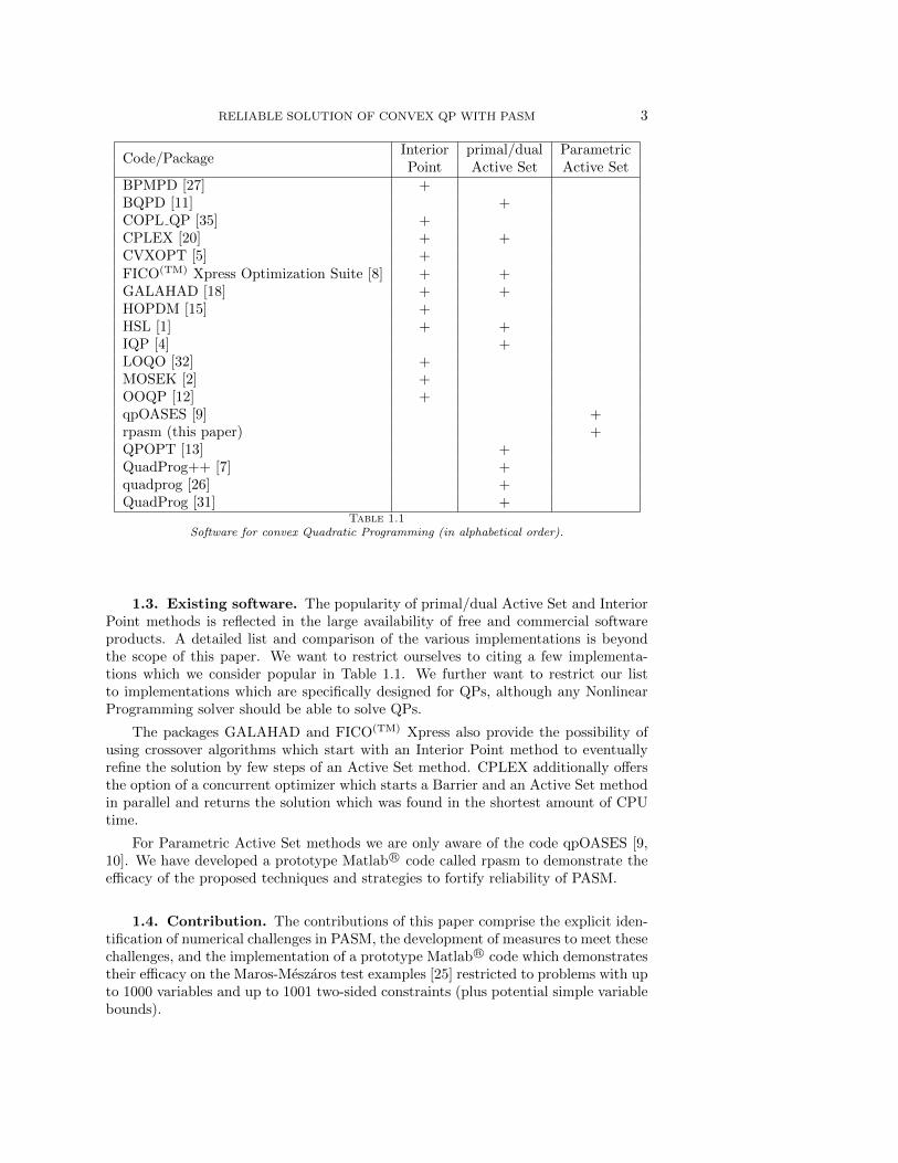
RELIABLE SOLUTION OF CONVEX QP WITH PASM 3
Code/PackageInterior primal/dual ParametricPoint Active Set Active Set
BPMPD [27] +BQPD [11] +COPL QP [35] +CPLEX [20] + +CVXOPT [5] +FICO(TM) Xpress Optimization Suite [8] + +GALAHAD [18] + +HOPDM [15] +HSL [1] + +IQP [4] +LOQO [32] +MOSEK [2] +OOQP [12] +qpOASES [9] +rpasm (this paper) +QPOPT [13] +QuadProg++ [7] +quadprog [26] +QuadProg [31] +
Table 1.1Software for convex Quadratic Programming (in alphabetical order).
1.3. Existing software. The popularity of primal/dual Active Set and InteriorPoint methods is reflected in the large availability of free and commercial softwareproducts. A detailed list and comparison of the various implementations is beyondthe scope of this paper. We want to restrict ourselves to citing a few implementa-tions which we consider popular in Table 1.1. We further want to restrict our listto implementations which are specifically designed for QPs, although any NonlinearProgramming solver should be able to solve QPs.
The packages GALAHAD and FICO(TM) Xpress also provide the possibility ofusing crossover algorithms which start with an Interior Point method to eventuallyrefine the solution by few steps of an Active Set method. CPLEX additionally offersthe option of a concurrent optimizer which starts a Barrier and an Active Set methodin parallel and returns the solution which was found in the shortest amount of CPUtime.
For Parametric Active Set methods we are only aware of the code qpOASES [9,10]. We have developed a prototype Matlab R© code called rpasm to demonstrate theefficacy of the proposed techniques and strategies to fortify reliability of PASM.
1.4. Contribution. The contributions of this paper comprise the explicit iden-tification of numerical challenges in PASM, the development of measures to meet thesechallenges, and the implementation of a prototype Matlab R© code which demonstratestheir efficacy on the Maros-Meszaros test examples [25] restricted to problems with upto 1000 variables and up to 1001 two-sided constraints (plus potential simple variablebounds).
4 A. POTSCHKA, C. KIRCHES, H. G. BOCK, AND J. P. SCHLODER
1.5. Structure of the article. We start with recalling the Parametric QuadraticProgramming (PQP) method [3] in §2 and identify its fundamental numerical chal-lenges in §3. In §4 we develop strategies to meet these challenges. It follows a shortdescription of the newly developed Matlab R© code rpasm in §5 which we compare withother popular academic and commercial QP solvers in §6. We continue in §7 with adescription of drawbacks of the reliability improving strategies. In §8 we discuss anextension to compute local minima of nonconvex QPs before we close the paper withconclusions and an outlook in §9.
2. Parametric Active Set methods.
2.1. The Parametric QP. The idea behind Parametric Active Set methodsconsists of following the optimal solutions on a homotopy path between two QPinstances. Figuratively speaking, the homotopy morphs a QP with known solutioninto the QP to be solved. Let this homotopy be parametrized by τ ∈ [0, 1]. We thenwant to solve the one-parametric family of QP problems
minx(τ)∈Rn
1
2x(τ)TBx(τ) + b(τ)Tx(τ) s. t. cl(τ) ≤ Cx(τ) ≤ cu(τ), (2.1)
with b, cl, and cu now being continuous functions b(τ), cl(τ), cu(τ). For fixed τ , letthe optimal primal-dual solution be denoted by z(τ) = (x(τ), y(τ)) which necessarilysatisfies (1.2) (with b = b(τ), cl = cl(τ), cu = cu(τ)). If we furthermore restrict thehomotopy to affine-linear functions b ∈ Hn, cl, cu ∈ Hm, where
Hk = {f : [0, 1]→ R | f(τ) = (1− τ)f(0) + τf(1), τ ∈ [0, 1]},
it turns out that the optimal solutions z(τ) depend piecewise linearly but not necessar-ily continuous on τ [3]. On each linear segment the active set is constant. ParametricActive Set algorithms follow z(τ) by jumping from one beginning of a segment to thenext. We can immediately observe that this approach allows hot-starts in a naturalway. As mentioned already in §1.2, no Phase 1 is needed to begin the method: We canalways recede to the homotopy start b(0) = 0, cl(0) = 0, cu(0) = 0, x(0) = 0, y(0) = 0,although this is certainly not the best choice as we will discuss in §3 and §4.
2.2. The Parametric Quadratic Programming algorithm. A Paramet-ric Active Set method was first described by Best [3] under the name ParametricQuadratic Programming (PQP) algorithm. Algorithm 1 displays the main steps. Thelines preceded by a number deserve further explanation.
Step 1: Computation of step direction. The working set W is encoded as an m-vector with entries 0 or ±1, where the i-th component indicates whether constraint i isinactive (Wi = 0), active at the lower bound (Wi = −1), or active at the upper bound(Wi = +1). Let CW denote the matrix consisting of the rows Ci with Wi 6= 0 andlet cW (τ) denote a vector which consists of entries cli(τ) or cui (τ) depending on which(if any) bound is marked active in Wi. We can then determine the step direction(∆x,∆y) by solving
KW (τ)
(∆x−∆yW
):=
(B CT
W
CW 0
)(∆x−∆yW
)=
(−(b(1)− b(τ))cW (1)− cW (τ)
). (2.2)
The dual step ∆y must be assembled from ∆yW by filling in zeros at the entries ofconstraints i which are not in the working set (i.e., Wi = 0). For the initial workingset W we assume matrix CW to have full rank and matrix B to be positive definite
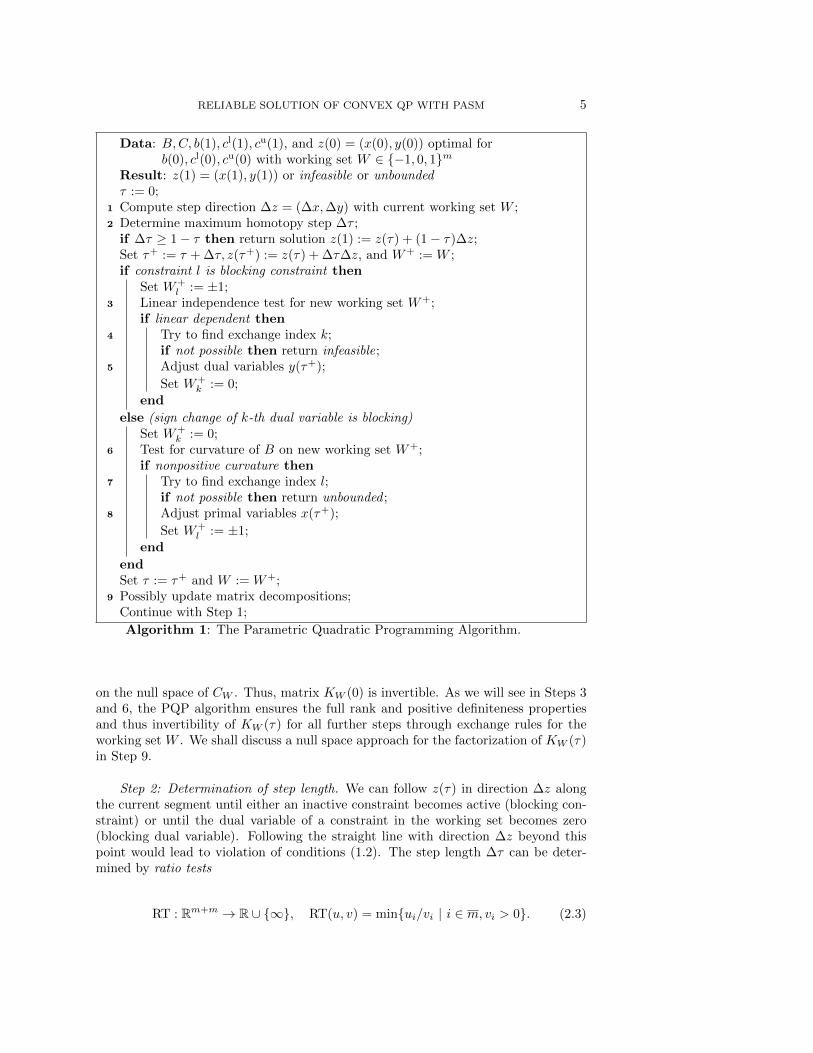
RELIABLE SOLUTION OF CONVEX QP WITH PASM 5
Data: B,C, b(1), cl(1), cu(1), and z(0) = (x(0), y(0)) optimal forb(0), cl(0), cu(0) with working set W ∈ {−1, 0, 1}m
Result: z(1) = (x(1), y(1)) or infeasible or unboundedτ := 0;Compute step direction ∆z = (∆x,∆y) with current working set W ;1
Determine maximum homotopy step ∆τ ;2
if ∆τ ≥ 1− τ then return solution z(1) := z(τ) + (1− τ)∆z;Set τ+ := τ + ∆τ, z(τ+) := z(τ) + ∆τ∆z, and W+ := W ;if constraint l is blocking constraint then
Set W+l := ±1;
Linear independence test for new working set W+;3
if linear dependent thenTry to find exchange index k;4
if not possible then return infeasible;Adjust dual variables y(τ+);5
Set W+k := 0;
end
else (sign change of k-th dual variable is blocking)Set W+
k := 0;Test for curvature of B on new working set W+;6
if nonpositive curvature thenTry to find exchange index l;7
if not possible then return unbounded ;Adjust primal variables x(τ+);8
Set W+l := ±1;
end
endSet τ := τ+ and W := W+;Possibly update matrix decompositions;9
Continue with Step 1;
Algorithm 1: The Parametric Quadratic Programming Algorithm.
on the null space of CW . Thus, matrix KW (0) is invertible. As we will see in Steps 3and 6, the PQP algorithm ensures the full rank and positive definiteness propertiesand thus invertibility of KW (τ) for all further steps through exchange rules for theworking set W . We shall discuss a null space approach for the factorization of KW (τ)in Step 9.
Step 2: Determination of step length. We can follow z(τ) in direction ∆z alongthe current segment until either an inactive constraint becomes active (blocking con-straint) or until the dual variable of a constraint in the working set becomes zero(blocking dual variable). Following the straight line with direction ∆z beyond thispoint would lead to violation of conditions (1.2). The step length ∆τ can be deter-mined by ratio tests
RT : Rm+m → R ∪ {∞}, RT(u, v) = min{ui/vi | i ∈ m, vi > 0}. (2.3)
6 A. POTSCHKA, C. KIRCHES, H. G. BOCK, AND J. P. SCHLODER
If the set of ratios is empty the minimum yields ∞ by convention. With the help ofRT, the maximum step towards the first blocking constraint is given by
tp = min{RT(Cx(τ)− cl,−C∆x),RT(cu − Cx(τ), C∆x)}, (2.4)
and towards the first blocking dual variable by
td = RT(W ◦ y(τ),W ◦∆y), (2.5)
where ◦ denotes elementwise multiplication to compensate for the opposite signs ofthe dual variables for lower and upper active constraints. The maximum step allowedis therefore
∆τ = min{tp, td}.
Best [3] assumes that all occuring minimizations yield either∞ or a unique minimizerwith corresponding index l ∈ m if ∆τ = tp or index k ∈ m if ∆τ = td from the setsof the ratio tests. The occurence of at least one nonunique minimizer is called a tie.We can distinguish between primal-dual ties if tp = td, primal ties if l is not unique,and dual ties if k is not unique. In case of a tie it is not clear which constraint shouldbe added or removed from the working set W and bad choices can lead to cycling oreven stalling of the method. Thus, successful treatment of ties is paramount to thereliability of Parametric Active Set methods and shall be further discussed in §4.3.
Step 3: Linear independence test. The addition of a new constraint l to theworking set W can lead to rank deficiency of CW+ and thus loss of invertibility ofmatrix KW (τ+). The linear dependence of Cl on Ci, i : Wi 6= 0 can be verified bysolving (
B CTW
CW 0
)(sξW
)=
(CTl
0
). (2.6)
Only if s = 0 then Cl is linearly dependent on Ci, i : Wi 6= 0 [3]. The linear indepen-dence test can be evaluated cheaply by reusing the factorization needed to solve thestep equation (2.2).
Step 4: Determination of exchange index k. It holds that s = 0. Let ξ beconstructed from ξW like ∆y from ∆yW . Equation (2.6) then yields
Cl =∑
i:Wi 6=0
ξiCi. (2.7)
Multiplying equation (2.7) by λW+l with λ ≥ 0 and adding this as a special form of
zero to the stationarity condition in equations (1.2) yields
B(x(τ) + ∆τ∆x)− b(τ+)
=∑
i:Wi 6=0
yi(τ+)CT
i = −λW+l C
Tl +
∑i:Wi 6=0
(yi(τ+) + λW+
l ξi)CTi . (2.8)
Thus, all coefficients of Ci, i : W+i 6= 0 on the right hand side of equation (2.8) are
also valid choices y for the dual variables as long as they satisfy the sign conditionW+i yi ≤ 0. Hence we can compute the largest such λ with the ratio test
λ = RT(−W+l (W ◦ y(τ+)),W+
l (W ◦ ξ)). (2.9)
If λ = ∞ then the parametric QP does not possess a feasible point beyond τ+ andthus the QP to be solved (at τ = 1) is infeasible. Otherwise, let k be a minimizingindex of the ratio set.
RELIABLE SOLUTION OF CONVEX QP WITH PASM 7
Step 5: Jump in dual variables. Now let
yi =
{−λW+
i for i = l,
yi(τ+) + λW+
i ξi for i : Wi 6= 0,
and set y(τ+) := y. It follows from construction of λ that yk = 0 and thus, constraintk can leave the working set. As a consequence, matrix CW+\{k} preserves the fullrank property and has the same null space as CW , thus securing regularity of matrixKW+(τ+).
Step 6: Curvature test. The removal of a constraint from the working set canlead to exposing directions of zero curvature on the null space of CW+ , which is largerthan the null space of CW , leading to singularity of matrix KW+(τ+). This can bedetected by solving (
B CTW
CW 0
)(sξW
)=
(0
−(ek)W
), (2.10)
where ek is the k-th column of the m-by-m identity matrix. Only if ξ = 0 then B issingular on the null space of CW+ [3]. As for the linear independence test of Step 3,the curvature test can be evaluated cheaply by reusing the factorization needed tosolve the step equation (2.2).
Step 7: Determination of exchange index l. It holds that ξ = 0 and s solves
Bs = 0, Cks = −1, CW+s = 0. (2.11)
Therefore all points x = x(τ+)+σs are also solutions if x is feasible. We can computethe largest such σ = min{σl, σu} with the ratio tests
σl = RT(Cx(τ+)− cl,−Cs), σu = RT(cu − Cx(τ+), Cs). (2.12)
If σ = ∞ then the parametric QP is unbounded beyond τ+, including the QP to besolved (at τ = 1). Otherwise, let l be a minimizing index of a ratio set which deliversa final minimizer of σ.
Step 8: Jump in primal variables. Now set x(τ+) := x(τ+)+σs. By constructionof σ we have that either Clx(τ+) = cll (if σ = σl) or Clx(τ+) = cul (otherwise). Thusl can be added to the working set via W+
l := −1 (if σ = σl) or W+l := +1.
Step 9: Update matrix decompositions. We summarize a null space approach forthe solution of systems (2.2), (2.6), and (2.10). A range space approach is in generalnot possible if B is only semidefinite [29]. A direct factorization of KW (τ) via LDLT
factorization is also possible [24] but update formulae are in the general case not asefficient as for the null space approach. The alternative of iterative linear algebramethods for the indefinite matrix KW (τ) are beyond the scope of this paper.
The null space approach is based on a QR decomposition of the transposed activeconstraint matrix
CTW = QR =
(Y Z
)(R0
)= Y R, QTQ = I.
Thus, the columns of Z constitute an orthonormal basis of the null space of CW .The columns of Y are an orthonormal basis of the range space of CT
W and the upper
8 A. POTSCHKA, C. KIRCHES, H. G. BOCK, AND J. P. SCHLODER
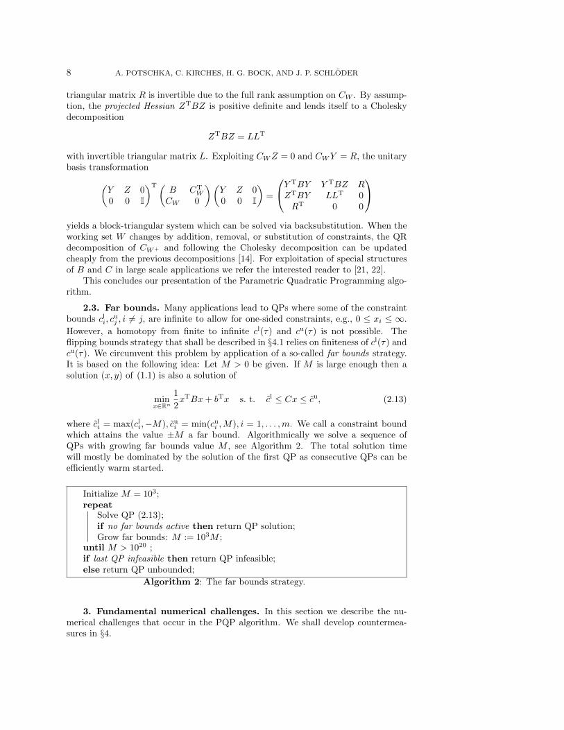
triangular matrix R is invertible due to the full rank assumption on CW . By assump-tion, the projected Hessian ZTBZ is positive definite and lends itself to a Choleskydecomposition
ZTBZ = LLT
with invertible triangular matrix L. Exploiting CWZ = 0 and CWY = R, the unitarybasis transformation(
Y Z 00 0 I
)T(B CT
W
CW 0
)(Y Z 00 0 I
)=
Y TBY Y TBZ RZTBY LLT 0RT 0 0
yields a block-triangular system which can be solved via backsubstitution. When theworking set W changes by addition, removal, or substitution of constraints, the QRdecomposition of CW+ and following the Cholesky decomposition can be updatedcheaply from the previous decompositions [14]. For exploitation of special structuresof B and C in large scale applications we refer the interested reader to [21, 22].
This concludes our presentation of the Parametric Quadratic Programming algo-rithm.
2.3. Far bounds. Many applications lead to QPs where some of the constraintbounds cli, c
uj , i 6= j, are infinite to allow for one-sided constraints, e.g., 0 ≤ xi ≤ ∞.
However, a homotopy from finite to infinite cl(τ) and cu(τ) is not possible. Theflipping bounds strategy that shall be described in §4.1 relies on finiteness of cl(τ) andcu(τ). We circumvent this problem by application of a so-called far bounds strategy.It is based on the following idea: Let M > 0 be given. If M is large enough then asolution (x, y) of (1.1) is also a solution of
minx∈Rn
1
2xTBx+ bTx s. t. cl ≤ Cx ≤ cu, (2.13)
where cli = max(cli,−M), cui = min(cui ,M), i = 1, . . . ,m. We call a constraint boundwhich attains the value ±M a far bound. Algorithmically we solve a sequence ofQPs with growing far bounds value M , see Algorithm 2. The total solution timewill mostly be dominated by the solution of the first QP as consecutive QPs can beefficiently warm started.
Initialize M = 103;repeat
Solve QP (2.13);if no far bounds active then return QP solution;Grow far bounds: M := 103M ;
until M > 1020 ;if last QP infeasible then return QP infeasible;else return QP unbounded;
Algorithm 2: The far bounds strategy.
3. Fundamental numerical challenges. In this section we describe the nu-merical challenges that occur in the PQP algorithm. We shall develop countermea-sures in §4.
RELIABLE SOLUTION OF CONVEX QP WITH PASM 9
One fundamental challenge in many applications is ill-posedness of problems:Small changes in the data of the problem lead to large changes in the solution. Thischallenge necessarily propagates through the algorithm and leads to ill-conditionedmatrices KW . As a consequence the results of the step computation (2.2), the lin-ear independence test (2.6), and the curvature test (2.10) can be errorneous up tocond(KW ) times machine precision in relative error [34]. This, in turn, can lead tovery instable ratio tests (2.3) and wrong choices for the working set which can causethe algorithm to break down.
Rounding errors can also accumulate over several iterations and lead to the para-metric “solution” z(τ) being optimal with an accuracy much less than machine preci-sion. This phenomenon is called drift. Large drift can also lead to breakdown of thealgorithm because the general assumption of optimality of z(τ) is violated.
Furthermore, the termination criterion must also be adapted to work reliably onboth well- and ill-conditioned problems.
Ill-conditioning can also be introduced if the null space of CW captures two eigen-values of B with high ratio, leading to ill-conditioning of the Cholesky factors L. Inthe extreme case, the next step for the dual variables can be afflicted with a largeerror, causing again instability in the ratio tests.
The second fundamental challenge is the occurence of comparisons with zero,a delicate subject in the presence of rounding errors. These comparisons permeatethe algorithm from the sign condition in the ratio tests (2.3) to the tests for lineardependence (2.6) or zero curvature (2.10).
The third fundamental challenge is the treatment of ties, i.e., nonuniqueness ofminimizers of the ratio tests (2.3). Consider the case mentioned in §2.1 of a homo-topy starting at x(0) = 0, y(0) = 0, b(0) = 0, cl(0) = 0, cu(0) = 0,W = 0. Clearly(x(0), y(0)) is an optimal solution at τ = 0 regardless of the choice of B and C. Notethat for the PQP algorithm the choice of W = 0 is only possible if B is positive defi-nite. The first step direction will then point towards the unconstrained minimizer ofthe objective. If more than one constraint is active in the solution at τ = 1 then theprimal ratio test (2.4) for determination of the step length yields a (multiple) primaltie with ∆τ = tp = 0. Of all possible ratio test minimizers, one has to be chosen.One approach seems to be to employ pricing heuristics from primal/dual Active Setmethods but we prefer a different approach which we discuss in §4.3. In the followingiterations, primal-dual ties can occur while still ∆τ = 0. Thus cycling, the repeatedaddition and removal of the same constraints without any progress, can be possiblewhich leads to stalling of the method. We are not aware of any pricing strategy whichcan avoid the problem of cycling. Ties also occur naturally in the case of degenerateQPs, where the optimal primal or dual variables are not uniquely determined.
4. Strategies to meet numerical challenges. We propose to employ thefollowing strategies for Parametric Active Set methods to meet the fundamental nu-merical challenges described in §3.
4.1. Rounding errors and ill-conditioning. The most effective countermea-sure against the challenges of ill-conditioning is to iteratively improve the quality ofthe linear system solutions via
Iterative Refinement [34]. We have already mentioned that the relative error inthe solution z of
KW z = d
10 A. POTSCHKA, C. KIRCHES, H. G. BOCK, AND J. P. SCHLODER
can be as high as cond(KW ) times machine precision. Thus, if cond(KW ) ≈ 1010 andwe perform computations in double precision, the solution z can have as little as sixvalid decimal digits. Iterative Refinement
z0 = 0, rk = KW zk − d, KW δz
k = rk, zk+1 = zk − δzk
recovers a fixed number of extra valid digits in each iteration. In the previous example,the iterate z2 has at least twelve valid decimal digits after only one extra step ofIterative Refinement. It is worth noticing that compared to the original “solution”z1 each iteration only needs to perform one additional matrix-vector-multiplicationwith KW and one backwards solve with the decomposition of KW described in §2.2.In exact arithmetic zk+1 = zk for all k ≥ 1.
Drift correction. A very effective strategy to avoid drift can be formulated if thePQP algorithm is cast in a slightly different framework. After each iteration, werescale the homotopy parameter to τ = 0, thus interpreting the iterate z(τ+) as anew starting value z(0). This does not avoid drift yet but allows for modifications torestore consistency of the starting point via
cli(0) :=
{Cix(0) if Wi = −1,
min{cli(0), Cix(0)} otherwise,
cui (0) :=
{Cix(0) if Wi = +1,
max{cui (0), Cix(0)} otherwise,
yi(0) :=
max{0, yi(0)} if Wi = −1,
min{0, yi(0)} if Wi = +1,
0, otherwise,
b(0) := Bx(0)− CTy(0),
for i ∈ m. This annihilates the effects of drift after every iteration, at the cost ofsplitting up the single homotopy into a sequence of homotopies which are, however,very close to the remaining part of the original homotopy. In exact arithmetic theproposed modification does not alter any value.
Termination Criterion. It is tempting to use the homotopy parameter τ in thetermination criterion as proposed in Algorithm 1. However, this choice renders thetermination criterion dependent on the choice of the homotopy start, an undesirableproperty. Instead, we propose to use the relative distance δ in the data space
∆0 = (b(τ), cl(τ), cu(τ)), sj = (∆1j −∆0
j )/max{1, |∆1j |}, j = 1, . . . , n+m+m,
∆1 = (b(1), cl(1), cu(1)), δ = ‖s‖∞.
This choice renders the termination criterion independent of the condition numberof KW (1). We observe that the termination criterion can give no guarantee for thedistance to the exact solution. Instead, a backwards analysis result holds: The com-puted solution is the exact solution to a problem which is as close as δ to the oneto be solved. The numerical results presented in §6 were obtained with the toleranceδ ≤ δterm = 1e7 eps.
Ill-conditioning of the Cholesky factors L. To avoid ill-conditioning of the Choleskyfactors L we have developed the so-called flipping bounds strategy. Flipping boundsis similar to taking long steps in the dual Simplex method [23, 30], where one variable
RELIABLE SOLUTION OF CONVEX QP WITH PASM 11
changes in the working set from upper to lower bound immediately without becominginactive in between, i.e., it flips. Flipping is only possible if cl(1) and cu(1) haveonly finite entries, which is guaranteed by the far bounds strategy described in §2.3.We modify the PQP algorithm in the following way: If a constraint l was removedwithout requiring another constraint k to enter the active set, we monitor the size ofthe smallest entry `i of the diagonal of L in Step 9. If `2i < δcurv we have detecteda small eigenvalue in L which corresponds to a small eigenvalue of B now uncoveredthrough the removal of constraint l. To avoid ill-conditioning of LLT, we introduce ajump in the QP homotopy by requiring that the other bound of constraint l is movedsuch that it becomes active immediately (hence the name flipping bounds) throughsetting
cll(τ+) := cul (τ+),W+
l = −1, if Wl = +1,
cul (τ+) := cll(τ+),W+
l = +1, if Wl = −1.
The entries j 6= l of cl and cu are set to the corresponding entries of cl and cu.Consequently the Cholesky decomposition from the previous step stays valid for thecurrent projected Hessian.
The numerical results presented in §6 were obtained with the curvature toleranceδcurv = 1e4 eps.
4.2. Comparison with zero.
Ratio tests. In the ideal ratio test (2.3) we take a minimum over a subset of mquotients with strictly positive denominator. The presence of round-off error makes itnecessary to substitute the ideal ratio test by an expression with adjustable tolerances,e.g.,
ucuti = max(ui, εcut), i ∈ m,RTr(u, v, εcut, εden, εnum) = min{ucuti /vi | i ∈ m, vi ≥ εden, ucuti ≥ εnum}.
We now explain the purpose of the three tolerances: The denominator tolerance εden >0 describes which small but positive values of vi should already be considered less thanor equal to zero. They are consequently discarded as candidates for the minimum.
The cutting tolerance εcut and the numerator tolerance εnum offer the freedom oftwo different treatments for numerators close to zero. If εcut > εnum then negativenumerators are simply cut off at εcut before the quotients are taken, yielding that theminimum is greater or equal to εcut/εden. For instance, we set εcut = 0 in the ratiotests for determination of the step length (2.4) and (2.5). This choice is motivated bythe fact that in exact arithmetic ui ≥ 0 for all i ∈ m with vi > 0. Thus, only valuesui which are negative due to round-off are manipulated and the step length satisfies∆τ ≥ 0 also in finite precision arithmetic.
If εcut ≤ εnum then cutting does not have any effect. We have found it beneficialfor the reliability of PASM to set εnum = εden in the ratio tests (2.9) and (2.12) forfinding exchange indices.
The numerical results presented in §6 were obtained with the ratio test tolerancesεden = −εnum = 1e3 eps and εcut = 0 for step length determination and εden = εnum =−εcut = 1e3 eps for the remaining ratio tests.
Linear independence and zero curvature test. After solution of systems (2.6)and (2.10) for s and ξW we must compare the norm of s or ξ with zero. Let ζ = (s, ξ).
12 A. POTSCHKA, C. KIRCHES, H. G. BOCK, AND J. P. SCHLODER
We propose to use the relative conditions
‖s‖∞ ≤ εtest‖ζ‖∞ for the linear dependence test and (4.1)
‖ξ‖∞ ≤ εtest‖ζ‖∞ for the zero curvature test. (4.2)
We remark that ‖ζ‖∞ = ‖ξ‖∞ if s = 0 and ‖ζ‖∞ = ‖s‖∞ if ξ = 0. Thus we canreplace ‖ζ‖∞ in the code by ‖ξ‖∞ in test (4.1) and by ‖s‖∞ in test (4.2).
The numerical results presented in §6 were obtained with εtest = 1e5 eps.
4.3. Cycling and ties. Once ties have occured, their resolution is a costlyaffair because of the combinatorial nature of the decision which subset of the possibleconstraints should be chosen to leave or enter the working set. This decision can bebased on the solution of yet another QP of larger size then the original problem [33]or on heuristics similar to anti-cycling rules in the Simplex method.
We prefer a different approach instead. The idea behind the strategy we proposefor ties is simple: Instead of trying to treat ties, we try to avoid them in the first place.The strategy is as simple as the idea and exploits the homotopy framework of PASM.Let a homotopy start b(0), cl(0), cu(0) with optimal solution (x(0), y(0)) and workingset W be given. Then, for every triple of m-vectors r0, r1, r2 ≥ 0, the primal-dualpair (x(0), y(0)) with
yi(0) =
yi(0) + ri if Wi = −1,
yi(0) if Wi = 0,
yi(0)− ri if Wi = +1,
i ∈ m,
is an optimal solution to the homotopy start b(0), cl(0), cu(0), where for i ∈ m
cli(0) =
{cli(0), if Wi = −1,
cli(0)− r1i , otherwise,
cui (0) =
{cui (0), if Wi = +1,
cui (0) + r2i , otherwise,
b(0) = −(Bx(0)− CTy(0)).
In other words, if we move the inactive constraint bounds further away from Cx(0)and the dual variables of the active constraints further away from zero, x(0) staysfeasible and b(0) can be adapted to restore optimality of (x(0), y(0)) with the sameworking set W . Recall that the ratio tests depend exactly on the residuals of theinactive constraints and the dual variables of the active constraints. In our numericaltests, the simple choice of
rji = (1 + (i− 1)/(m− 1))/2, j = 0, 1, 2, i ∈ m,
has proven to work reliably. Because of the shape of rj , we call this strategy ramping.It is important to avoid two entries of rj to have the same value because manyproblems have special structures, e.g., variable bounds of the same value for severalvariables which lead to primal ties if the homotopy starts with the same value for eachof these variables. Of course, the choice of linear ramping is somewhat arbitrary andif a problem happens to have variable bounds in the form of a ramp, ties are againpossible. However, this kind of structure is much less common than equal variablebounds.
RELIABLE SOLUTION OF CONVEX QP WITH PASM 13
We employ ramping in the starting point of the homotopy and also after aniteration which resulted in a zero step ∆τ = 0. Of course, this can lead to largejumps in the problem homotopy and practically catapult the current b(0) := b(0)away from b(1). However, a PASM is capable of reducing even a large distance in thedata space to zero in one step, provided the active set is right. Thus, the distance ofthe working set W to the active set of the solution is a more appropriate measure ofthe progress of a PASM. By construction, the active set is preserved by the rampingstrategy.
We further want to remark that ties can never be completely avoided. For instancein case of a QP whose solution lies in a degenerate corner, a tie must occur in (atleast) one iteration of a PASM. In the numerical examples we have treated so far, theramping strategy effectively deferred these ties to the final step, where a tie is not aproblem any more because the solution at the end of the last homotopy segment isalready one of infinitely many solutions of the QP to be solved and no ties must beresolved in the solution.
5. The code rpasm: A PASM in Matlab R©. We have implemented thestrategies proposed in §4 in a Matlab R© code called rpasm. The main purpose of thecode is to demonstrate reliability and solution quality on the test set. In favor of codesimplicity we have refrained from employing special structure exploiting linear algebraroutines which could greatly enhance the runtime of the code. The three main fea-tures in the C++ PASM code qpOASES [9, 10] for runtime improvement in the linearalgebra routines are special treatment of variable bounds, updates for QR decompo-sitions, and appropriate updates for Cholesky decompositions. Of the three, rpasmonly performs QR updates. Variable bounds are simply treated as general inequalityconstraints. Cholesky decompositions are computed from scratch after a change inthe active set. Furthermore, only dense linear algebra routines are used which donot exploit the often sparse matrices in the test examples. Another feature which iscommon in most commercial QP solvers is the use of a preprocessing/presolve stepto reduce the problem size by eliminating fixed variables and dispensable constraintsand possibly scaling the data. We will see that rpasm works reliably even withoutpreprocessing.
The merging of the features of qpOASES and rpasm exceeds the aim of this paperand will be presented in a future publication.
6. Comparison with existing software. From the codes contained in Ta-ble 1.1 we use the ones which are freely available for academic purposes and comewith a Matlab R© interface, i.e., CPLEX, OOQP, qpOASES, plus the Matlab R© solverquadprog and the newly developed rpasm. The programs cover the range of Pri-mal Active Set (CPLEXP, quadprog), Dual Active Set (CPLEXD), Barrier/InteriorPoint (CPLEXB, OOQP), and Parametric Active Set (qpOASES, rpasm). For rpasm,we further differentiate between a version without iterative refinement (rpasm0) andwith one possible step of iterative refinement (rpasm1). All codes were used withtheir default settings on all problems.
6.1. Criteria for comparison. We compare the runtime and the quality of thesolution. Runtime was measured as the average runtime of three runs on one coreof a Intel R© CoreTM i7 with 2.67 GHz and 8 MB cache in Matlab R© 7.6 under Linux2.6 (64 bit). The quality of solutions (x∗, y∗) was measured using a residual ρ of
14 A. POTSCHKA, C. KIRCHES, H. G. BOCK, AND J. P. SCHLODER
conditions (1.2) defined via
ρstat = ‖Bx∗ + b− CTy∗‖∞, ρlcmpl = max{|(Cx∗ − cl)iy∗i | | y∗i ≥ +10 eps},ρfeas = max(0, cl − Cx∗, Cx∗ − cu), ρucmpl = max{|(Cx∗ − cu)iy
∗i | | y∗i ≤ −10 eps},
ρ = max(ρstat, ρfeas, ρlcmpl, ρ
ucmpl).
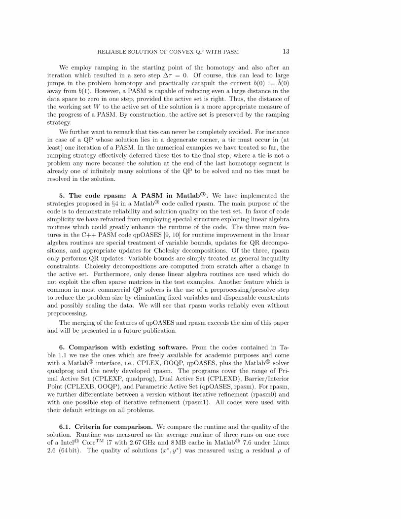
In Table 8.1 we have assembled the results for problems from the Maros-Meszarostest set [25] with at most n = 1000 variables and m = 1001 two-sided inequalityconstraints (not counting variable bound constraints). We have visualized the resultsin the performance graphs of Figures 6.1 and 6.2. The graphs display a time factor onthe abscissa versus the percentage of problems that each code was able to solve withinthe time factor times the runtime of the fastest method for each problem. Roughlyspeaking, the graph of a fast method is close to the left hand side of the diagram, thegraph of a reliable method is close to the top of the diagram.
Time factor
Percentageofproblemssolved
rpasm0rpasm1quadprogOOQPqpOASESCPLEXPCPLEXDCPLEXB
100 101 102 103 104 1050
10
20
30
40
50
60
70
80
90
100
Fig. 6.1. Performance comparison with loose residual threshold ρ ≤ 1e-2.
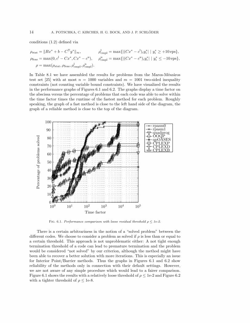
There is a certain arbitrariness in the notion of a “solved problem” between thedifferent codes. We choose to consider a problem as solved if ρ is less than or equal toa certain threshold. This approach is not unproblematic either: A not tight enoughtermination threshold of a code can lead to premature termination and the problemwould be considered “not solved” by our criterion, although the method might havebeen able to recover a better solution with more iterations. This is especially an issuefor Interior Point/Barrier methods. Thus the graphs in Figures 6.1 and 6.2 showreliability of the methods only in connection with their default settings. However,we are not aware of any simple procedure which would lead to a fairer comparison.Figure 6.1 shows the results with a relatively loose threshold of ρ ≤ 1e-2 and Figure 6.2with a tighter threshold of ρ ≤ 1e-8.
RELIABLE SOLUTION OF CONVEX QP WITH PASM 15
Time factor
Percentageofproblemssolved
rpasm0rpasm1quadprogOOQPqpOASESCPLEXPCPLEXDCPLEXB
100 101 102 103 104 1050
10
20
30
40
50
60
70
80
90
100
Fig. 6.2. Performance comparison with tight residual threshold ρ ≤ 1e-8.
6.2. Discussion of numerical results. We first discuss the results depictedin Figure 6.1 and continue with the differences to the tighter residual tolerance inFigure 6.2.
From Figure 6.1 we see that the newly developed code rpasm with iterative re-finement is the only code which solves all of the problems to the prescribed accuracy.It actually solves all of them to a residual of ρ ≤ 5e-5, as can be seen from Table 8.1.The version of rpasm without iterative refinement fails on three problems (95 %).Furthermore, both versions of rpasm dominate quadprog both in runtime and thenumber of solved problems (62 %). The primal and dual versions of CPLEX are thesecond most reliable with 96 % and 97 %. As can be seen from Table 8.1, CPLEXsolves no problem in less than 1.3 s, not even the small examples which are solvedin a few miliseconds by rpasm. We suspect that this is due to a calling overheadin CPLEX, e.g., for license checking. This is also one reason why OOQP is muchfaster than the Barrier version of CPLEX, although they both solve roughly the samenumber of problems (70 % and 73 %, respectively). Although the code qpOASES isonly appropriate for QPs with positive definite Hessian, which make up only 27 % ofthe considered problems, it still solves 44 % of the test problems. Additionally, wewant to stress that those problems solved by qpOASES were indeed solved quickly.
Now we discuss the differences between Figure 6.2 and Figure 6.1, i.e., whenswitching to a tighter residual tolerance of ρ ≤ 1e-8: The ratio of solved problemsdrops dramatically for the Interior Point/Barrier methods (CPLEXB: 29 %, OOQP:37 %). This is a known fact and the reason for the existence of crossover methodswhich refine the results of Interior Point/Barrier methods with an Active Set method.The code qpOASES still solves 44 % of the problems, which indicates that the solutionsthat qpOASES yields are of high quality. Furthermore, qpOASES is fast: It solves36 % of the problems within 110 % of the time of the fastest method for each of these
16 A. POTSCHKA, C. KIRCHES, H. G. BOCK, AND J. P. SCHLODER
problems. The number of problems solved by quadprog decreases to 53 %. The primaland dual Active Set versions of CPLEX solve 78 % of the problems. Only the coderpasm is able to solve more than 80 % of the problems to a residual of ρ ≤ 1e-8(rpasm0: 82 %, rpasm1: 84 %).
We can conclude that the strategies proposed in §4 indeed lead to a reliablemethod for the solution of convex QPs.
7. Drawbacks of the proposed PASM. Although the method has proved towork successfully on the test set, the improvement in reliability is acheived only atthe price of breaking the pure homotopy paradigm which complicates an otherwisestraightforward proof of convergence for the method: Drift correction, ramping, andthe flipping bounds strategy lead to jumps in the trajectories of b(τ), cl(τ), and cu(τ)and thus to a sequence of (possibly nonphysical) homotopies. Proving the nonex-istence or possibility of cycles through these strategies is beyond the scope of thispaper.
One major area of application for the code qpOASES is online feedback control [9,10]. Exploitation of the physical homotopy between two consecutive problems in timehas proven to be of advantage in this case. The proposed strategies should thus beused with care in this application field.
8. Nonconvex Quadratic Programs. The flipping bounds strategy presentedin §4.1 can also be extended to the case of nonconvex QPs with indefinite Hessianmatrix B. When the Cholesky factorization or update breaks down due to a negativediagonal entry, we also flip instead of remove the constraint l. Hence the projectedHessian always stays positive definite. By the second order necessary optimalitycondition, the projected Hessian in every isolated local minimum of the nonconvexQP is guaranteed to be positive definite. Conversely, if strict complementarity holdsat τ = 1 we obtain a local minimum because the second order sufficient condition issatisfied. No guarantees can be given in the case of violation of strict complementarity.
Finding a global minimum of a nonconvex QP is known to be an NP-hard problem,even if the Hessian has only one single negative eigenvalue [28]. However, a localsolution returned by the PASM can be refined by flipping all combinations of activebounds whose removal would lead to an indefinite projected Hessian and restartingthe PASM for each of these flipped Active Sets, revealing again the combinatorialnature of finding the global solution of the nonconvex QP.
In the context of SQP with indefinite Hessian approximations (e.g., symmetricrank one updates, the exact Hessian, etc.), a local solution of a nonconvex QP issufficient because the SQP method can only find local minima anyway.
For proof of concept we seek a local solution of the nonconvex problem
min1
2
k−2∑i=1
(xk+i+1 − xk+i)2 −1
2
k=1∑i=1
(xk−i + xk+i + αk−i+1)2 (8.1a)
s. t. xk+i − xi+1 + xi = 0, i = 1, . . . , k − 1, (8.1b)
αi ≤ xi ≤ αi+1, i = 1, . . . , k, (8.1c)
0.4(αi+2 − αi) ≤ xk+i ≤ 0.6(αi+2 − αi), i = 1, . . . , k − 1, (8.1d)
with given constants αi = 1 + 1.01i, i = 1, . . . , k − 1. We have adapted problem (8.1)from problem class 3 in Gould [16] by switching the sign in front of the second sumand the α terms in the objective. We start the computation with an initial guess ofx(0) = 0, y(0) = 0, set the lower bounds of equations (8.1c) and (8.1d) active in the
RELIABLE SOLUTION OF CONVEX QP WITH PASM 17
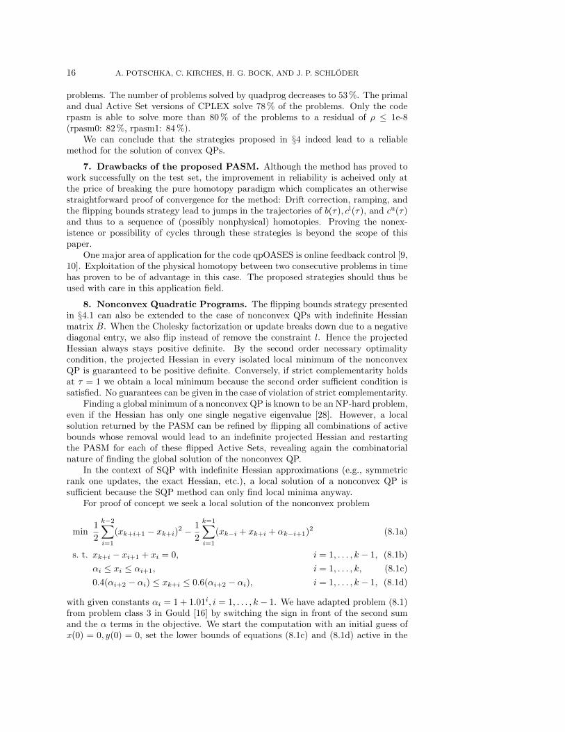
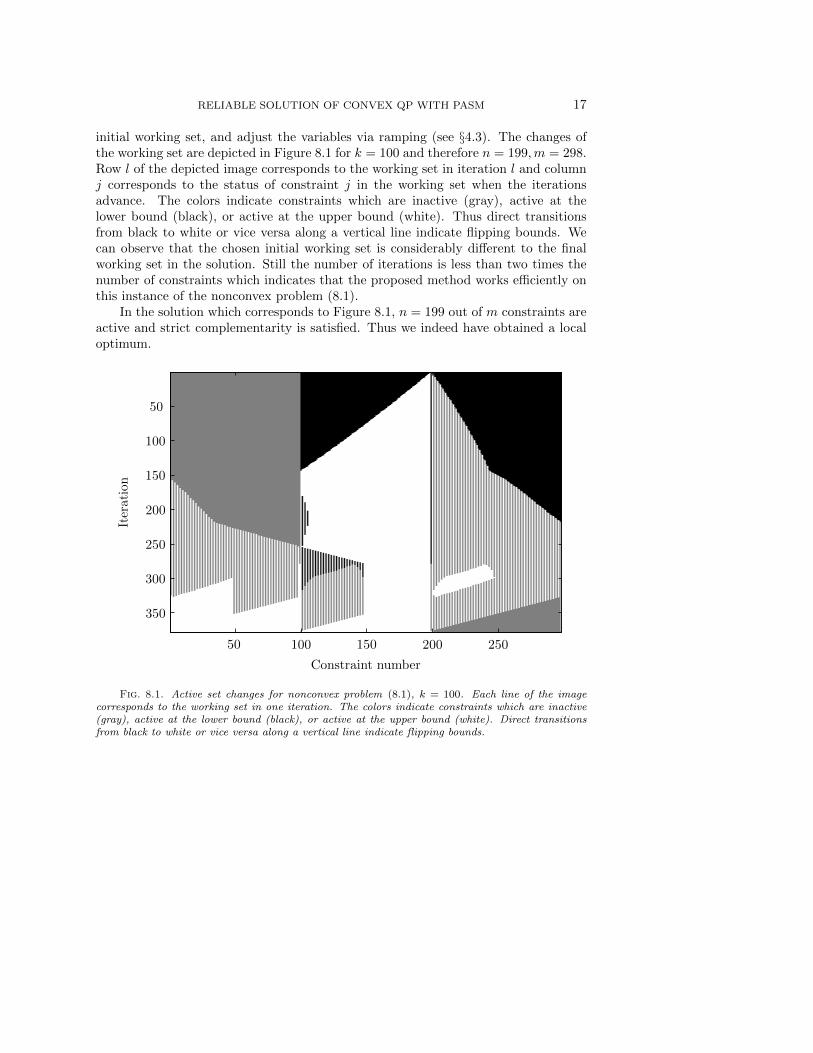
initial working set, and adjust the variables via ramping (see §4.3). The changes ofthe working set are depicted in Figure 8.1 for k = 100 and therefore n = 199,m = 298.Row l of the depicted image corresponds to the working set in iteration l and columnj corresponds to the status of constraint j in the working set when the iterationsadvance. The colors indicate constraints which are inactive (gray), active at thelower bound (black), or active at the upper bound (white). Thus direct transitionsfrom black to white or vice versa along a vertical line indicate flipping bounds. Wecan observe that the chosen initial working set is considerably different to the finalworking set in the solution. Still the number of iterations is less than two times thenumber of constraints which indicates that the proposed method works efficiently onthis instance of the nonconvex problem (8.1).
In the solution which corresponds to Figure 8.1, n = 199 out of m constraints areactive and strict complementarity is satisfied. Thus we indeed have obtained a localoptimum.
Constraint number
Iteration
50 100 150 200 250
50
100
150
200
250
300
350
Fig. 8.1. Active set changes for nonconvex problem (8.1), k = 100. Each line of the imagecorresponds to the working set in one iteration. The colors indicate constraints which are inactive(gray), active at the lower bound (black), or active at the upper bound (white). Direct transitionsfrom black to white or vice versa along a vertical line indicate flipping bounds.

18 A. POTSCHKA, C. KIRCHES, H. G. BOCK, AND J. P. SCHLODERproble
mrpasm
0rpasm
1quadprog
OO
QP
qpOASES
CPLEXP
CPLEXD
CPLEXB
nam
em
ntim
eρ
tim
eρ
tim
eρ
tim
eρ
tim
eρ
tim
eρ
tim
eρ
tim
eρ
CVXQ
P1
M500
1000
407.3
44
4e-1
0529.0
85
2e-0
875.7
50
5e-1
03.1
97
6e-0
66e+
00
1.7
57
2e-0
52.3
45
2e-0
62.0
96
3e-0
3CVXQ
P1
S50
100
0.5
76
5e-1
10.6
35
2e-1
10.1
14
2e-1
20.0
07
1e-0
86e+
00
1.5
75
2e-1
11.6
00
2e-1
11.6
30
1e-0
6CVXQ
P2
M250
1000
221.0
06
5e-1
2296.2
80
2e-1
1331.5
69
2e-1
11.6
42
2e-0
66e+
00
1.7
34
2e-0
71.8
34
2e-0
71.9
55
1e-0
4CVXQ
P2
S25
100
0.4
94
9e-1
30.5
40
2e-1
30.2
42
5e-1
30.0
06
4e-1
10.0
18
6e-1
31.6
63
5e-1
11.6
69
5e-1
11.6
32
2e-0
6CVXQ
P3
M750
1000
785.4
29
1e-0
9968.9
48
2e-0
830.0
66
1e-0
85.1
25
4e-0
86e+
00
1.8
39
5e-0
93.0
86
2e-0
92.5
76
3e-0
2CVXQ
P3
S75
100
0.6
84
5e-1
10.7
55
7e-1
10.0
51
1e-1
20.0
12
2e-1
06e+
00
1.5
29
2e-1
21.5
30
5e-1
31.5
64
3e-0
6D
PK
LO
177
133
2.2
64
1e-1
42.4
72
1e-1
40.0
17
3e-1
40.0
10
4e-1
50.0
13
6e-1
41.5
23
3e-1
41.5
23
2e-1
41.5
31
3e-1
4D
UAL1
185
0.2
55
3e-1
50.2
98
2e-1
50.0
86
2e-1
50.0
03
2e-0
80.0
15
8e-1
51.5
26
2e-1
51.5
34
2e-1
51.5
50
1e-0
9D
UAL2
196
0.3
19
2e-1
50.3
50
1e-1
50.0
28
2e-1
50.0
03
2e-0
70.0
22
3e-1
51.5
66
2e-1
51.5
14
2e-1
51.5
81
2e-1
0D
UAL3
1111
0.4
37
2e-1
50.4
69
3e-1
50.0
75
2e-1
50.0
03
4e-0
70.0
23
4e-1
51.5
32
3e-1
51.5
38
3e-1
51.5
54
1e-0
9D
UAL4
175
0.1
82
2e-1
50.1
96
2e-1
50.0
46
2e-1
50.0
02
4e-0
70.0
04
6e-1
51.5
62
1e-1
41.5
33
1e-1
41.5
84
4e-0
9D
UALC1
215
90.0
07
4e-1
20.0
08
6e-1
10.0
18
9e-1
00.0
36
2e-0
70.0
01
5e-1
21.5
31
1e-1
01.5
46
1e-1
01.5
51
2e-0
6D
UALC2
229
70.0
06
2e-1
20.0
07
2e-1
20.0
15
6e-1
10.0
42
3e-1
10.0
00
4e-1
21.5
46
5e-1
21.5
18
5e-1
21.5
52
7e-0
7D
UALC5
278
80.0
08
7e-1
30.0
08
3e-1
30.0
13
5e-1
30.0
56
7e-0
80.0
01
9e-1
31.5
44
2e-1
21.5
39
2e-1
21.5
56
4e-0
8D
UALC8
503
80.0
07
5e-1
10.0
09
1e-0
50.0
19
1e-1
00.2
82
7e-1
00.0
01
4e-1
11.5
51
1e-1
01.5
40
1e-1
01.5
60
7e-0
7G
ENHS28
810
0.0
20
4e-1
60.0
21
4e-1
60.0
10
1e-1
50.0
00
1e-1
60.0
00
4e-1
61.5
28
2e-1
61.5
38
3e-1
51.5
66
2e-1
6G
OULD
QP2
349
699
635.7
13
3e-0
9721.6
74
3e-0
980.2
82
7e-1
40.6
44
2e-0
73e+
01
1.6
96
5e-0
71.5
81
9e-0
71.5
71
2e-0
8G
OULD
QP3
349
699
87.9
67
7e-1
5110.3
01
7e-1
520.1
75
6e-1
41.4
27
4e-0
77.5
75
2e-1
31.5
81
1e-1
41.5
32
2e-1
41.5
23
2e-0
6HS118
17
15
0.0
39
2e-1
50.0
41
3e-1
40.0
24
1e-1
30.0
02
3e-1
30.0
01
1e-1
31.5
24
2e-1
61.5
04
2e-1
61.5
28
3e-0
8HS21
12
0.0
02
1e-1
60.0
02
2e-1
70.0
10
0e+
00
0.0
01
2e-1
20.0
00
0e+
00
1.5
12
0e+
00
1.4
97
0e+
00
1.5
19
6e-1
0HS268
55
0.0
10
1e-1
10.0
10
1e-0
60.0
11
7e-1
20e+
00
0.0
00
1e-1
11.5
26
2e-1
11.5
21
2e-1
12e+
10
HS35
13
0.0
04
0e+
00
0.0
04
9e-1
60.0
10
4e-1
60.0
01
2e-1
50.0
00
5e-1
51.5
35
0e+
00
1.5
37
0e+
00
1.5
29
2e-0
8HS35M
OD
13
0.0
05
5e-1
50.0
05
0e+
00
0.0
10
0e+
00
0.0
01
1e+
00
0.0
00
0e+
00
1.5
09
0e+
00
1.5
22
0e+
00
1.5
25
2e-0
8HS51
35
0.0
06
5e-1
50.0
07
9e-1
60.0
10
9e-1
60.0
00
2e-3
20.0
00
4e-1
61.5
40
0e+
00
1.5
04
0e+
00
1.5
44
0e+
00
HS52
35
0.0
10
2e-1
50.0
11
5e-1
60.0
09
2e-1
50.0
00
2e-1
60.0
00
2e-1
51.5
26
5e-1
51.5
47
8e-1
51.5
30
9e-1
6HS53
35
0.0
10
9e-1
60.0
10
2e-1
50.0
15
2e-1
50.0
01
2e-0
80.0
00
9e-1
61.5
19
0e+
00
1.5
42
0e+
00
1.5
16
2e-1
0HS76
34
0.0
04
2e-1
60.0
04
1e-1
60.0
11
2e-1
60.0
01
1e-1
30.0
00
5e-1
41.5
09
0e+
00
1.5
08
0e+
00
1.5
30
7e-0
9K
SIP
1001
20
1.7
18
2e-1
61.8
89
3e-1
60.2
48
2e-1
64.4
91
1e-0
81e+
00
1.7
42
6e-1
61.5
87
1e-1
68.6
89
1e-0
9LO
TSCHD
712
0.0
23
9e-1
40.0
23
4e-1
30.0
13
1e-1
20.0
01
2e-0
71e+
02
1.5
68
2e-1
31.5
91
2e-1
31.5
96
2e-0
6M
OSARQ
P2
600
900
359.3
03
4e-1
5399.6
30
4e-1
5697.5
50
2e+
00
13.3
43
4e-0
713.9
42
3e-1
31.6
92
5e-1
41.5
55
7e-1
41.6
99
2e-0
6PRIM
AL1
85
325
14.9
51
1e-1
616.0
26
7e-1
72.2
32
4e-1
60.3
75
9e-0
80.5
73
6e-1
41.5
48
3e-1
41.5
13
3e-1
41.5
80
6e-1
0PRIM
AL2
96
649
156.4
41
2e-1
5166.7
42
4e-1
618.0
18
4e-1
61.8
72
6e-0
79.8
32
2e-1
31.5
95
7e-1
51.5
52
7e-1
51.6
08
1e-1
0PRIM
AL3
111
745
255.5
30
4e-1
6282.3
54
3e-1
627.5
84
1e-1
52.5
52
1e-0
615.1
90
3e-1
31.8
01
5e-1
41.5
87
5e-1
41.7
19
2e-0
9PRIM
ALC1
9230
0.4
30
3e-1
20.5
08
9e-1
31.8
77
1e-0
80.0
91
2e-1
10.0
22
1e-1
11.4
92
4e-1
21.4
80
2e-1
21.4
96
6e-0
8PRIM
ALC2
7231
0.2
09
2e-1
20.2
46
5e-1
31.9
76
2e-0
80.0
94
3e-1
00.0
21
8e-1
31.4
77
6e-1
21.4
83
6e-1
21.4
94
3e-0
8PRIM
ALC5
8287
0.2
85
2e-1
30.3
69
2e-1
33.6
03
2e-0
90.1
46
7e-1
00.0
41
2e-1
31.4
72
2e-1
31.5
16
1e-1
21.5
48
5e-0
8PRIM
ALC8
8520
2.1
13
1e-1
13.0
34
7e-1
226.5
85
4e-0
60.5
99
1e-1
10.3
33
4e-1
11.4
71
2e-1
01.4
64
3e-1
01.4
52
2e-0
5Q
AD
LIT
TL
56
97
0.4
93
1e-0
90.5
17
8e-1
00.9
86
1e+
02
9e+
43
3e+
03
1.4
14
7e-1
11.4
21
7e-1
11.4
33
9e-0
7Q
AFIR
O27
32
0.0
26
1e-1
40.0
29
9e-1
61e+
01
0.0
03
3e-0
94e+
01
1.4
40
1e-1
41.4
48
1e-1
41.5
30
2e-1
0Q
BAND
M305
472
71.0
53
2e-1
399.4
55
5e-1
24e+
02
7e+
12
7e+
01
1.5
06
6e-1
31.5
15
6e-1
31.5
36
1e-0
6Q
BEACO
NF
173
262
2.2
08
3e-1
12.5
94
4e-1
12e+
03
8e+
20
2e+
03
1.5
11
3e-1
11.5
15
3e-1
15e+
20
QBO
RE3D
233
315
4.1
48
9e-0
94.9
99
3e-0
93e+
02
1e+
40
3e+
02
1.3
93
9e-1
31.3
92
5e-1
31.4
08
2e-0
6Q
BRANDY
220
249
10.5
88
8e-1
113.2
25
1e-1
09e+
02
0e+
00
8e+
01
1.3
86
4e-1
21.3
86
8e-1
27e+
02
QCAPRI
271
353
27.5
99
1e-0
831.5
82
1e-0
84e+
04
9e+
19
3e+
03
1.3
96
1e-0
81.3
97
1e-0
86e+
20
QE226
223
282
14.4
47
5e-1
318.5
29
9e-1
42e+
03
1e+
20
3e+
01
1.4
16
1e-1
31.4
20
1e-1
31e+
20
QETAM
ACR
400
688
136.0
91
5e-0
5181.1
63
5e-0
59e+
02
8e+
11
8e+
02
9e+
02
1.5
07
1e-0
71.5
65
2e-0
5Q
FFFFF80
524
854
2e+
05
1351.8
14
4e-0
66e+
03
1e+
25
2e+
05
1.4
90
2e-1
01.5
02
2e-1
09e+
21
QFO
RPLAN
161
421
49.3
13
6e-0
736.2
55
6e-0
74e+
05
3e+
10
7e+
06
1.3
89
4e-0
71.3
97
5e-0
71.4
23
3e+
01
continued
onnextpage

RELIABLE SOLUTION OF CONVEX QP WITH PASM 19continued
from
previouspage
proble
mrpasm
0rpasm
1quadprog
OO
QP
qpOASES
CPLEXP
CPLEXD
CPLEXB
nam
em
ntim
eρ
tim
eρ
tim
eρ
tim
eρ
tim
eρ
tim
eρ
tim
eρ
tim
eρ
QG
ROW
15
300
645
58.2
14
3e-0
978.4
05
3e-0
97e+
03
2.2
02
3e-0
87e+
00
1.6
22
5e-0
71.6
30
3e-0
71.5
56
2e-0
2Q
GROW
22
440
946
191.8
75
1e-0
9241.1
23
2e-0
97e+
00
7.2
47
1e-0
67e+
00
1.7
80
2e-0
81.9
60
2e-0
71.7
11
5e-0
3Q
GROW
7140
301
7.0
46
1e-0
98.1
77
1e-0
97e+
01
0.2
95
1e-0
97e+
00
1.6
29
2e-0
81.6
37
2e-0
81.6
49
1e-0
3Q
ISRAEL
174
142
1.3
56
8e-0
61.5
70
3e-0
94e+
04
0.1
63
5e-0
93e+
03
1.5
37
1e-1
11.5
05
1e-1
12e+
21
QPCBLEND
74
83
0.5
48
3e-1
50.5
81
2e-1
50.2
61
2e-1
40.0
56
2e-0
85e+
00
5e+
00
5e+
00
1.6
66
4e-0
9Q
PCBO
EI1
351
384
2e+
17
31.7
40
2e-0
95e+
03
1.6
57
7e+
10
3e+
03
1.6
39
1e-0
71.5
76
3e-0
81.5
42
1e-0
3Q
PCBO
EI2
166
143
1.3
61
3e-0
61.5
05
2e-0
77e+
03
2e+
08
9e+
03
1.4
85
2e-0
71.5
44
2e-0
71.6
19
3e-0
3Q
PCSTAIR
356
467
35.6
42
1e-0
950.3
20
8e-1
05e+
03
1e+
31
3e+
02
1.5
46
2e-0
81.5
59
1e-0
81.5
90
9e-0
5Q
PTEST
22
0.0
03
2e-1
50.0
04
9e-1
60.0
10
2e-1
50.0
01
8e-1
30.0
00
3e-1
51.5
16
2e-1
51.5
23
2e-1
51.5
23
6e-0
9Q
RECIP
E91
180
0.6
38
4e-1
40.7
29
8e-1
52e+
00
2e+
17
1e+
01
1.5
17
2e-1
61.5
20
2e-1
61.5
35
3e+
20
QSC205
205
203
1.4
94
3e-1
51.8
94
1e-1
63e+
02
3e-0
41e+
00
1.5
27
7e-1
81.5
28
7e-1
81e+
18
QSCAG
R25
471
500
75.6
80
5e-0
8104.1
89
7e-0
96e+
04
2.1
35
5e-0
87e+
03
1.4
99
3e-0
91.5
04
3e-0
91.5
09
4e-0
4Q
SCAG
R7
129
140
2.0
98
6e-0
82.3
12
3e-0
90.2
49
5e-0
80.0
78
2e-1
07e+
03
1.4
82
2e-1
11.4
86
2e-1
11.4
97
2e-0
4Q
SCFXM
1330
457
2e+
04
78.5
51
1e-0
64e+
04
0e+
00
1e+
03
1.4
39
1e-0
71.4
50
1e-0
73e+
20
QSCFXM
2660
914
3e+
04
514.5
02
7e-0
77e+
04
0e+
00
1e+
03
1.5
58
3e-0
71.5
71
3e-0
73e+
20
QSCO
RPIO
388
358
14.3
51
2e-1
118.0
85
4e-1
12e+
02
1e+
52
2e+
02
1.4
96
9e-1
31.5
08
9e-1
31e+
17
QSCSD
177
760
18.9
45
9e-0
928.1
10
9e-0
95e+
00
2.3
88
4e-1
35e+
00
1.4
71
4e-1
51.4
70
1e-0
91.4
87
1e-0
9Q
SCTAP1
300
480
26.2
39
2e-1
139.2
36
1e-1
12e+
02
2.4
06
2e-0
68e+
01
1.4
90
5e-1
41.4
97
4e-1
48e+
15
QSHARE1B
117
225
7.1
54
9e-0
87.1
37
1e-1
017.4
24
2e-0
70.1
62
7e-1
13e+
03
1.4
88
1e-1
01.4
94
1e-1
01.5
10
2e-0
5Q
SHARE2B
96
79
0.8
84
1e-0
80.9
36
1e-1
00.7
25
4e-1
00.0
31
3e-1
12e+
01
1.4
80
1e-1
11.4
82
1e-1
19e+
14
QSTAIR
356
467
34.2
28
1e-1
047.7
76
4e-1
04e+
04
1.4
54
2e+
09
3e+
02
1.4
72
3e-0
91.4
89
3e-0
91e+
17
S268
55
0.0
10
1e-1
10.0
11
1e-0
60.0
10
7e-1
20e+
00
0.0
00
1e-1
11.4
28
2e-1
11.4
29
2e-1
12e+
10
TAM
E1
20.0
03
2e-1
60.0
03
0e+
00
0.0
09
2e-1
60.0
00
1e-1
20.0
00
2e-1
61.4
36
0e+
00
1.4
36
0e+
00
1.4
36
0e+
00
VALUES
1202
1.1
83
1e-1
41.3
87
8e-1
53.8
50
1e-1
50.0
17
4e-0
91e+
00
1e+
00
1e+
00
1e+
00
ZECEVIC
22
20.0
03
7e-1
60.0
03
0e+
00
0.0
09
4e-1
60.0
01
4e-1
63e+
00
1.4
25
0e+
00
1.4
27
0e+
00
1.4
39
3e-0
9
Table
8.1
Co
mpa
riso
no
fQ
Pso
lver
so
np
robl
ems
fro
mth
eM
aro
s-M
esza
ros
test
set
[25
]w
ith
at
mo
stn
=1000
vari
abl
esa
ndm
=1001
two
-sid
edin
equ
ali
tyco
nst
rain
ts(n
ot
cou
nti
ng
vari
abl
ebo
un
dco
nst
rain
ts).
Th
eso
luti
on
tim
ein
seco
nd
sa
nd
the
op
tim
ali
tyco
nd
itio
nre
sid
ua
lρ
are
give
nfo
rea
chso
lver
.F
ail
ure
of
the
solv
eris
den
ote
dby
bla
nk
tim
efi
eld
s.
20 A. POTSCHKA, C. KIRCHES, H. G. BOCK, AND J. P. SCHLODER
9. Conclusions and Outlook. We have identified numerical challenges in PASM,developed strategies to meet these challenges, and implemented a prototype Matlab R©
code named rpasm. The developed code has proved to solve all problems of theMaros-Meszaros test examples [25] with up to 1000 variables and up to 1001 two-sidedconstraints (plus potential simple variable bounds) with default parameter settings.In comparison, none of the other seven popular academic and commercial codes con-sidered, covering Primal/Dual Active Set and Interior Point/Barrier methods, wasable to solve all problems with default settings. We have found that the PASM imple-mentation qpOASES delivers high-quality solutions very quickly. We conjecture thatmerging the fast linear algebra routines of qpOASES with the reliability improvementsof rpasm will lead to a highly competitive general-purpose QP solver. Furthermore,we have proposed how the PASM can be used to find local solutions of nonconvexQPs. Work on a theoretical proof for convergence in the convex and nonconvex caseis in progress.
Acknowledgements. The first author was supported by the German ResearchFoundation (DFG) within the priority program SPP1253 under grant BO864/12-1.Support by the German Federal Ministry of Education and Research (BMBF) undergrant 03BONCHD is also gratefully acknowledged. The research leading to these re-sults has received funding from the European Union Seventh Framework ProgrammeFP7/2007-2013 under grant agreement no FP7-ICT-2009-4 248940. We thankfullyacknowledge support by the Heidelberg Graduate School of Mathematical and Com-putational Methods for the Sciences funded by the Deutsche Forschungsgemeinschaft(DFG).
REFERENCES
[1] The HSL mathematical software library. http://www.hsl.rl.ac.uk/, 2007.[2] The MOSEK optimization tools manual, version 6.0 (revision 85). http://www.mosek.com/,
2010.[3] M.J. Best, An Algorithm for the Solution of the Parametric Quadratic Programming Problem,
Applied Mathematics and Parallel Computing, Physica-Verlag, Heidelberg, 1996, ch. 3,pp. 57–76.
[4] J. Blue, P. Fox, W. Fullerton, D. Gay, E. Grosse, A. Hall, L. Kaufman, W. Pe-tersen, and N. Schryer, PORT mathematical subroutine library. http://www.bell-labs.com/project/PORT/, 1997.
[5] J. Dahl and L. Vandenberghe, CVXOPT user’s guide, release 1.1.3.http://abel.ee.ucla.edu/cvxopt/userguide/index.html, September 2010.
[6] G.B. Dantzig, Linear Programming and Extensions, Princeton University Press, 1963.[7] L. Di Gaspero, QuadProg++. http://www.diegm.uniud.it/digaspero/index.php/software/,
2010.[8] Fair Isaac Corporation, FICO(TM) Xpress Optimization Suite, Xpress-Optimizer Reference
manual, Release 20.00, Warwickshire, UK, 2009.[9] H.J. Ferreau, qpOASES – an open-source implementation of the online active set strategy for
fast model predictive control, in Proceedings of the Workshop on Nonlinear Model BasedControl – Software and Applications, Loughborough, 2007.
[10] H.J. Ferreau, H.G. Bock, and M. Diehl, An online active set strategy to overcome thelimitations of explicit MPC, International Journal of Robust and Nonlinear Control, 18(2008), pp. 816–830.
[11] R. Fletcher, Resolving degeneracy in quadratic programming, Annals of Operations Research,46-47 (1993), pp. 307–334.
[12] E.M. Gertz and S.J. Wright, Object-oriented software for quadratic programming, ACMTransactions on Mathematical Software, 29 (2003), pp. 58–81.
[13] P.E. Gill, W. Murray, and M.A. Saunders, User’s Guide For QPOPT 1.0: A FortranPackage For Quadratic Programming, 1995.

RELIABLE SOLUTION OF CONVEX QP WITH PASM 21
[14] P.E. Gill, W. Murray, M.A. Saunders, and M.H. Wright, Procedures for optimizationproblems with a mixture of bounds and general linear constraints, ACM Transactions onMathematical Software, 10 (1984), pp. 282–298.
[15] J. Gondzio, HOPDM (version 2.12) – a fast LP solver based on a primal-dual interior pointmethod, European Journal of Operational Research, 85 (1995), pp. 221–225.
[16] N.I.M. Gould, An algorithm for large-scale quadratic programming, IMA Journal of NumericalAnalysis, 11 (1991), pp. 299–324.
[17] N.I.M. Gould, D. Orban, and P.L. Toint, CUTEr testing environment for optimization andlinear algebra solvers. http://cuter.rl.ac.uk/cuter-www/.
[18] N.I.M. Gould, D. Orban, and Ph.L. Toint, GALAHAD, a library of thread-safe Fortran 90packages for large-scale nonlinear optimization, ACM Trans. Math. Software, 29 (2004),pp. 353–372.
[19] N.I.M. Gould and P.L. Toint, A quadratic programming bibliography, Tech. Report 2000-1, Rutherford Appleton Laboratory, Computational Science and Engineering Department,March 2010.
[20] IBM Corp., IBM ILOG CPLEX V12.1, User’s Manual for CPLEX, New York, USA, 2009.[21] C. Kirches, H.G. Bock, J.P. Schloder, and S. Sager, Block structured quadratic program-
ming for the direct multiple shooting method for optimal control, Optimization Methodsand Software, (2010). (available online).
[22] C. Kirches, H.G. Bock, J.P. Schloder, and S. Sager, A factorization with update pro-cedures for a KKT matrix arising in direct optimal control, Mathematical Program-ming Computation, (2010). (submitted). Available Online: http://www.optimization-online.org/DB HTML/2009/11/2456.html.
[23] E. Kostina, The long step rule in the bounded-variable dual simplex method: Numerical ex-periments, Mathematical Methods of Operations Research, 55 (2002), pp. 413–429.
[24] S. Lauer, SQP–Methoden zur Behandlung von Problemen mit indefiniter reduzierter Hesse–Matrix, Diploma thesis, Ruprecht–Karls–Universitat Heidelberg, February 2010.
[25] I. Maros and C. Meszaros, A repository of convex quadratic programming problems, Opti-mization Methods and Software, 11 (1999), pp. 671–681.
[26] The Mathworks, Matlab optimization toolbox user’s guide.http://www.mathworks.com/products/optimization/, 2010.
[27] C. Meszaros, The BPMPD interior point solver for convex quadratic problems, OptimizationMethods and Software, 11 (1999), pp. 431–449.
[28] K.G. Murty, Some NP-complete problems in quadratic and nonlinear programming, Mathe-matical Programming, 39 (1987), pp. 117–129.
[29] J. Nocedal and S.J. Wright, Numerical Optimization, Springer Verlag, Berlin HeidelbergNew York, 2nd ed., 2006. ISBN 0-387-30303-0 (hardcover).
[30] S. Sager, Lange Schritte im Dualen Simplex-Algorithmus, Diploma thesis, Universitat Heidel-berg, 2001.
[31] B.A. Turlach, QuadProg (quadratic programming routines), release 1.4.http://school.maths.uwa.edu.au/˜berwin/software/quadprog.html, July 1998.
[32] R.J. Vanderbei, LOQO: An interior point code for quadratic programming, OptimizationMethods and Software, 11 (1999), pp. 451–484.
[33] X. Wang, Resolution of ties in parametric quadratic programming, master’s thesis, Universityof Waterloo, Ontario, Canada, 2004.
[34] J.H. Wilkinson, The Algebraic Eigenvalue Problem, Clarendon Press, Oxford, 1965.[35] X. Zhang and Y. Ye, User’s guide of COPL QP, computational optimization program library:
Convex quadratic programming. http://www.stanford.edu/˜yyye/Col.html, July 1998.