?

ELSEVIER 0 9 5 1 - 8 3 2 0 ( 9 5 ) 0 0 0 1 3 - 5

Reliability Engineering and System Safety 48 (1995) 75-84 © 1995 Elsevier Science Limited

Printed in Northern Ireland. All rights reserved 0951-8320/95/$9.50

Reliable design of safety monitoring systems accounting for the uncertainty zone

Kenji Tanaka Department of Computer and Information Sciences, Ibaraki University, 4-12-1 Nakanarusawa, Hitachi-city,

lbaraki 316, Japan

(Received 1 June 1994; accepted 29 November 1994)

This paper proposes a probabilistic approach to the design problem of a safety monitoring system considering uncertainty in the monitored object. To reduce the uncertainty, we introduce two types of sensors which have different thresholds, the SP sensor and the FW sensor. The optimal combination problem which we consider here is to determine the optimal combination of the two types of sensors that minimizes the expected value of the loss derived from incorrect 'system alarm' or 'no-alarm' judgments. We give the analytical solution of the problem, which shows that the optimal combination is determined by only three parameters. Lastly, we show that monitoring with inspection is effective in some cases.

1 INTRODUCTION

Reliable safety monitoring by sensors is important for detecting abnormal conditions in large-scale systems or in those systems that cannot be observed directly. It is known, however, that a sensor in a safety monitoring system is vulnerable to two types of contradictory failures; a failed dangerous (FD) failure and a failed safe (FS) failure. 1 An FD failure means that a sensor fails to generate an alarm signal when the monitored object has become dangerous, while in an FS failure, a sensor generates an alarm signal when the object is actually in a safe state.

FD failures often lead to great damage, so such occurrences should be avoided. FS failures also should be avoided because the indirect damage they cause cannot be ignored, although it may appear insig- nificant. For example, when FS failures cause frequent false fire alarms, the alarm is often turned off. In fact, one hotel suffered a great fire after its over-sensitive fire alarm was switched off, and many guests were injured. As this incident shows, if FS failures occur frequently, users will come to distrust any output of the sensor. Thus, it is important to minimize FS as well as FD failures.

A safety monitoring system has been developed to prevent both FD and FS failures of individual sensors. It generates a reliable alarm through a synthetic judgment based on the outputs of several sensors. Accordingly, the system's effectiveness depends on the

75

method of synthesizing sensor output. Several papers have discussed the logic structure for that synthesis. Phillip 2 has shown that the optimal logic structure of N independent identical sensors is a k - o u t - o f - N : G

system for some k, which generates an alarm if at least k sensors generate alarm signals. Inoue et al. 3 have explicitly revealed the value of k that yields the optimal logic structure.

These two analyses considered that most FD/FS failures result from sensor failures, physical noise or physical faults. However, FD/FS failures sometimes occur even if a sensor doesn' t fail. This is because each monitored object has a state which is difficult for a sensor to judge whether the object is safe or dangerous. Hence, this paper focuses on this uncertainty zone (UZ) which seems to result in FD or FS failures. To reduce ambiguity in the UZ, we propose a reliable design method by a combination of two different types of sensors. We determine the optimal combination by utilizing the algorithm proposed by Henley & Kumamoto. ~ It is because the above results 2"3 are usable only for safety monitoring systems consisting of statistically independent identical sensors with the same threshold, that they are not applicable to the model we analyze. Though an algorithm gives a solution only for a given situation, we pursue an analytical solution based on the algorithm, which makes sensitive analysis possible.

Tanaka 4 introduced a new state, uncertainty, in addition to the ordinal states of safety and danger, and

76 K. Tanaka

discussed a design method that takes into account the new state under some strong assumptions. This paper analyzes a probabilistic model by explicitly using probability distribution and extends the results 4 to the general case. Lastly, we show that, for some cases, our proposed design method is much more effective when the system incorporates inspections.

SP policy, the human operator can allow the object to be operative only when he is quite sure about the safety of the system. Under the FW policy, however, the human operator shuts down the object only when he regards the object as being unsafe. This paper considers that sensors operate as the human operates, and thus calls them the SP sensor and FW sensor.

2 SP SENSOR AND FW SENSOR

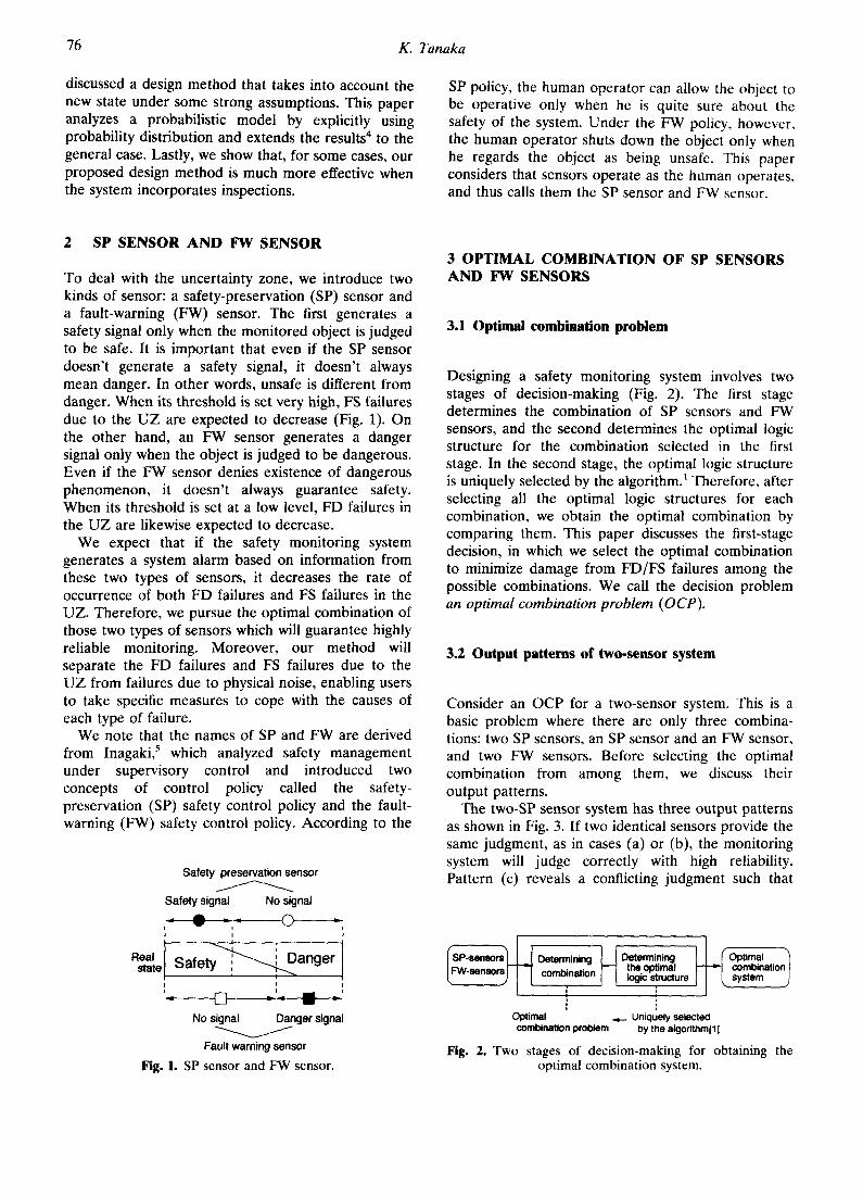
To deal with the uncertainty zone, we introduce two kinds of sensor: a safety-preservation (SP) sensor and a fault-warning (FW) sensor. The first generates a safety signal only when the monitored object is judged to be safe. It is important that even if the SP sensor doesn't generate a safety signal, it doesn't always mean danger. In other words, unsafe is different from danger. When its threshold is set very high, FS failures due to the UZ are expected to decrease (Fig. 1). On the other hand, an FW sensor generates a danger signal only when the object is judged to be dangerous. Even if the FW sensor denies existence of dangerous phenomenon, it doesn't always guarantee safety. When its threshold is set at a low level, FD failures in the UZ are likewise expected to decrease.

We expect that if the safety monitoring system generates a system alarm based on information from these two types of sensors, it decreases the rate of occurrence of both FD failures and FS failures in the UZ. Therefore, we pursue the optimal combination of those two types of sensors which will guarantee highly reliable monitoring. Moreover, our method will separate the FD failures and FS failures due to the UZ from failures due to physical noise, enabling users to take specific measures to cope with the causes of each type of failure.

We note that the names of SP and FW are derived from Inagaki, 5 which analyzed safety management under supervisory control and introduced two concepts of control policy called the safety- preservation (SP) safety control policy and the fault- warning (FW) safety control policy. According to the

Safety preservation sensor Safety signal No signal

I i

Real state ' t y ~ ' S a f e ' ' , a n g e r

I i i I

No signal Danger signal

Fault warning sensor

Fig. 1. SP sensor and FW sensor.

3 OPTIMAL COMBINATION OF SP SENSORS AND FW SENSORS

3.1 Optimal combination problem

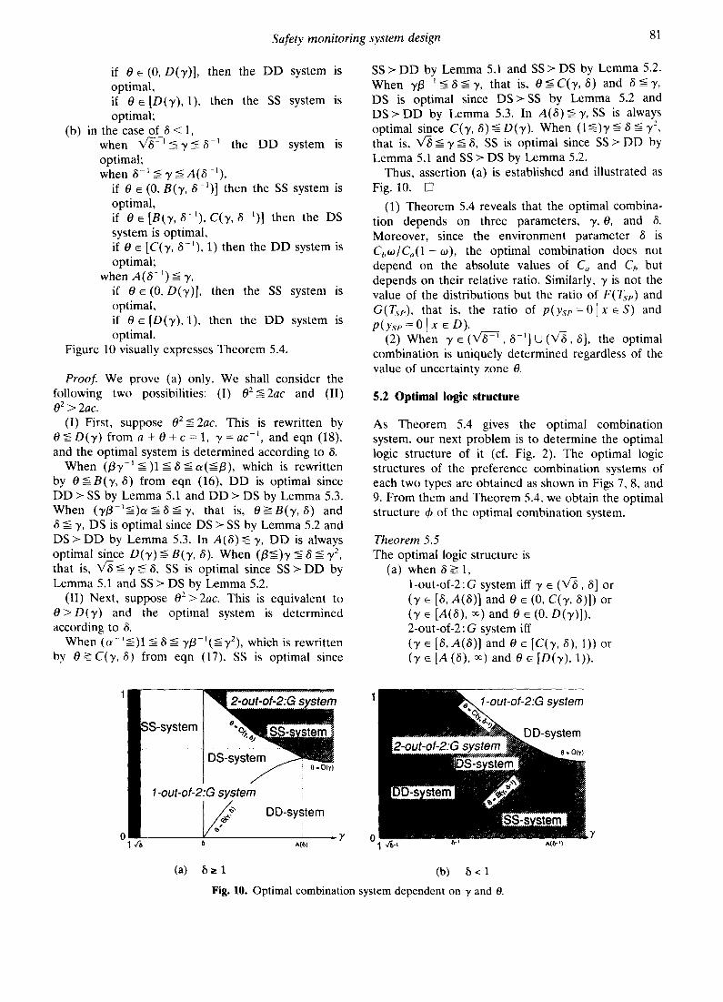
Designing a safety monitoring system involves two stages of decision-making (Fig. 2). The first stage determines the combination of SP sensors and FW sensors, and the second determines the optimal logic structure for the combination selected in the first stage. In the second stage, the optimal logic structure is uniquely selected by the algorithm, t Therefore, after selecting all the optimal logic structures for each combination, we obtain the optimal combination by comparing them. This paper discusses the first-stage decision, in which we select the optimal combination to minimize damage from FD/FS failures among the possible combinations. We call the decision problem an optimal combination problem (OCP).

3.2 Output patterns of two-sensor system

Consider an OCP for a two-sensor system. This is a basic problem where there are only three combina- tions: two SP sensors, an SP sensor and an FW sensor, and two FW sensors. Before selecting the optimal combination from among them, we discuss their output patterns.

The two-SP sensor system has three output patterns as shown in Fig. 3. If two identical sensors provide the same judgment, as in cases (a) or (b), the monitoring system will judge correctly with high reliability. Pattern (c) reveals a conflicting judgment such that

~ Determining H Determining I1 ~'Optimal the optimal ~ combination

combination logic structure • I} ~ system

Optimal ..,__ Uniquely selected combination problem by the algorithm[I]

Fig. 2. Two stages of decision-making for obtaining the optimal combination system.

Safety monitoring system design 77

(a)

(b)

Safety signal No signal

. . . . . . . . . . t

. . . . . I

. . . . I

I c ) . . . . . . . . . . t _ _ 1 ~ v I

Fig. 3. Three output patterns of two SP sensors.

added information. In Section 7, we analyze conditions under which detailed inspection is effective. In pattern (d), it seems impossible to judge whether the object is safe or dangerous. Rather, (d) suggests that either or both of the sensors have failed from physical trouble and that both sensors should be inspected. In other words, this pattern includes information about physical failures in sensors. Thus, (c) and (d) provide different quality information from safety or danger of the object.

Beginning in the next section, we show a probabilistic approach to the optimal combination problem without inspection.

one sensor affirms the safety of the object but the other denies the safety. If the sensor system generates an alarm for this output, the logic structure of the system is 1-out-of-2 type. If not, it is 2-out-of-2 type. The optimal logic structure is decided to be either of them by the algorithm, ~ which depends on such parameters as conditional probabilities of FD/FS failures, loss values and so on. The output patterns of the two-FW sensor system are similar.

A system with an SP sensor and an FW sensor has four output patterns as shown in Fig. 4. Pattern (a) reveals that the SP sensor affirms the safety of the object and the FW sensor denies the existence of a dangerous phenomenon. This output is a standard pattern for the safe object. Pattern (b) is a similar but inverse case. Pattern (c) reveals that the SP sensor denies the safety of the object but the FW sensor denies the existence of a dangerous phenomenon. This means that the state is in the UZ, and it is difficult to judge correctly whether the object is safe or dangerous. In this case, there are two methods to judge. One is to judge based on some rule decided in advance, which makes it possible to monitor the state automatically without adding other information. The other is to inspect the state in detail and to judge from

(a)

(b)

(c)

(d)

Fig. 4. Four

Safety signal s e . . . . . . . . . . . I

F W I = . . . . ='- , . . . . . . I

- - !

Danger signal output patterns of an SP sensor and

s e n s o r .

an FW

4 DESCRIPTION OF PROBABILISTIC MODEL

4.1 Evaluation function

In this section, we describe the OCP using the probabilistic model. 1 The monitoring system must be optimized by minimizing the expected value of the sum of losses generated by FD failures and FS failures in the system. That is, the system must be designed to minimize the expected value of the sum of losses 1 = E[Z I alarm is generated for a safe object] + E[Z I no alarm is generated for a dangerous object] where Z is a random variable denoting the system damage.

Let X be a set of states of the monitored object in the real world and assume X to be exclusively partitioned into a domain of safety S and a domain of danger D, that is, X = S UD. Let x denote a state which reveals the actual state; x ~ S means that the object is safe and x E D means that the object is dangerous. Consider a safety monitoring system consisting of n identical sensors which monitor the same characteristic. Each sensor monitors a totally ordered value ~(x) for the real state x and, when the threshold is T, the sensor outputs 0 if rl(x) _-_- T, while it outputs 1 if ~7(x) > T.

Let us distinguish the output variable of the SP sensor and the FW sensor by YsP and yFw, respectively. It is important that the SP sensor and FW sensor are identical but have different thresholds; Tse and Trw. Therefore, the i-th SP sensor outputs yse(i) E {0, 1} where 0 means safe and 1 means unsafe, while the j-th FW sensor outputs Ym¢(]) ~ {0, 1} where 0 means not dangerous and 1 means dangerous. A sensor output vector of an n-sensor system is denoted y = (yse(1) . . . . . yse(k), y~w(k + 1) . . . . . y~w(n)) (see Fig. 5); and + denotes the logical structure function from a sensor state vector y to a system output in {0, 1} where 0 means no system alarm generation and 1 means a system alarm generation.

Next, we show the evaluation function. Denote by C, the loss caused by an FS failure of the system, and denote by Ch the loss due to an FD-failure. Let

78 K. Tanaka

" / - . . . . . . . . . . . . . . . . . . . . . . . /

Real states~( S se. o,

~ FW sensor ~ ~ * (y)

i ~ FWsens°rlY~(") I

Fig. 5. Safety monitoring system model.

oJ = p(x e D). Then, the expected loss I is expressed as follows:

I = K ~] (1 - ~b(y))p(y [ x e D) Y

+ L ~] &(y)p(y [ x e S), (1) Y

where K = Cb¢o and L = C,(1 - ¢o). The loss I can be rewritten as

I = K - ~ ~b(y)g(y), (2) Y

where

g(y) = K . p ( y Ix e D ) - L .p (y Ix e S). (3)

Then, the optimal structure function & is obtained by the following rule:

1 i f g ( y ) > 0 ~(Y)= 0 i fg(y)-<0. (4)

Our problem is to minimize I by controlling the combination of SP sensors and FW sensors, that is, controlling the values of p(y Ix • S) and p(y Ix e D) at the design level. If sensors are mutually independent, p (y Ix • S) k ' S) = I]i=~ p(ysp(l) IX • ×rI,%~+~p(yFw(i) [ x • S).

4.2 Distribution of SP sensor and FW sensor

We describe p ( y l x e S ) and p ( y l x e D ) by using distribution functions. All sensors have the same distribution because they are assumed to be identical. Let the conditional distribution of p(t Ix E S) for observed value t = ~(x) be F(t) and the conditional distribution of p(t Ix c D) be G(t). Since the SP sensor and the FW sensor have different thresholds, Tsp and TFW, P(YsP Ix) and P(YFw IX) are expressed as functions of the thresholds Tsp and TFW, respectively, as follows.

(a) SP sensor: P(YsP =0 Ix • S)

= p(no alarm I safety, SP sensor) = F(Tsp)

P(YsP =0 Ix e D) = p(no a larm[danger , SP sensor) = G(Tsp)

p(ysP = 1 b x s ) = p(alarm I safety, SP sensor) = 1 - F(Tse)

P(Yse = 1 Ix e D) = p(alarm [ danger, SP sensor) = 1 - G(Tsp)

(b) FW sensor: P(YFw =0 IX e S)

= p(no alarm I safety , FW sensor) = F(TFw)

P(Y~v = O [ x ~ D ) = p(no alarm I danger, FW sensor) = F(TFw)

P(YFw = 1 Ix ~ S) = p(alarm [ safety, FW sensor) = 1 - F(TFw)

P(YFw = 1 Ix e D) = p(alarm I danger, FW sensor) = 1 - G(Trw)

If there exists a density function f ( x ) of F(x), F(Tse) =p(r / (x) < Tse Ix e D) = fTsp f ( t ) dt, and 1 - F(Tsp) = frs,.f(t) dt.

In the next section, we determine the optimal combination of sensors in a system to minimize I, given distributions F and G, and two thresholds Tse and TFw.

5 ANALYTICAL APPROACH TO OPTIMAL COMBINATION PROBLEM

5.1 Optimal combination

We call a system consisting of n sensors with optimal logic structure an optimal structured system. Let (n;k~, k2)-system denote the optimal structured system consisting of kt SP sensors and k2 FW sensors ( n = k ~ + k 2 ) . Using these terms, we describe a procedure for solving the optimal combination problem OCP. The OCP aims to select the optimal combination system from n + 1 optimal structured systems {(n. k, n - k)-system I k = 0, 1 . . . . . n}. First, we compute the expected value of losses {l(k); k =0 , 1 . . . . . n}, where I(k) is the value for the optimal logic structures of (k, n - k)-system consisting of k SP sensors and n - k FW sensors. Then, we select the minimum l ( k ) value.

In order to analyze the OCP for a basic two-sensor system, we assume that:

(A1) sensors are mutually independent, (A2) 0 < 0 < 1, where F(TFw) - F(Tse) = O, (A3) F(Tsp) -> 1 - F(T~w). (A1) means that the output of each sensor is not

influenced by the outputs of any other sensor. (A2) reveals that TFW is strictly greater than Tse. The value 0 shows probability of the uncertainty zone (Fig. 6),

Safety monitoring system design 79

f(t)l

g(t)

Ts, TFW t

% T~w t

better type of combination in each pair of three system types.

Lemma 5.1 (a) When 02 =< 2F(Tse)(1 - F(Tcw)),

SS > DD if and only if (iff)

~ 2 ~ 6<=1 or/3 <=63" 2

D D > S S iff y - z< /5 <-/3-~ or 1 =<6_-</3.

(b) When 02 > 2F(Tsp)(1 - F(T~w)).

SS > DD iff 1 =< 6 <= 3'2,

D D > S S iff 3 '-~<6=<1.

Fig. 6. Distribution functions of sensor.

and if 0 = 0, an SP sensor would be not distinguish- able from an FW sensor. (A3) is a natural assumption and if sensor doesn't satisfy (A3), we shouldn't call it an SP sensor any longer.

Moreover, to avoid needless complexity in our model, we assume that

~" G(Tse) = 1 - F(TFw) (A4) /

(F(Tsp) = 1 G(Tvw).

This assumption establishes the two distributions F and G as symmetric for the two thresholds. G(TFw)-G(Ts .p )=O also follows from (A2) and (A4).

Now we denote the three types of sensor system as SS, DD, and DS, where S means an SP sensor and D means an FW sensor. When one system, say SS, is preferable to another, say DD, we denote this by SS > DD. This means that Iss is equal to or less than IDD where ISS(IDD ) is the expected loss of the SS (DD) system (cf. eqn (1)). Also, we set

K C~,oo 6= L C, , (1- to)' (5)

F(T~v) ( F(TFw)] (6)

l ---K--~se) \ = G(TFw)]'

F(Tsp) + F(TFw)

2 - F(Tse) - F(TFw)

F(Tsp) + F(TFw) ], v

F(rse) ( F(Tsp)) (8)

3"-1 - F(r ) t GSF-sfisS

Here, 6 is an uncontrollable environment constant. The next lemmas give the criteria for selecting the

Proof. Let gs(Y) and gD(Y) denote g(y) in eqn (3) for SS and DD, respectively. Let a and c be probabilities defined by a = F(Tsp) and c = G(Tse). Then, we have a + 0 + c = 1 from (A2) and (A4) (cf. Fig. 6). Now, gs(Y) is calculated by (A1) as follows.

gs(00) : Kp(OO l x E O ) - Lp(OO I x ~ S)

= Kc 2 - La 2 (9)

gs(01) = gs(10) = K(a + O)c - La(O + c)

gs( l l ) = K(a + 0 ) : - L(O + c) 2

From the eqns (9), we have gs(O0)>O iff 6 > 3,2; gs (01)>0 iff 6>3,a-1; and g s ( l l ) > 0 iff 8 > a -2. It follows from 3'2 > 3'a-~ = a-2 that if gs(O0) > 0 then gs (01)>0 and that if gs (01)>0 then g s ( l l ) > 0 . Accordingly, when gs(O0)> 0, that is, 6 > 3'2, the SS system always generates a system alarm since g s ( y ) > 0 for all y. On the other hand, when gs(ll)<=0, that is 6<=a 2, SS never generates a system alarm since gs(Y)=<0 for all y. Hence, SS is useful only when a - 2 < 6 <-_3, 2. Similarly, the DD

-2 <~ ~ 0/2, system is useful only when 3' 15 < Therefore, we compare SS with DD in only 3' 2 < 15 =< 3'~.

We shall consider the following two possibilities: (a) 02 <= 2ac and (b) 02 > 2ac.

(a) Suppose 02<-2ac. Then we have 1=<3,a-1= < /3 N 3"2 under (A3).

(i) When 6 satisfies 3"a-~ </5 =< 3':, eqns (2) and (4) lead to the difference,

t , , o - t ~ -- { K - ( g o O 1 ) + 2go(m))}

- {K - (gs( l l ) + 2gs(01))}

= { K ( O + 2c) - L(ea + 0)}0 0 0 )

since go(01) > 0 and gs(01) > 0. Then, by 0 ~ 0

80 K. Tanaka

from (A2), SS > DD if and only if (iff) {5 >/3. Therefore, SS > DD iff 8 ~ [/3, .y2], and DD > SS iff {5 e ( 3 , a - ' , / 3 ] . (ii) When a y -t < {5 N Y{i-t, the difference is

1DD -- ISS = gs ( l l ) - (go( l l ) + go(01))

= (K - L)(02 - 2ac) (1l)

from gD(01) > 0 and gs(01) -<- 0. Therefore, under 02<=2ac, S S > D D i f f 6 e ( a y -t , 1 ] a n d D D > S S iff 8 e [1, "y{l-l]. (iii) When y -2 < 8 =< a y -~, the difference is

1DO - Iss = gs( l l ) - go(11)

= {K(O + 2a) - L(O + 2c)}0 (12)

from gD(01) =<0 and gs(01) ---< 0. Then, it follows from 0 # 0 that SS > DD iff {5 _->/3-1. Therefore, S S > D D iff 6 e [ / 3 - ~ , a y 1], and D D > S S iff 8 e (~,-2,/3-t] .

Thus, (i), (i i) and (ii i) imply that part (a) in Lemma 5.1.

(b) Now suppose 02> 2ac, then we have I-<_/3-<_ y a - t <_ yz under (A3).

When 7{i-~ < {5 -< 3, 2, SS > DD always holds since /3 < 7a-1 and eqn (10). When {i,y--I < 8 ~ 'y{i I, it follows from eqn (11) that S S > D D iff {5 • [1, ya -~] a n d D D > S S i f f S e ( a 7 1,1]. When 7-2<{5_-<{iy -I, DD > SS always holds since a y ~ </3 ~ and eqn (12).

These imply the part (b) in Lemma 5.1. []

Figure 7 illustrates Lemma 5.1. We note that the process of the proof provides the optimal logic structures. For example, if g ( 0 1 ) > 0 then it is 1-out-of-2:G system, while if g ( 0 1 ) < 0 then it is 2-out-of-2:G system. They are also included in the figure.

Lemma 5.2 (see Fig. 8) S S > D S iff {i-l~---8~'y/3-1 or y_-<6-<y 2,

D S > S S iff ({iy)-~<-_6<={i -l or y/3-1<--{5<=y.

The proof is omitted since it is similar to the proof of Lemma 5.1.

DO I/z) SS DO 'iz SS I , ~a (a) -z -t (aYt9 1 (ya-') p y

SS ( b ) - z z / z ' 1 / z 2/2 1/z

(a'F9 1 (ya-O y

F i g . 7 . Preference order between SS and DD dependent on 3. ((a), (b) in Lemma 5.1 k/2:k-out-of-2:G system).

- yp -~ y Y

Fig. 8. Preference order between SS and DS dependent on 3. (Lemma 5.2).

t, 'i',,, os:,i,, DD 7 os - I a ay

Fig. 9. Preference order between DD and DS dependent on 6. (Lemma 5.3).

system because 8 is an uncontrollable environment • constant but a, /3, y, and 0 are controllable

parameters. Moreover, we can rewrite {i and /3 as y and 0.

3 , + 0 {i = (13)

l + y O

27 - 0(7 - 1) /3 = (14)

2 + 0(~, - 1)

Therefore, Theorem 5.4 focuses on Y and 0 and gives the solution for the OCP without using a and/3. We set

A ( a ) = a 2 - (a - 1) (1 - ,,/1 + a2), (15 )

8 - y B(y, 8) - - - (16)

1 - yS '

C(y, 8 ) - 2 y ( 8 - 1) (17) ( 7 - 1)(7 + 8 ) '

v ~

D ( 7 ) - VT + y v ~ + V~" 08)

Lemma 5.3. (see Fig. 9) D S > D D iff 3,-~<-_6<-_/37 -~ or a<-{5<-87,

D D > D S iff y-z<{5<<_y-i or f ly -~<-8<-a.

The proof is omitted. As is shown in the proof of Lemma 5.1, these sensor systems are meaningful only when , / - z < 8 <_-7'. We note again that if 3,-2_ -> 8, no systems generate a system alarm and that if 3, 2 < {5, all the systems always generate a system alarm.

From these lemmas we obtain Theorem 5.4 which gives criteria for selecting the optimal combination. The expressions of the above lemmas are simple but not easy to use in designing a safety monitoring

Theorem 5.4 The OCP for a two-sensor system is solved as

follows: (a) in the case of 8 >_ 1,

when V~-< y =< {5, the SS system is optimal; when {5 _-< y <-_A({5),

if 0 E (0, B(y, {5)] then the DD system is optimal, if 0 E [B(,/, {5), C(y,{5)] then the DS system is optimal, if 0 E [C(y, {5), 1] then the SS system is optimal;

when A({5) <= y,

Safety monitoring system design 81

if 0 E (0, D(3')], then the D D system is optimal, if 0 e [D(7), 1), then the SS system is optimal;

(b) in the case of 6 < 1, when 6X/6-cx <- 3' _-__ 6 -~ the D D system is optimal; when 3 -~ <- 3' <-A(3-~),

if 0 ~ (0, B(3', 6-~)] then the SS system is optimal, if 0 e [B(3', 6-~), C(3', 6-~)] then the DS system is optimal, if 0 ~ [C(% 6-~), 1) then the D D system is optimal;

when A(3- ~) =< 3', if 0 e (0, D(y)] , then the SS system is optimal, if 0 e [D(3'), 1), then the D D system is optimal.

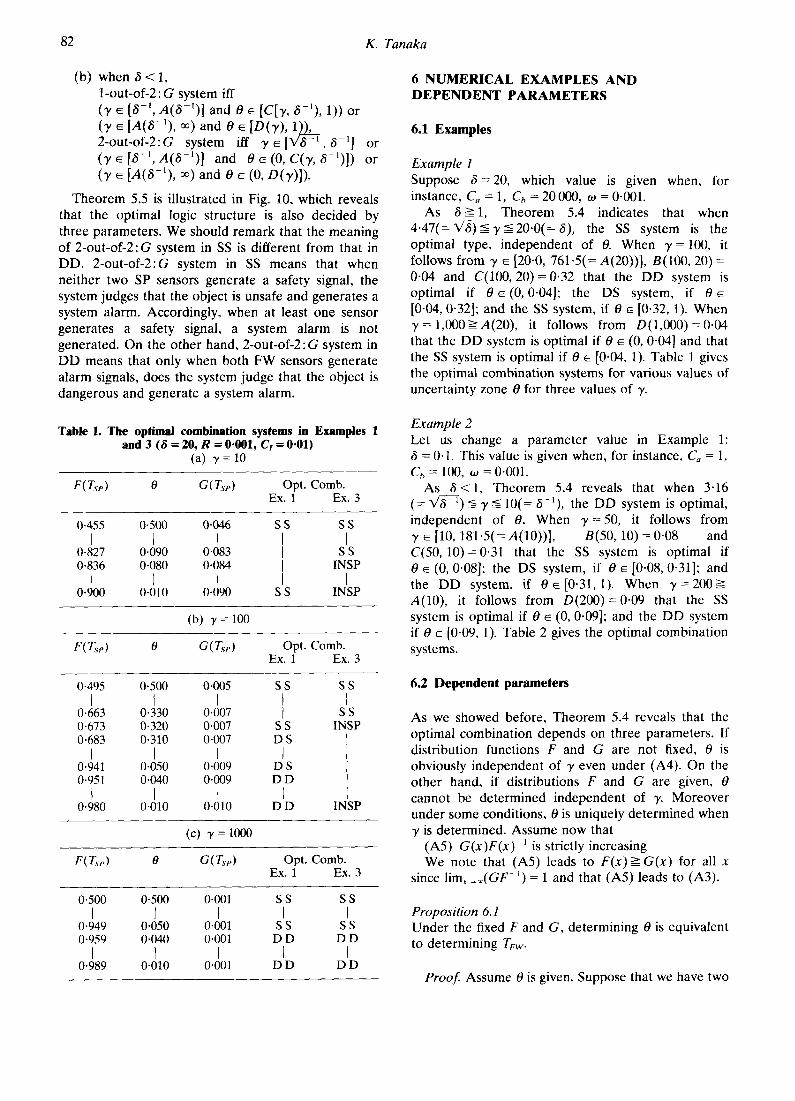
Figure 10 visually expresses Theorem 5.4.

Proof. We prove (a) only. We shall consider the following two possibilities: (I) 02~2ac and (II) 02 > 2ac.

(I) First, suppose 02<=2ac. This is rewritten by O<=D(3") f r o m a + 0 + c = l , 3 ' = a c z, a n d e q n (18), and the optimal system is determined according to 3.

When (/37 ~ <-)1 <= 3 <- a(-</3), which is rewritten by O<-B(3", 3) from eqn (16), D D is optimal since D D > SS by Lemma 5.1 and D D > DS by Lemma 5.3. When (7 /3-~<-)a~8-<3 ' , that is, 0>-B(7,3) and 6 <_- 3', DS is optimal since DS > SS by Lemma 5.2 and DS > D D by Lemma 5.3. In A(8)<- % D D is always optimal since D(3") <= B(3", 3). When (/3<-)3' <- 3 -< 3'2 that is, V~ <- 3' <-3, SS is optimal since SS > D D by Lemma 5.1 and SS > DS by Lemma 5.2.

(II) Next, suppose 02>2ac . This is equivalent to O>D(3") and the optimal system is determined according to 3.

When (a ~---)1 -<_ 3 <= 3'/3 1(~3'2), which is rewritten by 0 ~ C ( 3 ' , 8) from eqn (17), SS is optimal since

SS > D D by Lemma 5.1 and SS > DS by Lemma 5.2. When y/3-~<_-6-<7, that is, O<=C(y, 3) and 3-<_7, DS is optimal since D S > S S by Lemma 5.2 and DS > D D by Lemma 5,3. In A(6)<- 3', SS is always optimal since C(y, 3) <- D(7). When (1<=)7 <= 6 <- y 2, that is, V~ <- 3' <= 3, SS is optimal since SS > DD by Lemma 5.1 and SS > DS by Lemma 5.2.

Thus, assertion (a) is established and illustrated as Fig. 10. []

(1) Theorem 5.4 reveals that the optimal combina- tion depends on three parameters, 7, 0, and 8. Moreover, since the environment parameter 3 is Cboo/Co(1-w), the optimal combination does not depend on the absolute values of C,, and Ch but depends on their relative ratio. Similarly, 3' is not the value of the distributions but the ratio of F(Tsp) and G(Tsp), that is, the ratio of p(ysp=Olx ~ S) and P(YsP = 0 Ix e D).

(2) When 3' E ( 6X/ff --T , 3 -~] U (X/8,6], the optimal combination is uniquely determined regardless of the value of uncertainty zone 0.

5.2 Optimal logic structure

As Theorem 5.4 gives the optimal combination system, our next problem is to determine the optimal logic structure of it (cf. Fig. 2). The optimal logic structures of the preference combination systems of each two types are obtained as shown in Figs 7, 8, and 9. From them and Theorem 5.4, we obtain the optimal structure ~b of the optimal combination system.

Theorem 5.5 The optimal logic structure is

(a) when 6 >= 1, 1-out-of-2:G system iff 7 e (X/g, 6] or (3' e [6, a (6 ) ] and 0 e (0, C(3,, 3)]) or (7 e [A(6), ~) and 0 e (0, D(3')]), 2-out-of-2 : G system iff (3' ~ [6, A(6)] and 0 e [C(3', 6), 1)) or (3' e [a (3), ~) and 0 e [D(7), 1)),

0 B

2-out-of-2:G system

DS-system e - D(y)

1-out-of-2:G system

DD-system

A(6) 7 0

A(b-q

(a) 5 > 1 (b) 8 < 1

Fig. 10. Optimal combination system dependent on 3' and 0.

7

82 K. Tanaka

(b) when 8 < 1, 1-out-of-2: G system iff (3' • [6 -~, A(6-~)] and 0 • [C[3', 6-1), 1)) or (y • [A(3-~), oo) and 0 • [D(3'), 1~__, 2-out-of-2:G system iff 3 ' • [ V 6 - ' , 6 -~] or (3' • [~-1, A(6-~)] and 0 • (0, C(3', ~-1)]) or (3' • [A(6-t) , oo) and 0 • (0, D(3')]).

Theorem 5.5 is illustrated in Fig. 10, which reveals that the optimal logic structure is also decided by three parameters. We should remark that the meaning of 2-out-of-2:G system in SS is different from that in DD. 2-out-of-2:G system in SS means that when neither two SP sensors generate a safety signal, the system judges that the object is unsafe and generates a system alarm. Accordingly, when at least one sensor generates a safety signal, a system alarm is not generated. On the other hand, 2-out-of-2:G system in DD means that only when both FW sensors generate alarm signals, does the system judge that the object is dangerous and generate a system alarm.

Table 1. The optimal combination systems in Examples 1 and 3 (8 = 20, R = 0.001, Ct = 0.01)

(a) 3' = 10

F(Tsp) 0 G(Tsp) Opt. Comb. Ex. 1 Ex. 3

0.455 0.500 0.046 S S S S I I I I I

0.827 0-090 0"083 I S S 0.836 0-080 0.084 [ 1NSP

I I I I I 0.900 0.010 0.090 S S INSP

(b) y = lO0

F(Tse) 0 G(Tse) Opt. Comb. Ex. 1 Ex. 3

0.495 0.500 0-005 S S S S I I I t I

0"663 0.330 0.007 I S S 0.673 0-320 0-007 S S INSP 0-683 0.310 0-007 D S I

I I I I I 0.941 0-050 0-009 D S I 0"951 0-040 0.009 D D [

I L I I I 0"980 0"010 0.010 D D INSP

(c) 3, = 1000

F(Ts.) 0 G(Tse) Opt. Comb. Ex. 1 Ex. 3

0.500 0-500 0-001 S S S S I I I I I

0-949 0"050 0"001 S S S S 0-959 0"040 0.001 D D D D

I I I I I 0.989 0.010 0.001 D D D D

6 N U M E R I C A L E X A M P L E S A N D D E P E N D E N T P A R A M E T E R S

6.1 Examples

Example 1 Suppose 6 =20, which value is given when, for instance, 6", = 1, C~ = 20 000, to = 0.001.

As 6_->1, Theorem 5.4 indicates that when 4"47(= V6) =< 3' = 20.0(= 6), the SS system is the optimal type, independent of 0. When 3' = 100, it follows from 3' • [20.0, 761-5(= A(20))], B(100, 20) = 0-04 and C(100, 2 0 )=0 .3 2 that the DD system is optimal if 0 e ( 0 , 0 - 0 4 ] ; the DS system, if 0 e [0-04, 0.32]; and the SS system, if 0 • [0.32, 1). When 3' = 1,000 -> A(20), it follows from D(1,000) = 0.04 that the DD system is optimal if 0 • (0, 0.04] and that the SS system is optimal if 0 • [0-04, 1). Table 1 gives the optimal combination systems for various values of uncertainty zone 0 for three values of 3'.

Example 2 Let us change a parameter value in Example 1: 6 = 0.1. This value is given when, for instance. C, = 1, Cb = 100, w = 0-001.

As 6 < 1, Theorem 5.4 reveals that when 3-16 (= V6 -1) =< 3' =< 10(= 6-1), the DD system is optimal, independent of 0. When y = 5 0 , it follows from 3' E [10, 181.5(--A(10))], B(50, 10)= 0.08 and C(50, 10)=0.31 that the SS system is optimal if 0 e (0, 0.08]; the DS system, if 0 e [0.08, 0.31]; and the DD system, if 0 • [0.31, 1). When 3'=200>_- A(10), it follows from D (2 0 0 )=0 .0 9 that the SS system is optimal if 0 e (0, 0.09]; and the DD system if 0 e [0.09, 1). Table 2 gives the optimal combination systems.

6.2 Dependent parameters

As we showed before, Theorem 5.4 reveals that the optimal combination depends on three parameters. If distribution functions F and G are not fixed, 0 is obviously independent of 3' even under (A4). On the other hand, if distributions F and G are given, 0 cannot be determined independent of 3'. Moreover under some conditions, 0 is uniquely determined when 3' is determined. Assume now that

(A5) G(x)F(x)-1 is strictly increasing We note that (A5) leads to F(x)>= G(x) for all x

since lim . . . . (GF-') = 1 and that (A5) leads to (A3).

Proposition 6.1 Under the fixed F and G, determining 0 is equivalent to determining T~v.

Proof. Assume 0 is given. Suppose that we have two

Safety monitoring system design 83

Table 2. The optimal combination systems in Examples 2 and 3 (~ = 0"10, R = 0-001, Ci = 0.01)

(a) y = 5

F(Tse) 0 G (Ts~,) Opt. Comb. Ex. 1 Ex. 3

0.417 0'500 0-083 D D D D I I I I I

0-717 0"140 0"143 ] D D 0.725 0-130 0.145 [ INSP

I I I I [ 0-825 0-010 0" 165 D D INSP

(b) ~, = 50

F(Tse) 0 G(Ts,,) Opt. Comb. Ex. 1 Ex. 3

0.490 0.500 0-010 D D D D I I I I I

0.667 0.330 0"013 ] D D 0.677 0-320 0.014 D D INSP 0.686 (/.310 0.014 D S [

I I I I I 0-892 0"090 0"018 D S ] 0-902 0"080 0"018 S S I

I I I I I 0.970 0"010 0.019 S S INSP

(c) y = 200

F(Tse) 0 G(Tsp) Opt. Comb. Ex. 2 Ex. 3

0-498 0.500 0-003 D D D D I I I I I

0.896 0' 100 0"005 D D D D 0-906 0"090 0"005 S S S S

I I I I I 0-985 0.010 0-005 S S S S

7 EFFECT OF INSPECTION

We have so far discussed the optimal combination of sensors without inspection. As mentioned earlier, in the DS system, when neither the SP nor the FW sensor generates a signal, the object is considered in the uncertainty zone. This section discusses, in that case, whether it is effective to inspect the state in detail and to judge from additional information.

Let Ct denote inspection cost and R denote the probability that either the inspection cannot detect any actual danger, or damage will occur before inspection is complete. When inspection is preferred, the inspection cost C~ is incurred even if the object is safe. Also, if the object is dangerous, the expected value of the damage from incomplete inspection RCb is added to the inspection cost C~. If inspection is always complete, R should be set to zero. When we denote by ItusP the expected loss for the DS system with inspection activities and by lt)~ the expected loss without inspection, lmsp is obtained by revising eqn (2):

I, Nsp=K - ~ &(Y)g(Y) y ~ ( O l )

+ ( C , - (1 - R)Ch)wP(y : (01) Ix = 1)

+ c , ( 1 - , , , ) P ( y = ( O l ) ] x =-=- o )

J 'IDs + {(K - L) + (C, - (1 - R)K)}

× E(Tse)(1 - F(T~w)) if 6 ->_ l

: l I D s ~- ( C I - ( 1 - R)K)F(Tsp)

l × (1 - F ( T , w ) ) i f 6 < l

(19)

pairs of thresholds for the FW sensor and the SP sensor, (TFw, Tse) and (T~v, T~e) such that TFW -< T~w and F(TFw) - F(Tse) = F(T~w) - F(T~p) = 0. Then, F ( T F w ) - F(T~w) = F ( T s e ) - F(T~p) = G(T~-w) - G(TFw) from (A4). Accordingly, F(T~w)=F(T~w) and G(T~w) = G(TFw) since F and G are increasing functions. If Trw~T'~w, then G(Trw)F(TF~) - t= G(T~v)F(T~w) -j contradicts (A5). Therefore , TFw = T;w.

On the other hand, if TFW is given, Tsp is also uniquely decided from (A4) and (A5). []

Corollary 6.2 Under the fixed F and G, determining 0 is equivalent to determining 3'-

This corollary is derived by Proposition 6.1 and (A5). This reveals consequently that the optimal combination determination depends only on the uncertainty zone 0 and the environment parameter 6.

From eqn (19), when a > 1, IINsP < IDS if and only if C~ < L - RK, and when 6 < 1, ]INSP < [DS if and only if C ~ < ( 1 - R ) K . These results lead to the next proposition.

Proposition 7.1 In the DS system, inspection is effective if and only if Ct < rain(K, L) - RK.

Example 3 Consider Examples 1 and 2 again. Suppose R = 0.001 and C~ -- 0.01. In Example 1 which is a case of 6 ->__ 1, L - R K - C t = 0 " 9 7 > 0 ; thus, the DS system with inspection is always better than that without it (see Table 1). On the other hand, in Example 2, a < 1 and ( 1 - R ) K - C t = 0 . 9 9 > O . Table 2 shows that the inspection is effective.

As the tables show, the DS system with inspection is preferable to the SS system (or DD system) which is the optimal combination without inspection in some c a s e s .

84 K. Tanaka

8 CONCLUSIONS which inspection increases the reliability of monitoring.

We have shown that the uncertainty zone can be effectively monitored when we use a design method utilizing a combination of SP sensors and FW sensors under certain conditions. Moreover, we indicated that the combination design method gives information about sensor failures to users. Our analytical results showed that the optimal combination for a two-sensor system and the optimal logic structure are determined by only three parameters, an environment parameter , the uncertainty zone and the ratio of the correct response probability to the wrong response one. The results indicate that the reliable monitoring system design depends on setting two thresholds Tsr and TFW, and their visual expression makes sensitive analysis possible. Lastly, we showed the conditions under

REFERENCES

1. Henley, E. J. & Kumamoto, H., Designing for Reliability and Safety Control. Prentice-Hall, New Jersey, 1985.

2. Phillips, M. J., k-out-of-n:G systems are preferable. IEEE Trans. Reliab., R-29 (1980) 166-'169.

3. Inoue, K., Kouda, T., Kumamoto, H. & Takami, I., Optimal structure of sensor systems with two failure modes. IEEE Trans. Reliab., 11-31 (1982) 119-120.

4. Tanaka, K., Reliable safety monitoring system by optimal combination of safety monitoring and danger monitoring. JSICE, 28 (1992) 726-732 (in Japanese).

5. Inagaki, T. & Inoue, K., Adaptive choice of a safety management scheme upon an alarm under supervisory control of a large-complex system. Reliab. Engng & System Safety, 39 (1993) 81-87.