Embed Size (px)
Citation preview
The Pennsylvania State University
The Graduate School
Department of Mechanical and Nuclear Engineering
RELIABLE CONTROL AND ONLINE MONITORING DESIGN FOR NUCLEAR POWER PLANT WITH IRIS DEMONSTRATION
A Thesis in
Nuclear Engineering
by
Yin Guo
2010 Yin Guo
Submitted in Partial Fulfillment of the Requirements
for the Degree of
Master of Science
May 2010

The thesis of Yin Guo was reviewed and approved* by the following:
Robert M. Edwards Professor of Nuclear Engineering Thesis Advisor Kostadin N. Ivanov Distinguished Professor of Nuclear Engineering
Jack S. Brenizer Jr. Professor of Mechanical & Nuclear Engineering Chair of Nuclear Engineering
*Signatures are on file in the Graduate School
iii
ABSTRACT
Development and deployment of small-scale nuclear power reactors and their
autonomous control and monitoring is part of the mission under the Global Nuclear Energy
Partnership (GNEP) program. The goals for this project are to investigate, develop, and validate
advanced methods for sensing, controlling, monitoring, and diagnosing the proposed small and
medium sized export reactors (SMR) and apply it to the International Reactor Innovative &
Secure (IRIS).
In this thesis, an online monitoring and reliable control system of nuclear power plants is
presented. First, a reliable LQG controller is obtained by solving ARE and LMI and by using
output feedback directly. The simulation results show that the LQG controller can maintain the
system stable when sensors drift in allowable range and perform well in tracking the reference
signal. Then, based on the dissipative port-controlled Hamiltonian theory, a nonlinear observer-
based feedback dissipation controller for the pressure control of the helical-coil steam generator
and a high gain online nonlinear state observer are designed. The asymptotical stability of both
the observer-based feedback dissipation controller and the high gain online nonlinear state
observer is guaranteed by the dissipation theory. The estimated states given by the state observer
converge to the real value, and the nonlinear state observer also guarantees the stability and
acceptable performance. The limitation of the reliable controller, the observer-based feedback
dissipation controller and the high gain online state observer are also discussed.
Recommendations for improvement and future research are discussed.
iv
TABLE OF CONTENTS
Chapter 1 Introduction ........................................................................................................ 1
1.1 Background and Motivation ................................................................................... 11.2 Thesis Organization ............................................................................................... 1
Chapter 2 Mathematical and Simulation Model for IRIS ..................................................... 3
2.1 Introduction to IRIS ............................................................................................... 32.1.1 IRIS Reactor ............................................................................................... 42.1.2 Helical-Coil Steam Generator ...................................................................... 6
2.2 Mathematical Model of IRIS Nuclear Power Plant ................................................. 72.2.1 Mathematical Model of Reactor ................................................................... 82.2.2 Mathematical Model of Helical-Coil Steam Generator ................................. 112.2.3 Mathematical Model of Steam Turbine ........................................................ 21
2.3 Simulation Model of IRIS Nuclear Power Plant ..................................................... 23
Chapter 3 Reliable LQG Controller Design with Sensor ...................................................... 24
3.1 Introduction to Reliable Control ............................................................................. 243.2 System Synthesis ................................................................................................... 26
3.2.1 Model Linearization .................................................................................... 263.2.2 Controller Design ........................................................................................ 27
3.3 Simulation ............................................................................................................ 303.4 Summary and discussion ........................................................................................ 32
Chapter 4 Nonlinear-Observed Feedback Dissipation Controller Design for HCSG Pressure Control .......................................................................................................... 34
4.1 Introduction ........................................................................................................... 344.2 Nonlinear State Space Model of HCSG .................................................................. 37
4.2.1 Subcooled Region ....................................................................................... 394.2.2 Boiling Region ............................................................................................ 405.2.3 Superheated Region .................................................................................... 414.2.4 Nonlinear State Space Model ...................................................................... 43
4.3 Observer-Based Feedback Dissipation .................................................................. 445.4 Simulation and Result ............................................................................................ 494.5 Summary ............................................................................................................... 54
Chapter 5 Online State Observer Design Based on Dissipation-Based High Gain Filter ....... 55
5.1 Introduction ........................................................................................................... 555.2 Methodology ......................................................................................................... 56
5.2.1 Problem Formulation ................................................................................... 565.2.1 Design and Robustness Analysis of DHGF .................................................. 58
5.3 Application in IRIS Nuclear Power Plant ............................................................... 62
v
5.3.1 State Space Model of IRIS Core for State-Observer Design ......................... 625.3.2 Numerical Simulation .................................................................................. 65
5.4 Conclusion ............................................................................................................ 73
Chapter 6 Conclusion and Suggestion ................................................................................. 75
6.1 Summary of Results ............................................................................................... 756.2 Future Work .......................................................................................................... 76
Reference ............................................................................................................................ 78
Appendix A Nomenclatures For OBFD Nonlinear State Space Model ......................... 84Appendix B Reliable LQG MATLAB Code ............................................................... 86
vi
LIST OF FIGURES
Figure 2-1. IRIS integral configuration ................................................................................ 6
Figure 2-2. IRIS steam generator module ............................................................................ 7
Figure 2-4. Schematic of the nodalization for a helical steam generator. .............................. 12
Figure 2-5.SIMULINK model of IRIS system. .................................................................... 23
Figure 3-1. Close loop system sketch. ................................................................................. 26
Figure 3-2.Dynamic response of case I. ............................................................................... 30
Figure 3-3.Control effects of case I. .................................................................................... 31
Figure 3-4.Dynamic response ofcase II. ............................................................................... 32
Figure 3-5. Control effects of case II. .................................................................................. 32
Figure 4-1. Lump model sketch of HCSG. ........................................................................... 38
Figure 4-2. Pressure response of HCSG: Case I ................................................................... 51
Figure 4-3. Length change of Lsc & Lb : Case I. ................................................................. 51
Figure 4-4. Feedwater flow rate : Case I .............................................................................. 52
Figure 4-5. Pressure response of HCSG: Case II .................................................................. 52
Figure 4-6. Length change of Lsc and Lb : Case II .............................................................. 53
Figure 4-7. Feedwater flow rate: Case II .............................................................................. 53
Figure 5-1. Transient response of nr in case I. ..................................................................... 67
Figure 5-2. Transient response of cr in case I. ...................................................................... 67
Figure 5-3. Transient response of Tf in case I. ..................................................................... 68
Figure 5-4. Transient response of Tcav in case I. ................................................................. 68
Figure 5-5. Transient response of nr in case II. .................................................................... 69
Figure 5-6. Transient response of cr in case II. .................................................................... 69
Figure 5-7. Transient response of Tf in case II. .................................................................... 70
Figure 5-8. Transient response of Tcav in case II. ................................................................ 70

vii
Figure 5-9. Transient response of nr in case III. ................................................................... 71
Figure 5-10. Transient response of Cr in case III. ................................................................ 72
Figure 5-11. Transient response of Tf in case III. ................................................................. 72
Figure 5-12. Transient response of Tcav in case III. ............................................................. 73

viii
LIST OF TABLES
Table 5-1. Inaccurate parameters of DHGF for Simulation of Case III. ................................ 71

ix
ACKNOWLEDGEMENTS
My research is supported by a U.S. Department of Energy NERI-C grant with
Pennsylvania State University and the University of Tennessee, under grant DE-FG07-
07ID14895.
I would like to thank Dr. Upadhyaya of University of Tennessee and Dr. Doster of North
Carolina State University for providing the Simulink models and Fortran Code of IRIS nuclear
power plant. I also would like to thank Mr. Xin Jin, another graduate student in our group, for
discussing problems with me. Dr. Edwards, thank you for providing me direction in my academic
career and guidance in completing this work.
Last but not least, I would like to express my sincerest gratitude to my family. Without
their support, I would not have been able to complete this study in The Pennsylvania State
University.

Chapter 1
Introduction
1.1 Background and Motivation
Development and deployment of small-scale nuclear power reactors and their
autonomous control and monitoring is part of the mission under the Global Nuclear Energy
Partnership (GNEP) program. The goals for this project are to investigate, develop, and validate
advanced methods for sensing, controlling, monitoring, and diagnosing the proposed small and
medium sized export reactors (SMR) and apply it to the International Reactor Innovative &
Secure (IRIS) [1]. IRIS is a smaller/medium power nuclear reactor designed by an international
consortium of companies, laboratories and universities which includes over 20 members from 10
countries [2]. Westinghouse Science and Technology Center is responsible in developing the
IRIS plant and in charge of the coordination of the international team. IRIS is in pre-application
licensing with the NRC and safety testing for Design Certification (DC) is expected to be
completed by 2010 with deployment in the 2015-2017 timeframe.
1.2 Thesis Organization
In this thesis, Chapter Two is an introduction to the IRIS nuclear power plant, including
the component description, the mathematical model and Simulink model. Chapter Three is a
description of the design steps taken that led to the reliable LQG control with sensor failure.
Chapter Four introduces the dissipation Hamiltonian theory. Then, based on this theory, an
observer-based output feedback dissipation controller is designed to stabilize the outlet pressure

2
of the Helical-Coil Steam Generator (HCSG). Furthermore, applying the dissipation Hamiltonian
theory again, a nonlinear high gain state observer is designed to estimate the state variables of the
reactor. Chapter Six provides a conclusion and ideas for future research.

Chapter 2
Mathematical and Simulation Model for IRIS
2.1 Introduction to IRIS
Details of the IRIS design and supporting analyses have been previously reported and the
reader is directed to the listed references [3][4][5]. The purpose of this chapter is to provide a
review of the IRIS characteristics. IRIS is a pressurized water reactor that utilizes an integral
reactor coolant system layout. The IRIS reactor vessel houses not only the nuclear fuel and
control rods, but also all the major reactor coolant system components including pumps, steam
generators, pressurizer, control rod drive mechanisms and neutron reflector. The IRIS integral
vessel is larger than a traditional PWR pressure vessel, but the size of the IRIS containment is a
fraction of the size of corresponding loop reactors, resulting in a significant reduction in the
overall size of the reactor plant. IRIS has been primarily focused on achieving design with
innovative safety characteristics. The first line of defense in IRIS is to eliminate event initiators
that could potentially lead to core damage. In IRIS, this concept is implemented through the
“safety-by design” approach, which can be simply described as “design the plant in such a way as
to eliminate accidents from occurring, rather than coping with their consequences.” If it is not
possible to eliminate certain accidents altogether, then the design inherently reduces their
consequences and/or decreases their probability of occurring. The key difference in the IRIS
“safety-by-design” approach from previous practice is that the integral reactor design is
conducive to eliminating accidents, to a degree impossible in conventional loop-type reactors.
The elimination of the large LOCAs, since no large primary generations of the reactor vessel or
large loop piping exist, is only the most easily visible of the safety potential characteristics of

4
integral reactors. Many others are possible, but they must be carefully exploited through a design
process that is kept focused on selecting design characteristics that are most amenable to
eliminate accident initiating events.
2.1.1 IRIS Reactor
The IRIS core and fuel assemblies are similar to those of a loop type Westinghouse PWR
design. An IRIS fuel assembly consists of 264 fuel rods with a 0.374 in. o.d. in a 17×17 square
array. The central position is reserved for in-core instrumentation, and 24 positions have guide
thimbles for the control rod. Low-power density is achieved by employing a core configuration
consisting of 89 fuel assemblies with a 14-ft (4.267 m) active fuel height, and a nominal thermal
power of 1000 MWt. The resulting average linear power density is about 75% of the AP600
value. The improved thermal margin provides increased operational flexibility, while enabling
longer fuel cycles and increased overall plant capacity factors. Reactivity control is accomplished
through solid burnable absorbers, control rods, and the use of a limited amount of soluble boron
in the reactor coolant. The reduced use of soluble boron makes the moderator temperature
coefficient more negative, thus increasing inherent safety. The core is designed for a 3–3.5-year
cycle with half-core reload to optimize the overall fuel economics while maximizing the
discharge burnup. In addition, a 4-year straight burn fuel cycle can also be implemented to
improve the overall plant availability, but at the expense of a somewhat reduced discharge
burnup.
The IRIS reactor coolant pumps are of a “spool type”, which has been used in marine
applications, and are being designed and will soon be supplied for chemical plant applications
requiring high flow rates and low developed head. The motor and pump consist of two concentric
cylinders, where the outer ring is the stationary stator and the inner ring is the rotor that carries
5
high specific speed pump impellers. The spool type pump is located entirely within the reactor
vessel, with only small penetrations for the electrical power cables and for water cooling supply
and return. Further, significant qualification work has been completed on the use of high
temperature motor windings. This and continued work on the bearing materials has the potential
to eliminate even the need for cooling water and the associated piping penetrations through the
RV. This pump compares very favorably to the typical canned motor RCPs, which have the
pump/impeller extending through a large opening in the pressure boundary with the motor outside
the RV. Consequently, the canned pump motor casing becomes part of the pressure boundary and
is typically flanged and seal welded to the mating RV pressure boundary surface. All of this is
eliminated in IRIS. In addition to the above advantages derived from its integral location, the
spool pump geometric configuration maximizes the rotating inertia and these pumps have a high
run-out flow capability. Both these attributes mitigate the consequences of LOCAs (Loss of
Coolant Accidents). Because of their low developed head, spool pumps have never been
candidates for nuclear applications. However, the IRIS integral RV configuration and low
primary coolant pressure drop can accommodate these pumps and together with the assembly
design conditions can take full advantage of their unique characteristics. The structure of the IRIS
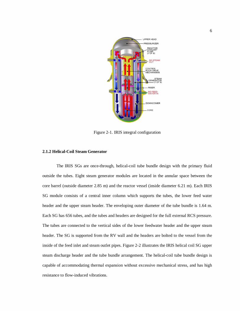
reactor is shown in Figure 2-1.
6
Figure 2-1. IRIS integral configuration
2.1.2 Helical-Coil Steam Generator
The IRIS SGs are once-through, helical-coil tube bundle design with the primary fluid
outside the tubes. Eight steam generator modules are located in the annular space between the
core barrel (outside diameter 2.85 m) and the reactor vessel (inside diameter 6.21 m). Each IRIS
SG module consists of a central inner column which supports the tubes, the lower feed water
header and the upper steam header. The enveloping outer diameter of the tube bundle is 1.64 m.
Each SG has 656 tubes, and the tubes and headers are designed for the full external RCS pressure.
The tubes are connected to the vertical sides of the lower feedwater header and the upper steam
header. The SG is supported from the RV wall and the headers are bolted to the vessel from the
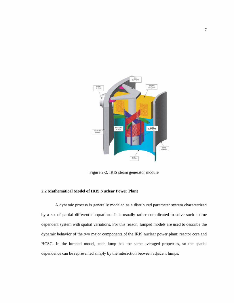
inside of the feed inlet and steam outlet pipes. Figure 2-2 illustrates the IRIS helical coil SG upper
steam discharge header and the tube bundle arrangement. The helical-coil tube bundle design is
capable of accommodating thermal expansion without excessive mechanical stress, and has high
resistance to flow-induced vibrations.
7
Figure 2-2. IRIS steam generator module
2.2 Mathematical Model of IRIS Nuclear Power Plant
A dynamic process is generally modeled as a distributed parameter system characterized
by a set of partial differential equations. It is usually rather complicated to solve such a time
dependent system with spatial variations. For this reason, lumped models are used to describe the
dynamic behavior of the two major components of the IRIS nuclear power plant: reactor core and
HCSG. In the lumped model, each lump has the same averaged properties, so the spatial
dependence can be represented simply by the interaction between adjacent lumps.
2.2.1 Mathematical Model of Reactor
1fT
2fT
fnT
cinT
coutT
1cavT
2cavT
cavnT
( 1)cout nT −
1coutT
2coutT
Fuel Rod Coolant
The nth cell
The 2nd cell
The 1st cell
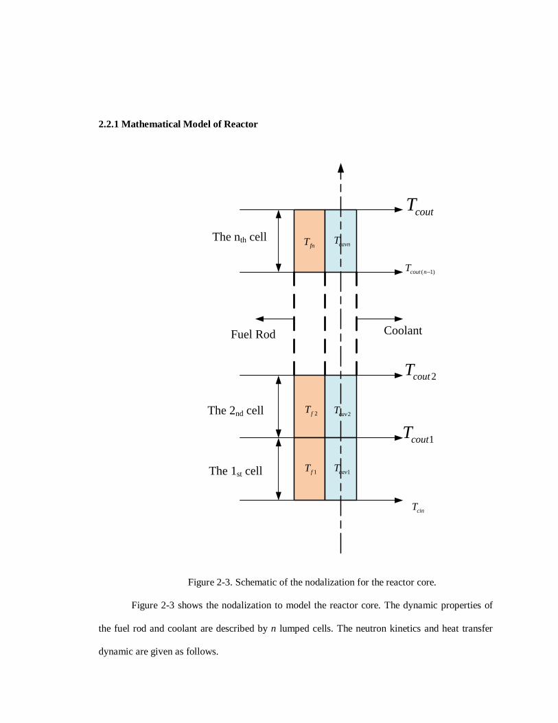
Figure 2-3. Schematic of the nodalization for the reactor core.
Figure 2-3 shows the nodalization to model the reactor core. The dynamic properties of
the fuel rod and coolant are described by n lumped cells. The neutron kinetics and heat transfer
dynamic are given as follows.
9
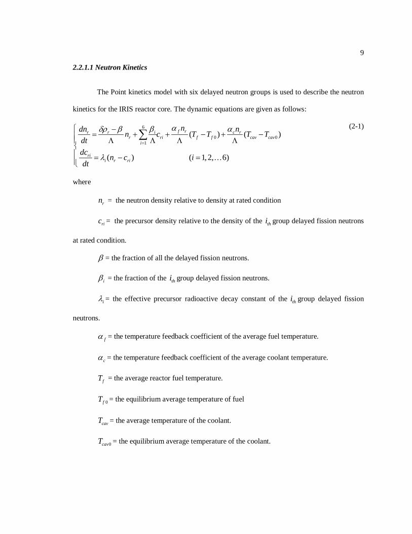
2.2.1.1 Neutron Kinetics
The Point kinetics model with six delayed neutron groups is used to describe the neutron
kinetics for the IRIS reactor core. The dynamic equations are given as follows:
6
0 01
( ) ( )
( ) ( 1, 2, 6)
f ri c rr rr ri f f cav cav
i
rii r ri
n ndn n c T T T Tdtdc n c idt
αβ αδρ β
λ
=
−= + + − + − Λ Λ Λ Λ
= − =
∑
(2-1)
where
rn = the neutron density relative to density at rated condition
ric = the precursor density relative to the density of the thi group delayed fission neutrons
at rated condition.
β = the fraction of all the delayed fission neutrons.
iβ = the fraction of the thi group delayed fission neutrons.
iλ = the effective precursor radioactive decay constant of the thi group delayed fission
neutrons.
fα = the temperature feedback coefficient of the average fuel temperature.
cα = the temperature feedback coefficient of the average coolant temperature.
fT = the average reactor fuel temperature.
0fT = the equilibrium average temperature of fuel
cavT = the average temperature of the coolant.
0cavT = the equilibrium average temperature of the coolant.

10
2.2.1.2 Heat Transfer in the Reactor Core
Some assumptions are given to provide a simple model of each lumped cell in Figure 2-3:
(1) the fuel element is homogeneous, so one-dimensional thermo-dynamic equations can be
achieved. (2) the thermal power is produced by the fission products and radiation process such as
beta-radiation and gamma-radiation, but here the heat produced by the radiation process is
neglected and (3) the temperature profiles of the fuel elements and the coolant inside the reactor
core are assumed to be smooth. Thus a lumped parameter model for the thi cell can be given as
follows:
_ 0_ _
__ _
2 2
f if i cav i r
f f f
cav icav i f i cin
c c c
dT PT T ndt
dT M MT T Tdt
µ µ µ
µ µ µ
Ω Ω= − + +
+ Ω Ω = − + +
(2-2)
where,
_f iT = the average fuel temperature of the thi cell.
_cav iT = the average coolant temperature of the thi cell.
Ω = the heat transfer coefficient between the fuel and coolant.
fµ =the total heat capacity of the fuel of the thi cell.
cµ = the total heat capacity of the coolant of the thi cell.
M = the value of the coolant flowrate times heat capacity of the coolant in the thi cell.
0P = the rated power distributed in the thi cell.

11
2.2.2 Mathematical Model of Helical-Coil Steam Generator
To build the lumped parameter model of HCSG, in addition to the assumptions implied in
a lumped model, the other major assumptions are as follows:
1) Only one pressure is used to characterize the superheated region.
2) The superheated vapor satisfies ideal gas law modified by an expansion coefficient.
3) The temperature of the second node in the subcooled region is equal to the saturated
temperature.
4) The pressure drop between superheated region and saturated region is constant during
any perturbation
5) The pressure drop between the saturated region and the subcooled region is constant
during any perturbation
6) The steam quality in the boiling region can be assumed as a linear function of the
axial coordinate so the density in the boiling region can be approximated as a function of steam
pressure.
7) The steam generation rate assumes to be equal to the boiling rate.
8) The heat transfer coefficient for the superheated region, the saturated region and the
subcooled region is assumed constant.
2.2.2.1 Nodalization
Figure 2-4 shows the nodalization to model the dynamic behavior of HCSG system.
Three regions, subcooled region, saturated region and superheated region, are used to characterize
the significant difference of heat transfer and hydraulic behavior. In each region, two lumps with
each volume are used to consider the axial temperature changes. Correspondingly, six metal
12
Tp1
Tp2
Tp3
Tp4
Tp5
Tp6
Tw1
Tw2
Tw3
Tw4
Tw5
Tw6
Ts1
Ts2
Tsat1
Tsat2
Tsc1
Tsc2 Feed water
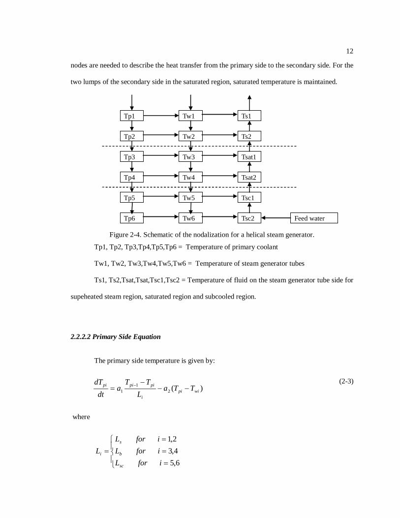
nodes are needed to describe the heat transfer from the primary side to the secondary side. For the
two lumps of the secondary side in the saturated region, saturated temperature is maintained.
Figure 2-4. Schematic of the nodalization for a helical steam generator.
Tp1, Tp2, Tp3,Tp4,Tp5,Tp6 = Temperature of primary coolant
Tw1, Tw2, Tw3,Tw4,Tw5,Tw6 = Temperature of steam generator tubes
Ts1, Ts2,Tsat,Tsat,Tsc1,Tsc2 = Temperature of fluid on the steam generator tube side for
supeheated steam region, saturated region and subcooled region.
2.2.2.2 Primary Side Equation
The primary side temperature is given by:
)(21
1 wipii
pipipi TTaL
TTa
dtdT
−−−
= − (2-3)
where
===
=6,54,32,1
iforLiforLiforL
L
sc
b
s
i

13
2/)(1ppxs
ppp
CAWC
aρ
=
2/)(2ppxs
wppw
CAPh
aρ
=
sL = superheated length.
bL = boiling length.
scL =subcooled length.
T =primary side temperature.
pW =coolant flow rate.
pC =specific heat.
ρ =density of the primary coolant.
xsA =flow area.
h =heat transfer coefficient.
wP =perimeter for heating.
In the above equations, subscript p and w refer to primary coolant and tube wall
respectively.
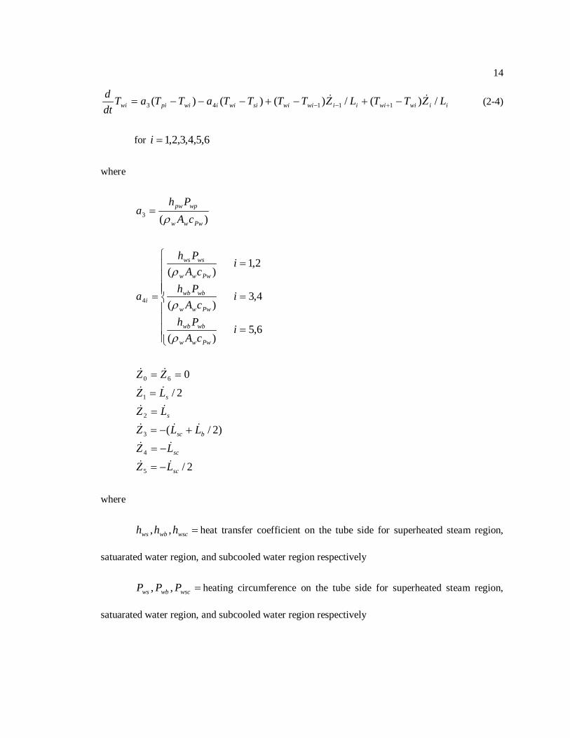
2.2.2.3 Metal Equations
The metal temperature is given by:
14
iiwiwiiiwiwisiwiiwipiwi LZTTLZTTTTaTTaTdtd /)(/)()()( 11143
−+−+−−−= +−− (2-4)
for 6,5,4,3,2,1=i
where
)(3Pwww
wppw
cAPh
aρ
=
=
=
=
=
6,5)(
4,3)(
2,1)(
4
icA
Ph
icA
Ph
icA
Ph
a
Pwww
wbwb
Pwww
wbwb
Pwww
wsws
i
ρ
ρ
ρ
2/
)2/(
2/
0
5
4
3
2
1
60
sc
sc
bsc
s
s
LZLZ
LLZLZLZZZ
−=
−=
+−=
=
=
==
where
=wscwbws hhh ,, heat transfer coefficient on the tube side for superheated steam region,
satuarated water region, and subcooled water region respectively
=wscwbws PPP ,, heating circumference on the tube side for superheated steam region,
satuarated water region, and subcooled water region respectively

15
2.2.2.4 Equations for the Superheated Region
The mass balance of the steam in the superheated steam nodes, node 1 and node 2, are
given by:
ss WWM −= 211 (2-5a)
212 WWM bs −= (2-5b)
where
sM = steam mass in the superheated region.
sW = steam flow rate to turbine, which is an external constraint imposed by the
controller.
bW = steam production rate.
The heat balance equations of the two superheated steam nodes, node 1 and node 2, are
given by:
1112211111 )( ssssssssss VPHWHWQVPHMdtd −−+=− (2-6a)
222212222 )( sssgbsssss VPHWHWQVPHMdtd −−+=− (2-6b)
where
sM = steam mass in the superheated region.
sP = steam pressure in the superheated region.
sV = steam volume in the superheated region.

16
sH =specific enthalpy of the steam.
21 , ss QQ = heat transfer rate to the two superheated nodes.
2/)( 111 swswswss TTLPhQ −=
2/)( 222 swswswss TTLPhQ −=
Assuming the pressure loss in the superheated steam region is small, we have:
21 sss PPP ==
Since specific enthalpy is a function of temperature and pressure, then we have:
ss
ss
s
ss P
PH
TTH
H ∂∂
+∂∂
= (2-7)
and
)( 1212 sss
sss TT
TH
HH −∂∂
=− (2-8)
Combining with the mass balance equations and the expansion of the specific enthalpy,
the energy balance equations can be rewritten as follows:
)()()( 2111112111 sspssssss
ssssspsspss TTCWQPV
PH
MMTTCTCM −−=−∂∂
+−+ (2-9)
)()( 222222 satspsbssss
ssspss TTCWQPV
PH
MTCM −−=−∂∂
+ (2-10)
The steam pressure in the superheated region can be described by compressibility
adjusted ideal gas law, which is given by :
17
)2/()( 21*
stmssssss MTTRMZVP += (2-11)
The time derivative of the steam pressure can then be determined by the following
equation:
sssssssssss
stm
ss LA
LAPTTMTTMM
RZP 1)()(2
2121
* −+++= (2-12)
where
stmM = mole mass of steam.
*sZ = steam expansion coefficient.
2.2.2.5 Equations for Boiling Region
The mass balance equation for the boiling region is given by:
bdbbsb WWLAdtd
−=)(ρ (2-13)
If we notice
dtdP
dPd
dtd sat
s
bb ρρ=
then
bdbsatbbsbbs WWPKLALA −=+ ρ
where
PK b
b ∂∂
=ρ
18
If we assume that the steam quality is a linear function of the axial position along the
channel, then
∫∫
∫+
==1
01
0
1
0)(
fgfb xvv
dx
dx
dxxρρ
In the operation pressure range, we have:
ssb PP 00552445.061594.1)( +=ρ
Therefore,
)/( bssatbbsbdbb APKLAWWL ρ −−=
fgbsatww
wbwbb hLTTT
UhW /)2
( 43 −+
=
dbW = flow rate leaving subcooled region to the saturated region.
fgh = vaporization heat.
2.2.2.6 Equations for Subcooled Region
In analogy to the boiling region, the mass balance equation for the subcooled region can
be given as follows:
scscscsscscscfwdb PKLALAWW −−= ρ
where
2/)( ffwscsc
scsc PP
K ρρρ
+∂
∂=
∂∂
=
fwW = feed water flow rate.
19
Heat balance equation for the subcooled region 1 is given by:
)()()(
121511
scdbscscpscscwscwscwscscscscp TWTWCTTLPhPV
dtTMCd
−+−=− (2-14)
Since the outlet temperature of the first subcooled node can be approximated by the
saturated temperature, then
)(2/)(2
][2
)(
25
1
satdbscscpscsatwscwscwsc
scscs
satscscsatscps
TWTWCTTLPh
PLA
PLKLTCA
−+−=
−+ ρ
where
PT
K sat
∂∂
=1
Heat balance equation for the subcooled region 2:
)(2/)(2
][2
)(
226
22
scscfwfwpscscwscwscwsc
scscs
scscscscscps
TWTWCTTLUh
PLA
TLLTCA
−+−=
−+ ρ
(2-15)
After simplification, we obtain
scscscscpsscscs
scscfwfwpscscwscwscwscsc
LLTCAPLA
TWTWCTTLPhT
/)(/(2*2
)()(*5.0
2
2262
−+
−+−=
ρ
If we assume 21 scsc MM = , then we have:
2/)( dbfwsc WWW +=
Substituting the expression of scW and dbW into the heat balance equation for the
subcooled region 1, we have:
)(5.0]1)2([2
)()(*5.0))()((5.0
1
12
252
satscscpsscsatscpscscscs
satscscfwpscsatwscwscwscsatscscps
sc
PLKCAPTTCKLA
TWTWCTTLPhTTCA
L
ρ
ρ
−−−−
−+−−
=
20
Noticing the pressure relationship between scP , satP and sP , we have
)(21
spsctpbsatsc PPPP ∆+∆+=
)(21
spsstpbsssat PPPP ∆+∆+=
where
scP =pressure at the subcooled region.
satP =pressure at the satuarated region.
tpbP∆ =two phase pressure loss in the boiling region.
spscP∆ =single phase pressure loss in the subcooled region.
spssP∆ =single phase pressure loss in the superheated region.
2.2.2.7 Equations for the Pressure Controller
The secondary side pressure is maintained by regulating the steam flow rate. The steam
flow rate satisfies the following equation:
s
sstss
WuCWW
τ−−
=)1(0 (2.16)
where
=u controller output.
=τ time constant.
0sW = initial steam flow rate on the secondary side.
stC = an adjustable parameter.
If a PI controller is used, the controller output has both the proportional part )(1 tu and the
integral part )(2 tu , which is given by:
21
)()(00
11 PP
PP
ktu settb −=
)()(
002
2
PP
PP
kdt
tdu settb −=
where
=1k the proportional gain.
=2k the integral gain.
tbP = the turbine header pressure.
setP = the turbine header pressure set-point.
0P = the nominal turbine header pressure.
2.2.3 Mathematical Model of Steam Turbine
Steam is the medium which connects steam generator and steam turbine. After generated
in the steam generators, passing through the steam line which connects the steam generators with
steam turbine, steam enters the cylinder of the steam turbine. The steam pressure and flow rate
into the steam turbine is adjusted by governing the high pressure control valve and high pressure
bypass valve. In the steam turbine, the internal energy of the steam converts into rotary kinetic
energy of the turbine rotor. Furthermore, the turbine rotor, as the prime mover, drives the rotor of
the generator, converts the rotary kinetic energy into electricity energy then electricity energy is
transported into the grid.
As mentioned above, the steam turbine is an important and complicated component of a
plant unit. For different research purpose, a specific mathematical model with different
complexity should be built. For example, if the steam expansion process, work process or
changes of steam state in a steam turbine is the focus of study, then a number of specific
22
properties of steam turbine should be taken into account, such as type of steam turbine, and etc.
Furthermore, the blade length and nozzle type determine how steam expands in a stage of the
turbine. Due to lack of steam turbine specification, and because the purpose of this research is to
study the responses of steam turbine in the various power conditions, a normalized and simplified
model is designed. The turbine is modeled as follows:
First calculate the pressure loss coefficient due to the throttling of control valve
2
(1 (1 ))
TCVauV
auV TCV TCV
KKT
T A b A
=
= − −
where K and b are constants which are determined by the property of the control valve. TCVK is
the pressure loss coefficient. TCVA is the valve position.
Then calculate the pressure loss:
2
2s
hdr sg TCVWP P K
c Aρ= −
where hdrP is the pressure of inlet steam of steam turbine. sgP is the pressure of outlet steam of
steam generator. sW is the steam flow rate. ρ is the density of steam. A is the area of the pipe.
c is a constant.
The enthalpy drop is used to calculate the mechanical power of the steam turbine. Using
the empirical formula, the enthalpy of the inlet steam of steam turbine and outlet steam of the
steam turbine are calculated. Then, the mechanical power of steam turbine is obtained by the
equation below:
( )sturb in out
WW h hεκ
= −

23
where turbW is the mechanical power of steam turbine. inh and outh are the enthalpy of inlet steam
and enthalpy of outlet steam, respectively. ε and κ are constants.
2.3 Simulation Model of IRIS Nuclear Power Plant
The mathematical model described in Section 2.2 should be realized in a computer to do
dynamic process simulation and controller design. The MATLAB/SIMULINK platform is
chosen. MATLAB/SIMULINK ® is an environment for multi-domain simulation and Model-
Based Design for dynamic and embedded systems. It provides an interactive graphical
environment and a customizable set of block libraries that let you design, simulate, implement,
and test a variety of time-varying systems, including communications, controls, signal processing,
video processing, and image processing [53].
The top layer of the SIMULIMK model of IRIS is shown in figure 2-5.
Figure 2-5.SIMULINK model of IRIS system.

Chapter 3
Reliable LQG Controller Design with Sensor
3.1 Introduction to Reliable Control
Performance, reliability and safety of nuclear power plants depend upon valid and
accurate sensor signals that measure plant condition for information display, health monitoring
and control [6]. Measurable state variables and output variables such as pressure, power and
temperature which are inputs of a controller are measured by different kinds of sensors. Because
of rigorous surrounding environment in nuclear reactor core and the inherent deficiency, aging,
sensors used in nuclear power plants can suffer from large calibration shifts, erratic and noisy
output, response-time degradation and saturated output [7]. Due to the high requirement for
safety, redundant sensors are installed in nuclear power plant to make sure reliable monitoring
and stability in emergency condition. Spatially averaged time-dependent estimates are used for
some parameters and furthermore fault detection and isolation (FDI) mechanism will delete some
measurements given by sensors whose measurements are over the allowable bounds. However, if
the sensors just drift in the allowable range or the FDI mechanism fails due to some other reasons,
the control system should guarantee the stability of system. The reliable control is an effective
approach to improve system reliability. A reliable controller is a controller with suitable structure
to guarantee stability and satisfactory performance, not only when all control components are in
operation, but also in the case when sensors, and actuators malfunction [8].
Reliable control for linear and nonlinear systems has been investigated by many
researchers during the past two decades and corresponding calculation algorithms have been
developed [9-15]. R. J. Veillette [9] presents a methodology for the design of modified linear-
25
quadratic (LQ) state feedback controls that can tolerate actuator outages, and presents the
sufficient and necessary condition for the existence of such controller. Some LMI approaches are
presented to design reliable controller. Li [10] presents an LMI algorithm to design reliable
guaranteed cost controller for discrete-time systems with actuator failure. D. Zhang [11] et al.
consider a more general condition, investigating the problem of reliable guaranteed cost control
with multiple criteria constraints for a class of uncertain discrete-time systems subject to actuator
faults. Reliable control for a nonlinear system has also been proposed. A Hamilton-Jacobi
inequality (HJI) approach is employed by [12][13]. Yang et al. [14] present a reliable H∞
controller design for a nonlinear system with sensor and/or actuator faults. Liang et al. [13] study
the reliable linear quadratic state feedback control problem for nonlinear systems with actuator
faults which extend Veillette’s work on [9]. To avoid solving HJI, Huai-Ning Wu [8] proposes a
reliable LQ fuzzy control design which can achieve the LQ performance for continuous-time
nonlinear systems with actuator faults.
In this chapter, a methodology of reliable LQG controller design with direct output
feedback of nuclear power plant model using the Simulink IRIS (International Reactor Innovative
and Secure) model developed by Penn State University is presented. IRIS is a modular
pressurized water reactor with an integral configuration. Compared with state feedback LQG
controller, the reliable LQG controller proposed by G.H. Yang et al. [14] uses output feedback
directly. The high order state estimator for a complex nonlinear system is not needed. This is an
advantage of the reliable LQG controller. Because for a complex nonlinear system just like IRIS,
constructing a state estimator may bring estimation error to the closed loop system and will
enhance the complexity of system.
26
3.2 System Synthesis
3.2.1 Model Linearization
For reliable LQG control synthesis, a linear model with low order is desired to design a
low order controller. In this paper, a linear model is first attained by using the control system
toolbox of MATLAB, and then the minimal realization of the linear model is attained by
removing uncontrollable and/or unobservable states. The minimal realized linear model is used to
design the controller. Here, the order of the linear system is reduced from 28 to 22 with allowable
H∞ error.
Sensor failure model which covers the cases of partial degradation and outage is
considered in reliable LQG controller design. By solving algebraic Riccati equation and linear
matrix inequality, reliable LQG control method yields a state space model controller which
guarantees the whole system is stable when sensors suffer from shifts, erratic and noisy output,
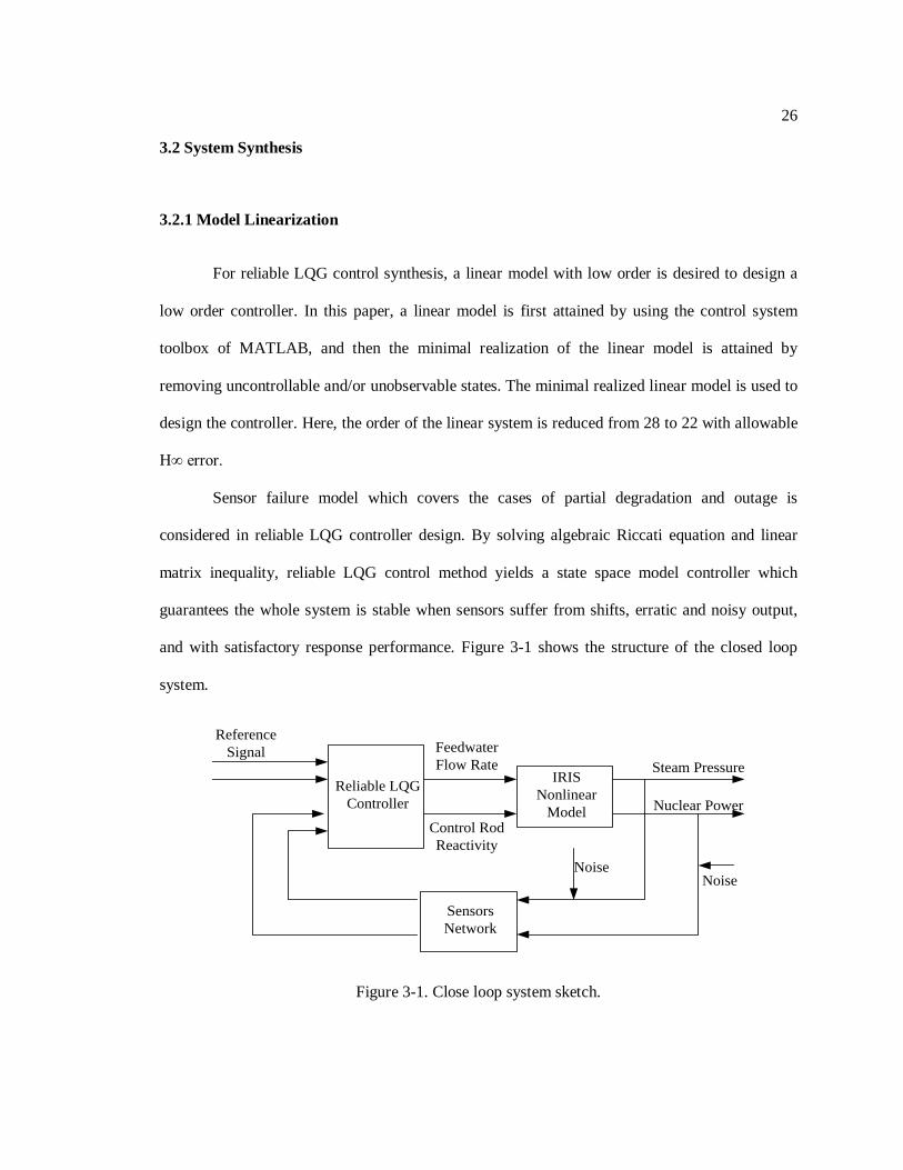
and with satisfactory response performance. Figure 3-1 shows the structure of the closed loop
system.
IRISNonlinear
Model
Reliable LQGController
SensorsNetwork
Feedwater Flow Rate
Control Rod Reactivity
Steam Pressure
Nuclear Power
ReferenceSignal
NoiseNoise
Figure 3-1. Close loop system sketch.
27
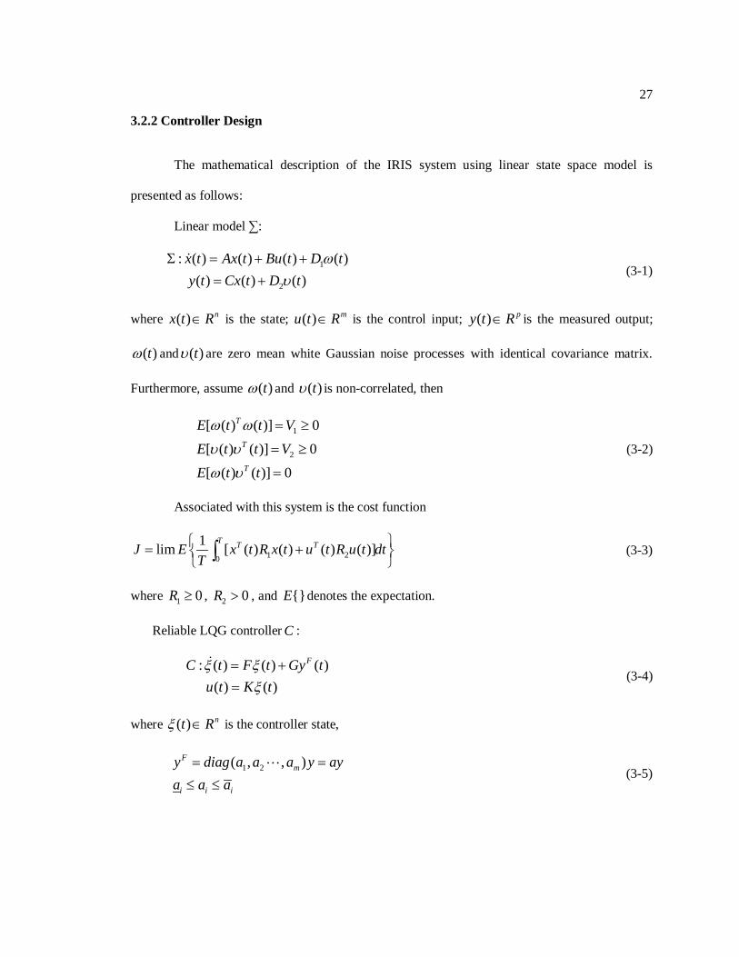
3.2.2 Controller Design
The mathematical description of the IRIS system using linear state space model is
presented as follows:
Linear model ∑:
1
2
: ( ) ( ) ( ) ( )( ) ( ) ( )
x t Ax t Bu t D ty t Cx t D t
ωυ
Σ = + += +
(3-1)
where ( ) nx t R∈ is the state; ( ) mu t R∈ is the control input; ( ) py t R∈ is the measured output;
( )tω and ( )tυ are zero mean white Gaussian noise processes with identical covariance matrix.
Furthermore, assume ( )tω and ( )tυ is non-correlated, then
1
2
[ ( ) ( )] 0
[ ( ) ( )] 0
[ ( ) ( )] 0
T
T
T
E t t VE t t VE t t
ω ω
υ υ
ω υ
= ≥
= ≥
=
(3-2)
Associated with this system is the cost function
1 20
1lim [ ( ) ( ) ( ) ( )]T T TJ E x t R x t u t R u t dt
T = + ∫ (3-3)
where 1 0R ≥ , 2 0R > , and E denotes the expectation.
Reliable LQG controller C :
: ( ) ( ) ( )( ) ( )
FC t F t Gy tu t K tξ ξ
ξ= +=
(3-4)
where ( ) nt Rξ ∈ is the controller state,
1 2( , , )Fm
i i i
y diag a a a y aya a a
= =≤ ≤
(3-5)
28
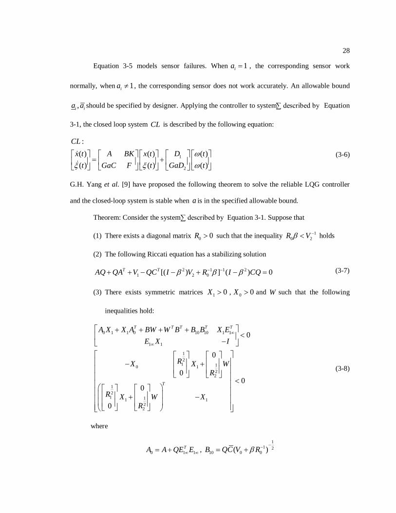
Equation 3-5 models sensor failures. When 1ia = , the corresponding sensor work
normally, when 1ia ≠ , the corresponding sensor does not work accurately. An allowable bound
,i ia a should be specified by designer. Applying the controller to system ∑ described by Equation
3-1, the closed loop system CL is described by the following equation:
1
2
:( ) ( ) ( )( ) ( ) ( )
CLDx t A BK x t t
GaDt GaC F t tω
ξ ξ ω
= +
(3-6)
G.H. Yang et al. [9] have proposed the following theorem to solve the reliable LQG controller
and the closed-loop system is stable when a is in the specified allowable bound.
Theorem: Consider the system ∑ described by Equation 3-1. Suppose that
(1) There exists a diagonal matrix 0 0R > such that the inequality 10 2R Vβ −< holds
(2) The following Riccati equation has a stabilizing solution
2 1 1 21 2 0[( ) ] ( ) 0T TAQ QA V QC I V R I CQβ β β− −+ + − − + − = (3-7)
(3) There exists symmetric matrices 1 0X > , 0 0X > and W such that the following
inequalities hold:
0 1 1 0 10 10 1 1
1 1
12
1 10 122
12
1 11 122
0
0
00
0
0
T T T T T
T
A X X A BW W B B B X EE X I
RX X WR
R X W XR
∞
∞
+ + + +< −
− + < + −
(3-8)
where
0 1 1TA A QE E∞ ∞= + ,
11 2
10 0 0( )B QC V Rβ−−= +

29
with
1 2
0 01 1
0 2 01 1 1 1 1 1 12 2 2 2 2 2 2
1 0 2 0 0
( , , )
( )
( )
( )
p
i ii
i i
diaga aa a
C I V R CV V R
E I R V R R C
β β β β
β
β
β
β β β
− −
−
∞
=
−=
+
= +
= −
= −
Then the corresponding reliable LQG controller is given by:
10 0 2 0
11
2 1 12 0 0
( )
[( ) ]T
F A Ga I V R C BKK WXG QC I V R a
β
β β
−
−
− −
= − − +
=
= − +
With
0 01 02 0( , , , )pa diag a a a=
The corresponding algorithm for the design given by this theorem is given as follows:
Step 1: Initialize 0R satisfying 10 2R Vβ −< and solve Equation 7 for Q .
Step 2: Minimize 0( )tr X subject to LMI constraints.
Step 3: If step 2 is not feasible, then change 0R and go to step 1.
This algorithm can be performed effectively by using MATLAB.
The controller obtained by this algorithm is with the same order as the plant. To make the
controller easy to realize, a reduced-order controller is desired. The same method which is used to
reduce the plant model is used to reduce the order of controller.

3.3 Simulation
According to the theorem given above, a reliable LQG controller which can be tolerant of
50%± sensors drift is designed. Applying the reliable LQG controller to the nonlinear system,
the following running condition is simulated:
Case I: at t=500s, the nuclear power reference signal steps from 100% nominal value to
90%, at t=800s, nuclear power reference signal steps from 90% to 100%, at t=1000s, nuclear
power sensor drifts 20% with slope of 1%/sec, at t=1500s, the sensor recovers from drift. Figure
3-2 shows the dynamic response of the closed loop system and Figure 3-3 shows the two control
effects: steam generator secondary side feedwater flow rate and control rod reactivity. In the
normal case, the controller can make the output of the nonlinear system follow the reference
signal with the steady state error less than 0.5%. The response time of nuclear power is 1sec.
When nuclear power sensors cannot provide accurate signals, the reliable LQG controller can still
maintain output-steam pressure reference signal with steady state error less than 1% and maintain
the system stable.
Figure 3-2.Dynamic response of case I.
0 200 400 600 800 1000 1200 1400 1600 18000.75
0.8
0.85
0.9
0.95
1
1.05
time/sec
outp
ut
Steam PressureNuclear Power

31
Figure 3-3.Control effects of case I.
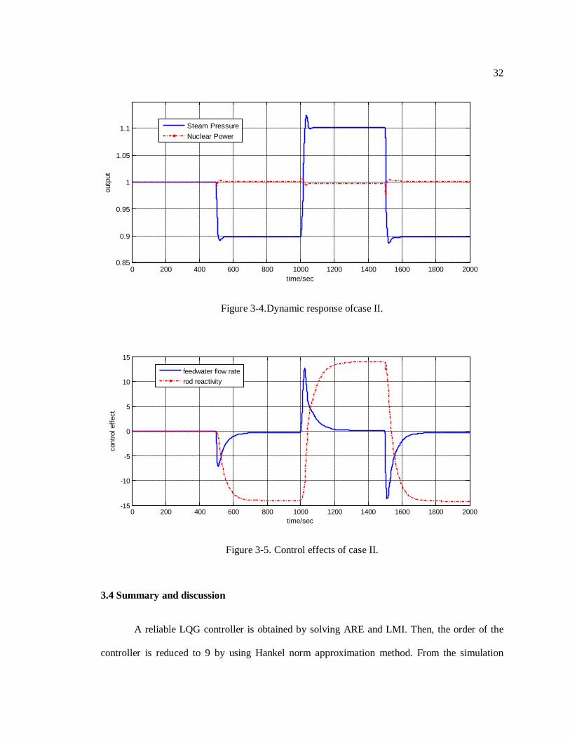
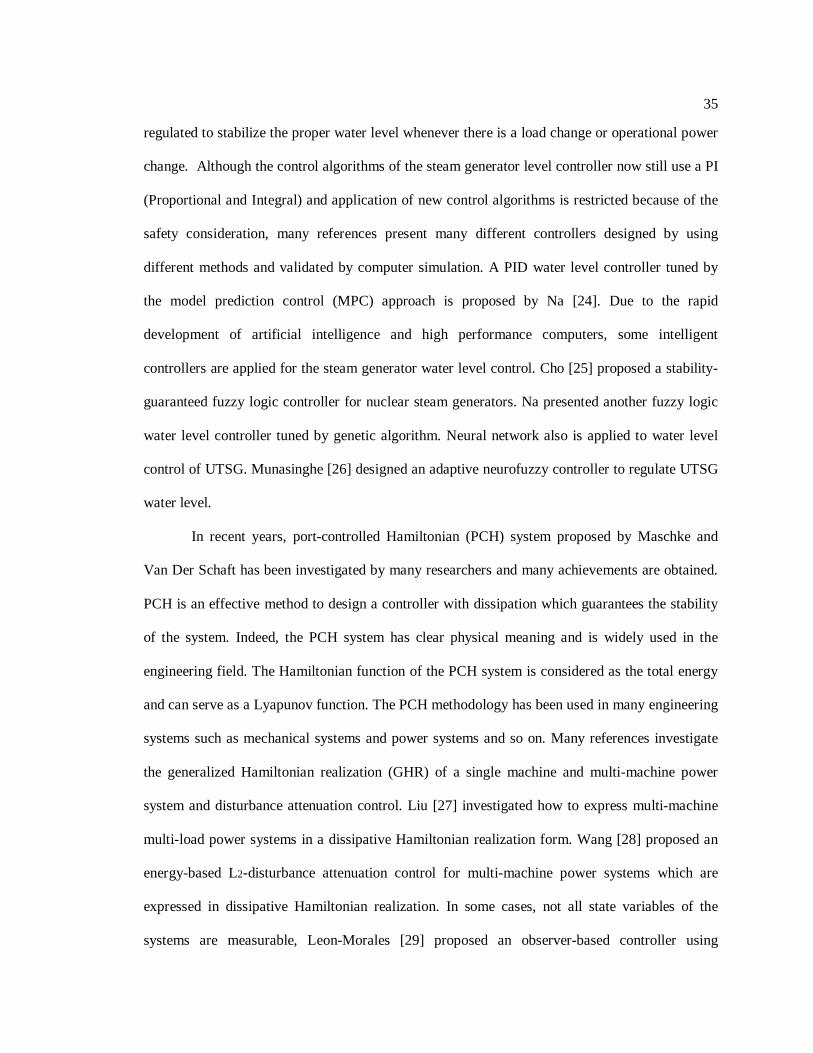
Case II: at t=500s, steam pressure reference signal step from 100% nominal value to
90%, at t=1000s, steam pressure sensor drifts 20% with slope of -1%/sec, at t=1500s, the sensor
recovers from the drift. Figure 3-4 shows the dynamic response of the closed-loop system and
Figure 3-5 shows the two control effects. Just like case I, in normal operation, the controller can
make the output of the nonlinear system follow the reference signal with the steady state error
less than 0.5%. The response time of steam pressure is 50 sec. When the steam pressure sensor
cannot provide an accurate signal, the reliable LQG controller can still maintain output-nuclear
power reference signal with steady state error less than 1% and maintain the system stable.
0 200 400 600 800 1000 1200 1400 1600 1800 2000-20
-15
-10
-5
0
5
time/sec
cont
rol e
ffect
feedwater flow raterod reactivity
32
Figure 3-4.Dynamic response ofcase II.
Figure 3-5. Control effects of case II.
3.4 Summary and discussion
A reliable LQG controller is obtained by solving ARE and LMI. Then, the order of the
controller is reduced to 9 by using Hankel norm approximation method. From the simulation
0 200 400 600 800 1000 1200 1400 1600 1800 20000.85
0.9
0.95
1
1.05
1.1
time/sec
outp
ut
Steam PressureNuclear Power
0 200 400 600 800 1000 1200 1400 1600 1800 2000-15
-10
-5
0
5
10
15
time/sec
cont
rol e
ffect
feedwater flow raterod reactivity

33
result, the LQG controller can maintain the system stable when sensors drift in allowable range
and perform well in tracking the reference signal. However, compared with robust control, for
example, H∞ robust control, the reliable LQG does not perform well in the noise rejection. So, the
future work will focus on enhancing the ability to reject noise of reliable LQG control.

Chapter 4
Nonlinear-Observed Feedback Dissipation Controller Design for HCSG Pressure Control
4.1 Introduction
The Steam Generators used in commercial pressurized water reactor power plants are U-
tube steam generators (UTSG) which are different than helical-coil steam generators (HCSG)
used in the IRIS system. For UTSG, water level control is one of the main control issues. To
guarantee the sufficient cooling of the nuclear reactor, and to avoid the damage of steam turbine
blades, the water level of steam generator should be maintained in a proper region, which is
important for the operational safety of the whole nuclear power plant system. Water level control
for UTSG is not easy to deal with. Several factors which lead to the difficulties in designing an
effective water level control system for UTSG were summarized by Kothare [23]. These factors
include: 1). the nonlinear plant characteristic arisen by the highly nonlinear plant dynamics; 2).
the nonminimum-phase plant characteristics arisen by the so called “swell and shrink” effects
[23]; 3). the unreliability of sensor measurement at low powers; 4). the constraints of the
feedwater flow rate arisen by the feedwater system. Meanwhile, the temperature and flow rate of
both primary loop coolant and secondary loop feedwater, the main steam flow rate have direct
effect on the water level. The main steam flow rate depends on the electrical load of the generator
while the temperature and flow rate of primary loop coolant depends on the operation power of
the nuclear reactor. So, the water level controller of the nuclear steam generator has feedwater
flow rate and temperature, coolant flow rate and temperature, and main steam flow rate as input.
It has the level control signal of the steam generator as output. The feedwater flow rate should be
35
regulated to stabilize the proper water level whenever there is a load change or operational power
change. Although the control algorithms of the steam generator level controller now still use a PI
(Proportional and Integral) and application of new control algorithms is restricted because of the
safety consideration, many references present many different controllers designed by using
different methods and validated by computer simulation. A PID water level controller tuned by
the model prediction control (MPC) approach is proposed by Na [24]. Due to the rapid
development of artificial intelligence and high performance computers, some intelligent
controllers are applied for the steam generator water level control. Cho [25] proposed a stability-
guaranteed fuzzy logic controller for nuclear steam generators. Na presented another fuzzy logic
water level controller tuned by genetic algorithm. Neural network also is applied to water level
control of UTSG. Munasinghe [26] designed an adaptive neurofuzzy controller to regulate UTSG
water level.
In recent years, port-controlled Hamiltonian (PCH) system proposed by Maschke and
Van Der Schaft has been investigated by many researchers and many achievements are obtained.
PCH is an effective method to design a controller with dissipation which guarantees the stability
of the system. Indeed, the PCH system has clear physical meaning and is widely used in the
engineering field. The Hamiltonian function of the PCH system is considered as the total energy
and can serve as a Lyapunov function. The PCH methodology has been used in many engineering
systems such as mechanical systems and power systems and so on. Many references investigate
the generalized Hamiltonian realization (GHR) of a single machine and multi-machine power
system and disturbance attenuation control. Liu [27] investigated how to express multi-machine
multi-load power systems in a dissipative Hamiltonian realization form. Wang [28] proposed an
energy-based L2-disturbance attenuation control for multi-machine power systems which are
expressed in dissipative Hamiltonian realization. In some cases, not all state variables of the
systems are measurable, Leon-Morales [29] proposed an observer-based controller using

36
Hamiltonian approach to control a synchronous generator. Generally, applying the Hamiltonian
function method to express the system concerned into a Hamiltonian system with dissipation
which is called dissipative Hamiltonian realization involves two steps. The first step is to express
the system into a generalized Hamiltonian system, i.e., obtain the GHR. The second step is to
eliminate the non-dissipative part of GHR by state feedback to get a Hamiltonian system with
dissipation. However, to express a system as a GHR, the output and the Hamiltonian function
should meet some matching conditions and furthermore it is not guaranteed that all of the state
variables are measurable, these two conditions make the controller design using Hamiltonian
function method difficult. To solve this problem, Dong [30][33] proposed a novel method called
observer-based feedback dissipation (OBFD) and then Dong used this OBFD theorem to design a
power controller for a low temperature nuclear reactor. OBFD is an effective method which can
express complicated nonlinear systems in the form of GHR. Another advantage of OBFD is that
controller design using OBFD method does not depend on the parameters of state functions
closely except the input matrix and output matrix which makes the design easier.
In this chapter, based on OBFD method, the pressure control of HCSG is considered.
HCSG which is used in the IRIS nuclear power plant is different than UTSG greatly in principle
and structure. Feedwater undergoes three different state regions: subcooled, boiling and
superheated after going into the helical-coil tube. There is not a “water level'” with clear physical
concept in HCSG. In other words, “water level” in HCSG is not measurable. Here “water level”
in HCSG is defined as the summation of the length of subcooled region and boiling region. The
control objective for the HCSG is to maintain the pressure of outlet steam to be a constant, while
maintaining the length of the three different state regions within acceptable boundaries.
OBFD is a model-based method. So in this chapter, a simple nonlinear state space model
for HCSG of IRIS is derived first according to basic energy balance and mass balance. Then

37
using OBFD method, a single input single output (SISO) pressure controller for HCSG is
designed. Simulation results show that the control performance is high.
4.2 Nonlinear State Space Model of HCSG
The steam turbine is an important and complicated component of a plant unit. For
different purpose, a specific mathematical model with different complexity should be built. Two
dynamic models are available for IRIS power plant systems which are developed by the North
Carolina State University [35] and the University of Tennessee [35]. Generally, these two models
consider a lot of detailed characteristics and consist of partial differential equations and ordinary
differential equations in which many state variables couple with each other. Usually, iterative
algorithms or finite difference methods are employed to solve the coupled differential equations.
The degree of the two models is higher than 20. All of these lead the two existing models to have
high fidelity and are suitable for the test and evaluation of a controller but not suitable for model-
based controller design.
Observer-based feedback dissipation (OBFD) is a model-based controller design method.
A simplified minimal dynamic state space model is needed. In this Chapter, based on the high
order mathematical model of HCSG[35] developed by University of Tennessee and a
mathematical model of UTSG[36] which is specified for nonlinear H∞ controller design, a
simplified low order lumped parameter model is developed and used to describe the HCSG
dynamic behavior. Each lump has the same averaged properties. This model is based on basic
mass and energy conservation and described by ordinary differential equations which are only
suitable for control system design. Because feedwater suffers three different states inside the
tubes of the secondary side of the HCSG which are subcooled water first, then two-phase boiling
steam and water mixture and finally superheated steam, correspondingly, three lumps are used to
38
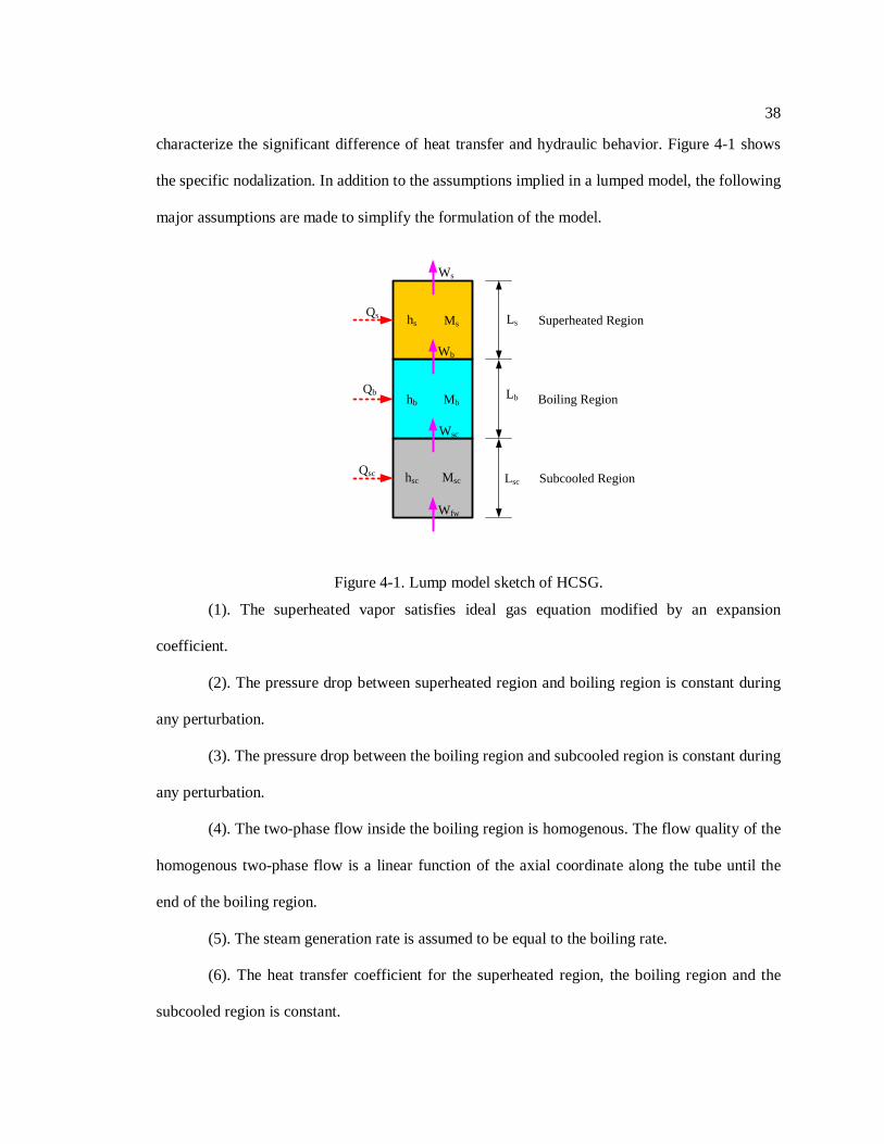
characterize the significant difference of heat transfer and hydraulic behavior. Figure 4-1 shows
the specific nodalization. In addition to the assumptions implied in a lumped model, the following
major assumptions are made to simplify the formulation of the model.
Qsc
Qb
Qs Ls
Lb
Lsc
Ws
Wb
Wfw
Wsc
hs
hsc
hb
Subcooled Region
Boiling Region
Superheated RegionMs
Mb
Msc
Figure 4-1. Lump model sketch of HCSG.
(1). The superheated vapor satisfies ideal gas equation modified by an expansion
coefficient.
(2). The pressure drop between superheated region and boiling region is constant during
any perturbation.
(3). The pressure drop between the boiling region and subcooled region is constant during
any perturbation.
(4). The two-phase flow inside the boiling region is homogenous. The flow quality of the
homogenous two-phase flow is a linear function of the axial coordinate along the tube until the
end of the boiling region.
(5). The steam generation rate is assumed to be equal to the boiling rate.
(6). The heat transfer coefficient for the superheated region, the boiling region and the
subcooled region is constant.
39
(7). The primary side of the HCSG is considered as a heat input.
Remark:
The real flow condition in the helical tube is complicated, especially in the two-phase
region. To reduce the order of the lumped state space model, Homogenous two-phase flow model
is considered here. Homogenous two-phase flow model is the simplest two-phase flow model
which makes it suitable for controller design. The linear steam quality with respect to the axial
coordinate along the tube until the end of the boiling region can be derived based on
homogeneous two-phase flow model.
Here, the nomenclature used to describe this nonlinear state space model is given in
Appendix A
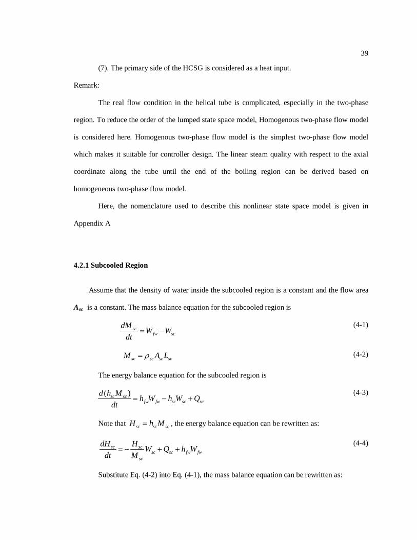
4.2.1 Subcooled Region
Assume that the density of water inside the subcooled region is a constant and the flow area
Asc
scfw sc
dM W Wdt
= −
is a constant. The mass balance equation for the subcooled region is
(4-1)
sc sc sc scM A Lρ= (4-2)
The energy balance equation for the subcooled region is
( )sc scfw fw sc sc sc
d h M h W h W Qdt
= − + (4-3)
Note that sc sc scH h M= , the energy balance equation can be rewritten as:
sc scsc sc fw fw
sc
dH H W Q h Wdt M
= − + + (4-4)
Substitute Eq. (4-2) into Eq. (4-1), the mass balance equation can be rewritten as:

40
fw scsc
sc sc
W WdLdt Aρ
−=
(4-5)
4.2.2 Boiling Region
The mass balance equation for the boiling region is
bsc g
dM W Wdt
= − (4-6)
b b b bM A Lρ= (4-7)
According to the assumption (4), the flow quality x of the homogenous two-phase flow
in the boiling region is a linear function of the length bL along the boiling region. At the
beginning of boiling region, x =0, at the end of the boiling region, x =1. This assumption yields
an average flow quality x⟨ ⟩ of the boiling region as
0.5x⟨ ⟩ = (4-8)
The energy balance equation for the boiling region is
( )b bsc sc g g b
d h M h W h W Qdt
= − + (4-9)
0.5b f fgh h h= + (4-10)
g f fgh h h= + (4-11)
Noticed that
b b b
b
d d dPdt dP dtρ ρ
= (4-12)
Substitute Eq. 4-7 and 4-12 into Eq. 4-6, the mass balance can be rewritten as:

41
bsc g b b b
b
b b
dPW W A L KdL dtdt A ρ
− −=
(4-13)
Where
bb
b
KPρ∂
=∂
(4-14)
In the operation pressure range, we have
( ) 1.61594 0.00552445b b bP Pρ = + (4-15)
According to Eq. 4-10, bh is a constant. Rewrite the Eq. 4-9 as
sc sc g g bb
b
h W h W QdMdt h
− +=
(4-16)
5.2.3 Superheated Region
The mass balance equation for the superheat region is
sg s
dM W Wdt
= − (4-17)
s s s sM A Lρ= (4-18)
The energy balance equation for the superheat region is
( )s s s ss g g s s s s
d M h PV Q W h W h PVdt
−= + − −
(4-19)
Since specific enthalpy is a function of temperature and pressure, then
s s ss s
s s
dh h hT Pdt T P
∂ ∂= +
∂ ∂
(4-20)
Combine Eq. 4-17, 4-18, 4-19 and 4-20 together, the energy balance equation can be
written as:
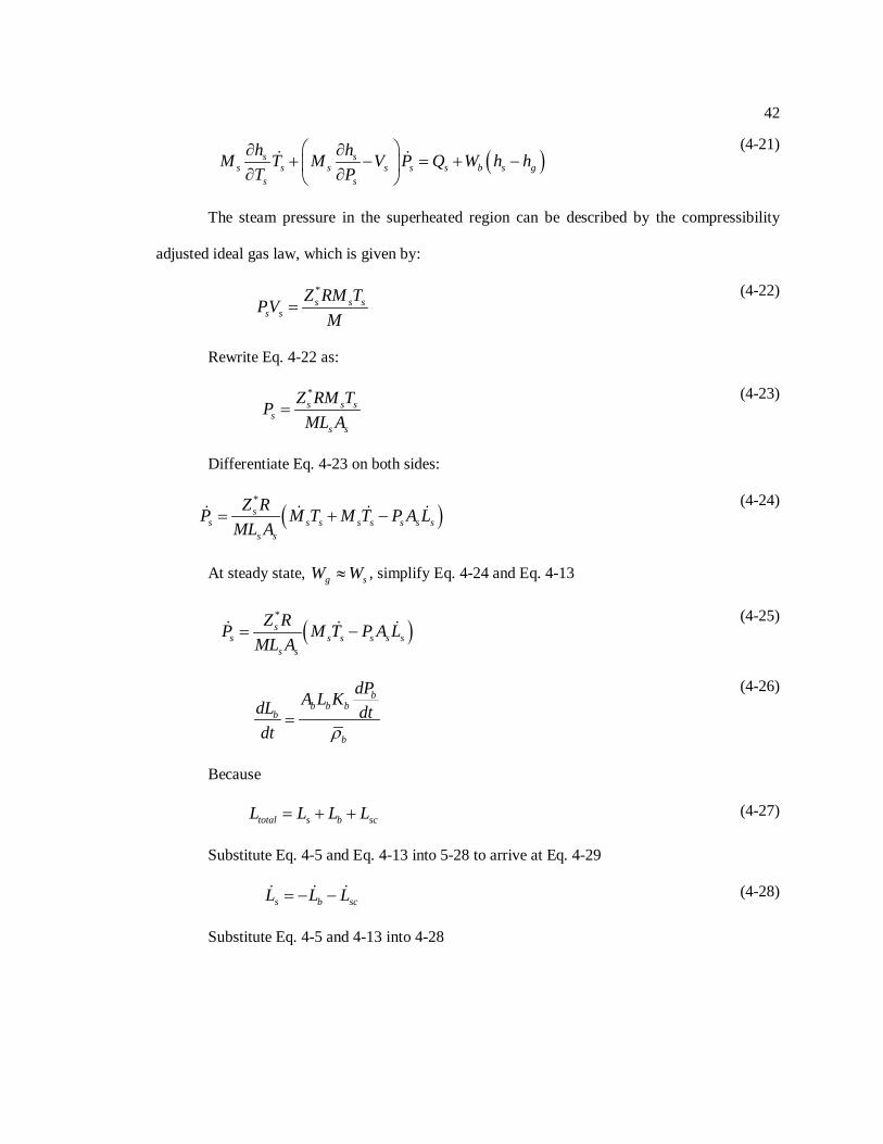
42
( )s ss s s s s s b s g
s s
h hM T M V P Q W h hT P
∂ ∂+ − = + − ∂ ∂
(4-21)
The steam pressure in the superheated region can be described by the compressibility
adjusted ideal gas law, which is given by:
*s s s
s sZ RM TPV
M=
(4-22)
Rewrite Eq. 4-22 as:
*s s s
ss s
Z RM TPML A
= (4-23)
Differentiate Eq. 4-23 on both sides:
( )*s
s s s s s s s ss s
Z RP M T M T P A LML A
= + − (4-24)
At steady state, g sW W≈ , simplify Eq. 4-24 and Eq. 4-13
( )*s
s s s s s ss s
Z RP M T P A LML A
= − (4-25)
bb b b
b
b
dPA L KdL dtdt ρ
=
(4-26)
Because
total s b scL L L L= + + (4-27)
Substitute Eq. 4-5 and Eq. 4-13 into 5-28 to arrive at Eq. 4-29
s b scL L L= − − (4-28)
Substitute Eq. 4-5 and 4-13 into 4-28
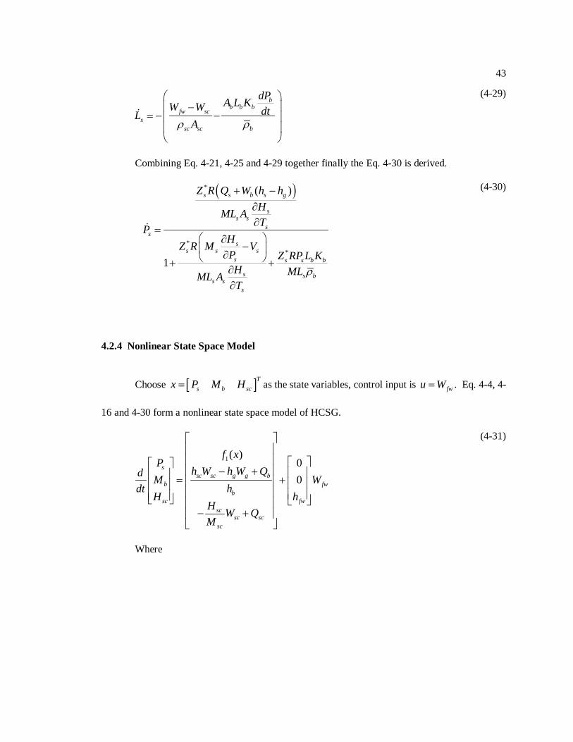
43
bb b b
fw scs
sc sc b
dPA L KW W dtLAρ ρ
−
= − −
(4-29)
Combining Eq. 4-21, 4-25 and 4-29 together finally the Eq. 4-30 is derived.
( )*
**
( )
1
s s b s g
ss s
ss
ss s s
s s s b b
s s bs s
s
Z R Q W h hHML ATP
HZ R M VP Z RP L KH MLML AT
ρ
+ −∂∂
= ∂
− ∂ + +∂∂
(4-30)
4.2.4 Nonlinear State Space Model
Choose [ ]Ts b scx P M H= as the state variables, control input is fwu W= . Eq. 4-4, 4-
16 and 4-30 form a nonlinear state space model of HCSG.
1( )00
ssc sc g g b
b fwb
sc fwsc
sc scsc
f xP
h W h W Qd M Wdt h
H hH W QM
− + = +
− +
(4-31)
Where
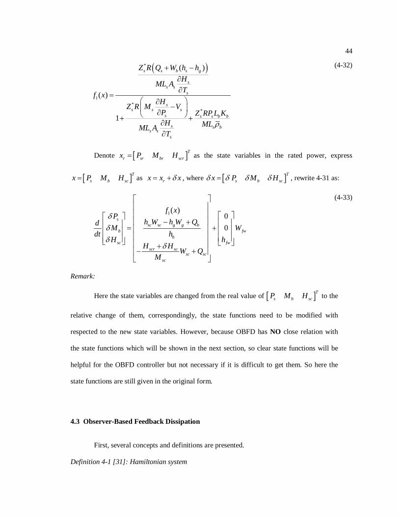
44
( )*
1*
*
( )
( )
1
s s b s g
ss s
s
ss s s
s s s b b
s s bs s
s
Z R Q W h hHML ATf x
HZ R M VP Z RP L KH MLML AT
ρ
+ −∂∂
= ∂
− ∂ + +∂∂
(4-32)
Denote [ ]Tr sr br scrx P M H= as the state variables in the rated power, express
[ ]Ts b scx P M H= as rx x xδ= + , where [ ]T
s b scx P M Hδ δ δ δ= , rewrite 4-31 as:
1( )00
ssc sc g g b
b fwb
sc fwscr sc
sc scsc
f xP
h W h W Qd M Wdt h
H hH H W Q
M
δδδ
δ
− + = + +− +
(4-33)
Remark:
Here the state variables are changed from the real value of [ ]Ts b scP M H to the
relative change of them, correspondingly, the state functions need to be modified with
respected to the new state variables. However, because OBFD has NO close relation with
the state functions which will be shown in the next section, so clear state functions will be
helpful for the OBFD controller but not necessary if it is difficult to get them. So here the
state functions are still given in the original form.
4.3 Observer-Based Feedback Dissipation
First, several concepts and definitions are presented.
Definition 4-1 [31]: Hamiltonian system

45
An autonomous dynamic system
( ) nR∈ x = f x , x (4-34)
with 0( ) =f x 0 for some 0nR∈x , is called a generalized Hamiltonian system (GHS) if the
dynamic system expressed by Eq. 4-34 can be expressed as
( ) ( )H∇x = T x x (4-35)
Where ( ) n nR ×∈T x is a real matrix that is called the structure matrix and ( ) : nH R R+• →
( [0, ))R+ = ∞ , is a smooth function, and is called the Hamiltonian function, represents the
total stored energy, and
( )( )THH ∂ ∇ = ∂
xxx
Where
1 2
( ) ( ) ( ) ( ), , ,n
H H H Hx x x
∂ ∂ ∂ ∂= ∂ ∂ ∂ ∂
x x x x
x
Based on the Definition 4-1, the concept of dissipative system is given as follows
Definition 4-2
If the structure matrix
[31]: Hamiltonian realization
( )T x of the dynamic Eq. 4-35 can be expressed as
( )= ( ) ( )−T x J x R x with skew-symmetric ( )J x and symmetric nonnegative ( )R x , then
system Eq. 4-34 is said to be dissipative, and Eq. 4-35 is the dissipative generalized
Hamiltonian realization of the system in Eq. 4-34. Moreover, the system in Eq. 4-34 is said
to be strict dissipative if ( )R x is positive, and Eq. 4-35 is the corresponding strict dissipative
generalized Hamiltonian realization.
From Eq. 4-31, the nonlinear dynamics of the HCSG is essentially a sample of the single-
input-single-output (SISO) nonlinear systems taking the form as
46
( ) ( )( )
uy h
+ =
x = f x g xx
(4-36)
Where nR∈x is the state vector, u R∈ is the control input and y R∈ is the output. To express
anonlinear system taking the form of Eq. 4-36 as a generalized Hamiltonian function, an
important and useful lemma is given as follows:
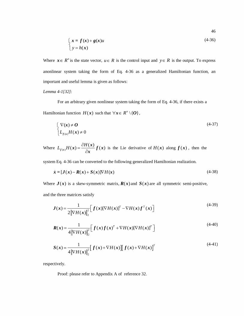
Lemma 4-1[32]:
For an arbitrary given nonlinear system taking the form of Eq. 4-36, if there exists a
Hamiltonian function ( )H x such that \ nR∀ ∈x O ,
( )
( )( ) 0L H
∇ ≠ ≠ f x
x O x
(4-37)
Where ( )( )( ) ( )HL H ∂
=∂f x
xx f xx
is the Lie derivative of ( )H x along ( )f x , then the
system Eq. 4-36 can be converted to the following generalized Hamiltonian realization.
[ ( ) ( ) ( )] ( )H− + ∇x = J x R x S x x (4-38)
Where ( )J x is a skew-symmetric matrix, ( )R x and ( )S x are all symmetric semi-positive,
and the three matrices satisfy
2
2
1( ) ( )[ ( )] ( ) ( )2 ( )
T TH HH
= ∇ − ∇ ∇J x f x x x f x
x
(4-39)
2
2
1( ) ( ) ( ) ( )[ ( )]4 ( )
T TH HH
= + ∇ ∇ ∇R x f x f x x x
x
(4-40)
[ ][ ]2
2
1( ) ( ) ( ) ( ) ( )4 ( )
TH HH
= + ∇ + ∇∇
S x f x x f x xx
(4-41)
respectively.
Proof: please refer to Appendix A of reference 32.
47
From Lemma 4-1, the generalized Hamiltonian realization for the nonlinear state-space of
HCSG Eq. 4-31 can be written as
[ ( ) ( ) ( )] ( )+ ( )
( )
d H udty h
− + ∇
=
x = J x R x S x x g x
x
(4-42)
Where x is the state variable, u R∈ is the control input, ( ) Th =x c x , ( )H x is the Hamiltonian
function which is chosen as
21( )2 sH Pδ=x
(4-43)
( )J x , ( )R x and ( )S x satisfy Eq. 4-39, 4-40, 4-41 respectively. Usually, to get the generalized
Hamiltonian system, a matching condition between output and Hamiltonian function should be
satisfied which is:
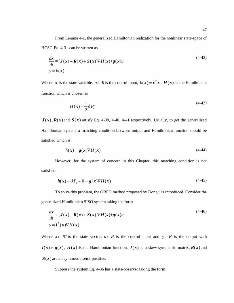
( ) ( ) ( )h H= ∇x g x x (4-44)
However, for the system of concern in this Chapter, this matching condition is not
satisfied:
( ) 0 ( ) ( )sh P Hδ= ≠ = ∇x g x x (4-45)
To solve this problem, the OBFD method proposed by Dong10
[ ( ) ( ) ( )] ( )+ ( )
( ) ( )T
d H udty H
− + ∇
= ∇
x = J x R x S x x g x
l x x
is introduced. Consider the
generalized Hamiltonian SISO system taking the form
(4-46)
Where nR∈x is the state vector, u R∈ is the control input and y R∈ is the output with
( ) ( )≠l x g x , ( )H x is the Hamiltonian function. ( )J x is a skew-symmetric matrix, ( )R x and
( )S x are all symmetric semi-positive.
Suppose the system Eq. 4-36 has a state-observer taking the form
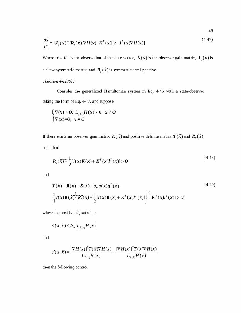
48
ˆ ˆˆˆˆˆˆ[ ( ) ( )] ( )+ ( )[ ( ) ( )]T Td H y Hdt
− ∇ − ∇0 0x = J x R x x K x l x x
(4-47)
Where ˆ nR∈x is the observation of the state vector, ˆ( )K x is the observer gain matrix, ˆ( )0J x is
a skew-symmetric matrix, and ˆ( )0R x is symmetric semi-positive.
Theorem 4-1[30]:
Consider the generalized Hamiltonian system in Eq. 4-46 with a state-observer
taking the form of Eq. 4-47, and suppose
( )( ) ( ) 0, ( )=
L H∇ ≠ ≠ ≠∇
f xx O, x x O x O, x = O
If there exists an observer gain matrix ˆ( )K x and positive definite matrix ˆ( )T x and ˆ( )0R x
such that
1ˆˆˆˆˆ( ) [ ( ) ( ) ( ) ( )]2
T T+ + >0R x l x K x K x l x O (4-48)
and
1
ˆ( ) ( ) ( ) ( ) ( )
1 1ˆˆˆˆˆˆˆˆ( ) ( ) ( ) [ ( ) ( ) ( ) ( )] ( ) ( )]4 2
Tm
T T T T
δ−
+ − − −
+ + >
0
T x R x S x g x g x
l x K x R x l x K x K x l x K x l x O
(4-49)
where the positive mδ satisfies:
( )ˆ( , ) ( )m L Hδ δ≤ f xx x x
and
ˆ( ) ( )
ˆˆˆˆ[ ( )] ( ) ( ) [ ( )] ( ) ( )ˆ( , )ˆ( ) ( )
T TH H H HL H L H
δ ∇ ∇ ∇ ∇= −
f x f x
x T x x x T x xx xx x
then the following control

49
ˆ( )
ˆˆˆ[ ( )] ( ) ( )ˆ( )ˆ( )
TH HuL H
∇ ∇= −
f x
x T x xxx
guarantee asymptotically stability of the close-loop systems.
Proof: please see reference 30
Remark:
If the state functions are simple, ( )R x and ( )S x can be calculated directly, then
by solving the matrix inequality Eq. 4-48 and Eq. 4-49, the OBFD controller is obtained
directly. If the state functions are very complicated, whose ( )R x and ( )S x can not
computed easily and obtained directly, then the parameters of the observer usually are
obtained by experience and validated by simulation for such a complicated system.
5.4 Simulation and Result
The OBFD dissipative controller is applied to stabilize the pressure of the outlet steam of
the HCSG. The HCSG model is developed by University of Tennessee using SIMULINK. This
whole IRIS model consists of a 22nd order HCSG, a 2nd
ˆ( )0J x
order point kinetics with one delayed
neutron group, and 4th order heat exchange of reactor core with temperature feedback from
lumped fuel and coolant temperature calculation [34] which were added at the Pennsylvania State
University.
, ˆ( )0R x , ˆ( )K x and ˆ( )T x is chosen as
50
ˆ( )
0 1 0ˆ( ) 1 0 0 ,
0 0 0ˆ( ) 10,ˆ( ) [1000 0 0], ˆˆ( ) ( )L H
= −
==
=
0
0
f x
J x
R xK x
T x x
The following conditions are simulated:
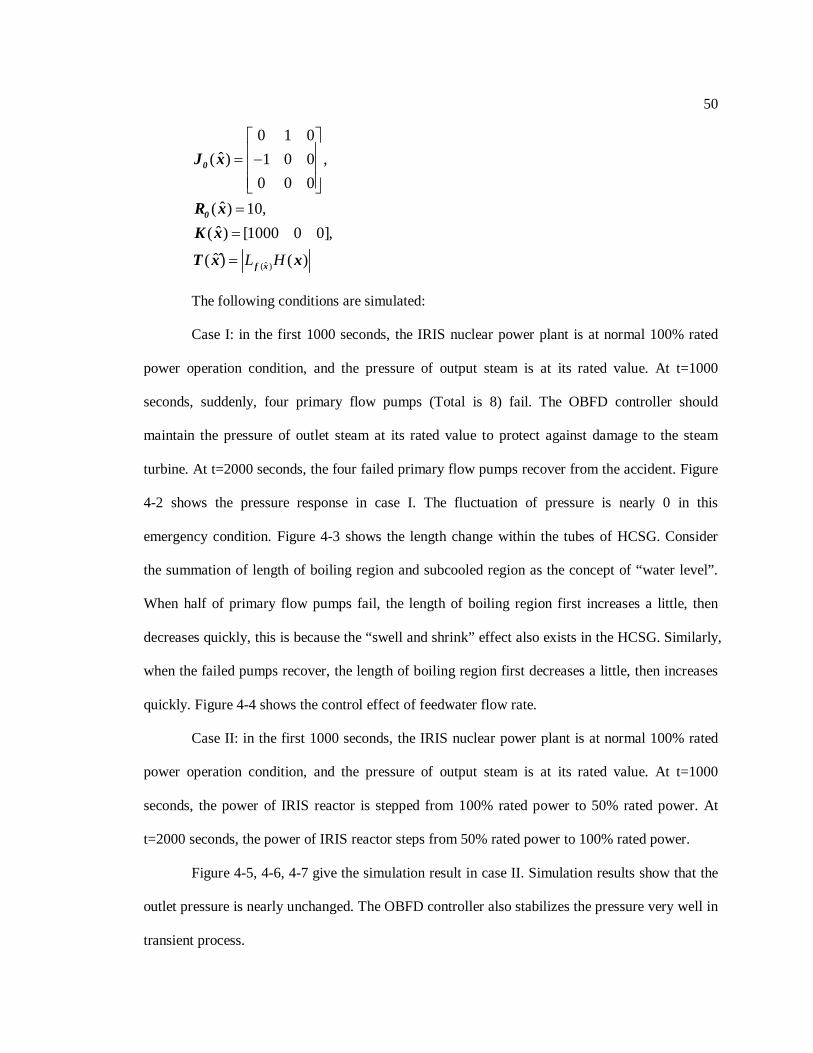
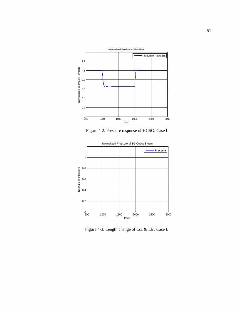
Case I: in the first 1000 seconds, the IRIS nuclear power plant is at normal 100% rated
power operation condition, and the pressure of output steam is at its rated value. At t=1000
seconds, suddenly, four primary flow pumps (Total is 8) fail. The OBFD controller should
maintain the pressure of outlet steam at its rated value to protect against damage to the steam
turbine. At t=2000 seconds, the four failed primary flow pumps recover from the accident. Figure
4-2 shows the pressure response in case I. The fluctuation of pressure is nearly 0 in this
emergency condition. Figure 4-3 shows the length change within the tubes of HCSG. Consider
the summation of length of boiling region and subcooled region as the concept of “water level”.
When half of primary flow pumps fail, the length of boiling region first increases a little, then
decreases quickly, this is because the “swell and shrink” effect also exists in the HCSG. Similarly,
when the failed pumps recover, the length of boiling region first decreases a little, then increases
quickly. Figure 4-4 shows the control effect of feedwater flow rate.
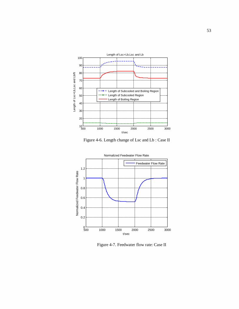
Case II: in the first 1000 seconds, the IRIS nuclear power plant is at normal 100% rated
power operation condition, and the pressure of output steam is at its rated value. At t=1000
seconds, the power of IRIS reactor is stepped from 100% rated power to 50% rated power. At
t=2000 seconds, the power of IRIS reactor steps from 50% rated power to 100% rated power.
Figure 4-5, 4-6, 4-7 give the simulation result in case II. Simulation results show that the
outlet pressure is nearly unchanged. The OBFD controller also stabilizes the pressure very well in
transient process.
51
Figure 4-2. Pressure response of HCSG: Case I
Figure 4-3. Length change of Lsc & Lb : Case I.
500 1000 1500 2000 2500 30000
0.2
0.4
0.6
0.8
1
1.2
t/sec
Nor
mal
ized
Fee
dwat
er F
low
Rat
e
Normalized Feedwater Flow Rate
Feedwater Flow Rate
500 1000 1500 2000 2500 30000
0.2
0.4
0.6
0.8
1
t/sec
Nor
mal
ized
Pre
ssur
e
Normalized Pressure of SG Outlet Steam
Pressure

52
Figure 4-4. Feedwater flow rate : Case I
Figure 4-5. Pressure response of HCSG: Case II
500 1000 1500 2000 2500 300010
20
30
40
50
60
70
80
90
100
t/sec
Leng
th o
f Lsc
+Lb,
Lsc
and
Lb/ft
Length of Lsc+Lb,Lsc and Lb
Length of Subcooled and Boiling RegionLength of Subcooled RegionLength of Boiling Region
500 1000 1500 2000 2500 30000
0.2
0.4
0.6
0.8
1
1.2
t/sec
Nor
mal
ized
Fee
dwat
er F
low
Rat
e
Normalized Feedwater Flow Rate
Feedwater Flow Rate
53
Figure 4-6. Length change of Lsc and Lb : Case II
Figure 4-7. Feedwater flow rate: Case II
500 1000 1500 2000 2500 300010
20
30
40
50
60
70
80
90
100
t/sec
Leng
th o
f Lsc
+Lb,
Lsc
and
Lb/ft
Length of Lsc+Lb,Lsc and Lb
Length of Subcooled and Boiling RegionLength of Subcooled RegionLength of Boiling Region
500 1000 1500 2000 2500 30000
0.2
0.4
0.6
0.8
1
1.2
t/sec
Nor
mal
ized
Fee
dwat
er F
low
Rat
e
Normalized Feedwater Flow Rate
Feedwater Flow Rate

54
4.5 Summary
Stabilization of pressure of the outlet steam in the HCSG is important for operation and
safety of the IRIS nuclear power plant. Using the level control of current U-tube steam generator
for reference, a nonlinear observer-based feedback dissipation controller for the pressure control
of HCSG is presented in this chapter. The first step of the OBFD is to model the HCSG in the
form of a simplified nonlinear state space model, and then based-on this simplified model, OBFD
is designed. Numerical simulation is done by applying the OBFD to a SIMULINK IRIS model
which is higher order. The simulation results show that the OBFD can well stabilize the pressure
of HCSG.
Furthermore, because the state space model used to design the OBFD controller is simple
and with low order, Uncertainties are introduced in the process of model simplification. So an
OBFD with large stable margin is expected. If ( )R x and ( )S x can be calculated directly, then
by solving the matrix inequality Eq. 4-48 and Eq. 4-49, and choosing a sufficient positive solution,
the OBFD controller is obtained directly and can guarantee enough stable margin. But usually, for
a complicated system, the matrix of ( )R x and ( )S x can not be calculated directly, then the
matrix of the observer can only be obtained by experience and validated by simulation. That is
the limitation of the OBFD.
55
Chapter 5
Online State Observer Design Based on Dissipation-Based High Gain Filter
5.1 Introduction
The control and operation of complex systems, such as nuclear power plants, critically
rely on monitoring of the state variables. Knowing the system states is necessary to solve many
control theory problems, for example, stabilizing a system using state feedback. Usually, sensor
systems are applied to sample and monitor the system state variables, for example, temperature,
pressure. Unfortunately, in most practical cases, many physical states of the system cannot be
determined by direct observation, i.e. the fuel temperature of reactor core, the concentration of
delayed neutrons, while in some cases, some state variables cannot be interpreted as explicit
physical variables. To solve this problem, state observers are built to reconstruct some desired
states which are unmeasurable. State observer is a system that models a real system in order to
provide an estimate of its internal state, given measurements of the input and output of the real
system. It is typically a computer-implemented mathematical model. The observer is called
asymptotically stable if the estimated states converge to the real state when the time goes to
infinity. For linear system, the Kalman filter (KF) is the most widely used state observer in
practical engineering [38]. Specifically, in nuclear engineering field, the application of KF in
monitoring and fault detection and isolation (FDI) for nuclear reactor is also done [39][40][41].
However, since nuclear power plant systems are highly nonlinear, the KF filter cannot achieve an
acceptable performance. State observer for nonlinear system is needed. For a nonlinear system,
the state observer design is more complicated than that for a linear system. The observer design
56
for a nonlinear system has been an active research topic for decades. In general, there are two
main approaches [51]. In the first approach [42][43][44], nonlinear systems are brought into a so-
called observer form by means of a nonlinear state transformation. This special form yields a
completely linear error dynamic of state such that linear observer theory can be applied.
However, for this approach, the condition for achieving the desired state coordinate
transformation are in general difficult to satisfy, which requires the solution of a set of partial
differential equations. More recently, significant research efforts have been directed to alleviate
the difficulty by developing more generalized state transformation procedures and more
generalized canonical forms so that the larger class of nonlinear system can be dealt with
[45][46]. On the other hand, the second approach is concerned with designing observer for
nonlinear system without the need of state transformation. The high-gain observers in
[47][48][49][50] are attractive because of their robustness. Available design techniques include
pole-placement approach [47], Riccati equation approach [48], Lyapunov equation approach [49]
and dissipation approach [50].
In this chapter, a nonlinear observer for the IRIS reactor is realized based on the
dissipation-based high gain filter (DHGF) theory proposed by Dong [50]. Some basic concepts
about dissipation theory and Hamiltonian realization are introduced in Chapter 4. These concepts
will be recalled here to design the state-observer.
5.2 Methodology
5.2.1 Problem Formulation
Consider the nonlinear systems taking the form as [50]
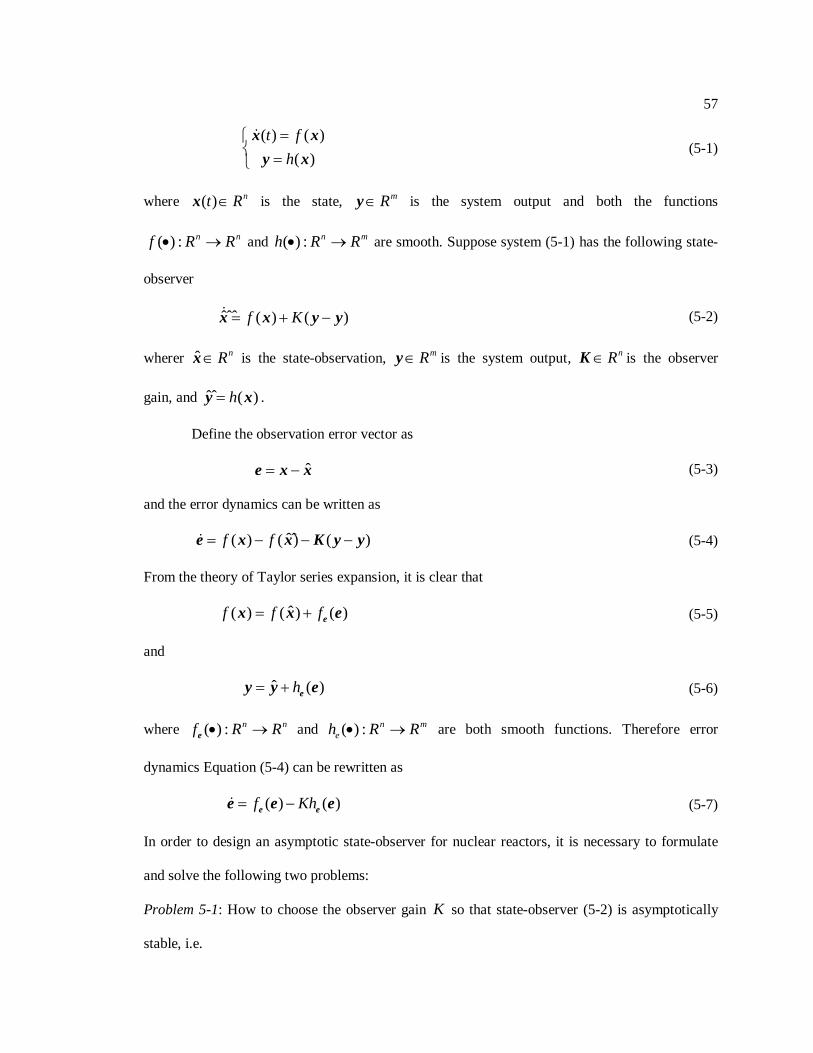
57
( ) ( )( )
t fh
= =
x xy x
(5-1)
where ( ) nt R∈x is the state, mR∈y is the system output and both the functions
( ) : n nf R R• → and ( ) : n mh R R• → are smooth. Suppose system (5-1) has the following state-
observer
ˆˆˆ ( ) ( )f K= + −x x y y (5-2)
wherer ˆ nR∈x is the state-observation, mR∈y is the system output, nR∈K is the observer
gain, and ˆˆ ( )h=y x .
Define the observation error vector as
ˆ= −e x x (5-3)
and the error dynamics can be written as
ˆˆ( ) ( ) ( )f f= − − −e x x K y y (5-4)
From the theory of Taylor series expansion, it is clear that
ˆ( ) ( ) ( )f f f= + ex x e (5-5)
and
ˆ ( )h= + ey y e (5-6)
where ( ) : n nf R R• →e and ( ) : n meh R R• → are both smooth functions. Therefore error
dynamics Equation (5-4) can be rewritten as
( ) ( )f Kh= − e ee e e (5-7)
In order to design an asymptotic state-observer for nuclear reactors, it is necessary to formulate
and solve the following two problems:
Problem 5-1: How to choose the observer gain K so that state-observer (5-2) is asymptotically
stable, i.e.

58
limt
o→∞
=e
The actual dynamics of nuclear reactors is very complex, and the mathematical model used in
controller design for nuclear reactor can only approximately describe the actual reactor dynamics
near some given operating point. There must be exterior disturbances and model uncertainty, and
then it is quite necessary to solve the following problem 2:
Problem 5-2: How to evaluate the robustness of the state-observer?
5.2.1 Design and Robustness Analysis of DHGF
In order to present the design of the DHGF, the concept of zero-state detectability is
introduced as follows:
Definition 5-1[52]: Consider the nonlinear systems taking the form as
( )( )
ξ ξη ξ
= Φ
= Θ
(5-8)
where and nRξ ∈ is the state-vector, mRη ∈ is the system output, and both the functions
( ) : n nR RΦ • → and ( ) : n mR RΘ • → are smooth functions. System 5-8 is called zero-state
detectable if ( 0)tη = ∀ ≥o implies limt
oξ→∞
= .
Based on the definition of zero-state observability, Theorem 5-1 is given as follows,
which gives the solution of Problem 5-1.
Theorem 5-1: Consider the nonlinear systems described by dynamic 5-1 with state-observer
taking the form as Equation 5-2. Define
ˆ=ye y - y (5-9)
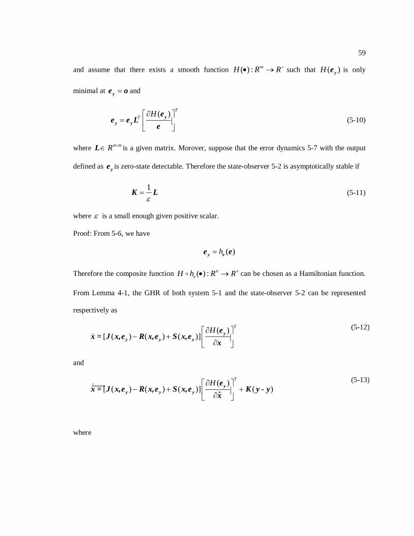
59
and assume that there exists a smooth function ( ) : mH R R+• → such that ( )H ye is only
minimal at =ye o and
( ) TT H∂
=
yy y
ee e L
e (5-10)
where n mR ×∈L is a given matrix. Morover, suppose that the error dynamics 5-7 with the output
defined as ye is zero-state detectable. Therefore the state-observer 5-2 is asymptotically stable if
1ε
=K L (5-11)
where ε is a small enough given positive scalar.
Proof: From 5-6, we have
( )h=y ee e
Therefore the composite function ( ) : neH h R R+• → can be chosen as a Hamiltonian function.
From Lemma 4-1, the GHR of both system 5-1 and the state-observer 5-2 can be represented
respectively as
( )[ ( ) ( ) ( )]
TH∂ − + ∂
yy y y
ex = J x,e R x,e S x,e
x
(5-12)
and
( )ˆˆˆˆ[ ( ) ( ) ( )] ( )
ˆ
TH∂ − + + ∂
yy y y
ex = J x,e R x,e S x,e K y - y
x
(5-13)
where
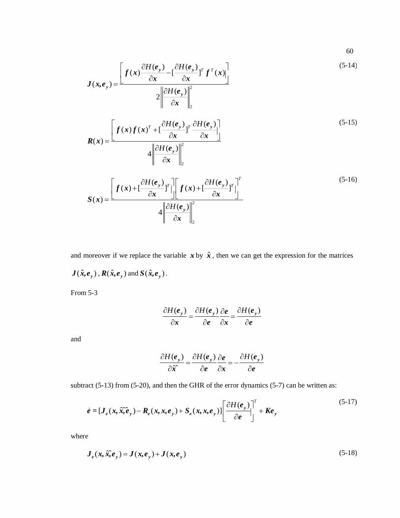
60
2
2
( ) ( )( ) [ ] ( )
( )( )
2
T TH H
H
∂ ∂ − ∂ ∂ =
∂∂
y y
yy
e ef x f x
x xJ x,e
ex
(5-14)
2
2
( ) ( )( ) ( ) [ ]
( )( )
4
T TH H
H
∂ ∂ + ∂ ∂ =∂
∂
y y
y
e ef x f x
x xR x
ex
(5-15)
2
2
( ) ( )( ) [ ] ( ) [ ]
( )( )
4
TT TH H
H
∂ ∂ + + ∂ ∂ =
∂∂
y y
y
e ef x f x
x xS x
ex
(5-16)
and moreover if we replace the variable x by x , then we can get the expression for the matrices
ˆ( )yJ x,e , ˆ( )yR x,e and ˆ( )yS x,e .
From 5-3
( ) ( ) ( )H H H∂ ∂ ∂∂= =
∂ ∂ ∂ ∂y y ye e ee
x e x e
and
( ) ( ) ( )ˆˆ
H H H∂ ∂ ∂∂= = −
∂ ∂ ∂ ∂y y ye e ee
x e x e
subtract (5-13) from (5-20), and then the GHR of the error dynamics (5-7) can be written as:
( )ˆˆˆ[ ( ) ( ) ( )]
TH∂ − + + ∂
ye y e y e y y
ee = J x, x,e R x, x,e S x, x,e Ke
e
(5-17)
where
ˆˆ( ) ( ) ( )= +e y y yJ x, x,e J x,e J x,e (5-18)
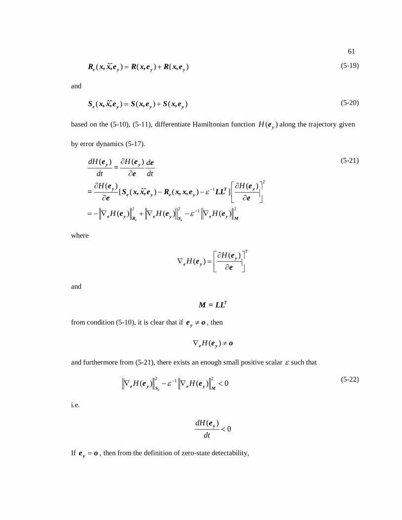
61
ˆˆ( ) ( ) ( )= +e y y yR x, x,e R x,e R x,e (5-19)
and
ˆˆ( ) ( ) ( )= +e y y yS x, x,e S x,e S x,e (5-20)
based on the (5-10), (5-11), differentiate Hamiltonian function ( )H ye along the trajectory given
by error dynamics (5-17).
1
2 2 21
( ) ( )
( ) ( )ˆˆ[ ( ) ( ) ]
( ) ( ) ( )
T
dH H ddt dtH H
H H H
ε
ε
−
−
∂
∂
∂ ∂ − − ∂ ∂
= − ∇ + ∇ − ∇e e
y y
y yTe y e y
e y e y e yR S M
e e e=e
e e= S x, x,e R x, x,e LL
e e
e e e
(5-21)
where
( )( )
THH
∂ ∇ = ∂
ye y
ee
e
and
TM = LL
from condition (5-10), it is clear that if ≠ye o , then
( )H∇ ≠e ye o
and furthermore from (5-21), there exists an enough small positive scalar ε such that
2 21( ) ( ) 0H Hε −∇ − ∇ <e
e y e yS Me e (5-22)
i.e.
( )0
dHdt
<ye
If =ye o , then from the definition of zero-state detectability,

62
limt→∞
=e o
Therefore if conditions (5-10) and (5-11) are both satisfied, then the state-observer (5-2) is
asymptotically stable for small enough positive scalar ε .
The robustness analysis of the DHGF is given in the reference [50].
5.3 Application in IRIS Nuclear Power Plant
5.3.1 State Space Model of IRIS Core for State-Observer Design
In this section, the DHGF for monitoring the IRIS reactor state will be realized. The
dynamic model which is used to design the DHGF is based on Equations (2-1) and (2-2).
Generally, to make the estimation more accurate, the corresponding dynamic model should give
more information about the real physical process. However, since the dynamic model which is
used to design the DHGF should satisfy some requirements such as zero-state detectability and
note that some lower-order models also give acceptable and reasonable description for the
dynamic process, so here, some reasonable simplifications are made. Note that the one-delayed
neutron group is essentially an equivalent delayed neutron group whose concentration and decay
constant are both the average values of those corresponding to the six delayed neutron group, so
the one delayed neutron group point kinetic is used here. Then, treat the a whole fuel rod as a cell,
the dynamic model which is used for DHGF design is given as:
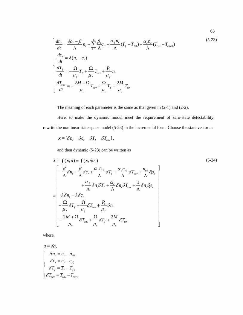
63
6
0 01
0
( ) ( )
( )
f ri c rr rr ri f f cav cav
i
rr r
ff cav r
f f f
n ndn n c T T T Tdtdc n cdt
dT PT T ndt
αβ αδρ β
λ
µ µ µ
=
−= + + − + −
Λ Λ Λ Λ
= −
Ω Ω= − + +
∑
2 2 cavcav f cin
c c c
dT M MT T Tdt µ µ µ
+ Ω Ω = − + +
(5-23)
The meaning of each parameter is the same as that given in (2-1) and (2-2).
Here, to make the dynamic model meet the requirement of zero-state detectability,
rewrite the nonlinear state space model (5-23) in the incremental form. Choose the state vector as
[ ]r r f cavn c T Tδ δ δ δx = ,
and then dynamic (5-23) can be written as
0 0 0
0
( ) ( )
1
r
f r c r rr r f cav r
f cr f r cav r r
r r
f cavf f
un n nn c T T
n T n T n
n cPT T
δρα αβ βδ δ δ δ δρ
α αδ δ δ δ δ δρ
λδ λδ
δ δµ µ
=
− + + + +Λ Λ Λ Λ Λ
+ + +Λ Λ Λ
−=Ω Ω
− + +
x = f x, f x,
2 2
rf
cav f cinc c c
n
M MT T T
δµ
δ δ δµ µ µ
+ Ω Ω − + +
(5-24)
where,
0
0
0
0
r
r r r
r r r
f f f
cav cav cav
un n nc c c
T T TT T T
δρδδδ
δ
=
= − = − = − = −
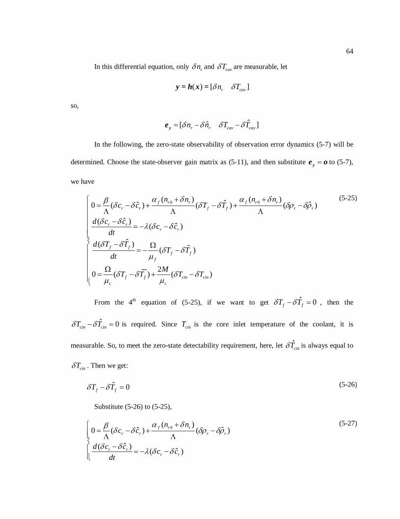
64
In this differential equation, only rnδ and cavTδ are measurable, let
( ) [ ]r cavn Tδ δy = h x =
so,
ˆˆ[ ]r r cav cavn n T Tδ δ δ δ= − −ye
In the following, the zero-state observability of observation error dynamics (5-7) will be
determined. Choose the state-observer gain matrix as (5-11), and then substitute =ye o to (5-7),
we have
0 0( ) ( )ˆ ˆˆ0 ( ) ( ) ( )
ˆ( ) ˆ( )
ˆ( ) ˆ( )
f r r f r rr r f f r r
r rr r
f ff f
f
n n n nc c T T
d c c c cdt
d T TT T
dt
α δ α δβ δ δ δ δ δρ δρ
δ δ λ δ δ
δ δδ δ
µ
+ += − + − + −
Λ Λ Λ−
= − −
− Ω= − −
2ˆˆ0 ( ) ( ) f f cin cinc c
MT T T Tδ δ δ δµ µ
Ω = − + −
(5-25)
From the 4th ˆ 0f fT Tδ δ− = equation of (5-25), if we want to get , then the
ˆ 0cin cinT Tδ δ− = is required. Since cinT is the core inlet temperature of the coolant, it is
measurable. So, to meet the zero-state detectability requirement, here, let cinTδ is always equal to
cinTδ . Then we get:
ˆ 0f fT Tδ δ− = (5-26)
Substitute (5-26) to (5-25),
0( )ˆˆ0 ( ) ( )
ˆ( ) ˆ( )
f r rr r r r
r rr r
n nc c
d c c c cdt
α δβ δ δ δρ δρ
δ δ λ δ δ
+= − + − Λ Λ
− = − −
(5-27)
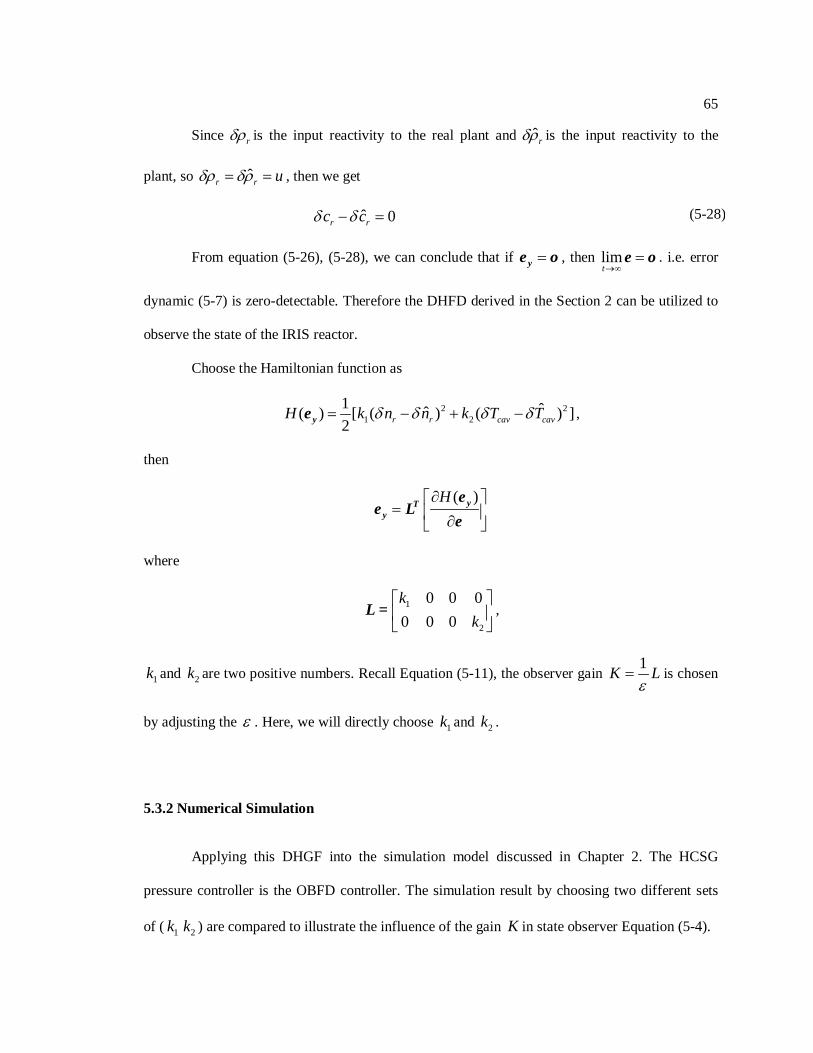
65
Since rδρ is the input reactivity to the real plant and ˆrδρ is the input reactivity to the
plant, so ˆr r uδρ δρ= = , then we get
ˆ 0r rc cδ δ− = (5-28)
From equation (5-26), (5-28), we can conclude that if =ye o , then limt→∞
=e o . i.e. error
dynamic (5-7) is zero-detectable. Therefore the DHFD derived in the Section 2 can be utilized to
observe the state of the IRIS reactor.
Choose the Hamiltonian function as
2 21 2
1 ˆˆ( ) [ ( ) ( ) ]2 r r cav cavH k n n k T Tδ δ δ δ= − + −ye ,
then
( )H∂ = ∂
yTy
ee L
e
where
1
2
0 0 00 0 0k
k
L = ,
1k and 2k are two positive numbers. Recall Equation (5-11), the observer gain 1K Lε
= is chosen
by adjusting the ε . Here, we will directly choose 1k and 2k .
5.3.2 Numerical Simulation
Applying this DHGF into the simulation model discussed in Chapter 2. The HCSG
pressure controller is the OBFD controller. The simulation result by choosing two different sets
of ( 1k 2k ) are compared to illustrate the influence of the gain K in state observer Equation (5-4).
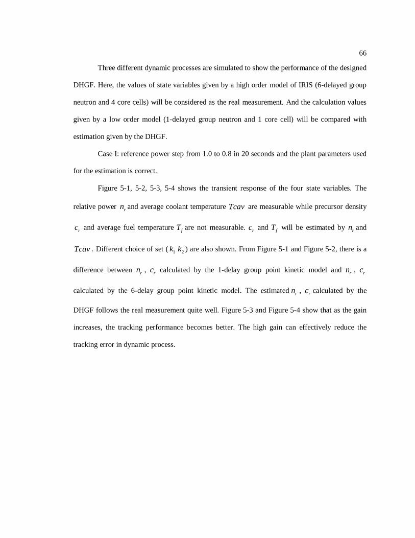
66
Three different dynamic processes are simulated to show the performance of the designed
DHGF. Here, the values of state variables given by a high order model of IRIS (6-delayed group
neutron and 4 core cells) will be considered as the real measurement. And the calculation values
given by a low order model (1-delayed group neutron and 1 core cell) will be compared with
estimation given by the DHGF.
Case I: reference power step from 1.0 to 0.8 in 20 seconds and the plant parameters used
for the estimation is correct.
Figure 5-1, 5-2, 5-3, 5-4 shows the transient response of the four state variables. The
relative power rn and average coolant temperature Tcav are measurable while precursor density
rc and average fuel temperature fT are not measurable. rc and fT will be estimated by rn and
Tcav . Different choice of set ( 1k 2k ) are also shown. From Figure 5-1 and Figure 5-2, there is a
difference between rn , rc calculated by the 1-delay group point kinetic model and rn , rc
calculated by the 6-delay group point kinetic model. The estimated rn , rc calculated by the
DHGF follows the real measurement quite well. Figure 5-3 and Figure 5-4 show that as the gain
increases, the tracking performance becomes better. The high gain can effectively reduce the
tracking error in dynamic process.
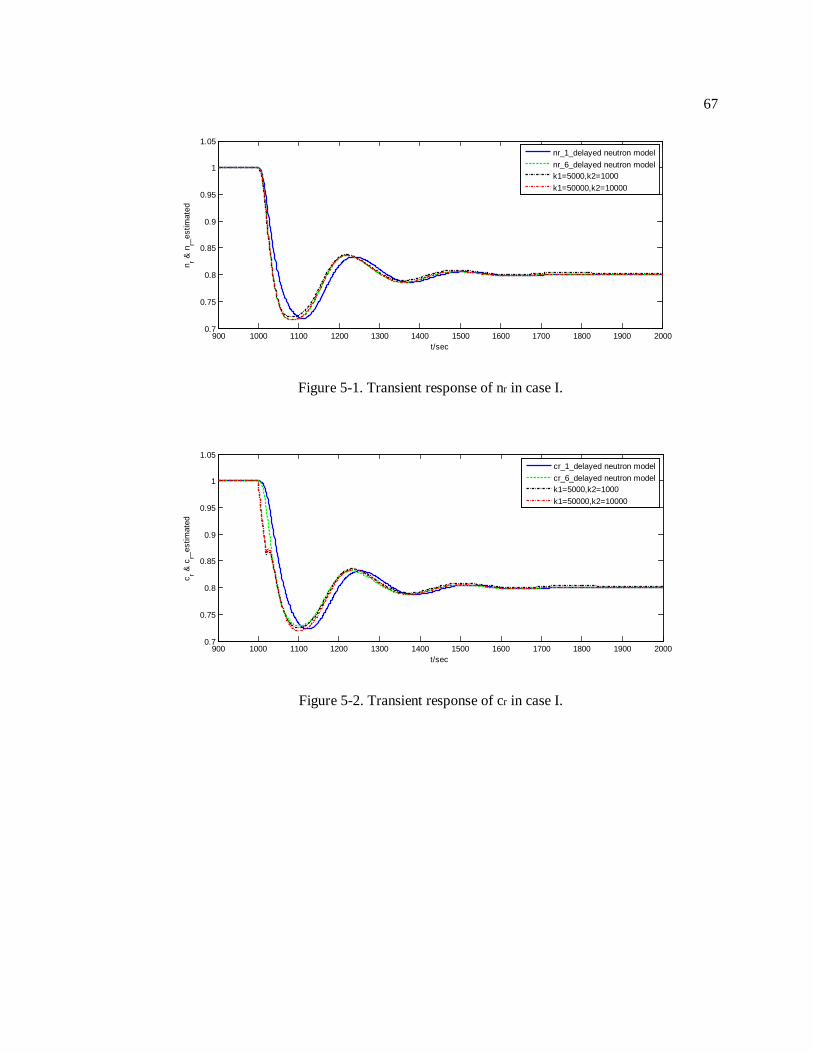
67
Figure 5-1. Transient response of nr in case I.
Figure 5-2. Transient response of cr in case I.
900 1000 1100 1200 1300 1400 1500 1600 1700 1800 1900 20000.7
0.75
0.8
0.85
0.9
0.95
1
1.05
t/sec
n r & n
r_est
imat
ed
nr_1_delayed neutron modelnr_6_delayed neutron modelk1=5000,k2=1000k1=50000,k2=10000
900 1000 1100 1200 1300 1400 1500 1600 1700 1800 1900 20000.7
0.75
0.8
0.85
0.9
0.95
1
1.05
t/sec
c r & c
r_est
imat
ed
cr_1_delayed neutron modelcr_6_delayed neutron modelk1=5000,k2=1000k1=50000,k2=10000
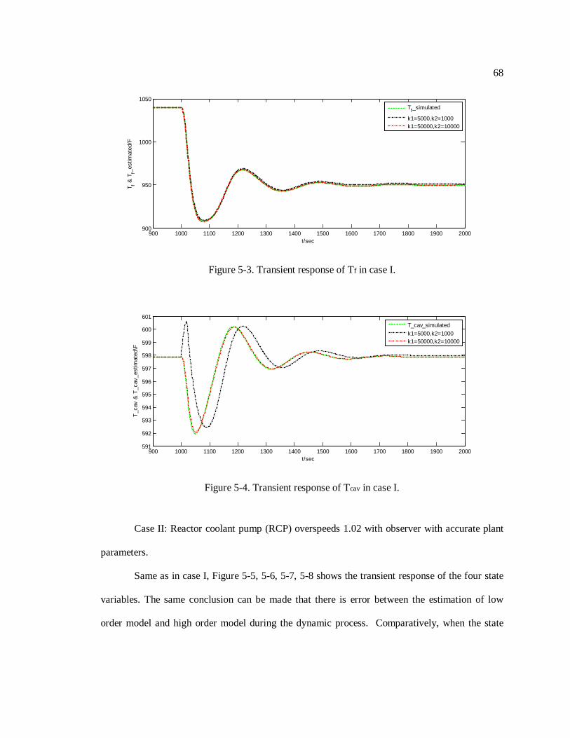
68
Figure 5-3. Transient response of Tf in case I.
Figure 5-4. Transient response of Tcav in case I.
Case II: Reactor coolant pump (RCP) overspeeds 1.02 with observer with accurate plant
parameters.
Same as in case I, Figure 5-5, 5-6, 5-7, 5-8 shows the transient response of the four state
variables. The same conclusion can be made that there is error between the estimation of low
order model and high order model during the dynamic process. Comparatively, when the state
900 1000 1100 1200 1300 1400 1500 1600 1700 1800 1900 2000900
950
1000
1050
t/sec
T f & T
f_est
imat
ed/F
Tf_simulated
k1=5000,k2=1000k1=50000,k2=10000
900 1000 1100 1200 1300 1400 1500 1600 1700 1800 1900 2000591
592
593
594
595
596
597
598
599
600
601
t/sec
T_ca
v &
T_c
av_e
stim
ated
\F
T_cav_simulatedk1=5000,k2=1000k1=50000,k2=10000

69
observer gain K is big enough, the DHGF can estimate the state valuables very well by using a
low order model.
Figure 5-5. Transient response of nr in case II.
Figure 5-6. Transient response of cr in case II.
900 1000 1100 1200 1300 1400 1500 1600 1700 1800 1900 20000.99
0.995
1
1.005
1.01
1.015
1.02
1.025
1.03
1.035
t/sec
n r & n
r_est
imat
ed
nr_1_delayed neutron modelnr_6_delayed neutron modelk1=5000,k2=1000k1=50000,k2=10000
900 1000 1100 1200 1300 1400 1500 1600 1700 1800 1900 20000.99
0.995
1
1.005
1.01
1.015
1.02
1.025
t/sec
c r & c
r_est
imat
ed
cr_1_delayed neutron modelcr_6_delayed neutron modelk1=5000,k2=1000k1=50000,k2=10000
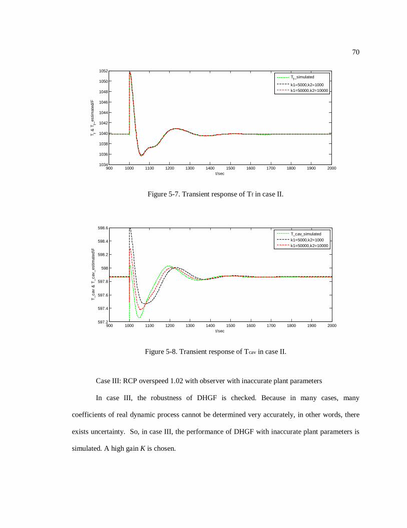
70
Figure 5-7. Transient response of Tf in case II.
Figure 5-8. Transient response of Tcav in case II.
Case III: RCP overspeed 1.02 with observer with inaccurate plant parameters
In case III, the robustness of DHGF is checked. Because in many cases, many
coefficients of real dynamic process cannot be determined very accurately, in other words, there
exists uncertainty. So, in case III, the performance of DHGF with inaccurate plant parameters is
simulated. A high gain K is chosen.
900 1000 1100 1200 1300 1400 1500 1600 1700 1800 1900 20001034
1036
1038
1040
1042
1044
1046
1048
1050
1052
t/sec
T f & T
f_est
imat
ed/F
Tf_simulated
k1=5000,k2=1000k1=50000,k2=10000
900 1000 1100 1200 1300 1400 1500 1600 1700 1800 1900 2000597.2
597.4
597.6
597.8
598
598.2
598.4
598.6
t/sec
T_ca
v &
T_c
av_e
stim
ated
\F
T_cav_simulatedk1=5000,k2=1000k1=50000,k2=10000

71
The following parameters are changed:
Table 5-1. Inaccurate parameters of DHGF for Simulation of Case III.
fµ cµ fα cα
Value used in Plant 0.4519 0.7357 -1.6500e-005 -4.0000e-004
Value used in Observer 0.5423 0.8828 -1.4850e-005 -3.6000e-004
Figures 5-9, 5-10, 5-11, 5-12 show the transient response of the four state variables. The
performance of DHGF is still good. While some parameters are changed, the low order model
results in a steady state error.
Figure 5-9. Transient response of nr in case III.
900 1000 1100 1200 1300 1400 1500 1600 1700 1800 1900 20000.995
1
1.005
1.01
1.015
t/sec
n r & n
r_est
imat
ed
nr_1_delayed neutron modelnr_6_delayed neutron modelk1=50000,k2=10000

72
Figure 5-10. Transient response of Cr in case III.
Figure 5-11. Transient response of Tf in case III.
900 1000 1100 1200 1300 1400 1500 1600 1700 1800 1900 20000.996
0.998
1
1.002
1.004
1.006
1.008
1.01
t/sec
c r & c
r_est
imat
ed
cr_1_delayed neutron modelcr_6_delayed neutron modelk1=50000,k2=10000
900 1000 1100 1200 1300 1400 1500 1600 1700 1800 1900 20001038
1039
1040
1041
1042
1043
1044
1045
1046
t/sec
T_f &
T_f
_est
imat
ed\F
T_f_simulated_lower_orderT_f_simulated_higher_orderk1=50000,k2=10000
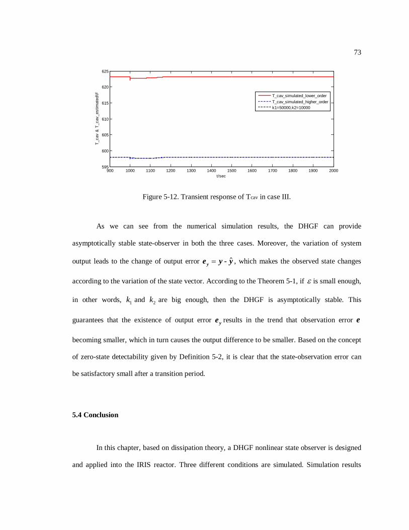
73
Figure 5-12. Transient response of Tcav in case III.
As we can see from the numerical simulation results, the DHGF can provide
asymptotically stable state-observer in both the three cases. Moreover, the variation of system
output leads to the change of output error ˆ=ye y - y , which makes the observed state changes
according to the variation of the state vector. According to the Theorem 5-1, if ε is small enough,
in other words, 1k and 2k are big enough, then the DHGF is asymptotically stable. This
guarantees that the existence of output error ye results in the trend that observation error e
becoming smaller, which in turn causes the output difference to be smaller. Based on the concept
of zero-state detectability given by Definition 5-2, it is clear that the state-observation error can
be satisfactory small after a transition period.
5.4 Conclusion
In this chapter, based on dissipation theory, a DHGF nonlinear state observer is designed
and applied into the IRIS reactor. Three different conditions are simulated. Simulation results
900 1000 1100 1200 1300 1400 1500 1600 1700 1800 1900 2000595
600
605
610
615
620
625
t/sec
T_ca
v &
T_c
av_e
stim
ated
\F
T_cav_simulated_lower_orderT_cav_simulated_higher_orderk1=50000,k2=10000

74
show that the performance of DHGF is better than a low order model which is used to estimate
state values. And when the observer gain K is chosen big enough, then the observer is
asymptotically stable and the estimated state values track the real state values well.
Chapter 6
Conclusion and Suggestion
6.1 Summary of Results
This thesis has demonstrated the design of a MIMO reliable LQG controller design for
IRIS power plant system. Then applying dissipation Hamiltonian theory, an observer-based
output feedback dissipation controller and a dissipation-based high gain filter are designed and
applied into the IRIS power plant.
Chapter 1 introduced the background and motivation of this thesis.
Chapter 2 presented the mathematical models of IRIS reactor core, helical-coil steam
generator and steam generator. These mathematical models are developed according to the
physical laws, i.e. neutron kinetics, heat transfer. Then, the mathematical model is implemented
in MATLAB/SIMULINK environment. This computer simulation model is used to determine the
dynamic response, the controller design and online state-observer design.
Chapter 3 introduces a detailed procedure to design a reliable LQG controller. The
reliable LQG controller is obtained by solving ARE and LMI. Then, the order of controller is
reduced to 9 by using Hankel norm approximation method. From the simulation result, the
reliable LQG controller can maintain the system stable when sensors drift in allowable range and
perform well in tracking reference signal.
Chapter 4 introduces dissipative Hamiltonian theory. Several basic definitions are given.
Then by referring the model used in level control of current U-tube steam generator, a nonlinear
observer-based feedback dissipation controller for the pressure control of HCSG is presented in

76
this chapter. The simulation results show that the OBFD can well stabilize the pressure of HCSG
and the OBFD controller can guarantee enough stable margins.
Chapter 5 introduces an online state-observer mechanism for the nonlinear reactor model.
First, since the dynamic model used to do the observer design should satisfy the zero-state
detectability and the simulation model cannot be used because it is complicated and does not
meet the requirement for the zero-state detectablity, a new and simple dynamic model used to the
observer design need to be derived. Then based on this model, applying the dissipation-based
high gain filter theorem, the state observer is designed. The simulation shows that the estimation
given by this state observer tracks the real value well.
6.2 Future Work
The following works are recommended for the future research.
1). The reliable LQG controller can maintain the system stable when sensors drift in
allowable range and perform well in tracking reference signal. However, compared with robust
control, for example, H∞ robust control, the reliable LQG does not perform well in the noise
rejection. So, the future work will focus on enhancing the ability to reject noise of reliable LQG
control.
2). For a complicated system, the observer matrix of the OBFD can only be obtained by
experience and validated by simulation. That is the limitation of the OBFD. So, how to choose an
effective matrix of the observer is recommended as the future research.
3). The DHGF is an effective state observer design method. The key step of this method
is to write the dynamic process in a model which satisfies the zero-state detectability. However, it
is not easy to realize this step, especially for a nonlinear and complicated dynamic process. How
to find an effective way to express the dynamic process which can be used to do the DHGF

77
design is recommended for the future work. Furthermore, Applying DHGF into the state
estimation of HCSG is recommended for future research since a nonlinear state space model is
given in Chapter 4.
78
Reference
[1]. J. W. HINES, “Advanced Instrumentation and Control Methods for Small and Medium
Reactors with IRIS Demonstration”, , Funding Opportunity Number: DE-PS07-07ID14812.
[2]. MARIO D. CARELLI, L. E. CONWAY, L. ORIANI, B. PETROVIC, C. V. LOMBARDI, M.
E. RICOTTI, A. C. O. BARROSO etc. “The Design and Safety Features of the IRIS Reactor,”
Nuclear Engineering and Design 230 (2004) 151-167
[3] M. D. Carelli et al., "The design and safety features of the IRIS reactor", Nuclear Engineering
and Design, 230 (2004), 151-167.
[4] G. D. Storrick and M. D. Carelli, "The IRIS (International Reactor Innovative and Secure)
and its Unique Advancement of the State-of the Art", Power and Energy Society General Meeting
- Conversion and Delivery of Electrical Energy in the 21st Century, 20-24 July 2008
[5] M. D. Carelli, "IRIS: A global approach to nuclear power renaissance", Nuclear News, pp. 32-
42, Sep. 2003
[6]. Shian-shing Shyu, “A Robust Multivariable Feedforward/Feedback Controller Design For
Integrated Power Control of Nuclear Power Plant”, PhD thesis, Pennsylvania State University,
May 2001, pp18-21.
[7]. IEEE committee report, "Dynamic models for steam and hydro turbines in power system
studies," IEEE Transactions on Power Apparatus and Systems, Vol.PAS-92, No.6, 1973,
pp.1904-1915.
[8]. P. Kundur, “Power system stability and control”, New York: McGraw-Hill.
[9]. Wiktor Bolek, Jerzy Sasiadek, Tadeusz Wisniewski, “Two-valve control of a large steam
turbine”, Control Engineering Practice, 10(2002), pp.365-377.
[10]. Alexander Leyzerovich, “Large Power Steam Turbines”, Design Volume 1, PennWell
Publishing Company, Tulsa, Oklahoma, pp.218
79
[11]. http://www.mathworks.com/support/tech-notes/1600/1605.html#intro
[12]. A. Ray and S. Phoha, “Calibration and estimation of redundant signals for real-time
monitoring and control”, Signal Process, 83, pp. 2593-2605 (2003).
[13]. H. M. Hashwmian, Maintenance of Process Instrumentation in Nuclear Power Plant, p.29,
Springer, New York (2006)
[14]. Huai-Ni Wu, “Reliable LQ fuzzy control for continuous-time nonlinear systems with
actuator faults,” IEEE Transaction on System, Man, and Cybernetics-part B: Cybernetics, Vol.
34, No. 4, August 2004
[15]. Robert J. Veillette, “Reliable linear-quadratic state-feedback control”, Automatic, Vol. 31,
No. 1, pp137-143, 1995
[16]. Li Yu, “An LMI approach to reliable guaranteed cost control of discrete-time systems with
actuator failure”, Applied Mathematics and Computation 162(2005) 1325-1331
[17]. Dengfeng Zhang, Hongyu Su, et. “LMI approach to reliable guaranteed cost control with
multiple criteria constraints: The actuator faults case”, Int. J. Robust Nonlinear Control 2009; 19:
884-899
[18]. G. H. Yang, J. Lam, and J. L. Wang, “Reliable H∞
[19]. Y. W. Liang, D. C. Liaw, and T. C. Lee, “Reliable control of nonlinear systems,” IEEE
Trans. Automat. Contr. Vol. 45, No. 4, pp. 706-710, 2000
Control for affine nonlinear systems,”
IEEE Trans. Automat. Contr. Vol, 43, pp. 1112-1117, Aug. 1998
[20]. G.H. Yang, J.L. Wang and Y.C. Soh, “Reliable LQG control with sensor failures”, IEEE
Proc. Control Theory Application. Vol. 147, No. 4, July 2000
[21]. Yin Guo, Robert M. Edwards, “Reliable LQG Controller Design with Sensor Failure for
Nuclear Power Plant with IRIS Demonstration”, Tran. of ANS 2009 Winter Meeting, Washington,
DC, Nov 2009
80
[22]. X. Jin, R. M. Edwards and A. Ray, “Integrated Robust and Resilient Control for Nuclear
Power Plants,” Proc. of Sixth ANS International Topical Meeting on NPIC & HMIT, Knoxville,
TN, Apr 2009
[23]. M. V. KOTHARE, B. METTLER, M. MORARI, P. BENDOTTI, and C. -M. FALINOWER,
“Level Control in the Steam Generator of A Nuclear Power Plant,” IEEE Trans. Control Syst.
Technol., vol. 8, no. 1, pp. 55-69, 2000.
[24]. M. G. NA, “Auto-tuned PID Controller Using A Model Predictive Control Method for the
Steam Generator Water Level,” IEEE. Trans. Nucl. Sci, vol.48, no. 5, pp. 1664-1671, Oct, 2001.
[25]. B. H. CHO, H. C. NO, “Design of Stability-guaranteed Fuzzy Logic Controller for Nuclear
Steam Generators,” IEEE Trans. Nucl. Sci., vol. 43, no. 2, pp. 716-730, Apr. 1996.
[26]. S. R. MUNASINGHE, M.-S. KIM, and J. –J. LEE, “Adaptive Neurofuzzy Controllerto
Regulate UTSG Water Level in Nuclear Plants,” IEEE Trans. Nucl. Sci., vol. 52, no. 1, pp. 421-
429, Feb. 2005
[27]. YANHONG LIU, JIANYONG LI and CHUNWEN LI, “Dissipative Hamiltonian
Realization of Multi-machine Multi-load Power System,” 16th
[28]. YUZHEN WANG, DAIZHAN CHEN, CHUNWEN LI and YOU GE, “Dissipative
Hamiltonian Realization and Energy-Based L
IEEE International Conference on
Control Applications Part of IEEE Multi-conference on system and control, Singapore, Oct. 1-3,
2007
2
[29]. J. DE LEON-MORALES, G. ESPINOSA-PEREZ, I. MACIAS-CARDOSO, “Observer-
based Control of A Synchronous Generator: A Hamiltonian Approach,” Electrical Power and
Energy Systems 24 (2002) 655-663
-Disturbance Attenuation Control of Multimachine
Power Systems,” IEEE Transaction on Automatic Control, Vol. 48, No. 8, Aug 2003
81
[30]. ZHE DONG, XIAOJIN HUANG and JUNTING FENG, “Nonlinear Observer-based
Feedback Dissipation Load-following Control for Nuclear Reactors,” IEEE Transactions on
nuclear science, vol. 56 no. 1 Feb. 2009
[31]. D. CHENG, S. SPURGEON, and J. XIANG, “On the Development of Generalized
Hamiltonian Realization,” Proc. IEEE Conf. Decision and Control, Sydney, Australia, 2000, vol.5,
pp. 5125-5130
[32]. Z. XI, G. FENG, D. CHENG, and Q. LU, “Nonlinear Decentralized Saturated Controller
Design for Power System,” IEEE Trans. Control Syst. Technol., Vol. 11, no. 4, pp 539-547, 2003
[33]. ZHE DONG, XIAOJIN HUANG and JUNTING FENG, “Water-Level Control for the U-
Tube Steam Generator of Nuclear Power Plants Based on Output Feedback Dissipation”, IEEE
Transaction on Nuclear Science, Vol. 56. No. 3, June. pp 1600-1612.
[34]. M. A. SCHULTZ, Control of Nuclear Reactor and Power Plants, 2nd
[35]. J. W. HINES, J. M. DOSTER, R. M. EDWARDS and B. R. UPADHYAYA etc, “Advanced
Instrumentation and Control Methods for Small and Medium Reactors with IRIS Demonstration”,
Annual Report 2008, Report No. DE-FG07-07ID14895/UTNE/2008-4.
ed. McGraw-Hill,
New York, 1961.
[36]. F. P. RAMALHO, “Nonlinear H∞
[37]. M. V. KOTHARE, BERNARD METTLER, and MANFRED MORARI etc., “Level Control
in the Steam Generator of a Nuclear Power Plant”, IEEE Transaction on Control System
Technology, Vol. 8. No. 1, Jan. pp 55-69, 2000.
Control of Nuclear Steam Generators”, Ph.D. Dissertation,
University of Michigan, Ann Arbor, Michigan, USA, 2002
[38]. B. D. O. Anderson and J. B. Moore, optimal Filtering. Englewood Cliffs, N. J.; Prentice,
1979.
[39]. J. L. Tylee, “On-line failure detection in nuclear power plant instrumentation”, IEEE
Transaction. Automation Control, Vol 28, no.3 pp 406-415, 1983.
82
[40]. D. Y. Oh and H. C. No, “Instrumentation failure detection and reconstruction methodology
in space-time nuclear reactor dynamic systems with fixed in-core detectors,” IEEE Transaction
Nuclear Science, vol. 38, no. 5, pp 1026-1034, Oct. 1991
[41].K.Roy, R. N. Banavar and S. Thangasamy, “Application of fault detection and identification
(FDI) techniques in power regulating systems of nuclear reactors,” IEEE Transaction Nuclear
Science, vol. 45, no. 6 pp. 3184-3201, Dec 1998.
[42]. Krener AJ, Isidori A, “Linearization by output injection and nonlinear observers,” System
and Control Letters 1983; 3:47-52
[43]. Bestle D, Zeitz M. “Canonical form observer design for nonlinear time-variable systems,”
International Journal of Control 1983; 38:419-431
[44]. Xia XH, Gao WB. “Nonlinear observer design by observer error linearization,” SIAM
Journal on Control and Optimization 1989; 27:199-216
[45]. Keller H. “Nonlinear observer design by transformation into a generalized observer
canonical form,” International Journal of Control 1987; 46:1915-1930
[46]. Rudolph J, Zeitz M. “A block triangular nonlinear observer normal norm,” System and
control letters 1994; 23:1-8
[47]. Saberi A, Sannuti P. “Observer design for loop transfer recovery and for uncertain dynamic
systems,” IEEE transaction on Automatic Control, 1990; 35:878-897
[48]. Saberi A, Chen BM, Sannuti P. Loop Transfer Recovery: Analysis and Design, Spring:
Berlin 1993.
[49]. Gauthier JP, Hammouri H, Othman S. A simple observer for nonlinear systems application
to bioreactors. IEEE Transactions on Automatic Control 1992; 37: 875-880.
[50]. Dong Z, Feng J. Huang X, Zhang L. Dissipation-based high gain filter for monitoring
nuclear reactors. IEEE Transactions on Nuclear Science. Vol 57, No 1, Feb 2010.

83
[51]. Jian Zhang, Gang Feng and Hongbing Xu, “Observer design for nonlinear discrete-time
systems: Immersion and dynamic observer error linearization techniques,” Int. J. Robust
Nonlinear Control 2010; 20: 504-514.
[52]. A. J. Van Der Schaft, L2
[53]. http://www.mathworks.com/products/simulink/
-gain and passivity techniques in nonlinear control, Berlin,
Germany: Springer, 1999.

84
Appendix A
A
Nomenclatures For OBFD Nonlinear State Space Model
Flow area of subcooled region sc
A Cross section of boiling region b
A Flow area of super heated region s
H Total enthalpy of water in the subcooled region d
h Enthalpy of liquid water in the subcooled region d
h Enthalpy of liquid water in the boiling region f
h Enthalpy of steam in the boiling region g
h Latent heat of vaporization fg
h Enthalpy of feedwater fw
h Average enthalpy of the two-phase flow in the boiling region b
h Enthalpy of the steam in the super heated region s
L Length of subcooled region sc
L Length of boiling region b
L Length of super heated region s
L Length of tube total
M Mass of the water in the subcooled region sc
M Mass of the water in the boiling region b
M Mass of the water in the super heated region s
P Pressure of steam in the super heated region sc
P Pressure of saturated steam sat
P Pressure of the water in the sub cooled region b
Q Heat transferred from metal wall to the second side in the subcooled region sc
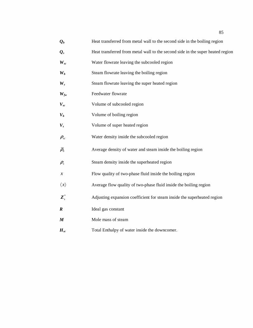
85
Q Heat transferred from metal wall to the second side in the boiling region b
Q Heat transferred from metal wall to the second side in the super heated region s
W Water flowrate leaving the subcooled region sc
W Steam flowrate leaving the boiling region b
W Steam flowrate leaving the super heated region s
W Feedwater flowrate fw
V Volume of subcooled region sc
V Volume of boiling region b
V Volume of super heated region s
scρ Water density inside the subcooled region
bρ Average density of water and steam inside the boiling region
sρ Steam density inside the superheated region
x Flow quality of two-phase fluid inside the boiling region
x⟨ ⟩ Average flow quality of two-phase fluid inside the boiling region
*sZ Adjusting expansion coefficient for steam inside the superheated region
R Ideal gas constant
M Mole mass of steam
H Total Enthalpy of water inside the downcomer. sc
86
Appendix B
%model_reduction_new
Reliable LQG MATLAB Code
clear all clc load ABCD A=Ar; B=Br; C=Cr; D=Dr n=rank(A); I2=eye(2); V1=1e4*eye(n); V1=1000*eye(n); %V1=B*B'; %R1=V1; %R1=0.1*eye(n); R1=0.01*eye(n); V2=0.99*I2; R2=diag([0.1 10]); R2=diag([0.001 1]) %R2=diag([0.1 100]); %R2=diag([10 1]); %R2=diag([0.5 1]); alpha0=diag([1 0.5]); %alpha0=diag([1 1]); beta=diag([0 1]); %beta=diag([0 0.5]); R0=diag([1 0.021]); %R0=diag([1 1]); disp('eig(inv(V2)-R0*beta)=') eig(inv(V2)-R0*beta) pause temp0=C'*inv((I2-beta^2)*V2+inv(R0)*beta)*(I2-beta^2)*C; Q=are(A',temp0,V1); eig(Q)

87
eig(A'-temp0*Q) disp('eigenvalue of ATrans-temp0*Q') pause %Step 3 E1inf=(I2-beta^0.5*R0^0.5*V2*beta^0.5*R0^0.5)^(-0.5)*beta^0.5*R0^0.5*C; V0=inv(inv(V2)-beta*R0); Cbar=(I2+V0*beta*R0)*C; A0=A+Q*E1inf'*E1inf; B10=Q*Cbar'*(V0+beta*inv(R0))^(-0.5); temp1=[R1^0.5;zeros(2,n)]; temp2=[zeros(n,2);R2^0.5]; %Solve LMI setlmis([]); X0=lmivar(1,[n+2 1]); X1=lmivar(1,[n 1]); W=lmivar(2,[2 n]); lmiterm([-1 1 1 X1],1,1); % LMI #1: X1 lmiterm([-2 1 1 X0],1,1); % LMI #2: X0 lmiterm([1 1 1 X1],A0,1,'s'); % LMI #1: A0*X1+X1*A0' lmiterm([1 1 1 W],B,1,'s'); % LMI #1: B*W+W'*B' lmiterm([1 1 1 0],B10*B10'); % LMI #1: B10*B10' lmiterm([1 2 1 X1],E1inf,1); % LMI #1: E1inf*X1 lmiterm([1 2 2 0],-I2); % LMI #1: -I2 lmiterm([2 1 1 X0],1,-1); % LMI #2: -X0 lmiterm([2 2 1 X1],1,temp1'); % LMI #2: X1*temp1' lmiterm([2 2 1 -W],1,temp2'); % LMI #2: W'*temp2' lmiterm([2 2 2 X1],1,-1); % LMI #2: -X1 IRIS_LMI=getlmis; %c=mat2dec(IRIS_LMI,eye(n+1)); c=mat2dec(IRIS_LMI,eye(n+2),zeros(n,n),zeros(2,n)); options=[1e-5,0,0,0,0]; [copt,xopt]=mincx(IRIS_LMI,c,options); X0opt=dec2mat(IRIS_LMI,xopt, X0); X1opt=dec2mat(IRIS_LMI,xopt, X1); Wopt=dec2mat(IRIS_LMI,xopt, W); Jmax=trace(X0opt)+trace(R1*Q); G=Q*C'*inv((I2-beta^2)*V2+inv(R0)*beta)*inv(alpha0); K=Wopt*inv(X1opt) F=A0-G*alpha0*inv(I2-V2*beta*R0)*C+B*K;
88
Ggcc=G; Kgcc=K; Fgcc=F; save('FGK','G','K','F'); for i=0:0.1:1 alpha=diag([1 i]); Ae=[A B*K;G*alpha*C F]; Be=[D] disp('Eigenvalue of Ae') eig(Ae) end