Reliable Attribute-Based Object Recognition Using High …yezhouyang.engineering.asu.edu/wp-content/uploads/2016/08/ECCV20… · Reliable Attribute-Based Object Recognition 3 (a)

Reliable Attribute-Based Object RecognitionUsing High Predictive Value Classifiers

Wentao Luan1, Yezhou Yang2, Cornelia Fermuller2, John S. Baras1

1 Institute for Systems Research, University of Maryland, College Park, USA2 Computer Vision Lab, University of Maryland, College Park, USA

[email protected], [email protected], [email protected], [email protected]

Abstract. We consider the problem of object recognition in 3D usingan ensemble of attribute-based classifiers. We propose two new conceptsto improve classification in practical situations, and show their imple-mentation in an approach implemented for recognition from point-clouddata. First, the viewing conditions can have a strong influence on classi-fication performance. We study the impact of the distance between thecamera and the object and propose an approach to fusing multiple at-tribute classifiers, which incorporates distance into the decision making.Second, lack of representative training samples often makes it difficultto learn the optimal threshold value for best positive and negative de-tection rate. We address this issue, by setting in our attribute classifiersinstead of just one threshold value, two threshold values to distinguisha positive, a negative and an uncertainty class, and we prove the theo-retical correctness of this approach. Empirical studies demonstrate theeffectiveness and feasibility of the proposed concepts.

1 Introduction

Reliable object recognition from 3D data is a fundamental task for active agentsand a prerequisite for many cognitive robotic applications, such as assistiverobotics or smart manufacturing. The viewing conditions, such as the distance ofthe sensor to the object, the illumination, and the viewing angle, have a stronginfluence on the accuracy of estimating simple as well as complex features, andthus on the accuracy of the classifiers. A common approach to tackle the prob-lem of robust recognition is to employ attribute based classifiers, and combinethe individual attribute estimates by fusing their information [1],[2],[3].

This work introduces two concepts to robustify the recognition by addressingcommon issues in the processing of 3D data, namely the problem of classifierdependence on viewing conditions, and the problem of insufficient training data.

We first study the influence of distance between the camera and the object onthe performance of attribute classifiers. Unlike 2D image processing techniques,which usually scale the image to address the impact of distance, depth basedobject recognition procedures using input from 3D cameras tend to be affectedby distance-dependent noise, and this effect cannot easily be overcome [4].

2 W. Luan, Y. Yang, C. Fermuller, J. S. Baras

We propose an approach that addresses effects of distance on object recog-nition. It considers the response of individual attribute classifiers’ depending ondistance and incorporates it into the decision making. Though, the main fac-tor studied here is distance, our mathematical approach is general, and can beapplied to handle other factors affected by viewing conditions, such as lighting,viewing angle, motion blur, etc.

To implement the attribute classifiers, usually, the standard threshold methodis used to determine the boundary between positive and negative examples. Us-ing this threshold the existence of binary attributes is determined, which in turncontrols the overall attribute space. However, there may not be enough train-ing samples to accurately represent the underlying distributions, which makes itmore difficult to learn one good classification threshold that minimizes the num-ber of incorrect predictions (or maximizes the number of correct predictions).

Here we present an alternative approach which applies two thresholds withone aiming for a positive predictive value (PPV), giving high precision for posi-tive classes, and the other aiming for a negative predictive value (NPV), givinghigh precision for negative classes. Each classifier can then have three types ofoutput: “positive” when above the high PPV threshold, “negative” when belowthe high NPV threshold and “uncertain” when falling into the interval betweenthe two thresholds. Recognition decisions, when fusing the classifiers, are thenmade based on the positive and negative results. More observations thereby areneeded for drawing a conclusion, but we consider this trade-off affordable, sincewe assume that our active agent can control the number of observations. Notethat two threshold approaches have previously been used for the purpose ofachieving results of high confidence, for example in [5], and in probability ratiotests.

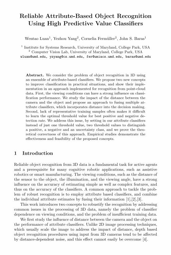
The underlying intuition here is that it should be easier to obtain the highPPV and NPV thresholds than the classical Bayes threshold (minimizing theclassification error), when the number of training samples is too small to repre-sent well the underlying distribution. Fig. 1a illustrates the intuition. The topfigure shows the ground truth distributions (of the classification score) of thepositive and negative class. The lower figure depicts the estimated distributionsfrom training samples, which are biased due to an insufficient amount of data.Furthermore, as our experiment revealed, even the ground truth distributioncould be dependent on viewing conditions, which makes it more challenging tolearn a single optimal threshold. In such a case, the system may end up withan inaccurate Bayes threshold. However, it is still possible to select high PPV(NPV) thresholds by setting these thresholds (at a safe distance) away from thenegative (positive) distribution.

For each basic (attribute) classifier, we can also define a reliable workingregion indicating a fair separation of the distributions of positive and negativeclasses. Hence our approach can actively select “safe” samples and discard “un-safe” ones in unreliable regions. We prove the asymptotic correctness of thisapproach in section 3.3.

Reliable Attribute-Based Object Recognition 3

(a) (b)

Fig. 1. (a): Illustration of common conditional probability density functions of thepositive and negative class. Top: ground truth distribution of the two classes; bottom:a possible distribution represented by the training data. Blue line: positive class; redline: negative class. dashed line: (estimated) Bayes threshold; solid line: high PPV andNPV thresholds. (b): The relationship of Objects (O), attributes (Fi), environmentalvariables (Ek) and observations (Zk

i ) in our model.

Integrating both concepts, our complete approach to 3D object recognitionworks as follows: Offline we learn attribute classifiers, which are distance depen-dent. In practice, we discretize the space into n distance intervals, and for eachinterval we learn classifiers with two thresholds. Also, we decide for each at-tribute classifier a reliable range of distance intervals. During the online processour active system takes RGBD images as it moves around the space. For eachinput image, it first decides the distance interval in order to use the classifierstuned to that interval. Classifier measurements from multiple images are thencombined via maximum a posteriori probability (MAP) estimation.

Our work has three main contributions: 1) We put forward a practical frame-work for fusing component classifiers’ results by taking into account the distance,to accomplish reliable object recognition. 2) We prove our fusion framework’sasymptotic correctness under certain assumptions on the attribute classifier andsufficient randomness of the input data. 3) The benefits of introducing simpleattributes, which are more robust to viewing conditions, but less discriminative,are demonstrated in the experiment.

2 Related Work

Creating practical object recognition systems that can work reliably under dif-ferent viewing conditions, including varying distance, viewing angle, illuminationand occlusions, is still a challenging problem in Computer Vision. Current sin-gle source based recognition methods have robustness to some extent: featureslike SIFT [6] or the multifractal spectrum vector (MFS) [7] in practice are in-variant to a certain degree to deformations of the scene and viewpoint changes;geometric-based matching algorithms like BOR3D [8] and LINEMOD [9] canrecognize objects under large changes in illumination, where color based algo-


rithms tend to fail. But in complicated working environments, these systemshave difficulties to achieve robust performance.

One way to deal with variations in viewing conditions is to incorporate dif-ferent sources of information (or cues) into the recognition process. However,how to fuse the information from multiple sources, is still an open problem.

Early fusion methods have tried to build more descriptive features by com-bining features from sources like texture, color and depth before classification.For example, Asako et al. builds voxelized shape and color histogram descrip-tors [1] and classifies objects using SVM, while in [10] information from color,depth, SIFT and shape distributions is described by histograms and objects arerecognized using K-Nearest Neighbors.

Besides early fusion, late fusion also has gained much attention and achievesgood results. Lutz at al. [3] proposes a probabilistic fusion approach, calledMOPED [11], to combine a 3D model matcher, color histograms and featurebased detection algorithm, where a quality factor, representing each method’sdiscriminative capability, is integrated in the final classification score. Meta in-formation [12] can also be added to create a new feature. Ziang et al. [2] blendsclassification scores from SIFT, shape, and color models with meta features pro-viding information about each model’s fitness from the input scene, which resultsin high precision and recall on the Challenge and Willow datasets. Consideringinfluences due to viewing conditions, Ahmed [13] applies an AND/OR graphrepresentation of different features and updates a Bayes conditional probabilitytable based on measurements of the environment, such as intensity, distance andocclusions. However, these methods may suffer from inaccurate estimation of theconditional probabilities involved, because of insufficient training data.

In our work, we propose a framework for object recognition using multipleattribute classifiers, which considers both, effects due to viewing conditions andeffects due to biased training data that systems face in practice. We implementour approach for an active agent that takes advantage of multiple inputs atvarious distances.

3 Assumptions and Formulation

Before going into the details and introducing the notation, let us summarizethis section. Section 3.1 defines the data fusion of the different classificationresults through MAP estimation. Section 3.2 proves that MAP estimation willclassify correctly under certain requirements and assumptions. The requirementsare restrictions on the values of the PPV and NPV. The assumptions are thatour attribute classifiers perform correctly in the following sense: A ground truthpositive value should be classified as positive or uncertain and a ground truthnegative value should be classified as negative or uncertain. Finally section 3.3proves asymptotic correctness of MAP estimation. The estimation will converge,even if the classifiers don’t perform correctly, under stronger requirements on thevalues of the PPV and NPV.


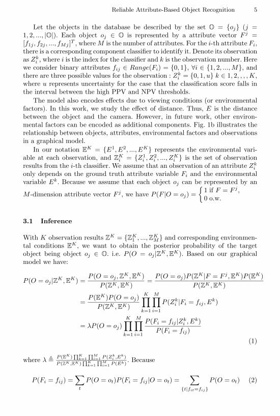
Let the objects in the database be described by the set O = {oj} (j =1, 2, ..., |O|). Each object oj ∈ O is represented by a attribute vector F j =[f1j , f2j , ..., fMj ]

T , whereM is the number of attributes. For the i-th attribute Fi,there is a corresponding component classifier to identify it. Denote its observationas Zki , where i is the index for the classifier and k is the observation number. Herewe consider binary attributes fij ∈ Range(Fi) = {0, 1}, ∀i ∈ {1, 2, ...,M}, andthere are three possible values for the observation : Zki = {0, 1, u} k ∈ 1, 2, , , ,K,where u represents uncertainty for the case that the classification score falls inthe interval between the high PPV and NPV thresholds.

The model also encodes effects due to viewing conditions (or environmentalfactors). In this work, we study the effect of distance. Thus, E is the distancebetween the object and the camera. However, in future work, other environ-mental factors can be encoded as additional components. Fig. 1b illustrates therelationship between objects, attributes, environmental factors and observationsin a graphical model.

In our notation EK = {E1, E2, ..., EK} represents the environmental vari-able at each observation, and ZKi = {Z1

i , Z2i , ..., Z

Ki } is the set of observation

results from the i-th classifier. We assume that an observation of an attribute Zkionly depends on the ground truth attribute variable Fi and the environmentalvariable Ek. Because we assume that each object oj can be represented by an

M -dimension attribute vector F j , we have P (F |O = oj) =

{1 if F = F j ,0 o.w.

3.1 Inference

With K observation results ZK = {ZK1 , ...,ZKM} and corresponding environmen-tal conditions EK , we want to obtain the posterior probability of the targetobject being object oj ∈ O. i.e. P (O = oj |ZK ,EK). Based on our graphicalmodel we have:

P (O = oj |ZK ,EK) =P (O = oj ,ZK ,EK)

P (ZK ,EK)=P (O = oj)P (ZK |F = F j ,EK)P (EK)

P (ZK ,EK)

=P (EK)P (O = oj)

P (ZK ,EK)

K∏k=1

M∏i=1

P (Zki |Fi = fij , Ek)

= λP (O = oj)

K∏k=1

M∏i=1

P (Fi = fij |Zki , Ek)

P (Fi = fij)

(1)

where λ , P (EK)∏Kk=1

∏Mi=1 P (Zki ,E

k)

P (ZK ,EK)∏Kk=1

∏Mi=1 P (Ek)

. Because

P (Fi = fij) =∑t

P (O = ot)P (Fi = fij |O = ot) =∑

{t|fit=fij}

P (O = ot) (2)


Finally, we have

P (O = oj |ZK ,EK) = λP (O = oj)

K∏k=1

M∏i=1

P (Fi = fij |Zki , Ek)∑{t|fit=fij} P (O = ot)

. (3)

The recognition A then is derived using MAP estimation as:

A , argmaxoj

P (O = oj |ZK ,EK). (4)

In our framework, we use the high positive and negative predictive value obser-vations (Z = 0, 1) to determine the posterior probability.

We also take into account the influence of environmental factors. That is,only observations from a reliable working region are adopted in the probabil-ity calculation. When the environmental factor is distance, the reliable workingregion is defined as a range of depth values where the attribute classifier workreasonably well. We treat a range of distance values as a reliable working re-gion for a classifier, if the detection rate for this range is larger than a certainthreshold, and the PPV meets the system requirement.

This requirement for the component classifiers is achievable if the positiveconditional probability density function of the classification score has a non-overlapping area with the negative one. Then we can tune the classifier’s PPVthreshold towards the positive direction (towards left in Fig. 1a) to achieve ahigh precision with a guarantee of minimum detection rate.

Formally speaking, our P (Fi = fij |Zki , Ek) is defined as:

P (Fi = 1|Zki , Ek) =

p+i if ek ∈ Ri & zki = 1,1− p−i if ek ∈ Ri & zki = 0,∑t|fit=fij P (O = ot) o.w.

(5)

where Ri is the set of environmental values for which the i-th classifier canachieve a PPV p+i with a detection rate lower bound. As before, k denotes thek-th observation. If the above condition is not met, either the recognition isdone in an unreliable region or the answer is uncertain. Now equation (3) canbe rewritten as:

P (O = oj |ZK ,EK) = λP (O = oj)

K∏k=1

∏i∈Ik

P (Fi = fij |Zki , Ek)∑{t|fit=fij} P (O = ot)

, (6)

where Ik = Ik+ ∪ Ik− is the index set of recognized attributes at the k-th obser-vation with Ik+ = {i|ek ∈ Ri & zki = 1} and Ik− = {i|ek ∈ Ri & zki = 0}.

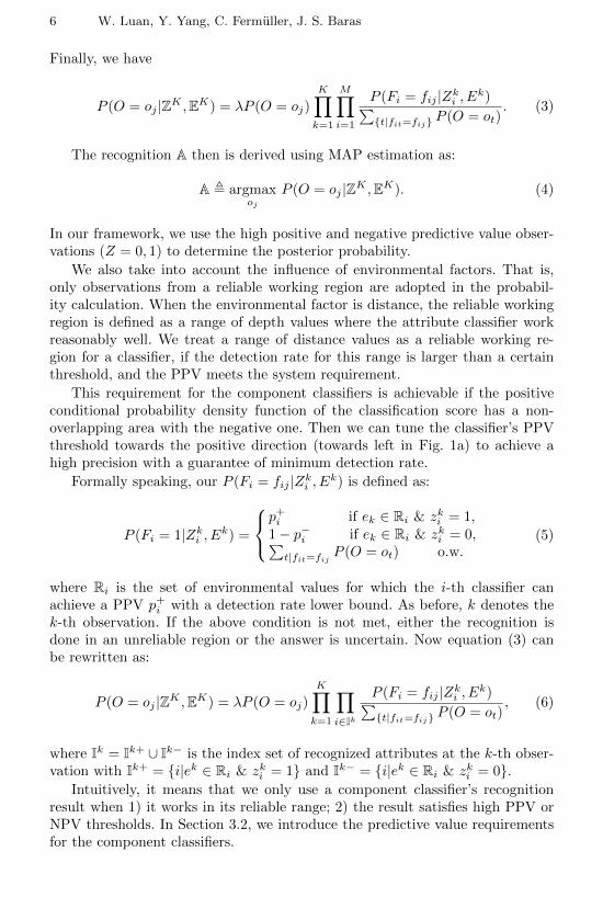
Intuitively, it means that we only use a component classifier’s recognitionresult when 1) it works in its reliable range; 2) the result satisfies high PPV orNPV thresholds. In Section 3.2, we introduce the predictive value requirementsfor the component classifiers.


3.2 System Requirement for the Predictive Value

Here we put forward a predictive value requirement for each component classifierto have correct MAP estimations assuming there do not exist false positives orfalse negatives from observations.

To simplify our notation, we define the prior probability of object πj ,P (O = oj), j = (1, 2, ..., No) and the prior probability of attribute Fi being

positive as wi ,∑{t|fit=1}

πt, (i = 1, 2, ...,M). For each attribute, the following

ratios are calculated: r+i , max(1,max{t|fit=0} πtmin{t|fit=1} πt

), r−i , max(1,max{t|fit=1} πtmin{t|fit=0} πt

).

I+Fj and I−Fj are the index sets of positive and negative attributes in F j , andthe reliably recognized attributes’ indexes at the k-th observation are denotedas I = {I1, I2, ..., IK} (Ik as defined in section 3.1). We next state the conditionsfor correct MAP estimation.

Theorem 1. If the currently recognized attributes⋃k Ik can uniquely identify

object oj, i.e.⋃k Ik+ ⊆ IF+

j,⋃k Ik− ⊆ IF−j , ∀t 6= j,

⋃k Ik+ * IF+

tor⋃k Ik− *

IF−t , and if ∀i ∈ {1, 2, ...,M} the classifiers’ predictive values satisfy p+i ≥r+i wi

1+(ri−1)wi and p−i ≥r−i (1−wi)

wi+r−i (1−wi)

, then the MAP estimation result A = {oj}.

This requirement means that if 1) the attributes can differentiate an objectfrom others, and 2) the component classifiers’ predictive values satisfy the re-quirement, then for the correct observation input, the system is guaranteed tohave a correct recognition result.

Proof. Based on (6) and the definition above, the posterior probability of oj is,

P (O = oj |ZK ,EK) = λπj

K∏k=1

( ∏i∈Ik+

p+iwi

∏i∈Ik−

p−i1− wi

). (7)

Because the current observed attributes⋃k Ik can uniquely identify oj , we

will have ∀og ∈ O/{oj}, ∃Ig ⊆⋃k Ik and Ig 6= ∅, s.t. ∀i ∈ Ig, fgi = 0 if i ∈ Ik+

or fgi = 1 if i ∈ Ik−. Thus, ∀og ∈ O/{oj},

P (O = og|ZK ,EK) = λπg

K∏k=1

( ∏i∈Ik+/Ig

p+iwi

∏i∈Ik+

⋂Ig

1− p+i1− wi∏

i∈Ik−/Ig

p−i1− wi

∏i∈Ik−

⋂Ig

1− p−iwi

).

(8)

Since for each classifier, p+i ≥r+i wi

1+(r+i −1)wiand r+i = max(1,

max{t|fit=0} πtmin{t|fit=1} πt

),

we have πjp+iwi≥ πg

1−p+i1−wj and

p+iwi≥ 1 ≥ 1−p+i

1−wi . For similar reasons, we have

πjp−i

1−wi ≥ πg1−p−iwj

andp−i

1−wi ≥ 1 ≥ 1−p−iwi

. Also since Ig 6= ∅, we can have (7) >

(8), an thus the conclusion is reached.


From the proof, we can extend the result to a more general case: if thecurrently recognized attributes cannot uniquely determine an object, i.e. thereexists a non-empty set O′ = {oj |oj ∈ O, IF+

j⊇⋃k Ik+ & IF−j ⊇

⋃k Ik−}, the

final recognition result A = argmaxoj∈O′

πj . Furthermore, if an equal prior probability

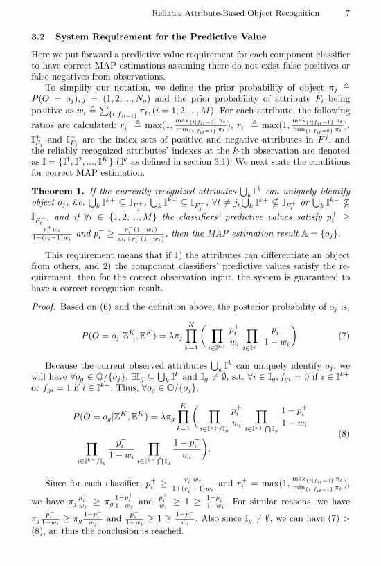
is assumed, then A = O′.Theorem 1 proves the system’s correctness under correct observations. Next,

for the general case section 3.3 proves that MAP estimation asymptotically con-verges to the actual result under certain assumptions.

3.3 Asymptotic Correctness of the MAP Estimation

Now we are going to prove that MAP estimation will converge to the correctresult when 1) the attribute classifiers’ PPV and NPV are high enough in theirreliable working region, where a lower bound of detection rate exists, and 2) theinputs are sampled randomly.

Denote di as the detection rate and qi as the false-positive rate of the i-thattribute classifier when applying the high PPV threshold in its reliable workingregion. Similarly, for the high NPV threshold, si denotes the true negative rateand vi denotes the false negative rate.

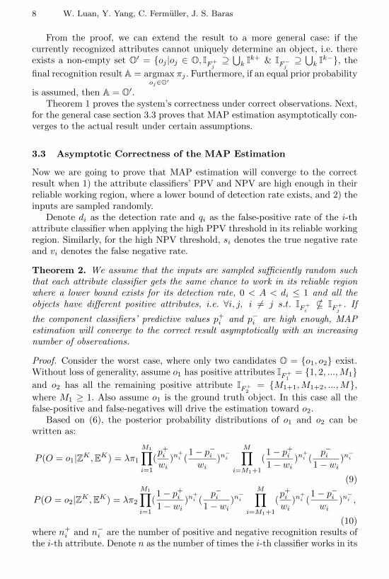
Theorem 2. We assume that the inputs are sampled sufficiently random suchthat each attribute classifier gets the same chance to work in its reliable regionwhere a lower bound exists for its detection rate, 0 < A < di ≤ 1 and all theobjects have different positive attributes, i.e. ∀i, j, i 6= j s.t. IF+

i* IF+

j. If

the component classifiers’ predictive values p+i and p−i are high enough, MAPestimation will converge to the correct result asymptotically with an increasingnumber of observations.

Proof. Consider the worst case, where only two candidates O = {o1, o2} exist.Without loss of generality, assume o1 has positive attributes IF+

1= {1, 2, ...,M1}

and o2 has all the remaining positive attribute IF+2

= {M1+1,M1+2, ...,M},where M1 ≥ 1. Also assume o1 is the ground truth object. In this case all thefalse-positive and false-negatives will drive the estimation toward o2.

Based on (6), the posterior probability distributions of o1 and o2 can bewritten as:

P (O = o1|ZK ,EK) = λπ1

M1∏i=1

(p+iwi

)n+i (

1− p−iwi

)n−i

M∏i=M1+1

(1− p+i1− wi

)n+i (

p−i1− wi

)n−i

(9)

P (O = o2|ZK ,EK) = λπ2

M1∏i=1

(1− p+i1− wi

)n+i (

p−i1− wi

)n−i

M∏i=M1+1

(p+iwi

)n+i (

1− p−iwi

)n−i ,

(10)where n+i and n−i are the number of positive and negative recognition results ofthe i-th attribute. Denote n as the number of times the i-th classifier works in its


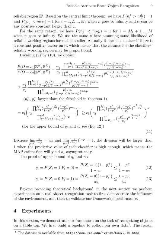
reliable region Ei. Based on the central limit theorem, we have P (n+i > ndiα ) = 1

and P (n−i < nαvi) = 1 for i = 1, 2, ...,M1 when n goes to infinity and α can beany positive constant larger than 1.

For the same reason, we have P (n+i < nαqi) = 1 for i = M1 + 1, ...,Mwhen n goes to infinity. We use the same n here assuming same likelihood ofreliable working regions for each classifier. Actually it does not matter if there isa constant positive factor on n, which means that the chances for the classifiers’reliably working region may be proportional.

Dividing (9) by (10), we obtain:

P (O = o1|ZK ,EK)

P (O = o2|ZK ,EK)=π1π2

∏M1

i=1(p+i /wi

(1−p+i )/(1−wi))n

+i (

(1−p−i )/(wi)

p−i /(1−wi))n−i∏M

i=M1+1(p+i /wi

(1−p+i)/(1−wi) )n+i (

(1−p−i )/wi

p−i /(1−wi))n−i

≥ π1π2

∏M1

i=1(p+i /wi

(1−p+i )/(1−wi))n

diα (

(1−p−i )/(wi)

p−i /(1−wi))nαvi∏M

i=M1+1(p+i /wi

(1−p+i)/(1−wi) )nαqi

(p+i , p−i larger than the threshold in theorem 1)

= c1

(c2

∏M1

i=1(p+i

1−p+i)d1α (

1−p−ip−i

)αvi∏Mi=M1+1(

p+i1−p+i

)αqi

)n≥ c1

(c2

∏M1

i=1(p+i

1−p+i)Aα (

1−p−ip−i

)α

1−p−i

wi

∏Mi=M1+1(

p+i1−p+i

)α

(1−p+i

)

1−wi

)n(for the upper bound of qi and vi see (Eq. 12))

(11)

Because limp→1

p1−p = ∞ and lim

p→1( p1−p )1−p = 1, the division will be larger than

1 when the predictive value of each classifier is high enough, which means theMAP estimation will yield o1 asymptotically.

The proof of upper bound of qi and vi:

qi = P (Zi = 1|Fi = 0) =P (Zi = 1)(1− p+i )

1− wi≤ 1− p+i

1− wi(12)

vi = P (Zi = 0|Fi = 1) =P (Zi = 0)(1− p−i )

wi≤ 1− p−i

wi(13)

Beyond providing theoretical background, in the next section we performexperiments on a real object recognition task to first demonstrate the influenceof the environment, and then to validate our framework’s performance.

4 Experiments

In this section, we demonstrate our framework on the task of recognizing objectson a table top. We first build a pipeline to collect our own data1. The reason

1 The dataset is available from http://ece.umd.edu/~wluan/ECCV2016.html

http://ece.umd.edu/~wluan/ECCV2016.html

http://ece.umd.edu/~wluan/ECCV2016.html


for collecting our own data is that other available RGBD datasets [14],[15] focuson different aspects, usually pose or multiview recognition, and do not containa sufficient amount of samples from varying observation distances.

Three experiments are conducted to show 1) the necessity of incorporatingenvironmental factors (the recognition distance in our case) for object recog-nition; 2) the performance of the high predictive value threshold classifier incomparison to the single threshold one; and 3) the benefits of incorporating lessdiscriminative attributes for extending the working range of classifiers.

4.1 Experimental Settings

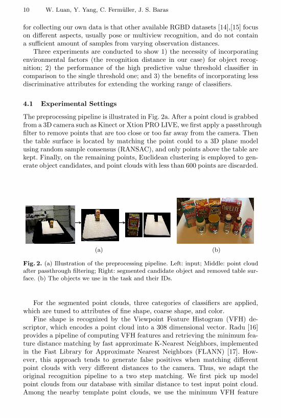
The preprocessing pipeline is illustrated in Fig. 2a. After a point cloud is grabbedfrom a 3D camera such as Kinect or Xtion PRO LIVE, we first apply a passthroughfilter to remove points that are too close or too far away from the camera. Thenthe table surface is located by matching the point could to a 3D plane modelusing random sample consensus (RANSAC), and only points above the table arekept. Finally, on the remaining points, Euclidean clustering is employed to gen-erate object candidates, and point clouds with less than 600 points are discarded.

(a) (b)

Fig. 2. (a) Illustration of the preprocessing pipeline. Left: input; Middle: point cloudafter passthrough filtering; Right: segmented candidate object and removed table sur-face. (b) The objects we use in the task and their IDs.

For the segmented point clouds, three categories of classifiers are applied,which are tuned to attributes of fine shape, coarse shape, and color.

Fine shape is recognized by the Viewpoint Feature Histogram (VFH) de-scriptor, which encodes a point cloud into a 308 dimensional vector. Radu [16]provides a pipeline of computing VFH features and retrieving the minimum fea-ture distance matching by fast approximate K-Nearest Neighbors, implementedin the Fast Library for Approximate Nearest Neighbors (FLANN) [17]. How-ever, this approach tends to generate false positives when matching differentpoint clouds with very different distances to the camera. Thus, we adapt theoriginal recognition pipeline to a two step matching. We first pick up modelpoint clouds from our database with similar distance to test input point cloud.Among the nearby template point clouds, we use the minimum VFH feature


matching distance as the classification score. Both steps use FLANN to accel-erate neighbor retrieval, where the former step uses the Euclidean distance andthe latter the Chi-Square distance.

As another type of attribute, we use coarse shape, which is less selective thanthe fine shape attribute. Our experiments later on demonstrate its advantage ofhaving a larger working region, thence it can help increase the system’s recog-nition accuracy over a broader range of distance. Two coarse shapes, cylindersand planar surfaces, are recognized by fitting a cylindrical and a plane model,whose coefficients are estimated by RANSAC. The percentage of outlying pointsis counted as the classification score for the shape. Thus, a lower score indicatesbetter coarse attribute fitting in our experiment.

The last type of attribute in our system is color, which is used to augmentthe system’s recognition capability. To control the influence of illumination, allsamples are collected under one stable lighting condition. The color histogramis calculated on point clouds after Euclidean clustering, where few backgroundor irrelevant pixels are involved. The Hue and Saturation channels of color arediscretized into 30 bins (5 × 6), which works well for differentiating the majorcolors.

As shown in Fig. 2b, there are 9 candidate objects in our dataset. To recognizethem, we use 5 fine shape attributes: shape of cup, bottle, gable top carton, widemouse bottle, and box; 2 coarse shape attributes: cylinder and plane surface; 3major colors: red, blue and yellow. The attributes for all objects are listed inTable 1. In the following experiments, we fix the pose of objects, and set therecognition distance as the only changing factor.

ObjectID

planesurface

cylinder

gabletop

cartonshape

boxshape

widemouthbottleshape

cupshape

bottleshape

redcolor

bluecolor

yellowcolor

1 X - X - - - - - X -2 X - X - - - - X - -3 X - X - - - - - - X4 X - - X - - - X - -5 - X - - X - - - - -6 - X - - - X - - X -7 - X - - - - X - - X8 - X - - - - X X - -9 - X - - - - X - X -

Table 1. Object IDs and their list of attributes

4.2 Experimental Results

EXPERIMENT ONE: The first experiment is designed to validate our claimthat the classifiers’ response score distributions are indeed distance variant.Therefore, it is necessary to integrate distance in a robust recognition system.


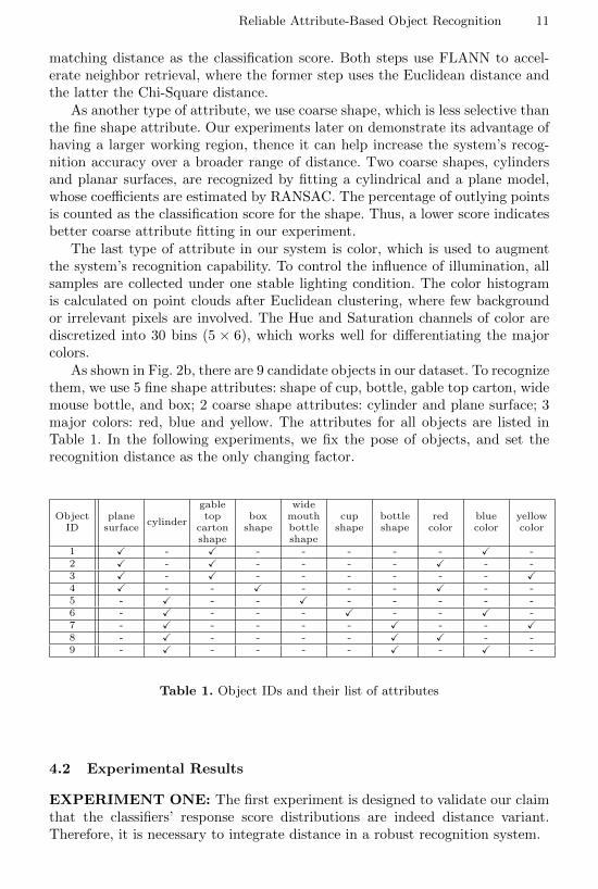
Taking the fine shape classifier of bottle shapes as example, we divide thedistance range between 60 cm and 140 cm into 4 equally separated intervalsand collect positive samples (object id 7, 8, 9) and negative samples from theremaining 9 objects in each distance interval. The number of positive samples ineach interval is 120 with 40 objects from each positive instance, while the numberof negative samples is 210 with 35 from each instance. The distribution of thebottle classifier’s response score is approximated by Gaussian kernel densityestimation with a standard deviation of 3, and plotted in Fig. 3.

Response score

0 50 100 150 200

Pro

babi

lity

dens

ity

0

0.01

0.02

0.03

0.04

0.05

0.06

0.07Recognition distance from 60 to 80cm

positive class

negative class

(a)

Response score

0 50 100 150 200

Pro

babi

lity

dens

ity

0

0.01

0.02

0.03

0.04

0.05

0.06


positive class

negative class

(b)

Response score

0 50 100 150 200

Pro

babi

lity

dens

ity

0

0.01

0.02

0.03

0.04

0.05

0.06


positive class

negative class

(c)

Response score

0 50 100 150 200

Pro

babi

lity

dens

ity

0

0.01

0.02

0.03

0.04

0.05

0.06


positive class

negative class

(d)

Fig. 3. Estimated distribution of bottle shape classifier’s response score under 4 recog-nition distance intervals.

We observe that the output score distribution depends on the recognitiondistance interval. Therefore, relying on one single classification threshold acrossall the distance intervals would introduce additional error. More importantly, weobserve that with a larger distance, the area of overlap between the positive andnegative distributions, becomes wider, which makes classification more difficult.

EXPERIMENT TWO: Experiment one demonstrated the difficulty oflearning a distance-variant ground truth distribution and corresponding classifi-cation thresholds. Therefore, we propose to use two high predicative value thresh-olds when multiple inputs are available. The second experiment is designed tovalidate this idea by comparing the classification accuracy of an estimator that1) uses two high predicative value thresholds, with an estimator that uses 2) oneoptimal Bayes threshold minimizing the error in the training data.


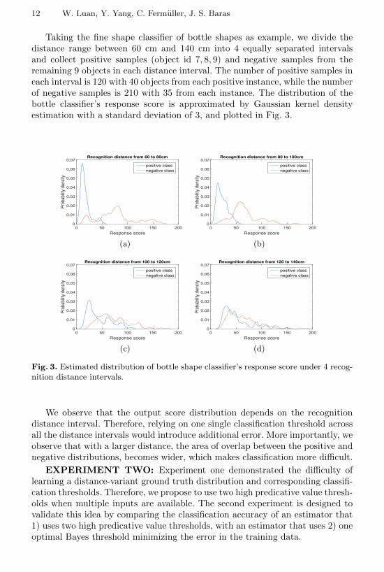
To have a fair comparison, we set our task as recognizing 5 objects (id1, 4, 5, 6, 9 ) with 5 fine shape attributes such that each object contains onepositive attribute that uniquely identifies it. Both training and testing pointclouds are collected at a distance of 100 cm to 120 cm . To learn the classifica-tion threshold, we sample 26 point clouds for each object and uniformly select20 for training. The testing data for each object consists of 22 point clouds thatwe can randomly choose from to simulate the scenario of an active moving ob-server gathering multiple inputs. Here we want to mention a special case. Whenour framework is uncertain based on the current input, it randomly select (withequal probability) one of the possible objects. The classification accuracy be-tween using a single threshold and using two high predicative value thresholdsare shown in Fig. 4a respectively.

We can see that both methods’ error rates decrease when the number of ob-servations increases. The approach using two thresholds (the red line) has lowererror rate than the one using a single threshold (the blue line). The green lineshows the error introduced by random selection, when our framework cannotmake a sole decision. The major part of the error in the two thresholds methodis due to this error. It is worth mentioning that under theoretical conditions, theclassical Bayes single threshold should still be the best in minimizing the clas-sification error. Our method provides an alternative for cases when the trainingdata in real world scenarios does not represent well the underlying distribution.

Number of observation

0 2 4 6 8 10 12 14 16

Err

or

rate

0

0.05

0.1

0.15

0.2

0.25

0.3

0.35

0.4

0.45

Single optimal threshold

Two high predictive value thresholds

Two thresholds w.o. certain decision

(a)

Distance interval (cm)

60-80 80-100 100-120 120-140 140-160

Acc

urac

y

0

0.2

0.4

0.6

0.8

1

Fine shape, color

Coarse shape, color

Fine, coarse shape, color

(b)

Fig. 4. (a): Error rate using classification with a single threshold (blue) and two highpredictive value thresholds (red). The green line depicts the error component due tothe cases where the two thresholds method has to randomly select. (b) Three systems’recognition accuracy for different working distance intervals.

EXPERIMENT THREE: The third experiment demonstrates the ben-efits of using less discriminative attributes for extending the system’s workingrange. To recognize the 9 objects in Fig. 2b, we build three recognition systemsutilizing attributes of fine shape and color, coarse shape and color, and all of thethree attributes, respectively. Considering the influence of the recognition dis-tance on the response score distribution, the complete range of distances from60 cm to 160 cm is split into 5 equal intervals. We then learn the classifica-


tion thresholds and predictive values accordingly. Both, the training and thetesting data, consist of around 100 samples from each object across recognitiondistances from 60 cm to 160 cm. We learn the PPV and NPV by counting thetraining data w.r.t. the thresholds and select thresholds satisfying a predictivevalue larger than 0.96. The minimum detection rate for the reliable workingdistance interval is 0.09. This means if 1) an attribute classifier cannot find athreshold with PPV larger than 0.96, and 2) detection rate larger than 0.09 ina certain distance interval, the output of this attribute classier in this intervalwill not be adopted for decision making. During the testing phase, for fair com-parison, we constrain the number of input point clouds collected from the samedistance interval in each working region. Around 120 point clouds are collectedfor each object. Once more, random selection is applied when multiple objectsare found as possible candidates.

Fig. 4b displays the systems’ recognition accuracy after observing three timesin each distance interval. As expected, the classification performance starts todecrease for larger distances. At 120 cm to 160 cm, the system using fine shapeattributes (blue) performs even worse than the system using less selective coarseattributes (green). This validates that the coarse shape based classifier has alarger working region, though its simple mechanisms allows for less discrimina-tion than the fine grain attribute based classifier. Finally, due to the comple-mentary properties, the system using all attributes (yellow) achieves the bestperformance at each working region.

5 Conclusions

In this work we put forward a practical framework for using multiple attributesfor object recognition, which incorporates recognition distance into the deci-sion making. Considering the difficulties of finding a single best classificationthreshold and the availability of multiple inputs at testing time, we propose tolearn a high PPV and a high NPV threshold and discard uncertain values duringdecision making. The framework’s correctness was proven and a fundamental ex-periment was conducted to demonstrate our approach’s feasibility and benefits.Additionally, we showed that less selective shape attributes (compared to thesophisticated ones) can have advantages, because their simple mechanism canlead to high reliability when the system is working at a large range of distances.

In future work, we plan to extend the approach to a variety of environmentalfactors such as lighting conditions, blur, and occlusions. Furthemore, additionalattribute classifiers will be incorporated to improve the system’s recognitionperformance.

Acknowledgment: This work was funded by the support of DARPA(through ARO) grant W911NF1410384, by NSF through grants CNS-1544787and SMA-1540917 and Samsung under the GRO program (N020477, 355022).


References

1. Kanezaki, A., Marton, Z.C., Pangercic, D., Harada, T., Kuniyoshi, Y., Beetz, M.:Voxelized Shape and Color Histograms for RGB-D. In: IEEE/RSJ InternationalConference on Intelligent Robots and Systems (IROS), Workshop on Active Se-mantic Perception and Object Search in the Real World, San Francisco, CA, USA(September, 25–30 2011)

2. Xie, Z., Singh, A., Uang, J., Narayan, K.S., Abbeel, P.: Multimodal blendingfor high-accuracy instance recognition. In: Proceedings of the 26th IEEE/RSJInternational Conference on Intelligent Robots and Systems (IROS). (2013)

3. Lutz, M., Stampfer, D., Schlegel, C.: Probabilistic object recognition and poseestimation by fusing multiple algorithms. In: Robotics and Automation (ICRA),2013 IEEE International Conference on. (May 2013) 4244–4249

4. Salih, Y., Malik, A.S., Walter, N., Sidibe, D., Saad, N., Meriaudeau, F.: Noiserobustness analysis of point cloud descriptors. In: 15th International Conferenceon Advanced Concepts for Intelligent Vision Systems - Volume 8192. ACIVS 2013,New York, NY, USA, Springer-Verlag New York, Inc. (2013) 68–79

5. Wu, T., Zhu, S.C.: Learning near-optimal cost-sensitive decision policy for objectdetection. In: IEEE International Conference of Computer Vision. (2013)

6. Lowe, D.G.: Distinctive image features from scale-invariant keypoints. Interna-tional Journal of Computer Vision 60 (2004) 91–110

7. Xu, Y., Ji, H., Fermuller, C.: A projective invariant for textures. In: ComputerVision and Pattern Recognition, 2006 IEEE Computer Society Conference on.Volume 2. (2006) 1932–1939

8. Bertsche, M., Fromm, T., Ertel, W.: Bor3d: A use-case-oriented software frame-work for 3-d object recognition. In: Technologies for Practical Robot Applications(TePRA), 2012 IEEE International Conference on. (April 2012) 67–72

9. Hinterstoisser, S., Lepetit, V., Ilic, S., Holzer, S., Bradski, G.R., Konolige, K.,Navab, N.: Model based training, detection and pose estimation of texture-less 3dobjects in heavily cluttered scenes. In: Computer Vision - ACCV 2012 - 11th AsianConference on Computer Vision, Daejeon, Korea, November 5-9, 2012, RevisedSelected Papers, Part I. (2012) 548–562

10. Attamimi, M., Mizutani, A., Nakamura, T., Nagai, T., Funakoshi, K., Nakano, M.:Real-time 3d visual sensor for robust object recognition. In: Intelligent Robotsand Systems (IROS), 2010 IEEE/RSJ International Conference on. (Oct 2010)4560–4565

11. Collet Romea, A., Martinez Torres, M., Srinivasa, S.: The MOPED framework:Object recognition and pose estimation for manipulation. International Journal ofRobotics Research 30(10) (September 2011) 1284 – 1306

12. Fromm, T., Staehle, B., Ertel, W.: Robust multi-algorithm object recognition usingmachine learning methods. In: Multisensor Fusion and Integration for IntelligentSystems (MFI), 2012 IEEE Conference on. (Sept 2012) 490–497

13. Naguib, A., Lee, S.: Adaptive bayesian recognition with multiple evidences. In:Multimedia Computing and Systems (ICMCS), 2014 International Conference on.(April 2014) 337–344

14. Lai, K., Bo, L., Ren, X., Fox, D.: A large-scale hierarchical multi-view rgb-dobject dataset. In: Robotics and Automation (ICRA), 2011 IEEE InternationalConference on. (May 2011) 1817–1824

15. Singh, A., Sha, J., Narayan, K.S., Achim, T., Abbeel, P.: Bigbird: A large-scale 3ddatabase of object instances. In: Robotics and Automation (ICRA), 2014 IEEEInternational Conference on. (May 2014) 509–516


16. Rusu, R.B., Bradski, G., Thibaux, R., Hsu, J.: Fast 3d recognition and pose usingthe viewpoint feature histogram. In: Proceedings of the 23rd IEEE/RSJ Inter-national Conference on Intelligent Robots and Systems (IROS), Taipei, Taiwan(10/2010 2010)

17. Muja, M., Lowe, D.G.: Scalable nearest neighbor algorithms for high dimensionaldata. Pattern Analysis and Machine Intelligence, IEEE Transactions on 36 (2014)

Documents

Reliable Attribute-Based Object Recognition Using High …yezhouyang.engineering.asu.edu/wp-content/uploads/2016/08/ECCV20… · Reliable Attribute-Based Object Recognition 3 (a)