Reliability Models to Predict Engineering Systems ... · Reliability Models to Predict Engineering Systems 'Failures and Improve their Performance Amal El-Berry 1, and Afrah Al-Bossly2

Reliability Models to Predict Engineering Systems 'Failures and Improve their

Performance Amal El-Berry 1, and Afrah Al-Bossly2

1 Mechanical Engineering Department, National Research Center, Cairo, Egypt Faculty of Engineering &Computer Science, Prince Sattam Bin Abdulaziz University, KSA.

2Mathmatics Department, Faculty of Science and Humanities Studies, Prince Sattam Bin Abdulaziz University, KSA.

Abstract- In electronic devices systems, the average lifetime could be expected based on handling enormous populations of components probabilistically. Time dependency of reliability was understood by the description, and therefore the time variables appeared in all of the failure distribution purposes that would be consequently. The research will be a specified test system or operating conditions that are necessary to predict reliability. At start of study COMSOL Multiphysics Modeling Software to solve model which indicated the effect of higher temperature by climate or run on the electronic chip. To demonstrate the reason, which may cause the collapse of the device, especially in the country where the climate was hot at certain times of the year such as one of the reasons public and which accelerate the collapse of the systems. Electronic devices had a big difference when tested under the influence of temperature. Significant technical terms related to engineering reliability and having different significances were taking into consideration such as availability, maintainability, and survivability. Probability of collapse was a measured of the reform components will work for a while. Collapse consists of transition from reliability to the case of failure. Regardless of specific mechanism, failure almost always starts off by the movement of time independent of ions and atoms or electronic charge from the benign side to the harmful side. The main problem of the research was how to evaluate a good case for electronic devices operating system by estimating reliability. Data analyzed with support Weibull++/ALTA 9 and BlockSim 9 software and algorithms reliability. Sample reliability with the appropriate had been estimated input parameters for this models (such as failure rates for non-specific situation or event and at the same time to reform the system for the failure of a particular). To provide a system (or part) to estimate the level of reliability of the output parameters (Availability of the system or frequency specific functional failure). Some probability distributions had been presenting such as Weibull, Gumbel and gamma .A comparison between the different distributions to ensure the effectiveness of one of them to determine the reliability of engineering and electronics systems would be derived authority functions and features of the distribution of thermal stress also. Finally cost factors was used to estimate the target reliability for a product and calculate the return on an investment intended to influence that reliability.

Keywords: Cost ;Finite element; Gamma; Gumbel; Modeling; Overheating; Reliability; Weibull. 1. INTRODUCTION

Imbalance of phase current caused neutral current in three phase power systems. The neutral currents were very high. The neutral current problem was discussed with the help of sample computer power systems. The remedies due to this problem was also discussed by Thomas M.Gruzs[1]. In V. M. Dwyer et al.[ 2 ]’ work an defect of random geometry was examined and subjected to arbitrary profile , the problem of thermal runaway was observed. The rectangular parallel piped geometry was identified as having the ability to model the defects arising in semiconductor device. Apart from the previous work, full range of values was used by all three dimensions. In contradiction to the earlier theories this theory proved that there four time domains and it existed for all shapes. Hong Xie et al. [3] reviewed the design of 6.5 W of CPU power to solve thermal fatigue. They applied four solutions to this reference notebook. They were heat pipe connected to keyboard, heat sink and the aluminum plate solution, Heat pipe to connected outside, and fan heat sink solution. Though the research was carried out only for reference notebook but it can be extended to general notebook. Vladimir Szekely et al. [4] proposed the thermal stimulators finite element model. They made a study on the effect of heat on working of integrated circuits. They initiated a simulation of the electrical network scheme. The simulation derived the thermal parameters. In turn these parameters were useful in building up model network for the thermal part. They stimulated the coupled system. A study of the surface thermal fatigue of electrical components was conducted by S.Dilhaire et al. [5].The study was conducted at 4, 43, and 70 and 130 minutes respectively once the die was cooled to room temperature. From the results the initial bending amplitude was identified as 0.5~tm [5]. M. Gall et al. [6] detected failures in electro migration with experimental and theoretical methods and

Amal El-Berry et al. / International Journal of Engineering and Technology (IJET)

ISSN : 0975-4024 Vol 7 No 3 Jun-Jul 2015 894

results proved the fact, that electro migration failure followed perfect long normal behavior down to four sigma level. John H. Pang et al.[7] have been correlated life flip chip solder to predict thermal parameters which affect joint' fatigue. Data center consists of many racks with multiple microprocessors. Large amount of heat is dissipated from such racks. Cooling design infrastructure depending on the layout of racks can save energy. Chandrakant D et al. [8]’ paper illustrates a data center cooling design and seduces a numerical model for changing the layout to make air-conditioning resources usage efficient. Ching-Kong Chao et al. [9] measured the temperature during the cooling process with finite difference method. Induced thermal stresses during cooling process were calculated using trapezoidal integration technique. Convective cooling in the initial stage is not advisable. Regarding radiative cooling the temperature non uniformity was caused by edge effect and geometric relation between chamber and wafer. The temperature non uniformity in the wafer caused by edge effect is discussed in this paper. The work aims at determining a mathematical model under rapid thermal processing to obtain the temperature distribution and thermal stress throughout the wafer. Ryan J et al. [10] have engineered the design of initial heat exchangers for electronic component cooling. Computational fluid dynamics (CFD) analysis was performed and simple comparisons of thermal performance were made and thus the channel was designed. The mathematical models were proposed for the heat exchanger designs under the condition of different flow rates. Comparisons were made with test results under various conditional factors such as changed fluid flow rate, varied heat source power level, environmental temperature and inlet fluid temperature. The electronic devices are usually designed using commercial-off-the-shelf components with known cost and reliability. However, some component characteristics, such as the failure rate, exhibit significant, unit-to-unit variability, The LHS method was used by E.P. Zafiropoulos, E.N [11]. A. Sittithumwat et al [12] established assuming constant failure rates for the components and was extended to optimization given limited information about equipment condition reasoning using fuzzy. Advances in CMOS technology has enhanced processor performance. Improvement in CMOS was increasing power density and also processor temperature. In the deep sub-micron area the reliability effect of scaling was studied Jayanth Srinivasan et al [13]’ results. The strong challenges are due to TDDB (Time dependent dielectric breakdown) and electro migration. Results show how the scaling affects the failure rates. In a notebook computer the thermal loads were monitored by Nikhil Vichare et al. [14] for different environments. The effects of various factors like power cycles, usage history, CPU computing resource usage and external environment on internal peak transient thermal loads was characterized. The maximum temperature amplitude estimated surpassed environmental standards. Tests were performed according Weilin Qu and Issam Mudawar [15] for CHF for single mini-channels which unsteady flow instabilities induced vapor back flow into the heat sinks upstream plenum, which significantly altered the coolant temperature at the channel inlets. Yan Qi et al. [16] conducted experiments related to resistor solder joints. The stress and strain on solder joints caused by the influence of transient temperature gradients were simulated by finite element models. High ramp rate of 95 C min was set and temperature gradient was measured to be 7 C -11C all through the resistor thickness during ramp up and ramp down of temperature. The total von Mises strains and stresses in SnPb and SAC solder joint is found to be 1% less compared to a condition where in there is a uniform time varying temperature. In a high power microelectronic circuits which was connected to a heat sink, the radiation emitted was observed and finite-element frequency domain was presented by Junwei Lu and Francis Dawson[17] .A simulation model for Intel P4 CPU heat sink was developed and analyzed. Joseph B. Bernstein et al. [18] reviewed and a new failure rate-based SPICE reliability simulation methodology is proposed to address some limitations inherent in the former methods. Both types of simulation are based on the same wear out failure physics but addressing reliability from different perspectives. Bianca Schroeder and Garth A. Gibson [19] surveyed the failure information for compute clusters and storage systems. The research projects failure rates of elements and resulting decrease in effectiveness of application. The paper also discusses strategies to handle failure for supercomputers. There is a risk of excessive resource utilization on fault recovery methods due to the lagging of per chip computing power. There was an utmost need for repository of failure records to be publicized. Srinivasan Murali et al. [20] presented a novel convex optimization methods. It provided a solution to the problem of processor frequency assignment. The optimal frequency for processor could been fixed by this approach. Soon-Bok Lee and Ilho Kim[21] investigation about the fatigue life of cyclic bending test which showed linear relationship with damage parameters such as inelastic strain and dissipation energy, but the fatigue life acquired from thermal cycling test has non-linear relationship due to the thermal degradation. Electrical devices principal parameters can be used by M.A. Belaı¨d [22] to evaluate its reliability and lifetime, allowing correlation to be established between the electric parameter drift and the applied stress. Electronic power devices fail due to temperature variations. The chips in these devices were isolated from their base plates by DBC (Direct bonded copper) which fail due to large thermal amplitude. Geometric singularities are at the origin of cracks which grow in proportion to the fatigue and finally break. S. Pietranico et al. [23] showed that how framework of linear elastic fracture mechanism (LEFM) could predict the stress field circling the singularities and failure risk. The experiments proved that inducing three overload cycles (70 degree celcius+ 180degree celcius) prior to thermal fatigue cycles enhances the fatigue life of substrates. Hyung Beom Jang et al. [24] checked the architectural



effects such as temperature leakage and reliability of direct interlayer cooling method. The results proved that this scheme remarkably reduces on chip temperature. This in turn reduces leakage reduction which in turn enhanced the lifetime reliability. The efficiency of the liquid cooling scheme is evaluated. M. Diatta et al.[25] proven that repetitive ESD stresses on a safety device such as a bidirectional diode convince advanced failings into the silicon bulk. With ‘‘Sirtl etch” failure study technique, the weak spot could be localized quite accurately at the peripheral in/out joints. The degradation machines during repetitive IEC 61000-4-2 pulses had been considered on a safe-guard diode with the objective of refining the design for sustaining 1000 pulses at 10 kV level. The paper which proposed by Y. Q. Ni et al. [26] a fatigue reliability model was proposed by unifying continuous probabilistic formulation with hot spot stress range probability distribution. The PDF for stress range was generated and utilizing the finite element analysis method SCFs at fatigue prone points were estimated. With the help of the structural reliability theory a PDF of parameters such as failure probability and reliability index versus fatigue life was deduced. J. Virkki et al. [27] have been used method suits various reliability tests and facilitates effective comparison of components from different vendors. F. Hedrick et al.[28]. took up sleep respiration disturbances and their relation with cardiovascular diseases. A thermal flow sensor is used. The sensor exhibits high accuracy and short response time. On account of large amount of heat produced in the computer components there is an inevitable need to dissipate the heat in order to prevent failure due to shortage of lifetime as well as to avoid creating erratic problems causing system crashes and freezes. Cooling of the components by peripheral methods is carried out by heat sinks and air cooling fans. Here there is study made on comparison of traditional methods versus latest technology of cooling such as thermoelectric cooling. The effect of the time span on heat transfer between the components and processor temperature improvement were studied in detail. T. Abbas et al.[ 29 ]. Tsukasa Takahashi et al. [30] systematically investigated and compared the self-heating effects in Bulk/SOI FinFETs. Tsukasa studied the heat dissipation pathways in BULk/SOI FinFETS. Analysis was made on thermal characteristics device parameter dependence. Results prove that the effect of thermal resistance at the interface of MOS was more considerable in SOI FinFETs than in Bulk FinFETs. The two main reasons for cracks in materials is due to alternative caused due to temperature gradient and a process of cycling thermal load. The structure within the substrate is affected by the temperature gradient up to 600 ºC/cm. This causes the varying stress distribution. This high temperature gradient causes metal migration which in turn causes defects inside the solder ball and the cycling thermal loads convert defects to cracks and crack propagates through plastic deformation accumulation. The simulation results of Zheming Zhang and Jingshen [31] showed that the maximum stress was at the solder bump. Larisa Mariut [32]’s paper deals with effect of different voltage waveforms/frequencies and temperature gradient on partial discharge within cavities of power cable insulation. Under different testing conditions the behavior of partial discharge is studied. PD checked were conducted with AC, DC step and oscillating voltage waveforms at 50 Hz, Very Low Frequency (0.1 Hz/ VLF) .For insulation systems with embedded cavities the complete PD analysis was done. Studies showed that the temperature gradient within the cavities is dependent on frequency. The PD activity is affected by the presence of heat flux inside the cavity. M.-N. Sabry and M. Dessouky [33] presented a model to predict effect of heat and reliability of the downscaling semiconductor chips. Chuan Xu et al. [34] formulated the rigorous analytical thermal model and this model was helpful in estimating the thermal time constants of devices. The thermal time constants of devices are estimated with transient thermal model. The junction temperature of LEDs are monitored by diode forward voltage method. Pulsed current observed the thermal transient effect and errors were introduced. A direct junction temperature measurement method was carried out for HV LEDs to reduce errors. It was also useful in getting in situ junction temperature with dc currents, simple steps and a less step sequence followed Huaiyu Ye et al.[ 35]' study. Dragica Vasileska [36] discussed the self-heating effects and their implications on the operation of different generations of silicon on insulator devices. Wangcun Jia et al. [37] proposed an approach to show the thermal behavior in the structure of semiconductor integrated-circuit onto a functional space depending on proper orthogonal decomposition. Analysis of a cooling Power PC620 processor in an environment of multiprocessor computing system using passive heat sinks was done by Henry Wong et al.[38].In order to monitor and record the airflow and air temperatures at the system and board levels computational fluid dynamics software was utilized. Results from experiment calculated the junction temperature. According to the experimental results junction temperature can be maintained below 85“C for a 25 Watt processor and 100 “C for a 30 Watt processor with the support of compact heat exchanger. The problem of thermal runaway was observed by V. M. Dwyer et al. [39] the rectangular parallel piped geometry was identified as having the ability to model the defects arising in semiconductor device. Apart from the previous work, full range of values is used by all three dimensions. In contradiction to the earlier theories this theory proved that there four time domains and it exists for all shapes. Mitchell 0. Locks [40] proposed the application of Mann-MFS methodology for extreme value estimation and reliability confidence assessment, it found that difference in the interpretation of the term “confidence" between the Mann-MFS methodology and regression based or maximum likelihood techniques. Necip Doganaksoy et al. [41] proposed that there is no dependency between failure modes. Jayanth Srinivasan et al. [42]’experimental results clearly showed that effect of temperature on wear out driven (un)reliability and effect of degradation un reliability caused by technology



scaling alone, such as dielectric breakdown. G. Cassanelli et al. [43] determined methodology to minimize the deficiencies of the traditional reliability prediction methods calculating a corrective factor using the available field return data sets. Y.A. Chau and K.Y.-T. Huang [44] proposed a model for multivariate Weibull distribution. The probability density function of Weibull distribution was extracted and evaluation was made on the outage probability of selection diversity. The results were recorded and it showed that the failure rate of the system increased proportional to the processor chip quantity. The study also showed that there was not much chances of the hardware getting reliable over time. Srinivasan Murali et al. [45] presented a novel convex optimization methods. It provides a solution to the problem of processor frequency assignment. The optimal frequency for processor can be fixed by this approach. In order to detect multiple outliers in both large and moderate quantity data sets Sharmila Banerjee presented a univariate outlier identification method. This was based on the box-plot outlier labeling rule. Probability properties were derived mathematically Sharmila Banerjee and Boris Iglewicz [46]. D.W. Matolak et al. [47] examined the relationship between correlated Weibull RVs and coefficients of Rayleigh RVs. An algorithm was developed to generate the multivariate weibull RVs with random fading parameters based on the relationship. Tongdan jin and Lakshmana Gonigunta [48] produced a new method to calculate the Weibull or Gamma by using exponential function. K.S. Sultan et al. [49] had been test number of component by using mixture of two inverse Weibull distributions, likelihood ratio is computed in two criteria. It had been noted that to optimize the likelihood was not necessary to obtain a good results. Anduin E. Row [6] used a method to decrease the required number of numerical integrations and estimated from 5 to 2 Bayesian estimation on mixed Weibull situations. Govind S. Mudholkar [51] provided a new method to transform data, his approaches depend on using different distributions to calculate time to failure to analyze reliability of mechatronic systems. Software reliability Growth Models were developed by Quadri and N. Ahmad [52].Least square estimation technique was estimated to model parameters. The results were also compared with other models. This shows that proposed SRGM has better fault prediction capability.This model can be used for variety of software systems. Kahadawala Cooray et al. [53] presented a two parameter family of distribution. There were many common distributions such a lognormal, log logistic, inverse Gaussian, inverse Weibull, Weibull and etc.to model reliability data. Inverse Weibull-Weibull composite family is one of the best for reliability analyst .The reason for this is its flexibility of estimating parameters and convenience of testing. To compare and forecast the applicability of proposed distribution a real data illustration related to repair times is given. To improve product quantity and reliability the new approach was designed by Laura J. Freeman and Geoffrey [54].The analysis proposed can be conducted on Minitab and similar statistical packages. The field failure data was analyzed by B. Hari prasad et al. [55] and the reliability predictions of vehicles was explained. Single layer perceptron model demonstrated for enhancing the accuracy of the reliability values. Computational effort increases with addition of hidden layers ANN layers. Implementation is done by RDBMS.

2. MODELS AND METHODS

2.1 Heat Effect on Electronic Component The model layout as in Fig. 1 consisted of silicon chip, aluminum pins, FR4 board, copper ground plane and

interconnection taken as component in system may be failure because it subjected to hot spots temperature increase. Study considered the effect of heat transfer in silicon chip by conduction by the conducted heat and this may lead to overheating of the chip according to heat transfer in solids Eq. (1).

Fig. 1 Silicon chip mounted on FR4 board

+ . + . (− ) = (1)

Where: ρ = Density (kg/m3) Cp = Heat capacity (J/ (kg·K)) k = Thermal conductivity u = Velocity field



Q = Heat source The thermal conductivity defined the correlation concerning the heat flux vector field q where temperature = gradient ∇T q = −k∇T "Fourier’s law of heat conduction". The heat capacity at constant pressure defined the quantity of heat energy requisite to products a unit temperature variation in a unit mass. In adding, the thermal diffusivity α, defined as k ⁄ (ρ Cp) (m2/s), was also a predefined quantity. The thermal diffusivity could be interpreted as a measure of thermal inertia. The components of the thermal diffusivity α. The initial Values node adds an initial value for the temperature that could aid as an initial condition for a transient simulation. A value or expression for the initial value of the temperature T (K). The default value was nearly room temperature, 293.15 K (20 ºC).The thermal insulation node was the default boundary condition for all heat transfer edges. This boundary condition means that there was no heat flux across the boundary: . ( ) = (2) and hence requires where the area would isolated. Naturally, Eq. (2) detailed the temperature incline crossways the boundary was (0). For this to be accurate, the temperature on one side of the boundary requirement equal the temperature on the other side. Because there was no temperature difference crossways the boundary, heat cannot transfer crossways it. If thermal insulation was selected, no heat exchange occurs between the two adjacent domains at both sides of the boundary. The impervious surface node definite a boundary impervious to radiation. The impervious surface node described event intensities on a boundary and accounts for the net radiative heat flux, qw that was absorbed by the surface. The impervious surface node was available for the heat transfer with radiation in contributing media interface version of the heat transfer interface. It was also available for the radiation in contributing media interface. There was one standard model input—the temperature T the default was 293.15 K and was used in the blackbody radiative intensity expression. If gray wall was selected the default surface emissivity ε value was taken from material (a material defined on the boundaries). An emissivity of 0 means that the surface emits no radiation at all and that all outgoing radiation was diffusely reflected by this boundary. An emissivity of 1 means that the surface was a perfect blackbody, outgoing radiation was fully absorbed on this boundary. Radiative intensity (W/m2) along incoming discrete directions on this boundary was defined by: , = ( ) + (3)

If dark wall was selected, the radiative intensity along the received discrete instructions on this boundary was definite by: , = ( ) (4) Values of radiative intensity along departing disconnected directions are not approved. ε = Radiative heat flux at the boundary depends on the surface emissivity I (T) = "Blackbody radiation intensity" When isolated ordinates technique selected, the continuity on interior boundary node enables intensity conservation across internal boundaries. It was the default boundary condition for all internal boundaries. The Heat Source defined heat generation within the domain. Add one or more nodes as required—all heat sources within a domain contribute to the total heat source. Specify the heat source as the heat per unit volume, as a linear heat source, or as a heat rate. Linear source in Eq. (5) was selected, production/absorption coefficient qs (W/(m3·K)). The default was 0 W/ (m3·K). (Q=qs·T) (5)

If General inward heat flux q0 (W/m2) was selected, it adds to the total flux crossways boundaries. q0 characterized a heat flux that enters the domain. The default was 0 W/m2.External temperature, Text (K). The default was 293.15 K. The value depended on the geometry and the ambient flow conditions. Convective heat flux was definite by: q0 = h (Text − T) (6)

Use the Thin Layer feature to define thermal and thickness properties of a thermally resistive material layer located on boundaries. With the addition of the Heat Transfer Module, also model heat transfer in thin greatly conductive layers.The thin conducting layers of the ground plane and interconnect within the package is modeled using a 2D shell approximation, according to: . (− ) = (7) where ds was the layer’s thickness, and ∇t represents the nabla operator expected onto the direction of the plane. The model used a Heat Transfer interface to describe the 3D heat transfer as well as the 2D shell heat transfer.A model was solved by computing a solver configuration—a scheme for computing a solution loosely speaking a



solver configuration consists of one or more solution nodes, and each Solution node consists of a sequence of sub nodes specifying how to compute the solution. Typically, such a solver configuration contains information about which physics interface and geometry to use, which variables to solve for, and which solvers to use for the type of study to perform. Meshing sequences to the Component. When a Component has more than one meshing sequence, they are collected under a meshes node. It was used to compute static electric or magnetic fields, as well as direct currents. In heat transfer, it was used to compute the temperature field at thermal equilibrium. In solid mechanics, it was used to compute deformations, stresses, and strains at static equilibrium. In fluid flow it was used to compute the steady flow and pressure fields. 2.2 ELECTRONIC DEVICES’ RELIABILITY, RISK RATE AND MTTF

Functions Numerous universal functions used in performance reliability analysis. 3 of these functions were obtainable

below: 2.2.1 Universal Reliability Function: This was determined by: ( ) = ( ) (8) Eq. (8) expressed for the universal reliability function. It used to achieve the reliability of an element whose times to failure defined by statistical distributions such as Weibull, exponential, normal and Rayleigh. Where: R (t) = Reliability "at time t" λ (t) = "Risk rate or time-dependent failure rate" 2.2.2 Risk Rate Function

Risk rate function expressed as: ( ) = ( )( ) (9)

Or ( ) = ( ) . ( ) (10)

f (t) was the failure (or probability) density function 2.2.3 Mean Time to Failure

Mean time to failure could be achieve using any of the following formulas: = ( ) (11)

Or = → ( ) (12) Or = ( ) (13) MTTF = "mean time to failure" s = "Laplace transform variable" R(s) = "Laplace transform of the reliability function, R (t)" 2.3 Reliability for Electronic Devices Networks

An electronic devices system could formula several styles of systems or structures in performance reliability investigation. Some generally occurring conformations were obtainable as follow: 2.3.1 SERIES CONNECTION

This was possibly the greatest usually happening configuration in engineering systems. Each block in the diagram denoted a element or component. In this preparation or construction, all the units must activate usually for the active operation of the system (i.e., the series system).Let Xj denoted the event that the jth unit was successful, then the reliability of the series conformation/system given by: = ( …… . ) (14) Where Rs was the series system or configuration reliability ( …… . ) Was the existence probability of success events …… . For independent units, Eq. (14) becomes: = ( ) ( ) ( )…… . ( ) (15) Where: P(Xj) was the probability of manifestation of success event Xj, for j = "1,2,3,…….,n"



If let Rj = "P(Xj) ; for j=1,2,3,……….,n." = ∏ (16) = "unit j reliability; for j=1,2,3,……….,n" For constant failure rate, of unit j, using Eq. (8) the reliability of unit j given by: ( ) = = (17) Where: ( ) = Reliability of unit j at time t Substituting Eq. (16) into Eq. (17) ( ) = ∑ (18) ( ) = Reliability of the series system at time t. Inserting Eq. (13) into Eq. (17) we get = ∑ = ∑ (19)

Where MTTFs was the series system mean time to failure. 2.3. 2 Parallel Connection

Total n elements were active and at least one of these elements must function normally for the effective task of the system. The block diagram of an “n” unit parallel formation/system was shown in each block in the diagram characterized a unit.

Signify the event that the jth unit was failed, then the failure probability of the parallel system/conformation was given by: = ( …… . . ) (20) Where Fp was the parallel system/conformation reliability, ( …… . . ) Was the occurrence probability of failure events …… . . . For independent units, Eq. (20) becomes: = ( ) ( )…… . . ( ) (21) Where

= "manifestation probability of failure event ; for j = 1, 2, 3,………..n"

If we let = 1,2, ………… . . , = ∏ (22) Where Fj = "failure probability of unit j; for j = 1, 2,… ……..n"

Subtracting Eq. (3-9) from unity achieved: = −∏ (23) Where Rp = "parallel system/conformation reliability" For the constant failure rate, of unit j, subtracting Eq. (17) from unity; then, Substituting it into Eq. (22) yields: ( ) = −∏ ( − ) (24) Where Rp(t) = parallel system/conformation reliability at time t. For identical units, using Eq. (11) and (24) we get = − ( − ) = ∑ (25)

Where = unit constant failure rate,

MTTFp = parallel system/conformation mean time to failure.



2.3.3k-out-of-n Connection

N number of elements were active and at least k units essential activate generally for the system success. The parallel and series connections were special cases of this configuration for k = 1 and k = n, respectively. Using the binomial distribution, for independent and same units, expressed as next for the k-out-of-n conformation reliability:

/ = ∑ ( − ) (26)

Where: = !( )! ! , R / = the k-out-of-n configuration/system reliability, R = the unit reliability. For constant failure rates of units, using Eqs. (8) and (27) we get

/ ( ) = ∑ ( − ) (27)

Where / ( ) ="k-out-of-n configuration/system reliability at time t" = "unit constant failure rate"

Substituting Eq. (27) into Eq. (1) we get:

/ = ∑ ( − ) = ∑ (28)

Where MTTF / = "mean time to failure of the k-out-of-n configuration/system" The study indications parameter that estimations for three universally consistent methods: the standard

Gamma, Gumbel and 2p-Weibull distributions. Viewing fitting of the previous models, as listed for a time–to–failure. The frequently used method in reliability modelling was to model the time between failures as a random variable. The estimation of future performance of the observed system, it expected that the time between failures could demonstrated as a 2p- Weibull distributed random variable, with and reliability Rt and probability density function f(t), also cumulative density function. Availability A(t) and maintainability were determined to optimize the true maintenance time for the system. The usage of the Gamma and Gumbel distributions still had approximately value to reliability investigation. As more of a concession than the standard, the distributions could be efficiently merge into reliability investigation if the constant failure rate supposition could be justified. In addition, earlier efforts and standards that expansively developed the exponential distribution should be commend for presenting and formalizing the reliability methods that formed the basis of more advanced investigation methods and for applying more severe scientific approaches within the field. Comparison between two distributions was perform to optimize proposed method.

3. RESULTS AND DISCUSSION

Overheating chip FEM simulation leading to the rapid collapse of the electronic device. Maximum, Average, or minimum were compute of any amount to calculate resulting amounts. To describe estimations of arithmetical results—generally, in a fact, or integrated amounts. For 2D and 3D schemes, also got arithmetic results. For all derivative principles had been also apply an operator on a data sequence to calculate, the temporal average of an amount in a fact of the domain for which a time-dependent solve was calculated. In adding to the average, also calculate the maximum, minimum and integral. Standard deviation, RMS (root mean square), or variance of the data series. The derivative values nodes use data groups (typically solve data groups) that deliver the data from which the derivative values were calculated. If required, identify the border and geometry to use in the data group’s settings window.It was not possible to produce schemes in a higher dimension than the data set visualized. A 3D plot group cannot envision a result for a 2D model. In roughly cases, data groups add dimensions to their parent. The time-related settings only display for time-dependent models. From the lists below select the solution to use. For parametric sweep studies select a parameter value as required. In that Fig. 2 could see the temperature distribution around the chip and along connection. To get a closer look at the stationary temperature of the silicon chip, plot the temperature at the bottom boundary of the chip. The effect of temperature at different degrees of the 40 to 95 by step5.The results indicated that higher the temperature the greater overheating chip leading to the rapid collapse of the electronic device. By default, surface and isosurface plots for the temperature have been indicated. Note that the temperature is displayed in kelvin, to get a surface temperature plot in degrees Celsius, simply change the unit for the first default plot group as shown in Fig. 3 isosurface temperature variation from 40 to95Co by step 5.For time-dependent problems, select a Time. For eigenvalue and Eigen frequency investigates, select an eigenvalue or eigen



frequency. For solutions that contain multiple eigenvalues, the list includes entries such as 3241 (1) and 3241 (2) for selecting either of the two Eigen modes associated with the same eigenvalue. It was clear the emergence of heat stress could affect the on chip deformation. Fig. 4 Illustrated the effect of interconnect was evident by its ability to conduct heat from the chip to the outer parts of the package. The temperature distribution through the thickness. Being a good conductor, the interconnect delivers heat to the outer edge of the package, which gives the fairly constant temperature distribution around interconnect. The simulation predicts a maximum temperature of the silicon device of 95 °C. This means that the device overheat in the present configuration.

Fig. 2 Boundary plots of the temperature created with the assistance of the transparency tool in COMSOL Multiphysics.

Fig. 3 Isosurface temperature variation from 40 to95Co.

c Fig. 4 Slice plot of the temperature through the circuit board, interconnect, chip, and package.



In series by a connector from the Laptop:to the I Phone ;to Smart Phone another connector from the Smart Phone to Server,. From this, it determined that the reliability of the electronic devices system was equal to the product of the reliabilities of the every component in this series connection. The electronic devices system reliability Eq. could be calculated as at first calculate the Mean Life, The calculated result determined the average time to failure for the system was approximately 13251.355299 hours. BX% Life at 10% of the population are expected to fail by approximately 4608.937736 hours. The electronic devices system reliability Eq. was found as follow: RSystem=+RLaptop.RIPhone.RSmartPhone.RServer (29) Fig. 5 and Fig. 6 Showed a decreasing reliability, which generally indicated an underlying degradation mechanism with time. In other words, the older the electronic system and components, the less reliable it will be. Respect to open system failure decreases Pdf plot and the failure rate plot, which considered in Fig. 7 and Fig. 8 for random variables having a continuum of possible values, the function that played the same role as the probability distribution of a discrete random variable was called a probability density function.

Fig. 5 Reliability of the components electronic system over time.

Fig. 6 Reliability of the electronic system over time.



Fig. 7 Probability density function of the electronic system.

If the random variable was denoted by Time, its probability density function f(t) had the property that every the If Time denoted the outcome of selecting a number at random from the probability density function. To determine which of the electronic system was most critical to reliability at the age of 1 year. The useful life failure rate was based on the 2 Weibull life distribution. The failure rate equal 0.000138/Hr typically decreased slightly over early life, then stabilizes until wear-out which showed an increasing failure rate. Reliability importance was a measure of how much effect each component in a system had on the overall reliability of the system as cleared in Fig. 5 and Fig. 6. In general, the least reliable component in a series system had the greatest effect on the reliability of the system.

Fig. 8 Failure rates of the electronic system.

Parallel compared with series connection systems in electronic devices systems system reliability Eq. differs for the parallel configuration as follow: IServer=-RI Phone.RSmart Phone+RI Phone+RSmart Phone (30) RSystem =+RLaptop.RServer.IServer (31) The mean life for the in parallel system was approximately 18244.118 hours(compared to the 13251.355299 hours for the series configuration).The B10 life for parallel configuration is approximately 6548.2317 hours (compared to 4608.937736 hours for the series configuration).Reliability vs. Time plot. Fig. 9 indicated overlay plot (“Overlay - Series and Parallel”) which showed that while the reliability of the parallel structure followed the same curve as that of the series configuration, it was increased. Comparison between a parallel electronic devices system with series system which consists of 4 components indicated that all the components may be fail in open mode or at least one component must failure in short mode to cause the system failed totally. From the perspective of another Fig. 10 represented the probability components fail in short mode, characterizes the probability that all components fail in open mode comparing with series electronic devices system, any one component failing in an open mode caused system failure in open mode while all components of the system must breakdown in short mode for the system to fail in closed mode. Where n was the number of equal and



independent mechanisms. In a series procedure, reliability with respect to closed system failure increased with the number of mechanisms as shown in Fig. 11.

Fig. 9 Reliability vs. Time overlay plot (“Overlay - Series and Parallel”)

Fig. 10 Probability density function of the electronic system.

Fig. 11 Failure rates overlay plot (“Overlay - Series and Parallel”)



K‐out‐of‐n compared with series, parallel connection systems in Different electronic devices system configuration where electric source were available, and two of the three must be functioning at any given time. System reliability Eq. differs for the k‐out‐of‐n configuration as follow: I1/3=+RI Phone.RSmart Phone.RServer-RI Phone.RSmart Phone-RI Phone.RServer-RSmart Phone.RServer+RI Phone+RSmart Phone+RServer (32) D1=+RLaptop.R1/3.I1/3 (33) RSystem =+RElectric Source.D1 (34)

The mean life for this configuration is approximately 19511.57404 hours (compared to 18244.118 hours for the parallel configuration and 13251.355299 hours for the series configuration).The B10 life for this configuration was approximately 6207.151012 hours (compared to 6548.2317 hours for the parallel configuration and 4608.937736 hours for the series configuration). Reliability vs. Time plot. The resulting overlay plot (“Overlay - Series, Parallel, k-out-of-n” in the sample project) was shown Fig. 12. Study a structure with n components which must elect to agree or discard innovation-oriented configuration. A component could made 2 types of mistake: the error of accepting a bad project and the error of rejecting a good project. The committee will accept a project when k or more component accepted it, and would discarded a project when (n - k + 1) or more components discard it. Thus, the 2 types of possible mistake of the components were: (1) support of a bad structure (which happens when k or more element make the error of accepting a bad structure); (2) the refusal of a good structure (which occurred when (n - k + 1) or more components made the mistake of refusing a good scheme). This part fixed the optimal k or m that maximizes the system reliability. We also considered the influence of the system's parameters on the optimal k or m. The system failed in closed mode if and only if at least k of its n components fail in closed mode. The system fails in open mode if and only if at least (n - k +1) of its n components fail in open mode, this result showed that when m0 is an integer, both n*-1 and n* maximize the system reliability R (k, n). In such cases, the lower value will provide the more economical optimal configuration for the system. The system reliability would be improved if the number of components increases. Compared Probability of parallel and series systems with k-out-of-n) as shown in Fig. 13 and failure decrease as shown in Fig. 14.

Fig. 12 Reliability Vs. Time overlay plot (“Overlay - Series , Parallel and k‐out‐of‐n”)



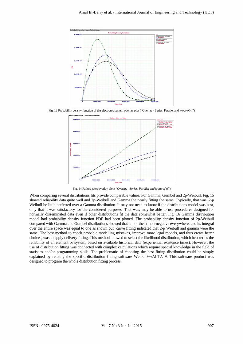
Fig. 13 Probability density function of the electronic system overlay plot (“Overlay - Series, Parallel and k‐out‐of‐n”)

Fig. 14 Failure rates overlay plot (“Overlay - Series, Parallel and k‐out‐of‐n”)

When comparing several distributions fits provide comparable values. For Gamma, Gumbel and 2p-Weibull. Fig. 15 showed reliability data quite well and 2p-Weibull and Gamma the nearly fitting the same. Typically, that was, 2-p Weibull be little preferred over a Gamma distribution. It may not need to know if the distributions model was best, only that it was satisfactory for the considered purposes. That was, may be able to use procedures designed for normally disseminated data even if other distributions fit the data somewhat better. Fig. 16 Gamma distribution model had probability density function PDF had been plotted. The probability density function of 2p-Weibull compared with Gamma and Gumbel distributions showed that all of them non-negative everywhere, and its integral over the entire space was equal to one as shown but curve fitting indicated that 2-p Weibull and gamma were the same. The best method to check probable modelling mistakes, improve more legal models, and thus create better choices, was to apply delivery fitting. This method allowed to select the likelihood distribution, which best terms the reliability of an element or system, based on available historical data (experiential existence times). However, the use of distribution fitting was connected with complex calculations which require special knowledge in the field of statistics and/or programming skills. The problematic of choosing the best fitting distribution could be simply explained by relating the specific distribution fitting software Weibull++/ALTA 9. This software product was designed to program the whole distribution fitting process.



Fig. 15Comparison Reliability (Gamma, Gumbel and 2p-Weibull).

Fig. 16 Comparison PDF (Gamma, Gumbel and 2p-Weibull).

Because higher reliability typically compared with higher production costs, lower warranty costs and higher market share. With Weibull++’s Target Reliability tool, visualization and estimation a target reliability that would minimize cost, maximize profit and/or maximize return on an investment in improving the product’s reliability. Fig. 17 indicated that reliability increases, production costs would increase, but the unreliability cost would decrease. The Cost vs. Reliability plot allowed to visualize the relationship between reliability and cost, as well as estimate the reliability that minimizes total cost (i.e., production cost + cost due to unreliability). The reliability that was estimated to minimize cost is 97.998% at the end of the warranty period. To maximize the return on investment, shown in Fig. 18 then the target reliability should be about 97.998% at the end of the warranty period (which is obviously very close to the 97.998% reliability needed to maximize cost). With this reliability for maximizing ROI, it could expected 2.002% of the units sold to be returned under warranty. Also noted that the profit increased directly proportional to the reliability until it reached the 97 998 % and then reliability improvement had been take money over than its benefits.



Fig. 17 Reliability Vs. Cost.

Fig. 18 ReliaSoft’s Reliability Return on Investment vs. Reliability

4. CONCLUSIONS

The simulation predicted (FEM) by using COMSOL Multiphysics to determine a maximum temperature of the silicon chip till to 95 °C which means that the device overheat. Also design failure modes for electronic devices systems. Weibull++standard folio had been used to estimate the warranty time which was near 153.48. By two-sided confidence bounds on the Weibull probability MTTF was estimated. The results of expected failure analysis indicated that first failure had been occurred sometime between 73 and 339 also the predicted failure time different than the actual failure and had been indicated it could be reduce the sample size. Degradation fit results the failure times of the units on test were extrapolated using measurements of their degradation over time. Second, once these failure times are obtained, life data analysis is used to estimate the reliability of the system. Analysis, the required test “time” with stress was estimated to predict the failure time. It concluded that if the chip was not cooling and the failure modes would be occurred and system temperatures must be viewed within the system or using a utility to monitor the chip settings. 2p-Weibull compared with Gamma and Gumbel distributions showed that all of them non-negative everywhere, and its integral over the entire space was equal to one as shown but curve fitting indicated that 2p- Weibull and gamma were the same. The best method to check probable modelling mistakes, improve more legal models, and thus create better choices, was to apply delivery fitting. The reliability that was estimated to minimize cost is 97.998% at the end of the warranty period to maximize the return on investment.

Acknowledgment

Authors would like to thank King Abdul-Aziz City for Science and Technology (KACST) for their kind supporting our research work.



References [1] Thomas M.Gruzs “A Survey of Neutral Currents in Three-phase Computer Power Systems” IEEE TRANSACTIONS ON INDUSTRY

APPLICATIONS, VOL. 26, NO. 4, JULYIAUGUST, pp. 719-725 1990. [2] V. M. DWYER,* A. J. FRANKLIN and D. S. CAMPBELL “THERMAL FAILURE IN SEMICONDUCTOR DEVICES” Solid state

electronics Vol. 33, No. 5, pp. 553-560, 1990 [3] Hong Xie, Mostafa Aghazadeh, Wendy Lui, and Kevin Haley “Thermal Solutions to Pentium Processors in TCP in Notebooks and Sub-

Notebooks” IEEE TRANSACTIONS ON COMPONENTS, PACKAGING, AND MANUFACTURING TECHNOLOGY-PART A, VOL. 19, NO. 1, MARCH 1996

[4] Vladimir Szekely, Marta Rencz and Bernard Courtois “Tracing the Thermal Behavior of ICs” IEEE DESIGN & TEST OF COMPUTERS, pp.14-21 and APRIL–JUNE 1998.

[5] S.Dilhaire, S. Jorez, A.Cornet, E. Schaub and W. Claeys “Optical method for the measurement of the thermo mechanical behavior of electronic devices” Microelectronics Reliability 39 pp.981-985, 1999.

[6] M. Gall, C. Capasso, D. Jawarani, R. Hernandez, and H. Kawasaki “Statistical analysis of early failures in electromigration” JOURNAL OF APPLIED PHYSICS, VOLUME 90, NUMBER 2, pp.732-740, 15 JULY 2001.

[7] John H. L. Pang, D. Y. R. Chong, and T. H. Low “Thermal Cycling Analysis of Flip-Chip Solder Joint Reliability” IEEE TRANSACTIONS ON COMPONENTS AND PACKAGING TECHNOLOGIES, VOL. 24, NO. 4, ,pp. 705-712, DECEMBER 2001.

[8] Chandrakant D. Patel, Ratnesh Sharma, Cullen E. Bash and Abdlmonem Beitelmal “Thermal Considerations in Cooling Large Scale High Compute Density Data Centers” 0-7803-7152-6/02/$10.00 Q 2002 IEEE, Inter Society Conference on Thermal Phenomena, pp.767- 776, 2002.

[9] Ching-Kong Chao, Shih-Yu Hung, and Cheng-Ching Yu “Thermal Stress Analysis for Rapid Thermal Processor” IEEE TRANSACTIONS ON SEMICONDUCTOR MANUFACTURING, VOL. 16, NO. 2, pp. 335- 341, MAY 2003.

[10] Ryan J. McGlen, Roshan Jachuck and Song Lin “Integrated thermal management techniques for high power electronic devices” R.J. McGlen et al. / Applied Thermal Engineering 24 pp.1143–1156, 2004.

[11] E.P. Zafiropoulos, E.N. Dialynas" Reliability and cost optimization of electronic devices considering the component failure rate uncertainty" Reliability Engineering and System Safety 84 pp.271–284, 2004.

[12] A. Sittithumwat, F. Soudi, K. Tomsovic," Optimal allocation of distribution maintenance resources with limited information" Electric Power Systems Research 68 pp.208–220, 2004.

[13] Jayanth Srinivasan, Sarita V. Adve, Pradip Bose, Jude A. Rivers “The Impact of Technology Scaling on Lifetime Reliability” Proceedings of the 2004 International Conference on Dependable Systems and Networks (DSN’04) 0-7695-2052-9/04, IEEE, 2004.

[14] Nikhil Vichare, Peter Rodgers, Valérie Eveloy, and Michael G. Pecht “In Situ Temperature Measurement of a Notebook Computer—A Case Study in Health and Usage Monitoring of Electronics” IEEE TRANSACTIONS ON DEVICE AND MATERIALS RELIABILITY, VOL. 4, NO. 4, pp. 658-663, DECEMBER 2004

[15] Weilin Qu and Issam Mudawar “Measurement and correlation of critical heat flux in two-phase micro-channel heat sinks” International Journal of Heat and Mass Transfer 47 pp. 2045–2059, 2004.

[16] Yan Qi, Hamid R. Ghorbani, and Jan K. Spelt “Thermal Fatigue of SnPb and SAC Resistor Joints: Analysis of Stress-Strain as a Function of Cycle Parameters” IEEE TRANSACTIONS ON ADVANCED PACKAGING, VOL. 29, NO. 4, NOVEMBER 2006

[17] Junwei Lu and Francis Dawson “EMC Computer Modeling Techniques for CPU Heat Sink Simulation” IEEE TRANSACTIONS ON MAGNETICS, VOL. 42, NO. 10, pp. 3171-3173 OCTOBER 2006.

[18] Joseph B. Bernstein *, Moshe Gurfinkel, Xiaojun Li, Jo¨rg Walters,Yoram Shapira, Michael Talmor "Electronic circuit reliability modeling" Microelectronics Reliability 46 pp. 1957–1979 ,2006.

[19] Bianca Schroeder and Garth A. Gibson “Understanding Failures in Petascale Computers” Journal of Physics: Conference Series 78, 012022, 2007.

[20] Srinivasan Murali, Almir Mutapcic, David Atienza, Rajesh Gupta, Stephen Boyd, and Giovanni De Micheli “Temperature-Aware Processor Frequency Assignment for MPSoCs Using Convex Optimization” CODES+ISSS’07, Salzburg, Austria. Copyright 2007 ACM 978-1-59593-824-4/07/0009 pp.111-116, September 30–October 3, 2007.

[21] Soon-Bok Lee and Ilho Kim" Reliability Assessment of Electronic Packaging with Hybrid Approach of Experimental and Computational Mechanics" APCOM’07 in conjunction with EPMESC XI, Kyoto, JAPAN , December 3-62007.

[22] M.A. Belaı¨d_, K. Ketata, K. Mourgues, M. Gares, M. Masmoudi, J. Marcon “Reliability study of power RF LDMOS device under thermal stress” Microelectronics Journal 38, pp.164–170, 2007.

[23] S. Pietranico, S. Pommier, S. Lefebvre and S. Pattofatto “Thermal fatigue and failure of electronic power device substrates” International Journal of Fatigue 31 ,pp. 1911–1920, 2009.

[24] Hyung Beom Jang, Ikroh Yoon, Cheol Hong Kim, Seungwon Shin, and Sung Woo Chung “The Impact of Liquid Cooling on 3D Multi-Core Processors” IEEE. 978-1-pp.4244-5028,2009.

[25] M. Diatta , E. Bouyssou, D. Trémouilles, P. Martinez, F. Roqueta, O. Ory, M. Bafleur" Failur mechanisms of discrete protection device subjected to repetitive electrostatic discharges (ESD)" Microelectronics Reliability 49,pp. 1103–1106, 2009 .

[26] Y. Q. Ni, M.ASCE; X. W. Ye; and J. M. Ko, F.ASCE “Monitoring-Based Fatigue Reliability Assessment of Steel Bridges: Analytical Model and Application” JOURNAL OF STRUCTURAL ENGINEERING © ASCE /,pp 1563- 1573, DECEMBER 2010.

[27] J. Virkki, A. Koskenkorva, L. Frisk "Development of a matrix test board for capacitor reliability testing “Microelectronics Reliability 50 pp.1711–1714, 2010.

[28] F. Hedrich∗, K. Kliche, M. Storz, S. Billat, M. Ashauer, R. Zengerle " Thermal flow sensors for MEMS spirometric devices Sensors and Actuators A 162 pp. 373–378 , 2010.

[29] T. Abbas, K. M. Abd_elsalam, and KH. Khodairy “CPU thermal management of Personal and notebook computer (Transient study)” Thermal Issues in Emerging Technologies, ThETA 3, Cairo, Egypt, pp.85-93, Dec 19-22nd 2010.

[30] Tsunaki Takahashi, Nobuyasu Beppu, Kunro Chen, Shunri Oda, and Ken Uchida “Thermal-Aware Device Design of Nanoscale Bulk/SOI FinFETs: Suppression of Operation Temperature and Its Variability” IEDM11, IEEE, pp. 34.6.1- 34.6.4, 2011.

[31] Zheming Zhang, Jingshen Wu “Research on Temperature Gradient Effect to Solder Joint Reliability” 978-1-4673-4944-4©IEEE ,2012. [32] Larisa Mariut “Temp erature Gradient Effect on Partial Discharge Activity-Modelling and Simulation” 978-1-4673-1810-5/12/$31.00,

IEEE, 2012. [33] M.-N. Sabry and M. Dessouky, “A framework theory for dynamic compact thermal models,” in Proc. 28th Annu. IEEE Semicond.

Thermal Meas. Manag. Symp. (SEMI- THERM), pp. 189–194., Mar. 2012. [34] Chuan Xu, Member, Seshadri K. Kolluri, Member, Kazhuhiko Endo, Member, and Kaustav Banerjee “Analytical Thermal Model for Self-

Heating in Advanced FinFET Devices With Implications for Design and Reliability” IEEE TRANSACTIONS ON COMPUTER-AIDED DESIGN OF INTEGRATED CIRCUITS AND SYSTEMS, VOL. 32, NO. 7, pp. 1045-1058, JULY 2013.

[35] Huaiyu Ye, Xianping Chen, Henk van Zeijl, Alexander W. J. Gielen, and Guoqi Zhang “Thermal Transient Effect and Improved Junction Temperature Measurement Method in High-Voltage Light-Emitting Diodes” IEEE ELECTRON DEVICE LETTERS, VOL. 34, NO.



9,.pp.1178174, SEPTEMBER 2013. [36] Dragica Vasileska “Modeling thermal effects in nano-devices” Microelectronic Engineering 109 pp.163–167, 2013. [37] Wangkun Jia, Brian T. Helenbrook, and Ming-Cheng Cheng “Thermal Modeling of Multi-Fin Field Effect Transistor Structure Using

Proper Orthogonal Decomposition” IEEE TRANSACTIONS ON ELECTRON DEVICES, VOL. 61, NO. 8, pp. 2752-2759, AUGUST 2014.

[38] Henry Wong and Tien-Yu Tom Lee “Thermal Evaluation of a PowerPC 620 Multi-Processor Computer” 0-7803-3139-7/96/$4.010 09 IEEE, Twelfth IEEE SEMI-THERMTM symposiumPp.73-80,1996.

[39] V. M. DWYER,* A. J. FRANKLIN and D. S. CAMPBELL “THERMAL FAILURE IN SEMICONDUCTOR DEVICES” Solid state electronics Vol. 33, No. 5, pp. 553-560, 1990

[40] Mitchell 0. Locks “How To Estimate the Parameters of a Weibull Distribution” Quality Progress 35 no8, pp58-64, Ag 2002. [41] Necip Doganaksoy, Gerald J. Hahn and William Q. Meeker “Reliability Analysis By Failure Mode” Quality Progress 35 no6 ,Je 2002 [42] Jayanth Srinivasan, Sarita V. Adve, Pradip Bose and Jude A. Rivers “The Case for Lifetime Reliability-Aware Microprocessors”

Proceedings of the 31st Annual International Symposium on Computer Architecture (ISCA’04) IEEE 1063-6897/04 $ 20.00 , 2004. [43] G. Cassanelli,*, G.Mura, F.Cesaretti, M.Vanzi, F.Fantini"Reliability predictions in electronic Industrial applications" Microelectronics

Reliability 45 pp.1321–1326, 2005. [44] Y.A. Chau and K.Y.-T. Huang “Correlated multivariate Weibull fading channels with selection diversity” ELECTRONICS LETTERS,

Vol. 43 No. 3, 1st February 2007. [45] Srinivasan Murali, Almir Mutapcic, David Atienza, Rajesh Gupta, Stephen Boyd, and Giovanni De Micheli “Temperature-Aware

Processor Frequency Assignment for MPSoCs Using Convex Optimization” CODES+ISSS’07, Salzburg, Austria. Copyright 2007 ACM 978-1-59593-824-4/07/0009 ...$5.00.pp.111-116 ,September 30–October 3, 2007.

[46] Sharmila Banerjee and Boris Iglewicz “A Simple Univariate Outlier Identification Procedure Designed for Large Samples” Communications in Statistics—Simulation and Computation®, 36:, Copyright © Taylor & Francis Group, LLC ISSN: 0361-0918 print/1532-4141 online DOI: 10.1080/03610910601161264, pp.249–263 2007

[47] D.W. Matolak I. Sen W. Xiong “Generation of multivariate Weibull random variates” IET Commun., Vol. 2, No. 4, pp. 523–527,2008. [48] Tongdab Jin and Lakshmana Gonigunta “Weibull and Gamma Renewal Approximation Using Generalized Exponential Functions

"Communications in Statistics—Simulation and Computation®, 38:, Copyright © Taylor & Francis Group, LL ISSN: 0361-0918 print/1532-4141 online DOI: 10.1080/03610910802440327, 154–171, 2009.

[49] K.S. Sultan, M.A. Ismail and A.S. Al-Moisheer “Testing the number of components of the mixture of two inverse Weibull distributions” International Journal of Computer Mathematics Vol. 86, No. 4, pp. 693–702, April 2009.

[50] Anduin E. Touw "Bayesian estimation of mixed Weibull distributions" Reliability Engineering and System Safety 94 pp.463– 473,2009. [51] Govind S. Mudholkara, Kobby O. Asubonteng, Alan D. Hutson," Transformation of the bathtub failure rate data in reliability for using

Weibull-model analysis "Statistical Methodology 6 pp.622:633 ,2009. [52] S. M. K. Quadri and N. Ahmad “Software Reliability Growth Modeling with New Modified Weibull Testing–effort and Optimal Release

Policy” International Journal of Computer Applications (0975 – 8887)Volume 6– No.12, September 2010. [53] Kahadawala Cooray, Sumith Gunasekera and Malwane Ananda “Weibull and inverse Weibull composite distribution for modeling

reliability data” Model Assisted Statistics and Applications 5 pp.109–115, 2010. [54] LAURA J. FREEMAN and G. GEOFFREY VINING “Reliability Data Analysis for Life Test Experiments with Subsampling” Journal of

Quality Technology, VoL 42, No. 3, pp. 233- 241, July 2010. [55] B. hari prasad, P. bhattacharjee and A. venugopal “Prediction of Vehicle Reliability using ANN” International Journal of Perform ability

Engineering, Vol.8, No.3, pp. 321-329, May 2012.



Documents

Reliability Models to Predict Engineering Systems ... · Reliability Models to Predict Engineering Systems 'Failures and Improve their Performance Amal El-Berry 1, and Afrah Al-Bossly2