This work is licensed under a Creative Commons Attribution-NonCommercial-ShareAlike License. Your use of this material constitutes acceptance of that license and the conditions of use of materials on this site.

Copyright 2006, The Johns Hopkins University and Jeannie-Marie Leoutsakos. All rights reserved. Use of these materials permitted only in accordance with license rights granted. Materials provided “AS IS”; no representations or warranties provided. User assumes all responsibility for use, and all liability related thereto, and must independently review all materials for accuracy and efficacy. May contain materials owned by others. User is responsible for obtaining permissions for use from third parties as needed.

Statistics in Psychosocial ResearchLecture 4

Reliability II

Lecturer: Jeannie-Marie Leoutsakos

Outline

• Review of ANOVA• Intra-Class Correlations• Reliability Examples• Other Research Designs

-30

36

912

15sc

ore

1 2 3group

Are the true means for each group different from each other?

-80

-60

-40

-20

020

4060

8010

0sc

ore1

1 2 3group

Compare amounts of variance within & between groups

i=1…,I indexes groups, j=1,…ni indexes members of group

Source of Variation

DF Sum of Squares (SS)

Mean Square (MS)

F-Ratio

BetweenGroup

WithinGroup

1−I

IN −

∑ − 2)( YYn ii

∑∑ −i j iij YY 2)(

DFSSBMSB =

DFSSWMSW =

MSWMSB

. oneway score1 group

Analysis of VarianceSource SS df MS F Prob > F

------------------------------------------------------------------------Between groups 4054.76741 2 2027.38371 2030.92 0.0000Within groups 1494.39042 1497 .998256793------------------------------------------------------------------------

Total 5549.15783 1499 3.70190649

-80

-60

-40

-20

020

4060

8010

0

1 2 3group

score1 score2

. oneway score13 group

Analysis of Variance

Source SS df MS F Prob > F

------------------------------------------------------------------------

Between groups 4145.64545 2 2072.82273 2.42 0.0891

Within groups 1281245.47 1497 855.8754

------------------------------------------------------------------------

Total 1285391.12 1499 857.499079

Intraclass correlation: Assessing inter-rater reliability

• As before, reliability defined as:variance in true scores ⁄ variance in observed scores

• For the intra-class correlation the specific form of this equation can take on at least six different forms

• The correct form to use depends on the study design and the researcher’s assumptions about the patients and subjects (or items)

• I will discuss three designs, each with two ICCs

Overview• Unique Design: Each of the I subjects rated by a unique

set of m raters (m>1), such that the total number of raters, R, is m*I

• Fixed Design: Each subject is rated by each of the same m raters, such that the total number of raters, R is m. These raters are the only raters of interest.

• Random Design: m raters are drawn from a larger pool of raters. Each of the I subjects is rated by each of the m raters. Again, the total number of raters, R is m.

NOTE: raters might be people or questionnaire items

Unique Design

• No Overlap of Raters

rater1 rater2 rater3 rater4 rater5 rater6

s1 s2 s3

• m=2, I=3 # of raters=m*I=6

Fixed Design

• Total Overlap of Raters

s1 s2 s3

rater1 rater3rater2

• m=3, n=3 # of raters=m=3

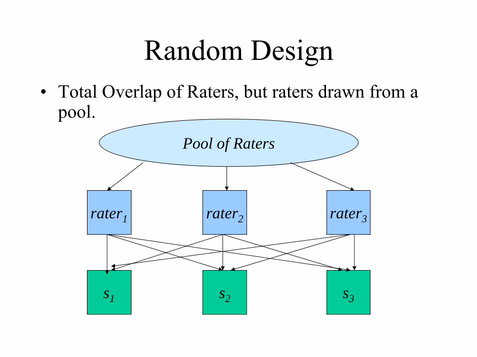
Random Design• Total Overlap of Raters, but raters drawn from a

pool.

s1 s2 s3

rater1 rater3rater2

Pool of Raters

Types of Reliability

• There are two (at least) types of reliability associated with each of these designs.– Reliability of mean ratings: reliability of

average of all ratings per subject– Reliability of one individual rating: reliability

of a single rating of one subject• Which will be higher? • Why?

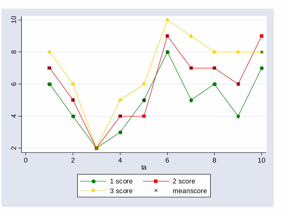
24

68

10

0 2 4 6 8 10ta

1 score 2 score3 score meanscore

Unique Rater Design ICC

Equation to estimate reliability of rating means

Between Mean Square Variance – Within Mean Square Variance

Between Mean Square Variance

MSB – MSWMSB

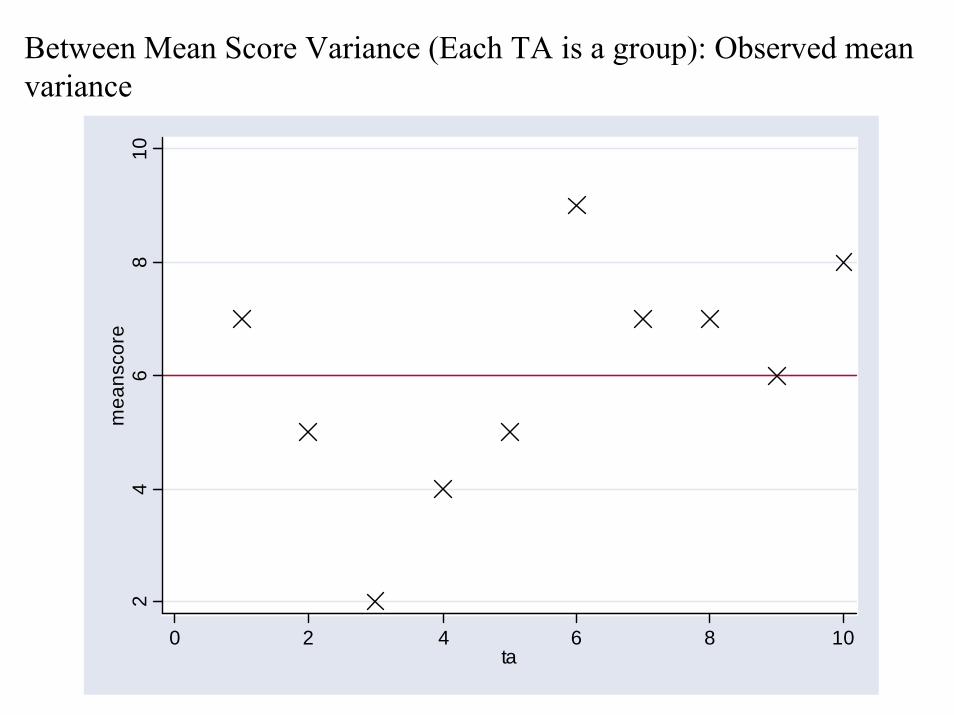
Between Mean Score Variance (Each TA is a group): Observed mean variance

24

68

10m

eans

core

0 2 4 6 8 10ta

Between Mean Score VarianceDegree to which mean score of rated subjects differ from grand mean

( ) ( ) 22

1

2

11

b

I

iib YYm

Is σ≅−

−= ∑

=

• I = number of people being rated (# of TAs)• = mean score for each TA rated• = overall mean of scores for whole sample• m = number of raters for each mean

iYY

Unique Rater Design1) Between Mean Score Variance, steps in Stata

a) calculate mean scores for each individual*e.g. egen meanta = rmean(score1 score2 score3)

b) calculate overall mean*e.g. egen grandmean = mean(meanta)

c) calculate deviation of individual mean from group mean*e.g. gen bsquarei = 3*(meanta-grandmean)^2

d) add up all deviations in (c)*e.g. egen bsquare = sum(bsquarei)

e) divide sum of squares by degrees of freedom*e.g. display bsquare/(10-1) =

Unique Rater Design (cont’d)2) Within Mean Score Variance: Degree to which individual

scores differ from a subject’s mean score

( ) ( ) 22

11

2

11

w

m

jiij

I

iw YY

mIs σ≅−

−= ∑∑

==

Where:• I = number of individuals being rated (# of TAs)• R = number of raters• Yij = score of each individual rater • = mean score of each person rated • m = number of raters for each meanNote: R=m

iY

Unique Rater Design3) Within Mean Score Variance, steps in Stata

a) calculate mean scores for each individual*e.g. egen meanid = rmean(score1 score2 score3)

b) calculate deviation of rater from individual mean*e.g. gen wsquarei = (score1-meanid)^2 + (score2-meanid)^2

+ (score3- meanid)^2c) add up deviations in (b) across all individuals

*e.g. egen wsquare =sum(wsquarei)d) divide sum of squares by degrees of freedom

*e.g. display wsquare/I*(m-1) =

Unique Rater DesignShortcut: Use procedure ‘oneway’ in Stata

First, must “reshape” data.

. reshape long score, i(ta) j(rater)

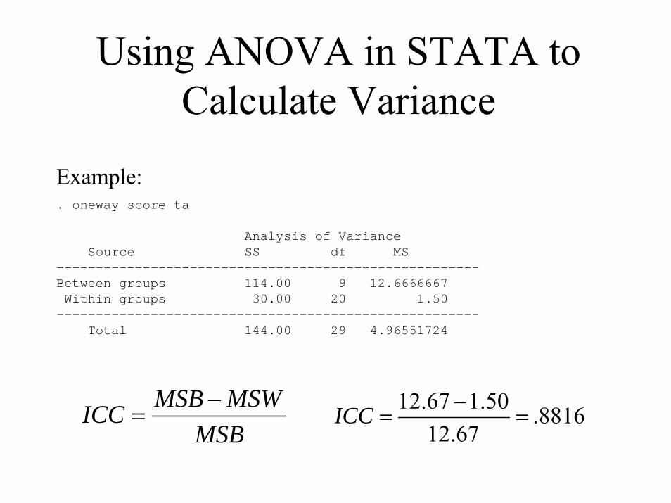
Using ANOVA in STATA to Calculate Variance

Example:. oneway score ta

Analysis of VarianceSource SS df MS

------------------------------------------------------Between groups 114.00 9 12.6666667Within groups 30.00 20 1.50

------------------------------------------------------Total 144.00 29 4.96551724

MSBMSWMSBICC −

= 8816.67.12

50.167.12=

−=ICC

Important Note

1. Reliability is a group-specific statistic.

2. The greater the variance in the true scores of a population, thehigher the reliability of the measure (if observed variance is constant)

Variance in true scoresReliability =

Variance in observed scores

Reliability for Individual Ratings

So far we’ve calculated reliability of the mean score for each TA.

What is the average reliability of each individual rating of the TA?

Reliability of Individual Scores in Unique Rater Design

MSWmMSBMSWMSB

)1( −+−

Where m = number of raters per TA

Continuing with our example:

7128.50.1*)13(67.12

)50.167.12(Re =−+−

=liability

Fixed Rater Design1) Each subject rated by each of the same m raters, who are the only raters of interest

2) examples:

3) Computation involves two-way analysis of variance

4) Before: two sources of error, (differences across individuals, and error inherent to the measurement) Error now only has one source: error due to individuals is ‘controlled.’

Fixed Rater DesignRecall that the equation for Unique Rater Design was:

MSB – MSWMSB

Which can also be expressed as:

MSB– (MSRater + MSE)MSB

The equation for the fixed rater design is very similar:

MSB– (MSE)MSB

24

68

10

0 2 4 6 8 10ta

1 score 2 score3 score meanscore

Rater Mean Variance5

5.5

66.

57

1 1.5 2 2.5 3rater

mean1 mean2mean3

Fixed Rater DesignRater Mean Score Variance: Degree to which raters’mean scores differ from those of the overall mean

( ) ( ) ( ) 22

1

2

11

r

m

jjr YYI

ms σ≅−

−= ∑

=

Where:

• m = number of raters (in fixed design, R=m)• I = number of subjects evaluated (# of TAs)• = mean score of rater• = overall mean score for sample Y

jY

Fixed Rater DesignSteps in Stata1. Calculate overall mean2. Calculate mean for each rater

*e.g. egen r1mean=mean(rater1)egen r2mean=mean(rater2)…

3. Calculate deviation of rater mean from overall mean

*e.g. display N*(r1mean-grandmean)^2 +N*(r2mean-grandmean)^2…

4. Calculate error square variance*error square variance = (within square variance – rater

square variance)*divide by difference in degrees of freedom to get

error variance

Using ANOVA in STATA to Calculate Variance

Example:. anova score ta Rater

Source | Partial SS df MS ---------+--------------------------------Model | 134.00 11 12.1818182 ta | 114.00 9 12.6666667 Rater | 20.00 2 10.00 Residual | 10.00 18 .555555556 -----------+------------------------------Total | 144.00 29 4.96551724

ICC for Fixed Rater Design, Group mean =

96.67.12

56.67.12=

−=

−MSB

MSEMSB

Fixed Rater Design

Equation to estimate reliability for individual rater’s scores:

MSB– MSEMSB + (m-1)*MSE

Where R = m = number of raters

Final Estimate:

12.67 - .56 = .878212.67 + (2)(.56)

Random Rater Design1. Randomly-selected raters evaluate each subject

2. Computation involves two-way analysis of variance

3. Error has two sources again, but error due to individual raters is reduced

4. Deciding between Random and Fixed design:

Would you wish to generalize findings from this sample to situations with a different set of raters? If so, you would use the random rater design.

Random Rater Design: Reliability for Mean Score of Each Subject

)/)(( IMSEMSRaterMSBMSEMSB−+

−

Source | Partial SS df MS

---------+--------------------------------

Model | 134.00 11 12.1818182

ta | 114.00 9 12.6666667

Rater | 20.00 2 10.00

Residual | 10.00 18 .555555556

-----------+------------------------------

Total | 144.00 29 4.96551724

2) Take into account error for rater bias

3) ICC = 12.67 – 0.56 = .8912.67 + (10 – 0.56)/10

Random Rater Design: Reliability for Individual Score

Source | Partial SS df MS

---------+--------------------------------

Model | 134.00 11 12.1818182

ta | 114.00 9 12.6666667

Rater | 20.00 2 10.00

Residual | 10.00 18 .555555556

-----------+------------------------------

Total | 144.00 29 4.96551724

IMSEMSRatermMSEmMSBMSEMSB

/)(**)1( −+−+−

12.67 – 0.56ICC =

12.67 +( 2*.56) + 3*(10.0 – .56)/10= .72

Summary1. Unique Rater Design: Each subject rated by a different set of m

raters; formulas use between and within mean square variance

2. Fixed Rater Design: Each target is rated by each of the same mraters, who are the only raters of interest; formulas use between and error square variance

3. Random Rater Design: m raters, in (2), were drawn from a random sample of raters; formula uses between and error square variance, adjusting for rater variance

Which ICC Is Most Appropriate?Scenario 1: A target child’s three best friends all report on the

target child’s level of drug use.

Scenario 2: You develop a screener to help identify victims of domestic abuse in emergency rooms; each patient is to be rated by three nurses at each hospital and you use the mean score in your analyses.

a) Which ICC would give you the estimated reliability for the nurses at your one pilot hospital?

b) Which ICC would give you an estimate of the reliability for the measure when used by different nurses at different hospitals?

c) Which ICC would give you an estimate for the reliability of the measure if it were to be administered by only one nurse instead of three?

Question 1

State the conditions under which the Unique Rater ICC (for mean values of an item) is identical to the value of the Fixed Rater ICC (for mean values of an item)?

Answer in terms of the variance of between, within, and rater sum of squares.

Solution 1

Question 2You have developed a new survey measure of bipolar disorder on the basis of a pilot population composed of one third with severe symptoms, one third with mild symptoms, and one third without any symptoms. It turns out that your measure has a high reliability of .90. You find funding and administer your survey to a nationally representative sample, only to find that your reliability is now much lower.

What might be the explanation ?

Solution 2

pilot

pilot

MSBMSWMSB −

=90.

There is inherent assumption here that the national sample will have the same makeup with regard to severity. If that’s not so, then the reliability may drop because the between-person variance in the national sample was lower than it was in the pilot sample, while the within-person variance was presumably about the same.

Question 3

Doesn’t high reliability imply that two measures of the same characteristic will yield the same answer? If so, why do I see graphs that imply higher reliability when sample variability is higher?

It is important to keep in mind that there are two types of variance: within-person variance and between-person variance. It is correct that when the within-person variance is high a measure typically will have low reliability. The within-person variance is a measure of the error variance, and the higher the error variance of a measure the lower its reliability. With high levels of within-person variance, measures of the same characteristic on multiple occasions will lead to different answers.

In contrast, high levels of between-person variance help improve the reliability of a measure. The more between-person variance in a population, the greater the proportion of variance that is due to the true underlying characteristic in proportion to the variance due to error, and the greater the overall reliability.

Solution 3

Question 4

Imagine two graphs, Figure 1 and Figure 2, in which all respondents have the same mean score. If Figure 2 shows a wider spread in individual means than is shown in Figure 1, which of the two graphs has the higher reliability.

Solution 4

Figure 1 has the higher reliability. The between-person variance in both graphs is the same (all respondents have the same mean score). The within-person variance is higher in Figure 2 than it is in Figure 1 (indicated by a wider spread across the individual means). Therefore, Figure 1 has higher reliability.

Question 5

Using observed score as the y axis and true score as the x axis, draw a measure with a negative covariance between true score and error term.

-20

-10

010

20O

bser

ved

Scor

e (N

egat

ive

Cor

rela

tion)

0 2 4 6 8 10True Score

Solution 5

Question 6

Using observed score as the y axis and true score as the x axis, draw a measure with a positive covariance between true score and error term.

-10

010

2030

Obs

erve

d Sc

ore

(Pos

itive

Cor

rela

tion)

0 2 4 6 8 10True Score

Solution 6

Question 7Scenario 1: Reported correlation between years of educational attainment and adults’ scores on an anti-social personality (ASP) disorder scale is about .30; reported reliability of the education scale is about .95; reported reliability for the ASP scale it is about .70.

Scenario 2: Reported reliability of the education scale is the same (.95); reported reliability of the ASP disorder scale is now .40.

What is the observed correlation between the two measures in Scenario 2?

Solution 7

367883.70.95.

30.=

×==

yyxx

xyTxTy rr

rr

solve for rxy

227.40.*95.367883. =×=×= yyxxTxTyxy rrrr

Question 8

A. How are the alpha and the split-half reliability coefficient conceptually related?

B. For mean scores, how are the alpha and the Fixed Rater ICC related?

Solution 8

A. Cronbach’s alpha is the average of all possible split-half reliabilities.

B. Cronbach’s alpha is mathematically equivalent to the Fixed Rater ICC for mean scores.

Question 9

For a ten-item scale with an average inter-item correlation of .25, the reliability is .75. What about a twenty-item scale with the same average inter-item correlation? How about fifteen items? How about 5?

Solution 9Use Spearman-Brown Prophesy Formula

Reliability New Scale = N(R)/(1+(N-1)R) N = (number of desired items)/(number of items in observed scale)R = reliability of observed scale

For 20 item scale: R = (2*.75)/(1+.75) = .86For 15 item scale: R = (1.5*.75)/(1+.5*.75) = .82For 5 item scale: R= (.5*.75)/(1-.5*.75) = .60

Question 10Two psychiatrists disagree when rating a dichotomous child health outcome among 100 children. In ten of the cases, Dr. Green ratedthe outcome as present when Dr. Brown rated it as absent. In another ten cases, the reverse occurred; Dr. Brown rated the outcome as present while Dr. Green rated it as absent.

If both Dr. Green and Dr. Brown agree that fifty children have the outcome, what will be the value of the Kappa coefficient?

If they agree that 70 children have the outcome, will the Kappa be higher or lower?

Solution 10+ -

+ 50 10 60

- 10 30 40

60 40 100

+ -

+ 60*60/100=36 60*40/100=24 60

- 60*40/100=24 40*40/100=16 40

60 40 100

Question 11

Measures of self-reported discrimination sometimes violate the assumptions of classical test theory. Please provide a substantive example of violation for each of the three assumptions.

Solution 11E(x) = 0 could be violated if the true score is underreported as a result of social desirability bias

Cov(Tx,e)= 0 could be violated if people systematically overreported or underreported discrimination at either high or low extremes of the measure

Cov(ei,ej)= 0 could be violated if discrimination was clustered within certain areas of a location, and multiple locations were included in the analysis pool.

Question 12

An 10-item ASP measure with a reliability of .6 and an HIV risk-behavior measure with a reliability of .5 correlate at .30. How many additional items with similar item-level reliability must be added to the ASP measure to make the observed correlation ≥.35?

Solution 12

1. Solve for true correlation

2. The true correlation is constant;

therefore, rxx (and/or ryy) must

get bigger to raise the observed

correlation.

Solution 12 (cont’d)

3. Determine how many items to add

by using Spearman-Brown

prophesy formula.

4. Solve for N

Solution: The ASP scale must have ≥12 items for an expected observed correlation with HIV risk-behavior of .35 or greater.

Other Research Designs

• We saw, with the fixed ICC, how we could partition the variance, and reduce MSE

Fixed Effects(a) Set by experimenter (eg, treatment in an

RCT)(b) it is unreasonable to generalize beyond

conditions. (eg, reading ability as a function of grade in school)

(c) when the # of possibilities is small, and all are included in the study design (eg, sex, in a study with both males and females)

Random Effects

(a) Multiple possible values (eg, personality measures, age).

(b) Study subjects are considered a representative sample from a larger population.

(c) Experimenter wishes to generalize the results of the study beyond the study sample.

• We already saw an example of this with the fixed and random ICC’s.

• Part of a larger group of study designs under the heading of “generalizabilitytheory” popularized by Cronbach, and others.

• Can take 140.655 (LDA) and/or 140.656 (Multilevel models)