Embed Size (px)
Citation preview
Draft
Reliability-Based Geotechnical Design in the 2014 Canadian
Highway Bridge Design Code
Journal: Canadian Geotechnical Journal
Manuscript ID cgj-2015-0158.R1
Manuscript Type: Article
Date Submitted by the Author: 30-Jun-2015
Complete List of Authors: Fenton, Gordon; Dalhousie University, Dept. of Engineering Mathematics Naghibi, Farzaneh; Dalhousie University, Engineering Mathematics Dundas, David; Peto-MacCallum Ltd, Bathurst, Richard; Queens University/Royal Military College, Griffiths, D.; Colorado School of Mines, Civil and Environmental Engineering
Keyword: geotechnical code development, reliability-based geotechnical design, load and resistance factor design, Canadian design codes, design code comparison
https://mc06.manuscriptcentral.com/cgj-pubs
Canadian Geotechnical Journal
Draft
1
Reliability-Based Geotechnical Design
in the 2014 Canadian Highway Bridge Design Code
by Gordon A. Fenton1,2
, Farzaneh Naghibi3, David Dundas
4,Richard J. Bathurst
5, and D. V.
Griffiths6,7
Reviewer’s Version with Figures in-line
revised for the Canadian Geotechnical Journal, Jun 28, 2015
Abstract
Canada has two national civil codes of practice that include geotechnical design provisions:
the National Building Code of Canada and the Canadian Highway Bridge Design Code. For
structural designs, both of these codes have been employing a Load and Resistance Factor format
embedded within a Limit States Design framework since the mid-1970’s. Unfortunately, Limit
States Design in geotechnical engineering has been lagging well behind that in structural
engineering for the simple fact that the ground is by far the most variable (and hence uncertain) of
engineering materials. Although the first implementation of a geotechnical limit states design
code appeared in Denmark in 1956, it was not until 1979 that the concept began to appear in
Canadian design codes, i.e., in the Ontario Highway Bridge Design Code which later became the
Canadian Highway Bridge Design Code (CHBDC). The geotechnical design provisions in the
CHBDC have evolved significantly since their inception in 1979. This paper describes the latest
1 Professor, Engineering Mathematics Dept., Dalhousie University, Halifax, Nova Scotia, Canada B3J 2X4.
(Corresponding Author) [email protected] 2 Faculty of Civil Engineering and Geosciences, Delft University of Technology, Delft, The Netherlands
3 Post-doctoral researcher, Engineering Mathematics Dept., Dalhousie University, Halifax, Nova Scotia, Canada
B3J 2X4, [email protected] 4 Professional Engineer, former Senior Foundations Engineer, Ontario Ministry of Transportation. [email protected]
5 Professor, Civil Engineering Dept., Royal Military College of Canada, Kingston, Ontario, Canada K7K 7B4.
[email protected] 6 Professor, Division of Engineering, Colorado School of Mines, Golden, Colorado 80401-1887, USA.
[email protected] (F.ASCE) 7 Australian Research Council Centre of Excellence for Geotechnical Science and Engineering, University of
Newcastle, Callaghan NSW 2308, Australia
Page 1 of 63
https://mc06.manuscriptcentral.com/cgj-pubs
Canadian Geotechnical Journal
Draft
2
advances appearing in the CHBDC along with the steps taken to calibrate its recent geotechnical
resistance and consequence factors.
Keywords: geotechnical code development, reliability-based geotechnical design, load and
resistance factor design, Canadian codes, code comparison
1. Introduction
Worldwide, geotechnical design codes have been migrating towards reliability-based design
concepts for several decades now. For example, the ISO 2394 (International Organization for
Standardization , 2015), which provides general principles of reliability for structures, now contains
an Annex D entitled “Reliability of geotechnical structures”. However, prior to 1979, geotechnical
design in Canada was based on the classic working stress design (WSD) format which involved
satisfying an equation of the form
ˆ ˆs i
i
R F F≥ ∑ (1)
where R is the characteristic (also known as nominal or design) resistance, sF is a factor of safety,
and ˆiF is the thi characteristic (nominal or design) load effect. The factor of safety was traditionally
used to account for all sources of uncertainty and is often defined as the ratio of the mean
resistance to the mean load. Unfortunately, this definition does not take the width of the resistance
and load distributions into account and, thus, the factor of safety cannot accurately reflect the
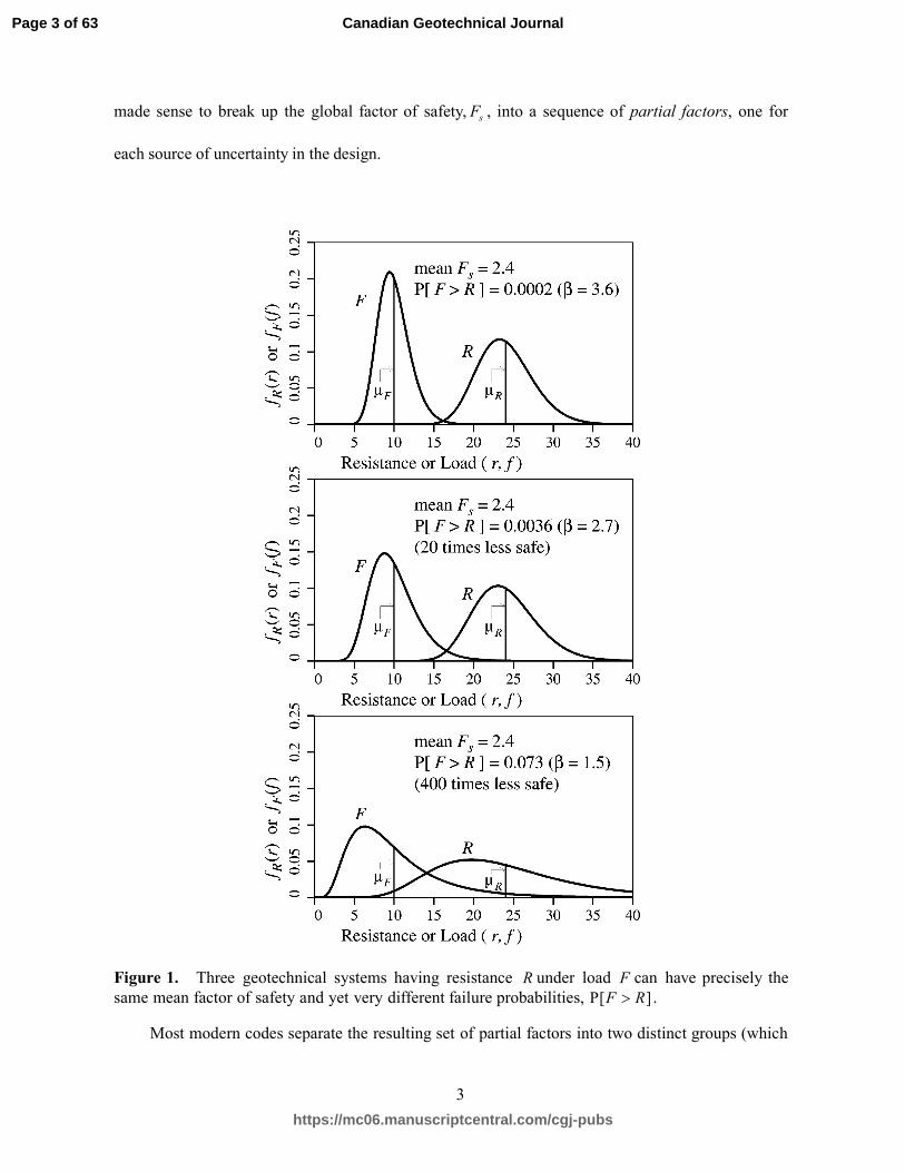
probability of failure of the geotechnical system. Figure 1 illustrates the classic problem with the
factor of safety. Although all three plots have the same mean factor of safety ( 2.4sF = ), the top plot
represents a system which is 400 times safer than the bottom plot, in terms of failure probability.
In recent decades, it has been recognized that not all sources of uncertainty are equal. For
example, live loads are usually less certain than dead loads, concrete strengths less certain than
steel strengths, and soil strengths less certain than most other engineering properties. It has thus
Page 2 of 63
https://mc06.manuscriptcentral.com/cgj-pubs
Canadian Geotechnical Journal
Draft
3
made sense to break up the global factor of safety, sF , into a sequence of partial factors, one for
each source of uncertainty in the design.
Figure 1. Three geotechnical systems having resistance R under load F can have precisely the
same mean factor of safety and yet very different failure probabilities, P[ ]F R> .
Most modern codes separate the resulting set of partial factors into two distinct groups (which
Page 3 of 63
https://mc06.manuscriptcentral.com/cgj-pubs
Canadian Geotechnical Journal
Draft
4
are nevertheless inversely related): the load factors and the resistance factors. These two groups of
factors lead to a design methodology referred to as Load and Resistance Factor Design (LRFD). The
partial factors are individually related to the variability of the quantity that they are factoring and are
used to scale the characteristic design values to more conservative values such that the overall
probability of system failure is acceptably small. In general, this means that loads are scaled up
(so long as they are acting in a way that reduces overall system safety) and resistances are scaled down
so that the final factored design values are acceptably conservative. Under the LRFD approach,
designs must satisfy an equation of the following form (although the right hand side is often
expressed more precisely as a series of possible load combinations),
ˆ ˆg i i i i
i
R I Fϕ ηα≥∑ (2)
where gϕ is a geotechnical resistance factor, R is the characteristic geotechnical resistance (based
on characteristic ground parameters), and, for the thi characteristic load effect ( ˆiF ), iI is a structure
importance factor, iη is a load combination factor, and
iα is the load factor.
In this paper, the word characteristic is used because it suggests a value that characterizes (in
some sense) a design parameter that is uncertain, e.g., a random load or resistance. The commonly
used words nominal or design do not convey the underlying randomness of the design parameter,
and so will not be used here. Some design codes (e.g., the Eurocodes) provide a specific statistical
definition of the word characteristic, often as being the 5th or 95th percentile, whichever leads to
the highest probability of failure. Eurocode 7 (CEN, 2004) provides a slightly different definition of a
characteristic parameter, in geotechnical design, as the value selected such that the probability of
occurrence of the associated limit state does not exceed 5%. The Eurocode 7 definition is discussed
in more detail in the Section entitled “Characteristic Resistance and Bias Factors”. Most other
geotechnical design codes provide only vague definitions for the characteristic value. For example,
one popular definition is “a conservative estimate of the mean.”
Page 4 of 63
https://mc06.manuscriptcentral.com/cgj-pubs
Canadian Geotechnical Journal
Draft
5
In most modern civil design codes, and Canada is no exception, the LRFD approach is
embedded within a Limit States Design (LSD) framework, where the LRFD formulation is satisfied
for each of a sequence of possible failure modes, or limit states. Generally, the load and resistance
factors are specifically selected for the limit state under consideration. For example, designing against
the limit state of bearing capacity failure would usually involve different factors than designing against
the limit state of excessive settlement.
The load and resistance factor method typically appears in one of two forms in geotechnical
design codes around the world;
1) the partial resistance factor approach, in which the individual components of ground strength,
e.g. cohesion and friction, are factored separately. The rationale behind this approach is that
the components of strength have different levels of uncertainty – for example, cohesion is
generally deemed to be more uncertain than friction angle. This is analogous to how live and
dead loads are factored separately.
2) the total resistance factor approach, in which the geotechnical resistance is computed in the
traditional way using best estimates of the ground parameters (i.e. characteristic values) and
then the final result is factored. This approach is more analogous to how resistances are
factored in structural engineering where each engineering material (e.g. concrete, steel, and
wood) has its own resistance factor. The ground is then viewed as just another engineering
material. The total resistance factor approach, commonly referred to as LRFD in North
America, also allows for very simple calibration to traditional working, or allowable, stress
design in that the factor of safety is just equal to the ratio of the load to resistance factors (see,
e.g., Honjo et al., 2009).
In 1979 and then again in 1983 the Ontario Highway Bridge Design Code (OHBDC) adopted the
partial resistance factor approach from Danish practice, in which components of ground strength
(e.g., cohesion and friction angle) were individually factored. In 1983, the LSD approach became
Page 5 of 63
https://mc06.manuscriptcentral.com/cgj-pubs
Canadian Geotechnical Journal
Draft
6
mandatory in the Ontario bridge code. Unfortunately, the partial factor format did not lead to design
consistency with the working stress design approach and so was not readily accepted by
geotechnical engineers. Another concern with the partial resistance factor approach is that by
modifying the ground properties away from their characteristic (in this case, best estimate) values,
the resulting predicted failure mechanism was sometimes significantly different than the actual
failure mechanism in the ground. Many geotechnical engineers found that the myriad of resistance
factors that the approach involved made it difficult to retain a clear understanding of the
geotechnical problem being considered. In addition, the 1983 edition of OHBDC applied both a
partial factor to soil properties along with a load factor to active and passive earth pressures. This
double factoring of parameters related to a common calculation led to increases of approximately
30% in required footing widths for cantilever retaining walls (see Green and Becker, 2000) beyond
what traditional designs called for.
In 1991, the OHBDC switched to the total resistance factor approach, where the characteristic
(or nominal) geotechnical resistance was computed using traditional (working stress design)
methods and then factored. In general, the total resistance factor approach was preferred by the
geotechnical community for a number of reasons; it more closely preserved the best estimate of the
failure mechanism, it was similar to the traditional factor-of-safety approach (Eq. 1), and it was in
better harmony with the approach taken by structural engineers in which each engineering material
was factored.
The 1991 edition of the Ontario Highway Bridge Design Code (OHBDC) was the third and last
edition of the OHBDC. In 2000, the 9th edition of the CAN/CSA-S6 code, renamed the Canadian
Highway Bridge Design Code (CHBDC), became a national standard and was largely modeled on
the 1991 OHBDC. The geotechnical design code provisions in the 2006 (10th ) Edition of the
CHBDC were little changed from the 1991 OHBDC. The most recent (2014) edition of the CHBDC
was published in February, 2015. Section 6, now entitled “Foundations and Geotechnical Systems”
Page 6 of 63
https://mc06.manuscriptcentral.com/cgj-pubs
Canadian Geotechnical Journal
Draft
7
incorporates significant changes with respect to reliability-based geotechnical design.
The National Building Code of Canada (NBCC) permitted both working stress and limit states
design for geotechnical systems in their 1995 edition. In the next edition, 2005, limit states design
became mandatory for geotechnical designs, with the geotechnical resistance factors appearing in the
User’s Guide (National Research Council, 2006). The geotechnical code provisions in the most recent
edition of the NBCC (National Research Council, 2010) are little changed from the previous edition.
2. Comparison to Other National Codes
As mentioned, geotechnical design in Canada follows the total resistance factor approach
within a Limit States Design framework, as do most other geotechnical design codes in North
America, e.g., American Association of State Highway and Transportation Officials (AASHTO,
2012). The resistance factors that appear in the User’s Guide to the NBCC (National Research
Council, 2011) are nearly identical to those specified in the 2006 CHBDC, which are the factors
that will be considered in the following comparison.
In Europe, the total resistance factor approach is referred to as DA 2, which is just one of three
“Design Approaches” that Eurocode 7 considers. Each member country can specify which Design
Approach (DA) they will adopt in their national annex, and according to Bond (2013) about half of the
member countries currently adopt DA 2. Note that in Eurocode 7 the resistance factors are applied
inversely to the North American approach, i.e., by dividing rather than multiplying, and so the
factors shown in this paper are the inverse of the factors actually appearing in Eurocode 7.
To compare the resistance factors specified in the CHBDC to those specified in other codes
from around the world, a very simple example in which the required area of a spread footing
designed against bearing failure is considered (see Fenton, 2013). In this example, characteristic
dead and live loads of ˆ 3700DF = kN and ˆ 1000LF = kN, respectively, are to be supported by a
weightless soil (with no embedment, nor surcharge) having characteristic soil properties ˆ 100c = kPa
Page 7 of 63
https://mc06.manuscriptcentral.com/cgj-pubs
Canadian Geotechnical Journal

Draft
8
and ˆ 30φ = o (note that the distinction between drained and undrained parameters is not made since
this is not important to the point being made – either condition can be assumed). The resulting
required footing areas are shown in Table 1. The design satisfies the following equation (which
corresponds to Design Approach 2 in the Eurocode);
ˆ ˆ ˆgu u L L D D
R F Fϕ α α≥ + (3)
where the importance factor and load combinations factors appearing on the right hand side of Eq.
(2) are both 1.0 for this simple load combination, and the subscript u on the left hand side
(resistance side) denotes that this is an ultimate limit state (ULS). For the example considered
(weightless soil with no embedment nor surcharge), the characteristic ultimate geotechnical resistance,
ˆuR , is equal to the footing area, A , times the characteristic ultimate soil bearing capacity, ˆˆ
ccN , i.e.,
ˆ ˆˆu cR AcN= (4)
The characteristic bearing capacity factor, ˆcN , is given by (e.g. Prandtl, 1921, Meyerhof, 1951,
1963, and Griffiths et al., 2002),
( )
2
ˆ ˆ ˆexp{ tan } tan 1 tan 1ˆ
ˆtancN
π φ φ φ
φ
+ + −= (5)
so that the minimum required footing area is computed from Eq. (3) as
ˆ ˆ
ˆˆ
L L D D
gu c
F FA
cN
α αϕ+
= (6)
For the given problem, ˆ 30.14cN = , so that ˆˆ 100(30.14) 3014ccN = = ckPa and
ˆ ˆ1000 3700
3014
L D
gu
F FA
ϕ+
= (7)
In the case of the partial factor approach, where the components of the ground shear strength are
factored separately, applying partial factors yields a ‘factored’ ˆcN value which will be referred
Page 8 of 63
https://mc06.manuscriptcentral.com/cgj-pubs
Canadian Geotechnical Journal
Draft
9
to here as ˆfN and which is computed as
( )
22ˆ ˆ ˆexp{ tan } tan 1 tan 1
ˆˆtan
fNφ φ ϕ
φ
πϕ φ ϕ φ ϕ φ
ϕ φ
+ + −= (8)
where φϕ is the partial factor applied to tan( )φ . The minimum footing area required for the partial
factor approach becomes
ˆ ˆ
ˆˆ
L L D D
c f
F FA
cN
α αϕ+
= (9)
where cϕ is the partial factor associated with the cohesion component of shear strength. In Table 1,
where a range in factors is given, the midpoint of the range is used. The EC 7 DA 1 result refers to
the Design Approach 1 of Eurocode 7 (using Combination 2), while DA 2 refers to Design
Approach 2 of Eurocode 7.
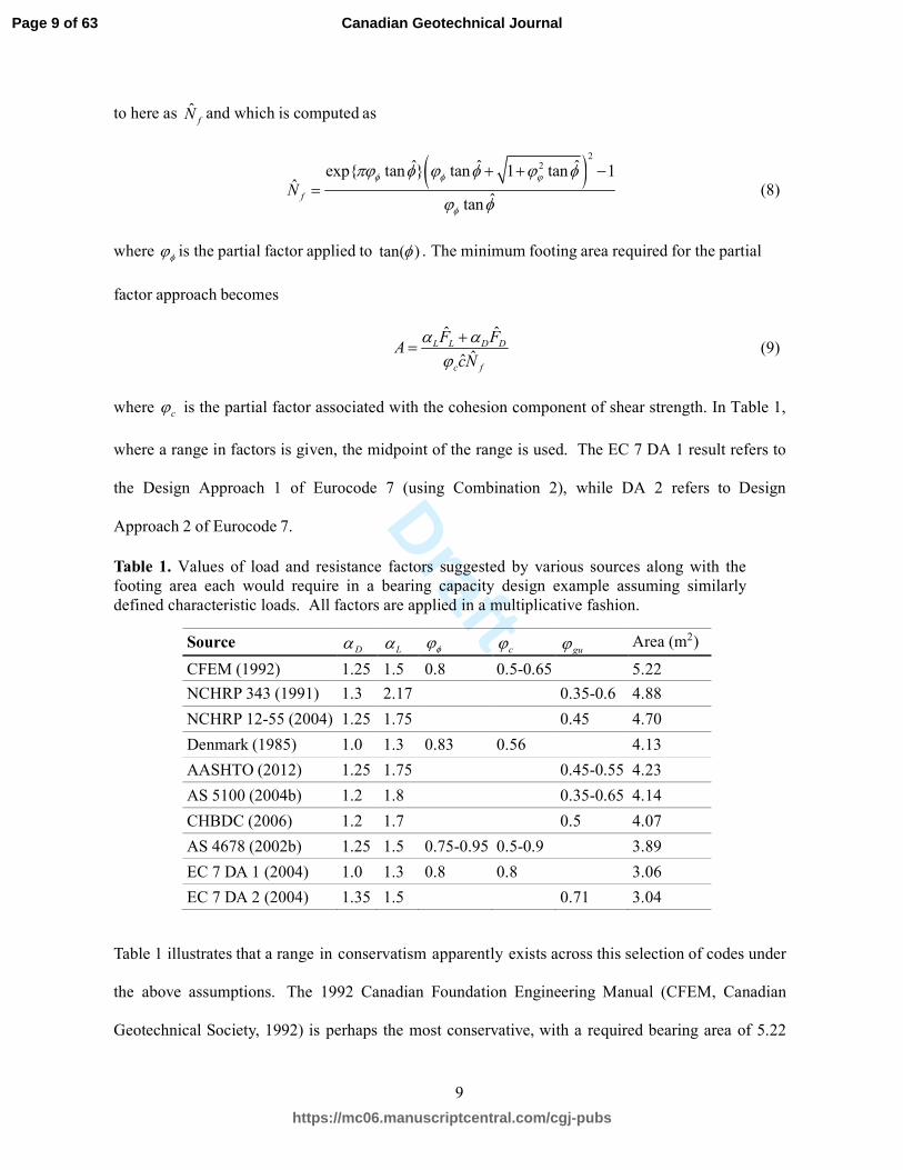
Table 1. Values of load and resistance factors suggested by various sources along with the
footing area each would require in a bearing capacity design example assuming similarly
defined characteristic loads. All factors are applied in a multiplicative fashion.
Source Dα Lα φϕ
cϕ guϕ Area (m2)
CFEM (1992) 1.25 1.5 0.8 0.5-0.65 5.22
NCHRP 343 (1991) 1.3 2.17 0.35-0.6 4.88
NCHRP 12-55 (2004) 1.25 1.75 0.45 4.70
Denmark (1985) 1.0 1.3 0.83 0.56 4.13
AASHTO (2012) 1.25 1.75 0.45-0.55 4.23
AS 5100 (2004b) 1.2 1.8 0.35-0.65 4.14
CHBDC (2006) 1.2 1.7 0.5 4.07
AS 4678 (2002b) 1.25 1.5 0.75-0.95 0.5-0.9 3.89
EC 7 DA 1 (2004) 1.0 1.3 0.8 0.8 3.06
EC 7 DA 2 (2004) 1.35 1.5 0.71 3.04
Table 1 illustrates that a range in conservatism apparently exists across this selection of codes under
the above assumptions. The 1992 Canadian Foundation Engineering Manual (CFEM, Canadian
Geotechnical Society, 1992) is perhaps the most conservative, with a required bearing area of 5.22
Page 9 of 63
https://mc06.manuscriptcentral.com/cgj-pubs
Canadian Geotechnical Journal
Draft
10
m2. The least conservative (apparently) are the two Design Approaches (DA 1 and 2) of Eurocode7
(2004) with required bearing areas of about 3.05 m2. However, Table 1 also assumes that the
characteristic design parameters are the same for all codes. A more complete comparison of the
levels of safety inherent in each design code involves a more careful consideration of how all of the
parameters entering the design process are defined and factored, particularly with respect to
characteristic values. Such a comparison is considered next.
2.1 Characteristic Loads and Bias Factors
Some codes specify that the characteristic load is equal to the mean, others suggest using a
‘cautious estimate of the mean’, while others specify the use of an upper (or lower) fractile
(whichever yields the most conservative result). Similarly, the characteristic resistance may be
computed using mean strength parameters, or using fractiles of the strength parameters. In general, the
difference between the characteristic design value and its mean is usually captured by a bias factor
defined as the ratio of the mean to characteristic value, i.e.,
, ,ˆ ˆ ˆ
R L DR L D
u L D
k k kR F F
µ µ µ= = = (10)
where k is the bias factor and µ is the mean of the subscripted variable. Introducing the dead to
live load ratio, / / D L D LR µ µ= , allows Eq. (3) to be re-expressed as
( )R s L DFµ µ µ≥ + (11)
where sF is now a global factor of safety, defined as
/
/
1
1
D D LR
L D D L
Ls
gu
Rk
k kF
R
ααϕ
= + +
(12)
Note that sF in Eq. (11) is seen to take on a similar role (and definition as ratio of mean
resistance to mean load) as does the traditional factor of safety used in working stress design
approaches. If the coefficients of variation of the loads and resistances are approximately the
Page 10 of 63
https://mc06.manuscriptcentral.com/cgj-pubs
Canadian Geotechnical Journal
Draft
11
same worldwide, then the global factor of safety provides a simple measure of the relative safety
of a code design which then allows the safety level of various codes to be compared. Ellingwood
(1999) notes that probability models for loads collected in research programs in North America
and Europe agree reasonably well, and so the assumption that coefficients of variation are
similar, at least between North America and Europe, is deemed to be reasonable. In this paper the
global factor of safety provided by the following design codes are compared for shallow foundations
at the bearing capacity ultimate limit state;
1) The National Building Code of Canada (NBCC) published by the National Research Council of
Canada (2010),
2) The Canadian Highway Bridge Design Code (CHBDC) published by the Canadian Standards
Association (2006),
3) AASHTO LRFD Bridge Design Specifications (AASHTO), published by the American
Association of State Highway and Transportation Officials (2012),
4) The Eurocodes, in particular EN 1990, which is Eurocode – Basis of Structural Design (CEN,
2002a) and provides the partial factors for the loads in all of the Eurocodes, including the partial
factors for loads in geotechnical designs, EN 1991-1-1, which is Eurocode 1: Actions on
Structures – Part 1-1: General Actions – Densities, self-weight, imposed loads for buildings
(CEN, 2002b) and Part 2: Traffic loads on bridges (CEN 2003), and EN 1997-1, which is
Eurocode 7 Geotechnical Design – Part 1: General Rules (CEN, 2004),
5) Australian Standard AS5100 Bridge Design (Standards Australia, 2004a
and 2004b)
To compare the level of safety between each of these codes, a hypothetical geotechnical system
having dead to live load ratio / 3.0D LR = is assumed.
Eurocode – Basis of structural design (EN 1990, CEN, 2002a) is reasonably specific as to how
characteristic loads are defined. With respect to dead loads, EN 1990 states that the variability of
Page 11 of 63
https://mc06.manuscriptcentral.com/cgj-pubs
Canadian Geotechnical Journal
Draft
12
permanent actions (i.e. dead loads) may be neglected if they do not vary significantly over the design
working life. In other words, if the coefficient of variation of dead loads,Dv , is less than about 10%,
then the dead loads can be considered to be non-random and ˆD DF µ= so that 1.0Dk = . The other
codes considered are less specific about the definition of characteristic dead loads, but generally
indicate that ˆDF is to be estimated using mean structural component weights. Bartlett et al. (2003)
suggest that often some dead load components are forgotten or missed in the estimation process, so
that in practice the characteristic (design) dead load is generally somewhat less than the true mean
dead load and the dead load bias factor is more like 1.05 (see also Ellingwood et al., 1980). For
highway bridges, Nowak (1994) suggests that the dead load bias factor ranges from 1.03 to 1.05,
which is in basic agreement with Bartlett’s estimate. Since a similar dead load estimation error is
probably common to all localities, it is assumed here that 1.05Dk = for all codes considered.
With respect to live loads, the North American codes define the characteristic live load as the
mean maximum live load exerted on the structure over its design lifetime – for example, Clause
4.3.1 of ASCE-7 (2010) states that uniformly distributed live loads are the mean of the maximum
load over the design lifetime. Although the NBCC does not specifically define the characteristic
live load, Bartlett et al. (2003) implies that it has the same definition as ASCE-7. Both codes
specify acceptable characteristic live load values which are typically somewhat higher than the
actual mean maximum live load. For example, both the Canadian and US codes specify a uniform
live load for office space of 2.4 kPa. Bartlett et al. (2003) suggest that, after reductions for influence
or tributary area, the code specified characteristic live load is typically about 10% higher than the
actual mean value, so that 0.9Lk = was adopted by Bartlett et al. in their calibration efforts for
the 2005 edition of the NBCC. As also reported by Bartlett et al., this bias value is in reasonable
agreement with ASCE-7. The AASHTO (2012) Bridge Design code takes its live load bias factor
from a detailed statistical analysis performed by Allen et al. (2005) who suggest that 0.95Lk = ,
Page 12 of 63
https://mc06.manuscriptcentral.com/cgj-pubs
Canadian Geotechnical Journal

Draft
13
which is reasonably close to the 0.9 given above for other North American codes. Similarly, Nowak
and Grouni (1994) show that the bias factor for live loads on Canadian bridges ranges from 0.85 to
1.0, depending on the span length, with an average of around 0.95Lk = .
EN 1990 (CEN, 2002a) states in Clause 4.1.2(7) that, for variable actions, the characteristic
value shall correspond to one of; an upper value with an intended probability of not being
exceeded or a lower value with an intended probability of being achieved, during some specific
reference period; or a nominal value, which may be specified in cases where a statistical
distribution is not known. This is a fairly vague definition, but Clause 4.1.2(4) suggests that an
“upper value” (which would be of interest for loads) corresponds to a 5% probability of being
exceeded (95% fractile). Clause 4.1.2(4) further states that the action may be assumed to be
Gaussian. If assumed Gaussian, then the 95% fractile is given by
ˆ 1 1.645 ( ) ( )1/ 1 1.645L L L L LF µ v k v= + = +→ (13)
where Lv is the coefficient of variation of the maximum lifetime live load. Both Allen (1975) and
Bartlett et al. (2003) use 0.27Lv = . The authors are not sure what value of Lv was assumed in the
Eurocode, but Ellingwood (1999) suggests that Europe uses a similar value to that used in North
America. If this is the case, then EN 1990 is using 0.69Lk = , which is very close to Allen’s (1975)
suggested bias of 0.7.
Another approach to estimating the live load bias factor employed in Europe, at least for
buildings, is to compare the characteristic office occupancy uniform live load specified in the
European and North American codes, which are 3.0 and 2.4 kPa, respectively. If the live load bias
factor of 0.9Lk = , adopted by Bartlett et al. (2003), is assumed true for North America, then
0.9 2.( )4 2.16Lµ = = kPa. If it is further assumed that this mean live load is at least approximately
true in Europe, then the European live load bias factor is 2.16 / 3.0 0.72Lk = = . On the basis of both
of the above approximate calculations, it appears likely, then, that EN 1990 uses a live load bias
Page 13 of 63
https://mc06.manuscriptcentral.com/cgj-pubs
Canadian Geotechnical Journal
Draft
14
factor of approximately 0.70Lk = . The authors were unable to determine the corresponding live
load bias factor for bridges in Europe, possibly because EN 1991-2 “Traffic loads on bridges”
(CEN, 2003) defines several load models which may individually have different bias factors. It is
assumed here that the Eurocodes maintain a relatively common bias factor of about 0.70Lk = across
all structure types.
The Australian Standard AS5100.1 (Standards Australia, 2004a) specifically defines load
actions for ultimate limit state as “an action having a 5% probability of exceedance in the design
life” in Clause 6.5. This is the same as used in the Eurocode (albeit more clearly specified). In
addition, since the Australian- New Zealand “Structural Design Actions” Standard AS/NZS 1170
(Standards Australia, 2002) specifies that the characteristic uniform live load for office buildings is
3.0 kPa, which is the same as the Eurocodes, it appears that the live load bias factor for Australia is
also 0.70Lk = .
2.2 Characteristic Resistance and Bias Factors
The estimation of the resistance of the ground to imposed loads is generally a multi-step process:
1) take measurements of the ground properties, 2) correlate the measurements with characteristic
engineering parameters (e.g. cohesion and friction angle), and 3) use the characteristic parameters in
a prediction model. Each step introduces errors, and so the characteristic resistance and associated
resistance factor (discussed later), along with the loads and load factors, must be determined in
such a way to ensure a safe design. Eurocode 7-1, Clause 2.4.5.2 (CEN, 2004) provides a number of
requirements for the selection of characteristic properties, such as “The characteristic value of a
geotechnical parameter shall be selected as a cautious estimate of the value affecting the occurrence of
the limit state” and “If statistical methods are used, the characteristic value should be derived such that
the calculated probability of a worse value governing the occurrence of the limit state under
consideration is not greater than 5%. NOTE: In this respect, a cautious estimate of the mean value is
Page 14 of 63
https://mc06.manuscriptcentral.com/cgj-pubs
Canadian Geotechnical Journal
Draft
15
a selection of the mean value of the limited set of geotechnical parameter values, with a confidence
level of 95%; where local failure is concerned, a cautious estimate of the low value is a 5% fractile.”
EN 1990 (CEN, 2002a) states that “where a low value of material or product property is
unfavorable, the characteristic value should be defined as the 5% fractile value.” According to
Schneider (2012), the characteristic values of ground parameters should be selected as a 5% fractile
value of the sample mean, using the distribution of the sample mean, rather than that of the samples
directly (the sample mean having standard deviation /s n , where s is the sample standard
deviation, and n is the number of samples used to estimate s). The authors note that a 5% fractile
value based on the sample mean will generally be quite a bit less conservative (i.e., closer to the
mean) than a 5% fractile based on the samples themselves.
Hicks (2013) interprets Clause 2.4.5.2 of Eurocode 7-1 as meaning that the characteristic
soil parameters are to be selected so as to ensure a 95% confidence in the geotechnical system
being designed, for any limit state. While this is a reasonable interpretation, it will involve both the
distribution of the applied maximum lifetime load and an appropriate spatial averaging of
geotechnical parameters over the actual failure surface (or failure domain). The authors feel that it is
probably easier at this point in time to develop a design code using characteristic soil parameters
based on fractiles of the soil parameter distribution.
In any case, the above discussion about characteristic values used in Eurocode 7 refers to the
selection of characteristic strength parameters (e.g. uc or φ ) rather than to the characteristic
resistance appearing in Eq. (3). The characteristic geotechnical resistance, ˆuR , would then be
computed employing a (probably non-linear) model which uses these characteristic ground
parameters. Thus, the final bias of the characteristic resistance depends not only on the distribution of
the ground properties, but also on the model used to predict ˆuR . It has been assumed here that the
coefficient of variation, vR , of ˆuR is approximately equal to the coefficient of variation of the ground
Page 15 of 63
https://mc06.manuscriptcentral.com/cgj-pubs
Canadian Geotechnical Journal

Draft
16
parameters used in the model, which are typically in the range of 0.1 to 0.3 (e.g., Meyerhof, 1995 and
Phoon and Kulhawy, 1999). Note that geotechnical resistance often involves an average of ground
properties, e.g. along a failure surface, which will have a smaller variability than the point
variability suggested in the literature. Thus, a reasonable value for the resistance variability is
deemed to be about 0.15Rv = , which is assumed here. Similar to Eq. (13), the resistance bias
factor assumed in the Eurocode can then be computed from
ˆ 1 1.645 1/ 1 1.64( ) ( 5 )u R R R RR µ v k v→= − = − (14)
which for 0.15Rv = gives 1.33Rk =
The Australian Standard AS5100.3 (Standards Australia, 2004b) states that “the characteristic
value of a geotechnical parameter should be a conservatively assessed value of the parameter.”
Although the authors were unable to find a more precise definition, the wording here suggests that
the Australians are following the Eurocode approach. Thus, a bias factor of 1.33Rk = has been
assumed for Australia as well.
In North America, Commentary Clause C10.4.6.1 of AASHTO (2012) says that “For strength
limit states, average measured values of relevant laboratory test data and/or in-situ test data were
used to calibrate the resistance factors”, which suggests that 1.0Rk = . However, the commentary
goes on to say that “it may not be possible to reliably estimate the average value of the properties
needed for design. In such cases, the Engineer may have no choice but to use a more conservative
selection of design properties” which suggests that in practice, 1.0Rk > .
Clause 8.5 of the Canadian Foundation Engineering Manual (Canadian Geotechnical Society,
2006) states that “Frequently, the mean value, or a value slightly less than the mean is selected by
geotechnical engineers as the characteristic value.” Commentary K of the NBCC User’s Guide
(National Research Council of Canada, 2011) says that “the [characteristic] resistance is the
engineer’s best estimate of the ultimate resistance.” Becker (1996a) claims “The design values do not
Page 16 of 63
https://mc06.manuscriptcentral.com/cgj-pubs
Canadian Geotechnical Journal
Draft
17
necessarily need to be taken as the mean values, although this is common geotechnical design
practice.” All of these statements suggest that 1.0Rk = , or perhaps slightly greater than 1.0. However,
Becker (1996a) later argues that the characteristic resistance is typically selected to be somewhat
below the mean, due to sampling uncertainties, and he subsequently uses kR = 1.1 in his NBCC
development paper (Becker, 1996b). Based on Becker’s reasoning, the value of 1.1Rk = is assumed
to apply to all of the North American design codes considered here.
2.3 Load Factors
Load factors are designed to reflect uncertainty in the lifetime loads experienced by a structure
or foundation. The basic idea is to set the factored loads, ˆL LFα and ˆ
D DFα , to values having
sufficiently low probability of being exceeded by the true (random) lifetime loads. Considering, for
example, live loads (with dead loads following the same reasoning), the factored live load that has
probability ε of being exceeded by the true live load over the design lifetime can be approximated
as
(ˆ 1 ) L L L LF µ z vεα = + (15)
in which zε is the standard normal point with exceedance probability ε , i.e., the point at which
( )zε εΦ − = , where Φ is the standard normal cumulative distribution function. Note that Eq. (15)
assumes that the live load is (at least approximately) normally distributed. Rearranging Eq. (15)
leads to an expression for the load factor, which is
(1 (1ˆ
) )LL LLL
L
µz v
Fk z vε εα
+
== +
(16)
ASCE-7 (American Society of Civil Engineers, 2010) found that their load factors are well
approximated by Eq. (16) when they set Lzε ω β= , where β is the target reliability index and
0.8Lω = when the live load is a principal action or 0.4Lω = when the live load is a companion
Page 17 of 63
https://mc06.manuscriptcentral.com/cgj-pubs
Canadian Geotechnical Journal

Draft
18
action. Equation (16) can be used for other load types simply by changing the subscript. Note that
Eq. (16) suggests that load factors are independent of the resistance distribution. It also states that the
load factors are very dependent on how the characteristic load is defined, i.e. on the load bias factor,
Lk . If designs have a common target reliability index, β , with 0.9Lk = in North America and
0.7Lk = in Europe and Australia, as suggested above, then one would expect the load factors in
Europe and Australia to be lower than those used in North America if Eq. (16) is accurate. As will
be seen, the European and Australian load factors are generally higher than those used in North
America – the European and Australian codes compensate for their higher load factors through
higher resistance factors. In other words, Eq. (16) cannot be used as a general formula for load
factors. The magnitude of the resistance factors (and bias factors) must still be considered.
Table 2 gives the load factors as specified by the various design codes considered here (using the
DA 2 partial factors for the Eurocode 7 GEO ultimate limit state). The last column of the table
gives the total load factor, Tα , for a given mean dead to live load ratio, which scales the total mean
load, L Dµ µ+ , to be equal to the sum of factored live and dead loads. The total load factor can be
seen in Eq. (12) and is defined by
/
/
1
1
D D L
L D L
L
D
T
R
k k Rα
αα = + +
(17)
Table 2. Load and bias factors for various design codes (assuming that / 3.0D LR = ).
Source Lk Dk Lα Dα Tα
NBCC 2010 0.9 1.05 1.50 1.25 1.31
CHBDC 2006 0.9 1.05 1.70 1.20 1.33
AASHTO 2012 0.95 1.05 1.75 1.25 1.35
Eurocode 7 DA 2 0.7 1.05 1.50 1.35 1.50
AS5100.3 0.7 1.05 1.80 1.20 1.50
The dead load factor for Eurocode 7, DA 2, (1.35) is larger than the dead load factors used in
Page 18 of 63
https://mc06.manuscriptcentral.com/cgj-pubs
Canadian Geotechnical Journal
Draft
19
North America (1.2 to 1.25) which, when combined with the smaller value of Lk , yields a
final Tα value that is significantly larger than that appearing in the Canadian codes and in
AASHTO. The Australian Standard AS5100 has an equivalently high Tα value because of its
relatively high live load factor, Tα , and low (assumed) live load bias factor,
Lk .
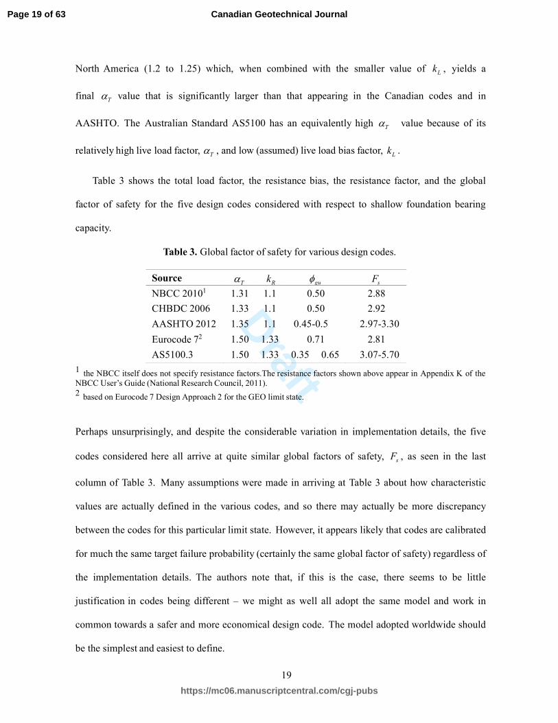
Table 3 shows the total load factor, the resistance bias, the resistance factor, and the global
factor of safety for the five design codes considered with respect to shallow foundation bearing
capacity.
Table 3. Global factor of safety for various design codes.
Source Tα Rk guφ sF
NBCC 20101 1.31 1.1 0.50 2.88
CHBDC 2006 1.33 1.1 0.50 2.92
AASHTO 2012 1.35 1.1 0.45-0.5 2.97-3.30
Eurocode 72 1.50 1.33 0.71 2.81
AS5100.3 1.50 1.33 0.35 0.65 3.07-5.70
1 the NBCC itself does not specify resistance factors.The resistance factors shown above appear in Appendix K of the
NBCC User’s Guide (National Research Council, 2011).
2 based on Eurocode 7 Design Approach 2 for the GEO limit state.
Perhaps unsurprisingly, and despite the considerable variation in implementation details, the five
codes considered here all arrive at quite similar global factors of safety, sF , as seen in the last
column of Table 3. Many assumptions were made in arriving at Table 3 about how characteristic
values are actually defined in the various codes, and so there may actually be more discrepancy
between the codes for this particular limit state. However, it appears likely that codes are calibrated
for much the same target failure probability (certainly the same global factor of safety) regardless of
the implementation details. The authors note that, if this is the case, there seems to be little
justification in codes being different – we might as well all adopt the same model and work in
common towards a safer and more economical design code. The model adopted worldwide should
be the simplest and easiest to define.
Page 19 of 63
https://mc06.manuscriptcentral.com/cgj-pubs
Canadian Geotechnical Journal
Draft
20
3. The 2014 Edition of the Canadian Highway Bridge Design Code
Geotechnical engineers are, of course, well aware of the fact that their designs depend on
one of the most uncertain of all engineering materials. Unlike wood, concrete, steel, and other
quality controlled engineering materials, it is not even known how the natural variability of soil
properties should properly be characterized. In addition, geotechnical engineers are also aware that
their uncertainty about the resistance of a geotechnical system decreases with increased site
understanding and site modeling effectiveness. Thus, there is a real desire amongst the geotechnical
community to have their designs reflect the degree of their site and modeling understanding. In other
words, geotechnical designs should become more economical as site and model understanding
increases. In this paper ‘site understanding’ refers to how well the ground providing the geotechnical
resistance is known and ‘model understanding’ means the degree of confidence that a designer has
in the (usually mathematical) model used to predict the geotechnical resistance.
To provide for designs that account for degree of understanding, it makes sense to have a
resistance factor which is adjusted as a function of site and model understanding. There are at least
two advantages to such an approach: 1) overall safety can be maintained at a common target
maximum failure probability, and 2) the direct economic advantage related to increasing site and
model understanding can be demonstrated. For example, the pre-2014 Canadian design codes
specify a single resistance factor for bearing capacity design (0.5). It doesn’t matter how confident
one is in one’s prediction of the bearing capacity of a foundation, the same resistance factor must be
used. Thus, there is no direct advantage to improving the geotechnical response prediction. If only a
single resistance factor can be used, one might as well spend the least amount of time one can on the
site investigation and modeling.
The resulting desire for a resistance factor which depends on site and model understanding is
not new. Littlejohn et al (1991) made the classic observation that “You pay for a site investigation
whether you have one or not,” which, as is well known, is very true. Recognizing this fact, it is of
Page 20 of 63
https://mc06.manuscriptcentral.com/cgj-pubs
Canadian Geotechnical Journal
Draft
21
real economic value to have a resistance factor which can be adjusted to reflect the true lifetime cost
of the lack or presence of an effective site investigation. The Australian Standard for Bridge Design,
Part 3: Foundations and Soil-Supporting Structures (AS5100.3, Standards Australia, 2004b) provide
a range of “geotechnical strength reduction factors” accompanied by guidance as to which end of
the scale should be used. For example, AS 5100.3 suggests that the lower end of the resistance
factor range (more conservative) should be used for limited site investigations, simple methods of
calculation, severe failure consequences, and so on. It is of interest to note that the Australian
Standard recommendations for the resistance factor considers both site and model understanding
along with failure consequence in their single factor. The idea of accommodating different levels of
site understanding also appears elsewhere in the literature. See, for example, the three-tier ground
variability classification provided by Phoon et al. (2003) and Phoon and Kulhawy (2008), where
residual ground variability can be thought of as reflecting the level of site understanding.
As is well known, the overall safety level of any design should depend on at least three things:
1) the uncertainty in the loads, 2) the uncertainty in the resistance, and 3) the severity of the failure
consequences. These three items are all usually deemed to be independent of one another and in
most modern codes are thus treated separately. Uncertainties in the loads are handled by load and load
combination factors, failure consequences are handled by applying a multiplicative importance factor
to the more site-specific and highly uncertain loads (e.g. earthquake, snow, and wind), and
uncertainties in resistance are handled by material specific resistance factors (e.g. cϕ for concrete, sϕ
for steel, etc).
Because the ground is also site-specific and highly uncertain, it makes sense to apply a partial
safety factor to the ground that depends on both the resistance uncertainty and consequence of
failure. This would be analogous to how wind load, for example, in the NBCC (NRC, 2010) has
both a load factor associated with wind speed uncertainty as well as an importance factor
associated with failure consequences. Figure 2 illustrates the basic idea, where the overall partial
Page 21 of 63
https://mc06.manuscriptcentral.com/cgj-pubs
Canadian Geotechnical Journal

Draft
22
factor applied to the geotechnical resistance varies with both site and model understanding and
failure consequence level. The numbers in the figure are relative to the default central partial factor
(i.e., relative to 1.0) and it is assumed that current geotechnical design approaches in Canada lead to
typical or default levels of site and model understanding so that, for typical failure consequence
geotechnical systems, the central value is what is currently used in design. From this value,
increased site investigation and/or modeling effort leads to higher understanding and a higher
overall partial factor (and so a more economical design). Similarly, for geotechnical systems
with high failure consequences, e.g. failure of the foundation of a major multi-lane highway bridge
in a large city, the overall partial factor is decreased to ensure a decreased maximum acceptable
failure probability. Of particular note in Figure 2 is the fact that if a geotechnical system with high
failure consequence is designed with low site and model understanding, the designer is penalized by a
low overall partial factor.
Figure 2. Floating partial safety factor, relative to the default, applied to geotechnical resistance
(numbers are for illustration only).
Figure 2 suggests that for each limit state (e.g. bearing, sliding, overturning, etc.) a 3 x 3 matrix
of resistance factors would have to be provided. Rather than introducing the resulting myriad tables,
the multiplicative approach taken in structural engineering (where the load is multiplied by both a
load factor and an importance factor) is adopted for geotechnical resistance as well in the 2014
Page 22 of 63
https://mc06.manuscriptcentral.com/cgj-pubs
Canadian Geotechnical Journal
Draft
23
CHBDC (CSA, 2014). In other words, the overall safety factor applied to geotechnical resistance is
broken into two parts;
1) a resistance factor, guϕ or
gsϕ , which accounts for resistance uncertainty. This factor basically
aims to achieve a target maximum acceptable failure probability equal to that used currently
for geotechnical designs for typical failure consequences (e.g., a lifetime failure probability of
1/5,000 or less). The subscript g refers to ‘geotechnical’ (or ‘ground’), while the subscripts u
and s refer to ultimate and serviceability limit states, respectively.
2) a consequence factor, Ψ , which accounts for failure consequences. Essentially, 1Ψ > if
failure consequences are low and 1Ψ < if failure consequences exceed those of typical
geotechnical systems. For typical systems, or where system importance is already accounted
for adequately by load importance factors, 1Ψ = . The basic idea of the consequence factor is
to adjust the maximum acceptable failure probability of the design down (e.g., to 1/10,000) for
high failure consequences, or up (e.g., to 1/1,000) for low failure consequences.
In the context of Figure 2, if the high consequence case were to be assigned a consequence factor
of 0.8, and the low understanding case assigned a resistance factor of 0.8, then the multiplication of
these two factors, 0.8 x 0.8 = 0.64, is approximately equal to the 0.6 value specified in the upper
left corner of Figure 2. In this way, the entire table can be expressed by two independent factors,
each having three values.
The geotechnical design would then proceed by ensuring that the factored geotechnical
resistance at least equals the effect of factored loads. For example, for ultimate limit states, this
means that in the 2014 CHBDC the geotechnical design will need to satisfy an equation of the form
ˆ ˆgu i i ui ui
i
R I Fϕ ηαΨ ≥∑ (18)
which is almost identical to Eq. (2), with the exception that the overall geotechnical resistance
factor is expressed as the product of the consequence factor, Ψ , and the ultimate geotechnical
Page 23 of 63
https://mc06.manuscriptcentral.com/cgj-pubs
Canadian Geotechnical Journal
Draft
24
resistance factor, guϕ , and the loads and load factors appearing on the right-hand-side are also those
specific for the ultimate limit state under consideration (and, hence, the subscript u). An entirely
similar equation must be satisfied for serviceability limit states, with the subscript u replaced by s.
The serviceability geotechnical resistance factors, gsϕ , will be closer to 1.0 than
guϕ , since
serviceability limit states can have larger maximum acceptable probabilities of occurrence.
Note that Eq. (18) simultaneously specifies a consequence factor, Ψ , and an importance
factor, iI , both of which aim to modify failure probability as a function of failure consequence. As
mentioned previously, the basic idea of the importance factor in North America is to account for
the high variability of site-specific wind, snow, and seismic loads for differing failure
consequences. Since the ground is also a highly variable site-specific parameter, it similarly needs
to be specifically factored to account for failure consequences. How the two factors, and iIΨ ,
should interact is still under research. The 2014 CHBDC states that if 1iI > , then Ψ should be set
to 1.0.
The geotechnical resistance factor, guϕ or
gsϕ , depends on the degree of site and prediction
model understanding. Three levels are considered in the 2014 CHBDC;
• High understanding: extensive project-specific investigation procedures and/or
knowledge are combined with prediction models of demonstrated quality to achieve a
high level of confidence with performance predictions,
• Typical understanding: typical project-specific investigation procedures and/or
knowledge are combined with conventional prediction models to achieve a typical level
of confidence with performance predictions,
• Low understanding: limited representative information (e.g. previous experience,
extrapolation from nearby and/or similar sites, etc.) combined with conventional
prediction models to achieve a lower level of confidence with performance predictions.
Page 24 of 63
https://mc06.manuscriptcentral.com/cgj-pubs
Canadian Geotechnical Journal
Draft
25
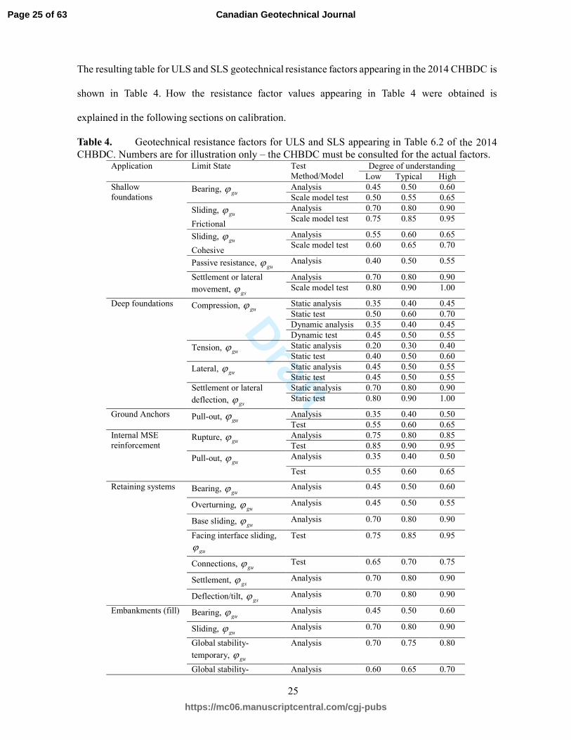
The resulting table for ULS and SLS geotechnical resistance factors appearing in the 2014 CHBDC is
shown in Table 4. How the resistance factor values appearing in Table 4 were obtained is
explained in the following sections on calibration.
Table 4. Geotechnical resistance factors for ULS and SLS appearing in Table 6.2 of the 2014
CHBDC. Numbers are for illustration only – the CHBDC must be consulted for the actual factors. Application Limit State Test
Method/Model
Degree of understanding
Low Typical High
Shallow
foundations Bearing,
guϕ Analysis 0.45 0.50 0.60
Scale model test 0.50 0.55 0.65
Sliding, guϕ
Frictional
Analysis 0.70 0.80 0.90
Scale model test 0.75 0.85 0.95
Sliding, guϕ
Cohesive
Analysis 0.55 0.60 0.65
Scale model test 0.60 0.65 0.70
Passive resistance, guϕ Analysis 0.40 0.50 0.55
Settlement or lateral
movement, gsϕ
Analysis 0.70 0.80 0.90
Scale model test 0.80 0.90 1.00
Deep foundations Compression, guϕ Static analysis 0.35 0.40 0.45
Static test 0.50 0.60 0.70
Dynamic analysis 0.35 0.40 0.45
Dynamic test 0.45 0.50 0.55
Tension, guϕ Static analysis 0.20 0.30 0.40
Static test 0.40 0.50 0.60
Lateral, guϕ Static analysis 0.45 0.50 0.55
Static test 0.45 0.50 0.55
Settlement or lateral
deflection, gsϕ
Static analysis 0.70 0.80 0.90
Static test 0.80 0.90 1.00
Ground Anchors Pull-out, guϕ Analysis 0.35 0.40 0.50
Test 0.55 0.60 0.65
Internal MSE
reinforcement Rupture,
guϕ Analysis 0.75 0.80 0.85
Test 0.85 0.90 0.95
Pull-out, guϕ Analysis 0.35 0.40 0.50
Test 0.55 0.60 0.65
Retaining systems Bearing, guϕ Analysis 0.45 0.50 0.60
Overturning, guϕ Analysis 0.45 0.50 0.55
Base sliding, guϕ Analysis 0.70 0.80 0.90
Facing interface sliding,
guϕ
Test 0.75 0.85 0.95
Connections, guϕ Test 0.65 0.70 0.75
Settlement, gsϕ Analysis 0.70 0.80 0.90
Deflection/tilt, gsϕ Analysis 0.70 0.80 0.90
Embankments (fill) Bearing, guϕ Analysis 0.45 0.50 0.60
Sliding, guϕ Analysis 0.70 0.80 0.90
Global stability-
temporary, guϕ
Analysis 0.70 0.75 0.80
Global stability- Analysis 0.60 0.65 0.70
Page 25 of 63
https://mc06.manuscriptcentral.com/cgj-pubs
Canadian Geotechnical Journal

Draft
26
permanent, guϕ
Settlement, gsϕ Analysis 0.70 0.80 0.90
Test 0.80 0.90 1.00
The consequence factor, Ψ , appearing in Eq. (18), adjusts the maximum acceptable failure
probability of the geotechnical system being designed to a value which is appropriate for the
magnitude of the failure consequences. Three failure consequence levels are considered in the 2014
CHBDC;
• High consequence: the foundations and/or geotechnical systems are designed for applications,
including bridges, essential to post-disaster recovery (e.g. lifeline) and/or having large
societal or economic impacts.
• Typical consequence: the foundations and/or geotechnical systems are designed for
applications, including bridges, carrying medium to large volumes of traffic and/or having
potential impacts on alternative transportation corridors or structures.
• Low consequence: the foundations and/or geotechnical systems are designed for
applications carrying low volumes of traffic and having limited impacts on alternative
transportation corridors.
These failure consequence definitions are somewhat in agreement with the “importance
definitions” appearing in the seismic design (Section 4) provisions of the 2014 CHBDC, which
specify the following;
• Major-route bridge: Structure that is on a route that is critical to facilitate post-disaster
emergency response, security and defence purposes, and subsequent economic recovery. The
route is a key component of the regional transportation network.
• Lifeline bridge: Unique and/or very large structure that represents a major investment and
would be time-consuming to repair or replace. Note: A lifeline bridge is vital to the integrity
of the regional transportation network, the ongoing economy and security of the region.
• Other bridge: a structure that does not fall into the importance categories of Lifeline or
Page 26 of 63
https://mc06.manuscriptcentral.com/cgj-pubs
Canadian Geotechnical Journal
Draft
27
Major-route bridges
The seismic design (Section 4) definitions for “Major-route”, “Lifeline” and “Other” are
similar to the definitions for “High”, “Typical”, and “Low”, given for geotechnical design (Section
6), respectively. However, there is little way to compare the definitions in the two sections, since no
performance reliability targets were available for the three importance levels in Section 4 at the time
of writing. Efforts are ongoing to bring the sections into harmony.
In Eq. (18), the value of Ψ is not subscripted by u nor by s, which implies that it is independent of
the ultimate and serviceability limit states. Preliminary evidence that Ψ is independent of the
limit state is at least true for deep foundations has been provided by Naghibi et al. (2013). Although
it is not known if this independence also holds for other geotechnical systems and limit states, it
does seem to be reasonable that it would. For example, a typical geotechnical system might have a
target maximum lifetime failure probability of 1/5, 000 for an ultimate limit state, but only
1/500 for a serviceability limit state. If the geotechnical system has high failure consequences, the
lifetime maximum acceptable failure probability might decrease by the same fraction for both limit
states; i.e. to 1/10, 000 for ULS and to 1/1, 000 for SLS. Thus, it seems reasonable that the same
(or quite similar) consequence factor can be used to adjust the target maximum acceptable failure
probabilities for both ULS and SLS designs, since the probabilities scale by the same fraction.
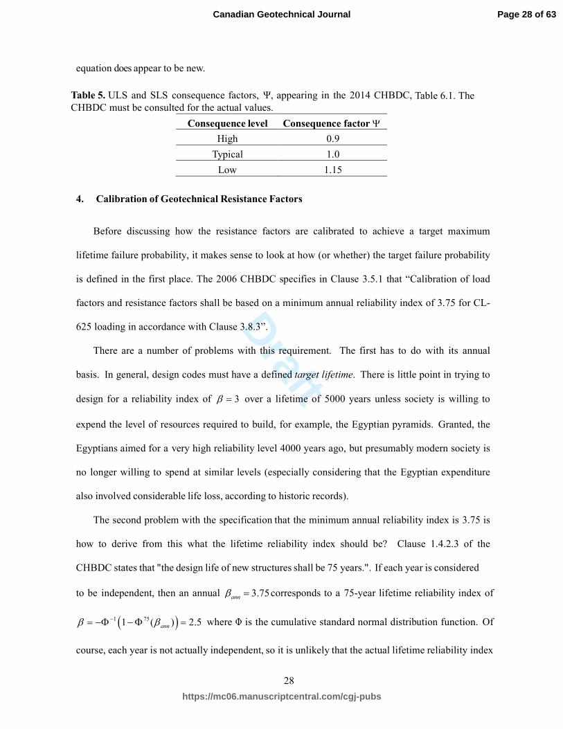
The consequence factors specified in the 2014 CHBDC for the three consequence levels are
shown in Table 5. How the values are determined will be discussed shortly. This table is very
similar to Table B3 in EN 1990 (CEN, 2002a) which specifies three multiplicative factors, 0.9,
1.0, and 1.1, to be applied to loads (actions) for low, medium, and high failure consequences,
respectively (these factors are approximately the inverse of the factors seen in Table 5 because they
appear on the load side of the LRFD equation). In other words, the concept of shifting the target
failure probability to account for severity of failure consequences is certainly not new, although the
application of the consequence factor to the resistance side, rather than the load side, of the LRFD
Page 27 of 63
https://mc06.manuscriptcentral.com/cgj-pubs
Canadian Geotechnical Journal
Draft
28
equation does appear to be new.
Table 5. ULS and SLS consequence factors, Ψ, appearing in the 2014 CHBDC, Table 6.1. The
CHBDC must be consulted for the actual values.
Consequence level Consequence factor Ψ
High 0.9
Typical 1.0
Low 1.15
4. Calibration of Geotechnical Resistance Factors
Before discussing how the resistance factors are calibrated to achieve a target maximum
lifetime failure probability, it makes sense to look at how (or whether) the target failure probability
is defined in the first place. The 2006 CHBDC specifies in Clause 3.5.1 that “Calibration of load
factors and resistance factors shall be based on a minimum annual reliability index of 3.75 for CL-
625 loading in accordance with Clause 3.8.3”.
There are a number of problems with this requirement. The first has to do with its annual
basis. In general, design codes must have a defined target lifetime. There is little point in trying to
design for a reliability index of 3β = over a lifetime of 5000 years unless society is willing to
expend the level of resources required to build, for example, the Egyptian pyramids. Granted, the
Egyptians aimed for a very high reliability level 4000 years ago, but presumably modern society is
no longer willing to spend at similar levels (especially considering that the Egyptian expenditure
also involved considerable life loss, according to historic records).
The second problem with the specification that the minimum annual reliability index is 3.75 is
how to derive from this what the lifetime reliability index should be? Clause 1.4.2.3 of the
CHBDC states that "the design life of new structures shall be 75 years.". If each year is considered
to be independent, then an annual 3.75annβ = corresponds to a 75-year lifetime reliability index of
( )1 751 ( ) 2.5annβ β−= −Φ −Φ = where Φ is the cumulative standard normal distribution function. Of
course, each year is not actually independent, so it is unlikely that the actual lifetime reliability index
Page 28 of 63
https://mc06.manuscriptcentral.com/cgj-pubs
Canadian Geotechnical Journal

Draft
29
suggested by Clause 3.5.1 is as low as 2.5. To determine the actual lifetime reliability index, one has
to consider the time variability of both the loads and the resistance. Table B2 in EN 1990 (CEN,
2002a) provides target reliability indices for high, medium, and low failure consequences both
annually and for a 50-year lifetime. Of interest is the fact that the 50-year lifetime target
reliability indices in EN 1990 are computed from the annual reliability indices assuming
independence between years.
It has been argued that the resistances of the structure and geotechnical systems remain
relatively constant with time. However, anybody who has looked at an older bridge in Canada
knows that this is evidently not true. Both the structural and geotechnical systems often exhibit
substantial degradation over a 75 year period. Certainly, geotechnical systems are continually
degraded by pore-pressure variations, freeze-thaw effects, erosion, seismic motion, local
liquefaction, and so on. Thus, even if the annual reliability index of 3.75 is achieved in the first
year after construction, the 75-year reliability index will certainly be lower. The actual 75-year
reliability index will be somewhere between 2.5, assuming independence (as assumed in EN 1990),
and 3.75, which assumes neither degradation nor fluctuation in loads. Although what the actual
lifetime reliability should be needs further research, it seems reasonable to assume a lifetime
reliability index between 3.0 and 3.5 would conservatively correspond to an annual reliability
index of 3.75. The theoretical calibration exercises described in this and the following section will
target a 75-year lifetime reliability index of a typical structure to be approximately 3.5, at least
theoretically.
The calibration of the resistance factors appearing in the 2014 edition of the CHBDC includes
the following considerations;
1) It is, of course, clear that probabilistic theories are only as good as their assumptions
and that most of the assumptions in geotechnical engineering are fraught with
uncertainties. For example, the SLS design of a foundation frequently does not involve
Page 29 of 63
https://mc06.manuscriptcentral.com/cgj-pubs
Canadian Geotechnical Journal
Draft
30
estimating the foundation settlement at all. Rather, the maximum SLS load on the
foundation is often assumed to be 1/3 of the maximum ULS load, which typically results in
a very conservative SLS design (see, e.g., pg 254 of French, 1999). Such conservatism
should not then be compounded by applying an SLS resistance factor obtained using a best
estimate of the actual (non-conservative) foundation settlement.
2) The primary value of probabilistic methods is that they provide a rational approach to
com-paring designs, in terms of relative safety. Thus, any code factor calibration should
start with existing code values, since they have been shown over time to be reasonable
and societally acceptable, and then adjust the existing values to rationally account for
uncertainty and failure consequences.
The resistance factor calibration must therefore start with a review of the factors currently
used in Canadian geotechnical design codes, as well as those used in other codes from around the
world, along the lines of the comparison presented in the “Comparison to Other Codes” Section.
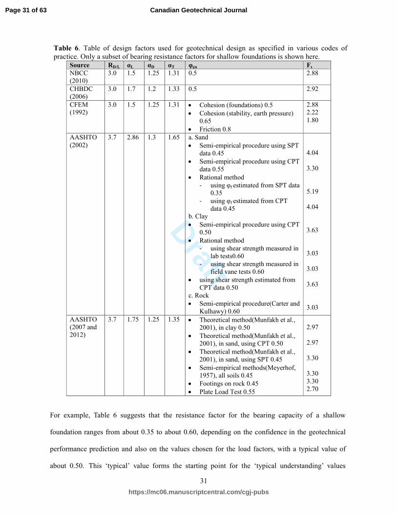
Table 6 illustrates such a review, where the rightmost column provides the total resistance factor
estimated for each code using Eq. (12). Table 3 is a subset of Table 6 and Table 6 is a small subset
of a much more extensive table that was prepared to compare the load and geotechnical resistance
factors between a variety of codes, reports, and manuals from various jurisdictions. The complete
table can be found at [URL to be provided by CGJ].
In the calibration process, Table 6, and its more extensive counterpart at the URL given above, is
used to suggest the ‘best’ currently acceptable estimates of ‘typical’ resistance factors. These are the
factors that have been found to lead to societally acceptable failure probabilities under current
design practice.
Page 30 of 63
https://mc06.manuscriptcentral.com/cgj-pubs
Canadian Geotechnical Journal
Draft
31
Table 6. Table of design factors used for geotechnical design as specified in various codes of
practice. Only a subset of bearing resistance factors for shallow foundations is shown here.
Source RD/L αL αD αT φgu Fs
NBCC
(2010)
3.0 1.5 1.25 1.31 0.5 2.88
CHBDC (2006)
3.0 1.7 1.2 1.33 0.5 2.92
CFEM (1992)
3.0 1.5 1.25 1.31 • Cohesion (foundations) 0.5
• Cohesion (stability, earth pressure)
0.65
• Friction 0.8
2.88 2.22
1.80
AASHTO
(2002)
3.7 2.86 1.3 1.65 a. Sand
• Semi-empirical procedure using SPT
data 0.45
• Semi-empirical procedure using CPT
data 0.55
• Rational method
- using φf estimated from SPT data
0.35
- using φf estimated from CPT
data 0.45 b. Clay
• Semi-empirical procedure using CPT
0.50
• Rational method
- using shear strength measured in
lab tests0.60
- using shear strength measured in
field vane tests 0.60
• using shear strength estimated from
CPT data 0.50
c. Rock
• Semi-empirical procedure(Carter and
Kulhawy) 0.60
4.04
3.30
5.19
4.04
3.63
3.03
3.03
3.63
3.03
AASHTO
(2007 and 2012)
3.7 1.75 1.25 1.35 • Theoretical method(Munfakh et al.,
2001), in clay 0.50
• Theoretical method(Munfakh et al.,
2001), in sand, using CPT 0.50
• Theoretical method(Munfakh et al.,
2001), in sand, using SPT 0.45
• Semi-empirical methods(Meyerhof,
1957), all soils 0.45
• Footings on rock 0.45
• Plate Load Test 0.55
2.97
2.97
3.30
3.30
3.30
2.70
For example, Table 6 suggests that the resistance factor for the bearing capacity of a shallow
foundation ranges from about 0.35 to about 0.60, depending on the confidence in the geotechnical
performance prediction and also on the values chosen for the load factors, with a typical value of
about 0.50. This ‘typical’ value forms the starting point for the ‘typical understanding’ values
Page 31 of 63
https://mc06.manuscriptcentral.com/cgj-pubs
Canadian Geotechnical Journal

Draft
32
appearing in Table 4. The range suggested in Table 6 provides some insight into the range that might
be appropriate for the three levels of site and model understanding considered in the 2014 CHBDC.
Once the typical resistance factor values have been established, the next two steps are to look at
how the resistance factors should change as a result of changes in the level of site and model
understanding, and how the consequence factor should be set to reflect changes in the failure
consequence severity. This paper will not attempt to report on all of the research relating to these
two steps, but will rather concentrate on the results relating to one particular limit state, namely the
bearing capacity of a shallow foundation, which has been a common example used throughout this
paper to illustrate the calibration process.
The question of how the resistance factor should be adjusted as the level of site and model
understanding changes brings up the question of how the reliability of a geotechnical design can be
estimated in the first place, for any given level of site and model understanding. While statistical
estimates of reliability rely on multiple realizations of the random outcome (in this case, failure
or non-failure of the particular design in question), we usually have only one ‘realization’, which is
the as-designed and constructed geotechnical system. If that system fails, it is difficult to say if
failure was due to a poor design model or just due to exceptional ‘random’ events. To assess the
reliability of a geotechnical design, the use of properly designed Monte Carlo simulations is an
essential tool, since it allows the direct estimation of the design performance distribution due to
changes in the level of site and model understanding.
The approach used here is essentially to use Monte Carlo simulations, modeling the ground as
a spatially varying random field, and carry out a virtual site investigation, design, and construction
of the geotechnical system. The geotechnical system is then subjected to random maximum
lifetime loads and checked to see if the particular limit state under investigation is exceeded. If so,
a failure is recorded and the process is repeated. The failure probability of the design is then
estimated as the number of failures divided by the number of trials – if the failure probability is
Page 32 of 63
https://mc06.manuscriptcentral.com/cgj-pubs
Canadian Geotechnical Journal

Draft
33
too high, the design factors are suitably adjusted, and so on. The detailed steps are as follows;
1) for a particular geotechnical system (e.g., shallow foundation) and limit state (e.g., bearing
capacity), choose a resistance factor to be used in the design,
2) simulate a random field of ground properties, having a specified variance and correlation
structure,
3) virtually sample the ground at some location to obtain ‘observations’ of the ground properties.
The distance between the sample and the geotechnical system acts as a proxy for site and
model understanding – the farther the sample is from the geotechnical system, the more the
uncertainty about the system performance (decreased site and model understanding),
4) design the geotechnical system using the characteristic geotechnical parameters determined
from the sample taken in step 3. The definition of ‘characteristic’ depends on the design
code being used. For example, in Europe, the characteristic values might be a lower 5-
percentile for local failures, or more generally a cautious estimate of the value affecting the
occurrence of the limit state. In North America, a ‘cautious estimate of the mean’ is
probably a more common definition, as discussed previously. In most of the calibration
exercises undertaken for the CHBDC, the characteristic values were taken as the geometric
average of the sampled ‘observations’. The geometric average is always at least slightly
lower (more so for higher variability) than the arithmetic average, and so can be viewed as a
‘cautious estimate of the mean’,
5) virtually construct the geotechnical system according to the design in the previous step and
place it on (or in) the random field generated in step 2,
6) employ a sophisticated numerical model (e.g., the finite element method) to determine if the
geotechnical system exceeds the limit state being designed against (this is a failure),
7) repeat from step 2 a large number of times, recording the number of failures.
8) the probability of failure is then estimated as the number of failures divided by the number of
Page 33 of 63
https://mc06.manuscriptcentral.com/cgj-pubs
Canadian Geotechnical Journal
Draft
34
trials. If this probability is too high, the resistance factor needs to be decreased, if too low,
the resistance factor can be increased. After adjusting the resistance factor appropriately, the
entire procedure can be repeated from step 1 using the new resistance factor.
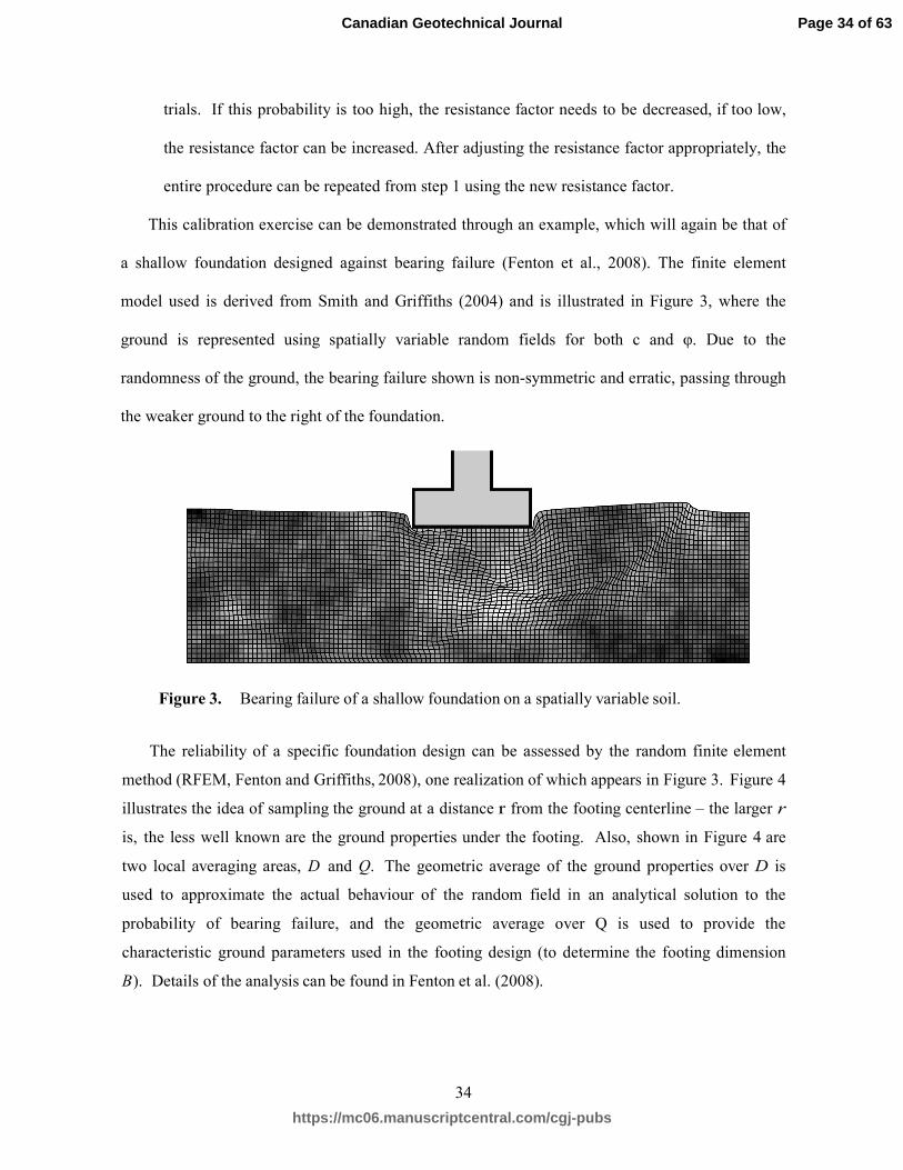
This calibration exercise can be demonstrated through an example, which will again be that of
a shallow foundation designed against bearing failure (Fenton et al., 2008). The finite element
model used is derived from Smith and Griffiths (2004) and is illustrated in Figure 3, where the
ground is represented using spatially variable random fields for both c and φ. Due to the
randomness of the ground, the bearing failure shown is non-symmetric and erratic, passing through
the weaker ground to the right of the foundation.
Figure 3. Bearing failure of a shallow foundation on a spatially variable soil.
The reliability of a specific foundation design can be assessed by the random finite element
method (RFEM, Fenton and Griffiths, 2008), one realization of which appears in Figure 3. Figure 4
illustrates the idea of sampling the ground at a distance r from the footing centerline – the larger r
is, the less well known are the ground properties under the footing. Also, shown in Figure 4 are
two local averaging areas, D and Q. The geometric average of the ground properties over D is
used to approximate the actual behaviour of the random field in an analytical solution to the
probability of bearing failure, and the geometric average over Q is used to provide the
characteristic ground parameters used in the footing design (to determine the footing dimension
B). Details of the analysis can be found in Fenton et al. (2008).
Page 34 of 63
https://mc06.manuscriptcentral.com/cgj-pubs
Canadian Geotechnical Journal

Draft
35
Figure 4. Locations of footing and sample used in the calibration of bearing capacity resistance
factors.
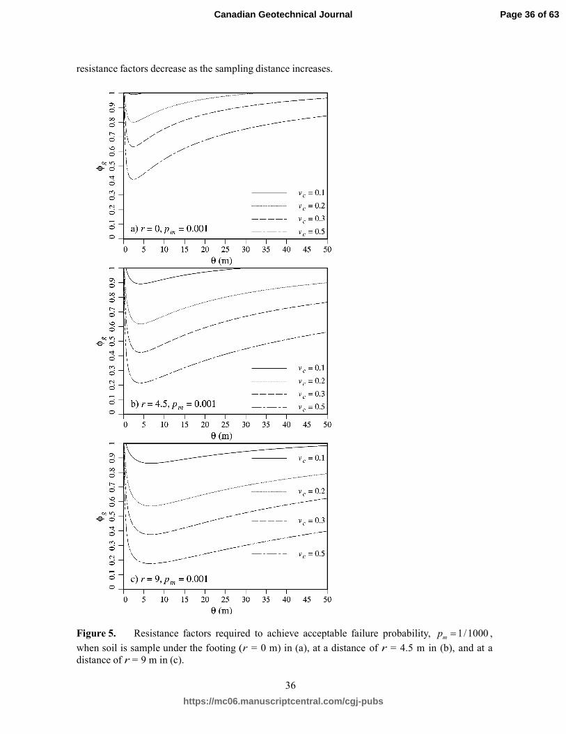
Figure 5 presents the theoretically determined resistance factors for the case where the target
maximum lifetime failure probability is 0.001mp = , which corresponds to a reliability index of
about 3.1β = . Note that this is somewhat below the target lifetime reliability index of 3.5 (the
study did not include 3.5β = ) so that the resistance factors will be slightly higher than those
theoretically appropriate for 3.5β = . However, as mentioned previously, interest is primarily in
how the resistance factor changes as the level of site understanding changes, and not on the actual
magnitude of the theoretical resistance factors, since these are unlikely to be exactly the same as the
currently accepted resistance factors in any case.
The three plots in Figure 5 correspond to the ground being sampled directly under the footing
(r = 0) in (a), the sample taken at a moderate distance from the footing (r = 4.5 m) in (b), and
the sample taken at a larger distance from the footing (r = 9 m) in (c). As expected, the required
Page 35 of 63
https://mc06.manuscriptcentral.com/cgj-pubs
Canadian Geotechnical Journal
Draft
36
resistance factors decrease as the sampling distance increases.
Figure 5. Resistance factors required to achieve acceptable failure probability, 1/1000mp = ,
when soil is sample under the footing (r = 0 m) in (a), at a distance of r = 4.5 m in (b), and at a
distance of r = 9 m in (c).
Page 36 of 63
https://mc06.manuscriptcentral.com/cgj-pubs
Canadian Geotechnical Journal
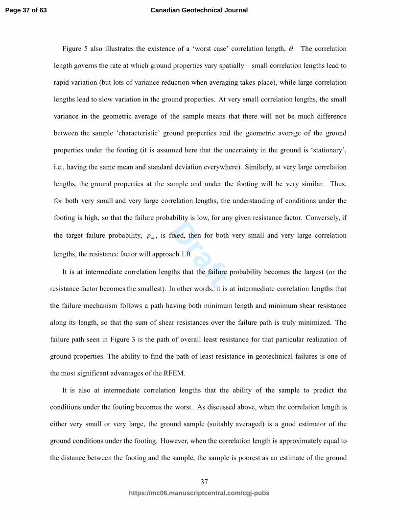
Draft
37
Figure 5 also illustrates the existence of a ‘worst case’ correlation length, θ . The correlation
length governs the rate at which ground properties vary spatially – small correlation lengths lead to
rapid variation (but lots of variance reduction when averaging takes place), while large correlation
lengths lead to slow variation in the ground properties. At very small correlation lengths, the small
variance in the geometric average of the sample means that there will not be much difference
between the sample ‘characteristic’ ground properties and the geometric average of the ground
properties under the footing (it is assumed here that the uncertainty in the ground is ‘stationary’,
i.e., having the same mean and standard deviation everywhere). Similarly, at very large correlation
lengths, the ground properties at the sample and under the footing will be very similar. Thus,
for both very small and very large correlation lengths, the understanding of conditions under the
footing is high, so that the failure probability is low, for any given resistance factor. Conversely, if
the target failure probability, mp , is fixed, then for both very small and very large correlation
lengths, the resistance factor will approach 1.0.
It is at intermediate correlation lengths that the failure probability becomes the largest (or the
resistance factor becomes the smallest). In other words, it is at intermediate correlation lengths that
the failure mechanism follows a path having both minimum length and minimum shear resistance
along its length, so that the sum of shear resistances over the failure path is truly minimized. The
failure path seen in Figure 3 is the path of overall least resistance for that particular realization of
ground properties. The ability to find the path of least resistance in geotechnical failures is one of
the most significant advantages of the RFEM.
It is also at intermediate correlation lengths that the ability of the sample to predict the
conditions under the footing becomes the worst. As discussed above, when the correlation length is
either very small or very large, the ground sample (suitably averaged) is a good estimator of the
ground conditions under the footing. However, when the correlation length is approximately equal to
the distance between the footing and the sample, the sample is poorest as an estimate of the ground
Page 37 of 63
https://mc06.manuscriptcentral.com/cgj-pubs
Canadian Geotechnical Journal
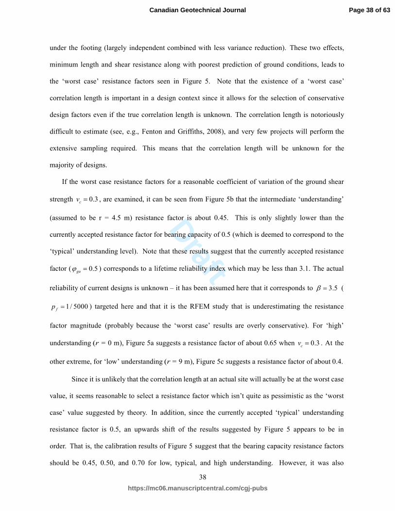
Draft
38
under the footing (largely independent combined with less variance reduction). These two effects,
minimum length and shear resistance along with poorest prediction of ground conditions, leads to
the ‘worst case’ resistance factors seen in Figure 5. Note that the existence of a ‘worst case’
correlation length is important in a design context since it allows for the selection of conservative
design factors even if the true correlation length is unknown. The correlation length is notoriously
difficult to estimate (see, e.g., Fenton and Griffiths, 2008), and very few projects will perform the
extensive sampling required. This means that the correlation length will be unknown for the
majority of designs.
If the worst case resistance factors for a reasonable coefficient of variation of the ground shear
strength 0.3cv = , are examined, it can be seen from Figure 5b that the intermediate ‘understanding’
(assumed to be r = 4.5 m) resistance factor is about 0.45. This is only slightly lower than the
currently accepted resistance factor for bearing capacity of 0.5 (which is deemed to correspond to the
‘typical’ understanding level). Note that these results suggest that the currently accepted resistance
factor ( 0.5guϕ = ) corresponds to a lifetime reliability index which may be less than 3.1. The actual
reliability of current designs is unknown – it has been assumed here that it corresponds to 3.5β = (
1/ 5000fp = ) targeted here and that it is the RFEM study that is underestimating the resistance
factor magnitude (probably because the ‘worst case’ results are overly conservative). For ‘high’
understanding (r = 0 m), Figure 5a suggests a resistance factor of about 0.65 when 0.3cv = . At the
other extreme, for ‘low’ understanding (r = 9 m), Figure 5c suggests a resistance factor of about 0.4.
Since it is unlikely that the correlation length at an actual site will actually be at the worst case
value, it seems reasonable to select a resistance factor which isn’t quite as pessimistic as the ‘worst
case’ value suggested by theory. In addition, since the currently accepted ‘typical’ understanding
resistance factor is 0.5, an upwards shift of the results suggested by Figure 5 appears to be in
order. That is, the calibration results of Figure 5 suggest that the bearing capacity resistance factors
should be 0.45, 0.50, and 0.70 for low, typical, and high understanding. However, it was also
Page 38 of 63
https://mc06.manuscriptcentral.com/cgj-pubs
Canadian Geotechnical Journal
Draft
39
felt that perhaps using a resistance factor as high as 0.70 for the ‘high’ understanding case was
overly optimistic, especially considering the fact that measurement errors begin to be important
when r = 0 m, and measurement errors were ignored in this RFEM study. As a result, the ‘high’
understanding resistance factor was lowered to be 0.60 in the 2014 CHBDC. This adjustment was felt
to be reasonably conservative.
A similar calibration exercise was carried out for the limit states where associated RFEM
studies were available. These are;
1) resistance factors for the ULS design of deep foundations (Fenton and Naghibi 2011;
Naghibi and Fenton 2011),
2) resistance factors for the settlement design of shallow foundations (Fenton et al.
2005a),
3) resistance factors for the settlement design of deep foundations (Naghibi et al. 2014),
4) effect of site sampling on the failure probability of retaining walls (Fenton et al.
2005b).
The high and low understanding resistance factors for limit states not having an associated RFEM
study were obtained through judgment and experience with similar limit state results.
5. Calibration of the Geotechnical Consequence Factor
The basic idea of the consequence factor is to adjust the target maximum lifetime failure
probability, pm, to a value which is appropriate for the failure consequences. For example, if the
geotechnical system supports a storage warehouse which is rarely visited, the failure consequences
are slight and its failure probability should be higher than that for typically supported structures.
If, on the other hand, the geotechnical system supports a hospital or lifeline bridge, then the failure
probability should probably be lower than that for typically supported structures. The maximum
lifetime failure probabilities targeted in the 2014 CHBDC for geotechnical design are as shown in
Page 39 of 63
https://mc06.manuscriptcentral.com/cgj-pubs
Canadian Geotechnical Journal
Draft
40
Table 7. The target reliability indices reported in EN 1990 (CEN, 2002a) are 4.3, 3.8, and 3.3 for
ULS designs at high, typical, and low consequence levels. These targets are somewhat higher than
those presented in Table 7, but whether EN 1990 actually achieves those targets is an open question
– their global factor of safety seems to be similar to, and perhaps a bit lower, than the 2006 CHBDC
(see Table 3).
Table 7. Targeted theoretical maximum lifetime (75-year) failure probabilities, mp , and
equivalent reliability indices, β for ULS (SLS shown parenthesized) in the 2014 CHBDC.
Consequence level mp β
High 1/10000 (1/1000) 3.7 (3.1)
Typical 1/5000 (1/500) 3.5 (2.9)
Low 1/1000 (1/100) 3.1 (2.3)
The calibration of the consequence factor was based on two RFEM studies;
1) bearing capacity design of shallow foundations (Fenton et al., 2011)
2) SLS and ULS design of deep foundations (Naghibi et al., 2013)
The consequence factor calibration exercise is illustrated using the bearing capacity design study
performed by Fenton et al. (2011) which is summarized as follows.
Having established the required resistance factors, attention can focus on the consequence
factor. Figure 6 illustrates how the probability of bearing capacity failure changes with the
consequence factor for the typical site understanding case (r = 4.5 m), correlation length 6θ = m,
using design resistance factor 0.5guϕ = . It can be seen that fairly small changes in the consequence
factor, Ψ , can make large differences in the failure probability, fp . As expected, the soil
variability ( cv ), also has a very significant effect on fp . The two horizontal lines in Figure 6
bound the low to high failure consequence acceptable probabilities, 1/1000mp = to
1 /10,000mp = (see Table 7).
Page 40 of 63
https://mc06.manuscriptcentral.com/cgj-pubs
Canadian Geotechnical Journal
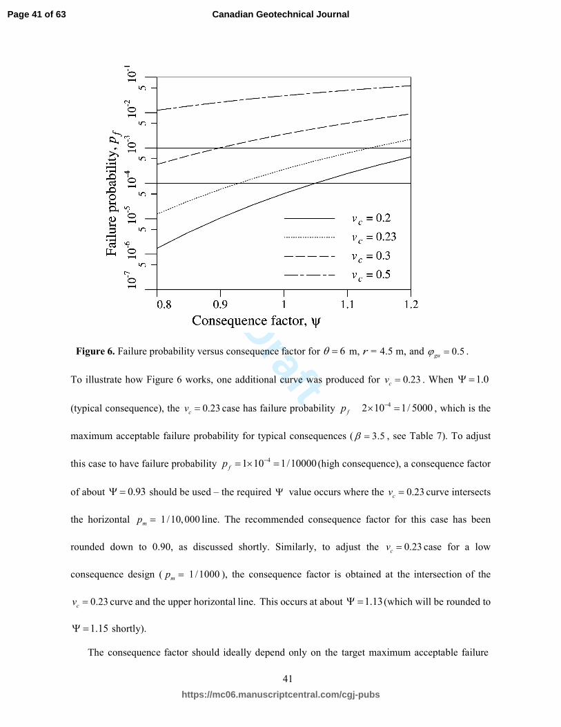
Draft
41
Figure 6. Failure probability versus consequence factor for 6θ = m, r = 4.5 m, and 0.5guϕ = .
To illustrate how Figure 6 works, one additional curve was produced for 0.23cv = . When 1.0Ψ =
(typical consequence), the 0.23cv = case has failure probability 42 10 1/ 5000fp −× =� , which is the
maximum acceptable failure probability for typical consequences ( 3.5β = , see Table 7). To adjust
this case to have failure probability 41 10 1/10000fp −= × = (high consequence), a consequence factor
of about 0.93Ψ = should be used – the required Ψ value occurs where the 0.23cv = curve intersects
the horizontal 1 /10,000mp = line. The recommended consequence factor for this case has been
rounded down to 0.90, as discussed shortly. Similarly, to adjust the 0.23cv = case for a low
consequence design ( 1/1000mp = ), the consequence factor is obtained at the intersection of the
0.23cv = curve and the upper horizontal line. This occurs at about 1.13Ψ = (which will be rounded to
1.15Ψ = shortly).
The consequence factor should ideally depend only on the target maximum acceptable failure
Page 41 of 63
https://mc06.manuscriptcentral.com/cgj-pubs
Canadian Geotechnical Journal
Draft
42
probability, mp , and not on soil variability, correlation length, nor on sampling location. Variations in
the latter three parameters should ideally be entirely handled by the resistance factor, guϕ , which
looks after the issue of site understanding. For the high consequence level case, Fenton et al. (2011)
found that the range in Ψ values (for r ranging from 0 to 9 m, θ ranging from 0 to 50 m, and cv
ranging from 0.1 to 0.5) is from 0.91 to 0.976, a relative change of only about 7%. When compared to
the more than 200% relative change in resistance factors over the same parameter set, it can safely
be concluded that the high consequence factor is largely independent of soil/sampling parameters (θ ,
cv , and r) and primarily dependent on mp . These results were obtained when the resistance factor
was selected as a function of mp , r, θ , and cv to yield 1 / 5000mp = .
For the low consequence level case, Fenton et al. (2011) found the range in Ψ to be from
1.06 to 1.28, a relative change of about 19%. If the 0.5cv = case is ignored, the relative change
drops to about 13%. This is a wider range than achieved for the high consequence level, but still a
small range when compared to the changes in the resistance factor. Again, it appears reasonable to
conclude that the low consequence factor is largely independent of site understanding and primarily
dependent on mp .
When the resistance factor is held fixed with respect to θ and cv , the range in the consequence
factor is increased considerably. For example, when the resistance factor is fixed at 0.4guϕ = for
low understanding (r = 9 m), the consequence factor for the high consequence case varies from
0.38 to 2.47. The equivalent range for the low consequence case is 0.52 to 2.69. More details
can be found in Fenton et al. (2011). Figure 7 shows how the consequence factor varies with the
correlation length, θ , for r = 4.5 m (typical understanding) and 0.5guϕ = .
Considering Figure 7a, the task is to choose a factor for the high consequence case which is
sufficiently conservative and yet not excessively so. Reducing the consequence factor results in
Page 42 of 63
https://mc06.manuscriptcentral.com/cgj-pubs
Canadian Geotechnical Journal
Draft
43
more conservative designs (lower failure probability). A solid horizontal line has been drawn across
the plot at 0.9Ψ = and it can be seen that this value is conservative for all 0.25cv ≤ (approximately)
in that the curves for 0.1cv = and 0.2 lie entirely above 0.9Ψ = . What this means is that if cv is
known to be 0.1, for example, then using 0.9Ψ = in the design would result in a failure probability
well below the target of 1/10,000mp = . On the other hand, if cv is not clearly known, then 0.9Ψ =
is reasonably conservative for all but sites with large soil variability (e.g. 0.3cv ≥ ). If site
investigation is sufficient to keep the residual variability below this level, then 0.9Ψ = is a
reasonable design value for the high failure consequence case which will almost always lead to a
failure probability well below 1/10,000mp = ( 3.7β = ).
A similar argument can be applied to Figure 7b for the low consequence case, where a solid line
at 1.15Ψ = has been drawn across the plot. It can be seen that this value is not quite as conservative
as the high consequence factor (selected above) in that the 0.2cv = curve comes somewhat closer to
1.15Ψ = . The authors feel, however, that conservatism is not quite as important for the low
failure consequence case, and so selected the somewhat less conservative value of 1.15.
Research into the consequence values for deep foundation design (Naghibi et al., 2013) yields
similar consequence factors for both ULS and SLS design. Thus, it appears that the consequence
factors selected for the 2014 CHBDC are reasonably appropriate for any limit state and geotechnical
system.
Page 43 of 63
https://mc06.manuscriptcentral.com/cgj-pubs
Canadian Geotechnical Journal
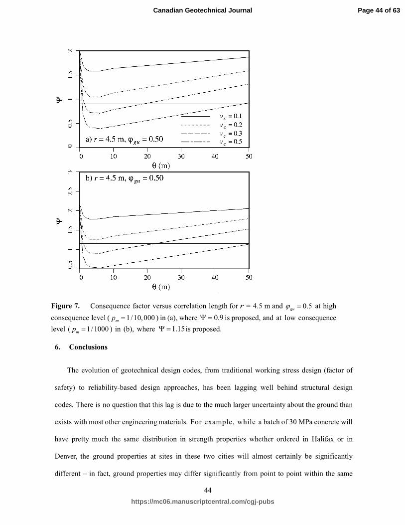
Draft
44
Figure 7. Consequence factor versus correlation length for r = 4.5 m and 0.5guϕ = at high
consequence level ( 1/10,000mp = ) in (a), where 0.9Ψ = is proposed, and at low consequence
level ( 1/1000mp = ) in (b), where 1.15Ψ = is proposed.
6. Conclusions
The evolution of geotechnical design codes, from traditional working stress design (factor of
safety) to reliability-based design approaches, has been lagging well behind structural design
codes. There is no question that this lag is due to the much larger uncertainty about the ground than
exists with most other engineering materials. For example, while a batch of 30 MPa concrete will
have pretty much the same distribution in strength properties whether ordered in Halifax or in
Denver, the ground properties at sites in these two cities will almost certainly be significantly
different – in fact, ground properties may differ significantly from point to point within the same
Page 44 of 63
https://mc06.manuscriptcentral.com/cgj-pubs
Canadian Geotechnical Journal

Draft
45
site.
In general, all sources of uncertainty entering into the LRFD equation (e.g. Eq. 2) are factored to
arrive at an acceptably safe design solution. The factors applied are related to the magnitude of
the uncertainty in the parameter being factored. For example, the uncertainty associated with steel
reinforcing is less than that with concrete and so the steel resistance factor is closer to 1.0 than is
the concrete resistance factor. Reduced uncertainty about an engineering material results in an
increased resistance factor. The ground is simply another engineering material and the resistance
factor associated with the ground should be related to its site specific uncertainty. Since the
distribution of the ground strength varies from site to site and even within a site, it makes sense to
relate the geotechnical resistance factor to the magnitude of the residual uncertainty, i.e. the
uncertainty remaining after site investigation and modeling efforts have been accounted for.
The structural design codes in Canada also recognize the fact that some of the parameters in
the LRFD equation are highly variable and so need to be treated with special consideration in the
event that the system being designed is of higher or lesser importance, i.e. if the failure
consequences are higher or lower than usual. Because earthquake, wind, and snow load are highly
variable and have site specific distributions, both the NBCC and the CHBDC apply importance
factors to these loads. The importance factors increase with increasing system importance.
Similarly, ground properties are both highly variable and site specific, and so the application of a
factor to account for system importance is appropriate on the resistance side, especially in the event
that snow, wind, and seismic loads are not considered for a particular load combination.
With the above thoughts in mind, the 2014 edition of the Canadian Highway Bridge Design
Code includes several philosophical changes to their geotechnical design provisions. The most
important of these are;
• the introduction of three levels of site and model understanding – high, typical, and low –
through the ULS and SLS resistance factors. These factors are intended to account for site
Page 45 of 63
https://mc06.manuscriptcentral.com/cgj-pubs
Canadian Geotechnical Journal
Draft
46
and modeling uncertainties and are aimed at producing a design with a target maximum
acceptable failure probability for typical geotechnical systems (i.e. systems having typical
failure consequence levels). For example, ULS and SLS typical maximum acceptable lifetime
failure probabilities are selected to be 1/5,000 and 1/500, respectively, and so the resistance
factors are targeted at these values.
• the introduction of three levels of failure consequence – high, typical, and low – through a
consequence factor which multiplies the factored resistance. The basic idea of the consequence
factor is to allow the target maximum acceptable lifetime failure probability provided by the
resistance factor to be adjusted up or down depending on whether the failure consequences are
lower or higher than typical.
Research into the determination of the required resistance and consequence factors for the
Canadian codes is ongoing. The consequence factor applied to geotechnical resistance is a new
idea and work is still needed to determine when it should and should not be applied. For example,
the probabilistic effect of applying both the consequence factor to the geotechnical resistance and
importance factors to various load combinations simultaneously is currently unknown.
Acknowledgements
The authors are thankful for the financial support provided by the National Sciences and
Engineering Research Council of Canada and by a Special Research Project Grant from the Ministry
of Transportation of Ontario, Canada, without which the research reported in this paper could not
have been accomplished.
References
Allen, D.E. 1975. “Limit States Design – A probabilistic study,” Can. J. Civ. Engrg., 2(1),36–
49.
Allen, T.M., Nowak, A.S., and Bathurst, R.J. 2005. Calibration to Determine Load and
Page 46 of 63
https://mc06.manuscriptcentral.com/cgj-pubs
Canadian Geotechnical Journal
Draft
47
Resistance Factors for Geotechnical and Structural Design, Transportation Research Circular
Number E-C079, Transportation Research Board, Washington, DC.
American Association of State Highway and Transportation Officials 2012. LRFD Bridge Design
Specifications, Washington, DC.
American Society of Civil Engineers 2010. Minimum Design Loads for Buildings and Other
Structures, ASCE Standard ASCE/SEI 7-10, Reston, Virginia.
Bartlett, F.M., Hong, H.P., and Zhou, W. 2003. “Load factor calibration for the proposed 2005
edition of the National Building Code of Canada: Statistics of loads and load effects,” Can. J.
Civ. Engrg., 30(2), doi: 10.1139/L02-087, 429–439.
Becker, D.E. 1996. “Eighteenth Canadian Geotechnical Colloquium: Limit states design for
foundations. Part 1. An overview of the foundation design process,” Can. Geotech. J., 33(6),
956–983.
Becker, D.E. 1996. “Eighteenth Canadian Geotechnical Colloquium: Limit states design for
foundations. Part II. Development for the National Building Code of Canada,” Can. Geotech. J.,
33(6), 984–1007.
Bond, A. 2013. “Implementation and evolution of Eurocode 7,” in Modern Geotechnical Design
Codes of Practice: Implementation, Application, and Development, Arnold, P., Fenton, G.A.,
Hicks, M.A., Schweckendiek, T., and Simpson, B., eds., Advances in Soil Mechanics and
Geotechnical Engineering, IOS Press, Amsterdam, 3–14.
CEN (European Committee for Standardization) 2002a. EN 1990 Eurocode – Basis of Structural
Design, Brussels.
CEN (European Committee for Standardization) 2002b. EN 1991-1-1 Eurocode 1: Actions on
structures – Part 1-1: General actions – Densities, self-weight, imposed loads for buildings, Brussels.
CEN (European Committee for Standardization) 2003. EN 1991-2 Eurocode 1: Actions on structures –
Part 2: Traffic loads on bridges, Brussels.
CEN (European Committee for Standardization) 2004. EN 1997-1 Eurocode 7: Geotechnical
design – Part 1: General rules, Brussels.
Canadian Geotechnical Society 1992. Canadian Foundation Engineering Manual, 3rd Ed.,
Montreal, Quebec.
Canadian Geotechnical Society 2006. Canadian Foundation Engineering Manual, 4th Ed.,
Montreal, Quebec.
Canadian Standards Association 2014. Canadian Highway Bridge Design Code, CAN/CSA-S6-14,
Mississauga, Ontario.
Page 47 of 63
https://mc06.manuscriptcentral.com/cgj-pubs
Canadian Geotechnical Journal
Draft
48
Canadian Standards Association 2006. Canadian Highway Bridge Design Code, CAN/CSA-S6-06,
Mississauga, Ontario.
Danish Geotechnical Institute 1985. Code of Practice for Foundation Engineering, DGI-Bulletin No.
36, Copenhagen.
D’Appolonia and the University of Michigan 2004. “Load and Resistance Factors for Earth
Pressures on Bridge Substructurs and Retaining Walls” , NCHRP Report 12-55, National
Cooperative Highway Research Program, Transportation Research Board, NRC, Washington,
DC.
Ellingwood, B.R., Galambos, T.V., MacGregor, J.G., and Cornell, C.A. 1980. “Development of a
Probability Based Load Criterion for American National Standard A58: Building Code
Requirements for Minimum Design Loads in Buildings and Other Structures” , National
Bureau of Standards, U.S. Dept. of Commerce, NSC Special Publication 577, Washington,
D.C..
Ellingwood, B.R. 1999. “A Comparison of General Design and Load Requirements in Building
Codes in Canada, Mexico, and the United States,” Engineering Journal, 2, 67–81.
Fenton, G.A. and Griffiths, D.V. 2008. Risk Assessment in Geotechnical Engineering, John Wiley
& Sons, New York.
Fenton, G.A., Griffiths, D.V., and Cavers, W. 2005a. “Resistance factors for settlement design,” Can.
Geotech. J., 42(5), 1422–1436.
Fenton, G.A. Griffiths, D.V., and Williams, M.B. 2005b. “Reliability of traditional retaining wall
design,” Geotechnique, 55(1), 55–62.
Fenton, G.A., Griffiths, D.V., and Zhang, X.Y. 2008. “Load and resistance factor design of
shallow foundations against bearing failure,” Can. Geotech. J., 45(11), 1556-1571.
Fenton, G.A. 2013. “Geotechnical design code development in Canada,” in Modern Geotechnical
Design Codes of Practice: Implementation, Application, and Development, Arnold, P., Fenton,
G.A., Hicks, M.A., Schweckendiek, T., and Simpson, B., eds., Advances in Soil Mechanics
and Geotechnical Engineering, IOS Press, Amsterdam, 277–294.
Fenton, G.A., Griffiths, D.V., and Ojomo, O.O. 2011. “Consequence factors in the ultimate limit state
design of shallow foundations,” Can. Geotech. J., 48(2), 265–279.
Fenton, G.A., and Naghibi, M. 2011. “Geotechnical resistance factors for ultimate limit state
design of deep foundations in frictional soils,” Can. Geotech. J., 48(11), 1742–1756.
French, S.E, 1999. Design of Shallow Foundations, ASCE Press, Reston, Virginia.
Green, R., and Becker, D. 2000. “National report on limit state design in geotechnical engineering:
Page 48 of 63
https://mc06.manuscriptcentral.com/cgj-pubs
Canadian Geotechnical Journal
Draft
49
Canada,” LSD2000: International Workshop on Limit State Design in Geotechnical
Engineering, ISSMGE, TC23, Melbourne, Australia, Nov 18.
Griffiths, D.V., Fenton, G.A., and Tveten, D.E. 2002. “Probabilistic geotechnical analysis: How
difficult does it need to be?,” in Proc. Int. Conf. on Probabilistics in Geotechnics: Technical
and Economic Risk Estimation, Pottler, R., Klapperich, H., and Scheiger, H., eds., United
Engineering Foundation, Graz, Austria, 3–20.
Hicks, M.A. 2013. “An explanation of characteristic values of soil properties in Eurocode7,” in
Modern Geotechnical Design Codes of Practice: Implementation, Application, and
Development, Arnold, P., Fenton, G.A., Hicks, M.A., Schweckendiek, T. and Simpson, B., eds.,
Advances in Soil Mechanics and Geotechnical Engineering, IOS Press, Amsterdam,277–294.
Honjo, Y., Kieu Le, T.C., Hara, T., Shirato, M., Suzuki, M., and Kikuchi, Y. 2009. “Code
calibration in reliability based design level I verification format for geotechnical structures,” in
Geotechnical Risk and Safety, Proceedings of the 2nd International Symposium on Geotech- nical
Safety and Risk (IS-Gifu 2009), Honjo, Y., Hara, T., Suzuki, M., and Zhang, F., eds., CRC
Press, Gifu, Japan, June 11-12, 435–452.
International Organization for Standardization 2015. ISO 2394 General principles on reliability for
structures, Geneva.
Littlejohn, G.S., Arber, N.R., Craig, C., and Forde, M.C. 1991. “Inadequate site investigation,”
Instn. Civ. Engrs., p 1.
Meyerhof, G. G. 1963. “Some recent research on the bearing capacity of foundations,” Can.
Geotech. J., 1(1), 16–26.
Meyerhof, G. G. 1951. “The ultimate bearing capacity of foundations,” Geotechnique, 2(4),301–
332
Meyerhof, G.G. 1995. “Development of geotechnical limit state design,” Can. Geotech. J.,32(1),
128–136.
Naghibi, F., Fenton, G.A., and Griffiths, D.V. 2013. “Resistance and consequence factor
calibration for deep foundations,” Proceedings of the 66th Canadian Geotechnical Conference,
Canadian Geotechnical Society, Sep 29 – Oct 2, Montreal, Paper #224.
Naghibi, F., Fenton, G.A., and Griffiths, D.V. 2014. “Serviceability limit state design of deep
foundations,” Geotechnique, 64(10), 787–799.
Naghibi, M., and Fenton, G.A. 2011. “Geotechnical resistance factors for ultimate limit state
design of deep foundations in cohesive soils,” Can. Geotech. J., 48(11), 1729–1741.
National Research Council 2010. National Building Code of Canada, 13th Ed., National
Page 49 of 63
https://mc06.manuscriptcentral.com/cgj-pubs
Canadian Geotechnical Journal
Draft
50
Research Council of Canada, Ottawa.
National Research Council 2006. User’s Guide – NBC 2005 Structural Commentaries (Part 4 of
Division B), 2nd Ed., National Research Council of Canada, Ottawa.
National Research Council 2011. User’s Guide – NBC 2010 Structural Commentaries (Part 4 of
Division B), 3rd Ed., National Research Council of Canada, Ottawa.
NCHRP 1991. Manuals for the Design of Bridge Foundations, Report 343, National Cooperative
Highway Research Program, Transportation Research Board, NRC, Washington, DC.
Nowak, A.S. 1994. “Calibration of the Ontario Highway Bridge Design Code 1991 edition”, Can. J.
Civ. Eng., 21(1), 25–35.
Nowak, A.S., and Grouni, H.N. 1994. “Load model for bridge design code”, Can. J. Civ. Eng.,
21(1), 36–49.
Phoon, K-K., and Kulhawy, F.H. 1999. “Characterization of geotechnical variability,” Can.
Geotech. J., 36(4), 612–624.
Phoon, K-K., Kulhawy, F.H., and Grigoriu, M.D. 2003. “Multiple resistance factor design
(MRFD) for spread foundations,” J. Geotech. Geoenv. Engrg., American Society of Civil
Engineers, 129(9), 807–818.
Phoon, K-K., and Kulhawy, F.H. 2008. “Serviceability limit state reliability-based design,” in
Reliability-Based Design in Geotechnical Engineering: Computations and Applications, Phoon,
K-K., Ed., CRC Press, Taylor & Francis Group, 344–383.
Prandtl, L. 1921. “Uber die Eindringungsfestigkeit (Harte) plastischer Baustoffe und die Fes-
tigkeit von Schneiden,” Zeitschrift fur angewandte Mathematik und Mechanik, 1(1), 15–20.
Schneider, H.R. 2012. “Dealing with uncertainties in EC7 with emphasis on determination of
characteristic soil properties,” in Modern Geotechnical Design Codes of Practice - Develop-
ment, Calibration & Experiences, Arnold, P., Fenton, G.A., Hicks, M.A., Schweckendiek, T.
and Simpson, B., eds., IOS Press, Amsterdam, The Netherlands.
Smith, I.M., and Griffiths, D.V. 2004. Programming the Finite Element Method, 4th Ed., J. Wiley&
Sons, New York, New York.
Standards Australia 2004a. Bridge Design, Part 1: Scope and General Principles, Australian
Standard AS 5100.1–2004, Sydney, Australia.
Standards Australia 2004b. Bridge Design, Part 3: Foundations and Soil-Supporting Structures,
Australian Standard AS 5100.3–2004, Sydney, Australia.
Standards Australia 2002. Structural Design Actions, Part 1: Permanent, imposed and other
actions, Australian/New Zealand Standard, AS 1170.1:2002, Sydney, Australia.
Page 50 of 63
https://mc06.manuscriptcentral.com/cgj-pubs
Canadian Geotechnical Journal
Draft
51
List of Symbols
The following symbols are used in this paper:
A = footing area
B = footing width
c = cohesion
c = characteristic cohesion
D = effective soil property averaging domain centered under footing =W W×
ˆiF = i
th characteristic load effect
ˆuiF = i
th characteristic load effect at ULS
ˆDF = characteristic dead load, kN/m
ˆLF = characteristic live load, kN/m
sF = Factor of Safety
iI = structure importance factor corresponding to the ith
load effect
Dk = dead load bias factor = ˆ/D DFµ
Lk = extreme lifetime live load bias factor = ˆ/L LFµ
Rk = resistance bias factor = ˆ/R uRµ
ˆcN = characteristic bearing capacity factor
ˆfN = factored characteristic bearing capacity factor
fp = probability of bearing capacity failure
mp = maximum acceptable probability of bearing capacity failure
Q = characteristic soil property averaging domain x H∆ ×
r = distance between soil sample and footing center, m
/D LR = ratio of mean dead load to mean extreme lifetime live load
R = characteristic geotechnical resistance based on characteristic soil properties
ˆuR = characteristic ultimate geotechnical resistance based on characteristic soil properties at ULS
cv = coefficient of variation of cohesion
Dv = coefficient of variation of dead load
Page 51 of 63
https://mc06.manuscriptcentral.com/cgj-pubs
Canadian Geotechnical Journal
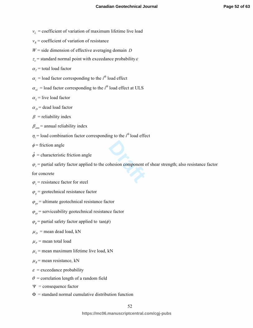
Draft
52
Lv = coefficient of variation of maximum lifetime live load
Rv = coefficient of variation of resistance
W = side dimension of effective averaging domain D
zε = standard normal point with exceedance probabilityε
Tα = total load factor
iα = load factor corresponding to the ith
load effect
uiα = load factor corresponding to the ith
load effect at ULS
Lα = live load factor
Dα = dead load factor
β = reliability index
annβ = annual reliability index
iη = load combination factor corresponding to the ith
load effect
φ = friction angle
φ = characteristic friction angle
cϕ = partial safety factor applied to the cohesion component of shear strength; also resistance factor
for concrete
sϕ = resistance factor for steel
gϕ = geotechnical resistance factor
guϕ = ultimate geotechnical resistance factor
gsϕ = serviceability geotechnical resistance factor
φϕ = partial safety factor applied to tan( )φ
Dµ = mean dead load, kN
Fµ = mean total load
Lµ = mean maximum lifetime live load, kN
Rµ = mean resistance, kN
ε = exceedance probability
θ = correlation length of a random field
Ψ = consequence factor
Φ = standard normal cumulative distribution function
Page 52 of 63
https://mc06.manuscriptcentral.com/cgj-pubs
Canadian Geotechnical Journal
Draft
53
Lω = ratio of zε to reliability index, β
Figure Captions:
Figure 1. Three geotechnical systems having resistance R under load F can have precisely the
same mean factor of safety and yet very different failure probabilities, P[ ]F R> .
Figure 2. Floating partial safety factor, relative to the default, applied to geotechnical resistance
(numbers are for illustration only).
Figure 3. Bearing failure of a shallow foundation on a spatially variable soil.
Figure 4. Locations of footing and sample used in the calibration of bearing capacity resistance
factors.
Figure 5. Resistance factors required to achieve acceptable failure probability, , when soil is sample
under the footing (r = 0 m) in (a), at a distance of r = 4.5 m in (b), and at a distance of r = 9 m in (c).
Figure 6. Failure probability versus consequence factor for 6θ = m, r = 4.5 m, and 0.5guϕ = .
Figure 7. Consequence factor versus correlation length for r = 4.5 m and 0.5guϕ = at high
consequence level ( 1/10,000mp = ) in (a), where 0.9Ψ = is proposed, and at low consequence
level ( 1/1000mp = ) in (b), where 1.15Ψ = is proposed.
Page 53 of 63
https://mc06.manuscriptcentral.com/cgj-pubs
Canadian Geotechnical Journal
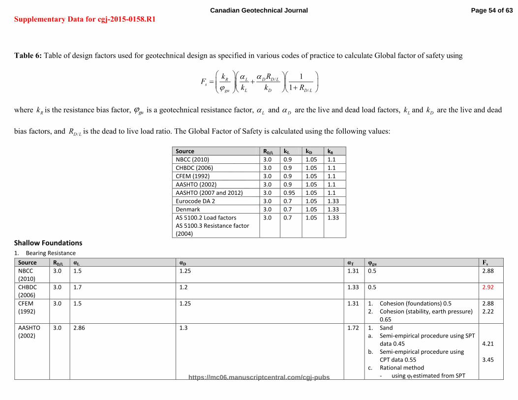
Draft
Supplementary Data for cgj-2015-0158.R1
Table 6: Table of design factors used for geotechnical design as specified in various codes of practice to calculate Global factor of safety using
/
/
1
1
D D LR
L D D L
Ls
gu
Rk
k kF
R
ααϕ
= + +
where Rk is the resistance bias factor, guϕ is a geotechnical resistance factor, Lα and Dα are the live and dead load factors, Lk and Dk are the live and dead
bias factors, and /D LR is the dead to live load ratio. The Global Factor of Safety is calculated using the following values:
Source RD/L kL kD kR
NBCC (2010) 3.0 0.9 1.05 1.1
CHBDC (2006) 3.0 0.9 1.05 1.1
CFEM (1992) 3.0 0.9 1.05 1.1
AASHTO (2002) 3.0 0.9 1.05 1.1
AASHTO (2007 and 2012) 3.0 0.95 1.05 1.1
Eurocode DA 2 3.0 0.7 1.05 1.33
Denmark 3.0 0.7 1.05 1.33
AS 5100.2 Load factors
AS 5100.3 Resistance factor
(2004)
3.0 0.7 1.05 1.33
Shallow Foundations
1. Bearing Resistance
Source RD/L αL αD αT φgu Fs
NBCC
(2010)
3.0 1.5 1.25 1.31 0.5 2.88
CHBDC
(2006)
3.0 1.7 1.2 1.33 0.5 2.92
CFEM
(1992)
3.0 1.5 1.25 1.31 1. Cohesion (foundations) 0.5
2. Cohesion (stability, earth pressure)
0.65
2.88
2.22
AASHTO
(2002)
3.0 2.86 1.3 1.72 1. Sand
a. Semi-empirical procedure using SPT
data 0.45
b. Semi-empirical procedure using
CPT data 0.55
c. Rational method
- using φf estimated from SPT
4.21
3.45
Page 54 of 63
https://mc06.manuscriptcentral.com/cgj-pubs
Canadian Geotechnical Journal

Draft
data 0.35
- using φf estimated from CPT
data 0.45
2. Clay
a. Semi-empirical procedure using
CPT 0.50
b. Rational method
- using shear strength measured
in lab tests0.60
- using shear strength measured
in field vane tests 0.60
c. using shear strength estimated
from CPT data 0.50
3. Rock
Semi-empirical procedure(Carter and
Kulhawy) 0.60
5.42
4.21
3.79
3.16
3.16
3.79
3.16
AASHTO
(2007 and
2012)
3.0 1.75 1.25 1.35 1. Theoretical method(Munfakh et al.,
2001), in clay 0.50
2. Theoretical method(Munfakh et al.,
2001), in sand, using CPT 0.50
3. Theoretical method(Munfakh et al.,
2001), in sand, using SPT 0.45
4. Semi-empirical methods(Meyerhof,
1957), all soils 0.45
5. Footings on rock 0.45
6. Plate Load Test 0.55
2.98
2.98
3.31
3.31
3.31
2.71
Eurocode
DA 2
A1 (load
factors) +
M1
(material
factor =
1.0) + R2
(resistanc
e factor)
3.0 1.5 1.35 1.50 1.0/1.4 = 0.71 2.81
Denmark 3.0 1.3 1.0 1.18 1. Cohesion for bearing capacity of
footings
• Normal 1.0/1.8 = 0.56
• High 1.0/2.0 = 0.5
2. Cohesion for stability and earth
pressures
• Normal 1.0/1.5 = 0.67
• High 1.0/1.65 = 0.61
2.80
3.14
2.34
2.57
Page 55 of 63
https://mc06.manuscriptcentral.com/cgj-pubs
Canadian Geotechnical Journal
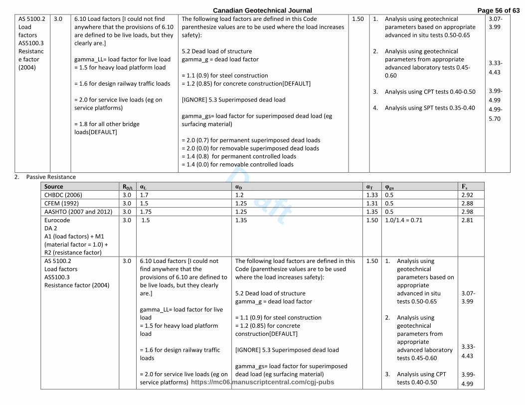
Draft
AS 5100.2
Load
factors
AS5100.3
Resistanc
e factor
(2004)
3.0 6.10 Load factors [I could not find
anywhere that the provisions of 6.10
are defined to be live loads, but they
clearly are.]
gamma_LL= load factor for live load
= 1.5 for heavy load platform load
= 1.6 for design railway traffic loads
= 2.0 for service live loads (eg on
service platforms)
= 1.8 for all other bridge
loads[DEFAULT]
The following load factors are defined in this Code
parenthesize values are to be used where the load increases
safety):
5.2 Dead load of structure
gamma_g = dead load factor
= 1.1 (0.9) for steel construction
= 1.2 (0.85) for concrete construction[DEFAULT]
[IGNORE] 5.3 Superimposed dead load
gamma_gs= load factor for superimposed dead load (eg
surfacing material)
= 2.0 (0.7) for permanent superimposed dead loads
= 2.0 (0.0) for removable superimposed dead loads
= 1.4 (0.8) for permanent controlled loads
= 1.4 (0.0) for removable controlled loads
1.50
1. Analysis using geotechnical
parameters based on appropriate
advanced in situ tests 0.50-0.65
2. Analysis using geotechnical
parameters from appropriate
advanced laboratory tests 0.45-
0.60
3. Analysis using CPT tests 0.40-0.50
4. Analysis using SPT tests 0.35-0.40
3.07-
3.99
3.33-
4.43
3.99-
4.99
4.99-
5.70
2. Passive Resistance
Source RD/L αL αD αT φgu Fs
CHBDC (2006) 3.0 1.7 1.2 1.33 0.5 2.92
CFEM (1992) 3.0 1.5 1.25 1.31 0.5 2.88
AASHTO (2007 and 2012) 3.0 1.75 1.25 1.35 0.5 2.98
Eurocode
DA 2
A1 (load factors) + M1
(material factor = 1.0) +
R2 (resistance factor)
3.0 1.5 1.35 1.50 1.0/1.4 = 0.71 2.81
AS 5100.2
Load factors
AS5100.3
Resistance factor (2004)
3.0 6.10 Load factors [I could not
find anywhere that the
provisions of 6.10 are defined to
be live loads, but they clearly
are.]
gamma_LL= load factor for live
load
= 1.5 for heavy load platform
load
= 1.6 for design railway traffic
loads
= 2.0 for service live loads (eg on
service platforms)
The following load factors are defined in this
Code (parenthesize values are to be used
where the load increases safety):
5.2 Dead load of structure
gamma_g = dead load factor
= 1.1 (0.9) for steel construction
= 1.2 (0.85) for concrete
construction[DEFAULT]
[IGNORE] 5.3 Superimposed dead load
gamma_gs= load factor for superimposed
dead load (eg surfacing material)
1.50
1. Analysis using
geotechnical
parameters based on
appropriate
advanced in situ
tests 0.50-0.65
2. Analysis using
geotechnical
parameters from
appropriate
advanced laboratory
tests 0.45-0.60
3. Analysis using CPT
tests 0.40-0.50
3.07-
3.99
3.33-
4.43
3.99-
4.99
Page 56 of 63
https://mc06.manuscriptcentral.com/cgj-pubs
Canadian Geotechnical Journal

Draft
= 1.8 for all other bridge
loads[DEFAULT]
= 2.0 (0.7) for permanent superimposed dead
loads
= 2.0 (0.0) for removable superimposed dead
loads
= 1.4 (0.8) for permanent controlled loads
= 1.4 (0.0) for removable controlled loads
4. Analysis using SPT
tests 0.35-0.40
4.99-
5.70
3. Horizontal Resistance (Sliding)
Source RD/L αL αD αT φgu Fs
NBCC (2005) 3.0 1.5 1.25 1.31 based on cohesion/adhesion(tan theta = 0) 0.6 2.40
CHBDC (2006) 3.0 1.7 1.2 1.33 0.8 1.83
AASHTO (2002) 3.0 2.85 1.3 1.72 1. Precast concrete placed on sand
a. using φf estimated from SPT data 0.90
b. using φf estimated from CPT data 0.90
2. Concrete cast in place on sand
a. using φf estimated from SPT data 0.80
b. using φf estimated from CPT data 0.80
3. Clay (where shear strength is less than 0.5
times normal pressure)
a. using shear strength measured in lab tests
0.85
b. using shear strength measured in field
tests 0.85
c. using shear strength estimated from CPT
data 0.80
4. Clay (where the strength is greater than
0.5 times normal pressure) 0.85
2.10
2.10
2.37
2.37
2.23
2.23
2.37
2.23
AASHTO (2007
and 2012)
3.0 1.75 1.25 1.35 1. Precast concrete placed on sand 0.90
2. Cast-in-Place Concrete on sand 0.80
3. Cast-in-Place or precast Concrete on Clay
0.85
4. Soil on soil 0.90
5. Passive earth pressure component of
sliding resistance 0.50
1.65
1.86
1.75
1.65
2.98
Eurocode
DA 2
A1 (load factors)
+ M1 (material
factor = 1.0) + R2
(resistance factor)
3.0 1.5 1.35 1.50 1.0/1.1=0.91 2.19
Page 57 of 63
https://mc06.manuscriptcentral.com/cgj-pubs
Canadian Geotechnical Journal

Draft
AS 5100.2
Load factors
AS5100.3
Resistance factor
(2004)
3.0 6.10 Load factors [I
could not find
anywhere that the
provisions of 6.10 are
defined to be live
loads, but they clearly
are.]
gamma_LL= load
factor for live load
= 1.5 for heavy load
platform load
= 1.6 for design
railway traffic loads
= 2.0 for service live
loads (eg on service
platforms)
= 1.8 for all other
bridge loads[DEFAULT]
The following load factors are defined in this Code
(parenthesize values are to be used where the load
increases safety):
5.2 Dead load of structure
gamma_g = dead load factor
= 1.1 (0.9) for steel construction
= 1.2 (0.85) for concrete construction[DEFAULT]
[IGNORE] 5.3 Superimposed dead load
gamma_gs= load factor for superimposed dead load (eg
surfacing material)
= 2.0 (0.7) for permanent superimposed dead loads
= 2.0 (0.0) for removable superimposed dead loads
= 1.4 (0.8) for permanent controlled loads
= 1.4 (0.0) for removable controlled loads
1.50
1. Analysis using geotechnical
parameters based on appropriate
advanced in situ tests 0.50-0.65
2. Analysis using geotechnical parameters
from appropriate advanced laboratory
tests 0.45-0.60
3. Analysis using CPT tests 0.40-0.50
4. Analysis using SPT tests 0.35-0.40
3.07-
3.99
3.33-
4.43
3.99-
4.99
4.99-
5.70
Deep Foundations (Axially Loaded Piles and Drilled Shafts)
1. Resistance to axial load
Source RD/L αL αD αT φgu Fs
NBCC
(2005)
3.0 1.5 1.25 1.31 1. semi-empirical analysis using laboratory
and in-situ test data 0.4
2. analysis using static loading test results
0.6
3. analysis using dynamic monitoring results
0.5
3.60
2.40
2.88
CHBDC
(2006)
3.0 1.7 1.2 1.33 1. Static Analysis
a. Compression 0.4
b. Tension 0.3
2. Static Test
a. Compression 0.6
b. Tension 0.4
3. Dynamic Analysis Compression 0.4
4. Dynamic Test Compression (field
measurement and analysis) 0.5
3.60
4.80
2.40
3.60
3.60
2.88
AASHTO
(2002)
3.0 2.85 1.3 1.72 Piles
1. Skin Friction
a. Alpha-method 0.7
b. Beta-method 0.5
2.70
3.78
Page 58 of 63
https://mc06.manuscriptcentral.com/cgj-pubs
Canadian Geotechnical Journal

Draft
c. Lambda-method 0.55
2. End bearing
a. Clay (Skempton, 1951) 0.70
b. Sand (Kulhawy, 1983)
i. Phi-f from CPT 0.45
ii. Phi-f from SPT 0.35
c. Rock (Canadian Geotech. Society
1985) 0.5
3. Skin Friction and end bearing
a. SPT-method 0.45
b. CPT-method 0.55
c. Load test 0.80
d. Pile driving analyzer 0.70
Single drilled shafts
1. Side resistance in clay
a. Alpha-method (Reese & O’Neill) 0.65
2. Base resistance in clay
a. Total Stress (Reese & O’Neill) 0.55
3. Side resistance in sand
a. Touma & Reese
b. Meyerhof
c. Quiros & Reese
d. Reese & Wright
e. Reese & O’Neill
4. Base resistance in sand
a. Touma & Reese
b. Meyerhof
c. Quiros & Reese
d. Reese & Wright
e. Reese & O’Neill
5. Side resistance in rock
a. Carter & Kulhawy 0.55
b. Horvah and Kenney 0.65
6. Base resistance in rock
a. Canadian Geotechnical Society 0.50
b. Pressuremeter Method(Canadian
Geotechnical Society) 0.50
7. Side resistance and end bearing
a. Load test 0.80
3.44
2.70
4.21
5.41
3.78
4.21
3.44
2.37
2.70
2.91
3.44
3.44
2.91
3.78
3.78
2.37
AASHTO
(2007 and
2012)
3.0 1.75 1.25 1.35 1. Nominal Resistance of Single Pile in Axial
Compression – Dynamic Analysis and
Static Load Test Method
a. Driving criteria established by static
load test(s); quality control by
dynamic testing and/or calibrated
Page 59 of 63
https://mc06.manuscriptcentral.com/cgj-pubs
Canadian Geotechnical Journal

Draft
wave equation, or minimum driving
resistance combined with minimum
delivered hammer energy from the
load test(s). For the last case, the
hammer used for the test pile(s)
shall be used for the production
piles. (See Table 10.5.5.2.3-2) 0.55-
0.90
b. Driving criteria established by
dynamic test with signal matching at
beginning of redrive conditions only
of at least one production pile per
pier, but no less than the number of
tests per site provided in Table 3
Quality control of remaining piles by
calibrated wave equation and/or
dynamic testing 0.65
c. Wave equation analysis, without pile
dynamic measurements or load test,
at end of drive conditions only 0.40
d. FHWA-modified Gates dynamic pile
formula (End of Drive condition only)
0.40
e. Engineering News Record dynamic
pile formula(End of Drive condition
only) 0.10
2. Nominal Resistance of Single Pile in Axial
Compression – Static Analysis Methods
a. Skin Friction and End Bearing: Clay
and Mixed Soils
i. Alpha-method (Tomlinson,
1987; Skempton, 1951) 0.35
ii. Beta-method (Esrig & Kriby,
1979; Skempton, 1951) 0.25
iii. Lambda-method (Vijayvergiya &
Focht, 1972; Skempton, 1951)
0.40
b. Skin Friction and End Bearing: Sand
i. Nordlund/Thurman Method
(Hanningan et al., 2005) 0.45
ii. SPT-method (Myerhof) 0.30
iii. CPT-method (Schmertmann) 0.5
iv. End bearing in rock (Canadian
Geotech Society 1985) 0.45
3. Nominal Axial Compressive Resistance of
1.65-
2.71
2.29
3.72
3.72
14.89
4.25
5.95
3.72
3.31
4.96
2.98
3.31
Page 60 of 63
https://mc06.manuscriptcentral.com/cgj-pubs
Canadian Geotechnical Journal
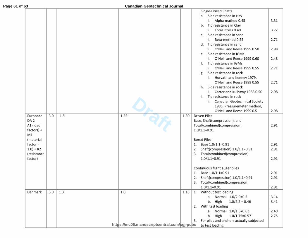
Draft
Single-Drilled Shafts
a. Side resistance in clay
i. Alpha-mathod 0.45
b. Tip resistance in Clay
i. Total Stress 0.40
c. Side resistance in sand
i. Beta-method 0.55
d. Tip resistance in sand
i. O’Neill and Reese 1999 0.50
e. Side resistance in IGMs
i. O’Neill and Reese 1999 0.60
f. Tip resistance in IGMs
i. O’Neill and Reese 1999 0.55
g. Side resistance in rock
i. Horvath and Kenney 1979,
O’Neill and Reese 1999 0.55
h. Side resistance in rock
i. Carter and Kulhawy 1988 0.50
i. Tip resistance in rock
i. Canadian Geotechnical Society
1985, Pressuremeter method,
O’Neill and Reese 1999 0.5
3.31
3.72
2.71
2.98
2.48
2.71
2.71
2.98
2.98
Eurocode
DA 2
A1 (load
factors) +
M1
(material
factor =
1.0) + R2
(resistance
factor)
3.0 1.5 1.35
1.50 Driven Piles
Base, Shaft(compression), and
Total/combined(compression)
1.0/1.1=0.91
Bored Piles
1. Base 1.0/1.1=0.91
2. Shaft(compression) 1.0/1.1=0.91
3. Total/combined(compression)
1.0/1.1=0.91
Continuous flight auger piles
1. Base 1.0/1.1=0.91
2. Shaft(compression) 1.0/1.1=0.91
3. Total/combined(compression)
1.0/1.1=0.91
2.91
2.91
2.91
2.91
2.91
2.91
2.91
Denmark 3.0 1.3 1.0 1.18 1. Without test loading
a. Normal 1.0/2.0=0.5
b. High 1.0/2.2 = 0.46
2. With test loading
a. Normal 1.0/1.6=0.63
b. High 1.0/1.75=0.57
3. For piles and anchors actually subjected
to test loading
3.14
3.41
2.49
2.75
Page 61 of 63
https://mc06.manuscriptcentral.com/cgj-pubs
Canadian Geotechnical Journal

Draft
a. Normal 1.0/1.4=0.71
b. High 1.0/1.55=0.65
2.21
2.41
AS 5100.2
Load
factors
AS5100.3
Resistance
factor
(2004)
3.0 6.10 Load factors [I could not find
anywhere that the provisions of
6.10 are defined to be live loads,
but they clearly are.]
gamma_LL= load factor for live load
= 1.5 for heavy load platform load
= 1.6 for design railway traffic loads
= 2.0 for service live loads (eg on
service platforms)
= 1.8 for all other bridge
loads[DEFAULT]
The following load factors are
defined in this Code (parenthesize
values are to be used where the
load increases safety):
5.2 Dead load of structure
gamma_g = dead load factor
= 1.1 (0.9) for steel construction
= 1.2 (0.85) for concrete
construction[DEFAULT]
[IGNORE] 5.3 Superimposed dead
load
gamma_gs= load factor for
superimposed dead load (eg
surfacing material)
= 2.0 (0.7) for permanent
superimposed dead loads
= 2.0 (0.0) for removable
superimposed dead loads
= 1.4 (0.8) for permanent
controlled loads
= 1.4 (0.0) for removable controlled
loads
1.50
1. static load testing to failure 0.70-0.90
2. static proof load testing 0.70-0.90
3. dynamic load testing supported by signal
matching 0.65-0.85
4. dynamic load testing not supported by
signal matching 0.50-0.70
5. static analysis using CPT data 0.45-0.65
6. static analysis using SPT data in
cohesionless soils 0.40-0.55
7. static analysis using laboratory data in
cohesionless soils 0.45-0.55
8. dynamic analysis using wave equation
method 0.45-0.55
9. dynamic analysis using driving equation
for piles in rock 0.50-0.65
10. dynamic analysis using driving equation
for piles in sand 0.45-0.55
11. measurement during installation of
proprietary displacement piles, using
well-established in-house equation. 0.50-
0.65
2.22-
2.85
2.22-
2.85
2.35-
3.07
2.85-
3.99
3.07-
4.43
3.63-
4.99
3.63-
4.43
3.63-
4.43
3.07-
3.99
3.63-
4.43
3.07-
3.99
2. Horizontal load resistance
Source RD/L αL αD αT φgu Fs
NBCC (2005) 3.0 1.5 1.25 1.31 0.5 2.88
CHBDC (2006) 3.0 1.7 1.2 1.33 0.5 2.92
AASHTO (2007 and 2012) 3.0 1.75 1.25 1.35 Piles - All soils and rock 1.0
Shafts - All materials 1.0
1.49
1.49
3. Block Failure (Group Resistance to axial load)
Source RD/L αL αD αT φgu Fs
AASHTO (2002) 3.0 2.85 1.3 1.72 Piles – Clay 0.65
Shafts - Clay 0.65
2.91
2.91
AASHTO (2007 and 2012) 3.0 1.75 1.25 1.35 Piles - Clay 0.60
Shafts - Clay 0.55
2.48
2.71
4. Uplift capacity
Page 62 of 63
https://mc06.manuscriptcentral.com/cgj-pubs
Canadian Geotechnical Journal
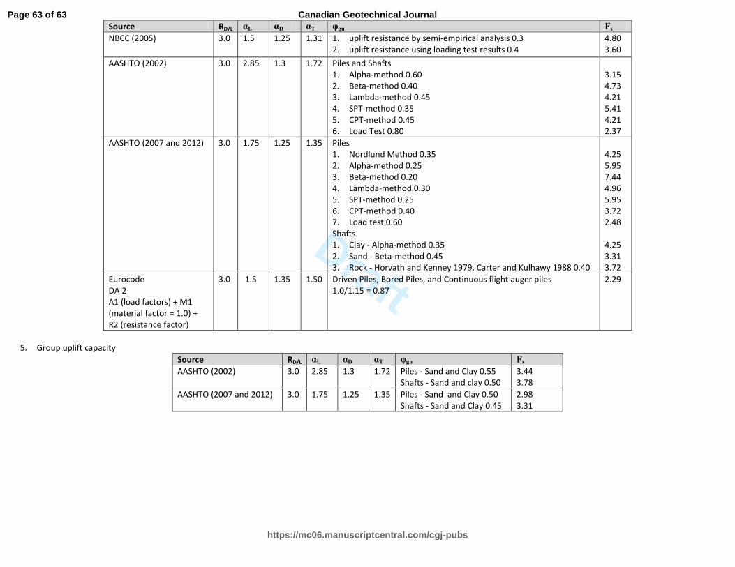
Draft
Source RD/L αL αD αT φgu Fs
NBCC (2005) 3.0 1.5 1.25
1.31 1. uplift resistance by semi-empirical analysis 0.3
2. uplift resistance using loading test results 0.4
4.80
3.60
AASHTO (2002) 3.0 2.85 1.3 1.72 Piles and Shafts
1. Alpha-method 0.60
2. Beta-method 0.40
3. Lambda-method 0.45
4. SPT-method 0.35
5. CPT-method 0.45
6. Load Test 0.80
3.15
4.73
4.21
5.41
4.21
2.37
AASHTO (2007 and 2012) 3.0 1.75 1.25 1.35 Piles
1. Nordlund Method 0.35
2. Alpha-method 0.25
3. Beta-method 0.20
4. Lambda-method 0.30
5. SPT-method 0.25
6. CPT-method 0.40
7. Load test 0.60
Shafts
1. Clay - Alpha-method 0.35
2. Sand - Beta-method 0.45
3. Rock - Horvath and Kenney 1979, Carter and Kulhawy 1988 0.40
4.25
5.95
7.44
4.96
5.95
3.72
2.48
4.25
3.31
3.72
Eurocode
DA 2
A1 (load factors) + M1
(material factor = 1.0) +
R2 (resistance factor)
3.0 1.5 1.35
1.50 Driven Piles, Bored Piles, and Continuous flight auger piles
1.0/1.15 = 0.87
2.29
5. Group uplift capacity
Source RD/L αL αD αT φgu Fs
AASHTO (2002) 3.0 2.85 1.3 1.72 Piles - Sand and Clay 0.55
Shafts - Sand and clay 0.50
3.44
3.78
AASHTO (2007 and 2012) 3.0 1.75 1.25 1.35 Piles - Sand and Clay 0.50
Shafts - Sand and Clay 0.45
2.98
3.31
Page 63 of 63
https://mc06.manuscriptcentral.com/cgj-pubs
Canadian Geotechnical Journal